Embed Size (px)
Citation preview
Statistical Design and Analysis of Experiments
Part Two
Lecture notes
Fall semester 2007
Henrik Spliid
Informatics and Mathematical Modelling
Technical University of Denmark
1
0.1
List of contents, cont.
6.1: Factorial experiments - introduction
6.7: Blocking in factorials
6.9: montgomery example p. 164
6.11: Interaction plot
6.14: Normal probability plot for residuals
7.1: Factorial experiments with two level factors
7.7: A (very) small example of a 2×2 design
2
0.2
7.10: Yates algorithm by an example
7.12: Numerical example with 3 factors
8.1: Block designs for two level factorials
8.5: How-to-do blocking by confounding
8.6: Yates algorithm and blocking
8.7: The confounded block design (what happens?)
8.9: Construction of block design by the tabular method
8.12: A few generalizations on block designs
8.14: The tabular method for 2× blocks (example)
8.15: Partially confounded two level experiments
3
0.3
8.20: Generalization of partial confounding calculations
8.21: Example of partially confounded design
9.1: Fractional designs for two level factorials
9.3: Alternative method of construction (tabular method)
9.7: Generator equation and alias relations
9.8: Analysis of data and the underlying factorial
9.12: 5 factors in 8 measuremets
9.13: Alias relations for model without high order interactions
9.14: Construction of 1/4times25 design (tabular method)
4
0.4
10.1: A large example on 2 level factorials
10.11: Summary of analyses (example)
10.12: Combining main effects and interaction estimates
5
6.1
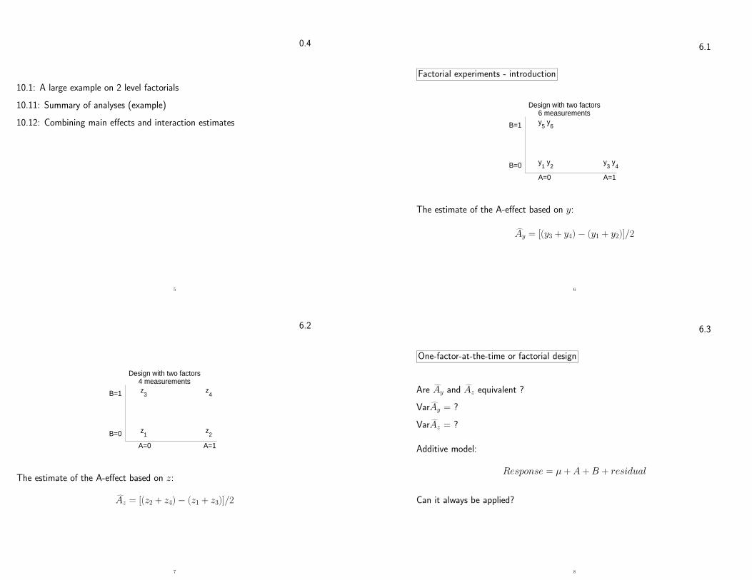
Factorial experiments - introduction
Design with two factors6 measurements
y1 y
2y
3 y
4
y5 y
6B=1
B=0
A=0 A=1
The estimate of the A-effect based on y:
Ay = [(y3 + y4) − (y1 + y2)]/2
6
6.2
Design with two factors4 measurements
z1 z
2
z3 z
4 B=1
B=0
A=0 A=1
The estimate of the A-effect based on z:
Az = [(z2 + z4) − (z1 + z3)]/2
7
6.3
One-factor-at-the-time or factorial design
Are Ay and Az equivalent ?
Var Ay = ?
Var Az = ?
Additive model:
Response = µ + A + B + residual
Can it always be applied?
8
6.4
More complicated model:
Response = µ + A + B + AB + residual
Is it more needed for factorial designs than for block designs, for example, whereadditivity is often assumed?
If interaction is present, then: which design is best ?
Usage of measurements: which design is best ?
In general: How should a factorial experiment be carried out ?
9
6.5
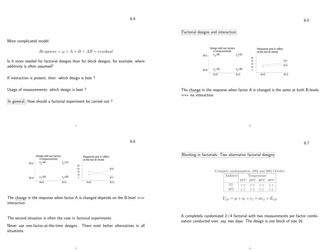
Factorial designs and interaction
Design with two factors4 measurements
z1=20 z
2=40
z3=30 z
4=52 B=1
B=0
A=0 A=1
Response and A−effectat the two B−levels
B=0
B=1
0
20
40
60
80
A=0 A=1
The change in the response when factor A is changed is the same at both B-levels⇐⇒ no interaction
10
6.6
Design with two factors4 measurements
z1=20 z
2=50
z3=40 z
4=12 B=1
B=0
A=0 A=1
Response and A−effectat the two B−levels
B=0
B=1 0
20
40
60
80
A=0 A=1
The change in the response when factor A is changed depends on the B-level ⇐⇒interaction
The second situation is often the case in factorial experiments
Never use one-factor-at-the-time designs. There exist better alternatives in allsituations.
11
6.7
Blocking in factorials: Two alternative factorial designs
Complete randomization, 19th and 20th October
Additive Temperature
10oC 20oC 30oC 40oC
5% y y y y y y y y
10% y y y y y y y y
Yijk = µ + ai + cj + acij + Eijk
A completely randomized 2×4 factorial with two measurements per factor combi-nation conducted over, say, two days. The design is one block of size 16.
12
6.8
Replication 1, October 19th
Additive Temperature
10oC 20oC 30oC 40oC
5% y y y y
10% y y y y
Replication 2, October 20th
Additive Temperature
10oC 20oC 30oC 40oC
5% y y y y
10% y y y y
Yijk = µ + ai + cj + acij + Dayk + Zijk
A completely randomized 2×4 factorial with one measurement per factor combi-nation, but replicated twice, one replication per day, i.e. two blocks of size 8.
Never use the first design. Why ?
13
6.9
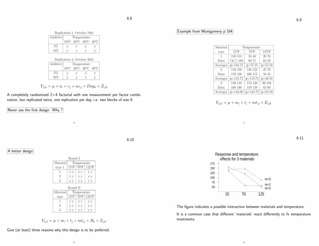
Example from Montgomery p 164
Material Temperature
type 15oF 70oF 125oF
1 130 155 34 40 20 70
Data 74(?) 180 80 75 82 58
Averages y=134.75 y=57.25 y=57.50
2 150 188 136 122 25 70
Data 159 126 106 115 58 45
Averages y=155.75 y=119.75 y=49.50
3 138 110 174 120 96 104
Data 168 160 150 139 82 60
Averages y=144.00 y=145.75 y=85.50
Yijk = µ + mi + tj + mtij + Eijk
14
6.10
A better design
Round I
Material Temperature
type 1 15oF 70oF 125oF
1 y y y y y y
2 y y y y y y
3 y y y y y y
Round II
Material Temperature
type 15oF 70oF 125oF
1 y y y y y y
2 y y y y y y
3 y y y y y y
Yijk = µ + mi + tj + mtij + Rk + Zijk
Give (at least) three reasons why this design is to be preferred.
15
6.11
Response and temperatureeffects for 3 materials
m=1m=2
m=3
50
75
100
125
150
175
15 70 125
The figure indicates a possible interaction between materials and temperature.
It is a common case that different ’materials’ react differently to fx temperaturetreatments.
16
6.12
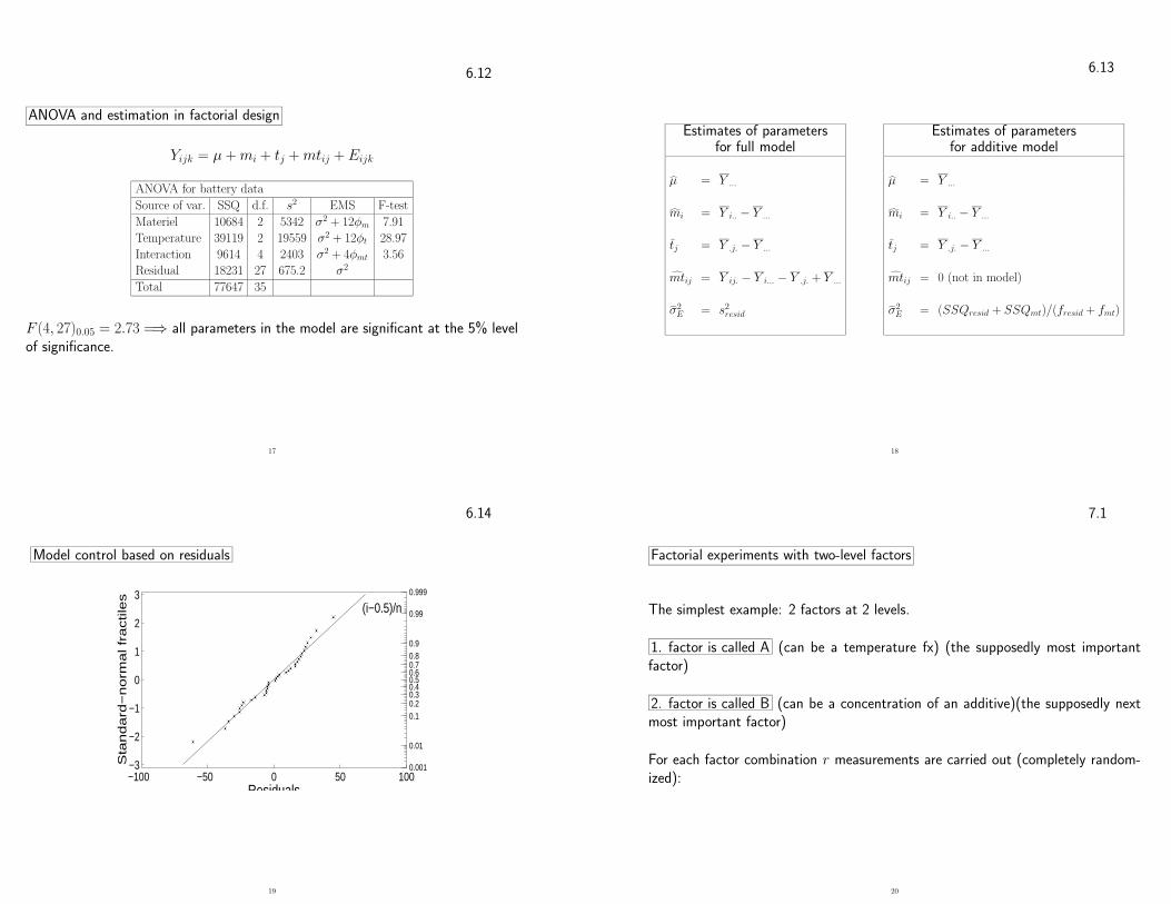
ANOVA and estimation in factorial design
Yijk = µ + mi + tj + mtij + Eijk
ANOVA for battery data
Source of var. SSQ d.f. s2 EMS F-test
Materiel 10684 2 5342 σ2 + 12φm 7.91
Temperature 39119 2 19559 σ2 + 12φt 28.97
Interaction 9614 4 2403 σ2 + 4φmt 3.56
Residual 18231 27 675.2 σ2
Total 77647 35
F (4, 27)0.05 = 2.73 =⇒ all parameters in the model are significant at the 5% levelof significance.
17
6.13
Estimates of parametersfor full model
µ = Y ...
mi = Y i.. − Y ...
tj = Y .j. − Y ...
mtij = Y ij. − Y i... − Y .j. + Y ...
σ2E = s2
resid
Estimates of parametersfor additive model
µ = Y ...
mi = Y i.. − Y ...
tj = Y .j. − Y ...
mtij = 0 (not in model)
σ2E = (SSQresid + SSQmt)/(fresid + fmt)
18
6.14
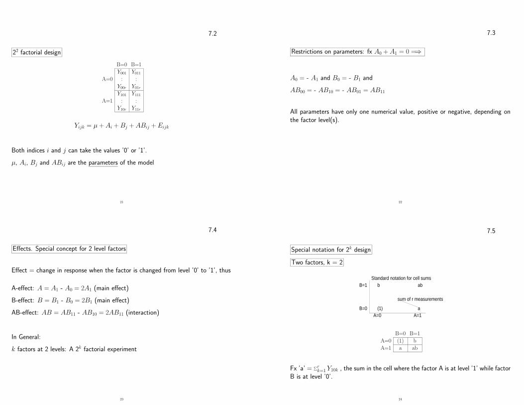
Model control based on residuals
−100 −50 0 50 100−3
−2
−1
0
1
2
3
Sta
nd
ard
−n
orm
al fr
actile
s
Residuals
0.001
0.01
0.10.20.30.40.50.60.70.80.9
0.99
0.999
(i−0.5)/n
19
7.1
Factorial experiments with two-level factors
The simplest example: 2 factors at 2 levels.
1. factor is called A (can be a temperature fx) (the supposedly most importantfactor)
2. factor is called B (can be a concentration of an additive)(the supposedly nextmost important factor)
For each factor combination r measurements are carried out (completely random-ized):
20
7.2
22 factorial design
B=0 B=1
Y001 Y011
A=0 : :
Y00r Y01r
Y101 Y111
A=1 : :
Y10r Y11r
Yijk = µ + Ai + Bj + ABij + Eijk
Both indices i and j can take the values ’0’ or ’1’.
µ, Ai, Bj and ABij are the parameters of the model
21
7.3
Restrictions on parameters: fx A0 + A1 = 0 =⇒
A0 = - A1 and B0 = - B1 and
AB00 = - AB10 = - AB01 = AB11
All parameters have only one numerical value, positive or negative, depending onthe factor level(s).
22
7.4
Effects. Special concept for 2 level factors
Effect = change in response when the factor is changed from level ’0’ to ’1’, thus
A-effect: A = A1 - A0 = 2A1 (main effect)
B-effect: B = B1 - B0 = 2B1 (main effect)
AB-effect: AB = AB11 - AB10 = 2AB11 (interaction)
In General:
k factors at 2 levels: A 2k factorial experiment
23
7.5
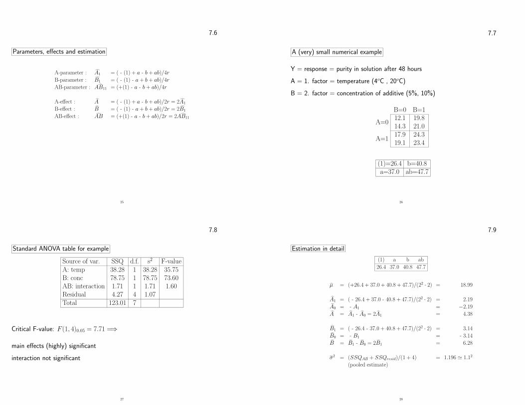
Special notation for 2k design
Two factors, k = 2
Standard notation for cell sums
(1) a
sum of r measurements
b abB=1
B=0A=0 A=1
B=0 B=1
A=0 (1) b
A=1 a ab
Fx ’a’ = ∑rk=1 Y10k , the sum in the cell where the factor A is at level ’1’ while factor
B is at level ’0’.
24
7.6
Parameters, effects and estimation
A-parameter : A1 = ( - (1) + a - b + ab)/4r
B-parameter : B1 = ( - (1) - a + b + ab)/4r
AB-parameter : AB11 = (+(1) - a - b + ab)/4r
A-effect : A = ( - (1) + a - b + ab)/2r = 2A1
B-effect : B = ( - (1) - a + b + ab)/2r = 2B1
AB-effect : AB = (+(1) - a - b + ab)/2r = 2 AB11
25
7.7
A (very) small numerical example
Y = response = purity in solution after 48 hours
A = 1. factor = temperature (4oC , 20oC)
B = 2. factor = concentration of additive (5%, 10%)
B=0 B=1
A=012.114.3
19.821.0
A=117.919.1
24.323.4
(1)=26.4 b=40.8a=37.0 ab=47.7
26
7.8
Standard ANOVA table for example
Source of var. SSQ d.f. s2 F-valueA: temp 38.28 1 38.28 35.75B: conc 78.75 1 78.75 73.60AB: interaction 1.71 1 1.71 1.60Residual 4.27 4 1.07Total 123.01 7
Critical F-value: F (1, 4)0.05 = 7.71 =⇒
main effects (highly) significant
interaction not significant
27
7.9
Estimation in detail
(1) a b ab
26.4 37.0 40.8 47.7
µ = (+26.4 + 37.0 + 40.8 + 47.7)/(22 · 2) = 18.99
A1 = ( - 26.4 + 37.0 - 40.8 + 47.7)/(22 · 2) = 2.19
A0 = - A1 = −2.19
A = A1 - A0 = 2A1 = 4.38
B1 = ( - 26.4 - 37.0 + 40.8 + 47.7)/(22 · 2) = 3.14
B0 = - B1 = - 3.14
B = B1 - B0 = 2B1 = 6.28
σ2 = (SSQAB + SSQresid)/(1 + 4) = 1.196 ' 1.12
(pooled estimate)
28
7.10
Yates algorithm, testing and estimation
Yates algorithm for k = 2 factorsCell sums I II = contrasts SSQ Effects(1) = 26.4 63.4 151.9 = [I] − µ = 18.99a = 37.0 88.5 17.5 = [A] 38.25 A = 4.38b = 40.8 10.6 25.1 = [B] 78.75 B = 6.28ab = 47.7 6.9 - 3.7 = [AB] 1.71 AB = - 0.93
The important concept about Yates’ algorithm is that isrepresents the transformation of the data to the contrasts -and subsequently to the estimates and the sums of squares!
29
7.11
Explanation:
Cell sums: Organized in ’standard order’: (1), a, b, ab
Column I:63.4 = +26.4+37.0 (sum of two first in previous column)
88.5 = +40.8+47.7 (sum of two next)
10.6 = - 26.4+37.0 (reverse difference of two first)
6.9 = - 40.8+47.7 (reverse difference of two next)
Column II: Same procedure as for column I (63.4+88.5=151.9)
SSQA: [A]2/(2k · 2) = 38.25 (k=2) and likewise for B and AB
A-Effect: A = [A]/(2k−1 · 2) = 4.38 and likewise for B and AB
The procedure for column I is repeated k times for the 2k design
The sums of squares and effects appear in the ’standard order’
30
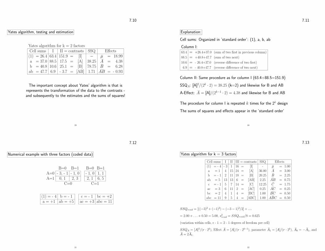
7.12
Numerical example with three factors (coded data)
B=0 B=1A=0 - 3, - 1 - 1, 0A=1 0, 1 2, 3
C=0
B=0 B=1- 1, 0 1, 12, 1 6, 5
C=1
(1) = - 4 b = - 1a = +1 ab = +5
c = - 1 bc = +2ac = +3 abc = 11
31
7.13
Yates algorithm for k = 3 factors
Cell sums I II III = contrasts SSQ Effects
(1) = - 4 - 3 1 16 = [I] - µ = 1.00
a = 1 4 15 24 = [A] 36.00 A = 3.00
b = - 1 2 11 18 = [B] 20.25 B = 2.25
ab = 5 13 13 6 = [AB] 2.25 AB = 0.75
c = - 1 5 7 14 = [C] 12.25 C = 1.75
ac = 3 6 11 2 = [AC] 0.25 AC = 0.25
bc = 2 4 1 4 = [BC] 1.00 BC = 0.50
abc = 11 9 5 4 = [ABC] 1.00 ABC = 0.50
SSQresid = [((−3)2 + (−1)2) − (−3 − 1)2/2] + ....
= 2.00 + . . . + 0.50 = 5.00, s2resid = SSQresid/8 = 0.625
(variation within cells, r - 1 = 2 - 1 degrees of freedom per cell)
SSQA = [A]2/(r · 2k), Effect A = [A]/(r · 2k−1), parameter A1 = [A]/(r · 2k), A0 = −A1, and
A = 2A1.
32
8.1
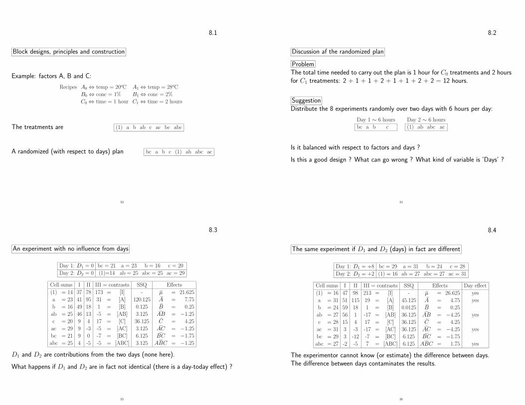
Block designs, principles and construction
Example: factors A, B and C:
Recipes A0 ⇔ temp = 20oC A1 ⇔ temp = 28oC
B0 ⇔ conc = 1% B1 ⇔ conc = 2%
C0 ⇔ time = 1 hour C1 ⇔ time = 2 hours
The treatments are (1) a b ab c ac bc abc
A randomized (with respect to days) plan bc a b c (1) ab abc ac
33
8.2
Discussion af the randomized plan
ProblemThe total time needed to carry out the plan is 1 hour for C0 treatments and 2 hoursfor C1 treatments: 2 + 1 + 1 + 2 + 1 + 1 + 2 + 2 = 12 hours.
SuggestionDistribute the 8 experiments randomly over two days with 6 hours per day:
Day 1 ∼ 6 hours Day 2 ∼ 6 hours
bc a b c (1) ab abc ac
Is it balanced with respect to factors and days ?
Is this a good design ? What can go wrong ? What kind of variable is ’Days’ ?
34
8.3
An experiment with no influence from days
Day 1: D1 = 0 bc = 21 a = 23 b = 16 c = 20
Day 2: D2 = 0 (1)=14 ab = 25 abc = 25 ac = 29
Cell sums I II III = contrasts SSQ Effects
(1) = 14 37 78 173 = [I] - µ = 21.625
a = 23 41 95 31 = [A] 120.125 A = 7.75
b = 16 49 18 1 = [B] 0.125 B = 0.25
ab = 25 46 13 -5 = [AB] 3.125 AB = −1.25
c = 20 9 4 17 = [C] 36.125 C = 4.25
ac = 29 9 -3 -5 = [AC] 3.125 AC = −1.25
bc = 21 9 0 -7 = [BC] 6.125 BC = −1.75
abc = 25 4 -5 -5 = [ABC] 3.125 ABC = −1.25
D1 and D2 are contributions from the two days (none here).
What happens if D1 and D2 are in fact not identical (there is a day-today effect) ?
35
8.4
The same experiment if D1 and D2 (days) in fact are different
Day 1: D1 = +8 bc = 29 a = 31 b = 24 c = 28
Day 2: D2 = +2 (1) = 16 ab = 27 abc = 27 ac = 31
Cell sums I II III = contrasts SSQ Effects Day effect
(1) = 16 47 98 213 = [I] - µ = 26.625 yes
a = 31 51 115 19 = [A] 45.125 A = 4.75 yes
b = 24 59 18 1 = [B] 0.0125 B = 0.25
ab = 27 56 1 -17 = [AB] 36.125 AB = −4.25 yes
c = 28 15 4 17 = [C] 36.125 C = 4.25
ac = 31 3 -3 -17 = [AC] 36.125 AC = −4.25 yes
bc = 29 3 -12 -7 = [BC] 6.125 BC = −1.75
abc = 27 -2 -5 7 = [ABC] 6.125 ABC = 1.75 yes
The experimentor cannot know (or estimate) the difference between days.The difference between days contaminates the results.
36
8.5
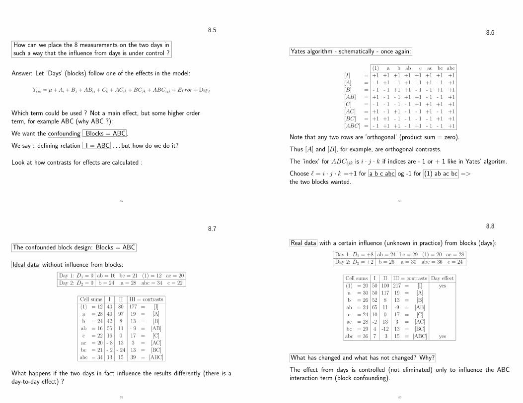
How can we place the 8 measurements on the two days insuch a way that the influence from days is under control ?
Answer: Let ’Days’ (blocks) follow one of the effects in the model:
Yijk = µ + Ai + Bj + ABij + Ck + ACik + BCjk + ABCijk + Error + Day`
Which term could be used ? Not a main effect, but some higher orderterm, for example ABC (why ABC ?):
We want the confounding Blocks = ABC .
We say : defining relation I = ABC . . . but how do we do it?
Look at how contrasts for effects are calculated :
37
8.6
Yates algorithm - schematically - once again:
(1) a b ab c ac bc abc
[I ] = +1 +1 +1 +1 +1 +1 +1 +1
[A] = - 1 +1 - 1 +1 - 1 +1 - 1 +1
[B] = - 1 - 1 +1 +1 - 1 - 1 +1 +1
[AB] = +1 - 1 - 1 +1 +1 - 1 - 1 +1
[C] = - 1 - 1 - 1 - 1 +1 +1 +1 +1
[AC] = +1 - 1 +1 - 1 - 1 +1 - 1 +1
[BC] = +1 +1 - 1 - 1 - 1 - 1 +1 +1
[ABC] = - 1 +1 +1 - 1 +1 - 1 - 1 +1
Note that any two rows are ’orthogonal’ (product sum = zero).
Thus [A] and [B], for example, are orthogonal contrasts.
The ’index’ for ABCijk is i · j · k if indices are - 1 or + 1 like in Yates’ algoritm.
Choose ` = i · j · k =+1 for a b c abc og -1 for (1) ab ac bc =>the two blocks wanted.
38
8.7
The confounded block design: Blocks = ABC
Ideal data without influence from blocks:
Day 1: D1 = 0 ab = 16 bc = 21 (1) = 12 ac = 20
Day 2: D2 = 0 b = 24 a = 28 abc = 34 c = 22
Cell sums I II III = contrasts
(1) = 12 40 80 177 = [I]
a = 28 40 97 19 = [A]
b = 24 42 8 13 = [B]
ab = 16 55 11 - 9 = [AB]
c = 22 16 0 17 = [C]
ac = 20 - 8 13 3 = [AC]
bc = 21 - 2 - 24 13 = [BC]
abc = 34 13 15 39 = [ABC]
What happens if the two days in fact influence the results differently (there is aday-to-day effect) ?
39
8.8
Real data with a certain influence (unknown in practice) from blocks (days):
Day 1: D1 = +8 ab = 24 bc = 29 (1) = 20 ac = 28
Day 2: D2 = +2 b = 26 a = 30 abc = 36 c = 24
Cell sums I II III = contrasts Day effect
(1) = 20 50 100 217 = [I] yes
a = 30 50 117 19 = [A]
b = 26 52 8 13 = [B]
ab = 24 65 11 -9 = [AB]
c = 24 10 0 17 = [C]
ac = 28 -2 13 3 = [AC]
bc = 29 4 -12 13 = [BC]
abc = 36 7 3 15 = [ABC] yes
What has changed and what has not changed? Why?
The effect from days is controlled (not eliminated) only to influence the ABCinteraction term (block confounding).
40
8.9
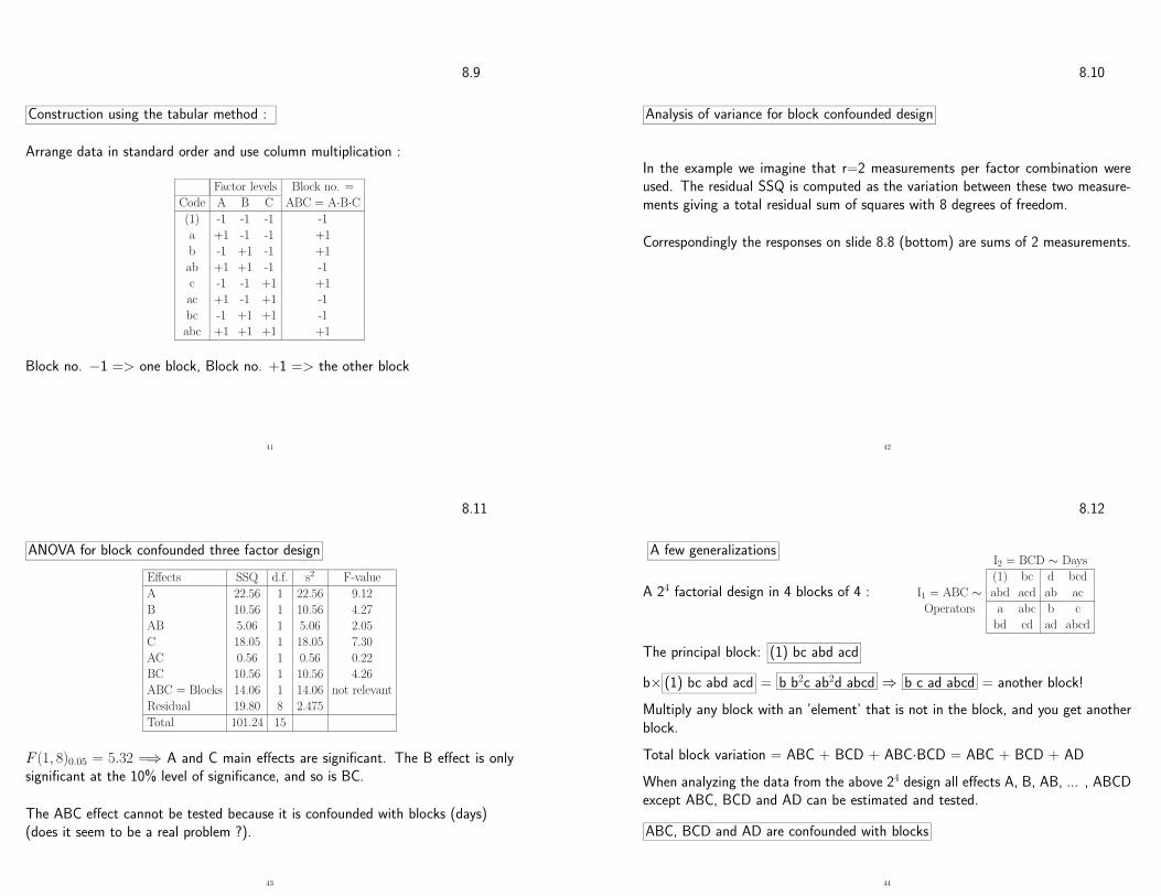
Construction using the tabular method :
Arrange data in standard order and use column multiplication :
Factor levels Block no. =
Code A B C ABC = A·B·C(1) -1 -1 -1 -1
a +1 -1 -1 +1
b -1 +1 -1 +1
ab +1 +1 -1 -1
c -1 -1 +1 +1
ac +1 -1 +1 -1
bc -1 +1 +1 -1
abc +1 +1 +1 +1
Block no. −1 => one block, Block no. +1 => the other block
41
8.10
Analysis of variance for block confounded design
In the example we imagine that r=2 measurements per factor combination wereused. The residual SSQ is computed as the variation between these two measure-ments giving a total residual sum of squares with 8 degrees of freedom.
Correspondingly the responses on slide 8.8 (bottom) are sums of 2 measurements.
42
8.11
ANOVA for block confounded three factor design
Effects SSQ d.f. s2 F-value
A 22.56 1 22.56 9.12
B 10.56 1 10.56 4.27
AB 5.06 1 5.06 2.05
C 18.05 1 18.05 7.30
AC 0.56 1 0.56 0.22
BC 10.56 1 10.56 4.26
ABC = Blocks 14.06 1 14.06 not relevant
Residual 19.80 8 2.475
Total 101.24 15
F (1, 8)0.05 = 5.32 =⇒ A and C main effects are significant. The B effect is onlysignificant at the 10% level of significance, and so is BC.
The ABC effect cannot be tested because it is confounded with blocks (days)(does it seem to be a real problem ?).
43
8.12
A few generalizations
A 24 factorial design in 4 blocks of 4 :
I2 = BCD ∼ Days
(1) bc d bcd
I1 = ABC ∼ abd acd ab ac
Operators a abc b c
bd cd ad abcd
The principal block: (1) bc abd acd
b× (1) bc abd acd = b b2c ab2d abcd ⇒ b c ad abcd = another block!
Multiply any block with an ’element’ that is not in the block, and you get anotherblock.
Total block variation = ABC + BCD + ABC·BCD = ABC + BCD + AD
When analyzing the data from the above 24 design all effects A, B, AB, ... , ABCDexcept ABC, BCD and AD can be estimated and tested.
ABC, BCD and AD are confounded with blocks
44
8.13
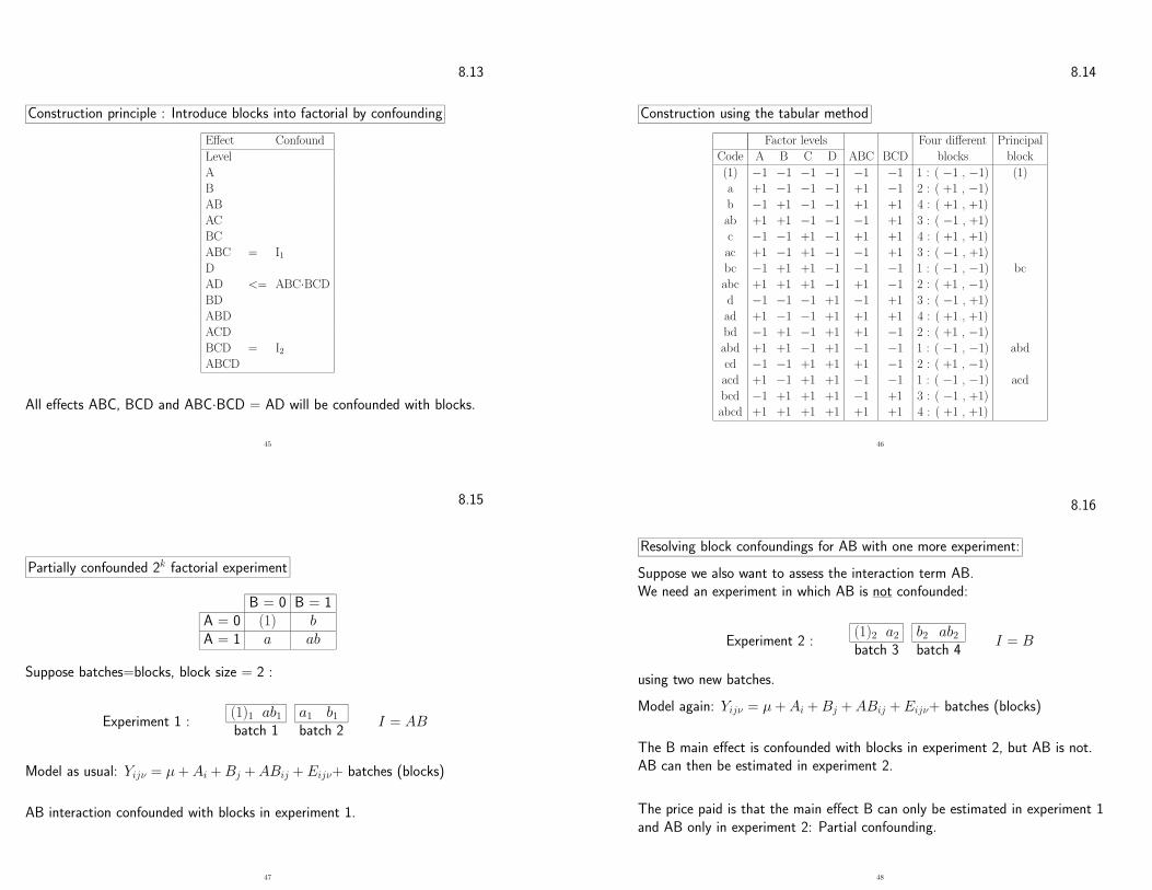
Construction principle : Introduce blocks into factorial by confounding
Effect Confound
Level
A
B
AB
AC
BC
ABC = I1D
AD <= ABC·BCD
BD
ABD
ACD
BCD = I2ABCD
All effects ABC, BCD and ABC·BCD = AD will be confounded with blocks.
45
8.14
Construction using the tabular method
Factor levels Four different Principal
Code A B C D ABC BCD blocks block
(1) −1 −1 −1 −1 −1 −1 1 : ( −1 , −1) (1)
a +1 −1 −1 −1 +1 −1 2 : ( +1 , −1)
b −1 +1 −1 −1 +1 +1 4 : ( +1 , +1)
ab +1 +1 −1 −1 −1 +1 3 : ( −1 , +1)
c −1 −1 +1 −1 +1 +1 4 : ( +1 , +1)
ac +1 −1 +1 −1 −1 +1 3 : ( −1 , +1)
bc −1 +1 +1 −1 −1 −1 1 : ( −1 , −1) bc
abc +1 +1 +1 −1 +1 −1 2 : ( +1 , −1)
d −1 −1 −1 +1 −1 +1 3 : ( −1 , +1)
ad +1 −1 −1 +1 +1 +1 4 : ( +1 , +1)
bd −1 +1 −1 +1 +1 −1 2 : ( +1 , −1)
abd +1 +1 −1 +1 −1 −1 1 : ( −1 , −1) abd
cd −1 −1 +1 +1 +1 −1 2 : ( +1 , −1)
acd +1 −1 +1 +1 −1 −1 1 : ( −1 , −1) acd
bcd −1 +1 +1 +1 −1 +1 3 : ( −1 , +1)
abcd +1 +1 +1 +1 +1 +1 4 : ( +1 , +1)
46
8.15
Partially confounded 2k factorial experiment
B = 0 B = 1A = 0 (1) bA = 1 a ab
Suppose batches=blocks, block size = 2 :
Experiment 1 :(1)1 ab1 a1 b1
batch 1 batch 2I = AB
Model as usual: Yijν = µ + Ai + Bj + ABij + Eijν+ batches (blocks)
AB interaction confounded with blocks in experiment 1.
47
8.16
Resolving block confoundings for AB with one more experiment:
Suppose we also want to assess the interaction term AB.We need an experiment in which AB is not confounded:
Experiment 2 :(1)2 a2 b2 ab2
batch 3 batch 4I = B
using two new batches.
Model again: Yijν = µ + Ai + Bj + ABij + Eijν+ batches (blocks)
The B main effect is confounded with blocks in experiment 2, but AB is not.AB can then be estimated in experiment 2.
The price paid is that the main effect B can only be estimated in experiment 1and AB only in experiment 2: Partial confounding.
48
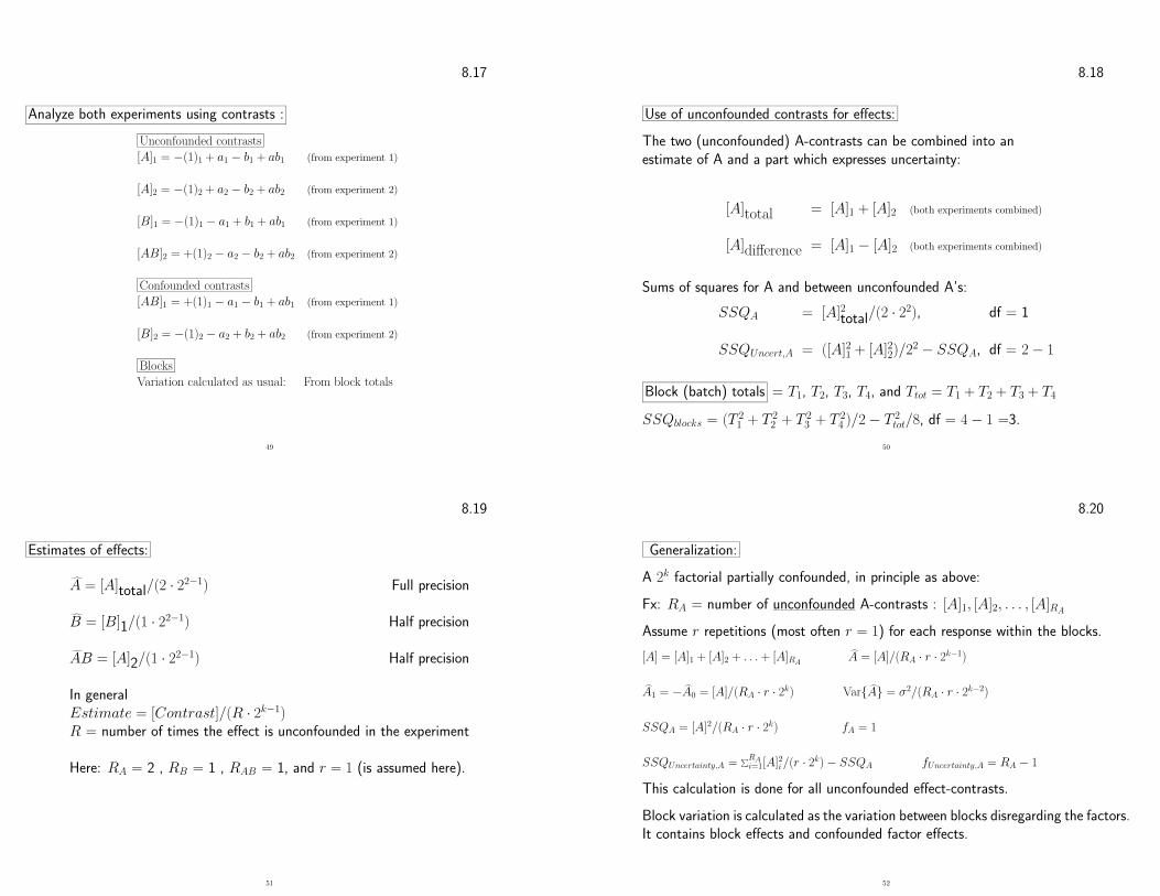
8.17
Analyze both experiments using contrasts :
Unconfounded contrasts
[A]1 = −(1)1 + a1 − b1 + ab1 (from experiment 1)
[A]2 = −(1)2 + a2 − b2 + ab2 (from experiment 2)
[B]1 = −(1)1 − a1 + b1 + ab1 (from experiment 1)
[AB]2 = +(1)2 − a2 − b2 + ab2 (from experiment 2)
Confounded contrasts
[AB]1 = +(1)1 − a1 − b1 + ab1 (from experiment 1)
[B]2 = −(1)2 − a2 + b2 + ab2 (from experiment 2)
Blocks
Variation calculated as usual: From block totals
49
8.18
Use of unconfounded contrasts for effects:
The two (unconfounded) A-contrasts can be combined into anestimate of A and a part which expresses uncertainty:
[A]total = [A]1 + [A]2 (both experiments combined)
[A]difference = [A]1 − [A]2 (both experiments combined)
Sums of squares for A and between unconfounded A’s:
SSQA = [A]2total/(2 · 22), df = 1
SSQUncert,A = ([A]21 + [A]22)/22 − SSQA, df = 2 − 1
Block (batch) totals = T1, T2, T3, T4, and Ttot = T1 + T2 + T3 + T4
SSQblocks = (T 21 + T 2
2 + T 23 + T 2
4 )/2 − T 2tot/8, df = 4 − 1 =3.
50
8.19
Estimates of effects:
A = [A]total/(2 · 22−1) Full precision
B = [B]1/(1 · 22−1) Half precision
AB = [A]2/(1 · 22−1) Half precision
In generalEstimate = [Contrast]/(R · 2k−1)R = number of times the effect is unconfounded in the experiment
Here: RA = 2 , RB = 1 , RAB = 1, and r = 1 (is assumed here).
51
8.20
Generalization:
A 2k factorial partially confounded, in principle as above:
Fx: RA = number of unconfounded A-contrasts : [A]1, [A]2, . . . , [A]RA
Assume r repetitions (most often r = 1) for each response within the blocks.
[A] = [A]1 + [A]2 + . . . + [A]RAA = [A]/(RA · r · 2k−1)
A1 = −A0 = [A]/(RA · r · 2k) Var{A} = σ2/(RA · r · 2k−2)
SSQA = [A]2/(RA · r · 2k) fA = 1
SSQUncertainty,A =∑RA
i=1[A]2i /(r · 2k) − SSQA fUncertainty,A = RA − 1
This calculation is done for all unconfounded effect-contrasts.
Block variation is calculated as the variation between blocks disregarding the factors.It contains block effects and confounded factor effects.
52
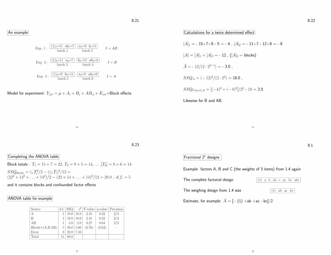
8.21
An example
Exp. 1 :(1)1=15 ab1=7 a1=9 b1=5
batch 1 batch 2I = AB
Exp. 2 :(1)2=11 a2=7 b2=12 ab2=8
batch 3 batch 4I = B
Exp. 3 :(1)3=9 b3=11 a3=8 ab3=6
batch 5 batch 6I = A
Model for experiment: Yijν = µ + Ai + Bj + ABij + Eijν+Block effects
53
8.22
Calculations for a twice determined effect
[A]1 = - 15+7+9 - 5 = - 4 , [A]2 = - 11+7 - 12+8 = - 8
[A] = [A]1 + [A]2 = - 12 , ([A]3 ∼ blocks)
A = - 12/(2 · 22−1) = - 3.0 ,
SSQA = ( - 12)2/(2 · 22) = 18.0 ,
SSQUncert,A = [(−4)2 + ( - 8)2]/22 - 18 = 2.0
Likewise for B and AB.
54
8.23
Completing the ANOVA table
Block totals : T1 = 15 + 7 = 22, T2 = 9 + 5 = 14, ... ,[T6] = 8 + 6 = 14
SSQblocks = ∑i T
2i /2 − (∑
i Ti)2/12 =
(222 + 142 + . . . + 142)/2 − (22 + 14 + . . . + 14)2/12 = 28.0 , d.f. = 5
and it contains blocks and confounded factor effects
ANOVA table for example
Source d.f. SSQ s2 F-value p-value Precision
A 1 18.0 18.0 2.45 0.22 2/3
B 1 18.0 18.0 2.45 0.22 2/3
AB 1 2.0 2.0 0.27 0.64 2/3
Blocks+(A,B,AB) 5 28.0 5.60 (0.76) (0.63) –
Error 3 22.0 7.33
Total 11 88.0
55
9.1
Fractional 2k designs
Example: factors A, B and C (the weights of 3 items) from 1.4 again
The complete factorial design (1) a b ab c ac bc abc
The weighing design from 1.4 was (1) ab ac bc
Estimate, for example: A = [ - (1) +ab +ac - bc]/2
56
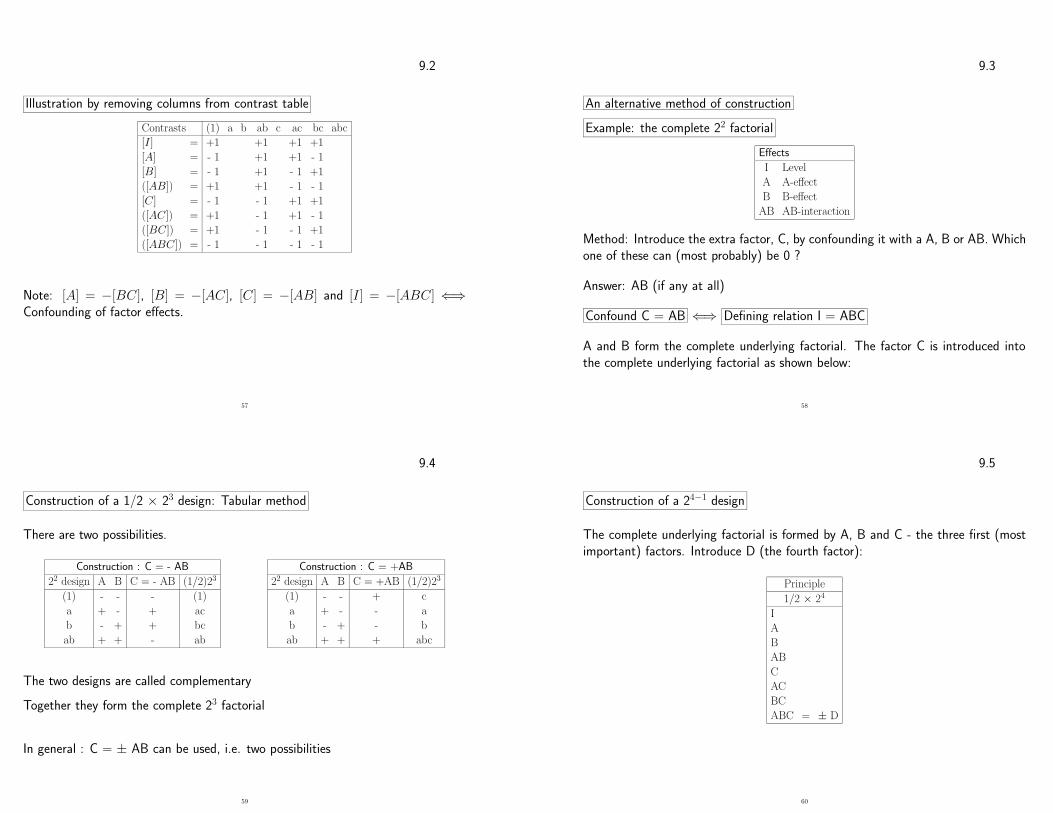
9.2
Illustration by removing columns from contrast table
Contrasts (1) a b ab c ac bc abc
[I ] = +1 +1 +1 +1
[A] = - 1 +1 +1 - 1
[B] = - 1 +1 - 1 +1
([AB]) = +1 +1 - 1 - 1
[C] = - 1 - 1 +1 +1
([AC]) = +1 - 1 +1 - 1
([BC]) = +1 - 1 - 1 +1
([ABC]) = - 1 - 1 - 1 - 1
Note: [A] = −[BC], [B] = −[AC], [C] = −[AB] and [I ] = −[ABC] ⇐⇒Confounding of factor effects.
57
9.3
An alternative method of construction
Example: the complete 22 factorial
Effects
I Level
A A-effect
B B-effect
AB AB-interaction
Method: Introduce the extra factor, C, by confounding it with a A, B or AB. Whichone of these can (most probably) be 0 ?
Answer: AB (if any at all)
Confound C = AB ⇐⇒ Defining relation I = ABC
A and B form the complete underlying factorial. The factor C is introduced intothe complete underlying factorial as shown below:
58
9.4
Construction of a 1/2 × 23 design: Tabular method
There are two possibilities.
Construction : C = - AB
22 design A B C = - AB (1/2)23
(1) - - - (1)
a + - + ac
b - + + bc
ab + + - ab
Construction : C = +AB
22 design A B C = +AB (1/2)23
(1) - - + c
a + - - a
b - + - b
ab + + + abc
The two designs are called complementary
Together they form the complete 23 factorial
In general : C = ± AB can be used, i.e. two possibilities
59
9.5
Construction of a 24−1 design
The complete underlying factorial is formed by A, B and C - the three first (mostimportant) factors. Introduce D (the fourth factor):
Principle
1/2 × 24
I
A
B
AB
C
AC
BC
ABC = ± D
60
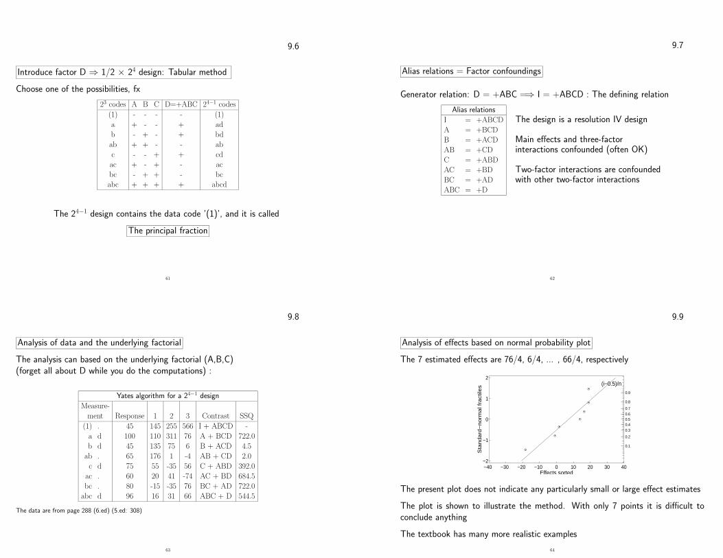
9.6
Introduce factor D ⇒ 1/2 × 24 design: Tabular method
Choose one of the possibilities, fx
23 codes A B C D=+ABC 24−1 codes
(1) - - - - (1)
a + - - + ad
b - + - + bd
ab + + - - ab
c - - + + cd
ac + - + - ac
bc - + + - bc
abc + + + + abcd
The 24−1 design contains the data code ’(1)’, and it is called
The principal fraction
61
9.7
Alias relations = Factor confoundings
Generator relation: D = +ABC =⇒ I = +ABCD : The defining relation
Alias relations
I = +ABCD
A = +BCD
B = +ACD
AB = +CD
C = +ABD
AC = +BD
BC = +AD
ABC = +D
The design is a resolution IV design
Main effects and three-factorinteractions confounded (often OK)
Two-factor interactions are confoundedwith other two-factor interactions
62
9.8
Analysis of data and the underlying factorial
The analysis can based on the underlying factorial (A,B,C)(forget all about D while you do the computations) :
Yates algorithm for a 24−1 design
Measure-
ment Response 1 2 3 Contrast SSQ
(1) . 45 145 255 566 I + ABCD -
a d 100 110 311 76 A + BCD 722.0
b d 45 135 75 6 B + ACD 4.5
ab . 65 176 1 -4 AB + CD 2.0
c d 75 55 -35 56 C + ABD 392.0
ac . 60 20 41 -74 AC + BD 684.5
bc . 80 -15 -35 76 BC + AD 722.0
abc d 96 16 31 66 ABC + D 544.5
The data are from page 288 (6.ed) (5.ed: 308)
63
9.9
Analysis of effects based on normal probability plot
The 7 estimated effects are 76/4, 6/4, ... , 66/4, respectively
−40 −30 −20 −10 0 10 20 30 40−2
−1
0
1
2
Sta
nd
ard
−n
orm
al f
ract
iles
Effects sorted
0.1
0.2
0.30.40.50.60.7
0.8
0.9
(i−0.5)/n
The present plot does not indicate any particularly small or large effect estimates
The plot is shown to illustrate the method. With only 7 points it is difficult toconclude anything
The textbook has many more realistic examples
64
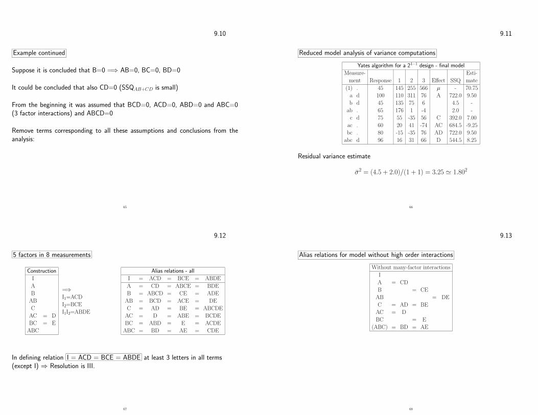
9.10
Example continued
Suppose it is concluded that B=0 =⇒ AB=0, BC=0, BD=0
It could be concluded that also CD=0 (SSQAB+CD is small)
From the beginning it was assumed that BCD=0, ACD=0, ABD=0 and ABC=0(3 factor interactions) and ABCD=0
Remove terms corresponding to all these assumptions and conclusions from theanalysis:
65
9.11
Reduced model analysis of variance computations
Yates algorithm for a 24−1 design - final model
Measure- Esti-
ment Response 1 2 3 Effect SSQ mate
(1) . 45 145 255 566 µ - 70.75
a d 100 110 311 76 A 722.0 9.50
b d 45 135 75 6 4.5 -
ab . 65 176 1 -4 2.0 -
c d 75 55 -35 56 C 392.0 7.00
ac . 60 20 41 -74 AC 684.5 -9.25
bc . 80 -15 -35 76 AD 722.0 9.50
abc d 96 16 31 66 D 544.5 8.25
Residual variance estimate
σ2 = (4.5 + 2.0)/(1 + 1) = 3.25 ' 1.802
66
9.12
5 factors in 8 measurements
Construction
I
A
B
AB
C
AC = D
BC = E
ABC
=⇒I1=ACD
I2=BCE
I1I2=ABDE
Alias relations - all
I = ACD = BCE = ABDE
A = CD = ABCE = BDE
B = ABCD = CE = ADE
AB = BCD = ACE = DE
C = AD = BE = ABCDE
AC = D = ABE = BCDE
BC = ABD = E = ACDE
ABC = BD = AE = CDE
In defining relation I = ACD = BCE = ABDE at least 3 letters in all terms(except I) ⇒ Resolution is III.
67
9.13
Alias relations for model without high order interactions
Without many-factor interactions
I
A = CD
B = CE
AB = DE
C = AD = BE
AC = D
BC = E
(ABC) = BD = AE
68
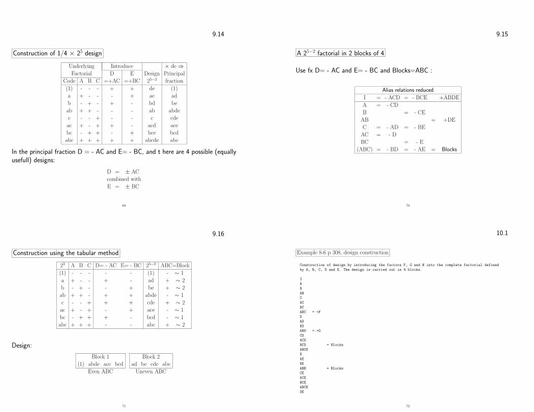
9.14
Construction of 1/4 × 25 design
Underlying Introduce × de ⇒Factorial D E Design Principal
Code A B C =+AC =+BC 25−2 fraction
(1) - - - + + de (1)
a + - - - + ae ad
b - + - + - bd be
ab + + - - - ab abde
c - - + - - c cde
ac + - + + - acd ace
bc - + + - + bce bcd
abc + + + + + abcde abc
In the principal fraction D = - AC and E= - BC, and t here are 4 possible (equallyusefull) designs:
D = ± AC
combined with
E = ± BC
69
9.15
A 25−2 factorial in 2 blocks of 4
Use fx D= - AC and E= - BC and Blocks=ABC :
Alias relations reduced
I = - ACD = - BCE +ABDE
A = - CD
B = - CE
AB = +DE
C = - AD = - BE
AC = - D
BC = - E
(ABC) = - BD = - AE = Blocks
70
9.16
Construction using the tabular method
23 A B C D= - AC E= - BC 25−2 ABC=Block
(1) - - - - - (1) - ∼ 1
a + - - + - ad + ∼ 2
b - + - - + be + ∼ 2
ab + + - + + abde - ∼ 1
c - - + + + cde + ∼ 2
ac + - + - + ace - ∼ 1
bc - + + + - bcd - ∼ 1
abc + + + - - abc + ∼ 2
Design:
Block 1 Block 2
(1) abde ace bcd ad be cde abc
Even ABC Uneven ABC
71
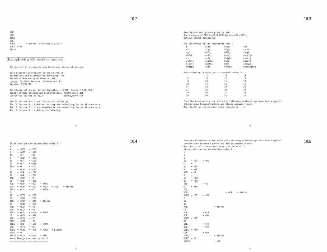
10.1
Example 8-6 p 308, design construction
Construction of design by introducing the factors F, G and H into the complete factorial defined
by A, B, C, D and E. The design is carried out in 4 blocks.
I
A
B
AB
C
AC
BC
ABC = +F
D
AD
BD
ABD = +G
CD
ACD
BCD = Blocks
ABCD
E
AE
BE
ABE = Blocks
CE
ACE
BCE
ABCE
DE
72
10.2
ADE
BDE
ABDE
CDE
ACDE = Blocks ( BCD*ABE = ACDE )
BCDE = +H
ABCDE
Example 8-6 p 308, statistical analyses
Analysis of 2**k complete and fractional factorial designs
This program was prepared by Henrik Spliid
Informatics and Mathematical Modelling (IMM)
Technical University of Denmark (DTU)
Lyngby, DK-2800, Denmark. ([email protected])
Version: 25/08/99
file=Montg_ex8-6.dat, Edited September 1, 2001. Course F-343, DFH.
Input for this problem was read from file Montg_ex9-6.dat
Output was written to file Montg_ex9-6.out
The 10 factors A - J are treated in the design
The 5 factors A - E define the complete underlying factorial structure
The 3 factors F - H are embedded in the underlying factorial structure
The 2 factors I - J define the blocking
73
10.3
Description and options given by user :
Confoundings:(F=ABC,G=ABD,H=BCDE,Blocks=ABE=ACDE),
Options:(LaTeX Dispersion)
The treatments of the experiment were :
h afghj bfgij abi
cfi acgij bcghj abcfh
dgi adfij bdfhj abdgh
cdfgh acdhj bcdij abcdfgi
ej aefg befghi abehij
cefhij aceghi bceg abcefj
deghij adefhi bdef abdegj
cdefgj acde bcdehi abcdefghij
Data ordering in relation to standard order is :
1 2 3 4
5 6 7 8
9 10 11 12
13 14 15 16
17 18 19 20
21 22 23 24
25 26 27 28
29 30 31 32
From the treatments given above the following confoundings have been computed.
Interactions between factors and blocks assumed = zero
Max. factorial interaction order considered = 3
74
10.4Alias relations to interaction order 3 :
*
A = +BCF = +BDG
B = +ACF = +ADG
AB = +CF = +DG
C = +ABF = +DFG
AC = +BF = +EGH
BC = +AF = +DEH
ABC = +F = +CDG
D = +ABG = +CFG
AD = +BG = +EFH
BD = +AG = +CEH
ABD = +CDF = +G
CD = +FG = +BEH
ACD = +BDF = +BCG = +AFG
BCD = +ADF = +ACG = +BFG = +EH = Blocks
ABCD = +DF = +CG = +AEH
E
AE = +DFH = +CGH
BE = +CDH = +FGH
ABE = +CEF = +DEG = Blocks
CE = +BDH = +AGH
ACE = +BEF = +GH
BCE = +AEF = +DH
ABCE = +EF = +ADH = +BGH
DE = +BCH = +AFH
ADE = +BEG = +FH
BDE = +AEG = +CH
ABDE = +EG = +ACH = +BFH
CDE = +EFG = +BH
ACDE = +ABH = +CFH = +DGH = Blocks
BCDE = +H
ABCDE = +DEF = +CEG = +AH
Note: Design has resolution IV
==============================
75
10.5From the treatments given above the following confoundings have been computed.
Interactions between factors and blocks assumed = zero
Max. factorial interaction order considered = 2
Alias relations to interaction order 2 :
*
A
B
AB = +CF = +DG
C =
AC = +BF
BC = +AF
ABC = +F
D =
AD = +BG
BD = +AG
ABD = +G
CD = +FG
ACD
BCD = +EH = Blocks
ABCD = +DF = +CG
E
AE
BE
ABE = Blocks
CE
ACE = +GH
BCE = +DH
ABCE = +EF
DE
ADE = +FH
BDE = +CH
ABDE = +EG
CDE = +BH
ACDE = Blocks
BCDE = +H
ABCDE = +AH
76
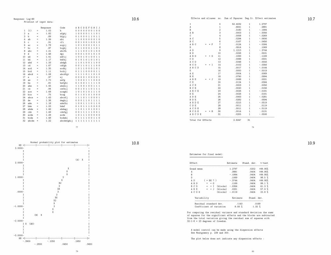
10.6Response: Log-SD
Printout of input data:
Response Code A B C D E F G H I J
1 (1) = 1.02 h 0 0 0 0 0 0 0 1 0 0
2 a = 1.82 afghj 1 0 0 0 0 1 1 1 0 1
3 b = .89 bfgij 0 1 0 0 0 1 1 0 1 1
4 ab = 1.39 abi 1 1 0 0 0 0 0 0 1 0
5 c = .91 cfi 0 0 1 0 0 1 0 0 1 0
6 ac = 1.78 acgij 1 0 1 0 0 0 1 0 1 1
7 bc = .87 bcghj 0 1 1 0 0 0 1 1 0 1
8 abc = 1.21 abcfh 1 1 1 0 0 1 0 1 0 0
9 d = 1.48 dgi 0 0 0 1 0 0 1 0 1 0
10 ad = 1.41 adfij 1 0 0 1 0 1 0 0 1 1
11 bd = 1.17 bdfhj 0 1 0 1 0 1 0 1 0 1
12 abd = 1.33 abdgh 1 1 0 1 0 0 1 1 0 0
13 cd = 1.67 cdfgh 0 0 1 1 0 1 1 1 0 0
14 acd = 1.35 acdhj 1 0 1 1 0 0 0 1 0 1
15 bcd = 1.11 bcdij 0 1 1 1 0 0 0 0 1 1
16 abcd = 1.08 abcdfgi 1 1 1 1 0 1 1 0 1 0
17 e = .97 ej 0 0 0 0 1 0 0 0 0 1
18 ae = 1.70 aefg 1 0 0 0 1 1 1 0 0 0
19 be = .81 befghi 0 1 0 0 1 1 1 1 1 0
20 abe = 1.45 abehij 1 1 0 0 1 0 0 1 1 1
21 ce = .94 cefhij 0 0 1 0 1 1 0 1 1 1
22 ace = 1.68 aceghi 1 0 1 0 1 0 1 1 1 0
23 bce = .75 bceg 0 1 1 0 1 0 1 0 0 0
24 abce = 1.43 abcefj 1 1 1 0 1 1 0 0 0 1
25 de = 1.38 deghij 0 0 0 1 1 0 1 1 1 1
26 ade = 1.18 adefhi 1 0 0 1 1 1 0 1 1 0
27 bde = 1.23 bdef 0 1 0 1 1 1 0 0 0 0
28 abde = 1.46 abdegj 1 1 0 1 1 0 1 0 0 1
29 cde = 1.49 cdefgj 0 0 1 1 1 1 1 0 0 1
30 acde = 1.29 acde 1 0 1 1 1 0 0 0 0 0
31 bcde = 1.48 bcdehi 0 1 1 1 1 0 0 1 1 0
32 abcde = 1.22 abcdefghij 1 1 1 1 1 1 1 1 1 1
77
10.7Effects and aliases no. Sum of Squares Deg.fr. Effect estimates
* 0 52.4032 1 1.2797
A 1 .6641 1 .2881
B 2 .3180 1 -.1994
A B 3 .0003 1 -.0056
C 4 .0058 1 -.0269
A C 5 .0294 1 -.0606
B C 6 .0167 1 -.0456
A B C = + F 7 .0124 1 -.0394
D 8 .0914 1 .1069
A D 9 1.1213 1 -.3744
B D 10 .0226 1 .0531
A B D = + G 11 .1093 1 .1169
C D 12 .0088 1 .0331
A C D 13 .0248 1 -.0556
B C D = + I 14 .0102 1 -.0356
A B C D 15 .0017 1 -.0144
E 16 .0000 1 -.0019
A E 17 .0004 1 .0069
B E 18 .0790 1 .0994
A B E = + J 19 .0088 1 .0331
C E 20 .0124 1 .0394
A C E 21 .0003 1 .0056
B C E 22 .0020 1 .0156
A B C E 23 .0026 1 -.0181
D E 24 .0026 1 .0181
A D E 25 .0063 1 -.0281
B D E 26 .0282 1 .0594
A B D E 27 .0215 1 -.0519
C D E 28 .0011 1 .0119
A C D E 29 .0011 1 -.0119
B C D E = + H 30 .0014 1 .0131
A B C D E 31 .0205 1 -.0506
------------------------------------------------------------------
Total for Effects 2.6247 31
78
10.8Normal probability plot for estimates
HS +I--------I---------I---------I---------I---------I+
3.0000- -
I I
I I
I I
I (A) X I
2.0000- -
I I
I X I
I X I
I X I
1.0000- 2 -
I X I
I X2 I
I 2 I
I XX I
.0000- 3 -
I 2 I
I XX I
I X2 I
I X I
-1.0000- 2 -
I X I
I X I
I (B) X I
I I
-2.0000- -
I X (AD) I
I I
I I
I I
-3.0000- -
HS +I--------I---------I---------I---------I---------I+
-.3900 -.1050 .1950
-.2550 .0450 .3450
79
10.9
Estimates for final model:
==========================
Effect Estimate Stand. dev. t-test
-------------------------------------------------------------
Grand mean 1.2797 .0202 >99.95%
A .2881 .0404 >99.95%
B -.1994 .0404 >99.95%
D .1069 .0404 98.5 %
A D ( = BG ? ) -.3744 .0404 >99.95%
A B D = + G .1169 .0404 99.1 %
B C D = + I (blocks) -.0356 .0404 61.3 %
A B E = + J (blocks) .0331 .0404 57.9 %
A C D E (blocks) -.0119 .0404 22.8 %
Variability Estimate Stand. dev.
-----------------------------------------------------
Residual standard dev. .1143 .0169
Coefficient of variation 8.93 % 1.32 %
For computing the residual variance and standard deviation the sums
of squares for the significant effects and the blocks are subtracted
from the total variation giving the residual sum of squares with
32-1-8 = 23 degrees of freedom.
A model control can be made using the dispersion effects
See Montgomery p. 239 and 300.
The plot below does not indicate any dispersion effects :
80
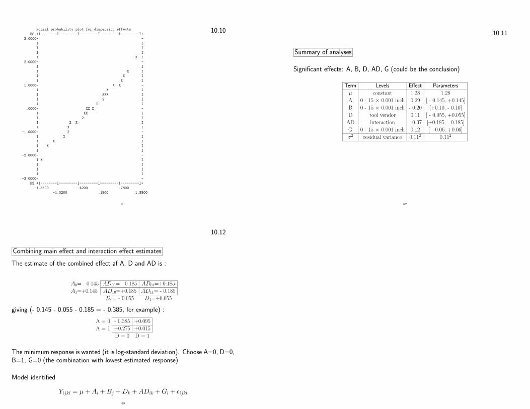
10.10Normal probability plot for dispersion effects
HS +I--------I---------I---------I---------I---------I+
3.0000- -
I I
I I
I I
I X I
2.0000- -
I I
I X I
I X I
I X I
1.0000- X X -
I X I
I XXX I
I 2 I
I 2 I
.0000- XX X -
I XX I
I 2 I
I 2 X I
I X I
-1.0000- 2 -
I X I
I X I
I X I
I I
-2.0000- -
I X I
I I
I I
I I
-3.0000- -
HS +I--------I---------I---------I---------I---------I+
-1.5600 -.4200 .7800
-1.0200 .1800 1.3800
81
10.11
Summary of analyses
Significant effects: A, B, D, AD, G (could be the conclusion)
Term Levels Effect Parameters
µ constant 1.28 1.28
A 0 - 15 × 0.001 inch 0.29 [ - 0.145, +0.145]
B 0 - 15 × 0.001 inch - 0.20 [+0.10, - 0.10]
D tool vendor 0.11 [ - 0.055, +0.055]
AD interaction - 0.37 [+0.185, - 0.185]
G 0 - 15 × 0.001 inch 0.12 [ - 0.06, +0.06]
σ2 residual variance 0.112 0.112
82
10.12
Combining main effect and interaction effect estimates
The estimate of the combined effect af A, D and AD is :
A0= - 0.145 AD00= - 0.185 AD01=+0.185
A1=+0.145 AD10=+0.185 AD11= - 0.185
D0= - 0.055 D1=+0.055
giving (- 0.145 - 0.055 - 0.185 = - 0.385, for example) :
A = 0 - 0.385 +0.095
A = 1 +0.275 +0.015
D = 0 D = 1
The minimum response is wanted (it is log-standard deviation). Choose A=0, D=0,B=1, G=0 (the combination with lowest estimated response)
Model identified
Yijkl = µ + Ai + Bj + Dk + ADik + Gl + εijkl
83