Statistical downscaling in European mountains

CLIMATE RESEARCHClim Res

Vol. 26: 97–112, 2004 Published May 25

1. INTRODUCTION

Mountain environments support a substantial pro-portion of the human population, contain a wide rangeof ecological variability and are the source of much ofthe world’s water systems. Climatic change at high ele-vation sites can be dramatically amplified by feedbackeffects associated with the albedos of snow and ice.Consequently there is a pressing need to understandthe impacts of interannual variability and extremeclimate conditions on our mountain systems. To exam-ine climatic change over the last century, long timeseries of meteorological observations are required.These records must be homogeneous such that varia-tions are purely a result of the weather and climate andnot caused by factors such as changes in instrumenta-

tion, instrument drift, urban warming or relocation ofstation. In many parts of the world, such high qualityrecords are sparsely distributed. In recent years gen-eral circulation models (GCMs), constrained by histor-ical meteorological records, have been run to produceconsistent simulations of the state of the atmosphereover the past 4 decades. These assimilations areknown as reanalysis models. One very useful aspect ofthe reanalysis modelling work is that it has the abilityto transport information from data-rich to data-sparseregions. However, while GCMs can simulate large-scale upper air circulation fairly accurately, they arepoor at reproducing surface variables on regional andlocal scales (Grotch & MacCracken 1991). Therefore,to examine climate at a sub-grid scale it is necessary torelate the gridded reanalysis data to an observed

© Inter-Research 2004 · www.int-res.com*Email: [email protected]

Statistical downscaling in European mountains:verification of reconstructed air temperature

Helen Kettle*, Roy Thompson

School of GeoSciences, University of Edinburgh, West Mains Road, Edinburgh EH9 3JW, UK

ABSTRACT: General circulation models constrained by past meteorological records have been run aspart of a major community effort, using datasets from 1958 to the present date, to produce consistentgridded atmospheric databases known as reanalysis data. We derive linear regression models totransfer reanalysis gridded data to high elevation weather stations in Europe using daily observationsfrom 1994 to 2001. The models are then used to reconstruct daily mean, minimum and maximum airtemperatures since 1958 at the weather stations. The regression models use principal components ofreanalysis temperature and pressure variables in addition to local (nearest grid point) temperatureand pressure variables. An all-subsets regression technique in conjunction with cross validation isused to find the best model. The accuracy of the approach is verified using observed monthly datafrom 1980 to 1990 at 29 stations, and monthly data since 1958 at 8 stations. The verification resultsindicate that retrodiction to 1980 is good at all stations. However, validation at 3 alpine stations showslarge differences between observed and reconstructed temperatures prior to 1970. Nevertheless, thebasic spatio-temporal warming pattern we reconstruct for the European mountains has many simi-larities to that for the European ‘lowlands’. We find regional climatic trends for the period 1958to 2001 of typically 0.7°C per 100 yr for minimum temperatures and twice that for maximum temper-atures. These trends are probably underestimated. Our reconstructions suggest that there has beenan increase in the diurnal temperature range in European mountains in addition to the overallwarming.

KEY WORDS: Downscaling · Climate · Mountains · ‘Reanalysis data’

Resale or republication not permitted without written consent of the publisher

Clim Res 26: 97–112, 2004

meteorological variable at a specific location, a processknown as downscaling. Downscaling techniques canbe summarised into 4 categories: regression methods;weather pattern-based methods; stochastic weathergenerators; and limited area modelling (Wilby &Wigley 1997). In this work we use regression methodsto downscale air temperature. This involves the con-struction of a linear regression model relating reanaly-sis variables to observed surface air temperatures.Reconstruction of an observed variable outside itsobservation period relies on the assumption that therelationship between the large-scale circulation andthe local climate does not change over time. As with allregression models, application of the model is limitedby the range of data used in its construction. Ifobserved data covering the full time period of thereanalysis data were used to construct the model, thenit would be a robust (because it is built over manydecades), but essentially redundant model as it is notproviding any new information. To make real use ofthe reanalysis data we need to know whether modelsbased on relatively short-term surface records can beused to reconstruct surface temperatures over previousdecades.

Correlations between air temperatures recorded atseveral mountain weather stations in a given regionare higher than correlations between air temperaturesrecorded at several low-lying stations in the sameregion (Weber et al. 1997), implying that mountain sta-tions are less subject to local effects. Meteorologicalvariables recorded at mountain stations present anideal opportunity for examining climatic change asthey are generally far from large cities and free fromthe warming associated with urbanisation. There isalso evidence that the amplitude of temperaturechange this century at many high elevation sites isgreater than the observed global change, implyingthat impacts of future climatic change will be greater athigh elevations (Beniston et al. 1997). By reconstruct-ing daily data at these locations it is possible to studychanges in climate trends, variability and extremes.

The response of the local climate to the large-scaleclimate at a particular weather station can differ de-pending on the siting of the station. For example, if thestation is on the side of a hill, the orientation of theslope may affect cloud cover and snow lie; stations setat the bottom of high valleys may experience tempera-ture inversions; glaciers generate pronounced localeffects and conditions at stations on high plateaus willdiffer from those on mountain tops. Small-scale influ-ences such as local convective activity, orography, veg-etation and soil characteristics can influence local windsystems, snow cover or energy exchange with the at-mosphere, thus uncoupling the variability of individualweather elements from the large-scale circulation.

However, regional topography and land use at eachstation should be implicitly incorporated in the individ-ual linear regression models used for downscaling.Due to the lack of human interference at mountainstations such factors should not have changed over thelast 50 yr.

The aim of this study is to answer the following ques-tions regarding downscaling in European mountains:

(1) Is there a difference in the accuracy of down-scaled minimum, maximum and mean daily air tem-peratures?

(2) Is there a seasonal difference in downscalingaccuracy?

(3) Are temporal and spatial structures in the tem-perature series correctly downscaled?

(4) Which reanalysis variables are the most impor-tant predictors?

(5) Can we accurately reconstruct air temperaturesbetween 1980 and 1990?

(6) Can we accurately reconstruct air temperaturesback to 1958?

(7) How accurate are the long-term climatic trendsderived from reconstructed temperatures?

(8) How do the reconstructed trends compare withestablished climate trends?

2. DATASETS

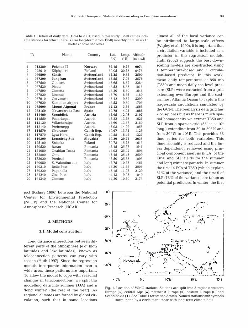
In this work we focus on European mountain obser-vatories where daily air temperatures since 1994(which are used to build the regression models) andmean monthly temperatures from 1980 to 1990 (whichare used for verification of the models) are available.The daily data provide daily minimum, maximum andmean temperatures. All of the stations used are well-maintained, quality-controlled World MeteorologicalOrganisation (WMO) sites situated 1000 m above sealevel (a.s.l.) in central and southern Europe, and above700 m in Scandinavia. The height constraint is lower inScandinavia because at this more northerly latitude,surface temperatures are lower so that conditions atthese lower elevations are similar to those in the highAlps. To help ensure the regression models are fairlyrobust and not overfitted, the additional constraint thatat least 5 yr of daily data must be available since 1994was imposed. Details and locations of the 29 stationsthat satisfied our constraints are given in Table 1 andFig. 1. For 8 of these stations, namely Sonnblick (Aus-tria), Jungfrau and Säntis (Switzerland), Lomnicky Stit(Slovakia), Fokstua II (Norway), Mount Aigoual(France), Churanov (Czech Republic) and Navacer-rada Pass (Spain) monthly data extend back severaldecades. The reanalysis data were obtained from thelarge assimilation datasets produced by the joint pro-

98

Kettle & Thompson: Statistical downscaling in European mountains

ject (Kalnay 1996) between the NationalCenter for Environmental Prediction(NCEP) and the National Center forAtmospheric Research (NCAR).

3. METHODS

3.1. Model construction

Long distance interactions between dif-ferent parts of the atmosphere (e.g. highlatitudes and low latitudes), known asteleconnection patterns, can vary withseason (Huth 1997). Since the regressionmodels incorporate information over awide area, these patterns are important.To allow the model to cope with seasonalchanges in teleconnections, we split themodelling data into summer (JJA) and a‘long winter’ (the rest of the year). Asregional climates are forced by global cir-culation, such that in some locations

almost all of the local variance canbe attributed to large-scale effects(Wigley et al. 1990), it is important thata circulation variable is included as apredictor in the regression models.Huth (2002) suggests the best down-scaling models are constructed using1 temperature-based and 1 circula-tion-based predictor. In this work,mean daily temperatures at 850 mb(T850) and mean daily sea level pres-sure (SLP) were extracted from a gridextending over Europe and the east-ernmost Atlantic Ocean to capture thelarge-scale circulations simulated bythe GCM. The reanalysis data grid has2.5° squares but as there is much spa-tial homogeneity we extract T850 andSLP from a sparser grid (5° lat. × 10°long.) extending from 30 to 80° N andfrom 30° W to 40° E. This provides 88time series for both variables. Thisdimensionality is reduced and the lin-ear dependency removed using prin-cipal component analysis (PCA) of theT850 and SLP fields for the summerand long winter separately. In summerthe first 14 PCs of T850 (which explain81% of the variance) and the first 9 ofSLP (78% of the variance) are taken aspotential predictors. In winter, the first

99

Fig. 1. Location of WMO stations. Stations are split into 5 regions: westernEurope (n), central Alps (M), northeast Europe (e), eastern Europe (s) andScandinavia (f). See Table 1 for station details. Named stations with symbols

surrounded by a circle mark those with long-term climate data

ID Name Country Lat. Long. Altitude(° N) (° E) (m a.s.l)

1 012380 Fokstua II Norway 62.15 9.28 09742 028010 Kilpisjarvi Finland 69.05 20.78 04763 066800 Säntis Switzerland 47.25 9.35 25004 067300 Jungfrau Switzerland 46.55 7.98 35765 067500 Guetsch Switzerland 46.65 8.62 22846 067530 Piotta Switzerland 46.52 8.68 10167 067590 Cimetta Switzerland 46.20 8.80 16488 067820 Disentis Switzerland 46.70 8.85 11809 067910 Corvatsch Switzerland 46.42 9.82 329910 067920 Samedan airport Switzerland 46.53 9.89 170611 075600 Mount Aigoual France 44.12 3.58 156512 082150 Navacerrada Pass Spain 40.78 –4.02 188813 111460 Sonnblick Austria 47.05 12.95 310714 111550 Feuerkogel Austria 47.82 13.73 162115 112120 Villacheralpe Austria 46.60 13.67 216016 112140 Preitenegg Austria 46.93 14.92 105517 114570 Churanov Czech Rep. 49.07 13.62 112618 117870 Lysa Hora Czech Rep. 49.55 18.45 132719 119300 Lomnicky Stit Slovakia 49.20 20.22 263520 125100 Sniezka Poland 50.73 15.73 161321 150520 Rarau Romania 47.45 25.57 154122 151080 Ceahlau Toaca Romania 46.93 25.92 189823 152800 Omu Romania 45.45 25.45 250924 153020 Predeal Romania 45.50 25.58 109325 160080 S. Valentino alla Italy 45.75 10.53 146126 160210 Rolle Pass Italy 46.30 11.78 200627 160220 Paganella Italy 46.15 11.03 212928 161240 Cisa Pass Italy 44.43 9.93 104029 161340 Cimone Italy 44.20 10.70 2173

Table 1. Details of daily data (1994 to 2001) used in this study. Bold values indi-cate stations for which there is also long-term (from 1958) monthly data. m a.s.l.:

metres above sea level

Clim Res 26: 97–112, 2004

13 (89% of the variance) of T850 and first 10 (88% ofthe variance) of SLP are retained. Although it is desir-able to retain more principal components, practicalrestraints on computing time limit the number ofpotential predictors. In addition to these circulationvariables, at each surface site considered, we also usethe following data from the nearest reanalysis gridpoint: air temperatures at pressure levels 200, 500 and850 mb (T200, T500 and T850, respectively); minimum,maximum and mean surface temperatures and SLP.These combined with the PCA scores give a total of 30potential predictors.

The downscaling models were derived by followinga procedure that can be broken down into 6 steps:

Step 1. All time series were split into summer andlong winter components. Steps 2 to 5 were thenapplied to data from the 2 seasons separately.

Step 2. All time series were normalised by subtract-ing the mean and dividing by the standard deviationfollowing Huth (1999).

Step 3. A process known as ‘leaps and bounds’ or ‘allsubsets regression’ was used to choose the best down-scaling model in terms of cross validation root meansquared error (RMSE). For m predictors this methodfits all 2m possible subsets of predictors to the predic-tand. The fit criterion is Mallow’s Cp:

(1)

where n is number of observations, RSS is the sum ofsquared errors, MSE is the residual mean squareerror and p is the number of model parameters. Amodel that fits well will have a computed Cp valueclose to p. If there are several, the model with thesmallest value of Cp is chosen. For each size of sub-set, the best subset of predictors (in terms of Cp) wasretained leaving 30 possible subsets (models) tochoose between.

Step 4. The best subset size was found using crossvalidation. Data from 1 yr are set aside from themodel building process. The model is constructedusing only the remaining data and then used to pre-dict the year of data that had been held aside. Thisvalidation process is repeated for every year forwhich there are data. Thus for 8 yr of data there are 8cross validation models built per subset size. Theminimum of the average RMSE values over all of thevalidation periods is used to choose the best subsetsize.

Step 5. The final fit is produced using all of the data(no data set aside) with the number of predictorsdefined by the best subset size in the cross validationof Step 4. The best model (in terms of Cp) for this num-ber of predictors was derived and used to reconstructdaily temperatures since 1958.

Step 6. The 2 reconstructions of summers/long win-ters were then combined to provide daily temperaturesfrom 1 January 1958 to 31 December 2001.

This whole procedure (Steps 1 through 6) wasrepeated separately for the daily minimum, maximumand mean air temperature at each of the 29 stations.

Although the yearly cycle is not explicitly removedfrom the data, it is captured in the first principal com-ponents of the temperature and pressure datasets. It isthus handled naturally as an integral part of our mod-elling procedure.

3.2. Cross validation statistics

Average cross validation statistics were calculatedfor the best summer and winter models so that therewere 2 RMSE, mean absolute error (MAE), bias andskill values for each station. The MAE shows the aver-age error in the prediction without the disproportion-ate weighting the RMSE gives to occasional very largeerrors. The bias, which is the mean prediction error, ispositive if the model is systematically overestimatingair temperatures (and vice versa). The forecast skill isdefined as:

(2)

by Lorenz (1956) in which xi and x̂i are the actual andestimated air temperatures in the verification seasonfor each data point i, and x -c is the mean of the actualair temperatures in the calibration seasons. The closerthe skill is to 100% the better the prediction.

4. EVALUATION OF MODELS

4.1. Predictors

At each station we have 30 variables (predictors)derived from the reanalysis assimilation datasets thatcan be used for downscaling. Some of these predictorswill be used more frequently than others. To establishwhich are the important predictors for downscaling inEuropean mountains, the number of stations usingeach predictor was calculated. The results, in Table 2,show that when downscaling to surface mean, maxi-mum and minimum daily air temperatures the T850 atthe local reanalysis grid point is the most used vari-able with the 1 exception of the minimum daily tem-perature in winter, which uses the local surface mini-mum temperature. In general, the summer models uselocal grid point data rather than the principal compo-nents of T850 and SLP. In contrast the winter modelsalways select at least one of the principal component

skill

c

= × −−−

∑∑100 1 0

2

2% .

( ˆ )

( )

x x

x xi i

i

C n pp = − −

RSSMSE

( )2

100


scores to be included in the top 3 predictors. This mayreflect the increased strength of teleconnections inwinter. The summer models typically require only halfthe number of predictors used by the winter models,which could be a function of the relatively small num-ber of data points available in summer (3 mo com-pared to the 9 mo used in winter). Since all the mod-els are thoroughly cross validated, there is no grossover-fitting even when a large number of predictorsare retained.

4.2. Cross validation statistics

As described in Section 3.1, part of the model build-ing process at each station involves cross validation.This allows the predictive accuracy of the model to beassessed without reducing the amount of data avail-able for deriving the final model. The error statistics forthe omitted seasons are averaged separately, provid-ing summer and winter cross validation statistics ateach station. Table 3 summarises these results for dailymean, minimum and maximum temperatures aver-aged over all of the stations. The cross validation sta-tistics quoted for both models are averaged over thesummer and winter models with a time weighting of3/12 for summer and 9/12 for winter. The MAE andRMSE values indicate that the summer mean dailytemperature and the winter daily maximum tempera-ture are the most and least accurately downscaled vari-

ables respectively. In general, the skill of the down-scaling appears much better in summer than winter.This is possibly because there is much greater naturalvariability in the winter months. For example, averagestandard deviations at Jungfrau mountain since 1994are 3.1°C in summer and 4.4°C in winter. Because thecross validation skill takes into account the deviation ofthe observed data from its mean in the calibrationperiod, it is possible for a high downscaling skill to beassociated with a high RMSE (e.g. maximum tempera-tures in the summer model, Table 3). In our work, thecross validation skill cannot be used to comparebetween the summer and long winter models as theannual cycle in the data distorts the relative values.The skill is only useful for comparing between stations,but the RMSE can be used to compare betweenseasons.

4.3. Temporal and spatial structure

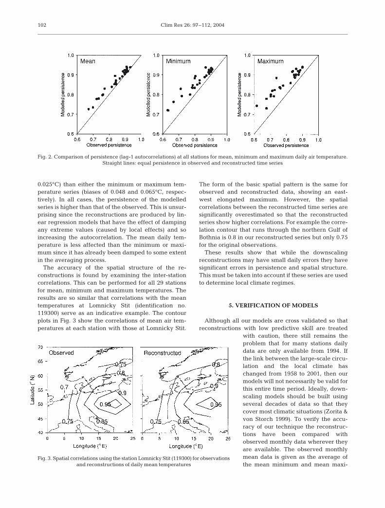
The accuracy of the temporal structure of the recon-structions is found by comparing the persistence (lag-1autocorrelation) of the reconstructions with that of theobserved time series. The persistence of the recon-structions is calculated over the time period of the sur-face observations. The results for the mean, maximumand minimum daily temperatures are shown in Fig. 2.The mean daily temperature reconstructions have atemporal structure closer to the observed series (bias

101

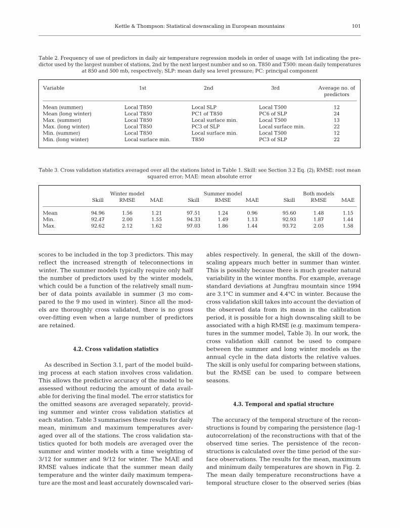
Variable 1st 2nd 3rd Average no. ofpredictors

Mean (summer) Local T850 Local SLP Local T500 12Mean (long winter) Local T850 PC1 of T850 PC6 of SLP 24Max. (summer) Local T850 Local surface min. Local T500 13Max. (long winter) Local T850 PC3 of SLP Local surface min. 22Min. (summer) Local T850 Local surface min. Local T500 12Min. (long winter) Local surface min. T850 PC3 of SLP 22

Table 2. Frequency of use of predictors in daily air temperature regression models in order of usage with 1st indicating the pre-dictor used by the largest number of stations, 2nd by the next largest number and so on. T850 and T500: mean daily temperatures

at 850 and 500 mb, respectively; SLP: mean daily sea level pressure; PC: principal component

Winter model Summer model Both modelsSkill RMSE MAE Skill RMSE MAE Skill RMSE MAE

Mean 94.96 1.56 1.21 97.51 1.24 0.96 95.60 1.48 1.15Min. 92.47 2.00 1.55 94.33 1.49 1.13 92.93 1.87 1.44Max. 92.62 2.12 1.62 97.03 1.86 1.44 93.72 2.05 1.58

Table 3. Cross validation statistics averaged over all the stations listed in Table 1. Skill: see Section 3.2 Eq. (2); RMSE: root mean squared error; MAE: mean absolute error

Clim Res 26: 97–112, 2004

0.025°C) than either the minimum or maximum tem-perature series (biases of 0.048 and 0.065°C, respec-tively). In all cases, the persistence of the modelledseries is higher than that of the observed. This is unsur-prising since the reconstructions are produced by lin-ear regression models that have the effect of dampingany extreme values (caused by local effects) and soincreasing the autocorrelation. The mean daily tem-perature is less affected than the minimum or maxi-mum since it has already been damped to some extentin the averaging process.

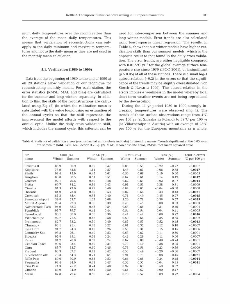
The accuracy of the spatial structure of the re-constructions is found by examining the inter-stationcorrelations. This can be performed for all 29 stationsfor mean, minimum and maximum temperatures. Theresults are so similar that correlations with the meantemperatures at Lomnicky Stit (identification no.119300) serve as an indicative example. The contourplots in Fig. 3 show the correlations of mean air tem-peratures at each station with those at Lomnicky Stit.

The form of the basic spatial pattern is the same forobserved and reconstructed data, showing an east-west elongated maximum. However, the spatialcorrelations between the reconstructed time series aresignificantly overestimated so that the reconstructedseries show higher correlations. For example the corre-lation contour that runs through the northern Gulf ofBothnia is 0.8 in our reconstructed series but only 0.75for the original observations.

These results show that while the downscalingreconstructions may have small daily errors they havesignificant errors in persistence and spatial structure.This must be taken into account if these series are usedto determine local climate regimes.

5. VERIFICATION OF MODELS

Although all our models are cross validated so thatreconstructions with low predictive skill are treated

with caution, there still remains theproblem that for many stations dailydata are only available from 1994. Ifthe link between the large-scale circu-lation and the local climate haschanged from 1958 to 2001, then ourmodels will not necessarily be valid forthis entire time period. Ideally, down-scaling models should be built usingseveral decades of data so that theycover most climatic situations (Zorita &von Storch 1999). To verify the accu-racy of our technique the reconstruc-tions have been compared withobserved monthly data wherever theyare available. The observed monthlymean data is given as the average ofthe mean minimum and mean maxi-

102

Fig. 2. Comparison of persistence (lag-1 autocorrelations) at all stations for mean, minimum and maximum daily air temperature. Straight lines: equal persistence in observed and reconstructed time series

Fig. 3. Spatial correlations using the station Lomnicky Stit (119300) for observations and reconstructions of daily mean temperatures


mum daily temperatures over the month rather thanthe average of the mean daily temperatures. Thismeans that verification of reconstructions can onlyapply to the daily minimum and maximum tempera-tures and not to the daily mean as they are not used inthe monthly mean calculation.

5.1. Verification (1980 to 1990)

Data from the beginning of 1980 to the end of 1990 atall 29 stations allow validation of our technique forreconstructing monthly means. For each station, theerror statistics (RMSE, MAE and bias) are calculatedfor the summer and long winters separately. In addi-tion to this, the skills of the reconstructions are calcu-lated using Eq. (2) (in which the calibration mean issubstituted with the value found using an estimation ofthe annual cycle) so that the skill represents theimprovement the model affords with respect to theannual cycle. Unlike the daily cross validation skill,which includes the annual cycle, this criterion can be

used for intercomparison between the summer andlong winter models. Error trends are also calculatedusing least squares linear regression. The results, inTable 4, show that our winter models have higher ver-ification skills than our summer models, which is theopposite result to that found in the daily cross valida-tion. The error trends, are either negligible comparedwith 0.01.5°C yr–1 for the global average surface tem-perature rise since 1979 (IPCC 2001), or insignificant(p > 0.05) at all of these stations. There is a small lag-1autocorrelation (~0.2) in the errors so that the signifi-cance of the trends may be slightly overestimated (vonStorch & Navarra 1999). The autocorrelation in theerrors implies a weakness in the model whereby localshort-term weather events are not being reproducedby the downscaling.

During the 11 yr period 1980 to 1990 strongly in-creasing temperatures were observed (Fig 4). Thetrends of these surface observations range from 4°Cper 100 yr (at Sniezka in Poland) to 39°C per 100 yr(at Villacheralpe in Austria) with an average of 23°Cper 100 yr for the European mountains as a whole.

103

Stn Skill (%) MAE (°C) RMSE (°C) Bias (°C) Trend in errorsname Winter Summer Winter Summer Winter Summer Winter Summer (°C per 100 yr)

Fokstua II 85.9 80.9 0.69 0.47 0.85 0.59 –0.22 –0.27 –0.0007Kilpisjarvi 75.9 82.8 1.11 0.57 1.45 0.67 0.66 0.38 –0.0027Säntis 93.4 75.9 0.45 0.61 0.56 0.68 0.19 0.60 –0.0005Jungfrau 88.8 68.5 0.51 0.51 0.67 0.61 0.14 0.49 0.0012Guetsch 92.1 79.6 0.49 0.48 0.62 0.63 –0.02 0.07 –0.0014Piotta 69.7 74.2 0.76 0.43 0.91 0.55 0.38 0.31 –0.0009Cimetta 91.3 73.6 0.49 0.46 0.64 0.63 –0.04 –0.08 0.0008Disentis 84.9 73.8 0.65 0.53 0.82 0.66 0.43 0.43 –0.0021Corvatsch 87.3 85.4 0.55 0.40 0.71 0.49 –0.45 –0.27 0.0015Samedan airport 59.8 53.7 1.02 0.68 1.20 0.78 0.38 0.57 –0.0025Mount Aigoual 95.4 92.3 0.36 0.39 0.45 0.45 0.08 0.03 –0.0003Navacerrada Pass 94.9 88.3 0.43 0.54 0.53 0.66 0.31 0.49 –0.0004Sonnblick 93.7 79.7 0.44 0.44 0.54 0.54 0.04 0.41 –0.0005Feuerkogel 96.1 88.0 0.36 0.36 0.44 0.44 0.08 0.22 0.0016Villacheralpe 92.7 71.5 0.48 0.58 0.59 0.66 0.35 0.55 –0.0002Preitenegg 82.7 73.2 0.70 0.49 0.87 0.57 0.52 0.45 –0.0013Churanov 93.1 91.4 0.48 0.27 0.61 0.35 0.12 0.18 –0.0007Lysa Hora 94.7 94.3 0.40 0.26 0.53 0.34 0.15 0.15 –0.0006Lomnicky Stit 93.8 76.1 0.40 0.53 0.53 0.62 0.11 0.50 –0.0001Sniezka 95.8 95.1 0.38 0.24 0.48 0.29 0.11 0.06 0.0007Rarau 91.2 70.0 0.53 0.74 0.67 0.80 –0.48 –0.74 –0.0001Ceahlau Toaca 90.6 93.4 0.60 0.31 0.73 0.40 –0.38 –0.05 0.0001Omu 87.7 83.7 0.60 0.45 0.78 0.56 –0.23 –0.39 0.0009Predeal 93.3 87.7 0.42 0.42 0.53 0.49 –0.20 –0.36 –0.0007S. Valention alla 78.3 54.3 0.71 0.61 0.91 0.73 –0.08 –0.45 –0.0021Rolle Pass 89.6 70.9 0.53 0.53 0.66 0.65 0.24 0.45 –0.0014Paganella 94.4 84.0 0.43 0.47 0.52 0.55 –0.04 0.35 –0.0011Cisa Pass 71.3 75.2 0.74 0.48 0.92 0.63 0.59 0.32 0Cimone 88.9 84.9 0.52 0.50 0.64 0.57 0.00 0.47 0Mean 87.8 79.4 0.56 0.47 0.70 0.57 0.09 0.22 –0.0004

Table 4. Statistics of validation errors (reconstructed minus observed data) for monthly means. Trends significant at the 0.05 level are shown in bold. Skill: see Section 3.2 Eq. (2); MAE: mean absolute error; RMSE: root mean squared error

Clim Res 26: 97–112, 2004

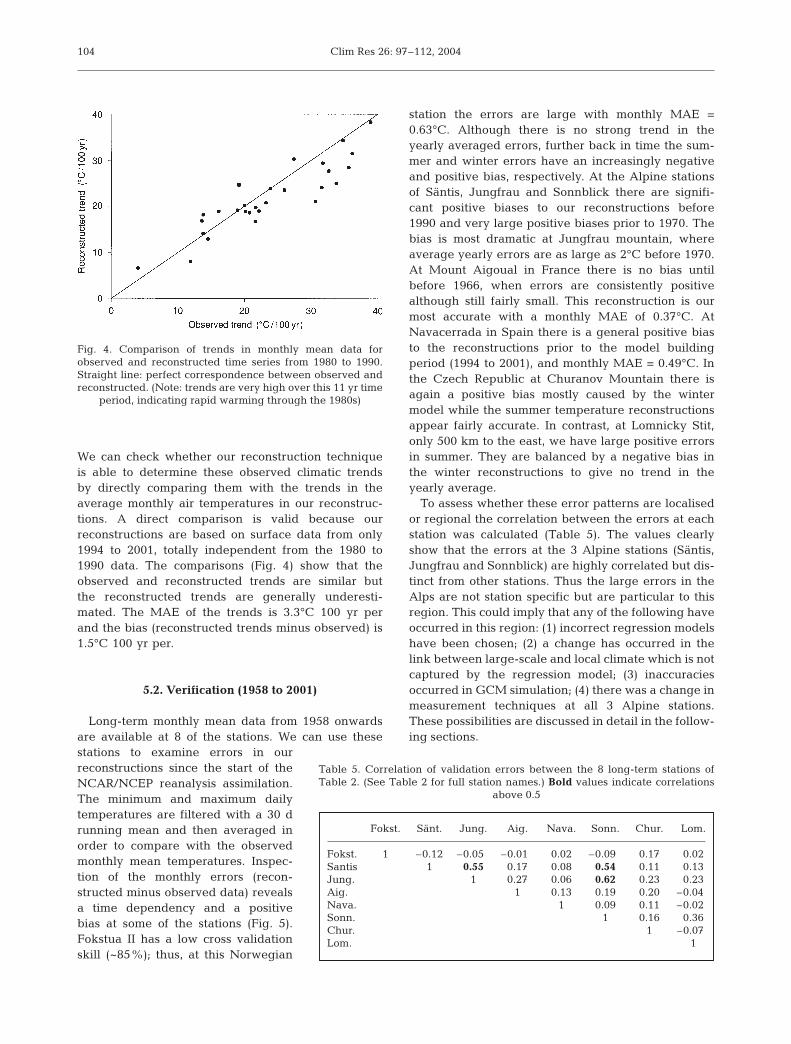
We can check whether our reconstruction techniqueis able to determine these observed climatic trendsby directly comparing them with the trends in theaverage monthly air temperatures in our reconstruc-tions. A direct comparison is valid because ourreconstructions are based on surface data from only1994 to 2001, totally independent from the 1980 to1990 data. The comparisons (Fig. 4) show that theobserved and reconstructed trends are similar butthe reconstructed trends are generally underesti-mated. The MAE of the trends is 3.3°C 100 yr perand the bias (reconstructed trends minus observed) is1.5°C 100 yr per.

5.2. Verification (1958 to 2001)

Long-term monthly mean data from 1958 onwardsare available at 8 of the stations. We can use thesestations to examine errors in ourreconstructions since the start of theNCAR/NCEP reanalysis assimilation.The minimum and maximum dailytemperatures are filtered with a 30 drunning mean and then averaged inorder to compare with the observedmonthly mean temperatures. Inspec-tion of the monthly errors (recon-structed minus observed data) revealsa time dependency and a positivebias at some of the stations (Fig. 5).Fokstua II has a low cross validationskill (~85%); thus, at this Norwegian

station the errors are large with monthly MAE =0.63°C. Although there is no strong trend in theyearly averaged errors, further back in time the sum-mer and winter errors have an increasingly negativeand positive bias, respectively. At the Alpine stationsof Säntis, Jungfrau and Sonnblick there are signifi-cant positive biases to our reconstructions before1990 and very large positive biases prior to 1970. Thebias is most dramatic at Jungfrau mountain, whereaverage yearly errors are as large as 2°C before 1970.At Mount Aigoual in France there is no bias untilbefore 1966, when errors are consistently positivealthough still fairly small. This reconstruction is ourmost accurate with a monthly MAE of 0.37°C. AtNavacerrada in Spain there is a general positive biasto the reconstructions prior to the model buildingperiod (1994 to 2001), and monthly MAE = 0.49°C. Inthe Czech Republic at Churanov Mountain there isagain a positive bias mostly caused by the wintermodel while the summer temperature reconstructionsappear fairly accurate. In contrast, at Lomnicky Stit,only 500 km to the east, we have large positive errorsin summer. They are balanced by a negative bias inthe winter reconstructions to give no trend in theyearly average.

To assess whether these error patterns are localisedor regional the correlation between the errors at eachstation was calculated (Table 5). The values clearlyshow that the errors at the 3 Alpine stations (Säntis,Jungfrau and Sonnblick) are highly correlated but dis-tinct from other stations. Thus the large errors in theAlps are not station specific but are particular to thisregion. This could imply that any of the following haveoccurred in this region: (1) incorrect regression modelshave been chosen; (2) a change has occurred in thelink between large-scale and local climate which is notcaptured by the regression model; (3) inaccuraciesoccurred in GCM simulation; (4) there was a change inmeasurement techniques at all 3 Alpine stations.These possibilities are discussed in detail in the follow-ing sections.

104

Fig. 4. Comparison of trends in monthly mean data forobserved and reconstructed time series from 1980 to 1990.Straight line: perfect correspondence between observed andreconstructed. (Note: trends are very high over this 11 yr time

period, indicating rapid warming through the 1980s)

Fokst. Sänt. Jung. Aig. Nava. Sonn. Chur. Lom.

Fokst. 1 –0.12 –0.05– –0.01– 0.02 –0.09– 0.17 0.02Santis 1 0.55 0.17 0.08 0.54 0.11 0.13Jung. 1 0.27 0.06 0.62 0.23 0.23Aig. 1 0.13 0.19 0.20 –0.04–Nava. 1 0.09 0.11 –0.02–Sonn. 1 0.16 0.36Chur. 1 –0.07–Lom. 1

Table 5. Correlation of validation errors between the 8 long-term stations ofTable 2. (See Table 2 for full station names.) Bold values indicate correlations

above 0.5

Kettle & Thompson: Statistical downscaling in European mountains 105

Fig. 5. Monthly mean validation errors (reconstructions minus observed data). (n) Summer months; (d) winter months; thick lines: yearly running mean

Clim Res 26: 97–112, 2004

5.2.1. Poor choice of downscaling model

Reconstructions at Jungfrau mountain show thelargest error trends. Therefore, to check that theseerror trends are not dependent on the form of thedownscaling model, many regression models wereexamined. Rather than choosing the single best sum-mer and winter models that gave the lowest cross vali-dation error, 400 models were examined for Jungfraumountain. These were random combinations of the 60maximum temperature models (30 for summer and 30for winter) and 60 minimum temperature modelsselected by the all-subsets regression. These modelswere then used to reconstruct mean monthly air tem-peratures since 1958 and compared with the observeddata. The errors for all 400 models followed an almostidentical pattern, showing large increases prior to1970. The range of monthly error values for eachmodel had a maximum value of 0.86°C and an averagevalue of 0.38°C. These results serve to demonstratethat the downscaling is not dependent on the exactchoice of predictors. We further note that even if theT850 and SLP predictors are erroneous the same trendin errors occurs when using just the surface minimum,maximum and mean temperatures from the nearestgrid point. In summary, the errors shown in Fig. 5 arenot simply caused by choosing a poor model.

5.2.2. Changes in the mode of circulation not capturedby our 1994 to 2001 regression models

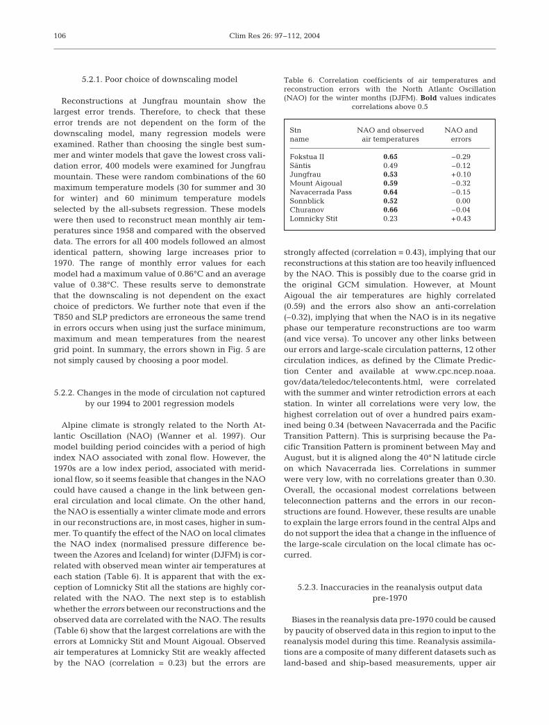
Alpine climate is strongly related to the North At-lantic Oscillation (NAO) (Wanner et al. 1997). Ourmodel building period coincides with a period of highindex NAO associated with zonal flow. However, the1970s are a low index period, associated with merid-ional flow, so it seems feasible that changes in the NAOcould have caused a change in the link between gen-eral circulation and local climate. On the other hand,the NAO is essentially a winter climate mode and errorsin our reconstructions are, in most cases, higher in sum-mer. To quantify the effect of the NAO on local climatesthe NAO index (normalised pressure difference be-tween the Azores and Iceland) for winter (DJFM) is cor-related with observed mean winter air temperatures ateach station (Table 6). It is apparent that with the ex-ception of Lomnicky Stit all the stations are highly cor-related with the NAO. The next step is to establishwhether the errors between our reconstructions and theobserved data are correlated with the NAO. The results(Table 6) show that the largest correlations are with theerrors at Lomnicky Stit and Mount Aigoual. Observedair temperatures at Lomnicky Stit are weakly affectedby the NAO (correlation = 0.23) but the errors are

strongly affected (correlation = 0.43), implying that ourreconstructions at this station are too heavily influencedby the NAO. This is possibly due to the coarse grid inthe original GCM simulation. However, at MountAigoual the air temperatures are highly correlated(0.59) and the errors also show an anti-correlation(–0.32), implying that when the NAO is in its negativephase our temperature reconstructions are too warm(and vice versa). To uncover any other links betweenour errors and large-scale circulation patterns, 12 othercirculation indices, as defined by the Climate Predic-tion Center and available at www.cpc.ncep.noaa.gov/data/teledoc/telecontents.html, were correlatedwith the summer and winter retrodiction errors at eachstation. In winter all correlations were very low, thehighest correlation out of over a hundred pairs exam-ined being 0.34 (between Navacerrada and the PacificTransition Pattern). This is surprising because the Pa-cific Transition Pattern is prominent between May andAugust, but it is aligned along the 40° N latitude circleon which Navacerrada lies. Correlations in summerwere very low, with no correlations greater than 0.30.Overall, the occasional modest correlations betweenteleconnection patterns and the errors in our recon-structions are found. However, these results are unableto explain the large errors found in the central Alps anddo not support the idea that a change in the influence ofthe large-scale circulation on the local climate has oc-curred.

5.2.3. Inaccuracies in the reanalysis output data pre-1970

Biases in the reanalysis data pre-1970 could be causedby paucity of observed data in this region to input to thereanalysis model during this time. Reanalysis assimila-tions are a composite of many different datasets such asland-based and ship-based measurements, upper air

106

Stn NAO and observed NAO andname air temperatures errors

Fokstua II 0.65 –0.29Säntis 0.49 –0.12Jungfrau 0.53 +0.10Mount Aigoual 0.59 –0.32Navacerrada Pass 0.64 –0.15Sonnblick 0.52 0.00Churanov 0.66 –0.04Lomnicky Stit 0.23 +0.43

Table 6. Correlation coefficients of air temperatures andreconstruction errors with the North Atlantc Oscillation(NAO) for the winter months (DJFM). Bold values indicates

correlations above 0.5


data, satellite observations and numerical weatherforecast output, but are obtained through the use of aconsistent circulation model. Very different weightingscan be given to these datasets. For example, surfacemeasurements over land, with strong local biases, areoften given little or no weight. Changes, through thereanalysis period, in the distribution, types and quality ofthe observations such as those of radiosonde and satellitecan potentially lead to substantial inhomogeneities (Up-pala 1997). Trenberth et al. (2001) give an example forthe tropics with jumps to warmer values below 500 mb in1986 and 1989. Other analyses point to jumps aroundNovember 1978 between the pre- and post-satelliteperiods at the 100 mb level. Shifts in the reanalysismoisture fields (Trenberth & Guillemot 1998, Poccard etal. 2000) have similarly been noted in the mid-1970s andmid-1980s. Problems have also been recorded forsurface pressure fields in the North Atlantic before 1968,where all observed pressure data below 1000 mb occur-ring during extra tropical cyclones were not input to thereanalysis model due to an error (Bob Kistler, http://wwwt.emc.ncep.noaa.gov/gmb/bkistler/psfc/psfc.html).However, it is unlikely that these discrete events couldcause the general error trend we observe for the Alpinestations.

5.2.4. Changes in measurement technique or changesto the type and location of the stations

Another cause of the large errors we find prior to1970 could be changes in measurement technique orchanges to the type and location of the mountain sta-tions. According to Weber (1993), between 1978 and1981 some of the Swiss stations were completelychanged to automatic measurement systems with elec-tronic thermometers and a nearly continuous record-ing of data every 10 min. In 1961 the station at Säntischanged from a small metallic shelter attached to thenorth wall of a building to a standard Stevenson screen(Weber 1993). The time of reading was also changed inSwitzerland around 1970 (Weber 1993) with the bigdifference that the reading of the maximum tempera-ture was changed from evening to morning. Asdescribed by Karl et al. (1986), this can have a largeeffect on daily minimum and maximum values. Thus, itis possible that a bias in the daily mean temperature(the arithmetic mean of the maximum and minimum)occurs around 1970 at the Swiss stations, which coin-cides with the errors found in our reconstructions. Toinvestigate this source of error further we made 3 typesof check. Firstly, we used Alexandersson’s (1986)method to recheck the homogeneity of the long-termmountain station data. Secondly, we compared thetrends in our reconstruction with those described by

Weber et al. (1997) and Beniston et al. (1994) for theAlps. Thirdly we compared our reconstructions withthe observed monthly data from the gridded homo-genised dataset, CRUTEM1 (Jones 1994).

Alexandersson’s (1986) method reveals no majorhomogeneities, discrepancies, or sharp breaks in therecords of the 3 Alpine stations of Jungfrau, Säntis orSonnblick, when they are taken in comparison to oneanother and to a lowland reference series based onBasel, Geneva, Milan and Vienna. However, we notethat the trends in mean temperature at Jungfrau (1958to 1990) are the most extreme (most positive) of all 7 ofthese series, by a factor of almost 2. We find many sim-ilarities between our reconstructions and the trendsreported by Weber et al. (1997) and Beniston et al.(1994). For example in the Alps the strongest warmingtrends in our reconstructions (Table 7) are for thewinter season, especially in maximum temperatures.Weber et al. (1997, their Table IV) and Beniston et al.(1994, their Figs. 18 & 19) find exactly the same. Fur-thermore, Weber et al. (1997, their Table IV) reportthat the strongest cooling trends in the Alpine areatook place in the eastern Alps, particularly in summer(JJA) and autumn (SON) months at mountain sites. Wesimilarly reconstruct the most negative trends in theautumn at our mountain sites in the NE Alps (Table 7).Thus, even in the 1 region (Alps), and 1 time period(pre-1970), where the bias in our reconstructions issomewhat higher than might have been hoped for (seeSäntis, Jungfrau and Sonnblick in Fig. 5), we never-theless correctly deduce the main features not only ofthe inter-annual variability but also of the long-termtrends. One difference between our mountain sitereconstructions and the trends reported by other work-ers is for autumn temperatures in the central Alps. Wededuce (Table 7) an average cooling trend of –1.33°Cper 100 yr; however, in contrast Weber et al. (1997),Beniston et al. (1994) and CRUTEM1 all report awarming. Turning our attention more closely to theCRUTEM1 gridded homogenised dataset, the gridsquare which contains Jungfrau mountain does notcontain any data but the adjacent square (45–50° N ×10–15° E) contains nearly continuous monthly dataover 1958 to 2001. The correlation between the gridsquare CRUTEM1 temperatures and our reconstructedtemperatures at Jungfrau mountain is 0.65 (annualcycles removed), indicating that this comparison isvalid. The difference between our reconstructions atJungfrau mountain and the mean temperature in thegrid square is shown in Fig. 6. The difference betweenthese 2 time series remains approximately constantover the whole time period. The same result was foundfor both Sonnblick and Säntis. We note in Table 8 thatthe main negative temperature trends in CRUTEM1(1958 to 2001) are for the autumn, in east Europe and

107

Clim Res 26: 97–112, 2004

NE Alps. Otherwise, CRUTEM1 trends are positive, ornegligible. Our one discrepancy with CRUTEM1 (1958to 2001), and with Weber et al. (1997) and Beniston etal. (1994), is for the central Alps in autumn, where weincorrectly reconstruct a cooling that mainly occurredfurther to the east.

In summary, verification of our downscaling modelsis generally very good. However, high bias is foundpre-1970, especially at Jungfrau mountain and to alesser extent Sonnblick and Säntis. These discrepan-cies can be mainly explained by difficulties with theearly observations at Jungfrau, and to a certain extent

by problems with our pre-1970 autumn downscaling inthe central Alps.

6. LONG-TERM TRENDS ACROSS EUROPE

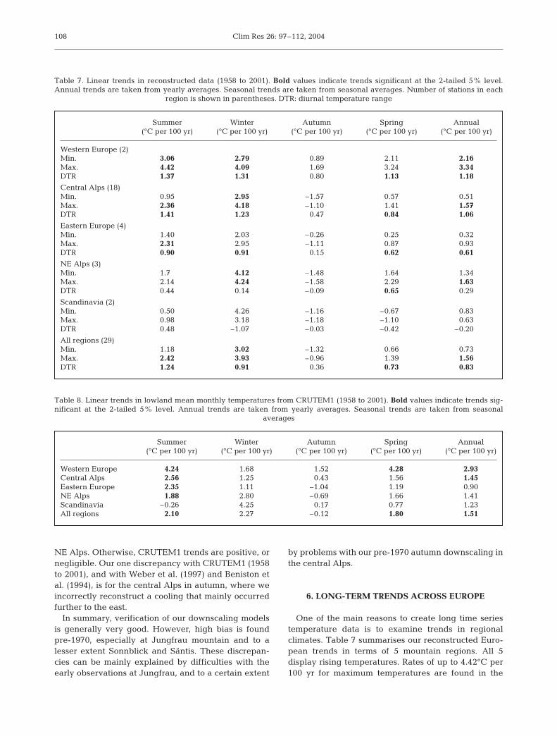
One of the main reasons to create long time seriestemperature data is to examine trends in regionalclimates. Table 7 summarises our reconstructed Euro-pean trends in terms of 5 mountain regions. All 5display rising temperatures. Rates of up to 4.42°C per100 yr for maximum temperatures are found in the

108

Summer Winter Autumn Spring Annual (°C per 100 yr) (°C per 100 yr) (°C per 100 yr) (°C per 100 yr) (°C per 100 yr)

Western Europe (2)Min. 3.06 2.79 0.89 2.11 2.16Max. 4.42 4.09 1.69 3.24 3.34DTR 1.37 1.31 0.80 1.13 1.18

Central Alps (18) Min. 0.95 2.95 –1.57– 0.57 0.51Max. 2.36 4.18 –1.10– 1.41 1.57DTR 1.41 1.23 0.47 0.84 1.06

Eastern Europe (4)Min. 1.40 2.03 –0.26– 0.25 0.32Max. 2.31 2.95 –1.11– 0.87 0.93DTR 0.90 0.91 0.15 0.62 0.61

NE Alps (3)Min. 1.70 4.12 –1.48– 1.64 1.34Max. 2.14 4.24 –1.58– 2.29 1.63DTR 0.44 0.14 –0.09– 0.65 0.29

Scandinavia (2)Min. 0.50 4.26 –1.16– –0.67– 0.83Max. 0.98 3.18 –1.18– –1.10– 0.63DTR 0.48 –1.07– –0.03– –0.42– –0.20–

All regions (29)Min. 1.18 3.02 –1.32– 0.66 0.73Max. 2.42 3.93 –0.96– 1.39 1.56DTR 1.24 0.91 0.36 0.73 0.83

Table 7. Linear trends in reconstructed data (1958 to 2001). Bold values indicate trends significant at the 2-tailed 5% level.Annual trends are taken from yearly averages. Seasonal trends are taken from seasonal averages. Number of stations in each

region is shown in parentheses. DTR: diurnal temperature range

Summer Winter Autumn Spring Annual (°C per 100 yr) (°C per 100 yr) (°C per 100 yr) (°C per 100 yr) (°C per 100 yr)

Western Europe 4.24 1.68 1.52 4.28 2.93Central Alps 2.56 1.25 0.43 1.56 1.45Eastern Europe 2.35 1.11 –1.04– 1.19 0.90NE Alps 1.88 2.80 –0.69– 1.66 1.41Scandinavia –0.26– 4.25 0.17 0.77 1.23All regions 2.10 2.27 –0.12– 1.80 1.51

Table 8. Linear trends in lowland mean monthly temperatures from CRUTEM1 (1958 to 2001). Bold values indicate trends sig-nificant at the 2-tailed 5% level. Annual trends are taken from yearly averages. Seasonal trends are taken from seasonal

averages


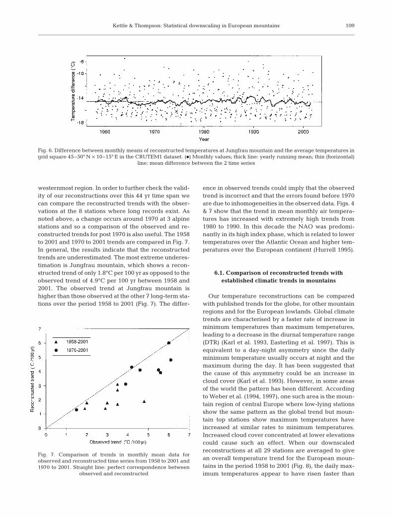
westernmost region. In order to further check the valid-ity of our reconstructions over this 44 yr time span wecan compare the reconstructed trends with the obser-vations at the 8 stations where long records exist. Asnoted above, a change occurs around 1970 at 3 alpinestations and so a comparison of the observed and re-constructed trends for post 1970 is also useful. The 1958to 2001 and 1970 to 2001 trends are compared in Fig. 7.In general, the results indicate that the reconstructedtrends are underestimated. The most extreme underes-timation is Jungfrau mountain, which shows a recon-structed trend of only 1.8°C per 100 yr as opposed to theobserved trend of 4.9°C per 100 yr between 1958 and2001. The observed trend at Jungfrau mountain ishigher than those observed at the other 7 long-term sta-tions over the period 1958 to 2001 (Fig. 7). The differ-

ence in observed trends could imply that the observedtrend is incorrect and that the errors found before 1970are due to inhomogeneities in the observed data. Figs. 4& 7 show that the trend in mean monthly air tempera-tures has increased with extremely high trends from1980 to 1990. In this decade the NAO was predomi-nantly in its high index phase, which is related to lowertemperatures over the Atlantic Ocean and higher tem-peratures over the European continent (Hurrell 1995).

6.1. Comparison of reconstructed trends withestablished climatic trends in mountains

Our temperature reconstructions can be comparedwith published trends for the globe, for other mountainregions and for the European lowlands. Global climatetrends are characterised by a faster rate of increase inminimum temperatures than maximum temperatures,leading to a decrease in the diurnal temperature range(DTR) (Karl et al. 1993, Easterling et al. 1997). This isequivalent to a day-night asymmetry since the dailyminimum temperature usually occurs at night and themaximum during the day. It has been suggested thatthe cause of this asymmetry could be an increase incloud cover (Karl et al. 1993). However, in some areasof the world the pattern has been different. Accordingto Weber et al. (1994, 1997), one such area is the moun-tain region of central Europe where low-lying stationsshow the same pattern as the global trend but moun-tain top stations show maximum temperatures haveincreased at similar rates to minimum temperatures.Increased cloud cover concentrated at lower elevationscould cause such an effect. When our downscaledreconstructions at all 29 stations are averaged to givean overall temperature trend for the European moun-tains in the period 1958 to 2001 (Fig. 8), the daily max-imum temperatures appear to have risen faster than

109

Fig. 6. Difference between monthly means of reconstructed temperatures at Jungfrau mountain and the average temperatures ingrid square 45–50° N × 10–15° E in the CRUTEM1 dataset. (d) Monthly values; thick line: yearly running mean; thin (horizontal)

line: mean difference between the 2 time series

Fig. 7. Comparison of trends in monthly mean data forobserved and reconstructed time series from 1958 to 2001 and1970 to 2001. Straight line: perfect correspondence between

observed and reconstructed

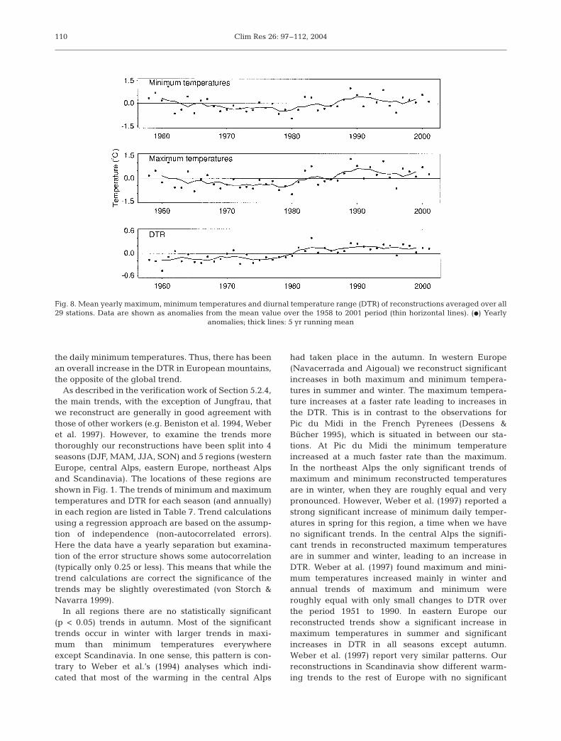
Clim Res 26: 97–112, 2004

the daily minimum temperatures. Thus, there has beenan overall increase in the DTR in European mountains,the opposite of the global trend.

As described in the verification work of Section 5.2.4,the main trends, with the exception of Jungfrau, thatwe reconstruct are generally in good agreement withthose of other workers (e.g. Beniston et al. 1994, Weberet al. 1997). However, to examine the trends morethoroughly our reconstructions have been split into 4seasons (DJF, MAM, JJA, SON) and 5 regions (westernEurope, central Alps, eastern Europe, northeast Alpsand Scandinavia). The locations of these regions areshown in Fig. 1. The trends of minimum and maximumtemperatures and DTR for each season (and annually)in each region are listed in Table 7. Trend calculationsusing a regression approach are based on the assump-tion of independence (non-autocorrelated errors).Here the data have a yearly separation but examina-tion of the error structure shows some autocorrelation(typically only 0.25 or less). This means that while thetrend calculations are correct the significance of thetrends may be slightly overestimated (von Storch &Navarra 1999).

In all regions there are no statistically significant(p < 0.05) trends in autumn. Most of the significanttrends occur in winter with larger trends in maxi-mum than minimum temperatures everywhereexcept Scandinavia. In one sense, this pattern is con-trary to Weber et al.’s (1994) analyses which indi-cated that most of the warming in the central Alps

had taken place in the autumn. In western Europe(Navacerrada and Aigoual) we reconstruct significantincreases in both maximum and minimum tempera-tures in summer and winter. The maximum tempera-ture increases at a faster rate leading to increases inthe DTR. This is in contrast to the observations forPic du Midi in the French Pyrenees (Dessens &Bücher 1995), which is situated in between our sta-tions. At Pic du Midi the minimum temperatureincreased at a much faster rate than the maximum.In the northeast Alps the only significant trends ofmaximum and minimum reconstructed temperaturesare in winter, when they are roughly equal and verypronounced. However, Weber et al. (1997) reported astrong significant increase of minimum daily temper-atures in spring for this region, a time when we haveno significant trends. In the central Alps the signifi-cant trends in reconstructed maximum temperaturesare in summer and winter, leading to an increase inDTR. Weber at al. (1997) found maximum and mini-mum temperatures increased mainly in winter andannual trends of maximum and minimum wereroughly equal with only small changes to DTR overthe period 1951 to 1990. In eastern Europe ourreconstructed trends show a significant increase inmaximum temperatures in summer and significantincreases in DTR in all seasons except autumn.Weber et al. (1997) report very similar patterns. Ourreconstructions in Scandinavia show different warm-ing trends to the rest of Europe with no significant

110

Fig. 8. Mean yearly maximum, minimum temperatures and diurnal temperature range (DTR) of reconstructions averaged over all29 stations. Data are shown as anomalies from the mean value over the 1958 to 2001 period (thin horizontal lines). (d) Yearly

anomalies; thick lines: 5 yr running mean


seasonal trends, agreeing with Diaz & Bradley(1997), who found Scandinavia does not show therecent warming seen elsewhere.

Overall, our results for high elevation sites suggestthat the strongest warming has occurred in westernEurope with rather weaker warming in eastern Europeand Scandinavia. All regions except Scandinavia showa faster increase in maximum temperature than in min-imum temperature, occurring mainly in winter. Fur-thermore our reconstructions indicate that on averagethe DTR has increased. These results, although contra-dicting some of Weber et al.’s (1994, 1997) analysis dis-play the general spatial pattern observed by Diaz &Bradley (1997) regarding large warming trends inwestern Europe and small warming trends in easternEurope and Scandinavia.

6.2. Comparison with lowland trends

It is also possible to compare our reconstructedtrends with trends in mean temperatures determinedfrom predominantly lowland data. To do this we aver-aged mean monthly data from the relevant gridsquares in the CRUTEM1 (Jones 1994) dataset. Thecomparisons (Table 8) show the CRUTEM1 trendshave much in common with our reanalysis downscal-ing. Indeed, the broad spatio-temporal patterns oftemperature trends across Europe are very compara-ble. Here we focus on the similarities. First, theannual trends are highest for western Europe, andlowest for eastern Europe and Scandinavia. Secondly,the seasonal trends also show many common fea-tures. Trends are strong for the summer months par-ticularly in western Europe, but with both our recon-structed mountain trends and the ‘lowland’ trendsshowing little or no trend in Scandinavia. In winter,trends have in general been lower. Once again Scan-dinavia is the exception with both our upland recon-structions and the ‘lowland’ trends being higher thanelsewhere in Europe. Autumn trends are low every-where in both datasets. Finally, in spring, westernEurope and to a lesser extent NE Europe have expe-rienced the high trends. However, while the spatio-temporal patterns match well, the magnitudes of thetrends tend to be lower in our reconstructions formountain regions. We have an average annual tem-perature increase, over all regions, of only 1.1°C per100 yr in comparison to 1.5°C per 100 yr in the ‘low-lands’. In general, the magnitudes of the trends inmaximum temperature in the mountains are compa-rable with magnitudes of the trends in mean temper-ature in the lowlands. Once again Scandinaviabreaks the general rule set by the normal Europeansituation.

7. CONCLUSIONS

In this work linear regression models built on short-term daily data (1994 to 2001) are used to reconstructdaily mean, minimum and maximum air temperaturesback to 1958 at 29 mountain weather stations. Thisstudy attempts to analyse the accuracy of these down-scaled air temperatures by answering the 8 questionsraised in the ‘Introduction’. Below is a summary of theanswers:

(1) Is there a difference in the accuracy of down-scaled minimum, maximum and mean daily air tem-peratures? Yes, mean air temperatures are the mostaccurately downscaled. Minimum daily temperaturesare the least accurate.

(2) Is there a seasonal difference in downscalingaccuracy? Yes. The skill is higher in winter. However,the natural variability is larger in winter so theabsolute errors are generally higher than in summer.

(3) Are temporal and spatial structures in the tem-perature series correctly downscaled? No, the persis-tence (lag-1 correlations) is consistently overestimated,particularly for the daily minimum and maximum airtemperature reconstructions. The spatial correlationsare also overestimated.

(4) Which reanalysis variables are the most impor-tant predictors? The air temperature at the 850 mbpressure level at the reanalysis grid point nearest tothe station of interest is the most used variable. Princi-pal components of SLP and T850 are more often usedin the winter rather than summer models. In generalthe summer models require about half the number ofpredictors used by the winter models.

(5) Can we accurately reconstruct air temperaturesbetween 1980 and 1990? Over this period there is verylittle bias (0.09°C) in the winter reconstructions butsummer temperatures are slightly over estimated(0.22°C). Individual monthly mean temperatures canbe reproduced to within ~0.5°C, and there are notrends in the errors.

(6) Can we accurately reconstruct air temperaturesback to 1958? In some locations the reconstructions backto 1958 are reasonable, but at 3 alpine stations the ap-parent errors increase prior to 1970. Whether this changeis due to inaccurate downscaling, inaccuracies in the re-analysis assimilation or inhomogeneities in the observedclimate data remains to be determined. Our validationand verification studies point to caution in extrapolatingthese models further back in time than 1970.

(7) How accurate are the long-term climatic trendsderived from reconstructed temperatures? In generalthe long-term trends are underestimated in the recon-structed data. This underestimation is very pro-nounced for the time periods 1958 to 2001 and 1970 to2001, and occurs to a lesser extent in 1980 to 1990.

111

Clim Res 26: 97–112, 2004

(8) How do the reconstructed trends compare withestablished climate trends? Overall, the reconstruc-tions indicated that maximum temperatures are risingfaster than minimum temperatures, resulting in anincrease in the DTR from 1958 to 2001. This is in dis-agreement with some published trends (e.g. Weber1994, 1997) which show maximum and minimum tem-peratures to be increasing at approximately equalrates in the European mountains with insignificantchanges in DTR. However, our reconstructed trends formaximum temperatures are very similar to those formean lowland temperatures.

Acknowledgements. Funding was provided by the EuropeanUnion Framework V project EMERGE (European Mountainlake Ecosystems: Regionalisation, diaGnostics & socio-eco-nomic Evaluation; contract no. EVK1-CT-1999-00032). Pro-cessed homogeneous gridded climate data are from the Cli-matic Research Unit (CRU) with source data from theNCEP/NCAR Reanalysis Project. The observed surface dataare from World Meteorological Organisation (WMO) observa-tories obtained from the National Climatic Data Center(NCDC). The Jones CRUTEM1 gridded data are from CRU.None of our work would have been possible without thesevaluable climate resources.

LITERATURE CITED

Alexandersson H (1986) A homogeneity test applied to pre-cipitation data. J Clim 6:661–675

Beniston M, Rebetez M, Giorgi F, Marinucci MR (1994) Ananalysis of regional climate change in Switzerland. TheorAppl Clim 49:135–159

Beniston M, Diaz HF, Bradley RS (1997) Climatic change athigh elevation sites: an overview. Clim Change 36:233–251

Dessens J, Bücher A (1995) Changes in minimum and maxi-mum temperatures at the Pic du Midi in relation withhumidity and cloudiness. Atmos Res 37:147–162

Diaz HF, Bradley RS (1997) Temperature variations during thelast century at high elevation sites. Clim Change 36:253–279

Easterling DR, Horton B, Jones PD, Peterson TC and 7 others(1997) Maximum and minimum temperature trends for theglobe. Science 277:364–367

Grotch S, MacCracken M (1991) The use of general circula-tion models to predict regional climate change. J Clim 4:284–303

Hurrell JW (1995) Decadal trends in North Atlantic Oscilla-tion: regional temperatures and precipitation. Science269:676–679

Huth R (1997) Potential of continental-scale circulation for thedetermination of local daily surface variables. Theor ApplClim 56:165–186

Huth R (1999) Statistical downscaling in central Europe: eval-

uation of methods and potential predictors. Clim Res 13:91–101

Huth R (2002) Statistical downscaling of daily temperature incentral Europe. J Clim 15:1731–1742

IPCC (Intergovernmental Panel on Climate Change) (2001)Climate change 2001: the scientific basis. CambridgeUniversity Press, Cambridge

Jones PD (1994) Hemispheric surface air temperature varia-tions: a reanalysis and an update to 1993. J Clim 7:1794–1802

Kalnay E, Kanamitsu M, Kistler R, Collins W and 17 others(1996) The NCEP/NCAR 40-year Reanalysis Project. BullAm Meteorol Soc 77:437–471

Karl TR, Williams CN, Young PJ (1986) A model to estimatethe time of observation bias associated with monthly meanmaximum, minimum and mean temperatures for theUnited States. J Clim Appl Meteorol 25:145–160

Karl TR, Jones PD, Knight RW, Kukla G and 6 others (1993)Asymmetric trends of daily maximum and minimumtemerature. Bull Am Meteorol Soc 74:1007–1023

Lorenz EN (1956) Empirical orthogonal functions and statisti-cal weather prediction. Statistical Forecasting ScientificRep. 1. Department of Meteorology, Massachusetts Insti-tute of Technology, Cambridge, MA

Poccard I, Janicot S, Camberlin P (2000) Comparison of rain-fall structures between NCEP/NCAR reanalyses andobserved data over tropical Africa. Clim Dyn 16:897–915

Trenberth KE, Guillemot (1998) Evaluation of the atmosphericmoisture and hydrological cycle in the NCEP/NCARreanalyses. Clim Dyn 14:213–231

Trenberth KE, Stepaniak DP, Hurrell JW, Fiorino M (2001)Quality of reanalyses in the Tropics. J Clim 14:1499–1510

Uppala S (1997) Observing system performance in ERA.ECMWF Reanalysis Project Rep. 3. The National Acade-mic Press, Reading

von Storch H, Navarra A (1999) Analysis of climate variability,2nd edn. Springer-Verlag, Berlin

Wanner H, Rickli R, Salvisberg E, Schmutz C, Schuepp M(1997) Global climate change and variability and its in-fluence on alpine climate—concepts and observations.Theor Appl Clim 58:221–243

Weber RO (1993) Influence of different daily mean formulason monthly and annual averages of temperature. TheorAppl Clim 47:205–213

Weber RO, Talkner P, Stefanicki G (1994) Asymmetric diurnaltemperature change in the Alpine region. Geophys ResLett 21:673–676

Weber RO, Talkner P, Auer I, Bohm R, Gajic-capka M, Zani-novic K, Brazdil R, Fasko P (1997) 20th-century changes oftemperature in the mountain regions of central Europe.Clim Change 36:327–344

Wigley TML, Jones PD, Briffa KR, Smith G (1990) Obtainingsub-grid-scale information from coarse-resolution generalcirculation model output. J Geophys Res 95:1943–1953

Wilby RL, Wigley TML (1997) Downscaling general circula-tion model output: a review of methods and limitations.Prog Phys Geogr 21:530–548

Zorita E, von Storch H (1999) The analog method as a simplestatistical downscaling technique: comparison with morecomplicated methods. J Clim 12:2474–2489

112

Editorial responsibility: Clare Goodess,Norwich, UK

Submitted: February 17, 2003; Accepted: March 10, 2004Proofs received from author(s): April 26, 2004

Documents

Statistical downscaling in European mountains