Statistical Inference for Topological Data Analysis

PhD Thesis Proposal

Fabrizio LecciDepartment of Statistics

Carnegie Mellon University

Thesis Committe

Jessi CisewskiFrederic Chazal

Alessandro RinaldoRyan Tibshirani

Larry Wasserman

January 31, 2014

Abstract

Topological Data Analysis (TDA) is an emerging area of research at the intersection ofalgebraic topology and computational geometry, aimed at describing, summarizing andanalyzing possibly high-dimensional data using low-dimensional algebraic representa-tions. Recent advances in computational topology have made it possible to actuallycompute topological invariants from data. These novel types of data summaries havebeen used successfully in a variety of applied problems, and their potential for high-dimensional statistical inference appears to be significant. Nonetheless, the statisticalproperties of the data summaries produced in TDA and, more generally, of the usuallyheuristic data-analytic methods they are part of, have remained largely unexplored bystatisticians. Our analysis involves the tools of persistent homology, the main methodof TDA for measuring the topological features of shapes and functions at different res-olutions. A major part of our research also focuses on cluster trees and Reeb graphs,which provide a simple yet meaningful abstraction of the input domain of a functionby means of the topological changes in its level sets.The main goal of this thesis is to contribute to the development of a statistical theoryfor TDA and to further propose new and statistically principled methodologies to im-prove and extend the applicability of the algorithms of TDA. In particular, we will (1)study tests of significance and confidence intervals to separate topological signal fromtopological noise; (2) explore new methods for topological dimensional reduction; (3)determine how our methods contribute to reduce computational costs, which currentlyrepresent an obstacle in TDA.

2

Contents

1 Introduction 4

2 Persistent Homology 5

2.1 Background . . . . . . . . . . . . . . . . . . . . . . . . . . . . . . . . . . . . 5

2.1.1 Persistent Homology of the distance function . . . . . . . . . . . . . . 6

2.1.2 Persistent Homology of the density function. . . . . . . . . . . . . . . 7

2.1.3 Persistence Diagrams and Stability . . . . . . . . . . . . . . . . . . . 8

2.1.4 Persistence Landscapes . . . . . . . . . . . . . . . . . . . . . . . . . . 9

2.2 Research Plan . . . . . . . . . . . . . . . . . . . . . . . . . . . . . . . . . . . 10

2.2.1 Preliminary Work . . . . . . . . . . . . . . . . . . . . . . . . . . . . . 11

2.2.2 Research Aim . . . . . . . . . . . . . . . . . . . . . . . . . . . . . . . 13

3 Density Clustering 15

3.1 Background . . . . . . . . . . . . . . . . . . . . . . . . . . . . . . . . . . . . 15

3.1.1 Level Set Trees . . . . . . . . . . . . . . . . . . . . . . . . . . . . . . 15

3.2 Research Plan . . . . . . . . . . . . . . . . . . . . . . . . . . . . . . . . . . . 16

3

1 IntroductionTopological Data Analysis (TDA) refers to a collection of methods for finding topologicalstructure in data (Carlsson, 2009). Recent advances in computational topology have made itpossible to actually compute topological invariants from data. The input of these procedurestypically takes the form of a point cloud, regarded as possibly noisy observations from anunknown lower-dimensional set S whose interesting topological features were lost duringsampling. The output is a collection of data summaries that are used to estimate thetopological features of S.

These novel types of data summaries have been used successfully in a variety of applied prob-lems, ranging from medical imaging and neuroscience (Chung et al., 2009; Pachauri et al.,2011) to cosmology (Sousbie, 2011; van de Weygaert et al., 2011; Cisewski et al., 2014),sensor networks (de Silva and Ghrist, 2007) landmark-based shape data analyses (Gambleand Heo, 2010), and cellular biology (Kasson et al., 2007). Nonetheless, the statistical prop-erties of the data summaries produced in TDA and, more generally, of the usually heuristicdata-analytic methods they are part of, have remained largely unexplored by statisticians.

One approach to TDA is persistent homology (Edelsbrunner and Harer, 2010), a methodfor studying the homology at multiple scales simultaneously. More precisely, it provides aframework and efficient algorithms to quantify the evolution of the topology of a family ofnested topological spaces. Given a real-valued function f , persistent homology describeshow the topology of the lower level sets {x : f(x) ≤ t} (or upper level sets {x : f(x) ≥ t})change as t increases from −∞ to ∞ (or decreases from ∞ to −∞). This information isencoded in the persistence diagram, a multiset of points in the plane, each correspondingto the birth and death of a homological feature that existed for some interval of t. Thanksto their stability properties (Cohen-Steiner et al., 2007; Chazal et al., 2012), persistencediagrams provide relevant multi-scale topological information about the data. One of thekey challenges is persistent homology is to find a way to isolate the points of the persistencediagram representing the topological noise. In Fasy et al. (2013) and Chazal et al. (2013b)we propose several statistical methods to construct confidence sets for persistence diagramsand other summary functions that allow us to separate topological signal from topologicalnoise. The research objective of this proposal is to develop new theories and methods toimprove and extend the applicability of the algorithms of persistent homology.

A second sect of research activities pertains to the related task of clustering in high dimen-sions. Density clustering allows us to identify and visualize the spatial organization of thedata, without specific knowledge about the data generating mechanism and in particularwithout any a priori information about the number of clusters. We will consider the sublevelset tree as a topological descriptor and study its properties, including the notion of distancebetween trees that will lead to the definition of inferential procedures. We will also try toextend the results to a related descriptor, the Reeb graph, which encodes information on thelevel sets of a function and on the topology of the input domain (Biasotti et al., 2008).

4

2 Persistent HomologyWe provide an informal description of the methods of homology and persistent homology.For rigorous expositions, the reader is referred to the textbooks Munkres (1984); Zomorodian(2005); Edelsbrunner and Harer (2010) and the introductory reviews Edelsbrunner and Harer(2008); Chazal et al. (2012).

2.1 Background

Homology is a mathematical formalism used to summarize the overall connectivity of atopological space. The homology of a space S is a collection of abelian groups of differentdimensions, the pth dimensional group encoding the pth dimensional “holes” in S. The pthhomology group Hp(S) is the set of equivalence classes of loops enclosing the pth dimensionalholes, and its rank βp is called the pth Betti number. Roughly speaking, the pth Betti numberβp is the number of pth dimensional holes in S, so that β0 is the number of connectedcomponents of S, β1 is the number of loops, β2 is the number of enclosed voids and so on.See Figure 1.

Figure 1: The circle has one connected component and one 1-dimensional hole: β0 =1, β1 = 1. A sphere in R3 has one connected component and one 2-dimensional hole (void):β0 = 1, β1 = 0, β2 = 1. The torus has one connected component, two 1-dimensional holes(the two non equivalent circles in red) and one enclosed void: β0 = 1, β1 = 2, β2 = 1.

Persistent Homology is the main tool of TDA for measuring the scale or resolution of topo-logical features. Given a function f : X → R, defined for a triangulable subspace of RD,persistent homology describes the changes in the topology of the lower (or upper) level setsof f . For example, consider the lower level sets Lt = {x ∈ X : f(x) ≤ t}. The index t can beseen as a scale parameter leading to a filtration of subspaces, such that Lt ⊆ Ls for all t ≤ s.Such a filtration induces a family {H(Lt) : t ∈ R} of homology groups and the inclusionsLt ↪→ Ls induce a family of homomorphisms H(Lt)→ H(Ls). Persistent homology describesf with the persistence diagram, a multiset of points in the plane, each corresponding to thebirth and death of a homological feature that existed for some interval of t. The point (s, t)in the diagram represents a distinct topological feature that existed in H(Lr) for r ∈ [s, t).

In the following we focus on the persistent homology of distance functions and densityfunctions, providing more details on the construction of the persistence diagrams and a fewclarifying examples.

5

2.1.1 Persistent Homology of the distance function

First, we consider the case where f is the distance function. Let S be a compact subset ofRD and let dS : RD → R be the distance function to S:

dS(x) = infy∈S‖y − x‖2.

Consider the sub-level set Lt = {x : dS(x) ≤ t}; note that S = L0. As t varies from 0 to∞, the set Lt changes. Persistent homology summarizes how the topological features of Ltchange as a function of t. Key topological features of a set include the connected components(the zeroth order homology), the tunnels (the first order homology), voids (second orderhomology), etc. These features can appear (be born) and disappear (die) as t increases. Forexample, connected components of Lt die when they merge with other connected components.Each topological feature has a birth time b and a death time d. In general, there will be aset of features with birth and death times (b1, d1), . . . , (bm, dm). These points can be plottedon the plane, resulting in a persistence diagram P . We view the persistence diagram as atopological summary of the input function or data.

����������

��

Figure 2: Left: 30 data points S30 sampled from the circle of radius 2. Middle left:sub-levels set L0.5 = {x : dS30 ≤ 0.5}; for t = 0.5 the sub-level set consists of two connectedcomponents and zero loops. Middle right: sub-levels set L0.8 = {x : dS30 ≤ 0.8}; aswe keep increasing t we assist at the birth and death of topological features; at t = 0.8one of the connected components dies (is merged with the other one) and a 1-dimensionalhole is formed; this loop will die at t = 2, when the pink balls representing the distancefunction will touch each other in the center of the circle. Right: the empirical persistencediagram summarizes the topological features of the sampled points. The black dots repre-sent the connected components: 30 connected components are present at t = 0 and theyprogressively die as t increases, leaving only one connected component that persists forlarge values of t. The red triangle represent the unique 1-dimensional hole that is formedat t = 0.8 and dies at t = 2.

Given data points Sn = {X1, . . . , Xn}, we are interested in understanding the homology ofthe d-dimensional compact topological space S ⊂ RD from which the data were sampled. Ifour sample is dense enough then Lt = {x : dSn(x) ≤ t} has the same homology of S for aninterval of values of t. Choosing the right t is a difficult task: small t will have the homology

6

of n points and large t will have the homology of a single point. Using persistent homology,we avoid choosing a single t by assigning a persistence value to each non-trivial topologicalfeature that is realized for some non-negative t. As t varies, we summarize birth and deathof topological features of Sn using the empirical persistence diagram P . We treat P as anestimate of the unobserved persistence diagram P of the underlying space S. Points nearthe diagonal in the persistence diagram have short lifetimes and are considered “topologicalnoise”. In most applications we are interested in features that we can distinguish from noise;that is, those features that persist for a large range of values of t. Figure 2 shows an examplethat clarifies the concepts described above.

Despite the seemingly geometric nature of homology invariants, they are in fact purely com-binatorial quantities, which are computed by triangulating a topological space with simplicialcomplexes (Zomorodian and Carlsson, 2005). In some practical applications, the number ofsimplices can be so large that the exact computation of the persistent homology becomesprohibitive. Efficient approaches for approximating the persistent homology will be usefulonly if combined with statistical guarantees.

2.1.2 Persistent Homology of the density function.

Most of the literature on computational topology focuses on the distance function. Alter-natively, one can use the data to construct a smooth density estimator and then find thepersistence diagram defined by a filtration of the upper level sets of the density estimator.This strategy is discussed in detail in Fasy et al. (2013), where it is shown that the density-based method is very insensitive to outliers. A different approach to smoothing based ondiffusion distances is discussed in Bendich et al. (2011).

Figure 3: Left: 500 data points sampled from the circle of radius 1. Middle left: Gaus-sian kernel density estimator with bandwidth h = 0.3. Middle right: upper-levels setU0.1 = {x : ph ≤ 0.1}. Right: the empirical density persistence diagram summarizes thetopological features of upper level sets of the kernel density estimator. The black dotsrepresent the connected components: 2 connected components appear around t = 0.27,but one of them immediately dies (is merged to the other one). The red triangle representthe unique 1-dimensional hole that is formed at t = 0.12 and dies at t = 0.01.

7

Let X1, . . . , Xni.i.d.∼ P , where Xi ∈ RD. We assume that the support of P is d-dimensional

compact manifold M. Define

ph(x) =

∫M

1

hDK

(||x− u||

h

)dP (u). (1)

Then ph is the density of the probability measure Ph which is the convolution Ph = P ?Kh

where Kh(A) = h−DK(h−1A) and K(A) =∫AK(t)dt. That is, Ph is a smoothed version of

P . The standard estimator for ph is the kernel density estimator

ph(x) =1

n

n∑i=1

1

hDK

(||x−Xi||

h

). (2)

It is easy to see that E(ph(x)) = ph(x).

Our target of inference is Ph, the persistence diagram of the upper level sets {x : ph(x) ≥ t}.We estimate Ph using the empirical diagram Ph of the upper level sets {x : ph(x) ≥ t}. SeeFigure 3 for an example.

Ph is of interest for several reasons. First, the upper level sets of a density are of intrinsicinterest in statistics and machine learning. The connected components of the upper levelsets are often used for clustering. The homology of these upper level sets provides furtherstructural information about the density. Second, under appropriate conditions, the upperlevel sets of ph may carry topological information about a set of interest M. To see this,suppose that p is the density of P with respect to Hausdorff measure on M. If p is smoothand bounded away from 0, then there is an interval [a,A] such that {x : p(x) ≥ t} ∼= M forsome a ≤ t ≤ A.

In the language of computational topology, Ph can be considered a topological simplificationof P , the persistence diagram of the upper level sets {x : p(x) ≥ t}. Ph may omit subtledetails that are present in P but is much more stable.

2.1.3 Persistence Diagrams and Stability

We say that the persistence diagram is stable if a small change in the input function producesa small change in the persistence diagram. There are many variants of the stability resultfor persistence diagrams, as we may define different ways of measuring distance betweenfunctions or distance between persistence diagrams. We are interested in using the L∞-distance between functions and the bottleneck distance between persistence diagrams, thatwe define through the notion of matching.

A matching between A ⊂ R2 and B ⊂ R2 is a set of edges (a, b), with a ∈ A and b ∈ B,such that no vertex is incident to two edges. A matching is perfect if every vertex is incidenton exactly one edge. We want to find a matching between the points of two persistencediagrams P1 and P2 that minimizes the cost associated with the matching. Let the L∞distance between two points a, b ∈ R be

d∞(a, b) = max{|ax − bx|, |ay − by|},

8

where (ax, ay) and (bx, by) are the coordinates of a and b. To resolve the issue where thenumber of off-diagonal points in both diagrams is not equal, we allow an off-diagonal pointto be matched to a point on the diagonal y = x. Given a matching M , the cost of a matchingis

C(M) = max(a,b)∈M

d∞(a, b)

The bottleneck distance between persistence diagrams P1 and P2 is

W∞(P1,P2) = minM

C(M)

where the minimum is over all the perfect matching between P1 and P2. The set D ofpersistence diagrams is equipped with the the bottleneck metric W∞ and its completionD is Polish, i.e. complete and separable, which makes it amenable to probability theory(Blumberg et al., 2012; Mileyko et al., 2011).

We can upper bound the bottleneck distance between two persistence diagrams by the L∞-distance between the corresponding functions:

Theorem 1 (Bottleneck Stability). Let X be finitely triangulable, and let f, g : X → R becontinuous. Then, the bottleneck distance between the corresponding persistence diagrams isbounded from above by the L∞-distance between them:

W∞(Dgmf ,Dgmg) ≤ ||f − g||∞. (3)

The bottleneck stability theorem is one of the main requirements for our methods to work, aswe will see in Section 2.2. We refer the reader to Cohen-Steiner et al. (2007) and to Chazalet al. (2012) for proofs of this theorem.

2.1.4 Persistence Landscapes

Bubenik (2012) introduced another representation called the persistence landscape, whichis in one-to-one correspondence with persistence diagrams. A persistence landscape is acontinuous, piecewise linear function λ : Z+ × R→ R. The advantage of landscapes and,more generally, of any function-valued summaries of persistent homology is that we cananalyze them using existing techniques and theories from nonparametric statistics.

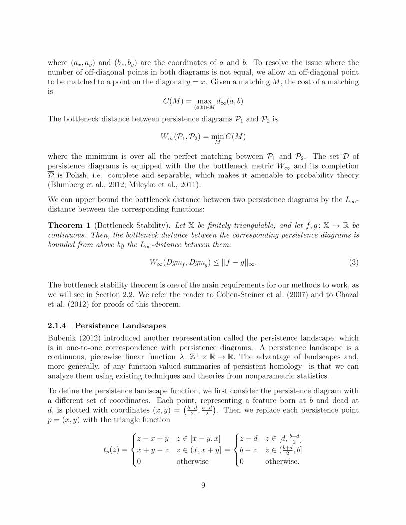
To define the persistence landscape function, we first consider the persistence diagram witha different set of coordinates. Each point, representing a feature born at b and dead atd, is plotted with coordinates (x, y) =

(b+d2, b−d

2

). Then we replace each persistence point

p = (x, y) with the triangle function

tp(z) =

z − x+ y z ∈ [x− y, x]

x+ y − z z ∈ (x, x+ y]

0 otherwise

=

z − d z ∈ [d, b+d

2]

b− z z ∈ ( b+d2, b]

0 otherwise.

9

0 2 4 6 8

02

46

8Persistence Diagram

Birth

Death

Landscape function

1 2 3 4 5 6 7 8

0.0

1.0

2.0

3.0

(Birth+Death)/2

(Death-Birth)/2

Figure 4: Left: a persistence diagrams with coordinates (birth, death). Right: the samepersistence diagram with coordinates ((birth+death)/2, (death-birth)/2). The red curveis the landscape λ(1, ·).

Notice that p is itself on the graph of tp(z). We obtain an arrangement of curves by overlayingthe graphs of the functions {tp(z)}p∈P ; see Figure 4.

The persistence landscape is defined formally as a walk through this arrangement:

λP(k, z) = kmaxp∈P

tp(z), (4)

where kmax is the kth maximum value in the set; in particular, 1max is the usual maxi-mum function. Observe that λP(k, z) is 1-Lipschitz.

For a fixed k ≥ 1 we define λ(·) := λ(k, ·). Let P be a probability distribution on the spaceof persistence landscapes upper bounded by T/2, for some T > 0. Let λ1, . . . , λn ∼ P . Wedefine the mean landscape as

µ(t) = E[λi(t)], t ∈ [0, T ].

The mean landscape is an unknown function that we would like to estimate. We estimate µwith the sample average

λn(t) =1

n

n∑i=1

λi(t), t ∈ [0, T ].

Note that since E(λn(t)) = µ(t), we have that λn is a point-wise unbiased estimator of theunknown function µ. Bubenik (2012) showed that λn converges pointwise to µ and that thepointwise Central Limit Theorem holds.

2.2 Research Plan

Several recent attempts have been made, with different approaches, to study persistencediagrams from a statistical point of view. See for example Turner et al. (2012); Robinson

10

and Turner (2013); Munch et al. (2013); Chazal et al. (2013c). In the following we describethe first results that we obtained in the study of persistence diagrams and other summaryfunctions, as well as the open questions that we propose to address.

2.2.1 Preliminary Work

In Fasy et al. (2013), Chazal et al. (2013a) and Chazal et al. (2013b), we have taken the firststeps towards a rigorous statistical analysis of persistent homology.

In particular, we have derived confidence sets for persistence diagrams that allow us toseparate topological signal from topological noise. An asymptotic 1 − α confidence set forthe bottleneck distance W∞(P ,P) is an interval [0, cn] such that

lim infn→∞

P(W∞(P ,P) ∈ [0, cn]

)≥ 1− α. (5)

We can visualize the confidence interval by centering a box of side length 2cn at each pointp on the persistence diagram. The point p is considered indistinguishable from noise if thecorresponding box, formally defined as {q ∈ R2 : d∞(p, q) ≤ cn}, intersects the diagonal.The union of boxes forms the confidence set for the unobserved persistence diagram P .Alternatively, we can visualize the confidence set by adding a band of width

√2cn around

the diagonal of the persistence diagram P . The interpretation is this: points in the bandare not significantly different from noise. Points above the band can be interpreted asrepresenting a significant topological feature. This leads to the diagrams shown in Figure 5.

●

●

●

●

●●

●

0 1 2 3 4 5 6

01

23

45

6

Persistence Diagram

Birth

Dea

th

●

●

●

●

●●

●

●

●

●

●

●●

●

●

●

●

●

●●

●

0 1 2 3 4 5 6

01

23

45

6

Persistence Diagram

Birth

Dea

th

●

●

●

●

●●

●

●

●

●

●

●●

●

noise

signal

Figure 5: First, we obtain the confidence interval [0, cn] for W∞(P,P). If a box of sidelength 2cn around a point in the diagram hits the diagonal, we consider that point to benoise. By putting a band of width

√2cn around the diagonal, we need only check which

points fall inside the band and outside the band. The plots show the two different ways torepresent the confidence interval [0, cn]. For this particular example cn = 0.5.

11

In Fasy et al. (2013) we proposed several methods for the construction of asymptotic confi-dence intervals for W∞(P ,P). The general strategy is as follows.

When f is the distance function (see Section 2.1.1), from the stability theorem (Theorem 1),we know that W∞(P , P) ≤ ‖dM − dSn‖∞. Hence, it suffices to find cn such that

lim infn→∞

P(‖dM − dSn‖∞ ∈ [0, cn]

)≥ 1− α (6)

to conclude thatlim infn→∞

P(W∞(P , P) ∈ [0, cn]

)≥ 1− α. (7)

Similarly when f is the density function ph (see Section 2.1.2), it suffices to find cn such that

lim infn→∞

P(‖ph − ph‖∞ ∈ [0, cn]

)≥ 1− α (8)

to conclude thatlim infn→∞

P(W∞(Ph, Ph) ∈ [0, cn]

)≥ 1− α. (9)

In the example of Figure 6 we use the bootstrap technique to construct an asymptotic 95%confidence set for the persistence diagram of the uniform density over the torus. We describedthis method in details in Chazal et al. (2013a).

Figure 6: We embed the torus S1×S1 in R3 and we use the rejection sampling algorithm ofDiaconis et al. (2012) (R = 1.5, r = 0.8) to sample 10, 000 points uniformly from the torus.Then, we compute the persistence diagram Ph using the Gaussian kernel with bandwidthh = 0.25 and use the bootstrap to construct the 0.95% confidence interval [0 , 0.01] forW∞(Ph,Ph). Note that the confidence set correctly captures the topology of the torus.That is, only the points representing real features of the torus are significantly far fromthe diagonal.

In Chazal et al. (2013b) we derived similar results for the landscape function, describedin Section 2.1.4). We showed that the average persistence landscape converges weakly to

12

a Gaussian process and we constructed 95% confidence bands for the average landscapeusing the multiplier bootstrap. A pair of functions `n, un : R → R is an asymptotic (1− α)confidence band for µ if, as n→∞,

P(`n(t) ≤ µ(t) ≤ un(t) for all t

)≥ 1− α, (10)

Confidence bands are valuable tools for statistical inference, as they allow to quantify andvisualize the uncertainty about the mean persistence landscape function µ and to screen outtopological noise. See Figure 7 for an example.

Figure 7: The plot on the left shows 8000 epicenters of earthquakes in the latitude/longituderectangle [−75, 75]× [−170, 10] of magnitude greater than 5.0 recorded between 1970 and2009 (USGS data). We randomly sampled m = 400 epicenters and computed the approxi-mated persistence diagram of the distance function (Betti 1). We repeated this proceduren = 30 times and computed the empirical average landscape λn. Using the multiplierbootstrap described in Chazal et al. (2013b), we obtained a uniform 95% confidence bandfor the average landscape µ(t) (right).

2.2.2 Research Aim

We will continue to study the objects and tools of persistent homology from a statisticalpoint of view. Our work will result in various non-parametric inferential procedures based onpersistence diagrams and summary functions such as persistence landscapes. These methodswill partially solve the important practical issue of approximating the persistent homologyin cases where exact computations are prohibitive.An immediate application of the confidence sets described above will be the formalization ofhypothesis tests that will be able to discriminate sampling artifacts (the topological noise)from the true topological features. More generally, we will treat diagrams as non-parametrictest statistics and, given two separate samples, we will study the power of tests that reject thenull hypothesis of population homogeneity solely based on homological features. Preliminaryresults on hypothesis tests for persistent homology are presented in Bubenik (2012) andRobinson and Turner (2013), although they are mainly based on permutation tests andthey do not provide a rigorous statistical analysis of the power of these procedures. We

13

will consider two non-parametric tests that have shown good performance in preliminaryexperiments: the Rosenbaum test (Rosenbaum, 2005) and Kernel Tests (Gretton et al.,2012). Tests of this kind will be extremely useful for instance in the medical imaging (Chunget al., 2009; Pachauri et al., 2011) and cosmology (Sousbie, 2011; van de Weygaert et al.,2011; Cisewski et al., 2014).

Much of the literature on computational topology focuses on using the distance function tothe data. As discussed in Bendich et al. (2011), such methods are quite sensitive to thepresence of outliers. In Fasy et al. (2013) we showed that density-based methods are morerobust: we can use the data to construct a smooth density estimator and then find thepersistence diagram defined by a filtration of the upper level sets of the density estimator.Another promising idea in this direction is the concept of distance of a measure to aset (Chazal et al., 2010). These functions share many properties with classical distancefunctions, which makes them suitable for inference purposes.

Another summary function for persistence diagrams can be obtained by modelling the dia-gram as a point process on the plane (see e.g. Daley and Vere-Jones, 2002). As described inEdelsbrunner et al. (2012) one can construct the empirical function on the plane φ : R2 → R,whose integral over every region A ⊂ R2 is the expected number of points in A. Alterna-tively, one can construct an intensity function, that is a smooth 2-dimensional densityestimation of the process on the plane. See Figure 8. We will derive a rigorous statisticalanalysis to prove the convergence in distribution of the average intensity function and tomeasure the significance of topological properties encoded in the corresponding persistencediagram.

Figure 8: We embed the torus S1 × S1 in R3 and we use the rejection sampling algorithmof Diaconis et al. (2012) (R = 5, r = 1.8) to sample 10,000 points uniformly from thetorus. Then we link it with a circle of radius 5, from which we sample 1,800 points. TheseN = 11, 800 points constitute the sample space (left). We randomly sample m = 600 ofthese points, estimate the corresponding persistence diagram (Betti 1) (middle left) andthe corresponding intensity function, using a Gaussian kernel with bandwidth h = 0.1(middle right). We repeat this procedure n = 30 times to construct the average intensityfunction (right).

Finally we will implement all the methods described above in a publicly available R package.

14

3 Density ClusteringThe other set of research objectives of this proposal pertains to the classic data-analytic taskof clustering in high dimensions. Suppose we observe a collection of points Sn = {X1, . . . , Xn}in RD. Density clustering allows us to identify and visualize the spatial organization of Sn,without specific knowledge about the data generating mechanism and in particular withoutany a priori information about the number of clusters.

3.1 Background

3.1.1 Level Set Trees

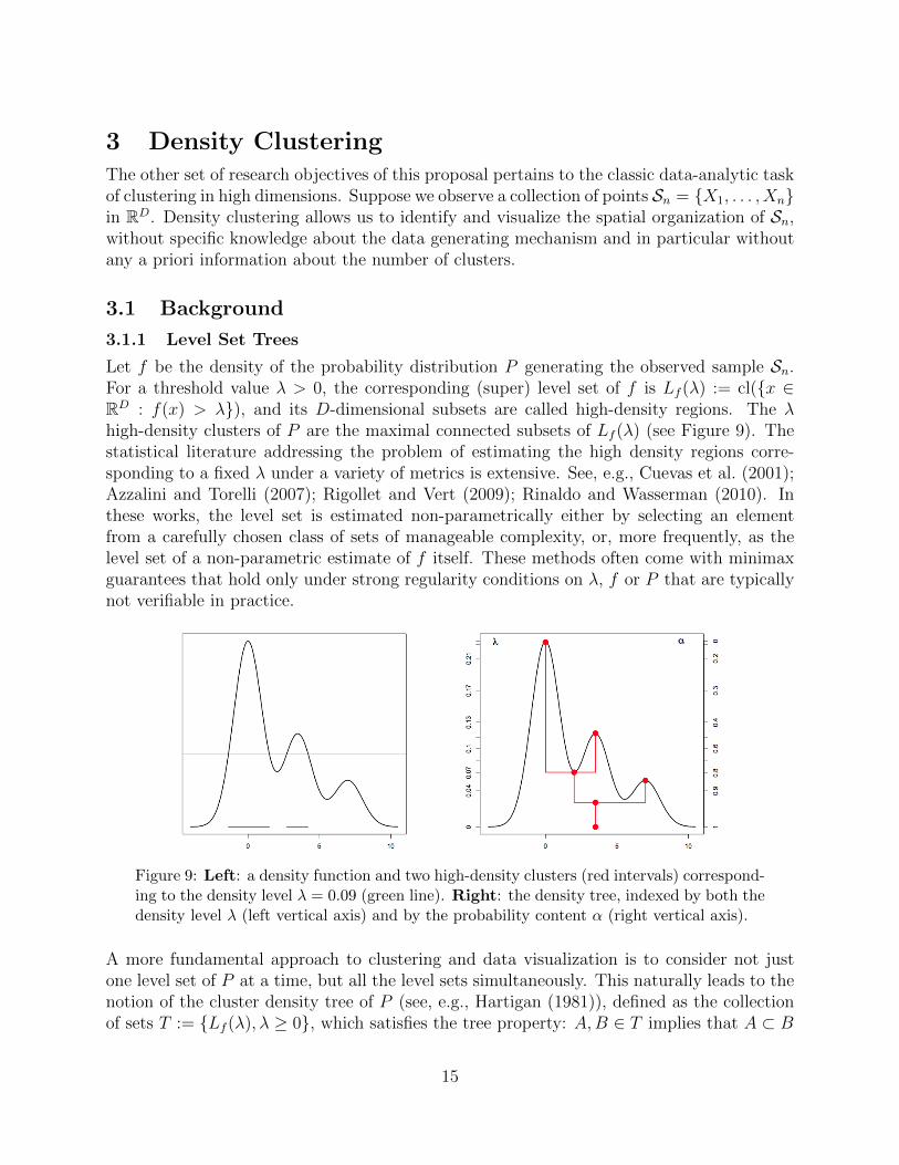
Let f be the density of the probability distribution P generating the observed sample Sn.For a threshold value λ > 0, the corresponding (super) level set of f is Lf (λ) := cl({x ∈RD : f(x) > λ}), and its D-dimensional subsets are called high-density regions. The λhigh-density clusters of P are the maximal connected subsets of Lf (λ) (see Figure 9). Thestatistical literature addressing the problem of estimating the high density regions corre-sponding to a fixed λ under a variety of metrics is extensive. See, e.g., Cuevas et al. (2001);Azzalini and Torelli (2007); Rigollet and Vert (2009); Rinaldo and Wasserman (2010). Inthese works, the level set is estimated non-parametrically either by selecting an elementfrom a carefully chosen class of sets of manageable complexity, or, more frequently, as thelevel set of a non-parametric estimate of f itself. These methods often come with minimaxguarantees that hold only under strong regularity conditions on λ, f or P that are typicallynot verifiable in practice.

Figure 9: Left: a density function and two high-density clusters (red intervals) correspond-ing to the density level λ = 0.09 (green line). Right: the density tree, indexed by both thedensity level λ (left vertical axis) and by the probability content α (right vertical axis).

A more fundamental approach to clustering and data visualization is to consider not justone level set of P at a time, but all the level sets simultaneously. This naturally leads to thenotion of the cluster density tree of P (see, e.g., Hartigan (1981)), defined as the collectionof sets T := {Lf (λ), λ ≥ 0}, which satisfies the tree property: A,B ∈ T implies that A ⊂ B

15

or B ⊂ A or A ∩ B = ∅. We will refer to this construction as the λ-tree. Alternatively, inRinaldo et al. (2012) the authors re-parametrize the depth of the tree by a probability contentparameter α ∈ (0, 1), and re-define the density α-tree as {L(α), α ∈ (0, 1)} where L(α) :=L(λα) with λα := sup{λ, P (Lf (λ)) ≥ α}. More recently, Kent et al. (2013) introducedthe cluster κ-tree, which facilitates the interpretation of the tree by precisely encoding theprobability content of each tree branch rather than density level. This new descriptor furtherimproves the interpretability and generality of level set trees.While the cluster density tree has long been known to be the most informative representationof P for the purposes of clustering, only very recently have statisticians and mathematiciansbegun to analyze it thoroughly (see, e.g., Stuetzle and Nugent (2010); Carlsson and Memoli(2010); Chaudhuri and Dasgupta (2010); Kpotufe and von Luxburg (2011); Rinaldo et al.(2012)), and much work remains to be done in order to understand the statistics of densitytrees.

3.2 Research Plan

The notion of density tree offers a principled way for visualizing a distribution in arbitrarydimensions and is clearly important for clustering. Many results have been published aboutclustering at a fixed density levels, but the first strong results about the accuracy of estima-tors for the entire level set tree appeared only recently (see Chaudhuri and Dasgupta (2010);Kpotufe and von Luxburg (2011); Rinaldo et al. (2012)). However a great deal of work re-mains to quantify the statistical properties of these methods. For example, the consistencyresults in Chaudhuri and Dasgupta (2010) and Kpotufe and von Luxburg (2011) are basedon the λ-tree. Since there is a one-to-one map between the levels of the λ-tree and those ofthe α-tree, it is likely that the α-tree is also consistent. We will also analyze the theoreticalproperties of the κ-tree, whose statistical consistency has never been studied before.

The cluster density tree can be seen as a topological descriptor. In order to study thestability of this object and to use it for statistical inference it is important to define adistance between two trees. In Morozov et al. (2013) the authors define the interleavingdistance, based on continuous maps between the trees, which leads to a stability results, butwhose cost of computation is prohibitive. Several definitions of distance are also presentedin Kent (2013). One of the most promising is the paint mover distance, which is basedon the Wasserstein metric and can be easily computed by solving a linear program. Wewill analyze the statistical properties of the paint mover distance and we will use it toconstruct an average tree that will lead to a rigorous definition of inferential procedures.A first step in this direction will consist in borrowing the concept of landscape functionfrom persistent homology. The idea is to summarize the information contained in the levelset tree using a continuous real valued function and then take advantage of its simplicityfor statistical inference. This procedure automatically defines a map from a d-dimensionaldensity to an unnormalized 1-dimensional density that preserves the critical value of theoriginal function. As done for the persistence landscape, we will construct an averagetree landscape and a confidence band, using appropriate bootstrapping procedure, which

16

Figure 10: We simulate 30 datasets, each of them formed by 300 points sampled from three2d-Gaussian distributions. The plot on the left shows one of these dataset. The plot in themiddle shows the cluster tree and corresponding tree landscape function (piecewise linearcurve). The plot on the right shows the empirical average landscape (black curve) obtainedas a pointwise average of the 30 Landscape functions. The pink band is a 95% confidenceband for µ(t), the mean Landscape associated to the sampling scheme. It is obtained usingthe multiplier bootstrap.

will lead to the formalization of hypothesis tests. See Figure 10 for a toy example withpreliminary results.

We will also try to extend these statistical techniques to a similar topological descriptor, theReeb graph. Given a continuous function f : X→ R defined on a triangulable topologicalspace X we consider the level set f−1(t) = {x ∈ X : f(x) = t}, for t ∈ R. Each levelset may contain several connected components. We say that two points x, y ∈ f−1(t) areequivalent, denoted by x ∼ y, if they are in the same connected component. The Reebgraph of the function f is the quotient space X/ ∼, which is the set of equivalence classesequipped with the quotient topology induced by this equivalence relation. Beside the levelsets of the function, the Reeb graph provides information on the topological space on whichthe function is defined. Even though the Reeb graph loses aspects of the original topologicalstructure, it can reflect the 1-dimensional connectivity of the space in some cases (Biasottiet al., 2008; Edelsbrunner and Harer, 2010; Bauer et al., 2013). See Figure 11 for an example.

Finally, a critical factor in the usefulness of a data analysis method is computational speedand memory efficiency. As in persistent homology, a rigorous statistical analysis of level settrees and Reeb graphs will allow us to approximate their construction in cases where exactcomputations are prohibitive.

17

Figure 11: Reeb graph of the height function of the torus.

ReferencesAdelchi Azzalini and Nicola Torelli. Clustering via nonparametric density estimation. Statis-

tics and Computing, 17(1):71–80, 2007.

Ulrich Bauer, Xiaoyin Ge, and Yusu Wang. Measuring distance between reeb graphs. arXivpreprint arXiv:1307.2839, 2013.

Paul Bendich, Taras Galkovskyi, and John Harer. Improving homology estimates with ran-dom walks. Inverse Problems, 27(12):124002, 2011.

Silvia Biasotti, Daniela Giorgi, Michela Spagnuolo, and Bianca Falcidieno. Reeb graphs forshape analysis and applications. Theoretical Computer Science, 392(1):5–22, 2008.

Andrew J Blumberg, Itamar Gal, Michael A Mandell, and Matthew Pancia. Persistenthomology for metric measure spaces, and robust statistics for hypothesis testing and con-fidence intervals. arXiv preprint arXiv:1206.4581, 2012.

Peter Bubenik. Statistical topology using persistence landscapes, 2012. arXiv preprint1207.6437.

Gunnar Carlsson. Topology and data. Bulletin of the American Mathematical Society, 46(2):255–308, 2009.

Gunnar Carlsson and Facundo Memoli. Multiparameter hierarchical clustering methods. InClassification as a Tool for Research, pages 63–70. Springer, 2010.

Kamalika Chaudhuri and Sanjoy Dasgupta. Rates of convergence for the cluster tree. InAdvances in Neural Information Processing Systems, pages 343–351, 2010.

Frederic Chazal, David Cohen-Steiner, Quentin Merigot, et al. Geometric inference formeasures based on distance functions. 2010.

Frederic Chazal, Vin de Silva, Marc Glisse, and Steve Oudot. The structure and stability ofpersistence modules. arXiv preprint arXiv:1207.3674, 2012.

18

Frederic Chazal, Brittany Terese Fasy, Fabrizio Lecci, Alessandro Rinaldo, Aarti Singh, andLarry Wasserman. On the bootstrap for persistence diagrams and landscapes, 2013a.arXiv preprint 1311.0376.

Frederic Chazal, Brittany Terese Fasy, Fabrizio Lecci, Alessandro Rinaldo, and Larry Wasser-man. Stochastic convergence of persistence landscapes and silhouettes, 2013b. arXivpreprint 1312.0308.

Frederic Chazal, Marc Glisse, Catherine Labruere, and Bertrand Michel. Optimal ratesof convergence for persistence diagrams in topological data analysis. arXiv preprintarXiv:1305.6239, 2013c.

Moo K Chung, Peter Bubenik, and Peter T Kim. Persistence diagrams of cortical surfacedata. In Information Processing in Medical Imaging, pages 386–397. Springer, 2009.

Jessi Cisewski, Rupert AC Croft, Peter E Freeman, Christopher R Genovese, NishikantaKhandai, Melih Ozbek, and Larry Wasserman. Nonparametric 3d map of the igm usingthe lyman-alpha forest. arXiv preprint arXiv:1401.1867, 2014.

David Cohen-Steiner, Herbert Edelsbrunner, and John Harer. Stability of persistence dia-grams. Discrete & Computational Geometry, 37(1):103–120, 2007.

Antonio Cuevas, Manuel Febrero, and Ricardo Fraiman. Cluster analysis: a further approachbased on density estimation. Computational Statistics & Data Analysis, 36(4):441–459,2001.

Vin de Silva and Robert Ghrist. Coverage in sensor networks via persistent homology.Algebraic & Geometric Topology, 7(339-358):24, 2007.

Persi Diaconis, Susan Holmes, and Mehrdad Shahshahani. Sampling from a manifold. arXivpreprint arXiv:1206.6913, 2012.

Herbert Edelsbrunner and John Harer. Persistent homology-a survey. Contemporary math-ematics, 453:257–282, 2008.

Herbert Edelsbrunner and John Harer. Computational Topology: An Introduction. AmerMathematical Society, 2010.

Herbert Edelsbrunner, A Ivanov, and R Karasev. Current open problems in discrete andcomputational geometry. 2012.

Brittany Fasy, Fabrizio Lecci, Alessandro Rinaldo, Larry Wasserman, Sivaraman Balakrish-nan, and Aarti Singh. Statistical inference for persistent homology, 2013. arXiv preprint1303.7117.

Jennifer Gamble and Giseon Heo. Exploring uses of persistent homology for statisticalanalysis of landmark-based shape data. Journal of Multivariate Analysis, 101(9):2184–2199, 2010.

19

Arthur Gretton, Karsten M Borgwardt, Malte J Rasch, Bernhard Scholkopf, and AlexanderSmola. A kernel two-sample test. The Journal of Machine Learning Research, 13:723–773,2012.

John A Hartigan. Consistency of single linkage for high-density clusters. Journal of theAmerican Statistical Association, 76(374):388–394, 1981.

Peter M Kasson, Afra Zomorodian, Sanghyun Park, Nina Singhal, Leonidas J Guibas, andVijay S Pande. Persistent voids: a new structural metric for membrane fusion. Bioinfor-matics, 23(14):1753–1759, 2007.

Brian Kent. Level Set Trees for Applied Statistics. PhD thesis, Department of Statistics,Carnegie Mellon University, 2013.

Brian P Kent, Alessandro Rinaldo, and Timothy Verstynen. Debacl: A python package forinteractive density-based clustering. arXiv preprint arXiv:1307.8136, 2013.

S. Kpotufe and U. von Luxburg. Pruning nearest neighbor cluster trees. In InternationalConference on Machine Learning (ICML), 2011.

Yuriy Mileyko, Sayan Mukherjee, and John Harer. Probability measures on the space ofpersistence diagrams. Inverse Problems, 27(12):124007, 2011.

Dmitriy Morozov, Kenes Beketayev, and Gunther Weber. Interleaving distance betweenmerge trees. In Workshop on Topological Methods in Data Analysis and Visualization:Theory, Algorithms and Applications (TopoInVis 13), 2013.

Elizabeth Munch, Paul Bendich, Katharine Turner, Sayan Mukherjee, Jonathan Mattingly,and John Harer. Probabilistic Frechet means and statistics on vineyards, 2013. arXivpreprint 1307.6530.

James R Munkres. Elements of algebraic topology, volume 2. Addison-Wesley Reading, 1984.

Deepti Pachauri, Chris Hinrichs, Moo K Chung, Sterling C Johnson, and Vikas Singh.Topology-based kernels with application to inference problems in alzheimer’s disease. Med-ical Imaging, IEEE Transactions on, 30(10):1760–1770, 2011.

Philippe Rigollet and Regis Vert. Optimal rates for plug-in estimators of density level sets.Bernoulli, 15(4):1154–1178, 2009.

Alessandro Rinaldo and Larry Wasserman. Generalized density clustering. The Annals ofStatistics, 38(5):2678–2722, 2010.

Alessandro Rinaldo, Aarti Singh, Rebecca Nugent, and Larry Wasserman. Stability ofdensity-based clustering. Journal of Machine Learning Research, 13:905–948, 2012.

Andrew Robinson and Katharine Turner. Hypothesis testing for topological data analysis.arXiv preprint arXiv:1310.7467, 2013.

20

Paul R Rosenbaum. An exact distribution-free test comparing two multivariate distribu-tions based on adjacency. Journal of the Royal Statistical Society: Series B (StatisticalMethodology), 67(4):515–530, 2005.

Thierry Sousbie. The persistent cosmic web and its filamentary structure–i. theory andimplementation. Monthly Notices of the Royal Astronomical Society, 414(1):350–383, 2011.

Werner Stuetzle and Rebecca Nugent. A generalized single linkage method for estimatingthe cluster tree of a density. Journal of Computational and Graphical Statistics, 19(2),2010.

Katharine Turner, Yuriy Mileyko, Sayan Mukherjee, and John Harer. Frechet means fordistributions of persistence diagrams, 2012. arXiv preprint 1206.2790.

Rien van de Weygaert, Gert Vegter, Herbert Edelsbrunner, Bernard JT Jones, PratyushPranav, Changbom Park, Wojciech A Hellwing, Bob Eldering, Nico Kruithof, EGP PatrickBos, et al. Alpha, betti and the megaparsec universe: on the topology of the cosmic web.In Transactions on Computational Science XIV, pages 60–101. Springer, 2011.

Afra Zomorodian and Gunnar Carlsson. Computing persistent homology. Discrete & Com-putational Geometry, 33(2):249–274, 2005.

Afra J Zomorodian. Topology for computing. Number 16. Cambridge University Press, 2005.

21