HAL Id: tel-02433613https://hal.inria.fr/tel-02433613v1

Submitted on 9 Jan 2020 (v1), last revised 21 Sep 2021 (v2)

HAL is a multi-disciplinary open accessarchive for the deposit and dissemination of sci-entific research documents, whether they are pub-lished or not. The documents may come fromteaching and research institutions in France orabroad, or from public or private research centers.

L’archive ouverte pluridisciplinaire HAL, estdestinée au dépôt et à la diffusion de documentsscientifiques de niveau recherche, publiés ou non,émanant des établissements d’enseignement et derecherche français ou étrangers, des laboratoirespublics ou privés.

Statistical Learning from Multimodal Genetic andNeuroimaging data for prediction of Alzheimer’s Disease

Pascal Lu

To cite this version:Pascal Lu. Statistical Learning from Multimodal Genetic and Neuroimaging data for prediction ofAlzheimer’s Disease. Statistics [math.ST]. Sorbonne Université, 2019. English. tel-02433613v1

Sorbonne Universite

École Doctorale d’Informatique, de Telecommunication et d’Électronique(ED130)

ARAMIS LAB a l’Institut du Cerveau et de laMoelle epiniere (UMR 7225)

Thèse de doctorat de Sorbonne Université

Spécialité: Informatique

Présentée par

Pascal LU

Pour obtenir de le grade de

Docteur de l’Université Sorbonne Université

Soutenue le 26 novembre 2019

Statistical Learning from Multimodal Genetic and Neuroimagingdata for prediction of Alzheimer’s Disease

Apprentissage Statistique à partir de Données Multimodales deGénétique et de Neuroimagerie pour la prédiction de la Maladie

d’Alzheimer

Rapporteurs

M. Christophe AMBROISE Professeur Université d’Évry Val-d’EssonneMme Agathe GUILLOUX Professeur Université d’Évry Val-d’Essonne

ExaminateursM. Jean-Daniel ZUCKER Directeur de recherche IRD, Sorbonne UniversitéM. Theodoros EVGENIOU Professeur INSEAD

Directeur de thèse

M. Olivier COLLIOT Directeur de recherche CNRS, ICM

1

3

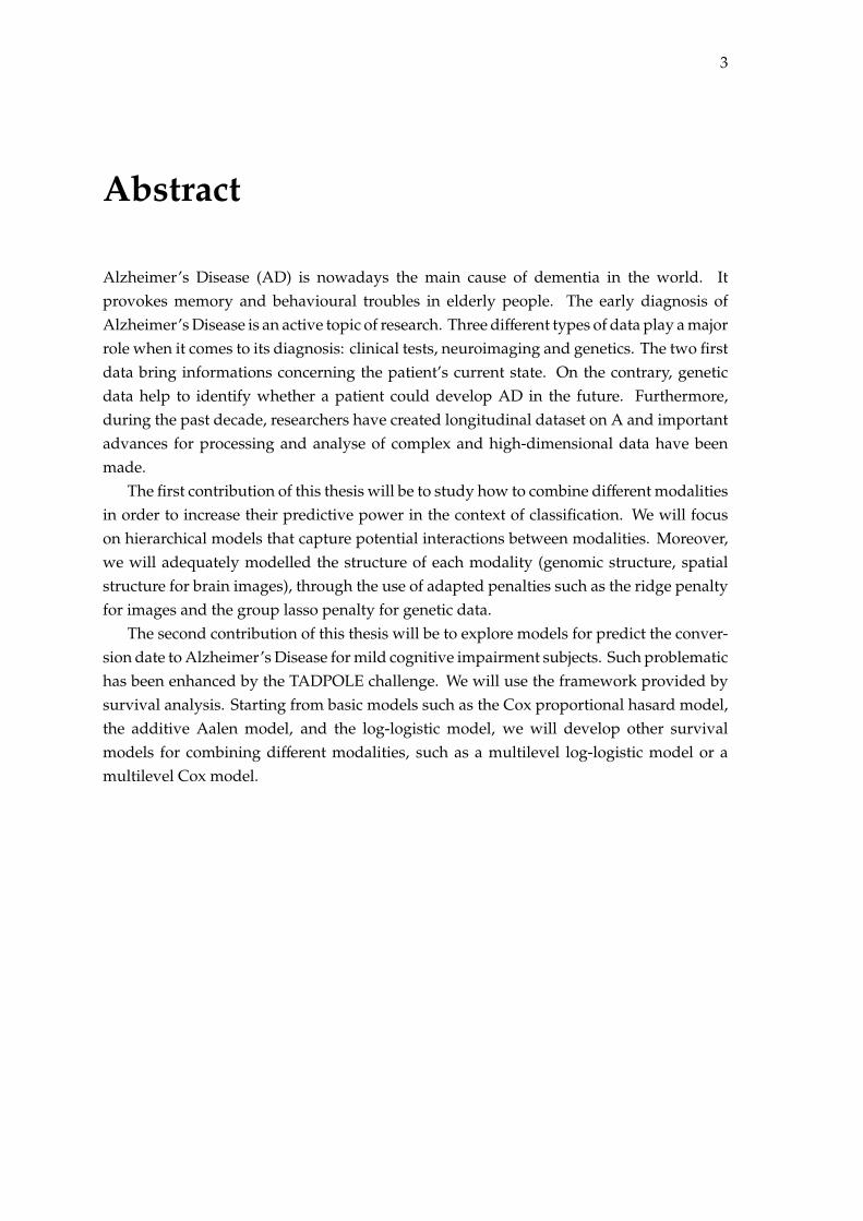
Abstract

Alzheimer’s Disease (AD) is nowadays the main cause of dementia in the world. Itprovokes memory and behavioural troubles in elderly people. The early diagnosis ofAlzheimer’s Disease is an active topic of research. Three different types of data play a majorrole when it comes to its diagnosis: clinical tests, neuroimaging and genetics. The two firstdata bring informations concerning the patient’s current state. On the contrary, geneticdata help to identify whether a patient could develop AD in the future. Furthermore,during the past decade, researchers have created longitudinal dataset on A and importantadvances for processing and analyse of complex and high-dimensional data have beenmade.

The first contribution of this thesis will be to study how to combine different modalitiesin order to increase their predictive power in the context of classification. We will focuson hierarchical models that capture potential interactions between modalities. Moreover,we will adequately modelled the structure of each modality (genomic structure, spatialstructure for brain images), through the use of adapted penalties such as the ridge penaltyfor images and the group lasso penalty for genetic data.

The second contribution of this thesis will be to explore models for predict the conver-sion date to Alzheimer’s Disease for mild cognitive impairment subjects. Such problematichas been enhanced by the TADPOLE challenge. We will use the framework provided bysurvival analysis. Starting from basic models such as the Cox proportional hasard model,the additive Aalen model, and the log-logistic model, we will develop other survivalmodels for combining different modalities, such as a multilevel log-logistic model or amultilevel Cox model.

5

Résumé

De nos jours, la maladie d’Alzheimer est la principale cause de démence. Elle provoque destroubles de mémoires et de comportements chez les personnes âgées. La diagnostic précocede la maladie d’Alzheimer est un sujet actif de recherche. Trois différents types de donnéesjouent un role particulier dans le diagnostic de la maladie d’Alzheimer: les tests cliniques,les données de neuroimagerie et les données génétiques. Les deux premières modalitésapportent de l’information concernant l’état actuel du patient. En revanche, les donnéesgénétiques permettent d’identifier si un patient est à risque et pourrait développer lamaladie d’Alzheimer dans le futur. Par ailleurs, durant la dernière décennie, les chercheursont crée des bases de données longitudinales sur la maladie d’Alzheimer et d’importantesrecherches ont été réalisées pour le traitement et l’analyse de données complexes en grandedimension.

La première contribution de cette thèse sera d’étudier comment combiner différentesmodalités dans le but d’améliorer leur pouvoir prédictif dans le contexte de la classifi-cation. Nous explorons les modèles multiniveaux permettant de capturer les potentiellesinteractions entre modalités. Par ailleurs, nous modéliserons la structure de chaque modal-ité (structure génétique, structure spatiale du cerveau) à travers l’utilisation de pénalitésadaptées comme la pénalité ridge pour les images, ou la pénalité group lasso pour lesdonnées génétiques.

La deuxième contribution de thèse sera d’explorer les modèles permettant de prédirela date de conversion à la maladie d’Alzheimer pour les patients atteints de troublescognitifs légers. De telles problématiques ont été mises en valeurs à travers de challenge,comme TADPOLE. Nous utiliserons principalement le cadre défini par les modèles desurvie. Partant de modèles classiques, comme le modèle d’hasard proportionnel de Cox,du modèle additif d’Aalen, et du modèle log-logistique, nous allons développer d’autresmodèles de survie pour la combinaisons de modalités, à travers un modèle log-logistiquemultiniveau ou un modèle de Cox multiniveau.

7

Remerciements

À mon directeur de thèse

Je tiens tout d’abord à remercier Olivier, mon directeur de thèse, pour m’avoir introduitau monde des données médicales, pour tout sa patience, ses remarques constructives toutau long de la thèse, et surtout sa grande disponibilité.

Aux membres du jury

Je souhaite remercier Theos que j’ai rencontré pendant ma première année de thèse. Jeretiendrais de nos échanges qu’il n’y a pas d’intérêt de faire des modèles complexes lorsqueles modèles les plus simples fonctionnent, et qu’il faut se poser la question si une équationmathématique a un sens physique.

Je tiens aussi à remercier Mme Agathe Guilloux et M. Christophe Ambroise, qui ontdéjà eu l’opportunité d’être jury du comité de suivi et donc de suivre mes travaux à desmoments très particuliers de la thèse, d’avoir aussi émis des remarques pertinentes etpermis de rectifier le tir lorsque c’était nécessaire.

Enfin, je remercie M. Jean-Daniel Zucker d’avoir accepté de faire parti du jury de thèse.Je suis honoré de pouvoir présenter mes travaux devant vous et de bénéficier de votreexpertise.

À l’équipe ARAMIS

L’équipe ARAMIS est une équipe sympathique et soudée avec qui j’ai passé trois bonnesannées. En particulier, j’ai pris beaucoup de plaisir à intégrer le club des Na, avec SimoNatoujours là à me surveiller, TiziaNa pour sa bonne humeur, Giulia BassignaNa, CataliNa,SabriNa, JuliaNa, EliNa et Federica(Na). Je voudrais remercier aussi mes voisins depalliers Jorge, Ludovic, Jérémy, Hao et Manon, pour toutes les astuces geek Alexandre R.et Benoît, mais aussi Raphaël, Maxime, Igor, Alexandre B., avec lesquels j’ai gardé un bonsouvenir de la soirée du gala de MICCAI 2017 à Québec, Wen, Marie-Constance, Fanny,Alexis, Arnaud(s), Adam, Baptiste, Vincent, Clémentine, Adam, Quentin, Paul, Dario,Emmanuelle, Ninon, Fabrizio, Benjamin, Stanley, Stéphane; Jean-Baptiste et Pietro lespremières personnes que j’ai connu à ARAMIS. J’ai aussi une pensée pour Anne Bertrandqui nous a quitté en 2018.

À mes parents

Pour tous leurs encouragements pendant toutes ces années.

9

Contents

Abstract 3

Résumé 7

Acknowledgements 7

Contents 9

List of Abbreviations 13

Introduction 15

I State of the art 19

1 Alzheimer’s Disease 211.1 Introduction . . . . . . . . . . . . . . . . . . . . . . . . . . . . . . . . . . . . . 211.2 Alzheimer’s Disease . . . . . . . . . . . . . . . . . . . . . . . . . . . . . . . . 21

1.2.1 Alzheimer’s Disease and the human brain . . . . . . . . . . . . . . . 221.2.2 Diagnostic of Alzheimer’s Disease . . . . . . . . . . . . . . . . . . . . 22

1.3 Modalities involved to study Alzheimer’s Disease . . . . . . . . . . . . . . . 231.3.1 Clinical and cognitive tests . . . . . . . . . . . . . . . . . . . . . . . . 231.3.2 Biological biomarkers . . . . . . . . . . . . . . . . . . . . . . . . . . . 25

1.3.2.1 Anatomical MRI . . . . . . . . . . . . . . . . . . . . . . . . . 251.3.2.2 PET scans . . . . . . . . . . . . . . . . . . . . . . . . . . . . . 251.3.2.3 Lumbar puncture . . . . . . . . . . . . . . . . . . . . . . . . 26

1.3.3 Genetic data . . . . . . . . . . . . . . . . . . . . . . . . . . . . . . . . . 261.4 Features . . . . . . . . . . . . . . . . . . . . . . . . . . . . . . . . . . . . . . . 27

1.4.1 Neuroimaging data . . . . . . . . . . . . . . . . . . . . . . . . . . . . . 271.4.2 Genetic data . . . . . . . . . . . . . . . . . . . . . . . . . . . . . . . . . 27

1.5 The Alzheimer’s Disease Neuroimaging Initiative (ADNI) dataset . . . . . . 301.5.1 Presentation . . . . . . . . . . . . . . . . . . . . . . . . . . . . . . . . . 301.5.2 Descriptive statistics of ADNI1 dataset . . . . . . . . . . . . . . . . . 301.5.3 MCI patients follow-up . . . . . . . . . . . . . . . . . . . . . . . . . . 32

1.6 Conclusion . . . . . . . . . . . . . . . . . . . . . . . . . . . . . . . . . . . . . . 33

2 Statistical and machine learning approaches for Imaging Genetics 352.1 Introduction . . . . . . . . . . . . . . . . . . . . . . . . . . . . . . . . . . . . . 35

10

2.2 Univariate and multivariate analyses between genetic and neuroimaging data 362.2.1 Univariate association between genotype and one phenotype trait . 372.2.2 Multivariate analyses . . . . . . . . . . . . . . . . . . . . . . . . . . . 39

2.2.2.1 Partial Least Squares . . . . . . . . . . . . . . . . . . . . . . 392.2.2.2 Linear regression between SNPs and neuroimaging data . . 402.2.2.3 Generative models . . . . . . . . . . . . . . . . . . . . . . . . 402.2.2.4 Pathways-based regression modelling . . . . . . . . . . . . 432.2.2.5 Epistasis effects and Random Forests on Distance Matrices 44

2.3 Combinaison of genetic and neuroimaging data for disease diagnosis . . . . 452.3.1 Dealing with high dimensional data . . . . . . . . . . . . . . . . . . . 472.3.2 Multiple Kernel Learning (MKL) . . . . . . . . . . . . . . . . . . . . . 482.3.3 Structured sparse regularisation . . . . . . . . . . . . . . . . . . . . . 50

2.4 Conclusion . . . . . . . . . . . . . . . . . . . . . . . . . . . . . . . . . . . . . . 51

3 Survival analysis: from theory to application for Alzheimer’s Disease 533.1 Introduction . . . . . . . . . . . . . . . . . . . . . . . . . . . . . . . . . . . . . 533.2 Background . . . . . . . . . . . . . . . . . . . . . . . . . . . . . . . . . . . . . 53

3.2.1 Assumptions . . . . . . . . . . . . . . . . . . . . . . . . . . . . . . . . 533.2.2 Censoring and truncation . . . . . . . . . . . . . . . . . . . . . . . . . 543.2.3 Survival and hazard function . . . . . . . . . . . . . . . . . . . . . . . 553.2.4 Kaplan-Meier and Nelson-Aalen estimators . . . . . . . . . . . . . . 563.2.5 Adding the covariates for individual predictions . . . . . . . . . . . . 57

3.2.5.1 Cox proportional hazard model . . . . . . . . . . . . . . . . 573.2.5.2 Exponential model . . . . . . . . . . . . . . . . . . . . . . . . 583.2.5.3 Log-logistic model . . . . . . . . . . . . . . . . . . . . . . . . 59

3.2.6 Model fitting . . . . . . . . . . . . . . . . . . . . . . . . . . . . . . . . 593.2.6.1 Parametric models . . . . . . . . . . . . . . . . . . . . . . . . 593.2.6.2 Semi-parametric models . . . . . . . . . . . . . . . . . . . . 60

3.2.7 Hypotheses behind the Cox proportional hazard model . . . . . . . . 613.3 Measuring the predictive value of a survival model . . . . . . . . . . . . . . 62

3.3.1 Median survival time . . . . . . . . . . . . . . . . . . . . . . . . . . . 623.3.2 Concordance-index (C-index) . . . . . . . . . . . . . . . . . . . . . . . 623.3.3 Cumulative AUC(t) . . . . . . . . . . . . . . . . . . . . . . . . . . . . 633.3.4 Kullback-Leibler divergence and Brier score . . . . . . . . . . . . . . 63

3.4 Combinaison of multimodal data using the Cox PH framework . . . . . . . 643.5 Illness-death models . . . . . . . . . . . . . . . . . . . . . . . . . . . . . . . . 663.6 Conclusion . . . . . . . . . . . . . . . . . . . . . . . . . . . . . . . . . . . . . . 67

II Contributions 69

4 Multilevel Modeling with Structured Penalties for Classification from ImagingGenetics Data 714.1 Introduction . . . . . . . . . . . . . . . . . . . . . . . . . . . . . . . . . . . . . 71

11

4.2 State of the art . . . . . . . . . . . . . . . . . . . . . . . . . . . . . . . . . . . . 724.3 Model set-up . . . . . . . . . . . . . . . . . . . . . . . . . . . . . . . . . . . . . 73

4.3.1 Multilevel Logistic Regression with Structured Penalties . . . . . . . 734.3.2 Minimization of S(W,βI,βI, β0) . . . . . . . . . . . . . . . . . . . . . 744.3.3 Probabilistic formulation . . . . . . . . . . . . . . . . . . . . . . . . . 76

4.4 Experimental results . . . . . . . . . . . . . . . . . . . . . . . . . . . . . . . . 774.4.1 Dataset . . . . . . . . . . . . . . . . . . . . . . . . . . . . . . . . . . . . 774.4.2 Results . . . . . . . . . . . . . . . . . . . . . . . . . . . . . . . . . . . . 774.4.3 Parameters . . . . . . . . . . . . . . . . . . . . . . . . . . . . . . . . . . 78

4.5 Conclusion . . . . . . . . . . . . . . . . . . . . . . . . . . . . . . . . . . . . . . 80

5 Contributions to the TADPOLE 2017-2022 challenge 835.1 Introduction . . . . . . . . . . . . . . . . . . . . . . . . . . . . . . . . . . . . . 835.2 Project details . . . . . . . . . . . . . . . . . . . . . . . . . . . . . . . . . . . . 83

5.2.1 Overview . . . . . . . . . . . . . . . . . . . . . . . . . . . . . . . . . . 835.2.2 Datasets . . . . . . . . . . . . . . . . . . . . . . . . . . . . . . . . . . . 845.2.3 Metrics . . . . . . . . . . . . . . . . . . . . . . . . . . . . . . . . . . . . 85

5.2.3.1 Multiclass Area Under the ROC Curve . . . . . . . . . . . . 855.2.3.2 Balanced Classification Accuracy . . . . . . . . . . . . . . . 86

5.3 Contributions . . . . . . . . . . . . . . . . . . . . . . . . . . . . . . . . . . . . 875.3.1 Disease progression paths . . . . . . . . . . . . . . . . . . . . . . . . . 875.3.2 Estimation of the conversion date to AD for MCI patients . . . . . . 88

5.4 Results and evaluation on D4 . . . . . . . . . . . . . . . . . . . . . . . . . . . 925.5 Conclusion . . . . . . . . . . . . . . . . . . . . . . . . . . . . . . . . . . . . . . 96

6 Multimodal survival models for predicting the conversion to Alzheimer’s Disease 976.1 Introduction . . . . . . . . . . . . . . . . . . . . . . . . . . . . . . . . . . . . . 976.2 Comparison between classification and survival analysis . . . . . . . . . . . 97

6.2.1 Models . . . . . . . . . . . . . . . . . . . . . . . . . . . . . . . . . . . . 986.2.2 Effect of covariates . . . . . . . . . . . . . . . . . . . . . . . . . . . . . 996.2.3 Assessment of the predictive value . . . . . . . . . . . . . . . . . . . . 1006.2.4 Conclusion . . . . . . . . . . . . . . . . . . . . . . . . . . . . . . . . . 101

6.3 A multilevel log-logistic model . . . . . . . . . . . . . . . . . . . . . . . . . . 1026.3.1 Motivation . . . . . . . . . . . . . . . . . . . . . . . . . . . . . . . . . . 1026.3.2 Parametrisation . . . . . . . . . . . . . . . . . . . . . . . . . . . . . . . 1046.3.3 Model fitting . . . . . . . . . . . . . . . . . . . . . . . . . . . . . . . . 1066.3.4 Experiments and results . . . . . . . . . . . . . . . . . . . . . . . . . . 1086.3.5 Discussion . . . . . . . . . . . . . . . . . . . . . . . . . . . . . . . . . . 111

6.4 Conclusion . . . . . . . . . . . . . . . . . . . . . . . . . . . . . . . . . . . . . . 112

7 Multilevel Cox Proportional hazard Model with Structured Penalties for ImagingGenetics data 1137.1 Introduction . . . . . . . . . . . . . . . . . . . . . . . . . . . . . . . . . . . . . 1137.2 State of the art . . . . . . . . . . . . . . . . . . . . . . . . . . . . . . . . . . . . 114

12

7.3 Methods . . . . . . . . . . . . . . . . . . . . . . . . . . . . . . . . . . . . . . . 1157.3.1 Model set-up . . . . . . . . . . . . . . . . . . . . . . . . . . . . . . . . 1157.3.2 Optimization . . . . . . . . . . . . . . . . . . . . . . . . . . . . . . . . 116

7.4 Experiments and results . . . . . . . . . . . . . . . . . . . . . . . . . . . . . . 1177.4.1 Dataset . . . . . . . . . . . . . . . . . . . . . . . . . . . . . . . . . . . . 1177.4.2 Evaluation . . . . . . . . . . . . . . . . . . . . . . . . . . . . . . . . . . 1177.4.3 Effect of cross-product covariates on conversion . . . . . . . . . . . . 119

7.5 Conclusion . . . . . . . . . . . . . . . . . . . . . . . . . . . . . . . . . . . . . . 120

Conclusion 123

Appendix 127

Scientific production 127

List of Figures 129

List of Tables 133

Bibliography 135

13

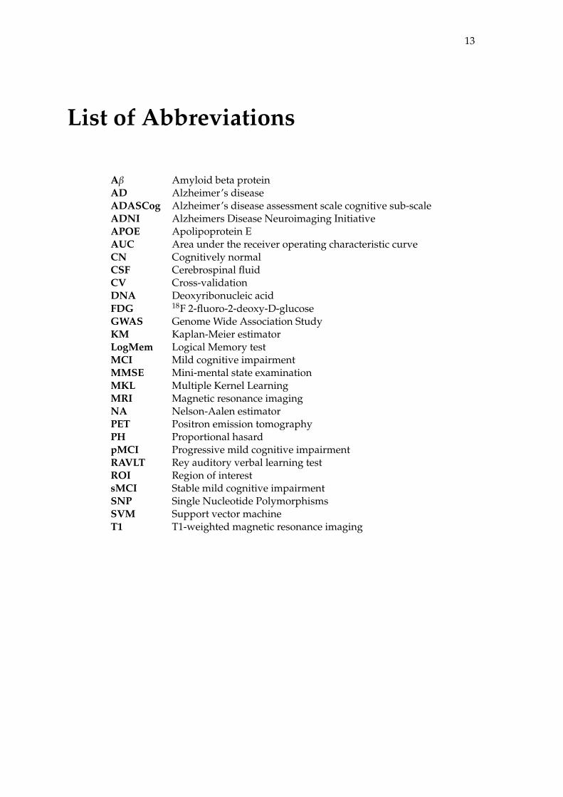
List of Abbreviations

Aβ Amyloid beta proteinAD Alzheimer’s diseaseADASCog Alzheimer’s disease assessment scale cognitive sub-scaleADNI Alzheimers Disease Neuroimaging InitiativeAPOE Apolipoprotein EAUC Area under the receiver operating characteristic curveCN Cognitively normalCSF Cerebrospinal fluidCV Cross-validationDNA Deoxyribonucleic acidFDG 18F 2-fluoro-2-deoxy-D-glucoseGWAS Genome Wide Association StudyKM Kaplan-Meier estimatorLogMem Logical Memory testMCI Mild cognitive impairmentMMSE Mini-mental state examinationMKL Multiple Kernel LearningMRI Magnetic resonance imagingNA Nelson-Aalen estimatorPET Positron emission tomographyPH Proportional hasardpMCI Progressive mild cognitive impairmentRAVLT Rey auditory verbal learning testROI Region of interestsMCI Stable mild cognitive impairmentSNP Single Nucleotide PolymorphismsSVM Support vector machineT1 T1-weighted magnetic resonance imaging

15

Introduction

Personalised medicine in the context of Alzheimer’s Disease

Personalised medicine aims at tailoring medical decisions, prevention and therapies toindividual patients, based on their predicted risk of disease, evolution and response. Inthis approach, patients are characterised using rich multimodal measurements (genomics,medical imaging, biomarkers. . .). A central challenge is then to develop predictive modelsfrom these measurements. To that end, it is necessary to design new statistical learningapproaches that can fully exploit the different types of data.

Neurodegenerative diseases, such as Alzheimer’s disease (AD), are complex multifac-torial diseases that represent major public health issues. In the context of these brain disor-ders, three types of data play a major role: genetics, neuroimaging and clinical tests. First,genetics allow identifying factors that modulate the risk of a given disease, its evolutionand response to treatment. It involves measurement of increasing complexity, from seriesof Single Nucleotide Polymorphisms (SNPs) provided by microarrays to high-throughputsequencing approaches such as whole-exome or even whole-genome sequencing. Second,neuroimaging allows measuring, in the living patient, different types of anatomical andfunctional alterations, using a variety of imaging modalities: anatomical, functional anddiffusion magnetic resonance imaging (MRI) and positron emission tomography (PET).Third, through clinical tests, the neurologist will assess the cognitive functions of the pa-tient, such as memory, attention or executive functions. Example of such tests are theMini-Mental State Exam (MMSE) and the ADAS-Cog test. Overall, both neuroimagingand clinical tests provide an accurate picture of the subject’s state.

Combining multimodal genetic and imaging data

Genetic and imaging technologies have witnessed considerable development during thepast 15 years. In the meantime, important advances have been made for processingand statistical analysis of these complex data. However, machine learning approachesthat can adequately integrate neuroimaging and genetic data are currently lacking. Thedevelopment of such approaches is particularly timely because massive datasets of patientswith both imaging and genetic data are now available. One can cite for instance theAlzheimer’s Disease Neuroimaging Initiative − ADNI (http://adni.loni.usc.edu), inthe context of AD.

Methodological developments are challenging because of:

(i) the high dimensionality of both types of data (around 105 or 106);

16

(ii) the complex multivariate interactions between variables. How can be we combinethese modalities in order to get a higher predictive power?

A large part of the literature on combination of imaging and genetic data focused onassociation studies, i.e. studying the relationships between genetic data in a univariateor multivariate manner. In such approaches, genetic is the time-independent variableand imaging the time-dependent variable. Univariate approaches follow the paradigmof so-called Genome-Wide Association Studies (GWAS) and look for statistical associa-tions between each individual SNP and each neuroimaging variable (for instance, averagewithin a brain region or value at a given voxel). However, SNPs often have weak effectswhen taken separately. Similarly, anatomical and functional brain phenotypes are bestdescribed using combinations of imaging variables. For that reason, researchers have pro-posed various types of multivariate approaches based for instance on penalized multipleregression, partial least squares or multivariate generative models.

A different question is to design statistical models that can predict the patient state (i.e.current or future diagnosis) from multimodal genetic and imaging data. Even though itis clinically relevant, this question has been the subject of less work in the literature. Onecan cite approaches based on regularized and sparse classification techniques as well asmultiple kernel learning. However, all these approaches put genetic and imaging data atthe same level while they could play different roles in the prediction. Indeed, imaging(or clinical) data provide a snapshot of the patient state at a given time while genetics canmodulate the evolution of the patient.

Statistical learning for prediction of Alzheimer’s disease

In the past decade, there has been intense research on the development of statistical learningmethods for predicting AD. Initial work has focused on automatic classification of patientswith AD and control subjects, in order to assist diagnosis. Such initial research has focusedon a single modality, using neuroimaging. A more challenging and useful aim is to predictthe future state of patients. In particular, many papers have been devoted to predictingthe future occurence of AD in patients with mild symptoms, a state called Mild CognitiveImpairment (MCI). Again, most of the approaches have used neuroimaging data as input,more rarely clinical tests and even more rarely multimodal data such as imaging andgenetic or clinical and genetic data. Moreover, they mostly tackled this question throughclassification approaches: one sets a fixed time window (for instance 3 years) and aimsto discriminate between MCI patients who will progress to AD within this time windowand those who will not. However, another clinically relevant question is to determinethe date at which the patient will develop AD. For instance, the care of the patient andthe information of the family (for instance for preparing institutionalization) can be quitedifferent depending on whether dementia is expected to develop within one year or fiveyears.

Introduction 17

Objectives of this PhD

The main objective of this PhD is to propose a methodological approaches to combinedifferent and genetic, neuroimaging and clinical modalities in order to predict the evolutionof patients to Alzheimer’s disease.

In the first part of this PhD, we aimed at predicting the current or future diagnosisof Alzheimer’s Disease using classification methods. In the state of the art, most modelscombine different modalities using an additive framework. Is it the best way to combinegenetics and neuroimaging data, although they do not provide the same level of informa-tion? Instead, we aimed to propose a multilevel framework that can capture interactionsbetween variables.

In a second part, we aimed at predicting the conversion date to Alzheimer’s Disease.Among the subjects who have Mild Cognitive Impairment (MCI), who are the patientswho will be affected by AD? if the patient converts, what is the conversion date? Ourdevelopments were performed within the framework of survival analysis, which is wellsuited to that purpose. Survival models provide a regression framework which directlyestimates the conversion date using only one time-point. Using cross-sectional data, in-stead of longitudinal data, is much more realistic from a medical point of view, althoughthe results in predictions will be less accurate. We applied different survival models to ourdata, such as the Cox proportional hasard model, the log-logistic model, and the Aalenadditive models. We also proposed modified versions of these models, using a multilevelframework.

The remainder of this document is organised as follows.The first part is devoted to the background and state-of-the-art. Chapter 1 provides

background information on AD and multimodal imaging, genetic and clinical data. It alsointroduces the ADNI database, a publicly available multicentric dataset that we will use forour experiments. Chapter 2 reviews existing statistical learning approaches for integrationof imaging and genetic data. Chapter 3 provides an overview of survival analysis andexisting applications to multimodal data and AD.

The second part of the document contains the contributions. Chapter 4 focuses on clas-sification techniques for assisting diagnosis of AD and predicting the future occurence ofAD in patients with MCI. In particular, we propose a multilevel framework for combiningimaging and genetic data. Chapter 5 presents our contribution to the TADPOLE inter-national challenge on prediction of AD. We used a standard survival model and rankedhigh on one of the challenge outcomes. Chapter 6 is focused on multimodal survivalmodels for prediction of AD. We first compare standard survival models and classificationapproaches. We then propose and evaluate an original multilevel log-logistic survivalmodel. In Chapter 7, we introduce a multilevel Cox Proportional Hazard model whichextends the approach proposed in Chapter 4 to the case of survival analysis.

19

Part I

State of the art

21

Chapter 1

Alzheimer’s Disease

1.1 Introduction

In this chapter, we provide a concise description of Alzheimer’s Disease (AD), from itsknown causes to its diagnosis. We will also describe the modalities that are involved inthe study of AD, such as neuropsychological tests, neuroimaging data, lumbar puncture,and genetic data; and how these modalities are preprocessed for statistical studies. Thischapter provides a short description of the ADNI dataset, that will be used throughout thiswork.

1.2 Alzheimer’s Disease

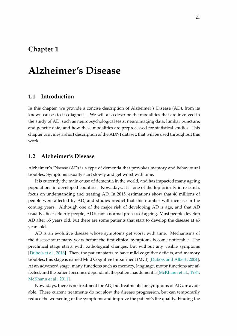
Alzheimer’s Disease (AD) is a type of dementia that provokes memory and behaviouraltroubles. Symptoms usually start slowly and get worst with time.

It is currently the main cause of dementia in the world, and has impacted many ageingpopulations in developed countries. Nowadays, it is one of the top priority in research,focus on understanding and treating AD. In 2015, estimations show that 46 millions ofpeople were affected by AD, and studies predict that this number will increase in thecoming years. Although one of the major risk of developing AD is age, and that ADusually affects elderly people, AD is not a normal process of ageing. Most people developAD after 65 years old, but there are some patients that start to develop the disease at 45years old.

AD is an evolutive disease whose symptoms get worst with time. Mechanisms ofthe disease start many years before the first clinical symptoms become noticeable. Thepreclinical stage starts with pathological changes, but without any visible symptoms[Dubois et al., 2016]. Then, the patient starts to have mild cognitive deficits, and memorytroubles; this stage is named Mild Cognitive Impairment (MCI) [Dubois and Albert, 2004].At an advanced stage, many functions such as memory, language, motor functions are af-fected, and the patient becomes dependant; the patient has dementia [McKhann et al., 1984,McKhann et al., 2011].

Nowadays, there is no treatment for AD, but treatments for symptoms of AD are avail-able. These current treatments do not slow the disease progression, but can temporarilyreduce the worsening of the symptoms and improve the patient’s life quality. Finding the

22

best cure for AD or a cure that can slower its development is currently a top priority in theresearch community.

1.2.1 Alzheimer’s Disease and the human brain

The humain brain is made up of 100 billion nerve cells, called neurones. Each neurone isconnected to several other neurones, and form all together a communication network. Agroup of neurones have a defined role, for instance there are groups for memory and learn-ing, and others for interactions with the environment (vision, feeling, hearing). Neuronesprocess and store the information, need energy, and communicate with each other.

Alzheimer’s Disease prevents neurones from functioning normally. The main causebehind Alzheimer’s Disease is not really known; what it is known is that some cells startby having malfunctions, and these malfunctions cause troubles and may affects otherneurones. The damage spreads to other cells, and progressively, neurones are unable towork properly and eventually die. These damage are irreversible.

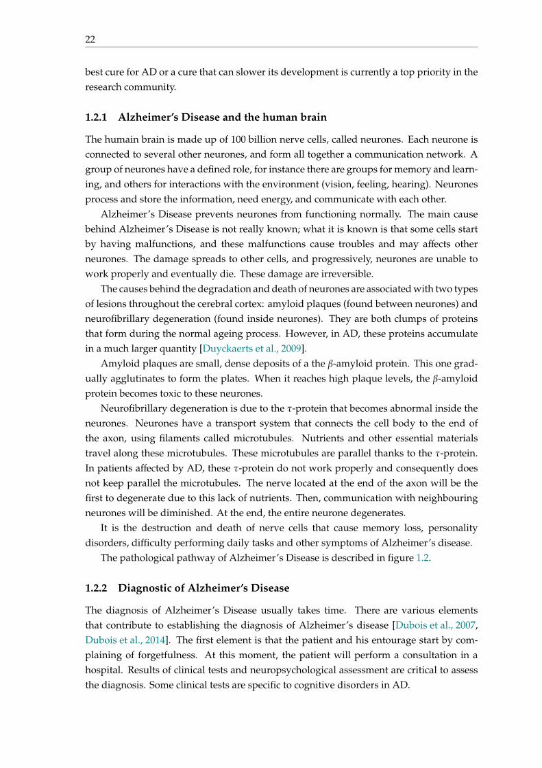
The causes behind the degradation and death of neurones are associated with two typesof lesions throughout the cerebral cortex: amyloid plaques (found between neurones) andneurofibrillary degeneration (found inside neurones). They are both clumps of proteinsthat form during the normal ageing process. However, in AD, these proteins accumulatein a much larger quantity [Duyckaerts et al., 2009].

Amyloid plaques are small, dense deposits of a the β-amyloid protein. This one grad-ually agglutinates to form the plates. When it reaches high plaque levels, the β-amyloidprotein becomes toxic to these neurones.

Neurofibrillary degeneration is due to the τ-protein that becomes abnormal inside theneurones. Neurones have a transport system that connects the cell body to the end ofthe axon, using filaments called microtubules. Nutrients and other essential materialstravel along these microtubules. These microtubules are parallel thanks to the τ-protein.In patients affected by AD, these τ-protein do not work properly and consequently doesnot keep parallel the microtubules. The nerve located at the end of the axon will be thefirst to degenerate due to this lack of nutrients. Then, communication with neighbouringneurones will be diminished. At the end, the entire neurone degenerates.

It is the destruction and death of nerve cells that cause memory loss, personalitydisorders, difficulty performing daily tasks and other symptoms of Alzheimer’s disease.

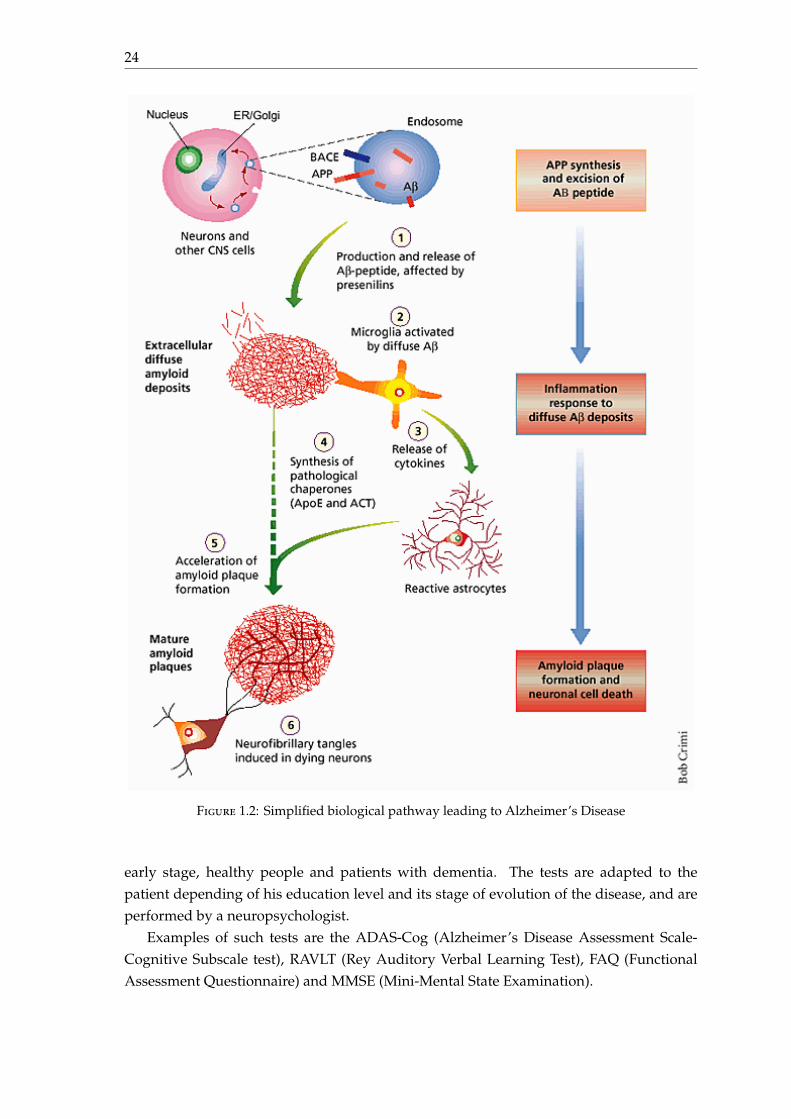
The pathological pathway of Alzheimer’s Disease is described in figure 1.2.

1.2.2 Diagnostic of Alzheimer’s Disease

The diagnosis of Alzheimer’s Disease usually takes time. There are various elementsthat contribute to establishing the diagnosis of Alzheimer’s disease [Dubois et al., 2007,Dubois et al., 2014]. The first element is that the patient and his entourage start by com-plaining of forgetfulness. At this moment, the patient will perform a consultation in ahospital. Results of clinical tests and neuropsychological assessment are critical to assessthe diagnosis. Some clinical tests are specific to cognitive disorders in AD.

1.3. Modalities involved to study Alzheimer’s Disease 23

Figure 1.1: Progression of Alzheimer’s Disease (reproduced fromhttps://www.brightfocus.org/alzheimers-disease/infographic/

progression-alzheimers-disease)

To complete the diagnosis, several analysis are made. The analysis of magnetic res-onance imaging (MRI) for anatomical and functional structure of the brain and Positronemission tomography scan (PET scan) for neuronal cell metabolism are performed to mea-sure the atrophy in vivo. The biological markers will support the neurologists’ hypothesis[Hampel et al., 2014].

1.3 Modalities involved to study Alzheimer’s Disease

1.3.1 Clinical and cognitive tests

The clinical and cognitive tests determine the patient’s cognitive disorders through a seriesof questions. These tests evaluate the memory and other cognitive functions such asorientation in space and time, language, comprehension, attention and reasoning. Thesecomprehensive tests distinguish between patients with Alzheimer’s Disease at a very

24

Figure 1.2: Simplified biological pathway leading to Alzheimer’s Disease

early stage, healthy people and patients with dementia. The tests are adapted to thepatient depending of his education level and its stage of evolution of the disease, and areperformed by a neuropsychologist.

Examples of such tests are the ADAS-Cog (Alzheimer’s Disease Assessment Scale-Cognitive Subscale test), RAVLT (Rey Auditory Verbal Learning Test), FAQ (FunctionalAssessment Questionnaire) and MMSE (Mini-Mental State Examination).

1.3. Modalities involved to study Alzheimer’s Disease 25

1.3.2 Biological biomarkers

On the contrary of clinical tests that aim at finding the existence of cognitive functiondisorders, biological biomarkers provide specific characteristic of the disease in vivo.

1.3.2.1 Anatomical MRI

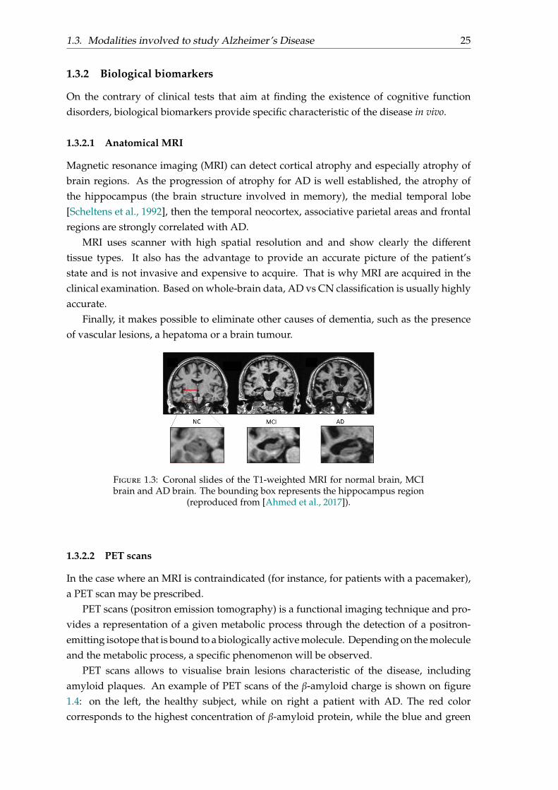
Magnetic resonance imaging (MRI) can detect cortical atrophy and especially atrophy ofbrain regions. As the progression of atrophy for AD is well established, the atrophy ofthe hippocampus (the brain structure involved in memory), the medial temporal lobe[Scheltens et al., 1992], then the temporal neocortex, associative parietal areas and frontalregions are strongly correlated with AD.

MRI uses scanner with high spatial resolution and and show clearly the differenttissue types. It also has the advantage to provide an accurate picture of the patient’sstate and is not invasive and expensive to acquire. That is why MRI are acquired in theclinical examination. Based on whole-brain data, AD vs CN classification is usually highlyaccurate.

Finally, it makes possible to eliminate other causes of dementia, such as the presenceof vascular lesions, a hepatoma or a brain tumour.

Figure 1.3: Coronal slides of the T1-weighted MRI for normal brain, MCIbrain and AD brain. The bounding box represents the hippocampus region

(reproduced from [Ahmed et al., 2017]).

1.3.2.2 PET scans

In the case where an MRI is contraindicated (for instance, for patients with a pacemaker),a PET scan may be prescribed.

PET scans (positron emission tomography) is a functional imaging technique and pro-vides a representation of a given metabolic process through the detection of a positron-emitting isotope that is bound to a biologically active molecule. Depending on the moleculeand the metabolic process, a specific phenomenon will be observed.

PET scans allows to visualise brain lesions characteristic of the disease, includingamyloid plaques. An example of PET scans of the β-amyloid charge is shown on figure1.4: on the left, the healthy subject, while on right a patient with AD. The red colorcorresponds to the highest concentration of β-amyloid protein, while the blue and green

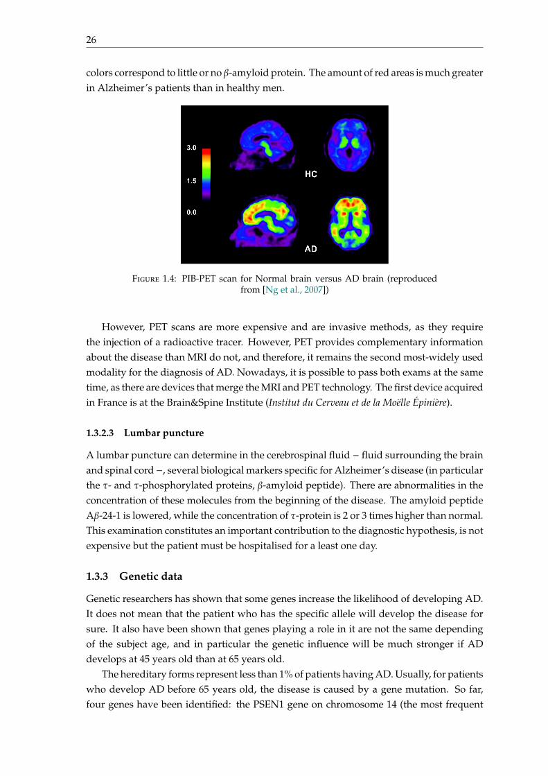
26

colors correspond to little or no β-amyloid protein. The amount of red areas is much greaterin Alzheimer’s patients than in healthy men.

Figure 1.4: PIB-PET scan for Normal brain versus AD brain (reproducedfrom [Ng et al., 2007])

However, PET scans are more expensive and are invasive methods, as they requirethe injection of a radioactive tracer. However, PET provides complementary informationabout the disease than MRI do not, and therefore, it remains the second most-widely usedmodality for the diagnosis of AD. Nowadays, it is possible to pass both exams at the sametime, as there are devices that merge the MRI and PET technology. The first device acquiredin France is at the Brain&Spine Institute (Institut du Cerveau et de la Moëlle Épinière).

1.3.2.3 Lumbar puncture

A lumbar puncture can determine in the cerebrospinal fluid − fluid surrounding the brainand spinal cord−, several biological markers specific for Alzheimer’s disease (in particularthe τ- and τ-phosphorylated proteins, β-amyloid peptide). There are abnormalities in theconcentration of these molecules from the beginning of the disease. The amyloid peptideAβ-24-1 is lowered, while the concentration of τ-protein is 2 or 3 times higher than normal.This examination constitutes an important contribution to the diagnostic hypothesis, is notexpensive but the patient must be hospitalised for a least one day.

1.3.3 Genetic data

Genetic researchers has shown that some genes increase the likelihood of developing AD.It does not mean that the patient who has the specific allele will develop the disease forsure. It also have been shown that genes playing a role in it are not the same dependingof the subject age, and in particular the genetic influence will be much stronger if ADdevelops at 45 years old than at 65 years old.

The hereditary forms represent less than 1% of patients having AD. Usually, for patientswho develop AD before 65 years old, the disease is caused by a gene mutation. So far,four genes have been identified: the PSEN1 gene on chromosome 14 (the most frequent

1.4. Features 27

case) [Janssen et al., 2000], the APP (Amyloid Precursor Protein) gene on chromosome 21(second incriminated in frequency), the PSEN2 gene on chromosome 1 or the gene calledSORL1 on chromosome 1. The genetic mutations provoke an increase in amyloid peptideproduction.

The sporadic forms are more frequent, and concern patients who develop AD after65 years old. The part of genetics is not predominant in the occurrence of the diseaseand other environmental factors come into play. AD can be considered as a multifactorialdisease. However, there are some genes of predisposition, such as the APOE4 gene locatedon chromosome 19 and involved in neuronal repair mechanisms.

Being a carrier of the allele ε4 of APOE4 (Apolipoprotein E) gene increases the riskof developing Alzheimer’s Disease by 11 times [Mahley et al., 2006]. However, thereare many people having this allele who will never declare the disease. In 2013, thelargest international study ever conducted on Alzheimer’s disease (International genomicsof Alzheimer project), identified eleven new regions of the genome involved in the occur-rence of this neurodegenerative disease and perhaps thirteen others, in validation course[Lambert et al., 2013].

Genetic data are collected using a DNA chip. A DNA chip contains millions of probesto which the genetic variants will hybridise and be detected by fluorescence.

1.4 Features

1.4.1 Neuroimaging data

Different types of features can be extracted from MRI data. The two most common arevoxel-based features (a measurement is taken at each voxel) and regional features (there isone measurement for each macroscopic region of the brain). We will work with regionalfeatures.

To extract such features, acquired MRI data need to be registered, normalised andcorrected. Images from and all subjects must be put in the same space, so that voxel-wisecorrespondence can be realised between subjects. Then an atlas is applied to parcelate thebrain into different regions. In our work, we used features extracted with the FreeSurfersoftware. The regional features represent the average cortical thickness in each region ofthe cortex and the volume of each subcortical region.

1.4.2 Genetic data

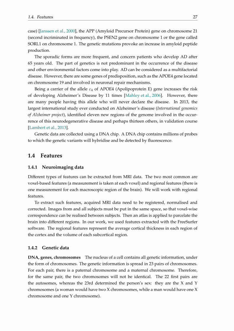
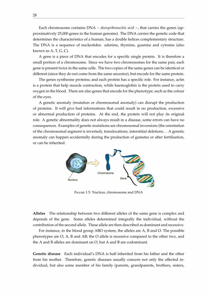
DNA, genes, chromosomes The nucleus of a cell contains all genetic information, underthe form of chromosomes. The genetic information is spread in 23 pairs of chromosomes.For each pair, there is a paternal chromosome and a maternal chromosome. Therefore,for the same pair, the two chromosomes will not be identical. The 22 first pairs arethe autosomes, whereas the 23rd determined the person’s sex: they are the X and Ychromosomes (a woman would have two X chromosomes, while a man would have one Xchromosome and one Y chromosome).

28

Each chromosome contains DNA − deoxyribonucleic acid −, that carries the genes (ap-proximatively 25,000 genes in the human genome). The DNA carries the genetic code thatdetermines the characteristics of a human, has a double helices complementary structure.The DNA is a sequence of nucleotides: adenine, thymine, guanine and cytosine (alsoknown as A, T, G, C).

A gene is a piece of DNA that encodes for a specific single protein. It is therefore asmall portion of a chromosome. Since we have two chromosomes for the same pair, eachgene is present twice in the same celle. The two copies of the same genes can be identical ordifferent (since they do not come from the same ancestor), but encode for the same protein.

The genes synthesise proteins; and each protein has a specific role. For instance, actinis a protein that help muscle contraction, while haemoglobin is the protein used to carryoxygen in the blood. There are also genes that encode for the phenotype, such as the colourof the eyes.

A genetic anomaly (mutation or chromosomal anomaly) can disrupt the productionof proteins. It will give bad informations that could result in no production, excessiveor abnormal production of proteins. At the end, the protein will not play its originalrole. A genetic abnormality does not always result in a disease, some errors can have noconsequences. Examples of genetic mutations are chromosomal inversions (the orientationof the chromosomal segment is inverted), translocations, interstitial deletions. . . A geneticanomaly can happen accidentally during the production of gametes or after fertilisation,or can be inherited.

Figure 1.5: Nucleus, chromosome and DNA

Alleles The relationship between two different alleles of the same gene is complex anddepends of the gene. Some alleles determined integrally the individual, without thecontribution of the second allele. These allele are then described as dominant and recessive.

For instance, in the blood group ABO system, the alleles are A, B and O. The possiblephenotypes are O, A, B and AB; the O allele is recessive compared to the other two, andthe A and B alleles are dominant on O, but A and B are codominant.

Genetic disease Each individual’s DNA is half inherited from his father and the otherfrom his mother. Therefore, genetic diseases usually concern not only the affected in-dividual, but also some member of his family (parents, grandparents, brothers, sisters,

1.4. Features 29

SNP 1 SNP 2 SNP 3 SNP 4 SNP 5 . . .DNA sequence from father C T G A A . . .

DNA sequence from mother C G G A C . . .

Table 1.1: Sequence of SNPs

major variant minor variantSNP 1 C ASNP 2 T GSNP 3 G CSNP 4 T ASNP 5 A C...

......

Table 1.2: Example of table defining major/minor variant in the entire pop-ulation

uncles, aunts. . .). A genetic disease is not always inherited, as there are several modes ofinheritance: autosomal dominant, autosomal recessive, X-linked.

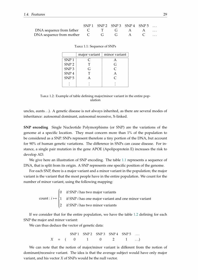
SNP encoding Single Nucleotide Polymorphisms (or SNP) are the variations of thegenome at a specific location. They must concern more than 1% of the population tobe considered as a SNP. SNPs represent therefore a tiny portion of the DNA, but accountfor 90% of human genetic variations. The difference in SNPs can cause disease. For in-stance, a single pair mutation in the gene APOE (Apolipoprotein E) increases the risk todevelop AD.

We give here an illustration of SNP encoding. The table 1.1 represents a sequence ofDNA, that is split from its origin. A SNP represents one specific position of the genome.

For each SNP, there is a major variant and a minor variant in the population; the majorvariant is the variant that the most people have in the entire population. We count for thenumber of minor variant, using the following mapping:

count : i 7→

0 if SNP i has two major variants

1 if SNP i has one major variant and one minor variant

2 if SNP i has two minor variants

If we consider that for the entire population, we have the table 1.2 defining for eachSNP the major and minor variant:

We can thus deduce the vector of genetic data:

SNP 1 SNP 2 SNP 3 SNP 4 SNP 5 . . .

X = ( 0 1 0 2 1 . . .)

We can note that the notion of major/minor variant is different from the notion ofdominant/recessive variant. The idea is that the average subject would have only majorvariant, and his vector X of SNPs would be the null vector.

30

Biological pathways The interactions between proteins (produced by genes) are complexand are usually expressed in terms of biological pathways. A biological pathway is aprocess through which proteins interact.

1.5 The Alzheimer’s Disease Neuroimaging Initiative (ADNI)dataset

1.5.1 Presentation

Presentation The Alzheimer’s Disease Neuroimaging Initiative (ADNI, http://adni.loni.usc.edu) collects data for modelling the progression of AD. Data includes cognitivetests, MRI and PET images, CSF, blood biomarkers and genetics. Data are collected, pre-processed, standardized, validated by ADNI. The current database on which researchersof ADNI are working on is the ADNI3 database. The ADNI3 database is built upon theADNI1, ADNI-GO, ADNI2 database.

ADNI1 dataset In this thesis, we will mainly work with the ADNI1 dataset. The ADNI1dataset − on the contrary of other ADNI datasets − provides a full SNP genotyping forsome subject. The number of SNPs that have been genotyped is around 620,901.

The ADNI1 dataset contains 819 patients with clinical scores, biological biomarkers andgenetic variants. Each patient is followed a for a certain time, and several and repeatedtimepoints are acquired through time. For each timepoint, are acquired clinical scoresand biological biomarkers, and the patient’s state is also given: cognitively normal (CN),early mild cognitive impairment (eMCI), late mild cognitive impairment (lMCI), SMC,dementia. Among the MCI subjects (eMCI + lMCI), we prefer to separate them into stableMCI (sMCI) and progressive MCI (MCI). Stable MCI at T means that the patient remainsMCI until at least date T, whereas pMCI means that the patient becomes AD before date T.

1.5.2 Descriptive statistics of ADNI1 dataset

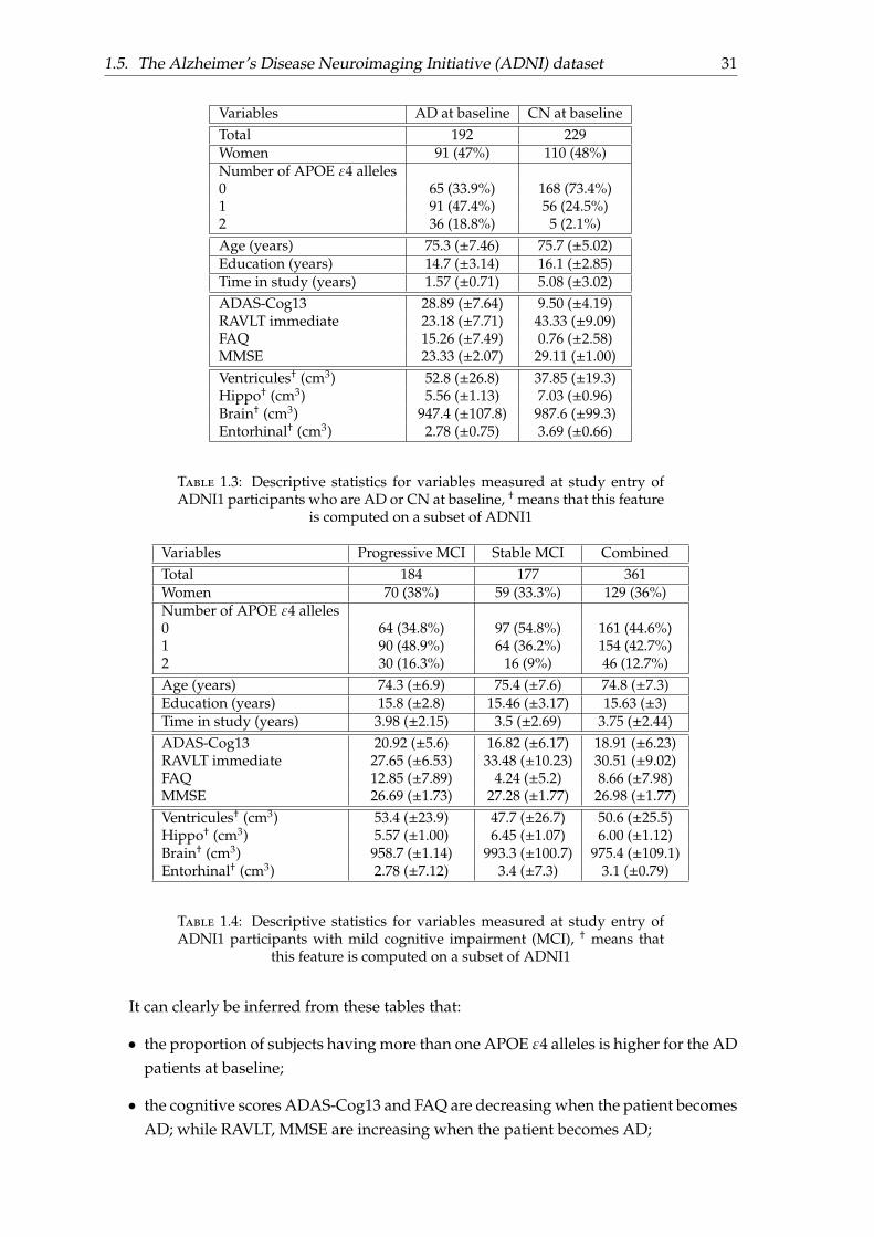
Tables 1.3 and 1.4 provide some descriptive statistics for variables measured at study entryof ADNI1 dataset.

Abbreviations used for biological biomarkers are:

• Mid-Temp for the volume of middle temporal gyrus, calculated from medical reso-nance images;

• Hippo for the volume of hippocampi, calculated from medical resonance images;

• Brain for the volume of the whole brain, calculated from medical resonance images;

• Entorhinal for the volume of the entorhinal region, calculated from medical resonanceimages;

• FDG for the sum of mean glucose metabolism uptake in regions of angular, temporal,and posterior cingulate, calculated from PET scans;

1.5. The Alzheimer’s Disease Neuroimaging Initiative (ADNI) dataset 31

Variables AD at baseline CN at baselineTotal 192 229Women 91 (47%) 110 (48%)Number of APOE ε4 alleles0 65 (33.9%) 168 (73.4%)1 91 (47.4%) 56 (24.5%)2 36 (18.8%) 5 (2.1%)Age (years) 75.3 (±7.46) 75.7 (±5.02)Education (years) 14.7 (±3.14) 16.1 (±2.85)Time in study (years) 1.57 (±0.71) 5.08 (±3.02)ADAS-Cog13 28.89 (±7.64) 9.50 (±4.19)RAVLT immediate 23.18 (±7.71) 43.33 (±9.09)FAQ 15.26 (±7.49) 0.76 (±2.58)MMSE 23.33 (±2.07) 29.11 (±1.00)Ventricules† (cm3) 52.8 (±26.8) 37.85 (±19.3)Hippo† (cm3) 5.56 (±1.13) 7.03 (±0.96)Brain† (cm3) 947.4 (±107.8) 987.6 (±99.3)Entorhinal† (cm3) 2.78 (±0.75) 3.69 (±0.66)

Table 1.3: Descriptive statistics for variables measured at study entry ofADNI1 participants who are AD or CN at baseline, † means that this feature

is computed on a subset of ADNI1

Variables Progressive MCI Stable MCI CombinedTotal 184 177 361Women 70 (38%) 59 (33.3%) 129 (36%)Number of APOE ε4 alleles0 64 (34.8%) 97 (54.8%) 161 (44.6%)1 90 (48.9%) 64 (36.2%) 154 (42.7%)2 30 (16.3%) 16 (9%) 46 (12.7%)Age (years) 74.3 (±6.9) 75.4 (±7.6) 74.8 (±7.3)Education (years) 15.8 (±2.8) 15.46 (±3.17) 15.63 (±3)Time in study (years) 3.98 (±2.15) 3.5 (±2.69) 3.75 (±2.44)ADAS-Cog13 20.92 (±5.6) 16.82 (±6.17) 18.91 (±6.23)RAVLT immediate 27.65 (±6.53) 33.48 (±10.23) 30.51 (±9.02)FAQ 12.85 (±7.89) 4.24 (±5.2) 8.66 (±7.98)MMSE 26.69 (±1.73) 27.28 (±1.77) 26.98 (±1.77)Ventricules† (cm3) 53.4 (±23.9) 47.7 (±26.7) 50.6 (±25.5)Hippo† (cm3) 5.57 (±1.00) 6.45 (±1.07) 6.00 (±1.12)Brain† (cm3) 958.7 (±1.14) 993.3 (±100.7) 975.4 (±109.1)Entorhinal† (cm3) 2.78 (±7.12) 3.4 (±7.3) 3.1 (±0.79)

Table 1.4: Descriptive statistics for variables measured at study entry ofADNI1 participants with mild cognitive impairment (MCI), † means that

this feature is computed on a subset of ADNI1

It can clearly be inferred from these tables that:

• the proportion of subjects having more than one APOE ε4 alleles is higher for the ADpatients at baseline;

• the cognitive scores ADAS-Cog13 and FAQ are decreasing when the patient becomesAD; while RAVLT, MMSE are increasing when the patient becomes AD;

32

• the ventricule volume is much larger for patients having AD than for control patients,whereas the hippocampi is smaller for patients having AD than for control patients.

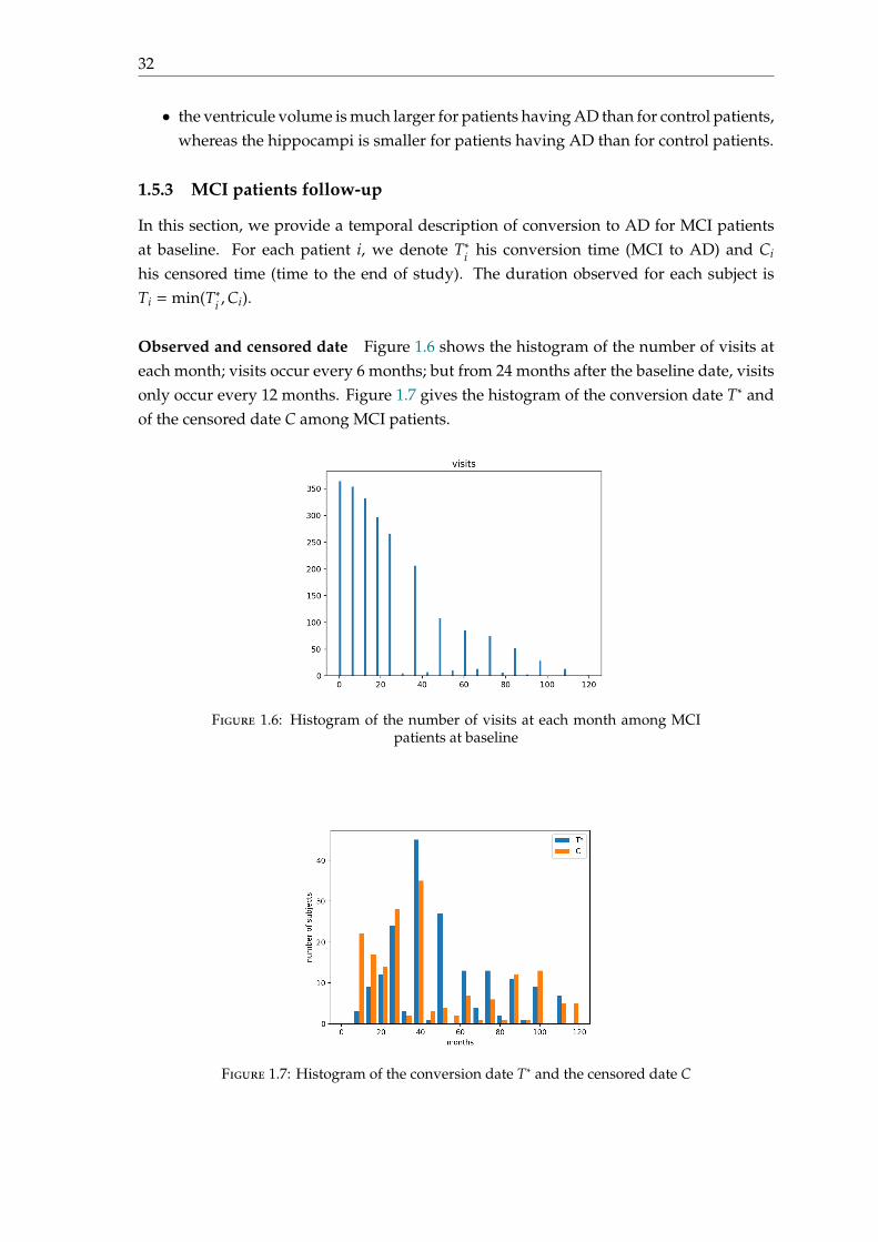
1.5.3 MCI patients follow-up

In this section, we provide a temporal description of conversion to AD for MCI patientsat baseline. For each patient i, we denote T∗i his conversion time (MCI to AD) and Ci

his censored time (time to the end of study). The duration observed for each subject isTi = min(T∗i ,Ci).

Observed and censored date Figure 1.6 shows the histogram of the number of visits ateach month; visits occur every 6 months; but from 24 months after the baseline date, visitsonly occur every 12 months. Figure 1.7 gives the histogram of the conversion date T∗ andof the censored date C among MCI patients.

Figure 1.6: Histogram of the number of visits at each month among MCIpatients at baseline

Figure 1.7: Histogram of the conversion date T∗ and the censored date C

1.6. Conclusion 33

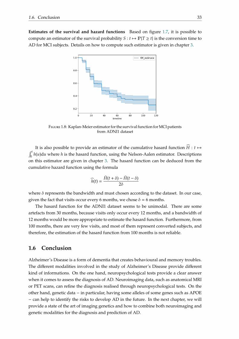
Estimates of the survival and hazard functions Based on figure 1.7, it is possible tocompute an estimator of the survival probability S : t 7→ PT ≥ t is the conversion time toAD for MCI subjects. Details on how to compute such estimator is given in chapter 3.

Figure 1.8: Kaplan-Meier estimator for the survival function for MCI patientsfrom ADNI1 dataset

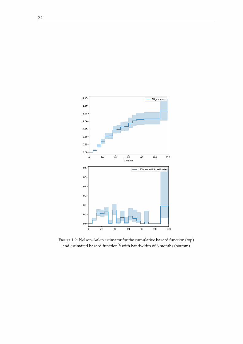
It is also possible to provide an estimator of the cumulative hasard function H : t 7→∫ t0 h(u)du where h is the hasard function, using the Nelson-Aalen estimator. Descriptions

on this estimator are given in chapter 3. The hasard function can be deduced from thecumulative hazard function using the formula

h(t) =H(t + δ) − H(t − δ)

2δ

where δ represents the bandwidth and must chosen according to the dataset. In our case,given the fact that visits occur every 6 months, we chose δ = 6 months.

The hasard function for the ADNI1 dataset seems to be unimodal. There are someartefacts from 30 months, because visits only occur every 12 months, and a bandwidth of12 months would be more appropriate to estimate the hasard function. Furthermore, from100 months, there are very few visits, and most of them represent converted subjects, andtherefore, the estimation of the hasard function from 100 months is not reliable.

1.6 Conclusion

Alzheimer’s Disease is a form of dementia that creates behavioural and memory troubles.The different modalities involved in the study of Alzheimer’s Disease provide differentkind of informations. On the one hand, neuropsychological tests provide a clear answerwhen it comes to assess the diagnosis of AD. Neuroimaging data, such as anatomical MRIor PET scans, can refine the diagnosis realised through neuropsychological tests. On theother hand, genetic data − in particular, having some alleles of some genes such as APOE− can help to identify the risks to develop AD in the future. In the next chapter, we willprovide a state of the art of imaging genetics and how to combine both neuroimaging andgenetic modalities for the diagnosis and prediction of AD.

34

Figure 1.9: Nelson-Aalen estimator for the cumulative hazard function (top)and estimated hazard function h with bandwidth of 6 months (bottom)

35

Chapter 2

Statistical and machine learningapproaches for Imaging Genetics

2.1 Introduction

In this chapter, we provide a review of the state of the art in Imaging Genetics [Liu and Calhoun, 2014]and its applications to Alzheimer’s Disease. Imaging Genetic studies the relation betweengenetic variations and individual endophenotypes such as neuroimages. The informationprovided by endophenotypes is closer to the biology of genetic function than the clinicalphenotype (disease diagnosis).

This research area focuses on the influence of genes on brain and its pathologies. Usingthe information from neuroimages and genetics, it try to determine which differences inSNPs can lead to brain pathologies. The main idea behind imaging genetics is that commonvariants in SNPs lead to common diseases.

The first topic of research in imaging genetics is to study the association between geneticand brain imaging data, using a univariate or multivariate approach. A univariate analysiswill associate the genotype to one specific phenotype trait, whereas a multivariate anal-ysis will associate the genotype to several phenotype traits such as a whole neuroimage.Example of multivariate approaches are the partial least squares [Laird and Lange, 2011],the sparse canonical correlation analysis [Du et al., 2014], the sparse regularised linear re-gression with a ℓ1-penalty [Kohannim et al., 2012a], the use of the group lasso penalty[Silver et al., 2012, Silver and Montana, 2012], or a Bayesian modeling that links geneticvariants to imaging regions and imaging regions [Chekouo et al., 2016, Batmanghelich et al., 2016].In these three last examples, the authors consider that the endophenotype can be explainedas a sum of effects from genetic variants.

The second topic of research in imaging genetics is to combine these two differentmodalities (imaging and genetics) for automatic classification or disease evolution of pa-tients. Researchers using such approach consider that the genotype and the neuroimagesprovide complementary information concerning the subject’s disease state, or that know-ing the genotype can help to refine the diagnosis using only the imaging modality. In[Wang et al., 2012, Peng et al., 2016] for instance, the authors uses machine learning meth-ods to build predictors for Alzheimer’s disease (AD) diagnosis. The main challenges inthis topic of research is that the heterogeneous nature of data, and the way both imagingand genetics can be combined efficiently.

36

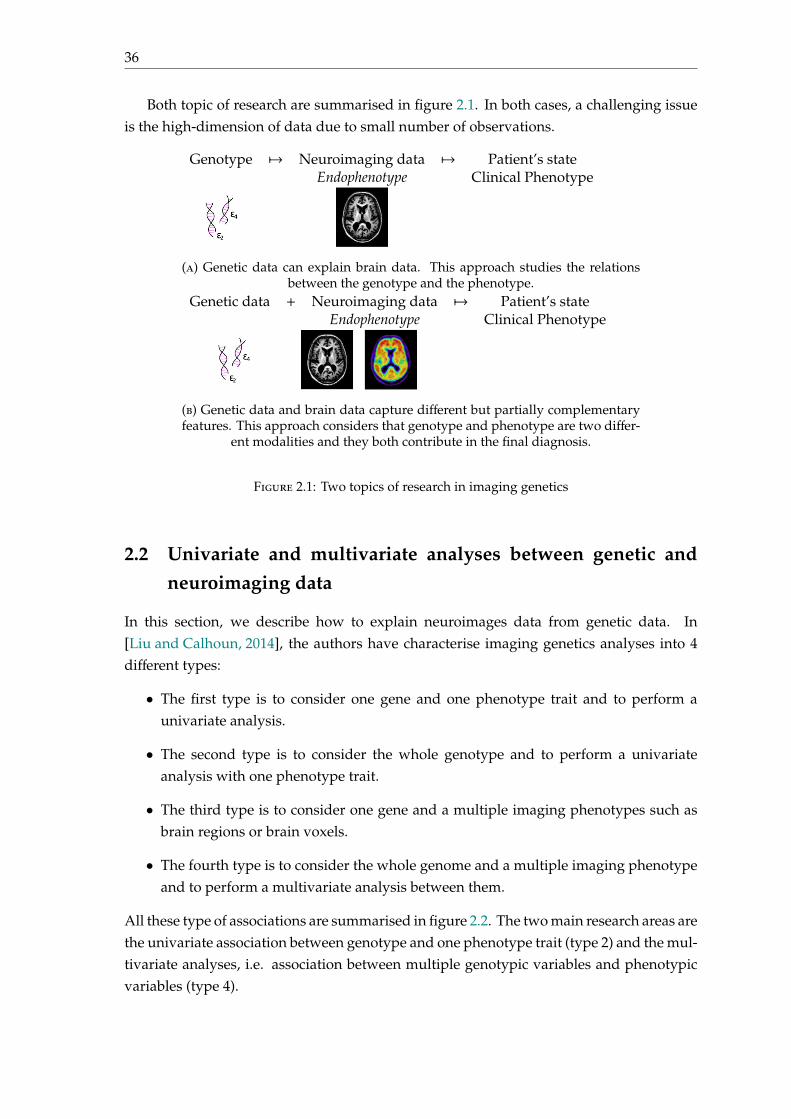
Both topic of research are summarised in figure 2.1. In both cases, a challenging issueis the high-dimension of data due to small number of observations.

Genotype 7→ Neuroimaging data 7→ Patient’s stateEndophenotype Clinical Phenotype

(a) Genetic data can explain brain data. This approach studies the relationsbetween the genotype and the phenotype.

Genetic data + Neuroimaging data 7→ Patient’s stateEndophenotype Clinical Phenotype

(b) Genetic data and brain data capture different but partially complementaryfeatures. This approach considers that genotype and phenotype are two differ-

ent modalities and they both contribute in the final diagnosis.

Figure 2.1: Two topics of research in imaging genetics

2.2 Univariate and multivariate analyses between genetic andneuroimaging data

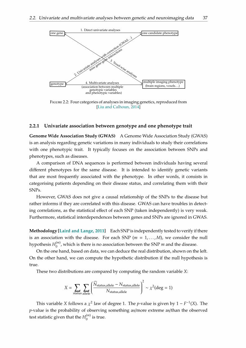
In this section, we describe how to explain neuroimages data from genetic data. In[Liu and Calhoun, 2014], the authors have characterise imaging genetics analyses into 4different types:

• The first type is to consider one gene and one phenotype trait and to perform aunivariate analysis.

• The second type is to consider the whole genotype and to perform a univariateanalysis with one phenotype trait.

• The third type is to consider one gene and a multiple imaging phenotypes such asbrain regions or brain voxels.

• The fourth type is to consider the whole genome and a multiple imaging phenotypeand to perform a multivariate analysis between them.

All these type of associations are summarised in figure 2.2. The two main research areas arethe univariate association between genotype and one phenotype trait (type 2) and the mul-tivariate analyses, i.e. association between multiple genotypic variables and phenotypicvariables (type 4).

2.2. Univariate and multivariate analyses between genetic and neuroimaging data 37

one gene

genotype

one candidate phenotype

multiple imaging phenotype(brain regions, voxels. . .)

1. Direct univariate analyses

2. Univariate analyses with

correctio

n (GWAS. ..)

missgene-gene interactio

ns

3. Voxel-wise analyses

4. Multivariate analyses(association between multiple

genotypic variablesand phenotypic variables)

Figure 2.2: Four categories of analyses in imaging genetics, reproduced from[Liu and Calhoun, 2014]

2.2.1 Univariate association between genotype and one phenotype trait

Genome Wide Association Study (GWAS) A Genome Wide Association Study (GWAS)is an analysis regarding genetic variations in many individuals to study their correlationswith one phenotypic trait. It typically focuses on the association between SNPs andphenotypes, such as diseases.

A comparison of DNA sequences is performed between individuals having severaldifferent phenotypes for the same disease. It is intended to identify genetic variantsthat are most frequently associated with the phenotype. In other words, it consists incategorising patients depending on their disease status, and correlating them with theirSNPs.

However, GWAS does not give a causal relationship of the SNPs to the disease butrather informs if they are correlated with this disease. GWAS can have troubles in detect-ing correlations, as the statistical effect of each SNP (taken independently) is very weak.Furthermore, statistical interdependences between genes and SNPs are ignored in GWAS.

Methodology [Laird and Lange, 2011] Each SNP is independently tested to verify if thereis an association with the disease. For each SNP (m = 1, . . . ,M), we consider the nullhypothesis H(m)

0 , which is there is no association between the SNP m and the disease.On the one hand, based on data, we can deduce the real distribution, shown on the left.

On the other hand, we can compute the hypothetic distribution if the null hypothesis istrue.

These two distributions are compared by computing the random variable X:

X =∑

status

∑allele

Nstatus,allele −Nstatus,allele

Nstatus,allele

2

∼ χ2(deg = 1)

This variable X follows a χ2 law of degree 1. The p-value is given by 1 − F−1(X). Thep-value is the probability of observing something as/more extreme as/than the observedtest statistic given that the H(m)

0 is true.

38

Real distribution Hypothetic distribution if H(m)0 holds

Allele A Allele a Allele A Allele aCN NA,CN Na,CN NCN CN NA,CN =

NANCNN Na,CN =

NaNCNN NCN

AD NA,AD Na,AD NAD AD NA,AD =NANAD

N Na,AD =NaNAD

N NADNA Na N NA Na N

Figure 2.3: Real vs hypothetic distribution (N is the number of subjects, NA(resp. Na) the number of subjects with allele A (resp. a), NCN (resp. NAD) the

number of subjects who are CN (resp. have AD))

Finally, if the p-value is less than αM , where alpha is the probability to reject the null

knowing the null hypothesis H(m)0 , we reject the null hypothesis and we consider that there

is an association between the SNP and the disease; it is the Bonferroni correction.We usually prefer to work with− log p instead of p, as p and α

M are very small. Therefore,we say that there is an association between the SNP and the disease if the − log p is higherthan that line, − log

(αM

).

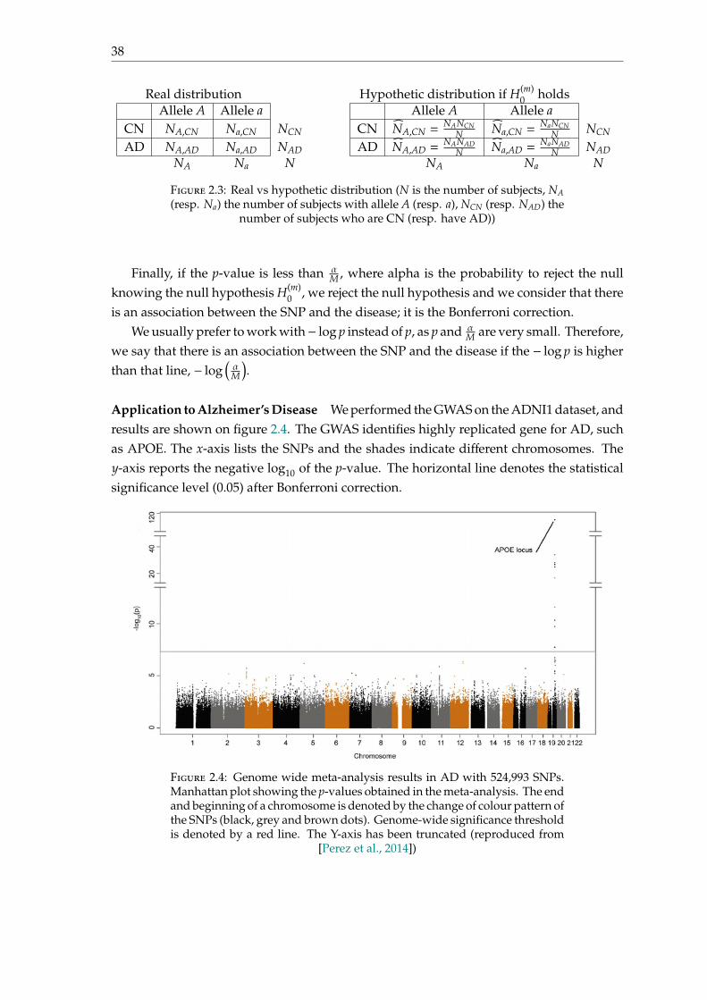
Application to Alzheimer’s Disease We performed the GWAS on the ADNI1 dataset, andresults are shown on figure 2.4. The GWAS identifies highly replicated gene for AD, suchas APOE. The x-axis lists the SNPs and the shades indicate different chromosomes. They-axis reports the negative log10 of the p-value. The horizontal line denotes the statisticalsignificance level (0.05) after Bonferroni correction.

Figure 2.4: Genome wide meta-analysis results in AD with 524,993 SNPs.Manhattan plot showing the p-values obtained in the meta-analysis. The endand beginning of a chromosome is denoted by the change of colour pattern ofthe SNPs (black, grey and brown dots). Genome-wide significance thresholdis denoted by a red line. The Y-axis has been truncated (reproduced from

[Perez et al., 2014])

2.2. Univariate and multivariate analyses between genetic and neuroimaging data 39

2.2.2 Multivariate analyses

Multivariate analyses are more appropriate when we want to explain several biomarkersby a combinaison of SNPs. There are modelling that only built the association matrix thegenetic SNPs, and the neuroimaging features such as the Partial Least Squares (PLS); andother modelling, that compute a linear regression of the biomarkers as a function of geneticdata:

biomarker ≈∑

i

αiSNPi

Theses modelling are more frequent in the literature of imaging genetics; we can cite forinstance the LASSO regression between SNPs and neuroimaging data (for sparse mod-elling), Bayesian modelling or random forests on SNPs. The underlying assumption is thatthese models assume no interactions between SNPs, and that they provide independenteffects from each other.

In all cases, multivariates analyses deal with high dimensional data: the number ofsamples N is much smaller than the number of SNPs M or the number of brain regions q.

2.2.2.1 Partial Least Squares

Among methodological approaches for capturing significant genotype-phenotype interac-tions, we can cite the partial least squares (PLS) the or independent component analysis(ICA). They perform simultaneous regression and dimensionality reduction strategies.Partial least squares (PLS) is an attractive approach because it provides a parsimoniousdescription of multivariate correlation models. Furthermore, it is simple to implement[Lorenzi et al., 2016].

Let K be the number of subjects, X = (x1, . . . , xK) ∈ RN×K be the matrix of geneticSNP data and Y = (y1, . . . , yK) ∈ RM×K the matrix of neuroimaging data. Both matricesare assumed to be normalised. The goal of PLS is to build two matrices U and V thatmaximises the covariance between XU and XV:

max∥U∥=∥V∥=1

cov(XU,YV)

Using the singular value decomposition (SVD), the previous formulation is equivalentto find unitary matrices U and V such that

XY⊤ = UΛV with U ∈ UM(R),V ∈ UK(R)

The built mapping (x,y) 7→ (x⊤U,y⊤V) provides the low dimensional representationon the latent PLS space.

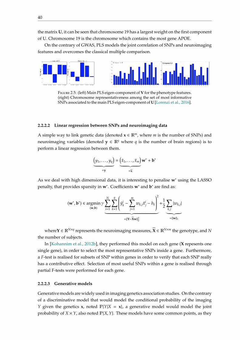
The authors have tested on the ADNI1 and ADNI2 datasets. Figure 2.5 shows themain PLS eigen-component for V (on the left) for the phenotype feature, and on the right,the main PLS eigen-component for U are shown. In the first component of V, ventriclesvolume is anti-correlated wrt the volume of the other brain areas, whereas on the secondcomponent, the hippocampal volume is anti-correlated wrt the other brain structures. In

40

the matrix U, it can be seen that chromosome 19 has a largest weight on the first componentof U. Chromosome 19 is the chromosome which contains the most gene APOE.

On the contrary of GWAS, PLS models the joint correlation of SNPs and neuroimagingfeatures and overcomes the classical multiple comparison.

Figure 2.5: (left) Main PLS eigen-component of V for the phenotype features.(right) Chromosome representativeness among the set of most informativeSNPs associated to the main PLS eigen-component of U [Lorenzi et al., 2016].

2.2.2.2 Linear regression between SNPs and neuroimaging data

A simple way to link genetic data (denoted x ∈ Rm, where m is the number of SNPs) andneuroimaging variables (denoted y ∈ Rq where q is the number of brain regions) is toperform a linear regression between them.(

y1, . . . , yq

)︸ ︷︷ ︸

=y

=(x1, . . . , xm

)︸ ︷︷ ︸

=x

w∗ + b∗

As we deal with high dimensional data, it is interesting to penalise w∗ using the LASSOpenalty, that provides sparsity in w∗. Coefficients w∗ and b∗ are find as:

(w∗,b∗) ∈ argmin(w,b)

γN∑

i=1

q∑k=1

yik −

m∑j=1

wk, jxij − bk

2

︸ ︷︷ ︸=∥Y−Xw∥22

+12

∑k, j

|wk, j|︸ ︷︷ ︸=∥w∥1

whereY ∈ RN×q represents the neuroimaging measures, X ∈ RN×m the genotype, and Nthe number of subjects.

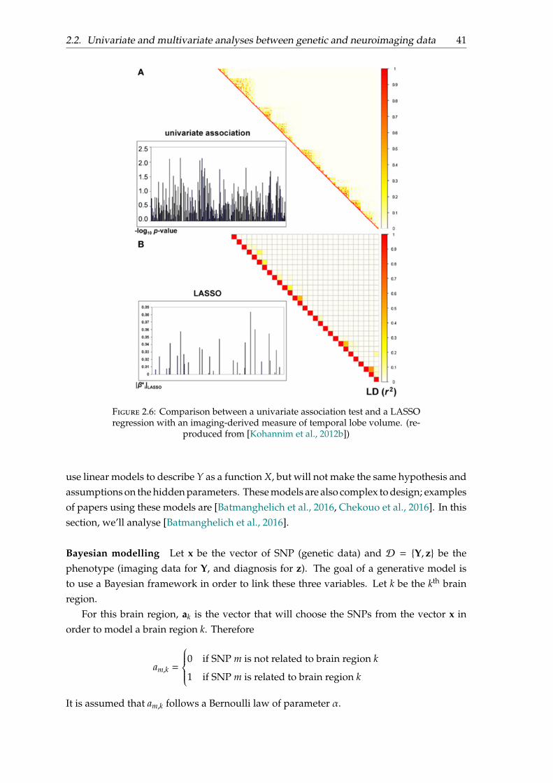
In [Kohannim et al., 2012b], they performed this model on each gene (X repesents onesingle gene), in order to select the most representative SNPs inside a gene. Furthermore,a F-test is realised for subsets of SNP within genes in order to verify that each SNP reallyhas a contributive effect. Selection of most useful SNPs within a gene is realised throughpartial F-tests were performed for each gene.

2.2.2.3 Generative models

Generative models are widely used in imaging genetics association studies. On the contraryof a discriminative model that would model the conditional probability of the imagingY given the genetics x, noted PY|X = x, a generative model would model the jointprobability of X × Y, also noted PX,Y. These models have some common points, as they

2.2. Univariate and multivariate analyses between genetic and neuroimaging data 41

Figure 2.6: Comparison between a univariate association test and a LASSOregression with an imaging-derived measure of temporal lobe volume. (re-

produced from [Kohannim et al., 2012b])

use linear models to describe Y as a function X, but will not make the same hypothesis andassumptions on the hidden parameters. These models are also complex to design; examplesof papers using these models are [Batmanghelich et al., 2016, Chekouo et al., 2016]. In thissection, we’ll analyse [Batmanghelich et al., 2016].

Bayesian modelling Let x be the vector of SNP (genetic data) and D = Y, z be thephenotype (imaging data for Y, and diagnosis for z). The goal of a generative model isto use a Bayesian framework in order to link these three variables. Let k be the kth brainregion.

For this brain region, ak is the vector that will choose the SNPs from the vector x inorder to model a brain region k. Therefore

am,k =

0 if SNP m is not related to brain region k

1 if SNP m is related to brain region k

It is assumed that am,k follows a Bernoulli law of parameter α.

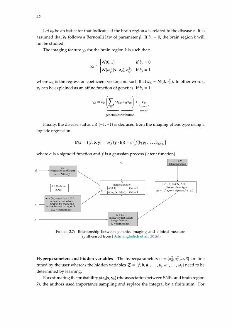
42

Let bk be an indicator that indicates if the brain region k is related to the disease z. It isassumed that bk follows a Bernoulli law of parameter β. If bk = 0, the brain region k willnot be studied.

The imaging feature yk for the brain region k is such that:

yk ∼

N(0, 1) if bk = 0

N(ω⊤k (x · ak), σ20) if bk = 1

where ωk is the regression coefficient vector, and such that ωk ∼ N(0, σ2ω). In other words,

yk can be explained as an affine function of genetics. If bk = 1:

yk ≈ bk

∑mωk,mamxm

︸ ︷︷ ︸genetics contribution

+ εk︸︷︷︸noise

Finally, the disease status z ∈ −1,+1 is deduced from the imaging phenotype using alogistic regression:

Pz = 1| f ,b,y = σ( f (y · b)) = σ(

f (b1y1, . . . , bqyq))

where σ is a sigmoid function and f is a gaussian process (latent function).

α

x = (xm)m SNP

(SNP)

ak = (am,k)m SNP, am,k ∈ 0, 1indicator that selects

image feature in region kSNP m for modeling

am,k = Bernoulli(α)

σ2ω

ωkregression coefficient

ωk ∼ N(0, σ2ω)

yk

image feature k

yk ∼N(0, 1) if bk = 0N(ω⊤k (x · ak), σ2

0) if bk = 1

σ20

β

bk ∈ 0, 1indicator that selects

image feature kbk = Bernoulli(β)

z ∈ −1, 1 (CN, AD)

p(z = 1| f ,b,y) = sigmoid( f (y · b))disease phenotype

f ∼ GPlatent function

Figure 2.7: Relationship between genetic, imaging and clinical measure(synthesised from [Batmanghelich et al., 2016])

Hyperparameters and hidden variables The hyperparameters π = σ20, σ

2ω, α, β are fine

tuned by the user whereas the hidden variablesZ = f ,b, a1, . . . , aq, ω1, . . . , ωq need to bedetermined by learning.

For estimating the probability p(ak|x,yk) (the association between SNPs and brain regionk), the authors used importance sampling and replace the integral by a finite sum. For

2.2. Univariate and multivariate analyses between genetic and neuroimaging data 43

i ∈ 1, . . . , L, they set π′(i) =(log10 α(i), σ2

0(i), σ2ω(i)

). Then,

p(am,k = 1|x,yk) =∫

p(am,k = 1|x,yk, π′)p(π′|x,yk)dπ′

=

∑Li=1 p(am,k = 1|x,yk, π

′(i))ζ(π′(i))∑Li=1 ζ(π′(i))

where ζ(π) ∝ p(π|x,yk) p(π)p(π) and p(·) is the proposal distribution, in that case, they chose

the uniform distribution. For computing p(am,k = 1|x,yk, π′(i)), they use the EM algorithm.

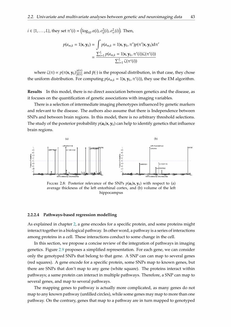
Results In this model, there is no direct association between genetics and the disease, asit focuses on the quantification of genetic associations with imaging variables.

There is a selection of intermediate imaging phenotypes influenced by genetic markersand relevant to the disease. The authors also assume that there is Independence betweenSNPs and between brain regions. In this model, there is no arbitrary threshold selections.The study of the posterior probability p(ak|x,yk) can help to identify genetics that influencebrain regions.

Figure 2.8: Posterior relevance of the SNPs p(ak|x,yk) with respect to (a)average thickness of the left entorhinal cortex, and (b) volume of the left

hippocampus

2.2.2.4 Pathways-based regression modelling

As explained in chapter 2, a gene encodes for a specific protein, and some proteins mightinteract together in a biological pathway. In other word, a pathway is a series of interactionsamong proteins in a cell. These interactions conduct to some change in the cell.

In this section, we propose a concise review of the integration of pathways in imaginggenetics. Figure 2.9 proposes a simplified representation. For each gene, we can consideronly the genotyped SNPs that belong to that gene. A SNP can can map to several genes(red squares). A gene encode for a specific protein, some SNPs map to known genes, butthere are SNPs that don’t map to any gene (white square). The proteins interact withinpathways; a same protein can interact in multiple pathways. Therefore, a SNP can map toseveral genes, and map to several pathways.

The mapping genes to pathway is actually more complicated, as many genes do notmap to any known pathway (unfilled circles), while some genes may map to more than onepathway. On the contrary, genes that map to a pathway are in turn mapped to genotyped

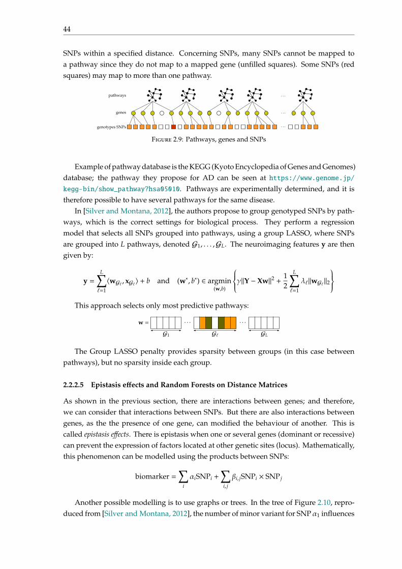
44

SNPs within a specified distance. Concerning SNPs, many SNPs cannot be mapped toa pathway since they do not map to a mapped gene (unfilled squares). Some SNPs (redsquares) may map to more than one pathway.

pathways

genes

genotypes SNPs

. . .

. . .

. . .

Figure 2.9: Pathways, genes and SNPs

Example of pathway database is the KEGG (Kyoto Encyclopedia of Genes and Genomes)database; the pathway they propose for AD can be seen at https://www.genome.jp/kegg-bin/show_pathway?hsa05010. Pathways are experimentally determined, and it istherefore possible to have several pathways for the same disease.

In [Silver and Montana, 2012], the authors propose to group genotyped SNPs by path-ways, which is the correct settings for biological process. They perform a regressionmodel that selects all SNPs grouped into pathways, using a group LASSO, where SNPsare grouped into L pathways, denoted G1, . . . ,GL. The neuroimaging features y are thengiven by:

y =L∑ℓ=1

⟨wGℓ , xGℓ⟩ + b and (w∗, b∗) ∈ argmin(w,b)

γ∥Y − Xw∥2 + 12

L∑ℓ=1

λℓ∥wGℓ∥2

This approach selects only most predictive pathways:

. . .. . .

G1 Gℓ GL

w =

The Group LASSO penalty provides sparsity between groups (in this case betweenpathways), but no sparsity inside each group.

2.2.2.5 Epistasis effects and Random Forests on Distance Matrices

As shown in the previous section, there are interactions between genes; and therefore,we can consider that interactions between SNPs. But there are also interactions betweengenes, as the the presence of one gene, can modified the behaviour of another. This iscalled epistasis effects. There is epistasis when one or several genes (dominant or recessive)can prevent the expression of factors located at other genetic sites (locus). Mathematically,this phenomenon can be modelled using the products between SNPs:

biomarker =∑

i

αiSNPi +∑

i, j

βi, jSNPi × SNP j

Another possible modelling is to use graphs or trees. In the tree of Figure 2.10, repro-duced from [Silver and Montana, 2012], the number of minor variant for SNP α1 influences

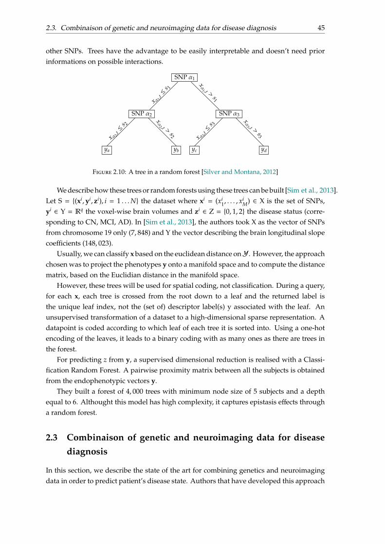
2.3. Combinaison of genetic and neuroimaging data for disease diagnosis 45

other SNPs. Trees have the advantage to be easily interpretable and doesn’t need priorinformations on possible interactions.

SNP α1

x α 1,t≤ s 1

xα1 ,t >

s1

SNP α3

x α 3,t≤ s 3

xα3 ,t >

s3

SNP α2x α 2,

t≤ s 2

xα2 ,t >

s2

ya yb yc yd

Figure 2.10: A tree in a random forest [Silver and Montana, 2012]

We describe how these trees or random forests using these trees can be built [Sim et al., 2013].Let S = (xi,yi, zi), i = 1 . . .N the dataset where xi = (xi

1, . . . , xiM) ∈ X is the set of SNPs,

yi ∈ Y = Rq the voxel-wise brain volumes and zi ∈ Z = 0, 1, 2 the disease status (corre-sponding to CN, MCI, AD). In [Sim et al., 2013], the authors took X as the vector of SNPsfrom chromosome 19 only (7, 848) and Y the vector describing the brain longitudinal slopecoefficients (148, 023).

Usually, we can classify x based on the euclidean distance onY. However, the approachchosen was to project the phenotypes y onto a manifold space and to compute the distancematrix, based on the Euclidian distance in the manifold space.

However, these trees will be used for spatial coding, not classification. During a query,for each x, each tree is crossed from the root down to a leaf and the returned label isthe unique leaf index, not the (set of) descriptor label(s) y associated with the leaf. Anunsupervised transformation of a dataset to a high-dimensional sparse representation. Adatapoint is coded according to which leaf of each tree it is sorted into. Using a one-hotencoding of the leaves, it leads to a binary coding with as many ones as there are trees inthe forest.

For predicting z from y, a supervised dimensional reduction is realised with a Classi-fication Random Forest. A pairwise proximity matrix between all the subjects is obtainedfrom the endophenotypic vectors y.

They built a forest of 4, 000 trees with minimum node size of 5 subjects and a depthequal to 6. Althought this model has high complexity, it captures epistasis effects througha random forest.

2.3 Combinaison of genetic and neuroimaging data for diseasediagnosis

In this section, we describe the state of the art for combining genetics and neuroimagingdata in order to predict patient’s disease state. Authors that have developed this approach

46

consider that genetics and neuroimaging data provide different type of information con-cerning the patient’s disease state, but that they are complementary and that genetics datacan refine the diagnosis given by neuroimaging data.

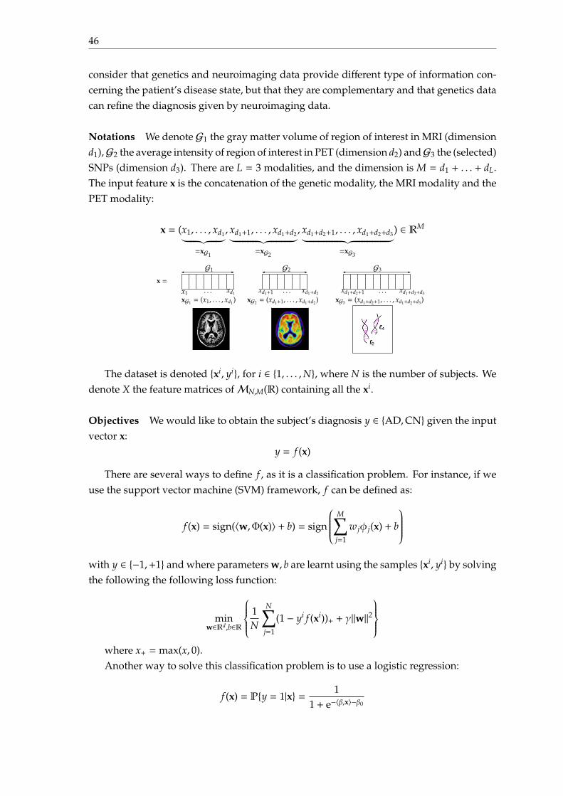
Notations We denote G1 the gray matter volume of region of interest in MRI (dimensiond1),G2 the average intensity of region of interest in PET (dimension d2) andG3 the (selected)SNPs (dimension d3). There are L = 3 modalities, and the dimension is M = d1 + . . . + dL.The input feature x is the concatenation of the genetic modality, the MRI modality and thePET modality:

x = (x1, . . . , xd1︸ ︷︷ ︸=xG1

, xd1+1, . . . , xd1+d2︸ ︷︷ ︸=xG2

, xd1+d2+1, . . . , xd1+d2+d3︸ ︷︷ ︸=xG3

) ∈ RM

x =

G3G2G1

x1 xd1 xd1+1 xd1+d2+1xd1+d2 xd1+d2+d3

xG1 = (x1, . . . , xd1) xG2 = (xd1+1, . . . , xd1+d2) xG3 = (xd1+d2+1, . . . , xd1+d2+d3). . . . . .. . .

The dataset is denoted xi, yi, for i ∈ 1, . . . ,N, where N is the number of subjects. Wedenote X the feature matrices ofMN,M(R) containing all the xi.

Objectives We would like to obtain the subject’s diagnosis y ∈ AD,CN given the inputvector x:

y = f (x)

There are several ways to define f , as it is a classification problem. For instance, if weuse the support vector machine (SVM) framework, f can be defined as:

f (x) = sign(⟨w,Φ(x)⟩ + b) = sign

M∑j=1

w jϕ j(x) + b

with y ∈ −1,+1 and where parameters w, b are learnt using the samples xi, yi by solvingthe following the following loss function:

minw∈Rd,b∈R

1N

N∑j=1

(1 − yi f (xi))+ + γ∥w∥2

where x+ = max(x, 0).Another way to solve this classification problem is to use a logistic regression:

f (x) = Py = 1|x = 11 + e−⟨β,x⟩−β0

2.3. Combinaison of genetic and neuroimaging data for disease diagnosis 47

with y ∈ 0,+1. The parameters β, β0 are determined by minimizing the loss function:

J(β, β0) =1N

N∑i=1

(−yi log f (xi) + (1 − yi) log(1 − f (xi))

)2.3.1 Dealing with high dimensional data

The high dimensional hypothesis signifies M≫ N. The gram matrix X⊤X is an element ofMM(R), but its rank is lower than N ≪ M. In this case, this matrix is not invertible andill-conditionned. It is therefore not possible to solve the previous problem. The standardimprovement is to minimise the loss with an additional penalty:

minf∈F

1N

N∑i=1

L( f (xi),yi)︸ ︷︷ ︸empirical risk

+γ Ω( f )︸︷︷︸penalty

where L is the loss function (it depends on the definition of f ), Ω is a penalty that willimpose regularisation on the function f , and γ > 0. The penalised problem must be convexw.r.t. the coefficients of the function f , and therefore can be easily solved.

We illustrate different possible penalties, using the logistic regression model.

Ridge regression The ridge penalty is defined byΩ(β) = ∥β∥22. It adds squared magnitudeof coefficients to the loss function. When γ = 0, we get the ordinary minimization problem.When γ becomes large, the penalty will add too much weight to the loss function, and willlead to under-fitting. The ridge penalty usually imposes some kind of regularity in thecoefficients of β. The choice of γ is crucial to avoid under-fitting and overfitting issue.

LASSO regression (Least Absolute Shrinkage and Selection Operator) The LASSOpenalty is defined by Ω(β) = ∥β∥1. It adds absolute magnitude of coefficients to the lossfunction. The difference between the ridge and the LASSO regression, is that the LASSOforces less important features’ coefficients to 0, and therefore it removes some featuresfrom the model. The larger γ is, the more features will be removed from the model. If γis too big, no features will be selected in the model. In other words, the LASSO regressionprovides sparsity between features.

Group LASSO regression LetG1, . . . ,GL be L groups such thatGi∩G j = ∅ andG1∪ . . .∪GL = 1, . . . ,M. The Group LASSO penalty [Ming and Yi, 2006] is defined by:

Ω(β) =L∑ℓ=1

αℓ∥βGℓ∥2

where βGℓ is the vector of β where indices Gℓ are chosen, and αℓ > 0 is the weight of thegroup ℓ (usually, αℓ =

√|Gℓ|).

The Group LASSO provides sparsity between groups, and not between variables.

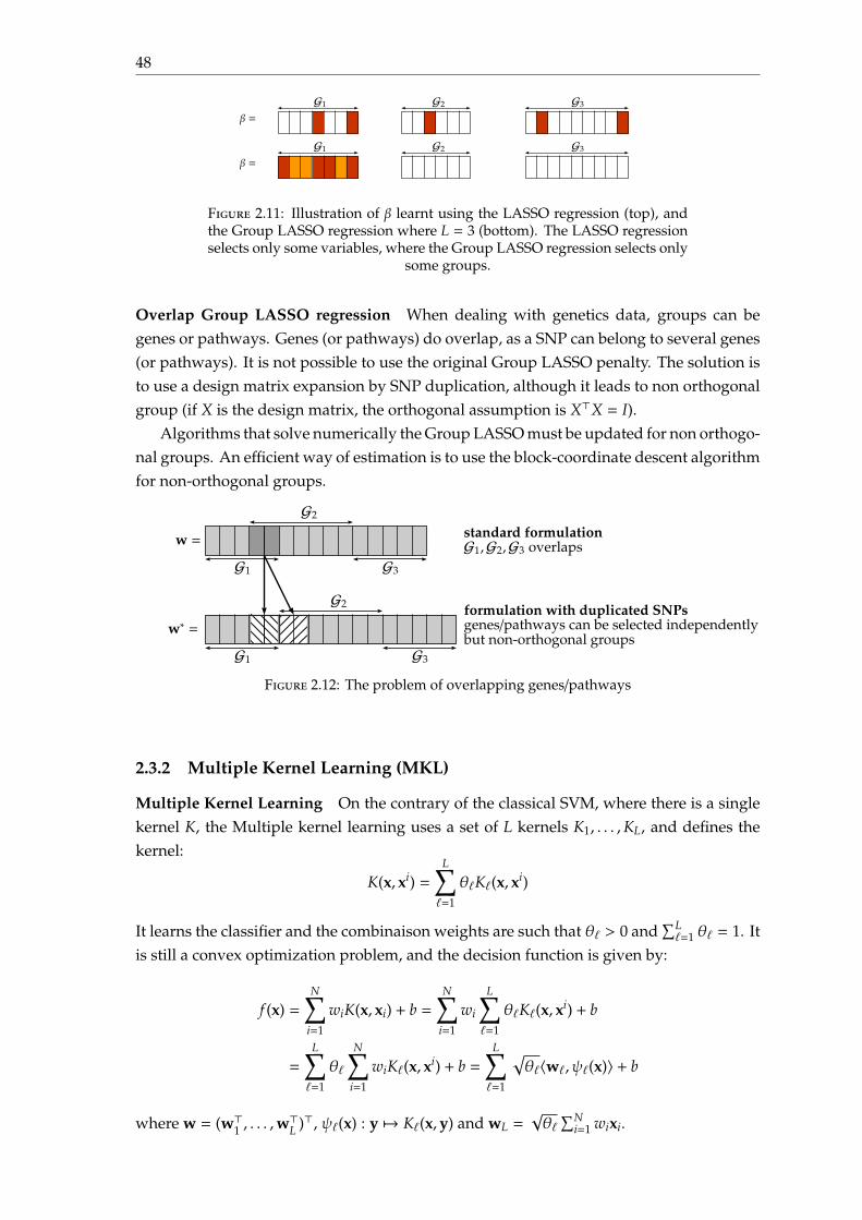
48

β =

G3G2G1

β =

G3G2G1

Figure 2.11: Illustration of β learnt using the LASSO regression (top), andthe Group LASSO regression where L = 3 (bottom). The LASSO regressionselects only some variables, where the Group LASSO regression selects only

some groups.

Overlap Group LASSO regression When dealing with genetics data, groups can begenes or pathways. Genes (or pathways) do overlap, as a SNP can belong to several genes(or pathways). It is not possible to use the original Group LASSO penalty. The solution isto use a design matrix expansion by SNP duplication, although it leads to non orthogonalgroup (if X is the design matrix, the orthogonal assumption is X⊤X = I).

Algorithms that solve numerically the Group LASSO must be updated for non orthogo-nal groups. An efficient way of estimation is to use the block-coordinate descent algorithmfor non-orthogonal groups.

w =

G1 G3

G2

G1 G3

G2

w∗ =

standard formulationG1,G2,G3 overlaps

formulation with duplicated SNPsgenes/pathways can be selected independentlybut non-orthogonal groups

Figure 2.12: The problem of overlapping genes/pathways

2.3.2 Multiple Kernel Learning (MKL)

Multiple Kernel Learning On the contrary of the classical SVM, where there is a singlekernel K, the Multiple kernel learning uses a set of L kernels K1, . . . ,KL, and defines thekernel:

K(x, xi) =L∑ℓ=1

θℓKℓ(x, xi)

It learns the classifier and the combinaison weights are such that θℓ > 0 and∑Lℓ=1 θℓ = 1. It

is still a convex optimization problem, and the decision function is given by:

f (x) =N∑

i=1

wiK(x, xi) + b =N∑

i=1

wi

L∑ℓ=1

θℓKℓ(x, xi) + b

=

L∑ℓ=1

θℓ

N∑i=1

wiKℓ(x, xi) + b =L∑ℓ=1

√θℓ⟨wℓ, ψℓ(x)⟩ + b

where w = (w⊤1 , . . . ,w⊤L )⊤, ψℓ(x) : y 7→ Kℓ(x,y) and wL =

√θℓ

∑Ni=1 wixi.

2.3. Combinaison of genetic and neuroimaging data for disease diagnosis 49

All the parameters wi, θℓ, b are learnt together. The multiple kernel learning can effi-ciently concatenate different modalities.

minw∈Rd,b∈R,θ≥0

1N

N∑j=1

L( f (xi), yi) + γ12

L∑ℓ=1

∥wℓ∥2 + γ′Ω(θ)

Equivalently, this problem is similar to, with wm ← θmwm:

minw∈Rd,b∈R,θ≥0

1N

N∑j=1

L L∑ℓ=1

⟨wℓ, ψℓ(xi)⟩ + b, yi

+ γ12

L∑ℓ=1

∥wℓ∥2θm

+ γ′Ω(θ)

There are several possible penalties, such asΩ(θ) = ∥θ∥1 that will enforce sparse kernel

mixtures; or Ω(θ) = ∥θ∥2 for non-sparse solution.

ℓp-norm MKL In the ℓp-MKL, we set Ω(θ) = ∥θ∥p =(∑M

m=1 θpm

) 1p .

Application of ℓp-norm MKL to Alzheimer’s Disease In [Peng et al., 2016], the authorspropose to set one linear kernel per feature and they want to learn the weights for eachcoefficient using a regulation ℓ1,p. The advantage of that norm is that it provides sparsityinside groups but also understand that some features can be grouped together. Theregularisation is particular; the ℓ1 norm exploits the data structure while the ℓ1,2 normprovides sparsity between features.

They start by defining one kernel per modality:

K =L∑ℓ=1

∑m∈Gℓ

θmKm with Km(x, x′) = xmx′m

Then, their decision function is given by:

f (x) =L∑ℓ=1

∑m∈Gℓ

√θmw⊤mxm + b

where the parameters w, b and θ are determined through the following minimizationproblem:

minθ

minwm,b

γN∑

i=1

L( f (xi), yi) +12

L∑ℓ=1

∑m∈Gℓ

∥wm∥22θm

with ∥θ∥1,p ≤ τ and 0 ≤ θ

The loss used is L(t, y) = (1 − yt)+. The ∥.∥1,p norm is defined by:

∥θ∥1,p = L∑ℓ=1

γℓ

∑m∈Gℓ

βm|θm|

p1p

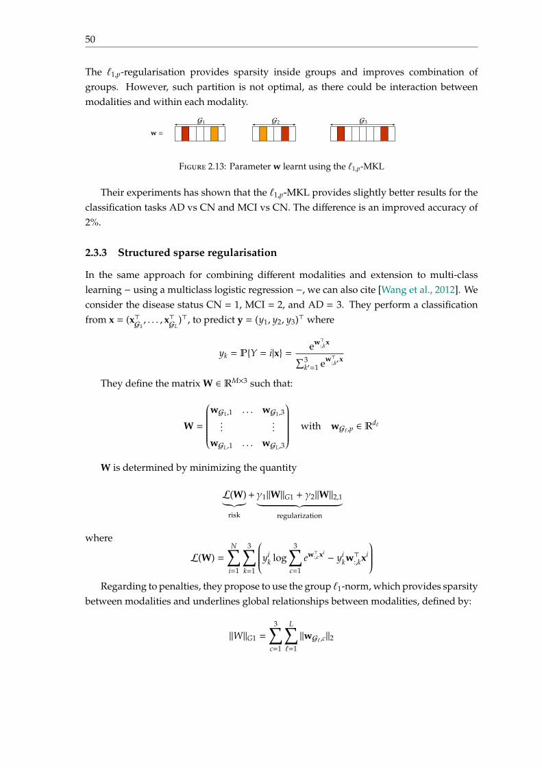
50

The ℓ1,p-regularisation provides sparsity inside groups and improves combination ofgroups. However, such partition is not optimal, as there could be interaction betweenmodalities and within each modality.

w =

G3G2G1

Figure 2.13: Parameter w learnt using the ℓ1,p-MKL

Their experiments has shown that the ℓ1,p-MKL provides slightly better results for theclassification tasks AD vs CN and MCI vs CN. The difference is an improved accuracy of2%.

2.3.3 Structured sparse regularisation

In the same approach for combining different modalities and extension to multi-classlearning − using a multiclass logistic regression −, we can also cite [Wang et al., 2012]. Weconsider the disease status CN = 1, MCI = 2, and AD = 3. They perform a classificationfrom x = (x⊤G1

, . . . , x⊤GL)⊤, to predict y = (y1, y2, y3)⊤ where

yk = PY = i|x = ew⊤:,kx∑3k′=1 ew⊤

:,k′x

They define the matrix W ∈ RM×3 such that:

W =

wG1,1 . . . wG1,3...

...

wGL,1 . . . wGL,3

with wGℓ,p ∈ Rdℓ

W is determined by minimizing the quantity

L(W)︸︷︷︸risk

+γ1∥W∥G1 + γ2∥W∥2,1︸ ︷︷ ︸regularization

where

L(W) =N∑

i=1

3∑k=1

yik log

3∑c=1

ew⊤:,cxi − yikw⊤:,kxi

Regarding to penalties, they propose to use the group ℓ1-norm, which provides sparsity

between modalities and underlines global relationships between modalities, defined by:

∥W∥G1 =

3∑c=1

L∑ℓ=1

∥wGℓ,c∥2

2.4. Conclusion 51

They also propose to use the ℓ2,1-norm which emphasises sparsity between all features andnon-sparsity between tasks, defined by:

∥W∥2,1 =M∑

m=1

∥wm,:∥2 where wm,: =(wm,1 wm,2 wm,3

)The authors of [Wang et al., 2012] have applied their model to data from ADNI, and

using the genetic (SNPs), and neuroimaging (MRI and PET scans) modalities. They con-cluded that their model provided better performances overall, with an average accuracyof 72.6 ± 3.2 %; while the MKL method with ℓ∞ penalty has an average accuracy of 62.4 ±3.1%.

2.4 Conclusion

This chapter provides a review of statistical and machine learning approaches for imaginggenetics. One of the research area is to consider that genetics can explain neuroimagingdata, but does not relate it with the disease status.

Another research area is to consider that genetics and neuroimaging data capturedifferent but complementary features. The state of the art in this area usually focuseson using linear (or pseudo-linear) models with adapted penalties. Penalties are chosen inorder to optimise the weight of each modality in the decision function, but also the optimisethe weight of each coefficients within each modality. These penalties are compulsory, aswe work with high dimensional data, and help to highlight features that are related tothe disease. The question raised from this approach is: Are linear models adapted for thecombinaison of modalities from different sources?

It is possible to apply these models to the more interesting classification tasks pMCI(progressive MCI at date T) vs sMCI (stable MCI at date T), with T that could be changed,in order to deduce at the end if the MCI patient has converted to AD, and if yes, whenhe has converted to AD. In the classification framework, this task will require to rundifferent classifiers for different T ∈ 6, 12, 18, 24, 30, 36, 42, 48, . . .. Furthermore, the pathto conversion, using the classification framework, does not ensure that it is monotonous.In the next chapter, we will focus on other approaches for predicting the conversion datefrom MCI patients.

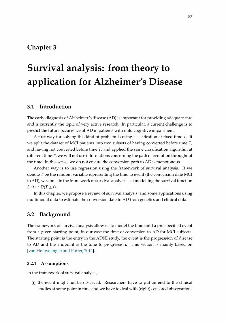
53

Chapter 3

Survival analysis: from theory toapplication for Alzheimer’s Disease

3.1 Introduction

The early diagnosis of Alzheimer’s disease (AD) is important for providing adequate careand is currently the topic of very active research. In particular, a current challenge is topredict the future occurrence of AD in patients with mild cognitive impairment.

A first way for solving this kind of problem is using classification at fixed time T. Ifwe split the dataset of MCI patients into two subsets of having converted before time T,and having not converted before time T; and applied the same classification algorithm atdifferent time T, we will not use informations concerning the path of evolution throughoutthe time. In this sense, we do not ensure the conversion path to AD is monotonous.

Another way is to use regression using the framework of survival analysis. If wedenote T be the random variable representing the time to event (the conversion date MCIto AD), we aim− in the framework of survival analysis− at modelling the survival functionS : t 7→ P(T ≥ t).

In this chapter, we propose a review of survival analysis, and some applications usingmultimodal data to estimate the conversion date to AD from genetics and clinical data.

3.2 Background

The framework of survival analysis allow us to model the time until a pre-specified eventfrom a given starting point, in our case the time of conversion to AD for MCI subjects.The starting point is the entry in the ADNI study, the event is the progression of diseaseto AD and the endpoint is the time to progression. This section is mainly based on[van Houwelingen and Putter, 2012].

3.2.1 Assumptions

In the framework of survival analysis,

(i) the event might not be observed. Researchers have to put an end to the clinicalstudies at some point in time and we have to deal with (right) censored observations

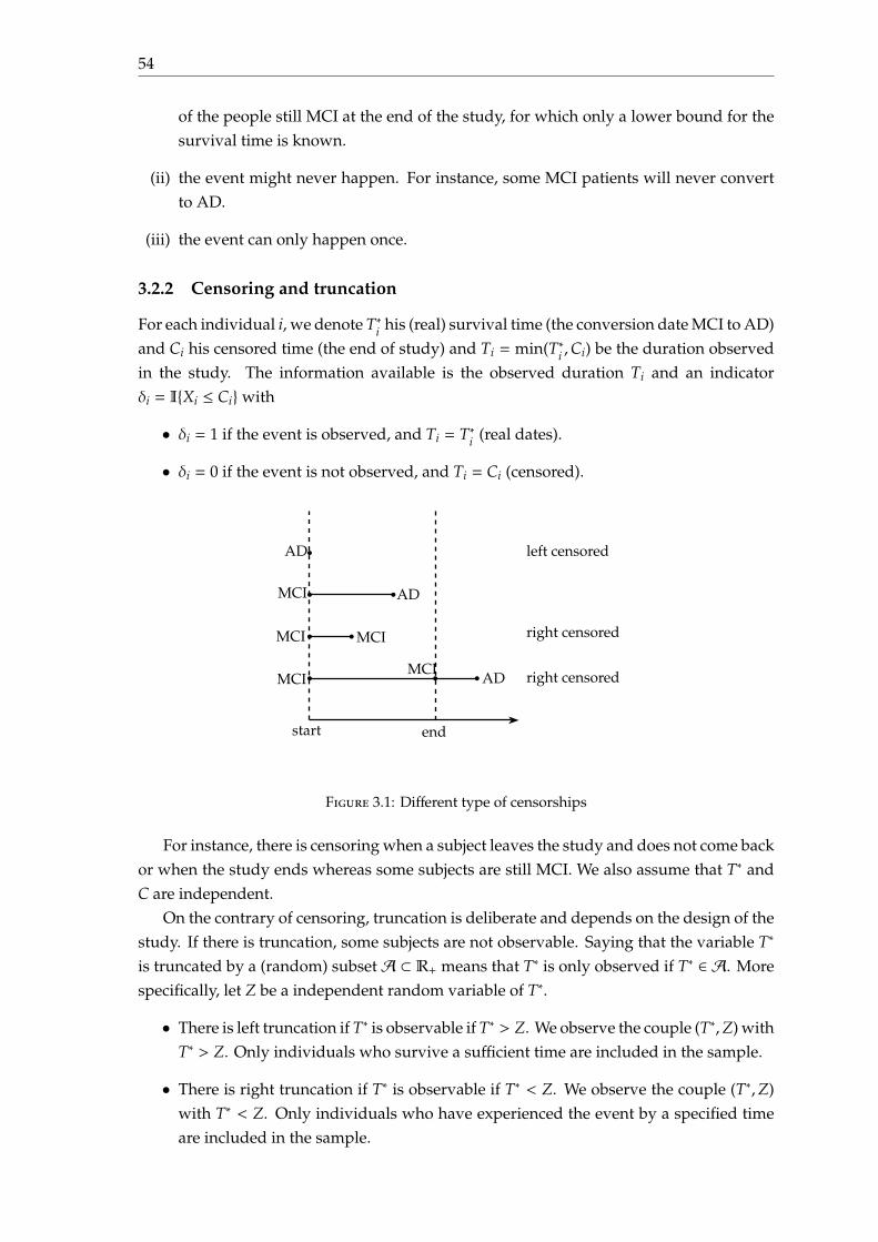
54

of the people still MCI at the end of the study, for which only a lower bound for thesurvival time is known.

(ii) the event might never happen. For instance, some MCI patients will never convertto AD.

(iii) the event can only happen once.

3.2.2 Censoring and truncation

For each individual i, we denote T∗i his (real) survival time (the conversion date MCI to AD)and Ci his censored time (the end of study) and Ti = min(T∗i ,Ci) be the duration observedin the study. The information available is the observed duration Ti and an indicatorδi = IXi ≤ Ciwith

• δi = 1 if the event is observed, and Ti = T∗i (real dates).

• δi = 0 if the event is not observed, and Ti = Ci (censored).

MCI

MCI

MCI

MCI

AD

MCIAD

AD left censored

right censored

right censored

start end

b b

b b

b b b

b

Figure 3.1: Different type of censorships

For instance, there is censoring when a subject leaves the study and does not come backor when the study ends whereas some subjects are still MCI. We also assume that T∗ andC are independent.

On the contrary of censoring, truncation is deliberate and depends on the design of thestudy. If there is truncation, some subjects are not observable. Saying that the variable T∗

is truncated by a (random) subsetA ⊂ R+ means that T∗ is only observed if T∗ ∈ A. Morespecifically, let Z be a independent random variable of T∗.

• There is left truncation if T∗ is observable if T∗ > Z. We observe the couple (T∗,Z) withT∗ > Z. Only individuals who survive a sufficient time are included in the sample.

• There is right truncation if T∗ is observable if T∗ < Z. We observe the couple (T∗,Z)with T∗ < Z. Only individuals who have experienced the event by a specified timeare included in the sample.

3.2. Background 55

3.2.3 Survival and hazard function

The conversion date T is seen as a continuous random variable with probability densityfunction (p.d.f.) f , and cumulative distribution function (c.d.f.) F : t 7→ PT < t. It givesthe probability that the event has occurred before time t. However, it is convenient to workwith the complement of the cumulative distribution function, the survival function:

S(t) = PT ≥ t = 1 − F(t) =∫ ∞

tf (u)du

S is a decreasing function, S(0) = PT ≥ 0 = 1 and limt→∞ S(t) = 0.It represents the probability that the conversion has not occurred by duration t. We

also define the hazard function, or instantaneous rate of occurrence of the event, definedas

h(t) = limδt→0

Pt ≤ T < t + δt|T ≥ tδt

The hazard function is the limit when δt goes to 0 of the ratio between the conditionalprobability that the event occurs in the interval [t, t + δt[ given that it did not occur beforeand δt. The hazard function can be rewritten

h(t) = limδt→0

Pt ≤ T < t + δtδt × PT ≥ t = lim

δt→0

Pt ≤ T < t + δtδt

× 1PT ≥ t

=f (t)S(t)=−S′(t)S(t)

= − ddt

(log S(t))

Since S(0) = 1 (since the event is sure not to have occurred by duration 0), we can solvethe above expression to obtain a formula for the probability of surviving to duration t as afunction of the hazard at all durations up to t:

S(t) = exp(−

∫ t

0h(u)du

)The cumulative hazard H is defined as the sum of the risks you face going from duration

0 to t:

H(t) =∫ t

0h(u)du

A decreasing hazard function describes a phenomenon where the probability of be-coming AD in a fixed time interval in the future decreases over time. On the contrary, anincreasing hazard function describes a phenomenon where the probability of becomingAD in a fixed time interval in the future increases over time.

Median survival time The median survival time is calculated as the smallest survivaltime for which the survivor function is less than or equal to 0.5. The median survival timeis considered at the date at which the subject converts to AD.

56

3.2.4 Kaplan-Meier and Nelson-Aalen estimators

The Kaplan-Meier estimator is a non-parametric statistic used to estimate the survivalfunction from lifetime data. It mesures the fraction of patients who have converted fora certain amount of time from the baseline. Let t1, . . . , tn be the times when there isconversion to AD or censorship. At time ti, di is the number of conversions that happened,ni the number of individuals who are still MCI (have not yet converted or have beencensored) and si = ni−di the total number that haven’t failed by time ti (including censoredat ti). The Kaplan-Meier estimator is given by:

S(t) =∏

i: ti≤t

(1 − di

ni

)

From the Kaplan-Meier estimator of the survival function, the Breslow estimator of thecumulative hazard rate function can be obtained with:

H(t) = − log(S(t)) = −∑ti≤t

log(1 − di

ni

)

Another non-parametric estimator of the cumulative hazard rate function is the Nelson-Aalen estimator, given by

H(t) =∑ti≤t

di

ni

Both statistics estimate the cumulative number of expected events.

Example We consider the following dataset:

Observed Survival Time T Fail Indicator δ

1 12 0

2 24 0

3 18 1

4 6 1

5 24 1

6 30 1

7 24 0

8 24 0

9 12 1

10 12 0

We start by order the event times (6 < 12 < 18 < 24 < 30) and create the tabulate countsat each time:

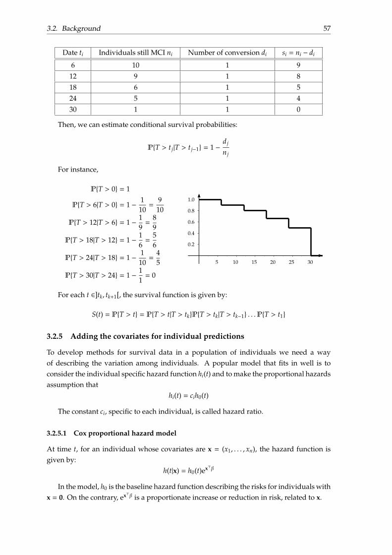
3.2. Background 57

Date ti Individuals still MCI ni Number of conversion di si = ni − di

6 10 1 9

12 9 1 8

18 6 1 5

24 5 1 4

30 1 1 0

Then, we can estimate conditional survival probabilities:

PT > t j|T > t j−1 = 1 −d j

n j

For instance,

PT > 0 = 1

PT > 6|T > 0 = 1 − 110=

910

PT > 12|T > 6 = 1 − 19=

89

PT > 18|T > 12 = 1 − 16=

56

PT > 24|T > 18 = 1 − 110=

45

PT > 30|T > 24 = 1 − 11= 0

−0.2

0.2

0.4

0.6

0.8

1.0

5 10 15 20 25 30

For each t ∈]tk, tk+1[, the survival function is given by:

S(t) = PT > t = PT > t|T > tkPT > tk|T > tk−1 . . .PT > t1

3.2.5 Adding the covariates for individual predictions

To develop methods for survival data in a population of individuals we need a wayof describing the variation among individuals. A popular model that fits in well is toconsider the individual specific hazard function hi(t) and to make the proportional hazardsassumption that

hi(t) = cih0(t)

The constant ci, specific to each individual, is called hazard ratio.

3.2.5.1 Cox proportional hazard model

At time t, for an individual whose covariates are x = (x1, . . . , xn), the hazard function isgiven by:

h(t|x) = h0(t)ex⊤β

In the model, h0 is the baseline hazard function describing the risks for individuals withx = 0. On the contrary, ex⊤β is a proportionate increase or reduction in risk, related to x.

58

This model separates the effect of time from the effect of the covariates. Taking logs,the Cox model is an additive model for the log of the hazard:

log h(t|x) = log h0(t) + x⊤β

The effect of the covariates x is the same at all times. If we integrate the hazard functionover time, we obtain H(t|x) = H0(t)ex⊤β. Then, the survival function is given by:

S(t|x) = (S0(t))ex⊤β

where S0(t) = exp(−

∫ t0 h0(u)du

)is a baseline survival function. The effect of the

covariate values x on the survivor function is to raise it to a power given by the relativerisk ex⊤β.

We also define the prognostic index as PI(x) = x⊤β.

Example We consider a two-sample problem where the x serves to identify groups one(female) and zero (male). Then the model is

h(t|x) =

h0(t) if x = 0

h0(t)eβ if x = 1

h0(t) represents the risk at time t in group 0, and eβ is the ratio of the risk in group onerelative to group zero at any time t. If eβ = 1, the risk is the same for the two groups. Onthe contrary, if eβ = 2 (or β = ln 2), then the risk for an individual in group one at any givenage is twice the risk of a member of group zero who has the same age.

3.2.5.2 Exponential model

Different forms of proportional hazard models can be obtained by making assumptionsabout the baseline survival function, or the baseline hazard function. For instance, if thebaseline risk is constant over time (h(t) = λ), then the survival function is S(t|x) = exp(−λt).λ can reparameterized in terms of predictor variables.

1

10

b

b

S

h = λ = 0.5

Figure 3.2: Survival and hazard functions for exponential model

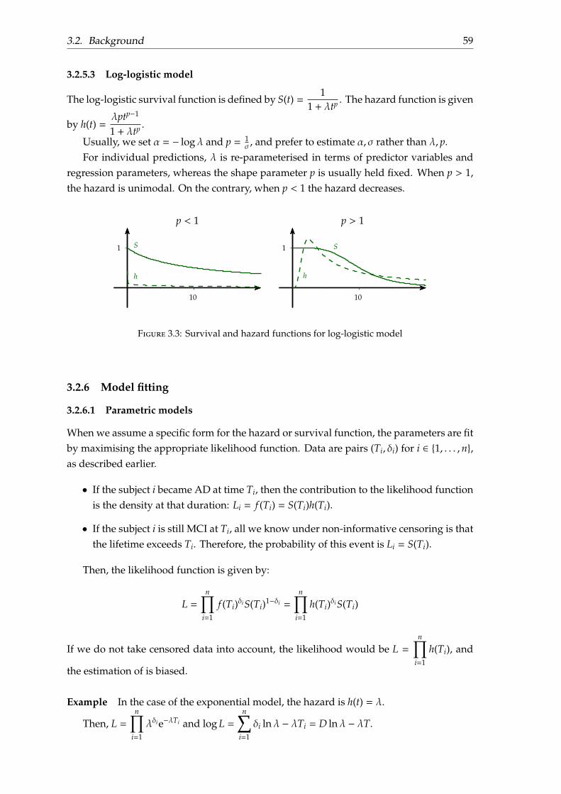
3.2. Background 59

3.2.5.3 Log-logistic model

The log-logistic survival function is defined by S(t) =1

1 + λtp . The hazard function is given

by h(t) =λptp−1

1 + λtp .

Usually, we set α = − logλ and p = 1σ , and prefer to estimate α, σ rather than λ, p.

For individual predictions, λ is re-parameterised in terms of predictor variables andregression parameters, whereas the shape parameter p is usually held fixed. When p > 1,the hazard is unimodal. On the contrary, when p < 1 the hazard decreases.

p < 1

1

10

bp = 0.9

blambda = 0.1

S

h

p > 1

1

10

bp = 3.9

blambda = 0.1

S

h

Figure 3.3: Survival and hazard functions for log-logistic model

3.2.6 Model fitting

3.2.6.1 Parametric models

When we assume a specific form for the hazard or survival function, the parameters are fitby maximising the appropriate likelihood function. Data are pairs (Ti, δi) for i ∈ 1, . . . , n,as described earlier.

• If the subject i became AD at time Ti, then the contribution to the likelihood functionis the density at that duration: Li = f (Ti) = S(Ti)h(Ti).

• If the subject i is still MCI at Ti, all we know under non-informative censoring is thatthe lifetime exceeds Ti. Therefore, the probability of this event is Li = S(Ti).

Then, the likelihood function is given by:

L =n∏

i=1

f (Ti)δiS(Ti)1−δi =

n∏i=1

h(Ti)δiS(Ti)

If we do not take censored data into account, the likelihood would be L =n∏

i=1

h(Ti), and

the estimation of is biased.

Example In the case of the exponential model, the hazard is h(t) = λ.

Then, L =n∏

i=1

λδie−λTi and log L =n∑

i=1

δi lnλ − λTi = D lnλ − λT.

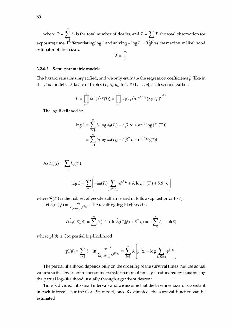
60

where D =n∑

i=1

δi is the total number of deaths, and T =n∑

i=1

Ti the total observation (or

exposure) time. Differentiating log L and solving− log L = 0 gives the maximum likelihoodestimator of the hazard:

λ =DT

3.2.6.2 Semi-parametric models

The hazard remains unspecified, and we only estimate the regression coefficients β (like inthe Cox model). Data are of triples (Ti, δi, xi) for i ∈ 1, . . . , n, as described earlier.

L =n∏

i=1

h(Ti)δiS(Ti) =n∏

i=1

h0(Ti)δieδiβ⊤xi (S0(Ti))ex⊤i β

The log-likelihood is:

log L =n∑

i=1

δi log h0(Ti) + δiβ⊤xi + ex⊤i β log (S0(Ti))

=

n∑i=1

δi log h0(Ti) + δiβ⊤xi − ex⊤i βH0(Ti)

As H0(t) =∑ti≤t

h0(Ti),

log L =n∑

i=1

−h0(Ti)∑

j∈R(Ti)

eβ⊤xi + δi log h0(Ti) + δiβ

⊤xi

where R(Ti) is the risk set of people still alive and in follow-up just prior to Ti.

Let h0(Ti|β) = δi∑j∈R(Ti)

eβ⊤xi. The resulting log-likelihood is:

ℓ(h0(·|β), β) =n∑

i=1

δi(−1 + ln h0(Ti|β) + β⊤xi) = −n∑

i=1

δi + pl(β)

where pl(β) is Cox partial log-likelihood:

pl(β) =n∑

i=1

δi · lneβ⊤xi∑

j∈R(ti) eβ⊤xi=

n∑i=1

δi

β⊤xi − log∑

j∈R(ti)

eβ⊤xi

The partial likelihood depends only on the ordering of the survival times, not the actual

values; so it is invariant to monotone transformation of time. β is estimated by maximisingthe partial log-likelihood, usually through a gradient descent.

Time is divided into small intervals and we assume that the baseline hazard is constantin each interval. For the Cox PH model, once β estimated, the survival function can beestimated

3.2. Background 61

• by the Kaplan-Meier estimator:

S(t|x) =∏Ti≤t

(1 − eβ

⊤xh0(Ti))

where h0(Ti) =δi∑

j∈R(Ti) eβ⊤xi

• or by the Nelson-Aalen estimator:

S(t|x) = exp(−H0(t)eβ

⊤x)

3.2.7 Hypotheses behind the Cox proportional hazard model

The Cox proportional hazard model h(t|x) = h0(t)eβ⊤x can fail to fit data. Some reasons can

be:

• the functional form of the covariates: instead of incorporating x j in the model, itcould be interesting to incorporate x2

j ou log(x j).

• the proportional hazard assumption is not verified: the coefficient β j is not constantin time.

• the relationship between the predictor β⊤x and the hazard is not log-linear.

We describe how the proportional hazard assumption is verified. It is equivalent to testthe null hypothesis:

H0 : β j(t) = β j

β j(t) can defined as:β j(t) = β j + θ jg j(t)

where g j is a predictable function of time. Testing H0 is equivalent to testing:

H0 : θ j = 0

We order the durations 0 ≤ T(1) ≤ . . . ≤ T(n) and x(1), . . . , x(n) the corresponding covari-ates.

At time T( j), the Schoenfeld residual for any subject i ∈ R(T( j)) is defined by:

x(i) − a( j) where a( j) =∑

ℓ∈R(T( j))

eβ⊤xℓ∑

k∈R(T( j)) eβ⊤xkxℓ

The Schoenfeld residual corresponding to T( j) is defined as the sum of the Schoenfeldresiduals over all subjects who fail at T( j):

rSh( j) =∑

i∈R(T( j))

δi j(x(i) − a( j))

where δi j = 1 if the subject i fails at T(k), 0 otherwise.The scaled Schoenfeld residual are defined by V−1

( j) rSh( j) where V( j) is the estimator of the

covariance matrix of the Schoenfeld residual rSh( j). Furthermore, E[V−1( j) rSh( j)] ≈ θ jg j(T( j)).

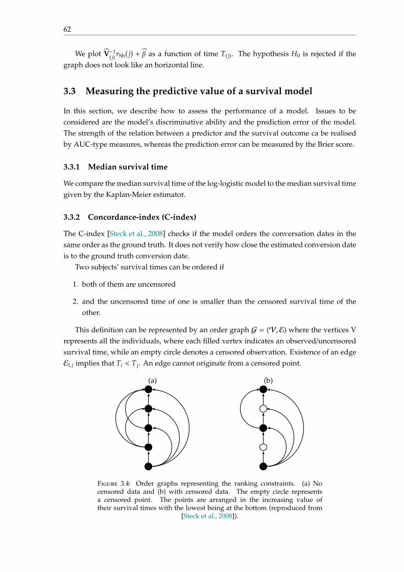
62

We plot V−1( j) rSh( j) + β as a function of time T( j). The hypothesis H0 is rejected if the

graph does not look like an horizontal line.

3.3 Measuring the predictive value of a survival model

In this section, we describe how to assess the performance of a model. Issues to beconsidered are the model’s discriminative ability and the prediction error of the model.The strength of the relation between a predictor and the survival outcome ca be realisedby AUC-type measures, whereas the prediction error can be measured by the Brier score.

3.3.1 Median survival time

We compare the median survival time of the log-logistic model to the median survival timegiven by the Kaplan-Meier estimator.

3.3.2 Concordance-index (C-index)

The C-index [Steck et al., 2008] checks if the model orders the conversation dates in thesame order as the ground truth. It does not verify how close the estimated conversion dateis to the ground truth conversion date.

Two subjects’ survival times can be ordered if

1. both of them are uncensored

2. and the uncensored time of one is smaller than the censored survival time of theother.

This definition can be represented by an order graph G = (V,E) where the vertices Vrepresents all the individuals, where each filled vertex indicates an observed/uncensoredsurvival time, while an empty circle denotes a censored observation. Existence of an edgeEi, j implies that Ti < T j. An edge cannot originate from a censored point.

(a) (b)

Figure 3.4: Order graphs representing the ranking constraints. (a) Nocensored data and (b) with censored data. The empty circle representsa censored point. The points are arranged in the increasing value oftheir survival times with the lowest being at the bottom (reproduced from

[Steck et al., 2008]).

3.3. Measuring the predictive value of a survival model 63

The C-index is the fraction of all pairs of subjects whose predicted survival times arecorrectly ordered among all subjects that can actually be ordered.

c =1|E|

∑Ei j

1 f (xi)< f (x j) =1|E|

∑Ti uncensored

∑T j>Ti

1 f (xi)< f (x j)

where |E| is the number of edges in the order graph, f (xi) is the predicted survival timefor subject i by the model f .

Therefore, the C-index does not evaluate the distance between the estimated conversiondate and the true conversion date. This measure evaluates the accuracy of the ordering ofpredicted time. As a generalisation of AUC:

• 0.5 is the expected result from random predictions,

• 1.0 is perfect concordance,

• 0.0 is perfect anti-concordance (multiply predictions with −1 to get 1.0)

For standard survival models, the C-index is between 0.6 and 0.7.

3.3.3 Cumulative AUC(t)

Let Mi be the estimated probability value for subject i, and Di(t) = 1 if Ti ≤ t et Di(t) = 0 ifTi > t. Di(t) denotes the failure (disease) status at any time t with Di(t) = 1 indicating thatsubject i has had an event prior to time t.

Sensitivity and specificity become time-dependent functions:

sensitivity(m, t) = PM > m|D(t) = 1specificity(m, t) = PM ≤ m|D(t) = 0

Each individual plays the role of a control for times t < Ti , but then contributes as acase for later times, t ≥ Ti. Using these definitions, we can define the corresponding ROCcurve for any time t, ROC(t).

If T denotes the follow-up date, and f (t) the probability density function of the time-to-event outcome related to the model, we define the integrated AUC [Chambless and Diao, 2006]by:

iAUC =∫ T

0AUC(t) × f (t)dt

As for the AUC, the range for the iAUC is in [0, 1].

3.3.4 Kullback-Leibler divergence and Brier score

If S(t0|x) denotes the model-based probabilistic prediction for the survival of an individ-ual beyond t0 given the covariates x and y = IT>t0 be the actual observation (ignoringcensoring for the time being), we define the following scores [Graf et al., 1999]:

64

KL(y, S(t0|x)) = −y log S(t0|x) − (1 − y) log(1 − S(t0|x))

Brier(y, S(t0|x)) = (y − S(t0|x))2

From these measures, a global measure can built. The time is divided into L+1 intervalsI1 = [t0 = 0, t1[, . . ., IL = [tL−1, tL[, IL+1 = [tL,+∞[, where tL is the horizon time.

The global score is then given by:

Brierglobal(t, S(t0|x)) =L+1∑ℓ=1

(It∈Iℓ − pℓ(x))2

KLglobal(t, p(x)) = −L+1∑ℓ=1

It∈Iℓ ln(pℓ(x))

where pℓ(x) = P(T ∈ Iℓ|x).These scores evaluate how well the estimated survival function fits to the ground truth.

Lower are these scores, better the model is.

3.4 Combinaison of multimodal data using the Cox PH frame-work

In this section, we describe some applications of Cox proportional hazards models usinggenetics, clinical and neuroimaging data. As for classification, the goal is to provide ananswer to the question: Can genetics data help to improve predictions and how to combinethem with clinical data?

In [van Houwelingen et al., 2006, van der Laan et al., 2007, Bøvelstad et al., 2009], theyapplied their models to the breast cancer dataset.

Notations We denote xG the vector of SNPs counted by number of minor variants, xC theclinical covariates, and T the conversion date from baseline (continuous random variable).

A first model for combining genetics and clinical data In [Bøvelstad et al., 2009], theauthors propose the following model:

h(t|xG, xC) = h0(t) exp(x⊤Gβ + x⊤Cγ)

Clinical covariates are supposed to be well-established and are all included in themodel. The high-dimensional genomic part is regularised, by adding a penalty on β suchas ℓ1 or ℓ2 penalty. According to the authors, only the ℓ2 penalty can improve predictions. Inparticular, the correlation between genetics and clinical data can lead to dramatic changesin both β and γ compared with the models with only clinical or genomic covariates.For example, adding clinical covariates can completely change the selection of genomiccovariates made by a ℓ1-regression. The implication is that the prediction model depends

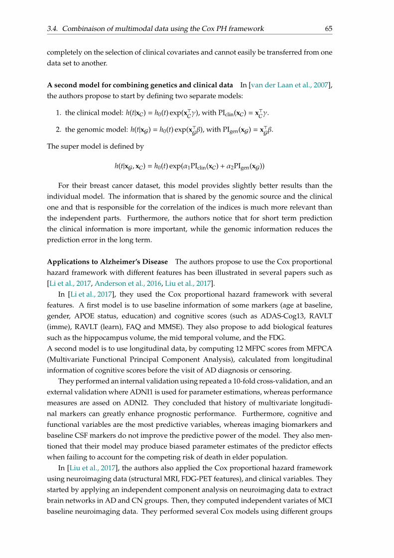
3.4. Combinaison of multimodal data using the Cox PH framework 65

completely on the selection of clinical covariates and cannot easily be transferred from onedata set to another.

A second model for combining genetics and clinical data In [van der Laan et al., 2007],the authors propose to start by defining two separate models:

1. the clinical model: h(t|xC) = h0(t) exp(x⊤Cγ), with PIclin(xC) = x⊤Cγ.

2. the genomic model: h(t|xG) = h0(t) exp(x⊤Gβ), with PIgen(xG) = x⊤Gβ.

The super model is defined by

h(t|xG, xC) = h0(t) exp(α1PIclin(xC) + α2PIgen(xG))

For their breast cancer dataset, this model provides slightly better results than theindividual model. The information that is shared by the genomic source and the clinicalone and that is responsible for the correlation of the indices is much more relevant thanthe independent parts. Furthermore, the authors notice that for short term predictionthe clinical information is more important, while the genomic information reduces theprediction error in the long term.

Applications to Alzheimer’s Disease The authors propose to use the Cox proportionalhazard framework with different features has been illustrated in several papers such as[Li et al., 2017, Anderson et al., 2016, Liu et al., 2017].

In [Li et al., 2017], they used the Cox proportional hazard framework with severalfeatures. A first model is to use baseline information of some markers (age at baseline,gender, APOE status, education) and cognitive scores (such as ADAS-Cog13, RAVLT(imme), RAVLT (learn), FAQ and MMSE). They also propose to add biological featuressuch as the hippocampus volume, the mid temporal volume, and the FDG.A second model is to use longitudinal data, by computing 12 MFPC scores from MFPCA(Multivariate Functional Principal Component Analysis), calculated from longitudinalinformation of cognitive scores before the visit of AD diagnosis or censoring.

They performed an internal validation using repeated a 10-fold cross-validation, and anexternal validation where ADNI1 is used for parameter estimations, whereas performancemeasures are assed on ADNI2. They concluded that history of multivariate longitudi-nal markers can greatly enhance prognostic performance. Furthermore, cognitive andfunctional variables are the most predictive variables, whereas imaging biomarkers andbaseline CSF markers do not improve the predictive power of the model. They also men-tioned that their model may produce biased parameter estimates of the predictor effectswhen failing to account for the competing risk of death in elder population.

In [Liu et al., 2017], the authors also applied the Cox proportional hazard frameworkusing neuroimaging data (structural MRI, FDG-PET features), and clinical variables. Theystarted by applying an independent component analysis on neuroimaging data to extractbrain networks in AD and CN groups. Then, they computed independent variates of MCIbaseline neuroimaging data. They performed several Cox models using different groups

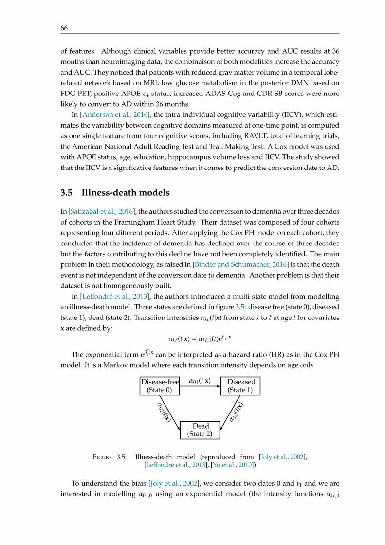
66

of features. Although clinical variables provide better accuracy and AUC results at 36months than neuroimaging data, the combinaison of both modalities increase the accuracyand AUC. They noticed that patients with reduced gray matter volume in a temporal lobe-related network based on MRI, low glucose metabolism in the posterior DMN based onFDG-PET, positive APOE ε4 status, increased ADAS-Cog and CDR-SB scores were morelikely to convert to AD within 36 months.

In [Anderson et al., 2016], the intra-individual cognitive variability (IICV), which esti-mates the variability between cognitive domains measured at one-time point, is computedas one single feature from four cognitive scores, including RAVLT, total of learning trials,the American National Adult Reading Test and Trail Making Test. A Cox model was usedwith APOE status, age, education, hippocampus volume loss and IICV. The study showedthat the IICV is a significative features when it comes to predict the conversion date to AD.

3.5 Illness-death models

In [Satizabal et al., 2016], the authors studied the conversion to dementia over three decadesof cohorts in the Framingham Heart Study. Their dataset was composed of four cohortsrepresenting four different periods. After applying the Cox PH model on each cohort, theyconcluded that the incidence of dementia has declined over the course of three decadesbut the factors contributing to this decline have not been completely identified. The mainproblem in their methodology, as raised in [Binder and Schumacher, 2016] is that the deathevent is not independent of the conversion date to dementia. Another problem is that theirdataset is not homogeneously built.

In [Leffondré et al., 2013], the authors introduced a multi-state model from modellingan illness-death model. Three states are defined in figure 3.5: disease free (state 0), diseased(state 1), dead (state 2). Transition intensities αkℓ(t|x) from state k to ℓ at age t for covariatesx are defined by:

αkℓ(t|x) = αkℓ,0(t)eβ⊤kℓx

The exponential term eβ⊤kℓx can be interpreted as a hazard ratio (HR) as in the Cox PH

model. It is a Markov model where each transition intensity depends on age only.

Disease-free Diseased(State 1)(State 0)

α01(t|x)

Dead(State 2)

α02 (t|x) α 12

(t|x)

Figure 3.5: Illness-death model (reproduced from [Joly et al., 2002],[Leffondré et al., 2013], [Yu et al., 2010])

To understand the biais [Joly et al., 2002], we consider two dates 0 and t1 and we areinterested in modelling α01,0 using an exponential model (the intensity functions αkℓ,0

3.6. Conclusion 67

are constant). In the classical two-state model, subjects who died between 0 and t1 areright-censored at 0. An estimator of the survival function at t1 is:

S(t1) =Phealthy at t1Palive at t1

Because S(t1) = e−α01,0t1 , an estimator of α01,0 is α01,0 = −1t1

log S(t1). However, in an

illness-death model,

S(t1) =Phealthy at t1Palive at t1

=1

1 + α01,0α01,0+α02,0−α12,0

(e(α01,0+α02,0−α12,0)t1 − 1)

Then,

α01,0−α01,0 = −1t1

log S(t1)+1t1

log S(t1) = − 1t1

log(α01,0e−(α12,0−α02,0)t1 − (α12,0 − α02,0)e−α01,0t1

α01,0 − (α12,0 − α02,0)

)If α12,0 = α02,0 = 0, then both models are identical.

In the general case, the estimation of αkℓ,0 [Joly et al., 2002] uses a penalised log-likelihood defined as:

pl(α01,0, α12,0, α02,0) = ℓ(α01,0, α12,0, α02,0)−λ01

∫α′′01,0(u)2du−λ12

∫α′′12,0(u)2du−λ02

∫α′′02,0(u)2du

where ℓ is the full-likelihood of the illness-death model, and λ01, λ12, λ02 are positivesmoothing parameters.

Compared with other survival models such as the Cox proportional hazard model andthe Weibull model [Leffondré et al., 2013], the illness-death model provides better estimatesof the effects on disease of the effects on disease of exposures that were associated withdeath. This model is able to account for the probability of developing the disease betweenthe last visit and death, on the contrary of classical survival model.

3.6 Conclusion

This chapter provides a review of survival analysis and its applications for disease con-version date prediction. Although survival analysis make strong assumptions concerningthe construction of the dataset (censoring and truncation) and the disease (all patientsare assumed to convert), survival analysis also provides a good regression framework fordirectly estimating the conversion date to disease. We also note that most survival modelshave underlying assumptions that are important to verify when applied to specific dataset;and that death is a competitive risk when dealing with elder population.

69

Part II

Contributions

71

Chapter 4

Multilevel Modeling with StructuredPenalties for Classification fromImaging Genetics Data

A preliminary version of this chapter has been published in the proceedings of the MICCAI2017 Workshop on Imaging Genetics.

Pascal Lu, Olivier Colliot. Multilevel Modeling with Structured Penalties forClassification from Imaging Genetics data. 3rd MICCAI Workshop on ImagingGenetics (MICGen 2017), Sep 2017, Quebec City, Canada. pp.230-240

4.1 Introduction

In this chapter, we propose a framework for automatic classification of patients frommultimodal genetic and brain imaging data by optimally combining them. Additivemodels with unadapted penalties (such as the classical group lasso penalty or ℓ1-multiplekernel learning) treat all modalities in the same manner and can result in undesirableelimination of specific modalities when their contributions are unbalanced.

To overcome this limitation, we introduce a multilevel model that combines imagingand genetics and that considers joint effects between these two modalities for diagnosisprediction. Furthermore, we propose a framework allowing to combine several penaltiestaking into account the structure of the different types of data, such as a group lasso penaltyover the genetic modality and a ℓ2-penalty on imaging modalities. Finally, we propose afast optimization algorithm, based on a proximal gradient method.

The model has been evaluated on genetic (single nucleotide polymorphisms - SNP)and imaging (anatomical MRI measures) data from the ADNI database, and compared toadditive models [Wang et al., 2012, Aiolli and Donini, 2015]. It exhibits good performancesin AD diagnosis; and at the same time, reveals relationships between genes, brain regionsand the disease status.

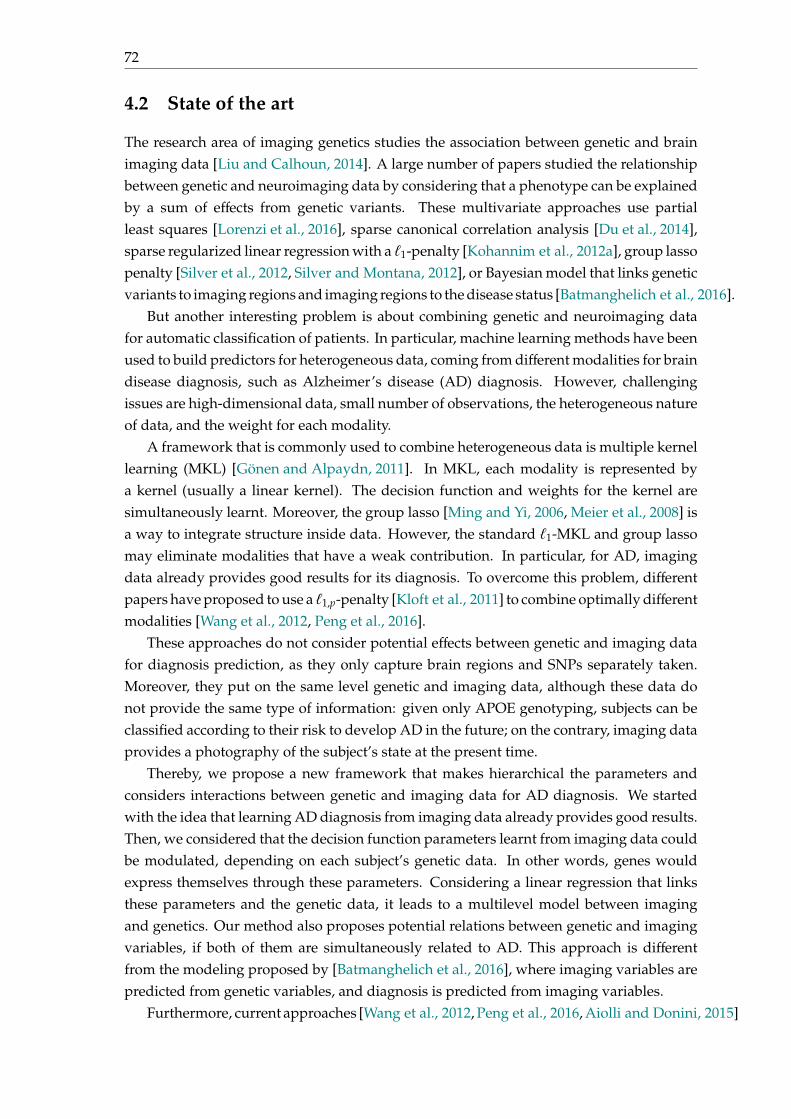
72

4.2 State of the art

The research area of imaging genetics studies the association between genetic and brainimaging data [Liu and Calhoun, 2014]. A large number of papers studied the relationshipbetween genetic and neuroimaging data by considering that a phenotype can be explainedby a sum of effects from genetic variants. These multivariate approaches use partialleast squares [Lorenzi et al., 2016], sparse canonical correlation analysis [Du et al., 2014],sparse regularized linear regression with a ℓ1-penalty [Kohannim et al., 2012a], group lassopenalty [Silver et al., 2012, Silver and Montana, 2012], or Bayesian model that links geneticvariants to imaging regions and imaging regions to the disease status [Batmanghelich et al., 2016].

But another interesting problem is about combining genetic and neuroimaging datafor automatic classification of patients. In particular, machine learning methods have beenused to build predictors for heterogeneous data, coming from different modalities for braindisease diagnosis, such as Alzheimer’s disease (AD) diagnosis. However, challengingissues are high-dimensional data, small number of observations, the heterogeneous natureof data, and the weight for each modality.

A framework that is commonly used to combine heterogeneous data is multiple kernellearning (MKL) [Gönen and Alpaydn, 2011]. In MKL, each modality is represented bya kernel (usually a linear kernel). The decision function and weights for the kernel aresimultaneously learnt. Moreover, the group lasso [Ming and Yi, 2006, Meier et al., 2008] isa way to integrate structure inside data. However, the standard ℓ1-MKL and group lassomay eliminate modalities that have a weak contribution. In particular, for AD, imagingdata already provides good results for its diagnosis. To overcome this problem, differentpapers have proposed to use a ℓ1,p-penalty [Kloft et al., 2011] to combine optimally differentmodalities [Wang et al., 2012, Peng et al., 2016].

These approaches do not consider potential effects between genetic and imaging datafor diagnosis prediction, as they only capture brain regions and SNPs separately taken.Moreover, they put on the same level genetic and imaging data, although these data donot provide the same type of information: given only APOE genotyping, subjects can beclassified according to their risk to develop AD in the future; on the contrary, imaging dataprovides a photography of the subject’s state at the present time.

Thereby, we propose a new framework that makes hierarchical the parameters andconsiders interactions between genetic and imaging data for AD diagnosis. We startedwith the idea that learning AD diagnosis from imaging data already provides good results.Then, we considered that the decision function parameters learnt from imaging data couldbe modulated, depending on each subject’s genetic data. In other words, genes wouldexpress themselves through these parameters. Considering a linear regression that linksthese parameters and the genetic data, it leads to a multilevel model between imagingand genetics. Our method also proposes potential relations between genetic and imagingvariables, if both of them are simultaneously related to AD. This approach is differentfrom the modeling proposed by [Batmanghelich et al., 2016], where imaging variables arepredicted from genetic variables, and diagnosis is predicted from imaging variables.

Furthermore, current approaches [Wang et al., 2012, Peng et al., 2016, Aiolli and Donini, 2015]

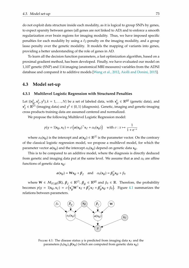
4.3. Model set-up 73

do not exploit data structure inside each modality, as it is logical to group SNPs by genes,to expect sparsity between genes (all genes are not linked to AD) and to enforce a smoothregularization over brain regions for imaging modality. Thus, we have imposed specificpenalties for each modality by using a ℓ2-penalty on the imaging modality, and a grouplasso penalty over the genetic modality. It models the mapping of variants into genes,providing a better understanding of the role of genes in AD.

To learn all the decision function parameters, a fast optimization algorithm, based on aproximal gradient method, has been developed. Finally, we have evaluated our model on1,107 genetic (SNP) and 114 imaging (anatomical MRI measures) variables from the ADNIdatabase and compared it to additive models [Wang et al., 2012, Aiolli and Donini, 2015].

4.3 Model set-up

4.3.1 Multilevel Logistic Regression with Structured Penalties

Let (xkG, x

kI, y

k), k = 1, . . . ,N be a set of labeled data, with xkG ∈ R

|G| (genetic data), andxkI ∈ R

|I| (imaging data) and yk ∈ 0, 1 (diagnosis). Genetic, imaging and genetic-imagingcross products training data are assumed centered and normalized.

We propose the following Multilevel Logistic Regression model:

p(y = 1|xG, xI) = σ(α(xG)⊤xI + α0(xG)

)with σ : x 7→ 1

1 + e−x

where α0(xG) is the intercept and α(xG) ∈ R|I| is the parameter vector. On the contraryof the classical logistic regression model, we propose a multilevel model, for which theparameter vector α(xG) and the intercept α0(xG) depend on genetic data xG.

This is to be compared to an additive model, where the diagnosis is directly deducedfrom genetic and imaging data put at the same level. We assume that α and α0 are affinefunctions of genetic data xG:

α(xG) =WxG + βI and α0(xG) = β⊤GxG + β0

where W ∈ M|I|,|G|(R), βI ∈ R|I|, βG ∈ R|G| and β0 ∈ R. Therefore, the probabilitybecomes p(y = 1|xG, xI) = σ

(x⊤GW⊤xI + β

⊤IxI + β

⊤GxG + β0

). Figure 4.1 summarizes the

relations between parameters.

y

α(xG) xIα0(xG)

β0 βG xG βI W

Figure 4.1: The disease status y is predicted from imaging data xI and theparameters β0(xG),β(xG) (which are computed from genetic data xG)

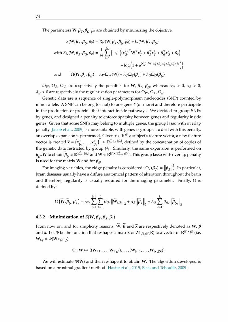
74

The parameters W,βI,βG, β0 are obtained by minimizing the objective:

S(W,βI,βG, β0) = RN(W,βI,βG, β0) +Ω(W,βI,βG)

with RN(W,βI,βG, β0) =1N

N∑k=1

−yk

((xkG)⊤

W⊤xkI + β

⊤IxkI + β

⊤GxkG + β0

)+ log

(1 + e(xk

G)⊤W⊤xkI+β

⊤IxkI+β

⊤GxkG+β0

)and Ω(W,βI,βG) = λWΩW(W) + λIΩI(βI) + λGΩG(βG)

ΩW, ΩI, ΩG are respectively the penalties for W, βI, βG, whereas λW > 0, λI > 0,λG > 0 are respectively the regularization parameters for ΩW, ΩI, ΩG.

Genetic data are a sequence of single-polymorphism nucleotides (SNP) counted byminor allele. A SNP can belong (or not) to one gene ℓ (or more) and therefore participatein the production of proteins that interact inside pathways. We decided to group SNPsby genes, and designed a penalty to enforce sparsity between genes and regularity insidegenes. Given that some SNPs may belong to multiple genes, the group lasso with overlappenalty [Jacob et al., 2009] is more suitable, with genes as groups. To deal with this penalty,an overlap expansion is performed. Given x ∈ R|G| a subject’s feature vector, a new featurevector is created x =

(x⊤G1

, . . . , x⊤GL

)⊤ ∈ R∑Lℓ=1 |Gℓ |, defined by the concatenation of copies of

the genetic data restricted by group Gℓ. Similarly, the same expansion is performed onβG,W to obtain βG ∈ R

∑Lℓ=1 |Gℓ | and W ∈ R|I|×(

∑Lℓ=1 |Gℓ |). This group lasso with overlap penalty

is used for the matrix W and for βG.

For imaging variables, the ridge penalty is considered: ΩI(βI) =∥∥∥βI∥∥∥2

2. In particular,brain diseases usually have a diffuse anatomical pattern of alteration throughout the brainand therefore, regularity is usually required for the imaging parameter. Finally, Ω isdefined by:

Ω(W, βG,βI

)= λW

|I|∑i=1

L∑ℓ=1

θGℓ∥∥∥Wi,Gℓ

∥∥∥2 + λI

∥∥∥∥βI∥∥∥∥2+ λG

L∑ℓ=1

θGℓ

∥∥∥∥βGℓ∥∥∥∥2

4.3.2 Minimization of S(W,βI,βI, β0)

From now on, and for simplicity reasons, W, β and x are respectively denoted as W, βand x. Let Φ be the function that reshapes a matrix ofM|I|,|G|(R) to a vector of R|I|×|G| (i.e.Wi,g = Φ(W)i|G|+g):

Φ : W 7→ ((W1,1, . . . ,W1,|G|), . . . , (W|I|,1, . . . ,W|I|,|G|))

We will estimate Φ(W) and then reshape it to obtain W. The algorithm developed isbased on a proximal gradient method [Hastie et al., 2015, Beck and Teboulle, 2009].

4.3. Model set-up 75

Algorithm 1: Training the multilevel logistic regression

1 Input: (xkI, x

kG, y

k), k = 1, . . . ,N, δ = 0.8, ε0 = 1, η = 10−5 ;2 Initialization: W = 0, βI = 0, βG = 0, β0 = 0, ε = ε0 and converged = False ;3 while not(converged) do4 Compute RN = RN

(W,βI,βG, β0

);

5 Compute ∇RN =1N

N∑k=1

Φ

((xkI)⊤xkG)

xkI

xkG1

[σ((xkG)⊤

W⊤xkI + β

⊤IxkI + β

⊤GxkG + β0

)− yk

]6 Compute ω = β − ε∇(W,βI,βG)RN ;

7 Update WGℓ,i = max

0, 1 − ελGθGℓ∥∥∥∥ω(t)Gℓ+i|G|

∥∥∥∥2

ωGℓ+i|G| for (i, ℓ) ∈ ⟦1, |I|⟧ × ⟦1,L⟧ ;

8 Update βI =ωI+|G||I|1+2ελI

for i ∈ ⟦1, |I|⟧ (imaging modality) ;

9 Update βGℓ = max

0, 1 − ελGθGℓ∥∥∥∥ω(t)Gℓ+(|G|+1)|I|

∥∥∥∥2

ωGℓ+(|G|+1)|I| for ℓ ∈ ⟦1,L⟧ ;

10 Update β0 = β0 − ε∂RN∂β0

and G = 1ε

Φ(W)βIβGβ0

−Φ(W)βIβGβ0

;

11 if RN(W, βI, βG, β0

)> RN − ε∇R⊤NG + ε

2∥G∥22 then12 ε = δε;13 else14 converged =

∣∣∣∣S (W, βI, βG, β0

)− S

(W,βI,βG, β0

)∣∣∣∣<? η∣∣∣∣S (

W,βI,βG, β0

)∣∣∣∣ ;

15 W = W, βI = βI, βG = βG, β0 = β0, ε = ε0 ;16 end17 end18 return

(W,βI,βG, β0

)The parameters w(t+1) =

(Φ

(W(t+1)

),β(t+1)I ,β(t+1)

G , β(t+1)0

)are updated with:

w(t+1) = argminw

RN (w) +[w −w(t)

]⊤ ∇RN(w(t)

)+

12ε

∥∥∥w −w(t)∥∥∥2

2 +Ω(w)

= argminw

12

∥∥∥ω(t) −w(t)∥∥∥2

2 + εΩ(w)

with ω(t) = w(t) − ε∇RN(w(t)

)The idea is to update w(t+1) from w(t) with a Newton-type algorithm without the

constraintΩ given a stepsize ε, and then to project the result onto the compact set definedby Ω. Regarding the stepsize ε, a backtracking line search [Beck and Teboulle, 2009] isperformed. Let G

(w(t), ε

)= 1

ε

[w(t) −w(t+1)

]be the step in the proximal gradient update.

A line search is performed over ε until the inequality is reached:

RN(w(t+1)

)≤ RN

(w(t)

)− ε∇RN

(w(t)

)⊤G

(w(t), ε

)+ε2

∥∥∥∥G(w(t), ε

)∥∥∥∥2

2

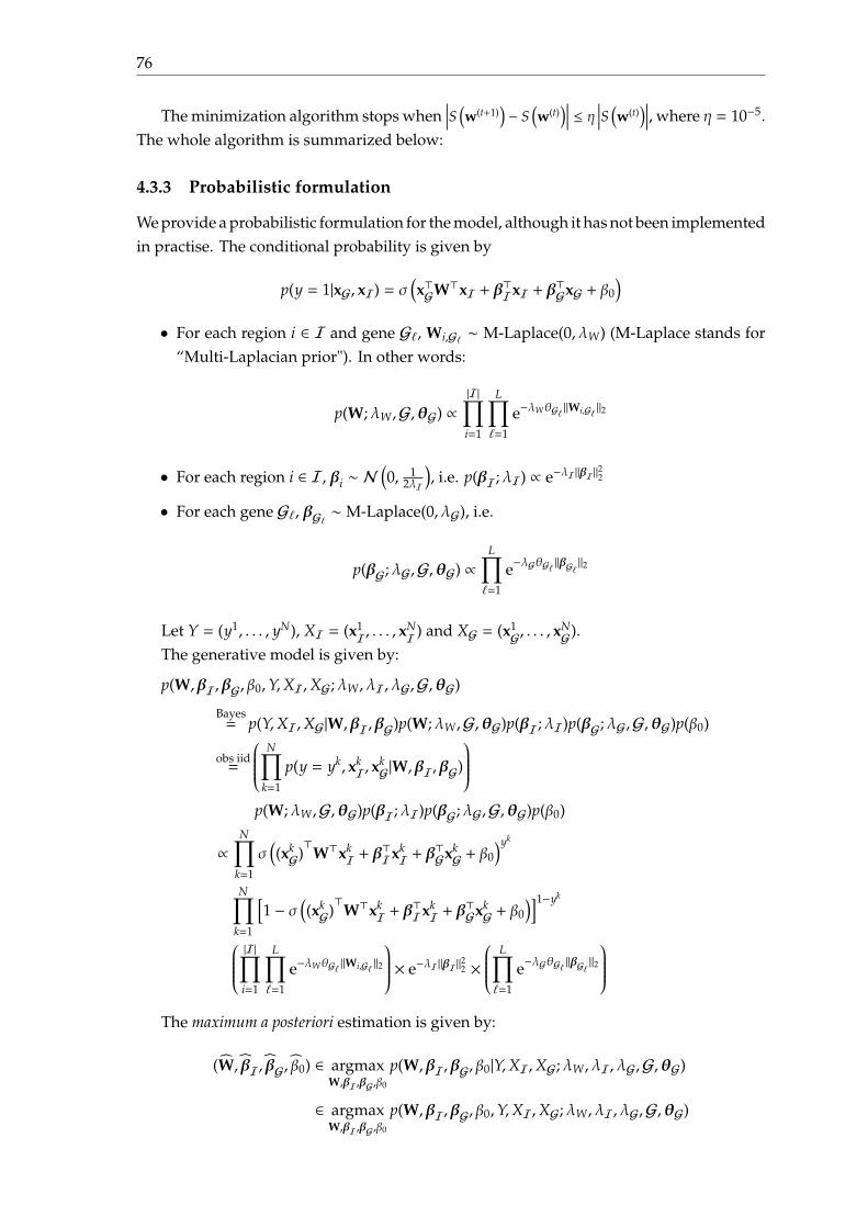
76

The minimization algorithm stops when∣∣∣∣S (

w(t+1))− S

(w(t)

)∣∣∣∣ ≤ η ∣∣∣∣S (w(t)

)∣∣∣∣, where η = 10−5.The whole algorithm is summarized below:

4.3.3 Probabilistic formulation

We provide a probabilistic formulation for the model, although it has not been implementedin practise. The conditional probability is given by

p(y = 1|xG, xI) = σ(x⊤GW⊤xI + β

⊤IxI + β

⊤GxG + β0

)• For each region i ∈ I and gene Gℓ, Wi,Gℓ ∼ M-Laplace(0, λW) (M-Laplace stands for

“Multi-Laplacian prior"). In other words:

p(W;λW,G,θG) ∝|I|∏i=1

L∏ℓ=1

e−λWθGℓ ∥Wi,Gℓ ∥2

• For each region i ∈ I, βi ∼ N(0, 1

2λI

), i.e. p(βI;λI) ∝ e−λI∥βI∥

22

• For each gene Gℓ, βGℓ ∼M-Laplace(0, λG), i.e.

p(βG;λG,G,θG) ∝L∏ℓ=1

e−λGθGℓ ∥βGℓ ∥2

Let Y = (y1, . . . , yN), XI = (x1I, . . . , x

NI ) and XG = (x1

G, . . . , xNG).

The generative model is given by:

p(W,βI,βG, β0,Y,XI,XG;λW, λI, λG,G,θG)

Bayes= p(Y,XI,XG|W,βI,βG)p(W;λW,G,θG)p(βI;λI)p(βG;λG,G,θG)p(β0)

obs iid=

N∏k=1

p(y = yk, xkI, x

kG|W,βI,βG)

p(W;λW,G,θG)p(βI;λI)p(βG;λG,G,θG)p(β0)

∝N∏

k=1

σ((xkG)⊤

W⊤xkI + β

⊤IxkI + β

⊤GxkG + β0

)yk

N∏k=1

[1 − σ

((xkG)⊤

W⊤xkI + β

⊤IxkI + β

⊤GxkG + β0

)]1−yk

|I|∏i=1

L∏ℓ=1

e−λWθGℓ ∥Wi,Gℓ ∥2

× e−λI∥βI∥22 ×

L∏ℓ=1

e−λGθGℓ ∥βGℓ ∥2

The maximum a posteriori estimation is given by:

(W, βI, βG, β0) ∈ argmaxW,βI,βG,β0

p(W,βI,βG, β0|Y,XI,XG;λW, λI, λG,G,θG)

∈ argmaxW,βI,βG,β0

p(W,βI,βG, β0,Y,XI,XG;λW, λI, λG,G,θG)

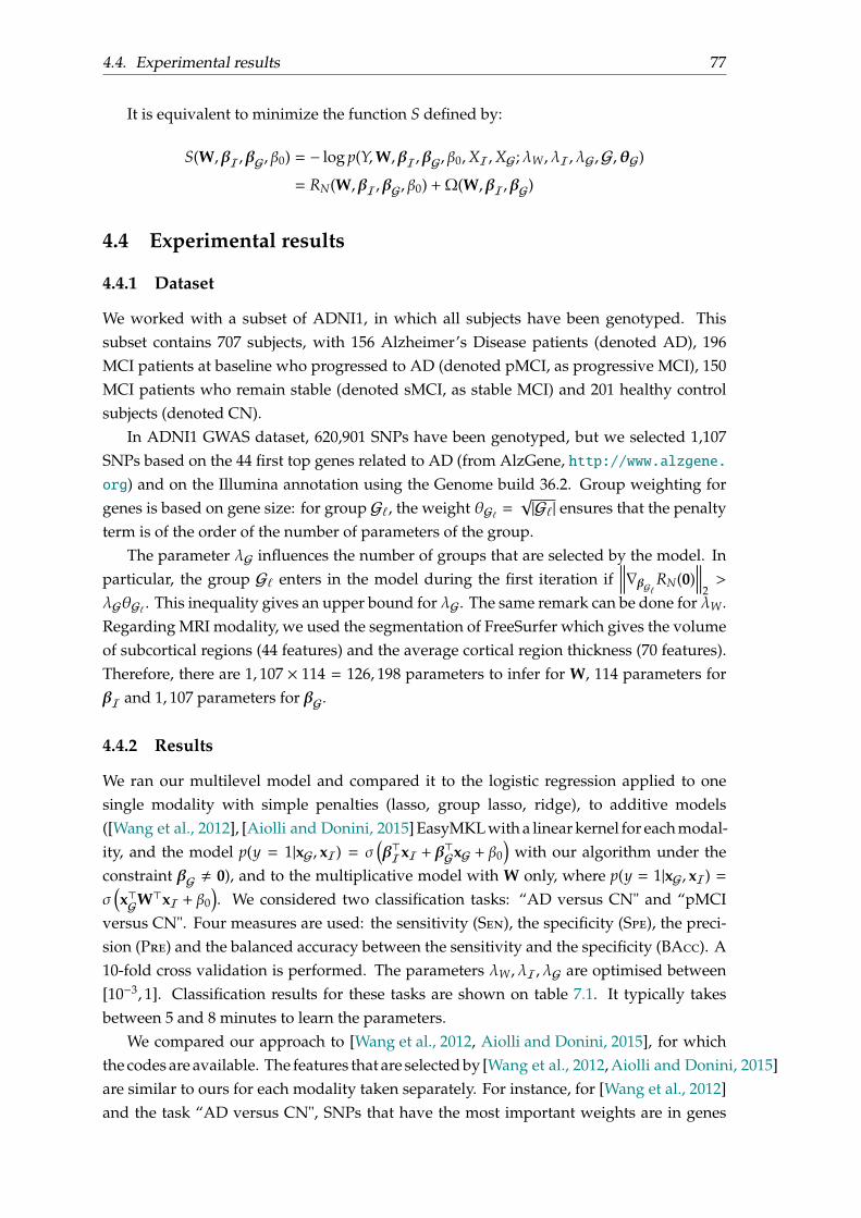
4.4. Experimental results 77

It is equivalent to minimize the function S defined by:

S(W,βI,βG, β0) = − log p(Y,W,βI,βG, β0,XI,XG;λW, λI, λG,G,θG)

= RN(W,βI,βG, β0) +Ω(W,βI,βG)

4.4 Experimental results

4.4.1 Dataset

We worked with a subset of ADNI1, in which all subjects have been genotyped. Thissubset contains 707 subjects, with 156 Alzheimer’s Disease patients (denoted AD), 196MCI patients at baseline who progressed to AD (denoted pMCI, as progressive MCI), 150MCI patients who remain stable (denoted sMCI, as stable MCI) and 201 healthy controlsubjects (denoted CN).

In ADNI1 GWAS dataset, 620,901 SNPs have been genotyped, but we selected 1,107SNPs based on the 44 first top genes related to AD (from AlzGene, http://www.alzgene.org) and on the Illumina annotation using the Genome build 36.2. Group weighting forgenes is based on gene size: for group Gℓ, the weight θGℓ =

√|Gℓ| ensures that the penalty

term is of the order of the number of parameters of the group.The parameter λG influences the number of groups that are selected by the model. In

particular, the group Gℓ enters in the model during the first iteration if∥∥∥∥∇βGℓRN(0)

∥∥∥∥2>

λGθGℓ . This inequality gives an upper bound for λG. The same remark can be done for λW.Regarding MRI modality, we used the segmentation of FreeSurfer which gives the volumeof subcortical regions (44 features) and the average cortical region thickness (70 features).Therefore, there are 1, 107 × 114 = 126, 198 parameters to infer for W, 114 parameters forβI and 1, 107 parameters for βG.

4.4.2 Results

We ran our multilevel model and compared it to the logistic regression applied to onesingle modality with simple penalties (lasso, group lasso, ridge), to additive models([Wang et al., 2012], [Aiolli and Donini, 2015] EasyMKL with a linear kernel for each modal-ity, and the model p(y = 1|xG, xI) = σ

(β⊤IxI + β

⊤GxG + β0

)with our algorithm under the

constraint βG , 0), and to the multiplicative model with W only, where p(y = 1|xG, xI) =σ(x⊤GW⊤xI + β0

). We considered two classification tasks: “AD versus CN" and “pMCI

versus CN". Four measures are used: the sensitivity (Sen), the specificity (Spe), the preci-sion (Pre) and the balanced accuracy between the sensitivity and the specificity (BAcc). A10-fold cross validation is performed. The parameters λW, λI, λG are optimised between[10−3, 1]. Classification results for these tasks are shown on table 7.1. It typically takesbetween 5 and 8 minutes to learn the parameters.

We compared our approach to [Wang et al., 2012, Aiolli and Donini, 2015], for whichthe codes are available. The features that are selected by [Wang et al., 2012, Aiolli and Donini, 2015]are similar to ours for each modality taken separately. For instance, for [Wang et al., 2012]and the task “AD versus CN", SNPs that have the most important weights are in genes

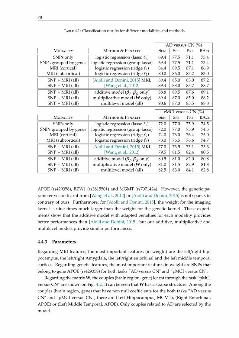
78

Table 4.1: Classification results for different modalities and methods

AD versus CN (%)Modality Method & Penalty Sen Spe Pre BAccSNPs only logistic regression (lasso ℓ1) 69.4 77.5 71.1 73.4

SNPs grouped by genes logistic regression (group lasso) 69.4 77.5 71.1 73.4MRI (cortical) logistic regression (ridge ℓ2) 84.4 89.5 87.1 86.9

MRI (subcortical) logistic regression (ridge ℓ2) 80.0 86.0 83.2 83.0SNP +MRI (all) [Aiolli and Donini, 2015] MKL 89.4 85.0 83.0 87.2SNP +MRI (all) [Wang et al., 2012] 89.4 88.0 85.7 88.7SNP +MRI (all) additive model (βI,βG only) 88.8 89.5 87.6 89.1SNP +MRI (all) multiplicative model (W only) 89.4 87.0 85.0 88.2SNP +MRI (all) multilevel model (all) 90.6 87.0 85.5 88.8

pMCI versus CN (%)Modality Method & Penalty Sen Spe Pre BAccSNPs only logistic regression (lasso ℓ1) 72.0 77.0 75.9 74.5

SNPs grouped by genes logistic regression (group lasso) 72.0 77.0 75.9 74.5MRI (cortical) logistic regression (ridge ℓ2) 74.0 76.0 76.4 75.0

MRI (subcortical) logistic regression (ridge ℓ2) 73.0 76.5 76.6 74.7SNP +MRI (all) [Aiolli and Donini, 2015] MKL 77.0 73.5 75.1 75.3SNP +MRI (all) [Wang et al., 2012] 79.5 81.5 82.4 80.5SNP +MRI (all) additive model (βI,βG only) 80.5 81.0 82.0 80.8SNP +MRI (all) multiplicative model (W only) 81.0 81.5 82.9 81.3SNP +MRI (all) multilevel model (all) 82.5 83.0 84.1 82.8

APOE (rs429358), BZW1 (rs3815501) and MGMT (rs7071424). However, the genetic pa-rameter vector learnt from [Wang et al., 2012] or [Aiolli and Donini, 2015] is not sparse, incontrary of ours. Furthermore, for [Aiolli and Donini, 2015], the weight for the imagingkernel is nine times much larger than the weight for the genetic kernel. These experi-ments show that the additive model with adapted penalties for each modality providesbetter performances than [Aiolli and Donini, 2015], but our additive, multiplicative andmultilevel models provide similar performances.

4.4.3 Parameters

Regarding MRI features, the most important features (in weight) are the left/right hip-pocampus, the left/right Amygdala, the left/right entorhinal and the left middle temporalcortices. Regarding genetic features, the most important features in weight are SNPs thatbelong to gene APOE (rs429358) for both tasks “AD versus CN" and “pMCI versus CN".

Regarding the matrix W, the couples (brain region, gene) learnt through the task “pMCIversus CN" are shown on Fig. 4.2. It can be seen that W has a sparse structure. Among thecouples (brain region, gene) that have non null coefficients for the both tasks “AD versusCN" and “pMCI versus CN", there are (Left Hippocampus, MGMT), (Right Entorhinal,APOE) or (Left Middle Temporal, APOE). Only couples related to AD are selected by themodel.

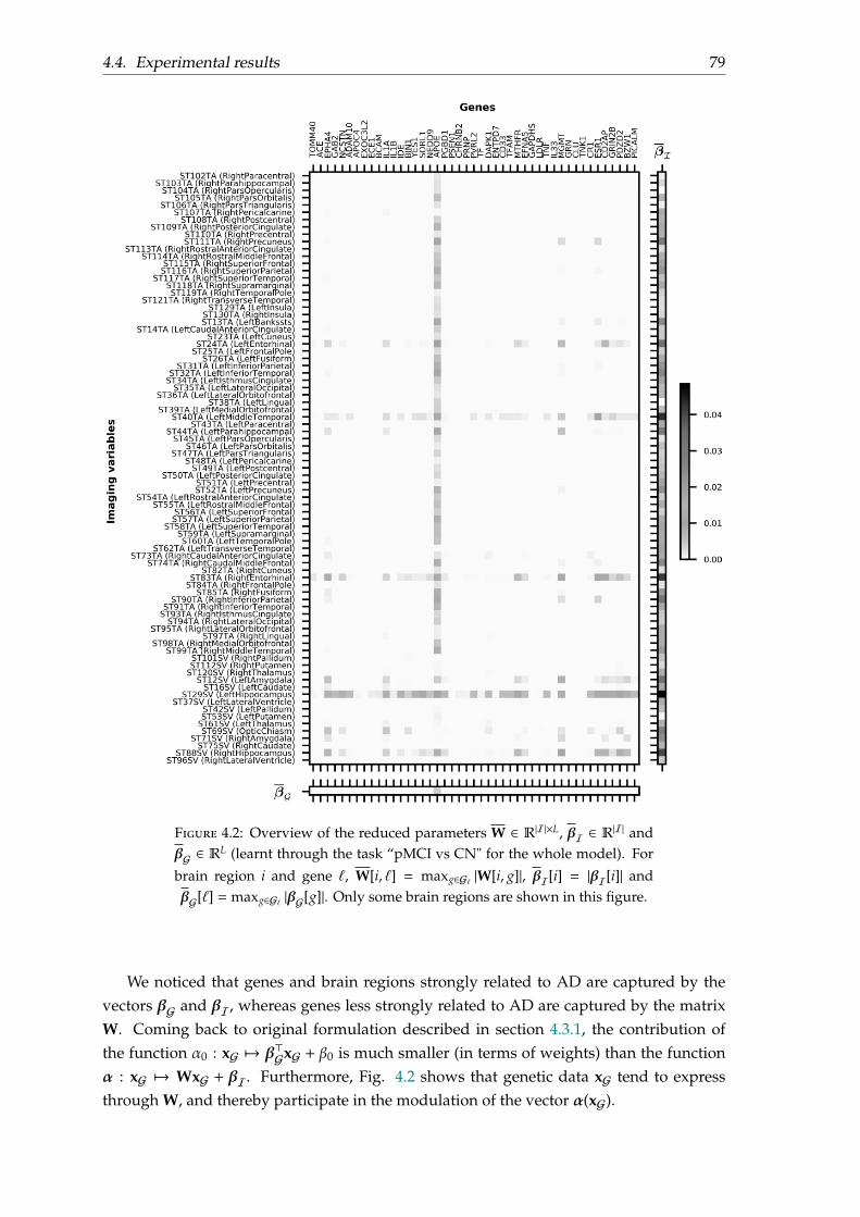
4.4. Experimental results 79

Figure 4.2: Overview of the reduced parameters W ∈ R|I|×L, βI ∈ R|I| andβG ∈ RL (learnt through the task “pMCI vs CN" for the whole model). For

brain region i and gene ℓ, W[i, ℓ] = maxg∈Gℓ |W[i, g]|, βI[i] = |βI[i]| andβG[ℓ] = maxg∈Gℓ |βG[g]|. Only some brain regions are shown in this figure.

We noticed that genes and brain regions strongly related to AD are captured by thevectors βG and βI, whereas genes less strongly related to AD are captured by the matrixW. Coming back to original formulation described in section 4.3.1, the contribution ofthe function α0 : xG 7→ β⊤GxG + β0 is much smaller (in terms of weights) than the functionα : xG 7→ WxG + βI. Furthermore, Fig. 4.2 shows that genetic data xG tend to expressthrough W, and thereby participate in the modulation of the vector α(xG).

80

Figure 4.3 provides another possible interpretation of vector βI and columns of W. Byprojecting the coefficients onto the brain, it is possible to visualise brain regions that arestrongly related to AD (first row), and brain regions, combined with SNP “rs429358" ofAPOE, related to AD (second row).

Another possible visualisation of matrix W is to display a Manhattan plot for someparticular brain regions. In figures 4.4 and 4.5, Manhattan plot for the rows of W corre-sponding to the left entorhinal, the left hippocampus, the left middle temporal and theright entorhinal are shown. These plots highly SNPs that are strongly correlated with thesebrain regions and AD.

Vector βI (intercept)

Column “rs429358" (APOE) of W

Figure 4.3: Intercept βI and slope W in the function α(xG) =WxG + βI

4.5 Conclusion

In this chapter, we developed a novel approach to integrate genetic and brain imagingdata for prediction of disease status. Our multilevel model takes into account potentialinteractions between genes and brain regions, but also the structure of the different typesof data though the use of specific penalties within each modality. When applied to geneticand MRI data from the ADNI database, the model was able to highlight brain regions andgenes that have been previously associated with AD, thereby demonstrating the potentialof our approach for imaging genetics studies in brain diseases.

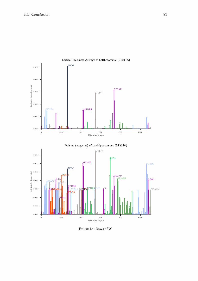
4.5. Conclusion 81

Figure 4.4: Rows of W

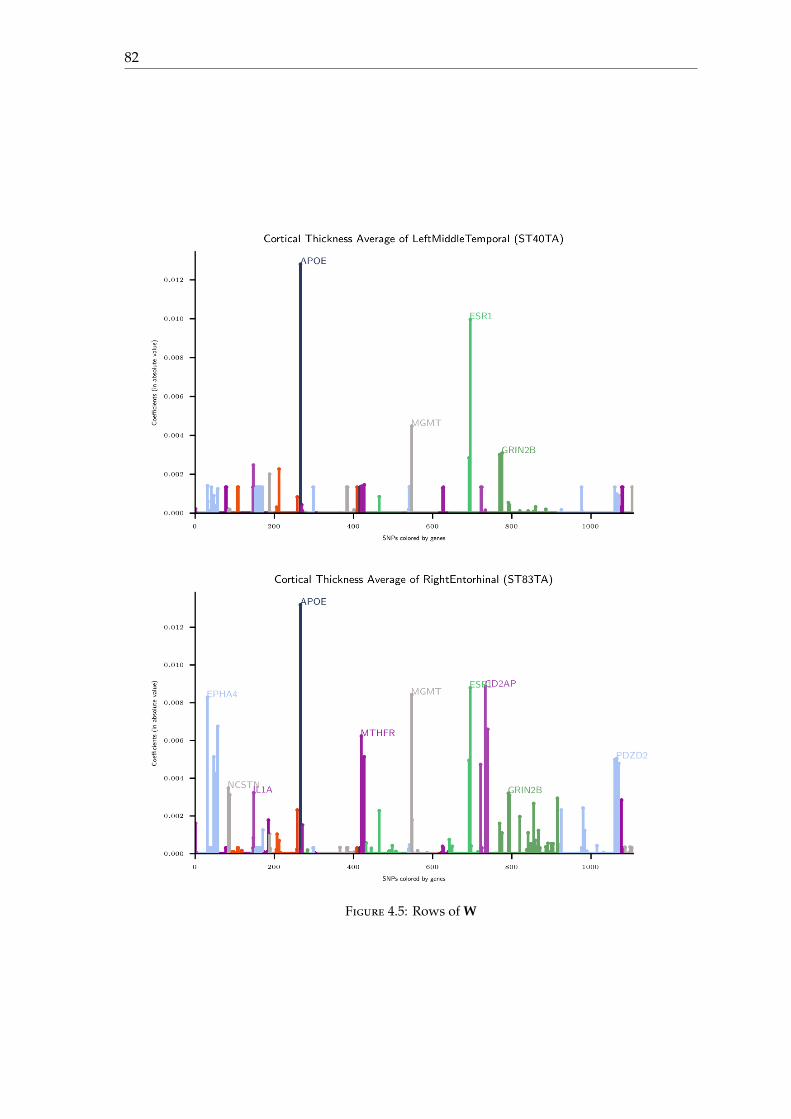
82

Figure 4.5: Rows of W

83

Chapter 5

Contributions to the TADPOLE2017-2022 challenge

5.1 Introduction

The Alzheimer’s Disease Prediction Of Longitudinal Evolution (TADPOLE) Challenge aims atcomparing methods and algorithms at predicting the future evolution of patients at risk ofAlzheimer’s Disease. Details concerning the project are available on their website:

https://tadpole.grand-challenge.org

Launch in 2017, the TADPOLE requires participants to submit their monthly forecasts fora period of 5 years from January 2018 to December 2022.

We start by giving some details on the organisation of the TADPOLE challenge, andthe metrics that they use to assess the performance of each submission. Then, we describeour methodology and contributions to the TADPOLE challenge; and provide some results,after the first phase of evaluation in January 2019.

5.2 Project details

This section is mainly based on [Marinescu et al., 2018].

5.2.1 Overview

TADPOLE Challenge aims at comparing methods and algorithms at predicting the futureevolution of patients at risk of Alzheimer’s Disease. Participants can train their models ondata from the Alzheimer’s Disease Neuroimaging Initiative (ADNI) study or add any otherdatasets. Once the model trained, they have to make monthly forecasts for a period of 5years from January 2018 to December 2022, for all ADNI3 rollover participants. Predictionsthat are asked by TADPOLE are:

• the probabilistic clinical diagnosis, which can be cognitively normal (CN), mild cog-nitive impairment (MCI) or Alzheimer’s disease (AD).

• the cognitive score ADAS-Cog13 (Alzheimer’s Disease Assessment Scale CognitiveSubdomain),

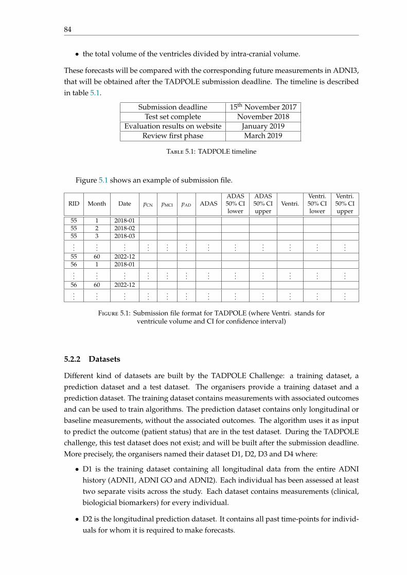
84

• the total volume of the ventricles divided by intra-cranial volume.

These forecasts will be compared with the corresponding future measurements in ADNI3,that will be obtained after the TADPOLE submission deadline. The timeline is describedin table 5.1.

Submission deadline 15th November 2017Test set complete November 2018

Evaluation results on website January 2019Review first phase March 2019

Table 5.1: TADPOLE timeline

Figure 5.1 shows an example of submission file.

RID Month Date pCN pMCI pAD ADASADAS ADAS

Ventri.Ventri. Ventri.

50% CI 50% CI 50% CI 50% CIlower upper lower upper

55 1 2018-0155 2 2018-0255 3 2018-03...

......

......

......

......

......

...55 60 2022-1256 1 2018-01...

......

......

......

......

......

...56 60 2022-12...

......

......

......

......

......

...

Figure 5.1: Submission file format for TADPOLE (where Ventri. stands forventricule volume and CI for confidence interval)

5.2.2 Datasets

Different kind of datasets are built by the TADPOLE Challenge: a training dataset, aprediction dataset and a test dataset. The organisers provide a training dataset and aprediction dataset. The training dataset contains measurements with associated outcomesand can be used to train algorithms. The prediction dataset contains only longitudinal orbaseline measurements, without the associated outcomes. The algorithm uses it as inputto predict the outcome (patient status) that are in the test dataset. During the TADPOLEchallenge, this test dataset does not exist; and will be built after the submission deadline.More precisely, the organisers named their dataset D1, D2, D3 and D4 where:

• D1 is the training dataset containing all longitudinal data from the entire ADNIhistory (ADNI1, ADNI GO and ADNI2). Each individual has been assessed at leasttwo separate visits across the study. Each dataset contains measurements (clinical,biologicial biomarkers) for every individual.

• D2 is the longitudinal prediction dataset. It contains all past time-points for individ-uals for whom it is required to make forecasts.

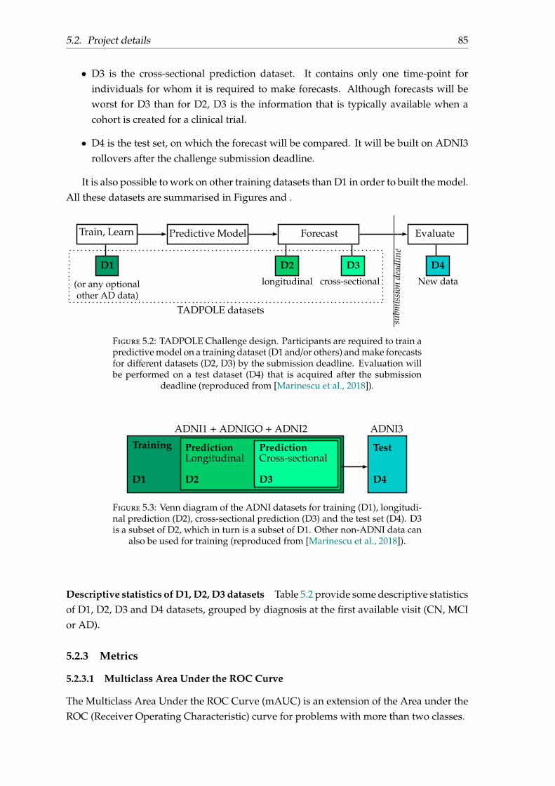
5.2. Project details 85

• D3 is the cross-sectional prediction dataset. It contains only one time-point forindividuals for whom it is required to make forecasts. Although forecasts will beworst for D3 than for D2, D3 is the information that is typically available when acohort is created for a clinical trial.

• D4 is the test set, on which the forecast will be compared. It will be built on ADNI3rollovers after the challenge submission deadline.

It is also possible to work on other training datasets than D1 in order to built the model.All these datasets are summarised in Figures and .

Train, Learn Predictive Model Forecast Evaluate

(or any optionalother AD data)

longitudinal cross-sectional New data

TADPOLE datasets

D4D1 D2 D3

subm

issi

onde

adlin

e

Figure 5.2: TADPOLE Challenge design. Participants are required to train apredictive model on a training dataset (D1 and/or others) and make forecastsfor different datasets (D2, D3) by the submission deadline. Evaluation willbe performed on a test dataset (D4) that is acquired after the submission

deadline (reproduced from [Marinescu et al., 2018]).

ADNI1 + ADNIGO + ADNI2 ADNI3

D1

Training PredictionCross-sectional

D3

Test

D4

PredictionLongitudinal

D2

Figure 5.3: Venn diagram of the ADNI datasets for training (D1), longitudi-nal prediction (D2), cross-sectional prediction (D3) and the test set (D4). D3is a subset of D2, which in turn is a subset of D1. Other non-ADNI data can

also be used for training (reproduced from [Marinescu et al., 2018]).

Descriptive statistics of D1, D2, D3 datasets Table 5.2 provide some descriptive statisticsof D1, D2, D3 and D4 datasets, grouped by diagnosis at the first available visit (CN, MCIor AD).

5.2.3 Metrics

5.2.3.1 Multiclass Area Under the ROC Curve

The Multiclass Area Under the ROC Curve (mAUC) is an extension of the Area under theROC (Receiver Operating Characteristic) curve for problems with more than two classes.

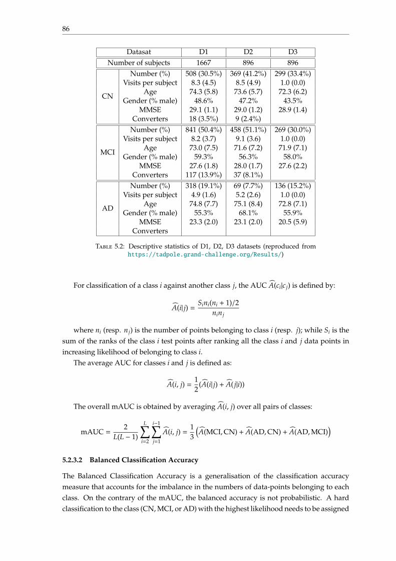
86

Datasat D1 D2 D3Number of subjects 1667 896 896

CN

Number (%) 508 (30.5%) 369 (41.2%) 299 (33.4%)Visits per subject 8.3 (4.5) 8.5 (4.9) 1.0 (0.0)

Age 74.3 (5.8) 73.6 (5.7) 72.3 (6.2)Gender (% male) 48.6% 47.2% 43.5%

MMSE 29.1 (1.1) 29.0 (1.2) 28.9 (1.4)Converters 18 (3.5%) 9 (2.4%)

MCI

Number (%) 841 (50.4%) 458 (51.1%) 269 (30.0%)Visits per subject 8.2 (3.7) 9.1 (3.6) 1.0 (0.0)

Age 73.0 (7.5) 71.6 (7.2) 71.9 (7.1)Gender (% male) 59.3% 56.3% 58.0%

MMSE 27.6 (1.8) 28.0 (1.7) 27.6 (2.2)Converters 117 (13.9%) 37 (8.1%)

AD

Number (%) 318 (19.1%) 69 (7.7%) 136 (15.2%)Visits per subject 4.9 (1.6) 5.2 (2.6) 1.0 (0.0)

Age 74.8 (7.7) 75.1 (8.4) 72.8 (7.1)Gender (% male) 55.3% 68.1% 55.9%

MMSE 23.3 (2.0) 23.1 (2.0) 20.5 (5.9)Converters

Table 5.2: Descriptive statistics of D1, D2, D3 datasets (reproduced fromhttps://tadpole.grand-challenge.org/Results/)

For classification of a class i against another class j, the AUC A(ci|c j) is defined by:

A(i| j) = Sini(ni + 1)/2nin j

where ni (resp. n j) is the number of points belonging to class i (resp. j); while Si is thesum of the ranks of the class i test points after ranking all the class i and j data points inincreasing likelihood of belonging to class i.

The average AUC for classes i and j is defined as:

A(i, j) =12

(A(i| j) + A( j|i))

The overall mAUC is obtained by averaging A(i, j) over all pairs of classes:

mAUC =2

L(L − 1)

L∑i=2

i−1∑j=1

A(i, j) =13

(A(MCI,CN) + A(AD,CN) + A(AD,MCI)

)5.2.3.2 Balanced Classification Accuracy

The Balanced Classification Accuracy is a generalisation of the classification accuracymeasure that accounts for the imbalance in the numbers of data-points belonging to eachclass. On the contrary of the mAUC, the balanced accuracy is not probabilistic. A hardclassification to the class (CN, MCI, or AD) with the highest likelihood needs to be assigned

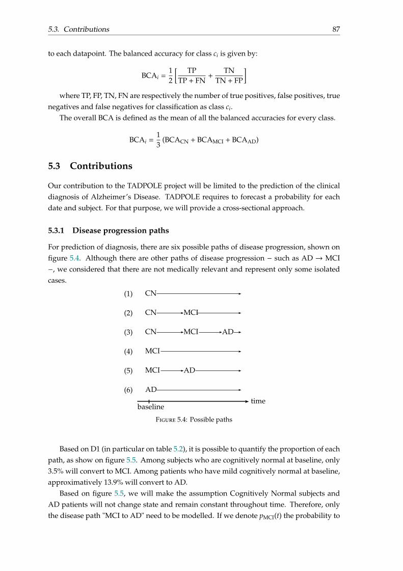
5.3. Contributions 87

to each datapoint. The balanced accuracy for class ci is given by:

BCAi =12

[ TPTP + FN

+TN

TN + FP

]where TP, FP, TN, FN are respectively the number of true positives, false positives, true

negatives and false negatives for classification as class ci.The overall BCA is defined as the mean of all the balanced accuracies for every class.

BCAi =13

(BCACN + BCAMCI + BCAAD)

5.3 Contributions

Our contribution to the TADPOLE project will be limited to the prediction of the clinicaldiagnosis of Alzheimer’s Disease. TADPOLE requires to forecast a probability for eachdate and subject. For that purpose, we will provide a cross-sectional approach.

5.3.1 Disease progression paths

For prediction of diagnosis, there are six possible paths of disease progression, shown onfigure 5.4. Although there are other paths of disease progression − such as AD → MCI−, we considered that there are not medically relevant and represent only some isolatedcases.

CN

CN MCI

ADCN MCI

MCI

MCI AD

AD

(1)

(2)

(3)

(4)

(5)

(6)

baselinetime

Figure 5.4: Possible paths

Based on D1 (in particular on table 5.2), it is possible to quantify the proportion of eachpath, as show on figure 5.5. Among subjects who are cognitively normal at baseline, only3.5% will convert to MCI. Among patients who have mild cognitively normal at baseline,approximatively 13.9% will convert to AD.

Based on figure 5.5, we will make the assumption Cognitively Normal subjects andAD patients will not change state and remain constant throughout time. Therefore, onlythe disease path "MCI to AD" need to be modelled. If we denote pMCI(t) the probability to

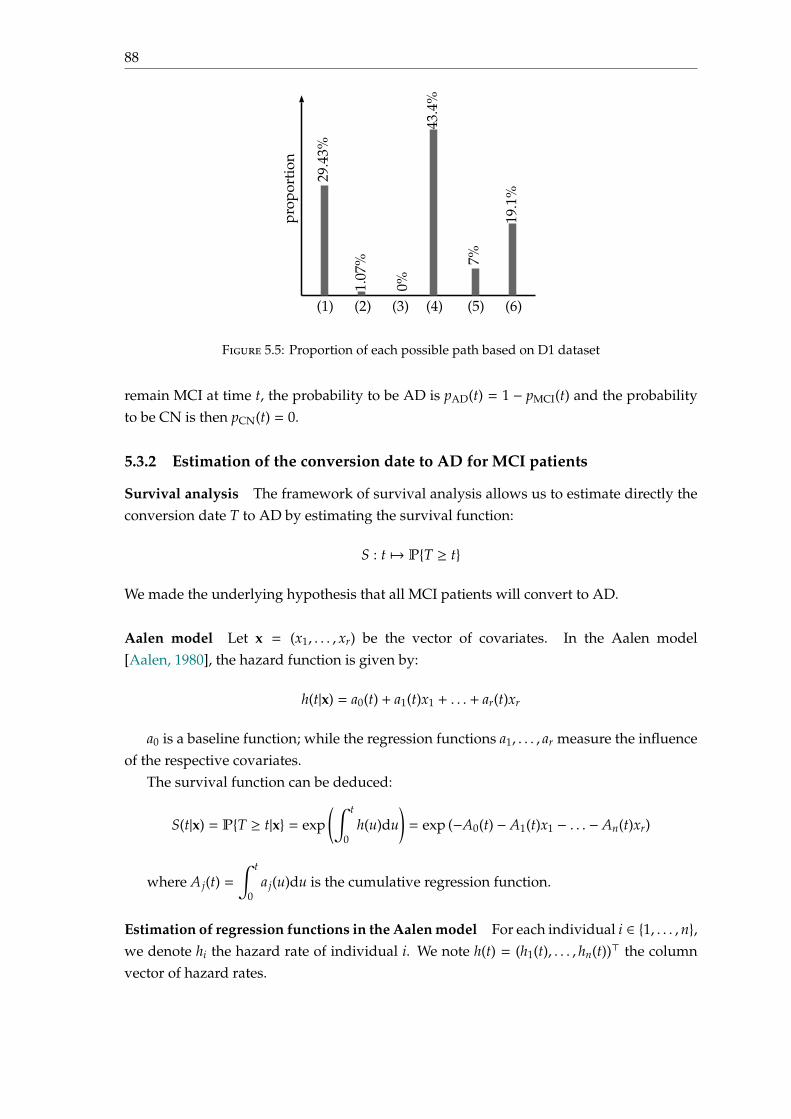
88

(1) (2) (3) (4) (5) (6)pr

opor

tion

29.4

3%

1.07

%

0%

43.4

%

7%

19.1

%

Figure 5.5: Proportion of each possible path based on D1 dataset

remain MCI at time t, the probability to be AD is pAD(t) = 1 − pMCI(t) and the probabilityto be CN is then pCN(t) = 0.

5.3.2 Estimation of the conversion date to AD for MCI patients

Survival analysis The framework of survival analysis allows us to estimate directly theconversion date T to AD by estimating the survival function:

S : t 7→ PT ≥ t

We made the underlying hypothesis that all MCI patients will convert to AD.

Aalen model Let x = (x1, . . . , xr) be the vector of covariates. In the Aalen model[Aalen, 1980], the hazard function is given by:

h(t|x) = a0(t) + a1(t)x1 + . . . + ar(t)xr

a0 is a baseline function; while the regression functions a1, . . . , ar measure the influenceof the respective covariates.

The survival function can be deduced:

S(t|x) = PT ≥ t|x = exp(∫ t

0h(u)du

)= exp (−A0(t) − A1(t)x1 − . . . − An(t)xr)

where A j(t) =∫ t

0a j(u)du is the cumulative regression function.

Estimation of regression functions in the Aalen model For each individual i ∈ 1, . . . , n,we denote hi the hazard rate of individual i. We note h(t) = (h1(t), . . . , hn(t))⊤ the columnvector of hazard rates.

5.3. Contributions 89

The additive model is given by h(t) = Y(t)α(t) where α(t) = (a0(t), a1(t), . . . , ar(t))⊤ is theregression information and Y(t) ∈ Mn,r+1(R) the design matrix where ith row of Y(t) is:

Yi(t) =

(1, xi1, . . . , x

ir) = (1, xi) if the ith individual is a member of the risk set at time t

(0, . . . , 0) otherwise

It is easier to estimate the cumulative regression functions defined by A j(t) =∫ t

0a j(u)du

than a j(t). Let A(t) = (A0(t), . . . ,Ar(t))⊤. A(t) is estimated by an approach similar to theordinary linear modelr:

A(t) =∑

T(k)≤t

X(T(k))Ik

where T(1) < T(2) < . . . are the ordered event times and Ik is a column vector consistingof zeros except for a one in the place corresponding to the subject who experiences an eventat time T(k). The matrix X(t) is a defined as the ordinary least squares inverse of Y(t):

X(t) = (Y(t)⊤Y(t))−1Y(t)⊤

Features We decide to work with cross-sectional data, and use only one time-point foreach subject.

We chose several non-time dependent features such as genetics (APOE4, as some allelesof this gene increase the factor of development of AD) and the level of education (PTEDUCAT).We also took some time-dependent features such as:

• cognitive and clinical scores: CDRSB, ADAS11, ADAS13, MMSE, RAVLT (immediate), FAQ.

• volumetric of the following anatomical structured, calculated using medical reso-nance images: Hippocampus, Ventricles, Whole Brain, Entorhinal, Fusiform, MidTemporal, ICV.

• the sum of mean glucose metabolism uptake in regions of angular, temporal, andposterior cingulate, calculated from PET scans: FDG.

• the concentration of amyloid peptide Aβ-24-1, τ and τ-phosphorylated proteins inthe cerebrospinal fluid (CSF) features: ABETA_UPENNBIOMK9_04_19_17,TAU_UPENNBIOMK9_04_19_17, PTAU_UPENNBIOMK9_04_19_17.

• the subject’s age: AGE.

These time-dependant features provide a good "picture" of the subject’s state at thetime they were acquired. At the end, our model will use 20 relevant features, which are allknown to be associated to AD diagnosis and/or with progression to AD.

We do not apply any pre- or post-processing. Missing values are imputed from theaverage on the population. There is no confounder correction.

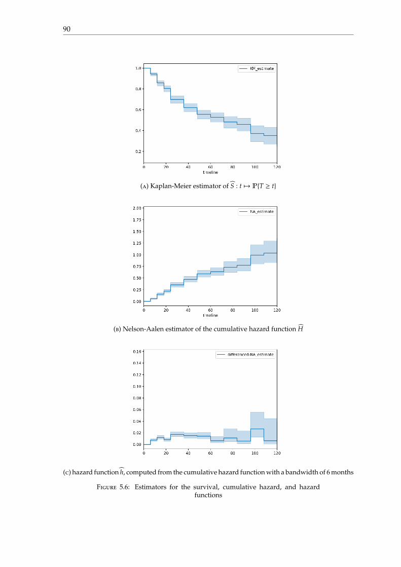
90

(a) Kaplan-Meier estimator of S : t 7→ PT ≥ t

(b) Nelson-Aalen estimator of the cumulative hazard function H

(c) hazard function h, computed from the cumulative hazard function with a bandwidth of 6 months

Figure 5.6: Estimators for the survival, cumulative hazard, and hazardfunctions

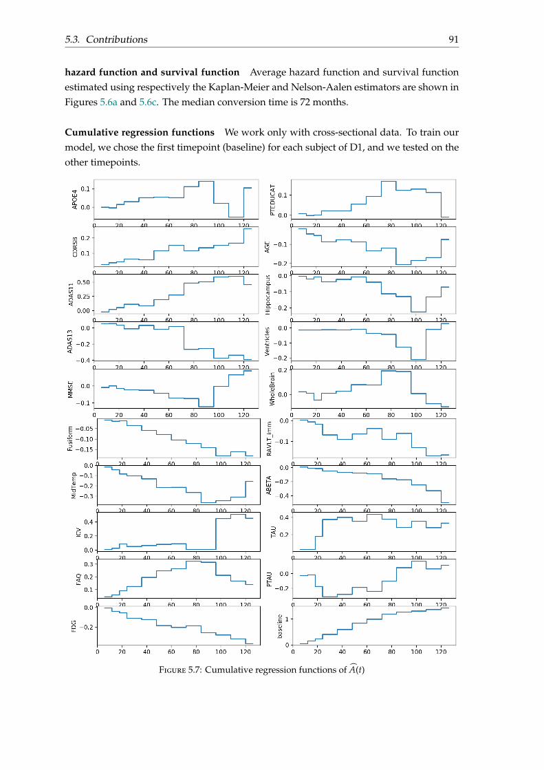
5.3. Contributions 91

hazard function and survival function Average hazard function and survival functionestimated using respectively the Kaplan-Meier and Nelson-Aalen estimators are shown inFigures 5.6a and 5.6c. The median conversion time is 72 months.

Cumulative regression functions We work only with cross-sectional data. To train ourmodel, we chose the first timepoint (baseline) for each subject of D1, and we tested on theother timepoints.

Figure 5.7: Cumulative regression functions of A(t)

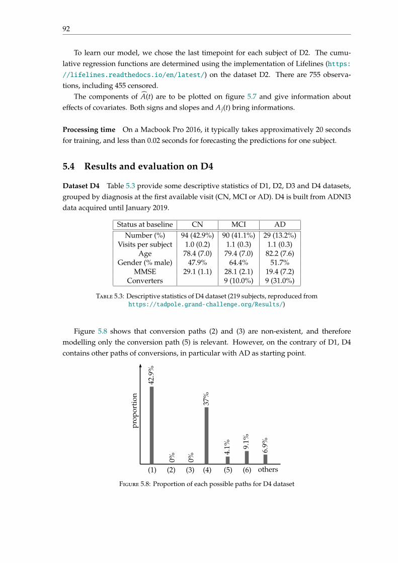
92

To learn our model, we chose the last timepoint for each subject of D2. The cumu-lative regression functions are determined using the implementation of Lifelines (https://lifelines.readthedocs.io/en/latest/) on the dataset D2. There are 755 observa-tions, including 455 censored.

The components of A(t) are to be plotted on figure 5.7 and give information abouteffects of covariates. Both signs and slopes and A j(t) bring informations.

Processing time On a Macbook Pro 2016, it typically takes approximatively 20 secondsfor training, and less than 0.02 seconds for forecasting the predictions for one subject.

5.4 Results and evaluation on D4

Dataset D4 Table 5.3 provide some descriptive statistics of D1, D2, D3 and D4 datasets,grouped by diagnosis at the first available visit (CN, MCI or AD). D4 is built from ADNI3data acquired until January 2019.

Status at baseline CN MCI ADNumber (%) 94 (42.9%) 90 (41.1%) 29 (13.2%)

Visits per subject 1.0 (0.2) 1.1 (0.3) 1.1 (0.3)Age 78.4 (7.0) 79.4 (7.0) 82.2 (7.6)

Gender (% male) 47.9% 64.4% 51.7%MMSE 29.1 (1.1) 28.1 (2.1) 19.4 (7.2)

Converters 9 (10.0%) 9 (31.0%)

Table 5.3: Descriptive statistics of D4 dataset (219 subjects, reproduced fromhttps://tadpole.grand-challenge.org/Results/)

Figure 5.8 shows that conversion paths (2) and (3) are non-existent, and thereforemodelling only the conversion path (5) is relevant. However, on the contrary of D1, D4contains other paths of conversions, in particular with AD as starting point.

(1) (2) (3) (4) (5) (6)

prop

orti

on

42.9

%

0%

37%

4.1% 9.

1%

0%

6.9%

others

Figure 5.8: Proportion of each possible paths for D4 dataset

5.4. Results and evaluation on D4 93

Participating teams and rankings All results are available at:

https://tadpole.grand-challenge.org/Results/

There were a total of 33 participating teams, who submitted a total of 58 forecasts fromD2, 34 forecasts from D3, and 6 forecasts from custom prediction sets. Methods used byparticipating teams are described at:

https://docs.google.com/document/d/

1bh7QoI4Uyz2Q9GMnghmlsJvSlSirI7ttWugmRUGE8ic/edit

The methodology we used was ranked 15th in terms of mAUC (0.876), but came first interms of balanced accuracy (0.85); details results are shown on table 5.4 and 5.5. Althoughour model is a cross-sectional model, we preferred to work with the longitudinal datasetD2 (instead of D3); and used the last timepoint for prediction of dataset D2.

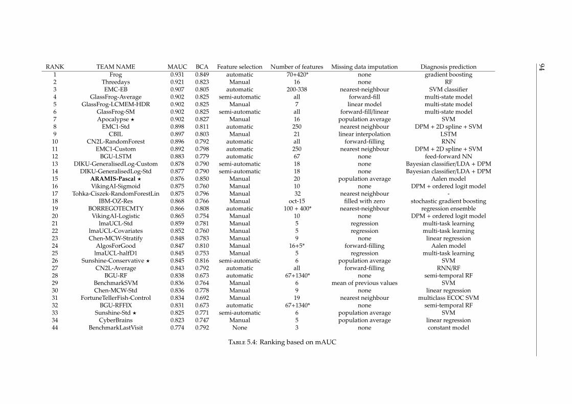
94RANK TEAM NAME MAUC BCA Feature selection Number of features Missing data imputation Diagnosis prediction1 Frog 0.931 0.849 automatic 70+420* none gradient boosting2 Threedays 0.921 0.823 Manual 16 none RF3 EMC-EB 0.907 0.805 automatic 200-338 nearest-neighbour SVM classifier4 GlassFrog-Average 0.902 0.825 semi-automatic all forward-fill multi-state model5 GlassFrog-LCMEM-HDR 0.902 0.825 Manual 7 linear model multi-state model6 GlassFrog-SM 0.902 0.825 semi-automatic all forward-fill/linear multi-state model7 Apocalypse ⋆ 0.902 0.827 Manual 16 population average SVM8 EMC1-Std 0.898 0.811 automatic 250 nearest neighbour DPM + 2D spline + SVM9 CBIL 0.897 0.803 Manual 21 linear interpolation LSTM10 CN2L-RandomForest 0.896 0.792 automatic all forward-filling RNN11 EMC1-Custom 0.892 0.798 automatic 250 nearest neighbour DPM + 2D spline + SVM12 BGU-LSTM 0.883 0.779 automatic 67 none feed-forward NN13 DIKU-GeneralisedLog-Custom 0.878 0.790 semi-automatic 18 none Bayesian classifier/LDA + DPM14 DIKU-GeneralisedLog-Std 0.877 0.790 semi-automatic 18 none Bayesian classifier/LDA + DPM15 ARAMIS-Pascal ⋆ 0.876 0.850 Manual 20 population average Aalen model16 VikingAI-Sigmoid 0.875 0.760 Manual 10 none DPM + ordered logit model17 Tohka-Ciszek-RandomForestLin 0.875 0.796 Manual 32 nearest neighbour -18 IBM-OZ-Res 0.868 0.766 Manual oct-15 filled with zero stochastic gradient boosting19 BORREGOTECMTY 0.866 0.808 automatic 100 + 400* nearest-neighbour regression ensemble20 VikingAI-Logistic 0.865 0.754 Manual 10 none DPM + ordered logit model21 lmaUCL-Std 0.859 0.781 Manual 5 regression multi-task learning22 lmaUCL-Covariates 0.852 0.760 Manual 5 regression multi-task learning23 Chen-MCW-Stratify 0.848 0.783 Manual 9 none linear regression24 AlgosForGood 0.847 0.810 Manual 16+5* forward-filling Aalen model25 lmaUCL-halfD1 0.845 0.753 Manual 5 regression multi-task learning26 Sunshine-Conservative ⋆ 0.845 0.816 semi-automatic 6 population average SVM27 CN2L-Average 0.843 0.792 automatic all forward-filling RNN/RF28 BGU-RF 0.838 0.673 automatic 67+1340* none semi-temporal RF29 BenchmarkSVM 0.836 0.764 Manual 6 mean of previous values SVM30 Chen-MCW-Std 0.836 0.778 Manual 9 none linear regression31 FortuneTellerFish-Control 0.834 0.692 Manual 19 nearest neighbour multiclass ECOC SVM32 BGU-RFFIX 0.831 0.673 automatic 67+1340* none semi-temporal RF33 Sunshine-Std ⋆ 0.825 0.771 semi-automatic 6 population average SVM34 CyberBrains 0.823 0.747 Manual 5 population average linear regression44 BenchmarkLastVisit 0.774 0.792 None 3 none constant model

Table 5.4: Ranking based on mAUC

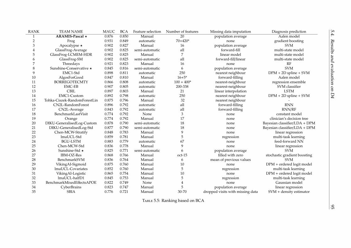
5.4.R

esultsand

evaluationon

D4

95

RANK TEAM NAME MAUC BCA Feature selection Number of features Missing data imputation Diagnosis prediction1 ARAMIS-Pascal ⋆ 0.876 0.850 Manual 20 population average Aalen model2 Frog 0.931 0.849 automatic 70+420* none gradient boosting3 Apocalypse ⋆ 0.902 0.827 Manual 16 population average SVM4 GlassFrog-Average 0.902 0.825 semi-automatic all forward-fill multi-state model5 GlassFrog-LCMEM-HDR 0.902 0.825 Manual 7 linear model multi-state model6 GlassFrog-SM 0.902 0.825 semi-automatic all forward-fill/linear multi-state model7 Threedays 0.921 0.823 Manual 16 none RF8 Sunshine-Conservative ⋆ 0.845 0.816 semi-automatic 6 population average SVM9 EMC1-Std 0.898 0.811 automatic 250 nearest neighbour DPM + 2D spline + SVM

10 AlgosForGood 0.847 0.810 Manual 16+5* forward-filling Aalen model11 BORREGOTECMTY 0.866 0.808 automatic 100 + 400* nearest-neighbour regression ensemble12 EMC-EB 0.907 0.805 automatic 200-338 nearest-neighbour SVM classifier13 CBIL 0.897 0.803 Manual 21 linear interpolation LSTM14 EMC1-Custom 0.892 0.798 automatic 250 nearest neighbour DPM + 2D spline + SVM15 Tohka-Ciszek-RandomForestLin 0.875 0.796 Manual 32 nearest neighbour -16 CN2L-RandomForest 0.896 0.792 automatic all forward-filling RNN17 CN2L-Average 0.843 0.792 automatic all forward-filling RNN/RF18 BenchmarkLastVisit 0.774 0.792 None 3 none constant model19 Orange 0.774 0.792 Manual 17 none clinician’s decision tree20 DIKU-GeneralisedLog-Custom 0.878 0.790 semi-automatic 18 none Bayesian classifier/LDA + DPM21 DIKU-GeneralisedLog-Std 0.877 0.790 semi-automatic 18 none Bayesian classifier/LDA + DPM22 Chen-MCW-Stratify 0.848 0.783 Manual 9 none linear regression23 lmaUCL-Std 0.859 0.781 Manual 5 regression multi-task learning24 BGU-LSTM 0.883 0.779 automatic 67 none feed-forward NN25 Chen-MCW-Std 0.836 0.778 Manual 9 none linear regression26 Sunshine-Std ⋆ 0.825 0.771 semi-automatic 6 population average SVM27 IBM-OZ-Res 0.868 0.766 Manual oct-15 filled with zero stochastic gradient boosting28 BenchmarkSVM 0.836 0.764 Manual 6 mean of previous values SVM29 VikingAI-Sigmoid 0.875 0.760 Manual 10 none DPM + ordered logit model30 lmaUCL-Covariates 0.852 0.760 Manual 5 regression multi-task learning31 VikingAI-Logistic 0.865 0.754 Manual 10 none DPM + ordered logit model32 lmaUCL-halfD1 0.845 0.753 Manual 5 regression multi-task learning33 BenchmarkMixedEffectsAPOE 0.822 0.749 None 4 none Gaussian model34 CyberBrains 0.823 0.747 Manual 5 population average linear regression35 SBIA 0.776 0.721 Manual 30-70 dropped visits with missing data SVM + density estimator

Table 5.5: Ranking based on BCA

96

5.5 Conclusion

Drawing conclusions based on the ranking provided by TADPOLE would be too prema-ture, as the dataset D4 is still in construction until 2022; however it can be noticed thatmaking the assumption that CN subjects remains constant throughout time is valid. Fur-thermore, using few features but relevant features provides results that are as good asusing all features; leading to models that are easy to compute and understand.

Among the best methods for predicting this disease status, there are on the one handsurvival models such as the Aalen model or the multi-state model; and on the other hand,machine learning approaches such as gradient boosting, SVM and random forest.

97

Chapter 6

Multimodal survival models forpredicting the conversion toAlzheimer’s Disease

6.1 Introduction

In this chapter, we focus on the application of survival models for the prediction of theconversion date to AD for MCI patients, using their genetics and clinical data at baseline.By using survival models, we make the underlying assumption that MCI patients convertto AD, but the conversion date to AD is not always observed. Furthermore, in this problem,death can be a competitive risk with AD; however this information remains unknown inthe ADNI1 dataset.

We start by comparing some baseline models for the prediction of AD (classificationat fixed time T, Cox proportional hazard model, Aalen model, log-logistic model) usingbasic multimodal genetics (APOE, gender) and clinical scores (such as MMSE, ADAS13,RAVLT).

Then, we propose a parametric survival model based on multimodal data to estimatethe conversion date to AD from genetics and clinical data. We chose the log-logistic modelwhich provides a parametric framework where the parameters depends on both clinicaland genetic data. The hazard function is unimodal, which seems well-suited to our model.In our proposed formulation, genetic data xG only influences the speed v(xG) at whichthe conversion would happen, whereas clinical data xC influences the initial state of thesubject p(xC). If S denotes the survival function and t1/2 the median survival time, we sett1/2 = p(xC)/v(xG), and S′(t1/2) = −v(xG). By determining v(xG) and p(xC), we are able todetermine the associated survival function S.

Dataset and features In this chapter, we will work with MCI patients at baseline fromthe ADNI1 dataset, whose descriptive statistics are given in chapter . We will select onlyseven representative features which can be grouped into two categories: non-time varyingcovariates (APOE status, gender (man = 0, woman = 1), education) and time-varyingcovariates measured at baseline (MMSE, ADAS13, RAVLT, age).

6.2 Comparison between classification and survival analysis

In this section, features are centred and normalised.

98

6.2.1 Models

Let x = (x1, . . . , xr) be the vector of covariates for a subject.

Cox proportional hazard model The hazard and survival function for the Cox model arerespectively given by:

h(t) = h0(t)eβ⊤x = h0(t)eβ1x1+...+βrxr and S(t) = (S0(t))eβ

⊤x

Log-logistic model The survival function is defined by:

S(t|x) =1

1 + (λ(x)t)p

and the hazard function by:

h(t|x) =pλ(x)(λ(x)t)p−1

1 + (λ(x)t)p

We can set for instance λ(x) = eα0+α1x1+...+αrxr and p = eβ

Aalen additive model The hazard function [Aalen, 1980] is given by:

h(t|x) = a0(t) + a1(t)x1 + . . . + ar(t)xr

where a0 is a baseline function; while the regression functions a1, . . . , ar measure the influ-ence of the respective covariates. The survival function can be deduced:

S(t|x) = PT ≥ t|x = exp(∫ t

0h(u)du

)= exp (−A0(t) − A1(t)x1 − . . . − An(t)xr)

where A j(t) =∫ t

0a j(u)du is the cumulative regression function.

Classification at fixed time T For T ∈ 6, 12, 18, 24, 36, 48, 60, 72, 84, we ran the classicallogistic regression defined by:

Py = 1|T, x = 11 + e−β(T)⊤x−β0(T)

where β(T) is a time-depending vector, and β0(T) is a time-varying intercept. At monthT, the patient i, whose observed date is Ti and if conversion has occurred is represented byδi is included in the model if:

• it did not convert before month T (δi = 0 and Ti ≥ T); its corresponding label is yi = 0.

• it converted before month T (δi = 1 and Ti ≤ T); its corresponding label is yi = 1.

• it converted after month T (δi = 1 and Ti > T); its corresponding label is yi = 0.

At time T, the patient i whose conversion is not observed δi = 0 and followed until Ti < Tis ignored.

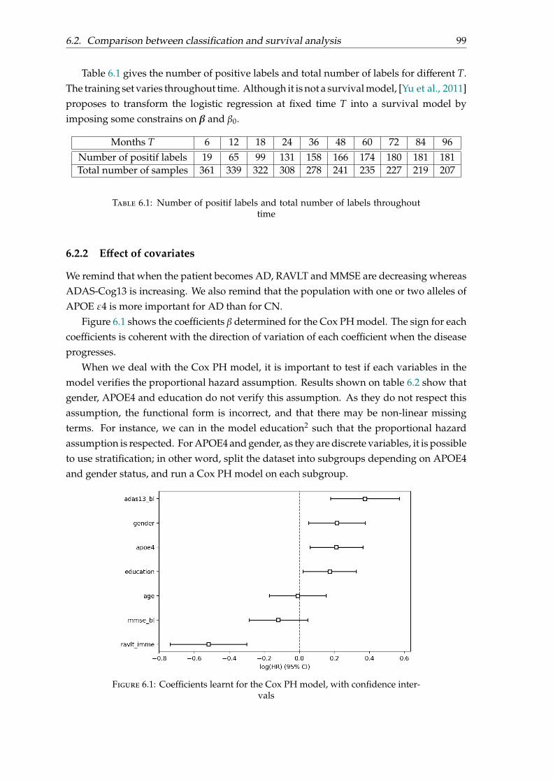
6.2. Comparison between classification and survival analysis 99

Table 6.1 gives the number of positive labels and total number of labels for different T.The training set varies throughout time. Although it is not a survival model, [Yu et al., 2011]proposes to transform the logistic regression at fixed time T into a survival model byimposing some constrains on β and β0.

Months T 6 12 18 24 36 48 60 72 84 96Number of positif labels 19 65 99 131 158 166 174 180 181 181Total number of samples 361 339 322 308 278 241 235 227 219 207

Table 6.1: Number of positif labels and total number of labels throughouttime

6.2.2 Effect of covariates

We remind that when the patient becomes AD, RAVLT and MMSE are decreasing whereasADAS-Cog13 is increasing. We also remind that the population with one or two alleles ofAPOE ε4 is more important for AD than for CN.

Figure 6.1 shows the coefficients β determined for the Cox PH model. The sign for eachcoefficients is coherent with the direction of variation of each coefficient when the diseaseprogresses.

When we deal with the Cox PH model, it is important to test if each variables in themodel verifies the proportional hazard assumption. Results shown on table 6.2 show thatgender, APOE4 and education do not verify this assumption. As they do not respect thisassumption, the functional form is incorrect, and that there may be non-linear missingterms. For instance, we can in the model education2 such that the proportional hazardassumption is respected. For APOE4 and gender, as they are discrete variables, it is possibleto use stratification; in other word, split the dataset into subgroups depending on APOE4and gender status, and run a Cox PH model on each subgroup.

Figure 6.1: Coefficients learnt for the Cox PH model, with confidence inter-vals

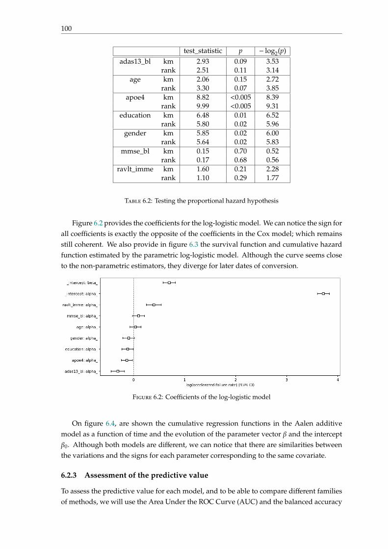
100

test_statistic p − log2(p)adas13_bl km 2.93 0.09 3.53

rank 2.51 0.11 3.14age km 2.06 0.15 2.72

rank 3.30 0.07 3.85apoe4 km 8.82 <0.005 8.39

rank 9.99 <0.005 9.31education km 6.48 0.01 6.52

rank 5.80 0.02 5.96gender km 5.85 0.02 6.00

rank 5.64 0.02 5.83mmse_bl km 0.15 0.70 0.52

rank 0.17 0.68 0.56ravlt_imme km 1.60 0.21 2.28

rank 1.10 0.29 1.77

Table 6.2: Testing the proportional hazard hypothesis

Figure 6.2 provides the coefficients for the log-logistic model. We can notice the sign forall coefficients is exactly the opposite of the coefficients in the Cox model; which remainsstill coherent. We also provide in figure 6.3 the survival function and cumulative hazardfunction estimated by the parametric log-logistic model. Although the curve seems closeto the non-parametric estimators, they diverge for later dates of conversion.

Figure 6.2: Coefficients of the log-logistic model

On figure 6.4, are shown the cumulative regression functions in the Aalen additivemodel as a function of time and the evolution of the parameter vector β and the interceptβ0. Although both models are different, we can notice that there are similarities betweenthe variations and the signs for each parameter corresponding to the same covariate.

6.2.3 Assessment of the predictive value

To assess the predictive value for each model, and to be able to compare different familiesof methods, we will use the Area Under the ROC Curve (AUC) and the balanced accuracy

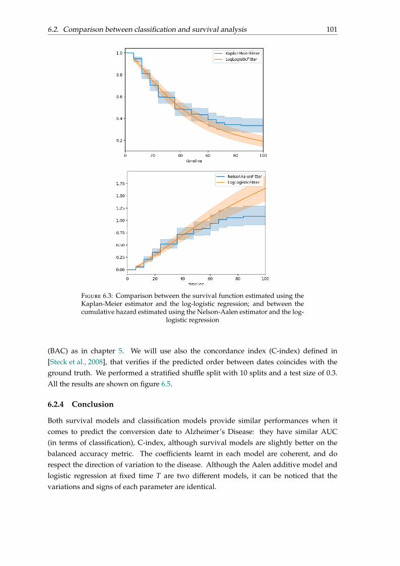
6.2. Comparison between classification and survival analysis 101

Figure 6.3: Comparison between the survival function estimated using theKaplan-Meier estimator and the log-logistic regression; and between thecumulative hazard estimated using the Nelson-Aalen estimator and the log-

logistic regression

(BAC) as in chapter 5. We will use also the concordance index (C-index) defined in[Steck et al., 2008], that verifies if the predicted order between dates coincides with theground truth. We performed a stratified shuffle split with 10 splits and a test size of 0.3.All the results are shown on figure 6.5.

6.2.4 Conclusion

Both survival models and classification models provide similar performances when itcomes to predict the conversion date to Alzheimer’s Disease: they have similar AUC(in terms of classification), C-index, although survival models are slightly better on thebalanced accuracy metric. The coefficients learnt in each model are coherent, and dorespect the direction of variation to the disease. Although the Aalen additive model andlogistic regression at fixed time T are two different models, it can be noticed that thevariations and signs of each parameter are identical.

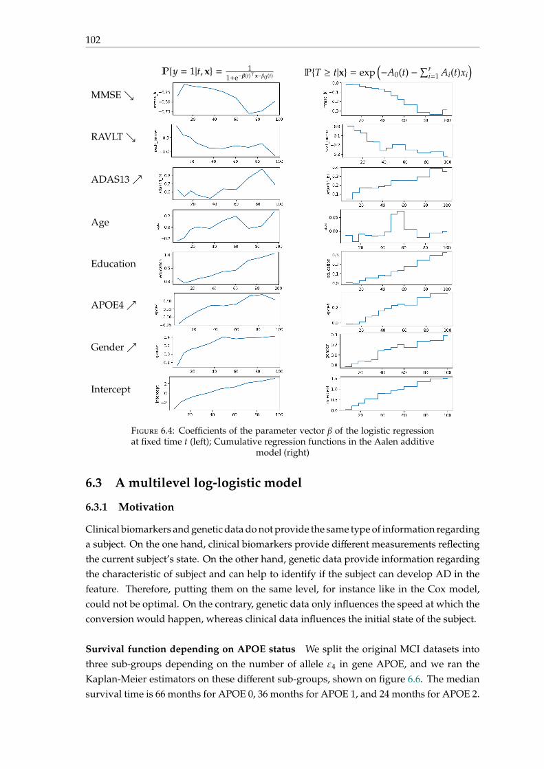
102

Py = 1|t, x = 11+e−β(t)⊤x−β0(t) PT ≥ t|x = exp

(−A0(t) −∑r

i=1 Ai(t)xi

)MMSE

RAVLT

ADAS13

Age

Education

APOE4

Gender

Intercept

Figure 6.4: Coefficients of the parameter vector β of the logistic regressionat fixed time t (left); Cumulative regression functions in the Aalen additive

model (right)

6.3 A multilevel log-logistic model

6.3.1 Motivation

Clinical biomarkers and genetic data do not provide the same type of information regardinga subject. On the one hand, clinical biomarkers provide different measurements reflectingthe current subject’s state. On the other hand, genetic data provide information regardingthe characteristic of subject and can help to identify if the subject can develop AD in thefeature. Therefore, putting them on the same level, for instance like in the Cox model,could not be optimal. On the contrary, genetic data only influences the speed at which theconversion would happen, whereas clinical data influences the initial state of the subject.

Survival function depending on APOE status We split the original MCI datasets intothree sub-groups depending on the number of allele ε4 in gene APOE, and we ran theKaplan-Meier estimators on these different sub-groups, shown on figure 6.6. The mediansurvival time is 66 months for APOE 0, 36 months for APOE 1, and 24 months for APOE 2.

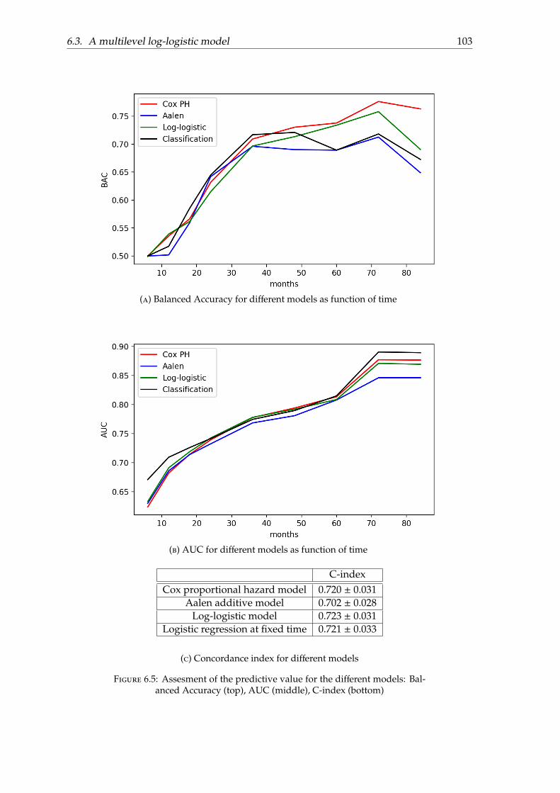
6.3. A multilevel log-logistic model 103

(a) Balanced Accuracy for different models as function of time

(b) AUC for different models as function of time

C-indexCox proportional hazard model 0.720 ± 0.031

Aalen additive model 0.702 ± 0.028Log-logistic model 0.723 ± 0.031

Logistic regression at fixed time 0.721 ± 0.033

(c) Concordance index for different models

Figure 6.5: Assesment of the predictive value for the different models: Bal-anced Accuracy (top), AUC (middle), C-index (bottom)

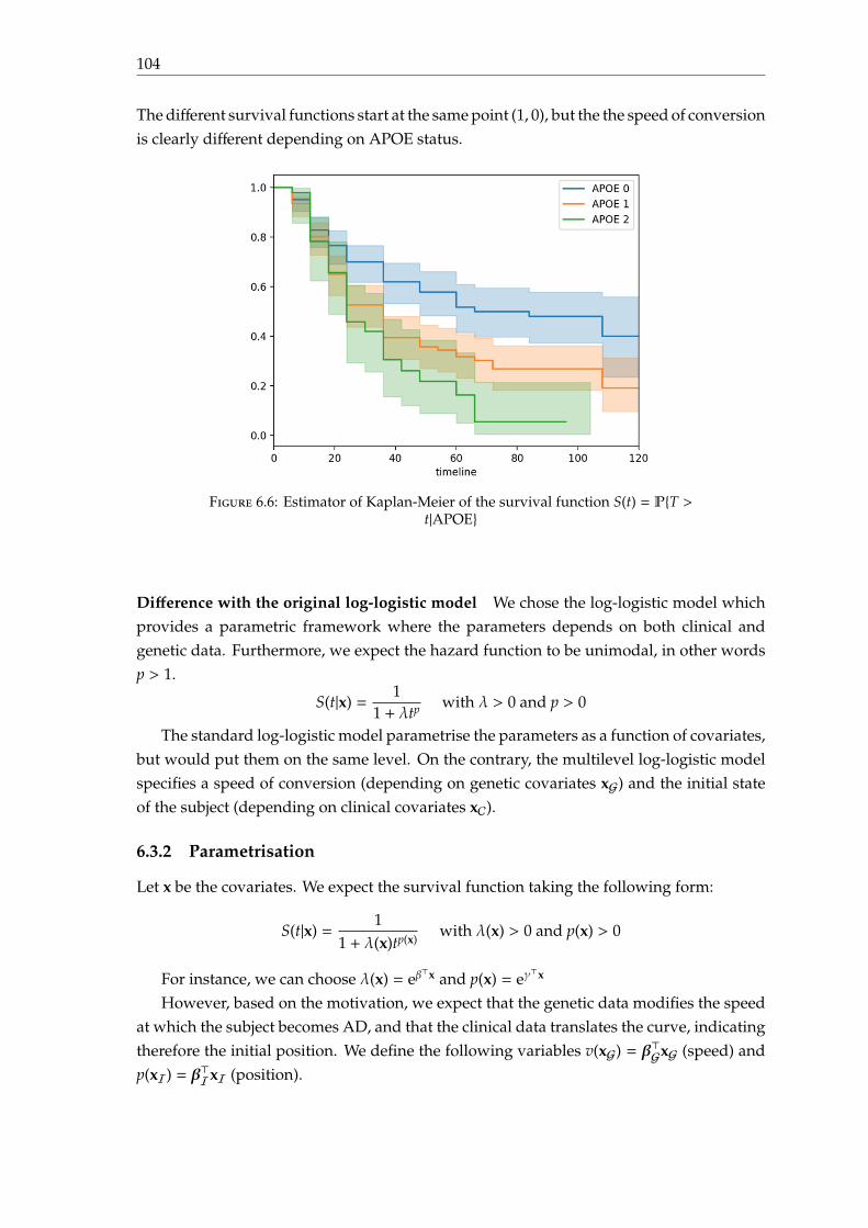
104

The different survival functions start at the same point (1, 0), but the the speed of conversionis clearly different depending on APOE status.

Figure 6.6: Estimator of Kaplan-Meier of the survival function S(t) = PT >t|APOE

Difference with the original log-logistic model We chose the log-logistic model whichprovides a parametric framework where the parameters depends on both clinical andgenetic data. Furthermore, we expect the hazard function to be unimodal, in other wordsp > 1.

S(t|x) =1

1 + λtp with λ > 0 and p > 0

The standard log-logistic model parametrise the parameters as a function of covariates,but would put them on the same level. On the contrary, the multilevel log-logistic modelspecifies a speed of conversion (depending on genetic covariates xG) and the initial stateof the subject (depending on clinical covariates xC).

6.3.2 Parametrisation

Let x be the covariates. We expect the survival function taking the following form:

S(t|x) =1

1 + λ(x)tp(x)with λ(x) > 0 and p(x) > 0

For instance, we can choose λ(x) = eβ⊤x and p(x) = eγ

⊤x

However, based on the motivation, we expect that the genetic data modifies the speedat which the subject becomes AD, and that the clinical data translates the curve, indicatingtherefore the initial position. We define the following variables v(xG) = β⊤GxG (speed) andp(xI) = β⊤IxI (position).

6.3. A multilevel log-logistic model 105

We chose to set the median time t1/2 (the time when S(t) = 12 ) such that:

t1/2 =v(xG)p(xI)

=β⊤GxG

β⊤IxI

and at the median time t1/2, the slope is

S′(t1/2) = −v(xG) = −β⊤GxG

t1/2 =β⊤GxGβ⊤IxI

PT ≥ t

t

0.5

0

b

b

Figure 6.7: Log-logistic model

The conditionsβ⊤GxG > 0 (all subjects convert) andβ⊤IxI > 0 (conversion date is positive)must always be verified.

We start by defining the median time from the model

S(t) = PT ≥ t = 11 + λtp ⇔ t =

(1

S(t)− 1

) 1p 1

λ1p

Then, S(t1/2) = 0.5 gives the following median survival time:

t1/2 =1

λ1p

Furthermore, the density f of T is given by:

f (t) = −S′(t) =λptp−1

(1 + λtp)2

When S(t1/2) = 0.5, then: t1/2 = 1

λ1p

S′(t1/2) = −pλ1p

4 = −p

4t1/2

Therefore: p = −4t1/2S′(t1/2)

λ = 1tp1/2= t4t1/2S′(t1/2)

1/2

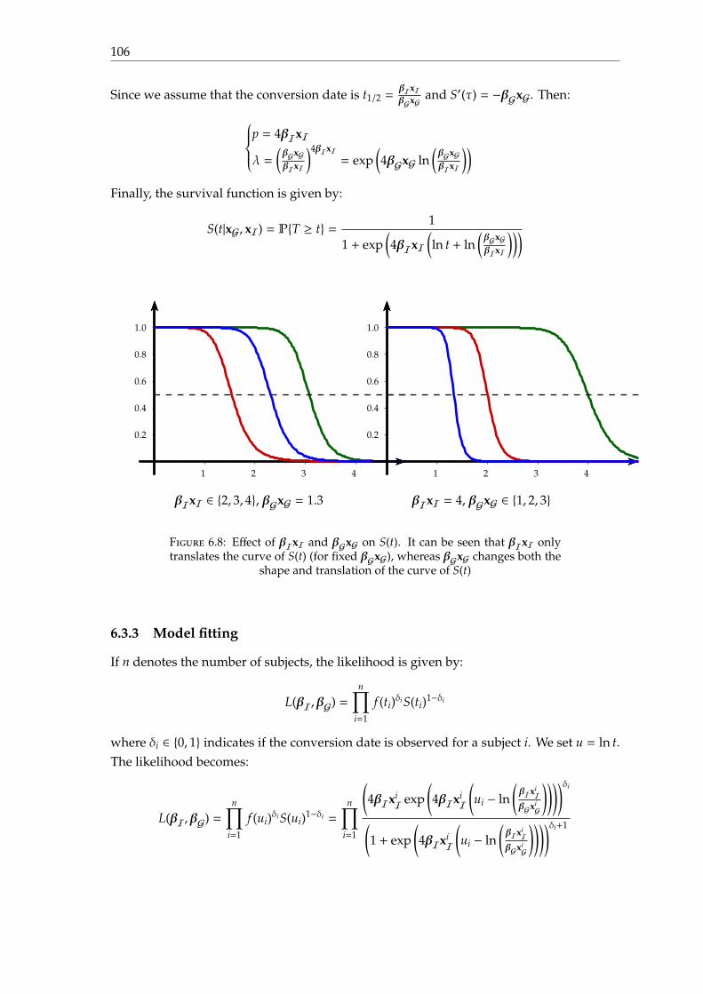
106

Since we assume that the conversion date is t1/2 =βIxIβGxG

and S′(τ) = −βGxG. Then:

p = 4βIxI

λ =(βGxGβIxI

)4βIxI= exp

(4βGxG ln

(βGxGβIxI

))Finally, the survival function is given by:

S(t|xG, xI) = PT ≥ t = 1

1 + exp(4βIxI

(ln t + ln

(βGxGβIxI

)))

0.2

0.4

0.6

0.8

1.0

1 2 3 4

βIxI ∈ 2, 3, 4, βGxG = 1.3

0.2

0.4

0.6

0.8

1.0

1 2 3 4

βIxI = 4, βGxG ∈ 1, 2, 3

Figure 6.8: Effect of βIxI and βGxG on S(t). It can be seen that βIxI onlytranslates the curve of S(t) (for fixed βGxG), whereas βGxG changes both the

shape and translation of the curve of S(t)

6.3.3 Model fitting

If n denotes the number of subjects, the likelihood is given by:

L(βI,βG) =n∏

i=1

f (ti)δiS(ti)1−δi

where δi ∈ 0, 1 indicates if the conversion date is observed for a subject i. We set u = ln t.The likelihood becomes:

L(βI,βG) =n∏

i=1

f (ui)δiS(ui)1−δi =

n∏i=1

(4βIxi

I exp(4βIxi

I

(ui − ln

(βIxi

IβGxi

G

))))δi

(1 + exp

(4βIxi

I

(ui − ln

(βIxi

IβGxi

G

))))δi+1

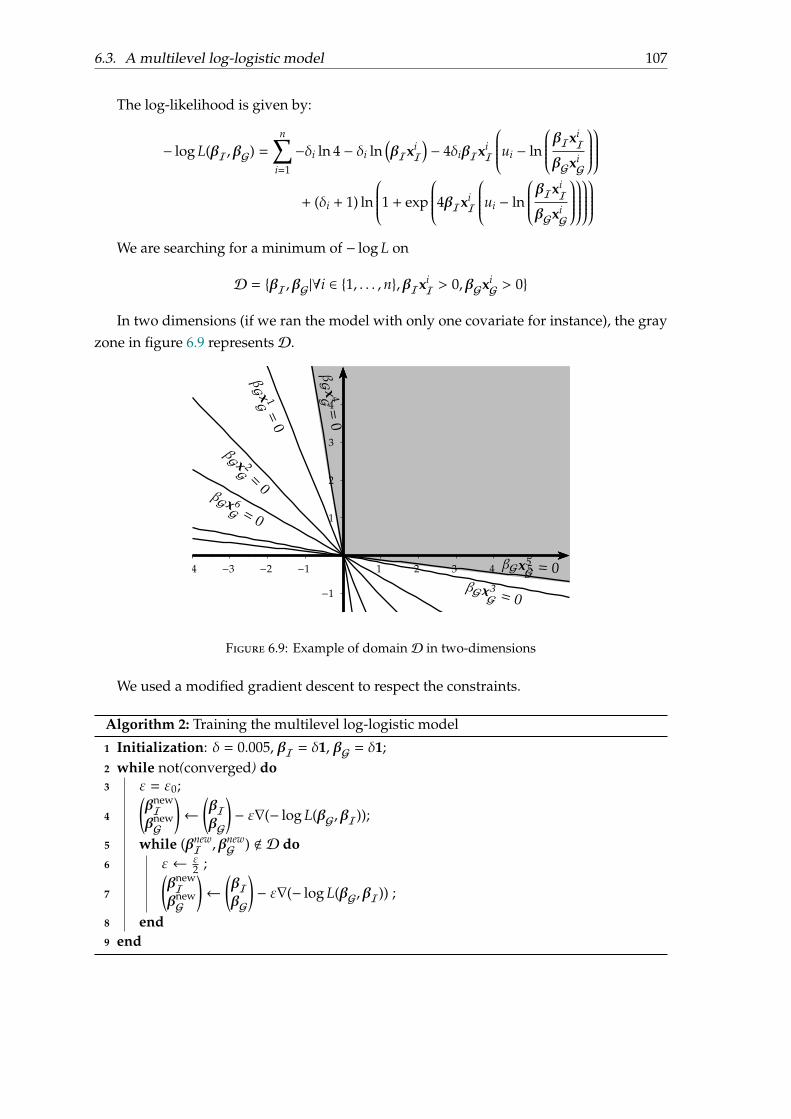
6.3. A multilevel log-logistic model 107

The log-likelihood is given by:

− log L(βI,βG) =n∑

i=1

−δi ln 4 − δi ln(βIxi

I)− 4δiβIxi

I

ui − ln

βIxiI

βGxiG

+ (δi + 1) ln

1 + exp

4βIxiI

ui − ln

βIxiI

βGxiG

We are searching for a minimum of − log L on

D = βI,βG|∀i ∈ 1, . . . , n,βIxiI > 0,βGxi

G > 0

In two dimensions (if we ran the model with only one covariate for instance), the grayzone in figure 6.9 representsD.

−1

−2

1

2

3

4

1 2 3 4 5−1−2−3−4

βG x 1G=

0

βG x 2G =0

βGx3G = 0

βG x 4G=

0

βGx5G = 0

βGx 6G = 0

Figure 6.9: Example of domainD in two-dimensions

We used a modified gradient descent to respect the constraints.

Algorithm 2: Training the multilevel log-logistic model

1 Initialization: δ = 0.005, βI = δ1, βG = δ1;2 while not(converged) do3 ε = ε0;

4

(βnewIβnewG

)←

(βIβG

)− ε∇(− log L(βG,βI));

5 while (βnewI ,βnew

G ) < D do6 ε← ε

2 ;

7

(βnewIβnewG

)←

(βIβG

)− ε∇(− log L(βG,βI)) ;

8 end9 end

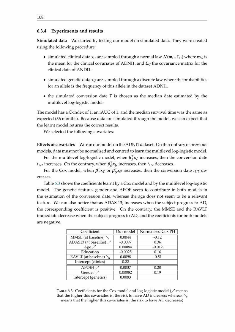
108

6.3.4 Experiments and results

Simulated data We started by testing our model on simulated data. They were createdusing the following procedure:

• simulated clinical data xC are sampled through a normal lawN(mC,ΣC) where mC isthe mean for the clinical covariates of ADNI1, and ΣC the covariance matrix for theclinical data of ANDI1.

• simulated genetic data xG are sampled through a discrete law where the probabilitiesfor an allele is the frequency of this allele in the dataset ADNI1.

• the simulated conversion date T is chosen as the median date estimated by themultilevel log-logistic model.

The model has a C-index of 1, an iAUC of 1, and the median survival time was the same asexpected (36 months). Because data are simulated through the model, we can expect thatthe learnt model returns the correct results.

We selected the following covariates:

Effects of covariates We ran our model on the ADNI1 dataset. On the contrary of previousmodels, data must not be normalised and centred to learn the multilevel log-logistic model.

For the multilevel log-logistic model, when β⊤IxI increases, then the conversion datet1/2 increases. On the contrary, when β⊤GxG increases, then t1/2 decreases.

For the Cox model, when β⊤IxI or β⊤GxG increases, then the conversion date t1/2 de-creases.

Table 6.3 shows the coefficients learnt by a Cox model and by the multilevel log-logisticmodel. The genetic features gender and APOE seem to contribute in both models inthe estimation of the conversion date, whereas the age does not seem to be a relevantfeature. We can also notice that as ADAS 13, increases when the subject progress to AD,the corresponding coefficient is positive. On the contrary, the MMSE and the RAVLTimmediate decrease when the subject progress to AD, and the coefficients for both modelsare negative.

Coefficient Our model Normalised Cox PHMMSE (at baseline) 0.0044 -0.12

ADAS13 (at baseline) -0.0097 0.36Age 0.00084 -0.012

Education -0.0025 0.16RAVLT (at baseline) 0.0098 -0.51

Intercept (clinics) 0.22APOE4 0.0037 0.20Gender 0.00082 0.19

Intercept (genetics) 0.0083

Table 6.3: Coefficients for the Cox model and log-logistic model ( meansthat the higher this covariates is, the risk to have AD increases; whereas

means that the higher this covariates is, the risk to have AD decreases)

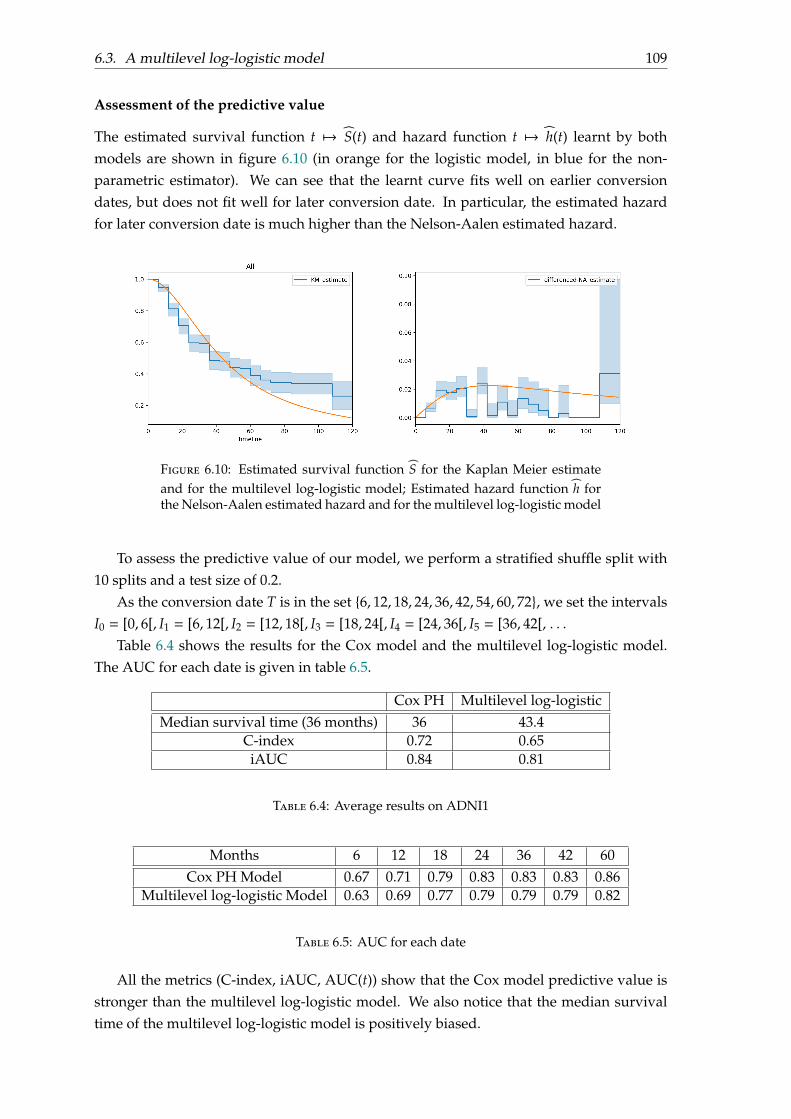
6.3. A multilevel log-logistic model 109

Assessment of the predictive value

The estimated survival function t 7→ S(t) and hazard function t 7→ h(t) learnt by bothmodels are shown in figure 6.10 (in orange for the logistic model, in blue for the non-parametric estimator). We can see that the learnt curve fits well on earlier conversiondates, but does not fit well for later conversion date. In particular, the estimated hazardfor later conversion date is much higher than the Nelson-Aalen estimated hazard.

Figure 6.10: Estimated survival function S for the Kaplan Meier estimateand for the multilevel log-logistic model; Estimated hazard function h forthe Nelson-Aalen estimated hazard and for the multilevel log-logistic model

To assess the predictive value of our model, we perform a stratified shuffle split with10 splits and a test size of 0.2.

As the conversion date T is in the set 6, 12, 18, 24, 36, 42, 54, 60, 72, we set the intervalsI0 = [0, 6[, I1 = [6, 12[, I2 = [12, 18[, I3 = [18, 24[, I4 = [24, 36[, I5 = [36, 42[, . . .

Table 6.4 shows the results for the Cox model and the multilevel log-logistic model.The AUC for each date is given in table 6.5.

Cox PH Multilevel log-logisticMedian survival time (36 months) 36 43.4

C-index 0.72 0.65iAUC 0.84 0.81

Table 6.4: Average results on ADNI1

Months 6 12 18 24 36 42 60Cox PH Model 0.67 0.71 0.79 0.83 0.83 0.83 0.86

Multilevel log-logistic Model 0.63 0.69 0.77 0.79 0.79 0.79 0.82

Table 6.5: AUC for each date

All the metrics (C-index, iAUC, AUC(t)) show that the Cox model predictive value isstronger than the multilevel log-logistic model. We also notice that the median survivaltime of the multilevel log-logistic model is positively biased.

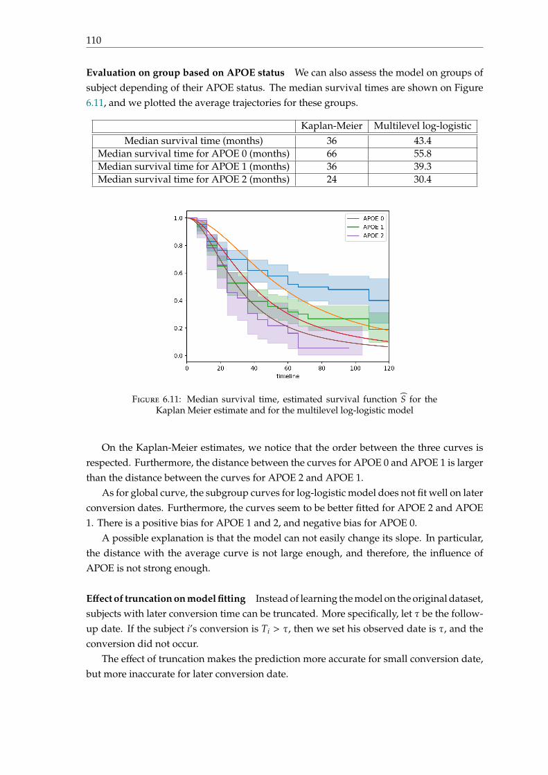
110

Evaluation on group based on APOE status We can also assess the model on groups ofsubject depending of their APOE status. The median survival times are shown on Figure6.11, and we plotted the average trajectories for these groups.

Kaplan-Meier Multilevel log-logisticMedian survival time (months) 36 43.4

Median survival time for APOE 0 (months) 66 55.8Median survival time for APOE 1 (months) 36 39.3Median survival time for APOE 2 (months) 24 30.4

Figure 6.11: Median survival time, estimated survival function S for theKaplan Meier estimate and for the multilevel log-logistic model

On the Kaplan-Meier estimates, we notice that the order between the three curves isrespected. Furthermore, the distance between the curves for APOE 0 and APOE 1 is largerthan the distance between the curves for APOE 2 and APOE 1.

As for global curve, the subgroup curves for log-logistic model does not fit well on laterconversion dates. Furthermore, the curves seem to be better fitted for APOE 2 and APOE1. There is a positive bias for APOE 1 and 2, and negative bias for APOE 0.

A possible explanation is that the model can not easily change its slope. In particular,the distance with the average curve is not large enough, and therefore, the influence ofAPOE is not strong enough.

Effect of truncation on model fitting Instead of learning the model on the original dataset,subjects with later conversion time can be truncated. More specifically, let τ be the follow-up date. If the subject i’s conversion is Ti > τ, then we set his observed date is τ, and theconversion did not occur.

The effect of truncation makes the prediction more accurate for small conversion date,but more inaccurate for later conversion date.

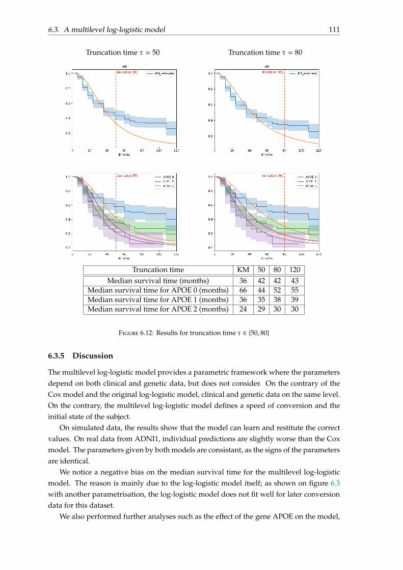
6.3. A multilevel log-logistic model 111

Truncation time τ = 50 Truncation time τ = 80

Truncation time KM 50 80 120Median survival time (months) 36 42 42 43

Median survival time for APOE 0 (months) 66 44 52 55Median survival time for APOE 1 (months) 36 35 38 39Median survival time for APOE 2 (months) 24 29 30 30

Figure 6.12: Results for truncation time τ ∈ 50, 80

6.3.5 Discussion

The multilevel log-logistic model provides a parametric framework where the parametersdepend on both clinical and genetic data, but does not consider. On the contrary of theCox model and the original log-logistic model, clinical and genetic data on the same level.On the contrary, the multilevel log-logistic model defines a speed of conversion and theinitial state of the subject.

On simulated data, the results show that the model can learn and restitute the correctvalues. On real data from ADNI1, individual predictions are slightly worse than the Coxmodel. The parameters given by both models are consistant, as the signs of the parametersare identical.

We notice a negative bias on the median survival time for the multilevel log-logisticmodel. The reason is mainly due to the log-logistic model itself; as shown on figure 6.3with another parametrisation, the log-logistic model does not fit well for later conversiondata for this dataset.

We also performed further analyses such as the effect of the gene APOE on the model,

112

and the effect of truncation on the model’s performance. In particular, the experimentson subgroups of APOE show there is a positive bias for APOE 1 and 2, and negative biasfor APOE 0. An explanation is that the model estimation for genetics can not changeproperly the slope (and the conversion speed), in particular for the subgroup APOE 0.Furthermore, the gap between the survival curve for APOE 0 and the survival curve forAPOE 2 from survival curve for APOE 1 is not identical; as there are much less convertersfor the subgroup APOE 0.

The truncation shows that the model is more accurate on earlier conversion date, andless accurate on later conversion dates. A possible explanation is that there are less dataand less conversions for later conversion dates.

6.4 Conclusion

In the first part of this chapter, we compared different survival models, and a typicalclassification model at fixed time T for the prediction of conversion to Alzheimers Disease.This models (classification at fixed time T, Cox proportional hazard model, Aalen additivemodel, log-logistic model) provide similar results and their coefficients are equivalent.

In the second part of this chapter, we developed a multilevel log-logistic model, wherethe coefficients of the model define a speed of conversion and an initial state. This modelis simple to implement and test. However, it has a strong bias for long conversion dates,due to the log-logistic model, and strong biais for subgroups of population based on theirAPOE status.

113

Chapter 7

Multilevel Cox Proportional hazardModel with Structured Penalties forImaging Genetics data

This chapter is a modified version of:

Lu Pascal, Colliot Olivier. Multilevel Survival Analysis with Structured Penal-ties for Imaging Genetics data. Accepted at SPIE 2020 Medical Imaging.

7.1 Introduction

Predicting the future occurrence of Alzheimer’s Disease (AD) in patients with mild cog-nitive impairment (MCI) is a topic of active research. Many papers have formulated thisquestion as a classification problem: one considers a fixed time of conversion and aims todiscriminate between the patients who have converted to AD at that time and those whohave not. However, a clinically more relevant question is to predict the date at which apatient will convert to AD. Survival analysis is an adequate statistical framework for sucha task.

Multimodal data (imaging and genetic) provide complementary information for theprediction. While imaging data provides an estimate of the current patient’s state, geneticvariants can be associated to the speed of progression to AD. Although they do not providethe same type of information, most papers in classification or regression put imaging andgenetic variables on the same level in order to predict the current or future patient’s state.

In this chapter, we propose a survival model using multimodal data to estimate theconversion date to AD, by considering joint effects between the imaging and geneticmodalities. We use an adapted penalty in the survival model, the group lasso penalty, overjoint groups of genes and brain regions, as in the chapter

The model is evaluated on genetic (single nucleotide polymorphisms) and imaging(anatomical MRI measures) data from the ADNI1 database, and compared to a standardCox PH model.

114

7.2 State of the art

Early diagnosis of Alzheimer’s disease (AD) is an active issue in medical imaging. InAlzheimer’s disease, the group of patients with mild cognitive impairment is heteroge-neous, some are more likely than others to convert to AD; and therefore giving an accuratediagnosis can be difficult [Marinescu et al., 2018]. In this paper, we focus on predictingaccurately the conversion to AD given only one time-point.

Most existing approaches to predict the conversion define the problem as a classifica-tion task at fixed time [Rathore et al., 2017, Cheng et al., 2015, Davatzikos et al., 2011]. Theproblem of using classification at a fixed time is that we have to arbitrarily choose a date atwhich the conversion to AD is observed, we create two groups of homogeneous patients(converting before or after the fixed date), and we do not ensure that conversion in time ismonotonous.

Survival models provide a regression framework which directly estimates the conver-sion date using only one time-point. However, by using survival models, we make severalhypotheses: the conversion event is sometimes not observed (because the study endedbefore conversion), sometimes never occurs (some patients will never convert to AD), andonly happens once. For all patients in the study, the starting point is the entry in the study,and the conversion is the time of progression of the disease to AD.

In a single visit, several kind of data can be acquired (clinical data, neuroimages, fluidbiomarkers, genetic data. . .). Some data, such as clinical data or neuroimaging data providea picture of the patient’s state at the time they were acquired [Rathore et al., 2017]. On thecontrary, others data, such as genetic data, help to identify whether or not a patient coulddevelop AD in the future (for instance, some alleles of APOE increase the risk of developingAD). An issue raised by collecting data from different sources concerns their combination.In the area of imaging genetics, most papers focus either on the association between neu-roimaging covariates and genetic data [Liu and Calhoun, 2014, Batmanghelich et al., 2016],or on building machine learning predictors for a disease at fixed time using classification(logistic regression, SVM [Peng et al., 2016]). All these models combine neuroimaging andgenetic data by using an additive framework. However, adding the effect of both modali-ties and putting them on the same level is not optimal, as these modalities do not providethe same type of information. We proposed a multilevel framework for combining imagingand genetic data for classification.

In this paper, we propose a survival model, based on the Cox Proportional Hazardmodel and using a multilevel framework, as in chapter 4. Survival models (Cox Propor-tional Hazard model) have been applied for combining multimodal data [Bøvelstad et al., 2009]and for predicting the conversion to AD [Li et al., 2017, Anderson et al., 2016, Liu et al., 2017];in both case using an additive framework. Learning the conversion date to AD with modal-ities taken separately shows that the genetic modality has weaker predictive value thanthe neuroimaging modality. Instead of summing both genetic and neuroimaging contribu-tions (which could lead to a weaker contribution of the genetic modality in the model), wepropose that the parameters, combined with the neuroimaging covariates, could be mod-ulated by the patient’s genetic data. This hypothesis leads to a multilevel model where

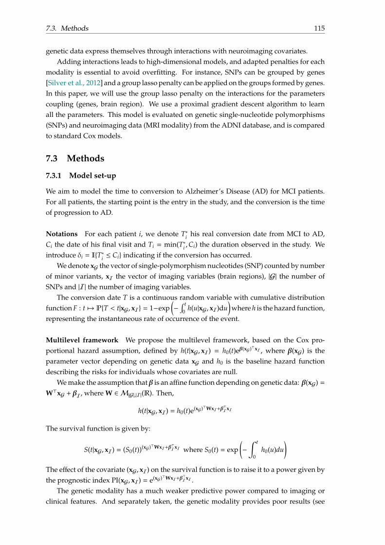
7.3. Methods 115

genetic data express themselves through interactions with neuroimaging covariates.Adding interactions leads to high-dimensional models, and adapted penalties for each

modality is essential to avoid overfitting. For instance, SNPs can be grouped by genes[Silver et al., 2012] and a group lasso penalty can be applied on the groups formed by genes.In this paper, we will use the group lasso penalty on the interactions for the parameterscoupling (genes, brain region). We use a proximal gradient descent algorithm to learnall the parameters. This model is evaluated on genetic single-nucleotide polymorphisms(SNPs) and neuroimaging data (MRI modality) from the ADNI database, and is comparedto standard Cox models.

7.3 Methods

7.3.1 Model set-up

We aim to model the time to conversion to Alzheimer’s Disease (AD) for MCI patients.For all patients, the starting point is the entry in the study, and the conversion is the timeof progression to AD.

Notations For each patient i, we denote T∗i his real conversion date from MCI to AD,Ci the date of his final visit and Ti = min(T∗i ,Ci) the duration observed in the study. Weintroduce δi = IT∗i ≤ Ci indicating if the conversion has occurred.

We denote xG the vector of single-polymorphism nucleotides (SNP) counted by numberof minor variants, xI the vector of imaging variables (brain regions), |G| the number ofSNPs and |I| the number of imaging variables.

The conversion date T is a continuous random variable with cumulative distributionfunction F : t 7→ PT < t|xG, xI = 1−exp

(−

∫ t0 h(u|xG, xI)du

)where h is the hazard function,

representing the instantaneous rate of occurrence of the event.

Multilevel framework We propose the multilevel framework, based on the Cox pro-portional hazard assumption, defined by h(t|xG, xI) = h0(t)eβ(xG)⊤xI , where β(xG) is theparameter vector depending on genetic data xG and h0 is the baseline hazard functiondescribing the risks for individuals whose covariates are null.

We make the assumption that β is an affine function depending on genetic data: β(xG) =W⊤xG + βI, where W ∈ M|G|,|I|(R). Then,

h(t|xG, xI) = h0(t)e(xG)⊤WxI+β⊤IxI

The survival function is given by:

S(t|xG, xI) = (S0(t))(xG)⊤WxI+β⊤IxI where S0(t) = exp

(−

∫ t

0h0(u)du

)The effect of the covariate (xG, xI) on the survival function is to raise it to a power given bythe prognostic index PI(xG, xI) = e(xG)⊤WxI+β

⊤IxI .

The genetic modality has a much weaker predictive power compared to imaging orclinical features. And separately taken, the genetic modality provides poor results (see

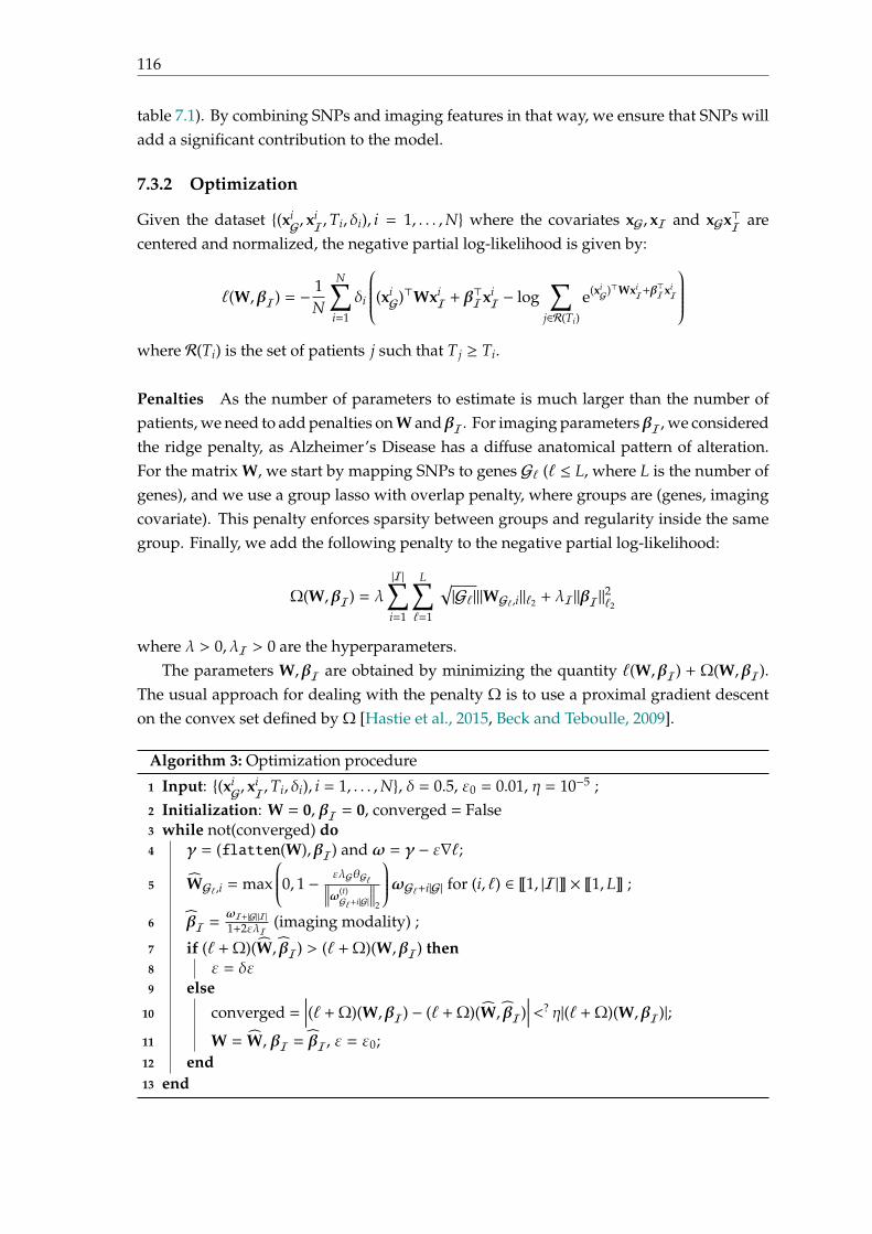
116

table 7.1). By combining SNPs and imaging features in that way, we ensure that SNPs willadd a significant contribution to the model.

7.3.2 Optimization

Given the dataset (xiG, x

iI,Ti, δi), i = 1, . . . ,N where the covariates xG, xI and xGx⊤I are

centered and normalized, the negative partial log-likelihood is given by:

ℓ(W,βI) = − 1N

N∑i=1

δi

(xiG)⊤Wxi

I + β⊤IxiI − log

∑j∈R(Ti)

e(xiG)⊤Wxi

I+β⊤IxiI

where R(Ti) is the set of patients j such that T j ≥ Ti.

Penalties As the number of parameters to estimate is much larger than the number ofpatients, we need to add penalties on W and βI. For imaging parameters βI, we consideredthe ridge penalty, as Alzheimer’s Disease has a diffuse anatomical pattern of alteration.For the matrix W, we start by mapping SNPs to genes Gℓ (ℓ ≤ L, where L is the number ofgenes), and we use a group lasso with overlap penalty, where groups are (genes, imagingcovariate). This penalty enforces sparsity between groups and regularity inside the samegroup. Finally, we add the following penalty to the negative partial log-likelihood:

Ω(W,βI) = λ|I|∑i=1

L∑ℓ=1

√|Gℓ|∥WGℓ,i∥ℓ2 + λI∥βI∥2ℓ2

where λ > 0, λI > 0 are the hyperparameters.The parameters W,βI are obtained by minimizing the quantity ℓ(W,βI) + Ω(W,βI).

The usual approach for dealing with the penalty Ω is to use a proximal gradient descenton the convex set defined by Ω [Hastie et al., 2015, Beck and Teboulle, 2009].

Algorithm 3: Optimization procedure

1 Input: (xiG, x

iI,Ti, δi), i = 1, . . . ,N, δ = 0.5, ε0 = 0.01, η = 10−5 ;

2 Initialization: W = 0, βI = 0, converged = False3 while not(converged) do4 γ = (flatten(W),βI) and ω = γ − ε∇ℓ;

5 WGℓ,i = max

0, 1 − ελGθGℓ∥∥∥∥ω(t)Gℓ+i|G|

∥∥∥∥2

ωGℓ+i|G| for (i, ℓ) ∈ ⟦1, |I|⟧ × ⟦1,L⟧ ;

6 βI =ωI+|G||I|1+2ελI

(imaging modality) ;

7 if (ℓ +Ω)(W, βI) > (ℓ +Ω)(W,βI) then8 ε = δε9 else

10 converged =∣∣∣∣(ℓ +Ω)(W,βI) − (ℓ +Ω)(W, βI)

∣∣∣∣<? η|(ℓ +Ω)(W,βI)|;11 W = W, βI = βI, ε = ε0;12 end13 end

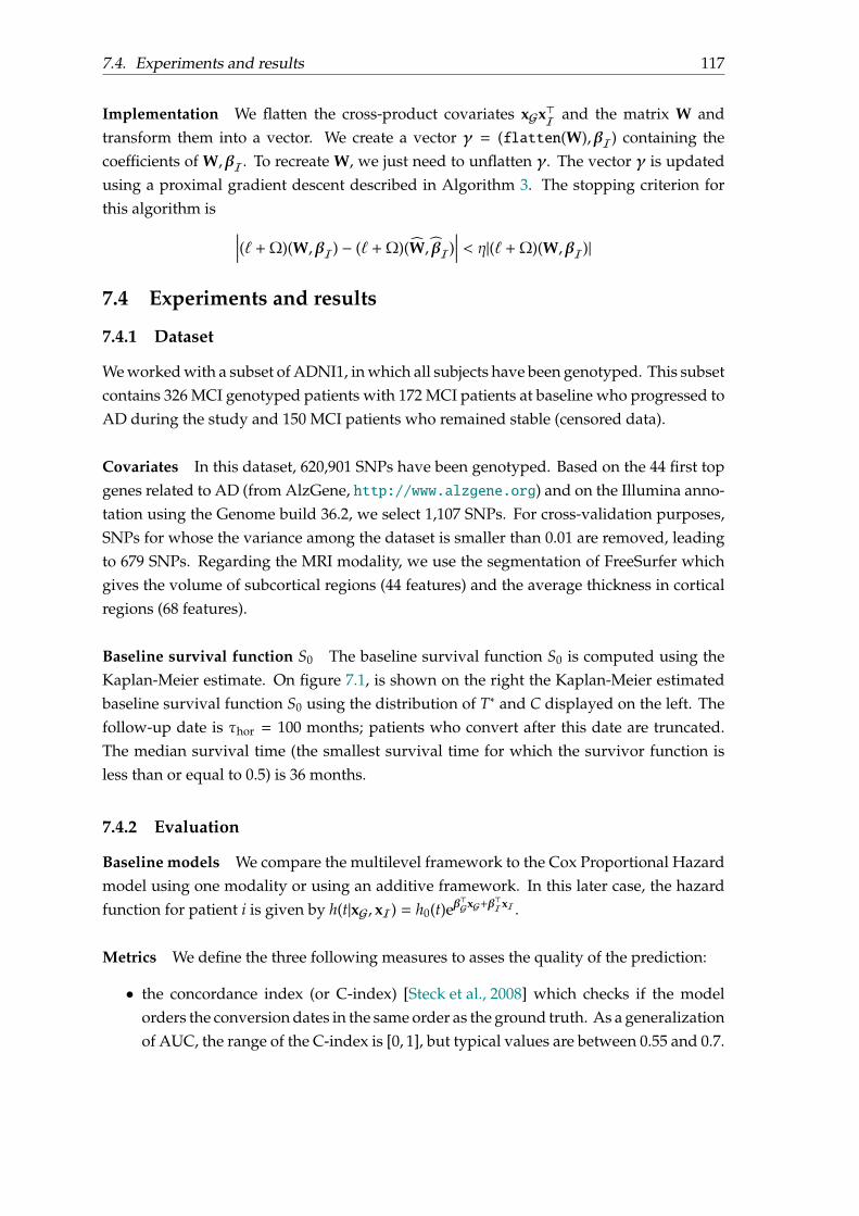
7.4. Experiments and results 117

Implementation We flatten the cross-product covariates xGx⊤I and the matrix W andtransform them into a vector. We create a vector γ = (flatten(W),βI) containing thecoefficients of W,βI. To recreate W, we just need to unflatten γ. The vector γ is updatedusing a proximal gradient descent described in Algorithm 3. The stopping criterion forthis algorithm is ∣∣∣∣(ℓ +Ω)(W,βI) − (ℓ +Ω)(W, βI)

∣∣∣∣ < η|(ℓ +Ω)(W,βI)|

7.4 Experiments and results

7.4.1 Dataset

We worked with a subset of ADNI1, in which all subjects have been genotyped. This subsetcontains 326 MCI genotyped patients with 172 MCI patients at baseline who progressed toAD during the study and 150 MCI patients who remained stable (censored data).

Covariates In this dataset, 620,901 SNPs have been genotyped. Based on the 44 first topgenes related to AD (from AlzGene, http://www.alzgene.org) and on the Illumina anno-tation using the Genome build 36.2, we select 1,107 SNPs. For cross-validation purposes,SNPs for whose the variance among the dataset is smaller than 0.01 are removed, leadingto 679 SNPs. Regarding the MRI modality, we use the segmentation of FreeSurfer whichgives the volume of subcortical regions (44 features) and the average thickness in corticalregions (68 features).

Baseline survival function S0 The baseline survival function S0 is computed using theKaplan-Meier estimate. On figure 7.1, is shown on the right the Kaplan-Meier estimatedbaseline survival function S0 using the distribution of T∗ and C displayed on the left. Thefollow-up date is τhor = 100 months; patients who convert after this date are truncated.The median survival time (the smallest survival time for which the survivor function isless than or equal to 0.5) is 36 months.

7.4.2 Evaluation

Baseline models We compare the multilevel framework to the Cox Proportional Hazardmodel using one modality or using an additive framework. In this later case, the hazardfunction for patient i is given by h(t|xG, xI) = h0(t)eβ

⊤GxG+β⊤IxI .

Metrics We define the three following measures to asses the quality of the prediction:

• the concordance index (or C-index) [Steck et al., 2008] which checks if the modelorders the conversion dates in the same order as the ground truth. As a generalizationof AUC, the range of the C-index is [0, 1], but typical values are between 0.55 and 0.7.

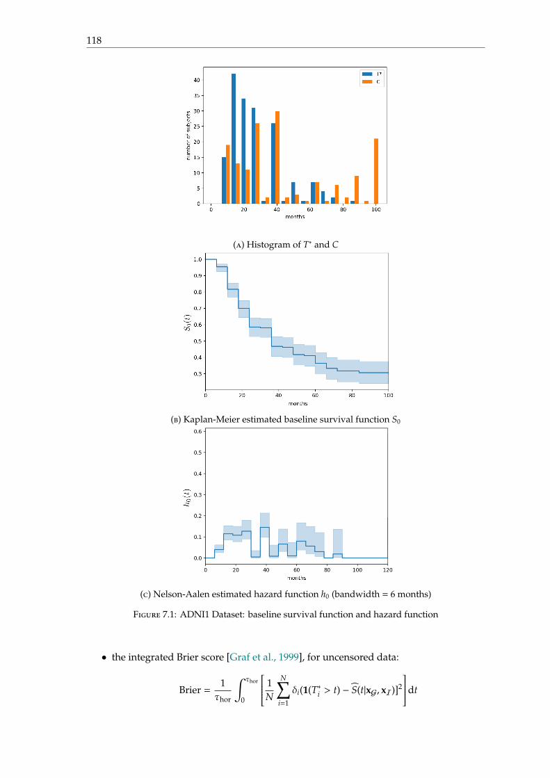
118

(a) Histogram of T∗ and C

(b) Kaplan-Meier estimated baseline survival function S0

(c) Nelson-Aalen estimated hazard function h0 (bandwidth = 6 months)

Figure 7.1: ADNI1 Dataset: baseline survival function and hazard function

• the integrated Brier score [Graf et al., 1999], for uncensored data:

Brier =1τhor

∫ τhor

0

1N

N∑i=1

δi(1(T∗i > t) − S(t|xG, xI)]2

dt

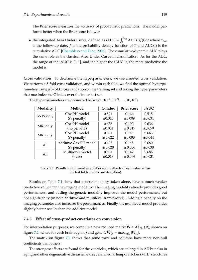
7.4. Experiments and results 119

The Brier score measures the accuracy of probabilistic predictions. The model per-forms better when the Brier score is lower.

• the integrated Area Under Curve, defined as iAUC =∫ τhor

0 AUC(t) f (t)dt where τhor

is the follow-up date, f is the probability density function of T and AUC(t) is thecumulative AUC [Chambless and Diao, 2006]. The cumulative/dynamic AUC playsthe same role as the classical Area Under Curve in classification. As for the AUC,the range of the iAUC is [0, 1], and the higher the iAUC is, the more predictive themodel is.

Cross validation To determine the hyperparameters, we use a nested cross validation.We perform a 5-fold cross validation, and within each fold, we find the optimal hyperpa-rameters using a 5-fold cross validation on the training set and taking the hyperparametersthat maximize the C-index over the inner test set.

The hyperparameters are optimized between 10−4, 10−3, . . . , 10, 102.

Modality Method C-index Brier score iAUC

SNPs onlyCox PH model 0.521 0.166 0.515

(ℓ1 penalty) ±0.040 ±0.009 ±0.031

MRI onlyCox PH model 0.636 0.190 0.636

(no penalty) ±0.034 ± 0.017 ±0.050

MRI onlyCox PH model 0.671 0.149 0.663

(ℓ2 penalty) ± 0.022 ±0.008 ±0.044

AllAdditive Cox PH model 0.677 0.148 0.680

(ℓ1 penalty) ± 0.020 ± 0.006 ±0.030

AllMultilevel model 0.681 0.147 0.686

(ours) ±0.018 ± 0.006 ±0.031

Table 7.1: Results for different modalities and methods (mean value acrossthe test folds ± standard deviation)

Results on Table 7.1 show that genetic modality, taken alone, have a much weakerpredictive value than the imaging modality. The imaging modality already provides goodperformances, and adding the genetic modality improves the model performance, butnot significantly (in both additive and multilevel frameworks). Adding a penalty on theimaging parameter also increases the performances. Finally, the multilevel model providesslightly better results than the additive model.

7.4.3 Effect of cross-product covariates on conversion

For interpretation purposes, we compute a new reduced matrix W ∈ M|I|,L(R), shown onfigure 7.2, where for each brain region j and gene ℓ, W j,ℓ = maxs∈Gℓ |Ws, j|.

The matrix on figure 7.2 shows that some rows and columns have more non-nullcoefficients than others.

The strongest effects are found for the ventricles, which are enlarged in AD but also inaging and other degenerative diseases, and several medial temporal lobes (MTL) structures

120

(entorhinal cortex, hippocampus, amygdala) which are altered early in AD. It is interestingto note that the ventricles have a strong interaction with all genes except APOE, whilethe MTL structures have interactions with a more restricted but quite consistent set ofgenes. Regarding the genes, the strongest effects are found for the single-nucleotidepolymorphism rs6503018 (TNK1), rs429358 (APOE) and rs3093662 (TNF).

7.5 Conclusion

We proposed a novel approach to estimate the conversion date to AD for MCI patients,using the Cox Proportional Hazard model, from genetic and neuroimaging data. On thecontrary of additive models, the multilevel model captures interactions between genesand brain regions. The use of adapted penalties avoids overfitting by providing a sparsematrix and highlighting brain regions and genes both related to the progression to AD.

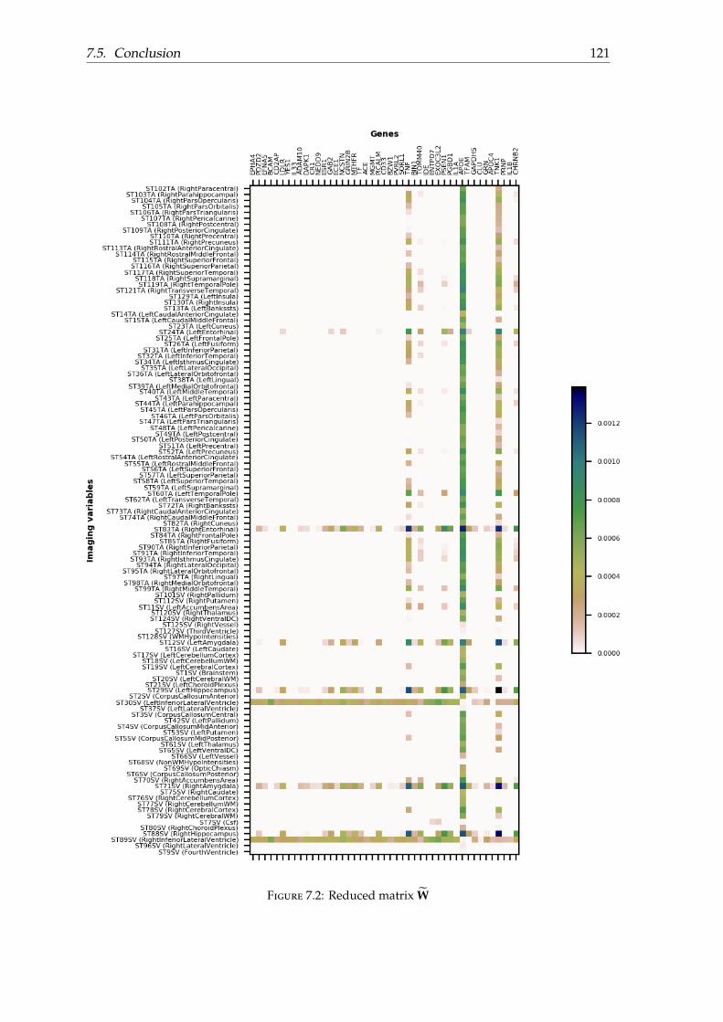
7.5. Conclusion 121

Figure 7.2: Reduced matrix W

123

Conclusion

In this PhD, we have explored the idea that modalities from different sources, instead ofbeing simply added together in an additive model, could be multiplied using a multilevelframework in order to capture interactions between modalities. A multilevel frameworkwill allow to hierarchise modalities and to use different level of decisions. In chapter 4, weproposed a multilevel classification framework for the diagnosis of Alzheimer’s Disease.As we worked with high-dimensional data, we used adapted penalties for each modalityand their joint interactions. In addition to providing a moderately higher predictive power,this approach is able to capture potential interactions between the genetic covariates, thebrain regions, and their relation to the disease. The model uses both genetic and neu-roimaging data together in order for assisting diagnosis, but also relates genetic covariatesand brain regions as in an association study in imaging genetics.

Then, we focused on the prediction of the conversion date to Alzheimer’s Disease.This question has recently become a major interest of the community. In particular, it wasthe objective of the TADPOLE challenge launched in 2017. We proposed a contributionto this challenge using a standard survival model, namely Aalen’s additive model. Thiscontribution ranked high on one of the outcomes of the challenge. Surprisingly, wewere one of the only teams to use a survival model, even though this approach is wellsuited to the problem. We believe that it is due to the fact that such models, whileclassical in the statistics community, are less well known in the medical image analysisand machine learning communities. The interest of survival approaches were confirmedby experiments done in chapter 6 which showed that doing a classification at repeatedfixed times and using some basic survival models provide similar results in terms of areaunder the ROC curve, but survival models as a whole are slightly better when it comesto consider the balanced classification accuracy. We then proposed several extensionsof survival analysis to multimodal data. We first tried to extend the log-logistic survivalmodel, by setting a speed and a position that depend on clinical and genetic data. However,results showed that this log-logistic model tended to be biased and resulted in lowerperformance compared to basic survival approaches. Then in chapter 7, we proposed aCox multiplicative survival model which extends the approach of Chapter 4 to survivalanalysis. The performance was slightly higher than that of an additive Cox model. Moreinterestingly, as in Chapter 4, our method allowed revealing interactions between imagingand genetic data.

Future work

There are multiple perspectives to this work.

124

First, the proposed multilevel methodology for combining genetic covariates andanatomical brain regions can be applied to other modalities, for instance using the PETneuroimaging modality and/or clinical scores. From a practical point of view, this hasthe potential to increase the classification accuracy. Indeed, recent papers have reportedthat PET is superior to MRI for AD classification [Samper-González et al., 2018] and thatthe combination of clinical and imaging data is superior to imaging alone for predictingprogression to AD [Samper-Gonzalez et al., 2019].

In the present manuscript, the results of the TADPOLE challenge concern predictionat one year. Indeed, the evaluation is based on the future visits in the ADNI study whichbecome available progressively. Thus, evaluations will continue every year until 2022. Itwill be interesting to continue to observe the ranking of the proposed method comparedto other submissions.

During our experiments, we noticed a clear relationship, in terms of variations andsigns, between the parameter coefficients of a fixed-time logistic regression and of theAalen additive model. Although these parameter coefficients of both model are not learntin the same way, as the logistic regression does not use temporal information, whereas theAalen additive model. It can be interesting to focus on a theoretical relation between bothmodels.

Using other datasets on Alzheimer’s Disease (that provide genetic data and clinicaldata) would have been interesting. First, it would be interesting to check if all the previousmodels have the same behaviour on different datasets and how well they would generaliseacross datasets. More specifically, it would be interesting to see if the log-logistic model isstill biased.

Finally, in our work, we did not consider death as a competing risk with Alzheimer’sDisease. It could be interesting to take it into account. This could be done using the frame-work of multistate survival models. More generally, we could consider other competingrisks such as other forms of dementia or even other diseases. This could pave the way tomore general predictive models.

125

Appendix

127

Scientific production

Journal papers

• Samper-Gonzalez Jorge, Burgos Ninon, Bottani Simona, Fontanella Sabrina, Lu Pas-cal, Marcoux Arnaud, Routier Alexandre, Guillon Jérémy, Bacci Michael, Wen Jun-hao, Bertrand Anne, Bertin Hugo, Habert Marie-Odile, Durrleman Stanley, EvgeniouTheodoros, and Colliot Olivier, for the ADNI & the AIBL, Reproducible evaluationof classification methods in Alzheimers disease: Framework and application to MRIand PET data, NeuroImage, 183, 504521, 2018. https://hal.inria.fr/hal-01858384

Conference papers

• Lu Pascal, Colliot Olivier. Multilevel Modeling with Structured Penalties for Clas-sification from Imaging Genetics data. 3rd MICCAI Workshop on Imaging Genetics(MICGen 2017), Sep 2017, Quebec City, Canada. pp.230-240.

• Lu Pascal, Colliot Olivier. Multilevel Survival Analysis with Structured Penalties forImaging Genetics data. Accepted at SPIE 2020 Medical Imaging.

Posters and talks

• Lu Pascal, Colliot Olivier. Multilevel Survival Analysis with Structured Penalties forImaging Genetics data. Poster at GDR Statistiques & Santé, Paris, October 2019.

• Lu Pascal, Colliot Olivier. A log-logistic survival model from multimodal data forprediction of Alzheimer’s Disease. Poster at SAFJR 2019, Copenhagen, April 2019.

• Lu Pascal, Colliot Olivier. Multilevel Modeling with Structured Penalties for Classi-fication from Imaging Genetics data. Poster at ICM - IoN Workshop, London, UK,October 2017.

• Lu Pascal, Colliot Olivier. Multilevel Modeling with Structured Penalties for Clas-sification from Imaging Genetics data. Oral presentation at MICGen 2017, Quebec,Canada, September 2017.

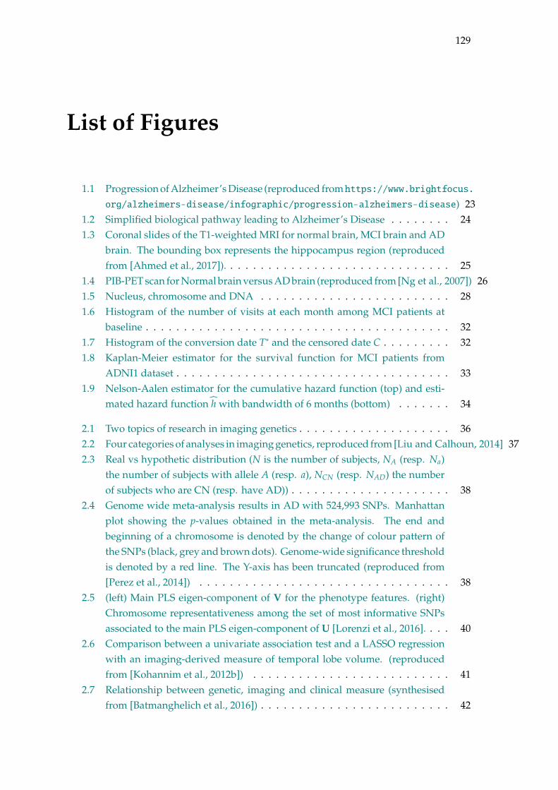
129

List of Figures

1.1 Progression of Alzheimer’s Disease (reproduced fromhttps://www.brightfocus.org/alzheimers-disease/infographic/progression-alzheimers-disease) 23

1.2 Simplified biological pathway leading to Alzheimer’s Disease . . . . . . . . 241.3 Coronal slides of the T1-weighted MRI for normal brain, MCI brain and AD

brain. The bounding box represents the hippocampus region (reproducedfrom [Ahmed et al., 2017]). . . . . . . . . . . . . . . . . . . . . . . . . . . . . . 25

1.4 PIB-PET scan for Normal brain versus AD brain (reproduced from [Ng et al., 2007]) 261.5 Nucleus, chromosome and DNA . . . . . . . . . . . . . . . . . . . . . . . . . 281.6 Histogram of the number of visits at each month among MCI patients at

baseline . . . . . . . . . . . . . . . . . . . . . . . . . . . . . . . . . . . . . . . . 321.7 Histogram of the conversion date T∗ and the censored date C . . . . . . . . . 321.8 Kaplan-Meier estimator for the survival function for MCI patients from

ADNI1 dataset . . . . . . . . . . . . . . . . . . . . . . . . . . . . . . . . . . . . 331.9 Nelson-Aalen estimator for the cumulative hazard function (top) and esti-

mated hazard function h with bandwidth of 6 months (bottom) . . . . . . . 34

2.1 Two topics of research in imaging genetics . . . . . . . . . . . . . . . . . . . . 362.2 Four categories of analyses in imaging genetics, reproduced from [Liu and Calhoun, 2014] 372.3 Real vs hypothetic distribution (N is the number of subjects, NA (resp. Na)

the number of subjects with allele A (resp. a), NCN (resp. NAD) the numberof subjects who are CN (resp. have AD)) . . . . . . . . . . . . . . . . . . . . . 38

2.4 Genome wide meta-analysis results in AD with 524,993 SNPs. Manhattanplot showing the p-values obtained in the meta-analysis. The end andbeginning of a chromosome is denoted by the change of colour pattern ofthe SNPs (black, grey and brown dots). Genome-wide significance thresholdis denoted by a red line. The Y-axis has been truncated (reproduced from[Perez et al., 2014]) . . . . . . . . . . . . . . . . . . . . . . . . . . . . . . . . . 38

2.5 (left) Main PLS eigen-component of V for the phenotype features. (right)Chromosome representativeness among the set of most informative SNPsassociated to the main PLS eigen-component of U [Lorenzi et al., 2016]. . . . 40

2.6 Comparison between a univariate association test and a LASSO regressionwith an imaging-derived measure of temporal lobe volume. (reproducedfrom [Kohannim et al., 2012b]) . . . . . . . . . . . . . . . . . . . . . . . . . . 41

2.7 Relationship between genetic, imaging and clinical measure (synthesisedfrom [Batmanghelich et al., 2016]) . . . . . . . . . . . . . . . . . . . . . . . . . 42

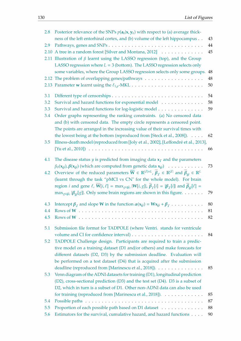
130 List of Figures

2.8 Posterior relevance of the SNPs p(ak|x,yk) with respect to (a) average thick-ness of the left entorhinal cortex, and (b) volume of the left hippocampus . . 43

2.9 Pathways, genes and SNPs . . . . . . . . . . . . . . . . . . . . . . . . . . . . . 442.10 A tree in a random forest [Silver and Montana, 2012] . . . . . . . . . . . . . 452.11 Illustration of β learnt using the LASSO regression (top), and the Group

LASSO regression where L = 3 (bottom). The LASSO regression selects onlysome variables, where the Group LASSO regression selects only some groups. 48

2.12 The problem of overlapping genes/pathways . . . . . . . . . . . . . . . . . . 482.13 Parameter w learnt using the ℓ1,p-MKL . . . . . . . . . . . . . . . . . . . . . . 50

3.1 Different type of censorships . . . . . . . . . . . . . . . . . . . . . . . . . . . . 543.2 Survival and hazard functions for exponential model . . . . . . . . . . . . . 583.3 Survival and hazard functions for log-logistic model . . . . . . . . . . . . . . 593.4 Order graphs representing the ranking constraints. (a) No censored data

and (b) with censored data. The empty circle represents a censored point.The points are arranged in the increasing value of their survival times withthe lowest being at the bottom (reproduced from [Steck et al., 2008]). . . . . 62

3.5 Illness-death model (reproduced from [Joly et al., 2002], [Leffondré et al., 2013],[Yu et al., 2010]) . . . . . . . . . . . . . . . . . . . . . . . . . . . . . . . . . . . 66

4.1 The disease status y is predicted from imaging data xI and the parametersβ0(xG),β(xG) (which are computed from genetic data xG) . . . . . . . . . . . 73

4.2 Overview of the reduced parameters W ∈ R|I|×L, βI ∈ R|I| and βG ∈ RL

(learnt through the task “pMCI vs CN" for the whole model). For brainregion i and gene ℓ, W[i, ℓ] = maxg∈Gℓ |W[i, g]|, βI[i] = |βI[i]| and βG[ℓ] =maxg∈Gℓ |βG[g]|. Only some brain regions are shown in this figure. . . . . . . 79

4.3 Intercept βI and slope W in the function α(xG) =WxG + βI . . . . . . . . . . 804.4 Rows of W . . . . . . . . . . . . . . . . . . . . . . . . . . . . . . . . . . . . . . 814.5 Rows of W . . . . . . . . . . . . . . . . . . . . . . . . . . . . . . . . . . . . . . 82

5.1 Submission file format for TADPOLE (where Ventri. stands for ventriculevolume and CI for confidence interval) . . . . . . . . . . . . . . . . . . . . . . 84

5.2 TADPOLE Challenge design. Participants are required to train a predic-tive model on a training dataset (D1 and/or others) and make forecasts fordifferent datasets (D2, D3) by the submission deadline. Evaluation willbe performed on a test dataset (D4) that is acquired after the submissiondeadline (reproduced from [Marinescu et al., 2018]). . . . . . . . . . . . . . . 85

5.3 Venn diagram of the ADNI datasets for training (D1), longitudinal prediction(D2), cross-sectional prediction (D3) and the test set (D4). D3 is a subset ofD2, which in turn is a subset of D1. Other non-ADNI data can also be usedfor training (reproduced from [Marinescu et al., 2018]). . . . . . . . . . . . . 85

5.4 Possible paths . . . . . . . . . . . . . . . . . . . . . . . . . . . . . . . . . . . . 875.5 Proportion of each possible path based on D1 dataset . . . . . . . . . . . . . 885.6 Estimators for the survival, cumulative hazard, and hazard functions . . . . 90

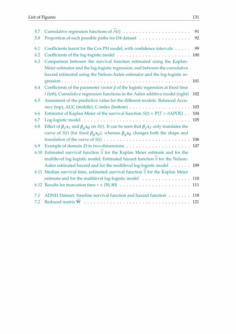
List of Figures 131

5.7 Cumulative regression functions of A(t) . . . . . . . . . . . . . . . . . . . . . 915.8 Proportion of each possible paths for D4 dataset . . . . . . . . . . . . . . . . 92

6.1 Coefficients learnt for the Cox PH model, with confidence intervals . . . . . 996.2 Coefficients of the log-logistic model . . . . . . . . . . . . . . . . . . . . . . . 1006.3 Comparison between the survival function estimated using the Kaplan-

Meier estimator and the log-logistic regression; and between the cumulativehazard estimated using the Nelson-Aalen estimator and the log-logistic re-gression . . . . . . . . . . . . . . . . . . . . . . . . . . . . . . . . . . . . . . . . 101

6.4 Coefficients of the parameter vector β of the logistic regression at fixed timet (left); Cumulative regression functions in the Aalen additive model (right) 102

6.5 Assesment of the predictive value for the different models: Balanced Accu-racy (top), AUC (middle), C-index (bottom) . . . . . . . . . . . . . . . . . . . 103

6.6 Estimator of Kaplan-Meier of the survival function S(t) = PT > t|APOE . . 1046.7 Log-logistic model . . . . . . . . . . . . . . . . . . . . . . . . . . . . . . . . . 1056.8 Effect of βIxI and βGxG on S(t). It can be seen that βIxI only translates the

curve of S(t) (for fixed βGxG), whereas βGxG changes both the shape andtranslation of the curve of S(t) . . . . . . . . . . . . . . . . . . . . . . . . . . . 106

6.9 Example of domainD in two-dimensions . . . . . . . . . . . . . . . . . . . . 1076.10 Estimated survival function S for the Kaplan Meier estimate and for the

multilevel log-logistic model; Estimated hazard function h for the Nelson-Aalen estimated hazard and for the multilevel log-logistic model . . . . . . 109

6.11 Median survival time, estimated survival function S for the Kaplan Meierestimate and for the multilevel log-logistic model . . . . . . . . . . . . . . . 110

6.12 Results for truncation time τ ∈ 50, 80 . . . . . . . . . . . . . . . . . . . . . . 111

7.1 ADNI1 Dataset: baseline survival function and hazard function . . . . . . . 1187.2 Reduced matrix W . . . . . . . . . . . . . . . . . . . . . . . . . . . . . . . . . 121

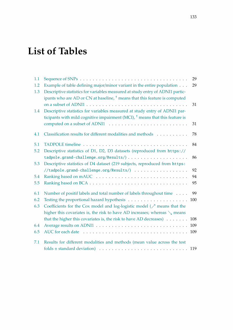
133

List of Tables

1.1 Sequence of SNPs . . . . . . . . . . . . . . . . . . . . . . . . . . . . . . . . . . 291.2 Example of table defining major/minor variant in the entire population . . . 291.3 Descriptive statistics for variables measured at study entry of ADNI1 partic-

ipants who are AD or CN at baseline, † means that this feature is computedon a subset of ADNI1 . . . . . . . . . . . . . . . . . . . . . . . . . . . . . . . . 31

1.4 Descriptive statistics for variables measured at study entry of ADNI1 par-ticipants with mild cognitive impairment (MCI), † means that this feature iscomputed on a subset of ADNI1 . . . . . . . . . . . . . . . . . . . . . . . . . 31

4.1 Classification results for different modalities and methods . . . . . . . . . . 78

5.1 TADPOLE timeline . . . . . . . . . . . . . . . . . . . . . . . . . . . . . . . . . 845.2 Descriptive statistics of D1, D2, D3 datasets (reproduced from https://

tadpole.grand-challenge.org/Results/) . . . . . . . . . . . . . . . . . . . 865.3 Descriptive statistics of D4 dataset (219 subjects, reproduced from https:

//tadpole.grand-challenge.org/Results/) . . . . . . . . . . . . . . . . . 925.4 Ranking based on mAUC . . . . . . . . . . . . . . . . . . . . . . . . . . . . . 945.5 Ranking based on BCA . . . . . . . . . . . . . . . . . . . . . . . . . . . . . . . 95

6.1 Number of positif labels and total number of labels throughout time . . . . 996.2 Testing the proportional hazard hypothesis . . . . . . . . . . . . . . . . . . . 1006.3 Coefficients for the Cox model and log-logistic model ( means that the

higher this covariates is, the risk to have AD increases; whereas meansthat the higher this covariates is, the risk to have AD decreases) . . . . . . . 108

6.4 Average results on ADNI1 . . . . . . . . . . . . . . . . . . . . . . . . . . . . . 1096.5 AUC for each date . . . . . . . . . . . . . . . . . . . . . . . . . . . . . . . . . 109

7.1 Results for different modalities and methods (mean value across the testfolds ± standard deviation) . . . . . . . . . . . . . . . . . . . . . . . . . . . . 119

135

Bibliography

[Aalen, 1980] Aalen, O. (1980). A Model for Nonparametric Regression Analysis of Count-ing Processes. In Klonecki, W., Kozek, A., and Rosiski, J., editors, Mathematical Statisticsand Probability Theory, Lecture Notes in Statistics, pages 1–25, New York, NY. Springer.

[Ahmed et al., 2017] Ahmed, O. B., Benois-Pineau, J., Allard, M., Catheline, G., and Amar,C. B. (2017). Recognition of Alzheimer’s disease and Mild Cognitive Impairment withmultimodal image-derived biomarkers and Multiple Kernel Learning. Neurocomputing,220:98–110.

[Aiolli and Donini, 2015] Aiolli, F. and Donini, M. (2015). EasyMKL: a scalable multiplekernel learning algorithm. Neurocomputing, 169:215–224.

[Anderson et al., 2016] Anderson, E. D., Wahoske, M., Huber, M., Norton, D., Li, Z.,Koscik, R. L., Umucu, E., Johnson, S. C., Jones, J., Asthana, S., and Gleason, C. E.(2016). Cognitive variabilityA marker for incident MCI and AD: An analysis for theAlzheimer’s Disease Neuroimaging Initiative. Alzheimer’s & Dementia: Diagnosis, As-sessment & Disease Monitoring, 4:47–55.

[Batmanghelich et al., 2016] Batmanghelich, N. K., Dalca, A., Quon, G., Sabuncu, M., andGolland, P. (2016). Probabilistic Modeling of Imaging, Genetics and Diagnosis. IEEETransactions on Medical Imaging, 35(7):1765–1779.

[Beck and Teboulle, 2009] Beck, A. and Teboulle, M. (2009). Gradient-based algorithmswith applications to signal-recovery problems.

[Binder and Schumacher, 2016] Binder, N. and Schumacher, M. (2016). Incidence of De-mentia over Three Decades in the Framingham Heart Study. New England Journal ofMedicine, 375(1):92–94.

[Bøvelstad et al., 2009] Bøvelstad, H. M., Nygård, S., and Borgan, . (2009). Survival predic-tion from clinico-genomic models - a comparative study. BMC Bioinformatics, 10(1):413.

[Chambless and Diao, 2006] Chambless, L. E. and Diao, G. (2006). Estimation of time-dependent area under the ROC curve for long-term risk prediction. Statistics in Medicine,25(20):3474–3486.

[Chekouo et al., 2016] Chekouo, T., Stingo, F. C., Guindani, M., and Do, K.-A. (2016). ABayesian predictive model for imaging genetics with application to schizophrenia. TheAnnals of Applied Statistics, 10(3):1547–1571.

136 BIBLIOGRAPHY

[Cheng et al., 2015] Cheng, B., Liu, M., Zhang, D., Munsell, B. C., and Shen, D. (2015).Domain Transfer Learning for MCI Conversion Prediction. IEEE transactions on bio-medical engineering, 62(7):1805–1817.

[Davatzikos et al., 2011] Davatzikos, C., Bhatt, P., Shaw, L. M., Batmanghelich, K. N., andTrojanowski, J. Q. (2011). Prediction of MCI to AD conversion, via MRI, CSF biomarkers,and pattern classification. Neurobiology of Aging, 32(12):2322.e19–27.

[Du et al., 2014] Du, L., Jingwen, Y., Kim, S., Risacher, S. L., Huang, H., Inlow, M., Moore,J. H., Saykin, A. J., Shen, L., and Alzheimer’s Disease Neuroimaging Initiative (2014).A novel structure-aware sparse learning algorithm for brain imaging genetics. Medicalimage computing and computer-assisted intervention: MICCAI ... International Conference onMedical Image Computing and Computer-Assisted Intervention, 17(Pt 3):329–336.

[Dubois and Albert, 2004] Dubois, B. and Albert, M. L. (2004). Amnestic MCI or prodromalAlzheimer’s disease? The Lancet Neurology, 3(4):246–248.

[Dubois et al., 2007] Dubois, B., Feldman, H. H., Jacova, C., Dekosky, S. T., Barberger-Gateau, P., Cummings, J., Delacourte, A., Galasko, D., Gauthier, S., Jicha, G., Meguro,K., O’brien, J., Pasquier, F., Robert, P., Rossor, M., Salloway, S., Stern, Y., Visser, P. J., andScheltens, P. (2007). Research criteria for the diagnosis of Alzheimer’s disease: revisingthe NINCDS-ADRDA criteria. The Lancet. Neurology, 6(8):734–746.

[Dubois et al., 2014] Dubois, B., Feldman, H. H., Jacova, C., Hampel, H., Molinuevo, J. L.,Blennow, K., DeKosky, S. T., Gauthier, S., Selkoe, D., Bateman, R., Cappa, S., Crutch,S., Engelborghs, S., Frisoni, G. B., Fox, N. C., Galasko, D., Habert, M.-O., Jicha, G. A.,Nordberg, A., Pasquier, F., Rabinovici, G., Robert, P., Rowe, C., Salloway, S., Sarazin, M.,Epelbaum, S., de Souza, L. C., Vellas, B., Visser, P. J., Schneider, L., Stern, Y., Scheltens,P., and Cummings, J. L. (2014). Advancing research diagnostic criteria for Alzheimer’sdisease: the IWG-2 criteria. The Lancet. Neurology, 13(6):614–629.

[Dubois et al., 2016] Dubois, B., Hampel, H., Feldman, H. H., Scheltens, P., Aisen, P., An-drieu, S., Bakardjian, H., Benali, H., Bertram, L., Blennow, K., Broich, K., Cavedo, E.,Crutch, S., Dartigues, J.-F., Duyckaerts, C., Epelbaum, S., Frisoni, G. B., Gauthier, S.,Genthon, R., Gouw, A. A., Habert, M.-O., Holtzman, D. M., Kivipelto, M., Lista, S.,Molinuevo, J.-L., O’Bryant, S. E., Rabinovici, G. D., Rowe, C., Salloway, S., Schnei-der, L. S., Sperling, R., Teichmann, M., Carrillo, M. C., Cummings, J., and Jack, C. R.(2016). Preclinical Alzheimer’s disease: Definition, natural history, and diagnostic crite-ria. Alzheimer’s & Dementia: The Journal of the Alzheimer’s Association, 12(3):292–323.

[Duyckaerts et al., 2009] Duyckaerts, C., Delatour, B., and Potier, M.-C. (2009). Classifica-tion and basic pathology of Alzheimer disease. Acta Neuropathologica, 118(1):5–36.

[Graf et al., 1999] Graf, E., Schmoor, C., Sauerbrei, W., and Schumacher, M. (1999). Assess-ment and comparison of prognostic classification schemes for survival data. Statistics inMedicine, 18(17-18):2529–2545.

BIBLIOGRAPHY 137

[Gönen and Alpaydn, 2011] Gönen, M. and Alpaydn, E. (2011). Multiple Kernel LearningAlgorithms. Journal of Machine Learning Research, 12(Jul):2211–2268.

[Hampel et al., 2014] Hampel, H., Lista, S., Teipel, S. J., Garaci, F., Nisticò, R., Blennow,K., Zetterberg, H., Bertram, L., Duyckaerts, C., Bakardjian, H., Drzezga, A., Colliot, O.,Epelbaum, S., Broich, K., Lehéricy, S., Brice, A., Khachaturian, Z. S., Aisen, P. S., andDubois, B. (2014). Perspective on future role of biological markers in clinical therapytrials of Alzheimer’s disease: a long-range point of view beyond 2020. BiochemicalPharmacology, 88(4):426–449.

[Hastie et al., 2015] Hastie, T., Tibshirani, R., and Wainwright, M. (2015). Statistical Learningwith Sparsity - The Lasso and Generalizations, volume 143 of Monographs on Statistics andApplied Probability 143. Crc press edition.

[Jacob et al., 2009] Jacob, L., Obozinski, G., and Vert, J.-P. (2009). Group Lasso with Overlapand Graph Lasso. Proceedings of the 26 th International Conference on Machine Learning.

[Janssen et al., 2000] Janssen, J. C., Hall, M., Fox, N. C., Harvey, R. J., Beck, J., Dickinson,A., Campbell, T., Collinge, J., Lantos, P. L., Cipolotti, L., Stevens, J. M., and Rossor, M. N.(2000). Alzheimer’s disease due to an intronic presenilin-1 (PSEN1 intron 4) mutationAclinicopathological study. Brain, 123(5):894–907.

[Joly et al., 2002] Joly, P., Commenges, D., Helmer, C., and Letenneur, L. (2002). A penal-ized likelihood approach for an illness-death model with interval-censored data: appli-cation to age-specific incidence of dementia. Biostatistics (Oxford, England), 3(3):433–443.

[Kloft et al., 2011] Kloft, M., Brefeld, U., Sonnenburg, S., and Zien, A. (2011). lp-NormMultiple Kernel Learning. Journal of Machine Learning Research, 12(Mar):953–997.

[Kohannim et al., 2012a] Kohannim, O., Hibar, D. P., Stein, J. L., Jahanshad, N., Hua, X.,Rajagopalan, P., Toga, A. W., Jack, C. R., Weiner, M. W., de Zubicaray, G. I., McMahon,K. L., Hansell, N. K., Martin, N. G., Wright, M. J., Thompson, P. M., and AlzheimersDisease Neuroimaging Initiative (2012a). Discovery and Replication of Gene Influenceson Brain Structure Using LASSO Regression. Frontiers in Neuroscience, 6:115.

[Kohannim et al., 2012b] Kohannim, O., Hibar, D. P., Stein, J. L., Jahanshad, N., Hua, X.,Rajagopalan, P., Toga, A. W., Jack, C. R., Weiner, M. W., de Zubicaray, G. I., McMahon,K. L., Hansell, N. K., Martin, N. G., Wright, M. J., Thompson, P. M., and AlzheimersDisease Neuroimaging Initiative (2012b). Discovery and Replication of Gene Influenceson Brain Structure Using LASSO Regression. Frontiers in Neuroscience, 6:115.

[Laird and Lange, 2011] Laird, N. M. and Lange, C. (2011). Introduction to StatisticalGenetics and Background in Molecular Genetics. In The Fundamentals of Modern StatisticalGenetics, Statistics for Biology and Health, pages 1–13. Springer New York.

[Lambert et al., 2013] Lambert, J. C., Ibrahim-Verbaas, C. A., Harold, D., Naj, A. C., Sims,R., Bellenguez, C., DeStafano, A. L., Bis, J. C., Beecham, G. W., Grenier-Boley, B., Russo,G., Thorton-Wells, T. A., Jones, N., Smith, A. V., Chouraki, V., Thomas, C., Ikram,

138 BIBLIOGRAPHY

M. A., Zelenika, D., Vardarajan, B. N., Kamatani, Y., Lin, C. F., Gerrish, A., Schmidt, H.,Kunkle, B., Dunstan, M. L., Ruiz, A., Bihoreau, M. T., Choi, S. H., Reitz, C., Pasquier, F.,Cruchaga, C., Craig, D., Amin, N., Berr, C., Lopez, O. L., De Jager, P. L., Deramecourt,V., Johnston, J. A., Evans, D., Lovestone, S., Letenneur, L., Morón, F. J., Rubinsztein,D. C., Eiriksdottir, G., Sleegers, K., Goate, A. M., Fiévet, N., Huentelman, M. W., Gill,M., Brown, K., Kamboh, M. I., Keller, L., Barberger-Gateau, P., McGuiness, B., Larson,E. B., Green, R., Myers, A. J., Dufouil, C., Todd, S., Wallon, D., Love, S., Rogaeva, E.,Gallacher, J., St George-Hyslop, P., Clarimon, J., Lleo, A., Bayer, A., Tsuang, D. W.,Yu, L., Tsolaki, M., Bossù, P., Spalletta, G., Proitsi, P., Collinge, J., Sorbi, S., Sanchez-Garcia, F., Fox, N. C., Hardy, J., Deniz Naranjo, M. C., Bosco, P., Clarke, R., Brayne,C., Galimberti, D., Mancuso, M., Matthews, F., European Alzheimer’s Disease Initiative(EADI), Genetic and Environmental Risk in Alzheimer’s Disease, Alzheimer’s DiseaseGenetic Consortium, Cohorts for Heart and Aging Research in Genomic Epidemiology,Moebus, S., Mecocci, P., Del Zompo, M., Maier, W., Hampel, H., Pilotto, A., Bullido, M.,Panza, F., Caffarra, P., Nacmias, B., Gilbert, J. R., Mayhaus, M., Lannefelt, L., Hakonarson,H., Pichler, S., Carrasquillo, M. M., Ingelsson, M., Beekly, D., Alvarez, V., Zou, F.,Valladares, O., Younkin, S. G., Coto, E., Hamilton-Nelson, K. L., Gu, W., Razquin, C.,Pastor, P., Mateo, I., Owen, M. J., Faber, K. M., Jonsson, P. V., Combarros, O., O’Donovan,M. C., Cantwell, L. B., Soininen, H., Blacker, D., Mead, S., Mosley, T. H., Bennett, D. A.,Harris, T. B., Fratiglioni, L., Holmes, C., de Bruijn, R. F., Passmore, P., Montine, T. J.,Bettens, K., Rotter, J. I., Brice, A., Morgan, K., Foroud, T. M., Kukull, W. A., Hannequin,D., Powell, J. F., Nalls, M. A., Ritchie, K., Lunetta, K. L., Kauwe, J. S., Boerwinkle, E.,Riemenschneider, M., Boada, M., Hiltuenen, M., Martin, E. R., Schmidt, R., Rujescu, D.,Wang, L. S., Dartigues, J. F., Mayeux, R., Tzourio, C., Hofman, A., Nöthen, M. M., Graff,C., Psaty, B. M., Jones, L., Haines, J. L., Holmans, P. A., Lathrop, M., Pericak-Vance,M. A., Launer, L. J., Farrer, L. A., van Duijn, C. M., Van Broeckhoven, C., Moskvina, V.,Seshadri, S., Williams, J., Schellenberg, G. D., and Amouyel, P. (2013). Meta-analysis of74,046 individuals identifies 11 new susceptibility loci for Alzheimer’s disease. NatureGenetics, 45(12):1452–1458.

[Leffondré et al., 2013] Leffondré, K., Touraine, C., Helmer, C., and Joly, P. (2013). Interval-censored time-to-event and competing risk with death: is the illness-death model moreaccurate than the Cox model? International Journal of Epidemiology, 42(4):1177–1186.

[Li et al., 2017] Li, K., O’Brien, R., Lutz, M., Luo, S., and ADNI, T. (2017). A prognosticmodel of Alzheimer’s disease relying on multiple longitudinal measures and time-to-event data. Alzheimers & Dementia.

[Liu and Calhoun, 2014] Liu, J. and Calhoun, V. D. (2014). A review of multivariate anal-yses in imaging genetics. Frontiers in Neuroinformatics, 8.

[Liu et al., 2017] Liu, K., Chen, K., Yao, L., and Guo, X. (2017). Prediction of Mild CognitiveImpairment Conversion Using a Combination of Independent Component Analysis andthe Cox Model. Frontiers in Human Neuroscience, 11:33.

BIBLIOGRAPHY 139

[Lorenzi et al., 2016] Lorenzi, M., Gutman, B., Hibar, D. P., Altmann, A., Jahanshad, N.,Thompson, P. M., and Ourselin, S. (2016). Partial least squares modelling for imaging-genetics in Alzheimer’s disease: Plausibility and generalization. In 2016 IEEE 13thInternational Symposium on Biomedical Imaging (ISBI), pages 838–841.

[Mahley et al., 2006] Mahley, R. W., Weisgraber, K. H., and Huang, Y. (2006). Apolipopro-tein E4: A causative factor and therapeutic target in neuropathology, includingAlzheimers disease. Proceedings of the National Academy of Sciences, 103(15):5641–5643.

[Marinescu et al., 2018] Marinescu, R. V., Oxtoby, N. P., Young, A. L., Bron, E. E., Toga,A. W., Weiner, M. W., Barkhof, F., Fox, N. C., Klein, S., Alexander, D. C., and Consortium,t. E. (2018). TADPOLE Challenge: Prediction of Longitudinal Evolution in Alzheimer’sDisease. arXiv:1805.03909 [q-bio, stat]. arXiv: 1805.03909.

[McKhann et al., 1984] McKhann, G., Drachman, D., Folstein, M., Katzman, R., Price,D., and Stadlan, E. M. (1984). Clinical diagnosis of Alzheimer’s disease: report of theNINCDS-ADRDA Work Group under the auspices of Department of Health and HumanServices Task Force on Alzheimer’s Disease. Neurology, 34(7):939–944.

[McKhann et al., 2011] McKhann, G. M., Knopman, D. S., Chertkow, H., Hyman, B. T.,Jack, C. R., Kawas, C. H., Klunk, W. E., Koroshetz, W. J., Manly, J. J., Mayeux, R., Mohs,R. C., Morris, J. C., Rossor, M. N., Scheltens, P., Carrillo, M. C., Thies, B., Weintraub, S.,and Phelps, C. H. (2011). The diagnosis of dementia due to Alzheimer’s disease: recom-mendations from the National Institute on Aging-Alzheimer’s Association workgroupson diagnostic guidelines for Alzheimer’s disease. Alzheimer’s & Dementia: The Journal ofthe Alzheimer’s Association, 7(3):263–269.

[Meier et al., 2008] Meier, L., van de Geer, S., and Bühlmann, P. (2008). The group lasso forlogistic regression. pages 53–71.

[Ming and Yi, 2006] Ming, Y. and Yi, L. (2006). Model selection and estimation in regressionwith grouped variables. J. R. Statist. Soc. B (2006) 68, Part 1, pp. 4967, pages 49–67.

[Ng et al., 2007] Ng, S., Villemagne, V. L., Berlangieri, S., Lee, S.-T., Cherk, M., Gong,S. J., Ackermann, U., Saunder, T., Tochon-Danguy, H., Jones, G., Smith, C., O’Keefe,G., Masters, C. L., and Rowe, C. C. (2007). Visual Assessment Versus QuantitativeAssessment of 11c-PIB PET and 18f-FDG PET for Detection of Alzheimer’s Disease.

[Peng et al., 2016] Peng, J., An, L., Zhu, X., Jin, Y., and Shen, D. (2016). Structured SparseKernel Learning for Imaging Genetics Based Alzheimers Disease Diagnosis. In Ourselin,S., Joskowicz, L., Sabuncu, M. R., Unal, G., and Wells, W., editors, MICCAI 2016, num-ber 9901 in Lecture Notes in Computer Science, pages 70–78. Springer InternationalPublishing.

[Perez et al., 2014] Perez, E., Bustos, B., Villaman, C., Alarcón, M., Avila, M., Ugarte, G.,Reyes, A., Opazo, C., and De Ferrari, G. (2014). Overrepresentation of GlutamateSignaling in Alzheimer’s Disease: Network-Based Pathway Enrichment Using Meta-Analysis of Genome-Wide Association Studies. PloS one, 9:e95413.

140 BIBLIOGRAPHY

[Rathore et al., 2017] Rathore, S., Habes, M., Iftikhar, M. A., Shacklett, A., and Davatzikos,C. (2017). A review on neuroimaging-based classification studies and associated fea-ture extraction methods for Alzheimer’s disease and its prodromal stages. NeuroImage,155:530–548.

[Samper-Gonzalez et al., 2019] Samper-Gonzalez, J., Burgos, N., Bottani, S., Habert, M.-O.,Evgeniou, T., Epelbaum, S., and Colliot, O. (2019). Reproducible evaluation of methodsfor predicting progression to Alzheimer’s disease from clinical and neuroimaging data.In Medical Imaging 2019: Image Processing, volume 10949, page 109490V. InternationalSociety for Optics and Photonics.

[Samper-González et al., 2018] Samper-González, J., Burgos, N., Bottani, S., Fontanella, S.,Lu, P., Marcoux, A., Routier, A., Guillon, J., Bacci, M., Wen, J., Bertrand, A., Bertin,H., Habert, M.-O., Durrleman, S., Evgeniou, T., Colliot, O., Alzheimer’s Disease Neu-roimaging Initiative, and Australian Imaging Biomarkers and Lifestyle flagship study ofageing (2018). Reproducible evaluation of classification methods in Alzheimer’s disease:Framework and application to MRI and PET data. NeuroImage, 183:504–521.

[Satizabal et al., 2016] Satizabal, C. L., Beiser, A. S., Chouraki, V., Chêne, G., Dufouil, C.,and Seshadri, S. (2016). Incidence of Dementia over Three Decades in the FraminghamHeart Study. New England Journal of Medicine, 374(6):523–532.

[Scheltens et al., 1992] Scheltens, P., Leys, D., Barkhof, F., Huglo, D., Weinstein, H. C.,Vermersch, P., Kuiper, M., Steinling, M., Wolters, E. C., and Valk, J. (1992). Atrophy ofmedial temporal lobes on MRI in "probable" Alzheimer’s disease and normal ageing:diagnostic value and neuropsychological correlates. Journal of Neurology, Neurosurgery,and Psychiatry, 55(10):967–972.

[Silver et al., 2012] Silver, M., Janousova, E., Hua, X., Thompson, P. M., Montana, G., andAlzheimer’s Disease Neuroimaging Initiative (2012). Identification of gene pathwaysimplicated in Alzheimer’s disease using longitudinal imaging phenotypes with sparseregression. NeuroImage, 63(3):1681–1694.

[Silver and Montana, 2012] Silver, M. and Montana, G. (2012). Fast Identification of Biolog-ical Pathways Associated with a Quantitative Trait Using Group Lasso with Overlaps.Statistical applications in genetics and molecular biology, 11(1):Article–7.

[Sim et al., 2013] Sim, A., Tsagkrasoulis, D., and Montana, G. (2013). Random Forests onDistance Matrices for Imaging Genetics Studies. arXiv:1309.6158 [stat]. arXiv: 1309.6158.

[Steck et al., 2008] Steck, H., Krishnapuram, B., Dehing-oberije, C., Lambin, P., and Raykar,V. C. (2008). On Ranking in Survival Analysis: Bounds on the Concordance Index. InPlatt, J. C., Koller, D., Singer, Y., and Roweis, S. T., editors, Advances in Neural InformationProcessing Systems 20, pages 1209–1216. Curran Associates, Inc.

[van der Laan et al., 2007] van der Laan, M. J., Polley, E. C., and Hubbard, A. E. (2007).Super Learner.

BIBLIOGRAPHY 141

[van Houwelingen et al., 2006] van Houwelingen, H. C., Bruinsma, T., Hart, A. A. M., vantVeer, L. J., and Wessels, L. F. A. (2006). Cross-validated Cox regression on microarraygene expression data. pages 3201–3216.

[van Houwelingen and Putter, 2012] van Houwelingen, H. C. and Putter, H. (2012). Dy-namic Prediction in Clinical Survival Analysis, volume Monographs on Statistics and Ap-plied Probability 123. CRC Press.

[Wang et al., 2012] Wang, H., Nie, F., Huang, H., Kim, S., Nho, K., Risacher, S. L., Saykin,A. J., and Shen, L. (2012). Identifying quantitative trait loci via group-sparse multi-task regression and feature selection: an imaging genetics study of the ADNI cohort.Bioinformatics, 28(2):229–237.

[Yu et al., 2010] Yu, B., Saczynski, J. S., and Launer, L. J. (2010). Multiple Imputation forEstimating the Risk of Developing Dementia and Its Impact on Survival. Biometricaljournal. Biometrische Zeitschrift, 52(5):616–627.

[Yu et al., 2011] Yu, C.-N., Greiner, R., Lin, H.-C., and Baracos, V. (2011). Learning Patient-Specific Cancer Survival Distributions as a Sequence of Dependent Regressors. In Shawe-Taylor, J., Zemel, R. S., Bartlett, P. L., Pereira, F., and Weinberger, K. Q., editors, Advancesin Neural Information Processing Systems 24, pages 1845–1853. Curran Associates, Inc.