Embed Size (px)
Citation preview

Statistical Methods for Reliability Data from Designed Experiments
Laura J. Freeman
Dissertation submitted to the Faculty of the
Virginia Polytechnic Institute and State University
in partial fulfillment of the requirements for the degree of
Doctor of Philosophy
in
Statistics
G. Geoffrey Vining, Chair
Jeffrey B. Birch
Pang Du
Yili Hong
Scott M. Kowalski
May 6, 2010
Blacksburg, Virginia
Keywords: Design of Experiments, Lifetime Data, Nonlinear Mixed Models, Random
Effect, Weibull Distribution, Weighted Least Squares
Copyright 2010, Laura J. Freeman

Statistical Methods for Reliability Data from Designed Experiments
Laura J. Freeman
(ABSTRACT)
Product reliability is an important characteristic for all manufacturers, engineers and con-
sumers. Industrial statisticians have been planning experiments for years to improve product
quality and reliability. However, rarely do experts in the field of reliability have expertise
in design of experiments (DOE) and the implications that experimental protocol have on
data analysis. Additionally, statisticians who focus on DOE rarely work with reliability
data. As a result, analysis methods for lifetime data for experimental designs that are more
complex than a completely randomized design are extremely limited. This dissertation pro-
vides two new analysis methods for reliability data from life tests. We focus on data from
a sub-sampling experimental design. The new analysis methods are illustrated on a popular
reliability data set, which contains sub-sampling. Monte Carlo simulation studies evaluate
the capabilities of the new modeling methods. Additionally, Monte Carlo simulation stud-
ies highlight the principles of experimental design in a reliability context. The dissertation
provides multiple methods for statistical inference for the new analysis methods. Finally,
implications for the reliability field are discussed, especially in future applications of the new
analysis methods.

Dedication
To my brother, Peter John Morgan.
iii

Acknowledgments
I wish to express my thanks and appreciation to my advisor, Dr. G. Geoffrey Vining for
his guidance, support, and encouragement throughout my graduate studies. In addition, I
would like to thank the other members of my committee, Dr. Jeffrey B. Birch, Dr. Pang
Du, Dr. Yili Hong, and Dr. Scott M. Kowalski. I would also like to thank my family for
their support throughout my life, without them this would have never been possible. Thank
you Mom, Dad, Danny, Peter and Emily. You all have served as a pillar of strength for me
throughout my graduate experience. I also would like to thank my husband, James Freeman,
for his love and support, and teaching me to enjoy the journey. I also want to thank all of
the members of the Graduate Student Assembly that I have worked with during graduate
school. Without friends and colleagues like the members of the Graduate Student Assembly,
graduate school would not have been nearly as rewarding and enjoyable. Thank you to all
the friends who have supported me along the way. I am truly blessed to have so many loving
and supportive friends.
iv

Contents
1 Introduction 1
1.1 Weibull Distribution . . . . . . . . . . . . . . . . . . . . . . . . . . . . . . . 3
1.2 Response Surface Methodology . . . . . . . . . . . . . . . . . . . . . . . . . 6
2 Literature Review 10
2.1 Lifetime Data Analysis . . . . . . . . . . . . . . . . . . . . . . . . . . . . . . 11
2.1.1 Location Scale and Log-Location Scale Models . . . . . . . . . . . . . 12
2.1.2 Location Scale and Log-Location Scale Regression Models . . . . . . 22
2.1.3 Accelerated Life Test Models . . . . . . . . . . . . . . . . . . . . . . 27
2.2 Analysis Techniques for Exponential Family Distributions . . . . . . . . . . . 29
2.2.1 Generalized Linear Models (GLM) . . . . . . . . . . . . . . . . . . . 29
2.2.2 Linear Mixed Models (LMM) . . . . . . . . . . . . . . . . . . . . . . 31
v

2.2.3 Generalized Linear Mixed Models (GLMM) and Nonlinear Mixed Mod-
els (NLMM) . . . . . . . . . . . . . . . . . . . . . . . . . . . . . . . . 34
2.3 Design of Experiments for Lifetime Data . . . . . . . . . . . . . . . . . . . . 40
2.3.1 Lifetime Data Designs . . . . . . . . . . . . . . . . . . . . . . . . . . 40
2.3.2 Accelerated Life Test Plans . . . . . . . . . . . . . . . . . . . . . . . 42
2.3.3 Response Surface Designs . . . . . . . . . . . . . . . . . . . . . . . . 45
2.4 Literature Review Summary . . . . . . . . . . . . . . . . . . . . . . . . . . . 46
3 Two-Stage Analysis Solution 48
3.1 Introduction and Current Modeling Approach . . . . . . . . . . . . . . . . . 48
3.2 New Modeling Approach . . . . . . . . . . . . . . . . . . . . . . . . . . . . . 50
3.2.1 Stage 1 Model: The model within an experimental unit: . . . . . . . 52
3.2.2 Stage 2 Model: The model between experimental units: . . . . . . . . 55
3.3 Percentile Predictions . . . . . . . . . . . . . . . . . . . . . . . . . . . . . . . 56
3.4 Illustrative Example . . . . . . . . . . . . . . . . . . . . . . . . . . . . . . . 58
3.4.1 Results: Traditional Analysis . . . . . . . . . . . . . . . . . . . . . . 59
3.4.2 Results: New Proposed Two-Stage Analysis . . . . . . . . . . . . . . 60
3.4.3 Impact on Percentile Estimation . . . . . . . . . . . . . . . . . . . . . 62
vi

3.5 Conclusions from Two Stage Model Solution . . . . . . . . . . . . . . . . . . 63
4 Nonlinear Mixed Model Analysis 66
4.1 Introduction . . . . . . . . . . . . . . . . . . . . . . . . . . . . . . . . . . . . 66
4.2 Nonlinear Mixed Model Methodology . . . . . . . . . . . . . . . . . . . . . . 68
4.2.1 Model . . . . . . . . . . . . . . . . . . . . . . . . . . . . . . . . . . . 68
4.2.2 Gaussian Quadrature . . . . . . . . . . . . . . . . . . . . . . . . . . . 70
4.2.3 Inference . . . . . . . . . . . . . . . . . . . . . . . . . . . . . . . . . . 72
4.2.4 Software . . . . . . . . . . . . . . . . . . . . . . . . . . . . . . . . . . 73
4.3 Motivating Example . . . . . . . . . . . . . . . . . . . . . . . . . . . . . . . 73
4.4 Monte Carlo Simulation Study . . . . . . . . . . . . . . . . . . . . . . . . . . 76
4.4.1 Simulation Design . . . . . . . . . . . . . . . . . . . . . . . . . . . . . 77
4.4.2 Results . . . . . . . . . . . . . . . . . . . . . . . . . . . . . . . . . . . 79
4.5 NLMM Conclusions and Future Directions . . . . . . . . . . . . . . . . . . . 84
5 Application of the Principles of Experimental Design to Reliability Data 86
5.1 Introduction . . . . . . . . . . . . . . . . . . . . . . . . . . . . . . . . . . . . 86
5.2 Monte Carlo Experimental Design Study . . . . . . . . . . . . . . . . . . . . 89
vii

5.2.1 Comparison Study between Zelen DOE and 22 Factorial DOE . . . . 89
5.2.2 Monte Carlo Simulation Study 22 Factorial DOE with Replication . . 93
5.2.3 Monte Carlo Simulation Study Conclusions . . . . . . . . . . . . . . . 100
5.3 Statistical Testing and Inference . . . . . . . . . . . . . . . . . . . . . . . . . 101
5.3.1 Normal Approximation . . . . . . . . . . . . . . . . . . . . . . . . . . 102
5.3.2 Likelihood Ratio Test . . . . . . . . . . . . . . . . . . . . . . . . . . . 103
5.4 Comparison of Analysis Methods and Testing Procedures on Zelen Data . . . 111
5.5 Conclusions of Design Monte Carlo Simulation Study . . . . . . . . . . . . . 114
6 Conclusions and Future Work 117
Bibliography 121
A Derivation of Hessian Matrix for Sub-sampling Random Effects Model 128
A.1 Uncensored Data . . . . . . . . . . . . . . . . . . . . . . . . . . . . . . . . . 128
A.2 Right Censored . . . . . . . . . . . . . . . . . . . . . . . . . . . . . . . . . . 133
B SAS and R Code for Weibull Nonlinear Mixed Model 139
B.1 R Code for Uncensored NLMM . . . . . . . . . . . . . . . . . . . . . . . . . 139
B.2 R Code for Censored NLMM . . . . . . . . . . . . . . . . . . . . . . . . . . . 143
viii

B.3 SAS Code for Censored NLMM . . . . . . . . . . . . . . . . . . . . . . . . . 144
B.4 SAS Code for Random Effect Bootstrapping in NLMM . . . . . . . . . . . . 145
ix

List of Figures
1.1 Probability Distribution Function of the Weibull Distribution (η = 100) . . . 3
1.2 Bathtub Hazard Function (meets fair use requirements) . . . . . . . . . . . . 6
4.1 Monte Carlo Simulation Study Investigating the Impact of Random Effect
Variance and Model Misspecification on the Pivotal Weibull Shape Parameter
for Model 1 . . . . . . . . . . . . . . . . . . . . . . . . . . . . . . . . . . . . 80
4.2 Monte Carlo Simulation Study Investigating the Impact of Random Effect
Variance and Model Misspecification on the Pivotal Weibull Shape Parameter
for Model 2 . . . . . . . . . . . . . . . . . . . . . . . . . . . . . . . . . . . . 81
4.3 Monte Carlo Simulation Study Investigating the Impact of Random Effect
Variance and Model Misspecification for Model 1, β = 1 . . . . . . . . . . . . 82
4.4 Monte Carlo Simulation Study Investigating the Impact of Random Effect
Variance and Model Misspecification for Model 1 Estimate of θvolt . . . . . . 83
x

4.5 Average p-values for the Monte Carlo Simulation Study for θvolt for Model 1
Specifications . . . . . . . . . . . . . . . . . . . . . . . . . . . . . . . . . . . 83
4.6 Estimated Random Standard Deviation versus the True Value for Monte Carlo
Simulation Study . . . . . . . . . . . . . . . . . . . . . . . . . . . . . . . . . 84
5.1 Pivotal Coefficient Estimate for Weibull Shape Parameter, β, for Zelen Design
versus Replicated 22 Factorial Design. Black solid line indicates no bias. . . . 91
5.2 Pivotal Coefficient Estimate for Voltage in log-scale Parameter Model for Ze-
len Design versus Replicated 22 Factorial Design . . . . . . . . . . . . . . . . 91
5.3 Pivotal Coefficient Estimate for Temperature in log-scale Parameter Model
for Zelen Design Versus Replicated 22 Factorial Design . . . . . . . . . . . . 92
5.4 Pivotal Coefficient Estimate for Weibull Shape Parameter for Replicated 22
Factorial Design with Type I Censoring . . . . . . . . . . . . . . . . . . . . . 95
5.5 Pivotal Coefficient Estimate for σu for Replicated 22 Factorial Design with
Type I Censoring . . . . . . . . . . . . . . . . . . . . . . . . . . . . . . . . . 96
5.6 Pivotal Coefficient Estimate for Voltage in log-scale Parameter Model for
Replicated 22 Factorial Design with Type I Censoring . . . . . . . . . . . . . 97
5.7 Pivotal Coefficient Estimate for Temperature in log-scale Parameter Model
for Replicated 22 Factorial Design with Type I Censoring . . . . . . . . . . . 97
xi

5.8 Pivotal Coefficient Estimate for Weibull Shape Parameter for Replicated 22
Factorial Design with Type II Censoring . . . . . . . . . . . . . . . . . . . . 98
5.9 Pivotal Coefficient Estimate for σu for Replicated 22 Factorial Design with
Type II Censoring . . . . . . . . . . . . . . . . . . . . . . . . . . . . . . . . . 100
5.10 Q-Q Plots of Deviance for Fixed Effects Likelihood Ration Test. Left panels
are Type I censoring, right panels are Type II censoring . . . . . . . . . . . . 105
5.11 Q-Q Plots of Deviance for Random Effects Likelihood Ration Test. Left panels
are Type I censoring, right panels are Type II censoring . . . . . . . . . . . . 106
xii

List of Tables
2.1 Canonical Links for Commonly Used Exponential Family Distributions . . . 30
3.1 Life Test Results of Capacitors, Adapted from Zelen (1959) . . . . . . . . . . 59
3.2 Independent Analysis for Life-test on Glass Capacitors, Adapted from Meeker
and Escobar (1998) . . . . . . . . . . . . . . . . . . . . . . . . . . . . . . . . 59
3.3 Stage One Analysis Results for New Two-Stage Analysis for Life-test on Glass
Capacitors . . . . . . . . . . . . . . . . . . . . . . . . . . . . . . . . . . . . . 60
3.4 Stage Two Analysis Results for New Two-Stage Analysis for Life-test on Glass
Capacitors . . . . . . . . . . . . . . . . . . . . . . . . . . . . . . . . . . . . . 61
3.5 Independent Analysis Percentile Predictions and Confidence Intervals for Life-
test on Glass Capacitors . . . . . . . . . . . . . . . . . . . . . . . . . . . . . 62
3.6 New Two-Stage Analysis Percentile Predictions for Zelen Data . . . . . . . . 63
4.1 Nonlinear Mixed Effects Model Analysis for Life-test on Glass Capacitors . . 75
xiii

5.1 Estimates of Random Effect Variance for Monte Carlo Simulation Study Com-
paring Zelen Design to Replicated 22 Design . . . . . . . . . . . . . . . . . . 90
5.2 50% Percentile Estimates for Type I Censoring . . . . . . . . . . . . . . . . . 93
5.3 Expected Number of Failures for Type I Censoring (Censoring Time = 859
Hours) . . . . . . . . . . . . . . . . . . . . . . . . . . . . . . . . . . . . . . 94
5.4 Analysis Method Comparison for Zelen Data. *p-value determined empirically
through bootstrap procedure because χ2 approximation not available . . . . 113
5.5 Percentile Estimates and Corresponding Confidence Intervals for Independent
Analysis and NLMM Analysis. Percentiles are in hours. . . . . . . . . . . . . 115
xiv

Chapter 1
Introduction
Failure time data are commonly found in many fields ranging from engineering to medicine.
The Weibull distribution is a popular for modeling lifetime data because of its flexibility.
In engineering applications, the Weibull distribution can be used to model the failure of
everything from simple parts, like a sheet of metal undergoing fatigue testing, to complex
systems, like aircraft engines. The distribution’s flexibility allows it to model many different
types of failure.
An issue that plagues lifetime data is that it is often expensive and time consuming to collect.
Engineers are constantly seeking ways to improve product reliability. Therefore, collecting
data on the failure times of finalized products can take a long period of time. This often
results in expensive testing procedures and small samples sizes for lifetime experiments. In
an attempt to combat expensive testing procedures, often designs that are not completely
1

Laura J. Freeman Chapter 1. Introduction 2
randomized and independent are used. These designs can have complicated experimental
error structures which need to be properly modeled.
Response Surface Methodology (RSM) is a set of statistical methodologies that are commonly
utilized to plan and analyze experiments in an industrial setting. The methodologies of RSM
are very attractive in such a setting because they focus on the optimization of a process using
small sample sizes. RSM also incorporates the natural sequential nature of experimentation
so that engineers can use information from a first round screening experiment to assist in
designing the next round of experiments. Many researchers have looked at implementing
complex experimental error structures into RSM which may provide some guidance on how
to handle these complicated experimental error structures for failure time data. However,
the methodologies for RSM, are derived under normal theory; so, they do not provide a
ready solution for the analysis of lifetime data, which are intrinsically non-normal.
The current research in lifetime data analysis utilizes several different distributions to model
failure times and predict future failures. Popular distributions among statisticians include
the lognormal, exponential, and the gamma distributions because they are members of the
exponential family. However, engineering literature reveals that engineers tend to prefer the
Weibull distribution and the smallest extreme value (SEV) distribution for modeling lifetime
data. This preference is understandable because the Weibull distribution’s flexibility allows
it to model multiple failure mechanisms.

Laura J. Freeman Chapter 1. Introduction 3
1.1 Weibull Distribution
A common parametrization of the Weibull distribution is:
f(t, β, η) =β
η
(t
η
)β−1
e−( tη )β
(1.1)
where β > 0 is the shape parameter and η > 0 is the scale parameter, and t is the observed
failure time. Different values of the shape parameter model several different failure modes,
as illustrated in Figure 1.1.
Figure 1.1: Probability Distribution Function of the Weibull Distribution (η = 100)
Products may follow the early failure distribution, β < 1, if there is a design flaw in the
product or a manufacturing defect. Products that follow the early failure distribution are
referred to as having infant mortality. Carbon fiber strands are an engineering example of a
product that succumbs to an infant mortality failure mechanism. Carbon fiber strands are
used by NASA to encase the outside of composite over-wrapped pressure vessels (COPV).

Laura J. Freeman Chapter 1. Introduction 4
Space vehicles use COPVs to maintain pressure and therefore the repercussions of a COPV
failing in use would be catastrophic. To ensure that the strands encasing the COPVs will
not fail, engineers perform tensile strength tests on the carbon fiber strands. In these tests,
they observe that either the strands fail very quickly or they last forever. This is a classic
example of a product that has an infant mortality failure mechanism.
Products that do not fail early may eventually fail due to wear out. The Weibull distribution
models wear out with β > 1. An example of a product that succumbs to wear out is and
aircraft engine. The design specifications on aircraft engines are extremely rigorous which
prevents engines from failing early. Eventually, however, parts of the engine tend to break
down due to regular use and the engine fails. The magnitude of the shape parameter reflects
how quickly these engines fail.
Random failures are modeled under the Weibull distribution using β = 1. Random failures
may be due to external events. Nelson (1990) however notes that random failures are not as
common in practice as most product failures occur either because of design defects (β < 1)
of product wear out (β > 1). The Weibull distribution with β = 1 is equivalent to the
exponential distribution.
The scale parameter, η, which is sometimes referred to as the characteristic life, adds an-
other dimension of flexibility to the Weibull distribution. The scale parameter is called the
characteristic life because for any value of β, η is the time by when 63.21% of the population
is expected to fail.

Laura J. Freeman Chapter 1. Introduction 5
The hazard function illustrates how the Weibull distribution models the physics of failure.
The hazard function is defined as the instantaneous rate of failure and is:
h(t) =f(t)
1− F (t)(1.2)
For the Weibull Distribution the hazard function is:
h(t) =β
η
(t
η
)β−1
(1.3)
Notice:
• For β < 1 the hazard function is decreasing (Early Failure/Infant Mortality)
• For β > 1 the hazard function is increasing (Wear Out)
• For β = 1 the hazard function, h(t) = 1η, is constant (Random Failure)
The bathtub hazard function is well known among statisticians and engineers who study
failure time data. In fact, the bathtub hazard function is so well known it is illustrated
on Wikipedia shown below in Figure 1.2. The bathtub hazard function accounts for infant
mortality, random failures during the lifetime of a product and then rapid wear out. It has
increasing, constant, and decreasing hazards.
The bathtub hazard function can be expressed as a combination of three Weibull distribu-
tions. In many applications of failure time data analysis all three types of failure are present

Laura J. Freeman Chapter 1. Introduction 6
Figure 1.2: Bathtub Hazard Function (meets fair use requirements)
which makes the bathtub function a great approximation of the failure distribution. The
Weibull distribution can model the bathtub hazard function through a linear combination
of Weibull distributions as well as all three failure modes independently. This flexibility is
why the Weibull distribution is preferred by engineers for modeling lifetime data over the
lognormal, exponential and the gamma distributions.
1.2 Response Surface Methodology
Box and Wilson’s (1951) seminal work, “On the Experimental Attainment of Optimum Con-
ditions,” provided the foundation for RSM, which is a methodology that combines design of
experiments (DOE), model fitting using regression methods, and process optimization. Since
Box and Wilson’s initial paper, RSM has shaped and transformed the way that engineers
and statisticians conduct industrial experimentation.
The primary goal of RSM is to utilize Taylor series approximations to find a parametric

Laura J. Freeman Chapter 1. Introduction 7
model for response prediction over a finite experimental region. RSM uses a sequential
experimentation process that lends itself well to industrial applications. In a standard RSM
experiment, an experimenter conducts an initial screening experiment to narrow the field of
potentially important factors. The experimenter then performs a steepest ascent to find the
optimum experimental region. Next, a second-order experiment is run to fully characterize
the response surface. This sequential nature allows industrial researchers to take advantage
of significant cost savings, especially when little is known about the nature of the response
surface.
In recent years many statisticians have noticed the need for methodologies that allow for
non-normal responses in an industrial setting. Lifetime data is a common industrial data
type especially with the recent push for more reliable products. Myers, Montgomery and
Vining (2002) provided a general modeling strategy for analyzing data from response surface
designs using a generalized linear models (GLM) framework first developed by Nelder and
Wedderburn (1972). Lewis, Montgomery and Myers (2001) , Hamada and Nelder (1997), and
Myers and Montgomery (1997) provide examples of quality improving experiments where the
response of interest is non-normal. The current work incorporating GLM with RSM focuses
the analysis and optimization portions of RSM. A major shortcoming to GLM methodologies
is that they are limited to distributions that are in the exponential family, i.e. the normal,
Poisson, binomial, gamma and exponential. The exponential family does not include the
Weibull distribution or the smallest extreme value distribution.
Clearly, the goals of RSM are inline with the needs of industrial research. The small samples
Laura J. Freeman Chapter 1. Introduction 8
sizes of RSM designs provide a cost effective solution for lifetime data experiments where
testing subjects to failure can be time consuming and costly. The sequential nature of RSM,
which has proven itself successful in an industrial setting, may prove to be especially useful
in lifetime testing where the physics of failure is not well understood. First order designs
provide a method for narrowing down the number of significant factors and help determine
the optimum experimental region.
The next section of this dissertation provides a comprehensive literature review of work per-
tinent to the research which follows. The literature review outlines the current research and
methodologies for lifetime data analysis focusing on parametric analysis using the Weibull
distribution. We discuss the existing work on using GLMs to analyze data obtained from
response surface designs in greater detail. Additionally, we summarize work in generalized
linear mixed models (GLMM), which incorporate a random effect into the GLM analysis.
The insights gained from GLMM analysis are invaluable to the method developed in Chapter
4 of the dissertation. Finally, the literature review provides a discussion on response surface
designs and the current state of design of experiments for lifetime data experiments.
Chapter 3 of the dissertation provides a simple new analysis method that takes into account
a more complicated experimental design structure using a two stage analysis. This new
analysis can be implemented using current statistical packages with some simple additional
calculations. Limitations of this simple approach are presented to motivate Chapter 4.
Chapter 4 provides a second analysis method using nonlinear mixed models (NLMM) method-
ologies. This method models the experimental design correctly by incorporating a random

Laura J. Freeman Chapter 1. Introduction 9
effect into the analysis. We discuss the additional complications in the analysis induced
by incorporating the random effect. A Monte Carlo simulation study compares the new
Weibull NLMM analysis to the currently used independent data analysis for a situation
when a completely randomized design is not used.
Chapter 5 focuses on experimental design. We use a Monte Carlo simulation study to
evaluate the implication of the principles of experimental design on a simple RSM design, a
22 factorial with replication. Additionally, a discussion on statistical testing and inference
for the new NLMM analysis methodology is provided.
This dissertation merges lifetime data analysis with principles of experimental design. Through-
out the dissertation we focus on modeling the experimental error correctly for lifetime data
analyses. In addition to developing two new analysis methods for lifetime data, the disserta-
tion motivates the need for more comprehensive recommendations for designed experiments
for lifetime data in the future. The dissertation concludes with a summary of current re-
search and ideas for future research. The novelty of the new analysis methods proposed in
this dissertation provide several avenues for future research.

Chapter 2
Literature Review
This literature review consists of three major subsections. The first section presents the
current state of lifetime data analysis. The second section looks at the analysis from a
different angle. It examines general linear models, linear mixed models and generalized
linear model approaches to data analysis. In the third section we look at the current state
of design of experiments for both lifetime testing and response surface designs.
The background on lifetime data analysis is presented first in the literature review, despite
the fact that it would occur second in an actual experiment because the methodologies of
the data analysis must be clearly understood to design an experiment that takes advantage
of the analysis methodologies.
10

Laura J. Freeman Chapter 2. Literature Review 11
2.1 Lifetime Data Analysis
Meeker and Escobar (1998) , Lawless (2003), and Nelson (1990) provide detailed method-
ologies for the analysis of lifetime data. There are many different methods for modeling
lifetime lifetime data. This literature review provides the background for parametric mod-
els. Meeker and Escobar provide a brief discussion of nonparametric models and Lawless
provides a more comprehensive discussion of nonparametric models. Lawless also provides
several semi-parametric techniques for lifetime data analysis. Meeker and Escobar also pro-
vide an introduction to Bayesian analysis methodologies for reliability data.
The parametric methods covered in this literature review fall under one of three categories:
1. Parameter estimation and inference for location scale and log-location scale models
2. Coefficient estimation and inference for location scale and log-location scale regression
models
3. Coefficient estimation and inference for location scale and log-location scale accelerated
life models
In the first subsection, the quantities of interest are the parameters of a particular distri-
bution. In the second and third subsections the quantities of interest are the coefficients in
a regression model that relate independent experimental factors to failure times. Location
scale and log-location scale models are two general families of distributions that contain the
Weibull distribution as well as the normal distribution, the lognormal distribution, the lo-

Laura J. Freeman Chapter 2. Literature Review 12
gistic distribution, the log-logistic distribution, and the smallest extreme value distribution.
The range of distributions that they cover makes these distributional families very useful for
lifetime data analysis.
This section on lifetime data analysis is primarily based on the work of three textbooks,
Nelson (1990), Lawless(2003), and Meeker and Escobar (1998). These authors provide a
sound framework for likelihood based methods for reliability analysis. Unless otherwise
noted, the analysis approach presented in section 2.1 comes from these textbooks.
2.1.1 Location Scale and Log-Location Scale Models
Meeker and Escobar use location scale and log-location scale distributions to derive their
lifetime data analysis methodology. The use of these general distributional forms allows
for the derivation of the analysis for many distributions (i.e. normal, lognormal, smallest
extreme value, Weibull, logistic and log-logistic) all at once. The location parameter, µ,
and the scale parameter, σ, are the two parameters of any location-scale or log-location-
scale distribution. Additionally, Meeker and Escobar denote the response vector as y when
the response follows a location scale distribution and as t when the response follows a log-
location scale distribution. This notation will be used throughout this literature review for
consistency and clarity. However, instead of using σ for the scale parameter we will use
β = 1σ
to avoid any confusion with experimental error, which σ commonly denotes. Lawless
also uses a similar log-location-scale approach for deriving his models. Nelson on the other

Laura J. Freeman Chapter 2. Literature Review 13
hand focuses on individual distributions for his derivations. This literature review primarily
uses the location scale/log-location scale method for generality; however, if an example is
warranted, the Weibull distribution will be used to illustrate the derivations for the example.
Fortunately, the different methods that Meeker and Escobar, Lawless, and Nelson use are
all equivalent for the Weibull distribution.
Weibull Distribution and Smallest Extreme Value Distribution
The Weibull distribution is a log-location scale distribution. The log-location scale parametriza-
tion of the Weibull distribution takes advantage of the relationship between the Weibull
distribution and the smallest extreme value (SEV) distribution, if T ∼ Weibull(β, η) and
Y = log(T ) then Y ∼ SEV (µ, β) where µ = log(η). Therefore, the Weibull distribution in
log-location scale form is: T ∼ Weibull(µ, β) with:
f(t, µ, β) =
(β
t
)φSEV [β (log(t)− µ)] (2.1)
F (t, µ, β) = ΦSEV [β (log(t)− µ)] (2.2)
where φSEV is the probability distribution function (PDF) for the SEV distribution and
ΦSEV is the CDF for the SEV distribution.
The PDF and the CDF as well as other distributional properties of the smallest extreme

Laura J. Freeman Chapter 2. Literature Review 14
value distribution are important because of their relationship to the Weibull distribution. If
Y ∼ SEV (µ, β), then:
f(y, µ, β) = β exp[z − exp(z)] (2.3)
F (y, µ, σ) = 1− exp[− exp(z)] (2.4)
where z = β(y − µ). The SEV distribution is skewed left with mean: E(Y ) = µ − γβ
(γ = .5772, Euler’s constant) and variance: V ar(Y ) = π2
6β2 . It is important to note we are
using µ to refer to the location parameter of distribution not the mean.
Censoring
Censored data are very common in lifetime data analysis. The three types of censoring are
right, left, and interval. Right censoring is the most common in reliability data because it
occurs when not all of the subjects tested fail. For example, a company that produces aircraft
engines wishes to test how reliable they are, and they have 3 months to run an experiment.
They run 10 engines at accelerated rates until failure. After 3 months however, only 4 of the
10 aircraft engines have failed. The remaining 6 engines are right censored. Right censored
observations can be Type I censored or Type II censored. Type I censoring creates time
censored observations. The aircraft engines in the above example are time censored because

Laura J. Freeman Chapter 2. Literature Review 15
after 3 months all engines that are still running are censored. Type II censoring is failure
censoring. An example of failure censoring would be if the company decided that they were
going to run the engines until 5 of them fail regardless of how long it takes. In practice Type
I censoring is more common because of its practical time constraint implications. However,
Type II censoring is often used in designed experiments.
Left censoring occurs when subjects enter an experiment at different times or if failures are
unobservable for some initial time period. Interval censoring occurs when the exact failure
time of a unit is unknown. For example, in the aircraft engine experiment, if the the engines
were only inspected once a week during the 3 months then the week interval when an engine
fails would be known but not the exact day/hour.
All three types of censored data (right, left and interval) contain information that we do not
want to ignore when performing lifetime data analysis. Fortunately, censoring can be taken
into account in the likelihood function fairly easily. The ease of incorporating censoring into
the likelihood function makes likelihood based methods ideal for analyzing lifetime data.
Parameter Estimation for Location Scale and Log-Location Scale Models
Maximum likelihood methods are generally recommended for calculating parameter esti-
mates for lifetime models. Maximum likelihood methods are statistically optimum for large
sample sizes, and they easily allow for non-normal data and censoring, both of which are
common in reliability data. In addition to these benefits, likelihood based estimation meth-
Laura J. Freeman Chapter 2. Literature Review 16
ods provide a ready solution for statistical inference based on the information matrix derived
from the log-likelihood.
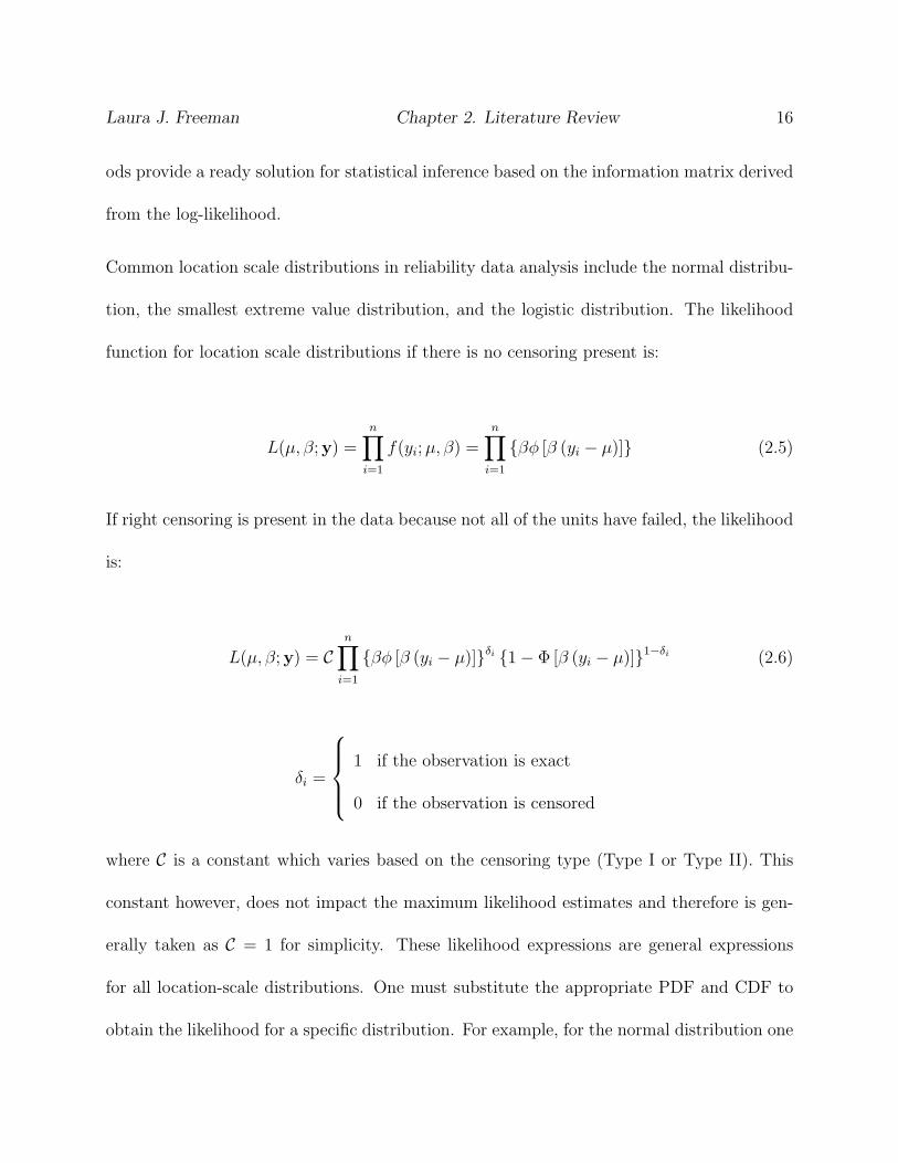
Common location scale distributions in reliability data analysis include the normal distribu-
tion, the smallest extreme value distribution, and the logistic distribution. The likelihood
function for location scale distributions if there is no censoring present is:
L(µ, β; y) =n∏i=1
f(yi;µ, β) =n∏i=1
{βφ [β (yi − µ)]} (2.5)
If right censoring is present in the data because not all of the units have failed, the likelihood
is:
L(µ, β; y) = Cn∏i=1
{βφ [β (yi − µ)]}δi {1− Φ [β (yi − µ)]}1−δi (2.6)
δi =
1 if the observation is exact
0 if the observation is censored
where C is a constant which varies based on the censoring type (Type I or Type II). This
constant however, does not impact the maximum likelihood estimates and therefore is gen-
erally taken as C = 1 for simplicity. These likelihood expressions are general expressions
for all location-scale distributions. One must substitute the appropriate PDF and CDF to
obtain the likelihood for a specific distribution. For example, for the normal distribution one
Laura J. Freeman Chapter 2. Literature Review 17
would use φ = φNorm (the PDF for the normal distribution) and Φ = ΦNorm (the CDF for
the normal distribution). The likelihood can easily be adapted to accommodate left censor-
ing or interval censoring by multiplying the likelihood by additional terms if these types of
censoring are present. The right censored likelihood is presented here because it is the most
common type of censoring in reliability data analysis.
To find the maximum likelihood estimates, the likelihood is then maximized with respect
to the model parameters µ and β. Typically, we maximize the log-likelihood function for
simplicity of calculations. Numerical methods are used to maximize the likelihood expression
with respect to µ and β except in cases where a closed form solution exists. The resulting
estimates for µ and β are the maximum likelihood estimates denoted by µ and β.
Maximum Likelihood Method for Log-Location Scale Distributions
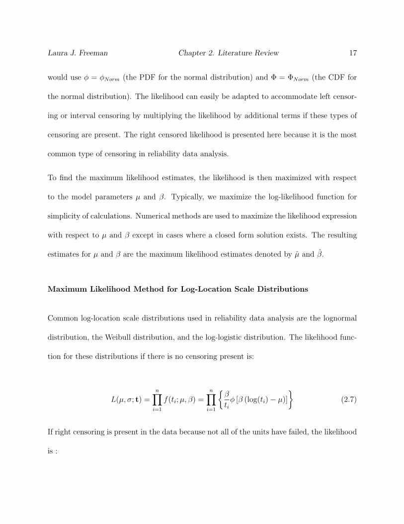
Common log-location scale distributions used in reliability data analysis are the lognormal
distribution, the Weibull distribution, and the log-logistic distribution. The likelihood func-
tion for these distributions if there is no censoring present is:
L(µ, σ; t) =n∏i=1
f(ti;µ, β) =n∏i=1
{β
tiφ [β (log(ti)− µ)]
}(2.7)
If right censoring is present in the data because not all of the units have failed, the likelihood
is :
Laura J. Freeman Chapter 2. Literature Review 18
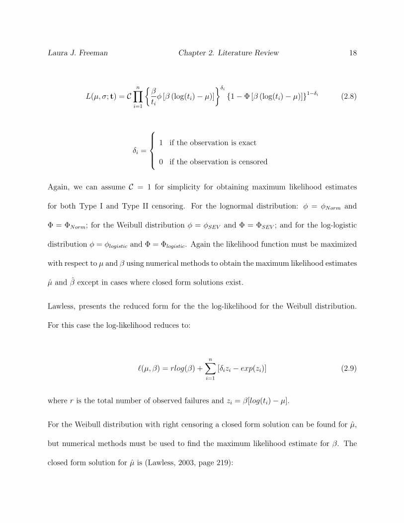
L(µ, σ; t) = Cn∏i=1
{β
tiφ [β (log(ti)− µ)]
}δi{1− Φ [β (log(ti)− µ)]}1−δi (2.8)
δi =
1 if the observation is exact
0 if the observation is censored
Again, we can assume C = 1 for simplicity for obtaining maximum likelihood estimates
for both Type I and Type II censoring. For the lognormal distribution: φ = φNorm and
Φ = ΦNorm; for the Weibull distribution φ = φSEV and Φ = ΦSEV ; and for the log-logistic
distribution φ = φlogistic and Φ = Φlogistic. Again the likelihood function must be maximized
with respect to µ and β using numerical methods to obtain the maximum likelihood estimates
µ and β except in cases where closed form solutions exist.
Lawless, presents the reduced form for the the log-likelihood for the Weibull distribution.
For this case the log-likelihood reduces to:
`(µ, β) = rlog(β) +n∑i=1
[δizi − exp(zi)] (2.9)
where r is the total number of observed failures and zi = β[log(ti)− µ].
For the Weibull distribution with right censoring a closed form solution can be found for µ,
but numerical methods must be used to find the maximum likelihood estimate for β. The
closed form solution for µ is (Lawless, 2003, page 219):

Laura J. Freeman Chapter 2. Literature Review 19
µ =1
βlog
(1
r
n∑i=1
e(β log(ti))
)(2.10)
Other Estimation Methods
Other estimation methods are available for the parameter estimation. Nelson (1990) provides
a descriptions of least squares (LS) estimation methods for complete data. Median rank re-
gression (MRR) is a special case of LS estimation that is detailed in Abernathy (2004). A
significant amount of literature exists on different estimation methods for the Weibull distri-
bution, see for example Hossain and Howlader (1996), who compare least squares estimation
to maximum likelihood estimation. Somboonsavatee, Nair, and Sen (2007) also compare
least squares estimation to maximum likelihood estimation in terms of mean square error.
LS estimation and MRR were very popular in the early lifetime data analysis because of
the simplicity of calculations required. More recently however, these other methods are
losing momentum due to increased availability of computing power. Nelson, Lawless, and
Meeker and Escobar prefer maximum likelihood methods because they can be applied to a
wide range of data types. Additionally, they can easily incorporate censored data into the
analysis, which is extremely important for lifetime data. Maximum likelihood estimates are
also asymptotically optimum and functions of MLEs are also MLE by the invariance property
of MLEs. For all of these reasons the focus of this literature review will be on maximum
likelihood estimation methods despite the availability of additional estimation methods.

Laura J. Freeman Chapter 2. Literature Review 20
Inference for Location Scale and Log-Location Scale Models
Wald’s Method can be used to find confidence intervals on µ and β for the location scale and
log-location scale distributions. It is reasonable to assume that µ is asymptotically normal
because it is already on the log scale, but because β is a positive parameter, it is common
practice to use a log transformation. Therefore, the confidence interval for β is derived using
the delta method. The (1− α)100% confidence intervals for µ and β are respectively:
[µ− z1−α
2ˆs.e.(µ), µ+ z1−α
2ˆs.e.(µ)
](2.11)
[βw, wβ
](2.12)
where, w = z1−α2
ˆs.e.(β)
β. The standard error of the estimates come from the inverse of the
estimation of the parameter’s Fisher’s Information matrix. The information matrix for the
location scale and log-location scale parameters is:
Σ =
V ar(µ) Cov(µ, β)
Cov(β, µ) V ar(β)
(2.13)
=
−∂2`(µ,β)∂µ2 −∂2`(µ,β)
∂µ∂β
−∂2`(µ,β)∂µ∂β
−∂2`(µ,β)∂β2
−1

Laura J. Freeman Chapter 2. Literature Review 21
where the partial derivatives of the log-likelihood are evaluated at the maximum likelihood
estimates µ and β. It is important to note that for the Weibull distribution a significant
correlation between the two parameters exists. The standard error of each of the parameters
is then given by the square-root of its variance estimate in Σ. Alternative methods for com-
puting confidence intervals given by Meeker and Escobar, Lawless and Nelson include using
the likelihood ratio method of computing confidence intervals and Monte-Carlo simulation.
Invariance Property of Maximum Likelihood Estimates
Often in reliability data analysis, the end goal of the analysis is not to predict the distribution
parameters but instead to predict some scalar function, f(µ, β), of the distribution param-
eters. For example, a common function of interest in reliability data analysis is the failure
time for the pth percentile. The pth percentile for the two-parameter Weibull distribution is:
tp = exp
[µ+
Φ−1SEV (p)
β
](2.14)
The invariance property of maximum likelihood estimates ensures us that any function of
the MLEs is the maximum likelihood estimate for that function. Therefore, the MLE of the
pth percentile is:
tp = exp
[µ+
Φ−1SEV (p)
β
](2.15)

Laura J. Freeman Chapter 2. Literature Review 22
The standard error for tp can then be calculated using the multivariate delta method. The
multivariate delta method states that if f = f(θ) then the standard error of f is:
Σf =
[∂f(θ)
∂θ
]TΣ ˆθ
[∂f(θ)
∂θ
](2.16)
The invariance property of maximum likelihood estimates is another reason that they are
very popular and useful for estimating parameters. From the multivariate delta method we
can derive the standard error for tp to be:
s.e.tp = tp
[V ar(µ)− 2
Φ−1SEV (p)
β2Cov(µ, β) +
[Φ−1SEV (p)
β2
]2
V ar(β)
]1/2
(2.17)
2.1.2 Location Scale and Log-Location Scale Regression Models
The maximum likelihood methods of Section 2.1.1 deal with fitting a particular distribution
to failure times. In the previous section, we estimated the distribution’s parameters based
on failure time data. In this section, we are interested in if these distributional parameters
depend on some explanatory variables. Some notation will assist in the following discussion.
• The vector of the failure time distribution parameters will be represented by θ, for
location scale and log-location scale distributions θ =
µ
β
.
• The failure times are denoted by the vector t for log-location scale models and by the

Laura J. Freeman Chapter 2. Literature Review 23
vector y for location scale models
• The explanatory variable(s) will be represented by the matrix Xnxp, where p is the
number of regression model parameters.
• The regression model parameters will be represented by the vector γpx1 = (γ0, γ1, ..., γp−1)T .
In reliability data analysis often the explanatory variable of interest is an accelerating fac-
tor. This section deals solely with statistical issues of the failure time regression analysis.
Accelerated life tests are discussed in the next section.
Coefficient Estimation for the Simple Linear Regression Model
Meeker and Escobar and Lawless focus on modeling the location parameter, µ, as a function
of the regression factors as an appropriate method for translating the effect of the factors in
a designed experiment to the failure times. The simplest possible model for translating the
factors of a designed experiment to failure times is the simple linear regression model. This
section discusses this model for the location scale and log-location scale distributions.
The likelihood function for a sample of n observations with right censoring is:
L(γ0, γ1, β; y) = Cn∏i=1
{βφ [β(yi − µi)]}δi {1− Φ [β(yi − µi)]}1−δi (2.18)
where µi = γ0+γ1xi and δi = 1 for an exact failure and δi = 0 for a right censored observation.
Choosing Φ determines the shape of the distribution. Note that C is a constant which varies

Laura J. Freeman Chapter 2. Literature Review 24
based on the censoring type that is generally taken as C = 1 for simplicity because it does
not impact the maximum likelihood estimation. Also, notice that this likelihood can be
generalized to uncensored data if all δi = 1. We maximize the likelihood function with
respect to γ0, γ1 and β to obtain the MLEs.
The log-location scale regression model for simple linear regression is very similar to the
model for the location scale regression. The likelihood function for a sample of n observations
with right censoring is:
L(γ0, γ1, β; t) = Cn∏i=1
{β
tiφ [β(log(ti)− µi)]
}δi{1− Φ [β(log(ti)− µi)]}1−δi (2.19)
where µi = γ0 + γ1xi and δi = 1 for an exact failure and δi = 0 for a right censored
observation. The likelihood function is maximized with respect to γ0, γ1 and β to obtain
the MLEs. Numerical methods must now be used to maximize the likelihood function. For
the Weibull distribution a partial closed form solution no longer exists now that the location
parameter is a function of experimental factors.
Inference for Simple Linear Regression Model
Wald’s method can again be used to calculate confidence intervals on the model parame-
ters. These confidence intervals require the estimation of the parameter’s Fisher Information
matrix. For the simple linear regression case when θ = (γ0, γ1, β)T the Information matrix
is:

Laura J. Freeman Chapter 2. Literature Review 25
Σθ =
V ar(γ0) Cov(γ0, γ1) Cov(γ0, β)
Cov(γ0, γ1) V ar(γ1) Cov(γ1, β)
Cov(γ0, β) Cov(γ1, β) V ar(β)
(2.20)
=
(−∂2`(γ0,γ1,β)
∂γ20
−∂2`(γ0,γ1,β)∂γ0∂γ1
−∂2`(γ0,γ1,β)∂γ0∂β
−∂2`(γ0,γ1,β)∂γ0∂γ1
−∂2`(γ0,γ1,β)
∂γ21
−∂2`(γ0,γ1,β)∂γ1∂β
−∂2`(γ0,γ1,β)∂γ0∂β
−∂2`(γ0,γ1,β)∂γ1∂β
−∂2`(γ0,γ1,β)∂β2
where the partial derivatives are evaluated at the MLEs, γ0, γ1 and β. The standard error
of each of the parameters is the square-root of its variance estimate in Σ ˆθ. These standard
errors are then used to construct confidence intervals and statistical tests for γ0, γ1 and β.
Again, the confidence interval for β is on the log scale.
From Σ ˆθthe variance for µ and the covariance between µ and β can be calculated using
statistical properties of variance and covariance:
V ar(µ) = V ar(γ0) + x21V ar(γ1) + 2x1Cov(γ0, γ1) (2.21)
Cov(µ, β) = Cov(γ0, β) + x1Cov(γ1, β) (2.22)
Then the delta method can be implemented to calculate standard errors for functions of µ

Laura J. Freeman Chapter 2. Literature Review 26
and β making inference on additional quantities possible. The standard error for tp can now
be calculated using Equation 2.17 just as it was before.
Coefficient Estimation for Multiple Regression Model with Nonconstant Vari-
ance
The maximum likelihood methods described in the simple linear regression section of this
literature review can be extended to more general models. Meeker and Escobar examine
models with multiple linear regression links to the location parameter as well as models with
nonconstant variance. Matrix notation allows for the discussion of more general models.
Let,
µi = xT[µ]iγ [µ] (2.23)
βi = xT[β]iγ [β] (2.24)
It is important to note for total generality the explanatory variables in the location model can
be different from those in the scale model, also the two models can have different dimensions.
These quantities are then used in place of µi and βi in the same likelihood as the simple
linear regression model likelihood. The resulting function is maximized with respect to each
of the model parameters. However, because of complications with maximizing the likelihood
function with respect to a large number of parameters, it is common to assume a constant
Laura J. Freeman Chapter 2. Literature Review 27
scale parameter (i.e. βi does not depend on any regressors). Additionally, this assumption
makes sense from an engineering perspective as long as the failure mechanism is not expected
to change due to the levels of the explanatory variables.
In addition to estimation becoming more difficult when there are multiple factors that impact
both the location and scale parameters, inference becomes tricky as well. The covariance
matrix Σ ˆθis now a larger matrix calculated in a similar fashion to the covariance matrix
for the simple linear regression model. It is easy to see that a large number of predictive
variables quickly complicates the analysis and can result in information matrices that may
not have inverses. For this reason it is important to have an engineering reason for expanding
beyond simple models. Well designed experiments may also be able to assist in appropriate
model selection.
2.1.3 Accelerated Life Test Models
Often in reliability data analysis designed experiments for failure time data fall into the class
of accelerated life tests (ALT). Accelerated life tests run test subjects at more extreme levels
of the design factors than the test subjects would ever encounter under normal use. These
experimental factors are called accelerating factors in an ALT. The goal of an ALT is to
produce more failures than would be seen running an experiment under normal operating
conditions. These tests are an important set of designed experiments in today’s world as
products become more reliable and therefore less likely to fail.

Laura J. Freeman Chapter 2. Literature Review 28
The key to analyzing ALT data is to determine the linearizing relationship between the
accelerating factor and the parameters of the distribution being used to model the failure
time. Nelson and Meeker and Escobar focus on the most appropriate way to relate the
accelerating factor back to the failure distribution as being through the location parameter,
µi. Three common relationships for relating the accelerating factor to the location parameter
are:
• The Arrhenius Relationship for temperature acceleration xi = 11605Tempi(degKelvin)
• The inverse power relationship for voltage and/or stress acceleration xi = log(StressRatio) =
log(V olt(High)V olt(Low)
)
• The generalized Eyring relationship for one or more non-thermal accelerating variable,
dependent on the number of variables and the accelerating factor (i.e. humidity or
voltage)
It is important for the linearizing relationship to be based in engineering knowledge otherwise
the model fit could be completely nonsensical. The methodology for modeling data from
ALTs is:
1. Linearize the factors through an engineering based relationship
2. Fit model using techniques derive in section 2.1.2
3. Transform back results for interpretability in terms of design space for accelerating
factors

Laura J. Freeman Chapter 2. Literature Review 29
2.2 Analysis Techniques for Exponential Family Dis-
tributions
In this section a brief description of the current literature for exponential family distribution
is presented. The goal of this section is to provide insights from how these already well
developed techniques for exponential families might be applied to the Weibull distribution.
The section covers generalized linear models, linear mixed models, and generalized linear
mixed models. McCulloch and Searle (2001) provide a straight forward approach to each
of these topics. These models are important to this proposal because the generalized linear
mixed model theory will provide the motivating theory for the proposed research.
2.2.1 Generalized Linear Models (GLM)
Nelder and Wedderburn (1972) introduces the area of generalized linear models (GLM).
Many statisticians use GLM techniques for the analysis of non-normal data in response
surface experiments. Lewis, Montgomery and Myers (2001) provide three examples where
the response distribution is non-normal. They show that using a GLM analysis results in
better results than transforming the data. Myers and Montgomery (1997) provide a tutorial
for using GLM methods for designed experiments.
GLM analysis is applicable for any distribution that is a member of the natural exponen-
tial family, which includes the binomial, Poisson, normal, logistic, gamma, and exponential

Laura J. Freeman Chapter 2. Literature Review 30
distributions. However the Weibull distribution, which is a popular distribution for reliabil-
ity data analysis, is not a member of the exponential family. The lognormal distribution,
another distribution commonly used in reliability data analysis, is a member of the general
exponential family through its log relationship to the normal distribution.
GLM analysis requires the specification of three model elements :
• Response distribution
• Link function
• Linear predictors
A common choice for the link function is the canonical link. The canonical link equates the
location parameter of the exponential family, µ, to the linear predictor, Xβ. Table 2.1 below
provides the canonical link function for several common exponential family distributions and
the corresponding model parameters.
Table 2.1: Canonical Links for Commonly Used Exponential Family DistributionsDistribution Canonical Link ModelNormal µ = Xβ µ = XβPoisson log(µ) = Xβ µ = exp(Xβ)
Binomial log(
µi1−µi
)= xTi β µi = 1
1+exp(xTi β)
Exponential 1µi
= xTi β µi = 1
xTi β
Many different procedures have been developed for estimating the model parameters of
a GLM. Myers and Montgomery (1997) provide a discussion of iterative re-weighted least

Laura J. Freeman Chapter 2. Literature Review 31
squares which is equivalent to maximum likelihood procedures. Parameter testing and model
inference can use one of three available tests, likelihood ratio test, score test, and Wald’s
Method. All three tests asymptotically follow a χ2 distribution.
2.2.2 Linear Mixed Models (LMM)
A linear mixed model contains both random and fixed effects. The fixed effects model the
mean of the data while the random effects control the structure of the variance-covariance
matrix. Mixed modeling allows the analysis of complicated designs such as blocked designs,
split plot designs and repeated measurement designs by selecting the appropriate fixed and
random effects. McCulloch and Searle (2001) provide an in depth discussion on the analysis
of linear mixed models.
Model and Analysis
Let X be the known model matrix for the fixed effects and β be the vector of fixed effects.
Similarly, let Z be the known model matrix for the random effects and u be the vector of
random effects. Then we can write:
E[y|u] = Xβ + Zu (2.25)
for any realized value of the random vector, u. However, because u, is a random variable we
must assign it probabilistic properties. The common assumption is u ∼ N(0,D), therefore

Laura J. Freeman Chapter 2. Literature Review 32
E[u] = 0 and V ar(u) = D. There is no loss of generality by assuming E[u] = 0 because
if the mean is actually different from zero the variable can be treated as both a fixed and
random factor. The probabilistic assumption for u determines the distribution for y. For
example, suppose the response, y, follows a normal distribution in a linear mixed model,
and u follows a normal distribution(u ∼ N(0,D)),then
y ∼ N( Xβ, ZDZT + R ) (2.26)
where R = V ar(y|u). Note that the fixed effects only impact the mean and the random
effects only impact the variance.
Maximum likelihood or restricted maximum likelihood (REML) are the most common meth-
ods used to find the parameter estimates. McCulloch and Searle (2001) provide a discussion
of the differences between the two estimation methods and the merits of each method. REML
takes the degrees of freedom for estimating the fixed effects into account. This especially
important when the rank of X is large compared to the sample size. REML is also invariant
to the levels of the fixed effects. It does not however estimate the fixed effects directly where
maximum likelihood does. ANOVA estimation methods are also possible in select linear
mixed models. ANOVA methods of estimation which were used historically are now seldom
implemented because solutions are only available for limited cases of linear mixed models.

Laura J. Freeman Chapter 2. Literature Review 33
Split Plot Analysis - Example of a Linear Mixed Model
Vining, Kowalski and Montgomery (2005) discuss the need for split-plot structures in re-
sponse surface designs when one or more hard to change factors are of interest. The split-
plot design provides a practical solution for practitioners faced with time consuming setting
changes that are necessary to implement a completely randomized design. Many researchers
have implemented split-plot designs in industrial response surface experiments and mixture
experiments including Bisgaard (2000), Cornell (1988) and Kowalski, Cornell and Vining
(2002). Jones and Nachtsheim (2009) discuss the prevalence and importance of split-plot
designs in the industrial experimentation.
Split-plot designs can be analyzed using a linear mixed model analysis. To use a linear
mixed model to analyze a split-plot design the whole plot is treated as a random factor and
a variance components covariance structure is placed on the random factor. Therefore,
D =
σ2WP1
0 . . . 0
0 σ2WP2
0 . . . 0
... 0. . . 0
0 . . . 0 σ2WPk
(2.27)
where k is the number of whole plots. This change to the variance-covariance structure of
the response along with Satterthwaites approximation for degrees of freedom allows for the
whole plot factor to be tested using the correct experimental error. Kowalski, Parker and

Laura J. Freeman Chapter 2. Literature Review 34
Vining (2007) provide an example as well as a tutorial for using split-plot designs.
2.2.3 Generalized Linear Mixed Models (GLMM) and Nonlinear
Mixed Models (NLMM)
Model Specification GLMM
Generalized linear mixed models are a logical extension from generalized linear models and
linear mixed models. In generalized linear mixed modeling random factors can be incorpo-
rated with non-normal responses. McCulloch and Searle outline the model specification for
a generalized linear mixed model as:
yi|µ ∼ indep.fYi|µ(yi|µ) (2.28)
where fYi|µ(yi|µ) is from the exponential distribution. Additionally, the conditional mean
of yi is given by:
E[yi|µ] = µi (2.29)
and the link function relating the conditional mean to the fixed and random factors is given
by:
g(µi) = xTi β + zTi u (2.30)

Laura J. Freeman Chapter 2. Literature Review 35
The model specification is complete by choosing a distribution for the responses and the
random effects. McCulloch and Searle recommend maximum likelihood estimation for opti-
mizing the likelihood function for a generalized linear mixed model. The likelihood function
for any distribution is given by:
L(β,u) =
∫ ∏i=1
f1Yi|U(yi|u)f2U(u)du (2.31)
Note the assumption here is that for a given value of the random variable the observations are
independent, but they are not necessarily independent between different levels of the random
factor. This allows for more complicated experimental error structures to be modeled.
McCulloch and Searle provide a very brief introduction to nonlinear mixed models. GLMMs
are a subset of NLMM because NLMM allow the random effect to enter the model through
any of the model parameters as opposed to just the mean. NLMM methodologies prove
to be especially useful in this research because the mean of the Weibull distribution is a
combination of two model parameters. Therefore, introducing the random effect through a
model parameter, not the mean, is more intuitive for the Weibull distribution.
Computational Methods for Integration over the Random Effect
Numerical integration techniques have been substantially researched and applied to Gener-
alized Linear Mixed Models (GLMMs) and Nonlinear Mixed Models (NLMMs). McCulloch
and Searle provide many useful tips and ideas for computational methods for maximizing

Laura J. Freeman Chapter 2. Literature Review 36
the likelihood function with respect to the model parameters which is not a trivial task. A
breif summary of the three primary techniques considered for this dissertation are covered
in this literature review.
Brief Overview of Methods
There are three prominent methods for maximizing the likelihood of a NLMM: (1)Markov
Chain Monte Carlo (MCMC) methods, (2)Quasi-likelihood inference; and (3)Numerical
Quadrature. We discuss all three groups of techniques briefly here. Ultimately, Gauss-
Hermite quadrature was chosen as the numerical integration method used in this research
and the motivations for choosing this method are presented here.
Markov Chain Monte Carlo
MCMC methods can be used to stochastically converge on the MLE for NLMMs. McCulloch
and Searle (2001) discuss several approaches for sampling from a difficult to calculate density.
If MCMC methods are used to find the MLE of the Weibull distribution mixed model, one
would want to use the Metropolis-Hastings sampling algorithm because of the unsymmetrical
nature of the Weibull distribution. MCMC methods use random draws and acceptance
criteria to make draws from the conditional NLMM distribution allowing us to stochastically
converge on the MLE for the NLMM. A brief algorithm for implementing the M-H MCMC
is outlined below.

Laura J. Freeman Chapter 2. Literature Review 37
Sample MCMC Algorithm:
1. Choose starting values for the fixed parameters and the variance.
2. Sample from the conditional distribution (Metropolis-Hastings step).
3. Update the parameters if you meet some acceptance criteria (defined by Metropolis).
4. Update step.
The algorithm repeats for a large number of steps (typically N > 10, 000), then we remove
the burn-in runs (up to 5000). The MLEs of the NLMM are found by averaging the values
over the MCMC draws after the draws stabilize. There are many modifications that can be
made to this algorithm to improve convergence including using expectation maximization
(EM) in step 3 to update the parameters or using simulated annealing to prevent convergence
of the algorithm on a local maximum instead of a global maximum.
This method was quickly ruled out for our application because it does not provide an ap-
proximate closed form solution of the log-likelihood. An important aspect of this research is
the ability to make inferences on the parameter estimates of the Weibull distribution. We
implement likelihood based inference methods which require a closed form approximation
of the likelihood. MCMC methods, while simple to implement, avoid the evaluation of the
integral over the random effect completely; therefore, they do not provide a ready method
for performing inference on the MLEs.

Laura J. Freeman Chapter 2. Literature Review 38
Quasi-Likelihood Methods
Quasi-likelihood (QL) methods and their ability to obtain unbiased consistent estimates of
the MLE are discussed in the literature in great detail including: Lin and Breslow (1996),
Pinheiro and Bates (1995), Breslow and Lin (1995), and Breslow and Clayton (1993). QL
methods approximate the likelihood using a Laplace approximation. The most common
method discussed by Barndorff-Nielson and Cox (1989) expands the integrand using a Taylor
series approximation. The Taylor series approximation is centered at the value of the random
effect which maximizes the approximate log-likelihood. After applying the Taylor series
approximation, QL applies a Laplace approximation to the approximate integrand. The
Solomon-Cox approximation expands the integrand about the true mean of the random
effect (zero), in a Maclaurin series as opposed to a Taylor series (Solomon and Cox, 1992).
Penalized-Quasi Likelihood (PQL) is similar to a quasi-likelihood function except a “penalty”
is added to the likelihood approximations. The penalty term that Green (1987) and Breslow
and Clayton (1993) subtract from the log-likelihood is: u2i /(2σu). The penalty term prevents
arbitrarily large values of the random effect from being selected. McCulloch and Searle (2001)
refer to the penalty as a shrinkage effect. Much of the research comparing approximation
methods focuses on PQL as opposed to quasi-likelihood.
PQL was seriously considered for our application of a NLMM where the responses follow a
Weibull distribution. The mathematical details, however, for PQL methods do not work as
well for the Weibull distribution as they do for exponential family distributions because a

Laura J. Freeman Chapter 2. Literature Review 39
closed form solution does not exist for the likelihood maximizing value of the random effect.
Numerical Quadrature
Gauss-Hermite quadrature is used when the random effect follows a normal distribution. If
the random effect is non-normal, quadrature techniques are limited. Gauss-Hermite quadra-
ture in discussed in detail and compared to PQL in the literature, see for example, Rau-
denbush, Yang and Yosef (2000) and Pinheiro and Bates (1995). Gauss-Hermite quadrature
approximates the integral over the random effect in the likelihood as a weighted sum of the
integrand at a specific number of evaluation points. Abramowitz and Stegun (1964) provide
the tables of the quadrature points and corresponding weights. In recent years, however,
these weights are calculated via mathematical software. The quadrature points are deter-
mined by the roots of the Hermite polynomials and the corresponding weights are given by
the following:
wk =2n−1n!
√π
n2[Hn−1(xk)]2
where Hn(x) is a Hermite polynomial of degree n.
Gauss-Hermite quadrature was the other approximation seriously considered for the Weibull
model with a random effect incorporated into the log-scale parameter, again because it
provides a closed form solution of the approximate log-likelihood for inference. The mathe-
matical details for this method are provided in Chapter 4 of the dissertation.

Laura J. Freeman Chapter 2. Literature Review 40
Additional Methods
There are other methods addressed in the literature for approximating the likelihood. They
include: simulated maximum likelihood, which is discussed briefly by McCulloch and Searle
(2001) as well as linearization methods which are implemented by SAS in PROC GLIMMIX.
Additionally, there are more stochastic approximation algorithms available in addition to
MCMC including genetic algorithms.
2.3 Design of Experiments for Lifetime Data
2.3.1 Lifetime Data Designs
The following criteria provide a framework for discussing planning issues for life tests:
• How many units should you test?
• How long should you run the test?
In lifetime data experimental designs, key requirements for assessing the above criteria are
prior values (or planning values) for µ and β to get a ballpark idea of the distribution shape.
These values should be based on the knowledge of the engineer or scientist that works with
the units to be tested. The literature implements two different approaches for calculating
sample sizes for life tests: Monte Carlo simulation and large sample variance approximations
for maximum likelihood estimators.

Laura J. Freeman Chapter 2. Literature Review 41
The following pseudo code outlines a Monte Carlo for calculating sample sizes:
• Use the planning values of the µ and β and the corresponding distribution to simulate
data for a given sample size
• Analyze the data and construct standard errors and confidence intervals to assess
precision
• Repeat with several different distribution choices and planning values for µ and β
• Repeat the whole process with different sample sizes to gauge actual sample size and
test length requirements
From this Monte Carlo simulation, one will be able to select a test length and sample size
to achieve the desired precision.
The large sample variance approximation is another method for calculating sample size for
life tests. The large sample variance approximations are convenient for determining sample
size because they allow for a closed form relationship relating sample size to the precision of
the estimates. The large sample variance approximation method can also be easily adapted
through use of the delta method so that the sample size calculation be done to minimize the
standard error for some function of µ and β, for example the estimation of the pth percentile,
which is often of practical interest. The information matrix for the large sample variance
approximation is presented in Section 2.1.1 and given by Equation 2.13.

Laura J. Freeman Chapter 2. Literature Review 42
2.3.2 Accelerated Life Test Plans
Planning accelerated life tests require many more decisions and assumptions than planning
life tests do. A key idea behind planning accelerated life tests is that often they need to be
completed within tight time and cost constraints. Another key idea behind accelerated life
tests is that they should always minimize the amount of extrapolation necessary from the
life test levels of the accelerating variables to the use levels of the accelerating variables.
Again, in planning accelerated life tests certain information is necessary to make educated
choices about the life test design. This planning information includes the expected distribu-
tion that the failures follow, planning values for µ and β, and the accelerating relationship
between failure times and the accelerating variable.
Planning Accelerated Life Tests for One Accelerating Variable
To specify an accelerated life test with one accelerating variable one must specify:
• The feasible range of the accelerating variable: [xU , xH ], where xU is the usage level of
the accelerating variable and xH is the highest level where the accelerating relationship
holds for the accelerating variable.
• The total number of units available for the accelerated life test: n
• The number of levels of the accelerating variable
• The allocation of the total number of units to each of the levels of the accelerating

Laura J. Freeman Chapter 2. Literature Review 43
variable.
Again, Monte Carlo simulation or large sample variance approximations are useful in plan-
ning the accelerated life test. These two methods determine the allocation of the units to
different levels of the accelerating variable.
Meeker and Escobar provide a brief discussion of statistically optimum plans which choose
the levels of the accelerating variable and corresponding unit allocation to minimize variance
of the maximum likelihood estimates. Statistically optimum plans can be based on several
different planning criteria. Two common criteria are minimizing the standard error for a
particular percentile or minimizing the determinant of the Fisher information matrix, Iθ.
However, these plans often fail to meet practical constraints of accelerated life tests.
Meeker and Escobar (1998) make some general recommendations for accelerated life test
plans that are not necessarily statistically optimum but preserve some of the design recom-
mendations of statistically optimum plans. Their recommendations include:
• Use insurance units. Insurance units are not expected to fail because they are run at
the expected use levels of the accelerating variable. Insurance units are used to check
for other possible failure modes.
• Use three or four levels of the accelerating variable (this way if one level has problems
there are still two or three levels left for the regression analysis)
– Possible problems are:

Laura J. Freeman Chapter 2. Literature Review 44
∗ A particular level ends up having no failures in the test
∗ A level fails to follow the accelerating relationship
• Choose the lowest level of the accelerating variable subject to the constraint of seeing
four or five failures to help protect against the possibility of having no failures.
• Allocate a higher percentage of units to lower levels of the accelerating variable to
account for the fact that fewer will failures will occur at lower levels of the accelerating
variable
Planning Accelerated Life Tests for Two Accelerating Variables
Meeker and Escobar provide a discussion of planning accelerating life tests for two acceler-
ating variables. For planning an accelerated life test in two explanatory variables, planning
values of the parameters guide the planning process.
Three types of test plans are present in the literature for two explanatory variables:
1. Test all units at normal use level conditions
• This is only a feasible test plan if the goal is to predict a relatively low failure
percentile and the probability of failure for a particular unit is high
2. Test at two or more combinations of the variable levels along a line that passes through
the use conditions and the maximum conditions for each of the accelerating factor
• This test plan does not allow for the full specification of the regression model

Laura J. Freeman Chapter 2. Literature Review 45
3. Test at three or more non-collinear combinations of the experimental variables.
The third test plan allows for the full specification of the regression model, which makes
it the best test plan to implement; however, the first two test plans can provide valuable
information, especially in a pilot study.
Planning Accelerated Life Tests in More than Two Variables
Accelerated life tests for more than two accelerating variables require complicated accelerat-
ing relationship and well as design plans. Meeker and Escobar advocated using traditional
design of experiments designs for these types of accelerated life tests including the factorial
design.
2.3.3 Response Surface Designs
Response surface designs are very popular in an industrial setting because they seek to
optimize the response using small sample sizes. A first order design is the first step in
the sequential RSM process. The common first order designs are the full factorial, 2k, and
the fractional factorial, 2k−p, designs. These designs are presented in great detail in Myers
and Montgomery (2002). Myers and Montgomery also provide many other RSM designs
including Box-Behnken, Plackett-Burman, and central composite designs (CCDs).
Hamada (1995) discusses using several common response surface designs in reliability ex-
periments. These designs include full factorial designs, fractional factorial designs and the

Laura J. Freeman Chapter 2. Literature Review 46
Box-Behnken design. He uses the maximum likelihood methodologies outlined in Section
2.1 to analyze the data obtained in these experiments. However, in several of the designs
replication is present. Hamada fails to discuss whether the replicates are true replicates or
if they are observational units. He treats all of the experimental errors as independent and
identically distributed despite the fact that in a few of the experiments it is highly unlikely
that pure replication occurred. This is great area for improvement in the current reliability
data analysis methodologies as very little attention has been focused on correctly modeling
experimental error versus modeling observational error.
McCool (1996) and McCool and Baran (1999) have also looked at estimating the parameters
for a Weibull distribution for designed experiments. They focus on 22 factorial experiments,
which are common response surface designs. McCool and Baran provided an analysis that
begins to take the experimental design into account in their paper by fitting four different
Weibull distributions using maximum likelihood estimation to each level of the 22 factorial
experiment. This approach however does not fully incorporate the data into one model or
provide a methodology for testing the significance of the factorial experiment parameters.
2.4 Literature Review Summary
This literature review covered many seemingly disjoint topics ranging from current methods
of lifetime data analysis, to generalized linear mixed modeling. The goal of this research is
to combine the well developed statistical techniques of GLMMs and NLMMs with reliability

Laura J. Freeman Chapter 2. Literature Review 47
data analysis. An area of concern in this research is the proper modeling of experimental error
and observational error for the complicated designs that are commonly used in reliability
data analysis. Another key issue is censoring. Censored data is nearly impossible to avoid
when dealing with reliability data and needs to be accounted for in both the experimental
design and the experimental analysis. Another important consideration for this research is
the correlation between the parameters of the Weibull parameters noted by many reliability
researchers. The next two chapters provide two new analysis methods based in the foundation
of this literature review.

Chapter 3
Two-Stage Analysis Solution
3.1 Introduction and Current Modeling Approach
This chapter presents a two-stage analysis method that utilizes current statistical theory to
analyze reliability data. This new proposed method is nice because it provides a statistically
straightforward approach to handling complicated design structures. The analysis methods
presented in this chapter utilize the maximum likelihood approach for analyzing reliability
data applied to the Weibull distribution. The current modeling approach is first presented as
a means of comparison for a new modeling approach that is presented second. The general
form of the likelihood function is:
L(β, µ) =N∏i=1
[f(ti)] (3.1)
48

Laura J. Freeman Chapter 3. Two-Stage Analysis 49
where f(ti) is the probability density function (PDF) for the Weibull distribution. A key
assumption in the derivation of this likelihood function is that the N observations are inde-
pendent. We compute the log-likelihood to find:
`(β, µ) =N∑i=1
log [f(ti)] (3.2)
In reliability analysis a common goal is to determine the impact of experimental factors
on product lifetime, most approaches focus on the best method for modeling the impact
of the experimental factors is through the scale parameter. Therefore, the log of the PDF
for the Weibull distribution, incorporating the dependance of the scale parameter on the
experimental factors, can be expressed as:
log [f(ti)] = log
(β
ti
)+ zi − exp(zi) (3.3)
where zi = β [log(ti)− µi], µi = log(ηi) = xTi γ, and xTi is the 1 x p vector of experimental
factors for a given experimental run. Plugging the PDF for the Weibull Distribution into
the log-likelihood we find the final form for the log-likelihood:
`(β, γ) =N∑i=1
[log
(β
ti
)+ zi − exp(zi)
](3.4)
This log-likelihood function can then be maximized with respect to β and γ to obtain the

Laura J. Freeman Chapter 3. Two-Stage Analysis 50
maximum likelihood estimates.
If the data contain right censoring, the log-likelihood for the Weibull distribution reduces to:
`(β, γ) =N∑i=1
δi
[log
(β
ti
)+ zi
]− exp(zi) (3.5)
This likelihood is then maximized with respect to β and γ. This method is implemented in
many statistical packages including Minitab, which is used in this paper in an illustrative
example. Note that an important assumption that for both the uncensored and right censored
likelihood derivations is that the observations are independent, therefore the treatments must
be randomly applied to each test unit for this assumption to hold true.
3.2 New Modeling Approach
Our modeling approach is based on two fundamental concepts in design of experiments
(DOE), experimental units and observational units. The experimental unit is the smallest
unit to which the treatment is applied. The observational unit is the unit where the mea-
surement is taken. A common design protocol in reliability experiments is to place n items
on a a test stand and apply a given treatment combination to the test stand. For example,
consider a temperature-humidity chamber which is used to test the shelf life of food prod-
ucts. The chamber holds n units. Suppose a food science engineer is interested in the impact
of different temperature and humidity settings on the shelf life of chips. He places n bags

Laura J. Freeman Chapter 3. Two-Stage Analysis 51
of chips in m different chambers and selects a temperature and humidity setting for each
chamber. In this experiment the chamber is the experimental unit, and the bags of chips are
the observational units. The total sample size is N = nm.
Experimental units and observational units are important concepts from DOE because they
provide the basis for calculating experimental error correctly. The experimental units provide
the basis for estimating the experimental error, which is the appropriate basis for all inference
involving the experimental factors. The observational error contributes to the experimental
error but only in part and, therefore, does not provide an appropriate basis for inferential
procedures. The impact of confusing the observational units with the experimental units
is manifold. First, if we treat the observational units as experimental units in the design
described above we will be calculating the experimental error incorrectly which directly
impacts standard error of the parameter estimates and all inferences made in the statistical
analysis. Second, we will be overstating our true degrees of freedom. Therefore, when we
make inferences about the significance of the experimental factors, we use an error term
that is too small and overstate the significance of the factor. Additionally, this error is
transmitted to the shape parameter estimate of the lifetime distribution because we are
failing to model the experimental error correctly. If the experiment is looking purely at
accelerating factors then the parameter estimates at the accelerated conditions will impact
the predicted performance at use conditions.
The model we propose is a two-stage model that is a simple first approach to account for
the experimental error correctly. This model assumes that there are n items placed on m

Laura J. Freeman Chapter 3. Two-Stage Analysis 52
different test stands. Each treatment combination is applied to the test stand, and the
measurements are made on each of the n items. The assumptions underlying the model are:
• The lifetimes for the individual units within a test stand follow a Weibull distribution.
• The failure mechanism for each treatment combination is the same (i.e. β is constant
across test stands).
• The impact of the treatments is realized through the scale parameter.
• The test stands are independent.
• The experimental variability between the scale parameters for each treatment combi-
nation is lognormal.
3.2.1 Stage 1 Model: The model within an experimental unit:
Let tij be the observed lifetime for the jth item within the ith test stand. The failure times
follow a Weibull distribution within a test stand, therefore:
f (tij) =β
ηi
(tijηi
)β−1
e−(tijηi
)β(3.6)
for a given test stand. Here β > 0 is the constant shape parameter and ηi is the scale
parameter for test stand i. It can be shown that if tij follows a Weibull distribution, then
the likelihood for given test stand where all of the n items fail is:

Laura J. Freeman Chapter 3. Two-Stage Analysis 53
L(β, µi) =n∏j=1
f(tij) (3.7)
We can find the MLEs for β and the ηi’s by maximizing the joint log-likelihood over all m
test stands. The log-likelihood over the m test stands for uncensored data is:
`(β, µ1, . . . , µm) =m∑i=1
n∑j=1
(log
(β
tij
)+ zij − ezij
)(3.8)
where zij = β [log(tij)− µi] and µi = log(ηi).
Right censoring can also be easily incorporated into the likelihood function. The likelihood
for an individual test stand with right censoring present is:
L(β, µi) = Cn∏j=1
[f(tij)]δij [1− F (tij)]
1−δij (3.9)
where δij = 1 if the item fails and δij = 0 if the item is censored. Again, C is a constant
dependent on the type of censoring but can be take as C = 1 when calculating maximum
likelihood estimates. The joint log-likelihood for data with right censoring then becomes:
`(β, µ1, . . . , µm) =m∑i=1
n∑j=1
(δij log
(β
tij
)+ δijzij − ezij
)(3.10)
The first stage in the analysis results in the MLE for the common shape parameter, β and

Laura J. Freeman Chapter 3. Two-Stage Analysis 54
m MLEs for the scale parameter for each test stand. Additionally, under certain regular-
ity conditions, an asymptotic variance-covariance matrix can be derived for the maximum
likelihood estimates. Meeker and Escobar (1998) note that the Weibull distribution meets
these regularity conditions. The estimated covariance matrix for the maximum likelihood
estimates is:
Σθ =
V ar(β) Cov(β, µ1) . . . Cov(β, µm)
Cov(β, µ1) V ar(µ1)...
.... . . Cov(µm−1, µm)
Cov(β, µm) . . . Cov(µm, µm−1) V ar(µm)
(3.11)
=
−∂2`(β,µ1,...,µm)∂β2 −∂2`(β,µ1,...,µm)
∂β∂µ1. . . −∂2`(β,µ1,...,µm)
∂β∂µm
−∂2`(β,µ1,...,µm)∂β∂µ1
−∂2`(β,µ1,...,µm)
∂µ21
...
.... . . −∂2`(β,µ1,...,µm)
∂µm−1∂µm
−∂2`(β,µ1,...,µm)∂β∂µm
. . . −∂2`(β,µ1,...,µm)∂µm∂µm−1
−∂2`(β,µ1,...,µm)∂µ2
m
−1
From the log-likelihood it can be shown that:
−∂2`(β, µ1, . . . , µm)
∂β2=
m∑i=1
n∑j=1
[δijβ2
+
(zijβ
)2
exp(zij)
](3.12)

Laura J. Freeman Chapter 3. Two-Stage Analysis 55
−∂2`(β, µ1, . . . , µm)
∂β∂µi= −
n∑j=1
(2zijβ
exp(zij)
)(3.13)
−∂2`(β, µ1, . . . , µm)
∂µ2i
=n∑j=1
(β2 exp(zij)
)(3.14)
Additionally, the 2nd derivatives between all pairs of µi and µj are zero. This variance matrix
will be used in the second stage of the model. These equations for the estimated variance
matrix hold true for both uncensored and censored data if you note that δij = 1 for all points
in the uncensored data case.
3.2.2 Stage 2 Model: The model between experimental units:
After obtaining the estimates for the shape parameter and the scale parameters and their
corresponding variances for each experimental unit, the next step is to model the estimates
of the scale parameters as a linear function of the treatments. An appropriate second stage
model that accounts for the variances on the scale parameter estimates is a weight least
squares model. The second stage model is:
µ = Xθ + ε (3.15)
where X is the matrix containing the treatment levels of the factors, θ are the corre-

Laura J. Freeman Chapter 3. Two-Stage Analysis 56
sponding coefficients that relate the treatment levels to the log of the scale parameter and
ε ∼ MVN(0,V), where the variance matrix, V, accounts for the scale parameter vari-
ance estimates. Since this variance matrix is near diagonal a reasonable assumption is to
use V =< V ar (µi) > and then parameter estimates are given by the normal solution for
weighted regression model:
θ =(XTV−1X
)−1XTV−1µ (3.16)
The big advantage to this approach is that you can correctly model the experimental error
in current statistical packages that have the ability to fit lifetime distribution and linear
models.
3.3 Percentile Predictions
A quality of interest to industrial statisticians is the prediction of the failure percentiles.
Calculating the percentiles provides us with a practical implication to base the comparison
between the old method and our newly proposed method. The MLE for the pth percentile
is:
tpi = exp
[µi +
Φ−1SEV (p)
β
](3.17)

Laura J. Freeman Chapter 3. Two-Stage Analysis 57
where ΦSEV (p) is the inverse CDF for the smallest extreme value distribution and µi =
log(ηi) = xTi γ. In addition, to calculating the predicted percentiles it is often useful to have
bounds on these percentiles for practical implications. The normal approximation confidence
interval based on Wald’s Method for tp is:
100(1− α)%CI =
[tp/w, wtp
](3.18)
where, w = exp(z1−α
2
ˆs.e.(tp)
tp
). The standard error of tp can be estimated using the multi-
variate delta method and is:
ˆs.e.(tp) = tp
[V ar(µ)− 2Φ−1
SEV (p)
β2Cov(µ, β) +
[Φ−1SEV (p)
β2
]2
V ar(β)
]1/2
(3.19)
The variance and covariance for µ and β come from straightforward functions from the
estimated variance matrix based on the inverse Fisher’s Information matrix for γ and β. For
example, if µi = log(ηi) = γ0 + γ1x1i + γ2x2i, then:
V ar(µ) = V ar(γ0)+x21V ar(γ1)+x
22V ar(γ2)+2x1Cov(γ0, γ1)+2x2Cov(γ0, γ2)+2x1x2Cov(γ1, γ2)
Cov(µ, β) = Cov(γ0, β) + x1Cov(γ1, β) + x2Cov(γ2, β)
For the new two-stage analysis proposed in this paper it is easy to modify this expression

Laura J. Freeman Chapter 3. Two-Stage Analysis 58
for tp to calculate the estimated percentiles:
tpi = exp
[xTi θ +
Φ−1SEV (p)
β
](3.20)
The confidence interval is again given by Equation 3.18 and the standard error is given by
Equation 3.19. However, the calculation of the values for the Fisher Information matrix here
is not possible because the estimates come from two completely disjoint likelihood functions.
This is a major disadvantage of the two stage approach because only inferences on the
parameters of the distribution are possible.
3.4 Illustrative Example
Zelen (1959) discusses a factorial experiment designed to determine the effect of voltage and
temperature on the lifespan of a glass capacitor. Zelen describes the experimental setup
as “n components are simultaneously placed on test.” This experimental setup provides a
perfect data set to compare the traditional reliability analysis to the proposed analysis, which
accounts for the experimental protocol. Table 3.1 summarizes the data from the experiment.
Zelen uses two different temperature settings and four different voltages in the experiment for
a total of 8 treatment combinations. Each treatment combination is applied to only one test
stand, making this an unreplicated experiment from a DOE perspective. Eight capacitors
are tested on each test stand, and Zelen uses Type II censoring after the first four failures.

Laura J. Freeman Chapter 3. Two-Stage Analysis 59
Table 3.1: Life Test Results of Capacitors, Adapted from Zelen (1959)
3.4.1 Results: Traditional Analysis
Meeker and Escboar (1998, page 447-450) provide the traditional reliability analysis for
the Zelen data, which are summarized in Table 3.2 using Minitab’s Lifetime data analysis
function. Note that in this analysis, the estimate of the shape parameter is β = 2.75. The
analysis indicates that voltage and temperature both have a significant impact on the scale
parameter and therefore the lifetime of the glass capacitor.
Table 3.2: Independent Analysis for Life-test on Glass Capacitors, Adapted from Meekerand Escobar (1998)
Regression Table
Standard 95.0% Normal CI
Predictor Coef Error Z P Lower Upper
Intercept 13.4070 2.29584 5.84 0.000 8.90726 17.9068
Voltage -0.0059108 0.0010398 -5.68 0.000 -0.0079488 -0.0038729
Temperature -0.0289047 0.0128970 -2.24 0.025 -0.0541822 -0.0036271
Shape 2.74869 0.418739 2.03917 3.70509
Log-Likelihood = -244.242
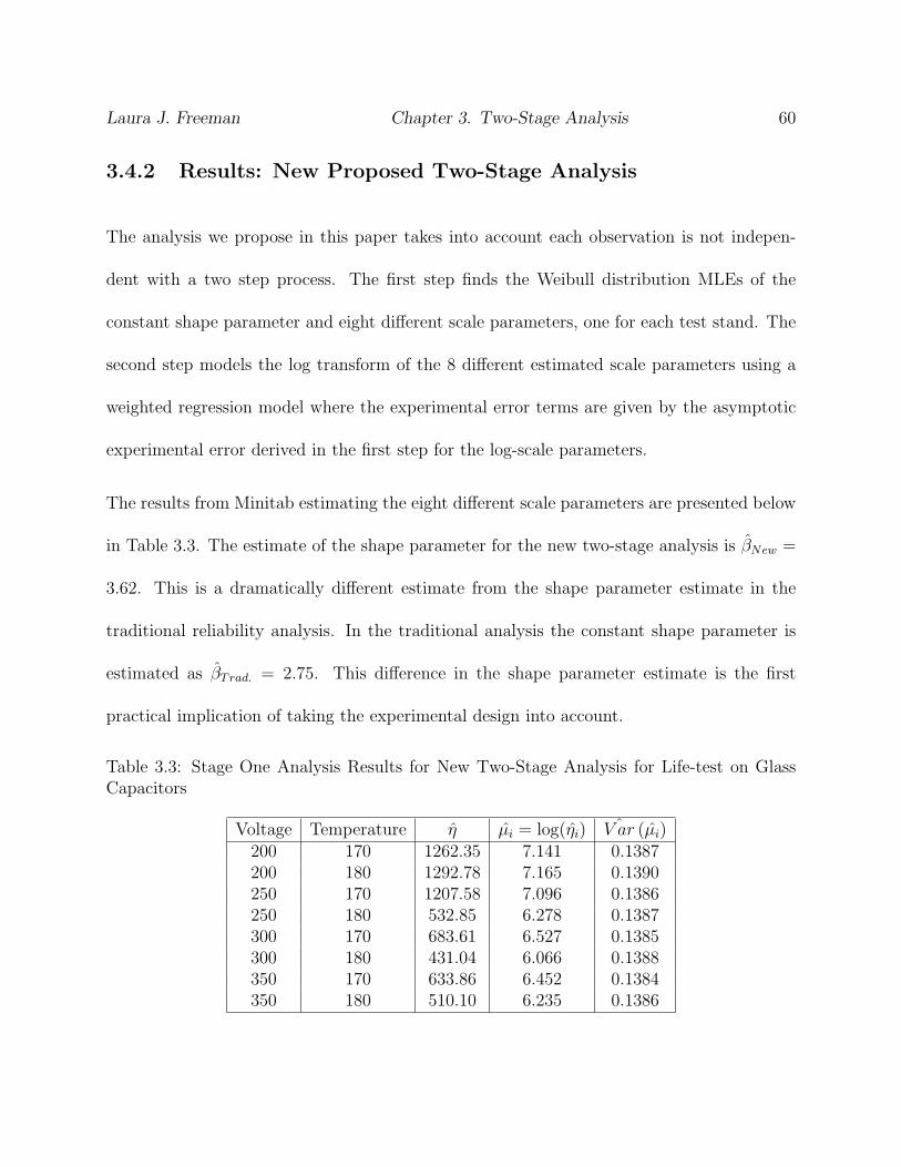
Laura J. Freeman Chapter 3. Two-Stage Analysis 60
3.4.2 Results: New Proposed Two-Stage Analysis
The analysis we propose in this paper takes into account each observation is not indepen-
dent with a two step process. The first step finds the Weibull distribution MLEs of the
constant shape parameter and eight different scale parameters, one for each test stand. The
second step models the log transform of the 8 different estimated scale parameters using a
weighted regression model where the experimental error terms are given by the asymptotic
experimental error derived in the first step for the log-scale parameters.
The results from Minitab estimating the eight different scale parameters are presented below
in Table 3.3. The estimate of the shape parameter for the new two-stage analysis is βNew =
3.62. This is a dramatically different estimate from the shape parameter estimate in the
traditional reliability analysis. In the traditional analysis the constant shape parameter is
estimated as βTrad. = 2.75. This difference in the shape parameter estimate is the first
practical implication of taking the experimental design into account.
Table 3.3: Stage One Analysis Results for New Two-Stage Analysis for Life-test on GlassCapacitors
Voltage Temperature η µi = log(ηi) ˆV ar (µi)200 170 1262.35 7.141 0.1387200 180 1292.78 7.165 0.1390250 170 1207.58 7.096 0.1386250 180 532.85 6.278 0.1387300 170 683.61 6.527 0.1385300 180 431.04 6.066 0.1388350 170 633.86 6.452 0.1384350 180 510.10 6.235 0.1386

Laura J. Freeman Chapter 3. Two-Stage Analysis 61
The second step of our proposed new analysis models the resulting MLEs for the µi’s using
a weighted regression model where the weights are determined by the asymptotic variances
from the first step of this model. The second stage of this analysis can be done in any standard
statistical package. Note that the variance estimates on the different µi are essentially equal
in Table 3.3. This is a nice result because in the second stage of the model, using a weighted
regression is essentially equivalent to standard least squares regression, further simplifying
this two stage analysis method. This is the case because we have assumed a constant shape
parameter, β, and the shape parameter is the driving parameter in the Fisher Information
matrix calculations for the variances on the scale parameters, see Equation 3.12. The results
from running the analysis in Minitab are displayed in Table 3.4.
Table 3.4: Stage Two Analysis Results for New Two-Stage Analysis for Life-test on GlassCapacitors
Regression Table
Predictor Coef SE Coef T P
Constant 14.613 3.249 4.50 0.006
Voltage -0.005638 0.001644 -3.43 0.019
Temperature -0.03682 0.01838 -2.00 0.102
S = 0.0359013 R-Sq = 75.9% R-Sq(adj) = 66.3%
Several practical differences emerge comparing the results of the new analysis back to the
traditional analysis. The standard errors of the coefficients are all smaller in the traditional
analysis. This is because we were overstating the true experimental degrees of freedom
by treating each observation as an independent data point. The increase in standard error

Laura J. Freeman Chapter 3. Two-Stage Analysis 62
Table 3.5: Independent Analysis Percentile Predictions and Confidence Intervals for Life-teston Glass Capacitors
results in the temperature not being a significant factor at α = 0.05 level for the new analysis.
Additionally, the estimates of the shape parameter are dramatically different between the two
analysis methods. The coefficient estimates for the linear relationship between the log-scale
parameter and temperature and pressure are also slightly different.
3.4.3 Impact on Percentile Estimation
The following tables compare the 1st, 5th, 10th and 50th percentiles. To provide a fair means
of comparison, for both percentile estimates we use temperature and voltage as predictors of
the scale parameter, even though temperature is not significant at the α = 0.05 level for the
new analysis. In Table 3.5 the percentile estimates and their corresponding Wald confidence
intervals are displayed for the traditional maximum likelihood analysis.

Laura J. Freeman Chapter 3. Two-Stage Analysis 63
Table 3.6: New Two-Stage Analysis Percentile Predictions for Zelen Data
In Table 3.6 the percentile predictions for the new analysis are given. The percentiles for the
new analysis predict fewer failures early on, that is the first through the tenth percentiles have
later predicted times. The fiftieth percentile however, occurs earlier for the new analysis.
These changes in the percentile predictions make clear the impact of the change in the
shape parameter estimate. Confidence intervals are not available because the inverse of the
information matrix does not exist. In comparing the percentile estimates for the new method
back to the confidence bounds, one can see that the percentile estimates are significantly
different between the two methods. These differences are driven by the different shape
parameter estimates for the two methods.
3.5 Conclusions from Two Stage Model Solution
This proposed methodology is just a first, naive approach to trying to combine the experi-
mental protocol with reliability data analysis. The goal of this chapter was to illustrate that
the experimental design has a nontrivial impact on the conclusions drawn when modeling

Laura J. Freeman Chapter 3. Two-Stage Analysis 64
lifetime data with a Weibull distribution. The first implication is that we fail to correctly
calculate the experimental error term if we base the experimental error on the observational
units instead of the experimental units. This miscalculation will result in a lower experi-
mental error because variation between observational units is inherently lower than between
experimental units. Furthermore, if we incorrectly treat observational units as experimen-
tal units, we overstate the degrees of freedom for experimental error. The other important
impact of fitting the correct model to the experimental setup is that this translates into
the shape parameter estimate. In the example presented in this chapter, the shape param-
eter dramatically shifted between the two analysis methods, which for a practitioner could
lead to dramatically different conclusions about the failure mechanism to which a product
succumbs.
There is a good deal of room for improvement with this analysis method. This new approach
is designed for a practitioner to be able to use now. In fact, the proposed analysis can already
be done in the current version of Minitab and other common statistical packages. The only
complicating factor is that the asymptotic variances need to be calculated by hand and then
entered into Minitab. In the example presented in this chapter however, the variances are
essentially equal and therefore do not impact the estimation and the full analysis can be done
directly in current software packages. A clear next step in this research is to fully combine
the estimation into a joint likelihood. This two step model is easy to implement but is most
like not the optimum way to model the data. A joint likelihood approach for β and ηi’s
would mostly likely result in more precise estimates of the parameters. Additionally, a joint

Laura J. Freeman Chapter 3. Two-Stage Analysis 65
likelihood approach would provide the ability to perform likelihood based inferences on not
just the parameters but also functions of the parameters.

Chapter 4
Nonlinear Mixed Model Analysis
4.1 Introduction
Random effects arise from many DOE choices; these choices include sub-sampling, clustered
data, random selection of the treatment levels, and blocking. It is important to have an
analysis methodology that can properly handle these different experimental designs for life
data. This chapter presents a new maximum likelihood analysis method to incorporate
random effects into the analysis of life test data from a sub-sampling experimental design.
We implement our new analysis method on the Zelen data and run a simulation study to
further investigate the implications of properly including random effects in the data analysis.
Feiveson and Kulkarni (2000) note the need to incorporate a random effect into the model
when batch effects are present in the data. Their data, originally from Gerstle and Kunz
66

Laura J. Freeman Chapter 4. NLMM Analysis 67
(1983), measures burst times for Kevlar fiber strands at accelerated stress levels. The fiber
strands encase pressure vessels on the Space Shuttle, and therefore, their reliability is of
paramount importance. The strands are manufactured in spools, which result in a batch
effect based on the spool. Feiveson and Kulkarni emphasize the need for modeling the batch
effect as a random effect because there are only eight spools tested in the experiment; yet,
the space shuttle pressure vessels could have fiber strands from any number of manufactured
spools. They incorporate random effects through a stratified least squares approach.
Leon, Ramachandran, Ashby, and Thyagarajan (2007) also note the need for random effects
in accelerated life tests of fiber strands that come from different batches. They also use data
from Gerstle and Kunz (1983) to justify their model. They propose a Bayesian modeling
approach for incorporating the random spool effect and conclude that the random model
results in “better” estimates and predictions than the corresponding model that treats the
spool as a fixed effect. They also note that both the fixed and random effect models result in
a practically different estimate of the Weibull shape parameter than if the analysis ignores
the batch completely. The lesson they highlight is that ignoring a vital parameter, such as
spool in their case, results in bias of the shape parameter.
Leon, Li, Guess and Sawhney (2009) conduct a simulation study based on the same fiber
strand data. They use the Bayesian modeling methods developed by Leon et. al (2007).
They conclude that ignoring the batch effect results in overly precise estimates of quantiles
and probabilities of failures.
In Chapter 3 of the dissertation, we propose a naive method to take into account the ex-

Laura J. Freeman Chapter 4. NLMM Analysis 68
perimental protocol for a sub-sampling DOE through a two-stage analysis method. While
this method is simple and straightforward to implement, it is flawed in that there is no joint
likelihood, and therefore, inferences on functions of the parameters are not possible. Addi-
tionally, this two-stage method is susceptible to bias in the estimate of the shape parameter
and it is limited to the sub-sampling experimental design. The method proposed in this
chapter addresses the joint likelihood problem from Chapter 3 by incorporating a random
effect into the model.
4.2 Nonlinear Mixed Model Methodology
4.2.1 Model
We propose a frequentist model for incorporating the random effects into the failure time
model. Our specification assumes that the random effect is due to sub-sampling, but this
approach is easily adaptable to the Gerstle and Kunz (1983) data, where the random effect
is due to a batch effect.
One commonly incorporates random effects into a model in one of two ways; through the
mean response or through the model parameters. Generalized linear mixed models (GLMMs)
use the first method. Nonlinear mixed models (NLMM) are more flexible and transmit the
random effect through model parameters. For the Weibull distribution, a common assump-
tion is that all model terms (treatments, blocks, etc.) enter through a linear relationship with

Laura J. Freeman Chapter 4. NLMM Analysis 69
the log-scale parameter. Therefore, we are using the NLMM framework for incorporating a
random effect. McCulloch and Searle (2001, 286-290) provide a general outline of NLMM.
If we have i = 1, . . . ,m independent experimental units and j = 1, . . . , ni sub-samples or
observational units per experimental unit, we can specify our nonlinear mixed model for the
Weibull distribution with sub-sampling as:
tij|ui ∼ Indep. Weib(β, ηi)
F1(tij|β, ηi, ui) = 1− exp
[−(tijηi
)β]log(ηi) = µi = xTi θ + ui
f2(ui) ∼ iid N (0, σ2u)
where xi is the p x 1 vector of fixed factor levels, θ is the vector of fixed effect coefficients,
and ui are i = 1, ...,m independent random effects.
The likelihood for uncensored data for the given model specification is:
L(β,θ|Data) =m∏i=1
∫ ni∏j=1
f1(tij|ui)f2(ui)dui (4.1)
where f1(tij|ui) is the Weibull PDF for the data within an experimental unit and f2(ui) is
the normal PDF for the random effect. This likelihood could be easily adapted to model

Laura J. Freeman Chapter 4. NLMM Analysis 70
different experimental designs. However because sub-sampling is commonly used in design
of experiments for reliability data, this chapter focuses on the sub-sampling random effect
model. If right censoring is present in the data, then the likelihood is:
L(β,θ|Data) =m∏i=1
∫ ni∏j=1
[f1(tij|ui)]δij [1− F1(tij|ui)]1−δij f2(ui)dui (4.2)
In this chapter we focus solely on the likelihood for right censoring because of the preva-
lence of right censoring in reliability data. Additionally, the right censored likelihood easily
reduces to the uncensored likelihood by letting all δij = 1. Random effects models, espe-
cially nonlinear models, pose many computational issues in that in order to maximize the
likelihood because it is necessary to integrate out the random effect ui.
4.2.2 Gaussian Quadrature
There are several different mathematical techniques for integrating out the random effect
for the NLMM. Gauss-Hermite (G-H) quadrature, as discussed in Chapter 2, was selected
as the best method for this research. G-H quadrature is applicable when the random effect
follows a normal distribution. G-H quadrature requires the random effect to have the form
e−x2. Therefore, a change of variables is necessary to apply G-H quadrature to our likelihood
function. Let ui =√
2σuvi, then the likelihood before the change of variables is:

Laura J. Freeman Chapter 4. NLMM Analysis 71
L(β,θ|Data) =m∏i=1
∫ ∞−∞
ni∏j=1
g(tij|ui)e−u2
i2σ2u√
2πσ2u
dui (4.3)
where g(tij|ui) = [f1(tij|ui)]δij [1− F1(tij|ui)]1−δij for right censored data. Executing the
change in variables results in the following likelihood:
L(β,θ|Data) =m∏i=1
∫ ∞−∞
[ni∏j=1
g(tij|√
2σuvi)e−v
2i
√π
]dvi (4.4)
Now we can directly apply G-H quadrature to approximate the likelihood. The G-H quadra-
ture results in the following approximation of the likelihood:
L(β,θ|Data) ≈m∏i=1
1√π
{nk∑k=1
[ni∏j=1
g(tij|√
2σuqki)wk
]}(4.5)
where nk is the number of quadrature points, qk are the evaluation points found from the
roots of the Hermite polynomials, and wk are the corresponding weights to the evaluation
points given by:
wk =2n−1n!
√π
n2[Hn−1(qk)]2.
A common recommendation for the number of quadrature points to minimize bias is 20
points. Pinheiro and Bates (1995) show that G-H quadrature with 100 points is as good
as any other solution they investigated to the numerical optimization problem. In this
research, we use 20 quadrature points in all of our analyses unless otherwise stated. This

Laura J. Freeman Chapter 4. NLMM Analysis 72
limits computation time, especially in the simulation studies. The log-likelihood is:
`(β,θ|Data) ≈m∑i=1
log
(1√π
nk∑k=1
[ni∏j=1
g(tij|√
2σuqki)wk
])(4.6)
The approximate log-likelihood is maximized through standard maximization techniques.
We use quasi-Newton optimization with a Broyden, Fletcher, Goldfard, and Shanno (BFGS)
update of the inverse Hessian matrix.
4.2.3 Inference
An advantage of using G-H quadrature is it results in a closed-form approximate log-
likelihood. Therefore, we can derive a Hessian matrix and asymptotic covariance matrix
from the approximate log-likelihood. Maximum likelihood theory states that under certain
regularity conditions that√n(θ − θ) converges in distribution to a multivariate normal.
Therefore, for our model let θ∗T = [β,θ, σu]. Then, θ∗∼ asymptotically MVN [θ∗, I(θ∗)−1],
where
I(θ∗) =
−∂2`(β,θ1,...,θp,σu)
∂β2 −∂2`(β,θ1,...,θp,σu)
∂β∂θ1. . . −∂
2`(β,θ1,...,θp,σu)∂β∂θp
−∂2`(β,θ1,...,θp,σu)
∂β∂σu
−∂2`(β,θ1,...,θp,σu)
∂β∂θ1−∂
2`(β,θ1,...,θp,σu)
∂θ21
... −∂2`(β,θ1,...,θp,σu)
∂θ1∂σu
.... . . −∂
2`(β,θ1,...,θp,σu)∂θp−1∂θp
...
−∂2`(β,θ1,...,θp,σu)
∂β∂θp. . . −∂
2`(β,θ1,...,θp,σu)∂θp∂θp−1
−∂2`(β,θ1,...,θp,σu)
∂θ2p−∂
2`(β,θ1,...,θp,σu)∂θp∂σu
−∂2`(β,θ1,...,θp,σu)
∂β∂σu−∂
2`(β,θ1,...,θp,σu)∂θ1∂σu
. . . −∂2`(β,θ1,...,θp,σu)
∂θp∂σu−∂
2`(β,θ1,...,θp,σu)∂σ2
u
The estimated covariance for the parameter estimates can be found by substituting the

Laura J. Freeman Chapter 4. NLMM Analysis 73
MLEs into the information matrix, I(θ∗). Meeker and Escobar (1998, page 622) note that
the regularity conditions hold for the Weibull distribution. See Appendix A for the derivation
of the information matrix for the random effects Weibull model.
4.2.4 Software
R-CRAN software is implemented for approximating the likelihood of the Weibull NLMM
and the numerical optimization. Additionally, SAS PROC NLMIXED allows the user to
program in their own likelihood function and specify the number of quadrature points. The
default in SAS NLMIXED is to use adaptive quadrature, which is described in Pinheiro and
Bates (1995). We however, choose to use 20 point G-H quadrature so our R-cran software
results are directly comparable to the SAS NLMIXED results. Both the SAS and the R-cran
code us the BFGS update to the Hessian matrix. However, SAS PROC NLMIXED defaults
to using analytical derivatives for updating the Hessian, while R-cran’s optim function uses
numerical derivatives. These two methods can result in different solutions. We recommend
using the analytic derivatives if possible. Appendix B provides the R-cran code and the SAS
code for analyzing the NLMM.
4.3 Motivating Example
Zelen (1959) provides an example of a classic reliability DOE. Zelen describes a life test
on glass capacitors under two temperature and four voltage settings that a glass capacitor

Laura J. Freeman Chapter 4. NLMM Analysis 74
would experience under normal use. The observational units in this experiment are the
eight glass capacitors on each test stand. The experimental units are the eight test stands,
where the researcher applied the unique temperature, voltage treatment combination. Type
II censoring, after the first four failures, is used for each test stand. Table 3.1 provides the
Zelen data.
Meeker and Ecobar (1998, pages 447-450) provide a life test analysis of the Zelen data
assuming the treatments were independently applied to all 64 capacitors. The results of the
analysis are reproduced in Table 3.2 using Minitab. These results can also be found using
SAS’s Proc LIFEREG. The analysis indicates that voltage and temperature both have a
significant impact on the scale parameter and therefore the lifetime of the glass capacitor.
A basic principle of experimental design is that an experimental design induces a particular
probability structure. If an experiment is not a completely randomized then treating each
observation as independent and multiplying the values of the PDF together to obtain the
likelihood is a violation of the statistical assumptions underlying the model. Additionally,
treating each observation as independent induces the wrong experimental error for testing.
Including a random effect allows us to model the true experimental error and observational
error correctly. In the Zelen data, the eight glass capacitors on each test stand are dependent.
The analysis from Meeker and Escobar (1998) ignores the correlations between the glass
capacitors on the same test stands.
The model specification presented in Section 3 of this paper allows for the sub-sampling
described in the Zelen glass capacitor experimental design. The results from this analysis

Laura J. Freeman Chapter 4. NLMM Analysis 75
using 20 point G-H quadrature to approximate the likelihood are given in Table 4.1.
Table 4.1: Nonlinear Mixed Effects Model Analysis for Life-test on Glass Capacitors
Incorporating random effects into the model results in similar estimates of the shape param-
eter, β, and the model relating temperature and voltage to the log-scale parameter, µi as
the independent analysis. One important difference to note is that all of the standard errors
are larger for the nonlinear mixed effects model. This is because we are properly modeling
our experimental error and observational error in the random effects model. These larger
standard errors result in temperature no longer being a significant term in the model.
Note that we estimate log(σu) as opposed to σu, which helps convergence of the NLMM,
especially in cases where σu is close to zero. The invariance property of MLEs and the delta
method allow us to estimate σu and the standard error of σu. The standard error is:
se (σu) = σuse [log (σu)] (4.7)
The estimate of σu = 0.0489 for the Zelen data is small, but it is still important to include
in the model to ensure that the experimental error is properly modeled.

Laura J. Freeman Chapter 4. NLMM Analysis 76
In Chapter 3 we analyze the Zelen dataset using a two-stage modeling approach, which
properly accounts for the sub-sampling experimental design. The standard errors between
their analysis and the nonlinear mixed model analysis are similar in magnitude. However,
the estimate of the shape parameter in the two-stage analysis is much higher, β = 3.62, than
either the independent analysis or the NLMM analysis indicating that the two-stage method
is susceptible to bias in the estimation of the shape parameter.
4.4 Monte Carlo Simulation Study
While the Zelen data provides an interesting application of the random effects model, it fails
to fully investigate the impact of using the random effect model over the independent model.
A particular “shortfall” in the data is that the estimated variance on the random effects
is small. However, since there is no true replication in Zelen data, the variance may only
appear to be small due to the experimental protocol.
Recall, in the random effects model, we incorporate the treatment combinations and the
random sub-sampling error into the model through the log-scale parameter, log(ηi) = µi =
xTi θ + ui. In the Zelen data, the researcher applies each unique temperature, voltage treat-
ment combination to only one test stand. Therefore, the fixed effects and the random
sub-sampling variance are confounded and cannot be uniquely estimated. A reasonable con-
jecture, especially because these data were collected in 1959, is that variability between test
stands is actually higher than we found in the above analysis. The simulation study pre-

Laura J. Freeman Chapter 4. NLMM Analysis 77
sented here investigates the impact of different levels of variance on the random effect as well
as the impact of model misspecification on the NLMM. We compare the NLMM results to
the independent model analysis results.
4.4.1 Simulation Design
We base the simulation study heavily on the Zelen data to maintain a realistic experimental
setup. The goal of the simulation study is to determine the impact of the random effect
variance and model specification on the analysis. We investigate model misspecification
because it is a well known fact that the Weibull distribution parameters are correlated. We
wish to investigate how the possible misspecification of the scale parameter impacts that
shape parameter estimate. Leon et. al (2007) observed this impact when the spool effect
was not incorporated into the analysis.
The setting of all parameters for the simulation study are based on the analysis of the original
Zelen data. We coded the temperature and voltage to be in the range [−1, 1] so that the
coefficients can be directly compared. Coding the fixed factor settings does not influence the
estimate of the shape parameter for either the independent analysis or the nonlinear mixed
model analysis.
The simulation study uses the following parameter values: θ0 = 6.7, θvolt = −0.44, θtemp =
−0.44, θvolt∗temp = 0.15 and β = 2.78. We selected these parameter values based on the
NLMM results for the coded Zelen data. We hold these quantities constant across all of

Laura J. Freeman Chapter 4. NLMM Analysis 78
the simulations. The changing settings for the simulation study to investigate the impact of
random effect variance and model misspecification are:
• σ2u = [0.01, 0.1, 1], the variance of the random effect.
• wm = [0, .5, 1], the weight of the model misspecification. Note when wm = 0 there is
no model misspecification and when wm = 1 the model misspecification is the most
severe
• Assumed Model
– Model 1: contains voltage and temperature (θvolt = −0.44, θtemp = −0.44)
– Model 2: contains voltage, temperature and positive interaction (θvolt = −0.44,
θtemp = −0.44, θvolt∗temp = 0.15)
The lowest value is approximately twice as large as the estimated value for the Zelen data
NLMM from Table 4.1. We base the largest variance on the maximum Weibull variance
for the parameter estimates from Chapter 3. The final value, σu = .316 =√.1, provides a
mid-value for the variance.
The simulation study uses a full factorial design, resulting in 18 (3× 3× 2) simulation runs.
We maintain the same experimental design as the original Zelen data, eight test stands each
with eight capacitors, Type II censoring for each test stand after the fourth failure. We run
10,000 replications of the simulation study to ensure a small simulation error.

Laura J. Freeman Chapter 4. NLMM Analysis 79
We executed the Monte Carlo simulation study in SAS. We generated the random effects
within a test stand using the rand(“normal”) statement built into SAS. We generated the
Weibull data within a test stand using the inverse CDF method and the rand(“uniform”)
built into SAS. We stored the both the nonlinear mixed model solution for each run and
the independent model solution for comparison. We confirmed the SAS results from Proc
NLMIXED as well as Proc LIFEREG through code written by the author in R-cran.
4.4.2 Results
Figure 4.1 shows the results for the estimation of the Weibull shape parameter for the first
simulation model, containing voltage and temperature. In Figure 4.1 the black lines are
results for NLMM analysis and the grey lines are for independent analysis. We applied the
model misspecification weights to temperature in the data generation step and fit the model
containing voltage. Therefore, when wm = 1 the coefficient for temperature used in the data
generation is -0.44, when wm = 0.5, the coefficient is -0.22, and when wm = 0 the coefficient
is 0. The model fit for these cases always contains only voltage. Therefore, when wm = 0,
there is no model misspecification. We present the results for β/β.
Figure 4.2 shows the results for the estimation of the Weibull shape parameter for the second
simulation model, containing voltage, temperature, and their interaction. In this model, we
apply the model misspecification weights to the interaction term. The fit model always
contains the main effects for temperature and voltage. The results for the second model are

Laura J. Freeman Chapter 4. NLMM Analysis 80
Figure 4.1: Monte Carlo Simulation Study Investigating the Impact of Random Effect Vari-ance and Model Misspecification on the Pivotal Weibull Shape Parameter for Model 1
very similar to the first model. Figure 4.2 again presents the results for β/β.
The results for the two different assumed models indicate that the random model results
are nearly invariant to the degree of model misspecification and the variance of the random
effect. The independent model estimates of β get worse as the variance of σu increases and
as the degree of model misspecification increases. The random effects model provides a more
robust estimate of the shape parameter for both model forms considered in this simulation
study.
Often, in reliability data analysis we use pivotal quantities like β/β to generalize results
for all values of beta. We ran the simulation study without any changes to the parameters
except for using the value β = 1 to check if these pivotal quantities hold for this more
complex model. Figure 4.3 shows the results of this study in terms of β/β = β. While

Laura J. Freeman Chapter 4. NLMM Analysis 81
Figure 4.2: Monte Carlo Simulation Study Investigating the Impact of Random Effect Vari-ance and Model Misspecification on the Pivotal Weibull Shape Parameter for Model 2
the general conclusions are the same for this value of β, the actual values are not equal;
therefore, pivotal quantities should be interpreted with caution in this study.
In contrast to the estimates of the shape parameter, the estimates of the coefficients for the
log-scale parameter are relatively robust to the analysis method. Figure 4.4 shows that our
ability to estimate the log-scale parameter linear coefficient is primarily based on the level of
random effect variance and the degree of model misspecification, not the modeling method.
However, the statistical significance of those estimates are heavily dependent on the model
analysis method. Figure 4.5 shows that as σu increases the ability to detect a significant
effect in the model for the log-scale parameter decreases in the independent model more
substantially than it does for the random model. These p-values correspond directly with
the coefficient estimates in Figure 4.4. This decrease in significance is more notable for the
independent case because the independent model is not using the correct experimental error

Laura J. Freeman Chapter 4. NLMM Analysis 82
Figure 4.3: Monte Carlo Simulation Study Investigating the Impact of Random Effect Vari-ance and Model Misspecification for Model 1, β = 1
for inference.
Finally, we note that in the initial Zelen data analysis we suggest that the NLMM under-
estimates the true value of σu. We are unable to confirm this conjecture for the Zelen data
because of the lack of true replication in the data. Therefore, the estimate of σu is completely
confounded with the estimates of θ. In the simulation study we show, how well we estimate
θvolt in Figure 4.4 and the confounded random variance in Figure 4.6. In Figure 4.6 the black
solid line indicates no bias in the estimate of σu.
The results in Figure 4.4 and Figure 4.6 illustrate the importance of replication in the
experimental design. We see that both θvolt and σu are subject to bias however, under the
current experimental design we cannot separate the estimates. If true replicates were present,
we could obtain an estimate of σu independent of the log-scale parameter coefficients.
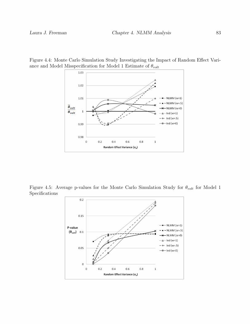
Laura J. Freeman Chapter 4. NLMM Analysis 83
Figure 4.4: Monte Carlo Simulation Study Investigating the Impact of Random Effect Vari-ance and Model Misspecification for Model 1 Estimate of θvolt
Figure 4.5: Average p-values for the Monte Carlo Simulation Study for θvolt for Model 1Specifications

Laura J. Freeman Chapter 4. NLMM Analysis 84
Figure 4.6: Estimated Random Standard Deviation versus the True Value for Monte CarloSimulation Study
4.5 NLMM Conclusions and Future Directions
In this chapter we provide and methodology for incorporating random effects into life test
data where sub-sampling is present. Our simulation study reveals that these models are more
robust to model misspecification and increasing levels of variance in the random effect when
compared to their independent model counterparts. The methods can easily be adapted to
incorporate random effects other than one induced by sub-sampling.
There is a great deal of room for further exploration with these random effect models. In
this paper, we applied the model to a life test experiment with sub-sampling. Clear next
steps involve extending the analysis here to accelerated life tests and additional types of
experimental designs that incorporate random effects.
Additionally, this new modeling technique provides a new framework for thinking about

Laura J. Freeman Chapter 4. NLMM Analysis 85
experimental design for life tests. We note in the Zelen data no true statistical replicates
exist, therefore we cannot uniquely estimate σu and θ in our model. Experimental designs
that allow the full model to be uniquely estimated should be investigated.
Chapter 5
Application of the Principles of
Experimental Design to Reliability
Data
5.1 Introduction
Fisher (1935) in “The Design of Experiments” outlines the three principles for statistical
design of experiments that have guided experimental design and testing for the past 75
years. These principles are: (1) Randomization; (2) Replication; and (3) Local Control of
Error.
The analysis limitations of reliability data have historically forced the analysis of reliability
86

Laura J. Freeman Chapter 5. Experimental Design 87
experiments to assume a completely randomized designs (CRD). However, rarely is this
the case in practice. Jones and Nachtsheim (2009) note how prevalent split-plot deigns
are in industrial experimentation. Reliability experiments have historically focused on the
questions: (1) How many test units should be run? and (2) How long should they be placed
on test? These two questions have dominated the reliability field because of problems with
censored data. Experimental designs outside of CRDs have generally been disregarded in the
reliability community because, until recently, analysis methods were not available to handle
data with more complicated randomization scheme than a CRD.
In previous chapters of this dissertation, we saw an industrial experiment from Zelen (1959)
that was not a completely randomized design because it contained sub-sampling. However,
the Zelen data have been analyzed as a CRD in the reliability literature, which violates the
principles of experimental design. The methodologies developed in Chapters 3 and 4 of this
dissertation provide two different methodologies for properly modeling the randomization
and replication of a sub-sampled experimental design, resulting in different estimates of the
experimental error. Chapter 3’s method is limited to the sub-sampling experimental design
without further modifications. Chapter 4, while structured around the sub-sampling DOE,
could be extended to incorporate other types of error control including blocking and split-plot
designs.
The randomization scheme is of paramount importance in the data analysis, if a design is
not completely randomized it cannot be analyzed as a CRD. We provide two new analysis
techniques that allow the user to properly model data from designs containing sub-sampling.

Laura J. Freeman Chapter 5. Experimental Design 88
Another problem with the Zelen DOE is no true replication exists in the experiment. The lack
of replication in this experiment becomes apparent in the new analysis methods presented for
sub-sampled data. The final principle of experimental design, local control of error, including
blocking, are beyond the scope of this dissertation. However, it is important to correctly
model the experimental error and the observational error, which is the focus of error control
in this dissertation.
This chapter illustrates the implication of randomization, replication and experimental error
in a correctly analyzed reliability experiment. We use the most straightforward experimen-
tal design available for two experimental factors; a 22 factorial design. The Monte Carlo
simulation studies in this chapter provide a limited introduction to the importance of incor-
porating the principles of DOE outlined by Fisher into lifetime tests. Additionally, we look
at testing for the Weibull NLMM derived in Chapter 4 using the correct experimental error.
The estimation of standard errors are central to hypothesis testing. Properly modeling the
experimental error ensures a defendable test. We look at normal approximation hypothe-
sis testing and likelihood ratio tests. Finally, a comparison is made between the different
analysis methods for the Zelen data in terms of estimation, testing and prediction.

Laura J. Freeman Chapter 5. Experimental Design 89
5.2 Monte Carlo Experimental Design Study
5.2.1 Comparison Study between Zelen DOE and 22 Factorial DOE
We use the Zelen (1959) glass capacitor data as the guiding experimental data for explor-
ing the implications of incorporating the principles of experimental design into reliability
experiments. In this chapter, we apply the NLMM analysis methodology from Chapter 4 to
analyze the data from the simulation study.
Recall the model for the sub-sampling DOE in Chapter 4 is:
tij|ui ∼ Indep. Weib(β, ηi)
F1(tij|β, ηi, ui) = 1− exp
[−(tijηi
)β]log(ηi) = µi = xTi θ + ui
f2(ui) ∼ iid N (0, σ2u)
In the Zelen data we note that since there is no true replication, the estimate of the ran-
dom effect standard deviation, σu, is completely confounded with the fixed effect coefficient
estimates. In the first part of the simulation study, we compare the Zelen DOE with a 22
factorial experiment replicated twice. These two experimental designs have the same num-
ber of experimental units and sub-samples. We generate data using the following parameter
values:

Laura J. Freeman Chapter 5. Experimental Design 90
• β = 2.78
• θ0 = 6.7
• θ1 = −0.44
• θ2 = −.44
• σ2u = 0.01, 0.1 and 1.0
These values are the same values used in Chapter 4’s simulation study. The only difference
between the two simulation cases in this Chapter is the experimental designs.
Table 5.1 provides the average MLEs of σu for the NLMM over 10,000 simulation runs. Both
experimental designs dramatically underestimate σu for the case when σu = 0.1. The other
two values of σu are also underestimated but not as severely. There does not appear to be
a difference in the two experimental designs in their ability to estimate the variance of the
random effect, despite the fact that σu is mathematically confounded with θ in the Zelen
DOE and it is not for the 22 factorial DOE.
Table 5.1: Estimates of Random Effect Variance for Monte Carlo Simulation Study Com-paring Zelen Design to Replicated 22 Design
σu σu Replicated Design σu Zelen Design0.1 0.00067 0.00071
0.316 0.1795 0.17901 0.8903 0.8901
Figures 5.1 - 5.3 show the difference in the two experimental designs in the estimation
of the other three model parameters. An important fact to remember about the Weibull

Laura J. Freeman Chapter 5. Experimental Design 91
distribution is that the shape and scale parameters are correlated. Therefore, all of our
parameter estimates are correlated in the NLMM.
Figure 5.1: Pivotal Coefficient Estimate for Weibull Shape Parameter, β, for Zelen Designversus Replicated 22 Factorial Design. Black solid line indicates no bias.
Figure 5.2: Pivotal Coefficient Estimate for Voltage in log-scale Parameter Model for ZelenDesign versus Replicated 22 Factorial Design
The main conclusion from the experimental design comparison study is that neither exper-
imental design outperforms the other in terms of estimation. A strong conjecture of the

Laura J. Freeman Chapter 5. Experimental Design 92
Figure 5.3: Pivotal Coefficient Estimate for Temperature in log-scale Parameter Model forZelen Design Versus Replicated 22 Factorial Design
reason behind this result is that both designs are lacking sufficient degrees of freedom to
estimate σu accurately. In the analysis of the Zelen DOE and the 22 replicated factorial, we
have only seven degrees of freedom for estimation. We need to estimate the fixed parameter
coefficients, the Weibull shape parameter, and the variance of the random effect. Estimating
these terms requires at least three degrees of freedom (2 for the fixed effect, 1 for the random
effect variance). The shape parameter estimate comes from a combination of information
within each sub-sample and between experimental units so a full degree of freedom is not
required to estimate it. However, this only leaves approximately 3 degrees of freedom for
experimental error, if we do not fit an interaction term in the model. The next part of
the simulation study looks at exactly how much replication is needed to obtain unbiased,
consistent estimates of the model parameters.

Laura J. Freeman Chapter 5. Experimental Design 93
5.2.2 Monte Carlo Simulation Study 22 Factorial DOE with Repli-
cation
To analyze the impact of replication on the parameter estimates, we use the same experi-
mental setup as Zelen except we use the 22 Factorial design and replicate it from r = 1 (no
replication) to r = 10. The Zelen data use Type II right censoring; however in reliability
experiments, Type I censoring provides a practical time and cost constraint. Therefore, we
look at both Type I and Type II censoring in the replication study to evaluate their impact
on the parameter estimates.
The Zelen data use Type II censoring after 50% of the glass capacitors fail. Therefore, we
use 50% Type II censoring in the simulation study. In order to compare Type I and Type
II censoring, we base our Type I censoring scheme closely on the Type II censoring scheme.
We calculate the 50% percentile time for each group, resulting in 4 potential censoring times
given in Table 5.2. The average time across all eight groups t.50 = 859 which is used as the
censoring time for the Type I censoring scheme.
Table 5.2: 50% Percentile Estimates for Type I Censoring
Voltage Temperature t.50
-1 -1 1716.71 -1 712.1-1 1 712.11 1 295.3
To further improve our ability to compare between censoring types we apply them to the

Laura J. Freeman Chapter 5. Experimental Design 94
same uncensored data set. In the simulation study, we generate an uncensored dataset, then
both censoring schemes, Type I and Type II, are applied to the uncensored data.
Table 5.3: Expected Number of Failures for Type I Censoring (Censoring Time = 859 Hours)
Voltage Temperature E(Nf )-1 -1 0.76951 -1 5.5114-1 1 5.51141 1 8.0000
In Type I censoring it is possible to observe no failures in a group. Table 5.3 gives the
expected number of failures for each test stand in the 22 factorial DOE. Clearly, in the low
temperature, low voltage test stand, we anticipate the possibility of observing no failures,
which creates an empty cell. In the cases where no failures are observed, we can write the
portion of the approximate log-likelihood for test stand i as:
`i(β,θ|Data) ≈ log
(1√π
nk∑k=1
[ni∏j=1
g(tij|√
2σuxki)wk
])
= log
(1√π
nk∑k=1
[ni∏j=1
exp[− exp(zijk)]wk
])
The above equation shows that there is still a contribution to the log-likelihood for an empty
cell. Additionally, we can still find the maximum likelihood estimates if we observe an empty
cell. However, as we will later note in the simulation study results, we observe that estimates
for the unreplicated design can be of very poor quality. Replication improves the estimates
of the parameters. The impacts of empty cells are investigated more in the full simulation

Laura J. Freeman Chapter 5. Experimental Design 95
study.
Impact of Replication: Type I Censoring
Figures 5.4 - 5.7 show the results for the Type I censored replicated 22 factorial design.
Figure 5.4 shows that the estimates for β are biased above the true value. Replicating the
design a minimum of 4 times appears to give a good quality estimate of the Weibull shape
parameter. The asymptotic properties of the MLE appear to take effect around 4-6 replicates
of the 22 factorial.
Figure 5.4: Pivotal Coefficient Estimate for Weibull Shape Parameter for Replicated 22
Factorial Design with Type I Censoring
Recall, the Zelen experimental design was a motivating factor for the simulation study on
replicated experimental designs. The estimate of σu is confounded with treatment combina-
tions in the NLMM for the Zelen design. Figure 5.5 shows the impact of replication on our
ability to estimate σu. The simulation results show that if σu is small a very large sample
size is required to estimate σu with any accuracy. Even for r = 10, the estimate of σu is

Laura J. Freeman Chapter 5. Experimental Design 96
only approximately 26% of the true value. We are able to estimate σu with a great deal
more accuracy for the larger values. However, for Type I censored data and σu = 1, we
dramatically overestimate σu in the cases where empty cells occur.
Figure 5.5: Pivotal Coefficient Estimate for σu for Replicated 22 Factorial Design with TypeI Censoring
Figures 5.6 and 5.7 show the average estimates of the coefficients for voltage and temperature,
respectively, of the log-scale parameter linear model. For Type I censoring we notice that
these estimates can be very poor when there are empty cells and a small number of replicates.
In fact, the two figures do not contain the estimates for the coefficients for the case when r = 1
and σu = 1. They were omitted because the estimates were 235% and 245% the true values
of the coefficients for voltage and temperature respectively and masked the other points in
the figures. In addition to the log-scale parameter coefficient estimates being of poor quality
in the unreplicated design, we cannot fit interaction term because the main effects model for
log-scale parameter, β and σu result in a fully saturated model. The unreplicated 22 factorial
design is never recommended based on these simulation results. Increasing replication, for

Laura J. Freeman Chapter 5. Experimental Design 97
all values of σu, results in better estimates of the coefficients, θvolt and θtemp, of the log-scale
parameter model. The estimates are within the simulation error of the simulation study for
r ≥ 6.
Figure 5.6: Pivotal Coefficient Estimate for Voltage in log-scale Parameter Model for Repli-cated 22 Factorial Design with Type I Censoring
Figure 5.7: Pivotal Coefficient Estimate for Temperature in log-scale Parameter Model forReplicated 22 Factorial Design with Type I Censoring
In summary, for Type I censored data, 4 replicates of a 22 factorial DOE with 8 sub-samples
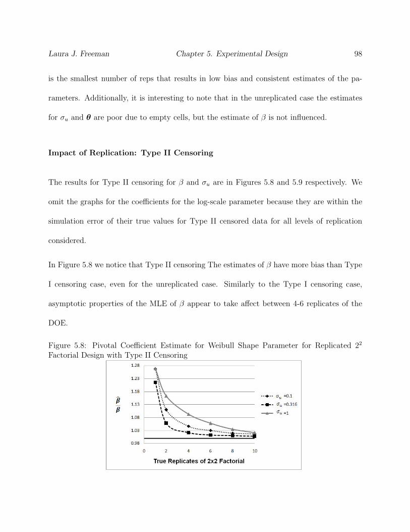
Laura J. Freeman Chapter 5. Experimental Design 98
is the smallest number of reps that results in low bias and consistent estimates of the pa-
rameters. Additionally, it is interesting to note that in the unreplicated case the estimates
for σu and θ are poor due to empty cells, but the estimate of β is not influenced.
Impact of Replication: Type II Censoring
The results for Type II censoring for β and σu are in Figures 5.8 and 5.9 respectively. We
omit the graphs for the coefficients for the log-scale parameter because they are within the
simulation error of their true values for Type II censored data for all levels of replication
considered.
In Figure 5.8 we notice that Type II censoring The estimates of β have more bias than Type
I censoring case, even for the unreplicated case. Similarly to the Type I censoring case,
asymptotic properties of the MLE of β appear to take affect between 4-6 replicates of the
DOE.
Figure 5.8: Pivotal Coefficient Estimate for Weibull Shape Parameter for Replicated 22
Factorial Design with Type II Censoring

Laura J. Freeman Chapter 5. Experimental Design 99
Figure 5.9 contains the simulation study results for the estimate of σu. The results for Type
II censoring are similar to Type I censoring. Our ability to estimate σu is dependent its true
value. For the smallest value of σu, a large sample size is required to estimate the parameter
accurately. A major difference between the two censoring types exists in the unreplicated
case. For Type II censoring we severely underestimate all three values of the σu in the
unreplicated case. For Type I censoring, we severely overestimate σu for the large variance
case and underestimate it for the other two cases.

Laura J. Freeman Chapter 5. Experimental Design 100
Figure 5.9: Pivotal Coefficient Estimate for σu for Replicated 22 Factorial Design with TypeII Censoring
5.2.3 Monte Carlo Simulation Study Conclusions
The results of the design comparison simulation study indicate that neither the Zelen design
nor the 22 factorial design replicated twice is sufficient for estimating the parameters of the
Weibull NLMM, particularly for σu and β. This conclusion led to a replication study of the
22 factorial DOE. The goal was to determine the amount of replication required to provide
accurate estimates of the parameter for the Weibull NLMM. The 22 Factorial DOE was
replicated from 1 to 10 times. The minimum number of replicates that is advisable for this
type of data based on this simulation study is r = 4. The estimates have relatively low bias
at 4 replicates and the asymptotic properties of the MLEs appear to take over.

Laura J. Freeman Chapter 5. Experimental Design 101
5.3 Statistical Testing and Inference
Throughout this dissertation we have used asymptotic covariance matrix and a normal ap-
proximation for testing parameter significance. However, we have also noted through several
different simulation studies, including the replication study in the previous section, that
asymptotic properties are slow to take effect for the Weibull distribution, especially for the
shape parameter. Therefore, the normal approximation for testing parameter significance
may be a poor assumption.
ME and Lawless (2003) recommend normal approximation as well as the likelihood ratio test
(LRT) for testing. In this section, we briefly review the normal approximation theory for
the Weibull NLMM. We derive LRT tests for the NLMM and compare the results between
the two methods.
In this section we propose three different LRTs: (1) for fixed effects; (2) for the random
variance; (3) for lack of fit (LOF). We compared the fixed effects and random effects LRT
back to the large-sample normal approximation test. No LOF test is readily available under
normal approximation. We provide a discussion on the theoretical χ2 distribution of the LRT.
However, this theoretical distribution is a large sample property. Therefore, re-sampling
techniques are proposed as an alternative to the χ2 assumption. Re-sampling techniques
may prove especially useful to practitioners who primarily work with small sample sizes.
Through bootstrapping the data, we can set a cutoff which may prove to be a better test for
parameter significance for small samples.

Laura J. Freeman Chapter 5. Experimental Design 102
5.3.1 Normal Approximation
Recall from Chapter 4 that one can derive a Hessian matrix and asymptotic covariance matrix
from the approximate log-likelihood. Maximum likelihood theory states that under certain
regularity conditions that√n(θ − θ) converges in distribution to a multivariate normal.
Therefore, for our model let θ∗T = [β,θ, σu], then θ∗∼ Asymptotically MVN (θ∗, I(θ∗)−1),
where Equation 4.7 specifies I(θ∗). The estimated covariance for the parameter estimates
can be found by substituting the MLEs into the information matrix, I(θ∗). Meeker and
Escobar (1998, page 622) note that the regularity conditions hold for the Weibull distribution.
Appendix A of the dissertation proves that the first and second derivatives exist and are
continuous for the Weibull NLMM. The derivatives are provided in Appendix A as well.
Inference on the parameters from this information can be done through straightforward z-
tests. The test statistic for testing if a given model parameter is significantly different form
zero is:
z =θ − 0
s.e.(θ)
where s.e.(θ) is the square root of the corresponding diagonal element of the covariance
matrix I(θ∗)−1. Notice that a frame work for a general lack of fit test is not available
under normal approximation. Only tests on the parameters and functions of the estimated
parameters are readily available.

Laura J. Freeman Chapter 5. Experimental Design 103
5.3.2 Likelihood Ratio Test
Likelihood ratio tests are widely applicable tests related to maximum likelihood estimation.
The LRT is defined by a ratio of the likelihood under null hypothesis to the likelihood under
the alternative hypothesis. The test works by setting a cut-off value for the ratio between the
two likelihoods, and if the ratio is less than that cutoff the test rejects the null hypothesis.
Define the deviance of the LRT as D = −2 log(Lnull
Lalt). The deviance is asymptotically χ2
with p degrees of freedom, where p is the number of parameters being tested. Therefore
asymptotically,
D = −2 log(Lnull)− (−2 log(Lalt)) ∼ χ2p (5.1)
We use Monte Carlo simulation to examine the small sample behavior of the deviance for
the three different Weibull NLMM tests. The simulation studies including in the following
sections determine when the χ2p cutoff is reasonable for the 22 factorial designs.
Fixed Effects
The LRT can be used to test the significance of adding an additional parameter to the
log-scale parameter model. The hypotheses for a test on fixed effects are:
Ho : θ2 = 0
Ha : θ2 6= 0

Laura J. Freeman Chapter 5. Experimental Design 104
where θ2 is a potential coefficient for a fixed effect in the log-scale parameter model: µ = θX.
The likelihood ratio test compares the two likelihoods for the model without θ2 (null model)
and with θ2 (alternative model). A simulation study checks to see if the deviance for this test
at what level of replication this test is approximately χ21 for the 22 factorial design. Figure
5.10 provides a panel of Q-Q Plots for the simulation of 10,000 datasets generated under the
null hypothesis for the replicated designs.
Figure 5.10 shows that the χ21 distribution assumption is a reasonable assumption for around
4-6 replicates of the 22 factorial DOE. For less than 4 replicates the χ21 approximation is
liberal and will result in smaller p-values than the “true” p-value.
Random Effect
The likelihood ratio test for the random effect is different from the fixed effects test because
the likelihoods have two different forms depending on whether or not the random effect is
included in the model. The hypotheses for the random effect test are:
Ho : σu = 0
Ha : σu > 0
Under the null hypothesis we simply have the independent data likelihood that is commonly
implemented in the reliability literature; Under the alternative hypothesis we have the like-
lihood for the NLMM. Therefore the deviance is given by:

Laura J. Freeman Chapter 5. Experimental Design 105
Figure 5.10: Q-Q Plots of Deviance for Fixed Effects Likelihood Ration Test. Left panelsare Type I censoring, right panels are Type II censoring
D = −2
(N∑i=1
δi
[log
(β
ti
)+ zi
]− exp(zi)
)+ 2
m∑i=1
log
(1√π
nk∑k=1
[ni∏j=1
g(tij|√
2σuxki)wk
])(5.2)

Laura J. Freeman Chapter 5. Experimental Design 106
These models are not nested models like the fixed effect LRT; therefore, we do not expect
them to follow a χ21 distribution. Figure 5.11 confirms this suspicion for multiple sample
sizes. The random effect LRT deviance is clearly not χ21; therefore, the p-value will need to
be determined empirically by the bootstrap procedure.
Figure 5.11: Q-Q Plots of Deviance for Random Effects Likelihood Ration Test. Left panelsare Type I censoring, right panels are Type II censoring
We have provided a test for the random effect, but this test does not justify removing the
random effect from the analysis. In this situation the random effects were induced by the
experimental design. If a completely randomized design was not used, then one cannot

Laura J. Freeman Chapter 5. Experimental Design 107
remove the random effect from the analysis regardless of its significance. In fact, for small
values of σu, we showed in the previous Monte Carlo simulation that we systematically
underestimate σu severely, which results in an insignificant hypothesis test. Including the
random effect in the analysis results in a model that properly estimates the experimental
error for the experimental protocol. Removing the random effect impacts the standard errors
which in turn impacts inference on the other parameters. This result is illustrated on the
Zelen data in the last section of this chapter.
Lack of Fit
Lack of fit (LOF) tests have typically been implement through a sums of squares approach
in response surface methodologies. This requires that the experiment have true replicates.
While the 22 factorial design proposed in this experiment does have true replication it is
impossible to break out the pure error from the lack of fit under a sums of squares procedure.
Therefore, we use a likelihood ratio test for testing LOF. This LOF test fits the fully saturated
model by estimating a separate log-scale parameter for each setting of the fixed effects using
dummy variables. In the 22 factorial case it simplifies the LOF analysis to note that the fully
saturated model is equivalent to the model with both main effect terms and the interaction.

Laura J. Freeman Chapter 5. Experimental Design 108
To verify this statement define the following dummy variables:
x1 =
1 if the observation has the low level of treatment A and B
0 otherwise
x2 =
1 if the observation has the high level of treatment A and low level of B
0 otherwise
x2 =
1 if the observation has the low level of treatment A and high level of B
0 otherwise
Then the fully saturated model is for the log-scale parameter is µi = γ0 + γ1x1i + γ2x2i +
γ3x3i + ui. This model is equivalent to the main effects plus interaction model for the log-
scale parameter specified by: µ = θ0 + θ1xAi + θ2xBi + θ3xAixBi, where xAi and xBi are the
levels of factor A and B respectively of the 22 factorial design. The equivalence is seen by
noting that:
γ0 = θ0 + θ1(1) + θ2(1) + θ3(1)(1)
γ0 + γ1 = θ0 + θ1(−1) + θ2(−1) + θ3(−1)(−1)
γ0 + γ2 = θ0 + θ1(1) + θ2(−1) + θ3(1)(−1)
γ0 + γ3 = θ0 + θ1(−1) + θ2(1) + θ3(−1)(1)
This equivalence was confirmed via simulation. The expressions defined above were equiva-

Laura J. Freeman Chapter 5. Experimental Design 109
lent within simulation error for 10,000 simulations. The hypotheses for the LOF test for the
22 factorial design is:
Ho : γ3 = 0
Ha : γ3 6= 0
More generally for a experimental design with d treatment combinations the LOF hypotheses
are:
Ho :[γ{p+1} . . . γ{d}
]= 0
Ha :[γ{p+1} . . . γ{d}
]6= 0
where p is the number of parameters fit to the model that is being tested for lack of fit. The
deviance for the LOF test is:
D = −2 log(L(β,γpx1, σu))− (−2 log(L(β,γdx1, σu))) ∼ χ2d−p (5.3)
The χ2d−p assumption for the 22 factorial experiment follow a similar pattern to Figure 5.10,
therefore are omitted for brevity. We conclude that the χ2d−p is valid for the Zelen DOE and
designs with more than 4-6 replicates again. It is important to note that for all of the χ2
approximations the simulation data for fixed effect and LOF all fall above the line for the χ2

Laura J. Freeman Chapter 5. Experimental Design 110
distribution. This indicates that the LRT based on the χ2 is a liberal test resulting in higher
significance levels. This overstatement of significance can be severe if the approximation is
poor; therefore, the p-values should be interpreted with caution.
Bootstrapping Procedure
The χ2 approximation appears to be valid for the deviance of the LRT for more than 4
replicates for the LOF and fixed effects tests. However, for small sample sizes and for
testing the random effect the χ2 approximation is not valid. In these cases, Lawless (2003)
recommends using bootstrapping to determine the significance of the test. Bootstrapping is
a well established method for estimating standard errors and empirical hypothesis testing.
Chapter 9 of ME provides a framework for implementing bootstrap techniques for reliability
data. In our context there are two factors that complicate the bootstrap procedure: censored
data and designed experiment. Efron (1981) extends the bootstrap procedure to censored
data and verifies its validity. Aerts et al. (1994) looks at bootstrapping for fixed design
regression. The bootstrap procedure outlined below combines their methods in a single
bootstrap procedure for the LRTs presented in this chapter. We calculate the empirical
p-value for the bootstrap procedure. The bootstrap code is available in Appendix B of the
dissertation.
The bootstrap procedure for calculating empirical p-value is:
1. Take a simple random sample with replacement under the null hypothesis
Laura J. Freeman Chapter 5. Experimental Design 111
• Note for designed experiments this sample is actually a stratified random sample
with replacement under the null hypothesis model
2. Compute the likelihood under the null hypothesis and the alternative hypothesis and
the LRT statistic
3. Re-sample M times (we use M=1000) and compute the LRT statistic each time (i.e.
repeat steps 1 and 2 1000 times)
4. Compute the empirical p-value as the count of the number of re-sampled LRT statistics
which are larger than the LRT from the actual data
5.4 Comparison of Analysis Methods and Testing Pro-
cedures on Zelen Data
This dissertation proposes two new analysis methods for lifetime data containing sub-sampling.
Table 5.4 provides a summary of the estimates, corresponding standard errors, and p-values
under the independent data model, the two-stage model (Chapter3), and the Weibull NLMM
(Chapter 4) for the coded Zelen data. Additionally, we provide two different testing methods
for the Weibull NLMM: normal approximation and likelihood ratio test.
Table 5.4 shows that the estimates for the log-scale parameter are relatively consistent be-
tween the three modeling approaches. The two-stage model has the largest difference in the
parameter estimates for the log-scale parameter, because the linear model for the log-scale

Laura J. Freeman Chapter 5. Experimental Design 112
parameter is based on the log-scale parameter for each group. Additionally, the Weibull
shape parameter estimates are similar for the independent analysis and the NLMM analysis.
The shape parameter is much higher for the two-stage analysis suggesting that this analysis
might result in a biased shape parameter estimate. However, if one fits the NLMM with with
a separate scale parameter for each group, the shape parameter estimate is nearly identical
to the two-stage analysis shape parameter. This change in the shape parameter based on
the model specification of the log-scale parameter highlights the problems that arise from
the fact that the parameters of the Weibull distribution are correlated.
Another important result in Table 5.4 are the standard errors of the estimates. The two-stage
analysis and the NLMM analysis result in more appropriate estimates of the standard error
for the Zelen data than the independent analysis. The implication for testing is reflected in
the p-values.
Percentile Estimation
Often, in reliability analysis the quantities of interest to a practitioner are not the parameter
estimates of the Weibull distribution. Instead performance quantities may be of greater
interest. Recall, from Chapter 3 that the percentile MLE for the pth percentile is:
tpi = exp
[µi +
Φ−1SEV (p)
β
](5.4)
where ΦSEV (p) is the inverse CDF for the smallest extreme value distribution and µi =

Laura J. Freeman Chapter 5. Experimental Design 113
Tab
le5.
4:A
nal
ysi
sM
ethod
Com
par
ison
for
Zel
enD
ata.
*p-v
alue
det
erm
ined
empir
ical
lyth
rough
boot
stra
ppro
cedure
bec
auseχ
2ap
pro
xim
atio
nnot
avai
lable

Laura J. Freeman Chapter 5. Experimental Design 114
log(ηi) = xTi θ. In addition, to calculating the predicted percentiles it is often useful to
have bounds on these percentiles for practical implications. ME provide an expression for
calculating a confidence interval for tp:
100(1− α)%CI =
[tp/w, wtp
](5.5)
where w = exp(z1−α
2
ˆs.e.(tp)
tp
). The standard error of tp is estimated using the multivariate
delta method and provided in Chapter 3.
In Chapter 3 we were unable to calculate confidence intervals for tp for the two-stage model
because a joint likelihood between β and µi did not exist. The Weibull NLMM solves this
problem. Table 5.5 compares the independent analysis percentile estimates to the NLMM
percentile estimates and provides corresponding confidence intervals. The percentile differ-
ences between the two modeling methods are not statistically different for the Zelen data
illustrated by the overlap in the confidence intervals. The confidence intervals are always
wider for the NLMM analysis because we are properly modeling the experimental error.
5.5 Conclusions of Design Monte Carlo Simulation Study
In this chapter we highlight the importance of randomization, replication, and experimental
error estimation for reliability data. For a 22 factorial experiment with sub-sampling we
illustrate that at least 4 replicates are required for a quality estimate of the model coefficients

Laura J. Freeman Chapter 5. Experimental Design 115
Tab
le5.
5:P
erce
nti
leE
stim
ates
and
Cor
resp
ondin
gC
onfiden
ceIn
terv
als
for
Indep
enden
tA
nal
ysi
san
dN
LM
MA
nal
ysi
s.P
erce
nti
les
are
inhou
rs.

Laura J. Freeman Chapter 5. Experimental Design 116
of a NLMM. That many replicates also ensures confidence in our statistical inferences on the
model parameters.
Additionally, this chapter illustrates the importance of properly modeling the randomization
scheme. For the Zelen data, if the randomization scheme is ignored and the data are analyzed
like they came from a CRD, we underestimate the standard errors of the parameters. This
has a negative impact on inference because our coefficient p-values will be smaller than our
experimental protocol dictates. If a practitioner were interested in reliability improvement
this underestimate of the p-value might lead them to conclude a particular factor decreases
product reliability when in fact its impact is negligible.

Chapter 6
Conclusions and Future Work
This research is seminal because it brings together concepts from reliability analysis and
statistical design of experiments that have never been combined before. The randomization
theory behind statistical design of experiments demands that one take into account the
randomization scheme in the modeling of data. However, before this dissertation, methods
for modeling data from experimental designs more complex than a completely randomized
design did not exist. This body of work provides two new analysis methods that can properly
model data from a sub-sampling experimental design.
The first method is a two-stage modeling approach that properly models the experimental
error for a sub-sampling DOE. The first method is nice because it can be implemented imme-
diately by practitioners with little programming experience. We provide Minitab output to
illustrate that the analysis can be completed entirely in Minitab if an equal variance assump-
117

Laura J. Freeman Chapter 6. Conclusions 118
tion is made between test stands. The major drawback to the two-stage analysis is that it
does not provide a joint likelihood for all of the model parameters. Therefore, inferences on
functions containing both the shape and scale parameters are impossible, because while point
estimates can be calculated, calculating standard errors for these combination parameters is
impossible for this analysis method. Additionally, the two-stage analysis method estimates
β using the fully saturated model for the scale parameter. Since the two parameters of the
Weibull distribution are correlated, model specification of the scale parameter impacts the
estimate of the Weibull shape parameter.
The second analysis method provided in this dissertation is a nonlinear mixed model analysis.
This method provides a joint likelihood for all of the parameters of the Weibull distribution.
However, the incorporation of a random effect leads to a more complicated likelihood function
that needs to be approximated with numerical quadrature. While this analysis is not as
straightforward as the two-stage analysis, SAS does provide a procedure for handling the
Weibull NLMM if one codes the log-likelihood. We illustrate that the NLMM analysis
is robust to model misspecification and increasing levels of variance in the random effect
when compared to the independent analysis that is currently implemented by the reliability
community.
In addition to providing two new analysis methods, this dissertation provides two testing
methods for inference on the parameters of the Weibull distribution. Through a study on
the 22 factorial design, we investigate when large sample approximations are appropriate for
the Weibull distribution. The principles of experimental design are also investigated through

Laura J. Freeman Chapter 6. Conclusions 119
the 22 factorial design.
This research is a spring board for future research topics. In this research we apply the new
analysis methods to life test data. A clear future extension of this work is to apply these new
analysis techniques to accelerated life tests that include an extra element of complexity due
to the relationship between the accelerating factor and the log-scale parameter. Addition-
ally, the potential for future research into statistical designs for reliability data is endless.
We explored a replicated 22 factorial in this dissertation containing sub-sampling. Future
research on robust designs and optimal designs are clear extensions on the limited design
analysis contained in this dissertation.
Another area for future research is applying the Weibull nonlinear mixed model to other
experimental designs in addition to the sub-sampling design. In generalized linear mixed
models, random effects have been used to model blocking, split plot designs, and experimental
variable selected at random. Random effects allow the user to generalize inferences to more
than the levels selected in the experiment. The Kevlar fiber strand experiment provided by
Gerstle and Kunz (1983) is a prime example of how these methods can be used for other
types of experimental designs.
Finally, another complicating factor highlighted in this research that is ripe for future re-
search is the impact of model misspecification in the log-scale parameter. Throughout our
research we noted how the correlation between the Weibull shape parameter, β, and scale
parameter, η, lead to additionally complications in the analysis. For the Zelen data, we note
that if we allow the scale parameter to be different for each test stand the estimate of the

Laura J. Freeman Chapter 6. Conclusions 120
shape parameter is much higher than if a model is fit in terms of temperature and voltage
for the log-scale parameter. We provided a lack of fit test in this research. Implications of
lack of fit and model misspecification for the Weibull NLMM need to be examined in more
detail for reliability data.

Bibliography
[1] Abernethy, R. B. The New Weibull Handbook Fifth Edition, Reliability and Sta-
tistical Analysis for Predicting Life, Safety, Supportability, Risk, Cost and Warranty
Claims. Robert B. Abernethy, 2004.
[2] Aerts, M., Janssen, P., and Veraverbeke, N. Bootstrapping regression quan-
tiles. Journal of Nonparametric Statistics 4 (1994), 1–20.
[3] Bisgaard, S. The design and analysis of 2k−p × 2q−r split plot experiments. Journal
of Quality Technology 32, 1 (2000), 39–56.
[4] Box, G. E. P., and Wilson, K. B. On the experimental attainment of optimum
conditions. Journal of the Royal Statistical Society Series B (Methodological) 13, 1
(1951), 1–45.
[5] Breslow, N., and Clayton, D. Approximate Inference in Generalized Linear Mixed
Models. Journal of the American Statistical Association 88, 421 (1993), 9–25.
121

Laura J. Freeman Bibliography 122
[6] Breslow, N., and Lin, X. Bias Correction in Generalized Linear Mixed Models with
a Single-Component of Dispersion. Biometrika 82, 1 (1995), 81–91.
[7] Bullington, R., Lovin, S., Miller, D. M., and Woodall, W. H. Improvement
of an industrial thermostat using designed experiments. Journal of Quality Technology
25 (1993), 262–270.
[8] Cornell, J. A. Analyzing data from mixture experiments containing process variables:
A split-plot approach. Journal of Quality Technology 20, 1 (1988), 2–23.
[9] Efron, B. Censored data and the bootstrap. Journal of the American Statistical
Association 76, 374 (1981), 312–319.
[10] Escobar, L. A., and Meeker, W. Q. Fisher information matrix for the extreme
value, normal and logisitc distributions and censored data. Applied Statistics, 43 (1994),
533–540.
[11] Escobar, L. A., and Meeker, W. Q. Planning accelerated life tests with two or
more experimental factors. Technometrics, 37 (1995), 411–427.
[12] Feiveson, A., and Kulkarni, P. Reliability of Space-Shuttle Pressure Vessels with
Random Batch Effect. Technometrics 42, 4 (2000), 332–344.
[13] Gerstle, F., and Kunz, S. Prediction of Long Term Failure in Kevlar 49 Composite.
American Society for Testing and Materials, 1983, pp. 263–292.

Laura J. Freeman Bibliography 123
[14] Hamada, M. Using statistically designed experiments to improve reliability and to
achieve robust reliability. IEEE Transactions on Reliability 44, 2 (June 1995), 206–215.
[15] Hamada, M., and Nelder, J. A. Generalized linear models for quality-improvement
experiments. Journal of Quality Technology 29, 3 (1997), 292–304.
[16] Hossain, A., and Howlader, H. A. Unweighted least squares estimation of weibull
parameters. Journal of Statistical Computation and Simulation 54 (1996), 265–271.
[17] Jones, B., and Nachtsheim, C. J. Split-plot designs: What, why and how. Journal
of Quality Technology 41, 4 (2009), 340–361.
[18] Kackar, R. N. Off-line quality control, parameter design and the taguchi method.
Journal of Quality Technology 17, 4 (1985), 176–188.
[19] Kowalski, S. M., Cornell, J. A., and Vining, G. G. Split-plot designs and
estimation methods for mixture experiments with process variables. Technometrics 44,
1 (2002), 72–79.
[20] Kowalski, S. M., Parker, P. A., and Vining, G. G. Tutorial: Industrial split-plot
experiments. Quality Engineering 19 (2007), 1–15.
[21] Lawless, J. F. Statistical Models and Methods for Lifetime Data, second edition ed.
John Wiley and Sons, Inc., 2003.

Laura J. Freeman Bibliography 124
[22] Leon, R., Li, Y., Guess, F., and Sawhney, R. Effect of Not Having Homogeneous
Test Units in Accelerated Life Tests. Journal of Quality Technology 41, 3 (2009), 241–
246.
[23] Leon, R., Ramachandran, R., Ashby, A., and Thyagarajan, J. Bayesian
Modeling of Accelerated Life Tests with Random Effect. Journal of Quality Technology
39, 1 (2009), 3–16.
[24] Lewis, S. L., Montgomery, D. C., and Myers, R. H. Examples of design
experiments with nonnormal responses. Journal of Quality Technology 33, 3 (2001),
265–278.
[25] Lin, X., and Breslow, N. Bias correction in generalized linear mixed models with
multiple components of dispersion. Journal of the American Statistical Association 91,
435 (1996), 1007–1016.
[26] Lindstrom, M., and Douglas, D. Nonliear Mixed Effects Models for Repeated
Measures Data. Biometrics 46, 1 (1990), 673–687.
[27] McCool, J. I. The analysis of a two way factorial design with weibull response.
Communications in Statistics - Simulation and Computation 25, 1 (1996), 263–286.
[28] McCool, J. I., and Baran, G. The analysis of 2× 2 factorial fracture experiments
with brittle materials. Journal of Material Science 34 (1999), 3181–3188.

Laura J. Freeman Bibliography 125
[29] McCulloch, C. E., and Searle, S. R. Generalized, Linear, and Mixed Models.
John Wiley and Sons, Inc., 2001.
[30] Meeker, W. Q., and Escobar, L. A. A review of recent research and current issues
in accelerated testing. International Statistical Review 61, 1 (1993), 147–168.
[31] Meeker, W. Q., and Escobar, L. A. Statistical Methods for Reliability Data. John
Wiley and Sons, Inc., 1998.
[32] Myers, R. H. Response surface methodology - current status and future directions.
Journal of Quality Technology 31, 1 (1999), 30–44.
[33] Myers, R. H., and Montgomery, D. C. A tutorial on generalized linear models.
Journal of Quality Technology 29, 3 (1997), 274–291.
[34] Myers, R. H., and Montgomery, D. C. Response Surface Methodology, second ed.
John Wiley and Sons, Inc., 2002.
[35] Myers, R. H., Montgomery, D. C., and Vining, G. G. Generalized Linear
Models with Applications in Engineering and the Sciences. John Wiley and Sons Inc.,
2002.
[36] Myers, R. H., Montgomery, D. C., Vining, G. G., Borror, C., and Kowal-
ski, S. M. Response surface methodology: A retrospective and literature survey. Jour-
nal of Quality Technology 36, 1 (2004), 53–77.

Laura J. Freeman Bibliography 126
[37] Nelder, J. A., and Wedderburn, R. W. Generalized linear models. Journal of
the Royal Statistical Society A, 135 (1972), 370–384.
[38] Nelder, J. A., and Wedderburn, R. W. M. Generalized linear models. Journal
of the Royal Statistical Society Series A 135 (1972), 370–384.
[39] Nelson, W. Accelerate Testing: Statistical Models, Test Plans and Data Analyses.
John Wiley and Sons, 1990.
[40] Pinheiro, J., and Bates, D. Approximations to the Log-Likelihood Function in the
Nonlinear Mixed-Effects Model. Journal of Computational and Graphical Statistics 4,
1 (1995), 12–35.
[41] Raudenbush, S., Yang, M., and Yosef, M. Maximum Likelihood for General-
ized Linear Models with Nested Random Effects via High-Order, Multivariate Laplace
Approximation. Journal of Computational and Graphical Statistics 9, 1 (2000), 141–157.
[42] SAS Institute Inc. SAS/STAT 9.2 Users Guide. Cary, NC, 2008.
[43] Solomon, P., and Cox, D. Nonlinear Component of Variance Models. Biometrika
79, 1 (1992), 1–11.
[44] Somboonsavatdee, A., Nair, V. N., and Sen, A. Graphical estimators from
probability plots with right-censored data. Technometrics 49, 4 (2007), 420–429.
[45] Taguchi, G. System of Experimental Design. Unipub/Kraus Int’l Publ., 1987.

Laura J. Freeman Bibliography 127
[46] Vining, G. G., Kowalski, S. M., and Montgomery, D. C. Response surface
designs within a split-plot structure. Journal of Quality Technology 37, 2 (2005), 115–
129.
[47] Wikipedia. Bathtub curve — Wikipedia, the free encyclopedia, 2006. [Online; accessed
29-March-2009].
[48] Zelen, M. Factorial experiments in life testing. Technometrics 1, 3 (1959), 269–288.

Appendix A
Derivation of Hessian Matrix for
Sub-sampling Random Effects Model
One key benefit of using numerical quadrature is that it provides a closed form approxima-
tion of the log-likelihood for the NLMM. In this Appendix we show that second derivatives
exist for the log-likelihood. The existence of these derivatives makes finding an approxi-
mate asymptotic covariance matrix for the parameter estimates possible. This provides one
method of inference, Wald’s Method, on the model parameters.
A.1 Uncensored Data
The approximate log-likelihood for uncensored data under the Gauss-Hermite approximation
is:
128

Laura J. Freeman Appendix A 129
`(β,θ|Data) ≈m∑i=1
log
1√π
nk∑k=1
ni∏j=1
g(tij |√
2σuqki)wk
where g(tij|√
2σuqki) = βtij
exp [zijk − exp (zijk)], zijk = β[log (tij)− µi −
√2σuqki
], nk is the
number of quadrature points, qk are the evaluation points found from the roots of the Hermite
polynomials, and wk are the corresponding weights to the evaluation points given by:
wk =2n−1n!
√π
n2[Hn−1(qk)]2
. For these derivations we assume a two factor linear regression model. However, these
derivations easily extend to different model forms. Therefore, µi = log(ηi) = θ0+θ1x1i+θ2x2i
Substituting in g(tij) we get the log-likelihood for uncensored data is:
`(β,θ|Data) ≈m∑i=1
log
1√π
nk∑k=1
ni∏j=1
β
tij
exp
ni∑j=1
[zijk − exp (zijk)]
The following properties are useful in taking the derivatives:
∂zijk∂β
= log(tij)− µi −√
2σuqki= Linear Predictor = L.P.
∂zijk∂θ0
= −β
∂zijk∂θ1
= −βx1i
∂zijk∂θ2
= −βx2i
∂zijk∂σu
=√
2qkiβ

Laura J. Freeman Appendix A 130
Now we can write out the partial derivatives of the log-likelihood for each parameter. We
define sums after the derivatives for making the second derivatives easier to write down.
∂`(β,θ)
∂θ0=
m∑i=1
∑dk=1
[wk exp
[∑nij=1
(zijk − exp(zijk)
)] [∑nij=1
(−β + β exp(zijk)
)]]∑dk=1
[wk exp
[∑nij=1
(zijk − exp(zijk)
)]]
∂`(β,θ)
∂θ1=
m∑i=1
∑dk=1
[wk exp
[∑nij=1
(zijk − exp(zijk)
)] [∑nij=1
(−βx1i + βx1i exp(zijk)
)]]∑dk=1
[wk exp
[∑nij=1
(zijk − exp(zijk)
)]]
∂`(β,θ)
∂θ2=
m∑i=1
∑dk=1
[wk exp
[∑nij=1
(zijk − exp(zijk)
)] [∑nij=1
(−βx2i + βx2i exp(zijk)
)]]∑dk=1
[wk exp
[∑nij=1
(zijk − exp(zijk)
)]]
∂`(β,θ)
∂σu=
m∑i=1
∑dk=1
[wk exp
[∑nij=1
(zijk − exp(zijk)
)] [∑nij=1
(−√
2xkβ +√
2xkβ exp(zijk))]]
∑dk=1
[wk exp
[∑nij=1
(zijk − exp(zijk)
)]]
∂`(β,θ)
∂β=
m∑i=1
ni∑dk=1 [wkS1] + β
∑dk=1
[wkS1 ∗
[∑nij=1
(L.P.− L.P. exp(zijk)
)]]β∑dk=1
[wk exp
[∑nij=1
(zijk − exp(zijk)
)]]
Define the following sums:
S1 = exp
ni∑j=1
(zijk − exp(zijk)
)S2 =
ni∑j=1
(−β + β exp(zijk)
)S3 =
ni∑j=1
(−βx1i + βx1i exp(zijk)
)S4 =
ni∑j=1
(−βx2i + βx2i exp(zijk)
)S5 =
ni∑j=1
(−√
2qkβ +√
2qkβ exp(zijk))
S6 =
ni∑j=1
(L.P.− L.P. exp(zijk)
)
Now, we can calculate the second partial derivatives with respect to each of the parameters.
We’ll start with the pure second order derivatives. These derivatives invoke the quotient

Laura J. Freeman Appendix A 131
rule, the product rule and the chain rule from calculus.
∂`2(β,θ)
∂θ20=
m∑i=1
[∑d
k=1 wkS1] [∑d
k=1 wkS1∑nij=1
(−β2 exp(zijk)
)+ wkS1 ∗ S22
]−[∑d
k=1 [wkS1 ∗ S2]]2
[∑dk=1 [wkS1]
]2
∂`2(β,θ)
∂θ21=
m∑i=1
[∑d
k=1 wkS1] [∑d
k=1 wkS1∑nij=1
(−(βx1i)
2 exp(zijk))
+ wkS1 ∗ S32]−[∑d
k=1 [wkS1 ∗ S3]]2
[∑dk=1 [wkS1]
]2
∂`2(β,θ)
∂θ22=
m∑i=1
[∑d
k=1 wkS1] [∑d
k=1 wkS1∑nij=1
(−(βx2i)
2 exp(zijk))
+ wkS1 ∗ S42]−[∑d
k=1 [wkS1 ∗ S4]]2
[∑dk=1 [wkS1]
]2
∂`2(β,θ)
∂σ2u
=
m∑i=1
[∑d
k=1 wkS1] [∑d
k=1 wkS1∑nij=1
(−2(βqk)
2 exp(zijk))
+ wkS1 ∗ S52]−[∑d
k=1 [wkS1 ∗ S5]]2
[∑dk=1 [wkS1]
]2
∂`2(β,θ)
∂β2=
m∑i=1
[∑d
k=1 wkS1]∗Der1−
[ni∑dk=1 [wkS1] + β
∑dk=1 [wkS1 ∗ S6]
]∗Der2[
β∑dk=1 [wkS1]
]2
where D1 and D2 are derivatives given by:
D1 = (ni + 1)
d∑k=1
(wkS1 ∗ S6) + β
d∑k=1
wk ∗ S1 ∗ S6 ∗ni∑j=1
(L.P.)
− β
d∑k=1
wk ∗ S1 ∗ S6 ∗ni∑j=1
(L.P. exp(zijk))
− β
d∑k=1
wk ∗ S1 ∗ni∑j=1
(L.P.)2 exp(zijk)
D2 =
d∑k=1
(wkS1) + β
d∑k=1
(wkS1S6)
This concludes the pure second order derivatives, now we can move onto the mixed second

Laura J. Freeman Appendix A 132
order derivatives.
∂`2(β,θ)
∂θ0∂θ1=
m∑i=1
[∑d
k=1 wkS1]∑d
k=1 wk [S1 ∗ S7 + S1 ∗ S2 ∗ S3]−∑dk=1 [wkS1 ∗ S2]
∑dk=1 [wkS1 ∗ S3][∑d
k=1 [wkS1]]2
where S7 =∑ni
j=1 (−β2x1i exp(zijk))
∂`2(β,θ)
∂θ0∂θ2=
m∑i=1
[∑d
k=1 wkS1]∑d
k=1 wk [S1 ∗ S8 + S1 ∗ S2 ∗ S4]−∑dk=1 [wkS1 ∗ S2]
∑dk=1 [wkS1 ∗ S4][∑d
k=1 [wkS1]]2
where S8 =∑ni
j=1 (−β2x2i exp(zijk))
∂`2(β,θ)
∂θ0∂σu=
m∑i=1
[∑d
k=1 wkS1]∑d
k=1 wk [S1 ∗ S9 + S1 ∗ S2 ∗ S5]−∑dk=1 [wkS1 ∗ S2]
∑dk=1 [wkS1 ∗ S5][∑d
k=1 [wkS1]]2
where S9 =∑ni
j=1
(−√
2qkβ2 exp(zijk)
)∂`2(β,θ)
∂θ0∂β=
m∑i=1
[∑d
k=1 wkS1]∑d
k=1 wk [S1 ∗ S10 + S1 ∗ S2 ∗ S6]−∑dk=1 [wkS1 ∗ S2]
∑dk=1 [wkS1 ∗ S6][∑d
k=1 [wkS1]]2
where S10 =∑ni
j=1 (−1 + exp(zijk) + zijk exp(zijk))
∂`2(β,θ)
∂θ1∂θ2=
m∑i=1
[∑d
k=1 wkS1]∑d
k=1 wk [S1 ∗ S11 + S1 ∗ S3 ∗ S4]−∑dk=1 [wkS1 ∗ S3]
∑dk=1 [wkS1 ∗ S4][∑d
k=1 [wkS1]]2
where S11 =∑ni
j=1 (−β2x1ix2i exp(zijk))
∂`2(β,θ)
∂θ1∂σu=
m∑i=1
[∑d
k=1 wkS1]∑d
k=1 wk [S1 ∗ S12 + S1 ∗ S3 ∗ S5]−∑dk=1 [wkS1 ∗ S3]
∑dk=1 [wkS1 ∗ S5][∑d
k=1 [wkS1]]2

Laura J. Freeman Appendix A 133
where S12 =∑ni
j=1
(−√
2qkβ2x1i exp(zijk)
)∂`2(β,θ)
∂θ1∂β=
m∑i=1
[∑d
k=1 wkS1]∑d
k=1 wk [S1 ∗ S13 + S1 ∗ S3 ∗ S6]−∑dk=1 [wkS1 ∗ S3]
∑dk=1 [wkS1 ∗ S6][∑d
k=1 [wkS1]]2
where S13 =∑ni
j=1 (−x1i + x1i exp(zijk) + x1izijk exp(zijk))
∂`2(β,θ)
∂θ2∂σu=
m∑i=1
[∑d
k=1 wkS1]∑d
k=1 wk [S1 ∗ S14 + S1 ∗ S4 ∗ S5]−∑dk=1 [wkS1 ∗ S4]
∑dk=1 [wkS1 ∗ S5][∑d
k=1 [wkS1]]2
where S14 =∑ni
j=1
(−√
2qkβ2x2i exp(zijk)
)
∂`2(β,θ)
∂θ2∂β=
m∑i=1
[∑d
k=1 wkS1]∑d
k=1 wk [S1 ∗ S15 + S1 ∗ S4 ∗ S6]−∑dk=1 [wkS1 ∗ S4]
∑dk=1 [wkS1 ∗ S6][∑d
k=1 [wkS1]]2
where S15 =∑ni
j=1 (−x2i + x2i exp(zijk) + x2izijk exp(zijk))
∂`2(β,θ)
∂σu∂β=
m∑i=1
[∑d
k=1 wkS1]∑d
k=1 wk [S1 ∗ S16 + S1 ∗ S5 ∗ S6]−∑dk=1 [wkS1 ∗ S5]
∑dk=1 [wkS1 ∗ S6][∑d
k=1 [wkS1]]2
where S16 =∑ni
j=1 (−x2i + x2i exp(zijk) + x2izijk exp(zijk)) This concludes the second order
derivatives for the uncensored data case.
A.2 Right Censored
The right censored data case proves to be even more challenging because of the increase
complexity in the likelihood function. The approximate log-likelihood for right censored
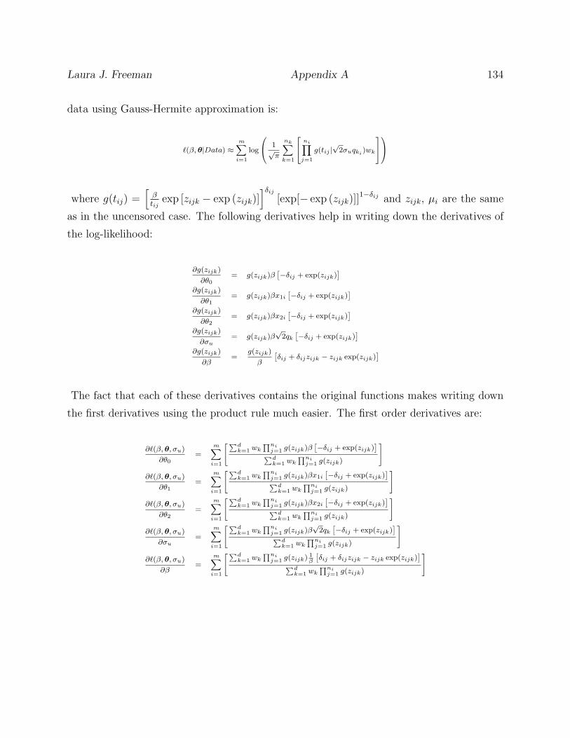
Laura J. Freeman Appendix A 134
data using Gauss-Hermite approximation is:
`(β,θ|Data) ≈m∑i=1
log
1√π
nk∑k=1
ni∏j=1
g(tij |√
2σuqki)wk
where g(tij) =[βtij
exp [zijk − exp (zijk)]]δij
[exp[− exp (zijk)]]1−δij and zijk, µi are the same
as in the uncensored case. The following derivatives help in writing down the derivatives of
the log-likelihood:
∂g(zijk)
∂θ0= g(zijk)β
[−δij + exp(zijk)
]∂g(zijk)
∂θ1= g(zijk)βx1i
[−δij + exp(zijk)
]∂g(zijk)
∂θ2= g(zijk)βx2i
[−δij + exp(zijk)
]∂g(zijk)
∂σu= g(zijk)β
√2qk
[−δij + exp(zijk)
]∂g(zijk)
∂β=
g(zijk)
β
[δij + δijzijk − zijk exp(zijk)
]
The fact that each of these derivatives contains the original functions makes writing down
the first derivatives using the product rule much easier. The first order derivatives are:
∂`(β,θ, σu)
∂θ0=
m∑i=1
[∑dk=1 wk
∏nij=1 g(zijk)β
[−δij + exp(zijk)
]∑dk=1 wk
∏nij=1 g(zijk)
]
∂`(β,θ, σu)
∂θ1=
m∑i=1
[∑dk=1 wk
∏nij=1 g(zijk)βx1i
[−δij + exp(zijk)
]∑dk=1 wk
∏nij=1 g(zijk)
]
∂`(β,θ, σu)
∂θ2=
m∑i=1
[∑dk=1 wk
∏nij=1 g(zijk)βx2i
[−δij + exp(zijk)
]∑dk=1 wk
∏nij=1 g(zijk)
]
∂`(β,θ, σu)
∂σu=
m∑i=1
[∑dk=1 wk
∏nij=1 g(zijk)β
√2qk
[−δij + exp(zijk)
]∑dk=1 wk
∏nij=1 g(zijk)
]
∂`(β,θ, σu)
∂β=
m∑i=1
[∑dk=1 wk
∏nij=1 g(zijk)
1β
[δij + δijzijk − zijk exp(zijk)
]∑dk=1 wk
∏nij=1 g(zijk)
]
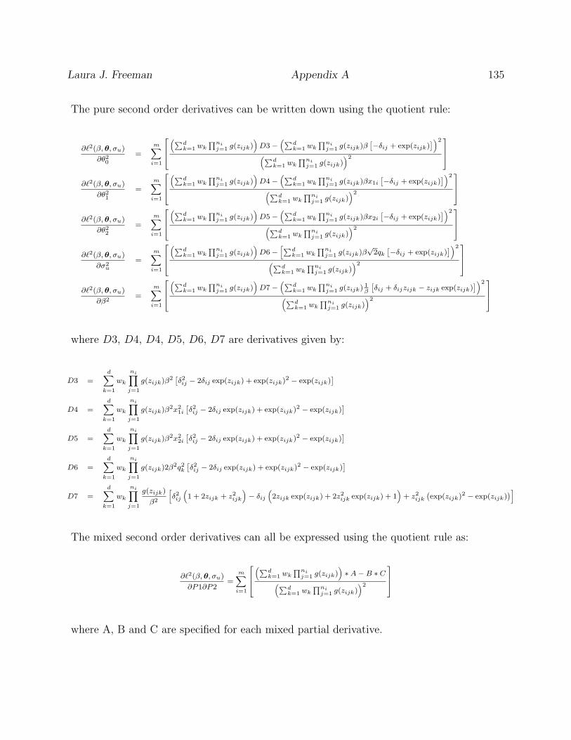
Laura J. Freeman Appendix A 135
The pure second order derivatives can be written down using the quotient rule:
∂`2(β,θ, σu)
∂θ20=
m∑i=1
(∑d
k=1 wk∏nij=1 g(zijk)
)D3−
(∑dk=1 wk
∏nij=1 g(zijk)β
[−δij + exp(zijk)
])2
(∑dk=1 wk
∏nij=1 g(zijk)
)2
∂`2(β,θ, σu)
∂θ21=
m∑i=1
(∑d
k=1 wk∏nij=1 g(zijk)
)D4−
(∑dk=1 wk
∏nij=1 g(zijk)βx1i
[−δij + exp(zijk)
])2
(∑dk=1 wk
∏nij=1 g(zijk)
)2
∂`2(β,θ, σu)
∂θ22=
m∑i=1
(∑d
k=1 wk∏nij=1 g(zijk)
)D5−
(∑dk=1 wk
∏nij=1 g(zijk)βx2i
[−δij + exp(zijk)
])2
(∑dk=1 wk
∏nij=1 g(zijk)
)2
∂`2(β,θ, σu)
∂σ2u
=
m∑i=1
(∑d
k=1 wk∏nij=1 g(zijk)
)D6−
[∑dk=1 wk
∏nij=1 g(zijk)β
√2qk
[−δij + exp(zijk)
])2
(∑dk=1 wk
∏nij=1 g(zijk)
)2
∂`2(β,θ, σu)
∂β2=
m∑i=1
(∑d
k=1 wk∏nij=1 g(zijk)
)D7−
(∑dk=1 wk
∏nij=1 g(zijk)
1β
[δij + δijzijk − zijk exp(zijk)
])2
(∑dk=1 wk
∏nij=1 g(zijk)
)2
where D3, D4, D4, D5, D6, D7 are derivatives given by:
D3 =d∑k=1
wk
ni∏j=1
g(zijk)β2[δ2ij − 2δij exp(zijk) + exp(zijk)
2 − exp(zijk)]
D4 =d∑k=1
wk
ni∏j=1
g(zijk)β2x2
1i
[δ2ij − 2δij exp(zijk) + exp(zijk)
2 − exp(zijk)]
D5 =
d∑k=1
wk
ni∏j=1
g(zijk)β2x2
2i
[δ2ij − 2δij exp(zijk) + exp(zijk)
2 − exp(zijk)]
D6 =
d∑k=1
wk
ni∏j=1
g(zijk)2β2q2k
[δ2ij − 2δij exp(zijk) + exp(zijk)
2 − exp(zijk)]
D7 =
d∑k=1
wk
ni∏j=1
g(zijk)
β2
[δ2ij
(1 + 2zijk + z2ijk
)− δij
(2zijk exp(zijk) + 2z2ijk exp(zijk) + 1
)+ z2ijk
(exp(zijk)
2 − exp(zijk))]
The mixed second order derivatives can all be expressed using the quotient rule as:
∂`2(β,θ, σu)
∂P1∂P2=
m∑i=1
(∑d
k=1 wk∏nij=1 g(zijk)
)∗A−B ∗ C(∑d
k=1 wk∏nij=1 g(zijk)
)2
where A, B and C are specified for each mixed partial derivative.

Laura J. Freeman Appendix A 136
For P1 = θ0 and P2 = θ1:
A =d∑k=1
wk
ni∏j=1
g(zijk)β2x1i
[δ2ij − 2δij exp(zijk) + exp(zijk)
2 − exp(zijk)]
B =
d∑k=1
wk
ni∏j=1
g(zijk)β[−δij + exp(zijk)
]
C =
d∑k=1
wk
ni∏j=1
g(zijk)βx1i
[−δij + exp(zijk)
]
For P1 = θ0 and P2 = θ2:
A =
d∑k=1
wk
ni∏j=1
g(zijk)β2x2i
[δ2ij − 2δij exp(zijk) + exp(zijk)
2 − exp(zijk)]
B =
d∑k=1
wk
ni∏j=1
g(zijk)β[−δij + exp(zijk)
]
C =
d∑k=1
wk
ni∏j=1
g(zijk)βx2i
[−δij + exp(zijk)
]
For P1 = θ0 and P2 = σu:
A =
d∑k=1
wk
ni∏j=1
g(zijk)β2√
2qk[δ2ij − 2δij exp(zijk) + exp(zijk)
2 − exp(zijk)]
B =
d∑k=1
wk
ni∏j=1
g(zijk)β[−δij + exp(zijk)
]
C =
d∑k=1
wk
ni∏j=1
g(zijk)β√
2qk[−δij + exp(zijk)
]
For P1 = θ0 and P2 = β:
A =
d∑k=1
wk
ni∏j=1
g(zijk)[(
exp(zijk)− δij) (δij + δijzijk − zijk exp(zijk)
)− δij + exp(zijk) + zijk exp(zijk)
]
B =
d∑k=1
wk
ni∏j=1
g(zijk)β[−δij + exp(zijk)
]
C =
d∑k=1
wk
ni∏j=1
g(zijk)1
β
[δij + δijzijk − zijk exp(zijk)
]

Laura J. Freeman Appendix A 137
For P1 = θ1 and P2 = θ2:
A =d∑k=1
wk
ni∏j=1
g(zijk)β2x1ix2i
[δ2ij − 2δij exp(zijk) + exp(zijk)
2 − exp(zijk)]
B =
d∑k=1
wk
ni∏j=1
g(zijk)βx1i
[−δij + exp(zijk)
]
C =
d∑k=1
wk
ni∏j=1
g(zijk)βx2i
[−δij + exp(zijk)
]
For P1 = θ1 and P2 = σu:
A =
d∑k=1
wk
ni∏j=1
g(zijk)β2x1i
√2qk
[δ2ij − 2δij exp(zijk) + exp(zijk)
2 − exp(zijk)]
B =
d∑k=1
wk
ni∏j=1
g(zijk)βx1i
[−δij + exp(zijk)
]
C =
d∑k=1
wk
ni∏j=1
g(zijk)β√
2qk[−δij + exp(zijk)
]
For P1 = θ1 and P2 = β:
A =d∑k=1
wk
ni∏j=1
g(zijk)[x1i
(exp(zijk)− δij
) (δij + δijzijk − zijk exp(zijk)
)+ x1i
(−δij + exp(zijk) + zijk exp(zijk)
)]
B =
d∑k=1
wk
ni∏j=1
g(zijk)βx1i
[−δij + exp(zijk)
]
C =
d∑k=1
wk
ni∏j=1
g(zijk)1
β
[δij + δijzijk − zijk exp(zijk)
]
For P1 = θ2 and P2 = σu:
A =
d∑k=1
wk
ni∏j=1
g(zijk)β2x2i
√2qk
[δ2ij − 2δij exp(zijk) + exp(zijk)
2 − exp(zijk)]
B =
d∑k=1
wk
ni∏j=1
g(zijk)βx2i
[−δij + exp(zijk)
]
C =d∑k=1
wk
ni∏j=1
g(zijk)β√
2qk[−δij + exp(zijk)
]

Laura J. Freeman Appendix A 138
For P1 = θ2 and P2 = β:
A =d∑k=1
wk
ni∏j=1
g(zijk)[x2i
(exp(zijk)− δij
) (δij + δijzijk − zijk exp(zijk)
)+ x2i
(−δij + exp(zijk) + zijk exp(zijk)
)]
B =
d∑k=1
wk
ni∏j=1
g(zijk)βx2i
[−δij + exp(zijk)
]
C =
d∑k=1
wk
ni∏j=1
g(zijk)1
β
[δij + δijzijk − zijk exp(zijk)
]
For P1 = σu and P2 = β:
A =
d∑k=1
wk
ni∏j=1
g(zijk)[√
2qk(exp(zijk)− δij
) (δij + δijzijk − zijk exp(zijk)
)+√
2qk(−δij + exp(zijk) + zijk exp(zijk)
)]
B =
d∑k=1
wk
ni∏j=1
g(zijk)β√
2qk[−δij + exp(zijk)
]
C =
d∑k=1
wk
ni∏j=1
g(zijk)1
β
[δij + δijzijk − zijk exp(zijk)
]
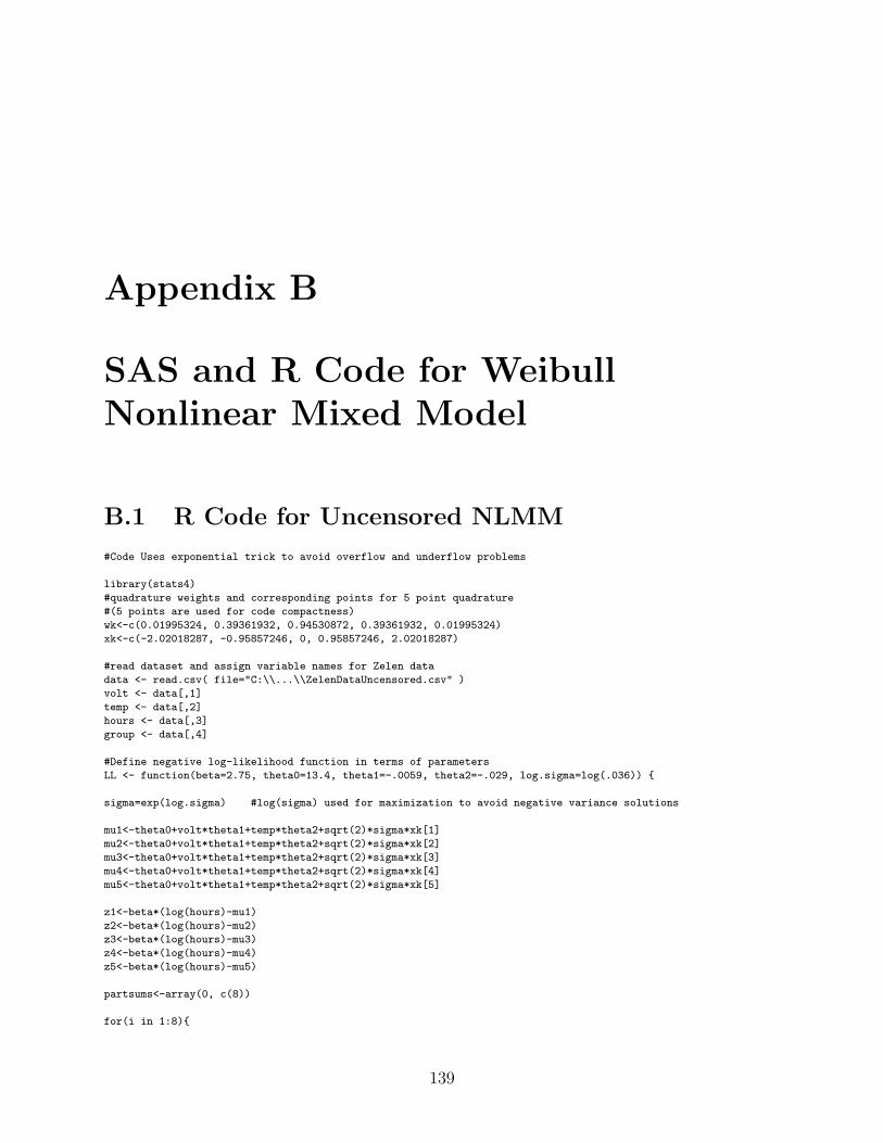
Appendix B
SAS and R Code for WeibullNonlinear Mixed Model
B.1 R Code for Uncensored NLMM
#Code Uses exponential trick to avoid overflow and underflow problems
library(stats4)
#quadrature weights and corresponding points for 5 point quadrature
#(5 points are used for code compactness)
wk<-c(0.01995324, 0.39361932, 0.94530872, 0.39361932, 0.01995324)
xk<-c(-2.02018287, -0.95857246, 0, 0.95857246, 2.02018287)
#read dataset and assign variable names for Zelen data
data <- read.csv( file="C:\\...\\ZelenDataUncensored.csv" )
volt <- data[,1]
temp <- data[,2]
hours <- data[,3]
group <- data[,4]
#Define negative log-likelihood function in terms of parameters
LL <- function(beta=2.75, theta0=13.4, theta1=-.0059, theta2=-.029, log.sigma=log(.036)) {
sigma=exp(log.sigma) #log(sigma) used for maximization to avoid negative variance solutions
mu1<-theta0+volt*theta1+temp*theta2+sqrt(2)*sigma*xk[1]
mu2<-theta0+volt*theta1+temp*theta2+sqrt(2)*sigma*xk[2]
mu3<-theta0+volt*theta1+temp*theta2+sqrt(2)*sigma*xk[3]
mu4<-theta0+volt*theta1+temp*theta2+sqrt(2)*sigma*xk[4]
mu5<-theta0+volt*theta1+temp*theta2+sqrt(2)*sigma*xk[5]
z1<-beta*(log(hours)-mu1)
z2<-beta*(log(hours)-mu2)
z3<-beta*(log(hours)-mu3)
z4<-beta*(log(hours)-mu4)
z5<-beta*(log(hours)-mu5)
partsums<-array(0, c(8))
for(i in 1:8){
139

Laura J. Freeman Appendix B 140
e11<-sum(z1[((i-1)*4):(4*i)]-exp(z1[((i-1)*4):(4*i)]))
e12<-sum(z2[((i-1)*4):(4*i)]-exp(z2[((i-1)*4):(4*i)]))
e13<-sum(z3[((i-1)*4):(4*i)]-exp(z3[((i-1)*4):(4*i)]))
e14<-sum(z4[((i-1)*4):(4*i)]-exp(z4[((i-1)*4):(4*i)]))
e15<-sum(z5[((i-1)*4):(4*i)]-exp(z5[((i-1)*4):(4*i)]))
maxabs <- max(abs(e11), abs(e12), abs(e13), abs(e14), abs(e15))
maxnorm <- max(e11, e12, e13, e14, e15)
if (maxabs > maxnorm) c1 <- min(e11, e12, e13, e14, e15) else c1 <- maxnorm
h11 <- wk[1]/sqrt(pi)*exp(e11-c1)
h12 <- wk[2]/sqrt(pi)*exp(e12-c1)
h13 <- wk[3]/sqrt(pi)*exp(e13-c1)
h14 <- wk[4]/sqrt(pi)*exp(e14-c1)
h15 <- wk[5]/sqrt(pi)*exp(e15-c1)
h1 <- c(h11, h12, h13, h14, h15)
partsums[i] <- log(beta^4/(prod(hours[((i-1)*4):(4*i)])))+log(sum(h1))+c1
}
return(-(sum(partsums))) #Return negative log-likelihood
}
#Find MLEs using built in R - function
#mle() uses numerical derivatives - can be problematic
fit<-mle(LL,start=list(beta=3.617, theta0=13.1534, theta1=-.00626, theta2=-.02904,
log.sigma=log(.155)), method="BFGS", control=list(trace))
summary(fit) #print fit summary
vcov(fit) #store covariance estimate from mle function
#Hessian Calculations
#set values for hessian calculations to MLEs from above
beta<-coef(fit)[1]; theta0<-coef(fit)[1]; theta1<-coef(fit)[1]; theta2<-coef(fit)[1];
log.sigma<-coef(fit)[1];
sigma=exp(log.sigma)
mu1<-theta0+volt*theta1+temp*theta2+sqrt(2)*sigma*xk[1]
mu2<-theta0+volt*theta1+temp*theta2+sqrt(2)*sigma*xk[2]
mu3<-theta0+volt*theta1+temp*theta2+sqrt(2)*sigma*xk[3]
mu4<-theta0+volt*theta1+temp*theta2+sqrt(2)*sigma*xk[4]
mu5<-theta0+volt*theta1+temp*theta2+sqrt(2)*sigma*xk[5]
z1<-beta*(log(hours)-mu1)
z2<-beta*(log(hours)-mu2)
z3<-beta*(log(hours)-mu3)
z4<-beta*(log(hours)-mu4)
z5<-beta*(log(hours)-mu5)
z<-cbind(z1,z2,z3,z4,z5) #create matrix of z-values
H=matrix(0,5,5) #create empty Hessian matrix
#create vectors to store sums for each calculation
sums<-array(0, c(5, 23, 8))
der22<-array(0, c(8))
der23<-array(0, c(8))
der24<-array(0, c(8))

Laura J. Freeman Appendix B 141
der25<-array(0, c(8))
der21<-array(0, c(8))
der33<-array(0, c(8))
der34<-array(0, c(8))
der35<-array(0, c(8))
der31<-array(0, c(8))
der44<-array(0, c(8))
der45<-array(0, c(8))
der41<-array(0, c(8))
der55<-array(0, c(8))
der51<-array(0, c(8))
der11<-array(0, c(8))
for(i in 1:8){
bottom<-0;
top2<-0; dtop22<-0; dbottom22<-0; dtop23<-0; dbottom23<-0; dtop24<-0; dbottom24<-0;
dtop25<-0; dbottom25<-0; dtop21<-0; dbottom21<-0;
top3<-0; dtop33<-0; dbottom33<-0; dtop34<-0; dbottom34<-0; dtop35<-0; dbottom35<-0;
dtop31<-0; dbottom31<-0;
top4<-0; dtop44<-0; dbottom44<-0; dtop45<-0; dbottom45<-0; dtop41<-0; dbottom41<-0;
top5<-0; dtop55<-0; dbottom55<-0; dtop51<-0; dbottom51<-0;
top1<-0; dtop11<-0; dbottom11<-0;
for(k in 1:5){
print(i);
sums[k,1,i]<-exp(sum(z[((i-1)*4+1):(i*4),k]-exp(z[((i-1)*4+1):(i*4),k])));
sums[k,2,i]<-sum(-beta+beta*exp(z[((i-1)*4+1):(i*4),k]));
sums[k,3,i]<-sum(-beta^2*exp(z[((i-1)*4+1):(i*4),k]));
sums[k,4,i]<-sum(-beta*volt[((i-1)*4+1):(i*4)]+
beta*volt[((i-1)*4+1):(i*4)]*exp(z[((i-1)*4+1):(i*4),k]));
sums[k,5,i]<-sum(-beta^2*volt[((i-1)*4+1):(i*4)]*exp(z[((i-1)*4+1):(i*4),k]));
sums[k,6,i]<-sum(-beta*sqrt(2)*xk[k]+beta*sqrt(2)*xk[k]*exp(z[((i-1)*4+1):(i*4),k]));
sums[k,7,i]<-sum(-2*(xk[k]*beta)^2*exp(z[((i-1)*4+1):(i*4),k]));
sums[k,8,i]<-sum(z[((i-1)*4+1):(i*4),k]/beta-z[((i-1)*4+1):(i*4),k]/beta
*exp(z[((i-1)*4+1):(i*4),k]));
sums[k,9,i]<-sum(-sqrt(2)*xk[k]+sqrt(2)*xk[k]*exp(z[((i-1)*4+1):(i*4),k])+
sqrt(2)*xk[k]*z[((i-1)*4+1):(i*4),k]*exp(z[((i-1)*4+1):(i*4),k]));
sums[k,10,i]<-sum(-(beta*volt[((i-1)*4+1):(i*4)])^2*exp(z[((i-1)*4+1):(i*4),k]));
sums[k,11,i]<-sum(-beta*temp[((i-1)*4+1):(i*4)]+beta*temp[((i-1)*4+1):(i*4)]
*exp(z[((i-1)*4+1):(i*4),k]));
sums[k,12,i]<-sum(-beta^2*temp[((i-1)*4+1):(i*4)]*exp(z[((i-1)*4+1):(i*4),k]));
sums[k,13,i]<-sum(-sqrt(2)*xk[k]*beta^2*exp(z[((i-1)*4+1):(i*4),k]));
sums[k,14,i]<-sum(-1+exp(z[((i-1)*4+1):(i*4),k])+z[((i-1)*4+1):(i*4),k]
*exp(z[((i-1)*4+1):(i*4),k]));
sums[k,15,i]<-sum(-beta^2*volt[((i-1)*4+1):(i*4)]*temp[((i-1)*4+1):(i*4)]
*exp(z[((i-1)*4+1):(i*4),k]));
sums[k,16,i]<-sum(-sqrt(2)*xk[k]*beta^2*volt[((i-1)*4+1):(i*4)]*exp(z[((i-1)*4+1):(i*4),k]));
sums[k,17,i]<-sum(-volt[((i-1)*4+1):(i*4)]+volt[((i-1)*4+1):(i*4)]*exp(z[((i-1)*4+1):(i*4),k])+
volt[((i-1)*4+1):(i*4)]*z[((i-1)*4+1):(i*4),k]*exp(z[((i-1)*4+1):(i*4),k]));
sums[k,18,i]<-sum(-beta^2*temp[((i-1)*4+1):(i*4)]*temp[((i-1)*4+1):(i*4)]
*exp(z[((i-1)*4+1):(i*4),k]));
sums[k,19,i]<-sum(-sqrt(2)*xk[k]*beta^2*temp[((i-1)*4+1):(i*4)]*exp(z[((i-1)*4+1):(i*4),k]));
sums[k,20,i]<-sum(-temp[((i-1)*4+1):(i*4)]+temp[((i-1)*4+1):(i*4)]*exp(z[((i-1)*4+1):(i*4),k])+
temp[((i-1)*4+1):(i*4)]*z[((i-1)*4+1):(i*4),k]*exp(z[((i-1)*4+1):(i*4),k]));
sums[k,21,i]<-sum((z[((i-1)*4+1):(i*4),k]/beta)^2*exp(z[((i-1)*4+1):(i*4),k]));
sums[k,22,i]<-sum((z[((i-1)*4+1):(i*4),k]/beta));
sums[k,23,i]<-sum((z[((i-1)*4+1):(i*4),k]/beta)*exp(z[((i-1)*4+1):(i*4),k]));

Laura J. Freeman Appendix B 142
bottom<-bottom+wk[k]*sums[k,1,i];
top2<-top2+wk[k]*sums[k,1,i]*sums[k,2,i];
dtop22<-dtop22+wk[k]*(sums[k,1,i]*sums[k,3,i]+sums[k,1,i]*sums[k,2,i]^2);
dbottom22<-dbottom22+wk[k]*sums[k,1,i]*sums[k,2,i];
dtop23<-dtop23+wk[k]*(sums[k,1,i]*sums[k,5,i]+sums[k,1,i]*sums[k,4,i]*sums[k,2,i]);
dbottom23<-dbottom23+wk[k]*sums[k,1,i]*sums[k,4,i];
dtop24<-dtop24+wk[k]*(sums[k,1,i]*sums[k,12,i]+sums[k,1,i]*sums[k,11,i]*sums[k,2,i]);
dbottom24<-dbottom24+wk[k]*sums[k,1,i]*sums[k,11,i];
dtop25<-dtop25+wk[k]*(sums[k,1,i]*sums[k,13,i]+sums[k,1,i]*sums[k,6,i]*sums[k,2,i]);
dbottom25<-dbottom25+wk[k]*sums[k,1,i]*sums[k,6,i];
dtop21<-dtop21+wk[k]*(sums[k,1,i]*sums[k,14,i]+sums[k,1,i]*sums[k,8,i]*sums[k,2,i]);
dbottom21<-dbottom21+wk[k]*sums[k,1,i]*sums[k,8,i];
top3<-top3+wk[k]*sums[k,1,i]*sums[k,4,i];
dtop33<-dtop33+wk[k]*(sums[k,1,i]*sums[k,10,i]+sums[k,1,i]*sums[k,4,i]^2);
dbottom33<-dbottom33+wk[k]*sums[k,1,i]*sums[k,4,i];
dtop34<-dtop34+wk[k]*(sums[k,1,i]*sums[k,15,i]+sums[k,1,i]*sums[k,11,i]*sums[k,4,i]);
dbottom34<-dbottom34+wk[k]*sums[k,1,i]*sums[k,11,i];
dtop35<-dtop35+wk[k]*(sums[k,1,i]*sums[k,16,i]+sums[k,1,i]*sums[k,6,i]*sums[k,4,i]);
dbottom35<-dbottom35+wk[k]*sums[k,1,i]*sums[k,6,i];
dtop31<-dtop31+wk[k]*(sums[k,1,i]*sums[k,17,i]+sums[k,1,i]*sums[k,8,i]*sums[k,4,i]);
dbottom31<-dbottom31+wk[k]*sums[k,1,i]*sums[k,8,i];
top4<-top4+wk[k]*sums[k,1,i]*sums[k,11,i];
dtop44<-dtop44+wk[k]*(sums[k,1,i]*sums[k,18,i]+sums[k,1,i]*sums[k,11,i]^2);
dbottom44<-dbottom44+wk[k]*sums[k,1,i]*sums[k,11,i];
dtop45<-dtop45+wk[k]*(sums[k,1,i]*sums[k,19,i]+sums[k,1,i]*sums[k,6,i]*sums[k,11,i]);
dbottom45<-dbottom45+wk[k]*sums[k,1,i]*sums[k,6,i];
dtop41<-dtop41+wk[k]*(sums[k,1,i]*sums[k,20,i]+sums[k,1,i]*sums[k,8,i]*sums[k,11,i]);
dbottom41<-dbottom41+wk[k]*sums[k,1,i]*sums[k,8,i];
top5<-top5+wk[k]*sums[k,1,i]*sums[k,6,i];
dtop55<-dtop55+wk[k]*(sums[k,1,i]*sums[k,7,i]+sums[k,1,i]*sums[k,6,i]^2)
dbottom55<-dbottom55+wk[k]*sums[k,1,i]*sums[k,6,i]
dtop51<-dtop51+wk[k]*(sums[k,1,i]*sums[k,9,i]+sums[k,1,i]*sums[k,8,i]*sums[k,6,i]);
dbottom51<-dbottom51+wk[k]*sums[k,1,i]*sums[k,8,i];
ni<-4
top1<-top1+ni*wk[k]*sums[k,1,i]+beta*wk[k]*sums[k,1,i]*sums[k,8,i]
dtop11<-dtop11+(ni+1)*wk[k]*sums[k,1,i]*sums[k,8,i]+beta*wk[k]*sums[k,1,i]*sums[k,8,i]*sums[k,22,i]
-beta*wk[k]*sums[k,1,i]*sums[k,8,i]*sums[k,23,i]-beta*wk[k]*sums[k,1,i]*sums[k,21,i]
dbottom11<-dbottom11+wk[k]*sums[k,1,i]+beta*wk[k]*sums[k,1,i]*sums[k,8,i]
}
der22[i]<-(bottom*dtop22-top2*dbottom22)/(bottom^2)
der23[i]<-(bottom*dtop23-top2*dbottom23)/(bottom^2)
der24[i]<-(bottom*dtop24-top2*dbottom24)/(bottom^2)
der25[i]<-(bottom*dtop25-top2*dbottom25)/(bottom^2)
der21[i]<-(bottom*dtop21-top2*dbottom21)/(bottom^2)
der33[i]<-(bottom*dtop33-top3*dbottom33)/(bottom^2)
der34[i]<-(bottom*dtop34-top3*dbottom34)/(bottom^2)

Laura J. Freeman Appendix B 143
der35[i]<-(bottom*dtop35-top3*dbottom35)/(bottom^2)
der31[i]<-(bottom*dtop31-top3*dbottom31)/(bottom^2)
der44[i]<-(bottom*dtop44-top4*dbottom44)/(bottom^2)
der45[i]<-(bottom*dtop45-top4*dbottom45)/(bottom^2)
der41[i]<-(bottom*dtop41-top4*dbottom41)/(bottom^2)
der55[i]<-(bottom*dtop55-top5*dbottom55)/(bottom^2)
der51[i]<-(bottom*dtop51-top5*dbottom51)/(bottom^2)
der11[i]<-(beta*bottom*dtop11-top1*dbottom11)/(beta*bottom)^2
}
H[1,1]<--sum(der11)
H[1,2]<--sum(der21); H[2,1]<--sum(der21)
H[1,3]<--sum(der31); H[3,1]<--sum(der31)
H[1,4]<--sum(der41); H[4,1]<--sum(der41)
H[1,5]<--sum(der51); H[5,1]<--sum(der51)
H[2,2]<--sum(der22)
H[2,3]<--sum(der23); H[3,2]<--sum(der23)
H[2,4]<--sum(der24); H[4,2]<--sum(der24)
H[2,5]<--sum(der25); H[5,2]<--sum(der25)
H[3,3]<--sum(der33)
H[3,4]<--sum(der34); H[4,3]<--sum(der34)
H[3,5]<--sum(der35); H[5,3]<--sum(der35)
H[4,4]<--sum(der44)
H[4,5]<--sum(der45); H[5,4]<--sum(der45)
H[5,5]<--sum(der55)
print(H) #output Hessian matrix
B.2 R Code for Censored NLMM
#Censored Weibull with log sum of exponentials rules
library(stats4)
wk<-c(0.01995324, 0.39361932, 0.94530872, 0.39361932, 0.01995324)
xk<-c(-2.02018287, -0.95857246, 0, 0.95857246, 2.02018287)
data <- read.csv( file="C:\\...\\ZelenData.csv" )
volt <- data[,1]
temp <- data[,2]
hours <- data[,3]
group <- data[,4]
delta <- data[,5]
LL <- function(beta=2.75,theta0=13.4,theta1=-.0059,theta2=-.029,log.sigma=log(.036)){
#negative log-likelihood function
sigma=exp(log.sigma)
mu1<-theta0+volt*theta1+temp*theta2+sqrt(2)*sigma*xk[1]
mu2<-theta0+volt*theta1+temp*theta2+sqrt(2)*sigma*xk[2]
mu3<-theta0+volt*theta1+temp*theta2+sqrt(2)*sigma*xk[3]
mu4<-theta0+volt*theta1+temp*theta2+sqrt(2)*sigma*xk[4]
mu5<-theta0+volt*theta1+temp*theta2+sqrt(2)*sigma*xk[5]
z1<-beta*(log(hours)-mu1)
z2<-beta*(log(hours)-mu2)
z3<-beta*(log(hours)-mu3)
z4<-beta*(log(hours)-mu4)

Laura J. Freeman Appendix B 144
z5<-beta*(log(hours)-mu5)
partsums<-array(0, c(8))
for(i in 1:8){
e11<-sum(z1[((i-1)*4):(4*i)]-exp(z1[((i-1)*4):(4*i)]))
e12<-sum(z2[((i-1)*4):(4*i)]-exp(z2[((i-1)*4):(4*i)]))
e13<-sum(z3[((i-1)*4):(4*i)]-exp(z3[((i-1)*4):(4*i)]))
e14<-sum(z4[((i-1)*4):(4*i)]-exp(z4[((i-1)*4):(4*i)]))
e15<-sum(z5[((i-1)*4):(4*i)]-exp(z5[((i-1)*4):(4*i)]))
maxabs <- max(abs(e11), abs(e12), abs(e13), abs(e14), abs(e15))
maxnorm <- max(e11, e12, e13, e14, e15)
if (maxabs > maxnorm) c1 <- min(e11, e12, e13, e14, e15) else c1 <- maxnorm
h11 <- wk[1]/sqrt(pi)*exp(e11-c1)
h12 <- wk[2]/sqrt(pi)*exp(e12-c1)
h13 <- wk[3]/sqrt(pi)*exp(e13-c1)
h14 <- wk[4]/sqrt(pi)*exp(e14-c1)
h15 <- wk[5]/sqrt(pi)*exp(e15-c1)
h1 <- c(h11, h12, h13, h14, h15)
partsums[i] <- log(beta^4/(prod(hours[((i-1)*4):(4*i)])))+log(sum(h1))+c1
}
return(-(sum(partsums)))
}
fit<-mle(LL,start=list(beta=3.617, theta0=13.1534, theta1=-.00626, theta2=-.02904,
log.sigma=log(.155)), method="BFGS", control=list(trace))
summary(fit)
vcov(fit5)
#Hessian Calculations are done similarly to uncensored case and are omitted
B.3 SAS Code for Censored NLMM
proc nlmixed data=work.data method=gauss noad noadscale QPOINTS=20 tech=quanew
update=bfgs cov;
parms beta=2.78 theta0=6.7 theta1=-.44 logsigma=-3;
z = beta*(log(t)-theta0-theta1*volt - u);
f1= beta/t*exp(z-exp(z));
F2=exp(-exp(z));
ll=log(f1)*(Censored=0)+log(F2)*(Censored=1);
sigma2=exp(logsigma)**2;
model t ~general(ll);
random u ~ normal(0, sigma2) subject=group;
ods output ParameterEstimates=mydata.parmest;
run;

Laura J. Freeman Appendix B 145
B.4 SAS Code for Random Effect Bootstrapping in
NLMM
*Construct Resampled data------------------------------------------------------------;
proc sort data=work.ZELENCENSORED;
by group;
run;
proc surveyselect data=work.ZELENCENSORED method=URS n=8 out=sample1 rep=10000 outhits;
strata group;
run;
proc sort data=work.sample1;
by Replicate;
run;
proc nlmixed data=work.sample1 method=gauss noad noadscale QPOINTS=20 tech=quanew
update=bfgs cov;
by Replicate;
parms beta=2.78 theta0=6.7 theta1=-.44 theta2=-.44 logsigma=-1.2;
z = beta*(log(hours)-theta0-theta1*voltcode-theta2*tempcode - u);
f1= beta*exp(z-exp(z));
F2=exp(-exp(z));
ll=log(f1)*(Censored=0)+log(F2)*(Censored=1);
sigma2=(exp(logsigma))**2;
model hours ~general(ll);
random u ~ normal(0, sigma2) subject=group;
ods output FitStatistics=work.loglikesample1;
run;
proc lifereg data=work.sample1;
by replicate;
model hours*Censored(1)=voltcode tempcode;
ods output ModelInfo=work.loglikesample1null;
run;
data work.loglikesample1;
set work.loglikesample1;
where Descr=’-2 Log Likelihood’;
model=’alt’;
altvalue=value;
drop value;
run;
data work.loglikesample1null;
set work.loglikesample1null;
where Label1=’Log Likelihood’;
model=’null’;
run;
data work.LRTsample1;
merge work.loglikesample1null work.loglikesample1;
by Replicate;
if altvalue = . then delete;
if cvalue1 = . then delete;
LRT=-2*cvalue1-altvalue;
run;

Laura J. Freeman Appendix B 146
proc means data=work.lrtsample1 n;
var Replicate;
ods output Summary = work.replicatesize;
run;
data work.lrtdata;
merge work.lrtdata work.replicatesize;
run;
data work.test;
retain rep replicate teststat;
set work.lrtdata;
n = replicate_n;
do replicate = 1 to n;
rawteststat=LRT;
output;
end;
drop LRT replicate_n;
run;
data work.pvalue;
merge work.lrtsample1 work.test;
count=LRT>=rawteststat;
run;
proc means data=work.pvalue n mean;
var count;
ods output summary = work.pvalues;
run;