Embed Size (px)
Citation preview

STATISTICAL METHODS FOR SIGNAL PROCESSING
Alfred O. Hero
December 19, 2006
This set of notes is the primary source material for the course EECS564 “Estimation, filtering anddetection” used over the period 1999-2006 at the University of Michigan Ann Arbor. The authorcan be reached atDept. EECS, University of Michigan, Ann Arbor, MI 48109-2122Tel: 734-763-0564.email [email protected];http://www.eecs.umich.edu/~hero/.
1

STATISTICAL METHODS FOR SIGNAL PROCESSING c©Alfred Hero 1999 2
Contents
1 INTRODUCTION 9
1.1 STATISTICAL SIGNAL PROCESSING . . . . . . . . . . . . . . . . . . . . . . . 9
1.2 PERSPECTIVE ADOPTED IN THIS BOOK . . . . . . . . . . . . . . . . . . . 9
1.2.1 PREREQUISITES . . . . . . . . . . . . . . . . . . . . . . . . . . . . . . . 11
2 NOTATION, MATRIX ALGEBRA, SIGNALS AND SYSTEMS 12
2.1 NOTATION . . . . . . . . . . . . . . . . . . . . . . . . . . . . . . . . . . . . . . 12
2.2 VECTOR AND MATRIX BACKGROUND . . . . . . . . . . . . . . . . . . . . . 12
2.2.1 ROW AND COLUMN VECTORS . . . . . . . . . . . . . . . . . . . . . . 12
2.2.2 VECTOR/VECTOR MULTIPLICATION . . . . . . . . . . . . . . . . . 13
2.3 ORTHOGONAL VECTORS . . . . . . . . . . . . . . . . . . . . . . . . . . . . . 13
2.3.1 VECTOR/MATRIX MULTIPLICATION . . . . . . . . . . . . . . . . . . 14
2.3.2 THE LINEAR SPAN OF A SET OF VECTORS . . . . . . . . . . . . . . 14
2.3.3 RANK OF A MATRIX . . . . . . . . . . . . . . . . . . . . . . . . . . . . 14
2.3.4 MATRIX INVERSION . . . . . . . . . . . . . . . . . . . . . . . . . . . . 14
2.3.5 ORTHOGONAL AND UNITARY MATRICES . . . . . . . . . . . . . . . 15
2.3.6 GRAMM-SCHMIDT ORTHOGONALIZATION AND ORTHONORMAL-IZATION . . . . . . . . . . . . . . . . . . . . . . . . . . . . . . . . . . . . . 15
2.3.7 EIGENVALUES OF A SYMMETRIC MATRIX . . . . . . . . . . . . . . 16
2.3.8 MATRIX DIAGONALIZATION AND EIGENDECOMPOSITION . . . . 16
2.3.9 QUADRATIC FORMS AND NON-NEGATIVE DEFINITE MATRICES 17
2.4 POSITIVE DEFINITENESS OF SYMMETRIC PARTITIONED MATRICES . 17
2.4.1 DETERMINANT OF A MATRIX . . . . . . . . . . . . . . . . . . . . . . 18
2.4.2 TRACE OF A MATRIX . . . . . . . . . . . . . . . . . . . . . . . . . . . 18
2.4.3 VECTOR DIFFERENTIATION . . . . . . . . . . . . . . . . . . . . . . . 18
2.5 SIGNALS AND SYSTEMS BACKGROUND . . . . . . . . . . . . . . . . . . . . 19
2.5.1 GEOMETRIC SERIES . . . . . . . . . . . . . . . . . . . . . . . . . . . . 19
2.5.2 LAPLACE AND FOURIER TRANSFORMS OF FUNCTIONS OF ACONTINUOUS VARIABLE . . . . . . . . . . . . . . . . . . . . . . . . . . 19
2.5.3 Z-TRANSFORM AND DISCRETE-TIME FOURIER TRANSFORM (DTFT) 19
2.5.4 CONVOLUTION: CONTINUOUS TIME . . . . . . . . . . . . . . . . . . 20
2.5.5 CONVOLUTION: DISCRETE TIME . . . . . . . . . . . . . . . . . . . . 20
2.5.6 CORRELATION: DISCRETE TIME . . . . . . . . . . . . . . . . . . . . 21
2.5.7 RELATION BETWEEN CORRELATION AND CONVOLUTION . . . 21
2.5.8 CONVOLUTION AS A MATRIX OPERATION . . . . . . . . . . . . . . 21
2.6 BACKGROUND REFERENCES . . . . . . . . . . . . . . . . . . . . . . . . . . . 21
2.7 EXERCISES . . . . . . . . . . . . . . . . . . . . . . . . . . . . . . . . . . . . . . . 22

STATISTICAL METHODS FOR SIGNAL PROCESSING c©Alfred Hero 1999 3
3 STATISTICAL MODELS 24
3.1 THE GAUSSIAN DISTRIBUTION AND ITS RELATIVES . . . . . . . . . . . . 24
3.1.1 CHI-SQUARE . . . . . . . . . . . . . . . . . . . . . . . . . . . . . . . . . 26
3.1.2 GAMMA . . . . . . . . . . . . . . . . . . . . . . . . . . . . . . . . . . . . 27
3.1.3 NON-CENTRAL CHI SQUARE . . . . . . . . . . . . . . . . . . . . . . . 27
3.1.4 CHI-SQUARE MIXTURE . . . . . . . . . . . . . . . . . . . . . . . . . . 28
3.1.5 STUDENT-T . . . . . . . . . . . . . . . . . . . . . . . . . . . . . . . . . . 28
3.1.6 FISHER-F . . . . . . . . . . . . . . . . . . . . . . . . . . . . . . . . . . . 28
3.1.7 CAUCHY . . . . . . . . . . . . . . . . . . . . . . . . . . . . . . . . . . . . 29
3.1.8 BETA . . . . . . . . . . . . . . . . . . . . . . . . . . . . . . . . . . . . . . 29
3.2 REPRODUCING DISTRIBUTIONS . . . . . . . . . . . . . . . . . . . . . . . . . 29
3.3 FISHER-COCHRAN THEOREM . . . . . . . . . . . . . . . . . . . . . . . . . . 30
3.4 SAMPLE MEAN AND SAMPLE VARIANCE . . . . . . . . . . . . . . . . . . . 30
3.5 SUFFICIENT STATISTICS . . . . . . . . . . . . . . . . . . . . . . . . . . . . . 32
3.5.1 SUFFICIENT STATISTICS AND THE REDUCTION RATIO . . . . . . 33
3.5.2 DEFINITION OF SUFFICIENCY . . . . . . . . . . . . . . . . . . . . . . 34
3.5.3 MINIMAL SUFFICIENCY . . . . . . . . . . . . . . . . . . . . . . . . . . 36
3.5.4 EXPONENTIAL FAMILY OF DISTRIBUTIONS . . . . . . . . . . . . . 39
3.5.5 CHECKING IF A DENSITY IS IN THE EXPONENTIAL FAMILY . . 40
3.6 BACKGROUND REFERENCES . . . . . . . . . . . . . . . . . . . . . . . . . . . 41
3.7 EXERCISES . . . . . . . . . . . . . . . . . . . . . . . . . . . . . . . . . . . . . . . 41
4 FUNDAMENTALS OF PARAMETRIC ESTIMATION 43
4.1 ESTIMATION: MAIN INGREDIENTS . . . . . . . . . . . . . . . . . . . . . . . 43
4.2 ESTIMATION OF RANDOM SCALAR PARAMETERS . . . . . . . . . . . . . 44
4.2.1 MINIMUM MEAN SQUARED ERROR ESTIMATION . . . . . . . . . . 45
4.2.2 MINIMUM MEAN ABSOLUTE ERROR ESTIMATOR . . . . . . . . . 47
4.2.3 MINIMUM MEAN UNIFORM ERROR ESTIMATION . . . . . . . . . . 48
4.2.4 BAYES ESTIMATOR EXAMPLES . . . . . . . . . . . . . . . . . . . . . 50
4.3 ESTIMATION OF RANDOM VECTOR VALUED PARAMETERS . . . . . . . 60
4.3.1 VECTOR SQUARED ERROR . . . . . . . . . . . . . . . . . . . . . . . . 61
4.3.2 VECTOR UNIFORM ERROR . . . . . . . . . . . . . . . . . . . . . . . . 61
4.4 ESTIMATION OF NON-RANDOM PARAMETERS . . . . . . . . . . . . . . . 64
4.4.1 SCALAR ESTIMATION CRITERIA FOR NON-RANDOM PARAME-TERS . . . . . . . . . . . . . . . . . . . . . . . . . . . . . . . . . . . . . . . 64
4.4.2 METHOD OF MOMENTS (MOM) SCALAR ESTIMATORS . . . . . . 67
4.4.3 MAXIMUM LIKELIHOOD (ML) SCALAR ESTIMATORS . . . . . . . 71
STATISTICAL METHODS FOR SIGNAL PROCESSING c©Alfred Hero 1999 4
4.4.4 SCALAR CRAMER-RAO BOUND (CRB) ON ESTIMATOR VARIANCE 74
4.5 ESTIMATION OF MULTIPLE NON-RANDOM PARAMETERS . . . . . . . . 80
4.5.1 MATRIX CRAMER-RAO BOUND (CRB) ON COVARIANCE MATRIX 81
4.5.2 METHODS OF MOMENTS (MOM) VECTOR ESTIMATION . . . . . 85
4.5.3 MAXIMUM LIKELIHOOD (ML) VECTOR ESTIMATION . . . . . . . 85
4.6 HANDLING NUISANCE PARAMETERS . . . . . . . . . . . . . . . . . . . . . 89
4.7 BACKGROUND REFERENCES . . . . . . . . . . . . . . . . . . . . . . . . . . . 91
4.8 EXERCISES . . . . . . . . . . . . . . . . . . . . . . . . . . . . . . . . . . . . . . . 92
5 LINEAR ESTIMATION 101
5.1 MIN MSE CONSTANT, LINEAR, AND AFFINE ESTIMATION . . . . . . . . 101
5.1.1 BEST CONSTANT ESTIMATOR OF A SCALAR RANDOM PARAME-TER . . . . . . . . . . . . . . . . . . . . . . . . . . . . . . . . . . . . . . . . 102
5.2 BEST LINEAR ESTIMATOR OF A SCALAR RANDOM PARAMETER . . . 102
5.3 BEST AFFINE ESTIMATOR OF A SCALAR R.V. θ . . . . . . . . . . . . . . . 103
5.3.1 SUPERPOSITION PROPERTY OF LINEAR/AFFINE ESTIMATORS 105
5.4 GEOMETRIC INTERPRETATION: ORTHOGONALITY CONDITION ANDPROJECTION THEOREM . . . . . . . . . . . . . . . . . . . . . . . . . . . . . . . 105
5.4.1 LINEAR MINIMUM MSE ESTIMATION REVISITED . . . . . . . . . . 105
5.4.2 AFFINE MINIMUM MSE ESTIMATION . . . . . . . . . . . . . . . . . 107
5.4.3 OPTIMALITY OF AFFINE ESTIMATOR FOR LINEAR GAUSSIANMODEL . . . . . . . . . . . . . . . . . . . . . . . . . . . . . . . . . . . . . . 107
5.5 BEST AFFINE ESTIMATION OF A VECTOR . . . . . . . . . . . . . . . . . . 108
5.5.1 LINEAR ESTIMATION EXAMPLES . . . . . . . . . . . . . . . . . . . . 109
5.6 NONSTATISTICAL LEAST SQUARES (LINEAR REGRESSION) . . . . . . . 111
5.7 LINEAR MINIMUM WEIGHTED LEAST SQUARES ESTIMATION . . . . . . 118
5.7.1 PROJECTION OPERATOR FORM OF LMWLS PREDICTOR . . . . . 118
5.8 OPTIMALITY OF LMWMS IN THE GAUSSIAN MODEL . . . . . . . . . . . 121
5.9 BACKGROUND REFERENCES . . . . . . . . . . . . . . . . . . . . . . . . . . . 123
5.10 APPENDIX: VECTOR SPACES . . . . . . . . . . . . . . . . . . . . . . . . . . . 123
5.11 EXERCISES . . . . . . . . . . . . . . . . . . . . . . . . . . . . . . . . . . . . . . . 127
6 OPTIMAL LINEAR FILTERING AND PREDICTION 132
6.1 WIENER-HOPF EQUATIONS OF OPTIMAL FILTERING . . . . . . . . . . . 132
6.2 NON-CAUSAL ESTIMATION . . . . . . . . . . . . . . . . . . . . . . . . . . . . 134
6.3 CAUSAL ESTIMATION . . . . . . . . . . . . . . . . . . . . . . . . . . . . . . . 135
6.3.1 SPECIAL CASE OF WHITE NOISE MEASUREMENTS . . . . . . . . 136
6.3.2 GENERAL CASE OF NON-WHITE MEASUREMENTS . . . . . . . . . 137
STATISTICAL METHODS FOR SIGNAL PROCESSING c©Alfred Hero 1999 5
6.4 CAUSAL PREWHITENING VIA SPECTRAL FACTORIZATION . . . . . . . 138
6.5 CAUSAL WIENER FILTERING . . . . . . . . . . . . . . . . . . . . . . . . . . . 140
6.6 CAUSAL FINITE MEMORY TIME VARYING ESTIMATION . . . . . . . . . 145
6.6.1 SPECIAL CASE OF UNCORRELATED MEASUREMENTS . . . . . . 145
6.6.2 CORRELATED MEASUREMENTS: THE INNOVATIONS FILTER . . 146
6.6.3 INNOVATIONS AND CHOLESKY DECOMPOSITION . . . . . . . . . 147
6.7 TIME VARYING ESTIMATION/PREDICTION VIA THE KALMAN FILTER 149
6.7.1 DYNAMICAL MODEL . . . . . . . . . . . . . . . . . . . . . . . . . . . . 149
6.7.2 KALMAN RECURSIONS FOR INNOVATIONS AND STATE PREDIC-TION . . . . . . . . . . . . . . . . . . . . . . . . . . . . . . . . . . . . . . . 150
6.7.3 KALMAN FILTER DERIVATION . . . . . . . . . . . . . . . . . . . . . 151
6.8 KALMAN FILTERING: SPECIAL CASES . . . . . . . . . . . . . . . . . . . . . 154
6.8.1 KALMAN PREDICTION . . . . . . . . . . . . . . . . . . . . . . . . . . 154
6.8.2 KALMAN FILTERING . . . . . . . . . . . . . . . . . . . . . . . . . . . . 155
6.9 KALMAN FILTER FOR SPECIAL CASE OF GAUSSIAN STATE AND NOISE 155
6.10 STEADY STATE KALMAN FILTER AND WIENER FILTER . . . . . . . . . 155
6.11 SUMMARY OF STATISTICAL PROPERTIES OF THE INNOVATIONS . . . 157
6.12 BACKGROUND REFERENCES . . . . . . . . . . . . . . . . . . . . . . . . . . . 157
6.13 APPENDIX: POWER SPECTRAL DENSITIES . . . . . . . . . . . . . . . . . . 158
6.13.1 ACF AND CCF . . . . . . . . . . . . . . . . . . . . . . . . . . . . . . . . 158
6.13.2 REAL VALUED WIDE SENSE STATIONARY SEQUENCES . . . . . . 158
6.13.3 Z-DOMAIN PSD AND CPSD . . . . . . . . . . . . . . . . . . . . . . . . 159
6.14 EXERCISES . . . . . . . . . . . . . . . . . . . . . . . . . . . . . . . . . . . . . . . 160
7 FUNDAMENTALS OF DETECTION 169
7.1 THE GENERAL DETECTION PROBLEM . . . . . . . . . . . . . . . . . . . . 174
7.1.1 SIMPLE VS COMPOSITE HYPOTHESES . . . . . . . . . . . . . . . . . 175
7.1.2 THE DECISION FUNCTION . . . . . . . . . . . . . . . . . . . . . . . . 175
7.2 BAYES APPROACH TO DETECTION . . . . . . . . . . . . . . . . . . . . . . 176
7.2.1 ASSIGNING PRIOR PROBABILITIES . . . . . . . . . . . . . . . . . . . 177
7.2.2 MINIMIZATION OF AVERAGE RISK . . . . . . . . . . . . . . . . . . . 177
7.2.3 OPTIMAL BAYES TEST MINIMIZES E[C] . . . . . . . . . . . . . . . . 178
7.2.4 MINIMUM PROBABILITY OF ERROR TEST . . . . . . . . . . . . . . 179
7.2.5 PERFORMANCE OF BAYES LIKELIHOOD RATIO TEST . . . . . . . 179
7.2.6 MIN-MAX BAYES DETECTOR . . . . . . . . . . . . . . . . . . . . . . 180
7.2.7 EXAMPLES . . . . . . . . . . . . . . . . . . . . . . . . . . . . . . . . . . 181
7.3 TESTING MULTIPLE HYPOTHESES . . . . . . . . . . . . . . . . . . . . . . . 184
STATISTICAL METHODS FOR SIGNAL PROCESSING c©Alfred Hero 1999 6
7.3.1 PRIOR PROBABILITIES . . . . . . . . . . . . . . . . . . . . . . . . . . 186
7.3.2 MINIMIZE AVERAGE RISK . . . . . . . . . . . . . . . . . . . . . . . . 186
7.3.3 DEFICIENCIES OF BAYES APPROACH . . . . . . . . . . . . . . . . . 189
7.4 FREQUENTIST APPROACH TO DETECTION . . . . . . . . . . . . . . . . . 189
7.4.1 CASE OF SIMPLE HYPOTHESES: θ ∈ θ0, θ1 . . . . . . . . . . . . . . 190
7.5 ROC CURVES FOR THRESHOLD TESTS . . . . . . . . . . . . . . . . . . . . 194
7.6 BACKGROUND AND REFERENCES . . . . . . . . . . . . . . . . . . . . . . . 204
7.7 EXERCISES . . . . . . . . . . . . . . . . . . . . . . . . . . . . . . . . . . . . . . . 204
8 DETECTION STRATEGIES FOR COMPOSITE HYPOTHESES 207
8.1 UNIFORMLY MOST POWERFUL (UMP) TESTS . . . . . . . . . . . . . . . . 207
8.2 GENERAL CONDITIONS FOR EXISTENCE OF UMP TESTS . . . . . . . . . 221
8.3 COMPOSITE HYPOTHESIS DETECTION STRATEGIES . . . . . . . . . . . 222
8.4 MINIMAX TESTS . . . . . . . . . . . . . . . . . . . . . . . . . . . . . . . . . . . 223
8.5 LOCALLY MOST POWERFUL (LMP) SINGLE SIDED TEST . . . . . . . . . 226
8.6 MOST POWERFUL UNBIASED (MPU) TESTS . . . . . . . . . . . . . . . . . 232
8.7 LOCALLY MOST POWERFUL UNBIASED DOUBLE SIDED TEST . . . . . 233
8.8 CFAR DETECTION . . . . . . . . . . . . . . . . . . . . . . . . . . . . . . . . . 238
8.9 INVARIANT TESTS . . . . . . . . . . . . . . . . . . . . . . . . . . . . . . . . . 238
8.10 GENERALIZED LIKELIHOOD RATIO TEST . . . . . . . . . . . . . . . . . . . 239
8.10.1 PROPERTIES OF GLRT . . . . . . . . . . . . . . . . . . . . . . . . . . . 240
8.11 BACKGROUND REFERENCES . . . . . . . . . . . . . . . . . . . . . . . . . . . 240
8.12 EXERCISES . . . . . . . . . . . . . . . . . . . . . . . . . . . . . . . . . . . . . . . 241
9 COMPOSITE HYPOTHESES IN THE UNIVARIATE GAUSSIAN MODEL247
9.1 TESTS ON THE MEAN: σ2 KNOWN . . . . . . . . . . . . . . . . . . . . . . . 247
9.1.1 CASE III: H0 : µ = µo, H1 : µ 6= µo . . . . . . . . . . . . . . . . . . . . . 247
9.2 TESTS ON THE MEAN: σ2 UNKNOWN . . . . . . . . . . . . . . . . . . . . . 249
9.2.1 CASE I: H0 : µ = µo, σ2 > 0, H1 : µ > µo, σ2 > 0 . . . . . . . . . . . . . 249
9.2.2 CASE II: H0 : µ ≤ µo, σ2 > 0, H1 : µ > µo, σ2 > 0 . . . . . . . . . . . . . 251
9.2.3 CASE III: H0 : µ = µo, σ2 > 0, H1 : µ 6= µo, σ2 > 0 . . . . . . . . . . . . 252
9.3 TESTS ON VARIANCE: KNOWN MEAN . . . . . . . . . . . . . . . . . . . . . 252
9.3.1 CASE I: H0 : σ2 = σ2o , H1 : σ2 > σ2
o . . . . . . . . . . . . . . . . . . . . . 252
9.3.2 CASE II: H0 : σ2 ≤ σ2o , H1 : σ2 > σ2
o . . . . . . . . . . . . . . . . . . . . 254
9.3.3 CASE III: H0 : σ2 = σ2o , H1 : σ2 6= σ2
o . . . . . . . . . . . . . . . . . . . . 256
9.4 TESTS ON VARIANCE: UNKNOWN MEAN . . . . . . . . . . . . . . . . . . . 257
9.4.1 CASE I: H0 : σ2 = σ2o , H1 : σ2 > σ2
o . . . . . . . . . . . . . . . . . . . . . 258
STATISTICAL METHODS FOR SIGNAL PROCESSING c©Alfred Hero 1999 7
9.4.2 CASE II: H0 : σ2 < σ2o , µ ∈ IR, H1 : σ2 > σ2
o , µ ∈ IR . . . . . . . . . . . 258
9.4.3 CASE III: H0 : σ2 = σ2o , µ ∈ IR, H1 : σ2 6= σ2
o µ ∈ IR . . . . . . . . . . . . 259
9.5 TESTS ON EQUALITY OF MEANS: UNKNOWN VARIANCE . . . . . . . . . 259
9.5.1 CASE I: H0 : µx ≤ µy, σ2 > 0, H1 : µx > µy, σ2 > 0 . . . . . . . . . . . . 259
9.5.2 CASE II: H0 : µy ≤ µx, σ2 > 0, H1 : µy > µx, σ2 > 0 . . . . . . . . . . . 261
9.6 TESTS ON EQUALITY OF VARIANCES . . . . . . . . . . . . . . . . . . . . . 262
9.6.1 CASE I: H0 : σ2x = σ2
y , H1 : σ2x 6= σ2
y . . . . . . . . . . . . . . . . . . . . . 262
9.6.2 CASE II: H0 : σ2x = σ2
y , H1 : σ2y > σ2
x . . . . . . . . . . . . . . . . . . . . . 263
9.7 TESTS ON CORRELATION . . . . . . . . . . . . . . . . . . . . . . . . . . . . . 264
9.7.1 CASE I: H0 : ρ = ρo, H1 : ρ 6= ρo . . . . . . . . . . . . . . . . . . . . . . . 265
9.7.2 CASE II: H0 : ρ = 0, H1 : ρ > 0 . . . . . . . . . . . . . . . . . . . . . . . 266
9.8 BACKGROUND REFERENCES . . . . . . . . . . . . . . . . . . . . . . . . . . . 266
9.9 EXERCISES . . . . . . . . . . . . . . . . . . . . . . . . . . . . . . . . . . . . . . . 266
10 STATISTICAL CONFIDENCE INTERVALS 268
10.1 DEFINITION OF A CONFIDENCE INTERVAL . . . . . . . . . . . . . . . . . 268
10.2 CONFIDENCE ON MEAN: KNOWN VAR . . . . . . . . . . . . . . . . . . . . . 270
10.3 CONFIDENCE ON MEAN: UNKNOWN VAR . . . . . . . . . . . . . . . . . . . 273
10.4 CONFIDENCE ON VARIANCE . . . . . . . . . . . . . . . . . . . . . . . . . . . 274
10.5 CONFIDENCE ON DIFFERENCE OF TWO MEANS . . . . . . . . . . . . . . 275
10.6 CONFIDENCE ON DIFFERENCE OF TWO VARIANCES . . . . . . . . . . . 275
10.7 CONFIDENCE ON CORRELATION COEFFICIENT . . . . . . . . . . . . . . 276
10.8 BACKGROUND REFERENCES . . . . . . . . . . . . . . . . . . . . . . . . . . . 278
10.9 EXERCISES . . . . . . . . . . . . . . . . . . . . . . . . . . . . . . . . . . . . . . . 278
11 SIGNAL DETECTION IN THE MULTIVARIATE GAUSSIAN MODEL 280
11.1 OFFLINE METHODS . . . . . . . . . . . . . . . . . . . . . . . . . . . . . . . . 280
11.1.1 GENERAL CHARACTERIZATION OF LRT DECISION REGIONS . . 282
11.1.2 CASE OF EQUAL COVARIANCES . . . . . . . . . . . . . . . . . . . . 285
11.1.3 CASE OF EQUAL MEANS, UNEQUAL COVARIANCES . . . . . . . . 301
11.2 APPLICATION: DETECTION OF RANDOM SIGNALS . . . . . . . . . . . . . 305
11.3 DETECTION OF NON-ZERO MEAN NON-STATIONARY SIGNAL IN WHITENOISE . . . . . . . . . . . . . . . . . . . . . . . . . . . . . . . . . . . . . . . . . . . 314
11.4 ONLINE IMPLEMENTATIONS OF OPTIMAL DETECTORS . . . . . . . . . 315
11.4.1 ONLINE DETECTION FOR NON-STATIONARY SIGNALS . . . . . . 316
11.4.2 ONLINE DUAL KALMAN SIGNAL SELECTOR . . . . . . . . . . . . . 317
11.4.3 ONLINE SIGNAL DETECTOR VIA CHOLESKY . . . . . . . . . . . . 320
STATISTICAL METHODS FOR SIGNAL PROCESSING c©Alfred Hero 1999 8
11.5 STEADY-STATE STATE-SPACE SIGNAL DETECTOR . . . . . . . . . . . . . 322
11.6 BACKGROUND REFERENCES . . . . . . . . . . . . . . . . . . . . . . . . . . . 324
11.7 EXERCISES . . . . . . . . . . . . . . . . . . . . . . . . . . . . . . . . . . . . . . . 324
12 COMPOSITE HYPOTHESES IN THE MULTIVARIATE GAUSSIAN MODEL327
12.1 THE MULTIVARIATE GAUSSIAN MODEL . . . . . . . . . . . . . . . . . . . . 327
12.2 DOUBLE SIDED TEST OF VECTOR MEAN . . . . . . . . . . . . . . . . . . . 328
12.3 TEST OF EQUALITY OF TWO MEAN VECTORS . . . . . . . . . . . . . . . 332
12.4 TEST OF INDEPENDENCE . . . . . . . . . . . . . . . . . . . . . . . . . . . . . 333
12.5 TEST OF WHITENESS . . . . . . . . . . . . . . . . . . . . . . . . . . . . . . . 334
12.6 CONFIDENCE REGIONS ON VECTOR MEAN . . . . . . . . . . . . . . . . . 335
12.7 EXAMPLES . . . . . . . . . . . . . . . . . . . . . . . . . . . . . . . . . . . . . . 337
12.8 BACKGROUND REFERENCES . . . . . . . . . . . . . . . . . . . . . . . . . . . 339
12.9 EXERCISES . . . . . . . . . . . . . . . . . . . . . . . . . . . . . . . . . . . . . . . 340
13 BIBLIOGRAPHY 341
STATISTICAL METHODS FOR SIGNAL PROCESSING c©Alfred Hero 1999 9
1 INTRODUCTION
1.1 STATISTICAL SIGNAL PROCESSING
Many engineering applications require extraction of a signal or parameter of interest from de-graded measurements. To accomplish this it is often useful to deploy fine-grained statisticalmodels; diverse sensors which acquire extra spatial, temporal, or polarization information; ormulti-dimensional signal representations, e.g. time-frequency or time-scale. When applied in com-bination these approaches can be used to develop highly sensitive signal estimation, detection, ortracking algorithms which can exploit small but persistent differences between signals, interfer-ences, and noise. Conversely, these approaches can be used to develop algorithms to identify achannel or system producing a signal in additive noise and interference, even when the channelinput is unknown but has known statistical properties.
Broadly stated, statistical signal processing is concerned with the reliable estimation, detectionand classification of signals which are subject to random fluctuations. Statistical signal processinghas its roots in probability theory, mathematical statistics and, more recently, systems theoryand statistical communications theory. The practice of statistical signal processing involves: (1)description of a mathematical and statistical model for measured data, including models for sen-sor, signal, and noise; (2) careful statistical analysis of the fundamental limitations of the dataincluding deriving benchmarks on performance, e.g. the Cramer-Rao, Ziv-Zakai, Barankin, RateDistortion, Chernov, or other lower bounds on average estimator/detector error; (3) developmentof mathematically optimal or suboptimal estimation/detection algorithms; (4) asymptotic analysisof error performance establishing that the proposed algorithm comes close to reaching a benchmarkderived in (2); (5) simulations or experiments which compare algorithm performance to the lowerbound and to other competing algorithms. Depending on the specific application, the algorithmmay also have to be adaptive to changing signal and noise environments. This requires incorpo-rating flexible statistical models, implementing low-complexity real-time estimation and filteringalgorithms, and on-line performance monitoring.
1.2 PERSPECTIVE ADOPTED IN THIS BOOK
This book is at the interface between mathematical statistics and signal processing. The ideafor the book arose in 1986 when I was preparing notes for the engineering course on detection,estimation and filtering at the University of Michigan. There were then no textbooks availablewhich provided a firm background on relevant aspects of mathematical statistics and multivariateanalysis. These fields of statistics formed the backbone of this engineering field in the 1940’s50’s and 60’s when statistical communication theory was first being developed. However, morerecent textbooks have downplayed the important role of statistics in signal processing in order toaccommodate coverage of technological issues of implementation and data acquisition for specificengineering applications such as radar, sonar, and communications. The result is that studentsfinishing the course would have a good notion of how to solve focussed problems in these appli-cations but would find it difficult either to extend the theory to a moderately different problemor to apply the considerable power and generality of mathematical statistics to other applicationsareas.
The technological viewpoint currently in vogue is certainly a useful one; it provides an essentialengineering backdrop to the subject which helps motivate the engineering students. However, thedisadvantage is that such a viewpoint can produce a disjointed presentation of the component

STATISTICAL METHODS FOR SIGNAL PROCESSING c©Alfred Hero 1999 10
parts of statistical signal processing making it difficult to appreciate the commonalities betweendetection, classification, estimation, filtering, pattern recognition, confidence intervals and otheruseful tools. These commonalities are difficult to appreciate without adopting a proper statisticalperspective. This book strives to provide this perspective by more thoroughly covering elements ofmathematical statistics than other statistical signal processing textbooks. In particular we coverpoint estimation, interval estimation, hypothesis testing, time series, and multivariate analysis.In adopting a strong statistical perspective the book provides a unique viewpoint on the subjectwhich permits unification of many areas of statistical signal processing which are otherwise difficultto treat in a single textbook.
The book is organized into chapters listed in the attached table of contents. After a quick reviewof matrix algebra, systems theory, and probability, the book opens with chapters on fundamentalsof mathematical statistics, point estimation, hypothesis testing, and interval estimation in thestandard context of independent identically distributed observations. Specific topics in thesechapters include: least squares techniques; likelihood ratio tests of hypotheses; e.g. testing forwhiteness, independence, in single and multi-channel populations of measurements. These chaptersprovide the conceptual backbone for the rest of the book. Each subtopic is introduced with a setof one or two examples for illustration. Many of the topics here can be found in other graduatetextbooks on the subject, e.g. those by Van Trees, Kay, and Srinath etal. However, the coveragehere is broader with more depth and mathematical detail which is necessary for the sequel of thetextbook. For example in the section on hypothesis testing and interval estimation the full theoryof sampling distributions is used to derive the form and null distribution of the standard statisticaltests of shift in mean, variance and correlation in a Normal sample.
The second part of the text extends the theory in the previous chapters to non i.i.d. sampledGaussian waveforms. This group contains applications of detection and estimation theory to sin-gle and multiple channels. As before, special emphasis is placed on the sampling distributions ofthe decision statistics. This group starts with offline methods; least squares and Wiener filtering;and culminates in a compact introduction of on-line Kalman filtering methods. A feature not foundin other treatments is the separation principle of detection and estimation which is made explicitvia Kalman and Wiener filter implementations of the generalized likelihood ratio test for modelselection, reducing to a whiteness test of each the innovations produced by a bank of Kalmanfilters. The book then turns to a set of concrete applications areas arising in radar, communica-tions, acoustic and radar signal processing, imaging, and other areas of signal processing. Topicsinclude: testing for independence; parametric and non-parametric testing of a sample distribution;extensions to complex valued and continuous time observations; optimal coherent and incoherentreceivers for digital and analog communications;
A future revision will contain chapters on performance analysis, including asymptotic analysisand upper/lower bounds on estimators and detector performance; non-parametric and semipara-metric methods of estimation; iterative implementation of estimators and detectors (Monte CarloMarkov Chain simulation and the EM algorithm); classification, clustering, and sequential de-sign of experiments. It may also have chapters on applications areas including: testing of binaryMarkov sequences and applications to internet traffic monitoring; spatio-temporal signal process-ing with multi-sensor sensor arrays; CFAR (constant false alarm rate) detection strategies forElectro-optical (EO) and Synthetic Aperture Radar (SAR) imaging; and channel equalization.

STATISTICAL METHODS FOR SIGNAL PROCESSING c©Alfred Hero 1999 11
1.2.1 PREREQUISITES
Readers are expected to possess a background in basic probability and random processes at thelevel of Stark&Woods [67], Ross [58] or Papoulis [53], exposure to undergraduate vector and matrixalgebra at the level of Noble and Daniel [51] or Shilov [63] , and basic undergraduate course onsignals and systems at the level of Oppenheim and Willsky [52]. These notes have evolved asthey have been used to teach a first year graduate level course (42 hours) in the Department ofElectrical Engineering and Computer Science at the University of Michigan from 1997 to 2006 anda one week long short course (40 hours) given at EG&G in Las Vegas in 1998.
The author would like to thank Hyung Soo Kim, Robby Gupta, and Mustafa Demirci for theirhelp with drafting the figures for these notes. He would also like to thank the numerous studentsat UM whose comments led to an improvement of the presentation. Special thanks goes to RavivRaich of the University of Michigan and Aaron Lanterman of Georgia Tech who provided detailedcomments and suggestions for improvement of earlier versions of these notes. End of chapter
STATISTICAL METHODS FOR SIGNAL PROCESSING c©Alfred Hero 1999 12
2 NOTATION, MATRIX ALGEBRA, SIGNALS AND SYS-TEMS
Keywords: vector and matrix operations, matrix inverse identities, linear systems, transforms,convolution, correlation.
Before launching into statistical signal processing we need to set the stage by defining our notation.We then briefly review some elementary concepts in linear algebra and signals and systems. Atthe end of the chpater you will find some useful references for this review material.
2.1 NOTATION
We attempt to stick with widespread notational conventions in this text. However inevitablyexceptions must sometimes be made for clarity.
In general upper case letters, e.g. X,Y, Z, from the end of the alphabet denote random variables,i.e. functions on a sample space, and their lower case versions, e.g. x, denote realizations, i.e.evaluations of these functions at a sample point, of these random variables. We reserve lower caseletters from the beginning of the alphabet, e.g. a, b, c, for constants and lower case letters in themiddle of the alphabet, e.g. i, j, k, l, m, n, for integer variables. Script and caligraphic characters,e.g. S, I, Θ, and X , are used to denote sets of values. Exceptions are caligraphic upper caseletters which denote standard probability distributions, e.g. Gaussian, Cauchy, and Student-tdistributions N (x), C(v), T (t), respectively, and script notation for power spectral density Px.Vector valued quantities, e.g. x,X, are denoted with an underscore and matrices, e.g. A, arebold upper case letters from the beginning of the alphabet. An exception is the matrix R whichwe use for the covariance matrix of a random vector. The elements of an m × n matrix A aredenoted generically aijm,n
i,j=1 and we also write A = (aij)m,ni,j=1 when we need to spell out the
entries explicitly.
The letter f is reserved for a probability density function and p is reserved for a probability massfunction. Finally in many cases we deal with functions of two or more variables, e.g. the densityfunction f(x; θ) of a random variable X parameterized by a parameter θ. We use subscripts toemphasize that we are fixing one of the variables, e.g. fθ(x) denotes the density function overx in a sample space X ⊂ IR for a fixed θ in a parameter space Θ. However, when dealing withmultivariate densities for clarity we will prefer to explicitly subscript with the appropriate orderingof the random variables, e.g. fX,Y (x, y; θ) or fX|Y (x|y; θ).
2.2 VECTOR AND MATRIX BACKGROUND
2.2.1 ROW AND COLUMN VECTORS
A vector is an ordered list of n values:
x =
x1...
xn
which resides in Rn.
Convention: in this course x is (almost) always a column vector. Its transpose is the row vector
STATISTICAL METHODS FOR SIGNAL PROCESSING c©Alfred Hero 1999 13
xT =[
x1 · · · xn
]
When the elements xi = u + jv are complex (u, v real valued, j =√−1) the Hermitian transpose
is defined as
xH =[
x∗1 · · · x∗n]
where x∗i = u− jv is the complex conjugate of xi.
Some common vectors we will see are the vector of all ones and the j-th elementary vector, whichis the j-th column of the identity matrix:
1 = [1, . . . , 1]T , ej = [0, . . . , 0, 1︸︷︷︸j−th
, 0, . . . 0]T
2.2.2 VECTOR/VECTOR MULTIPLICATION
For 2 vectors x and y with the same number n of entries, their “inner product” is the scalar
xT y =n∑
i=1
xiyi
The 2-norm ‖x‖2 of a vector x is its length and it is defined as (we drop the norm subscript whenthere is no risk of confusion)
‖x‖ =√
xT x =
√√√√n∑
i=1
x2i .
For 2 vectors x and y of possibly different lengths n, m their “outer product” is the n×m matrix
xyT = (xiyj)n,mi,j=1
= [xy1, . . . , xym]
=
x1y1 · · · x1ym...
. . ....
xny1 · · · xnym
2.3 ORTHOGONAL VECTORS
If xT y = 0 then x and y are said to be orthogonal. If in addition the lengths of x and y are equalto one, ‖x‖ = 1 and ‖y‖ = 1, then x and y are said to be orthonormal vectors.
STATISTICAL METHODS FOR SIGNAL PROCESSING c©Alfred Hero 1999 14
2.3.1 VECTOR/MATRIX MULTIPLICATION
Let A be an m× n matrix with columns a∗1, . . . , a∗n and x be any n-element vector.
The (compatible) product Ax is a (column) vector composed of linear combinations of the columnsof A
Ax =n∑
j=1
xj a∗j
For y an m-element vector the product yTA is a (row) vector composed of linear combinations ofthe rows of A
yTA =m∑
i=1
yi ai∗.
2.3.2 THE LINEAR SPAN OF A SET OF VECTORS
Let x1, . . . , xn be a set of p dimensional (column) vectors and construct the p× n matrix
X = [x1, . . . , xn].
Let a = [a1, . . . , an]T be a vector of coefficients. Then y =∑n
i=1 aixi = Xa is another p dimensionalvector that is a linear combination of the columns of X. The linear span of the vectors x1, . . . , xn,equivalently, the column space or range of X, is defined as the subspace of IRp that contains allsuch linear combinations:
spanx1, . . . , xn = y : y = Xa, a ∈ IRn.
In other words, when we allow a to sweep over its entire domain IRn, y sweeps over the linear spanof x1, . . . , xn.
2.3.3 RANK OF A MATRIX
The (column) rank of a matrix A is equal to the number its columns which are linearly independent.The dimension of the column space of a rank p matrix A is equal to p.
If A has full rank then0 = Ax =
∑
i
xia∗i ⇔ x = 0.
If in addition A is square then it is said to be non-singular.
2.3.4 MATRIX INVERSION
If A is non-singular square matrix then it has an inverse A−1 which satisfies the relation AA−1 = I.In the special case of a 2× 2 matrix the matrix inverse is given by (Cramer’s formula)
[a bc d
]−1
=1
ad− bc
[d −b−c a
]if ad 6= bc
STATISTICAL METHODS FOR SIGNAL PROCESSING c©Alfred Hero 1999 15
Sometimes when a matrix has special structure its inverse has a simple form. The books by Graybill[21] and Golub and VanLoan [19] give many interesting and useful examples. Some results whichwe will need in this text are: the Woodbury-Sherman-Morissey identity
[A + UVT ]−1 = A−1 −A−1U[I + VTA−1U]−1VTA−1, (1)
where A,U,V are compatible matrices, [A + UVT ]−1 and A−1 exist; and the partitioned matrixinverse identity[
A11 A12
A21 A22
]−1
=[
[A11 −A12A−122 A21]−1 −A−1
11 A12[A22 −A21A−111 A12]−1
−A−122 A21[A11 −A12A−1
22 A21]−1 [A22 −A21A−111 A12]−1
], (2)
assuming that all the indicated inverses exist.
2.3.5 ORTHOGONAL AND UNITARY MATRICES
A real square matrix A is said to be orthogonal if all of its columns are orthonormal, i.e.,
ATA = I. (3)
The generalization of orthogonality to complex matrices A is the property of being unitary,
AHA = I.
The relation (3) implies that if A is an orthogonal matrix it is invertible and has a very simpleinverse
A−1 = AT .
2.3.6 GRAMM-SCHMIDT ORTHOGONALIZATION AND ORTHONORMAL-IZATION
Let x1, . . . , xn be a set of n linearly independent p dimensional column vectors (n ≤ p) whoselinear span is the subspace H. Gramm-Schmidt orthogonalization is an algorithm that can beapplied to this set of vectors to obtain a set of n orthogonal vectors y
1, . . . , y
nthat spans the same
subspace. This algorithm proceeds as follows.
Step 1: select y1
as an arbitrary starting point in H. For example, choose any coefficient vectora1 = [a11, . . . , a1n]T and define y
1= Xa1 where X = [x1, . . . , xn].
Step 2: construct the other n− 1 vectors y2, . . . , y
nby the following recursive procedure:
For j = 2, . . . , n: yj
= xj −Kjyj−1where Kj = xT
j yj−1
/yTj−1
yj−1
.
The above Gramm-Schmidt procedure can be expressed in compact matrix form [59]
Y = HX,
where Y = [y1, . . . , y
n] and H is called the Gramm-Schmidt matrix.
If after each step j = 1, . . . , n of the procedure one maps normalizes the length of yj, i.e., y
j←
yj
= yj/‖y
j‖, the algorithm produces an orthonormal set of vectors. This is called Gram-Schmidt
STATISTICAL METHODS FOR SIGNAL PROCESSING c©Alfred Hero 1999 16
orthonormalization and produces an matrix Y with orthonormal columns and identical columnspan as that of X. The Gramm-Schmidt orthonormalization procedure is often used to generatean orthonormal basis y
1, . . . , y
p] for IRp starting from an arbitrarily selected initial vector y
1. The
matrix formed from such a basis will have the structure
Y =
y1
v2...
vn
andYTY = I.
In the above v2, . . . , vn are orthonormal vectors that are said to accomplish completion of the basiswith respect to the initial vector y
1.
2.3.7 EIGENVALUES OF A SYMMETRIC MATRIX
If R is arbitrary n×n symmetric matrix, that is, RT = R, then there exist a set of n orthonormaleigenvectors νi,
νTi νj = ∆ij =
1, i = j0, i 6= j
and a set of associated eigenvectors λi such that:
Rνi = λiνi, i = 1, . . . , n.
These eigenvalues and eigenvectors satisfy:
νTi Rνi = λi
νTi Rνj = 0, i 6= j.
2.3.8 MATRIX DIAGONALIZATION AND EIGENDECOMPOSITION
Let U = [ν1, . . . , νn] be the n× n matrix formed from the eigenvectors of a symmetric matrix R.If R is real symmetric U is a real orthogonal matrix while if R is complex Hermitian symmetricU is a complex unitary matrix:
UTU = I, (U an orthogonal matrix)UHU = I, (U a unitary matrix).
where as before H denotes Hermitian transpose. As the Hermitian transpose of a real matrix isequal to its ordinary transpose, we will use the more general notation AH for any (real or complex)matrix A.
The matrix U can be used to diagonalize R
UHRU = Λ, (4)
STATISTICAL METHODS FOR SIGNAL PROCESSING c©Alfred Hero 1999 17
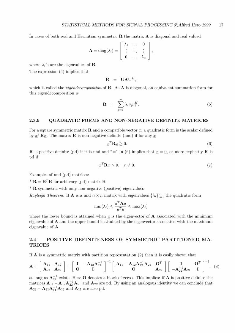
In cases of both real and Hermitian symmetric R the matrix Λ is diagonal and real valued
Λ = diag(λi) =
λ1 . . . 0...
. . ....
0 . . . λn
,
where λi’s are the eigenvalues of R.
The expression (4) implies that
R = UΛUH ,
which is called the eigendecomposition of R. As Λ is diagonal, an equivalent summation form forthis eigendecomposition is
R =n∑
i=1
λiνiνHi . (5)
2.3.9 QUADRATIC FORMS AND NON-NEGATIVE DEFINITE MATRICES
For a square symmetric matrix R and a compatible vector x, a quadratic form is the scalar definedby xTRx. The matrix R is non-negative definite (nnd) if for any x
xTRx ≥ 0. (6)
R is positive definite (pd) if it is nnd and ”=” in (6) implies that x = 0, or more explicitly R ispd if
xTRx > 0, x 6= 0. (7)
Examples of nnd (pd) matrices:
* R = BTB for arbitrary (pd) matrix B
* R symmetric with only non-negative (positive) eigenvalues
Rayleigh Theorem: If A is a nnd n× n matrix with eigenvalues λini=1 the quadratic form
min(λi) ≤ uTAu
uT u≤ max(λi)
where the lower bound is attained when u is the eigenvector of A associated with the minimumeigenvalue of A and the upper bound is attained by the eigenvector associated with the maximumeigenvalue of A.
2.4 POSITIVE DEFINITENESS OF SYMMETRIC PARTITIONED MA-TRICES
If A is a symmetric matrix with partition representation (2) then it is easily shown that
A =[
A11 A12
A21 A22
]=
[I −A12A−1
22
O I
]−1 [A11 −A12A−1
22 A21 OT
O A22
] [I OT
−A−122 A21 I
]−1
, (8)
as long as A−122 exists. Here O denotes a block of zeros. This implies: if A is positive definite the
matrices A11−A12A−122 A21 and A22 are pd. By using an analogous identity we can conclude that
A22 −A21A−111 A12 and A11 are also pd.
STATISTICAL METHODS FOR SIGNAL PROCESSING c©Alfred Hero 1999 18
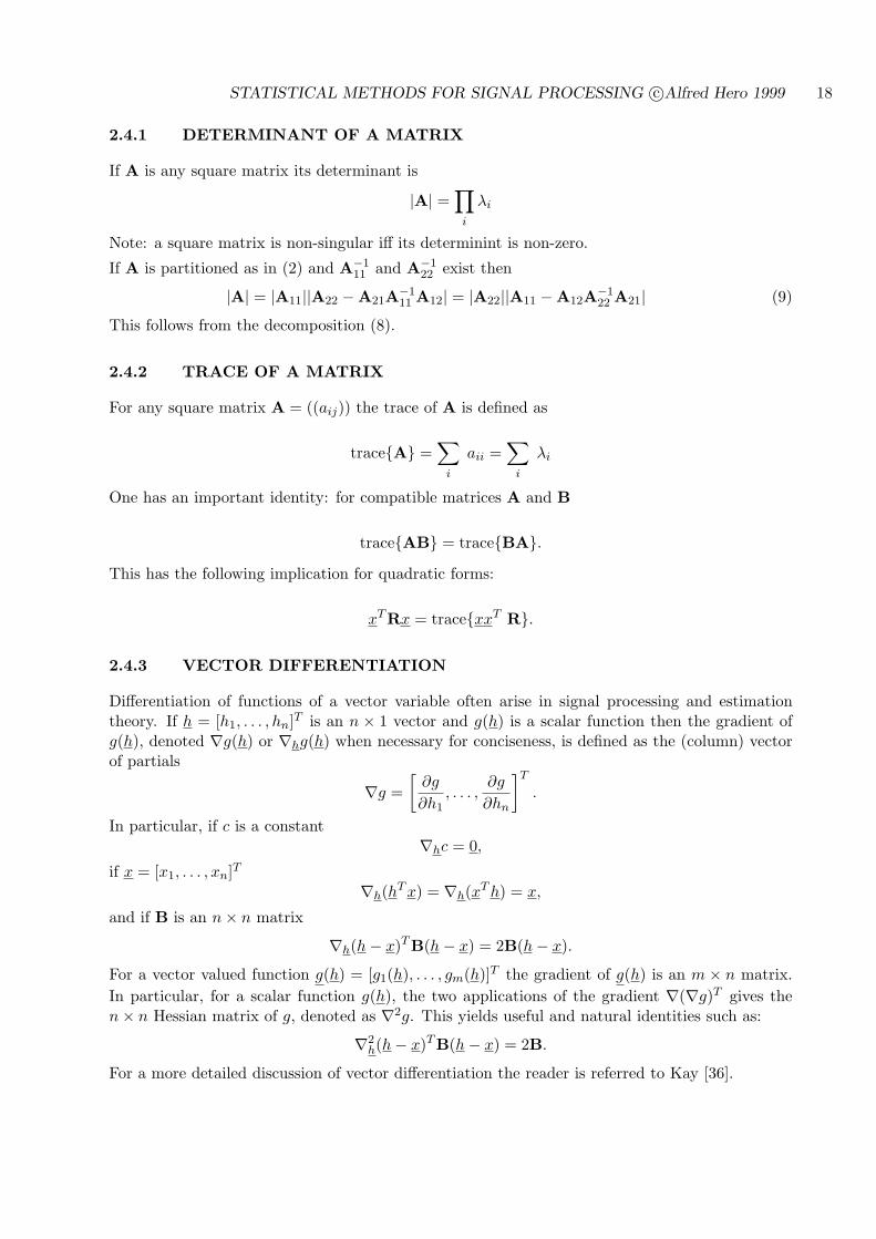
2.4.1 DETERMINANT OF A MATRIX
If A is any square matrix its determinant is
|A| =∏
i
λi
Note: a square matrix is non-singular iff its determinint is non-zero.
If A is partitioned as in (2) and A−111 and A−1
22 exist then
|A| = |A11||A22 −A21A−111 A12| = |A22||A11 −A12A−1
22 A21| (9)
This follows from the decomposition (8).
2.4.2 TRACE OF A MATRIX
For any square matrix A = ((aij)) the trace of A is defined as
traceA =∑
i
aii =∑
i
λi
One has an important identity: for compatible matrices A and B
traceAB = traceBA.This has the following implication for quadratic forms:
xTRx = tracexxT R.
2.4.3 VECTOR DIFFERENTIATION
Differentiation of functions of a vector variable often arise in signal processing and estimationtheory. If h = [h1, . . . , hn]T is an n × 1 vector and g(h) is a scalar function then the gradient ofg(h), denoted ∇g(h) or ∇hg(h) when necessary for conciseness, is defined as the (column) vectorof partials
∇g =[
∂g
∂h1, . . . ,
∂g
∂hn
]T
.
In particular, if c is a constant∇hc = 0,
if x = [x1, . . . , xn]T
∇h(hT x) = ∇h(xT h) = x,
and if B is an n× n matrix
∇h(h− x)TB(h− x) = 2B(h− x).
For a vector valued function g(h) = [g1(h), . . . , gm(h)]T the gradient of g(h) is an m × n matrix.In particular, for a scalar function g(h), the two applications of the gradient ∇(∇g)T gives then× n Hessian matrix of g, denoted as ∇2g. This yields useful and natural identities such as:
∇2h(h− x)TB(h− x) = 2B.
For a more detailed discussion of vector differentiation the reader is referred to Kay [36].
STATISTICAL METHODS FOR SIGNAL PROCESSING c©Alfred Hero 1999 19
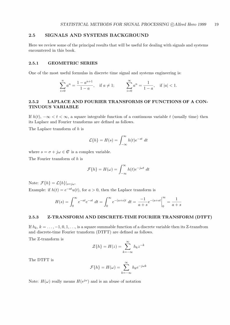
2.5 SIGNALS AND SYSTEMS BACKGROUND
Here we review some of the principal results that will be useful for dealing with signals and systemsencountered in this book.
2.5.1 GEOMETRIC SERIES
One of the most useful formulas in discrete time signal and systems engineering is:
n∑
i=0
an =1− an+1
1− a, if a 6= 1;
∞∑
i=0
an =1
1− a, if |a| < 1.
2.5.2 LAPLACE AND FOURIER TRANSFORMS OF FUNCTIONS OF A CON-TINUOUS VARIABLE
If h(t), −∞ < t < ∞, a square integrable function of a continuous variable t (usually time) thenits Laplace and Fourier transforms are defined as follows.
The Laplace transform of h is
Lh = H(s) =∫ ∞
−∞h(t)e−st dt
where s = σ + jω ∈ Cl is a complex variable.
The Fourier transform of h is
Fh = H(ω) =∫ ∞
−∞h(t)e−jωt dt
Note: Fh = Lh|s=jω.
Example: if h(t) = e−atu(t), for a > 0, then the Laplace transform is
H(s) =∫ ∞
0e−ate−st dt =
∫ ∞
0e−(a+s)t dt =
−1a + s
e−(a+st
∣∣∣∣∞
0
=1
a + s
2.5.3 Z-TRANSFORM AND DISCRETE-TIME FOURIER TRANSFORM (DTFT)
If hk, k = . . . ,−1, 0, 1, . . ., is a square summable function of a discrete variable then its Z-transfromand discrete-time Fourier transform (DTFT) are defined as follows.
The Z-transform is
Zh = H(z) =∞∑
k=−∞hkz
−k
The DTFT is
Fh = H(ω) =∞∑
k=−∞hke
−jωk
Note: H(ω) really means H(ejω) and is an abuse of notation
STATISTICAL METHODS FOR SIGNAL PROCESSING c©Alfred Hero 1999 20
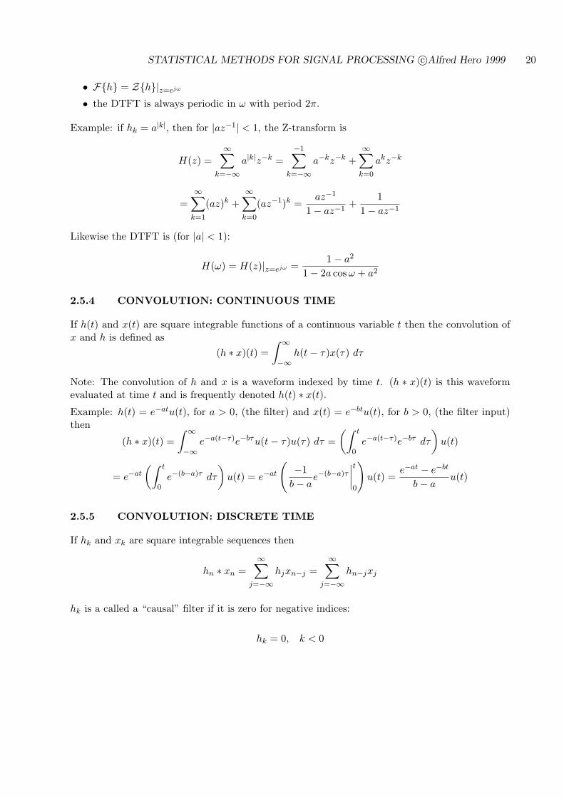
• Fh = Zh|z=ejω
• the DTFT is always periodic in ω with period 2π.
Example: if hk = a|k|, then for |az−1| < 1, the Z-transform is
H(z) =∞∑
k=−∞a|k|z−k =
−1∑
k=−∞a−kz−k +
∞∑
k=0
akz−k
=∞∑
k=1
(az)k +∞∑
k=0
(az−1)k =az−1
1− az−1+
11− az−1
Likewise the DTFT is (for |a| < 1):
H(ω) = H(z)|z=ejω =1− a2
1− 2a cosω + a2
2.5.4 CONVOLUTION: CONTINUOUS TIME
If h(t) and x(t) are square integrable functions of a continuous variable t then the convolution ofx and h is defined as
(h ∗ x)(t) =∫ ∞
−∞h(t− τ)x(τ) dτ
Note: The convolution of h and x is a waveform indexed by time t. (h ∗ x)(t) is this waveformevaluated at time t and is frequently denoted h(t) ∗ x(t).
Example: h(t) = e−atu(t), for a > 0, (the filter) and x(t) = e−btu(t), for b > 0, (the filter input)then
(h ∗ x)(t) =∫ ∞
−∞e−a(t−τ)e−bτu(t− τ)u(τ) dτ =
(∫ t
0e−a(t−τ)e−bτ dτ
)u(t)
= e−at
(∫ t
0e−(b−a)τ dτ
)u(t) = e−at
(−1
b− ae−(b−a)τ
∣∣∣∣t
0
)u(t) =
e−at − e−bt
b− au(t)
2.5.5 CONVOLUTION: DISCRETE TIME
If hk and xk are square integrable sequences then
hn ∗ xn =∞∑
j=−∞hjxn−j =
∞∑
j=−∞hn−jxj
hk is a called a “causal” filter if it is zero for negative indices:
hk = 0, k < 0
STATISTICAL METHODS FOR SIGNAL PROCESSING c©Alfred Hero 1999 21
2.5.6 CORRELATION: DISCRETE TIME
For time sequences xknk=1 and ykn
k=1 their temporal correlation is
zn =n∑
j=1
xky∗k
2.5.7 RELATION BETWEEN CORRELATION AND CONVOLUTION
zn =n∑
j=1
xky∗k =
∞∑
j=−∞xkhn−k = hn ? xn
where
hk =
y∗n−k, k = 1, . . . , n0, o.w.
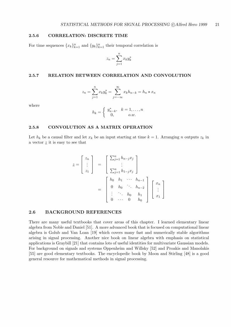
2.5.8 CONVOLUTION AS A MATRIX OPERATION
Let hk be a causal filter and let xk be an input starting at time k = 1. Arranging n outputs zk ina vector z it is easy to see that
z =
zn...z1
=
∑nj=1 hn−jxj
...∑nj=1 h1−jxj
=
h0 h1 · · · hn−1
0 h0. . . hn−2
.... . . h0 h1
0 · · · 0 h0
xn...
x1
2.6 BACKGROUND REFERENCES
There are many useful textbooks that cover areas of this chapter. I learned elementary linearalgebra from Noble and Daniel [51]. A more advanced book that is focused on computational linearalgebra is Golub and Van Loan [19] which covers many fast and numerically stable algorithmsarising in signal processing. Another nice book on linear algebra with emphasis on statisticalapplications is Graybill [21] that contains lots of useful identities for multivariate Gaussian models.For background on signals and systems Oppenheim and Willsky [52] and Proakis and Manolakis[55] are good elementary textbooks. The encyclopedic book by Moon and Stirling [48] is a goodgeneral resource for mathematical methods in signal processing.
STATISTICAL METHODS FOR SIGNAL PROCESSING c©Alfred Hero 1999 22
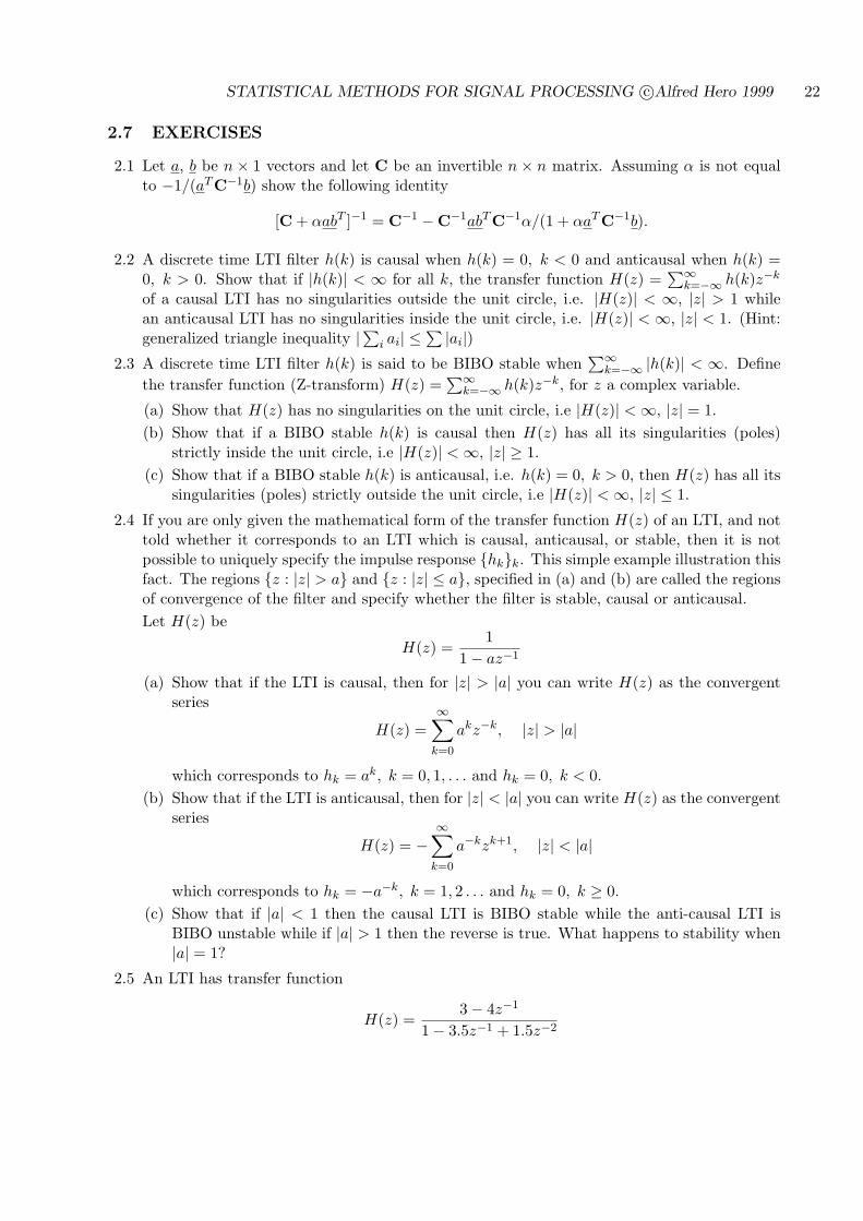
2.7 EXERCISES
2.1 Let a, b be n × 1 vectors and let C be an invertible n × n matrix. Assuming α is not equalto −1/(aTC−1b) show the following identity
[C + αabT ]−1 = C−1 −C−1abTC−1α/(1 + αaTC−1b).
2.2 A discrete time LTI filter h(k) is causal when h(k) = 0, k < 0 and anticausal when h(k) =0, k > 0. Show that if |h(k)| < ∞ for all k, the transfer function H(z) =
∑∞k=−∞ h(k)z−k
of a causal LTI has no singularities outside the unit circle, i.e. |H(z)| < ∞, |z| > 1 whilean anticausal LTI has no singularities inside the unit circle, i.e. |H(z)| < ∞, |z| < 1. (Hint:generalized triangle inequality |∑i ai| ≤
∑ |ai|)2.3 A discrete time LTI filter h(k) is said to be BIBO stable when
∑∞k=−∞ |h(k)| < ∞. Define
the transfer function (Z-transform) H(z) =∑∞
k=−∞ h(k)z−k, for z a complex variable.
(a) Show that H(z) has no singularities on the unit circle, i.e |H(z)| < ∞, |z| = 1.(b) Show that if a BIBO stable h(k) is causal then H(z) has all its singularities (poles)
strictly inside the unit circle, i.e |H(z)| < ∞, |z| ≥ 1.(c) Show that if a BIBO stable h(k) is anticausal, i.e. h(k) = 0, k > 0, then H(z) has all its
singularities (poles) strictly outside the unit circle, i.e |H(z)| < ∞, |z| ≤ 1.
2.4 If you are only given the mathematical form of the transfer function H(z) of an LTI, and nottold whether it corresponds to an LTI which is causal, anticausal, or stable, then it is notpossible to uniquely specify the impulse response hkk. This simple example illustration thisfact. The regions z : |z| > a and z : |z| ≤ a, specified in (a) and (b) are called the regionsof convergence of the filter and specify whether the filter is stable, causal or anticausal.Let H(z) be
H(z) =1
1− az−1
(a) Show that if the LTI is causal, then for |z| > |a| you can write H(z) as the convergentseries
H(z) =∞∑
k=0
akz−k, |z| > |a|
which corresponds to hk = ak, k = 0, 1, . . . and hk = 0, k < 0.(b) Show that if the LTI is anticausal, then for |z| < |a| you can write H(z) as the convergent
series
H(z) = −∞∑
k=0
a−kzk+1, |z| < |a|
which corresponds to hk = −a−k, k = 1, 2 . . . and hk = 0, k ≥ 0.(c) Show that if |a| < 1 then the causal LTI is BIBO stable while the anti-causal LTI is
BIBO unstable while if |a| > 1 then the reverse is true. What happens to stability when|a| = 1?
2.5 An LTI has transfer function
H(z) =3− 4z−1
1− 3.5z−1 + 1.5z−2

STATISTICAL METHODS FOR SIGNAL PROCESSING c©Alfred Hero 1999 23
(a) If you are told that the LTI is stable specify the region of convergence (ROC) in thez-plane, i.e. specify the range of values of |z| for which |H(z)| < ∞, and specify theimpulse response.
(b) If you are told that the LTI is causal specify the region of convergence (ROC) in thez-plane, and specify the impulse response.
(c) If you are told that the LTI is anticausal specify the region of convergence (ROC) in thez-plane, and specify the impulse response.
End of chapter
STATISTICAL METHODS FOR SIGNAL PROCESSING c©Alfred Hero 1999 24
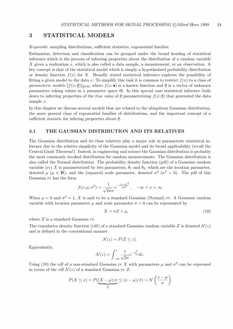
3 STATISTICAL MODELS
Keywords: sampling distributions, sufficient statistics, exponential families.
Estimation, detection and classification can be grouped under the broad heading of statisticalinference which is the process of inferring properties about the distribution of a random variableX given a realization x, which is also called a data sample, a measurement, or an observation. Akey concept is that of the statistical model which is simply a hypothesized probability distributionor density function f(x) for X. Broadly stated statistical inference explores the possibility offitting a given model to the data x. To simplify this task it is common to restrict f(x) to a class ofparameteric models f(x; θ)θ∈Θ, where f(x; •) is a known function and θ is a vector of unknownparameters taking values in a parameter space Θ. In this special case statistical inference boilsdown to inferring properties of the true value of θ parameterizing f(x; θ) that generated the datasample x.
In this chapter we discuss several models that are related to the ubiquitous Gaussian distribution,the more general class of exponential families of distributions, and the important concept of asufficient statistic for infering properties about θ.
3.1 THE GAUSSIAN DISTRIBUTION AND ITS RELATIVES
The Gaussian distribution and its close relatives play a major role in parameteric statistical in-ference due to the relative simplicity of the Gaussian model and its broad applicability (recall theCentral Limit Theorem!). Indeed, in engineering and science the Gaussian distribution is probablythe most commonly invoked distribution for random measurements. The Gaussian distribution isalso called the Normal distribution. The probability density function (pdf) of a Gaussian randomvariable (rv) X is parameterized by two parameters, θ1 and θ2, which are the location parameter,denoted µ (µ ∈ IR), and the (squared) scale parameter, denoted σ2 (σ2 > 0). The pdf of thisGaussian rv has the form
f(x;µ, σ2) =1√2πσ
e−(x−µ)2
2σ2 , −∞ < x < ∞
When µ = 0 and σ2 = 1, X is said to be a standard Gaussian (Normal) rv. A Gaussian randomvariable with location parameter µ and scale parameter σ > 0 can be represented by
X = σZ + µ, (10)
where Z is a standard Gaussian rv.
The cumulative density function (cdf) of a standard Gaussian random variable Z is denoted N (z)and is defined in the conventional manner
N (z) = P (Z ≤ z).
Equivalently,
N (z) =∫ z
−∞
1√2π
e−v2
2 dv.
Using (10) the cdf of a non-standard Gaussian rv X with parameters µ and σ2 can be expressedin terms of the cdf N (z) of a standard Gaussian rv Z:
P (X ≤ x) = P ((X − µ)/σ︸ ︷︷ ︸Z
≤ (x− µ)/σ) = N(
x− µ
σ
)

STATISTICAL METHODS FOR SIGNAL PROCESSING c©Alfred Hero 1999 25
The standard Normal cdf N (x) can be related to the error function or error integral [1]: erf(u) =2√π
∫ u0 e−t2dt, x ≥ 0, through the relation
N (x) =
12 [1 + erf(|x|/√2)] x ≥ 012 [1− erf(|x|/√2)], x < 0
.
For positive integer order ν, the moments of a standard Gaussian random variable Z are [30, 13.3]
E[Zν ] =
(ν − 1)(ν − 3) · · · 3 · 1, ν even0, ν odd
where E[g(Z)] =∫∞−∞ g(z)f(z)dz denotes statistical expectation of the rv g(Z) under the pdf
f(z) for rv Z. These moment relations can easily be derived by looking at the coefficients of(ju)k/k!, k = 1, 2, . . . in the power series expansion about ju = 0 of the characteristic functionΦZ(u) = E[ejuZ ] = e−u2/2.
In particular, using (10), this implies that the first and second moments of a non-standard Gaussianrv X are E[X] = µ and E[X2] = µ2 + σ2, respectively. Thus for a Gaussian rv X we can identifythe (ensemble) mean E[X] = µ and variance var(X) = E[(X − E[X])2] = E[X2] − E2[X] = σ2
as the location and (squared) scale parameters, respectively, of the pdf f(x; µ, σ2) of X. In thesequel we will need the following expression for the (non-central) mean deviation E[|X + a|] forGaussian X [31, 29.6]:
E[|X + a|] =
√2π
e−a2/2 + a(1− 2N (−a)). (11)
In referring to rv’s and operations on rv’s in this book the following compact notations are some-times used:
* “X is distributed as a Gaussian random variable with mean µ and variance σ2”
X ∼ N (µ, σ2) (12)
* “X is equal to a scaled and shifted standard Gaussian random variable”
X = a Z︸︷︷︸N (0,1)
+b ⇔ X ∼ N (b, a2)
or, in shorthand notation,
X = a N (0, 1) + b ⇔ X ∼ N (b, a2). (13)
For example, in the following shorthand notation X1, . . . , Xn are independent identically distrib-uted (iid) N (0, 1) rv’s
n∑
i=1
N (0, 1) =n∑
i=1
Xi.
Note that the above is an abuse of notation since N (0, 1) is being used to denote both a Gaussianprobability distribution in (12) and a Gaussian random variable in (13). As in all abuses of this
STATISTICAL METHODS FOR SIGNAL PROCESSING c©Alfred Hero 1999 26
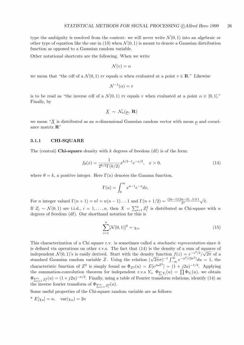
type the ambiguity is resolved from the context: we will never write N (0, 1) into an algebraic orother type of equation like the one in (13) when N (0, 1) is meant to denote a Gaussian distributionfunction as opposed to a Gaussian random variable.
Other notational shortcuts are the following. When we write
N (v) = α
we mean that “the cdf of a N (0, 1) rv equals α when evaluated at a point v ∈ IR.” Likewise
N−1(α) = v
is to be read as “the inverse cdf of a N (0, 1) rv equals v when evaluated at a point α ∈ [0, 1].”Finally, by
X ∼ Nn(µ, R)
we mean “X is distributed as an n-dimensional Gaussian random vector with mean µ and covari-ance matrix R”
3.1.1 CHI-SQUARE
The (central) Chi-square density with k degrees of freedom (df) is of the form:
fθ(x) =1
2k/2Γ(k/2)xk/2−1e−x/2, x > 0, (14)
where θ = k, a positive integer. Here Γ(u) denotes the Gamma function,
Γ(u) =∫ ∞
0xu−1e−xdx,
For n integer valued Γ(n + 1) = n! = n(n− 1) . . . 1 and Γ(n + 1/2) = (2n−1)(2n−3)...5·3·12n
√π.
If Zi ∼ N (0, 1) are i.i.d., i = 1, . . . , n, then X =∑n
i=1 Z2i is distributed as Chi-square with n
degrees of freedom (df). Our shorthand notation for this is
n∑
i=1
[N (0, 1)]2 = χn. (15)
This characterization of a Chi square r.v. is sometimes called a stochastic representation since itis defined via operations on other r.v.s. The fact that (14) is the density of a sum of squares ofindependent N (0, 1)’s is easily derived. Start with the density function f(z) = e−z2/2/
√2π of a
standard Gaussian random variable Z. Using the relation (√
2πσ)−1∫∞−∞ e−u2/(2σ2)du = 1, the
characteristic function of Z2 is simply found as ΦZ2(u) = E[ejuZ2] = (1 + j2u)−1/2. Applying
the summation-convolution theorem for independent r.v.s Yi, ΦPYi(u) =
∏ΦYi(u), we obtain
ΦPni=1 Z2
i(u) = (1 + j2u)−n/2. Finally, using a table of Fourier transform relations, identify (14) as
the inverse fourier transform of ΦPni=1 Z2
i(u).
Some useful properties of the Chi-square random variable are as follows:
* E[χn] = n, var(χn) = 2n
STATISTICAL METHODS FOR SIGNAL PROCESSING c©Alfred Hero 1999 27
* Asymptotic relation for large n:
χn =√
2nN (0, 1) + n
* χ2 an exponential r.v. with mean 2, i.e. X = χ2 is a non-negative r.v. with probability densityf(x) = 1
2e−x/2.
*√
χ2 is a Rayleigh distributed random variable.
3.1.2 GAMMA
The Gamma density function is
fθ(x) =λr
Γ(r)xr−1e−λx, x > 0,
where θ denotes the pair of parameters (λ, r), λ, r > 0. Let Yini=1 be i.i.d. exponentially
distributed random variables with mean 1/λ, specifically Yi has density
fλ(y) = λe−λy, y > 0.
Then the sum X =∑n
i=1 Yi has a Gamma density f(λ,n). Other useful properties of a Gammadistributed random variable X with parameters θ = (λ, r) include:
* Eθ[X] = r/λ
* varθ(X) = r/λ2
* The Chi-square distribution with k df is a special case of the Gamma distribution obtained bysetting Gamma parameters as follows: λ = 1/2 and r = k/2.
3.1.3 NON-CENTRAL CHI SQUARE
The sum of squares of independent Gaussian r.v.s with unit variances but non-zero means is calleda non-central Chi-square r.v. Specifically, if Zi ∼ N (µi, 1) are independent, i = 1, . . . , n, thenX =
∑ni=1 Z2
i is distributed as non-central Chi-square with n df and non-centrality parameterδ =
∑ni=1 µ2
i . In our shorthand we write
n∑
i=1
[N (0, 1) + µi]2 =n∑
i=1
[N (µi, 1)]2 = χn,δ. (16)
The non-central Chi-square density has no simple expression of closed form. There are some usefulasymptotic relations, however:
* E[χn,δ] = n + δ, var(χn,δ) = 2(n + 2δ)
* √χ2,µ2
1+µ22
is a Rician r.v.
STATISTICAL METHODS FOR SIGNAL PROCESSING c©Alfred Hero 1999 28
3.1.4 CHI-SQUARE MIXTURE
The distribution of the sum of squares of independent Gaussian r.v.s with zero mean but differentvariances is not closed form either. However, many statisticians have studied and tabulated thedistribution of a weighted sum of squares of i.i.d. standard Gaussian r.v.s Z1, . . . , Zn, Zi ∼ N (0, 1).Specifically, the following has a (central) Chi-square mixture (also known as the Chi-bar square[30]) with n degrees of freedom and mixture parameter c = [c1, . . . , cn]T , ci ≥ 0:
n∑
i=1
ci∑j cj
Z2i = χn,c
An asymptotic relation of interest to us will be:
* E[χn,c] = 1, , var(χn,c) = 2∑N
i=1
(ciPj ci
)2
Furthermore, there is an obvious a special case where the Chi square mixture reduces to a scaled(central) Chi square: χn,c1 = 1
n χn for any c 6= 0.
3.1.5 STUDENT-T
For Z ∼ N (0, 1) and Y ∼ χn independent r.v.s the ratio X = Z/√
Y/n is called a Student-t r.v.with n degrees of freedom, denoted Tn. Or in our shorthand notation:
N (0, 1)√χn/n
= Tn.
The density of Tn is the Student-t density with n df and has the form
fθ(x) =Γ([n + 1]/2)
Γ(n/2)1
n√
π
1(1 + x2)(n+1)/2
, x ∈ IR,
where θ = n is a positive integer. Properties of interest to us are:
* E[Tn] = 0 (n > 1), var(Tn) = nn−2 (n > 2)
* Asymptotic relation for large n:
Tn ≈ N (0, 1).
For n = 1 the mean of Tn does not exist and for n ≤ 2 its variance is infinite.
3.1.6 FISHER-F
For U ∼ χm and V ∼ χn independent r.v.s the ratio X = (U/m)/(V/n) is called a Fisher-F r.v.with m, n degrees of freedom, or in shorthand:
χm/m
χn/n= Fm,n.
The Fisher-F density with m and n df is defined as
fθ(x) =Γ([m + n]/2)Γ(m/2)Γ(n/2)
(m
n
)m/2 x(m−2)/2
(1 + mn x)(m+n)/2
, x > 0
STATISTICAL METHODS FOR SIGNAL PROCESSING c©Alfred Hero 1999 29
where θ = [m, n] is a pair of positive integers. It should be noted that moments E[Xk] of ordergreater than k = n/2 do not exist. A useful asymptotic relation for n large and n À m is
Fm,n ≈ χm.
3.1.7 CAUCHY
The ratio of independent N (0, 1) r.v.’s U and V is called a standard Cauchy r.v.
X = U/V ∼ C(0, 1).
It’s density has the form
f(x) =1π
11 + x2
x ∈ IR
. If θ = [µ, σ] are location and scale parameters (σ > 0) fθ(x) = f((x − µ)/σ) is a translatedand scaled version of the standard Cauchy density denoted C(µ, σ2). Some properties of note:(1) the Cauchy distribution has no moments of any (positive) integer order; and (2) the Cauchydistribution is the same as a Student-t distribution with 1 d.f.
3.1.8 BETA
For U ∼ χm and V ∼ χn independent Chi-square r.v.s with m and n df, respectively, the ratioX = U/(U + V ) has a Beta distribution, or in shorthand
χm
χm + χn= B(m/2, n/2)
where B(p, q) is a r.v. with Beta density having paramaters θ = [p, q]. The Beta density has theform
fθ(x) =1
βr,txr−1(1− x)t−1, x ∈ [0, 1]
where θ = [r, t] and r, t > 0. Here βr,t is the Beta function:
βr,t =∫ 1
0xr−1(1− x)t−1dx =
Γ(r)Γ(t)Γ(r + t)
.
Some useful properties:
* The special case of m = n = 1 gives rise to X an arcsin distributed r.v.
* Eθ[B(p, q)] = p/(p + q)
* varθ(B(p, q)) = pq/((p + q + 1)(p + q)2)
3.2 REPRODUCING DISTRIBUTIONS
A random variable X is said to have a reproducing distribution if the sum of two independentrealizations, say X1 and X2, of X have the same distribution, possibly with different parametervalues, as X. A Gaussian r.v. has a reproducing distribution:
N (µ1, σ21) +N (µ2, σ
22) = N (µ1 + µ2, σ
21 + σ2
2),
STATISTICAL METHODS FOR SIGNAL PROCESSING c©Alfred Hero 1999 30
which follows from the fact that the convolution of two Gaussian density functions is a Gaussiandensity function [47]. Noting the stochastic representations (15) and (16) of the Chi square andnon-central Chi square distributions, respectively, it is obvious that they are reproducing distrib-utions:
*χn + χm = χm+n, if χm, χn are independent.
*χm,δ1 + χn,δ2 = χm+n,δ1+δ2 , if χm,δ1 , χn,δ2 are independent.
The Chi square mixture, Fisher-F, and Student-t are not reproducing densities.
3.3 FISHER-COCHRAN THEOREM
This result gives a very useful tool for finding the distribution of quadratic forms of Gaussianrandom variables. A more general result that covers the joint distribution of quadratic forms isgiven in [56].
Theorem 1 Let X = [X1, . . . , Xn]T be a vector of iid. N (0, 1) rv’s and let A be a symmetricidempotent matrix (AA = A) of rank p. Then
XTAX = χp
A simple proof is given below.
Proof: Let A = UΛUT be the eigendecomposition of A. Then
* All eigenvalues λi of A are either 0 or 1
AA = UΛUTU︸ ︷︷ ︸=I
ΛUT
= UΛ2UT = UΛUT
and therefore
XTAX = XTUΛ UT X︸ ︷︷ ︸Z=Nn(0,I)
=n∑
i=1
λiZ2i =
p∑
i=1
[N (0, 1)]2
¦
3.4 SAMPLE MEAN AND SAMPLE VARIANCE
Let Xi’s be i.i.d. N (µ, σ) r.v.’s. The sample mean and sample variance respectively approximatethe location µ and spread σ of the population.
* Sample mean: X = n−1∑n
i=1 Xi
* Sample variance: s2 = 1n−1
∑ni=1(Xi −X)2

STATISTICAL METHODS FOR SIGNAL PROCESSING c©Alfred Hero 1999 31
In the Gaussian case the joint distribution of the sample mean and variance can be specified.
(1). X = N (µ, σ/n)
(2). s2 = σ2
n−1 χn−1
(3). X and s2 are independent rv’s.
These results imply that a weighted ratio of sample mean and sample variance is distributed asStudent t.
X − µ
s/√
n= Tn−1.
Proof of assertions (2) and (3): In view of the representation (13), it suffices consider the the caseof a standard Gaussian sample: µ = 0 and σ = 1.
First we show that the sample mean and the sample variance are independent random variables.Define the vector of random variables Y = [Y1, . . . , Yn]T as follows. First define
Y1 =√
nX = hT1 X,
whereh1 = [1/
√n, . . . , 1/
√n]T .
Note that h1 has unit norm. Next apply the Gramm-Schmidt orthonormalization procedure ofSec. 2.3.6 to complete the basis with respect to h1. This generates n − 1 vectors h2, . . . , hn thatare orthonormal, mutually orthogonal, and orthogonal to h1. The random vector Y is now definedas
Y = HT X
where H = [h1, . . . , hn] is an n× n orthogonal matrix.
Since, X = HY, the orthogonality of H implies the following properties
1. The Yi’s are zero mean unit variance independent Gaussian random variables: Y ∼ Nn(0, I)
2. Y T Y = XT X
As Y 1 =√
nX Property 1 implies that X is independent of Y2, . . . , Yn. Furthermore, using theequivalence:
n∑
i=1
(Xi −X)2 =n∑
i=1
X2i − n(X)2,
Property 2 and the definition of Y1 imply that
n∑
i=1
(Xi −X)2 =n∑
i=1
Y 2i − Y1 = Y2 + · · ·+ Yn, (17)
that is, the sample variance is only a function of Y2, . . . , Yn and is therefore independent of Y1 =the sample mean.
Furthermore, as Y2, . . . , Yn are independent N (0, 1) random variables, the representation (17)implies that the (normalized) sample variance has a Chi-square distribution with n− 1 degrees offreedom.
This completes the proof of assertions (2) and (3). ¦
STATISTICAL METHODS FOR SIGNAL PROCESSING c©Alfred Hero 1999 32
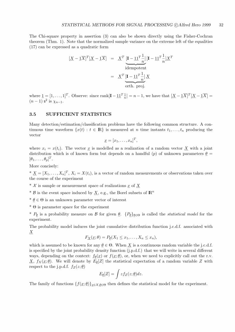
The Chi-square property in assertion (3) can also be shown directly using the Fisher-Cochrantheorem (Thm. 1). Note that the normalized sample variance on the extreme left of the equalities(17) can be expressed as a quadratic form
[X − 1X]T [X − 1X] = XT [I− 11T 1n
]︸ ︷︷ ︸idempotent
[I− 11T 1n
]XT
= XT [I− 11T 1n
]︸ ︷︷ ︸orth. proj.
X
where 1 = [1, . . . , 1]T . Observe: since rank[I− 11T 1n ] = n− 1, we have that [X − 1X]T [X − 1X] =
(n− 1) s2 is χn−1.
3.5 SUFFICIENT STATISTICS
Many detection/estimation/classification problems have the following common structure. A con-tinuous time waveform x(t) : t ∈ IR is measured at n time instants t1, . . . , tn producing thevector
x = [x1, . . . , xn]T ,
where xi = x(ti). The vector x is modelled as a realization of a random vector X with a jointdistribution which is of known form but depends on a handful (p) of unknown parameters θ =[θ1, . . . , θp]T .
More concisely:
* X = [X1, . . . , Xn]T , Xi = X(ti), is a vector of random measurements or observations taken overthe course of the experiment
* X is sample or measurement space of realizations x of X
* B is the event space induced by X, e.g., the Borel subsets of IRn
* θ ∈ Θ is an unknown parameter vector of interest
* Θ is parameter space for the experiment
* Pθ is a probability measure on B for given θ. Pθθ∈Θ is called the statistical model for theexperiment.
The probability model induces the joint cumulative distribution function j.c.d.f. associated withX
FX(x; θ) = Pθ(X1 ≤ x1, . . . , Xn ≤ xn),
which is assumed to be known for any θ ∈ Θ. When X is a continuous random variable the j.c.d.f.is specified by the joint probability density function (j.p.d.f.) that we will write in several differentways, depending on the context: fθ(x) or f(x; θ), or, when we need to explicitly call out the r.v.X, fX(x; θ). We will denote by Eθ[Z] the statistical expectation of a random variable Z withrespect to the j.p.d.f. fZ(z; θ)
Eθ[Z] =∫
zfZ(z; θ)dz.
The family of functions f(x; θ)x∈X ,θ∈Θ then defines the statistical model for the experiment.
STATISTICAL METHODS FOR SIGNAL PROCESSING c©Alfred Hero 1999 33
The general objective of statistical inference can now be stated. Given a realization x of X inferproperties of θ knowing only the parametric form of the statistical model. Thus we will want tocome up with a function, called an inference function, which maps X to subsets of the parameterspace, e.g., an estimator, classifier, or detector for θ. As we will see later there are many ways todesign inference functions but a more fundamental question is: are there any general propertiesthat good inference functions should have? One such property is that the inference function onlyneed depend on the n-dimensional data vector X through a lower dimensional version of the datacalled a sufficient statistic.
3.5.1 SUFFICIENT STATISTICS AND THE REDUCTION RATIO
First we define a statistic as any function T = T (X) of the data (actually, for T to be a validrandom variable derived from X it must be a measurable function, but this theoretical technicalityis beyond our scope here).
There is a nice interpretation of a statistic in terms of its memory storage requirements. Assumethat you have a special computer that can store any one of the time samples in X = [X1, . . . , Xn],Xk = X(tk) say, in a ”byte” of storage space and the time stamp tk in another ”byte” of storagespace. Any non-invertible function T , e.g., which maps IRn to a lower dimensional space IRm,can be viewed as a dimensionality reduction on the data sample. We can quantify the amount ofreduction achieved by T by defining the reduction ratio (RR):
RR =# bytes of storage required for T (X)
# bytes of storage required for X
This ratio is a measure of the amount of data compression induced by a specific transformationT . The number of bytes required to store X with its time stamps is:
# bytesX = # bytes[X1, . . . , Xn]T = # bytestimestamps+ # bytesvalues = 2n
Consider the following examples:
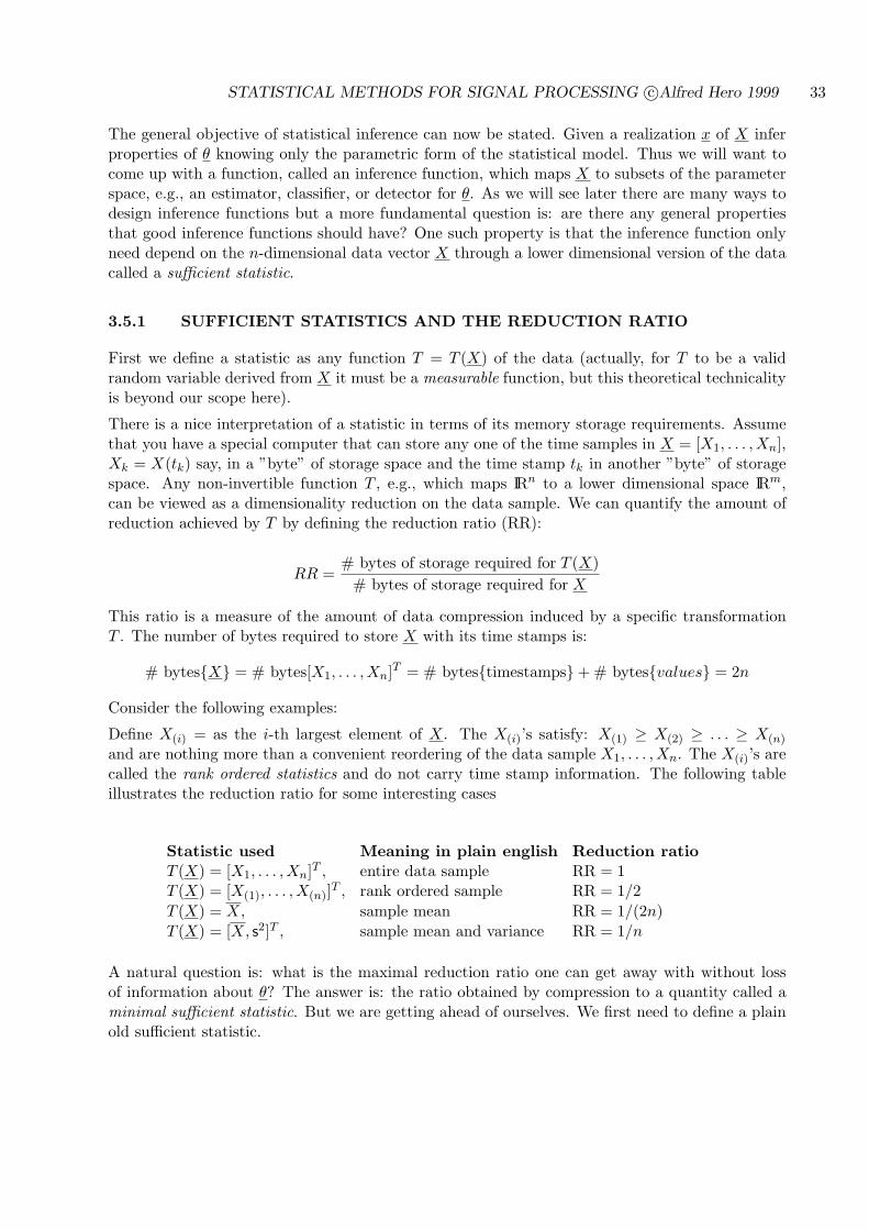
Define X(i) = as the i-th largest element of X. The X(i)’s satisfy: X(1) ≥ X(2) ≥ . . . ≥ X(n)
and are nothing more than a convenient reordering of the data sample X1, . . . , Xn. The X(i)’s arecalled the rank ordered statistics and do not carry time stamp information. The following tableillustrates the reduction ratio for some interesting cases
Statistic used Meaning in plain english Reduction ratioT (X) = [X1, . . . , Xn]T , entire data sample RR = 1T (X) = [X(1), . . . , X(n)]T , rank ordered sample RR = 1/2T (X) = X, sample mean RR = 1/(2n)T (X) = [X, s2]T , sample mean and variance RR = 1/n
A natural question is: what is the maximal reduction ratio one can get away with without lossof information about θ? The answer is: the ratio obtained by compression to a quantity called aminimal sufficient statistic. But we are getting ahead of ourselves. We first need to define a plainold sufficient statistic.
STATISTICAL METHODS FOR SIGNAL PROCESSING c©Alfred Hero 1999 34
3.5.2 DEFINITION OF SUFFICIENCY
Here is a warm up before making a precise definition of sufficiency. T = T (X) is a sufficientstatistic (SS) for a parameter θ if it captures all the information in the data sample useful forinferring the value of θ. To put it another way: once you have computed a sufficient statistic youcan store it and throw away the original sample since keeping it around would not add any usefulinformation.
More concretely, let X have a cumulative distribution function (CDF) FX(x; θ) depending on θ.A statistic T = T (X) is said to be sufficient for θ if the conditional CDF of X given T = t is nota function of θ, i.e.,
FX|T (x|T = t, θ) = G(x, t), (18)
where G is a function that does not depend on θ.
Specializing to a discrete valued X with probability mass function pθ(x) = Pθ(X = x), a statisticT = T (X) is sufficient for θ if
Pθ(X = x|T = t) = G(x, t). (19)
For a continuous r.v. X with pdf f(x; θ), the condition (18) for T to be a sufficient statistic (SS)becomes:
fX|T (x|t; θ) = G(x, t). (20)
Sometimes the only sufficient statistics are vector statistics, e.g. T (X) = T (X) = [T1(X), . . . , TK(X)]T .In this case we say that the Tk’s are jointly sufficient for θ
The definition (18) is often difficult to use since it involves derivation of the conditional distributionof X given T . When the random variable X is discrete or continuous a simpler way to verifysufficiency is through the Fisher factorization (FF) property [56]
Fisher factorization (FF): T = T (X) is a sufficient statistic for θ if the probability densityfX(x; θ) of X has the representation
fX(x; θ) = g(T, θ) h(x), (21)
for some non-negative functions g and h. The FF can be taken as the operational definition ofa sufficient statistic T . An important implication of the Fisher Factorization is that when thedensity function of a sample X satisfies (21) then the density fT (t; θ) of the sufficient statistic Tis equal to g(t, θ) up to a θ-independent constant q(t) (see exercises at end of this chapter):
fT (t; θ) = g(t, θ)q(t).
Examples of sufficient statistics:
Example 1 Entire sample
X = [X1, . . . , Xn]T is sufficient but not very interesting
Example 2 Rank ordered sample
STATISTICAL METHODS FOR SIGNAL PROCESSING c©Alfred Hero 1999 35
X(1), . . . , X(n) is sufficient when Xi’s i.i.d.
Proof: Since Xi’s are i.i.d., the joint pdf is
fθ(x1, . . . , xn) =n∏
i=1
fθ(xi) =n∏
i=1
fθ(x(i)).
Hence sufficiency of the rank ordered sample X(1), . . . , X(n) follows from Fisher factorization.
Example 3 Binary likelihood ratios
Let θ take on only two possible values θ0 and θ1. Then, as f(x; θ) can only be f(x; θ0) or f(x; θ1),we can reindex the pdf as f(x; θ) with the scalar parameter θ ∈ Θ = 0, 1. This gives the binarydecision problem: “decide between θ = 0 versus θ = 1.” If it exists, i.e. it is finite for all values
of X, the “likelihood ratio” Λ(X) = f1(X)/f0(X) is sufficient for θ, where f1(x) def= f(x; 1) and
f0(x) def= f(x; 0).
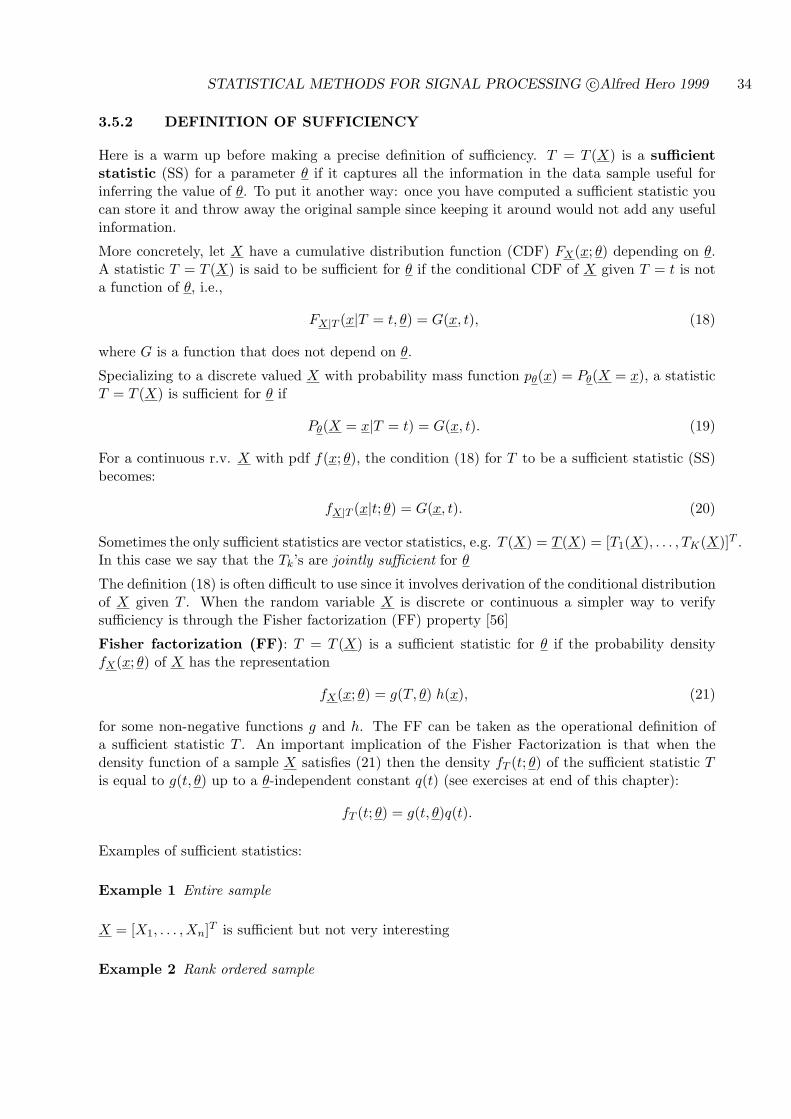
Proof: Express fθ(X) as function of θ, f0, f1, factor out f0, identify Λ, and invoke FF
fθ(X) = θf1(X) + (1− θ)f0(X)
=
θΛ(X) + (1− θ)︸ ︷︷ ︸
g(T,θ)
f0(X)︸ ︷︷ ︸
h(X)
.
¦Therefore to discriminate between two values θ1 and θ2 of a parameter vector θ we can throw awayall data except for the scalar sufficient statistic T = Λ(X)
Example 4 Discrete likelihood ratios
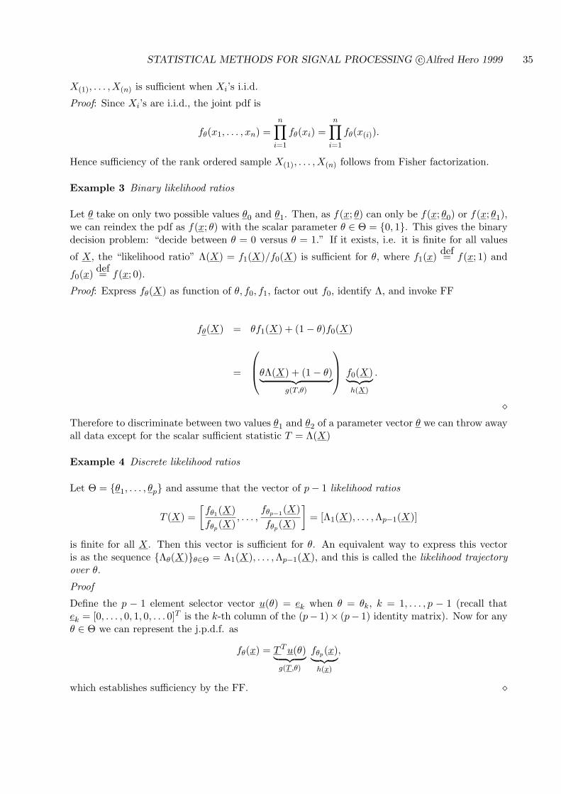
Let Θ = θ1, . . . , θp and assume that the vector of p− 1 likelihood ratios
T (X) =[fθ1(X)fθp(X)
, . . . ,fθp−1(X)fθp(X)
]= [Λ1(X), . . . , Λp−1(X)]
is finite for all X. Then this vector is sufficient for θ. An equivalent way to express this vectoris as the sequence Λθ(X)θ∈Θ = Λ1(X), . . . ,Λp−1(X), and this is called the likelihood trajectoryover θ.
Proof
Define the p − 1 element selector vector u(θ) = ek when θ = θk, k = 1, . . . , p − 1 (recall thatek = [0, . . . , 0, 1, 0, . . . 0]T is the k-th column of the (p− 1)× (p− 1) identity matrix). Now for anyθ ∈ Θ we can represent the j.p.d.f. as
fθ(x) = T T u(θ)︸ ︷︷ ︸g(T ,θ)
fθp(x)︸ ︷︷ ︸h(x)
,
which establishes sufficiency by the FF. ¦

STATISTICAL METHODS FOR SIGNAL PROCESSING c©Alfred Hero 1999 36
Example 5 Likelihood ratio trajectory
When Θ is a set of scalar parameters θ the likelihood ratio trajectory over Θ
Λ(X) =
fθ(X)fθ0(X)
θ∈Θ
, (22)
is sufficient for θ. Here θ0 is an arbitrary reference point in Θ for which the trajectory is finite forall X. When θ is not a scalar (22) becomes a likelihood ratio surface, which is also a sufficientstatistic.
3.5.3 MINIMAL SUFFICIENCY
What is the maximum possible amount of reduction one can apply to the data sample withoutlosing information concerning how the model depends on θ? The answer to this question lies in thenotion of a minimal sufficient statistic. Such statistics cannot be reduced any further without lossin information. In other words, any other sufficient statistic can be reduced down to a minimalsufficient statistic without information loss. Since reduction of a statistic is accomplished byapplying a functional transformation we have the formal definition.
Definition: Tmin is a minimal sufficient statistic if it can be obtained from any other sufficientstatistic T by applying a functional transformation to T . Equivalently, if T is any sufficient statisticthere exists a function q such that Tmin = q(T ).
Note that minimal sufficient statistics are not unique: if Tmin is minimal sufficient h(Tmin) is alsominimally sufficient for h any invertible function. Minimal sufficient statistics can be found in avariety of ways [47, 7, 40]. One way is to find a complete sufficient statistic; under broad conditionsthis statistic will also be minimal [40]. A sufficient statistic T is complete if
Eθ[g(T )] = 0, for all θ ∈ Θ
implies that the function g is identically zero, i.e., g(t) = 0 for all values of t. However, in somecases there are minimal sufficient statistics that are not complete so this is not a failsafe procedure.Another way to find a minimal sufficient statistic is through reduction of the data to the likelihoodratio surface.
As in Example 5, assume that there exists a reference point θo ∈ Θ such that the followinglikelihood-ratio function is finite for all x ∈ X and all θ ∈ Θ
Λθ(x) =fθ(x)fθo
(x).
For given x let Λ(x) denote the set of likelihood ratios (a likelihood ratio trajectory or surface)
Λ(x) = Λθ(x)θ∈Θ.
Definition 1 We say that a (θ-independent) function of x, denoted τ = τ(x), indexes the likeli-hood ratios Λ when both
1. Λ(x) = Λ(τ), i.e., Λ only depends on x through τ = τ(x).
2. Λ(τ) = Λ(τ ′) implies τ = τ ′, i.e., the mapping τ → Λ(τ) is invertible.

STATISTICAL METHODS FOR SIGNAL PROCESSING c©Alfred Hero 1999 37
Condition 1 is an equivalent way of stating that τ(X) is a sufficient statistic for θ.
Theorem:If τ = τ(x) indexes the likelihood ratios Λ(x) then Tmin = τ(X) is minimally sufficientfor θ.
Proof:
We prove this only for the case that X is a continuous r.v. First, condition 1 in Definition 1 impliesthat τ = τ(X) is a sufficient statistic. To see this use FF and the definition of the likelihood ratiosto see that Λ(x) = Λ(τ) implies: fθ(X) = Λθ(τ)fθo
(X) = g(τ ; θ)h(x). Second, let T be anysufficient statistic. Then, again by FF, fθ(x) = g(T, θ) h(x) and thus
Λ(τ) =
fθ(X)fθo
(X)
θ∈Θ
=
g(T, θ)g(T, θo)
θ∈Θ
.
so we conclude that Λ(τ) is a function of T . But by condition 2 in Definition 1 the mappingτ → Λ(τ) is invertible and thus τ is itself a function of T . ¦Another important concept in practical applications is that of finite dimensionality of a sufficientstatistic.
Definition: a sufficient statistic T (X) is said to be finite dimensional if its dimension is not afunction of the number of data samples n.
Frequently, but not always (see Cauchy example below), minimal sufficient statistics are finitedimensional.
Example 6 Minimal sufficient statistic for mean of Gaussian density.
Assume X ∼ N (µ, σ2) where σ2 is known. Find a minimal sufficient statistic for θ = µ given theiid sample X = [X1, . . . , Xn]T .
Solution: the j.p.d.f. is
fθ(x) =(
1√2πσ2
)n
e−1
2σ2
Pni=1(xi−µ)2
=(
1√2πσ2
)n
e−1
2σ2 (Pn
i=1 x2i−2µ
Pni=1 xi+nµ2)
= e−nµ2
2σ2 e
µ/σ2
T (x)︷ ︸︸ ︷n∑
i=1
xi
︸ ︷︷ ︸g(T ,θ)
(1√
2πσ2
)n
e−1/(2σ2)Pn
i=1 x2i
︸ ︷︷ ︸h(x)
Thus by FF
T =n∑
i=1
Xi
is a sufficient statistic for µ. Furthermore, as q(T ) = n−1T is a 1-1 function of T
S = X
STATISTICAL METHODS FOR SIGNAL PROCESSING c©Alfred Hero 1999 38
is an equivalent sufficient statistic.
Next we show that the sample mean is in fact minimal sufficient by showing that it indexes thelikelihood ratio trajectory Λ(x) = Λθ(x)θ∈Θ, with θ = µ, Θ = IR. Select the reference pointθo = µo = 0 to obtain:
Λµ(x) =fµ(x)f0(x)
= exp
(µ/σ2
n∑
i=1
xi − 12nµ2/σ2
).
Identifying τ =∑n
i=1 xi, condition 1 in Definition 1 is obviously satisfied since Λµ(x) = Λµ(∑
xi)(we already knew this since we showed that
∑ni=1 Xi was a sufficient statistic). Condition 2 in
Definition 1 follows since Λµ(∑
xi) is an invertible function of∑
xi for any non-zero value of µ(summation limits omitted for clarity). Therefore the sample mean indexes the trajectories, andis minimal sufficient.
Example 7 Minimal sufficient statistics for mean and variance of Gaussian density.
Assume X ∼ N (µ, σ2) where both µ and σ2 are unknown. Find a minimal sufficient statistic forθ = [µ, σ2]T given the iid sample X = [X1, . . . , Xn]T .
Solution:
fθ(x) =(
1√2πσ2
)n
e−1
2σ2
Pni=1(xi−µ)2
=(
1√2πσ2
)n
e−1
2σ2 (Pn
i=1 x2i−2µ
Pni=1 xi+nµ2)
=(
1√2πσ2
)n
e−nµ2
2σ2 e
[µ/σ2, −1/(2σ2)]
T (x)︷ ︸︸ ︷[n∑
i=1
xi,n∑
i=1
x2i
]T
︸ ︷︷ ︸g(T ,θ)
1︸︷︷︸h(x)
Thus
T =
n∑
i=1
Xi
︸ ︷︷ ︸T1
,n∑
i=1
X2i
︸ ︷︷ ︸T2
is a (jointly) sufficient statistic for µ, σ2. Furthermore, as q(T ) = [n−1T1, (n− 1)−1(T2 − T 21 )] is a
1-1 function of T (T = [T1, T2]T )S =
[X, s2
]
is an equivalent sufficient statistic.
Similarly to Example 6, we can show minimal sufficiency of this statistic by showing that it indexesthe likelihood ratio surface Λθ(X)θ∈Θ, with θ = [µ, σ2], Θ = IR × IR+. Arbitrarily select thereference point θo = [µo, σ
2o ] = [0, 1] to obtain:
Λθ(x) =fθ(x)fθo(x)
=(σo
σ
)ne−nµ2/(2σ2) e[µ/σ2, −δ/2][
Pni=1 xi,
Pni=1 x2
i ]T
,
STATISTICAL METHODS FOR SIGNAL PROCESSING c©Alfred Hero 1999 39
where δ = σ2o−σ2
σ2σ2o
. Identifying τ =[∑n
i=1 xi,∑n
i=1 x2i
], again condition 1 in Definition 1 is obviously
satisfied. Condition 2 in Definition 1 requires a bit more work. While Λθ(τ) is no longer aninvertible function of τ for for any single value of θ = [µ, σ2], we can find two values θ ∈ θ1, θ2 inΘ for which the vector function [Λθ1
(τ), Λθ2(τ)] of τ is invertible in τ . Since this vector is specified
by Λ(x), this will imply that τ indexes the likelihood ratios.
To construct this invertible relation denote by λ = [λ1, λ2]T an observed pair of samples [Λθ1(τ), Λθ2
(τ)]T
of the surface Λ(x). Now consider the problem of determining τ from the equation λ = [Λθ1(τ), Λθ2
(τ)]T .Taking the log of both sides and rearranging some terms, we see that this is equivalent to a 2× 2linear system of equations of the form λ′ = Aτ , where A is a matrix involving θo, θ1, θ2 and λ′ is alinear function of lnλ. You can verify that with the selection of θo = [0, 1], θ1 = [1, 1], θ2 = [0, 1/2]we obtain δ = 0 or 1 for θ = θ1 or θ2, respectively, and A = diag(1,−1/2), an invertible matrix.We therefore conclude that the vector [sample mean, sample variance] indexes the trajectories,and this vector is therefore minimal sufficient.
Example 8 Minimal sufficient statistic for the location of a Cauchy distribution
Assume that Xi ∼ f(x; θ) = 1π
11+(x−θ)2
and, as usual, X = [X1, . . . , Xn]T is an i.i.d. sample.Then
f(x; θ) =n∏
i=1
1π
11 + (xi − θ)2
=1πn
1∏ni=1(1 + (xi − θ)2)
.
Here we encounter a difficulty: the denominator is a 2n-degree polynomial in θ whose coefficientscannot be determined without specifying the entire set of all possible cross products xi1 · · ·xip ,p = 1, 2, . . . , n, of the xi’s. Since this requires specifying the entire set of sample values there is nofinite dimensional sufficient statistic. However, each of these cross products is independent of theordering of its factors so the ordered statistic [X(1), . . . , X(n)]T is minimally sufficient.
3.5.4 EXPONENTIAL FAMILY OF DISTRIBUTIONS
Let θ = [θ1, . . . , θp]T take values in some parameter space Θ. The distribution fθ of a r.v. X is amember of the p-parameter exponential family if for all θ ∈ Θ
fθ(x) = a(θ)b(x)e−cT (θ)t(x), −∞ < x < ∞ (23)
for some scalar functions a, b and some p-element vector functions c, t. Note that for any fθ in theexponential family its support set x : fθ(x) > 0 does not depend on θ. Note that, according toour definition, for fθ to be a member of the p-parameter exponential family the dimension of thevectors c(θ) and t(x) must be exactly p. This is to guarantee that the sufficient statistic has thesame dimension as the parameter vector θ. While our definition is the most standard [39, 47, 7],some other books, e.g., [54], allow the dimension of the sufficient statistic to be different from p.However, by allowing this we lose some important properties of exponential families [7].
The parameterization of an exponential family of distributions is not unique. In other words,the exponential family is invariant to changes in parameterization. For example, let fθ, θ > 0,be an the exponential family of densities with θ a positive scalar. If one defines α = 1/θ andgα = f1/θ then gα, α > 0, is also in the exponential family, but possibly with a different definitionof the functions a(·), b(·), c(·) and t(·). More generally, if fθ(x) is a member of the p-dimensionalexponential family then transformation of the parameters by any invertible function of θ preservesmembership in the exponential family.
STATISTICAL METHODS FOR SIGNAL PROCESSING c©Alfred Hero 1999 40
There exists a special parameterization of distributions in the exponential family, called the naturalparameterization, that has important advantages in terms of ease of estimation of these parame-ters. Definition: Let the random variable X have distribution fθ(x) and assume that fθ is inthe exponential family, i.e., it can be expressed in the form (23). fθ is said to have a naturalparameterization if for all θ ∈ Θ: Eθ[t(X)] = θ. In particular, as we will see in the next chapter,this means that having a natural parameterization makes the statistic T = t(X) an unbiased andefficient estimator of θ.
Examples of distributions in the exponential family include: Gaussian with unknown mean orvariance, Poisson with unknown mean, exponential with unknown mean, gamma, Bernoulli withunknown success probability, binomial with unknown success probability, multinomial with un-known cell probabilities. Distributions which are not from the exponential family include: Cauchywith unknown median, uniform with unknown support, Fisher-F with unknown degrees of freedom.
When the statistical model is in the exponential family, sufficient statistics for the model parame-ters have a particularly simple form:
fθ(x) =n∏
i=1
a(θ)b(xi)e−cT (θ)t(xi)
= an(θ) e
−cT (θ)
T︷ ︸︸ ︷n∑
i=1
t(xi)
︸ ︷︷ ︸g(T ,θ)
n∏
i=1
b(xi)
︸ ︷︷ ︸h(x)
Therefore, the following is a p-dimensional sufficient statistic for θ
n∑
i=1
t(Xi) =
[n∑
i=1
t1(Xi), . . . ,n∑
i=1
tp(Xi)
]T
In fact this is a finite dimensional suff. statistic which is complete and minimal [7].
3.5.5 CHECKING IF A DENSITY IS IN THE EXPONENTIAL FAMILY
Due to the many attractive properties of exponential families, in many situations the first questionto be answered is: is the density of my data X a member of this exclusive club? This questionmight arise, for example, if the input to a known filter or other system has a known density andone can compute a mathematical representation of the density of the output of the filter. To checkif the output density is exponential one has to try and manipulate the density into exponentialform, as illustrated in the exercises. If this is difficult the next step is to try and show that thedensity is not in the exponential family. Some properties can be checked immediately, e.g. thatthe parameters space Θ does not depend on the range of X, e.g. as in a uniform density withunknown region of support boundaries. Another simple test is to compute ∂2/∂θ∂x ln fθ(x) andverify that it is not of separable form c′(θ)t′(x) for some functions c and t. This type of questionis explored in the exercises.
STATISTICAL METHODS FOR SIGNAL PROCESSING c©Alfred Hero 1999 41
3.6 BACKGROUND REFERENCES
Mood, Graybill and Boes [47] offers an undergraduate introduction to mathematical statisticswith lots of fun exercises and examples. Two of the classic graduate level text books on linearmultivariate statistics are Rao [56] and Morrison [49]. Manoukian [42] is a reference book giving aconcise compilation of principal results from sampling distribution theory. The book by Johnsonetal [30], is the first of a set of several volumes of a very comprehensive encyclopedia of probabilitydistributions, random variables, and their properties.
3.7 EXERCISES
3.1 Show that the matrix Π = In − 11T /n is symmetric and idempotent, where In is the n × nidentity matrix and 1 = [1, . . . , 1]T is an n-element column vector of 1’s. Show that forx ∈ IRn, Πx is the vector of residuals [x1 − xi, . . . , xn − xi]T where xi is the sample mean ofelements of x. Finally show that if x has the decomposition y + c1 where y has zero (sample)mean and c is an arbitrary scalar, then Πx = y, i.e the matrix Π extracts the zero (sample)mean component of x. It is in this sense that Π is an orthogonal projection matrix onto thespace of zero (sample) mean vectors in IRn.
3.2 Assume that a random vector X = [X1, . . . , Xn]T has a density pθ(x) which depends onan unknown parameter vector θ. In this exercise you will show that if a statistic S =S(X) = [S1(X), . . . , Sk(X)]T satisfies the Fisher Factorization theorem then the conditionaldensity pθ(X|S) is not a function of θ and thus S is a sufficient statistic for θ. In thefollowing you should assume that X is a discrete random vector and that its joint densitypθ(x) = Pθ(X = x) is a probability mass function (i.e. pθ(x) = 0 except for a countablenumber of points x ∈ x1, x2, . . . where pθ(xi) > 0, and
∑xi
pθ(xi) = 1).
(a) Use Bayes rule to establish that
pθ(x|s) def= Pθ(X = x|S = s) =Pθ(S = s|X = x)pθ(x)∑
xi : S(xi)=s pθ(xi),
where the summation of pθ(x) is over all possible realizations xi of the vector X suchthat S(xi) = s.
(b) Show that Pθ(S = s|X = x) is equal to one or zero depending on whether S(x) = s orS(x) 6= s, respectively. (Hint: express the conditional probability as a ratio and use thedefinition S = S(X) to evaluate the intersection of the events S = s and X = x).
(c) Using the Fisher Factorization pθ(x) = gθ(s) · h(x) show that
pθ(x|s) =
h(x)P
xi : S(xi)=s h(xi), S(x) = s
0, o.w.,
which, as claimed, does not depend on θ.
3.3 Show that the Poisson distribution pλ(x) = Pλ(X = x) = λx
x! exp(−λ), x = 0, 1, 2, . . . is amember of the one-parameter exponential family. For an i.i.d. sample X = [X1, . . . , Xn]T ofthese Poisson r.v.s find a one dimensional sufficient statistic for λ. Define α = 1/λ and showthat the reparameterized Poisson distribution pα(x) is also in the exponential family. Whichof these two parameterizations (α or λ) is the natural paramaterization?

STATISTICAL METHODS FOR SIGNAL PROCESSING c©Alfred Hero 1999 42
3.4 Let X = [X1, . . . , Xn]T be a vector of i.i.d. r.v.s Xi which are uniformly distributed over theinterval (θ1, θ2), θ1 < θ2. Show that S(X) = [miniXi, maxiXi]T is a sufficient statisticfor θ = [θ1, θ2]T .
3.5 Let Zi, i = 1, . . . , n, be a set of i.i.d. random variables each with the alpha density
pθ(z) =β√
2πΦ(α)z2exp
(− 1
2 [α− β/z]2)
,
where β > 0 is unknown, α is known and Φ(x) =∫ x−∞
1√2π
e−u2/2du is the standard normalCDF. The alpha distribution is often used to model tool wear for rotating machinery.
(a) Is the joint density pθ(z) a member of the exponential family of densities?(b) using the Fisher Factorization find a two dimensional sufficient statistic for estimating
the parameter β based on the observation Z = [Z1, . . . , Zn]T . Show that this reduces toa one dimensional (scalar) statistic when α = 0.
3.6 Let X = [X1, . . . , Xn]T be a vector of i.i.d. Gaussian r.v.s with mean µ and variance σ2 = µ2
(Xi ∼ N (µ, µ2)).
(a) Show that the sample mean Xi = 1n
∑ni=1 Xi is not a sufficient statistic for µ by demon-
strating that the conditional jpdf of X given X is a function of µ.(b) Find a two dimensional sufficient statistic.
3.7 Let T = T (x) be a sufficient statistic for θ, where x ∼ f(x; θ) = g(T (x), θ)h(x) is a discreterandom variable. Show that T has probability mass function
f(t; θ) = g(t, θ)q(t),
whereq(t) =
∑
x:T (x)=th(x).
3.8 Consider the case that X = [X1, . . . , Xn]T are drawn from a Bernoulli distribution, Xi ∈0, 1, P (Xi = 1) = 1−P (Xi = 0) = p, p ∈ [0, 1], and Xi’s are i.i.d. Show that the Binomialr.v. T =
∑ni=1 Xi is a sufficient statistic for p. Show that T is minimal. Also show that T is
a complete sufficient statistic (Hint: for any function g express Eθ[g(T )] as a polynomial inθ = p and compute n-th order derivative wrt p).
3.9 Let X1, . . . , Xn be i.i.d. uniform r.v.s having common density fXi(x; θ) = 1θ I[0,θ](x) (θ > 0),
where IA(x) denotes the indicator function of the set A. Show that T = max(X1, . . . , Xn) isa complete sufficient statistic for θ by the following steps:
(a) Show the sufficiency of T .(b) Derive the density function of T .(c) Show that Eθ[g(T )] = 0, for all θ > 0 implies g is identically zero.
End of chapter
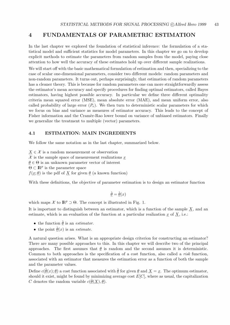
STATISTICAL METHODS FOR SIGNAL PROCESSING c©Alfred Hero 1999 43
4 FUNDAMENTALS OF PARAMETRIC ESTIMATION
In the last chapter we explored the foundation of statistical inference: the formulation of a sta-tistical model and sufficient statistics for model parameters. In this chapter we go on to developexplicit methods to estimate the parameters from random samples from the model, paying closeattention to how well the accuracy of these estimates hold up over different sample realizations.
We will start off with the basic mathematical formulation of estimation and then, specializing to thecase of scalar one-dimensional parameters, consider two different models: random parameters andnon-random parameters. It turns out, perhaps surprisingly, that estimation of random parametershas a cleaner theory. This is because for random parameters one can more straightforwardly assessthe estimator’s mean accuracy and specify procedures for finding optimal estimators, called Bayesestimators, having highest possible accuracy. In particular we define three different optimalitycriteria mean squared error (MSE), mean absolute error (MAE), and mean uniform error, alsocalled probability of large error (Pe). We then turn to deterministic scalar parameters for whichwe focus on bias and variance as measures of estimator accuracy. This leads to the concept ofFisher information and the Cramer-Rao lower bound on variance of unbiased estimators. Finallywe generalize the treatment to multiple (vector) parameters.
4.1 ESTIMATION: MAIN INGREDIENTS
We follow the same notation as in the last chapter, summarized below.
X ∈ X is a random measurement or observationX is the sample space of measurement realizations xθ ∈ Θ is an unknown parameter vector of interestΘ ⊂ IRp is the parameter spacef(x; θ) is the pdf of X for given θ (a known function)
With these definitions, the objective of parameter estimation is to design an estimator function
θ = θ(x)
which maps X to IRp ⊃ Θ. The concept is illustrated in Fig. 1.
It is important to distinguish between an estimator, which is a function of the sample X, and anestimate, which is an evaluation of the function at a particular realization x of X, i.e.:
• the function θ is an estimator.• the point θ(x) is an estimate.
A natural question arises. What is an appropriate design criterion for constructing an estimator?There are many possible approaches to this. In this chapter we will describe two of the principalapproaches. The first assumes that θ is random and the second assumes it is deterministic.Common to both approaches is the specification of a cost function, also called a risk function,associated with an estimator that measures the estimation error as a function of both the sampleand the parameter values.
Define c(θ(x); θ) a cost function associated with θ for given θ and X = x. The optimum estimator,should it exist, might be found by minimizing average cost E[C], where as usual, the capitalizationC denotes the random variable c(θ(X), θ).
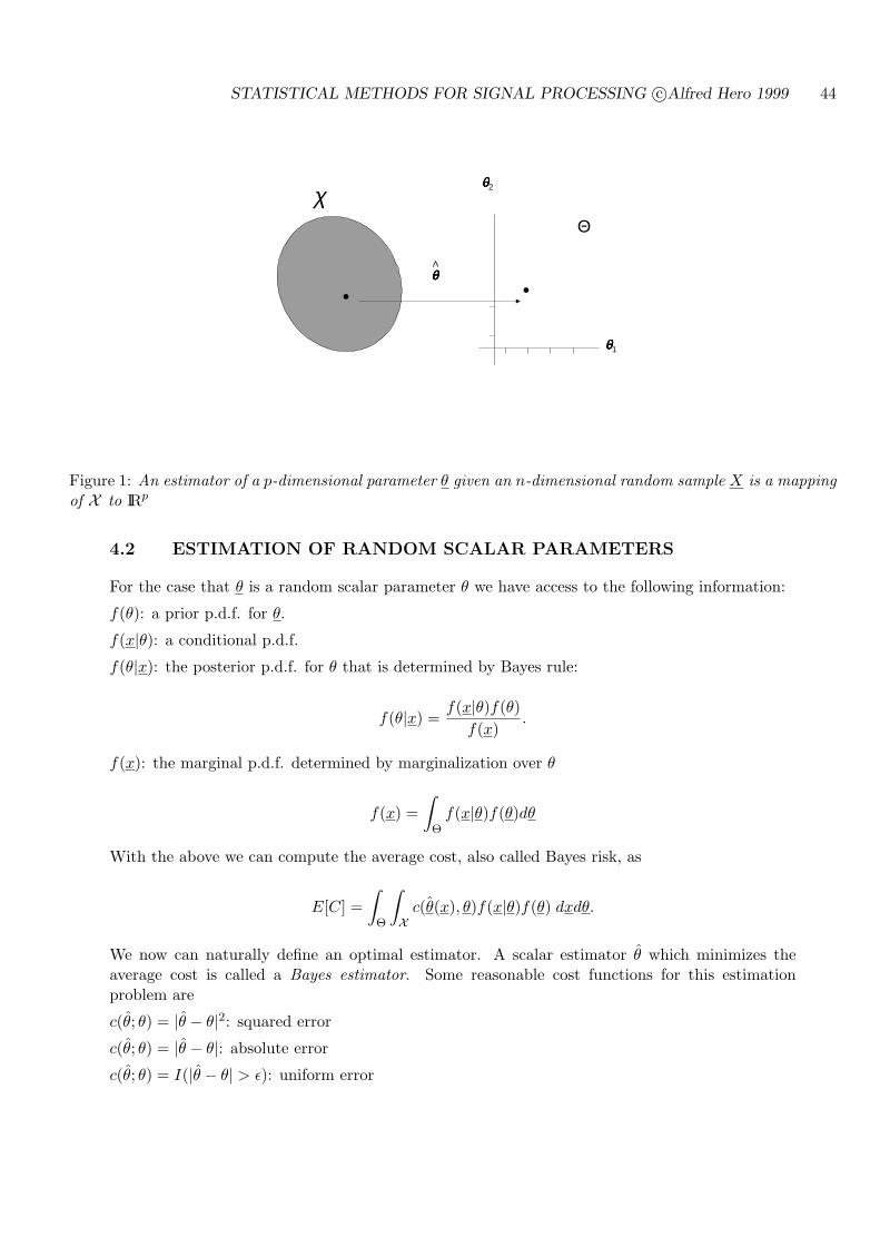
STATISTICAL METHODS FOR SIGNAL PROCESSING c©Alfred Hero 1999 44
.
χΘ
θθθθ1
θθθθ2
θθθθ^ .
Figure 1: An estimator of a p-dimensional parameter θ given an n-dimensional random sample X is a mappingof X to IRp
4.2 ESTIMATION OF RANDOM SCALAR PARAMETERS
For the case that θ is a random scalar parameter θ we have access to the following information:
f(θ): a prior p.d.f. for θ.
f(x|θ): a conditional p.d.f.
f(θ|x): the posterior p.d.f. for θ that is determined by Bayes rule:
f(θ|x) =f(x|θ)f(θ)
f(x).
f(x): the marginal p.d.f. determined by marginalization over θ
f(x) =∫
Θf(x|θ)f(θ)dθ
With the above we can compute the average cost, also called Bayes risk, as
E[C] =∫
Θ
∫
Xc(θ(x), θ)f(x|θ)f(θ) dxdθ.
We now can naturally define an optimal estimator. A scalar estimator θ which minimizes theaverage cost is called a Bayes estimator. Some reasonable cost functions for this estimationproblem are
c(θ; θ) = |θ − θ|2: squared error
c(θ; θ) = |θ − θ|: absolute error
c(θ; θ) = I(|θ − θ| > ε): uniform error
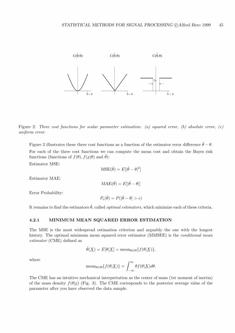
STATISTICAL METHODS FOR SIGNAL PROCESSING c©Alfred Hero 1999 45
^ ^ ^
C(^
C(^
C(^
Figure 2: Three cost functions for scalar parameter estimation: (a) squared error, (b) absolute error, (c)uniform error.
Figure 2 illustrates these three cost functions as a function of the estimator error difference θ− θ.
For each of the three cost functions we can compute the mean cost and obtain the Bayes riskfunctions (functions of f(θ), f(x|θ) and θ):
Estimator MSE:MSE(θ) = E[|θ − θ|2]
Estimator MAE:MAE(θ) = E[|θ − θ|]
Error Probability:Pe(θ) = P (|θ − θ| > ε)
It remains to find the estimators θ, called optimal estimators, which minimize each of these criteria.
4.2.1 MINIMUM MEAN SQUARED ERROR ESTIMATION
The MSE is the most widespread estimation criterion and arguably the one with the longesthistory. The optimal minimum mean squared error estimator (MMSEE) is the conditional meanestimator (CME) defined as
θ(X) = E[θ|X] = meanθ∈Θf(θ|X),
wheremeanθ∈Θf(θ|X) =
∫ ∞
−∞θf(θ|X)dθ.
The CME has an intuitive mechanical interpretation as the center of mass (1st moment of inertia)of the mass density f(θ|x) (Fig. 3). The CME corresponds to the posterior average value of theparameter after you have observed the data sample.
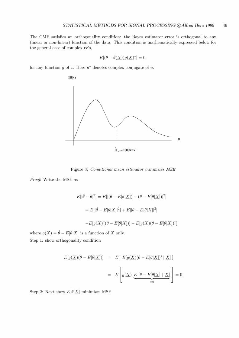
STATISTICAL METHODS FOR SIGNAL PROCESSING c©Alfred Hero 1999 46
The CME satisfies an orthogonality condition: the Bayes estimator error is orthogonal to any(linear or non-linear) function of the data. This condition is mathematically expressed below forthe general case of complex rv’s,
E[(θ − θ(X))g(X)∗] = 0,
for any function g of x. Here u∗ denotes complex conjugate of u.
f( |x)
CME E[ X=x^
Figure 3: Conditional mean estimator minimizes MSE
Proof: Write the MSE as
E[|θ − θ|2] = E[|(θ − E[θ|X])− (θ −E[θ|X])|2]
= E[|θ − E[θ|X]|2] + E[|θ − E[θ|X]|2]
−E[g(X)∗(θ − E[θ|X])]− E[g(X)(θ − E[θ|X])∗]
where g(X) = θ − E[θ|X] is a function of X only.
Step 1: show orthogonality condition
E[g(X)(θ −E[θ|X])] = E [ E[g(X)(θ − E[θ|X])∗| X] ]
= E
g(X) E [θ −E[θ|X] | X]︸ ︷︷ ︸
=0
= 0
Step 2: Next show E[θ|X] minimizes MSE
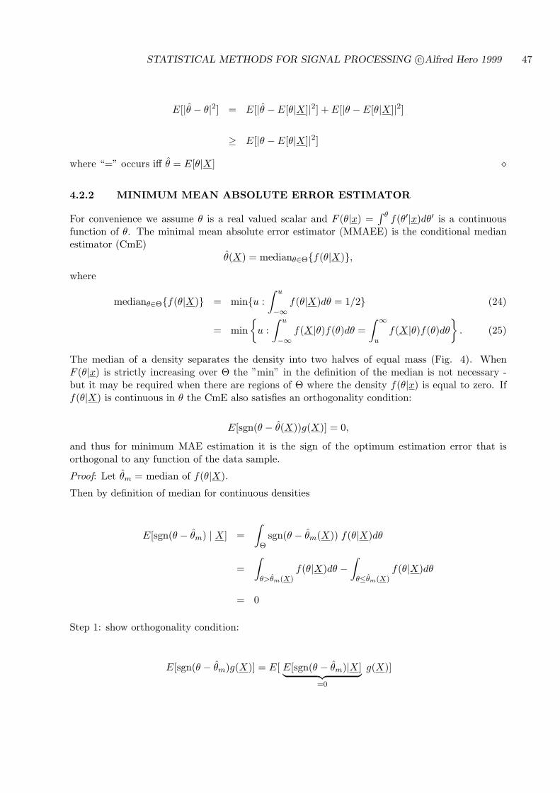
STATISTICAL METHODS FOR SIGNAL PROCESSING c©Alfred Hero 1999 47
E[|θ − θ|2] = E[|θ −E[θ|X]|2] + E[|θ −E[θ|X]|2]
≥ E[|θ −E[θ|X]|2]
where “=” occurs iff θ = E[θ|X] ¦
4.2.2 MINIMUM MEAN ABSOLUTE ERROR ESTIMATOR
For convenience we assume θ is a real valued scalar and F (θ|x) =∫ θ
f(θ′|x)dθ′ is a continuousfunction of θ. The minimal mean absolute error estimator (MMAEE) is the conditional medianestimator (CmE)
θ(X) = medianθ∈Θf(θ|X),where
medianθ∈Θf(θ|X) = minu :∫ u
−∞f(θ|X)dθ = 1/2 (24)
= min
u :∫ u
−∞f(X|θ)f(θ)dθ =
∫ ∞
uf(X|θ)f(θ)dθ
. (25)
The median of a density separates the density into two halves of equal mass (Fig. 4). WhenF (θ|x) is strictly increasing over Θ the ”min” in the definition of the median is not necessary -but it may be required when there are regions of Θ where the density f(θ|x) is equal to zero. Iff(θ|X) is continuous in θ the CmE also satisfies an orthogonality condition:
E[sgn(θ − θ(X))g(X)] = 0,
and thus for minimum MAE estimation it is the sign of the optimum estimation error that isorthogonal to any function of the data sample.
Proof: Let θm = median of f(θ|X).
Then by definition of median for continuous densities
E[sgn(θ − θm) | X] =∫
Θsgn(θ − θm(X)) f(θ|X)dθ
=∫
θ>θm(X)f(θ|X)dθ −
∫
θ≤θm(X)f(θ|X)dθ
= 0
Step 1: show orthogonality condition:
E[sgn(θ − θm)g(X)] = E[ E[sgn(θ − θm)|X]︸ ︷︷ ︸=0
g(X)]

STATISTICAL METHODS FOR SIGNAL PROCESSING c©Alfred Hero 1999 48
f( |x)
CmE
^
1/2 area
Figure 4: Conditional median estimator minimizes MAE
Step 2: for θ arbitrary we have (apply “useful formula” below)
MAE(θ) = E[| θ − θm︸ ︷︷ ︸a
+ θm − θ︸ ︷︷ ︸∆
|]
= E[|θ − θm|] + E[sgn(θ − θ)∆]︸ ︷︷ ︸=0
+E [sgn(a + ∆)− sgn(a)](a + ∆)︸ ︷︷ ︸≥[sgn(a+∆)−1](a+∆)≥0
≥ E[|θ − θm|]
Useful formula: |a + ∆| = |a|+ sgn(a)∆ + [sgn(a + ∆)− sgn(a)](a + ∆)
4.2.3 MINIMUM MEAN UNIFORM ERROR ESTIMATION
Unlike the MSE or MAE, the MUE penalizes only those errors that exceed a tolerance level ε > 0and this penalty is uniform. For small ε the optimal estimator is the maximum a posteriori (MAP)estimator, which is also called the posterior mode estimator (Fig. 5)
θ(X) = argmaxθ∈Θf(θ|X) (26)
= argmaxθ∈Θ
f(X|θ)f(θ)
f(X)
(27)
= argmaxθ∈Θf(X|θ)f(θ). (28)
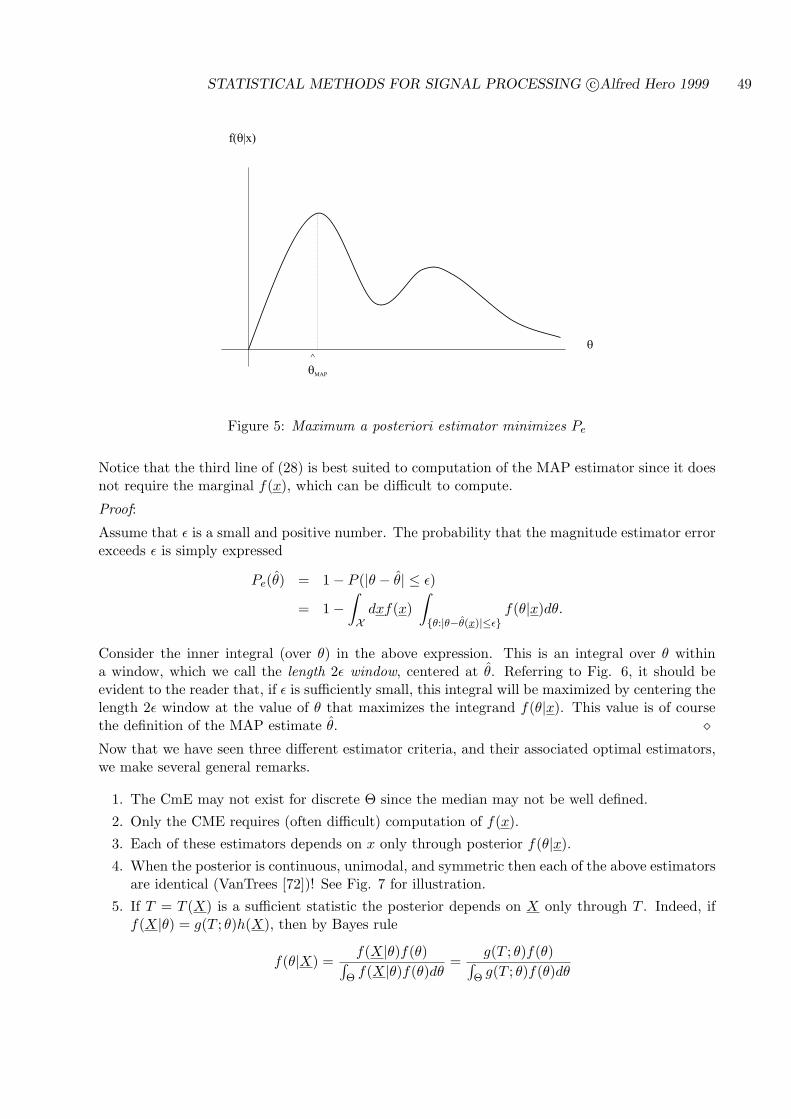
STATISTICAL METHODS FOR SIGNAL PROCESSING c©Alfred Hero 1999 49
f( |x)
MAP
^
Figure 5: Maximum a posteriori estimator minimizes Pe
Notice that the third line of (28) is best suited to computation of the MAP estimator since it doesnot require the marginal f(x), which can be difficult to compute.
Proof:
Assume that ε is a small and positive number. The probability that the magnitude estimator errorexceeds ε is simply expressed
Pe(θ) = 1− P (|θ − θ| ≤ ε)
= 1−∫
Xdxf(x)
∫
θ:|θ−θ(x)|≤εf(θ|x)dθ.
Consider the inner integral (over θ) in the above expression. This is an integral over θ withina window, which we call the length 2ε window, centered at θ. Referring to Fig. 6, it should beevident to the reader that, if ε is sufficiently small, this integral will be maximized by centering thelength 2ε window at the value of θ that maximizes the integrand f(θ|x). This value is of coursethe definition of the MAP estimate θ. ¦Now that we have seen three different estimator criteria, and their associated optimal estimators,we make several general remarks.
1. The CmE may not exist for discrete Θ since the median may not be well defined.
2. Only the CME requires (often difficult) computation of f(x).
3. Each of these estimators depends on x only through posterior f(θ|x).
4. When the posterior is continuous, unimodal, and symmetric then each of the above estimatorsare identical (VanTrees [72])! See Fig. 7 for illustration.
5. If T = T (X) is a sufficient statistic the posterior depends on X only through T . Indeed, iff(X|θ) = g(T ; θ)h(X), then by Bayes rule
f(θ|X) =f(X|θ)f(θ)∫
Θ f(X|θ)f(θ)dθ=
g(T ; θ)f(θ)∫Θ g(T ; θ)f(θ)dθ
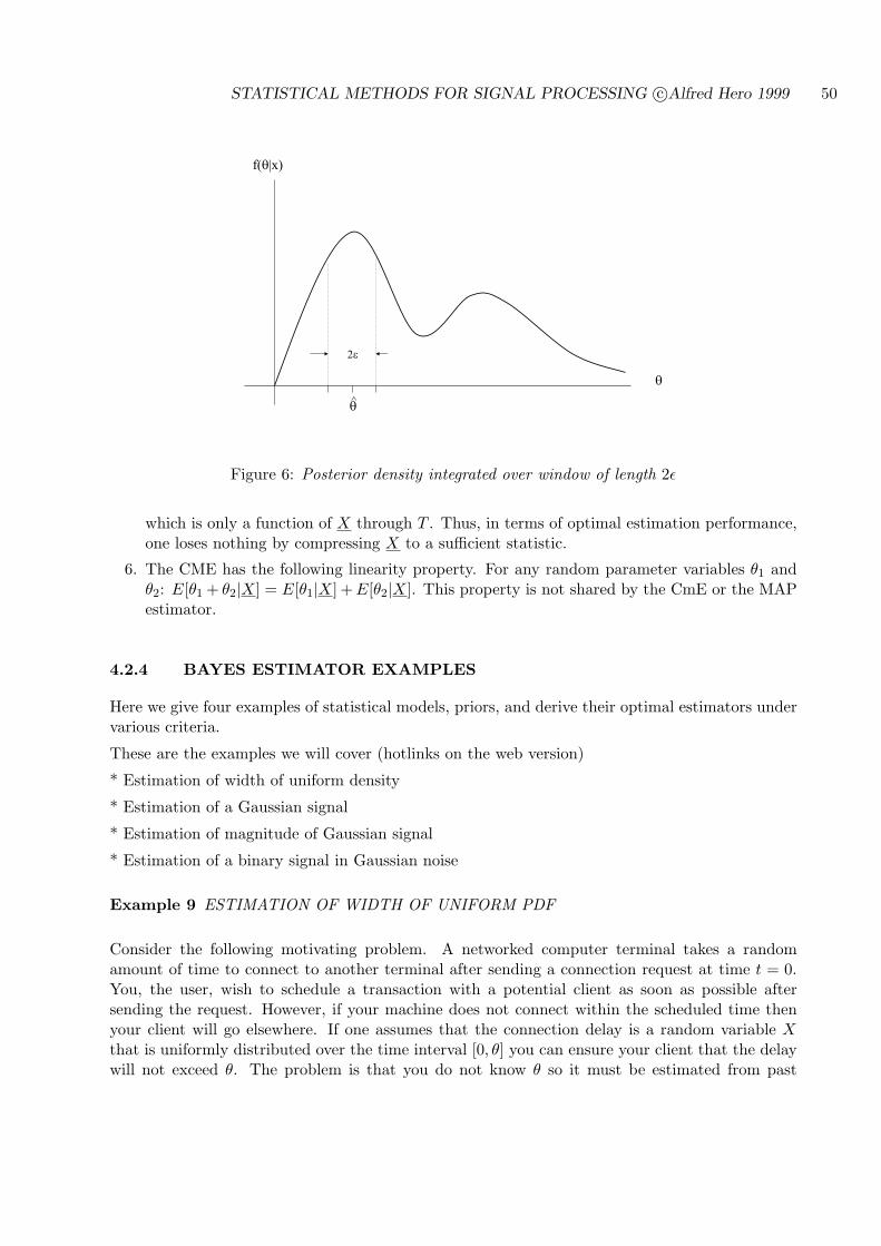
STATISTICAL METHODS FOR SIGNAL PROCESSING c©Alfred Hero 1999 50
f( |x)
^
2
Figure 6: Posterior density integrated over window of length 2ε
which is only a function of X through T . Thus, in terms of optimal estimation performance,one loses nothing by compressing X to a sufficient statistic.
6. The CME has the following linearity property. For any random parameter variables θ1 andθ2: E[θ1 + θ2|X] = E[θ1|X] + E[θ2|X]. This property is not shared by the CmE or the MAPestimator.
4.2.4 BAYES ESTIMATOR EXAMPLES
Here we give four examples of statistical models, priors, and derive their optimal estimators undervarious criteria.
These are the examples we will cover (hotlinks on the web version)
* Estimation of width of uniform density
* Estimation of a Gaussian signal
* Estimation of magnitude of Gaussian signal
* Estimation of a binary signal in Gaussian noise
Example 9 ESTIMATION OF WIDTH OF UNIFORM PDF
Consider the following motivating problem. A networked computer terminal takes a randomamount of time to connect to another terminal after sending a connection request at time t = 0.You, the user, wish to schedule a transaction with a potential client as soon as possible aftersending the request. However, if your machine does not connect within the scheduled time thenyour client will go elsewhere. If one assumes that the connection delay is a random variable Xthat is uniformly distributed over the time interval [0, θ] you can ensure your client that the delaywill not exceed θ. The problem is that you do not know θ so it must be estimated from past
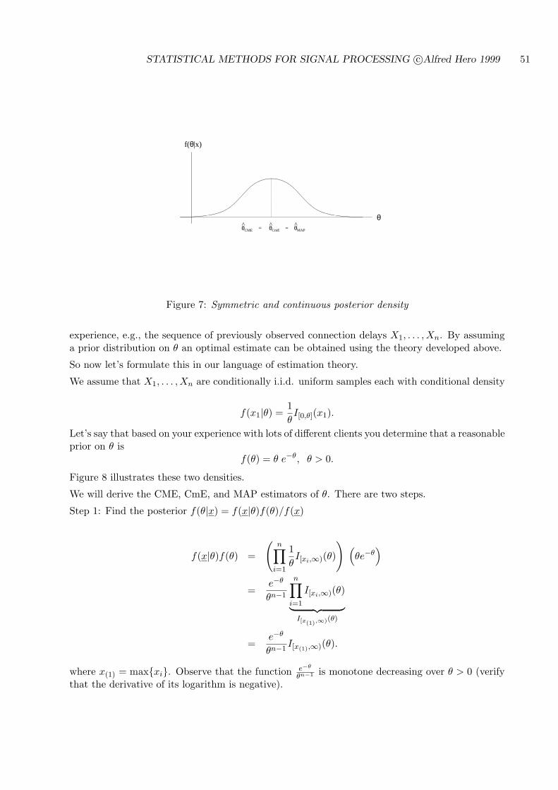
STATISTICAL METHODS FOR SIGNAL PROCESSING c©Alfred Hero 1999 51
f(θ|x)
θ θCME^ θCmE
^ θMAP^
= =
Figure 7: Symmetric and continuous posterior density
experience, e.g., the sequence of previously observed connection delays X1, . . . , Xn. By assuminga prior distribution on θ an optimal estimate can be obtained using the theory developed above.
So now let’s formulate this in our language of estimation theory.
We assume that X1, . . . , Xn are conditionally i.i.d. uniform samples each with conditional density
f(x1|θ) =1θI[0,θ](x1).
Let’s say that based on your experience with lots of different clients you determine that a reasonableprior on θ is
f(θ) = θ e−θ, θ > 0.
Figure 8 illustrates these two densities.
We will derive the CME, CmE, and MAP estimators of θ. There are two steps.
Step 1: Find the posterior f(θ|x) = f(x|θ)f(θ)/f(x)
f(x|θ)f(θ) =
(n∏
i=1
1θI[xi,∞)(θ)
) (θe−θ
)
=e−θ
θn−1
n∏
i=1
I[xi,∞)(θ)
︸ ︷︷ ︸I[x(1),∞)(θ)
=e−θ
θn−1I[x(1),∞)(θ).
where x(1) = maxxi. Observe that the function e−θ
θn−1 is monotone decreasing over θ > 0 (verifythat the derivative of its logarithm is negative).
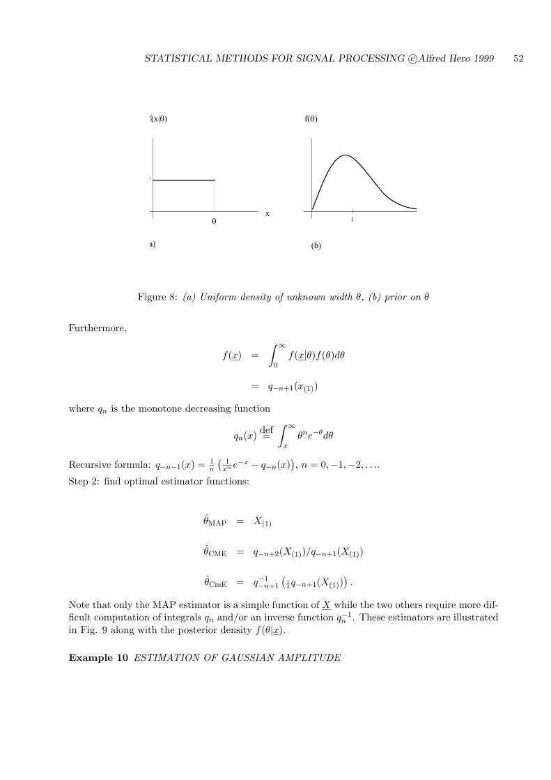
STATISTICAL METHODS FOR SIGNAL PROCESSING c©Alfred Hero 1999 52
f(x| )
x
f( )
(a) (b)
Figure 8: (a) Uniform density of unknown width θ, (b) prior on θ
Furthermore,
f(x) =∫ ∞
0f(x|θ)f(θ)dθ
= q−n+1(x(1))
where qn is the monotone decreasing function
qn(x) def=∫ ∞
xθne−θdθ
Recursive formula: q−n−1(x) = 1n
(1
xn e−x − q−n(x)), n = 0,−1,−2, . . ..
Step 2: find optimal estimator functions:
θMAP = X(1)
θCME = q−n+2(X(1))/q−n+1(X(1))
θCmE = q−1−n+1
(12q−n+1(X(1))
).
Note that only the MAP estimator is a simple function of X while the two others require more dif-ficult computation of integrals qn and/or an inverse function q−1
n . These estimators are illustratedin Fig. 9 along with the posterior density f(θ|x).
Example 10 ESTIMATION OF GAUSSIAN AMPLITUDE
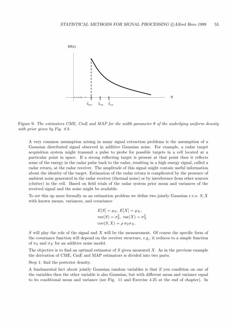
STATISTICAL METHODS FOR SIGNAL PROCESSING c©Alfred Hero 1999 53
f( |x)
x x x xx x x
MAP^
CME^
CmE^
Figure 9: The estimators CME, CmE and MAP for the width parameter θ of the underlying uniform densitywith prior given by Fig. 8.b.
A very common assumption arising in many signal extraction problems is the assumption of aGaussian distributed signal observed in additive Gaussian noise. For example, a radar targetacquisition system might transmit a pulse to probe for possible targets in a cell located at aparticular point in space. If a strong reflecting target is present at that point then it reflectssome of the energy in the radar pulse back to the radar, resulting in a high energy signal, called aradar return, at the radar receiver. The amplitude of this signal might contain useful informationabout the identity of the target. Estimation of the radar return is complicated by the presence ofambient noise generated in the radar receiver (thermal noise) or by interference from other sources(clutter) in the cell. Based on field trials of the radar system prior mean and variances of thereceived signal and the noise might be available.
To set this up more formally as an estimation problem we define two jointly Gaussian r.v.s: S,Xwith known means, variances, and covariance
E[S] = µS , E[X] = µX ,
var(S) = σ2S , var(X) = σ2
X
cov(S,X) = ρ σSσX .
S will play the role of the signal and X will be the measurement. Of course the specific form ofthe covariance function will depend on the receiver structure, e.g., it reduces to a simple functionof σS and σX for an additive noise model.
The objective is to find an optimal estimator of S given measured X. As in the previous examplethe derivation of CME, CmE and MAP estimators is divided into two parts.
Step 1: find the posterior density.
A fundamental fact about jointly Gaussian random variables is that if you condition on one ofthe variables then the other variable is also Gaussian, but with different mean and variance equalto its conditional mean and variance (see Fig. 11 and Exercise 4.25 at the end of chapter). In
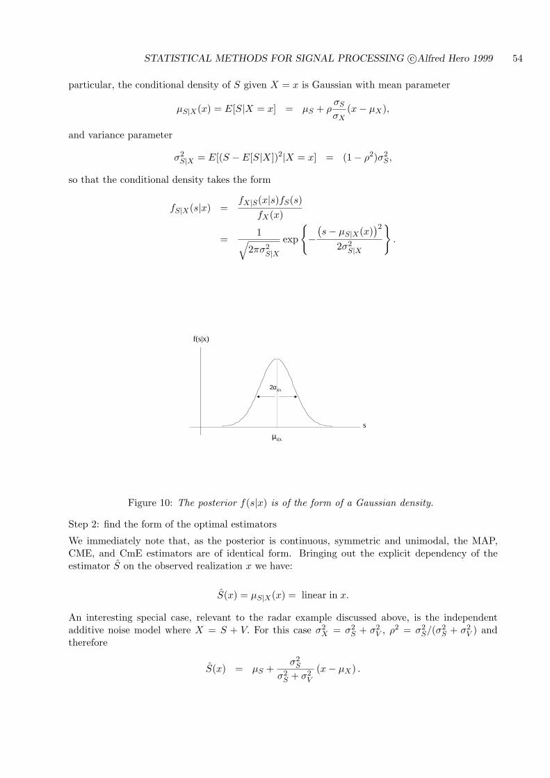
STATISTICAL METHODS FOR SIGNAL PROCESSING c©Alfred Hero 1999 54
particular, the conditional density of S given X = x is Gaussian with mean parameter
µS|X(x) = E[S|X = x] = µS + ρσS
σX(x− µX),
and variance parameter
σ2S|X = E[(S −E[S|X])2|X = x] = (1− ρ2)σ2
S ,
so that the conditional density takes the form
fS|X(s|x) =fX|S(x|s)fS(s)
fX(x)
=1√
2πσ2S|X
exp
−
(s− µS|X(x)
)2
2σ2S|X
.
f(s|x)
s
µs|x
2σs|x
Figure 10: The posterior f(s|x) is of the form of a Gaussian density.
Step 2: find the form of the optimal estimators
We immediately note that, as the posterior is continuous, symmetric and unimodal, the MAP,CME, and CmE estimators are of identical form. Bringing out the explicit dependency of theestimator S on the observed realization x we have:
S(x) = µS|X(x) = linear in x.
An interesting special case, relevant to the radar example discussed above, is the independentadditive noise model where X = S + V. For this case σ2
X = σ2S + σ2
V , ρ2 = σ2S/(σ2
S + σ2V ) and
therefore
S(x) = µS +σ2
S
σ2S + σ2
V
(x− µX) .
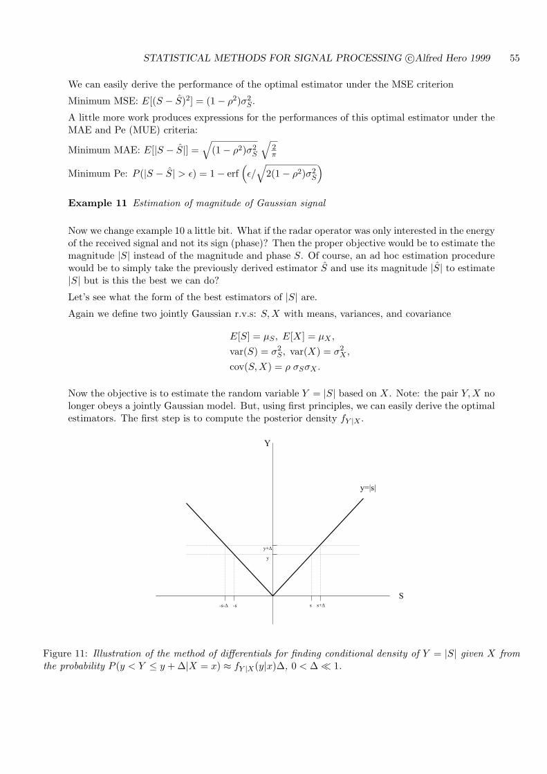
STATISTICAL METHODS FOR SIGNAL PROCESSING c©Alfred Hero 1999 55
We can easily derive the performance of the optimal estimator under the MSE criterion
Minimum MSE: E[(S − S)2] = (1− ρ2)σ2S .
A little more work produces expressions for the performances of this optimal estimator under theMAE and Pe (MUE) criteria:
Minimum MAE: E[|S − S|] =√
(1− ρ2)σ2S
√2π
Minimum Pe: P (|S − S| > ε) = 1− erf(ε/
√2(1− ρ2)σ2
S
)
Example 11 Estimation of magnitude of Gaussian signal
Now we change example 10 a little bit. What if the radar operator was only interested in the energyof the received signal and not its sign (phase)? Then the proper objective would be to estimate themagnitude |S| instead of the magnitude and phase S. Of course, an ad hoc estimation procedurewould be to simply take the previously derived estimator S and use its magnitude |S| to estimate|S| but is this the best we can do?
Let’s see what the form of the best estimators of |S| are.
Again we define two jointly Gaussian r.v.s: S, X with means, variances, and covariance
E[S] = µS , E[X] = µX ,
var(S) = σ2S , var(X) = σ2
X ,
cov(S, X) = ρ σSσX .
Now the objective is to estimate the random variable Y = |S| based on X. Note: the pair Y,X nolonger obeys a jointly Gaussian model. But, using first principles, we can easily derive the optimalestimators. The first step is to compute the posterior density fY |X .
S
y=|s|
y
y+
-s- -s s s+
Y
Figure 11: Illustration of the method of differentials for finding conditional density of Y = |S| given X fromthe probability P (y < Y ≤ y + ∆|X = x) ≈ fY |X(y|x)∆, 0 < ∆ ¿ 1.

STATISTICAL METHODS FOR SIGNAL PROCESSING c©Alfred Hero 1999 56
Since we know fS|X from the previous example this is a simple transformation of variables problemof elementary probability. We use the method of differentials (see Fig. 11) to obtain the followingrelation, valid for small ∆
fY |X(y|x)∆ = fS|X(y|x)∆ + fS|X(−y|x)∆, y ≥ 0,
or more explicitly
fY |X(y|x) =
1√2πσ2
S|X
(exp
−
(y − µS|X(x)
)2
2σ2S|X
+ exp
−
(y + µS|X(x)
)2
2σ2S|X
)I[0,∞)(y). (29)
f(y|x)
y−µs|x µs|x
Figure 12: Posterior density of Y = |S| given X
Unlike Example 10 this posterior density, shown in Fig. 12 is no longer symmetric in y. Hence weexpect the CME, CmE, and MAP estimators to be different.
The CME can be derived in explicit closed form by integration over y ∈ [0,∞) of the functionyfY |X(y|x) specified in (29)
YCME(x) = E[Y |X = x] =∣∣µS|X(x)
∣∣ erf
(|µS|X(x)|σS|X
√2
)+
√2π
σS|X e−µ2
S/2σ2S|X .
On the other hand, by investigating the MMAE equation∫∞Y fY |X(y|x)dy =
∫ Y0 fY |X(y|x)dy it is
easily seen that the CmE can only be implicitly given as the solution Y = YCmE of the following
erf
(Y − µS|X(x)
σS|X√
2
)+ erf
(Y + µS|X(x)
σS|X√
2
)=
12.
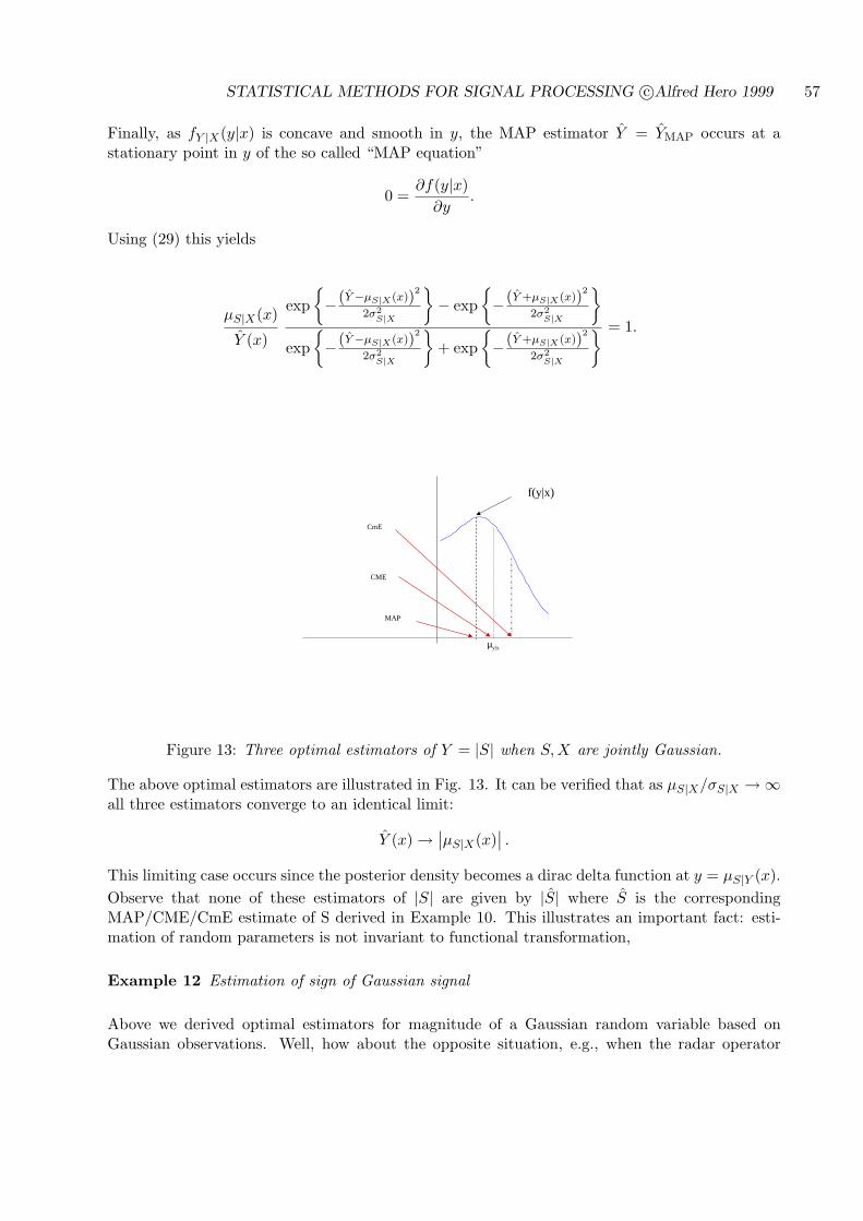
STATISTICAL METHODS FOR SIGNAL PROCESSING c©Alfred Hero 1999 57
Finally, as fY |X(y|x) is concave and smooth in y, the MAP estimator Y = YMAP occurs at astationary point in y of the so called “MAP equation”
0 =∂f(y|x)
∂y.
Using (29) this yields
µS|X(x)
Y (x)
exp−(Y−µS|X(x))2
2σ2S|X
− exp
−(Y +µS|X(x))2
2σ2S|X
exp−(Y−µS|X(x))2
2σ2S|X
+ exp
−(Y +µS|X(x))2
2σ2S|X
= 1.
f(y|x)
µy|x
MAP
CME
CmE
Figure 13: Three optimal estimators of Y = |S| when S, X are jointly Gaussian.
The above optimal estimators are illustrated in Fig. 13. It can be verified that as µS|X/σS|X →∞all three estimators converge to an identical limit:
Y (x) → ∣∣µS|X(x)∣∣ .
This limiting case occurs since the posterior density becomes a dirac delta function at y = µS|Y (x).Observe that none of these estimators of |S| are given by |S| where S is the correspondingMAP/CME/CmE estimate of S derived in Example 10. This illustrates an important fact: esti-mation of random parameters is not invariant to functional transformation,
Example 12 Estimation of sign of Gaussian signal
Above we derived optimal estimators for magnitude of a Gaussian random variable based onGaussian observations. Well, how about the opposite situation, e.g., when the radar operator
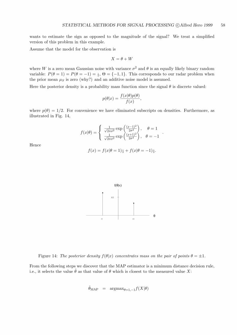
STATISTICAL METHODS FOR SIGNAL PROCESSING c©Alfred Hero 1999 58
wants to estimate the sign as opposed to the magnitude of the signal? We treat a simplifiedversion of this problem in this example.
Assume that the model for the observation is
X = θ + W
where W is a zero mean Gaussian noise with variance σ2 and θ is an equally likely binary randomvariable: P (θ = 1) = P (θ = −1) = 1
2 , Θ = −1, 1. This corresponds to our radar problem whenthe prior mean µS is zero (why?) and an additive noise model is assumed.
Here the posterior density is a probability mass function since the signal θ is discrete valued:
p(θ|x) =f(x|θ)p(θ)
f(x),
where p(θ) = 1/2. For convenience we have eliminated subscripts on densities. Furthermore, asillustrated in Fig. 14,
f(x|θ) =
1√2πσ2
exp(
(x−1)2
2σ2
), θ = 1
1√2πσ2
exp(
(x+1)2
2σ2
), θ = −1
.
Hencef(x) = f(x|θ = 1) 1
2 + f(x|θ = −1) 12 .
f(θ|x)
θ
1/2
+1-1
Figure 14: The posterior density f(θ|x) concentrates mass on the pair of points θ = ±1.
From the following steps we discover that the MAP estimator is a minimum distance decision rule,i.e., it selects the value θ as that value of θ which is closest to the measured value X:
θMAP = argmaxθ=1,−1f(X|θ)
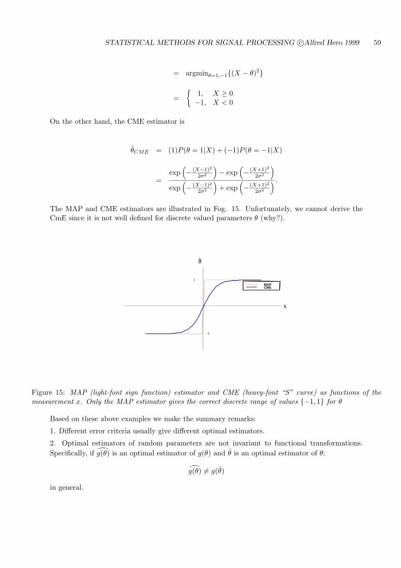
STATISTICAL METHODS FOR SIGNAL PROCESSING c©Alfred Hero 1999 59
= argminθ=1,−1(X − θ)2
=
1, X ≥ 0−1, X < 0
On the other hand, the CME estimator is
θCME = (1)P (θ = 1|X) + (−1)P (θ = −1|X)
=exp
(− (X−1)2
2σ2
)− exp
(− (X+1)2
2σ2
)
exp(− (X−1)2
2σ2
)+ exp
(− (X+1)2
2σ2
) .
The MAP and CME estimators are illustrated in Fog. 15. Unfortunately, we cannot derive theCmE since it is not well defined for discrete valued parameters θ (why?).
MAPCME
x
θ
1
-1
Figure 15: MAP (light-font sign function) estimator and CME (heavy-font “S” curve) as functions of themeasurement x. Only the MAP estimator gives the correct discrete range of values −1, 1 for θ
Based on these above examples we make the summary remarks:
1. Different error criteria usually give different optimal estimators.
2. Optimal estimators of random parameters are not invariant to functional transformations.Specifically, if g(θ) is an optimal estimator of g(θ) and θ is an optimal estimator of θ:
g(θ) 6= g(θ)
in general.
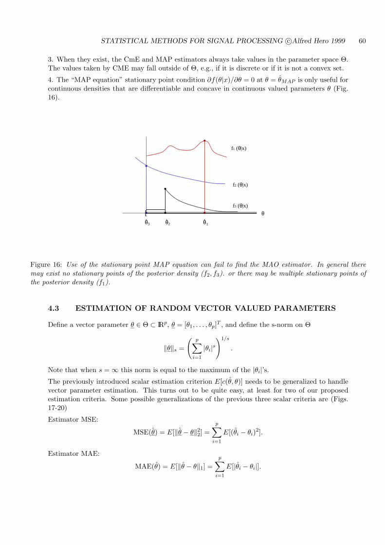
STATISTICAL METHODS FOR SIGNAL PROCESSING c©Alfred Hero 1999 60
3. When they exist, the CmE and MAP estimators always take values in the parameter space Θ.The values taken by CME may fall outside of Θ, e.g., if it is discrete or if it is not a convex set.
4. The “MAP equation” stationary point condition ∂f(θ|x)/∂θ = 0 at θ = θMAP is only useful forcontinuous densities that are differentiable and concave in continuous valued parameters θ (Fig.16).
θ
f1 (θ|x)
f2 (θ|x)
θ
θ
θ
[ f3 (θ|x)
123
Figure 16: Use of the stationary point MAP equation can fail to find the MAO estimator. In general theremay exist no stationary points of the posterior density (f2, f3). or there may be multiple stationary points ofthe posterior density (f1).
4.3 ESTIMATION OF RANDOM VECTOR VALUED PARAMETERS
Define a vector parameter θ ∈ Θ ⊂ IRp, θ = [θ1, . . . , θp]T , and define the s-norm on Θ
‖θ‖s =
(p∑
i=1
|θi|s)1/s
.
Note that when s = ∞ this norm is equal to the maximum of the |θi|’s.The previously introduced scalar estimation criterion E[c(θ, θ)] needs to be generalized to handlevector parameter estimation. This turns out to be quite easy, at least for two of our proposedestimation criteria. Some possible generalizations of the previous three scalar criteria are (Figs.17-20)
Estimator MSE:
MSE(θ) = E[‖θ − θ‖22] =
p∑
i=1
E[(θi − θi)2].
Estimator MAE:
MAE(θ) = E[‖θ − θ‖1] =p∑
i=1
E[|θi − θi|].
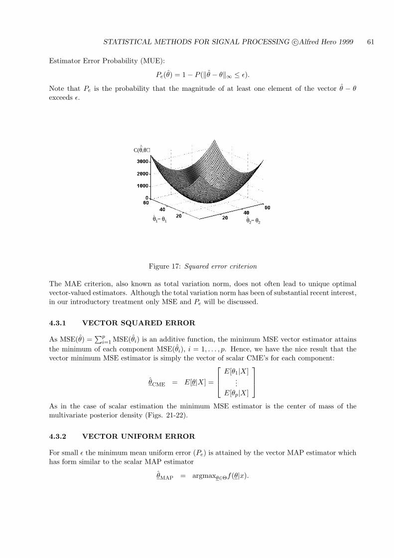
STATISTICAL METHODS FOR SIGNAL PROCESSING c©Alfred Hero 1999 61
Estimator Error Probability (MUE):
Pe(θ) = 1− P (‖θ − θ‖∞ ≤ ε).
Note that Pe is the probability that the magnitude of at least one element of the vector θ − θexceeds ε.
C(θ,θ)^
θ1− θ1^
θ2− θ2^
Figure 17: Squared error criterion
The MAE criterion, also known as total variation norm, does not often lead to unique optimalvector-valued estimators. Although the total variation norm has been of substantial recent interest,in our introductory treatment only MSE and Pe will be discussed.
4.3.1 VECTOR SQUARED ERROR
As MSE(θ) =∑p
i=1 MSE(θi) is an additive function, the minimum MSE vector estimator attainsthe minimum of each component MSE(θi), i = 1, . . . , p. Hence, we have the nice result that thevector minimum MSE estimator is simply the vector of scalar CME’s for each component:
θCME = E[θ|X] =
E[θ1|X]...
E[θp|X]
As in the case of scalar estimation the minimum MSE estimator is the center of mass of themultivariate posterior density (Figs. 21-22).
4.3.2 VECTOR UNIFORM ERROR
For small ε the minimum mean uniform error (Pe) is attained by the vector MAP estimator whichhas form similar to the scalar MAP estimator
θMAP = argmaxθ∈Θf(θ|x).

STATISTICAL METHODS FOR SIGNAL PROCESSING c©Alfred Hero 1999 62
Figure 18: Absolute error criterion
Figure 19: Uniform error criterion
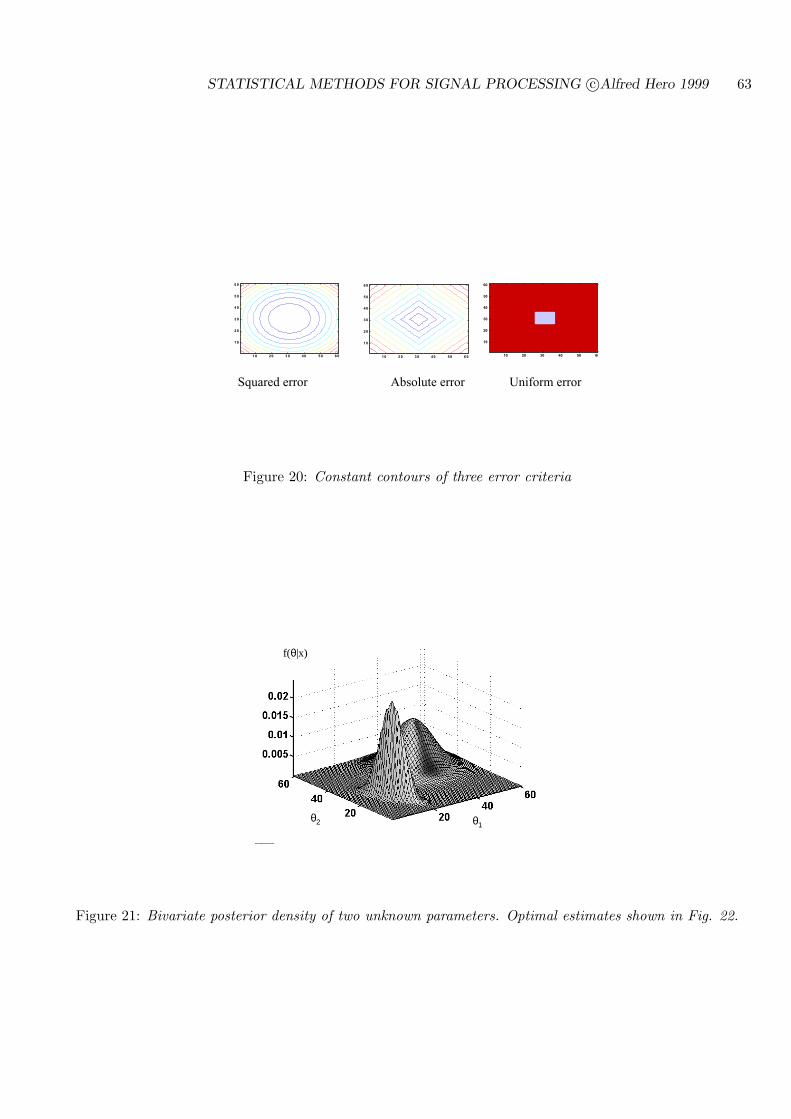
STATISTICAL METHODS FOR SIGNAL PROCESSING c©Alfred Hero 1999 63
10 20 30 40 50 60
10
20
30
40
50
60
10 20 30 40 50 60
10
20
30
40
50
60
10 20 30 40 50 60
10
20
30
40
50
60
Squared error Absolute error Uniform error
Figure 20: Constant contours of three error criteria
f(θ|x)
θ1θ2
Figure 21: Bivariate posterior density of two unknown parameters. Optimal estimates shown in Fig. 22.
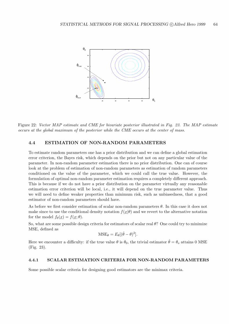
STATISTICAL METHODS FOR SIGNAL PROCESSING c©Alfred Hero 1999 64
20 30 40 50
20
30
40
50
θ1
θ2
..
θCME^
θMAP^
Figure 22: Vector MAP estimate and CME for bivariate posterior illustrated in Fig. 23. The MAP estimateoccurs at the global maximum of the posterior while the CME occurs at the center of mass.
4.4 ESTIMATION OF NON-RANDOM PARAMETERS
To estimate random parameters one has a prior distribution and we can define a global estimationerror criterion, the Bayes risk, which depends on the prior but not on any particular value of theparameter. In non-random parameter estimation there is no prior distribution. One can of courselook at the problem of estimation of non-random parameters as estimation of random parametersconditioned on the value of the parameter, which we could call the true value. However, theformulation of optimal non-random parameter estimation requires a completely different approach.This is because if we do not have a prior distribution on the parameter virtually any reasonableestimation error criterion will be local, i.e., it will depend on the true parameter value. Thuswe will need to define weaker properties than minimum risk, such as unbiasedness, that a goodestimator of non-random parameters should have.
As before we first consider estimation of scalar non-random parameters θ. In this case it does notmake since to use the conditional density notation f(x|θ) and we revert to the alternative notationfor the model fθ(x) = f(x; θ).
So, what are some possible design criteria for estimators of scalar real θ? One could try to minimizeMSE, defined as
MSEθ = Eθ[(θ − θ)2].
Here we encounter a difficulty: if the true value θ is θ0, the trivial estimator θ = θo attains 0 MSE(Fig. 23).
4.4.1 SCALAR ESTIMATION CRITERIA FOR NON-RANDOM PARAMETERS
Some possible scalar criteria for designing good estimators are the minimax criteria.

STATISTICAL METHODS FOR SIGNAL PROCESSING c©Alfred Hero 1999 65
ΜSEθ
θθo
Figure 23: MSE curve as function of θ for trivial estimator θ = θo of non-random parameter.
1. Minimize worst case MSE. Choose θ to minimize
maxθ
MSEθ(θ) = maxθ
Eθ[(θ − θ)2]
2. Minimize worst case estimator error probability:
maxθ
Pe = maxθ
Pθ(|θ − θ| > ε)
If we would be satisfied by minimizing an upper bound on maxPe, then we could invoke Tchebychevinequality
Pθ(|θ − θ| ≥ ε) ≤ Eθ[|θ − θ|2]ε2
(30)
and focus on minimizing the worst case MSE. There is a large literature on minimax MSE esti-mation, see for example [39], but the mathematical level necessary to develop this theory is tooadvanced for an introductory treatment. We will not consider minimax estimation further in thisbook.
We next give several weaker conditions that a good estimator should satisfy, namely consistencyand unbiasedness.
Definition: θn = θ(X1, . . . , Xn) is said to be (weakly) consistent if for all θ and all ε > 0
limn→∞Pθ(|θn − θ| > ε) = 0
This means that θn converges in probability to the true parameter θ. It also means that the pdfof the estimator concentrates about θ (Fig. 24). Furthermore, by the Tchebychev inequality (30),if MSE goes to zero as n →∞ then θn is consistent. As the MSE is usually easier to derive than
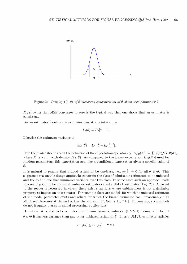
STATISTICAL METHODS FOR SIGNAL PROCESSING c©Alfred Hero 1999 66
^ f(θ; θ)
θ
2ε
θ
Figure 24: Density f(θ; θ) of θ measures concentration of θ about true parameter θ
Pe, showing that MSE converges to zero is the typical way that one shows that an estimator isconsistent.
For an estimator θ define the estimator bias at a point θ to be
bθ(θ) = Eθ[θ]− θ.
Likewise the estimator variance is
varθ(θ) = Eθ[(θ −Eθ[θ])2].
Here the reader should recall the definition of the expectation operator Eθ: Eθ[g(X)] =∫X g(x)f(x; θ)dx,
where X is a r.v. with density f(x; θ). As compared to the Bayes expectation E[g(X)] used forrandom parameters, this expectation acts like a conditional expectation given a specific value ofθ.
It is natural to require that a good estimator be unbiased, i.e., bθ(θ) = 0 for all θ ∈ Θ. Thissuggests a reasonable design approach: constrain the class of admissible estimators to be unbiasedand try to find one that minimizes variance over this class. In some cases such an approach leadsto a really good, in fact optimal, unbiased estimator called a UMVU estimator (Fig. 25). A caveatto the reader is necessary however: there exist situations where unbiasedness is not a desirableproperty to impose on an estimator. For example there are models for which no unbiased estimatorof the model parameter exists and others for which the biased estimator has unreasonably highMSE, see Exercises at the end of this chapter and [57, Sec. 7.11, 7.15]. Fortunately, such modelsdo not frequently arise in signal processing applications.
Definition: θ is said to be a uniform minimum variance unbiased (UMVU) estimator if for all
θ ∈ Θ it has less variance than any other unbiased estimator ˆθ. Thus a UMVU estimator satisfies
varθ(θ) ≤ varθ(ˆθ), θ ∈ Θ
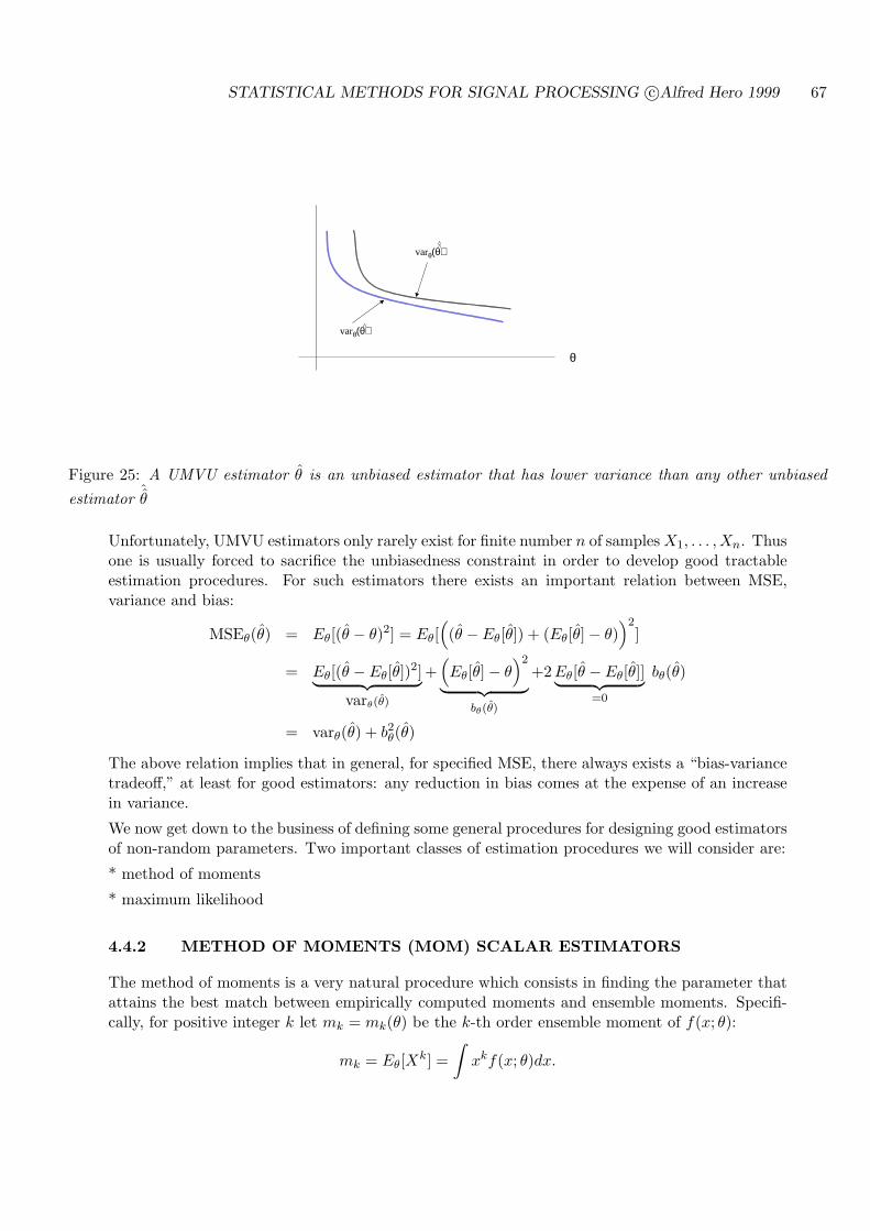
STATISTICAL METHODS FOR SIGNAL PROCESSING c©Alfred Hero 1999 67
θ
varθ(θ)^
varθ(θ)^
^
Figure 25: A UMVU estimator θ is an unbiased estimator that has lower variance than any other unbiasedestimator ˆ
θ
Unfortunately, UMVU estimators only rarely exist for finite number n of samples X1, . . . , Xn. Thusone is usually forced to sacrifice the unbiasedness constraint in order to develop good tractableestimation procedures. For such estimators there exists an important relation between MSE,variance and bias:
MSEθ(θ) = Eθ[(θ − θ)2] = Eθ[((θ − Eθ[θ]) + (Eθ[θ]− θ)
)2]
= Eθ[(θ −Eθ[θ])2]︸ ︷︷ ︸varθ(θ)
+(Eθ[θ]− θ
)2
︸ ︷︷ ︸bθ(θ)
+2 Eθ[θ − Eθ[θ]]︸ ︷︷ ︸=0
bθ(θ)
= varθ(θ) + b2θ(θ)
The above relation implies that in general, for specified MSE, there always exists a “bias-variancetradeoff,” at least for good estimators: any reduction in bias comes at the expense of an increasein variance.
We now get down to the business of defining some general procedures for designing good estimatorsof non-random parameters. Two important classes of estimation procedures we will consider are:
* method of moments
* maximum likelihood
4.4.2 METHOD OF MOMENTS (MOM) SCALAR ESTIMATORS
The method of moments is a very natural procedure which consists in finding the parameter thatattains the best match between empirically computed moments and ensemble moments. Specifi-cally, for positive integer k let mk = mk(θ) be the k-th order ensemble moment of f(x; θ):
mk = Eθ[Xk] =∫
xkf(x; θ)dx.
STATISTICAL METHODS FOR SIGNAL PROCESSING c©Alfred Hero 1999 68
What if we could find a set of K moments such that some vector function h could be found thatsatisfies
θ = h(m1(θ), . . . , mK(θ)).
For example, let’s say we could compute a closed form expression g(θ) for the k-th ensemblemoment Eθ[Xk] and found that the function g was invertible. Then if someone only reported thevalue mk of this ensemble moment without specifying the θ for which it was computed we couldrecover θ by applying the inverse function
θ = g−1(mk).
Since g−1 recovers θ from the ensemble moment of X, if we only have access to an i.i.d. sampleX1, . . . , Xn from f(x; θ) it makes sense to estimate θ by applying g−1 to an estimated momentsuch as the empirical average
mk =1n
n∑
i=1
Xki ,
yielding the estimatorθ = g−1(mk).
In many cases it is difficult to find a single ensemble moment that gives an invertible functionof θ. Indeed, using only the k-th moment we may only be able to find a constraint equationg(θ) = mk that gives several possible solutions θ. In these cases, one can sometimes computeother ensemble and empirical moments to construct more constraint equations and force a uniquesolution. We will explore this approach in the examples below. Next we give some importantasymptotic optimality properties of MOM estimators (see Serfling [61] for proofs).
IMPORTANT PROPERTIES OF MOM ESTIMATORS
When the moments mk are smooth functions of the parameter θ and an inverse function g−1,described above, exists:
1. MOM estimators are asymptotically unbiased as n →∞2. MOM estimators are consistent
Note that MOM estimators are not always unbiased in the finite sample regime. There are, how-ever, some inherent difficulties that one sometimes encounters with MOM which are summarizedbelow.
1. MOM estimator is not unique, i.e., it depends on what order moment is used.
2. MOM is inapplicable in cases where moments do not exist (e.g. Cauchy p.d.f.) or are unstable.
An alternative to MOM which can sometimes circumvent the existence problem is to match sampleand ensemble fractional moments mk where k is a positive rational number less than one. Fractionalmoments can exist when integer moments do not exist and can be quite useful in these situations[62].
Let’s do some examples.
Example 13 X i.i.d. Bernoulli random variables
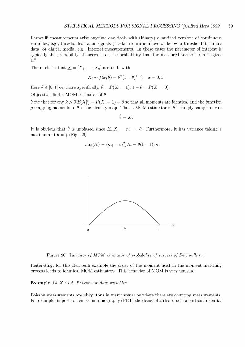
STATISTICAL METHODS FOR SIGNAL PROCESSING c©Alfred Hero 1999 69
Bernoulli measurements arise anytime one deals with (binary) quantized versions of continuousvariables, e.g., thresholded radar signals (”radar return is above or below a threshold”), failuredata, or digital media, e.g., Internet measurements. In these cases the parameter of interest istypically the probability of success, i.e., the probability that the measured variable is a ”logical1.”
The model is that X = [X1, . . . , Xn] are i.i.d. with
Xi ∼ f(x; θ) = θx(1− θ)1−x, x = 0, 1.
Here θ ∈ [0, 1] or, more specifically, θ = P (Xi = 1), 1− θ = P (Xi = 0).
Objective: find a MOM estimator of θ
Note that for any k > 0 E[Xki ] = P (Xi = 1) = θ so that all moments are identical and the function
g mapping moments to θ is the identity map. Thus a MOM estimator of θ is simply sample mean:
θ = X.
It is obvious that θ is unbiased since Eθ[X] = m1 = θ. Furthermore, it has variance taking amaximum at θ = 1
2 (Fig. 26)
varθ(X) = (m2 −m21)/n = θ(1− θ)/n.
1/2 10θ
Figure 26: Variance of MOM estimator of probability of success of Bernoulli r.v.
Reiterating, for this Bernoulli example the order of the moment used in the moment matchingprocess leads to identical MOM estimators. This behavior of MOM is very unusual.
Example 14 X i.i.d. Poisson random variables
Poisson measurements are ubiquitous in many scenarios where there are counting measurements.For example, in positron emission tomography (PET) the decay of an isotope in a particular spatial
STATISTICAL METHODS FOR SIGNAL PROCESSING c©Alfred Hero 1999 70
location within a patient’s body produces a gamma ray which is registered as a single ”count” ona detector. The temporal record of the times at which these counts are registered on the detectorforms a Poisson process [64]. The total number of counts registered over a finite time intervalis a Poisson random variable with rate parameter determined by the mean concentration of theisotope. The objective of a PET system is to reconstruct, i.e., estimate, the distribution of ratesover the imaging volume. The Poisson distribution is also frequently used as a model for thenumber of components or degrees of freedom generating the measured values. For example, thenumber of molecules in a mass spectroscopy measurement, the number of atoms in a molecule, orthe number of targets in a cell detected by a radar.
Again assuming i.i.d. measurements, the model for each data sample is
Xi ∼ p(x; θ) =θx
x!e−θ, x = 0, 1, 2, . . . ,
where θ > 0 is the unknown rate. It is readily verified that the mean m1 is equal to θ. Therefore,like in the Bernoulli example a MOM estimator of θ is the sample mean
θ1 = X.
Alternatively, as the second moment satisfies m2 = θ+θ2, another MOM estimator is the (positive)value of θ2 which satisfies the equation : θ2 + θ2
2 = 1n
∑ni=1 X2
i := X2, i.e.
θ2 =−1±
√1 + 4X2
2.
As yet another example, we can express m2 as m2 = θ + m21 or θ = m2 −m2
1 = varθ(Xi). Hence,a MOM estimator is
θ3 = X2 −X2 = n−1
n∑
i=1
(Xi −X)2.
Among all of these MOM estimators only the sample mean estimator is unbiased for finite n:
Eθ(θ1) = θ, varθ(θ1) = θ/n,
Eθ(θ3) =n− 1
nθ, varθ(θ3) ≈ (2θ2 + θ)/n.
Closed form expressions for bias and variance of θ2 do not exist.
You should notice that θ1 compares favorably to θ3 since it has both lower bias and lower variance.
We make the following observations.
1. θ1 is unbiased for all n.
2. θ2, θ3 are asymptotically unbiased as n →∞.
3. Consistency of θ1 and θ3 is directly verifiable from the above expressions for mean and varianceand Thebychev’s inequality.
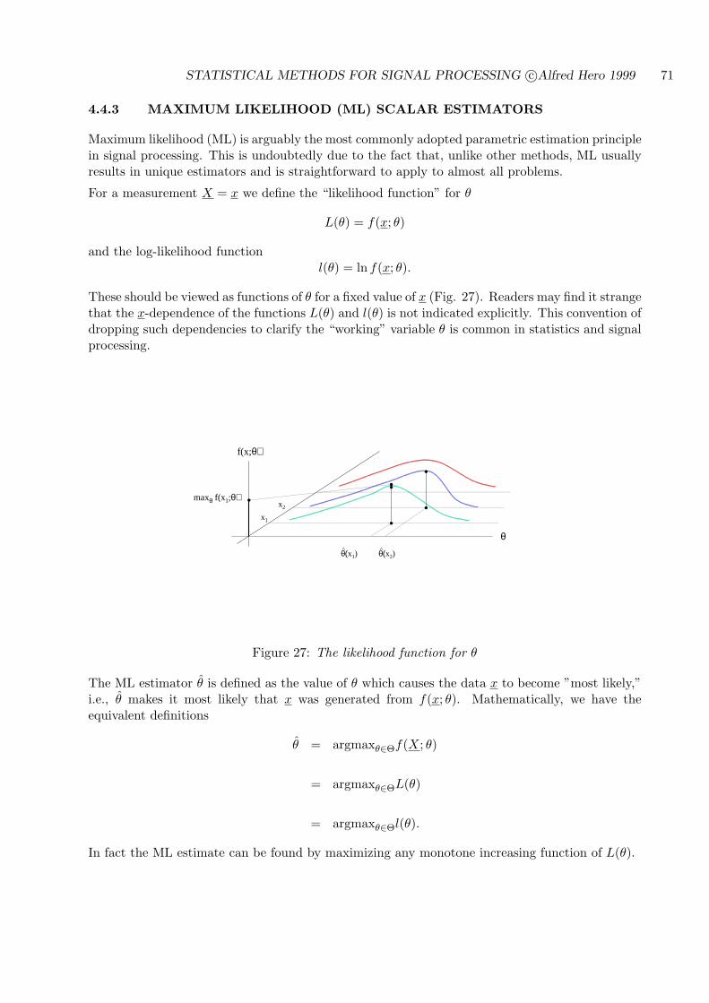
STATISTICAL METHODS FOR SIGNAL PROCESSING c©Alfred Hero 1999 71
4.4.3 MAXIMUM LIKELIHOOD (ML) SCALAR ESTIMATORS
Maximum likelihood (ML) is arguably the most commonly adopted parametric estimation principlein signal processing. This is undoubtedly due to the fact that, unlike other methods, ML usuallyresults in unique estimators and is straightforward to apply to almost all problems.
For a measurement X = x we define the “likelihood function” for θ
L(θ) = f(x; θ)
and the log-likelihood functionl(θ) = ln f(x; θ).
These should be viewed as functions of θ for a fixed value of x (Fig. 27). Readers may find it strangethat the x-dependence of the functions L(θ) and l(θ) is not indicated explicitly. This convention ofdropping such dependencies to clarify the “working” variable θ is common in statistics and signalprocessing.
θ(x1)^
θ(x2)^
θ
f(x;θ)
x1
x2
maxθ f(x1;θ)
Figure 27: The likelihood function for θ
The ML estimator θ is defined as the value of θ which causes the data x to become ”most likely,”i.e., θ makes it most likely that x was generated from f(x; θ). Mathematically, we have theequivalent definitions
θ = argmaxθ∈Θf(X; θ)
= argmaxθ∈ΘL(θ)
= argmaxθ∈Θl(θ).
In fact the ML estimate can be found by maximizing any monotone increasing function of L(θ).
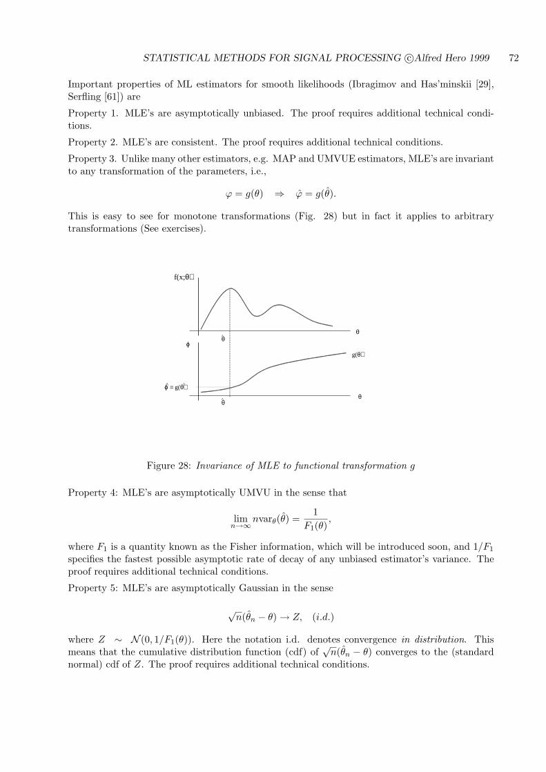
STATISTICAL METHODS FOR SIGNAL PROCESSING c©Alfred Hero 1999 72
Important properties of ML estimators for smooth likelihoods (Ibragimov and Has’minskii [29],Serfling [61]) are
Property 1. MLE’s are asymptotically unbiased. The proof requires additional technical condi-tions.
Property 2. MLE’s are consistent. The proof requires additional technical conditions.
Property 3. Unlike many other estimators, e.g. MAP and UMVUE estimators, MLE’s are invariantto any transformation of the parameters, i.e.,
ϕ = g(θ) ⇒ ϕ = g(θ).
This is easy to see for monotone transformations (Fig. 28) but in fact it applies to arbitrarytransformations (See exercises).
g(θ)
θ
θ
^
θ
^
^
ϕ
ϕ = g(θ)
θ
f(x;θ)
^
Figure 28: Invariance of MLE to functional transformation g
Property 4: MLE’s are asymptotically UMVU in the sense that
limn→∞nvarθ(θ) =
1F1(θ)
,
where F1 is a quantity known as the Fisher information, which will be introduced soon, and 1/F1
specifies the fastest possible asymptotic rate of decay of any unbiased estimator’s variance. Theproof requires additional technical conditions.
Property 5: MLE’s are asymptotically Gaussian in the sense
√n(θn − θ) → Z, (i.d.)
where Z ∼ N (0, 1/F1(θ)). Here the notation i.d. denotes convergence in distribution. Thismeans that the cumulative distribution function (cdf) of
√n(θn − θ) converges to the (standard
normal) cdf of Z. The proof requires additional technical conditions.
STATISTICAL METHODS FOR SIGNAL PROCESSING c©Alfred Hero 1999 73
Property 6: The MLE is equivalent to the MAP estimator for a uniform prior f(θ) = c.
Property 7: If the MLE is unique, the MLE is a function of the data only through the sufficientstatistic.
Now let’s go back and revisit our MOM examples with the MLE in mind.
Example 15 X i.i.d. Bernoulli random variables
We can solve for the MLE in two ways: (1) considering the entire observation X; and (2) consid-ering only a sufficient statistic T (X).
1. With the entire observation X = x the likelihood function is the product
L(θ) = f(x; θ) =n∏
i=1
θxi(1− θ)1−xi .
Is is convenient to rewrite this in the form
L(θ) = θPn
i=1 xi(1− θ)n−Pni=1 xi
= θnxi(1− θ)n−nxi . (31)
As this function smooth and concave in θ, differentiation with respect to θ yields a stationarypoint condition, the ”ML equation,” for the MLE θ
0 =∂
∂θf(x; θ) = n
[(1− θ)xi − θ(1− xi)
θ(1− θ)
]f(x; θ).
Solving the equation (1− θ)xi − θ(1− xi) = 0 we obtain the MLE
θ = X, (32)
which is identical to the MOM estimator obtained above.
2. Using the Fisher factorization (21) on the p.d.f. (31) of X it is easily seen that T (X) =∑ni=1 Xi is a sufficient statistic for θ. The distribution of T is binomial with parameter θ:
fT (t; θ) =(
n
t
)θt(1− θ)n−t, t = 0, . . . , n,
where the subscript T on the density of T is to clarify that this is the p.d.f. of the r.v. T .Identification of t = nX reveals that this is of exactly the same form, except for a constantmultiplication factor, as (31). The ML equation is therefore the same as before and we obtainthe identical MLE estimator (32).
Example 16 X i.i.d. Poisson random variables
To find the MLE of the rate parameter θ express the density of the samples as:
f(x; θ) =n∏
i=1
θxi
xi!e−θ.
STATISTICAL METHODS FOR SIGNAL PROCESSING c©Alfred Hero 1999 74
The likelihood function L(θ) = f(x; θ) has to be maximized over θ to produce the MLE. It is moreconvenient to deal with the log likelihood
θml = argmaxθ>0 ln L(θ)
and we have
l(θ) = ln f(x; θ)
= lnn∏
k=1
θxk
xk!e−θ
=n∑
k=1
xk ln θ − nθ −n∑
k=1
ln xk!
︸ ︷︷ ︸constant in θ
= xin ln θ − nθ + c,
where c is an irrelevant constant.
It is easily verified (look at second derivative) that the log-likelihood l(θ) is a smooth strictlyconcave function of θ. Thus the MLE is the unique solution θ = θ of the equation
0 = ∂ ln f/∂θ =nxi
θ− n.
We find that the MLE is identical to the first MOM estimator we found for this problem:
θ = X,
which we know is unbiased with variance equal to θ.
Let’s check the asymptotic Gaussian property. Write
√n(X − θ) =
√n
(1n
n∑
i=1
(Xi − θ)
)
=1√n
n∑
i=1
(Xi − θ).
By the central limit theorem (CLT), this converges in distribution to a Gaussian r.v.
Eθ[√
n(X − θ)] = 0varθ(
√n(X − θ)) = θ.
4.4.4 SCALAR CRAMER-RAO BOUND (CRB) ON ESTIMATOR VARIANCE
The CRB can be defined for both random and non-random parameters. However the CRB is moreuseful for non-random parameters as it can be used to establish optimality or near optimality ofan unbiased candidate estimator. Unlike the non-random case, for random parameters the optimalestimator and its MSE are functions of the known joint density of θ and X. Thus there exist moreaccurate alternatives to the CRB for approximating estimator MSE, most of which boil down toapproximating an integral representation of the minimum mean squared error. We therefore focus
STATISTICAL METHODS FOR SIGNAL PROCESSING c©Alfred Hero 1999 75
our energies on the CRB for non-random parameters - the interested reader can refer to [72] forthe random case.
Let θ ∈ Θ be a non-random scalar and assume:
1. Θ is an open subset, e.g. (a, b), of IR.
2. f(x; θ) is smooth (Ibragimov and Has’minskii [29]) and differentiable in θ.
The following is the Cramer-Rao bound for scalar θ
For any unbiased estimator θ of θ
varθ(θ) ≥ 1/F (θ), , (33)
where “=” is attained iff for some non-random scalar kθ
∂
∂θln f(x; θ) = kθ(θ − θ). (34)
Here kθ is a constant that can depend on θ but not on x. When the CRB is attainable it is saidto be a tight bound and (34) is called the CRB tightness condition.
In the CRB F (θ) is the Fisher information which can be shown [72] to take on either of thefollowing two equivalent forms:
F (θ) = Eθ
[(∂
∂θln f(X; θ)
)2]
= −Eθ
[∂2
∂θ2ln f(X; θ)
]
Before going on to some examples, we provide a simple derivation of the scalar CRB here. A moredetailed proof of the more general vector parameter CRB will be given later. There are three stepsto the derivation of the scalar CRB. The first step is to notice that the mean of the derivative ofthe log-likelihood is equal to zero:
Eθ[∂ ln fθ(X)/∂θ] = Eθ
[∂fθ(X)/∂θ
fθ(X)
]
=∫
∂
∂θfθ(x)dx
=∂
∂θ
∫fθ(x)
︸ ︷︷ ︸=1
dx
= 0
The second step is to show that the correlation between the derivative of the log-likelihood andthe estimator is a constant:
Eθ[(θ(X)− Eθ[θ])(∂logfθ(X)/∂θ)] =∫
(θ(x)−Eθ[θ])∂
∂θfθ(x)dx
=∂
∂θ
∫θ(x)fθ(x)
︸ ︷︷ ︸=Eθ[θ]=θ
dx
= 1
STATISTICAL METHODS FOR SIGNAL PROCESSING c©Alfred Hero 1999 76
Where we have used the result of step 1 in line 2 above. Finally, apply the Cauchy-Schwarz (CS)inequality E2[UV ] ≤ E[U2]E[V 2] to obtain:
1 = E2θ [(θ(X)−Eθ[θ])(∂ ln fθ(X)/∂θ)]
≤ Eθ[(θ(X)−Eθ[θ])2] · Eθ[(∂ ln fθ(X)/∂θ)2]= varθ(θ) · F (θ).
Equality occurs in the CS inequality if and only if U = kV for some non-random constant k. Thisgives (33) and completes the derivation of the CRB.
To illustrate the CRB let’s go back and reconsider one of the previous examples.
Example 17 CRB for the Poisson rate
Assume again that X = [X1, . . . , Xn] is a vector of i.i.d. Poisson random variables
Xi ∼ f(x; θ) =θx
x!e−θ, x = 0, 1, 2, . . .
To find the CRB we must first compute the Fisher information. Start with
ln f(x; θ) =n∑
k=1
xk ln θ − nθ −n∑
k=1
ln xk!
︸ ︷︷ ︸constant in θ
,
and differentiate twice
∂ ln f(x; θ)/∂θ =1θ
n∑
k=1
xk − n (35)
∂2 ln f(x; θ)/∂θ2 = − 1θ2
n∑
k=1
xk. (36)
Therefore, as E[∑n
k=1 Xk] = nθ, the Fisher information given the n i.i.d. samples is
Fn(θ) =n
θ.
The CRB asserts that for any unbiased estimator of the Poisson rate θ
varθ(θ) ≥ θ
n.
It is useful to make the following key observations.
Observation 1: From example (14) we know that the sample mean X is unbiased and has varθ(X) =θ/n. This is equal to the CRB and we conclude the CRB is tight.
Observation 2: In fact we could have concluded by inspection that the unbiased estimator Xachieves the CRB; i.e., without having to explicitly compute its variance and compare to one
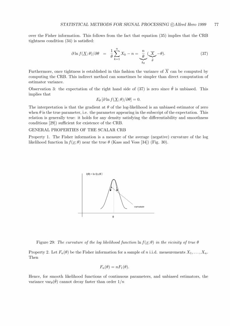
STATISTICAL METHODS FOR SIGNAL PROCESSING c©Alfred Hero 1999 77
over the Fisher information. This follows from the fact that equation (35) implies that the CRBtightness condition (34) is satisfied:
∂ ln f(X; θ)/∂θ =1θ
n∑
k=1
Xk − n =n
θ︸︷︷︸kθ
( X︸︷︷︸θ
−θ). (37)
Furthermore, once tightness is established in this fashion the variance of X can be computed bycomputing the CRB. This indirect method can sometimes be simpler than direct computation ofestimator variance.
Observation 3: the expectation of the right hand side of (37) is zero since θ is unbiased. Thisimplies that
Eθ [∂ ln f(X; θ)/∂θ] = 0.
The interpretation is that the gradient at θ of the log-likelihood is an unbiased estimator of zerowhen θ is the true parameter, i.e. the parameter appearing in the subscript of the expectation. Thisrelation is generally true: it holds for any density satisfying the differentiability and smoothnessconditions [29]) sufficient for existence of the CRB.
GENERAL PROPERTIES OF THE SCALAR CRB
Property 1. The Fisher information is a measure of the average (negative) curvature of the loglikelihood function ln f(x; θ) near the true θ (Kass and Voss [34]) (Fig. 30).
θ
l(θ) = ln f(x;θ)
curvature
Figure 29: The curvature of the log likelihood function ln f(x; θ) in the vicinity of true θ
Property 2. Let Fn(θ) be the Fisher information for a sample of n i.i.d. measurements X1, . . . , Xn.Then
Fn(θ) = nF1(θ).
Hence, for smooth likelihood functions of continuous parameters, and unbiased estimators, thevariance varθ(θ) cannot decay faster than order 1/n
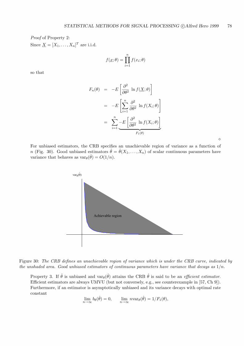
STATISTICAL METHODS FOR SIGNAL PROCESSING c©Alfred Hero 1999 78
Proof of Property 2:
Since X = [X1, . . . , Xn]T are i.i.d.
f(x; θ) =n∏
i=1
f(xi; θ)
so that
Fn(θ) = −E
[∂2
∂θ2ln f(X; θ)
]
= −E
[n∑
i=1
∂2
∂θ2ln f(Xi; θ)
]
=n∑
i=1
−E
[∂2
∂θ2ln f(Xi; θ)
]
︸ ︷︷ ︸F1(θ)
¦For unbiased estimators, the CRB specifies an unachievable region of variance as a function ofn (Fig. 30). Good unbiased estimators θ = θ(X1, . . . , Xn) of scalar continuous parameters havevariance that behaves as varθ(θ) = O(1/n).
var^
n
Achievable region
Figure 30: The CRB defines an unachievable region of variance which is under the CRB curve, indicated bythe unshaded area. Good unbiased estimators of continuous parameters have variance that decays as 1/n.
Property 3. If θ is unbiased and varθ(θ) attains the CRB θ is said to be an efficient estimator.Efficient estimators are always UMVU (but not conversely, e.g., see counterexample in [57, Ch 9]).Furthermore, if an estimator is asymptotically unbiased and its variance decays with optimal rateconstant
limn→∞ bθ(θ) = 0, lim
n→∞nvarθ(θ) = 1/F1(θ),
STATISTICAL METHODS FOR SIGNAL PROCESSING c©Alfred Hero 1999 79
then θ is said to be asymptotically efficient.
Property 4. Efficient estimators for θ can only exist when the underlying model is in an exponentialfamily, defined in Sec. 3.5.4:
f(x; θ) = a(θ)b(x)e−c(θ)t(x),
and when Eθ[t(X)] = θ, i.e., the density is in its natural parameterization (recall Sec. 3.5.4).Furthermore, when an i.i.d. sample X = [X1, . . . , Xn]T is available θ = n−1
∑ni=1 t(xi) is an
efficient estimator of θ.
Proof of Property 4:
Without loss of generality we specialize to the case of a single sample n = 1 and Θ = (−∞,∞).Recall the condition for equality in the CR bound to be achieved by an estimator θ is that thep.d.f. be expressible as
∂
∂θln f(x; θ) = kθ(θ − θ). (38)
For fixed θo, integrate the LHS of condition (38) over θ ∈ [θo, θ′]
∫ θ′
θo
∂
∂θln f(x; θ)dx = ln f(x; θ′)− ln f(x; θo).
On the other hand, integrating the RHS of the condition∫ θ′
θ0
kθ′(θ − θ) dθ =∫ θ′
θo
kθ(θ − θ)dθ
= θ
∫ θ′
θo
kθdθ
︸ ︷︷ ︸c(θ′)
−∫ θ′
θo
kθθdθ
︸ ︷︷ ︸d(θ′)
.
Or combining the integrals of RHS and LHS of (38)
f(x; θ) = e−d(θ)︸ ︷︷ ︸a(θ)
f(x; θo)︸ ︷︷ ︸b(x)
e−c(θ)
t(x)︷︸︸︷θ .
¦We illustrate the above with two more examples.
Example 18 Parameter estimation for the exponential density.
A non-negative random variable X has an exponential density with mean θ if its p.d.f. is of the formf(x; θ) = θ−1exp(−x/θ) where θ > 0. The exponential random variable is commonly used as amodel for service time or waiting time in networks and other queuing systems. You can easily verifythat this density is in the exponential family specified by a(θ) = θ−1, b(x) = I[0,∞)(x), c(θ) = −θ−1
and t(x) = x. Thus, as Eθ[t(X)] = θ, the p.d.f. f(x; θ) is in its natural parametrization and weconclude that the sample mean X is an efficient, and therefore UMVU, estimator of θ when n i.i.d.observations X = [X1, . . . , Xn]T are available.
NOTE: we cannot conclude that 1/X is an efficient (or even an unbiased) estimator of 1/θ. Infact it is even worse than this: we cannot conclude that a UMVUE exists for 1/θ since the changeof parameter to α = 1/θ destroys the natural parameterization of the density.

STATISTICAL METHODS FOR SIGNAL PROCESSING c©Alfred Hero 1999 80
Example 19 X i.i.d., Xi ∼ N (θ, σ2)
The Gaussian ”bell curve” distribution arises in so many applications that it has become a standardmodel. Use of this model is usually justified by invocation of the Central Limit Theorem asdescribing the measurements, or measurement noise, as the sum of many small contributions, e.g.random atomic collisions, scattered light, aggregation of repeated measurements.
Our first objective will be to find the MLE and CRB for estimating the mean θ of univariateGaussian with known variance σ2. As the Gaussian with unknown mean is in the exponentialfamily we could take the same approach as above to find efficient estimators. But let’s spice thingsup and follow an alternative route of trying to tease an efficient estimator out of the tightnesscondition in the CRB.
f(x; θ) =(
1√2πσ2
)n
exp
− 1
2σ2
n∑
k=1
(xk − θ)2
.
Or
ln f(x; θ) = −n
2ln(σ2)− 1
2σ2
n∑
k=1
(xk − θ)2 + c,
where c is constant. Compute the first derivative
∂ ln f/∂θ =1σ2
n∑
k=1
(xk − θ)
=n
σ2︸︷︷︸kθ
(xi − θ). (39)
Thus the CRB tightness condition (34) is satisfied and we can identify, once again, the samplemean xi as the optimal estimator of the common mean of a Gaussian sample.
We take another derivative of the log-likelihood with respect to θ and invert it to verify what wealready knew about the variance of the sample mean
varθ(X) = 1/Fn(θ) = σ2/n.
The first inequality is only true since we know that X is efficient.
Note that the leading factor in the tight CRB condition (39) is: kθ = var−1θ (X). This is always
true for efficient estimators when kθ does not depend on θ.
4.5 ESTIMATION OF MULTIPLE NON-RANDOM PARAMETERS
We now turn the more general problem of many unknown deterministic parameters. This problemis quite different from the previously studied case of multiple random parameters since there is nojoint posterior density to marginalize. First we arrange all unknown parameters in a vector:
θ = [θ1, . . . , θp]T ,
and state the problem as finding a vector valued estimator θ of θ.
STATISTICAL METHODS FOR SIGNAL PROCESSING c©Alfred Hero 1999 81
The joint density for the measurements X is written as:
f(x; θ1, . . . , θp) = f(x; θ).
POSSIBLE ESTIMATOR PERFORMANCE CRITERIA
As for a scalar estimator we define the vector estimator bias vector:
bθ(θ) = Eθ[θ]− θ,
and the symmetric estimator covariance matrix:
covθ(θ) = Eθ[(θ − E[θ])(θ −E[θ])T ]
=
varθ(θ1) covθ(θ1, θ2) . . . covθ(θ1, θp)
covθ(θ2, θ1) varθ(θ2). . .
......
. . . . . ....
covθ(θp, θ1) · · · · · · varθ(θp)
.
This matrix is often referred to as the variance-covariance matrix.
In many cases, only the diagonal entries of the estimator covariance matrix, i.e. the componentestimator variances, will be of interest. However, as we will soon see, the entire estimator covariancematrix is very useful for generalizing the scalar parameter CRB.
We can also define the estimator concentration:
Pθ(‖θ − θ‖ > ε) =∫
‖θ−θ‖>εf(θ; θ)dθ
=∫
x:‖θ(x)−θ‖>εf(x; θ)dx
The first order of business is to extend the CRB to vector parameters, called the matrix CRB.
4.5.1 MATRIX CRAMER-RAO BOUND (CRB) ON COVARIANCE MATRIX
Let θ ∈ Θ be a p× 1 vector and assume:
1. Θ is an open subset of IRp
2. f(x; θ) is smooth [29] and differentiable in θ
3. covθ(θ) and F(θ) (defined below) are non-singular matrices
The matrix CRB for vector valued parameters is the following. For any unbiased estimator θ of θ
covθ(θ) ≥ F−1(θ), (40)
where “=” is attained iff the following is satisfied for some non-random matrix Kθ
Kθ∇θ ln f(X; θ) = θ − θ. (41)
In the case that this tightness condition (41) is satisfied θ is said to be an efficient vector estimator.
STATISTICAL METHODS FOR SIGNAL PROCESSING c©Alfred Hero 1999 82
In the matrix CRB (40) F(θ) is the Fisher information matrix, which takes either of two equivalentforms,
F(θ) = E[(∇θ ln f(X; θ)
) (∇θ ln f(X; θ))T
]
= −E[∇2
θ ln f(X; θ)].
where we have defined the gradient operator
∇θ =[
∂
∂θ1, . . . ,
∂
∂θp
]T
,
and the symmetric Hessian (curvature) operator
∇2θ =
∂2
∂θ21
∂2
∂θ1∂θ2. . . ∂2
∂θ1∂θp
∂2
∂θ2∂θ1
∂2
∂θ22
. . ....
.... . . . . .
...∂2
∂θp∂θ1· · · · · · ∂2
∂θ2p
.
The matrix CR Bound (40) has a few more properties than the scaler CRB.
Property 1: The inequality in the matrix bound should be interpreted in the sense of positivedefiniteness. Specifically if A,B are p× p matrices
A ≥ B ⇐⇒ A−B ≥ 0,
where A−B ≥ 0 means A−B is non-negative definite. This means that, in particular,
zT (A−B)z ≥ 0
for any vector z ∈ IRp, and all eigenvalues of A − B are non-negative. For example, choosingz = [1, 0, . . . , 0]T : and z = [1, . . . , 1]T , respectively, A ≥ B, A ≥ B implies both
aii ≥ bii, and∑
i,j
aij ≥∑
ij
bij .
However, A ≥ B does NOT mean aij ≥ bij in general. A simple counterexample is constructed asfollows. Let 0 < ρ < 1 and consider
[2 00 2
]
︸ ︷︷ ︸A
−[
1 ρρ 1
]
︸ ︷︷ ︸B
=[
1 −ρ−ρ 1
],
which has two eigenvalues 1− ρ > 0 and 1 + ρ > 0. Hence A−B > 0 while clearly a12 = 0 6> ρ.
Property 2: The matrix inequality (40) implies a scalar CRB on the variance of the i-th componentof an unbiased vector estimator θ
varθ(θi) ≥ [F−1(θ)]ii,
where the right hand side (RHS) denotes the i-th element along the diagonal of the inverse Fisherinformation matrix.
STATISTICAL METHODS FOR SIGNAL PROCESSING c©Alfred Hero 1999 83
Property 3. Fisher information matrix is a measure of the average curvature profile of the loglikelihood near θ
Property 4. Let Fn(θ) be the Fisher information for a sample of n i.i.d. measurements X1, . . . , Xn.Then, as in the scalar parameter case,
Fn(θ) = nF1(θ).
Hence varθ(θ) = O(1/n) is also expected for good estimators of multiple unknown continuousvalued parameters.
Property 5. Efficient vector estimators only exist for multiparameter exponential families
f(x; θ) = a(θ)b(x)e−[c(θ)]T [t(x)]
When f(x; θ) is in its natural parameterization and E[n−1∑n
i=1 t(Xi)] = θ, θ = n−1∑n
i=1 t(Xi) isan unbiased efficient estimator.
Property 6. If an estimator θ satisfies
∇θ ln f = Kθ(θ − θ),
then we can immediately conclude:
1. θ is unbiased since, as shown in proof of the multiple parameter CRB;
Eθ[∇θ ln f(X; θ)] = 0,
2. θ is efficient and thus its components are UMVU estimators;
3. The covariance of θ is given by the inverse Fisher information F(θ);
4. If Kθ = K (not a function of θ) then F(θ) = K and
covθ(θ) = K−1.
Proof of Matrix CR bound:
There are 3 steps in our derivation, which, with one exception, is a direct generalization of theproof of the scalar CRB: (1) show that the gradient of the log-likelihood is zero mean; (2) thecorrelation between the gradient of the log-likelihood and estimator is constant; (3) the covariancematrix of the concatenated gradient and estimator error gives a relation between Fisher info andestimator covariance.
Step 1. Show Eθ
[∇θ ln f(X; θ)]
= 0.
⇒ = Eθ
[1
f(X; θ)∇θf(X; θ)
]=
∫
X∇θf(x; θ)dx
= ∇θ
∫
Xf(x; θ)dx
︸ ︷︷ ︸=1
= 0.
Step 2. Eθ
[∇θ ln f(X; θ) (θ − θ)T
]= I.

STATISTICAL METHODS FOR SIGNAL PROCESSING c©Alfred Hero 1999 84
First observe
Eθ
[∇θ ln f(X; θ) θ
T]
= Eθ
[1
f(X; θ)∇θf(X; θ)θ
T]
=∫
X∇θf(x; θ)θ
T(x)dx
= ∇θ
∫
Xf(x; θ)θ
T(x)dx
︸ ︷︷ ︸Eθ[θ
T]=θT
= I.
Now putting this together with result of the previous step
Eθ
[∇θ ln f(X; θ) (θ − θ)T
]
= Eθ
[∇θ ln f(X; θ) θ
T]
︸ ︷︷ ︸=I
−Eθ
[∇θ ln f(X; θ)]
︸ ︷︷ ︸=0
θT .
Step 3. Define a 2p× 1 random vector U :
U =[
θ − θ∇θ ln f(X; θ)
]. (42)
Since any matrix expressed as an outer product of two vectors is non-negative definite
Eθ
[UUT
] ≥ 0.
Using the results of steps 1 and 2, we have
Eθ
[UUT
]=
[covθ(θ) I
I F(θ)
]≥ 0.
It only remains to apply the result of Sec. 2.4 to the above partitioned matrix to see that thisimplies that
covθ(θ)− F−1(θ) ≥ 0.
An alternative, and more direct, way to show this is to let w and y be arbitrary p-vectors and
define v =[
wy
]. Then, as vT Eθ
[UUT
]v ≥ 0,
wT covθ(θ)w + 2wT y + yTF(θ)y ≥ 0.
Taking y = −F−1(θ) w in the above we obtain
wT [covθ(θ)− F−1(θ)]w ≥ 0.
It remains to obtain the tightness condition ensuring equality in the CRB. Note first that ifcovθ(θ) = F−1 then Eθ[UUT ] necessarily has rank p (see exercises at end of chapter). This can

STATISTICAL METHODS FOR SIGNAL PROCESSING c©Alfred Hero 1999 85
only happen if the random vector U (42) has p linearly independent components. As covθ(θ) andF(θ) have been assumed non-singular, θ − θ can have no linear dependencies and neither does∇θ ln f . Hence it can only be that
Kθ∇θ ln f = θ − θ
for some non-random matrix Kθ. In other words the gradient of the log likelihood lies in the spanof the estimator errors. ¦We move on to generalizations of MOM and ML estimators to the vector parameter case.
4.5.2 METHODS OF MOMENTS (MOM) VECTOR ESTIMATION
Let mk = mk(θ) be the k-th order moment of f(x; θ). The vector MOM estimation procedureinvolves finding K moments such that the vector function of θ ∈ IRp
g(θ) = [m1(θ), . . . , mK(θ)]
can be inverted, i.e., there exists a unique value θ satisfying
θ = g−1(m1, . . . ,mK).
As in the scalar case, the MOM estimator is constructed by replacing mk with its empirical estimate
θ = g−1(m1, . . . , mK),
where mk = 1n
∑ni=1 Xk
i .
4.5.3 MAXIMUM LIKELIHOOD (ML) VECTOR ESTIMATION
The vector MLE is an obvious generalization of the scalar MLE
θ = argmaxθ∈Θf(X; θ).
For smooth likelihood functions, vector MLEs have several key properties ([29]):
1. Vector MLE’s are asymptotically unbiased;
2. Vector MLE’s are consistent;
3. Vector MLE’s are invariant to arbitrary vector transformations;
ϕ = g(θ) ⇒ ϕ = g(θ);
4: Vector MLE’s are asymptotically efficient and thus their component estimators are asymptoti-cally UMVU;
5. Vector MLE’s are asymptotically Gaussian in the sense√
n(θn − θ) → z, (i.d.)
where z ∼ Np(0,F−11 (θ)) and F1(θ) is the single sample Fisher information matrix
F1(θ) = −Eθ
[∇2
θ log f(X1; θ)].
A couple of examples will illustrate these estimators.
STATISTICAL METHODS FOR SIGNAL PROCESSING c©Alfred Hero 1999 86
Example 20 Joint estimation of mean and variance in a Gaussian sample
This is an extension of Example 20 to the case where both the mean and the variance are unknown.Assume an i.i.d. sample X = [X1, . . . , Xn] of Gaussian r.v.s Xi ∼ N (µ, σ2). The unknowns areθ = [µ, σ2].
The log-likelihood function is
l(θ) = ln f(x; θ) = −n
2ln(σ2)− 1
2σ2
n∑
k=1
(xk − µ)2 + c. (43)
A. MOM approach to estimation:
We know that m1 = µ, m2 = σ2 + µ2 and thus
µ = m1, σ2 = m2 −m21.
Hence a MOM estimator of θ is:
θ = [µ, σ2]= [m1, m2 − m2
1]
=[X, X2 −X
2]
=[X, (X −X)2
].
As usual we denote
X = n−1n∑
k=1
Xk
(X −X)2 = n−1n∑
k=1
(Xk −X)2 =n− 1
ns2,
and
s2 = (n− 1)−1n∑
k=1
(Xk −X)2
is the sample variance.
B. ML approach.
As l(θ) (43) is a concave function (verify that −∇2θ ln f is positive definite) we can use the likelihood
equation (stationary point condition) for finding θ = θ
0 = ∇θ ln f(x; θ) =
1θ2
∑nk=1(xk − θ1)
n/2θ2− 1
2θ22
∑nk=1(xk − θ1)2
.
Therefore,
θ1 = µ = X, θ2 = σ2 =n− 1
ns2,
STATISTICAL METHODS FOR SIGNAL PROCESSING c©Alfred Hero 1999 87
so that the MLE and MOM estimators are identical.
Let’s consider the performance of the ML/MOM estimator. The bias and covariance are simpleenough to compute (recall that in Sec. 3.4 we showed that (n− 1)s2/σ2 is Chi square distributedwith n− 1 degrees of freedom):
Eθ[µ] = µ︸ ︷︷ ︸unbiased
, Eθ[σ2] =(
n− 1n
)σ2
︸ ︷︷ ︸biased
;
varθ(X) = σ2/n;
and
varθ(σ2) =(
n− 1n
)2
varθ(s2) = 2σ4/n
(n− 1
n
).
Since the sample mean and sample variance are uncorrelated (recall Sec. 3.4)
covθ(θ) =[
σ2/n 00 2σ4/n
(n−1
n
)]
. (44)
Next we compute the Fisher information matrix by taking the expectation of the Hessian−∇2θ ln f(X; θ)
F(θ) =[
n/σ2 00 n/(2σ4)
], (45)
giving the CR bound
covθ(θ) ≥[
σ2/n 00 2σ4/n
]. (46)
Some interesting observations are the following:
Observation 1. MOM and ML estimators derived above have covariances which violate the CRbound (compare the (2,2) elements of matrices (44) and the RHS of (46)). This is not a contra-diction since the ML variance estimator is not unbiased!
Observation 2. Consider the bias-corrected estimator of [µ, σ2]T
ˆθ = [X, s2]T .
This estimator is unbiased. Now, as s2 =(
nn−1
)σ2
varθ(s2) =(
n
n− 1
)2
varθ(σ2),
covθ(ˆθ) =
[σ2/n 0
0 2σ4/n(
nn−1
)]≥ F−1(θ).
We conclude that the bias-corrected estimator’s covariance no longer violates the CRB. Indeed,X is efficient estimator of µ since
varθ(µ) = [F−1]11 = σ2/n.
STATISTICAL METHODS FOR SIGNAL PROCESSING c©Alfred Hero 1999 88
However, s2 is not an efficient estimator of σ2 since
varθ(s2) > [F−1]22.
Observation 3. as predicted, the MLE is asymptotically efficient as n →∞.
ncovθ(θ) =[
σ2 00 2σ4
(n−1
n
)]→
[σ2 00 2σ4
]= F−1
1 (θ).
Observation 4. We can also verify that, as predicted, [µ, σ2] is asymptotically Gaussian. It sufficesto consider the following results:
a) µ and σ2 are independent r.v.s;
b)√
n(µ− µ) = N (0, σ2);
c)√
n(s2 − σ2) = σ2√n(χ2n−1/(n− 1)− 1);
d) χ2ν ∼ N (ν, 2ν), ν →∞.
Observation 5. We can easily manipulate the condition for equality in the CR bound to find anefficient vector estimator (but not of θ as originally specified!):
∇θ ln f(X; θ) = Kθ
[X − µ
X2 − (σ2 + µ2)
],
where
Kθ :=[
n/σ2 00 n/2σ4
] [1 02µ 1
]−1
.
As the sample moments are unbiased estimates of the ensemble moments, we conclude that X, X2
are efficient estimators of the first moment E[X] = µ and second (non-central) moment E[X2] =σ2 + µ2, respectively.
We continue with another example, which requires special treatment due to functional dependen-cies that exist between parameters.
Example 21 N = [N1, . . . , Np]T a multinomial random vector
The multinomial model is a generalization of the binomial model to more than two categories, ”0”and ”1”, of outcome. Let the outcome Z of a single trial be one of the p elementary vectors in IRp,e1 = [1, 0, . . . , 0]T , . . . , ep = [0, 0, . . . , 1]T , with probabilities θ1, . . . , θp, respectively. The vector ek
could be a tag attached to the event that a random throw of a die resulted in a face with k dots(p = 6) or that a symbol received by a teletype (who remembers those?) corresponds to the k-thletter of the alphabet (p = 27). The multinomial model describes the distribution of the sum
N = [N1, . . . , Np]T =n∑
i=1
Zi
of these vectors obtained after n i.i.d. trials.
The probability of a particular multinomial outcome N gives the probability mass function
p(N ; θ) =n!
N1! · · · Np!θN11 . . . θ
Npp .
STATISTICAL METHODS FOR SIGNAL PROCESSING c©Alfred Hero 1999 89
where Ni ≥ 0 are integers satisfying∑p
i=1 Ni = n and θi ∈ [0, 1] are cell probabilities satisfying∑pi=1 θi = 1.
A MOM estimator of θ is obtained by matching the first empirical moment N to the first ensemblemoment Eθ[N ] = θn. This yields the estimator θ = N/n, or more explicitly
θ =[N1
n, . . . ,
Np
n
]
To find the MLE of θ we need to proceed with caution. The p parameters θ live in a p−1 subspaceof IRp due to total cell probability constraint. We can find the MLE either by reparameterizationof the problem or by using Lagrange multipliers. The Lagrange multiplier method will be adoptedhere.
To account for the constraint we replace the log-likelihood function with the penalized log-likelihood function
J(θ) = ln f(N ; θ)− λ
(p∑
i=1
θi − 1
),
where λ is a Lagrange multiplier which will be selected. in order to satisfy the constraint.
Now as J is smooth and concave we set the gradient of J(θ) to zero to find the MLE:
0 = ∇θJ(θ) = ∇θ
[p∑
i=1
Ni ln θi − λθi
]
=[N1
θ1− λ, . . . ,
Np
θp− λ
].
Thusθi = Ni/λ, i = 1, . . . , p
Finally, we find λ by forcing θ to satisfy constraint
p∑
i=1
Ni/λ = 1 ⇒ λ =p∑
i=1
Ni = n.
The solution to this equation gives the MLE and it is identical to the MOM estimator.
To derive the CRB requires more advanced theory of constrained CR bounds [20] since the θi’sare linearly dependent.
4.6 HANDLING NUISANCE PARAMETERS
In many cases only a single parameter θ1 is of direct interest while the other unknowns θ2, . . . , θp
are nuisance parameters which are not of interest. For example, in the Gaussian example withboth unknown mean and variance, Example 20, the variance may not be of intrinsic interest. Inthis example, we found that the estimator covariance is diagonal, which implies that there is nocorrelation between the mean parameter estimation errors and the variance parameter estimationerrors. As we will see below, this is means that the variance is a rather benign nuisance parametersince knowledge or lack of knowledge of the variance does not affect the variance of the MLmean estimator. We divide the discussion of nuisance parameters into the cases of random andnon-random parameters.
STATISTICAL METHODS FOR SIGNAL PROCESSING c©Alfred Hero 1999 90
CASE I: HANDLING RANDOM NUISANCE PARAMETERS:
For random parameters the average cost only penalizes θ1’s estimation errors:
E[c(θ1, θ1)] =∫
Θ1
dθ1
∫
Xdx c(θ1(x), θ1)f(x|θ1)f(θ1).
The prior on θ1 is computed from the prior on θ
f(θ1) =∫
dθ2 . . .
∫dθp f(θ1, θ2, . . . , θp).
The conditional density of X given θ1 is therefore
f(x|θ1) =∫
dθ2 . . .
∫dθp f(x|θ1, θ2, . . . , θp)f(θ2, . . . , θp|θ1),
yielding the posterior on θ1
f(θ1|x) =∫
dθ2 . . .
∫dθp f(θ1, . . . , θp|x).
Observe that explicit estimates of θ2, . . . , θp are not required to implement the posterior distri-bution of θ1. However, integration (marginalization) of the conditional density over θ2, . . . , θp isrequired and this may be quite difficult.
CASE II: HANDLING NON-RANDOM NUISANCE PARAMETERS:
The case of non-random parameters is quite different. The average cost still only penalizes for θ1
estimation errors but nonetheless depends on all unknowns:
Eθ[C] =∫
Xc(θ1(x), θ1)f(x; θ) dx.
The maximum Likelihood Estimator of θ1 is simply
θ1 = argmaxθ1
(max
θ2,...,θp
log f(X|θ1, θ2, . . . , θp))
.
Note that now we require maximization over all nuisance parameters or, equivalently, explicitestimates of the nuisance parameters are necessary.
CR BOUND PREDICTIONS FOR NON-RANDOM NUISANCE PARAMETERS
As above let’s say we are interested in unbiased estimation of only the first entry θ1 in the vectorof unknown parameters θ. Our derivation of the matrix CRB (40) made the explicit assumptionthat there existed unbiased estimators of all of the parameters. It turns out that this restrictionis unnecessary when only θ1 is of interest (see exercises).
Assume that θ = [θ1, . . . , θp]T is an unknown parameter vector. The variance of any unbiasedestimator θ1 of θ1 obeys the lower bound:
varθ(θ) ≥ [[F−1(θ)]]11, (47)
where equality occurs iff there exists a nonrandom vector hθ such that
hTθ ∇θ ln f(X; θ) = (θ1 − θ1).
STATISTICAL METHODS FOR SIGNAL PROCESSING c©Alfred Hero 1999 91
In (47) [[A]]ij denotes the ij entry of matrix A, and as before
F(θ) = −E
∂2l(θ)∂θ2
1
∂2l(θ)∂θ1∂θ2
. . . ∂2l(θ)∂θ1∂θp
∂2l(θ)∂θ2∂θ1
∂2l(θ)∂θ2
2
. . ....
.... . . . . .
...∂2l(θ)∂θp∂θ1
· · · · · · ∂2l(θ)∂θ2
p
,
and l(θ) = ln f(x; θ).
Let the Fisher matrix be partitioned as
F(θ) =[
a bT
b C
],
where
* a = −Eθ[∂2 ln f(X; θ)/∂θ21] = Fisher info for θ1 without nuisance parameters,
* b = −Eθ[∂∇θ2,...,θp ln f(X; θ)/∂θ1] = Fisher coupling of θ1 to nuisance parameters,
* C = −Eθ[∇2θ2,...,θp
ln f(X; θ)] = Fisher info for nuisance parameters.
Using the partitioned matrix inverse identity (2) the RHS of CRB (47) can be expressed as
[[F−1(θ)]]11 =1
a− bTC−1b.
This gives several insights:
Observation 1: [[F−1(θ)]]11 ≥ 1/a = 1/[[F(θ)]]11. Thus presence of nuisance parameters can onlydegrade estimator performance;
Observation 2: the amount of degradation is directly proportional to the amount of informationcoupling between θ1 and θ2, . . . , θp;
Observation 3: no degradation occurs when the Fisher matrix is block diagonal;
4.7 BACKGROUND REFERENCES
One of my favorite introductory texts covering estimation theory is the book on mathematicalstatistics by Mood, Graybill and Boes [47], mentioned before, which is concise, easy to read,and has many interesting examples and exercises. Nice books on this subject that focus on theBayesian point of view are Ferguson and [16] and DeGroot [14]. A good survey of Bayesian toolsfor statistical inference, and estimation in particular, is the book by Tanner [70]. Texts whichhave more of an engineering flavor are the now classic book by Van Trees [72], and the morerecent books by Kay [36], Srinath, Rajasekaran and Viswanathan [66], and Scharf [59]. For a moreadvanced treatment, requiring some background in real analysis, I like Bickel and Doksum [7],Lehmann [39], and Ibragimov and Has’minskii [29], and Poor [54].
STATISTICAL METHODS FOR SIGNAL PROCESSING c©Alfred Hero 1999 92
4.8 EXERCISES
4.1 Prove the formula |a + ∆| = |a|+ sgn(a)∆ + [sgn(a + ∆)− sgn(a)](a + ∆) in Sec. 4.2.2.4.2 Show the equivalence of the two expressions (24) and (25).4.3 Let X = [X1, . . . , Xn]T be a vector of i.i.d. r.v.s Xi which are uniformly distributed over the
interval (θ1, θ2), θ1 < θ2. Find the maximum likelihood estimator of θ.4.4 Let Zi, i = 1, . . . , n, be a set of i.i.d. random variables each with the alpha density
pθ(z) =β√
2πΦ(α)z2exp
(− 1
2 [α− β/z]2)
,
where β > 0 is unknown, α is known and Φ(x) =∫ x−∞
1√2π
e−u2/2du is the standard normal
CDF. Assuming that α = 0 and that β has an exponential prior density: p(β) = 1σβ
e−β/σβ ,where σβ > 0 is known. Find an expression for the MAP estimate of β. What does the MAPestimate reduce to as σβ →∞ (least informative prior)?
4.5 Let Wi, i = 1, . . . , n, be a set of zero mean i.i.d. Gaussian random variables with varianceσ2
w. Let a be a zero mean Gaussian random variable with variance σ2a which is independent
of Wi. The objective is to estimate the value of a given the observation
Xi = a + Wi, i = 1, . . . , n
(a) Find the MMSE estimator of a. How does this estimator compare to the MAP andMMAE estimators of a?
(b) Compute the MSE of the MMSE estimator (Hint: express error as a sum of two in-dependent r.v.’s to simplify algebra). What happens to the MSE as n → ∞ or asSNR = σ2
a/σ2w →∞?
4.6 Let X = [X1, . . . , Xn]T be a vector of i.i.d. Gaussian r.v.s with mean µ and variance σ2 = µ2
(Xi ∼ N (µ, µ2)).(a) Find a method of moments (MOM) estimator of µ based on the first moment.(b) Find the maximum likelihood estimate of µ.
4.7 Let Xi, i = 1, . . . , n, be an i.i.d. sample from the shifted exponential density f(x; θ) = e−(x−θ),x ≥ θ, where θ is an unknown parameter −∞ < θ < ∞. Assume that n > 1.(a) Find a MOM estimator of θ.(b) Find the ML estimator of θ.(c) Assuming the exponential prior for θ, f(θ) = e−θ, θ ≥ 0, find the MAP estimator, the
MMSE estimator, and the MMAE estimator of θ given the i.i.d. sample (be careful withyour limits of integration in computing f(θ|x)!). What happens to these estimators asn →∞?
(d) Calculate the MSE of each of the estimators derived in part (c) (assume large n). Verifythat the MMSE estimator has the lowest MSE.
4.8 The mean square error of a certain unbiased estimator θ(x) of the mean of a measured randomvariable is equal to σ2/2 where σ2 = var(x). What if anything does this tell you about thedistribution of x (Hint: what does the CR bound say about distributions that are impossible)?
4.9 Available are n i.i.d. samples of a random variable X with density
f(x; θ) = 12
1 + 3θx2
1 + θ
where −1 ≤ x ≤ 1 and θ ≥ 0.
STATISTICAL METHODS FOR SIGNAL PROCESSING c©Alfred Hero 1999 93
(a) Is this density in the exponential family?(b) Is the sample mean a sufficient statistic? If so, prove it for general n. If not, give a
counterexample, e.g. specialize to n = 2.(c) Find a MOM estimator of θ.(d) Find the CR bound on estimator variance for any unbiased estimator of θ.(e) Using either numerical integration (MATLAB) or analysis find the bias and variance of
the MOM estimator and compare to the CR bound for large n (e.g. n = 100).
4.10 Let the observation X have conditionally uniform density
f(x|θ) =
1θ , 0 < x ≤ θ0, o.w.
where θ is a random variable with density
fθ(θ) =
θ exp(−θ), θ ≥ 00, o.w.
A useful formula (v ≥ 0):∫∞v ue−udu = (v + 1)e−v
(a) Find the MAP estimator of θ.(b) Find the minimum mean squared error estimator of θ.(c) Find the minimum mean absolute error estimator of θ.
4.11 Let Z be a single observation having density function
pθ(z) = (2θz + 1− θ), 0 ≤ z ≤ 1
where −1 ≤ θ ≤ 1.
(a) Assuming that θ is a nonrandom parameter, find and plot the maximum likelihood esti-mator of θ as a function of Z.
(b) Is the ML estimator unbiased? If so does it achieve the CR bound?(c) Now assume that θ is a random variable with uniform prior density: pθ(θ) = 1
2 , θ ∈[−1, 1]. Find and plot the minimum mean square error estimator of θ as a function of Z.
(d) Compute the conditional bias E[θ|θ]−θ and the conditional MSE E[(θ−θ)2|θ] given θ foreach of the estimators of part a and c. Plot the two conditional MSE functions obtainedand compare the MSE’s of the two estimators. Does one estimator perform uniformlybetter than the other?
4.12 X = [X1, . . . , Xn]T is an i.i.d. observation from the Gamma density
Xi ∼ f(x|θ) =1
Γ(θ)xθ−1e−x, x ≥ 0
where θ is an unknown non-negative parameter and Γ(θ) is the Gamma function. You shouldnote the useful formulii
Γ(θ) =∫ ∞
0xθ−1e−xdx and
Γ(θ + k)Γ(θ)
= θ(θ + 1) . . . (θ + k − 1)
.
(a) Find the CR bound on unbiased estimators of θ.
STATISTICAL METHODS FOR SIGNAL PROCESSING c©Alfred Hero 1999 94
(b) Find the first order MOM estimator of θ by matching ensemble mean to sample mean.Is your estimator unbiased? Compute the variance of your estimator.
4.13 In this exercise you will establish that UMVUE’s do not always exist. Let Z be a r.v. withprobability mass function
pθ(z) =
θ, z = −1(1− θ)2θz, z = 0, 1, 2, . . .
where θ ∈ (0, 1).
(a) Define the estimator
θo(z) =
1, z = −10, z = 0, 1, 2, . . .
.
Show that θo is an unbiased estimator of θ.(b) Note that any unbiased estimator θ can be expressed in the form θ = θo + U where
U = U(Z) is a statistic satisfying Eθ[U ] = 0 (any U satisfying this condition is calledan ancillary statistic). Using this condition and the form for the pmf of Z given above,establish that U must be of the form U(Z) = aZ for some non-random constant a (Hint:Z-transform tables may be helpful).
(c) Now find an expression for the variance of an unbiased θ and show that the value a whichminimizes the variance is a function of θ. Hence no single unbiased estimator can achieveminimum variance for all θ ∈ (0, 1) and therefore no UMVUE for θ exists.
(d) Show that a UMVUE for φ = (1− θ)2 does exist even though a UMVUE for θ does notexist (Hint: define φo(z) = 1 for z = 0 and φo(z) = 0, otherwise and repeat the steps inpart a through c).
4.14 The observation consists of x1, . . . , xn i.i.d. samples where xi ∼ f(x|θ) and
f(x|θ) =
1θx
1θ−1, 0 ≤ x ≤ 1
0, o.w.
where θ, 0 < θ < ∞ is an unknown parameter.
(a) Compute the CR bound on unbiased estimators of θ. Is there an estimator that achievesthe bound?
(b) Find the maximum likelihood estimator of θ.(c) Compute the mean and variance of the maximum likelihood estimator. Specify a function
ϕ = g(θ) for which the maximum likelihood estimator of ϕ is efficient.(d) From one of your answers to parts a-c you should be able to derive the following formula
∫ 1
0uβ ln
(1u
)du =
1(1 + β)2
, β > −1.
4.15 The measurement x = [x1, . . . , xn]T is i.i.d. Gaussian with unknown mean µ and varianceσ2.
(a) Show that the sample mean xi = n−1∑n
i=1 xi and sample variance s2 = (n−1)−1∑n
k=1(xk−xi)2 are unbiased estimators and that they are uncorrelated and independent random vari-ables (Hint: show that the Gaussian random variables xi − xi and xi are uncorrelatedfor i = 1, . . . , n).
STATISTICAL METHODS FOR SIGNAL PROCESSING c©Alfred Hero 1999 95
(b) Using the results of part (a) derive the covariance matrix for the estimator θ = [xi, s2]T .
(Hint: to save yourself lots of algebra you should represent s2 = s2(x) in terms of σ2
and the sample variance s2(z) for z a vector of n i.i.d. zero mean unit variance Gaussianvariables. Then use the representation (ch. 3 of course notes) s2(z) = 1
n−1 χn−1 andproperties of the Chi square r.v. to find the expression for variance of s2).
(c) Derive the CR bound on the covariance matrix of any unbiased estimator θ of θ =[θ1, θ2]T = [µ, σ2]T . Compare to the result of part (b).
4.16 Show that if the CR bound is attained with equality then Eθ[UUT ] has rank p, where U isgiven by (42). (Hint: show that the matrix
Eθ
[UUT
]=
[F−1(θ) I
I F(θ)
]
has rank p.)4.17 An alternative approach to parameter estimation is called the ”quantile matching method”
and you will explore this method here. Let f(x; θ) be a density of the continuous r.v. X pa-rameterized by the scalar parameter θ and define the theoretical cdf F (x; θ) =
∫ x−∞ f(u; θ)du.
For n i.i.d. realizations Xini=1 from f(x; θ) define the empirical cdf as the fraction of Xi’s
which are less than or equal to x:
F (x) =1n
n∑
i=1
I(−∞,x](Xi)
where IA(y) equals 1 if y ∈ A and zero otherwise (the indicator function of set A).(a) Derive the mean Eθ[F (x)] and covariance covθ(F (x), F (y)) of F . Show that F (x) is an
asymptotically consistent estimator of F (x; θ).(b) The quantile matching estimate (QME) θ is defined as that value of t which minimizes
∫ ∞
−∞|F (x; t)− F (x)|2dx (48)
Let θ be a location parameter: f(x; θ) = f(x − θ). Using the definition (48), show thatθ must satisfy the following equation (Hint: use integration by parts):
∫ ∞
−∞f(x− θ)F (x)dx− 1/2 = 0. (49)
Show that if θ is the unique solution to (49) it is an asymptotically consistent estimatorof θ (Hint: for θ = t fixed and non-random, compute mean square value of left hand sideof (49) and show that as n →∞ it goes to a function of t which equals zero at t = θ).
(c) Using matlab, or other software application of your choice, simulate the QME and theMLE for the following cases:i. f(x; θ) Gaussian with variance 1 and mean θ.ii. f(x; θ) = αe−α(x−θ)I[θ,∞)(x) (shifted exponential) with α = 1.
Run the above simulations 50-100 times each for the cases of n = 1, 5, 10, 15, 20, 25observations, respectively. Using the results of your simulations find and plot as a functionof n: 1) the average mean-squared error for MLE and QME estimators; 2) the averagequantile squared error (48) evaluated at t = θ (you should show 4 different plots). Alsogenerate a couple of representative plots of the objective function (48) as a functionof t for the Gaussian and shifted exponential cases above. Comment on what can beconcluded from your simulation study.
STATISTICAL METHODS FOR SIGNAL PROCESSING c©Alfred Hero 1999 96
4.18 Available are n i.i.d. samples of a discrete random variable X with probability mass functionP (X = k) = p(k; θ), given by
p(k; θ) =
(θ
1+θ
)k−ko1
1+θ , k = ko, ko + 1, . . .
0, o.w.,
where ko is a known non-negative integer and θ is unknown with 0 ≤ θ < ∞. (A potentiallyuseful identity:
∑∞k=0 kak = a/(1− a)2).
(a) Is this density in the exponential family? Find a one dimensional sufficient statistic forθ.
(b) Find a MOM estimator of θ. Is your estimator unbiased?(c) Find the ML estimator of θ. Is your estimator unbiased?(d) Find the CR bound on estimator variance for any unbiased estimator of θ. Do the
estimators of part (b) or part (c) attain the CR bound?
4.19 Available is a single measurement of a random variable W . The model for W is
W = (1− Z)X + ZY,
where Z is Bernoulli with P (Z = 0) = P (Z = 1) = 1/2, X is Gaussian with zero mean andvariance σ2, and Y is Gaussian with mean µ and variance σ2. Assume that µ and σ2 areknown and that X, Y, Z are independent.
(a) Find the posterior distribution of Z.(b) Find the minimum mean squared error estimator of Z. Plot the estimator as a function
of W .(c) Find the MAP estimator of Z. Plot the estimator as a function of W .(d) Find the affine minimum mean squared error estimator of Z. Plot the estimator as a
function of W .
4.20 Let X1, X2, . . . , Xn be i.i.d. variables with the standard Pareto density:
f(x; θ) =
θcθx−(θ+1), x ≥ c0, o.w.
where c > 0 is known and θ > 0 is unknown.
(a) Is f(x; θ) a member of the exponential family? Why or why not?(b) Find a one dimensional sufficient statistic for θ given X1, X2, . . . , Xn.(c) Find the Fisher information and state the CR bound for unbiased estimators of θ.(d) Derive the maximum likelihood estimator θ of θ.(e) Is your estimator efficient?
4.21 Let X1, X2, . . . , Xn be i.i.d. variables with the generalized Pareto density:
f(x; θ) =
cθcx−(c+1), x ≥ θ0, o.w.
where c > 0 is known and θ > 0 is unknown.
(a) Is f(x; θ) a member of the exponential family? Why or why not?(b) Find a one dimensional sufficient statistic for θ given X1, X2, . . . , Xn.
STATISTICAL METHODS FOR SIGNAL PROCESSING c©Alfred Hero 1999 97
(c) Derive the maximum likelihood estimator θ of θ.
4.22 The posterior density of a scalar parameter θ given an observation x = [x1, . . . , xn]T is afunction of the form f(θ|x) = g(xi − θ) where xi is the sample mean and g is an integrablefunction satisfying g(−u) = g(u) and g(0) > g(u), u 6= 0. Derive the MAP, CME and CmEestimators of θ.
4.23 The CRB has several generalizations that we explore in this problem for scalar parameters θof a density fθ(x).
(a) Define the finite difference δf = (fθ+∆− fθ)/∆. Show that for any unbiased estimator θof non-random θ
varθ(θ) ≥ 1
Eθ
[(δfθ/fθ)
2]
with equality iff δfθ/fθ = kθ(θ − θ) for non-random constant kθ. The above bound iscalled the Chapman Robbins version of the Barankin bound
(b) Show that the bound of part (a) implies the CRB in the case that θ is a non-randomcontinuous parameter and fθ is smooth (Hint: take limit as ∆ → 0).
(c) When θ is a random variable with prior density p(θ) show that
E[(θ − θ)2] ≥ 1J
whereJ = E
[(δp(θ|X)/p(θ|X))2
]
and δp(θ|X) = (p(θ + ∆|X)− p(θ|X))/∆. Here the expectation E is taken over both Xand θ.
4.24 Let g(x; φ1) and h(x; φ2) be densities where φ1, φ2 are unknown scalar parameters. Thearithmetic epsilon mixture model for X is:
fA(x; θ) = (1− ε)g(x; φ1) + εh(x;φ2)
where 0 ≤ ε ≤ 1 and θ = [φ1, φ2, ε]T . The geometric epsilon mixture model for X is:
fG(x; θ) =1
d(θ)g1−ε(x; φ1)hε(x;φ2), (50)
whered(θ) =
∫g1−ε(x;φ1)hε(x; φ2)dx
is a normalizing constant (related to the Renyi ε-divergence between g and h). From thisexercise you will appreciate that the mixture fG is easier to deal with than fA for the purposesof investigating CR bounds, detectors and estimators. Assume that g and h are members ofthe exponential family of densities.
(a) Show that the three parameter density fG(x; θ) is a member of the exponential family.Show that fA(x; θ) is not a member of this family.
(b) Derive expressions for the six distinct entries of the Fisher information matrix (FIM)for jointly estimating the parameters θ from n i.i.d. observations from fG . An explicitexpression for the FIM does not generally exist for the standard mixture model fA.
STATISTICAL METHODS FOR SIGNAL PROCESSING c©Alfred Hero 1999 98
(c) For n i.i.d. observations from fG give a condition on the parameter vector θ whichguarantees that an efficient estimator exist for θ, i.e. for which the inverse FIM is anachievable lower bound on the covariance of unbiased estimators of θ (Hint: what is thenatural parameterization?).
(d) In the sequel of this exercise we specialize fG to the case of a geometric mixture of twoexponential densities
g(x; θ) = φ1 exp(−xφ1), h(x; θ) = φ2 exp(−xφ2), (51)
where x, φ1, φ2 > 0. Derive an expression for d(θ). Is the CR bound achievable for thismodel?
(e) Let n i.i.d. realizations be available from the geometric mixture fG specified by (50) and(51). By evaluating the gradient of the likelihood function, find a set of (non-linear)equations which must be satisfied by the MLE of θ. Using these equations, and assumingthat φ1, φ2 are known, find an explicit expression for the MLE of ε.
4.25 Let S and X be jointly Gaussian distributed with means and variances
E[S] = µS , E[X] = µX ,
var(S) = σ2S , var(X) = σ2
X
cov(S, X) = ρ σSσX .
Specifically the joint density is bivariate Gaussian
fS,X(s, x) =1
2πσSσX
√1− ρ2
exp( −1
2(1− ρ2)
[(s− µS)2
σ2S
− 2ρ(s− µS)(x− µX)
σSσX+
(x− µX)2
σ2X
]).
(a) By integrating the joint density over s, show that the marginal density fX of X is aunivariate Gaussian density with mean parameter µX and variance parameter σ2
X .(b) Using the above to show that the conditional density fS|X(s|x) of S given X is univariate
Gaussian with mean and variance parameters
µS|X(x) = µS + ρσS
σX(x− µX),
σ2S|X = (1− ρ2)σ2
S .
Note that while the mean parameter depends on x the variance parameter is independentof x.
(c) Using this form for the conditional density show the mean and variance parameters areprecisely the conditional mean and variance of S given X = x, respectively.
4.26 A charity box is placed in a mall. The box can only accept quarters. With probability p (adeterministic quantity), a (good) person would come and place a quarter in the box, thusincrementing the number of quarters in the box by one. With probability 1 − p, a (bad)person would come and empty the box, thus setting the number of quarters in the box tozero.Assuming stationarity, it can be shown that the probability that k quarters will be observedat the end of the d-th day is
P (T (d) = k) = pk(1− p).
(Notation: T (d) is the random variable representing the number of quarters in the box at theend of the d-th day.) In the following you should assume that T (1), T (2), . . . , are independentidentically distribute (i.i.d) random variables.
STATISTICAL METHODS FOR SIGNAL PROCESSING c©Alfred Hero 1999 99
(a) Maximum Likelihood and Efficiency: To estimate the percentage of good people p, thebox monitor counts the number of quarters in the box at the end of each day, D days ina row.• Write down the joint PDF of the vector of number of quarters observed [T (1), T (2), . . . , T (D)].• Find the ML estimator of p given T (1) = k1, T (2) = k2, . . ., T (D) = kD.• Is the ML estimator pML efficient ?
(b) Method of Moments: Define the the average number of quarters observed as k = 1D
∑Dd=1 kd.
• Find the expected value of the average number of quarters observed E[k] (hint:∑∞n=0 npn = p
(1−p)2).
• Based on this result, suggest a method of moments estimator for p.(c) Efficiency and the CRB: To investigate how well the charity box is doing, a new measure
is considered γ = p1−p , the ratio of the percentage of good people to the percentage of
bad people, otherwise known as the good-to-bad ratio (GBR).• Is the ML estimator of the GBR γML efficient ?• Find the ML estimator of the GBR γML.• Find the Cramer-Rao bound (CRB) on the MSE of an unbiased estimator for the
GBR.• Find the MSE of the ML estimator of the GBR.
4.27 Here you will show that the MLE is invariant to arbitrary functional transformations of theparameter. Let θ be a scalar parameter with range Θ = (−∞,∞), assume the sample X hasj.p.d.f f(x; θ), and that there exists a unique MLE θ. Given a transformation g define thenew parameter ϕ = g(θ).
(a) Assume that g is monotone, i.e. g(θ) is 1-1 invertible over all Θ. Show that the MLE ofϕ is
ϕ = g(θ).
(b) Next assume that g is smooth in the sense of piecewise monotonicity, i.e., there exists apartition of Θ into intervals (−∞, θ1], (θ1, θ2], . . . , (θM ,∞) such that g is monotone overeach of these intervals (M may not be finite). Define the integer function h by: h(θ) = k,if θ is in the k-th interval, k = 1, . . . ,M + 1. Show that the scalar-to-vector mappingθ → [g(θ), h(θ)] is 1-1 invertible.
(c) Using result of (b) show that the MLE is invariant to piecewise monotone functionaltransformation.
4.28 Derive the CR bound (47) on the variance of an unbiased scalar estimator θ1 of θ1 when therest of the parameters θ2, . . . , θp in θ are unknown nuisance parameters. Do not assume thatthe nuisance parameters have unbiased estimators (Hint: define U = [θ1− θ1,∇T
θ ln f(X; θ)]T
and proceed as in the proof of the matrix CRB).
4.29 A sequence of measurements X1, . . . , Xn are i.i.d. with marginal density
fXi(x; θ) =θ
x2e−
θx , x > 0
where θ > 0 is an unknown parameter.
(a) For part (a) and (b) assume that θ is non-random. Is this density a member of theexponential family? Find a one dimensional sufficient statistic for θ.
(b) Find the maximum likelihood estimator of θ.
STATISTICAL METHODS FOR SIGNAL PROCESSING c©Alfred Hero 1999 100
(c) For part (c) and (d) assume that θ is a random variable having density
f(θ) = e−θ, θ > 0.
Find the MAP estimator of θ.(d) Find the minimum mean squared error estimator of θ and compare to your result in part
(c). Hint:∫∞0 αne−αdα = n!.
4.30 Show that the vector conditional mean estimator θCME of a random vector parameter θsatisfies the property that, for any other estimator θ
E[(θ − θ)(θ − θ)T ] ≥ E[(θ − θCME)(θ − θCME)T ],
where the matrix inequality A ≥ B is interpreted in terms of non-negative definiteness ofA−B.
4.31 let θ be a nonrandom vector parameter of some smooth (in θ) density function f(x; θ). Showthat Eθ[∇θ ln f(X; θ)[∇θ ln f(X; θ)]T = Eθ[−∇2
θ ln f(X; θ)].
End of chapter
STATISTICAL METHODS FOR SIGNAL PROCESSING c©Alfred Hero 1999 101
5 LINEAR ESTIMATION
In the previous chapter we discussed several strategies for estimating parameters given a modelf(x; θ) for the probability distribution of the measurements. These strategies all require preciseknowledge of this model which may not always be available. Furthermore, even when one has fullconfidence in the model these strategies usually yield estimators that are non-linear function of themeasurements and whose implementation may be difficult, e.g. involving analytical maximizationof a complicated density or analysis of its moments as a function of θ. In this chapter we present analternative linear estimation approach which only requires knowledge of the first two moments orempirical estimates of these moments. While linear methods do not have the optimality propertiesof optimal Bayes estimators, such as MAP or CME, they are very attractive due to their simplicityand to their robustness to unknown variations in higher order moments.
Linear estimation theory starts out by assuming random parameters, adopting a squared error lossfunction, and then seeking to minimize the mean squared error over all estimator functions definedas linear or affine functions of the measurements. It turns out that this linear minimum meansquared error (LMMSE) problem can be recast as minimization of a norm in a linear vector space.This leads to an elegant and intuitive geometric interpretation of the optimal LMMSE estimator viathe projection theorem and orthogonality condition of min-norm problems on linear vector spaces.The resultant LMMSE estimator depends on the mean and variance of the measurement, themean of the parameter, and the covariance of the measurements and parameter. Not surprisingly,when the measurements and parameters are jointly Gaussian distributed the affine estimator isequivalent to the optimal conditional mean estimator. When the means and covariances are notknown a priori an analogous nonstatistical linear least squares (LLS) estimation theory can bedeveloped, leading to the well known problem of linear regression.
As usual the main ingredients for linear estimation will be the vector of measurements x =[x1, . . . , xn]T and the vector of parameters θ = [θ1, . . . , θp]T . In Sec. 5.1 we cover the casewhere these vectors are realizations of random variables with known first and second (ensemble)moments. In Sec. 5.6 we turn to the case where these moments are unknown.
5.1 MIN MSE CONSTANT, LINEAR, AND AFFINE ESTIMATION
First we will assume that x and θ are realizations of two random vectors X and θ. Similarly to thelast chapter, we use the notation E[θ] =
∫f(θ)dθ to denote expectation. However, in this section
we will never refer to the density f(θ) explicitly since we will only assume knowledge of its firstand second order moments. The overall objective is to find the solution to the minimization
minθ
MSE(θ) = minθ
E[‖θ − θ(X)‖2]
where the expectation is over both θ and X and the minimization is restricted to constant, linearor affine functions θ of X. The norm in this minimization is the standard euclidean 2-norm‖u‖ =
√uT u. We first specialize to scalar parameters to eliminate unnecessary complications in
the derivations to follow. We extend the treatment to vector parameters in Sec. 5.5.
STATISTICAL METHODS FOR SIGNAL PROCESSING c©Alfred Hero 1999 102
5.1.1 BEST CONSTANT ESTIMATOR OF A SCALAR RANDOM PARAME-TER
This is the simplest possible estimator structure as the constant estimator θ = c does not depend onthe measurements. It turns out that the best constant estimator only depends on the mean of theparameter and no additional information about the measurements or the parameter distributionsis needed.
The problem is to find the constant θ = c that minimizes MSE
MSE(c) = E[(θ − c)2].
Solution: θ = E[θ] is the best constant estimator.
As the MSE is a quadratic function of c this can easily be proven by setting the derivative ddcMSE(c)
to zero. Another, more direct way of deriving this solution is add and subtract the mean E[θ]from θ − c and expand the square in MSE(c) to obtain a sum of two terms, one of which is zero:
MSE(θ) = E[((θ −E[θ])− (c−E[θ]))2
= E[(θ − E[θ])2] + (E[θ]− c)2 − 2(E[θ]− c) E[θ − E[θ]]︸ ︷︷ ︸=0
= E[(θ − E[θ])2] + (E[θ]− c)2.
As only the second term in the last line depends on c and it is non-negative it is obvious thatc = E[θ] is the best constant estimator. The resultant min MSE is immediate:
minc
MSE(c) = E[(θ − E[θ])2],
which is just the prior variance var(θ) of θ.
Since the constant estimator uses no information about the measurements we can expect that anygood X-dependent estimator of θ will have lower MSE than var(θ).
5.2 BEST LINEAR ESTIMATOR OF A SCALAR RANDOM PARAME-TER
The next step up in complexity is an estimator that depends linearly on X
θ = hT X,
where h = [h1, . . . , hn]T is a set of linear coefficients to be determined. It will be seen that toimplement the linear minimum MSE (LMMSE) estimator we require the second moment matrix,
MX = E[XXT ]
and the cross-moment vectormX,θ = E[Xθ].
We will assume that MX is an invertible matrix.
The problem is to find the coefficient vector h that minimizes MSE
MSE(h) = E[(θ − hT X)2].
STATISTICAL METHODS FOR SIGNAL PROCESSING c©Alfred Hero 1999 103
Solution: θ = mTX,θM
−1X X is the LMMSE estimator.
To derive this solution we note that the MSE is a quadratic function of h:
MSE(θ) = E[(θ − θ)2] = E[(θ − hT X)2]= hT E[XXT ]h + E[(θ)2]− hT E[Xθ]− E[θXT ]h
The h that minimizes this quadratic form can be found by differentiation or by completion of thesquare. Following the former route (see Sec. for review of derivatives of functions of a vectorvariable) we obtain:
0T = ∇hMSE(h) =[
∂
∂h1, . . . ,
∂
∂hn
]MSE(θ)
= 2(hT E[XXT ]− E[θXT ]
)
Therefore the optimal h satisfies the equation:
E[XXT ]h = E[Xθ]
Assuming non-singular MX = E[XXT ] this is equivalent to
h = M−1X mXθ
and the optimal linear estimator is
θ = mTXθM
−1X X,
as claimed.
By plugging the optimal solution back into MSE(h) it is easy to see that the minimum MSE overlinear estimators is
MSEmin = E[θ2]−mTXθM
−1X mXθ.
Note that, as M−1X is positive definite, this MSE can never exceed the a priori second moment
E[|θ|2] of θ. If the parameter is zero mean then E[θ2] = E[(θ − E[θ])2] = var(θ), i.e., the secondmoment is equal to the a priori variance and the LMMSE estimator generally outperforms the bestconstant estimator θ = E[θ] = 0. However, if E[θ] 6= 0 then E[θ2]〉E[(θ − E[θ])2] and the linearestimator may not even do as well as the constant estimator. The problem is that the LMMSEestimator can be a biased estimator of θ in the sense that its average bias E[θ]− E[θ] 6= 0 unlessE[θ] = 0. The way to handle this bias is to generalize the class of linear estimators to the class ofaffine estimators.
5.3 BEST AFFINE ESTIMATOR OF A SCALAR R.V. θ
An affine estimator also depends linearly on X but incorporates a constant term to control bias
θ = hT X + b = hT (X − E[X]) + c,
where c = b + hT E[X] and b are just different parameterizations of the bias controlling constant.It will be easier to deal with c here. The objective is to determine the best coefficients h =

STATISTICAL METHODS FOR SIGNAL PROCESSING c©Alfred Hero 1999 104
[h1, . . . , hn]T , c. To implement the affine minimum MSE estimator we require knowledge of themeans E[X], E[θ], the (assumed invertible) covariance matrix,
RX = cov(X) = E[(X − E[X])(X − E[X])T ],
and the cross-correlation vector
rX,θ = cov(X, θ) = E[(X −E[X])(θ − E[θ])].
The problem is to find the vector h and the scalar c that minimizes MSE
MSE(h, c) = E[(θ − hT (X −E[X])− c)2].
Solution: θ = E[θ] + rTX,θR
−1X (X −E[X]) is the best affine estimator.
To derive this solution we again note that the MSE is a quadratic function of the unknowns h, c
MSE(θ) = E[|θ − θ|2] = E[|(θ − c)− hT (X −E[X])|2]= hT E[(X −E[X])(X − E[X])T ]︸ ︷︷ ︸
RX
h + E[|θ − c|2]
−hT E[(X − E[X])(θ − c)]︸ ︷︷ ︸rX,θ
−E[(θ − c)(X −E[X])T ]︸ ︷︷ ︸rθ,X
h
= hTRXh + E[|θ − c|2]− 2hT rX,θ.
Note that the only dependence on c is through a single term that is minimized by choosing c = E[θ].As for h, the minimizer can be found by differentiation,
0 = ∇hMSE = hTRX − rθ,X ,
which leads to the equation for the minimizer h
RXh = rX,θ.
When RX is non-singular this is equivalent to
h = R−1X rX,θ
and the optimal affine estimator is therefore
θ = E[θ] + rTX,θR
−1X (X − E[X]).
Unlike the linear estimator, the affine estimator is on-the-average unbiased in the sense thatE[θ] = E[θ].
The minimum MSE attained by this estimator is simply computed as
MSEmin = var(θ)− rTX,θR
−1X rX,θ.
Thus we see that, by virtue of its handling of bias, the optimal optimal affine estimator has MSEthat will never exceed var(θ), the MSE of the constant estimator.
STATISTICAL METHODS FOR SIGNAL PROCESSING c©Alfred Hero 1999 105
5.3.1 SUPERPOSITION PROPERTY OF LINEAR/AFFINE ESTIMATORS
Let ψ and φ be two random variables. Then, as statistical expectation is a linear operator, thebest linear (affine) estimator of the sum θ = ψ + φ given X is
θ = ψ + φ, (52)
where ψ and φ are the best linear (affine) estimators of ψ given X and of φ given X, respectively.
5.4 GEOMETRIC INTERPRETATION: ORTHOGONALITY CONDITIONAND PROJECTION THEOREM
There is a deeper geometrical interpretation of the structure of affine or linear minimum meansquared error estimators. To get at this geometrical interpretation we recast the affine estimationproblem into a linear approximation problem in a vector space. For the reader who has only adim memory of vector spaces we provide a quick review in the Appendix, Sec. 5.10.
5.4.1 LINEAR MINIMUM MSE ESTIMATION REVISITED
The key to embedding this problem into a vector space is to identify the right space for theapproximation problem. There are two spaces that we need to keep in mind: the spaceH containingquantities we wish to approximate, e.g., θ, and the space S, called the solution subspace, in whichwe construct the approximation, e.g., linear combinations of the Xi’s. The problem then reduces tofinding a linear combination of vectors in S that is closest to the quantity we wish to approximatein H. For the machinery to work it is absolutely required that S ⊂ H. Once we identify thesespaces it only remains to construct an inner product that induces the proper norm that expressesapproximation error as the MSE.
As in the min MSE problem we are attempting to approximate the scalar random variable θ witha linear combination of the measured random variables X1, . . . , Xn it makes sense to define Has the space of all scalar random variables and S as the linear span spanX1, . . . , Xn of themeasurements. For technical reasons we will require that all random variables in H have finitesecond moment - otherwise one may end up with nonsensical approximations of infinity. The MSEbetween two vectors, i.e., random variables, η, ν ∈ H can then be adopted as the squared norm
‖η − ν‖2 = E[(η − ν)2],
which is induced by the inner product
〈η, ν〉 = E[ην].
Since θ = hT X =∑n
i=1 hiXi is in S the linear minimum MSE estimate of θ is the vector θ ∈ Swhich minimizes the norm squared ‖θ − θ‖2. Application of the projection theorem thus assertsthe following (see also Fig. 31):
Linear estimator projection theorem: the best linear estimator of θ based on X1, . . . , Xn isthe projection of θ onto S = spanX1, . . . , Xn.By the orthogonality condition of the projection theorem, the best linear estimator θ must satisfy
〈θ − θ, u〉 = 0, for all u ∈ S
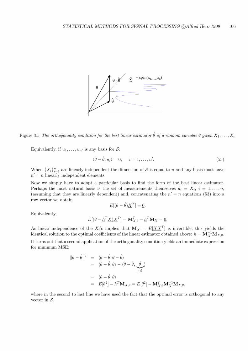
STATISTICAL METHODS FOR SIGNAL PROCESSING c©Alfred Hero 1999 106
θ
u1 θ - θ S
θ
= span(x1, …., xp)^
^
Figure 31: The orthogonality condition for the best linear estimator θ of a random variable θ given X1, . . . , Xn
Equivalently, if u1, . . . , un′ is any basis for S:
〈θ − θ, ui〉 = 0, i = 1, . . . , n′. (53)
When Xini=1 are linearly independent the dimension of S is equal to n and any basis must have
n′ = n linearly independent elements.
Now we simply have to adopt a particular basis to find the form of the best linear estimator.Perhaps the most natural basis is the set of measurements themselves ui = Xi, i = 1, . . . , n,(assuming that they are linearly dependent) and, concatenating the n′ = n equations (53) into arow vector we obtain
E[(θ − θ)XT ] = 0.
Equivalently,E[(θ − hT X)XT ] = MT
X,θ − hTMX = 0.
As linear independence of the Xi’s implies that MX = E[XXT ] is invertible, this yields theidentical solution to the optimal coefficients of the linear estimator obtained above: h = M−1
X MX,θ.
It turns out that a second application of the orthogonality condition yields an immediate expressionfor minimum MSE:
‖θ − θ‖2 = 〈θ − θ, θ − θ〉= 〈θ − θ, θ〉 − 〈θ − θ, θ︸︷︷︸
∈S〉
= 〈θ − θ, θ〉= E[θ2]− hTMX,θ = E[θ2]−MT
X,θM−1X MX,θ,
where in the second to last line we have used the fact that the optimal error is orthogonal to anyvector in S.
STATISTICAL METHODS FOR SIGNAL PROCESSING c©Alfred Hero 1999 107
5.4.2 AFFINE MINIMUM MSE ESTIMATION
The affine minimum MSE estimation problem is also easily cast into a vector space minimum normproblem. One way to do this is to subtract the mean from the parameter and subtract the meanfrom the measurements and proceed as in linear estimation - adding the parameter mean backinto the solution at the end. A more direct approach is to include the degenerate constant randomvariable ”1” into the measurement vector (we can always add a virtual sensor to the measurementsystem that measures a nonrandom constant!). To see how this would work first re-express theaffine estimator equation as
θ = hT X + b
= [hT , b][
X1
].
We now identify the solution subspace
S := spanX1, . . . , Xn, 1,which gives the following affine projection theorem:
Affine projection theorem: the best affine estimator of θ based r.v.s X1, . . . , Xn is the projectionof θ onto spanX1, . . . , Xn, 1.We leave it to the reader to verify that the aplication of the orthogonality condition to the pro-jection theorem gives the same solution that we derived before.
5.4.3 OPTIMALITY OF AFFINE ESTIMATOR FOR LINEAR GAUSSIAN MODEL
Introduce the addition assumption that X, θ are jointly Gaussian distributed. Then the minimumMSE estimator θ = θ(X) is in fact affine:
E[θ|X] = E[θ] + rTX,θR
−1X (X − E[X]).
One way to show this is to simply compute the conditional mean estimator and verify that it isin fact of the form of the affine estimator above. We take a different approach. Without loss ofgenerality, let’s specialize to the case of zero mean θ and X. Let θl be the LMMSE estimator,which is identical to the affine estimator in this case. From the linear projection theorem we knowthat the optimal estimator error is orthogonal to the measurements
E[(θ − θl)X] = 0
However, since θ − θl is a linear combination of Gaussian r.v.s it is itself Gaussian. Furthermore,since Gaussian r.v.s that are orthogonal are in fact independent r.v.’s
E[(θ − θl)|X] = E[(θ − θl)] = 0.
Therefore, as θl is a function of X we have
0 = E[(θ − θl)|X] = E[θ|X]− θl,
orE[θ|X] = θl
Which establishes the desired result.
STATISTICAL METHODS FOR SIGNAL PROCESSING c©Alfred Hero 1999 108
5.5 BEST AFFINE ESTIMATION OF A VECTOR
When the parameter θ = [θ1, . . . , θp]T is a vector it turns out that our previous results for scalarθ generalize very easily if we adopt the sum of the component MSEs as our error criterion. Definethe prior mean vector E[θ] and the cross-correlation matrix
RX,θ = cov(X, θ) = E[(x−E[X])(θ − E[θ])T ].
The sum MSE criterion is defined as
MSE(θ) =p∑
i=1
MSE(θi)
=p∑
i=1
E|θi − θi|2 = trace(E[(θ − θ) (θ − θ)T ]
).
Let the affine estimator θi of the i-th component of θ be defined by
θi = hTi X + bi, i = 1, . . . , p.
Define the affine vector estimator
θ = [θ1, . . . , θp]T = HT X + b
H = [h1, . . . , hp].
The affine minimum MSE vector estimation problem is to find H, b to minimize the sum MSEdenoted as MSE(H, b).
The solution is the optimal vector affine estimator
θ = E[θ] + Rθ,XR−1X (X − E[X]). (54)
The derivation of this result relies on the fact that each pair hi and bi appears separately in eachof the summands of MSE(θ). Hence the minimization of MSE is equivalent to the uncoupledminimization of each MSE(θi).
minθ
MSE(H, b) =p∑
i=1
minhi,bi
MSE(hi, bi).
Therefore the minimum MSE solution is simply the concatenation of the optimal scalar affineestimators of each θi:
θ1...θp
=
E[θ1]...
E[θp]
+
rθ1,XR−1X (X −E[X])
...rθp,XR−1
X (X − E[X])
,
which is equivalent to (54).
We can express the resultant minimum sum MSE as
MSEmin = trace(Rθ −Rθ,XR−1
X RX,θ
).
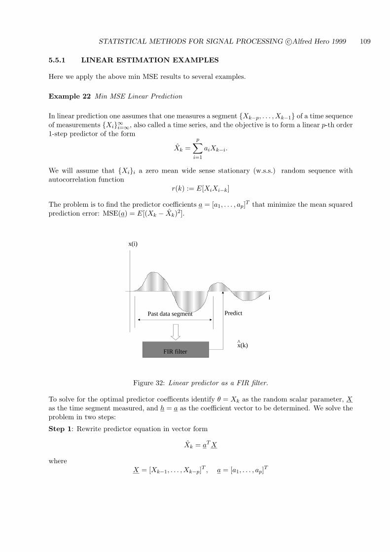
STATISTICAL METHODS FOR SIGNAL PROCESSING c©Alfred Hero 1999 109
5.5.1 LINEAR ESTIMATION EXAMPLES
Here we apply the above min MSE results to several examples.
Example 22 Min MSE Linear Prediction
In linear prediction one assumes that one measures a segment Xk−p, . . . , Xk−1 of a time sequenceof measurements Xi∞i=∞, also called a time series, and the objective is to form a linear p-th order1-step predictor of the form
Xk =p∑
i=1
aiXk−i.
We will assume that Xii a zero mean wide sense stationary (w.s.s.) random sequence withautocorrelation function
r(k) := E[XiXi−k]
The problem is to find the predictor coefficients a = [a1, . . . , ap]T that minimize the mean squaredprediction error: MSE(a) = E[(Xk − Xk)2].
i
x(i)
PredictPast data segment
FIR filter x(k)^
Figure 32: Linear predictor as a FIR filter.
To solve for the optimal predictor coefficents identify θ = Xk as the random scalar parameter, Xas the time segment measured, and h = a as the coefficient vector to be determined. We solve theproblem in two steps:
Step 1: Rewrite predictor equation in vector form
Xk = aT X
whereX = [Xk−1, . . . , Xk−p]T , a = [a1, . . . , ap]T
STATISTICAL METHODS FOR SIGNAL PROCESSING c©Alfred Hero 1999 110
Step 2: Express orthogonality condition as
E[(Xk − aT X)Xk−i] = 0, i = 1, . . . , p
or concatenation into a row vector gives
0T =
E[(Xk − aT X)Xk−1]...
E[(Xk − aT X)Xk−p]
= E[(Xk − aT X)XT ].
This specifies the optimal predictor coefficients a = a as
a = R−1r
where we have defined the correlation vector:
rT = [r1, . . . , rp] = E[XXk],
and the (Toeplitz) covariance matrix
R = ((r(i−j)))i,j=1,p = E[X XT ].
Finally, the predictor has minimum MSE
MSEmin = 〈Xk − aT X,Xk〉= r0 − aT r
= r0 − rTR−1r
Relation: The optimal linear predictor can be related to a so-called autoregressive order p (AR(p))model for Xi.To see this define residual prediction error Vk = Xk − Xk. Then, obviously
Xk = Xk + Vk =p∑
i=1
aiXk−i + Vk
When Vk is w.s.s. white noise the above representation is called an AR(p) model for Xi.
Example 23 An Inverse Problem
Assume a measurement model:X = Aθ + N
where
* X = [X1, . . . , Xm]T : random measurements
* θ = [θ1, . . . , θp]T : unknown random parameters
* N = [n1, . . . , nm]T : zero mean measurement noise with covariance RN
* θ,N uncorrelated
* A: a known m× p matrix
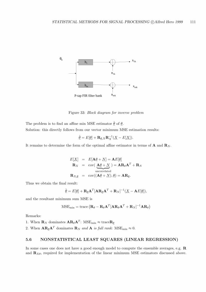
STATISTICAL METHODS FOR SIGNAL PROCESSING c©Alfred Hero 1999 111
θκ
hm
h1
n1k
nmk
x1k
xmk
P-tap FIR filter bank
Figure 33: Block diagram for inverse problem
The problem is to find an affine min MSE estimator θ of θ.
Solution: this directly follows from our vector minimum MSE estimation results:
θ = E[θ] + Rθ,XR−1X (X − E[X]).
It remains to determine the form of the optimal affine estimator in terms of A and RN .
E[X] = E[Aθ + N ] = AE[θ]RX = cov( Aθ + N︸ ︷︷ ︸
uncorrelated
) = ARθAT + RN
RX,θ = cov((Aθ + N), θ) = ARθ.
Thus we obtain the final result:
θ = E[θ] + RθAT [ARθAT + RN ]−1(X −AE[θ]),
and the resultant minimum sum MSE is
MSEmin = trace(Rθ −RθAT [ARθAT + RN ]−1ARθ
)
Remarks:
1. When RN dominates ARθAT : MSEmin ≈ traceRθ
2. When ARθAT dominates RN and A is full rank: MSEmin ≈ 0.
5.6 NONSTATISTICAL LEAST SQUARES (LINEAR REGRESSION)
In some cases one does not have a good enough model to compute the ensemble averages, e.g. Rand RXθ, required for implementation of the linear minimum MSE estimators discussed above.
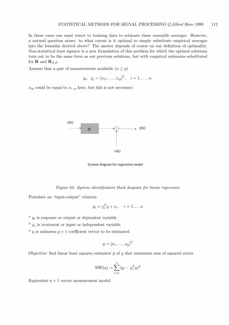
STATISTICAL METHODS FOR SIGNAL PROCESSING c©Alfred Hero 1999 112
In these cases one must resort to training data to estimate these ensemble averages. However,a natural question arises: to what extent is it optimal to simply substitute empirical averagesinto the formulas derived above? The answer depends of course on our definition of optimality.Non-statistical least squares is a new formulation of this problem for which the optimal solutionsturn out to be the same form as our previous solutions, but with empirical estimates substitutedfor R and RX,θ.
Assume that a pair of measurements available (n ≥ p)
yi, xi = [xi1, . . . , xip]T , i = 1, . . . , n.
xip could be equal to xi−p here, but this is not necessary.
a
x(k)
v(k)
y(k)
System diagram for regression model
Figure 34: System identification block diagram for linear regression
Postulate an “input-output” relation:
yi = xTi a + vi, i = 1, . . . n
* yi is response or output or dependent variable
* xi is treatment or input or independent variable
* a is unknown p× 1 coefficient vector to be estimated
a = [a1, . . . , ap]T
Objective: find linear least squares estimator a of a that minimizes sum of squared errors
SSE(a) =n∑
i=1
(yi − xTi a)2
Equivalent n× 1 vector measurement model:
STATISTICAL METHODS FOR SIGNAL PROCESSING c©Alfred Hero 1999 113
y1,...
yn
=
xT1...
xTn
a +
v1,...
vn
y = Xa + v,
where X is a non-random n× p input matrix.
The estimation criterion is
SSE(a) = (y −Xa)T (y −Xa)
Solution to LLSE of a:
Step 1. Identify vector space containing y: H = IRn
Inner product: 〈y, z〉 = yT z
Step 2. Identify solution subspace containing Xa
S = spancolumns of X
which contains vectors of form
Xa =p∑
k=1
ak
[x1k, . . . , xnk
]T
Step 3. apply projection theorem
Orthogonality Condition: the best linear estimator a satisfies
〈y −Xa, ui〉 = 0, i = 1, . . . , n
where ui are columns of X, or equivalently
0T = (y −Xa)TX
= yTX− aT XTX
or, if X has full column rank p then XTX is invertible and
a = [XTX]−1 XT y
= [n−1XTX]−1 [n−1XT ]y
= R−1x rxy.
Here
Rxdef=
1n
n∑
i=1
xi xTi , rxy
def=1n
n∑
i=1
xi yi

STATISTICAL METHODS FOR SIGNAL PROCESSING c©Alfred Hero 1999 114
We next specify the projection operator form of predicted output response
y = Xa
which, using above, can be represented as the orthogonal projection of y onto S
y = Xa
= X[XTX]−1 XT y
= X[XTX]−1XT
︸ ︷︷ ︸orthog. projection
y
Properties of orthogonal projection operator:
ΠX = X[XTX]−1XT
Property 1. ΠX projects vectors onto column space of X
Define decomposition of y into components yX
in column space of X and y⊥X
orthogonal to columnspace of X
y = yX
+ y⊥X
Then for some vector α = [α1, . . . , αp]T
Column span X
y
yx
yx⊥
Figure 35: Column space decomposition of a vector y
yX
= Xα, XT y⊥X
= 0
STATISTICAL METHODS FOR SIGNAL PROCESSING c©Alfred Hero 1999 115
We have:
ΠXy = ΠX(yX
+ y⊥)
= X [XTX]−1XTX︸ ︷︷ ︸=I
α + X[XTX]−1 XT y⊥X︸ ︷︷ ︸
=0
= Xα
= yX
so that ΠX extracts the column space component of y. Thus we can identify yX
= ΠXy so thatwe have the representation
y = ΠXy + (I −ΠX)y︸ ︷︷ ︸y⊥X
It follows immediately that 2. I −ΠX projects onto the space orthogonal to spancolsX3. ΠX is symmetric and idempotent: ΠT
XΠX = Π
4. (I −ΠX)ΠX = 0
Projection operator form of LS estimator gives alternative expression for minimum SSE
SSEmin = (y − y)T (y − y)
= yT [I −ΠX]T [I −ΠX]y
= yT [I −ΠX]y
Example 24 LS optimality of sample mean
Measure x = [x1, . . . , xn]T
Objective: Find best constant c which minimizes the sum of squares
n∑
k=1
(xi − c)2 = (x− c1)T (x− c1)
where 1 = [1, . . . , 1]T
Step 1: identify solution subspace
S is diagonal line: y : y = a1, a ∈ IRStep 2. apply orthogonality condition
(x− c1)T 1 = 0 ⇐⇒ c =xT 11T 1
= n−1n∑
k=1
xi
Example 25 LLS linear prediction from training sample

STATISTICAL METHODS FOR SIGNAL PROCESSING c©Alfred Hero 1999 116
1
1
1
1=[1, …, 1]T
S
Figure 36: Diagonal line is solution subspace for LS scalar
i
x(i)
PredictPast data segment
FIR filter x(k)^
Training sequence for constructing FIR predictor
Figure 37: Construction of LLS predictor from training sequence
STATISTICAL METHODS FOR SIGNAL PROCESSING c©Alfred Hero 1999 117
Measurement sequence ziTraining sequence of n + p samples of zi
zip+ni=1 , i = 1, . . . , n
Fit an AR(p) model to training sequence
zk =p∑
i=1
aizk−i + vk, k = p + 1, . . . , n
such that SSE is minimized
SSE(n) =n∑
k=1
(zk+p −p∑
i=1
aizk+p−i)2
Solution
Step 1. Identify response variables yk = zk and input vectors zk = [zk−1, . . . , zk−p]T .
zn+p,...
zp+1
=
zTn+p,...
zTp+1
a +
vn+p...
vp+1
y = Xa + v,
Step 2. Apply orthogonality condition
The LLS p-th order linear predictor is of the form:
zk =p∑
i=1
aizk−i
where a = [a1, . . . , ap]T is obtained from formula
a = [XTX]−1XT y = R−1 r
and we have defined the sample correlation quantities:
r = [r1, . . . , rp]T
R = ((r(i− j)))i,j=1,p
rj := n−1n∑
i=1
zi+pzi+p−j , j = 0, . . . , p
STATISTICAL METHODS FOR SIGNAL PROCESSING c©Alfred Hero 1999 118
5.7 LINEAR MINIMUM WEIGHTED LEAST SQUARES ESTIMATION
As before assume linear model for input and response variables
y1,...
yn
=
xT1 ,...
xTn
a +
v1,...
vn
y = Xa + v,
The linear minimum weighted least squares (LMWLS) estimator a of a minimizes
SSE(a) = (y −Xa)T W (y −Xa)
where W is a symmetric positive definite n× n matrix
Solution to LMWMS problem:
Step 1. Identify vector space containing y: H = IRn
Inner product: 〈y, z〉 = yT Wz
Step 2. Identify solution subspace S
Xa = spancolumns of X
Step 3. apply projection theorem
Orthogonality Condition: the best linear estimator a satisfies
0 = (y −Xa)TWX
= yTWX− aT XTWX
or, if X has full column rank p then XTWX is invertible and
a = [XTWX]−1XTWy
5.7.1 PROJECTION OPERATOR FORM OF LMWLS PREDICTOR
The vector y of least squares predictors yi = xTi a of the actual output y is
y = Xa
which can be represented as the “oblique” projection of y onto H
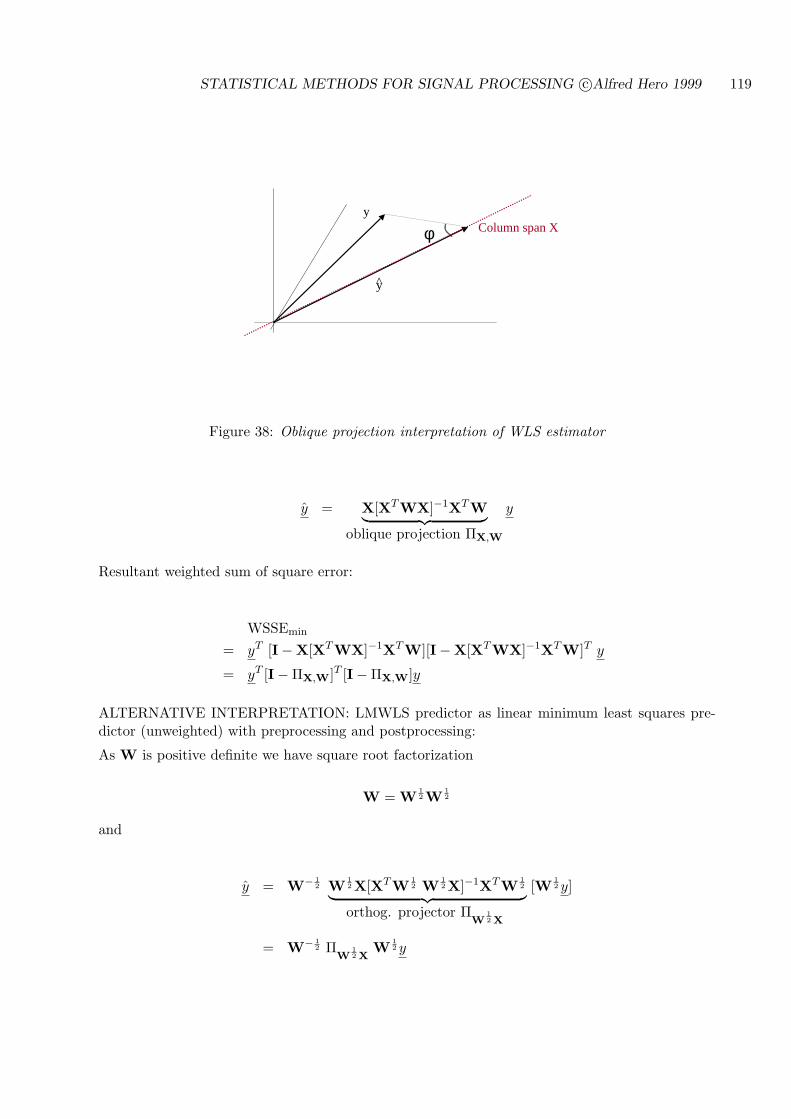
STATISTICAL METHODS FOR SIGNAL PROCESSING c©Alfred Hero 1999 119
Column span Xφ
y
y
^
Figure 38: Oblique projection interpretation of WLS estimator
y = X[XTWX]−1XTW︸ ︷︷ ︸oblique projection ΠX,W
y
Resultant weighted sum of square error:
WSSEmin
= yT [I−X[XTWX]−1XTW][I−X[XTWX]−1XTW]T y
= yT [I−ΠX,W]T [I−ΠX,W]y
ALTERNATIVE INTERPRETATION: LMWLS predictor as linear minimum least squares pre-dictor (unweighted) with preprocessing and postprocessing:
As W is positive definite we have square root factorization
W = W12 W
12
and
y = W− 12 W
12 X[XTW
12 W
12 X]−1XTW
12︸ ︷︷ ︸
orthog. projector ΠW
12 X
[W12 y]
= W− 12 Π
W12 X
W12 y
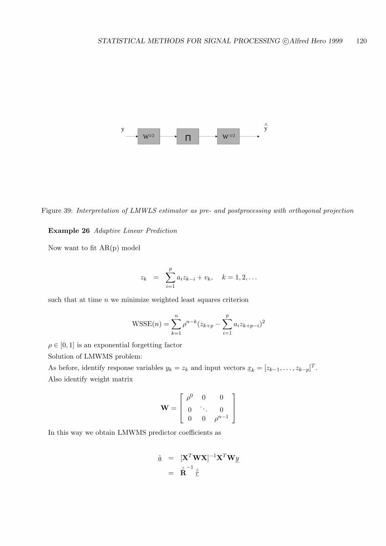
STATISTICAL METHODS FOR SIGNAL PROCESSING c©Alfred Hero 1999 120
^y y
W1/2 W-1/2Π
Figure 39: Interpretation of LMWLS estimator as pre- and postprocessing with orthogonal projection
Example 26 Adaptive Linear Prediction
Now want to fit AR(p) model
zk =p∑
i=1
aizk−i + vk, k = 1, 2, . . .
such that at time n we minimize weighted least squares criterion
WSSE(n) =n∑
k=1
ρn−k(zk+p −p∑
i=1
aizk+p−i)2
ρ ∈ [0, 1] is an exponential forgetting factor
Solution of LMWMS problem:
As before, identify response variables yk = zk and input vectors xk = [zk−1, . . . , zk−p]T .
Also identify weight matrix
W =
ρ0 0 0
0. . . 0
0 0 ρn−1
In this way we obtain LMWMS predictor coefficients as
a = [XTWX]−1XTWy
= ˆR−1
ˆr
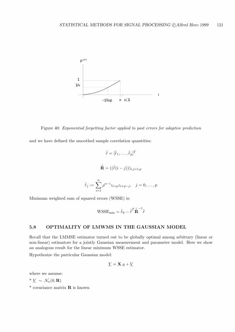
STATISTICAL METHODS FOR SIGNAL PROCESSING c©Alfred Hero 1999 121
n
1/e1
−1/lnρ n+1
ρ n-i
i
Figure 40: Exponential forgetting factor applied to past errors for adaptive prediction
and we have defined the smoothed sample correlation quantities:
ˆr = [ˆr1, . . . , ˆrp]T
ˆR = ((ˆr(i− j)))i,j=1,p
ˆrj :=n∑
i=1
ρn−izi+pzi+p−j , j = 0, . . . , p
Minimum weighted sum of squared errors (WSSE) is:
WSSEmin = ˆr0 − ˆrT ˆR
−1ˆr
5.8 OPTIMALITY OF LMWMS IN THE GAUSSIAN MODEL
Recall that the LMMSE estimator turned out to be globally optimal among arbitrary (linear ornon-linear) estimators for a jointly Gaussian measurement and parameter model. Here we showan analogous result for the linear minimum WSSE estimator.
Hypothesize the particular Gaussian model:
Y = X a + V
where we assume:
* V ∼ Nn(0,R)
* covariance matrix R is known

STATISTICAL METHODS FOR SIGNAL PROCESSING c©Alfred Hero 1999 122
n
Steady state
Figure 41: Typical trajectory of the error criterion for predicting a stationary AR(1) process
* X is known non-random matrix of measurements
Under the above hypothesis, for any given X or a the density function of Y is multivariate Gaussian
f(y; a) =1√
(2π)n|R| exp(−1
2(y −Xa)TR−1(y −Xa)
).
This implies that the maximum likelihood (ML) estimator of a is identical to the LMWMS esti-mator. To see this express
aml = argmaxa ln f(Y ; a)
= argmina(Y −Xa)TR−1(Y −Xa).
Hence
Y = Xaml = X[XTR−1X]−1XTR−1Y = ΠX,W Y .
Under the hypothesized model we can evaluate estimator performance by looking to satisfy thecondition for equality in the Cramer-Rao bound (CRB)
(∇a ln f)T = (Y −Xa)T R−1X
=
Y TR−1X[XTR−1X]−1
︸ ︷︷ ︸aT
−aT
XTR−1X︸ ︷︷ ︸
Ka
We conclude: when X is nonrandom and noise covariance R is known to be equal to the LSweighting matrix W−1 then
* the LMWMS estimator a is unbiased
* the LMWMS estimator is efficient and therefore UMVUE

STATISTICAL METHODS FOR SIGNAL PROCESSING c©Alfred Hero 1999 123
* recalling property 5 of the CRB in Section 4.5.1, as Ka is not a function of a the estimatorcovariance is
cova(a) = K−1a = [XTR−1X]−1 = ˆR
−1 1n
5.9 BACKGROUND REFERENCES
Two classic statistical references for linear estimation are Rao [56] and Anderson [2]. For treat-ments with more of a signal processing flavor the reader is referred to books by Scharf [59], VanTrees [72] and Kay [36]. The area of control and systems identification have also developed theirown distinctive approaches to this problem, see Kailath [32] and Soderstrom and Stoica [65].
5.10 APPENDIX: VECTOR SPACES
For a concise overview of vector spaces in the context of signal processing the reader is referred toMoon and Stirling [48]. For a more advanced treatment with an orientation towards optimizationsee Luenberger [41].
Definition: H is a vector space over a scalar field F if for any elements x, y, z ∈ H and scalarsα, β ∈ F1. α · x + β · y ∈ H (Closure)
2. x + (y + z) = (x + y) + z
3. α · (x + y) = α · x + α · y4. (α + β) · x = α · x + β · x5. There is a vector φ ∈ H s.t.: x + φ = x
6. There are scalars 1, 0 s.t.: 1 · x = x, 0 · x = φ
A normed vector space H has an inner product 〈·, ·〉 and a norm ‖ · ‖ which satisfy
1. 〈x, y〉 = 〈y, x〉∗2. 〈α · x, y〉 = α∗〈x, y〉3. 〈x + y, z〉 = 〈x, z〉+ 〈y, z〉4. ‖x‖2 = 〈x, x〉5. ‖x‖ ≥ 0
6. ‖x‖ = 0 iff x = φ
7. ‖x + y‖ ≤ ‖x‖+ ‖y‖ (Triangle ineq)
8. |〈x, y〉| ≤ ‖x‖ ‖y‖ (Cauchy-Schwarz ineq)
9. Angle between x, y: ψ = cos−1( 〈x,y〉‖x‖ ‖y‖
)
10. 〈x, y〉 = 0 iff x, y are orthogonal
11. |〈x, y〉| = ‖x‖ ‖y‖ iff x = α · y for some α
12. The linear span of vectors x1, . . . , xk is
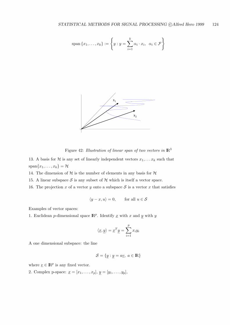
STATISTICAL METHODS FOR SIGNAL PROCESSING c©Alfred Hero 1999 124
span x1, . . . , xk :=
y : y =
k∑
i=1
αi · xi, αi ∈ F
x1
x2
Figure 42: Illustration of linear span of two vectors in IR3
13. A basis for H is any set of linearly independent vectors x1, . . . xk such that
spanx1, . . . , xk = H14. The dimension of H is the number of elements in any basis for H15. A linear subspace S is any subset of H which is itself a vector space.
16. The projection x of a vector y onto a subspace S is a vector x that satisfies
〈y − x, u〉 = 0, for all u ∈ S
Examples of vector spaces:
1. Euclidean p-dimensional space IRp. Identify x with x and y with y
〈x, y〉 = xT y =p∑
i=1
xiyi
A one dimensional subspace: the line
S = y : y = av, a ∈ IR
where v ∈ IRp is any fixed vector.
2. Complex p-space: x = [x1, . . . , xp], y = [y1, . . . , yp],
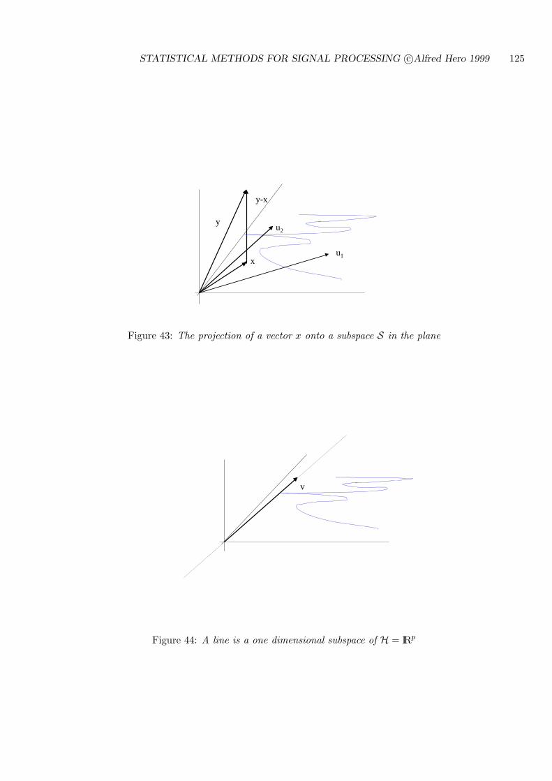
STATISTICAL METHODS FOR SIGNAL PROCESSING c©Alfred Hero 1999 125
x
y
y-x
u1
u2
Figure 43: The projection of a vector x onto a subspace S in the plane
v
Figure 44: A line is a one dimensional subspace of H = IRp
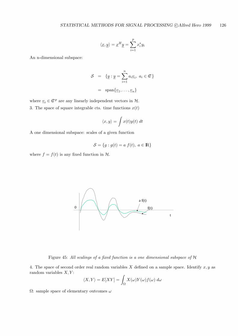
STATISTICAL METHODS FOR SIGNAL PROCESSING c©Alfred Hero 1999 126
〈x, y〉 = xHy =p∑
i=1
x∗i yi
An n-dimensional subspace:
S = y : y =n∑
i=1
aivi, ai ∈ Cl
= spanv1, . . . , vn
where vi ∈ Cl p are any linearly independent vectors in H.
3. The space of square integrable cts. time functions x(t)
〈x, y〉 =∫
x(t)y(t) dt
A one dimensional subspace: scales of a given function
S = g : g(t) = a f(t), a ∈ IR
where f = f(t) is any fixed function in H.
0 f(t)
t
a f(t)
Figure 45: All scalings of a fixed function is a one dimensional subspace of H
4. The space of second order real random variables X defined on a sample space. Identify x, y asrandom variables X,Y :
〈X, Y 〉 = E[XY ] =∫
ΩX(ω)Y (ω)f(ω) dω
Ω: sample space of elementary outcomes ω
STATISTICAL METHODS FOR SIGNAL PROCESSING c©Alfred Hero 1999 127
Q. How to use vector spaces for estimation?
A. Identify H = Y : Y a r.v. with E[|Y |2]〈∞.Inner product beween two “vectors” in H is defined as
〈X,Y 〉 := E[XY ]
(X,Y real r.v.s)
5.11 EXERCISES
5.1 Give a concrete example of two zero mean random variables X and Z for which the linearminimum mean square error estimator of X given Z is equal to 0. Give another concreteexample where the overall (linear or non-linear) minimum mean square error estimator is 0.
5.2 Here you explore how linear minimum MSE estimation principles can be applied to non-linearestimation. Given an observed random variable X define the vector of monomials in X:
Y = [1, X, X2, . . . , Xm]T ,
where m ≥ 1 is a positive integer. A non-linear polynomial estimator of order m of anotherrandom variable θ given observation X is simply a linear combination of the elements of Y :
θ = hT Y ,
where h = [h0, . . . , hm]T is a set of estimation coefficients to be determined. For questions (b)and (c) you may find is useful to use the following facts about a zero mean Gaussian randomvariable Z: E[Zk] = 0 if k is odd integer while otherwise E[Zk] = σk
Z · (k− 1) · (k− 3) · · · 3 · 1.Also E[|Z|] = σZ
√2/π.
(a) What is the choice of h that minimizes the MSE E[(θ− θ)2]? What is the mean squarederror of the resulting optimal non-linear polynomial estimator?
(b) Let X = sgn(S) + W , where sgn(u) is the sign of u, S, W are uncorrelated, jointlyGaussian and zero mean. Find the optimal first order (m = 1) estimator of S givenmeasurement of X and its resulting minimum MSE. This is the standard optimal linear(affine) estimator we have studied in class.
(c) For the same measurement model for X as in part (b) find the optimal second order(m = 2) non-linear polynomial estimator of S in terms of σ2
w and σ2s .
5.3 The least squares method can also be applied to multiple-response linear observation modelsof the form
y1k + α1y2k . . . + αp−1ypk = β1x1k + . . . + βqxqk + vk, k = 1, . . . , n
where y1k, . . . , ypkk are n different observed waveforms (responses) and the αi. and βi
coefficients are to be determined by minimizing the least squares criterion
SSE(α, β) =n∑
k=1
(yk + α1y2k + . . . + αp−1ypk − β1x1k − . . .− βqxqk)2
STATISTICAL METHODS FOR SIGNAL PROCESSING c©Alfred Hero 1999 128
(a) Show that the above observation model is equivalent to the vector model
Y [1, αT ]T = Xβ + v
where Y and X are n× p and n× q matrices, respectively, v is a n× 1 vector of residualsvk, α = [α1, . . . , αp−1]T and β = [β1, . . . , βq]T .
(b) Assuming that X has linearly independent columns (full rank) find the least squaresestimates β and α and the resulting minimum SSE. (Hint: first minimize over β thenover α)
(c) Assume that the vector u = [1, α]T is constrained to have length ‖u‖ = c, where c ≥ 1is a specified constant. Derive an explicit form for the LS estimators. (Hint: Rayleightheorem (Ch. 2 or [19]) on minimizing quadratic forms).
(d) The “sensor selection problem” is the following. Fix p′and consider choosing the subset
of p′response waveforms yi1,kn
k=1, . . . , yip′ ,kn
k=1, i1, . . . , ip′ distinct integers in 1. . . . , p,out of the p responses which provide the best fit, i.e. minimize the residuals. Show thatthe algorithm for solving this sensor selection problem requires solving p!/(p
′!(p − p
′))!
separate least squares problems.(e) The optimal sensor selection algorithm which you obtained in the previous part of this
exercise is of high computational complexity, in the worst case it requires solving approx-imately pp
′least squares problems. Comment on how the solutions to parts (b) or (c) of
this exercise could be used to approximate the optimal solution.
5.4 Let the observation have the standard linear model yk = xTk a + vk, k = 1, . . . , n. We
saw in this chapter that when yk and xk are known and vk is Gaussian the MLE of a isequivalent to the WLSE with weight matrix equal to the covariance matrix of the vectorv = [v1, . . . , vn]T . In many applications there exist outliers, i.e. a small number of unusuallylarge residual errors vk, and the Gaussian assumption is not appropriate. Here we treat thecase of heavy-tailed distributions of vk which leads to an estimate of a which is more robustto outliers.
(a) Assume that vk are i.i.d. r.v.s with marginal density fv(v). Show that the MLE of a is
a = argmina
n∑
k=1
log fv(yk − xTk a)
(b) Assuming fv is a smooth function, derive the CR bound on unbiased estimators of a.Under what conditions is the bound attainable?
(c) Show that for Laplacian noise with fv(v) = β2 exp(−β|v|), β ≥ 0, the MLE reduces to
the minimizer of the sum of the absolute errors |yk − xTk a|.
(d) Consider the noise density fv(v) = c(α, b) exp(−v2/(α2 + v2)), v ∈ [−b, b], b and α fixedknown parameters and c a normalizing constant. Show that the MLE a can be interpretedas a non-linearly weighted LSE in the sense that it satisfies the “orthogonality condition”
n∑
k=1
λk(a)(yk − xTk a)xk = 0
whereλk(a) =
1α2 + (yk − xT
k a)2
STATISTICAL METHODS FOR SIGNAL PROCESSING c©Alfred Hero 1999 129
(e) The solution to the non-linearly weighted LSE above can be approximated using an“iterative reweighted least squares” technique which consists of approximating the above“orthogonality condition” by implementing the following procedurei. Initialize a0 = a equal to the standard unweighted LS estimate a = [XT X]XT y.ii. Repeat until convergence:
ai+1 = [XT WiX]−1XT Wiy, i = 1, 2, . . .
where Wi is a diagonal weight matrix with diagonal entries λ1(ai), . . . , λn(ai).Implement this algorithm in MATLAB and study its convergence for various values ofα, b.
5.5 In many applications involving fitting a model to a set of input and output measurements X(n×p) and y (n×1), not only are the output measurements noisy but the input measurementsmay also be noisy. In this case the method of Total Least Squares (TLS) [19] is applicable.One formulation of TLS is to model the measurements by
yk = (xk + εk)T a + vk, k = 1, . . . , n
where vk is a zero mean white Gaussian noise with variance σ2v and εk is an i.i.d. sequence of
zero mean Gaussian p× 1 random vectors with diagonal covariance matrix σ2ε Ip.
(a) Find the likelihood equation which must be satisfied by the MLE of a when σv and σε
are known. To what does your equation reduce when σ2v dominates σ2
ε ? What is the MLestimator for a in this case?
(b) Show that the MLE of a is identical to the standard LS estimator for unknown σε.(c) Find the Fisher information and the CR bound on unbiased estimator covariance for the
case of known σv and σε. Repeat for the case of unknown σε. For which of these cases,if any, is the CR bound achievable?
5.6 It is desired to find the linear least sum of squares (LLSS) fit of a complex valued vector ato the model
yk = xTk a + vk, k = 1, . . . , n
where yk and xk = [xk1, . . . , xkp]T are observed. Defining the vector space H of complexvalued n-dimensional vectors with norm < y, z >= yHz (“H” denotes complex conjugatetranspose) and vector y = [y1, . . . , yn]T and matrix X = [x1, . . . , xn]T (analogously to thecase studied in sec. 5.6 of notes). Assume that X is full rank. Using the projection theoremshow that the solution to the LLSE problem mina ‖y −Xa‖2 is of the form
a = [XHX]−1XHy
with minimum LLSS residual error squared
‖y −Xa‖2 = yH [I −X[XHX]−1XH ]y.
5.7 This problem applies the solution to the previous exercise. Let the complex observations begiven as X = X(0), . . . , X(N−1). Hypothesize that X(k) is a damped sinusoid in additivenoise:
X(k) = ae−αkej2πf0k + Z(k), k ≥ 0,
where a ∈ Cl is an unknown complex scale factor, α ≥ 0 is an unknown decay constant, andf0 ∈ [0, 1
2 ] is an unknown frequency.
STATISTICAL METHODS FOR SIGNAL PROCESSING c©Alfred Hero 1999 130
(a) For known α and f0 show that the least-squares estimator of a which minimizes the sumof the squared residuals SSE(a) =
∑N−1k=0 |X(k) − ae−αkej2πf0k|2 over a has the form
(large N):a = X (z0) (1− e−2α),
where X (z0) =∑N−1
k=0 X(k)z−k0 is the Z-transform of X evaluated at the point z = z0 =
eα+j2πf0 outside the unit circle. Note that for α = 0 this is just the DFT of X(k).(b) Now for known α but unknown a show that the (non-linear) least-squares estimator for f0
which minimizes the sum of the squared residuals SSE(a) =∑N−1
k=0 |X(k)−ae−αkej2πf0k|2over fo is obtained by maximizing the Z-transform of X over the radius eα circle |z| = eα:
f0 = argmaxf0|X (z0)|2 ,
and:a = X (eα+j2πf0) (1− e−2α).
Note that f0 reduces to the location of the highest peak in the magnitude “frequencyspectrum” S(f) =
∣∣X (e2πf )∣∣ of X(k) when α is known to be equal to 0.
(c) Finally for unknown a, α, f0 show that the non-linear least-squares estimator of α, f0 isobtained by maximizing the scaled Z-transform of X over the exterior of the unit disk:
f0, α = argmaxf0,α≥0 |X (z0)|2 (1− e−2α),
and:a = X (eα+j2πf0) (1− e−2α).
5.8 It is desired to fit the coefficients α and β to the linear model for the measurements yk =α + βk + vk, k = 1, . . . , N , where vk is the model error residual to be minimized by suitablechice of α, β. Find the linear least squares estimator for these coefficents (you can leave yoursolution in the form of a pair of simultaneous equations if you wish).
5.9 It is hypothesized that the relation between a pair of measured variables yk and xk is non-linear. A reasonable model for this is
yk = a0 + a1xk + . . . + apxp + vk, k = 1, . . . , n
(a) For a single sample (n = 1) find the set of coefficients a0, . . . , ap which minimizes themean squared error E[(yk− [a0 + a1xk + . . .+ apx
p])2] under the assumption that yk andxk are r.v.’s with known moments E[ykx
lk], l = 0, . . . , p, and E[xl
k], l = 0, . . . , 2p.(b) Repeat part (a) for the non-statistical least squares estimation error criterion for n sam-
ples∑n
k=1(yk − [a0 + a1xk + . . . + apxp])2 .
(c) Show that the two estimators found in (a) and (b) become equivalent as n →∞.
5.10 A sequence of obervations yk, k = 1, . . . , N is to be modeled as the sum of two sinusoids
yk = A cos(ωok) + B sin(ωok) + vk
where vk is an error residual, ω is known, and A,B are to be determined.
(a) Derive the linear least squares estimators of A,B. Express your result in terms of thereal and imaginary parts of the DFT Y(ω) =
∑Nk=1 yke
−jωk of yk. You may assume that∑Nk=1 cos(2ωok) =
∑Nk=1 sin(2ωok) = 0.
STATISTICAL METHODS FOR SIGNAL PROCESSING c©Alfred Hero 1999 131
(b) Now assume that A and B are uncorrelated r.v.s with mean µA and µB and variance σ2
and that vk is zero mean white noise of unit variance uncorrelated with A,B. Derive theaffine minimum mean square error estimator of A,B given yk, k = 1, . . . , N .
(c) Express the result of (b) in terms of the real and imaginary parts of the DFT Y(ω) =∑Nj=1 yke
−jωk of yk and compare to the result of part (a)
5.11 In this problem you will explore least squares deconvolution. Available for measurement arethe noisy outputs Yk, k = 1, . . . , n, of a known LTI filter (channel), with known finite impulseresponse hkp
k=0 and having an unknown input Xk, and measured in additive noise Wk
Yk =p∑
i=0
hiXk−i + Wk, k = 1, . . . , n
The objective is to deconvolve the measurements using the known channel hk to recoverthe input Xk. Assume that Xk = 0 for k ≤ 0.
(a) Show that the above measurement equation can be put in the form
Y = HX + W,
where H is a matrix of impulse responses of the FIR filter. Identify the entries of thevectors X, W and the matrix H.
(b) Assuming that H has linearly independent columns (full rank) find the linear least squaresestimate X which minimizes the sum of squared errors
∑nk=1(Yk−hk∗Xk)2 (“ * ” denotes
convolution). Give a relation on p, n or hi to ensure that H has full rank.(c) In some cases estimation errors in the recent past are more important than errors in the
more distant past. Comment on how you would incorporate this into a weighted linearleast squares criterion and find the criterion-minimizing linear estimator X.
(d) A simple model for imprecise knowledge of the channel is
Y = (H + zI)X + W
where z is a zero mean Gaussian random variable with variance σ2. Assuming that Wis zero mean Gaussian random vector with identity covariance (I) find the likelihood
function for θdef= X based on the observation Y . Show that the ML estimator reduces
to the linear least squares estimate of part (b) when σ2 → 0.
End of chapter
STATISTICAL METHODS FOR SIGNAL PROCESSING c©Alfred Hero 1999 132
6 OPTIMAL LINEAR FILTERING AND PREDICTION
In the last chapter linear and affine estimation was explored for the case of a small number n ofmeasurements, or at least small enough so that the n×n covariance matrix RX could be invertedpermitting implementation of the linear minimum mean squared error estimator. In this chapterwe turn to the case where an online linear predictor is desired, the number n of measurementsis increasing over time, and matrix inversion quickly becomes impractical. This situation arisesin many signal processing applications where ”streaming data” is collected. The approach thatis taken for this problem is to model the measurements as coming from a random process withknown autocorrelation function (acf). Under some additional assumptions on the acf the linearpredictors can be implemented recursively by applying a filter to the data stream. In Wienerfiltering, designed for wide sense stationary (wss) processes, this filter is causal and linear timeinvariant (LTI) while in Kalman-Bucy filtering, designed for non-stationary processes, the filter islinear time varying (LTV).
We will cover the following topics.
* Wiener-Hopf Equations of min MSE filtering for w.s.s. processes
* Non-causal filtering, estimation, and prediction
* Causal LTI prewhitening: spectral factorization
* Causal LTI prediction: the Wiener filter
* Causal LTV prewhitening: the innnovations filter
* Causal LTV prediction: the Kalman-Bucy filter
A word about notation is in order here. Up to now in this text we have used upper case lettersfor random variables reserving lower case for their realizations. However, it is customary to dropthe upper case for random processes and we will do so in this chapter putting the reader at smallrisk of confusion between realizations, i.e. waveforms, and random processes. Fortunately, secondorder statistical treatments like that covered here incur fewer accidents due to this kind of abuseof notation.
6.1 WIENER-HOPF EQUATIONS OF OPTIMAL FILTERING
The Wiener filter is useful for linear prediction when one assumes with wss processes. The deriva-tion of the filter below requires some facility with z-domain power spectral densities (PSD) forwhich the reader is referred to the Appendix, Sec. 6.13.
Two zero mean w.s.s. discrete time random processes x and g are of interest to us:
* x = xk : k ∈ I: observed over an index set I* g = gk : −∞ < k < ∞: unobserved and to be estimated from x
Objective: estimate a time sample of g, e.g. gi, by a linear function of the waveform x. Note thatgk plays the role of a random parameter, which we denoted θk in previous chapters.
gk =∑
j∈Ih(k, j)xj
such that we achieve minimum MSE over choice of linear coefficients h = h(k, jk,j :
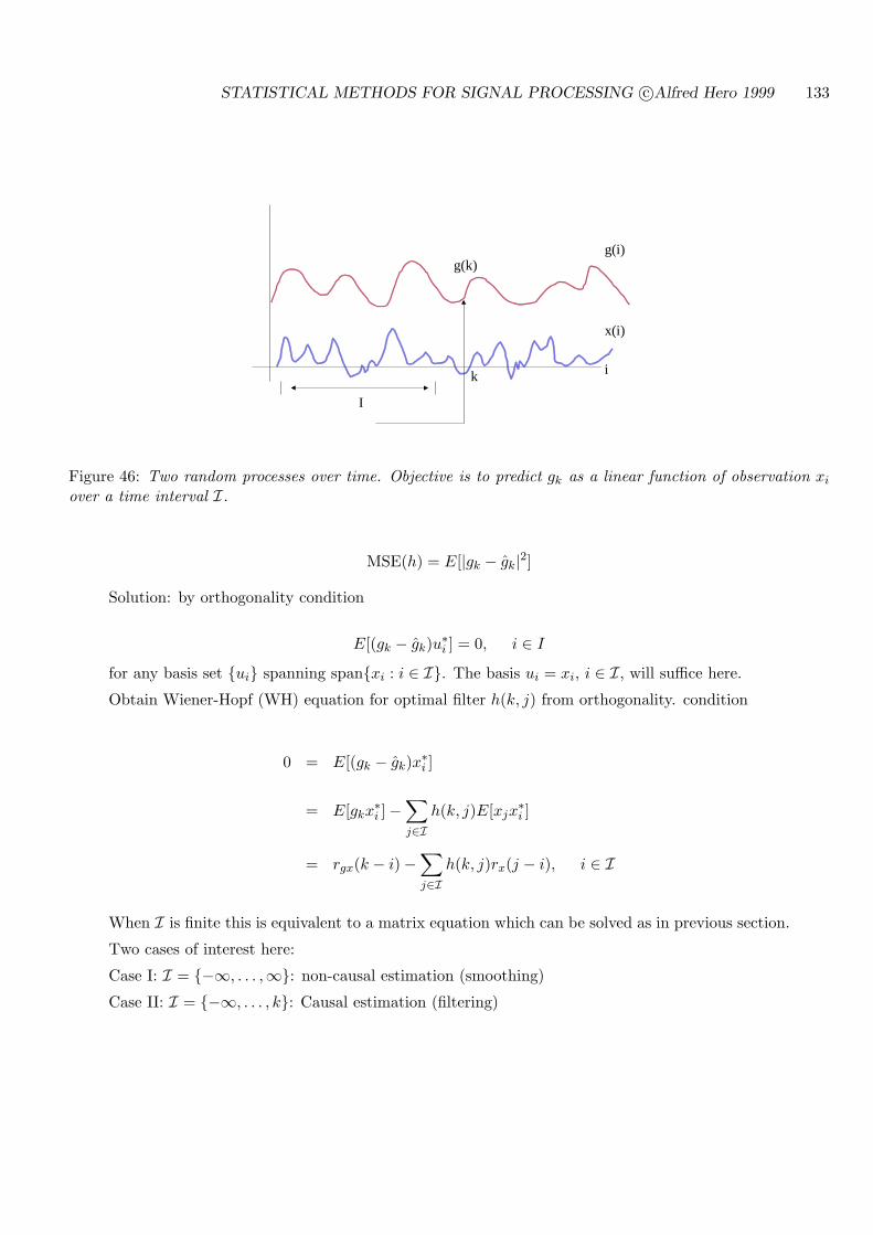
STATISTICAL METHODS FOR SIGNAL PROCESSING c©Alfred Hero 1999 133
I
i
g(i)
x(i)
k
g(k)
Figure 46: Two random processes over time. Objective is to predict gk as a linear function of observation xi
over a time interval I.
MSE(h) = E[|gk − gk|2]
Solution: by orthogonality condition
E[(gk − gk)u∗i ] = 0, i ∈ I
for any basis set ui spanning spanxi : i ∈ I. The basis ui = xi, i ∈ I, will suffice here.
Obtain Wiener-Hopf (WH) equation for optimal filter h(k, j) from orthogonality. condition
0 = E[(gk − gk)x∗i ]
= E[gkx∗i ]−
∑
j∈Ih(k, j)E[xjx
∗i ]
= rgx(k − i)−∑
j∈Ih(k, j)rx(j − i), i ∈ I
When I is finite this is equivalent to a matrix equation which can be solved as in previous section.
Two cases of interest here:
Case I: I = −∞, . . . ,∞: non-causal estimation (smoothing)
Case II: I = −∞, . . . , k: Causal estimation (filtering)
STATISTICAL METHODS FOR SIGNAL PROCESSING c©Alfred Hero 1999 134
6.2 NON-CAUSAL ESTIMATION
For I = −∞, . . . ,∞ WH equation becomes
rgx(k − i)−∞∑
j=−∞h(k, j)rx(j − i) = 0, −∞ < i < ∞
Fact: solution h(k, j) is an LTI filter h(k − j) (Exercise in this chapter).
Take double-sided Z-transform to obtain:
Pgx(z)−H(z)Px(z) = 0
or optimum filter has frequency domain transfer function
H(ejω) =Pgx(ejω)Px(ejω)
By invoking the orthogonality condition the minimum MSE can be expressed as follows
MSEmin = E[(gk − hk ∗ xk)g∗k]
= rg(0)− hk ∗ rxg(k)|k=0
Or in frequency domain (recall notation P(ω) for P(ejω))
MSEmin =12π
∫ π
−π[Pg(ω)−H(ω)Pxg(ω)] dω
=12π
∫ π
−π
[Pg(ω)− Pgx(ω)Pxg(ω)
Px(ω)
]dω (55)
Example 27 Wide sense stationary signal in additive noise
Measurement model
xi = si + wi, −∞ < i < ∞* s, w are uncorrelated w.s.s. random processes
* gk = sk to be estimated
Obtain min MSE filter for estimation of sk and its min MSE
H(ω) =Ps(ω)
Ps(ω) + Pw(ω)=
1, Ps(ω)/Pw(ω) À 10, Ps(ω)/Pw(ω) ¿ 1
MSEmin =12π
∫ π
−π
Ps(ω)Pw(ω)Ps(ω) + Pw(ω)
dω =
0, minωPs(ω)/Pw(ω) À 1var(sk), maxω Ps(ω)/Pw(ω) ¿ 1
Problem: H(ω) is non-negative real so that hk is symmetric impulse response. This implies thatsk =
∑∞j=−∞ h(j)xk−j depends on future measurements (non-causal)!
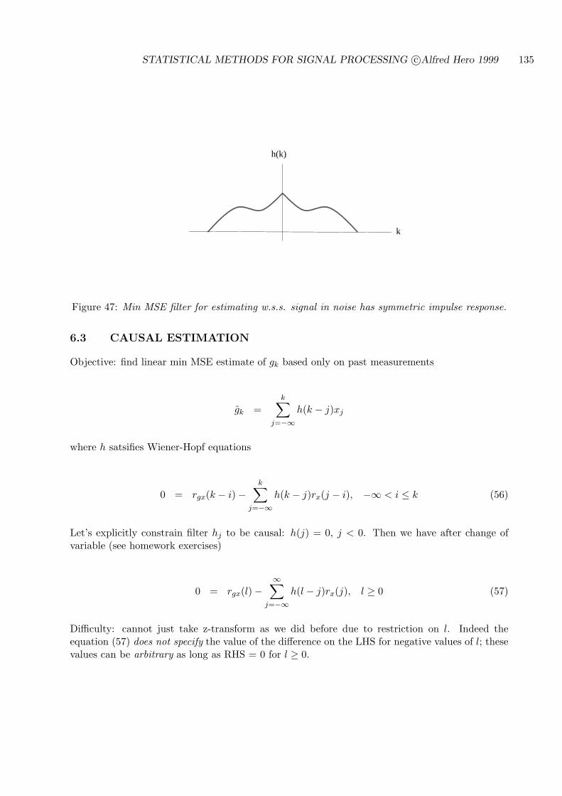
STATISTICAL METHODS FOR SIGNAL PROCESSING c©Alfred Hero 1999 135
h(k)
k
Figure 47: Min MSE filter for estimating w.s.s. signal in noise has symmetric impulse response.
6.3 CAUSAL ESTIMATION
Objective: find linear min MSE estimate of gk based only on past measurements
gk =k∑
j=−∞h(k − j)xj
where h satsifies Wiener-Hopf equations
0 = rgx(k − i)−k∑
j=−∞h(k − j)rx(j − i), −∞ < i ≤ k (56)
Let’s explicitly constrain filter hj to be causal: h(j) = 0, j < 0. Then we have after change ofvariable (see homework exercises)
0 = rgx(l)−∞∑
j=−∞h(l − j)rx(j), l ≥ 0 (57)
Difficulty: cannot just take z-transform as we did before due to restriction on l. Indeed theequation (57) does not specify the value of the difference on the LHS for negative values of l; thesevalues can be arbitrary as long as RHS = 0 for l ≥ 0.
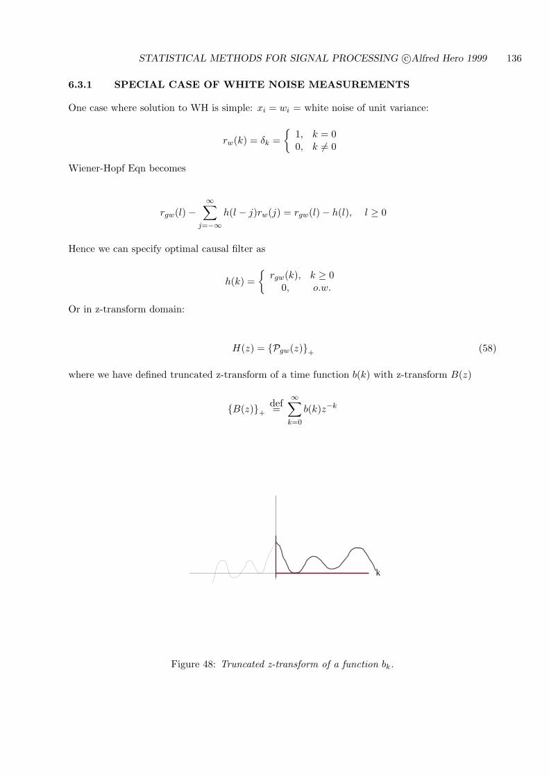
STATISTICAL METHODS FOR SIGNAL PROCESSING c©Alfred Hero 1999 136
6.3.1 SPECIAL CASE OF WHITE NOISE MEASUREMENTS
One case where solution to WH is simple: xi = wi = white noise of unit variance:
rw(k) = δk =
1, k = 00, k 6= 0
Wiener-Hopf Eqn becomes
rgw(l)−∞∑
j=−∞h(l − j)rw(j) = rgw(l)− h(l), l ≥ 0
Hence we can specify optimal causal filter as
h(k) =
rgw(k), k ≥ 00, o.w.
Or in z-transform domain:
H(z) = Pgw(z)+ (58)
where we have defined truncated z-transform of a time function b(k) with z-transform B(z)
B(z)+def=
∞∑
k=0
b(k)z−k
k
Figure 48: Truncated z-transform of a function bk.
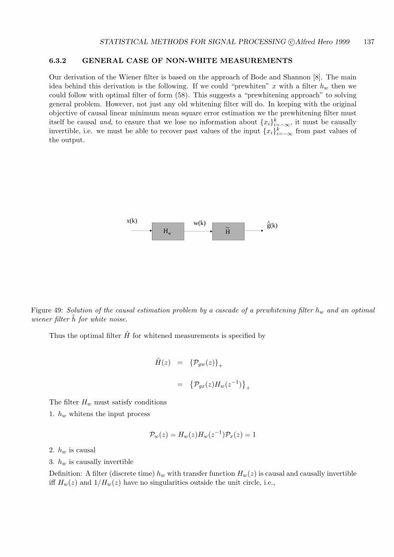
STATISTICAL METHODS FOR SIGNAL PROCESSING c©Alfred Hero 1999 137
6.3.2 GENERAL CASE OF NON-WHITE MEASUREMENTS
Our derivation of the Wiener filter is based on the approach of Bode and Shannon [8]. The mainidea behind this derivation is the following. If we could “prewhiten” x with a filter hw then wecould follow with optimal filter of form (58). This suggests a “prewhitening approach” to solvinggeneral problem. However, not just any old whitening filter will do. In keeping with the originalobjective of causal linear minimum mean square error estimation we the prewhitening filter mustitself be causal and, to ensure that we lose no information about xik
i=−∞, it must be causallyinvertible, i.e. we must be able to recover past values of the input xik
i=−∞ from past values ofthe output.
x(k) w(k) g(k)^Hw H
~
Figure 49: Solution of the causal estimation problem by a cascade of a prewhitening filter hw and an optimalwiener filter h for white noise.
Thus the optimal filter H for whitened measurements is specified by
H(z) = Pgw(z)+
=Pgx(z)Hw(z−1)
+
The filter Hw must satisfy conditions
1. hw whitens the input process
Pw(z) = Hw(z)Hw(z−1)Px(z) = 1
2. hw is causal
3. hw is causally invertible
Definition: A filter (discrete time) hw with transfer function Hw(z) is causal and causally invertibleiff Hw(z) and 1/Hw(z) have no singularities outside the unit circle, i.e.,
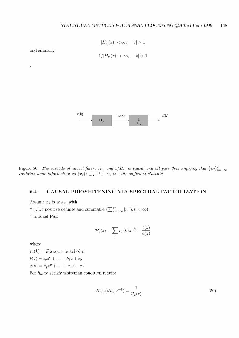
STATISTICAL METHODS FOR SIGNAL PROCESSING c©Alfred Hero 1999 138
|Hw(z)| < ∞, |z| > 1
and similarly,1/|Hw(z)| < ∞, |z| > 1
.
x(k) w(k)Hw Hw
1 x(k)
Figure 50: The cascade of causal filters Hw and 1/Hw is causal and all pass thus implying that wiki=−∞
contains same information as xiki=−∞, i.e. wi is white sufficient statistic.
6.4 CAUSAL PREWHITENING VIA SPECTRAL FACTORIZATION
Assume xk is w.s.s. with
* rx(k) positive definite and summable(∑∞
k=−∞ |rx(k)| < ∞)
* rational PSD
Px(z) =∑
k
rx(k)z−k =b(z)a(z)
where
rx(k) = E[xixi−k] is acf of x
b(z) = bqzq + · · ·+ b1z + b0
a(z) = apzp + · · ·+ a1z + a0
For hw to satisfy whitening condition require
Hw(z)Hw(z−1) =1
Px(z)(59)
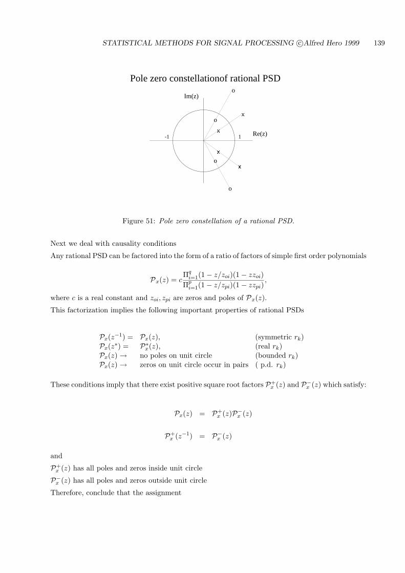
STATISTICAL METHODS FOR SIGNAL PROCESSING c©Alfred Hero 1999 139
Pole zero constellationof rational PSD
Re(z)
Im(z)
o
o
o
o
1-1
Figure 51: Pole zero constellation of a rational PSD.
Next we deal with causality conditions
Any rational PSD can be factored into the form of a ratio of factors of simple first order polynomials
Px(z) = cΠq
i=1(1− z/zoi)(1− zzoi)Πp
i=1(1− z/zpi)(1− zzpi),
where c is a real constant and zoi, zpi are zeros and poles of Px(z).
This factorization implies the following important properties of rational PSDs
Px(z−1) = Px(z), (symmetric rk)Px(z∗) = P∗x(z), (real rk)Px(z) → no poles on unit circle (bounded rk)Px(z) → zeros on unit circle occur in pairs ( p.d. rk)
These conditions imply that there exist positive square root factors P+x (z) and P−x (z) which satisfy:
Px(z) = P+x (z)P−x (z)
P+x (z−1) = P−x (z)
and
P+x (z) has all poles and zeros inside unit circle
P−x (z) has all poles and zeros outside unit circle
Therefore, conclude that the assignment
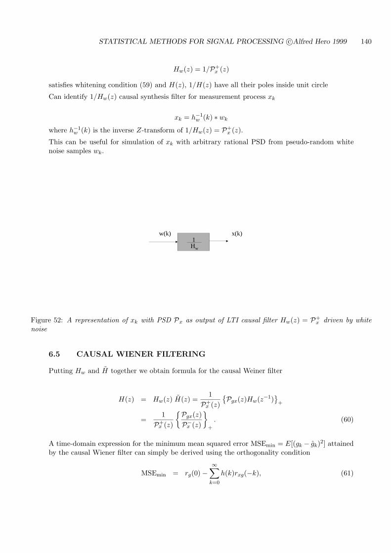
STATISTICAL METHODS FOR SIGNAL PROCESSING c©Alfred Hero 1999 140
Hw(z) = 1/P+x (z)
satisfies whitening condition (59) and H(z), 1/H(z) have all their poles inside unit circle
Can identify 1/Hw(z) causal synthesis filter for measurement process xk
xk = h−1w (k) ∗ wk
where h−1w (k) is the inverse Z-transform of 1/Hw(z) = P+
x (z).
This can be useful for simulation of xk with arbitrary rational PSD from pseudo-random whitenoise samples wk.
w(k)
Hw
1 x(k)
Figure 52: A representation of xk with PSD Px as output of LTI causal filter Hw(z) = P+x driven by white
noise
6.5 CAUSAL WIENER FILTERING
Putting Hw and H together we obtain formula for the causal Weiner filter
H(z) = Hw(z) H(z) =1
P+x (z)
Pgx(z)Hw(z−1)
+
=1
P+x (z)
Pgx(z)P−x (z)
+
. (60)
A time-domain expression for the minimum mean squared error MSEmin = E[(gk − gk)2] attainedby the causal Wiener filter can simply be derived using the orthogonality condition
MSEmin = rg(0)−∞∑
k=0
h(k)rxg(−k), (61)
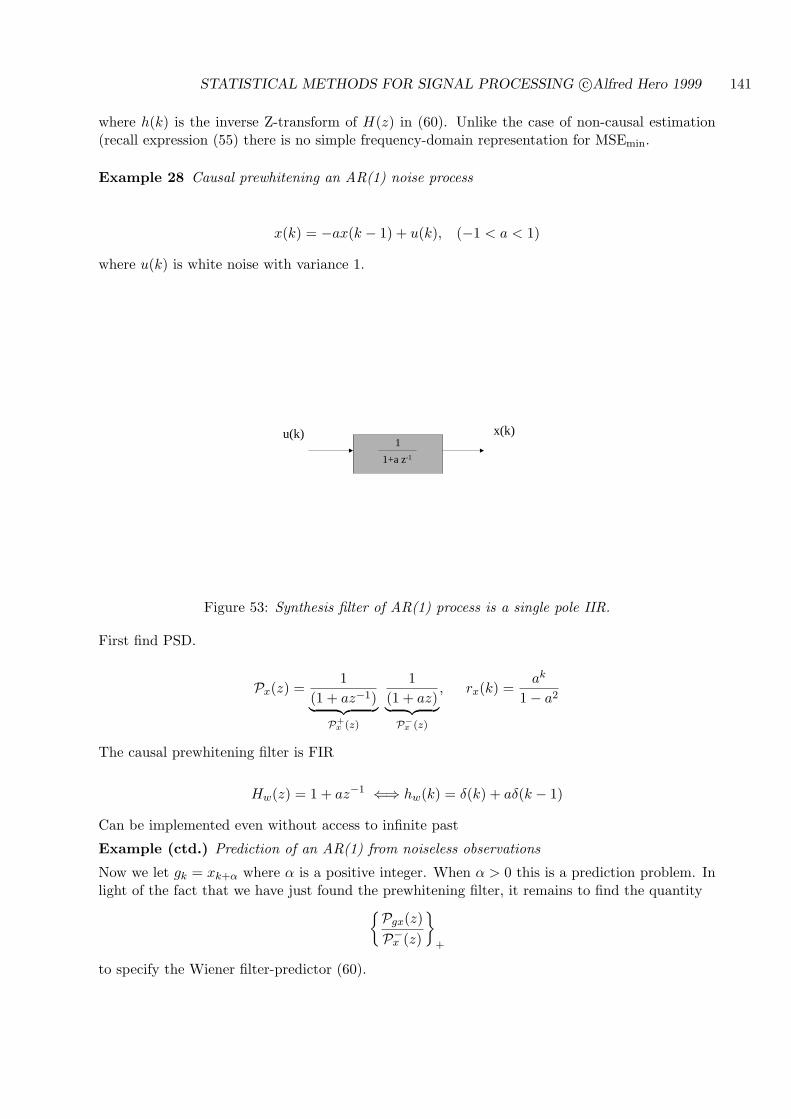
STATISTICAL METHODS FOR SIGNAL PROCESSING c©Alfred Hero 1999 141
where h(k) is the inverse Z-transform of H(z) in (60). Unlike the case of non-causal estimation(recall expression (55) there is no simple frequency-domain representation for MSEmin.
Example 28 Causal prewhitening an AR(1) noise process
x(k) = −ax(k − 1) + u(k), (−1 < a < 1)
where u(k) is white noise with variance 1.
u(k) x(k)
1+a z-1
1
Figure 53: Synthesis filter of AR(1) process is a single pole IIR.
First find PSD.
Px(z) =1
(1 + az−1)︸ ︷︷ ︸P+
x (z)
1(1 + az)︸ ︷︷ ︸P−x (z)
, rx(k) =ak
1− a2
The causal prewhitening filter is FIR
Hw(z) = 1 + az−1 ⇐⇒ hw(k) = δ(k) + aδ(k − 1)
Can be implemented even without access to infinite past
Example (ctd.) Prediction of an AR(1) from noiseless observations
Now we let gk = xk+α where α is a positive integer. When α > 0 this is a prediction problem. Inlight of the fact that we have just found the prewhitening filter, it remains to find the quantity
Pgx(z)P−x (z)
+
to specify the Wiener filter-predictor (60).
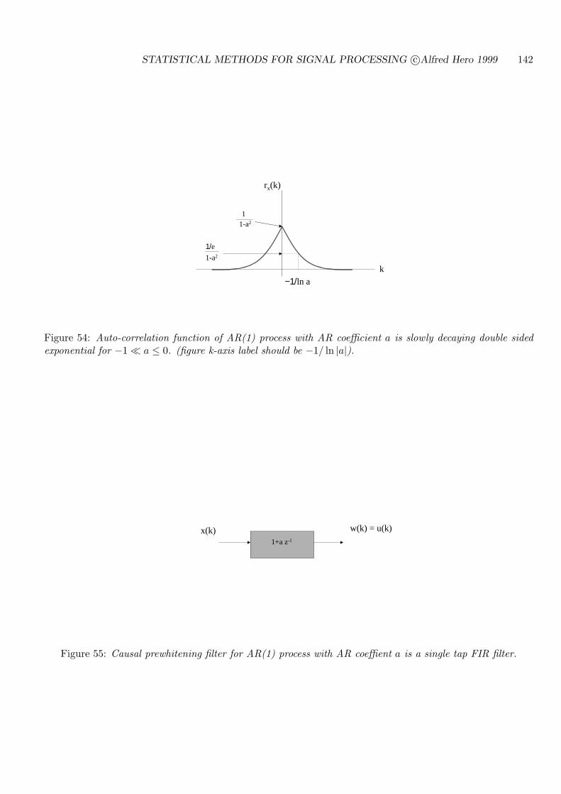
STATISTICAL METHODS FOR SIGNAL PROCESSING c©Alfred Hero 1999 142
rx(k)
1-a2
1
k−1/ln a
1/e1-a2
Figure 54: Auto-correlation function of AR(1) process with AR coefficient a is slowly decaying double sidedexponential for −1 ¿ a ≤ 0. (figure k-axis label should be −1/ ln |a|).
x(k) w(k) = u(k)
1+a z-1
Figure 55: Causal prewhitening filter for AR(1) process with AR coeffient a is a single tap FIR filter.
STATISTICAL METHODS FOR SIGNAL PROCESSING c©Alfred Hero 1999 143
As rgx(k) = E[xi+αxi−k] = rx(k + α): Pgx(z) = zαPx(z). HencePgx(z)P−x (z)
+
=zαP+
x (z)
+
=zα/(1 + az−1)
+
Now, using the identity (81) derived in the exercises, we see thatzα/(1 + az−1)
+
= (−a)α/(1 + az−1)
Hence, the Wiener filter-predictor is simply
H(z) =1
P+x (z)
((−a)α
1 + az−1
)= (−a)α
which in the time domain gives the optimal predictor as xk+α = (−a)αxk. This just correspondsto scaling the most recent observation and is consistent with xk being a 1st order Markov sequenceso that, for predicting the future, past information is not useful given present information.
Example 29 Causally prewhitening an AR(1) plus white noise process
x(k) = vAR(1)(k) + V (k)
where
* vAR(1)(k) is AR(1) with a = −0.8
* V (k) is white noise of variance 1/0.36
* vAR(1)(k) and V (k) are uncorrelated
Using result (80) derived in the Exercises, find PSD as a rational function with double pole anddouble zero
Px(z) =1
(1− 0.8z−1)1
(1− 0.8z)+ 1/0.36
=d(1 + bz−1)(1 + az−1)︸ ︷︷ ︸
P+x (z)
d(1 + bz)(1 + az)︸ ︷︷ ︸P−x (z)
where a = −0.8, b = −0.5 and d = 1/√
0.225.
Unlike previous example, the causal prewhitening filter hw(k) is now IIR
Hw(z) = 1/d(1 + az−1)(1 + bz−1)
and thus prewhitening cannot be implemented without access to infinite past.
STATISTICAL METHODS FOR SIGNAL PROCESSING c©Alfred Hero 1999 144
Note that the synthesis filter 1/Hw(z) can be applied to white noise wk to obtain recursion forxk with both an autoregressive (AR) component (LHS) and a moving average (MA) component(RHS):
xk + axk−1 = b1wk + b2wk−1
where b1 = d and b2 = db. Random processes xk that satisfy the recursion above are “ARMA(1,1)”process.
Example (ctd.) Prediction of AR(1) from noisy observations
Similarly to the previous example we let g(k) = vAR(1)(k+α) where α is a non-negative integer. Asthe measurement noise u(k) and the AR(1) process vAR(1)(k) are uncorrelated Pgx(z) = Pgv(z) =zαPv(z) where Pv(z) is the PSD of vAR(1) and Pgv(z) is the cross spectral density of g and vAR(1).Therefore, after substitution of the expression for P−x obtained above,
Pgx(z)P−x (z)
+
=1d
zα 1
1 + bz
11 + az−1
+
. (62)
Before proceeding further, we will need to express the product of two ratios in ·+ as a sum oftwo ratios in order to apply the identities (81) and (82). To do this, observe
11 + bz
11 + az−1
=z−1
b + z−1
11 + az−1
=A
b + z−1+
B
1 + az−1
where A and B are to be determined. Comparing the LHS of the top line to the bottom line ofthis last equation it is obvious that
A = limz−1→−b
z−1
1 + az−1= −b/(1− ab)
B = limz−1→−1/a
z−1
b + z−1= 1/(1− ab)
Thus we have from (62)Pgx(z)P−x (z)
+
=1
d(1− ab)
zα
1 + az−1− zα+1b
1 + bz
+
=1
d(1− ab)(−a)α
1 + az−1
where we have used the identity (82) which shows that only the first additive term in ·+ survives(the second term corresponds to an anticausal component).
Hence, using (60) the Wiener filter-predictor is simply
H(z) =q
1 + bz−1
where q = (−a)α
d2(1−ab), which can be implemented in the time domain as the single pole IIR filter
recursiong(k) = −bg(k − 1) + qxk.
STATISTICAL METHODS FOR SIGNAL PROCESSING c©Alfred Hero 1999 145
with g(k) = vAR(1)(k + α). It can be readily verified that in the limit as the measurement noisevar(u(k)) goes to zero, b → 0, d2 → 1, and q → (−a)α so that this IIR predictor filter reduces tothe simple Wiener predictor filter of the previous example having no measurement noise.
Derivation of the MSE of the Wiener filter is left as an exercise for the reader.
6.6 CAUSAL FINITE MEMORY TIME VARYING ESTIMATION
The Wiener filter is limited to the cases where the processes gk and xk are jointly w.s.s. and theestimating filter is LTI, i.e. access to infinite past is available. In practice, however, this is not thecase and we will need to handle the situation for which
1. gk, xk may not be jointly w.s.s.
2. estimator filter is turned on at time k = 0 with initial conditions (finite memory) and is notLTI.
Objective: find linear min MSE estimate of gk based only on finite past+present measurements
gk =k∑
j=0
h(k, j)xj (63)
We know that optimal h satisfies the k × k system of Wiener-Hopf equations.
0 = rgx(k, i)−k∑
j=0
h(k, j)rx(j, i), 0 ≤ i ≤ k
Or, since summation is over finite number of indices we can express this in the familiar matrixform
hk = R−1x rxg
where hk = [h(k, k), h(k, k− 1), . . . , h(k, 1)]T , Rx is the (k + 1)× (k + 1) covariance matrix of thefirst k measurements, and rgx is the (k + 1)-element vector of cross correlations between g andx(0), . . . , x(k).
Difficulty: standard matrix inverse approach has growing memory and computation as k increases:not suitable for real time implementation.
6.6.1 SPECIAL CASE OF UNCORRELATED MEASUREMENTS
As before we first convert to a case where solution to WH is simple:
⇒ xi = ηi = non-stationary white noise
rη(j, i) = σ2η(i) δj−i
Solution to WH equation is now immediate
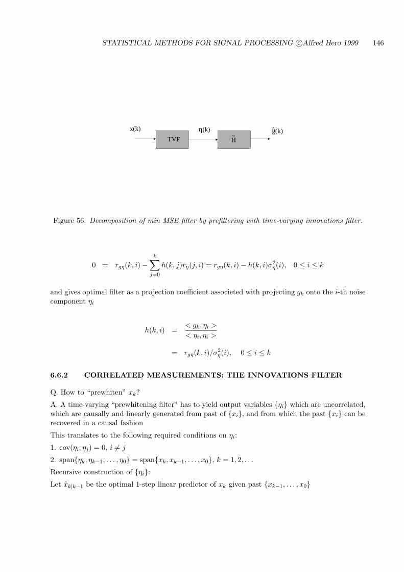
STATISTICAL METHODS FOR SIGNAL PROCESSING c©Alfred Hero 1999 146
x(k) η(k)
TVFg(k)
H~
^
Figure 56: Decomposition of min MSE filter by prefiltering with time-varying innovations filter.
0 = rgη(k, i)−k∑
j=0
h(k, j)rη(j, i) = rgη(k, i)− h(k, i)σ2η(i), 0 ≤ i ≤ k
and gives optimal filter as a projection coefficient associeted with projecting gk onto the i-th noisecomponent ηi
h(k, i) =< gk, ηi >
< ηi, ηi >
= rgη(k, i)/σ2η(i), 0 ≤ i ≤ k
6.6.2 CORRELATED MEASUREMENTS: THE INNOVATIONS FILTER
Q. How to “prewhiten” xk?
A. A time-varying “prewhitening filter” has to yield output variables ηi which are uncorrelated,which are causally and linearly generated from past of xi, and from which the past xi can berecovered in a causal fashion
This translates to the following required conditions on ηi:
1. cov(ηi, ηj) = 0, i 6= j
2. spanηk, ηk−1, . . . , η0 = spanxk, xk−1, . . . , x0, k = 1, 2, . . .
Recursive construction of ηi:Let xk|k−1 be the optimal 1-step linear predictor of xk given past xk−1, . . . , x0

STATISTICAL METHODS FOR SIGNAL PROCESSING c©Alfred Hero 1999 147
xk|k−1 =k−1∑
i=0
ak,i xi
Equivalently,
xk|k−1 =k−1∑
i=0
αk,i ηi
Recall orthogonality condition
E[(xk − xk|k−1)xi] = 0, i = 0, . . . , k − 1
Suggests following algorithm for ηi’s
η0 = x0
η1 = x1 − x1|0...
...ηk = xk − xk|k−1
or, more explicitly, in matrix form
η0...
ηk
=
1 0 · · · 0
−a10. . . 0
......
. . . . . . 0−ak,0 · · · −ak,k−1 1
x0...
xk
ηk
= A xk
* ηi is the ”innovations process”
* Rows of A specify causal invertible “innovations filter”
* Note: as A is invertible ηi is equivalent to xi.
6.6.3 INNOVATIONS AND CHOLESKY DECOMPOSITION
The innovations representation gives a decomposition for covariance Rx of x
Rx = E[xxT ]= E[A−1ηηTA−T ]
= A−1E[ηηT ]A−T
= A−1 Rη A−T
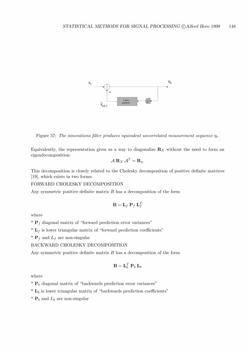
STATISTICAL METHODS FOR SIGNAL PROCESSING c©Alfred Hero 1999 148
Linearpredictor z-1
xk|k-1^
xkηk
-
Figure 57: The innovations filter produces equivalent uncorrelated measurement sequence ηi.
Equivalently, the representation gives us a way to diagonalize RX without the need to form aneigendecomposition:
A RX AT = Rη.
This decomposition is closely related to the Cholesky decomposition of positive definite matrices[19], which exists in two forms:
FORWARD CHOLESKY DECOMPOSITION
Any symmetric positive definite matrix B has a decomposition of the form
B = Lf Pf LTf
where
* Pf diagonal matrix of “forward prediction error variances”
* Lf is lower triangular matrix of “forward prediction coefficients”
* Pf and Lf are non-singular
BACKWARD CHOLESKY DECOMPOSITION
Any symmetric positive definite matrix B has a decomposition of the form
B = LTb Pb Lb
where
* Pb diagonal matrix of “backwards prediction error variances”
* Lb is lower triangular matrix of “backwards prediction coefficients”
* Pb and Lb are non-singular
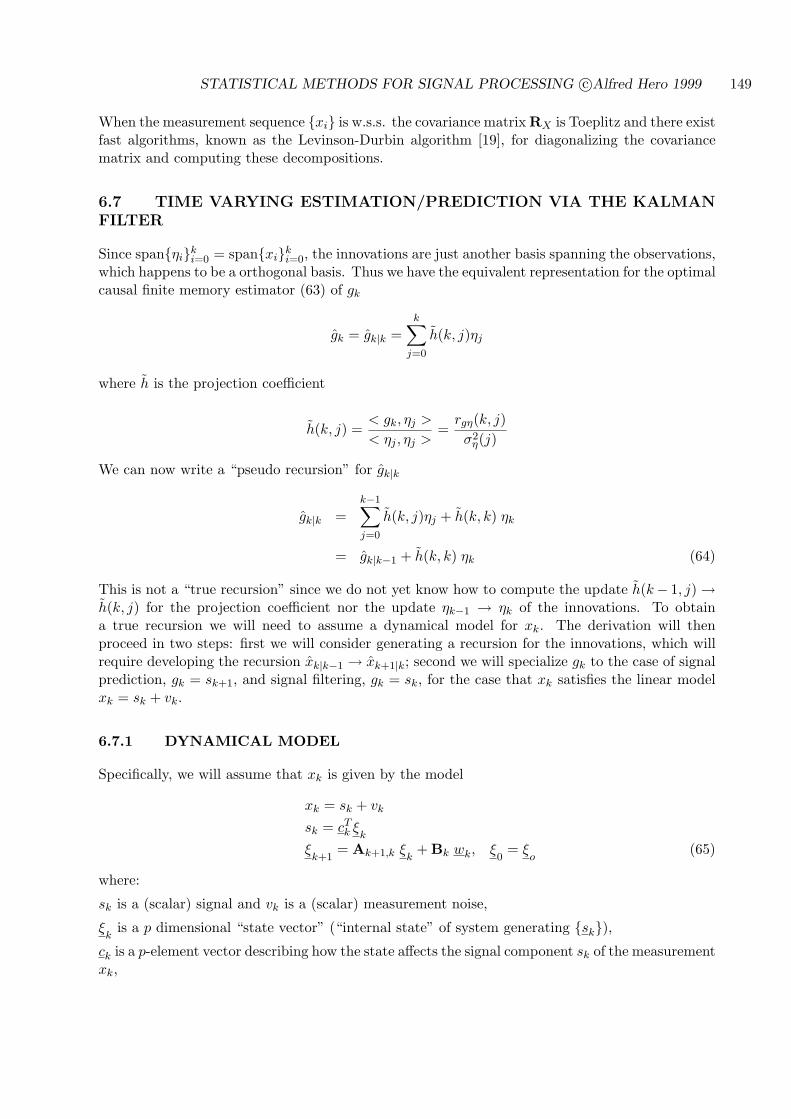
STATISTICAL METHODS FOR SIGNAL PROCESSING c©Alfred Hero 1999 149
When the measurement sequence xi is w.s.s. the covariance matrix RX is Toeplitz and there existfast algorithms, known as the Levinson-Durbin algorithm [19], for diagonalizing the covariancematrix and computing these decompositions.
6.7 TIME VARYING ESTIMATION/PREDICTION VIA THE KALMANFILTER
Since spanηiki=0 = spanxik
i=0, the innovations are just another basis spanning the observations,which happens to be a orthogonal basis. Thus we have the equivalent representation for the optimalcausal finite memory estimator (63) of gk
gk = gk|k =k∑
j=0
h(k, j)ηj
where h is the projection coefficient
h(k, j) =< gk, ηj >
< ηj , ηj >=
rgη(k, j)σ2
η(j)
We can now write a “pseudo recursion” for gk|k
gk|k =k−1∑
j=0
h(k, j)ηj + h(k, k) ηk
= gk|k−1 + h(k, k) ηk (64)
This is not a “true recursion” since we do not yet know how to compute the update h(k− 1, j) →h(k, j) for the projection coefficient nor the update ηk−1 → ηk of the innovations. To obtaina true recursion we will need to assume a dynamical model for xk. The derivation will thenproceed in two steps: first we will consider generating a recursion for the innovations, which willrequire developing the recursion xk|k−1 → xk+1|k; second we will specialize gk to the case of signalprediction, gk = sk+1, and signal filtering, gk = sk, for the case that xk satisfies the linear modelxk = sk + vk.
6.7.1 DYNAMICAL MODEL
Specifically, we will assume that xk is given by the model
xk = sk + vk
sk = cTk ξ
k
ξk+1
= Ak+1,k ξk
+ Bk wk, ξ0
= ξo
(65)
where:
sk is a (scalar) signal and vk is a (scalar) measurement noise,
ξk
is a p dimensional “state vector” (“internal state” of system generating sk),ck is a p-element vector describing how the state affects the signal component sk of the measurementxk,

STATISTICAL METHODS FOR SIGNAL PROCESSING c©Alfred Hero 1999 150
wk is a state noise vector (q × 1)
Bk is the state noise input matrix (p× q)
Ak+1,k is a state transition matrix (p× p) describing the signal dynamics which are due soley tothe initial condition ξ
o(in the absence of driving noise wk).
We make the following simplifying statistical assumptions:
State Model (SM) Assumptions A1-A4
A1 vk: uncorrelated sequence with zero mean and variance E[v2k] = σ2
v(k)
A2 wk: uncorrelated sequence with zero mean and covariance matrix E[wkwTk ] = Rw(k) (q × q)
A3 ξo
has zero mean and covariance matrix E[ξoξTo] = Rξ(0) (p× p)
A4 vk, ξ0, wj are mutually uncorrelated for all j, k
x(k)
v(k)
w(k)Bk
Ak+1|k
Ckz-1ξκ
ξκ+1s(k)
Figure 58: State space model for observation.
6.7.2 KALMAN RECURSIONS FOR INNOVATIONS AND STATE PREDIC-TION
For convenience, here we summarize the results derived in the next subsection. Under the as-sumptions A1-A4 the innovations ηk from xjk−1
j=0 can be recursively generated from the followingKalman recursions for innovation
Kalman Recursions for innovations and state prediction
First we have the Measurement Update Equations:
ηk = xk − cTk ξ
k|k−1(66)
ξk+1|k = Ak+1,k ξ
k|k−1+ Γk+1,k ηk, ξ
0|−1= 0 (67)
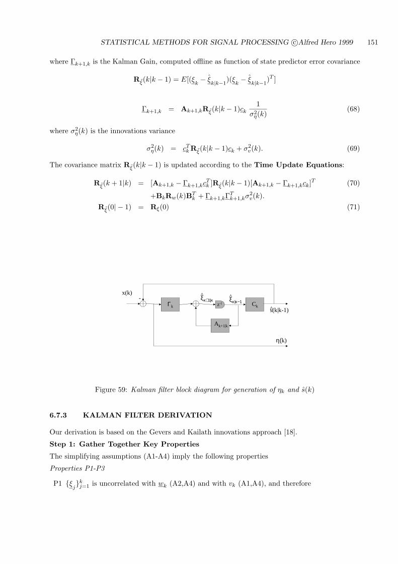
STATISTICAL METHODS FOR SIGNAL PROCESSING c©Alfred Hero 1999 151
where Γk+1,k is the Kalman Gain, computed offline as function of state predictor error covariance
Rξ(k|k − 1) = E[(ξk− ξ
k|k−1)(ξ
k− ξ
k|k−1)T ]
Γk+1,k = Ak+1,kRξ(k|k − 1)ck
1σ2
η(k)(68)
where σ2η(k) is the innovations variance
σ2η(k) = cT
k Rξ(k|k − 1)ck + σ2v(k). (69)
The covariance matrix Rξ(k|k − 1) is updated according to the Time Update Equations:
Rξ(k + 1|k) = [Ak+1,k − Γk+1,kcTk ]Rξ(k|k − 1)[Ak+1,k − Γk+1,kck]
T (70)
+BkRw(k)BTk + Γk+1,kΓ
Tk+1,kσ
2v(k).
Rξ(0| − 1) = Rξ(0) (71)
Γk
Ak+1|k
Ckz-1ξκ+1|κ
s(k|k-1)^
ξκ|κ−1^^x(k)
-
η(k)
Figure 59: Kalman filter block diagram for generation of ηk and s(k)
6.7.3 KALMAN FILTER DERIVATION
Our derivation is based on the Gevers and Kailath innovations approach [18].
Step 1: Gather Together Key Properties
The simplifying assumptions (A1-A4) imply the following properties
Properties P1-P3
P1 ξjk
j=1 is uncorrelated with wk (A2,A4) and with vk (A1,A4), and therefore
STATISTICAL METHODS FOR SIGNAL PROCESSING c©Alfred Hero 1999 152
P2 xjkj=1 is uncorrelated with wk and vk+1.
P3 < xk, ηj >=< sk + vk, ηj >=< sk, ηj >, j < k, since < vk, ηj >= 0, j < k, as ηj ∈spanxj , xj−1, . . . , x0 and vk is uncorrelated sequence (A1).
Step 2: establish relation between xk|k−1 and ξk|k−1
Putting P2 and P3 together we obtain from representation (64) for gk = sk:
xk|k−1 =k−1∑
j=0
< sk, ηj >
‖ηj‖2ηj
= cTk
k−1∑
j=0
< ξk, ηj >
‖ηj‖2ηj
︸ ︷︷ ︸ξ
k|k−1
.
Step 3: Establish update formula for ξk|k−1
→ ξk+1|k
Recall that the linear minimum mean square estimator for a random vector is simply the con-catenation of the linear minimum mean square estimators for each element of the random vector.Thus, with abuse of notation, denoting < ξ
k+1, ηk > the vector composed of inner products
< (ξk+1)i, ηk >, i = 1, . . . , p,
ξk+1|k =
k∑
j=0
< ξk+1
, ηj >
‖ηj‖2ηj
=k−1∑
j=0
< ξk+1
, ηj >
‖ηj‖2ηj +
< ξk+1
, ηk >
‖ηk‖2ηk (72)
Define the Kalman gain vector
Γk+1,k =< ξ
k+1, ηk >
‖ηk‖2, (73)
and note that, from the state equation (65) for ξk
and the fact that wk and ηj are uncorrelatedfor j ≤ k,
< ξk+1
, ηj >
‖ηj‖2=
< Ak+1,kξk, ηj >
‖ηj‖2+
< Bkwk, ηj >
‖ηj‖2
= Ak+1,k
< ξk, ηj >
‖ηj‖2, j ≤ k
which is Ak+1,k times the projection coefficient for projecting ξk
onto ηj .
Substitution of the above back into (72) gives the desired recursion
ξk+1|k = Ak+1,k
k−1∑
j=0
< ξk, ηj >
‖ηj‖2ηj + Γk+1,kηk
= Ak+1,kξk|k−1+ Γk+1,kηk (74)
STATISTICAL METHODS FOR SIGNAL PROCESSING c©Alfred Hero 1999 153
with initial condition ξ0|−1
= 0.
Step 4: Find expression for ‖ηk‖2
Define the state estimator error vector
ξk|k−1
= ξk− ξ
k|k−1.
Then, again using the state model for xk,
ηk = xk − xk|k−1 = cTk ξ
k+ vk − cT
k ξk|k−1
= cTk ξ
k|k−1+ vk (75)
We can use this result to find the innovations variance ‖ηk‖2 = σ2η(k) which is required for com-
puting the projection coefficients in (72), specifically the Kalman gain (73) needed for recursion(74). As ξ
k|k−1∈ spanξk, xk−1, . . . , x0, ξ
k|k−1is uncorrelated with vk, from (75)
σ2η(k) = cT
k Rξ(k|k − 1)ck + σ2v(k) (76)
where Rξ(k|k − 1) is the state estimator error covariance matrix. To evaluate this we will needto establish a recursion for this error covariance matrix. However, an expression for the Kalmangain will be required to develop the error covariance update equations.
Step 5: Express Kalman gain Γk+1,k in terms of state estimator error covarianceRξ(k|k − 1)
The Kalman gain vector Γk+1,k (73) can be related to the state estimator error covariance by thefollowing steps
1. < ξk+1
, ηk >= Ak+1,k < ξk, ηk > +Bk < wk, ηk >= Ak+1,k < ξ
k, ηk > (from whiteness of wk
and fact that ηk ∈ spanxk, . . . , x0).2. < ξ
k, ηk >=< ξ
k− ξ
k|k−1, ηk >=< ξ
k|k−1, ηk > (noting that < ξ
k|k−1, ηk >= 0 from orthogo-
nality principle of linear estimation)
3. < ξk|k−1
, ηk >= E[ξk|k−1
ηk] = E[ξk|k−1
ξT
k|k−1]ck (ηk = cT
k ξk|k−1
+ vk and vk is white noise
uncorrelated with ξk|k−1
)
Putting the above together, and recalling that ‖ηk‖2 = σ2η(k) calculated in (76), we obtain
Γk+1,k =< ξ
k+1, ηk >
‖ηk‖2= Ak+1,k
< ξk, ηk >
‖ηk‖2
= Ak+1,kRξ(k|k − 1)ck
1cTk Rξ(k|k − 1)ck + σ2
v(k)(77)
Step 6: Find recursive update for estimator error covariance Rξ(k|k−1) → Rξ(k+1|k)
First find update equation for ξk|k−1
by subtracting the state estimator update equation (74) fromthe actual state update equation (65)
ξk+1
− ξk+1|k = Ak+1,k(ξk
− ξk|k−1
) + Bkwk − Γk+1,kηk.
STATISTICAL METHODS FOR SIGNAL PROCESSING c©Alfred Hero 1999 154
Identifying ξk+1|k = ξ
k+1− ξ
k+1|k and using ηk = cTk ξ
k|k−1+ vk in the above
ξk+1|k = Ak+1,kξk|k−1
+ Bkwk − Γk+1,k(cTk ξ
k|k−1+ vk)
= [Ak+1,k − Γk+1,kcTk ]ξ
k|k−1+ Bkwk − Γk+1,kvk (78)
Now properties P1-P3 imply that the three additive terms in (78) are mutually uncorrelated.Therefore, the covariance of the RHS is the sum of three covariance matrices and we obtain theupdate equation (71)
Rξ(k + 1|k) = [Ak+1,k − Γk+1,kcTk ]Rξ(k|k − 1)[Ak+1,k − Γk+1,kc
Tk ]T
+BkRw(k)BTk + Γk+1,kΓ
Tk+1,kσ
2v(k).
An alternative form of the recursion (71) can be derived by using (69) and (73) which makesRξ(k|k − 1) explicit in the quantity Γk+1,k. After some algebra this produces the equivalentupdate equation
Rξ(k + 1|k) = Ak+1,kRξ(k|k − 1)ATk+1,k + BkRw(k)BT
k
−Ak+1,kRξ(k|k − 1)cTk ckRξ(k|k − 1)AT
k+1,k/σ2η(k) (79)
where σ2η(k) = cT
k Rξ(k|k − 1)ck + σ2v(k), as defined above.
6.8 KALMAN FILTERING: SPECIAL CASES
The Kalman filter equation (67) generates the innovations sequence ηk which is needeed to com-pute the estimate gk|k defined in Sec. 6.7 by the equation (64). Also needed are the projectioncoefficients h(k, j), j = 1, . . . , k. We discuss two special cases for which these coefficients aresimply computed, Kalman prediction and Kalman filtering
6.8.1 KALMAN PREDICTION
The linear prediction problem is to predict future value of the observation xk+1 from a linearcombination of past and present observations xjk
j=0, or, equivalently, from the past and presentinnovations ηjk
j=0. Recalling the measurement model (65), xk+1 = sk+1 +vk+1 is the sum of twouncorrelated components. Hence, denoting the predictor by xk+1|k and applying the superpositionproperty (52) of linear estimators of a sum of random variables
xk+1|k = sk+1|k + vk+1|k = sk+1|k
where vk+1|k = 0 due to the fact that vk is white and thus uncorrelated with the past innovations,i.e. unpredictable. Finally, as sk+1 = cT
k+1ξk+1
sk+1|k = cTk+1ξk+1|k
which can be computed from the Kalman filter (67) for state estimation discussed in the previoussub-section.

STATISTICAL METHODS FOR SIGNAL PROCESSING c©Alfred Hero 1999 155
6.8.2 KALMAN FILTERING
The filtering problem is to estimate the signal component sk in xk = sk +vk from past and presentmeasurements xjk
j=0 (equivalently ηjkj=0). Let sk|k denote this estimate. Set gk = sk and from
the general recursion (64) we obtain
sk|k = sk|k−1 + h(k, k)ηk,
where sk|k−1 is the linear predictor derived in the last subsection and
h(k, k) =E[skηk]var(ηk)
=cTk E[ξ
kηk]
var(ηk).
Recall that in the process of showing the expression (77) for the Kalman gain Γk+1,k we establishedE[ξ
kηk] = Rξ(k|k − 1)ck. Putting this together with the expression (69) we obtain
h(k, k) =cTk Rξ(k|k − 1)ck
cTk Rξ(k|k − 1)ck + σ2
v(k).
All of the above quantites are available from the Kalman filter recursions (66) and (71).
6.9 KALMAN FILTER FOR SPECIAL CASE OF GAUSSIAN STATE ANDNOISE
Assume:
* vk, ξo
and wk are jointly Gaussian
Then:
* xk = sk + vk is a Gaussian random process
* Kalman filter yields min MSE state predictor
ξk|k−1
= E[ξk|xk−1, . . . , x1]
* ηk is an equivalent uncorrelated Gaussian measurement
6.10 STEADY STATE KALMAN FILTER AND WIENER FILTER
Assume
* Ak+1,k, bk, ck and Rw(k) are time-invariant
* Rv(k) is time-invariant
* The state error covariance matrix Rξ(k +1, k) converges to a positive definite matrix as k →∞.
Then:
* sk is w.s.s. as k →∞* xk is w.s.s. as k →∞⇒ Steady state innovations filter is equivalent to Wiener prewhitening filter
STATISTICAL METHODS FOR SIGNAL PROCESSING c©Alfred Hero 1999 156
In particular, in steady state, ηk becomes a (w.s.s.) white noise with
σ2η(k) → σ2
η(∞) = cTRξ(∞)c + σ2v
The steady state error covariance matrix Rξ(∞) can be found in two steps:
Step 1: set Rξ(k, k−1) = Rξ(k+1, k) = Rξ(∞) in covariance update equation (71), equivalently,(79), obtaining the steady state covariance equation:
Rξ(∞) = ARξ(∞)AT + BRwBT
−ARξ(∞)cT cRξ(∞)AT /σ2η(∞),
Step 2: Noting that, as σ2η(∞) is linear in Rξ(∞), the steady state covariance equation is equiv-
alent to a quadratic equation in Rξ(∞), called an algebraic Ricatti equation [32]. This can besolved numerically but for small state dimension Rξ(∞) it can be often found by hand.
Example 30 Kalman filter for estimation of a constant signal
This example is credited to R. Raich. The objective is to find an optimal recursive estimator of aconstant signal in random noise given a finite number of observations. Accordingly, let’s assumethe following special case of the dynamical observation model (65)
xk = sk + vk
sk+1 = sk.
Here sk is a scalar state and we can identify ck = 1,Bk = 0,Ak+1,k = 1, and Rξ(0) = σ2s . For
notational simplicity define the normalized state error covariance (actually the variance since thestate is one dimensional):
Tk+1 = Rξ(k + 1, k)/σ2v .
With this notation, and the identifications above, the (scalar) update equation (79) for Rξ(k+1, k)gives
Tk+1 = Tk/(Tk + 1), To = σ2s/σ2
v ,
which has explicit solution Tk = 1/(k + 1/SNR), where SNR= σ2s/σ2
v . The Kalman gain is simply
Γk+1,k =Tk
Tk + 1= Tk+1.
Therefore, the Kalman filter update for sk|k−1 is
sk+1|k = sk|k−1 + Γk+1,kηk,
which, using ηk = xk − sk|k−1 is equivalent to the AR(1) recursion
sk+1|k = [1− Γk+1,k]sk|k−1 + Γk+1,kxk,
with initial condition s0|−1 = 0. approximation to Γk+1,k = Tk+1:
Tk+1 ≈ 1k + 1
,
STATISTICAL METHODS FOR SIGNAL PROCESSING c©Alfred Hero 1999 157
yielding the large k form of the AR(1) recursion:
sk+1|k =k
k + 1sk|k−1 +
1k + 1
xk,
which is equivalent to
sk+1|k =1
k + 1
k∑
i=0
xk.
Thus, as expected, the Kalman filter estimator of a constant signal becomes identical to the samplemean estimator of the ensemble mean for large k - as the transients of the filter die down the initialcondition has no more influence.
It should be observed in the above example that the Kalman filter does not converge in steadystate to a LTI filter since the asymptotic state covariance is not positive definite - the variance isequal to zero.
6.11 SUMMARY OF STATISTICAL PROPERTIES OF THE INNOVA-TIONS
We summarize important properties of the innovations that will be important in the sequel. Asthe observation noise vk is uncorrelated with the signal sk, we have three equivalent expressionsfor the innovations
ηk = xk − xk|k−1
ηk = xk − sk|k−1
ηk = cTk (ξ
k− ξ
k|k−1) + vk
Furthermore:
E[ηi] = 0cov(ηi, ηj) = 0, i 6= j
and, as shown above, the innovations variance is
var(ηk) = σ2η(k)
= cTk Rξ(k)ck + σ2
v(k)
6.12 BACKGROUND REFERENCES
The Wiener filter was originally published (as a classified report) by Norbert Wiener in the early1940’s and the Kalman filter was published by Kalman and Bucy in the early 1960’s. The bookby Kailath [32] provides a nice overview of the historical context for both of these breakthroughs.

STATISTICAL METHODS FOR SIGNAL PROCESSING c©Alfred Hero 1999 158
Other books covering linear prediction from a signal processing perspective are Hayes [23], Mendel[44], and Moon and Stirling [48]. A very comprehensive mathematically concise coverage of signalprocessing algorithms for non-statistical least squares and linear prediction can be found in thebook by Strobach [69]. Finally, for a different time series perspective of mathematical statisticsthe reader can consult the excellent book by Brockwell and Davis [12].
6.13 APPENDIX: POWER SPECTRAL DENSITIES
Here we provide a quick primer on autocorrelation functions (acf) and power spectral densities(PSD) for zero mean wide sense stationary (wss) random sequences. For more detailed informationsee Thomas [71] or Davenport and Root [13].
6.13.1 ACF AND CCF
The autocorrelation function of a zero mean finite variance discrete time random process xk isdefined as
rx(i, j) = E[xix∗j ].
The acf is non-negative definite in the sense that for any absolutely summable sequence uk∑
i,j
u∗i rx(i, j)uj ≥ 0.
For two zero mean finite variance discrete time random sequences xk and yk the cross-correlationfunction (ccf) of x and y is defined as
rxy(i, j) = E[xiy∗j ].
The ccf has conjugate symmetry, rxy(i, j) = r∗yx(j, i), and is equal to zero when x and y areuncorrelated random sequences.
6.13.2 REAL VALUED WIDE SENSE STATIONARY SEQUENCES
When xk is zero mean real and wss its acf satisfies (by definition of wss): rx(i, j) = rx(i − j, 0).The function rx(i, i− k) is usually denoted as rx(k) and it is conjugate symmetric
rx(−k) = rx(k)
and satisfies rx(0) ≥ rx(k) for all k. A real wss xk has a PSD defined as the Discrete Time FourierTransform (DTFT) of rx:
Px(ω) = Frx(k) =∞∑
k=−∞rx(k)e−jωk
from which rx can be recovered using the inverse DTFT:
rx(k) = F−1Px(ω) =12π
∫ π
πPx(ω)ejωk.
STATISTICAL METHODS FOR SIGNAL PROCESSING c©Alfred Hero 1999 159
Due to the real, symmetric, non-negative definiteness of rx its PSD is real, symmetric, and non-negative:
P∗x(ω) = Px(ω), Px(−ω) = Px(ω), Px(ω) ≥ 0.
For two zero mean real jointly wss random sequences xk and yk the ccf similarly satisfies: rxy(i, i−k) = rxy(k). The ccf also has a kind of symmetry property rxy(−k) = ryx(k). The cross PSD isdefined as the DTFT of rxy. It is neither real nor symmetric but inherits the following propertyfrom rxy
Pxy(−ω) = P∗xy(ω) = Pyx(ω).
When xk and yk are uncorrelated the CPSD is equal to zero and therefore if zk = xk + yk
Pz(ω) = Px(ω) + Py(ω).
Let hk be the impulse response of a stable linear time invariant (LTI) system and let H(ω) = F(hk)be its frequency-domain transfer function. If yk = hk ∗ xk is the output of this LTI system then
Py(ω) = |H(ω)|2Px(ω),
andPxy(ω) = H∗(ω)Px(ω), Pyx(ω) = H(ω)Px(ω).
6.13.3 Z-DOMAIN PSD AND CPSD
Analogously to the frequency domain PSD defined above, one can define the z-domain PSD by
Px(z) = Zrx(k) =∞∑
k=−∞rx(k)z−k
We have the obvious relation Px(ω) = Px(ejω). The z-domain CPSD is defined analogously:Pxy(z) = Zrxy(k). The z-domain PSD and CPSD inherit various properties from their frequency-domain versions. In particular, radial symmetry about the unit circle
Px(z−1) = Px(z), Pxy(z−1) = Pyx(z)
and conjugate symmetryPx(z∗) = P∗x(z).
Finally, when yk = hk ∗ xk is the output of an LTI system with z-domain transfer function H(z)then we have the analogous relations to before
Py(z) = H(z)H(z−1)Px(z),
andPxy(z) = H(z−1)Px(z), Pyx(z) = H(z)Px(z).
NB: When there is little danger of confusion, we usually drop the tilde notation when expressingz-domain PSDs or transfer functions

STATISTICAL METHODS FOR SIGNAL PROCESSING c©Alfred Hero 1999 160
6.14 EXERCISES
6.1 As we know, the optimal filter h(k, j) for estimating the sample g(k) of the process g(k)∞i=−∞from zero mean process x(i)∞i=−∞ satisfies the Wiener-Hopf equation
rgx(k, i)−∞∑
j=−∞h(k, j)rx(i, j) = 0, −∞ < i < ∞
Show that when g and x are jointly w.s.s. random processes, i.e. rx(i, j) = rx(i − j) andrgx(k, i) = rgx(k − i), h(k, j) can be assumed to be linear time invariant (LTI), i.e. h(k, j) =h(k− j) will satisfy the WH equation. Now show that the same holds for the causal optimalfilter h(k, j) which satisfies
rgx(k, i)−∞∑
j=−∞h(k, j)rx(i, j) = 0, −∞ < i ≤ k.
(Hint: Find Weiner-Hopf equations for estimating y(k + l) where l is an arbitrary time shift,make a change of index i and a change of variable j and show by comparison to the Weiner-Hopf equations for estimating y(k) that h(k, j) = h(k − j, 0)).
6.2 Derive the equation (57) for the Causal Wiener filter 0 = rgx(l) − ∑∞m=−∞ h(l − m)rx(m)
from the original equation (56) by making two changes of variable in sequence: reindex i byl = k − i and reindex j by m = k − j.
6.3 For constants a, c and the definitions q = 1 + c + ca2, r = ca, derive the following identity
1(1 + az−1)
1(1 + az)
+ c =d(1 + bz−1)(1 + az−1)
d(1 + bz)(1 + az)
(80)
where
b =q/r ±
√(q/r)2 − 42
, d2 = q/(1 + b2)
Observe that when c is positive real, one of the roots in the equation for b satisfies |b| ≤ 1while the other satisfies |b| ≥ 1.
6.4 In the development of the causal and non-causal Weiner estimators we have assumed that allprocesses were zero mean. Here we deal with the case of non-zero mean w.s.s. processes forwhich the affine Weiner estimator is appropriate.Assume the measurement process xkk and the target process gkk to be estimated arew.s.s. and have non-zero means E[xk] = µx(k) and E[gk] = µg(k).
(a) The affine non-causal Wiener estimator of gk is defined by the filter h(k, j) and sequenceof constants sk as
gk = ak +∞∑
j=−∞h(k, j)xj
where h(k, j) and ak are selected to minimize the mean square estimation error MSE(h, a) =E[(gk−gk)2]. Show that the optimal filter satisfies h(k, j) = h(k−j) where h(j) is the op-timal linear time invariant non-causal Weiner filter for estimating the zero mean processgk − µg(k) from the centered zero mean measurements xk − µx(k) and that the optimalsequence ak is µg(k) +
∑∞j=−∞ h(k − j)µx(j). Further show that the minimum MSE of
the affine non-causal Wiener estimator is functionally independent of the means µg andµx.
STATISTICAL METHODS FOR SIGNAL PROCESSING c©Alfred Hero 1999 161
(b) Repeat question (a) for the case of the causal affine Wiener estimator which satisfies theadditional restriction that h(k, j) = h(k − j) = 0, k < j.
6.5 You have the measurement modelxk = s2
k + wk
where wk is zero mean white noise of variance σ2 and sk is a w.s.s. zero mean Gaussianrandom sequence with acf rs(k) = ak/(1− a2), k ≥ 0. wk is independent of sk.
(a) Find the quantities E[s2i s
2i−k] and E[s2
i si−k] (Hint: use the property that for any zeromean jointly Gaussian r.v.s W,X, Y, Z: E[XY Z] = 0 and E[WXY Z] = E[WX]E[Y Z]+E[WZ]E[XY ] + E[WY ]E[XZ])
(b) Using the results of (a) find the optimal affine non-causal Wiener estimator for sk. Ex-plain your result.
(c) Using the results of (a) find the optimal affine non-causal Wiener estimator for s2k.
6.6 Assume the measurement modelxk = ask + vk
where sk and vk are zero mean jointly w.s.s. and uncorrelated, and a is a random variableindependent of sk having mean µa and variance σ2
a.
(a) Find the non-causal Weiner filter for estimating sk.(b) Find the MSE of the output of the non-causal Weiner filter. How does it behave as a
function of µa and σ2a?
(c) Find the causal Weiner filter for estimating sk. Specialize to the case where sk is an AR(1)process as in Example 29 with pole at −a and where vk is white noise with variance σ2.
6.7 For |a| < 1, use the geometric series formula∑∞
k=0 ckzk = 1/(1− cz), |cz| < 1 to derive thefollowing two results:
zl
1 + az−1
+
=
(−a)l 1
1+az−1 , l ≥ 0zl
1+az−1 , l < 0(81)
and
zl
1 + az
+
=
1, l = 00, l > 0
(82)
Now apply these results to compute the Z-domain quantity (for l ≥ 0)
zl
(1 + az−1)(1 + bz)
+
|a|, |b| < 1
.
6.8 Let the measurement model bexk = hk ∗ sk + vk
where sk and vk are zero mean jointly w.s.s. and uncorrelated, and hk is a causal and causallyinvertible filter with Z-transform H(z).
(a) Find the non-causal Weiner filter for estimating sk.(b) Find the causal Weiner filter for estimating sk.
STATISTICAL METHODS FOR SIGNAL PROCESSING c©Alfred Hero 1999 162
(c) Compare the results for (a) and (b) to the estimator h−1k ∗ sk where sk is the output of
the standard Weiner filter for estimating sk using the measurement model xk = sk + vk
and h−1k is the inverse Z-transform of 1/H(z).
6.9 Let the measurement model be as in Example 29
xk = sk + vk
where sk and vk are zero mean jointly w.s.s. and uncorrelated. It is desired to estimategk = hk ∗ sk where hk is the causal FIR filter with transfer function
H(z) = 1 + αz−1, α ∈ (−1, 1)
. Assume that α 6= a 6= b.
(a) Find the non-causal Weiner filter for estimating gk.(b) Find the causal Weiner filter for estimating gk.(c) Compare the results for (a) and (b) to the estimator gk = hk ∗ sk where sk is alterna-
tively the output of the standard non-causal and causal Weiner filters, respectively, forestimating sk.
6.10 The process sk is a zero mean AR(2) process following the recursion
sk = 0.8sk−1 − 0.15sk−2 + wk
where wk is zero mean white noise of variance 1.5 uncorrelated with sk−1, sk−2, . . .. Theobservation is
xk = sk + vk
where vk is zero mean white noise with variance 0.5 independent of sk.
(a) Express the AR(2) recursion in Z-transform domain as Zsk = H(z)Zwk and use theinput/output PSD relation Ps(z) = H(z)H(z−1)Pw(z) to determine the PSD Ps(z) ofsk.
(b) Find the non-causal Wiener filter for estimating sk.(c) Find the causal Wiener filter for estimating sk.
6.11 TBD
6.12 A common multipath model for a communications receiver is that the direct path signal plusan attenuated and delayed indirect path version of the signal are received in additive whitenoise:
xk = sk + bsk−1 + wk
The objective is to estimate the signal sk given a set of measurements xkk. In the followingassume that wk is zero mean white with variance σ2
w, sk is zero mean white with varianceσ2
s , b is a constant |b| < 1, and sk, wk are uncorrelated. You can assume that (σ2s(1 + b2) +
σ2w)/(σ2
sb) = 5/2 if that helps simplify your answers to the following.
(a) Find the power spectral density (PSD) Px(ejω) of xk, the cross PSD Psx(ejω) of sk andxk, and the spectral factorization of Px(z), z ∈ Cl .
(b) Find the optimal non-causal Wiener filter for estimating sk.(c) Find the optimal causal Wiener filter for estimating sk.
STATISTICAL METHODS FOR SIGNAL PROCESSING c©Alfred Hero 1999 163
6.13 In the derivation of the discrete time Kalman filter we assumed that the state noise wk wasuncorrelated with the measurement noise v(k). In this problem we generalize the Kalmanfilter to the case where E[wkv(l)] = Vwvδkl where δkl is the kronecker delta function. Derivethe Kalman filter equations.
6.14 The measurement equation is given by
xk = sk + vk
where sk satisfies the dynamic model (|a| < 1)
sk+1 = ask + wk, s0 = so
and vk, wk, so are uncorrelated, vk and wk are zero mean white noises with variances σ2v and
σ2w, respectively.
(a) Derive the Kalman filter equations.
(b) Derive the steady state state error covariance (variance) Rs(∞) def= limk→∞Rs(K|K−1)by setting Rs(k + 1|k) = Rs(k|k − 1) = Rs(∞) in the Kalman error covariance updateformula and solving explicitly for Rs(∞). Find the corresponding steady state Kalmangain.
(c) By taking the Z-transform of the steady state Kalman state recursion show that theKalman predictor sk+1|k is the output of a LTI with input xk.
(d) Compare the steady state Kalman predictor previously derived to the causal Wienerpredictor based on the infinite past.
6.15 Let the random sequence xk be zero mean and wide sense stationary of the form
xk = sk + vk
where sk is a signal with PSD Ps and vk is a white noise. You only get to measure the valueof xk for odd indices k = 2n − 1, n = −∞, . . . ,∞. The objective is to estimate sk at bothodd and even time instants k. Note that when vk = 0 the problem reduces to ”filling in” themissing (even) data points.(a) What is the system of Wiener-Hopf equations which must be satisfied by the optimal
linear filter for estimating sk from the measurements? Is the solution to this systemof equations time-invariant? If so find an expression for the optimal non-causal Wienerfilter transfer function H(z).
(b) Now assume that sk = ask−1 + wk−1 where |a| < 1 and wk is white noise independentof vk. Derive Kalman filter equations for recursively generating estimates s2n−1|2n−1 ands2n|2n−1 from the past measurements x2k−1n
k=1. Does the KF reduce to a linear timeinvariant filter as n →∞.
6.16 Derive the minimum mean square error expression (61) for the Wiener filter and use it tofind the MSE of the optimal predictors of Examples 28 and 29.
6.17 In the following three exercises you will explore the extended Kalman filter (EKF) for non-linear state dynamics. Similarly to Section 6.7.3 of the notes we assume that the observationsyk obey a dynamical model, except that here we assume that the state can evolve non-linearlyand that the additive noises are Gaussian:
yk = sk + vk
sk = cT ξk
, k = 0, 1, . . .
ξk+1
= g(ξk) + Bkwk

STATISTICAL METHODS FOR SIGNAL PROCESSING c©Alfred Hero 1999 164
where g is a possibly non-linear p-dimensional function of the p-dimensional state vector ξk,
vk and wk are mutually independent zero mean temporally uncorrelated (white) noises whichare Gaussian distributed with variance σ2
v and covariance matrix Rw, respectively. All otherassumptions on the model are identical to those made in Section 6.7.3. Let the posteriordensity of the state ξ
kgiven the observation sequence Yl = yl, yl−1, . . . , y0 up to time l be
denoted fξk|Yl
.
(a) Show that in the linear case (g(ξk) = Aξ
k) the posterior density fξ
k|Yk
is Gaussian:
fξk|Yl
(ξk|Yk) =
1|Rξ(k|k)| 12 (2π)p/2
exp(−1
2(ξ
k− ξ
k|k)TR−1
ξ(k|k)(ξ
k− ξ
k|k))
where ξk|k is the Kalman filter’s state estimator and Rξ(k|k) = E[(ξ
k− ξ
k|k)(ξk− ξ
k|k)T ]
is the state estimator error covariance matrix.(b) Using Bayes formula show that for arbitrary linear or non-linear function g the state
posterior density ρk(ξk) def= fξ
k|Yk
(ξk|Yk) obeys the recursion
ρk+1(ξk+1) =
fyk+1|ξk+1(yk+1|ξk+1
)
fyk+1|Yk(yk+1|Yk)
∫
IRpfξ
k+1|ξ
k(ξ
k+1|ξ
k)ρk(ξk
)dξk. (83)
where the density h1(u) = fξk+1
|ξk(u|ξ
k) has the form of a multivariate Gaussian density
with mean parameter g(ξk) and covariance matrix parameter BRwBT and the density
h2(z) = fyk+1|ξk+1(z|ξ
k+1) has the form of a univariate Gaussian density with mean
parameter cT ξk+1
and variance parameter σ2v .
(c) Specialize the recursion (83) to the linear case (g(ξk) = Aξ
k) and derive a relation for
the quadratic form (ξk+1
− ξk+1|k+1
)TR−1
ξ(k + 1|k + 1)(ξ
k+1− ξ
k+1|k+1) by equating the
exponent on the left hand side of the equation to the exponent on the right hand side(Hint: completion of the square in the integrand).
(d) Using the relation found in part (c) derive Kalman filter equations specifying state estima-tor updates ξ
k|k → ξk+1|k+1
and inverse covariance updates R−1
ξ(k|k) → R−1
ξ(k+1|k+1)
in the following manner. To derive state update equation take derivative of relation (c)with respect to ξ
k+1and evaluate the resulting equation at ξ
k+1= Aξ
k|k. To derivecovariance update equation take second derivative with respect to ξ
k+1. You may find
the Woodbury-Sherman-Morissey identity (Eq. (1) of Ch. 2) useful here. The right handside of your inverse covariance update equation should be in a simple form involving onlytwo simple additive terms.
6.18 This is a continuation of the previous exercise. Here we apply Laplace’s approximation tothe posterior distribution to obtain approximate state and covariance update recursions from(83). Laplace’s approximation [17] asserts that the posterior is approximately Gaussian forlarge sample sizes
fξk|Yk
(ξk|Yk) ≈ |Fk| 12
(2π)p/2exp
(−1
2(ξ
k− ξ
k|k)TFk(ξk
− ξk|k)
)
where ξk|k = argmaxξ
kfξ
k|Yk
(ξk|Yk) is the MAP estimator of ξ
kgiven past observations Yk
and Fk = F(ξk|k) is the p× p observed Fisher information matrix (FIM) where, for u ∈ IRp
F(u) = −∇2u ln fξ
k|Yk
(u|Yk).
STATISTICAL METHODS FOR SIGNAL PROCESSING c©Alfred Hero 1999 165
(a) Using Laplace’s approximation, and the approximation g(ξk) = g(ξ
k|k) +∇g(ξk|k)(ξk
−ξk|k), in the integrand of the right hand side of (83), evaluate the integral by completion
of the square.(b) Using the results of part (a), and an analogous differentiation method to the one you used
in part (d) of the previous exercise, generate a recursion ξk|k → ξ
k+1|k+1for the MAP
state estimator and a recursion Fk → Fk+1 for the observed FIM (given your previouswork on part (d) of Ex. 6.17 you should be able to quickly identify the solutions withoutmuch algebra). These equations represent the EKF filter. Represent your state estimatorrecursion in a form reminiscent of the Kalman filter, i.e.
ξk+1|k+1
= g(ξk|k) + Γkηk
where ηk is an analog to the Kalman innovation sequence and Γk is an analog to theKalman Gain matrix (but which depends on ξ
k|k).
(c) Evaluate the EKF specified by the recursions found in (b) for the case of a scalar (p = 1)state ξk, scalar state noise wk, scalar c, and the quadratic plant
g(ξk) = aξ2k,
where |a| < 1. If the Fisher recursion is initialized by F−1 > 0 will the observed Fisherinformation remain Fk positive for all k ≥ 0?
6.19 This is a continuation of the previous exercise. An approach to the EKF which does notrequire making the supplemental approximation g(ξ
k) = g(ξ
k|k) + ∇g(ξk|k)(ξk
− ξk|k) is to
apply the Laplace approximation to the posterior of the successive pair of states
fξk+1
,ξk|Yk
(ξk+1
, ξk|Yk) ≈ |Qk| 12
(2π)pexp
−1
2
[ξk+1
− ξk+1|k+1
ξk− ξ
k|k
]T
Qk
[ξk+1
− ξk+1|k+1
ξk− ξ
k|k
]
where Qk = Q(ξk+1|k+1
, ξk|k) is the 2p× 2p observed FIM where, for u, v ∈ IRp
Q(u, v) = −[ ∇2
u ∇u[∇v]T
∇v[∇u]T ∇2v
]ln fξ
k+1,ξ
k|Yk
(u, v|Yk).
Find a set of EKF equations by using this approximation and compare to your solution inpart (b) of Ex. 6.18. (You can assume that the state is 1 dimensional if you like).
6.20 Wiener filtering of a signal corrupted by noise which is correlated with the signal (R. Raich):Consider the system in Fig. 60(a). The observations x(n) are given by
x(n) = s(n) + v(n)
where s(n) is an AR(1) random process (H(z) = 11+az−1 , |a| < 1) given by
s(n) = (−a)s(n− 1) + w(n)
and v(n) is a noise which is partially correlated with the signal and is given by
v(n) = ρw(n) +√
1− ρ2u(n),
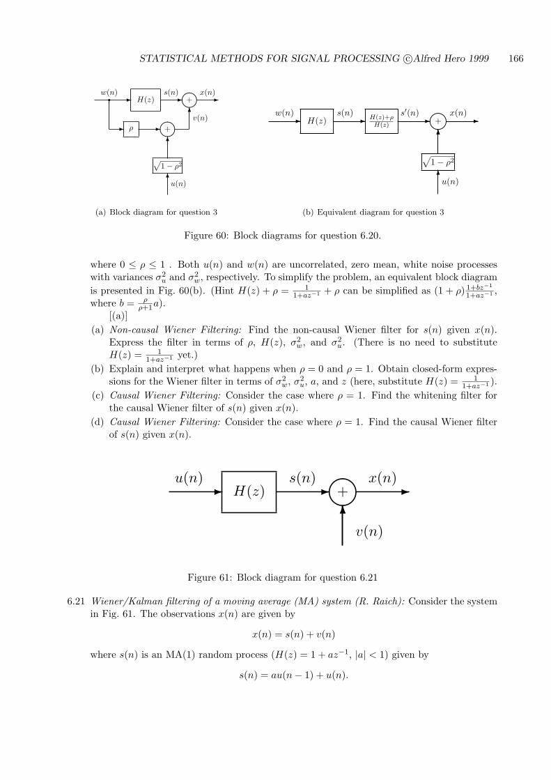
STATISTICAL METHODS FOR SIGNAL PROCESSING c©Alfred Hero 1999 166
w(n)- H(z)
s(n)-
µ´¶³+r
- ρ -µ´¶³
6
+
6v(n)
-x(n)
√1− ρ2
u(n)6
(a) Block diagram for question 3
w(n)- H(z)
s(n)- H(z)+ρ
H(z)-
s′(n)
µ´¶³+
6
√1− ρ2
u(n)6
-x(n)
6
(b) Equivalent diagram for question 3
Figure 60: Block diagrams for question 6.20.
where 0 ≤ ρ ≤ 1 . Both u(n) and w(n) are uncorrelated, zero mean, white noise processeswith variances σ2
u and σ2w, respectively. To simplify the problem, an equivalent block diagram
is presented in Fig. 60(b). (Hint H(z) + ρ = 11+az−1 + ρ can be simplified as (1 + ρ) 1+bz−1
1+az−1 ,where b = ρ
ρ+1a).[(a)]
(a) Non-causal Wiener Filtering: Find the non-causal Wiener filter for s(n) given x(n).Express the filter in terms of ρ, H(z), σ2
w, and σ2u. (There is no need to substitute
H(z) = 11+az−1 yet.)
(b) Explain and interpret what happens when ρ = 0 and ρ = 1. Obtain closed-form expres-sions for the Wiener filter in terms of σ2
w, σ2u, a, and z (here, substitute H(z) = 1
1+az−1 ).(c) Causal Wiener Filtering: Consider the case where ρ = 1. Find the whitening filter for
the causal Wiener filter of s(n) given x(n).(d) Causal Wiener Filtering: Consider the case where ρ = 1. Find the causal Wiener filter
of s(n) given x(n).
u(n)- H(z) -
s(n)
µ´¶³+
6v(n)
-x(n)
6
Figure 61: Block diagram for question 6.21
6.21 Wiener/Kalman filtering of a moving average (MA) system (R. Raich): Consider the systemin Fig. 61. The observations x(n) are given by
x(n) = s(n) + v(n)
where s(n) is an MA(1) random process (H(z) = 1 + az−1, |a| < 1) given by
s(n) = au(n− 1) + u(n).

STATISTICAL METHODS FOR SIGNAL PROCESSING c©Alfred Hero 1999 167
Both v(n) and u(n) are uncorrelated, zero mean, white noise processes with variances σ2v and
σ2u, respectively.
[(a)](a) Non-causal Wiener Filtering: Find the non-causal Wiener filter for s(n) given x(n).(b) Causal Wiener Filtering:
• Find the whitening filter for the causal Wiener filter of s(n) given x(n). (Hint: find asimilar relationship to the one in Exercise 6.3, which is applicable to this question.)
• Find the causal Wiener filter of s(n) given x(n).(c) Kalman Filtering: Derive the Kalman filter for s(n) given x(n). (Hint: choose the state
vector as ξn
= [u(n), u(n− 1)]T ).
(d) Kalman Filtering: Find the steady state Kalman gain in terms of a, σ2v , and σ2
u.
6.22 Let sk be a signal satisfying the AR(1) recursion sk+1 = ask + wk, −∞ < k < ∞, wherea = 0.75 and wk is white noise with variance σ2
w = 1. The signal sk is observed in uncorrelatedwhite noise vk of variance σ2
v = 1:
xk = sk + vk, −∞ ≤ k < ∞.
It is desired to estimate gk = sk − 12sk−1.
(a) Find the non-causal Wiener filter for estimating gk.(b) Find the causal Wiener filter for estimating gk.(c) If Hncw is the non-causal Wiener filter for estimating sk and snc
k is the output of thisfilter, compare the estimator of part (a) to the estimator gnc
k = snck − 1
2 snck−1. Comment
on the difference between these estimators. Which one gives lower MSE?.(d) If Hcw is the causal Wiener filter for estimating sk and sc
k is the output of this filter,compare the estimator of part (b) to the estimator gc
k = sck − 1
2 sck−1. Comment on the
difference between these estimators. Which one gives lower MSE?
6.23 Available for observation is a zero mean w.s.s. signal s(n) in additive white noise v(n) ofvariance σ2
v :x(n) = s(n) + v(n),
where s(n) and v(n) are uncorrelated and s(n) obeys the recursion
s(n) = as(n− 2) + w(n)
and |a| < 1, w(n) is zero mean white noise with variance 1. The objective is to estimate thesignal g(k) = s(k + α) for α ≥ 0 a non-negative integer.
(a) Derive the power spectral density Px(z)of x(n) in terms of a and σ2v .
(b) Plot the pole zero constellation of Px and find the spectral factors P+x (z) and P−x (z).
(c) Derive the cross spectral density Pgx(z).(d) Find the non-causal Wiener filter. To what does your filter reduce when σ2
v = 0 andα = 1?
(e) Find the causal Wiener filter for estimating gk when σ2v = 0. Specialize to the case of
α = 1 and compare to your answer for part (d).(f) Find the causal Wiener filter for σ2
v > 0.
STATISTICAL METHODS FOR SIGNAL PROCESSING c©Alfred Hero 1999 168
6.24 Oftentimes there are outliers or missing observations that prevent direct implementation ofthe Kalman filter. In this problem you will explore one way to handle this scenario. You aregiven an observation model similar to the model (65) in Chapter 6.
xk = sk + vk
sk = cT ξk
ξk+1
= Aξk
+ Bwk
where everything is the same as for (65) except that the observation noise vk has varianceσ2
v(k) that is itself a random variable with two states, a good state (small variance) and abad state (large variance). This can be modeled by introducing a random switching variablebk into the definition of σ2
v(k)
σ2(k) = bkσ20 + (1− bk)σ2
1
where σ20 < σ2
1, and bk are i.i.d. Bernoulli random variables with P (bk = 1) = p andP (bk = 0) = 1− p. We assume that the bk’s are independent of the states ξ
k. This model
introduces missing observations by taking the limit of expressions for the optimal predictorsas σ2
1 →∞. To handle the case of unobserved switching variables we will assume in (b), (c)and (d) that the noises vk, wk and the initial state ξ
0are independent Gaussian distributed.
(a) For the case that the measurements xk and the switching variables bk are both observed,i.e. the outlier indices are known, give the filtering equations for the Kalman filter esti-mator of sk given (xk, bk), (xk−1, bk−1), . . . , (x0, b0). Be sure to specify the state estimatorupdates, the Kalman gain, and the error covariance updates in terms of bk.
(b) To what do your equations in part (a) converge as σ21 → ∞? How about as σ2
1 → σ20?
How do your state update equations compare to those of the standard Kalman filter?(c) Show that the conditional density fξ
k+1|ξ
k(ξ|ξ
k) has the form of a multivariate Gaussian
density and specify the mean and covariance matrix of this conditional density.(d) For the case of unobserved switching variables, find an expression for the instantaneous
state likelihood function fxk|ξk(x|ξ) in terms of the switching probability p. (Hint: you
will need to ”integrate out” the switching variables).
(e) Use Bayes theorem to show that the posterior density of the state, ρk(ξk) def= fξ
k|Xk
(ξk|Xk),
where Xk = xk, xk−1, . . . , x0, obeys the recursion
ρk+1(ξk+1) =
fxk+1|ξk+1(xk+1|ξk+1
)
fxk+1|Xk(xk+1|Xk)
∫fξ
k+1|ξ
k(ξ
k+1|ξ
k)ρk(ξk
)dξk.
where the density fξk+1
|ξk(ξ
k+1|ξ
k) has the form of a multivariate Gaussian density. This
recursion can be used to generate an update equation for the conditional mean stateestimator (see part (f)).
(f) (Extra Credit) Use the recursion (e) to find a time update of the conditional meansk|k = E[sk|Xk] of the form sk|k → sk+1|k+1. You may specialize to the AR(1) model forsk = ξ
kas in homework problem (6.14) and assume low SNR, e.g., a2/σ2
1, σ2w/σ2
1 << 1.
End of chapter
STATISTICAL METHODS FOR SIGNAL PROCESSING c©Alfred Hero 1999 169
7 FUNDAMENTALS OF DETECTION
Next we treat the problem of detection: this is equivalent to estimation when there are only asmall number of possible values for the unknown parameter θ. Some may argue that detection hasa simpler and more elegant theory than estimation, and this might be true depending on the ”eyeof the beholder.” However, as we will see in the next chapter detection and estimation are closelylinked when there exist unknown nuisance parameters that can confound our detection algorithms.
We will cover the following in this chapter
* Optimal detection theory
* Bayesian approach to detection
* Frequentist approach to detection
* Reciever Operating Characteristic (ROC) curves
* Multiple hypothesis testing
Example 31 A motivating radar example
We start with a practical example to motivate the detection theory to come later. Assume thatyou make a continuous time measurement x(t) over a time interval [0, T ] and you wish to decidewhether x(t) is noise alone
x(t) = w(t), 0 ≤ t ≤ T
or whether it is signal plus noise
x(t) = θs(t− τ) + w(t), 0 ≤ t ≤ T.
Here we assume
* s(t) is a known signal that may or may not be present
* w(t) is a zero mean Gaussian white noise with known power spectral density level No/2
*τ is a known time delay, 0 ≤ τ ¿ T
*∫ T0 |s(t− τ)|2dt =
∫ T0 |s(t)|2dt is the signal energy
* θ ∈ 0, 1 unknown nuisance parameter
The detection objective is to decide whether the signal is present or not, and to do this withminimum average number of decision errors.
There is a common notation that has been developed for stating the detection hypotheses: ”nosignal present” (H0) vs ”signal present” (H1)
H0 : x(t) = w(t) H0 : θ = 0⇔
H1 : x(t) = s(t− τ) + w(t) H1 : θ = 1
Without trying to choose a decision function to optimize any particular detection performancecriterion - we will do this later - two methods of detection could be considered, shown in Fig. 62:
Energy-threshold detector:
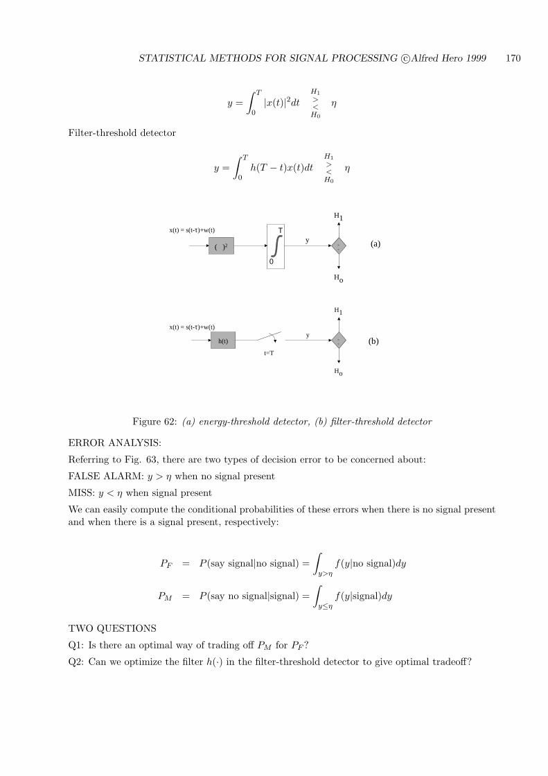
STATISTICAL METHODS FOR SIGNAL PROCESSING c©Alfred Hero 1999 170
y =∫ T
0|x(t)|2dt
H1
><H0
η
Filter-threshold detector
y =∫ T
0h(T − t)x(t)dt
H1
><H0
η
Ho
H1
h(t) ><
y
t=T
x(t) = s(t-τ)+w(t)
Ho
H1
( )2 ><
y (a)
(b)
x(t) = s(t-τ)+w(t) Τ
0
Figure 62: (a) energy-threshold detector, (b) filter-threshold detector
ERROR ANALYSIS:
Referring to Fig. 63, there are two types of decision error to be concerned about:
FALSE ALARM: y > η when no signal present
MISS: y < η when signal present
We can easily compute the conditional probabilities of these errors when there is no signal presentand when there is a signal present, respectively:
PF = P (say signal|no signal) =∫
y>ηf(y|no signal)dy
PM = P (say no signal|signal) =∫
y≤ηf(y|signal)dy
TWO QUESTIONS
Q1: Is there an optimal way of trading off PM for PF ?
Q2: Can we optimize the filter h(·) in the filter-threshold detector to give optimal tradeoff?
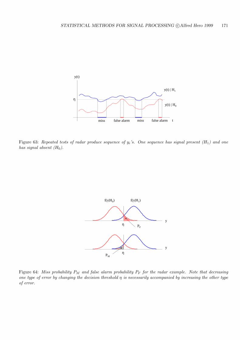
STATISTICAL METHODS FOR SIGNAL PROCESSING c©Alfred Hero 1999 171
y(t)
t
y(t) | H1
y(t) | H0
miss false alarm miss false alarm
η
Figure 63: Repeated tests of radar produce sequence of yi’s. One sequence has signal present (H1) and onehas signal absent (H0).
η PF
f(y|H1)f(y|H0)
ηPM
y
y
Figure 64: Miss probability PM and false alarm probability PF for the radar example. Note that decreasingone type of error by changing the decision threshold η is necessarily accompanied by increasing the other typeof error.
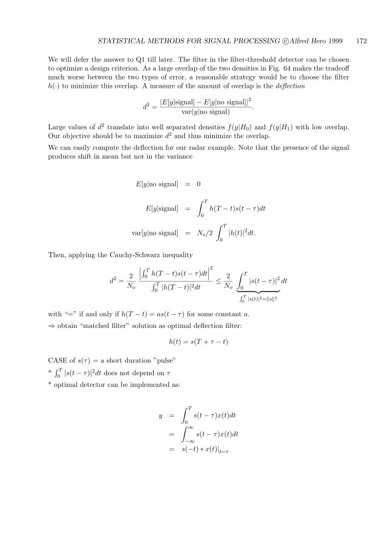
STATISTICAL METHODS FOR SIGNAL PROCESSING c©Alfred Hero 1999 172
We will defer the answer to Q1 till later. The filter in the filter-threshold detector can be chosento optimize a design criterion. As a large overlap of the two densities in Fig. 64 makes the tradeoffmuch worse between the two types of error, a reasonable strategy would be to choose the filterh(·) to minimize this overlap. A measure of the amount of overlap is the deflection
d2 =|E[y|signal]− E[y|no signal]|2
var(y|no signal).
Large values of d2 translate into well separated densities f(y|H0) and f(y|H1) with low overlap.Our objective should be to maximize d2 and thus minimize the overlap.
We can easily compute the deflection for our radar example. Note that the presence of the signalproduces shift in mean but not in the variance
E[y|no signal] = 0
E[y|signal] =∫ T
0h(T − t)s(t− τ)dt
var[y|no signal] = No/2∫ T
0|h(t)|2dt.
Then, applying the Cauchy-Schwarz inequality
d2 =2
No
∣∣∣∫ T0 h(T − t)s(t− τ)dt
∣∣∣2
∫ T0 |h(T − t)|2dt
≤ 2No
∫ T
0|s(t− τ)|2
︸ ︷︷ ︸R T0 |s(t)|2=‖s‖2
dt
with “=” if and only if h(T − t) = as(t− τ) for some constant a.
⇒ obtain “matched filter” solution as optimal deflection filter:
h(t) = s(T + τ − t)
CASE of s(τ) = a short duration ”pulse”
*∫ T0 |s(t− τ)|2dt does not depend on τ
* optimal detector can be implemented as:
y =∫ T
0s(t− τ)x(t)dt
=∫ ∞
−∞s(t− τ)x(t)dt
= s(−t) ∗ x(t)|t=τ
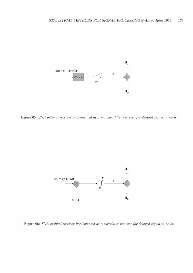
STATISTICAL METHODS FOR SIGNAL PROCESSING c©Alfred Hero 1999 173
Ho
H1
s(T+ τ -t) ><
y
t=T
x(t) = s(t-τ)+w(t)
Figure 65: SNR optimal receiver implemented as a matched filter reciever for delayed signal in noise.
Ho
H1
><
y x(t) = s(t-τ)+w(t)
s(t-τ)
Τ
0
Figure 66: SNR optimal receiver implemented as a correlator reciever for delayed signal in noise.
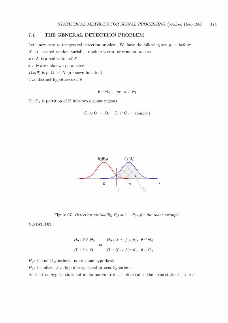
STATISTICAL METHODS FOR SIGNAL PROCESSING c©Alfred Hero 1999 174
7.1 THE GENERAL DETECTION PROBLEM
Let’s now turn to the general detection problem. We have the following setup, as before:
X a measured random variable, random vector, or random process
x ∈ X is a realization of X
θ ∈ Θ are unknown parameters
f(x; θ) is p.d.f. of X (a known function)
Two distinct hypotheses on θ
θ ∈ Θ0, or θ ∈ Θ1
Θ0,Θ1 is partition of Θ into two disjoint regions
Θ0 ∪Θ1 = Θ, Θ0 ∩Θ1 = empty
0 y
f(y|H0) f(y|H1)
µ1
PDη
Figure 67: Detection probability PD = 1− PM for the radar example.
NOTATION:
H0 : θ ∈ Θ0 H0 : X ∼ f(x; θ), θ ∈ Θ0
⇔H1 : θ ∈ Θ1 H1 : X ∼ f(x; θ), θ ∈ Θ1
H0: the null hypothesis, noise alone hypothesis
H1: the alternative hypothesis, signal present hypothesis
As the true hypothesis is not under our control it is often called the ”true state of nature.”

STATISTICAL METHODS FOR SIGNAL PROCESSING c©Alfred Hero 1999 175
Θ
Θ1
Θ0
Figure 68: The detector must decide on the region of Θ that contains the unknown parameter θ.
7.1.1 SIMPLE VS COMPOSITE HYPOTHESES
When θ can take on only two values and Θ0 and Θ1 are singleton sets, the hypotheses are said tobe simple.
Θ = θ0, θ1, Θ0 = θ0, Θ1 = θ1.In this case the p.d.f. f(x; θ) is completely known given either H0 or H1
If the hypotheses are not simple then at least one of Θ1 or Θ0 is not a singleton and is said to becomposite. Simple hypotheses are much easier to deal with and one is lucky to encounter them inpractical problems!
7.1.2 THE DECISION FUNCTION
Detection objective: design a decision rule (test function)
φ(x) =
1, decide H1
0, decide H0.
The test function φ(x) maps X to the decision space 0, 1 for deciding H0 and H1. The functionφ(x) induces a partition of X into decision regions
X0 = x : φ(x) = 0, X1 = x : φ(x) = 1
FALSE ALARM AND MISS ERRORS
False alarm and miss probabilities associated with the test function φ can be expressed simply:
PF (θ) = Eθ[φ] =∫
Xφ(x)f(x; θ)dx, θ ∈ Θ0,
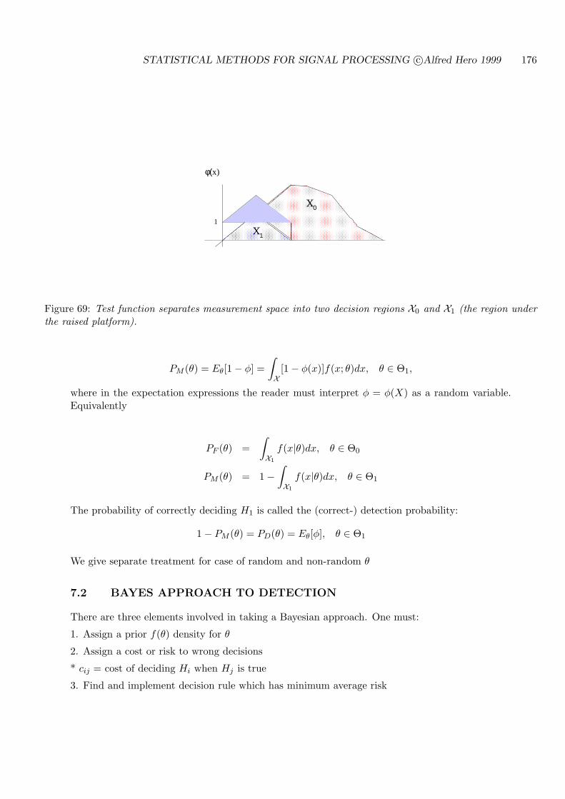
STATISTICAL METHODS FOR SIGNAL PROCESSING c©Alfred Hero 1999 176
φ(x)
1
;0
;1
Figure 69: Test function separates measurement space into two decision regions X0 and X1 (the region underthe raised platform).
PM (θ) = Eθ[1− φ] =∫
X[1− φ(x)]f(x; θ)dx, θ ∈ Θ1,
where in the expectation expressions the reader must interpret φ = φ(X) as a random variable.Equivalently
PF (θ) =∫
X1
f(x|θ)dx, θ ∈ Θ0
PM (θ) = 1−∫
X1
f(x|θ)dx, θ ∈ Θ1
The probability of correctly deciding H1 is called the (correct-) detection probability:
1− PM (θ) = PD(θ) = Eθ[φ], θ ∈ Θ1
We give separate treatment for case of random and non-random θ
7.2 BAYES APPROACH TO DETECTION
There are three elements involved in taking a Bayesian approach. One must:
1. Assign a prior f(θ) density for θ
2. Assign a cost or risk to wrong decisions
* cij = cost of deciding Hi when Hj is true
3. Find and implement decision rule which has minimum average risk
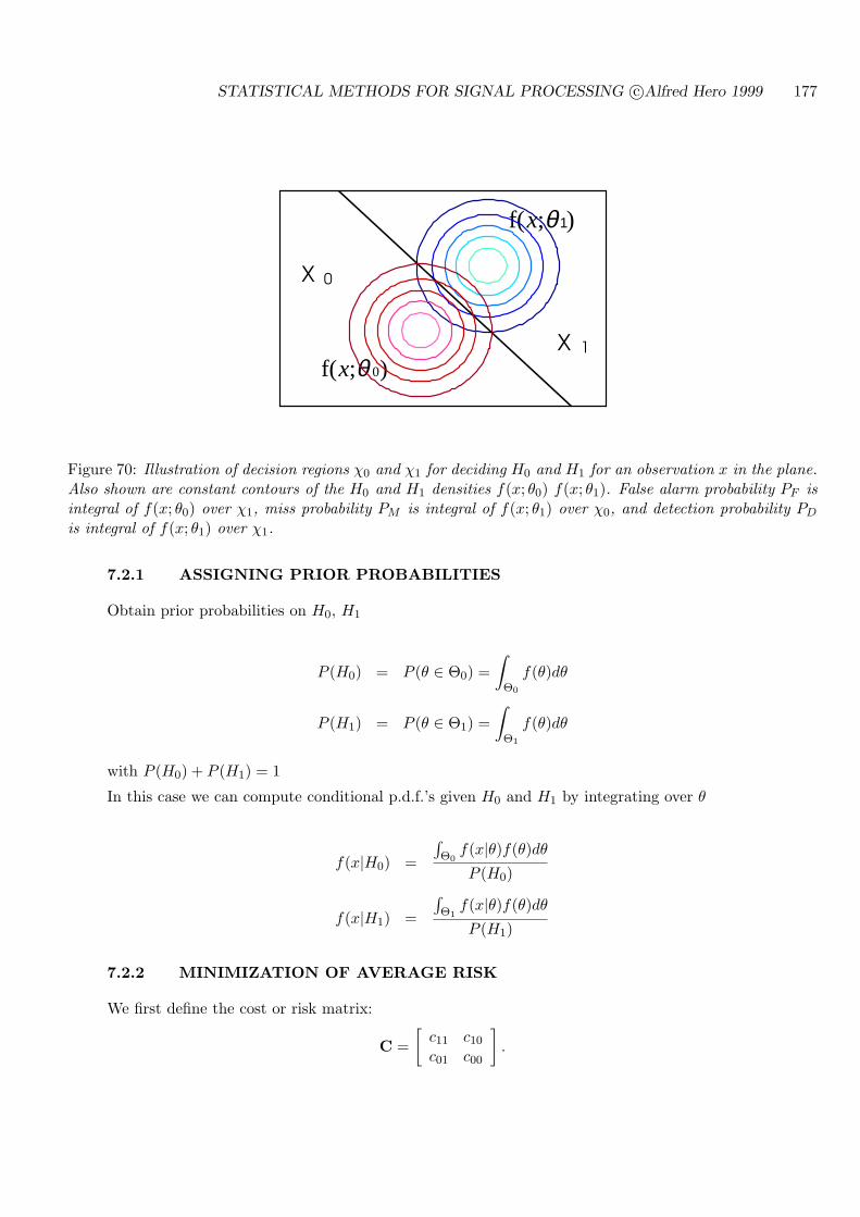
STATISTICAL METHODS FOR SIGNAL PROCESSING c©Alfred Hero 1999 177
);f( 1θx
);f( 0θx
X 0
X 1
Figure 70: Illustration of decision regions χ0 and χ1 for deciding H0 and H1 for an observation x in the plane.Also shown are constant contours of the H0 and H1 densities f(x; θ0) f(x; θ1). False alarm probability PF isintegral of f(x; θ0) over χ1, miss probability PM is integral of f(x; θ1) over χ0, and detection probability PD
is integral of f(x; θ1) over χ1.
7.2.1 ASSIGNING PRIOR PROBABILITIES
Obtain prior probabilities on H0, H1
P (H0) = P (θ ∈ Θ0) =∫
Θ0
f(θ)dθ
P (H1) = P (θ ∈ Θ1) =∫
Θ1
f(θ)dθ
with P (H0) + P (H1) = 1
In this case we can compute conditional p.d.f.’s given H0 and H1 by integrating over θ
f(x|H0) =
∫Θ0
f(x|θ)f(θ)dθ
P (H0)
f(x|H1) =
∫Θ1
f(x|θ)f(θ)dθ
P (H1)
7.2.2 MINIMIZATION OF AVERAGE RISK
We first define the cost or risk matrix:
C =[
c11 c10
c01 c00
].
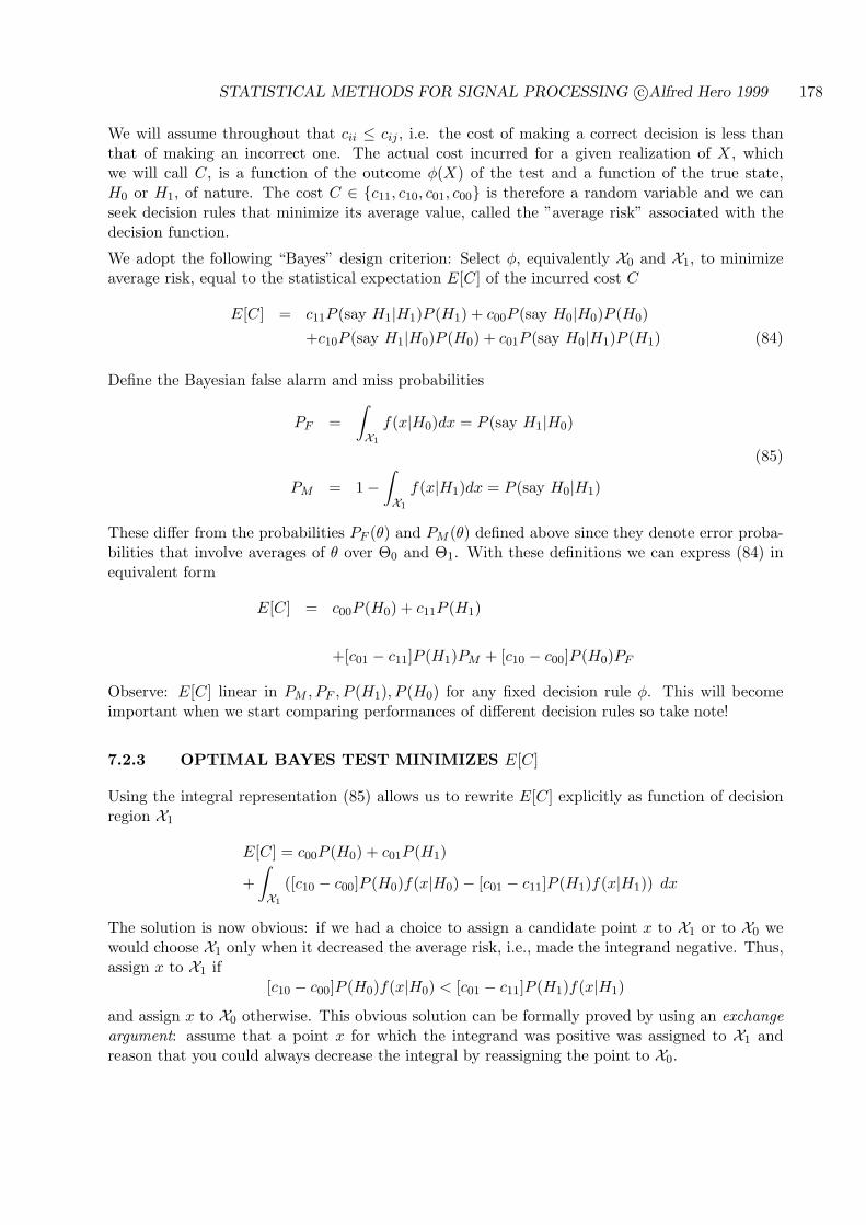
STATISTICAL METHODS FOR SIGNAL PROCESSING c©Alfred Hero 1999 178
We will assume throughout that cii ≤ cij , i.e. the cost of making a correct decision is less thanthat of making an incorrect one. The actual cost incurred for a given realization of X, whichwe will call C, is a function of the outcome φ(X) of the test and a function of the true state,H0 or H1, of nature. The cost C ∈ c11, c10, c01, c00 is therefore a random variable and we canseek decision rules that minimize its average value, called the ”average risk” associated with thedecision function.
We adopt the following “Bayes” design criterion: Select φ, equivalently X0 and X1, to minimizeaverage risk, equal to the statistical expectation E[C] of the incurred cost C
E[C] = c11P (say H1|H1)P (H1) + c00P (say H0|H0)P (H0)+c10P (say H1|H0)P (H0) + c01P (say H0|H1)P (H1) (84)
Define the Bayesian false alarm and miss probabilities
PF =∫
X1
f(x|H0)dx = P (say H1|H0)
(85)
PM = 1−∫
X1
f(x|H1)dx = P (say H0|H1)
These differ from the probabilities PF (θ) and PM (θ) defined above since they denote error proba-bilities that involve averages of θ over Θ0 and Θ1. With these definitions we can express (84) inequivalent form
E[C] = c00P (H0) + c11P (H1)
+[c01 − c11]P (H1)PM + [c10 − c00]P (H0)PF
Observe: E[C] linear in PM , PF , P (H1), P (H0) for any fixed decision rule φ. This will becomeimportant when we start comparing performances of different decision rules so take note!
7.2.3 OPTIMAL BAYES TEST MINIMIZES E[C]
Using the integral representation (85) allows us to rewrite E[C] explicitly as function of decisionregion X1
E[C] = c00P (H0) + c01P (H1)
+∫
X1
([c10 − c00]P (H0)f(x|H0)− [c01 − c11]P (H1)f(x|H1)) dx
The solution is now obvious: if we had a choice to assign a candidate point x to X1 or to X0 wewould choose X1 only when it decreased the average risk, i.e., made the integrand negative. Thus,assign x to X1 if
[c10 − c00]P (H0)f(x|H0) < [c01 − c11]P (H1)f(x|H1)
and assign x to X0 otherwise. This obvious solution can be formally proved by using an exchangeargument: assume that a point x for which the integrand was positive was assigned to X1 andreason that you could always decrease the integral by reassigning the point to X0.
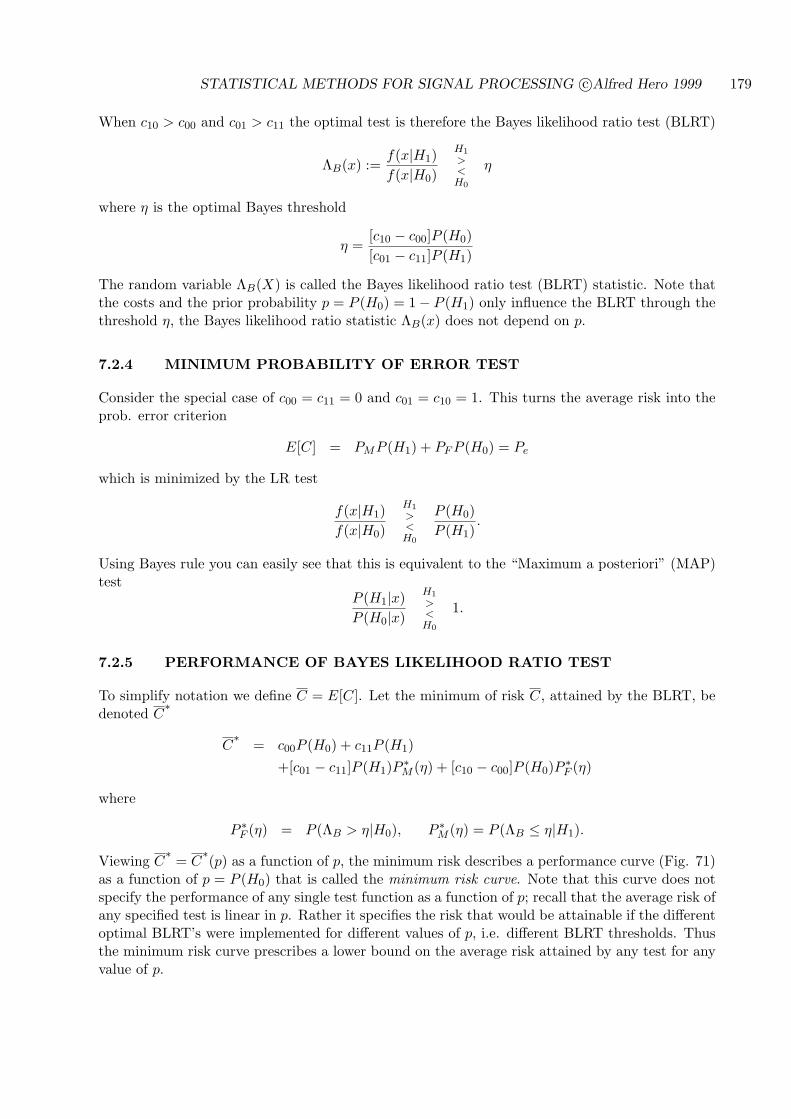
STATISTICAL METHODS FOR SIGNAL PROCESSING c©Alfred Hero 1999 179
When c10 > c00 and c01 > c11 the optimal test is therefore the Bayes likelihood ratio test (BLRT)
ΛB(x) :=f(x|H1)f(x|H0)
H1
><H0
η
where η is the optimal Bayes threshold
η =[c10 − c00]P (H0)[c01 − c11]P (H1)
The random variable ΛB(X) is called the Bayes likelihood ratio test (BLRT) statistic. Note thatthe costs and the prior probability p = P (H0) = 1− P (H1) only influence the BLRT through thethreshold η, the Bayes likelihood ratio statistic ΛB(x) does not depend on p.
7.2.4 MINIMUM PROBABILITY OF ERROR TEST
Consider the special case of c00 = c11 = 0 and c01 = c10 = 1. This turns the average risk into theprob. error criterion
E[C] = PMP (H1) + PF P (H0) = Pe
which is minimized by the LR test
f(x|H1)f(x|H0)
H1
><H0
P (H0)P (H1)
.
Using Bayes rule you can easily see that this is equivalent to the “Maximum a posteriori” (MAP)test
P (H1|x)P (H0|x)
H1
><H0
1.
7.2.5 PERFORMANCE OF BAYES LIKELIHOOD RATIO TEST
To simplify notation we define C = E[C]. Let the minimum of risk C, attained by the BLRT, bedenoted C
∗
C∗ = c00P (H0) + c11P (H1)
+[c01 − c11]P (H1)P ∗M (η) + [c10 − c00]P (H0)P ∗
F (η)
where
P ∗F (η) = P (ΛB > η|H0), P ∗
M (η) = P (ΛB ≤ η|H1).
Viewing C∗ = C
∗(p) as a function of p, the minimum risk describes a performance curve (Fig. 71)as a function of p = P (H0) that is called the minimum risk curve. Note that this curve does notspecify the performance of any single test function as a function of p; recall that the average risk ofany specified test is linear in p. Rather it specifies the risk that would be attainable if the differentoptimal BLRT’s were implemented for different values of p, i.e. different BLRT thresholds. Thusthe minimum risk curve prescribes a lower bound on the average risk attained by any test for anyvalue of p.
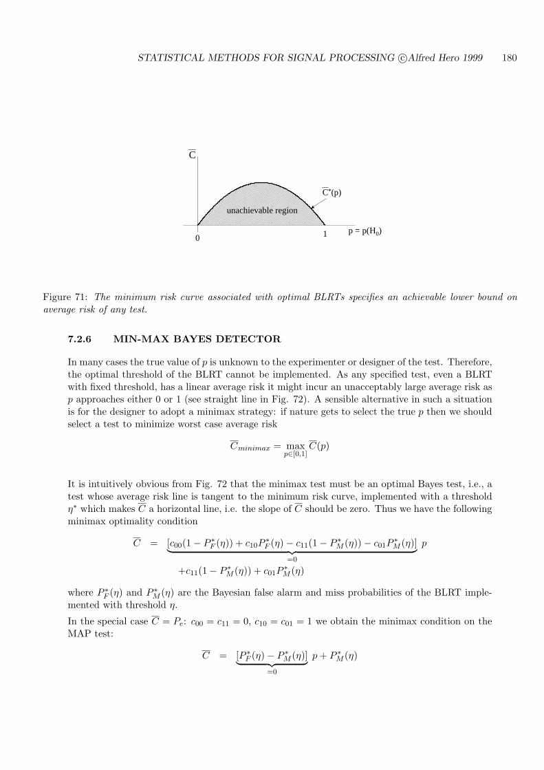
STATISTICAL METHODS FOR SIGNAL PROCESSING c©Alfred Hero 1999 180
unachievable region
0 1
C
p)(C*
p = p(H0)
Figure 71: The minimum risk curve associated with optimal BLRTs specifies an achievable lower bound onaverage risk of any test.
7.2.6 MIN-MAX BAYES DETECTOR
In many cases the true value of p is unknown to the experimenter or designer of the test. Therefore,the optimal threshold of the BLRT cannot be implemented. As any specified test, even a BLRTwith fixed threshold, has a linear average risk it might incur an unacceptably large average risk asp approaches either 0 or 1 (see straight line in Fig. 72). A sensible alternative in such a situationis for the designer to adopt a minimax strategy: if nature gets to select the true p then we shouldselect a test to minimize worst case average risk
Cminimax = maxp∈[0,1]
C(p)
It is intuitively obvious from Fig. 72 that the minimax test must be an optimal Bayes test, i.e., atest whose average risk line is tangent to the minimum risk curve, implemented with a thresholdη∗ which makes C a horizontal line, i.e. the slope of C should be zero. Thus we have the followingminimax optimality condition
C = [c00(1− P ∗F (η)) + c10P
∗F (η)− c11(1− P ∗
M (η))− c01P∗M (η)]︸ ︷︷ ︸
=0
p
+c11(1− P ∗M (η)) + c01P
∗M (η)
where P ∗F (η) and P ∗
M (η) are the Bayesian false alarm and miss probabilities of the BLRT imple-mented with threshold η.
In the special case C = Pe: c00 = c11 = 0, c10 = c01 = 1 we obtain the minimax condition on theMAP test:
C = [P ∗F (η)− P ∗
M (η)]︸ ︷︷ ︸=0
p + P ∗M (η)
STATISTICAL METHODS FOR SIGNAL PROCESSING c©Alfred Hero 1999 181
(p)Cmax φp
(p)Cφ
minmax )(C (p)C*
p=φ
)p(*C
p*0 1 p = p(H0)
Figure 72: Power curve of any fixed test φ is a straight line. The minimax optimal test φ∗ has a horizontalpower curve which is tangent to the minimum risk, denoted C
∗(p), at its maximum.
This implies that η should be selected so as to ensure the “equalization” condition is satsified
P ∗F (η) = P (ΛB > η|H0) = P (ΛB ≤ η|H1) = P ∗
M (η).
Denoting this minimax value of η as η∗, and noting that the designer can choose a threshold bychoosing (guessing) a value of p, the minimax threshold is related to a minimax choice p∗ throughthe relation η∗ = p∗/(1− p∗).
7.2.7 EXAMPLES
Example 32 Radar example revisited
Objective: Given the matched filter output y find the Bayes optimal detector.
1. Assume that P (H0) = P (H1) = 12
2. Recall that y is
y =∫ T
0s(t)x(t)dt
which is a realization of a Gaussian random variable Y having means and variances
E[Y |H0] = 0, var[Y |H0] = No/2∫ T0 |s(t)|2dt = σ2
0
E[Y |H1] =∫ T0 |s(t)|2dt = µ1, var[Y |H1] = No/2
∫ T0 |s(t)|2dt = σ2
0
Bayes LR test is
STATISTICAL METHODS FOR SIGNAL PROCESSING c©Alfred Hero 1999 182
ΛB(y) =
1√2πσ2
0
e− 1
2σ20(y−µ1)2
1√2πσ2
0
e− 1
2σ20
y2
= eyµ1/σ20− 1
2µ21/σ2
0
H1
><H0
η = 1
LR test statistic ΛB(Y ) is a monotone function of Y since µ1 > 0.
Equivalent test is filter-threshold detector
YH1
><H0
γ = 12µ1
Performance of Bayes LRT for radar example
PF = P (Y > γ|H0)= P (Y/σ0︸ ︷︷ ︸
N (0,1)
> γ/σ0|H0)
=∫ ∞
γ/σ0
1√2π
e−u2/2du
= 1−N (γ/σ0) := Q(γ/σ0)
and
PM = P (Y < γ|H1)= P ((Y − µ1)/σ0︸ ︷︷ ︸
N (0,1)
> (γ − µ1)/σ0|H1)
= N ((γ − µ1)/σ0)
Note: since the standard Gaussian p.d.f. is symmetric
N (−u) = 1−N (u) and thus, since γ = µ1/2
PM = PF = 1−N (µ1/(2σ0)).
We thus conclude that the Bayes threshold γ is actually minimax! Therefore the probability oferror reduces to
Pe = PM12 + PF
12
= PF

STATISTICAL METHODS FOR SIGNAL PROCESSING c©Alfred Hero 1999 183
-3 -2 -1 0 1 2 30
0.2
0.4
0.6
0.8
1
x
-u u
N(u)
N(-u)=1-N(u)
cdf
Figure 73: CDF N (u) of symmetric Gaussian density
0 y
121 =
f(y|H0) f(y|H1)
µ1
Figure 74: Equally likely hypotheses have minmax threshold γ = 12µ1 for problem of detection of shift in mean
of a Gaussian r.v.
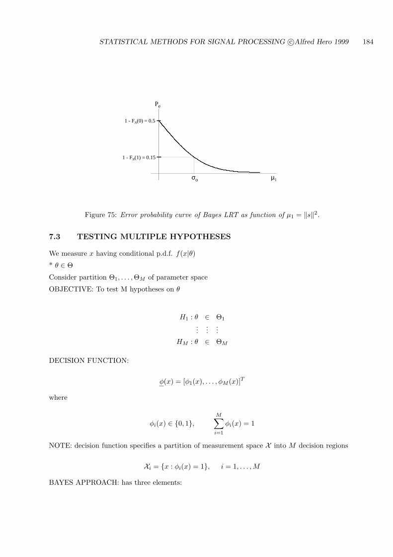
STATISTICAL METHODS FOR SIGNAL PROCESSING c©Alfred Hero 1999 184
1 - FN(0) = 0.5
1 - FN(1) = 0.15
σo
Pe
µ1
Figure 75: Error probability curve of Bayes LRT as function of µ1 = ‖s‖2.
7.3 TESTING MULTIPLE HYPOTHESES
We measure x having conditional p.d.f. f(x|θ)* θ ∈ Θ
Consider partition Θ1, . . . , ΘM of parameter space
OBJECTIVE: To test M hypotheses on θ
H1 : θ ∈ Θ1
......
...HM : θ ∈ ΘM
DECISION FUNCTION:
φ(x) = [φ1(x), . . . , φM (x)]T
where
φi(x) ∈ 0, 1,M∑
i=1
φi(x) = 1
NOTE: decision function specifies a partition of measurement space X into M decision regions
Xi = x : φi(x) = 1, i = 1, . . . ,M
BAYES APPROACH: has three elements:
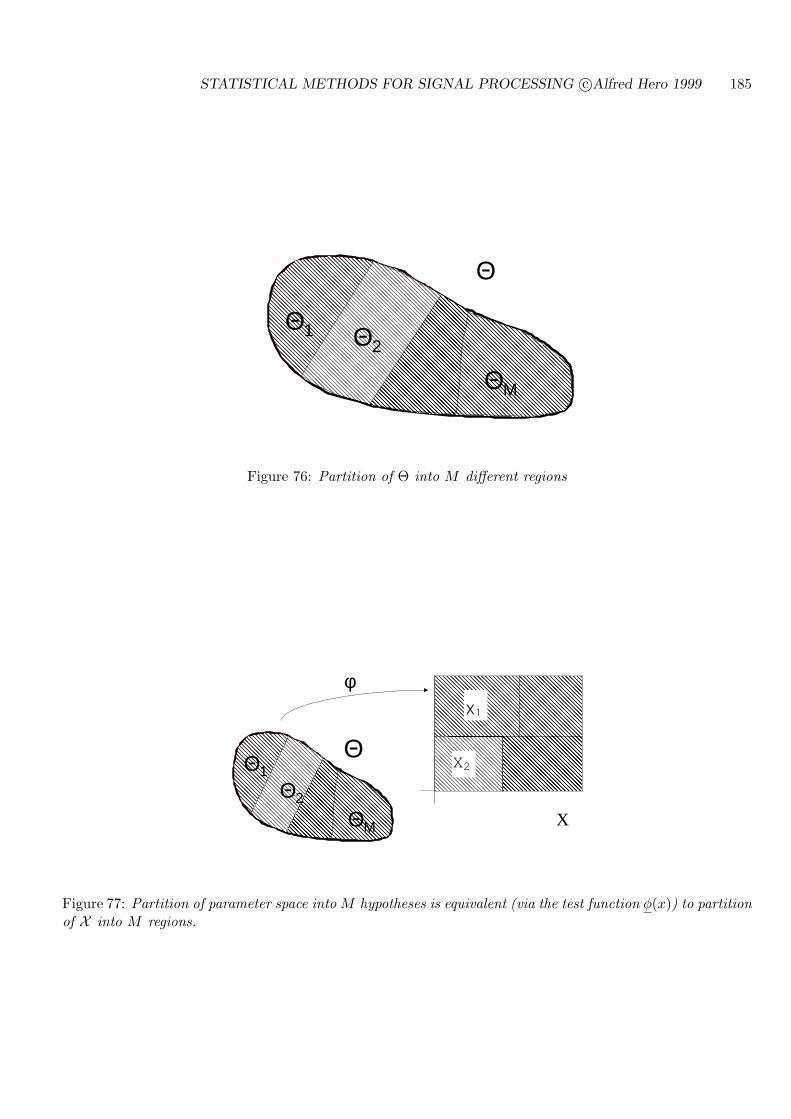
STATISTICAL METHODS FOR SIGNAL PROCESSING c©Alfred Hero 1999 185
Θ
ΘΜ
Θ1 Θ2
Figure 76: Partition of Θ into M different regions
Θ
ΘΜ
Θ1Θ2 rtition
of X
X1
X2
φ
Figure 77: Partition of parameter space into M hypotheses is equivalent (via the test function φ(x)) to partitionof X into M regions.
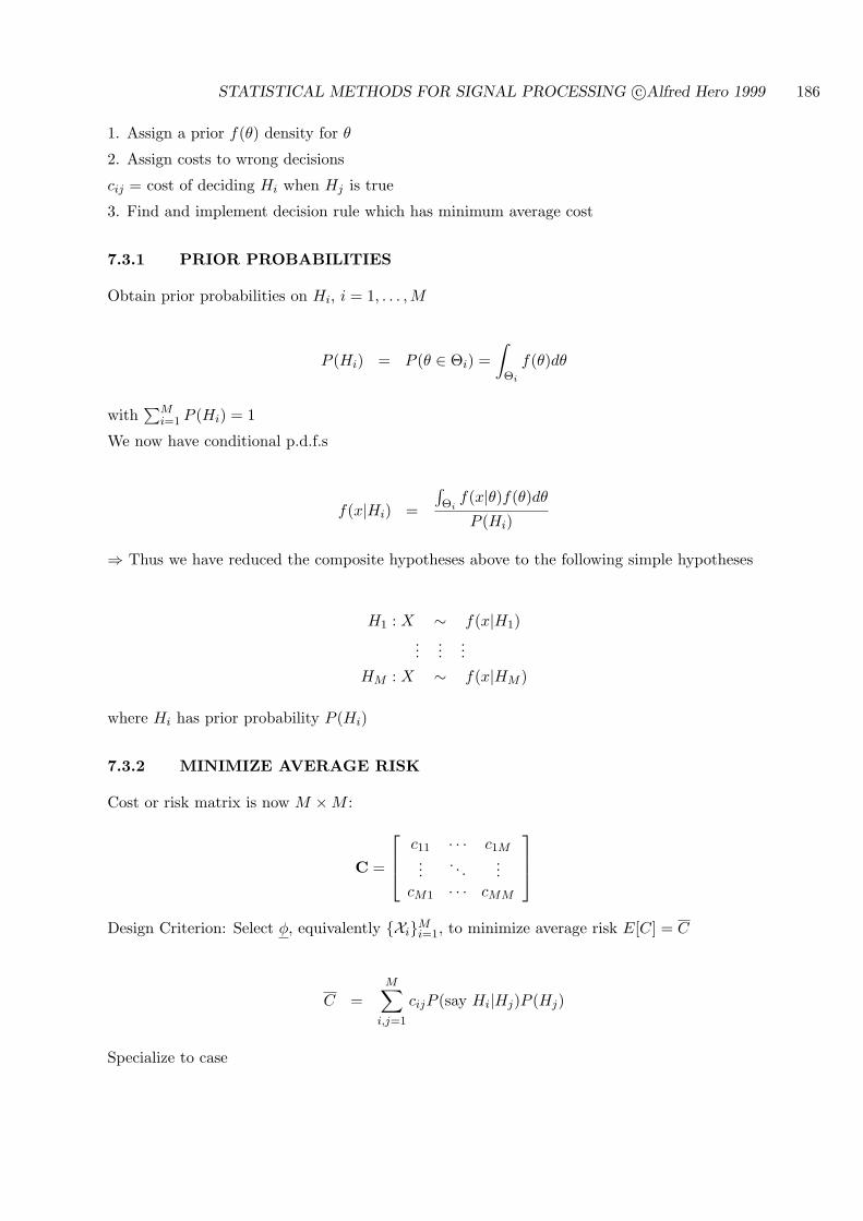
STATISTICAL METHODS FOR SIGNAL PROCESSING c©Alfred Hero 1999 186
1. Assign a prior f(θ) density for θ
2. Assign costs to wrong decisions
cij = cost of deciding Hi when Hj is true
3. Find and implement decision rule which has minimum average cost
7.3.1 PRIOR PROBABILITIES
Obtain prior probabilities on Hi, i = 1, . . . , M
P (Hi) = P (θ ∈ Θi) =∫
Θi
f(θ)dθ
with∑M
i=1 P (Hi) = 1
We now have conditional p.d.f.s
f(x|Hi) =
∫Θi
f(x|θ)f(θ)dθ
P (Hi)
⇒ Thus we have reduced the composite hypotheses above to the following simple hypotheses
H1 : X ∼ f(x|H1)...
......
HM : X ∼ f(x|HM )
where Hi has prior probability P (Hi)
7.3.2 MINIMIZE AVERAGE RISK
Cost or risk matrix is now M ×M :
C =
c11 · · · c1M...
. . ....
cM1 · · · cMM
Design Criterion: Select φ, equivalently XiMi=1, to minimize average risk E[C] = C
C =M∑
i,j=1
cijP (say Hi|Hj)P (Hj)
Specialize to case
STATISTICAL METHODS FOR SIGNAL PROCESSING c©Alfred Hero 1999 187
* cii = 0
* cij = 1, i 6= j
Then we have C = Pe
C =∑
i,j:i6=j
P (say Hi|Hj)P (Hj)
= 1−∑
i,j:i=jP (say Hi|Hj)P (Hj)
= 1−∑
i,j:i=jP (X ∈ Xi|Hi)P (Hi)
= 1−M∑
i=1
∫
Xi
f(x|Hi)dx P (Hi)
Observe: to make C as small as possible
x ∈ Xi ⇔ f(x|Hi)P (Hi) ≥ f(x|Hj)P (Hj), j 6= i
Or in terms of decision function:
φi(x) =
1, f(x|Hi)P (Hi) ≥ f(x|Hj)P (Hj)0, o.w.
Shorthand notation
Hi = Hi(x) = argmaxHjf(x|Hj)P (Hj)
This is equivalent to the “MAP” rule
Hi = argmaxHjP (Hj |x)
REMARKS:
* MAP decision rule minimizes average Pe
* Minimum average Pe is equal to
P ∗e = 1−
M∑
i=1
E[φi(x)|Hi]P (Hi)
* MAP decision rule on x depends only through LR = sufficient statistic
* For equally likely Hi, P (Hi) = 1/M and MAP test is of form
Hi = argmaxHjf(x|Hj)
which should be read: “estimate Hi = H1 if f(x|H1) > f(x|H0).” This can be interpreted as the“Maximum likelihood” estimate of true hypothesis Hj

STATISTICAL METHODS FOR SIGNAL PROCESSING c©Alfred Hero 1999 188
Example 33 Classifier of Gaussian Means
* X = [X1, . . . , Xn]T are i.i.d. N (µ, σ2)
* σ2 is known
OBJECTIVE: classify µ among three possible values
H1 : µ = µ1
H2 : µ = µ2
H3 : µ = µ3
Assume equally likely hypotheses
We know that MAP classifier depends on the X only through sufficient statistic for µ:
X = n−1n∑
i=1
Xi
which is Gaussian with mean µ and variance σ2/n.
Therefore, the MAP test is of form:
Decide Hk iff
f(X|Hk) ≥ f(X|Hj)
where
f(x|Hk) =1√
2πσ2/nexp
(− 1
2σ2/n(X − µk)2
)
or eliminating common factors and taking logarithm
Xµk − 12µ
2k ≥ Xµj − 1
2µ2j
⇒ Linear decision regions!
Concrete example: µ1 = −1, µ2 = +1 , µ3 = 2
Plot 3 lines as a function of X to find the decision regions:
X1 = X : X ≤ 0X2 = X : 0 < X ≤ 3/2X3 = X : X ≥ 3/2
These are regions separated by hyperplanes in X = IRn.
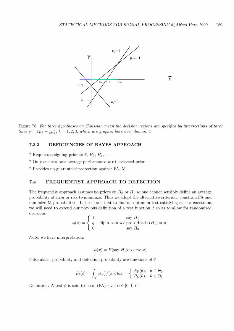
STATISTICAL METHODS FOR SIGNAL PROCESSING c©Alfred Hero 1999 189
1
-1/2
-2
11/2 3/2
y
x
Figure 78: For three hypotheses on Gaussian mean the decision regions are specified by intersections of threelines y = xµk − 1
2µ2k, k = 1, 2, 3, which are graphed here over domain x.
7.3.3 DEFICIENCIES OF BAYES APPROACH
* Requires assigning prior to θ, H0, H1, . . .
* Only ensures best average performance w.r.t. selected prior
* Provides no guaranteed protection against FA, M
7.4 FREQUENTIST APPROACH TO DETECTION
The frequentist approach assumes no priors on H0 or H1 so one cannot sensibly define an averageprobability of error or risk to minimize. Thus we adopt the alternative criterion: constrain FA andminimize M probabilities. It turns out that to find an optimum test satisfying such a constraintwe will need to extend our previous definition of a test function φ so as to allow for randomizeddecisions
φ(x) =
1, say H1
q, flip a coin w/ prob Heads (H1) = q0, say H0
Note, we have interpretation:
φ(x) = P (say H1|observe x)
False alarm probability and detection probability are functions of θ
Eθ[φ] =∫
Xφ(x)f(x; θ)dx =
PF (θ), θ ∈ Θ0
PD(θ), θ ∈ Θ1
Definition: A test φ is said to be of (FA) level α ∈ [0, 1] if
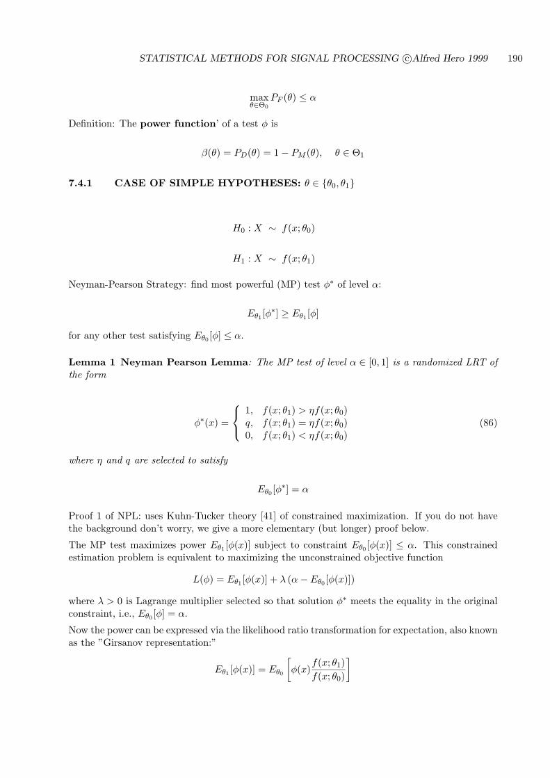
STATISTICAL METHODS FOR SIGNAL PROCESSING c©Alfred Hero 1999 190
maxθ∈Θ0
PF (θ) ≤ α
Definition: The power function’ of a test φ is
β(θ) = PD(θ) = 1− PM (θ), θ ∈ Θ1
7.4.1 CASE OF SIMPLE HYPOTHESES: θ ∈ θ0, θ1
H0 : X ∼ f(x; θ0)
H1 : X ∼ f(x; θ1)
Neyman-Pearson Strategy: find most powerful (MP) test φ∗ of level α:
Eθ1 [φ∗] ≥ Eθ1 [φ]
for any other test satisfying Eθ0 [φ] ≤ α.
Lemma 1 Neyman Pearson Lemma: The MP test of level α ∈ [0, 1] is a randomized LRT ofthe form
φ∗(x) =
1, f(x; θ1) > ηf(x; θ0)q, f(x; θ1) = ηf(x; θ0)0, f(x; θ1) < ηf(x; θ0)
(86)
where η and q are selected to satisfy
Eθ0 [φ∗] = α
Proof 1 of NPL: uses Kuhn-Tucker theory [41] of constrained maximization. If you do not havethe background don’t worry, we give a more elementary (but longer) proof below.
The MP test maximizes power Eθ1 [φ(x)] subject to constraint Eθ0 [φ(x)] ≤ α. This constrainedestimation problem is equivalent to maximizing the unconstrained objective function
L(φ) = Eθ1 [φ(x)] + λ (α− Eθ0 [φ(x)])
where λ > 0 is Lagrange multiplier selected so that solution φ∗ meets the equality in the originalconstraint, i.e., Eθ0 [φ] = α.
Now the power can be expressed via the likelihood ratio transformation for expectation, also knownas the ”Girsanov representation:”
Eθ1 [φ(x)] = Eθ0
[φ(x)
f(x; θ1)f(x; θ0)
]
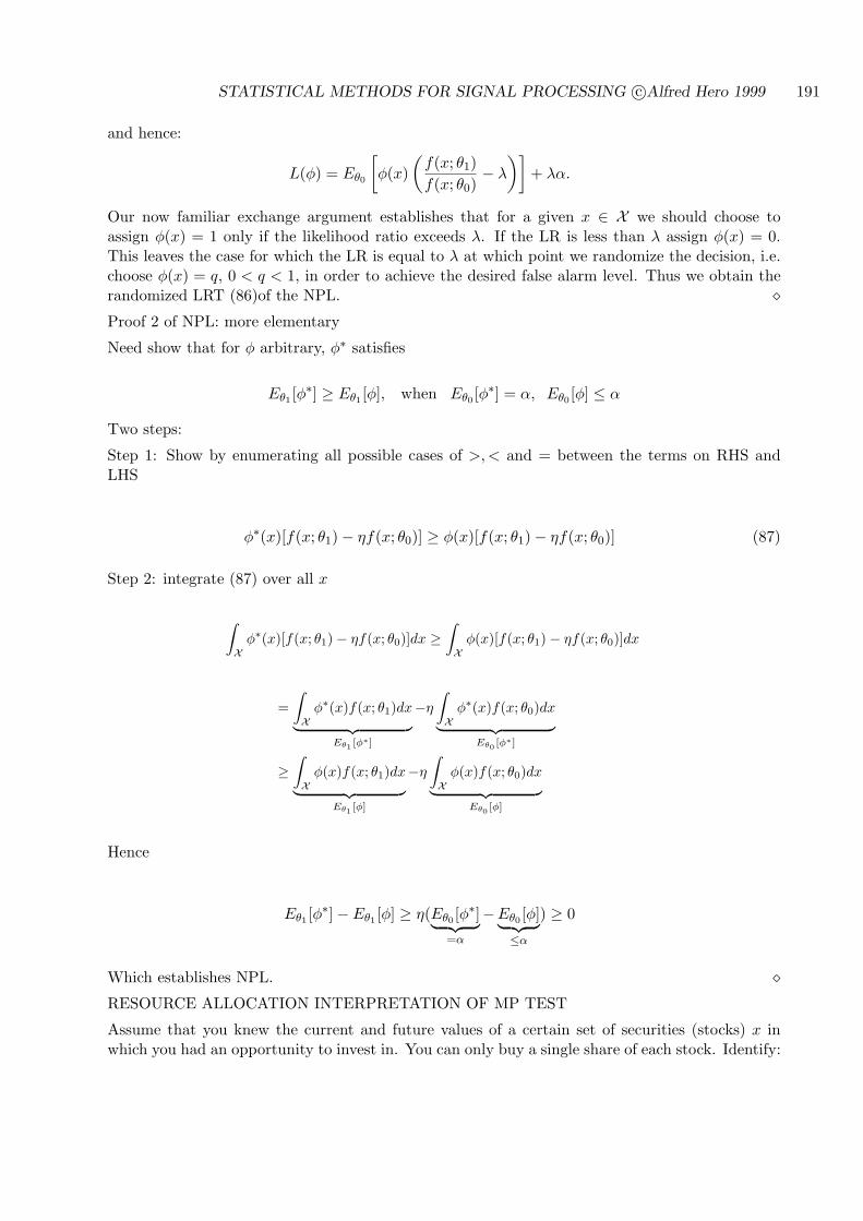
STATISTICAL METHODS FOR SIGNAL PROCESSING c©Alfred Hero 1999 191
and hence:
L(φ) = Eθ0
[φ(x)
(f(x; θ1)f(x; θ0)
− λ
)]+ λα.
Our now familiar exchange argument establishes that for a given x ∈ X we should choose toassign φ(x) = 1 only if the likelihood ratio exceeds λ. If the LR is less than λ assign φ(x) = 0.This leaves the case for which the LR is equal to λ at which point we randomize the decision, i.e.choose φ(x) = q, 0 < q < 1, in order to achieve the desired false alarm level. Thus we obtain therandomized LRT (86)of the NPL. ¦Proof 2 of NPL: more elementary
Need show that for φ arbitrary, φ∗ satisfies
Eθ1 [φ∗] ≥ Eθ1 [φ], when Eθ0 [φ
∗] = α, Eθ0 [φ] ≤ α
Two steps:
Step 1: Show by enumerating all possible cases of >,< and = between the terms on RHS andLHS
φ∗(x)[f(x; θ1)− ηf(x; θ0)] ≥ φ(x)[f(x; θ1)− ηf(x; θ0)] (87)
Step 2: integrate (87) over all x
∫
Xφ∗(x)[f(x; θ1)− ηf(x; θ0)]dx ≥
∫
Xφ(x)[f(x; θ1)− ηf(x; θ0)]dx
=∫
Xφ∗(x)f(x; θ1)dx
︸ ︷︷ ︸Eθ1 [φ∗]
−η
∫
Xφ∗(x)f(x; θ0)dx
︸ ︷︷ ︸Eθ0 [φ∗]
≥∫
Xφ(x)f(x; θ1)dx
︸ ︷︷ ︸Eθ1 [φ]
−η
∫
Xφ(x)f(x; θ0)dx
︸ ︷︷ ︸Eθ0 [φ]
Hence
Eθ1 [φ∗]−Eθ1 [φ] ≥ η(Eθ0 [φ
∗]︸ ︷︷ ︸=α
−Eθ0 [φ]︸ ︷︷ ︸≤α
) ≥ 0
Which establishes NPL. ¦RESOURCE ALLOCATION INTERPRETATION OF MP TEST
Assume that you knew the current and future values of a certain set of securities (stocks) x inwhich you had an opportunity to invest in. You can only buy a single share of each stock. Identify:
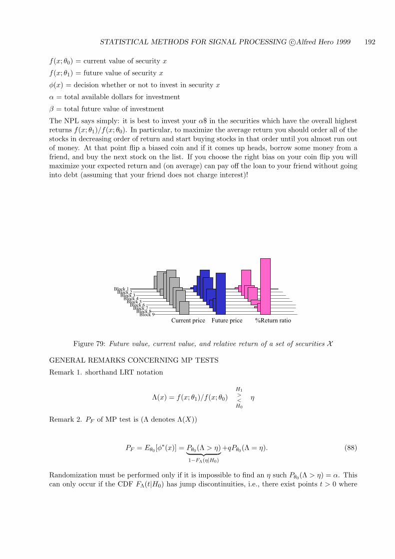
STATISTICAL METHODS FOR SIGNAL PROCESSING c©Alfred Hero 1999 192
f(x; θ0) = current value of security x
f(x; θ1) = future value of security x
φ(x) = decision whether or not to invest in security x
α = total available dollars for investment
β = total future value of investment
The NPL says simply: it is best to invest your α$ in the securities which have the overall highestreturns f(x; θ1)/f(x; θ0). In particular, to maximize the average return you should order all of thestocks in decreasing order of return and start buying stocks in that order until you almost run outof money. At that point flip a biased coin and if it comes up heads, borrow some money from afriend, and buy the next stock on the list. If you choose the right bias on your coin flip you willmaximize your expected return and (on average) can pay off the loan to your friend without goinginto debt (assuming that your friend does not charge interest)!
Current price Future price %Return ratio
Block 1Block 2
Block 3Block 4
Block 5Block 6
Block 7Block 8
Block 9
Figure 79: Future value, current value, and relative return of a set of securities X
GENERAL REMARKS CONCERNING MP TESTS
Remark 1. shorthand LRT notation
Λ(x) = f(x; θ1)/f(x; θ0)H1
><H0
η
Remark 2. PF of MP test is (Λ denotes Λ(X))
PF = Eθ0 [φ∗(x)] = Pθ0(Λ > η)︸ ︷︷ ︸
1−FΛ(η|H0)
+qPθ0(Λ = η). (88)
Randomization must be performed only if it is impossible to find an η such Pθ0(Λ > η) = α. Thiscan only occur if the CDF FΛ(t|H0) has jump discontinuities, i.e., there exist points t > 0 where
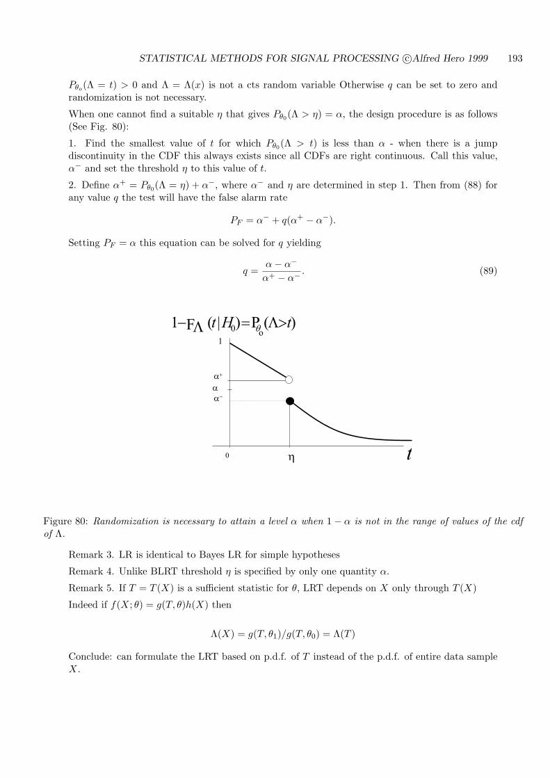
STATISTICAL METHODS FOR SIGNAL PROCESSING c©Alfred Hero 1999 193
Pθo(Λ = t) > 0 and Λ = Λ(x) is not a cts random variable Otherwise q can be set to zero andrandomization is not necessary.
When one cannot find a suitable η that gives Pθ0(Λ > η) = α, the design procedure is as follows(See Fig. 80):
1. Find the smallest value of t for which Pθ0(Λ > t) is less than α - when there is a jumpdiscontinuity in the CDF this always exists since all CDFs are right continuous. Call this value,α− and set the threshold η to this value of t.
2. Define α+ = Pθ0(Λ = η) + α−, where α− and η are determined in step 1. Then from (88) forany value q the test will have the false alarm rate
PF = α− + q(α+ − α−).
Setting PF = α this equation can be solved for q yielding
q =α− α−
α+ − α−. (89)
0
)( P)|(F1o
0 tHt
t
Figure 80: Randomization is necessary to attain a level α when 1− α is not in the range of values of the cdfof Λ.
Remark 3. LR is identical to Bayes LR for simple hypotheses
Remark 4. Unlike BLRT threshold η is specified by only one quantity α.
Remark 5. If T = T (X) is a sufficient statistic for θ, LRT depends on X only through T (X)
Indeed if f(X; θ) = g(T, θ)h(X) then
Λ(X) = g(T, θ1)/g(T, θ0) = Λ(T )
Conclude: can formulate the LRT based on p.d.f. of T instead of the p.d.f. of entire data sampleX.
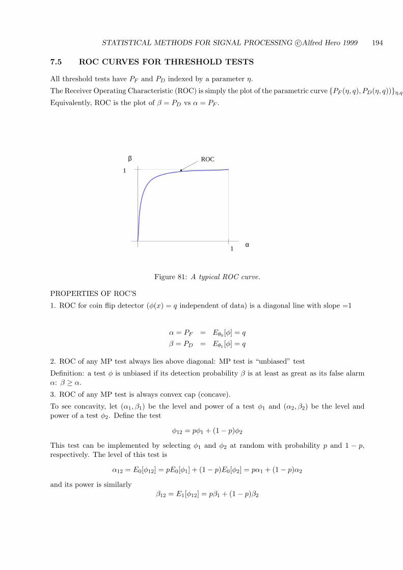
STATISTICAL METHODS FOR SIGNAL PROCESSING c©Alfred Hero 1999 194
7.5 ROC CURVES FOR THRESHOLD TESTS
All threshold tests have PF and PD indexed by a parameter η.
The Receiver Operating Characteristic (ROC) is simply the plot of the parametric curve PF (η, q), PD(η, q))η,q.
Equivalently, ROC is the plot of β = PD vs α = PF .
1
1α
β ROC
Figure 81: A typical ROC curve.
PROPERTIES OF ROC’S
1. ROC for coin flip detector (φ(x) = q independent of data) is a diagonal line with slope =1
α = PF = Eθ0 [φ] = q
β = PD = Eθ1 [φ] = q
2. ROC of any MP test always lies above diagonal: MP test is “unbiased” test
Definition: a test φ is unbiased if its detection probability β is at least as great as its false alarmα: β ≥ α.
3. ROC of any MP test is always convex cap (concave).
To see concavity, let (α1, β1) be the level and power of a test φ1 and (α2, β2) be the level andpower of a test φ2. Define the test
φ12 = pφ1 + (1− p)φ2
This test can be implemented by selecting φ1 and φ2 at random with probability p and 1 − p,respectively. The level of this test is
α12 = E0[φ12] = pE0[φ1] + (1− p)E0[φ2] = pα1 + (1− p)α2
and its power is similarlyβ12 = E1[φ12] = pβ1 + (1− p)β2
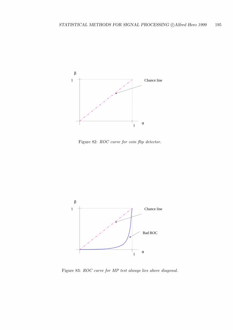
STATISTICAL METHODS FOR SIGNAL PROCESSING c©Alfred Hero 1999 195
1
1α
β
Chance line
Figure 82: ROC curve for coin flip detector.
1
1α
β
Chance line
Bad ROC
Figure 83: ROC curve for MP test always lies above diagonal.
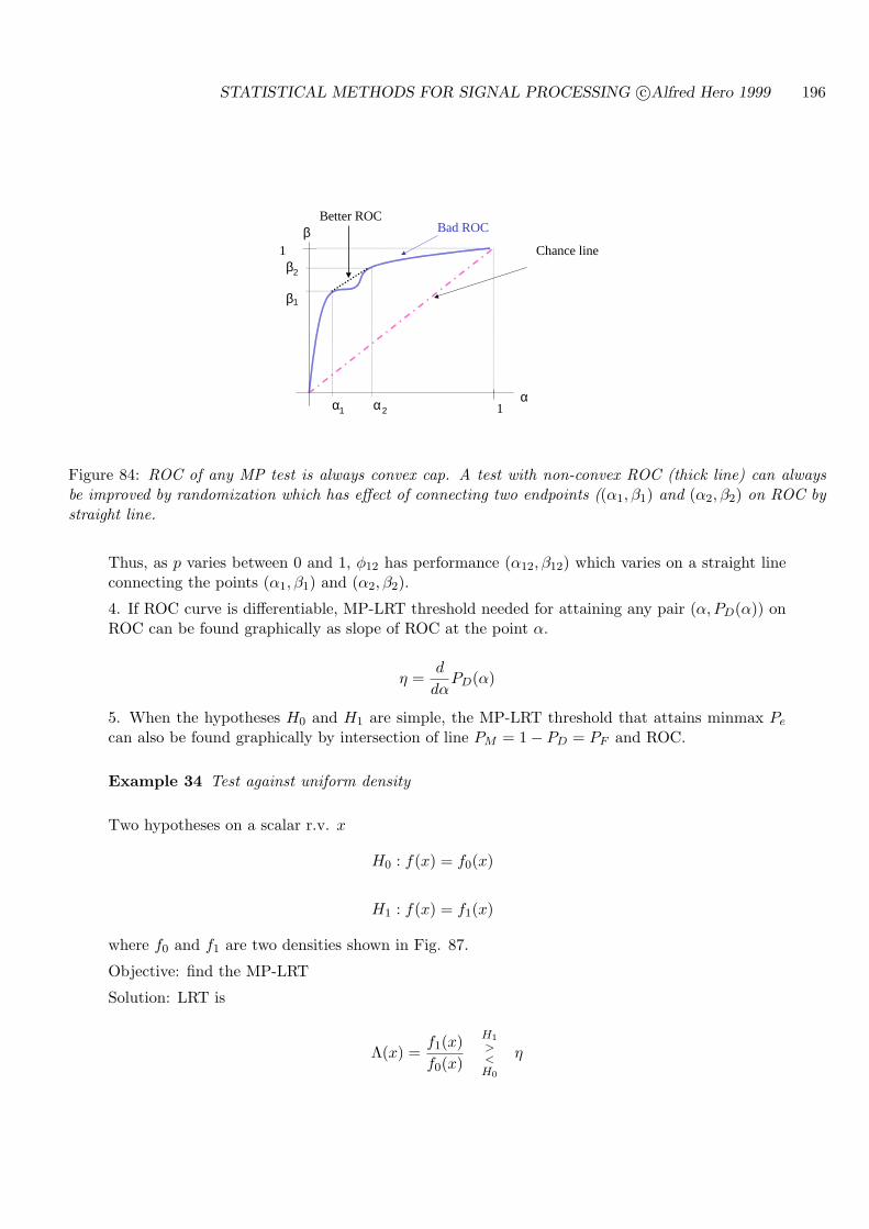
STATISTICAL METHODS FOR SIGNAL PROCESSING c©Alfred Hero 1999 196
1
1α
βChance line
Bad ROCBetter ROC
α α
β
β1
1
2
2
Figure 84: ROC of any MP test is always convex cap. A test with non-convex ROC (thick line) can alwaysbe improved by randomization which has effect of connecting two endpoints ((α1, β1) and (α2, β2) on ROC bystraight line.
Thus, as p varies between 0 and 1, φ12 has performance (α12, β12) which varies on a straight lineconnecting the points (α1, β1) and (α2, β2).
4. If ROC curve is differentiable, MP-LRT threshold needed for attaining any pair (α, PD(α)) onROC can be found graphically as slope of ROC at the point α.
η =d
dαPD(α)
5. When the hypotheses H0 and H1 are simple, the MP-LRT threshold that attains minmax Pe
can also be found graphically by intersection of line PM = 1− PD = PF and ROC.
Example 34 Test against uniform density
Two hypotheses on a scalar r.v. x
H0 : f(x) = f0(x)
H1 : f(x) = f1(x)
where f0 and f1 are two densities shown in Fig. 87.
Objective: find the MP-LRT
Solution: LRT is
Λ(x) =f1(x)f0(x)
H1
><H0
η
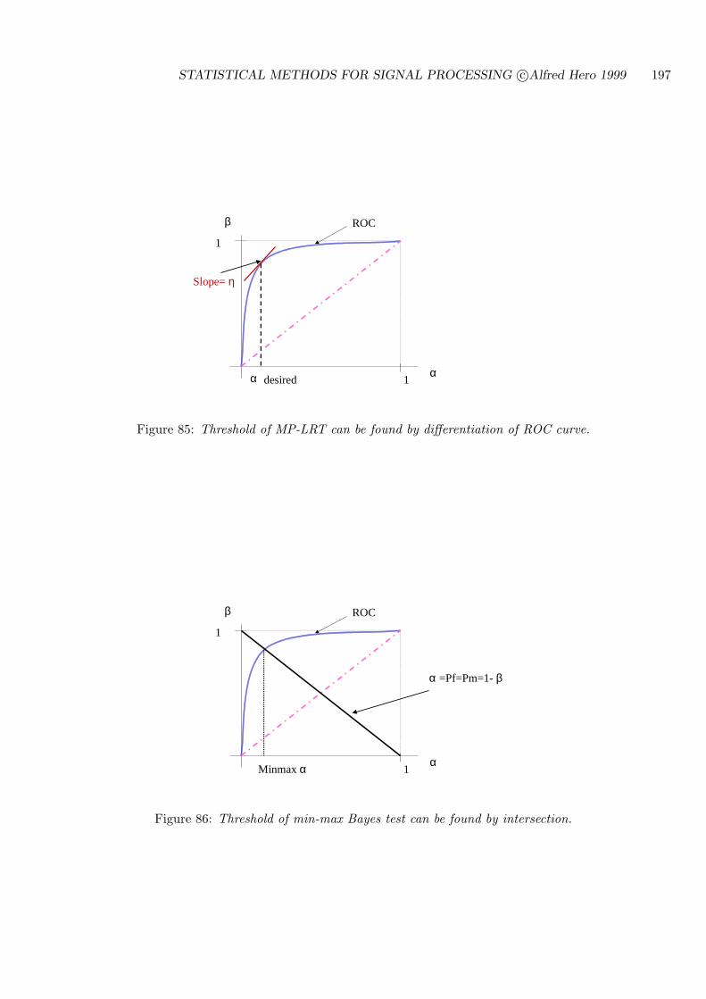
STATISTICAL METHODS FOR SIGNAL PROCESSING c©Alfred Hero 1999 197
1
1α
β ROC
Slope= η
α desired
Figure 85: Threshold of MP-LRT can be found by differentiation of ROC curve.
1
1α
β ROC
α =Pf=Pm=1- β
Minmax α
Figure 86: Threshold of min-max Bayes test can be found by intersection.
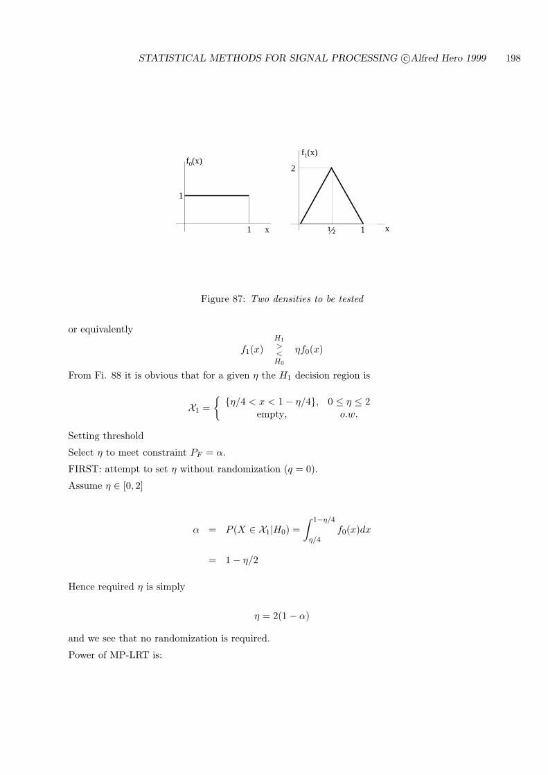
STATISTICAL METHODS FOR SIGNAL PROCESSING c©Alfred Hero 1999 198
1
1 x x
2
1½
f0(x)f1(x)
Figure 87: Two densities to be tested
or equivalently
f1(x)H1
><H0
ηf0(x)
From Fi. 88 it is obvious that for a given η the H1 decision region is
X1 = η/4 < x < 1− η/4, 0 ≤ η ≤ 2
empty, o.w.
Setting threshold
Select η to meet constraint PF = α.
FIRST: attempt to set η without randomization (q = 0).
Assume η ∈ [0, 2]
α = P (X ∈ X1|H0) =∫ 1−η/4
η/4f0(x)dx
= 1− η/2
Hence required η is simply
η = 2(1− α)
and we see that no randomization is required.
Power of MP-LRT is:
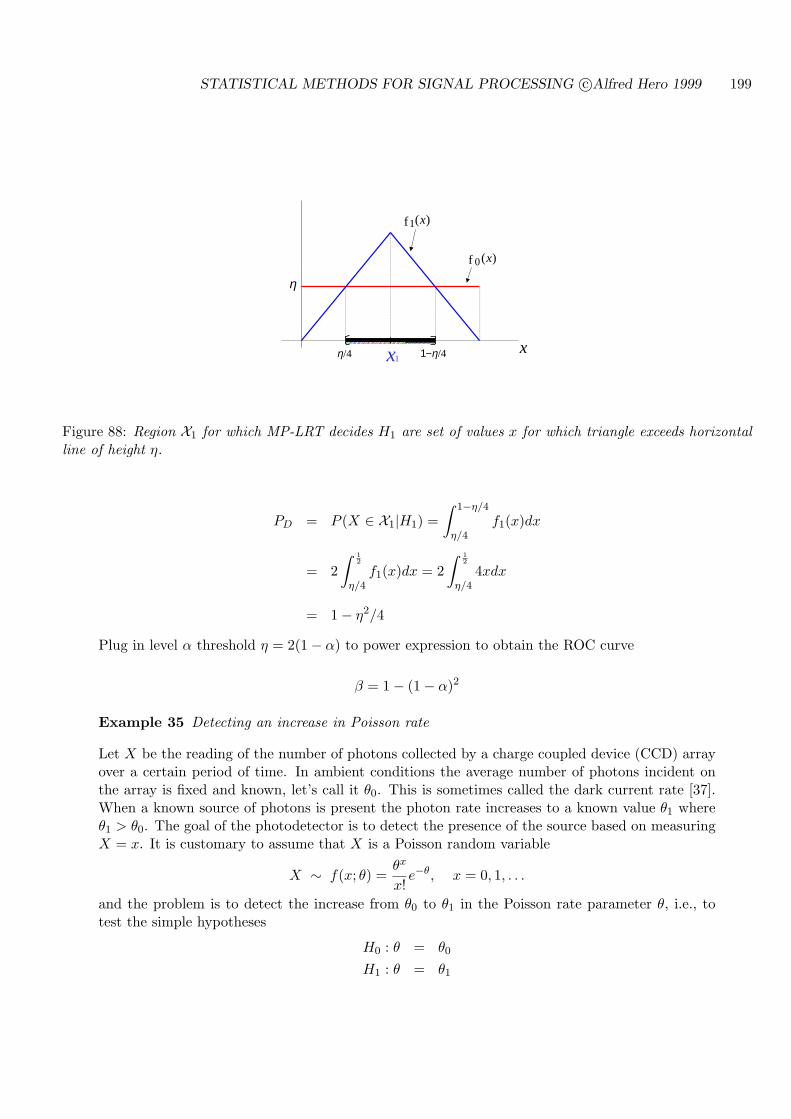
STATISTICAL METHODS FOR SIGNAL PROCESSING c©Alfred Hero 1999 199
η
η/4 1−η/4
)(f1 x
)(f 0 x
x1x
Figure 88: Region X1 for which MP-LRT decides H1 are set of values x for which triangle exceeds horizontalline of height η.
PD = P (X ∈ X1|H1) =∫ 1−η/4
η/4f1(x)dx
= 2∫ 1
2
η/4f1(x)dx = 2
∫ 12
η/44xdx
= 1− η2/4
Plug in level α threshold η = 2(1− α) to power expression to obtain the ROC curve
β = 1− (1− α)2
Example 35 Detecting an increase in Poisson rate
Let X be the reading of the number of photons collected by a charge coupled device (CCD) arrayover a certain period of time. In ambient conditions the average number of photons incident onthe array is fixed and known, let’s call it θ0. This is sometimes called the dark current rate [37].When a known source of photons is present the photon rate increases to a known value θ1 whereθ1 > θ0. The goal of the photodetector is to detect the presence of the source based on measuringX = x. It is customary to assume that X is a Poisson random variable
X ∼ f(x; θ) =θx
x!e−θ, x = 0, 1, . . .
and the problem is to detect the increase from θ0 to θ1 in the Poisson rate parameter θ, i.e., totest the simple hypotheses
H0 : θ = θ0
H1 : θ = θ1
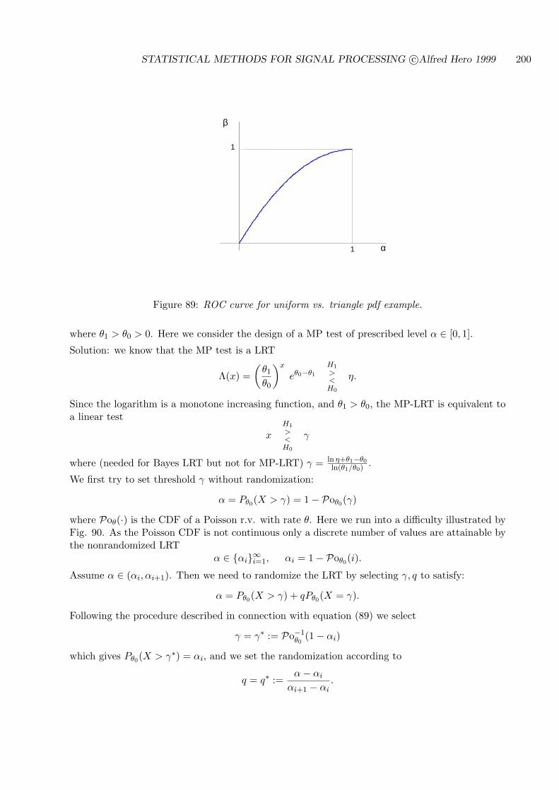
STATISTICAL METHODS FOR SIGNAL PROCESSING c©Alfred Hero 1999 200
1
1
α
β
Figure 89: ROC curve for uniform vs. triangle pdf example.
where θ1 > θ0 > 0. Here we consider the design of a MP test of prescribed level α ∈ [0, 1].
Solution: we know that the MP test is a LRT
Λ(x) =(
θ1
θ0
)x
eθ0−θ1
H1
><H0
η.
Since the logarithm is a monotone increasing function, and θ1 > θ0, the MP-LRT is equivalent toa linear test
xH1
><H0
γ
where (needed for Bayes LRT but not for MP-LRT) γ = ln η+θ1−θ0
ln(θ1/θ0) .
We first try to set threshold γ without randomization:
α = Pθ0(X > γ) = 1− Poθ0(γ)
where Poθ(·) is the CDF of a Poisson r.v. with rate θ. Here we run into a difficulty illustrated byFig. 90. As the Poisson CDF is not continuous only a discrete number of values are attainable bythe nonrandomized LRT
α ∈ αi∞i=1, αi = 1− Poθ0(i).
Assume α ∈ (αi, αi+1). Then we need to randomize the LRT by selecting γ, q to satisfy:
α = Pθ0(X > γ) + qPθ0(X = γ).
Following the procedure described in connection with equation (89) we select
γ = γ∗ := Po−1θ0
(1− αi)
which gives Pθ0(X > γ∗) = αi, and we set the randomization according to
q = q∗ :=α− αi
αi+1 − αi.
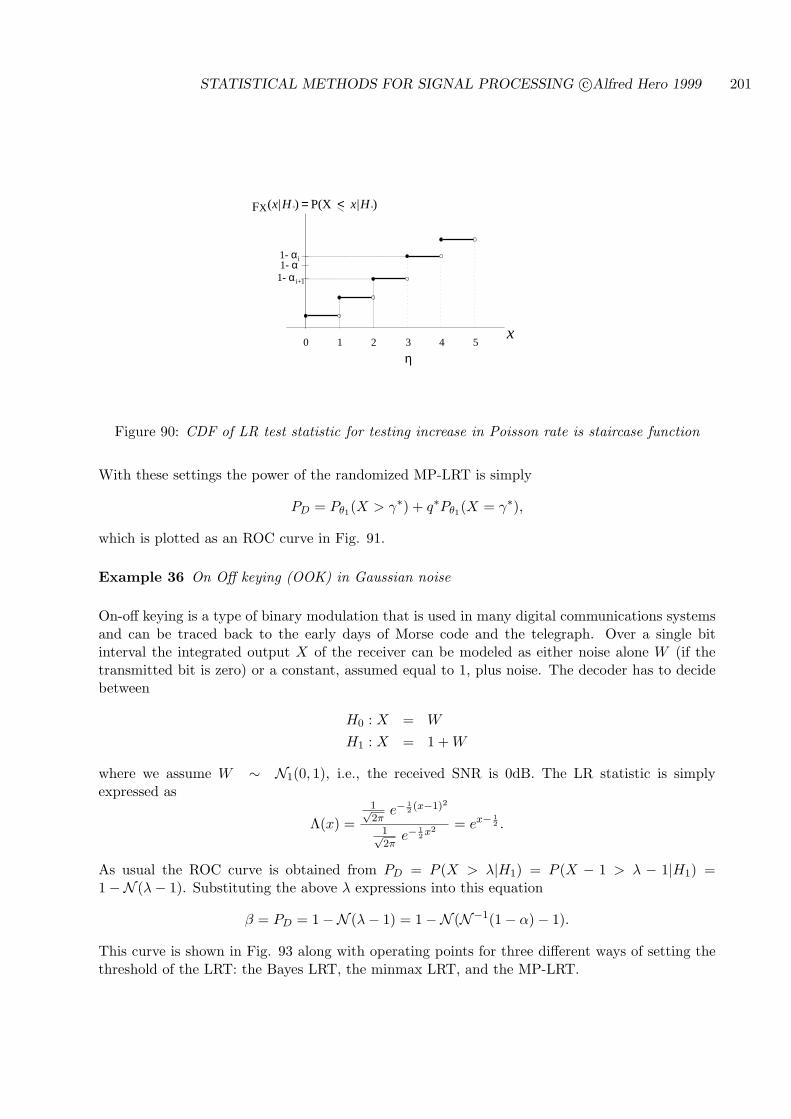
STATISTICAL METHODS FOR SIGNAL PROCESSING c©Alfred Hero 1999 201
1 2 0 3 4 5
1- αi1- α
1- αi+1
)| P(X )|(F 00X HxHx <=
x
η
Figure 90: CDF of LR test statistic for testing increase in Poisson rate is staircase function
With these settings the power of the randomized MP-LRT is simply
PD = Pθ1(X > γ∗) + q∗Pθ1(X = γ∗),
which is plotted as an ROC curve in Fig. 91.
Example 36 On Off keying (OOK) in Gaussian noise
On-off keying is a type of binary modulation that is used in many digital communications systemsand can be traced back to the early days of Morse code and the telegraph. Over a single bitinterval the integrated output X of the receiver can be modeled as either noise alone W (if thetransmitted bit is zero) or a constant, assumed equal to 1, plus noise. The decoder has to decidebetween
H0 : X = W
H1 : X = 1 + W
where we assume W ∼ N1(0, 1), i.e., the received SNR is 0dB. The LR statistic is simplyexpressed as
Λ(x) =1√2π
e− 12 (x−1)2
1√2π
e− 12x2 = ex− 1
2 .
As usual the ROC curve is obtained from PD = P (X > λ|H1) = P (X − 1 > λ − 1|H1) =1−N (λ− 1). Substituting the above λ expressions into this equation
β = PD = 1−N (λ− 1) = 1−N (N−1(1− α)− 1).
This curve is shown in Fig. 93 along with operating points for three different ways of setting thethreshold of the LRT: the Bayes LRT, the minmax LRT, and the MP-LRT.
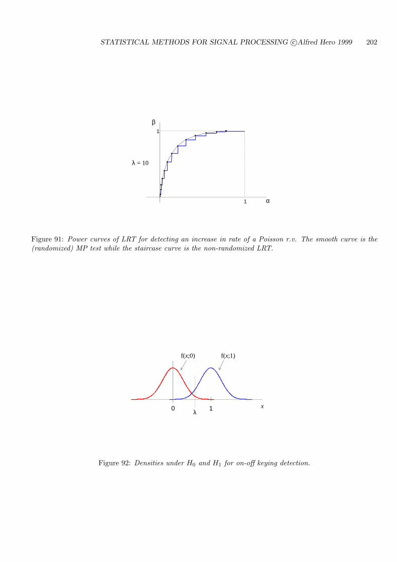
STATISTICAL METHODS FOR SIGNAL PROCESSING c©Alfred Hero 1999 202
1
1
α
β
λ = 10
Figure 91: Power curves of LRT for detecting an increase in rate of a Poisson r.v. The smooth curve is the(randomized) MP test while the staircase curve is the non-randomized LRT.
0 1λ
f(x;0) f(x;1)
x
Figure 92: Densities under H0 and H1 for on-off keying detection.
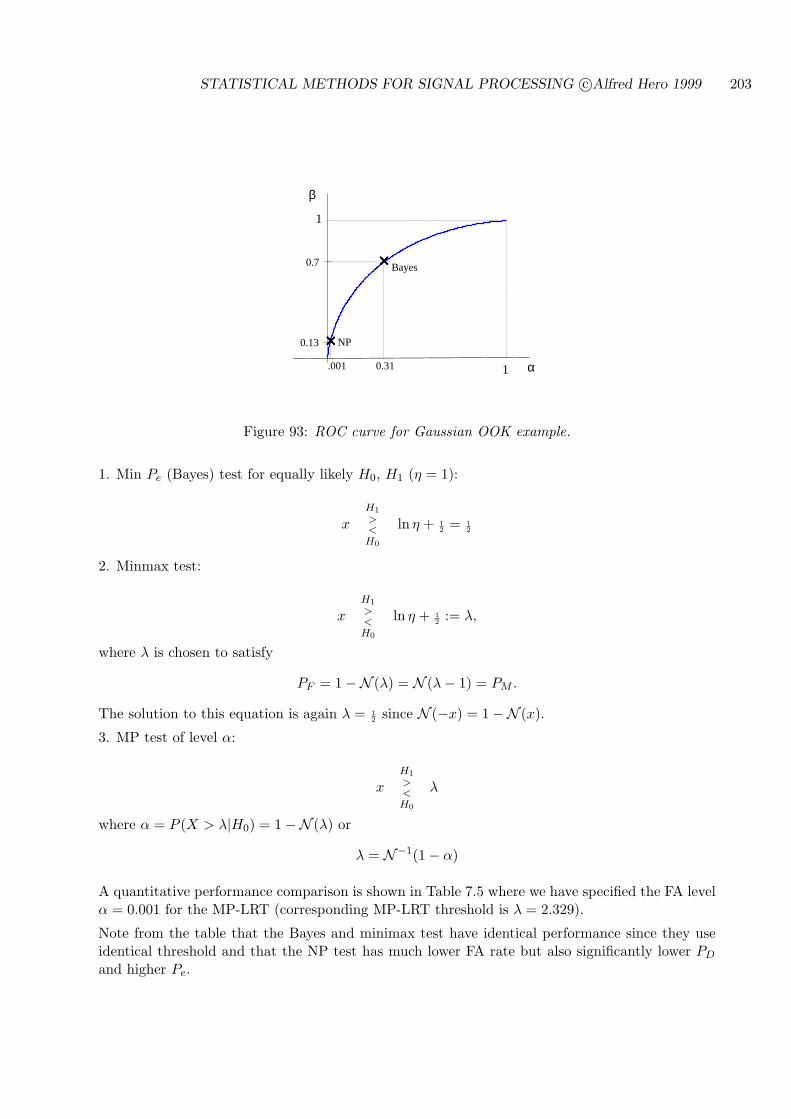
STATISTICAL METHODS FOR SIGNAL PROCESSING c©Alfred Hero 1999 203
××××
0.31.001
Bayes
NP××××
β
α
1
1
0.7
0.13
Figure 93: ROC curve for Gaussian OOK example.
1. Min Pe (Bayes) test for equally likely H0, H1 (η = 1):
xH1
><H0
ln η + 12 = 1
2
2. Minmax test:
xH1
><H0
ln η + 12 := λ,
where λ is chosen to satisfy
PF = 1−N (λ) = N (λ− 1) = PM .
The solution to this equation is again λ = 12 since N (−x) = 1−N (x).
3. MP test of level α:
xH1
><H0
λ
where α = P (X > λ|H0) = 1−N (λ) or
λ = N−1(1− α)
A quantitative performance comparison is shown in Table 7.5 where we have specified the FA levelα = 0.001 for the MP-LRT (corresponding MP-LRT threshold is λ = 2.329).
Note from the table that the Bayes and minimax test have identical performance since they useidentical threshold and that the NP test has much lower FA rate but also significantly lower PD
and higher Pe.
STATISTICAL METHODS FOR SIGNAL PROCESSING c©Alfred Hero 1999 204
PF PD Pe
Bayes 0.31 0.69 0.31Minmax 0.31 0.69 0.31NP 0.001 0.092 0.5
Table 1: Performance comparisons for three different threshold settings in OOK example.
7.6 BACKGROUND AND REFERENCES
There are many good textbooks on detection theory for signal processing, control and communi-cations. The books by Van Trees [72] and Whalen [75] are classics in the field. One of the earliestrelevant reference books covering signal detection theory is Middleton’s statistical communica-tions theory opus [45] which adopts a mathematical-physics perspective. The more recent bookby Helstrom [25] takes a similar but more engineering-oriented perspective. Another recent bookwith a signal processing focus on signal detection is Srinath, Rajasekaran and Viswanathan [66].For a somewhat more advanced mathematical treatment the reader may wish to consult the bookby Poor [54]. The above books concentrate on continuous time measurements which we do notcover in this chapter. The book by Mood, Graybill and Boes [47] has a very nice but elementarytreatment of the statistical methodology. More advanced treatments are found in books by Bickeland Doksum [7], Lehmann [38] and Ferguson [16].
7.7 EXERCISES
7.1 A proprietary binary hypothesis test φ is implemented in a software package which you areconsidering purchasing based on a trial examination period. You run several experiments andobtain the following table of probabilities of detection β vs. false alarm α
α β0.1 0.20.3 0.40.5 0.80.7 0.9
Comment on the quality of this test. Could you improve on this test? If so specify theimproved test and compute its ROC curve.
7.2 Let Z be a random variable with values in the interval [−1, 1] having density function
pθ(z) =12
33 + θ
(θz2 + 1
)
where θ > 0. Note θ controls the deviation of pθ from the uniform density p0. You are totest Z against non-uniformity given a single sample Z.
(a) Assuming priors p = P (H1) = 1− P (H0) (note this is opposite to the convention of thischapter) derive the minimum probability of error (MAP) test for the simple hypothesesH0 : θ = 0 vs. H1 : θ = θ1, where θ1 is a fixed and known positive value.
(b) Find an expression for the ROC curve and plot for θ1 = 0, 1, 10.(c) Now find the form of the min-max test. Show how you can use your answer to part b)
to graphically determine the min-max threshold.(d) Derive the MP test for the same simple hypotheses as in part (a).
STATISTICAL METHODS FOR SIGNAL PROCESSING c©Alfred Hero 1999 205
7.3 Let Z be a single observation having density function
pθ(z) = (2θz + 1− θ), 0 ≤ z ≤ 1
where −1 ≤ θ ≤ 1.
(a) Find the most powerful test between the hypotheses
H0 : θ = 0H1 : θ = 1
Be sure to express your test in terms of the false alarm level α ∈ [0, 1]. Plot the ROCcurve for this test.
(b) repeat part (a) for H1 : θ = −1.
7.4 It is desired to test the following hypotheses based on a single sample x:
H0 : x ∼ f0(x) =32
x2,−1 ≤ x ≤ 1
H1 : x ∼ f1(x) =34
(1− x2),−1 ≤ x ≤ 1
(a) Under the assumption that the prior probabilities of H0 and H1 are identical, find theminimum probability of error (Bayes) test.
(b) Find the Most Powerful test of level α ∈ [0, 1].(c) Derive and plot the ROC curve for these tests.
7.5 Let f(x|H0) and f(x|H1) be densities of an observed r.v. x and assume that the likelihoodratio Λ = f(x|H1)/f(x|H0) has corresponding densities fΛ(λ|H0) and fΛ(λ|H1) under H0
and H1, respectively. Show that the slope dβ/dα at a point α of the ROC of the LRT is equalto the threshold η attaining level α. (Hint: show that dβ/dα = fΛ(η|H1)/fΛ(η|H0) and thenapply fΛ(u|Hk) =
∫x:Λ(x)=u f(x|Hk)dx, k = 0, 1.)
7.6 Let a detector have the ROC curve (α, β) : α ∈ [0, 1] where the power function β = β(α)is a function of the false alarm level α. The area under the ROC is defined as
AUC =∫ 1
0β(α)dα
The AUC is frequently used as an alternative to the power function to assess the performanceof various detectors. Assume simple hypotheses and invoke properties of ROCs in answeringthe following questions.
(a) Show that among all tests the MP LRT maximizes AUC.(b) Show the following inequalities for the AUC of a MP LRT
12≤ AUC ≤ β( 1
2) ≤ 1
(c) Show that for any LRT whose ROC β(α) is differentiable in α
AUC = 1−∫ 1
0αη(α)dα
where η = η(α) is the LRT’s threshold attaining the false alarm level α. When com-bined with (b) this implies the interesting result for LRT’s: as the integral is boundedlimα→0(αη) = 0, i.e. α decreases to zero faster than η(α) increases to ∞.

STATISTICAL METHODS FOR SIGNAL PROCESSING c©Alfred Hero 1999 206
7.7 Available is a single random sample X from density fθ(x), where θ ∈ 0, 1 and
f1(x) =1√2π
exp(−x2/2)
f0(x) =12
exp(−|x|).
You are to develop tests for the hypotheses
H0 : θ = 0H1 : θ = 1
(a) Derive the (non-randomized) likelihood ratio test (LRT) and the induced decision regionX1=x : decide H1 for given threshold η. Draw the decision region as a function of thethreshold, i.e. plot the region X1 for several values of η > 0.
(b) Compute the false alarm probability PF and the detection probability PD of the test.Find an equation for and plot the ROC curve.
(c) Find the optimal Bayes test when H0 and H1 have prior probabilities P (H0) = 1/4 andP (H1) = 3/4, the cost of correct decisions is zero and the cost of incorrect decisions isone. What is PF and PD for this test?
(d) Find the optimal minimax test for unknown P (H0), P (H1). What is PF and PD for thistest?
(e) Find the Most Powerful test of level α = 0.2. What is PF and PD for this test?
End of chapter
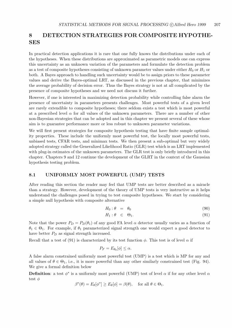
STATISTICAL METHODS FOR SIGNAL PROCESSING c©Alfred Hero 1999 207
8 DETECTION STRATEGIES FOR COMPOSITE HYPOTHE-SES
In practical detection applications it is rare that one fully knows the distributions under each ofthe hypotheses. When these distributions are approximated as parametric models one can expressthis uncertainty as an unknown variation of the parameters and formulate the detection problemas a test of composite hypotheses consisting of unknown parameter values under either H0 or H1 orboth. A Bayes approach to handling such uncertainty would be to assign priors to these parametervalues and derive the Bayes-optimal LRT, as discussed in the previous chapter, that minimizesthe average probability of decision error. Thus the Bayes strategy is not at all complicated by thepresence of composite hypotheses and we need not discuss it further.
However, if one is interested in maximizing detection probability while controlling false alarm thepresence of uncertainty in parameters presents challenges. Most powerful tests of a given levelare rarely extendible to composite hypotheses; there seldom exists a test which is most powerfulat a prescribed level α for all values of the unknown parameters. There are a number of othernon-Bayesian strategies that can be adopted and in this chapter we present several of these whoseaim is to guarantee performance more or less robust to unknown parameter variations.
We will first present strategies for composite hypothesis testing that have finite sample optimal-ity properties. These include the uniformly most powerful test, the locally most powerful tests,unbiased tests, CFAR tests, and minimax tests. We then present a sub-optimal but very widelyadopted strategy called the Generalized Likelihood Ratio (GLR) test which is an LRT implementedwith plug-in estimates of the unknown parameters. The GLR test is only briefly introduced in thischapter. Chapters 9 and 12 continue the development of the GLRT in the context of the Gaussianhypothesis testing problem.
8.1 UNIFORMLY MOST POWERFUL (UMP) TESTS
After reading this section the reader may feel that UMP tests are better described as a miraclethan a strategy. However, development of the theory of UMP tests is very instructive as it helpsunderstand the challenges posed in trying to test composite hypotheses. We start by consideringa simple null hypothesis with composite alternative
H0 : θ = θ0 (90)H1 : θ ∈ Θ1. (91)
Note that the power PD = PD(θ1) of any good FA level α detector usually varies as a function ofθ1 ∈ Θ1. For example, if θ1 parameterized signal strength one would expect a good detector tohave better PD as signal strength increased.
Recall that a test of (91) is characterized by its test function φ. This test is of level α if
PF = Eθ0 [φ] ≤ α.
A false alarm constrained uniformly most powerful test (UMP) is a test which is MP for any andall values of θ ∈ Θ1, i.e., it is more powerful than any other similarly constrained test (Fig. 94).We give a formal definition below
Definition: a test φ∗ is a uniformly most powerful (UMP) test of level α if for any other level αtest φ
β∗(θ) = Eθ[φ∗] ≥ Eθ[φ] = β(θ), for all θ ∈ Θ1.
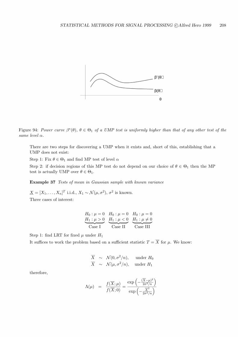
STATISTICAL METHODS FOR SIGNAL PROCESSING c©Alfred Hero 1999 208
θ
β(θ)
β∗(θ)
Figure 94: Power curve β∗(θ), θ ∈ Θ1 of a UMP test is uniformly higher than that of any other test of thesame level α.
There are two steps for discovering a UMP when it exists and, short of this, establishing that aUMP does not exist:
Step 1: Fix θ ∈ Θ1 and find MP test of level α
Step 2: if decision regions of this MP test do not depend on our choice of θ ∈ Θ1 then the MPtest is actually UMP over θ ∈ Θ1.
Example 37 Tests of mean in Gaussian sample with known variance
X = [X1, . . . , Xn]T i.i.d., X1 ∼ N (µ, σ2), σ2 is known.
Three cases of interest:
H0 : µ = 0 H0 : µ = 0 H0 : µ = 0H1 : µ > 0︸ ︷︷ ︸
Case I
H1 : µ < 0︸ ︷︷ ︸Case II
H1 : µ 6= 0︸ ︷︷ ︸Case III
Step 1: find LRT for fixed µ under H1
It suffices to work the problem based on a sufficient statistic T = X for µ. We know:
X ∼ N (0, σ2/n), under H0
X ∼ N (µ, σ2/n), under H1
therefore,
Λ(µ) =f(X;µ)f(X; 0)
=exp
(− (X−µ)2
2σ2/n
)
exp(− X
2
2σ2/n
)

STATISTICAL METHODS FOR SIGNAL PROCESSING c©Alfred Hero 1999 209
= exp(
nµ
σ2X − nµ2
2σ2
) H1
><H0
η
For clarity, our notation explicitly brings out the dependance of the likelihood ratio on µ. Notethat Λ(µ) is monotone increasing in µX so that one form of the MP-LRT is
µ
(√n X
σ
) H1
><H0
γ
CASE I: Single sided alternative H1 : µ > 0
In this case µ can be absorbed into RHS without changing inequalities:
T (X) =√
n X
σ
H1
><H0
γ+
or equivalently, MP-LRT is the linear detector
n∑
i=1
Xi
H1
><H0
γ′= γ+ √n σ2
Ho
H1
> <
xkγΣ
Figure 95: Optimal detector for positive Gaussian mean is a memoryless linear device followed by a summerand decision mechanism.
Next we must set threshold:
Since we know X ∼ N (0, σ2/n) under H0:
α = P0(√
n X/σ︸ ︷︷ ︸N (0,1)
> γ+) = 1−N (γ+)
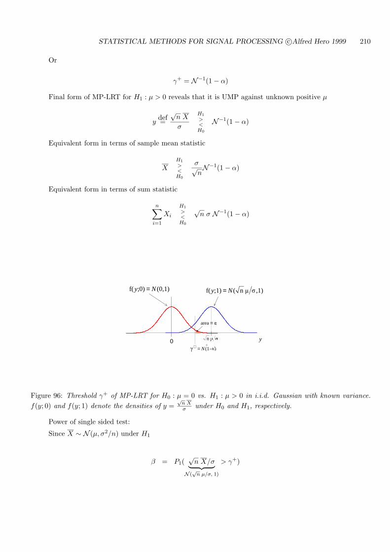
STATISTICAL METHODS FOR SIGNAL PROCESSING c©Alfred Hero 1999 210
Or
γ+ = N−1(1− α)
Final form of MP-LRT for H1 : µ > 0 reveals that it is UMP against unknown positive µ
ydef=
√n X
σ
H1
><H0
N−1(1− α)
Equivalent form in terms of sample mean statistic
XH1
><H0
σ√nN−1(1− α)
Equivalent form in terms of sum statistic
n∑
i=1
Xi
H1
><H0
√n σ N−1(1− α)
0 y1 n
.-(1 N=+
.area =
-1
,1)1 n( ;1)f( Ny =(0,1) ;0)f( Ny =
Figure 96: Threshold γ+ of MP-LRT for H0 : µ = 0 vs. H1 : µ > 0 in i.i.d. Gaussian with known variance.f(y; 0) and f(y; 1) denote the densities of y =
√n Xσ under H0 and H1, respectively.
Power of single sided test:
Since X ∼ N (µ, σ2/n) under H1
β = P1(√
n X/σ︸ ︷︷ ︸N (√
n µ/σ, 1)
> γ+)
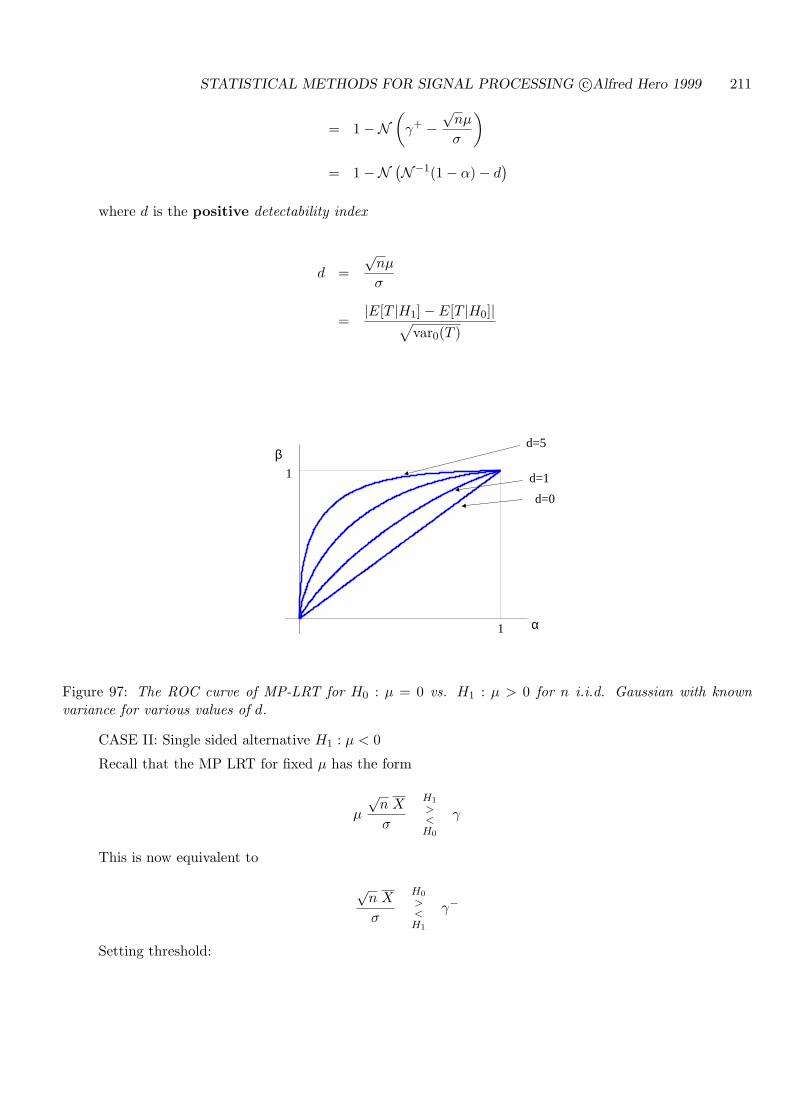
STATISTICAL METHODS FOR SIGNAL PROCESSING c©Alfred Hero 1999 211
= 1−N(
γ+ −√
nµ
σ
)
= 1−N (N−1(1− α)− d)
where d is the positive detectability index
d =√
nµ
σ
=|E[T |H1]− E[T |H0]|√
var0(T )
1
1
β
α
d=0
d=1
d=5
Figure 97: The ROC curve of MP-LRT for H0 : µ = 0 vs. H1 : µ > 0 for n i.i.d. Gaussian with knownvariance for various values of d.
CASE II: Single sided alternative H1 : µ < 0
Recall that the MP LRT for fixed µ has the form
µ
√n X
σ
H1
><H0
γ
This is now equivalent to
√n X
σ
H0
><H1
γ−
Setting threshold:
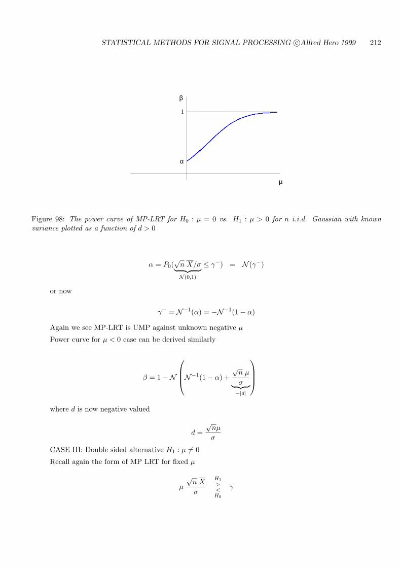
STATISTICAL METHODS FOR SIGNAL PROCESSING c©Alfred Hero 1999 212
1
µ
α
β
Figure 98: The power curve of MP-LRT for H0 : µ = 0 vs. H1 : µ > 0 for n i.i.d. Gaussian with knownvariance plotted as a function of d > 0
α = P0(√
n X/σ︸ ︷︷ ︸N (0,1)
≤ γ−) = N (γ−)
or now
γ− = N−1(α) = −N−1(1− α)
Again we see MP-LRT is UMP against unknown negative µ
Power curve for µ < 0 case can be derived similarly
β = 1−N
N−1(1− α) +
√n µ
σ︸ ︷︷ ︸−|d|
where d is now negative valued
d =√
nµ
σ
CASE III: Double sided alternative H1 : µ 6= 0
Recall again the form of MP LRT for fixed µ
µ
√n X
σ
H1
><H0
γ
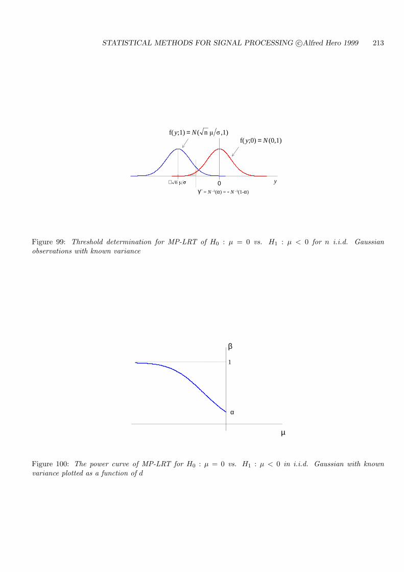
STATISTICAL METHODS FOR SIGNAL PROCESSING c©Alfred Hero 1999 213
0 y
,1)1 n( ;1)f( Ny =(0,1) ;0)f( Ny =
1 n+
= N -1(α) = - N -1(1-α)γ−
Figure 99: Threshold determination for MP-LRT of H0 : µ = 0 vs. H1 : µ < 0 for n i.i.d. Gaussianobservations with known variance
1
µ
α
β
Figure 100: The power curve of MP-LRT for H0 : µ = 0 vs. H1 : µ < 0 in i.i.d. Gaussian with knownvariance plotted as a function of d
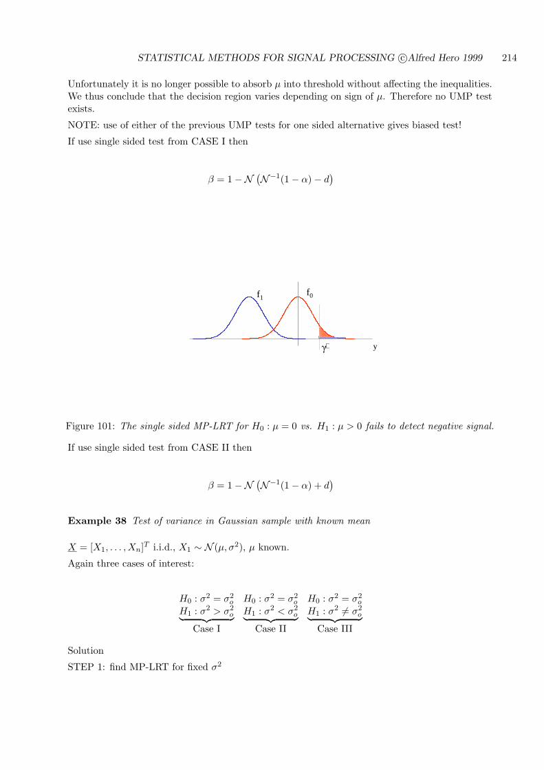
STATISTICAL METHODS FOR SIGNAL PROCESSING c©Alfred Hero 1999 214
Unfortunately it is no longer possible to absorb µ into threshold without affecting the inequalities.We thus conclude that the decision region varies depending on sign of µ. Therefore no UMP testexists.
NOTE: use of either of the previous UMP tests for one sided alternative gives biased test!
If use single sided test from CASE I then
β = 1−N (N−1(1− α)− d)
+
f0f1
y
Figure 101: The single sided MP-LRT for H0 : µ = 0 vs. H1 : µ > 0 fails to detect negative signal.
If use single sided test from CASE II then
β = 1−N (N−1(1− α) + d)
Example 38 Test of variance in Gaussian sample with known mean
X = [X1, . . . , Xn]T i.i.d., X1 ∼ N (µ, σ2), µ known.
Again three cases of interest:
H0 : σ2 = σ2o H0 : σ2 = σ2
o H0 : σ2 = σ2o
H1 : σ2 > σ2o︸ ︷︷ ︸
Case I
H1 : σ2 < σ2o︸ ︷︷ ︸
Case II
H1 : σ2 6= σ2o︸ ︷︷ ︸
Case III
Solution
STEP 1: find MP-LRT for fixed σ2
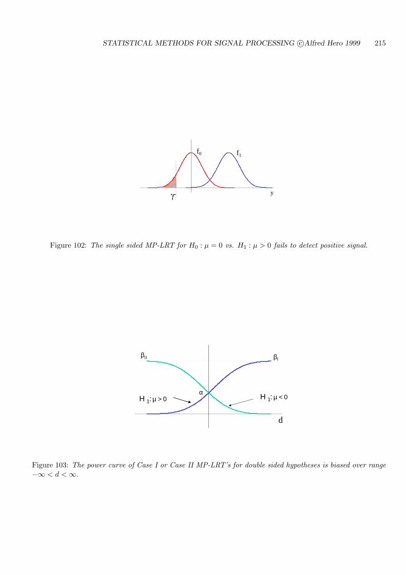
STATISTICAL METHODS FOR SIGNAL PROCESSING c©Alfred Hero 1999 215
−
f0 f1
y
Figure 102: The single sided MP-LRT for H0 : µ = 0 vs. H1 : µ > 0 fails to detect positive signal.
d
βΙΙ βΙ
α Η 1: µ < 0 Η 1: µ > 0
Figure 103: The power curve of Case I or Case II MP-LRT’s for double sided hypotheses is biased over range−∞ < d < ∞.
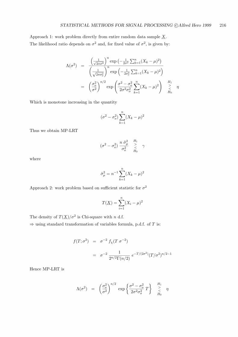
STATISTICAL METHODS FOR SIGNAL PROCESSING c©Alfred Hero 1999 216
Approach 1: work problem directly from entire random data sample X.
The likelihood ratio depends on σ2 and, for fixed value of σ2, is given by:
Λ(σ2) =
(1√
2πσ2
)nexp
(− 12σ2
∑nk=1(Xk − µ)2
)(
1√2πσ2
o
)n
exp(− 1
2σ2o
∑nk=1(Xk − µ)2
)
=(
σ2o
σ2
)n/2
exp
(σ2 − σ2
o
2σ2σ2o
n∑
k=1
(Xk − µ)2)
H1
><H0
η
Which is monotone increasing in the quantity
(σ2 − σ2o)
n∑
k=1
(Xk − µ)2
Thus we obtain MP-LRT
(σ2 − σ2o)
n σ2µ
σ2o
H1
><H0
γ
where
σ2µ = n−1
n∑
k=1
(Xk − µ)2
Approach 2: work problem based on sufficient statistic for σ2
T (X) =n∑
i=1
(Xi − µ)2
The density of T (X)/σ2 is Chi-square with n d.f.
⇒ using standard transformation of variables formula, p.d.f. of T is:
f(T ; σ2) = σ−2 fχ(T σ−2)
= σ−2 12n/2Γ(n/2)
e−T/(2σ2)(T/σ2)n/2−1
Hence MP-LRT is
Λ(σ2) =(
σ2o
σ2
)n/2
exp
σ2 − σ2o
2σ2σ2o
T
H1
><H0
η
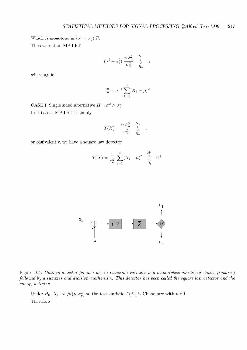
STATISTICAL METHODS FOR SIGNAL PROCESSING c©Alfred Hero 1999 217
Which is monotone in (σ2 − σ2o) T .
Thus we obtain MP-LRT
(σ2 − σ2o)
n σ2µ
σ2o
H1
><H0
γ
where again
σ2µ = n−1
n∑
k=1
(Xk − µ)2
CASE I: Single sided alternative H1 : σ2 > σ2o
In this case MP-LRT is simply
T (X) =n σ2
µ
σ2o
H1
><H0
γ+
or equivalently, we have a square law detector
T (X) =1σ2
o
n∑
i=1
(Xi − µ)2H1
><H0
γ+
Ho
H1
> <
xkγΣ
-
µ
( )2
Figure 104: Optimal detector for increase in Gaussian variance is a memoryless non-linear device (squarer)followed by a summer and decision mechanism. This detector has been called the square law detector and theenergy detector.
Under H0, Xk ∼ N (µ, σ2o) so the test statistic T (X) is Chi-square with n d.f.
Therefore

STATISTICAL METHODS FOR SIGNAL PROCESSING c©Alfred Hero 1999 218
α = P0(T (X) > γ+) = 1− χn(γ+)
and
γ+ = χ−1n (1− α)
Hence MP-LRT is
n σ2µ
σ2o
H1
><H0
χ−1n (1− α)
which is UMP against any σ2 > σ2o for known µ.
f(T;σ02)
f(T;σ2), σ2 >σ02
.-(11-n χ=+
T
Figure 105: Density functions under H0 and H1 of optimal UMP test statistic for testing against σ2 > σ2o for
known mean µ. Threshold γ+ is determined by the 1− α quantile of the H0 density.
Power: since σ2o
σ2
nσ2µ
σ2o
= χn
β = P1
(n σ2
µ/σ2o > γ+
)= 1− χn
(σ2
o
σ2χ−1
n (1− α))
CASE II: Single sided alternative H1 : σ2 < σ2o
Find that MP-LRT has form
n σ2µ
σ2o
H0
><H1
γ−
where now

STATISTICAL METHODS FOR SIGNAL PROCESSING c©Alfred Hero 1999 219
β
σ2/σ20
n = 3
0 1 2 3 4 5
0.2
0.3
0.5
0.7
0.9
1
α = 0.9α = 0.7α = 0.5 α = 0.3 α = 0.2
Figure 106: Power curves for one sided test of variance σ2 > σ2o for known mean µ with i.i.d. Gaussian
observations for various values of σ2/σ2o and n = 3.
0 0.2 0.4 0.6 0.8 10
0.2
0.4
0.6
0.8
1
RO C of Chi-square test σσσσ > σσσσ0
αααα
ββββ σσσσ2 /σσσσ
20=1
σσσσ2 /σσσσ
20=2
σσσσ2 /σσσσ
20=4
σσσσ2 /σσσσ
20=8
σσσσ2 /σσσσ
20=16
Figure 107: ROC curves for one sided test of variance σ2 > σ2o with i.i.d. Gaussian observations for various
values of σ2/σ2o and n = 3.
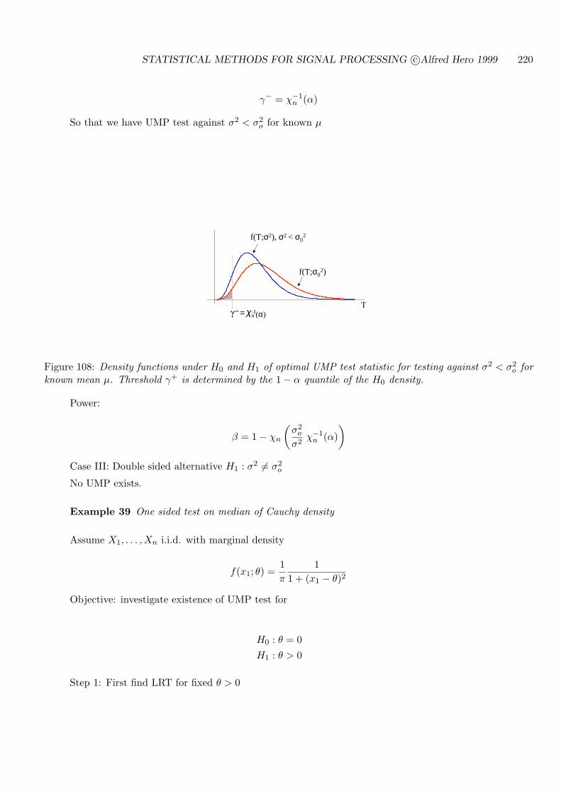
STATISTICAL METHODS FOR SIGNAL PROCESSING c©Alfred Hero 1999 220
γ− = χ−1n (α)
So that we have UMP test against σ2 < σ2o for known µ
f(T;σ02)
f(T;σ2), σ2 < σ02
1-n χ=− (α)
T
Figure 108: Density functions under H0 and H1 of optimal UMP test statistic for testing against σ2 < σ2o for
known mean µ. Threshold γ+ is determined by the 1− α quantile of the H0 density.
Power:
β = 1− χn
(σ2
o
σ2χ−1
n (α))
Case III: Double sided alternative H1 : σ2 6= σ2o
No UMP exists.
Example 39 One sided test on median of Cauchy density
Assume X1, . . . , Xn i.i.d. with marginal density
f(x1; θ) =1π
11 + (x1 − θ)2
Objective: investigate existence of UMP test for
H0 : θ = 0H1 : θ > 0
Step 1: First find LRT for fixed θ > 0
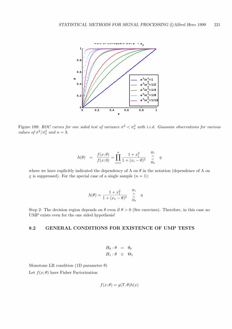
STATISTICAL METHODS FOR SIGNAL PROCESSING c©Alfred Hero 1999 221
0 0.2 0 .4 0 .6 0 .8 10
0.2
0 .4
0 .6
0 .8
1
R O C of C h i-square tes t σσσσ2 < σσσσ
2
0
αααα
ββββ σσσσ 2 /σσσσ 20= 1
σσσσ 2 /σσσσ 2
0= 1/2
σσσσ 2 /σσσσ 20= 1/4
σσσσ 2 /σσσσ 20= 1/8
σσσσ 2 /σσσσ 2
0= 1/16
Figure 109: ROC curves for one sided test of variance σ2 < σ2o with i.i.d. Gaussian observations for various
values of σ2/σ2o and n = 3.
Λ(θ) =f(x; θ)f(x; 0)
=n∏
i=1
1 + x2i
1 + (xi − θ)2
H1
><H0
η
where we have explicitly indicated the dependency of Λ on θ in the notation (dependence of Λ onx is suppressed). For the special case of a single sample (n = 1):
Λ(θ) =1 + x2
1
1 + (x1 − θ)2
H1
><H0
η
Step 2: The decision region depends on θ even if θ > 0 (See exercises). Therefore, in this case noUMP exists even for the one sided hypothesis!
8.2 GENERAL CONDITIONS FOR EXISTENCE OF UMP TESTS
H0 : θ = θ0
H1 : θ ∈ Θ1
Monotone LR condition (1D parameter θ)
Let f(x; θ) have Fisher Factorization
f(x; θ) = g(T, θ)h(x)
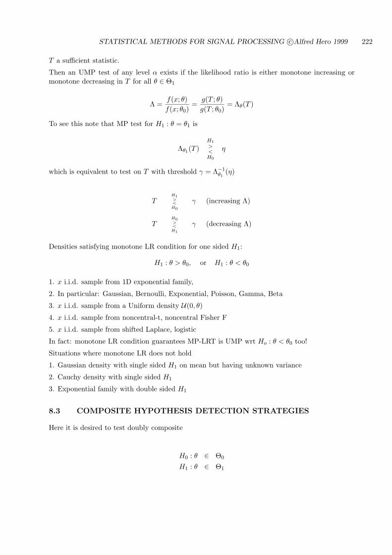
STATISTICAL METHODS FOR SIGNAL PROCESSING c©Alfred Hero 1999 222
T a sufficient statistic.
Then an UMP test of any level α exists if the likelihood ratio is either monotone increasing ormonotone decreasing in T for all θ ∈ Θ1
Λ =f(x; θ)f(x; θ0)
=g(T ; θ)g(T ; θ0)
= Λθ(T )
To see this note that MP test for H1 : θ = θ1 is
Λθ1(T )H1
><H0
η
which is equivalent to test on T with threshold γ = Λ−1θ1
(η)
TH1><
H0
γ (increasing Λ)
TH0><
H1
γ (decreasing Λ)
Densities satisfying monotone LR condition for one sided H1:
H1 : θ > θ0, or H1 : θ < θ0
1. x i.i.d. sample from 1D exponential family,
2. In particular: Gaussian, Bernoulli, Exponential, Poisson, Gamma, Beta
3. x i.i.d. sample from a Uniform density U(0, θ)
4. x i.i.d. sample from noncentral-t, noncentral Fisher F
5. x i.i.d. sample from shifted Laplace, logistic
In fact: monotone LR condition guarantees MP-LRT is UMP wrt Ho : θ < θ0 too!
Situations where monotone LR does not hold
1. Gaussian density with single sided H1 on mean but having unknown variance
2. Cauchy density with single sided H1
3. Exponential family with double sided H1
8.3 COMPOSITE HYPOTHESIS DETECTION STRATEGIES
Here it is desired to test doubly composite
H0 : θ ∈ Θ0
H1 : θ ∈ Θ1
STATISTICAL METHODS FOR SIGNAL PROCESSING c©Alfred Hero 1999 223
Now, most fixed detectors will have both PF and PD varying as functions of θ ∈ Θ0 and θ ∈ Θ1,respectively.
Recall that for composite H0 we say that test φ is of level α if
maxθ0∈Θ0
PF (θ0) ≤ α
where PF (θ) = Eθ0 [φ]
Two classes of strategies:
1. Optimize alternative detection criterion
2. Constrain form of detector to a class for which UMP may exist
8.4 MINIMAX TESTS
A conservative approach to testing composite hypotheses would be to maximize worst case powerunder a constraint on worst case false alarm. This approach is called a minimax strategy andleads to conservative but minimax optimal tests. Minimax approaches are not very widespread insignal processing applications due to their overly conservative performance and their often difficultimplementation.
Objective: find level α test which satisfies the constraint:
maxθ∈Θ0
Eθ[φ] ≤ α,
and maximizes the worst case powerminθ∈Θ1
Eθ[φ].
METHOD OF SOLUTION: find “least favorable” densities
Simplifying assumption: Θ discrete parameter space.
Fundamental identity on the mean [22]: For any summable sequence a(k)k and any probabilitydistribution p(k)k
mink
a(k) ≤∑
k
a(k)p(k) ≤ maxk
a(k)
with equality when p(k) = delta function concentrated on argminka(k) and argmaxka(k). There-fore
mink
a(k) = minp(k)
∑
k
a(k)p(k), maxk
a(k) = maxp(k)
∑
k
a(k)p(k)
* Let p0(θ) be an arbitrary probability distribution on Θ0
* Let p1(θ) be an arbitrary probability distribution on Θ1
Then the worst case PF (θ) and PM (θ) can be expressed as worst case average PF and PM
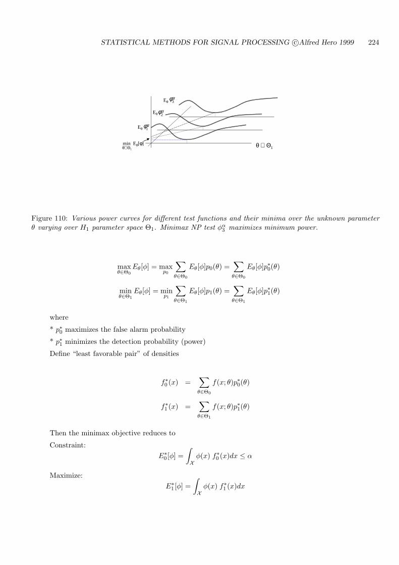
STATISTICAL METHODS FOR SIGNAL PROCESSING c©Alfred Hero 1999 224
αφ1
αφ2
αφ3
θ ∈ Θ1min Eθ[φ]θ∈Θ1
Eθ
Eθ
Eθ
Figure 110: Various power curves for different test functions and their minima over the unknown parameterθ varying over H1 parameter space Θ1. Minimax NP test φα
3 maximizes minimum power.
maxθ∈Θ0
Eθ[φ] = maxp0
∑
θ∈Θ0
Eθ[φ]p0(θ) =∑
θ∈Θ0
Eθ[φ]p∗0(θ)
minθ∈Θ1
Eθ[φ] = minp1
∑
θ∈Θ1
Eθ[φ]p1(θ) =∑
θ∈Θ1
Eθ[φ]p∗1(θ)
where
* p∗0 maximizes the false alarm probability
* p∗1 minimizes the detection probability (power)
Define “least favorable pair” of densities
f∗0 (x) =∑
θ∈Θ0
f(x; θ)p∗0(θ)
f∗1 (x) =∑
θ∈Θ1
f(x; θ)p∗1(θ)
Then the minimax objective reduces to
Constraint:E∗
0 [φ] =∫
Xφ(x) f∗0 (x)dx ≤ α
Maximize:E∗
1 [φ] =∫
Xφ(x) f∗1 (x)dx
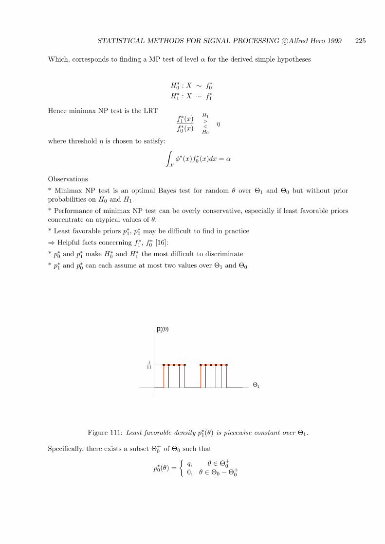
STATISTICAL METHODS FOR SIGNAL PROCESSING c©Alfred Hero 1999 225
Which, corresponds to finding a MP test of level α for the derived simple hypotheses
H∗0 : X ∼ f∗0
H∗1 : X ∼ f∗1
Hence minimax NP test is the LRTf∗1 (x)f∗0 (x)
H1
><H0
η
where threshold η is chosen to satisfy:∫
Xφ∗(x)f∗0 (x)dx = α
Observations
* Minimax NP test is an optimal Bayes test for random θ over Θ1 and Θ0 but without priorprobabilities on H0 and H1.
* Performance of minimax NP test can be overly conservative, especially if least favorable priorsconcentrate on atypical values of θ.
* Least favorable priors p∗1, p∗0 may be difficult to find in practice
⇒ Helpful facts concerning f∗1 , f∗0 [16]:
* p∗0 and p∗1 make H∗0 and H∗
1 the most difficult to discriminate
* p∗1 and p∗0 can each assume at most two values over Θ1 and Θ0
111
)(*1p
Θ1
Figure 111: Least favorable density p∗1(θ) is piecewise constant over Θ1.
Specifically, there exists a subset Θ+0 of Θ0 such that
p∗0(θ) =
q, θ ∈ Θ+0
0, θ ∈ Θ0 −Θ+0
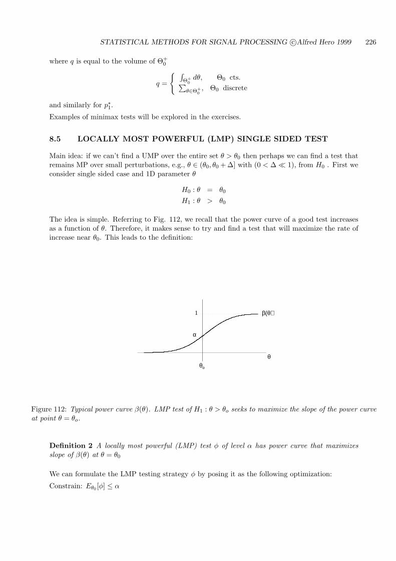
STATISTICAL METHODS FOR SIGNAL PROCESSING c©Alfred Hero 1999 226
where q is equal to the volume of Θ+0
q =
∫Θ+
0dθ, Θ0 cts.∑
θ∈Θ+0, Θ0 discrete
and similarly for p∗1.
Examples of minimax tests will be explored in the exercises.
8.5 LOCALLY MOST POWERFUL (LMP) SINGLE SIDED TEST
Main idea: if we can’t find a UMP over the entire set θ > θ0 then perhaps we can find a test thatremains MP over small perturbations, e.g., θ ∈ (θ0, θ0 + ∆] with (0 < ∆ ¿ 1), from H0 . First weconsider single sided case and 1D parameter θ
H0 : θ = θ0
H1 : θ > θ0
The idea is simple. Referring to Fig. 112, we recall that the power curve of a good test increasesas a function of θ. Therefore, it makes sense to try and find a test that will maximize the rate ofincrease near θ0. This leads to the definition:
β(θ)
α
θθο
1
Figure 112: Typical power curve β(θ). LMP test of H1 : θ > θo seeks to maximize the slope of the power curveat point θ = θo.
Definition 2 A locally most powerful (LMP) test φ of level α has power curve that maximizesslope of β(θ) at θ = θ0
We can formulate the LMP testing strategy φ by posing it as the following optimization:
Constrain: Eθ0 [φ] ≤ α

STATISTICAL METHODS FOR SIGNAL PROCESSING c©Alfred Hero 1999 227
Maximize: ddθ0
Eθ0 [φ]
Similarly to the derivation of NPL in the previous chapter, we obtain the solution φ to thisoptimization as the test
φLMP (x) =
1, df(x; θ0)/dθ0 > ηf(x; θ0)q, df(x; θ0)/dθ0 = ηf(x; θ0)0, df(x; θ0)/dθ0 < ηf(x; θ0)
Or for short
ΛLMP(x) =df(x; θ0)/dθ0
f(x; θ0)
H1
><H0
η
where η is selected to satisfy constraint (possibly with randomization)
Eθ0 [φ] ≤ α
To prove this is quite simple if we follow the Lagrange multiplier approach that was used toderive the MP test of Lemma 1. First, note that we can express d
dθ0Eθ0 [φ] using the ”Girsanov
representation” and a relation for the derivative of the logarithm function
d
dθ0Eθ0 [φ] =
d
dθ0
∫φ(x)fθ0(x)dx
=d
dθ0
∫φ(x)fθ0(x)dx
=∫
φ(x)d
dθ0fθ0(x)dx
=∫
φ(x)(
d
dθ0ln fθ0(x)
)fθ0(x)dx
= Eθ0
[φ
(d
dθ0ln fθ0
)].
Therefore, the Lagrangian associated with our constrained maximization problem is simply writtenas:
d
dθ0Eθ0 [φ] + η(α−Eθ0 [φ]) = Eθ0
[φ
(d
dθ0ln fθ0 − η
)]+ ηα,
which is obviously maximized by selecting φ = φLMP given above.
There is a close connection between the LMP and maximum likelihood estimation. Assuming thatwe have set η = 0 we can write the LMP test in an equivalent form
ΛLMP =d
dθoln f(x; θ0)
H1
><H0
0.
Thus we decide H1 if the slope of the likelihood function is positive at θ = θ0. Such a situationoccurs when the log-likelihood function is strictly concave and the MLE θ is greater than θ0, i.e.the MLE provides good evidence that H1 is true! If η > 0 then the slope at θo has to be bothlarge and positive, providing even stronger evidence that θ > θ0.
Example 40 Gaussian one sided test against zero mean
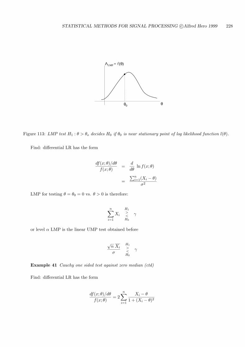
STATISTICAL METHODS FOR SIGNAL PROCESSING c©Alfred Hero 1999 228
θ0 θ
ΛLMP = (θ)
Figure 113: LMP test H1 : θ > θo decides H0 if θ0 is near stationary point of log likelihood function l(θ).
Find: differential LR has the form
df(x; θ)/dθ
f(x; θ)=
d
dθln f(x; θ)
=∑n
i=1(Xi − θ)σ2
LMP for testing θ = θ0 = 0 vs. θ > 0 is therefore:
n∑
i=1
Xi
H1
><H0
γ
or level α LMP is the linear UMP test obtained before
√n Xi
σ
H1
><H0
γ
Example 41 Cauchy one sided test against zero median (ctd)
Find: differential LR has the form
df(x; θ)/dθ
f(x; θ)= 2
n∑
i=1
Xi − θ
1 + (Xi − θ)2
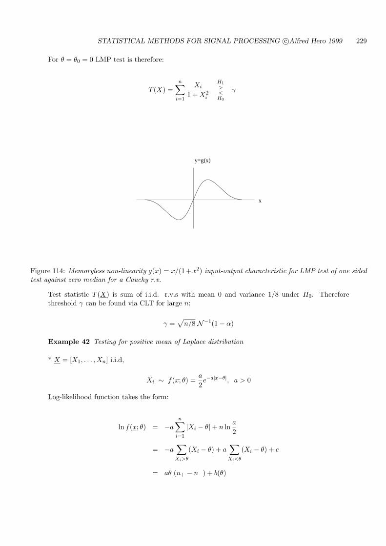
STATISTICAL METHODS FOR SIGNAL PROCESSING c©Alfred Hero 1999 229
For θ = θ0 = 0 LMP test is therefore:
T (X) =n∑
i=1
Xi
1 + X2i
H1
><H0
γ
x
y=g(x)
Figure 114: Memoryless non-linearity g(x) = x/(1+x2) input-output characteristic for LMP test of one sidedtest against zero median for a Cauchy r.v.
Test statistic T (X) is sum of i.i.d. r.v.s with mean 0 and variance 1/8 under H0. Thereforethreshold γ can be found via CLT for large n:
γ =√
n/8 N−1(1− α)
Example 42 Testing for positive mean of Laplace distribution
* X = [X1, . . . , Xn] i.i.d,
Xi ∼ f(x; θ) =a
2e−a|x−θ|, a > 0
Log-likelihood function takes the form:
ln f(x; θ) = −an∑
i=1
|Xi − θ|+ n lna
2
= −a∑
Xi>θ
(Xi − θ) + a∑
Xi<θ
(Xi − θ) + c
= aθ (n+ − n−) + b(θ)
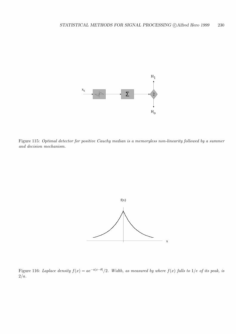
STATISTICAL METHODS FOR SIGNAL PROCESSING c©Alfred Hero 1999 230
Ho
H1
> <
xk
Σ
Figure 115: Optimal detector for positive Cauchy median is a memoryless non-linearity followed by a summerand decision mechanism.
x
f(x)
Figure 116: Laplace density f(x) = ae−a|x−θ|/2. Width, as measured by where f(x) falls to 1/e of its peak, is2/a.
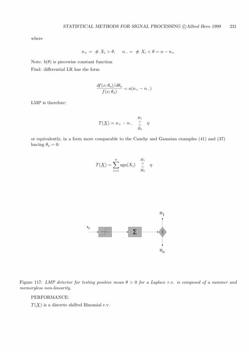
STATISTICAL METHODS FOR SIGNAL PROCESSING c©Alfred Hero 1999 231
where
n+ = # Xi > θ, n− = # Xi < θ = n− n+
Note: b(θ) is piecewise constant function
Find: differential LR has the form
df(x; θo)/dθo
f(x; θo)= a(n+ − n−)
LMP is therefore:
T (X) = n+ − n−H1
><H0
η
or equivalently, in a form more comparable to the Cauchy and Gaussian examples (41) and (37)having θo = 0:
T (X) =n∑
i=1
sgn(Xi)H1
><H0
η
Ho
H1
> <
xk
Σ
Figure 117: LMP detector for testing positive mean θ > 0 for a Laplace r.v. is composed of a summer andmemoryless non-linearity.
PERFORMANCE:
T (X) is a discrete shifted Binomial r.v.
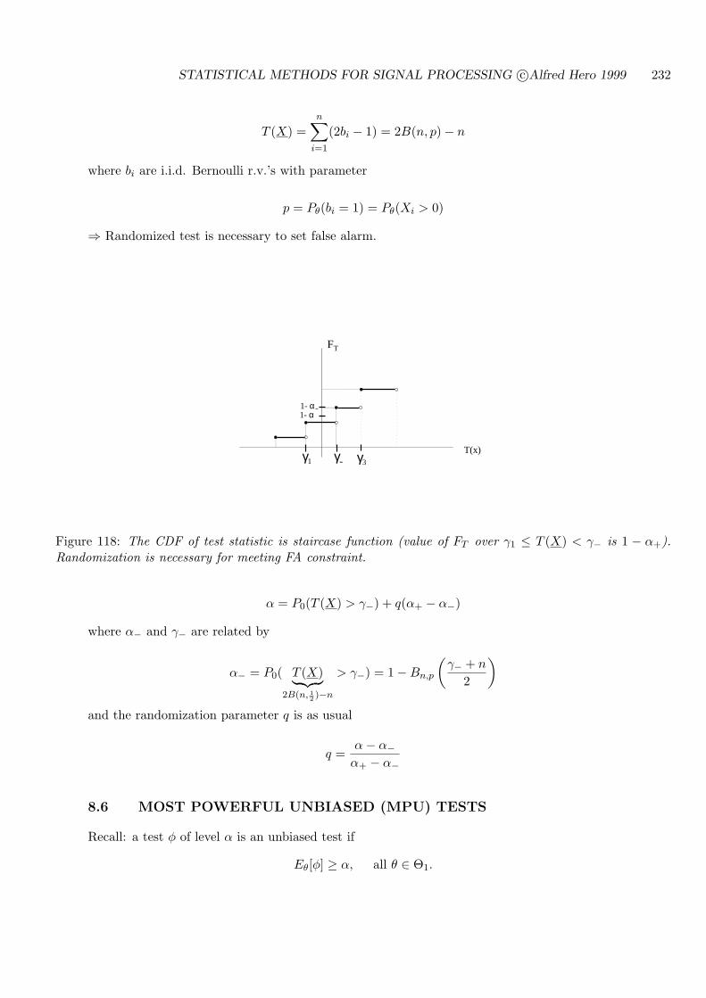
STATISTICAL METHODS FOR SIGNAL PROCESSING c©Alfred Hero 1999 232
T (X) =n∑
i=1
(2bi − 1) = 2B(n, p)− n
where bi are i.i.d. Bernoulli r.v.’s with parameter
p = Pθ(bi = 1) = Pθ(Xi > 0)
⇒ Randomized test is necessary to set false alarm.
T(x)
FT
γ1 γ- γ3
1- α1- α−
Figure 118: The CDF of test statistic is staircase function (value of FT over γ1 ≤ T (X) < γ− is 1 − α+).Randomization is necessary for meeting FA constraint.
α = P0(T (X) > γ−) + q(α+ − α−)
where α− and γ− are related by
α− = P0( T (X)︸ ︷︷ ︸2B(n, 12 )−n
> γ−) = 1−Bn,p
(γ− + n
2
)
and the randomization parameter q is as usual
q =α− α−α+ − α−
8.6 MOST POWERFUL UNBIASED (MPU) TESTS
Recall: a test φ of level α is an unbiased test if
Eθ[φ] ≥ α, all θ ∈ Θ1.
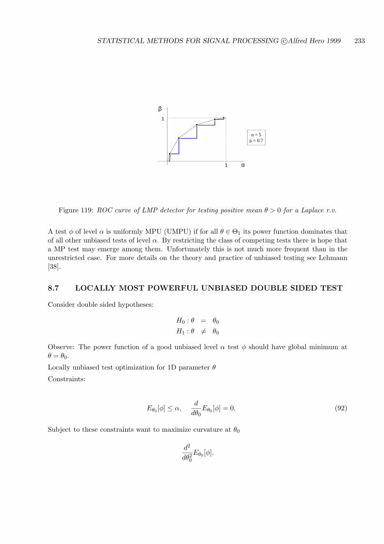
STATISTICAL METHODS FOR SIGNAL PROCESSING c©Alfred Hero 1999 233
1
1
α
β
n = 5p = 0.7
Figure 119: ROC curve of LMP detector for testing positive mean θ > 0 for a Laplace r.v.
A test φ of level α is uniformly MPU (UMPU) if for all θ ∈ Θ1 its power function dominates thatof all other unbiased tests of level α. By restricting the class of competing tests there is hope thata MP test may emerge among them. Unfortunately this is not much more frequent than in theunrestricted case. For more details on the theory and practice of unbiased testing see Lehmann[38].
8.7 LOCALLY MOST POWERFUL UNBIASED DOUBLE SIDED TEST
Consider double sided hypotheses:
H0 : θ = θ0
H1 : θ 6= θ0
Observe: The power function of a good unbiased level α test φ should have global minimum atθ = θ0.
Locally unbiased test optimization for 1D parameter θ
Constraints:
Eθ0 [φ] ≤ α,d
dθ0Eθ0 [φ] = 0. (92)
Subject to these constraints want to maximize curvature at θ0
d2
dθ20
Eθ0 [φ].

STATISTICAL METHODS FOR SIGNAL PROCESSING c©Alfred Hero 1999 234
β(θ)
β∗(θ)
θ
α
Figure 120: Power curve of most powerful unbiased test (MPU) dominates that of all other unbiased tests ofthe same FA level.
αd
PD
Figure 121: Power curve of a good locally unbiased test has minimum at α with maximum curvature.

STATISTICAL METHODS FOR SIGNAL PROCESSING c©Alfred Hero 1999 235
Using Lagrange multipliers it is easily shown that the test function φ which solves this constrainedmaximization problem has the form:
φ(x) =
1, d2f(x; θ0)/dθ20 > η(f(x; θ0) + ρ df(x; θ0)/dθ0)
q d2f(x; θ0)/dθ20 = η(f(x; θ0) + ρ df(x; θ0)/dθ0)
0 d2f(x; θ0)/dθ20 < η(f(x; θ0) + ρ df(x; θ0)/dθ0)
(93)
where ρ, η, q are selected to satisfy the two constraints.
In some cases, one can meet the constraints by selecting ρ = 0 and varying only q ∈ [0, 1] andη ∈ [0,∞). In this situation, the locally optimal test (93) reduces to the simpler (randomized)LRT form
d2f(x; θ0)/dθ20
f(x; θ0)
H1
><H0
η.
Example 43 Double sided test against zero mean of Gaussian sample with known variance
Step 1: Find derivatives of p.d.f. of sufficient statistic X (Here for clarity we define its pdf asfX(v; µ) for v ∈ IR).
fX(v; µ) =1√
2πσ2/ne− (v−µ)2
2σ2/n
dfX(v; µ)/dµ =(n/σ2
)(v − µ)fX(v;µ)
d2fX(v;µ)dµ2 =(n/σ2
)[n/σ2(v − µ)2 − 1]fX(v; µ)
Thus LMPU LRT is
X2 − σ2/n
σ2/n + ρX
H1
><H0
η
Step 2: Select ρ, η to satisfy constraints
First we attempt to satisfy constraints with ρ = 0 and η a free variable.
For this case LMPU LRT reduces to
|X|H1
><H0
γ (94)
Since
X ∼ N (0, σ2/n), under H0
we have
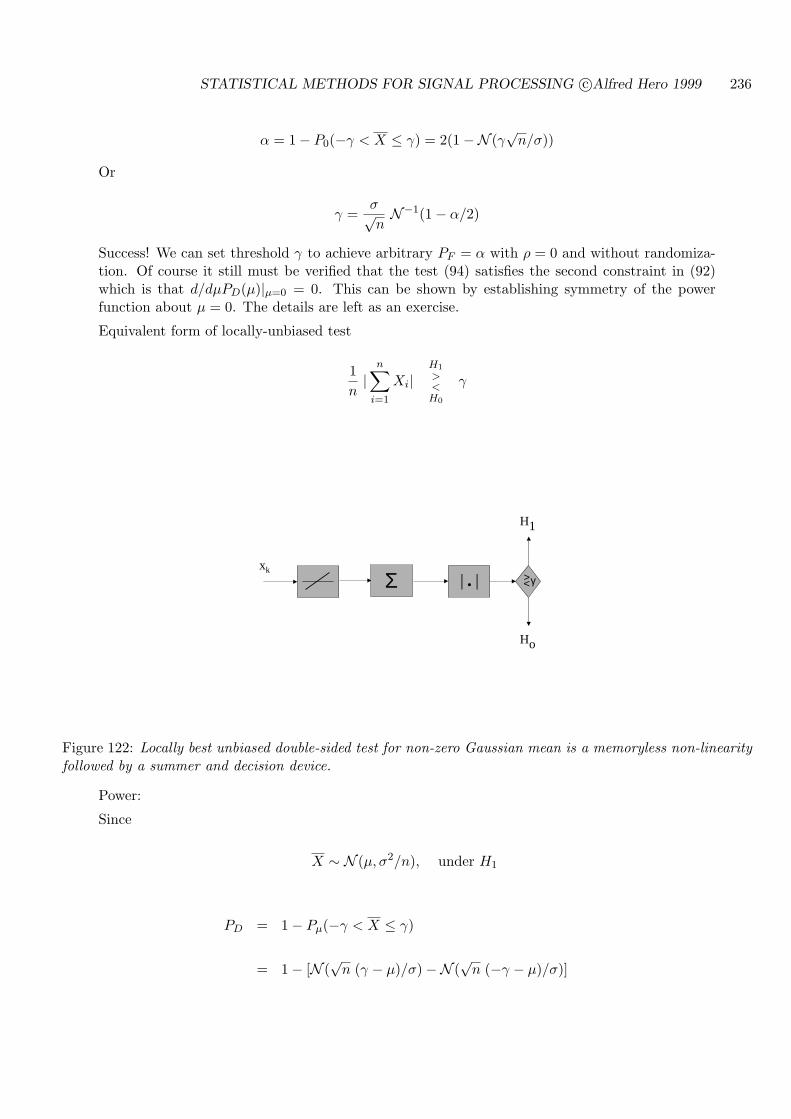
STATISTICAL METHODS FOR SIGNAL PROCESSING c©Alfred Hero 1999 236
α = 1− P0(−γ < X ≤ γ) = 2(1−N (γ√
n/σ))
Or
γ =σ√nN−1(1− α/2)
Success! We can set threshold γ to achieve arbitrary PF = α with ρ = 0 and without randomiza-tion. Of course it still must be verified that the test (94) satisfies the second constraint in (92)which is that d/dµPD(µ)|µ=0 = 0. This can be shown by establishing symmetry of the powerfunction about µ = 0. The details are left as an exercise.
Equivalent form of locally-unbiased test
1n|
n∑
i=1
Xi|H1
><H0
γ
Ho
H1
> <
xkγΣ | . |
Figure 122: Locally best unbiased double-sided test for non-zero Gaussian mean is a memoryless non-linearityfollowed by a summer and decision device.
Power:
Since
X ∼ N (µ, σ2/n), under H1
PD = 1− Pµ(−γ < X ≤ γ)
= 1− [N (√
n (γ − µ)/σ)−N (√
n (−γ − µ)/σ)]

STATISTICAL METHODS FOR SIGNAL PROCESSING c©Alfred Hero 1999 237
= 1−N (N−1(1− α/2)− d)−N (N−1(1− α/2) + d)
where as usual:
* d =√
n µ/σ is detectability index
βUMP (µ > 0)βUMP (µ < 0)
βLMP
d
PD
Figure 123: Power curve of LMPU test for for non-zero Gaussian mean with known variance as a functionof values of d.
Remark:
* It can be shown that in the Gaussian example above the LMPU test is actually UMPU. SeeFerguson [16].
The LMPU strategy can in principle be extended to multiple parameters as follows. Assume
θ = [θ1, . . . , θp]T
and let’s test the hypotheses:
H0 : θ = θ0
H1 : θ 6= θ0
Constraints:
Eθ0[φ] ≤ α, ∇θ0
Eθ0[φ] = 0) (95)
Maximize:
trace∇2
θ0Eθ0
[φ]
STATISTICAL METHODS FOR SIGNAL PROCESSING c©Alfred Hero 1999 238
where trace A denotes trace of matrix A.
This is a similar optimization as we encountered in proving the Neyman Pearson Lemma. However,now there are p+1 constraints as indicated in (95). One of them is due to the false alarm constraintand p of them are due to constraining the gradient vector to zero. The optimal test can be foundby applying Lagrange multipliers and has the form
trace∇2
θ0f(x; θ0)
f(x; θ0) +∑p
i=1 ρi∂f(x; θ0)/∂θ0i
H1
><H0
η,
where ρ1, . . . , ρp, η are selected to satisfy the constraints (possibly with randomization).
8.8 CFAR DETECTION
A sometimes reasonable condition is to require that tests have constant false alarm rate (CFAR),i.e. constant PF (θ) over θ ∈ Θ0. Then one attemps to find a UMP CFAR test. The setup is asfollows:
Constraint:Eθ[φ] = α, θ ∈ Θ0
Maximize:Eθ[φ], θ ∈ Θ1
A effective methodology for finding CFAR tests is by the use of invariance principles [33]. CFARtests are also known as similar tests and for more information see [38].
8.9 INVARIANT TESTS
Consider the general case where we have partition of θ
θ = [ϕ1, . . . , ϕp, ξ1, . . . , ξq︸ ︷︷ ︸nuisance parameters
]T
and X ∼ f(x;ϕ, ξ)
It is desired to test single sided hypotheses
H0 : ϕ = 0, ξ = ξo
H1 : ϕ > 0, ξ = ξo
where ξo∈ IRq is unknown ⇒ UMP does not usually exist.
Invariant tests seek to find a transformation (compression) of the data
Z = Z(X)
which satisfies:
Property 1. Z contains (almost) as much information concerning ϕ as X
STATISTICAL METHODS FOR SIGNAL PROCESSING c©Alfred Hero 1999 239
Property 2. Distribution of Z is not a function of ξ.
Due to Property 2, if we throw away x and retain only
Z ∼ f(z; ϕ)
then we are back to testing simpler hypotheses for which an UMP may exist
H0 : ϕ = 0H1 : ϕ > 0
The theory of optimal invariant tests is treated in detail in [33] in which invariance is referred toas exact robustness.
For now we concentrate on a particular suboptimal “invariant” approach
8.10 GENERALIZED LIKELIHOOD RATIO TEST
We now turn to one of the most prevalent methods of dealing with detection for composite hy-potheses. Unlike the previous methods, which were all motivated by solving a performance drivenoptimization problem, the generalized likelihood ratio test (GLRT) is better looked at as a heuris-tic principle than as a test strategy having assured optimality properties. However, as will bediscussed below, the GLRT is a straightforward procedure and it does have asymptotic (large n)optimality properties that are major attractions.
We consider the general composite hypotheses
H0 : θ ∈ Θ0
H1 : θ ∈ Θ1
The GLRT can be defined as an “estimate-and-plug” procedure to test H0 vs. H1:
Step 1: Find good estimates θ0 and θ1 of θ under H0 and H1
Step 2: substitute these estimates into the LR statistic
Using this procedure we obtain the GLRT
Λ =f(x; θ1)
f(x; θ0)
H1
><H0
η
where η is selected to give FA level α
Any consistent estimators will ensure that the GLRT has favorable asymptotic properties. How-ever, the most common case of the GLRT is when the estimators θ1 and θ0 are MLEs:
ΛGLR =maxθ∈Θ1 f(x; θ)maxθ∈Θ0 f(x; θ)
H1
><H0
η
Note: these MLE’s are constrained to θ ∈ Θ0 and θ ∈ Θ1, respectively.
STATISTICAL METHODS FOR SIGNAL PROCESSING c©Alfred Hero 1999 240
For a simple hypothesis H0 the GLRT reduces to
ΛGLR =supθ∈Θ1
f(x; θ)f(x; θ0)
= supθ∈Θ1
Λ(θ) = Λ(θ1).
whereΛ(θ) =
f(x; θ)f(x; θ0)
8.10.1 PROPERTIES OF GLRT
The following properties are stated simply and without proof but can be expected to hold forsmooth likelihood functions and a simple null hypothesis. For proofs of these properties the readeris referred to [39] or [7].
1. If an UMP test exists then the GLRT will be identical to it.
2. Let observations X = [X1, . . . , Xn]T be i.i.d. Then, since the MLE θ is a consistent estimator,as n →∞ the GLRT is asymptotically UMP.
3. The GLR test statistic for testing a double sided alternative hypothesis has a Chi-squarelimiting distribution under H0 as n → ∞. Specifically, assume that the unknown parameters arepartitioned as
θ = [ϕ1, . . . , ϕp, ξ1, . . . , ξq︸ ︷︷ ︸nuisance parameters
]T
and consider the GLRT for the simple null and double-sided alternative hypotheses
H0 : ϕ = ϕ0, ξ = ξ
o
H1 : ϕ 6= ϕ0, ξ = ξ
o
where ξo
is unknown. Then for large n
2 lnΛGLR(X) ∼ χp, under H0. (96)
8.11 BACKGROUND REFERENCES
Any of the references cited in the last chapter will have some discussion of the problem of testingcomposite hypotheses. Lehmann [38] has comprehensive coverage of minimax, similarity (CFAR),unbiased tests, and other methods. Invariance principles have been applied to many problems insignal processing and communications [?],[10], [9], [60]. The book by Kariya and Sinha [33] is acomprehensive, advanced level, reference on invariance principles, robustness and GLR’s (thereinreferred to as likelihood principles) relevant to these studies. Application of invariance principlescan be viewed as one way to figure out a transformation of the data that makes the resultanttransformed measurements have more tractable density functions under H0 or H1. Viewed inthis way these principles can be interpreted as a special application of the transformation method,discussed in the context of robust exploratory data analysis in the book by Hoaglin, Mosteller andTukey [27]. Another approach, that we did not discuss here, is the application of non-parametric

STATISTICAL METHODS FOR SIGNAL PROCESSING c©Alfred Hero 1999 241
techniques, also called ”distribution-free inference,” to handle unknown parameters in testing ofcomposite hypotheses. The book by Hollander and Wolfe [28] covers this topic from a generalstatistical point of view and the edited book by Kassam and Thomas [35] covers nonparametricdetection theory for applications in signal processing, communications and control.
8.12 EXERCISES
8.1 The observations xini=1 are i.i.d. exponential xi ∼ fθ(x) = βe−βx, where x, β ≥ 0. Consider
testing the following single sided hypotheses
H0 : β = β0
H1 : β > β0
(a) First find the MP test of level α for the simple alternative H1 : β = β1 where β1 >β0. Express the threshold in terms of the Gamma distribution (distribution of n i.i.d.exponential r.v.s). Next establish that your test is UMP for the single sided compositeH1 above.
(b) Specialize the results of (a) to the case of a single observation n = 1 and derive the ROCcurve. Plot your curve for β1/β0 = 1, 5, 10.
(c) Derive the locally most powerful test (LMPT) for the single sided hypotheses (maximizeslope of power subject to FA constraint) and verify that it is identical to the UMP test.
(d) Now consider testing the double sided hypotheses
H0 : β = β0
H1 : β 6= β0
Derive the LMPT (maximize curvature of power subject to FA constraint and zero slopecondition). Derive the ROC for n = 1 and compare to the ROC of part (b) over theregion β > β0.
(e) Derive the GLRT for the double sided hypotheses of part (d). Compare to your answerobtained in part (d).
8.2 Let Z be a single observation having density function
pθ(z) = (2θz + 1− θ), 0 ≤ z ≤ 1
where −1 ≤ θ ≤ 1.
(a) Is there a uniformly most powerful test between the composite hypotheses
H0 : θ = 0H1 : θ 6= 0
and, if so, what is it?(b) Find the generalized likelihood ratio test for these hypotheses.(c) Now assume that under H1 the parameter θ has prior density p(θ) = |θ|I[−1,1](θ) so that
under H1 the density of Z is f1(z) =∫
f(z|θ)pθ(θ)dθ, where f(z|θ) = pθ(z). Find theMP test between hypotheses H0 and this new H1. What if the prior density were theassymetric p(θ) = 1
2(θ + 1)I[−1,1](θ)?
STATISTICAL METHODS FOR SIGNAL PROCESSING c©Alfred Hero 1999 242
8.3 A random variable X has density
f(x; θ) =1 + θx
2, −1 ≤ x ≤ 1
where θ ∈ [−1, 1].(a) Find the MP test of level α for testing the simple hypotheses
H0 : θ = θ0
H1 : θ = θ1
based on a single sample x, where θ0 ∈ [−1, 0] and θ1 ∈ (0, 1] are known. Derive and plotthe ROC when θ0 = 0.
(b) Is there a UMP test of level α, and if so what is it, for the following hypotheses?
H0 : θ = 0H1 : θ > 0
(c) Now consider testing the doubly composite hypotheses
H0 : θ ≤ 0H1 : θ > 0
Find the GLRT for the above hypotheses. Derive the threshold of the GLRT that ensuresthe level α condition maxθ∈[−1,0] PFA(θ) ≤ α.
8.4 Available is an i.i.d. sample of a Poisson r.v. with distribution pθ(k) = Pθ(xi = k) = θk
k! e−θ,
k = 0, 1, 2, . . ..(a) Find the GLRT for testing the hypotheses
H0 : θ = θ0
H1 : θ 6= θ0
Do not attempt to set the exact threshold for level α.In the following parts of this exercise you will show how to set the GLRT threshold underthe large n Chi-square approximation to the GLRT test statistic Λ = maxθ 6=θopθ(x)/pθo(x).
(b) Directly show that under H0 the statistic 2 log Λ is asymptotically Chi-square with 1 d.f.by expanding Λ = Λ(xi) about the sample mean xi = θo, neglecting all terms of order(xi − θo)3 and higher, and recalling that (N (0, 1))2 is Chi-square with 1 d.f.
(c) Using the result of part (b) set the threshold of your GLRT in part (a).(d) Using the asymptotic results of part (b) find the GLRT between
H0 : θ ≤ θ0
H1 : θ > θ0
with threshold.8.5 Let X1, X2, . . . , Xn be i.i.d. random variables with the marginal density Xi ∼ f(x) = εg(x)+
(1− ε)h(x), where ε ∈ [0, 1] is a non-random constant and g(x) and h(x) are known densityfunctions. It is desired to test the composite hypotheses
H0 : ε = 1/2 (97)H1 : ε > 1/2 (98)
STATISTICAL METHODS FOR SIGNAL PROCESSING c©Alfred Hero 1999 243
(a) Find the most powerful (MP) test between H0 and the simple hypothesis H1 : ε = ε1,where ε1 > 1/2 (you needn’t solve for the threshold). Is your MP test a UMP test of thecomposite hypotheses (98)?
(b) Find the locally most powerful (LMP) test for (98). Show how you can use the CLT toset the threshold for large n.
(c) Find the generalized LRT (GLRT) test for (98) in the case of n = 1. Compare to youranswer in part (b).
8.6 Let Xini=1 be i.i.d. following an exponential distribution
f(x; θ) = θe−θx, x ≥ 0
with θ > 0. You are to design a test of the hypotheses
H0 : θ = θ0
H1 : θ 6= θ0
Here we explore various testing strategies.
(a) Show that the GLRT reduces to a test on the sum of the Xi’s and derive the threshold toattain FA level α (Hint: the sum of n standard (mean = 1) exponential r.v.s is standardGamma with parameter n).
(b) Now assume that H0 and H1 have equal prior probabilities p = 1/2 and that, conditionedon H1, θ itself follows an exponential distribution of the form f(θ) = βe−βθ, θ ≥ 0, whereβ > 0 is known. Find the form of the Bayes LRT (with threshold) which attains minimumprobability of decision error. What happens as β →∞?.
8.7 As in Exercise 4.24, let n i.i.d. realizations be available from the geometric mixture fGspecified by (50) and (51). Assume that φ1, φ2 are known and φ1 6= φ2.
(a) Consider the hypothesis testing problem on fG
H0 : ε = 0H1 : ε > 0.
Does a level α UMP test for these hypotheses exist? If so what is it? If not derive aGLRT test. You must specify a threshold of level α (you can assume large n).
(b) Consider the hypothesis testing problem on fG
H0 : ε = 1/2 (99)H1 : ε 6= 1/2. (100)
Does a level α UMP test for these hypotheses exist? If so what is it? If not derive aGLRT test. You must specify a threshold of level α (you can assume large n).
(c) Under the identical assumptions as in part (h) find a locally most powerful unbiased testof (100) based on n i.i.d. observations from fG and compare to the GLRT.
8.8 Let X be a random variable with density f(x; θ) = (θ +1)xθ, x ∈ [0, 1] and θ > −1. Considertesting the hypotheses
H0 : θ = 0(101)
H1 : θ = θ1
STATISTICAL METHODS FOR SIGNAL PROCESSING c©Alfred Hero 1999 244
(a) Find the most powerful (MP) test of level α for testing these hypotheses and deriveexpressions for the power function and ROC curve. Does the decision region of the MPtest of level α depend on the value of θ1?. Does there exist a UMP test of level α fortesting H0 vs. H1 : θ > 0? How about for testing H0 against H1 : θ 6= 0?
(b) Assuming priors on the hypotheses p = P (H0), 1−p = P (H1) find the optimal Bayes testof (101) under the assumption that c00 = c11 = 0 and c01 = c10 = 1 (minimal probabilityof error test). Find and plot the minimum risk (probability of error) c∗(p) as a functionof p for θ1 = 1. Using these results find the mini-max Bayes detector and its thresholdfor this value of θ.
(c) Find the locally most powerful test for testing H0 vs. H1 : θ > 0 and derive an expressionfor the ROC curve.
(d) Find the GLRT for testing H0 against H1 : θ 6= 0 and derive expressions for PF and PD
in terms of the threshold and plot the ROC curve.
8.9 In this exercise you will explore the problem of detecting an anomaly in an image solely onthe basis of filtered measurements, e.g. a blurred version of the image. This type of problemis related to “non-destructive testing” and arises in many situations that we encounter in ourdaily lives, e.g., when we pass our suitcases through a security scanner at the airport. Whenthere is no noise and no anomaly the scanner outputs an image that lies in a known subspace,the span of the columns of a known n × p matrix H, denoted colspanH. You might justthink of the columns of H as blurry images of all the possible “benign” objects that one couldpack into a suitcase. An anomaly occurs when the image has components lying outside ofthis subsapce of benign objects. Of course, there is also additive noise that complicates ourability to detect such anomalies.Now we can state the anomaly detection problem as testing the hypotheses
H0 : X = Hθ + W
(102)H1 : X = ψ + Hθ + W,
where we have defined the observed image as a vector X = [X1, . . . , Xn]T , the parametervector θ = [θ1, . . . , θp]T describes the specific linear combination of benign objects present inthe suitcase, ψ = [ψ1, . . . , ψn]T describes the anomalous component of the image, and W is aGaussian noise vector with zero mean and covariance matrix cov(W ) = σ2I. We will assumethroughout this exercise that we know the matrix H and σ2. We also assume that H is fullrank: rank(H) = p ≤ n.
(a) Assume that θ is known. For known ψ what is the most powerful (MP) test of levelα for testing H0 vs. H1? Is the test you derived in part (a) UMP for testing H0 vs.H1 : X = cψ + Hθ + W , where c > 0 is an unknown constant? Is the test UMP fortotally unknown ψ?
(b) Find an expression for and plot the ROC curve (hand drawn is fine) for the test derived in(a). What function of ψ, θ, H, and σ determines the shape of the ROC, i.e., detectibilityindex?
(c) Now assume that θ is unknown but that ψ is known. Find the GLRT of level α for testing(102) and find its ROC curve. What function of ψ, θ, H, and σ determines the shape ofthe ROC, i.e., detectibility index? What happens to the detectibility when p = n?
(d) Now assume that θ and ψ are both unknown. Find the GLRT for testing (102).
STATISTICAL METHODS FOR SIGNAL PROCESSING c©Alfred Hero 1999 245
(e) Assume that ψ is known but θ is unknown. Also assume that the anomaly vector satisfiesthe constraint ψT ψ ≤ ε, ε > 0. Using the results you derived in (c) find the leastdetectable (giving lowest power) and the most detectable (giving highest power) anomalyvectors.
8.10 Assume X is a Cauchy distributed random variable with density
f(x; θ) =1π
11 + (x− θ)2
.
You are to test the hypotheses H0 : θ = 0 vs. H1 : θ > 0 based on a single realization of X.
(a) Derive the MP test of level α for testing H0 : θ = 0 vs. H1 : θ = θ1 for a fixed valueθ1 > 0.
(b) Find the decision region X1 specifying outcomes X that will result in deciding H1.(c) Show that this decision region depends on θ1 and therefore establish that no UMP exists.
8.11 In many applications it is of interest to detect deviations of a random sample from a nominalprobability model. Such deviations are called anomalies and the general problem can beformulated as a hypothesis testing problem. One popular test uses ”minimum volume sets,”and is explored in this exercise. In the following X is a single realization of a measurementvector in IRd to be tested for anomaly.Assume that a nominal density f0(x) for X is known, e.g., learned from a lot of (non-anomalous) training samples. We assume that
∫[0,1]d f0(x)dx = 1, that is, f0 is supported
on the d-dimensional unit cube [0, 1]d. We hypothesize that an anomalous observation has adensity f1 that corresponds to a broadening of f0. Arguably, the simplest model is that f1 isthe superposition of f0 and a uniform density over [0, 1]d:
f1(x) = (1− ε)f0(x) + εU(x)
where
U(x) =
1, x ∈ [0, 1]d
0, o.w.
and ε is a mixture parameter 0 < ε ≤ 1. With this model we can define the pdf of X asf(x) = (1− ε)f0(x) + εU(x) and say that a nominal measurement corresponds to ε = 0 whilean anomaly corresponds to ε > 0.
(a) First we consider the case that the anomalous density is known, i.e., ε = ε1, ε > 0. Showthat the most powerful (MP) test of level α of the ”simple anomaly hypothesis”
H0 : ε = 0H1 : ε = ε1
is of the form ”decide H1” iff0(X) ≤ η
where η is a suitably selected threshold.(b) Show that the MP test of part (a) is a minimum-volume-set in the sense that the H0-
decision region Ω∗ = x : f0(x) ≥ η is a set having minimum volume over all sets Ωsatisfying
∫Ω f0(x)dx = 1− α. (Hint: express the volume of Ω as |Ω| = ∫
φ(x)dx, whereφ(x) is the indicator function of the set Ω).
STATISTICAL METHODS FOR SIGNAL PROCESSING c©Alfred Hero 1999 246
(c) Derive the power function of the minimum-volume-set test and show that it is propor-tional to the volume of Ω.
(d) Next we consider the case that the anomalous density is unknown. Is the minimum-volume-set test of part (b) uniformly most powerful (UMP) for the ”composite anomalyhypothesis”
H0 : ε = 0H1 : ε > 0
If it is not UMP derive the locally most powerful test (LMP) of level α.(e) Now specialize to the case of a scalar observation X, i.e., d = 1, where f0(x) is the
triangular density
f0(x) =
4x, 0 ≤ x ≤ 1/24(1− x), 1/2 < x ≤ 1
0, o.w.
Find mathematical expressions for the set Ω∗ in terms of the false alarm level α, derivethe power function (as a function of ε), and the ROC curve. Plot the power functionfor several representative values of α and plot the ROC curve for several representativevalues of ε.
End of chapter

STATISTICAL METHODS FOR SIGNAL PROCESSING c©Alfred Hero 1999 247
9 COMPOSITE HYPOTHESES IN THE UNIVARIATE GAUSSIANMODEL
In this chapter we illustrate the generalized likelihood ratio testing strategy discussed in Chapter8 to hypotheses on the mean and variance of the univariate Gaussian distribution based on i.i.dmeasurements. We will deal with the following scenarios:
* Tests on mean of a single population: σ2 known
* Tests on mean of a single population: σ2 unknown
* Tests on variance of a single population: µ known
* Tests on variance of a single population: µ unknown
* Tests on equality of means in two populations
* Tests on equality of variances in two populations
* Tests on correlation between two populations
Recall the form of the density of an i.i.d. Gaussian vector X = [X1, . . . , Xn]T with mean µ andvariance σ2.
f(x; µ, σ) =(
12πσ2
)n/2
exp
(− 1
2σ2
n∑
i=1
(xi − µ)2)
9.1 TESTS ON THE MEAN: σ2 KNOWN
Case I: H0 : µ = µo, H1 : µ > µo
Case II: H0 : µ ≤ µo, H1 : µ > µo
Case III: H0 : µ = µo, H1 : µ 6= µo
We have already established that UMP test exists for Case I. You can show that same test is UMPfor case II by checking the monotone likelihood condition [38] discussed in Sec. 8.2.
9.1.1 CASE III: H0 : µ = µo, H1 : µ 6= µo
X = [X1, . . . , Xn]T i.i.d., Xi ∼ N (µ, σ2)
Here θ = µ, Θ = IR and we want to test the double sided hypothesis that the mean equals a knownparameter µ0
H0 : µ = µo
H1 : µ 6= µo.
The GLRT is of the form:
ΛGLR = maxµ6=µo
Λ(µ) =maxµ6=µo exp
(− 12σ2
∑ni=1(Xi − µ)2
)
exp(− 1
2σ2
∑ni=1(Xi − µo)2
)
We must consider two cases
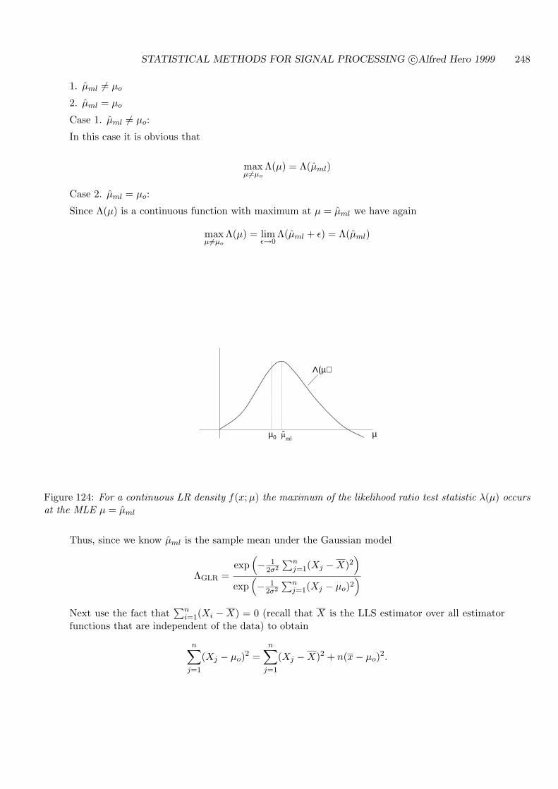
STATISTICAL METHODS FOR SIGNAL PROCESSING c©Alfred Hero 1999 248
1. µml 6= µo
2. µml = µo
Case 1. µml 6= µo:
In this case it is obvious that
maxµ6=µo
Λ(µ) = Λ(µml)
Case 2. µml = µo:
Since Λ(µ) is a continuous function with maximum at µ = µml we have again
maxµ 6=µo
Λ(µ) = limε→0
Λ(µml + ε) = Λ(µml)
µ
Λ(µ)
µ0 ml
Figure 124: For a continuous LR density f(x; µ) the maximum of the likelihood ratio test statistic λ(µ) occursat the MLE µ = µml
Thus, since we know µml is the sample mean under the Gaussian model
ΛGLR =exp
(− 1
2σ2
∑nj=1(Xj −X)2
)
exp(− 1
2σ2
∑nj=1(Xj − µo)2
)
Next use the fact that∑n
i=1(Xi −X) = 0 (recall that X is the LLS estimator over all estimatorfunctions that are independent of the data) to obtain
n∑
j=1
(Xj − µo)2 =n∑
j=1
(Xj −X)2 + n(x− µo)2.
STATISTICAL METHODS FOR SIGNAL PROCESSING c©Alfred Hero 1999 249
Hence,
ΛGLR = exp( n
2σ2(X − µo)2
)
and the GLRT is simply√
n∣∣X − µo
∣∣σ
H1
><H0
γ = N−1(1− α/2), (103)
which is identical to the LMPU (UMPU) test derived in Sec. 8.6!
Note: as predicted by our results on the asymptotic distribution of GLRTs of double sided hy-potheses (Sec. 8.10.1)
2 lnΛGLR = 2 ln
exp( n
2σ2(X − µo)2
)
=
X − µo
σ/√
n︸ ︷︷ ︸N (0,1)
2
which is distributed as a central Chi-square with 1 d.f.
A general lesson learned for GLRT’s:
⇒ for testing double sided hypotheses of form
H0 : θ = θo
H1 : θ 6= θo
if LR Λ(θ) is a continous function of θ then
maxθ 6=θo
Λ(θ) = maxθ
Λ(θ) = Λ(θml)
9.2 TESTS ON THE MEAN: σ2 UNKNOWN
Case I: H0 : µ = µo, σ2 > 0, H1 : µ > µo, σ2 > 0
Case II: H0 : µ ≤ µo, σ2 > 0, H1 : µ > µo, σ2 > 0
Case III: H0 : µ = µo, σ2 > 0, H1 : µ 6= µo, σ2 > 0
9.2.1 CASE I: H0 : µ = µo, σ2 > 0, H1 : µ > µo, σ2 > 0
From properties of the MLE for Gaussian mean and variance parameters we can easily show thatfor a realization x of X
ΛGLR =maxµ>µo,σ2>0 f(x;µ, σ2)
maxσ2>0 f(x; µo, σ2)
=
f(x; x, (xi−x)2)
f(x; µo, (xi−µo)2), x > µo
1, x ≤ µo
STATISTICAL METHODS FOR SIGNAL PROCESSING c©Alfred Hero 1999 250
where f(x;µ, σ2) is the N (µ, σ2) density and (as usual)
x = n−1n∑
i=1
xi
(xi − t)2 = n−1n∑
i=1
(xi − t)2 = σ2t .
Next observe that
f(x; x, (xi − x)2)
f(x; µo, (xi − µo)2)=
((xi − µo)2
(xi − x)2
)n/2
=
(1 +
(x− µo)2
(xi − x)2
)n/2
=(1 + T 2(x)
)n/2,
where
T (x) =x− µo√(xi − x)2
Since T 2(x) is monotone in T (x) for x > µo the GLRT based on X is
T (X) =X − µo√(Xi −X)2
H1
><H0
γ
whichisequivalenttotheonesidedt− test :√
n (X − µo)s
H1
><H0
γ′
where recall that s2 is the unbiased variance estimate for unknown mean
s2 = (n− 1)−1n∑
i=1
(Xi −X)2
PERFORMANCE:
Under H0 we have
T (X) =
N (0,1)·σ︷ ︸︸ ︷√n (Xi − µo)√√√√√√
n∑
i=1
(Xi −Xi)2
︸ ︷︷ ︸χn−1·σ2
/(n− 1)
=N (0, 1)√
χn−1/(n− 1)= Tn−1
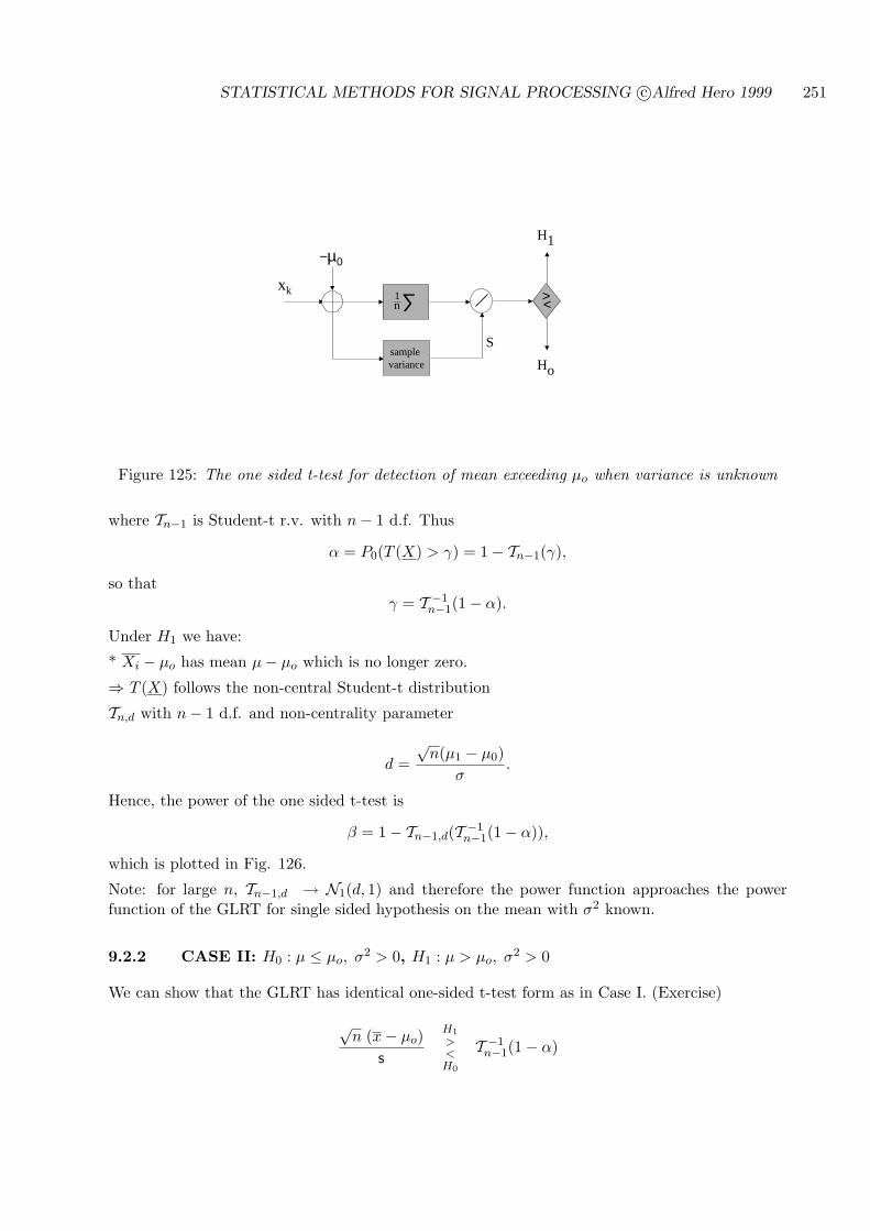
STATISTICAL METHODS FOR SIGNAL PROCESSING c©Alfred Hero 1999 251
Ho
H1
> < xk
−µ0
∑n1
sample variance
S
Figure 125: The one sided t-test for detection of mean exceeding µo when variance is unknown
where Tn−1 is Student-t r.v. with n− 1 d.f. Thus
α = P0(T (X) > γ) = 1− Tn−1(γ),
so thatγ = T −1
n−1(1− α).
Under H1 we have:
* Xi − µo has mean µ− µo which is no longer zero.
⇒ T (X) follows the non-central Student-t distribution
Tn,d with n− 1 d.f. and non-centrality parameter
d =√
n(µ1 − µ0)σ
.
Hence, the power of the one sided t-test is
β = 1− Tn−1,d(T −1n−1(1− α)),
which is plotted in Fig. 126.
Note: for large n, Tn−1,d → N1(d, 1) and therefore the power function approaches the powerfunction of the GLRT for single sided hypothesis on the mean with σ2 known.
9.2.2 CASE II: H0 : µ ≤ µo, σ2 > 0, H1 : µ > µo, σ2 > 0
We can show that the GLRT has identical one-sided t-test form as in Case I. (Exercise)
√n (x− µo)
s
H1
><H0
T −1n−1(1− α)

STATISTICAL METHODS FOR SIGNAL PROCESSING c©Alfred Hero 1999 252
α = 0.1
d
βMP (σ known)
βGLRT (σ unknown)
β
1
n = 8
0 2
Figure 126: Power curve for one sided t-test
9.2.3 CASE III: H0 : µ = µo, σ2 > 0, H1 : µ 6= µo, σ2 > 0
This case is very similar to the double sided GLRT on the mean for known σ2. We obtain GLRTas double sided t-test
√n|x− µo|
s
H1
><H0
T −1n−1(1− α/2)
with power curve
β = 1− Tn−1,d(T −1n−1(1− α/2)) + Tn−1,−d(T −1
n−1(1− α/2)).
For large n this converges to the power curve derived in the case of known variance.
9.3 TESTS ON VARIANCE: KNOWN MEAN
CASE I: H0 : σ2 = σ2o , H1 : σ2 > σ2
o
CASE II: H0 : σ2 ≤ σ2o , H1 : σ2 > σ2
o
CASE III: H0 : σ2 = σ2o , H1 : σ2 6= σ2
o
9.3.1 CASE I: H0 : σ2 = σ2o , H1 : σ2 > σ2
o
Similarly to the derivation of the GLRT for the case of one sided tests of the mean (103), thecontinuity of the Gaussian p.d.f. f(x; µ, σ2) as a function of σ2 gives:
ΛGLR =maxσ2>σ2
of(x; µ, σ2)
f(x;µ, σ2o)
=
f(x;µ, σ2
µ)
f(x; µ,σ2o)
, σ2µ > σ2
o
1, σ2µ ≤ σ2
o
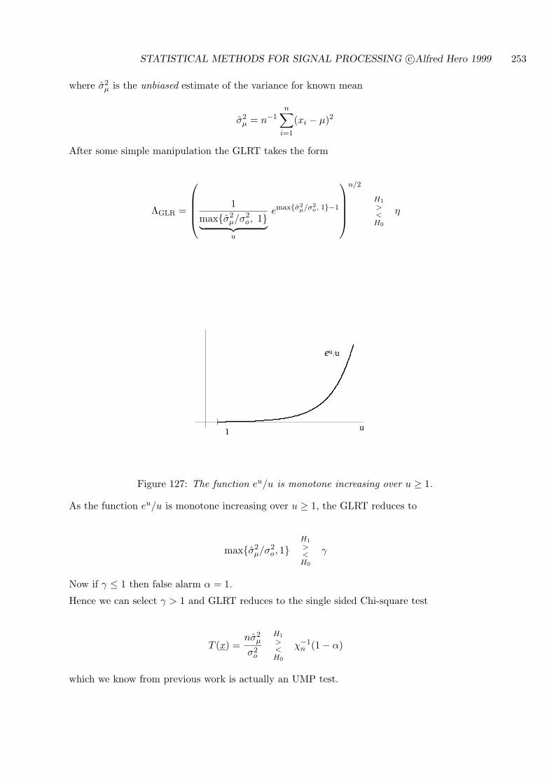
STATISTICAL METHODS FOR SIGNAL PROCESSING c©Alfred Hero 1999 253
where σ2µ is the unbiased estimate of the variance for known mean
σ2µ = n−1
n∑
i=1
(xi − µ)2
After some simple manipulation the GLRT takes the form
ΛGLR =
1maxσ2
µ/σ2o , 1︸ ︷︷ ︸
u
emaxσ2µ/σ2
o , 1−1
n/2
H1
><H0
η
u1
uue
Figure 127: The function eu/u is monotone increasing over u ≥ 1.
As the function eu/u is monotone increasing over u ≥ 1, the GLRT reduces to
maxσ2µ/σ2
o , 1H1
><H0
γ
Now if γ ≤ 1 then false alarm α = 1.
Hence we can select γ > 1 and GLRT reduces to the single sided Chi-square test
T (x) =nσ2
µ
σ2o
H1
><H0
χ−1n (1− α)
which we know from previous work is actually an UMP test.
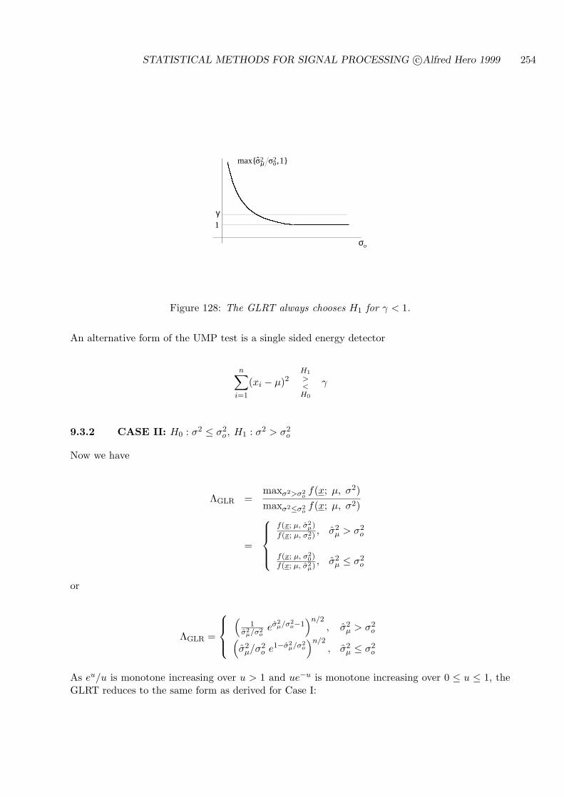
STATISTICAL METHODS FOR SIGNAL PROCESSING c©Alfred Hero 1999 254
1
γ
1 ,11max 22oµ
σo
Figure 128: The GLRT always chooses H1 for γ < 1.
An alternative form of the UMP test is a single sided energy detector
n∑
i=1
(xi − µ)2H1
><H0
γ
9.3.2 CASE II: H0 : σ2 ≤ σ2o , H1 : σ2 > σ2
o
Now we have
ΛGLR =maxσ2>σ2
of(x; µ, σ2)
maxσ2≤σ2of(x; µ, σ2)
=
f(x; µ, σ2µ)
f(x; µ, σ2o)
, σ2µ > σ2
o
f(x; µ, σ20)
f(x; µ, σ2µ)
, σ2µ ≤ σ2
o
or
ΛGLR =
(1
σ2µ/σ2
oeσ2
µ/σ2o−1
)n/2, σ2
µ > σ2o(
σ2µ/σ2
o e1−σ2µ/σ2
o
)n/2, σ2
µ ≤ σ2o
As eu/u is monotone increasing over u > 1 and ue−u is monotone increasing over 0 ≤ u ≤ 1, theGLRT reduces to the same form as derived for Case I:

STATISTICAL METHODS FOR SIGNAL PROCESSING c©Alfred Hero 1999 255
Ho
H1
> <
xkΣ
−µ
( )2+
Figure 129: GLRT for one sided test of positive shift in variance is an energy detector.
u10
uue−
Figure 130: The function ue−u is monotone increasing over 0 ≤ u ≤ 1.
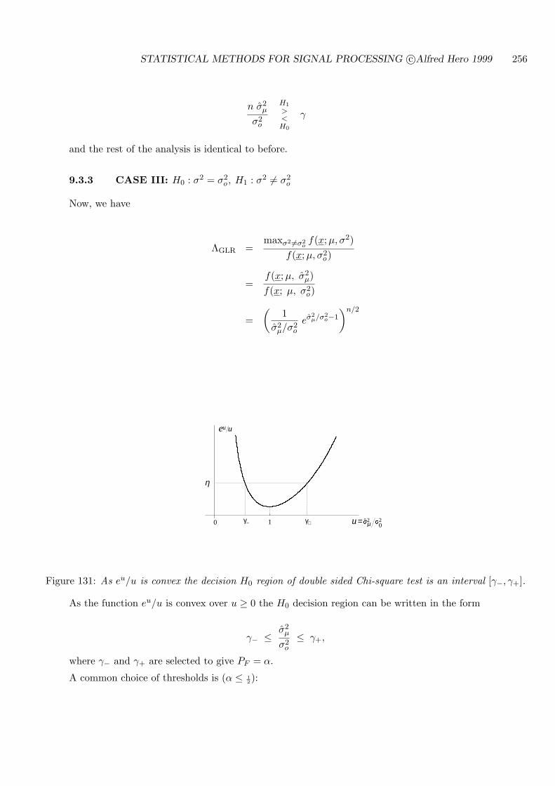
STATISTICAL METHODS FOR SIGNAL PROCESSING c©Alfred Hero 1999 256
n σ2µ
σ2o
H1
><H0
γ
and the rest of the analysis is identical to before.
9.3.3 CASE III: H0 : σ2 = σ2o , H1 : σ2 6= σ2
o
Now, we have
ΛGLR =maxσ2 6=σ2
of(x;µ, σ2)
f(x; µ, σ2o)
=f(x; µ, σ2
µ)f(x; µ, σ2
o)
=(
1σ2
µ/σ2o
eσ2µ/σ2
o−1
)n/2
1
uue
0 220
11µ=uγ− γ+
η
Figure 131: As eu/u is convex the decision H0 region of double sided Chi-square test is an interval [γ−, γ+].
As the function eu/u is convex over u ≥ 0 the H0 decision region can be written in the form
γ− ≤ σ2µ
σ2o
≤ γ+,
where γ− and γ+ are selected to give PF = α.
A common choice of thresholds is (α ≤ 12):
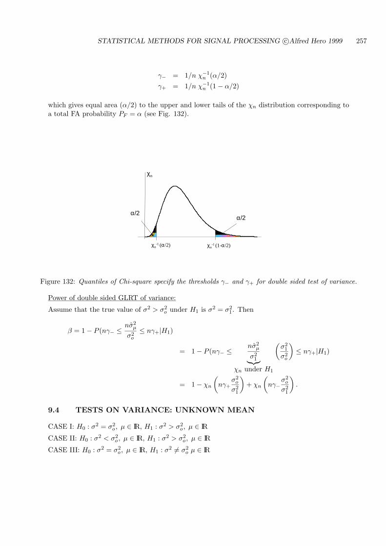
STATISTICAL METHODS FOR SIGNAL PROCESSING c©Alfred Hero 1999 257
γ− = 1/n χ−1n (α/2)
γ+ = 1/n χ−1n (1− α/2)
which gives equal area (α/2) to the upper and lower tails of the χn distribution corresponding toa total FA probability PF = α (see Fig. 132).
χn
χn-1 (α/2) χn
-1 (1-α/2)
α/2 α/2
Figure 132: Quantiles of Chi-square specify the thresholds γ− and γ+ for double sided test of variance.
Power of double sided GLRT of variance:
Assume that the true value of σ2 > σ2o under H1 is σ2 = σ2
1. Then
β = 1− P (nγ− ≤nσ2
µ
σ2o
≤ nγ+|H1)
= 1− P (nγ− ≤nσ2
µ
σ21︸︷︷︸
χn under H1
(σ2
1
σ2o
)≤ nγ+|H1)
= 1− χn
(nγ+
σ2o
σ21
)+ χn
(nγ−
σ2o
σ21
).
9.4 TESTS ON VARIANCE: UNKNOWN MEAN
CASE I: H0 : σ2 = σ2o , µ ∈ IR, H1 : σ2 > σ2
o , µ ∈ IR
CASE II: H0 : σ2 < σ2o , µ ∈ IR, H1 : σ2 > σ2
o , µ ∈ IR
CASE III: H0 : σ2 = σ2o , µ ∈ IR, H1 : σ2 6= σ2
o µ ∈ IR
STATISTICAL METHODS FOR SIGNAL PROCESSING c©Alfred Hero 1999 258
9.4.1 CASE I: H0 : σ2 = σ2o , H1 : σ2 > σ2
o
We now have
ΛGLR =maxσ2>σ2
o , µ f(x; µ, σ2)maxµ f(x;µ, σ2
o)
=
f(x; x, σ2)f(x; x,σ2
o), σ2 > σ2
o
1, σ2 ≤ σ2o
where now
σ2 = n−1n∑
i=1
(xi − x)2
This is identical to the case of known µ with µ replaced by x.
Hence, referring to work done for that case, we immediately obtain the single sided GLRT
T (x) =nσ2
σ2o
=(n− 1)s2
σ2o
H1
><H0
γ
PERFORMANCE
Under H0,
* T (X) is a Chi-square r.v. with n− 1 d.f. and thus
γ = χ−1n−1(1− α)
Under H1,
* T (X) is Chi-square with n− 1 d.f. (scaled by σ2/σo) so
β = 1− χ−1n−1(γ σ2
o/σ2)
= 1− χn−1(χ−1n−1(1− α) σ2
o/σ2)
9.4.2 CASE II: H0 : σ2 < σ2o , µ ∈ IR, H1 : σ2 > σ2
o , µ ∈ IR
GLRT is dentical to Case I.
STATISTICAL METHODS FOR SIGNAL PROCESSING c©Alfred Hero 1999 259
9.4.3 CASE III: H0 : σ2 = σ2o , µ ∈ IR, H1 : σ2 6= σ2
o µ ∈ IR
The derivation of the GLRT is completely analogous to Case III for known mean.
The H0 decision region is identical to before except that sample variance replaces σ2µ, and the test
statistic now has only n− 1 d.f.
χn−1(α/2) ≤ (n− 1)s2
σ2o
≤ χn−1(1− α/2)
The power function is identical to previous Case III for known µ except that χn CDF is replacedby χn−1 CDF.
9.5 TESTS ON EQUALITY OF MEANS: UNKNOWN VARIANCE
Two i.i.d. independent samples
X = [X1, . . . , Xn1 ]T , Xi ∼ N (µx, σ2)
Y = [Y1, . . . , Yn2 ]T , Yi ∼ N (µy, σ
2)
Case I: H0 : µx = µy, σ2 > 0, H1 : µx 6= µy, σ2 > 0
Case II: H0 : µx ≤ µy, σ2 > 0, H1 : µx > µy, σ2 > 0
X,Y have the joint density
f(x, y; µx, µy, σx, σy) =(
12πσ2
x
)n1/2 (1
2πσ2y
)n2/2
· exp
(− 1
2σ2x
n∑
i=1
(yi − µx)2 − 12σ2
y
n∑
i=1
(yi − µy)2)
where n = n1 + n2.
9.5.1 CASE I: H0 : µx ≤ µy, σ2 > 0, H1 : µx > µy, σ2 > 0
This is the case where X and Y have identical variances but possibly different means. The GLRstatistic is given by
ΛGLR =maxµx 6=µy,σ2>0 f(x, y;µx, µy, σ
2)maxµ,σ2>0 f(x, y; µ, µ, σ2)
(104)
=maxµx,µy,σ2>0 f(x, y; µx, µy, σ
2)maxµ,σ2>0 f(x, y;µ, µ, σ2)
. (105)
This can be simplified. To do this note that the MLE for the case µx 6= µy is
µx = x = n−11
n1∑
i=1
xi
µy = x = n−12
n2∑
i=1
yi
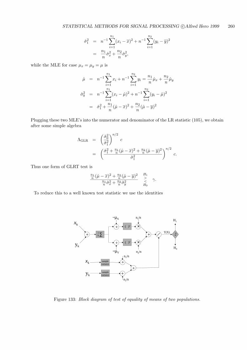
STATISTICAL METHODS FOR SIGNAL PROCESSING c©Alfred Hero 1999 260
σ21 = n−1
n1∑
i=1
(xi − x)2 + n−1n2∑
i=1
(yi − y)2
=n1
nσ2
x +n2
nσ2
y ,
while the MLE for case µx = µy = µ is
µ = n−1n1∑
i=1
xi + n−1n2∑
i=1
yi =n1
nµx +
n2
nµy
σ20 = n−1
n1∑
i=1
(xi − µ)2 + n−1n2∑
i=1
(yi − µ)2
= σ21 +
n1
n(µ− x)2 +
n2
n(µ− y)2
Plugging these two MLE’s into the numerator and denominator of the LR statistic (105), we obtainafter some simple algebra
ΛGLR =(
σ20
σ21
)n/2
c
=(
σ21 + n1
n (µ− x)2 + n2n (µ− y)2
σ21
)n/2
c.
Thus one form of GLRT test is
n1n (µ− x)2 + n2
n (µ− y)2n1n σ2
x + n2n σ2
y
H1
><H0
γ.
To reduce this to a well known test statistic we use the identities
∑n1
H0
H1
> <
xk
−µX
+
yk
+
+
( )2
( )2
×
×
+
−µY
n1/n
n2/n
T(X)
sample variance
+
n1/n
+
sample variance
+
n2/n
xk
yk
Figure 133: Block diagram of test of equality of means of two populations.

STATISTICAL METHODS FOR SIGNAL PROCESSING c©Alfred Hero 1999 261
µ− x =n1
n(y − x),
andµ− y = −n2
n(y − x),
to obtain final form of GLRT (shown in Fig. 133)
T (x, y) =
∣∣√n1n2n (y − x)
∣∣s2
H1
><H0
γ, (106)
where we have defined the pooled sample variance
s22 =1
n− 2
(n1∑
i=1
(xi − µ)2 +n2∑
i=1
(yi − µ)2)
The test (106) is the well known paired t-test.
PERFORMANCE OF PAIRED T-TEST
Under H0:Yi −Xi = N (0, σ2) ·
√(1/n1 + 1/n2),
and the test statistic is of the form of the magnitude of a Student-t random variable with n1 +n2 − 2 = n− 2 d.f:
T (X,Y ) =
∣∣∣∣∣N (0, 1)√
χn−2/n− 2
∣∣∣∣∣ .
Setting the GLRT threshold is now straightforward
α = P0(−γ < Tn−2 ≤ γ)
and we conclude that γ = T −1n−2(1− α/2). This yields the level α paired-t test
∣∣√n1n2n (y − x)
∣∣s2
H1
><H0
T −1n−2(1− α/2).
Under H1 the test statistic equivalent to the magnitude of a non-central Student-t random variablewith n− 2 d.f and non-centrality d =
√n1n2/n|µy − µx|/σ.
9.5.2 CASE II: H0 : µy ≤ µx, σ2 > 0, H1 : µy > µx, σ2 > 0
In an analogous manner to before we find that the GLRT reduces to the one sided t-test√
n1n2
n (y − x)s2
H1
><H0
γ = T −1n−2(1− α).
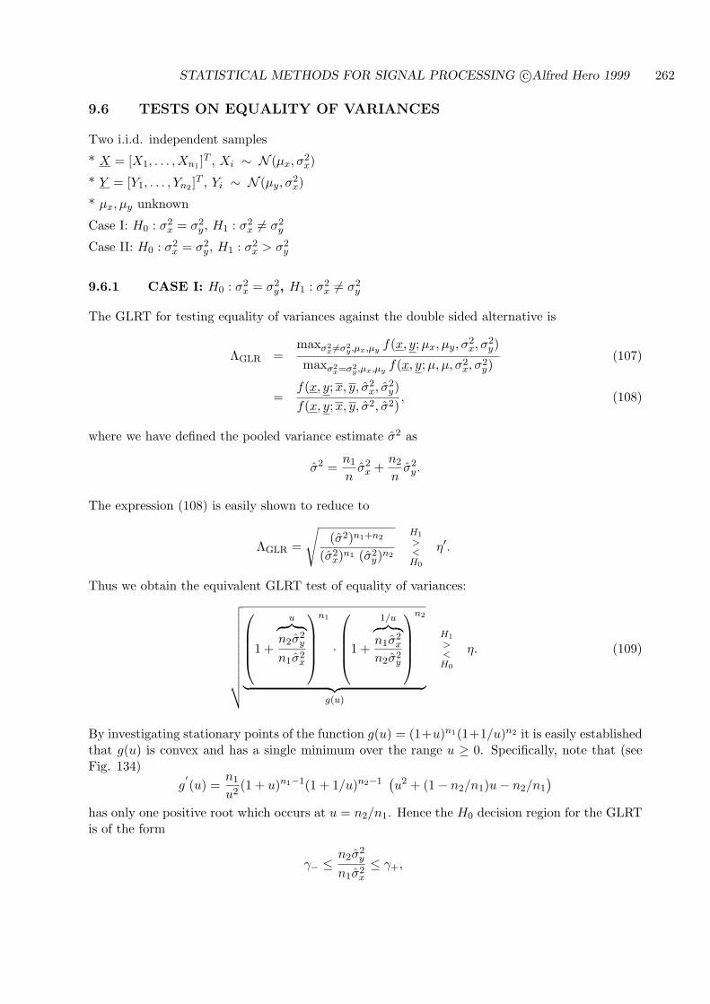
STATISTICAL METHODS FOR SIGNAL PROCESSING c©Alfred Hero 1999 262
9.6 TESTS ON EQUALITY OF VARIANCES
Two i.i.d. independent samples
* X = [X1, . . . , Xn1 ]T , Xi ∼ N (µx, σ2
x)
* Y = [Y1, . . . , Yn2 ]T , Yi ∼ N (µy, σ
2x)
* µx, µy unknown
Case I: H0 : σ2x = σ2
y , H1 : σ2x 6= σ2
y
Case II: H0 : σ2x = σ2
y , H1 : σ2x > σ2
y
9.6.1 CASE I: H0 : σ2x = σ2
y, H1 : σ2x 6= σ2
y
The GLRT for testing equality of variances against the double sided alternative is
ΛGLR =maxσ2
x 6=σ2y,µx,µy
f(x, y;µx, µy, σ2x, σ2
y)
maxσ2x=σ2
y ,µx,µyf(x, y; µ, µ, σ2
x, σ2y)
(107)
=f(x, y; x, y, σ2
x, σ2y)
f(x, y; x, y, σ2, σ2), (108)
where we have defined the pooled variance estimate σ2 as
σ2 =n1
nσ2
x +n2
nσ2
y .
The expression (108) is easily shown to reduce to
ΛGLR =
√(σ2)n1+n2
(σ2x)n1 (σ2
y)n2
H1
><H0
η′.
Thus we obtain the equivalent GLRT test of equality of variances:√√√√√√√√√√√
1 +
u︷ ︸︸ ︷n2σ
2y
n1σ2x
n1
·
1 +
1/u︷ ︸︸ ︷n1σ
2x
n2σ2y
n2
︸ ︷︷ ︸g(u)
H1
><H0
η. (109)
By investigating stationary points of the function g(u) = (1+u)n1(1+1/u)n2 it is easily establishedthat g(u) is convex and has a single minimum over the range u ≥ 0. Specifically, note that (seeFig. 134)
g′(u) =
n1
u2(1 + u)n1−1(1 + 1/u)n2−1
(u2 + (1− n2/n1)u− n2/n1
)
has only one positive root which occurs at u = n2/n1. Hence the H0 decision region for the GLRTis of the form
γ− ≤n2σ
2y
n1σ2x
≤ γ+,
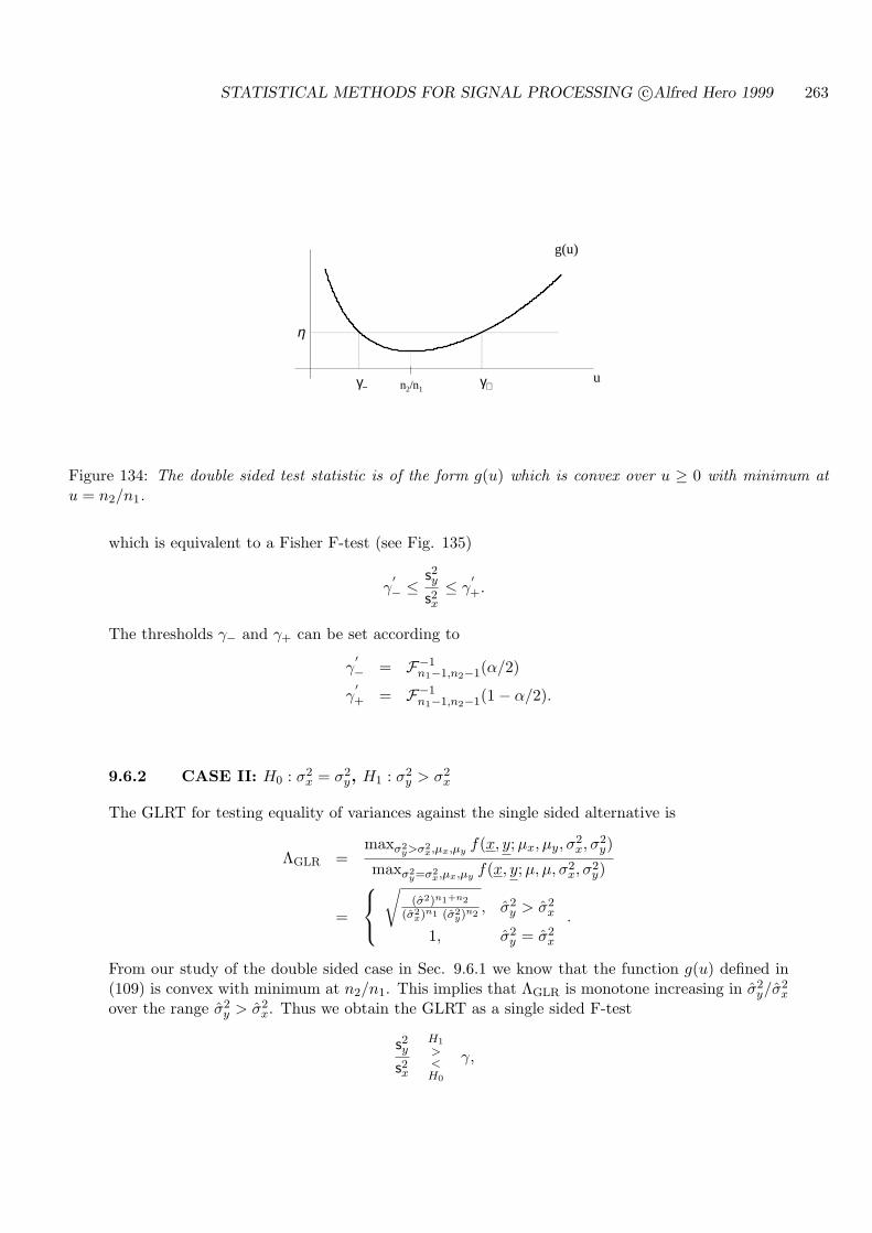
STATISTICAL METHODS FOR SIGNAL PROCESSING c©Alfred Hero 1999 263
n2/n1
η
γ− γ+u
g(u)
Figure 134: The double sided test statistic is of the form g(u) which is convex over u ≥ 0 with minimum atu = n2/n1.
which is equivalent to a Fisher F-test (see Fig. 135)
γ′− ≤
s2ys2x≤ γ
′+.
The thresholds γ− and γ+ can be set according to
γ′− = F−1
n1−1,n2−1(α/2)
γ′+ = F−1
n1−1,n2−1(1− α/2).
9.6.2 CASE II: H0 : σ2x = σ2
y, H1 : σ2y > σ2
x
The GLRT for testing equality of variances against the single sided alternative is
ΛGLR =maxσ2
y>σ2x,µx,µy
f(x, y;µx, µy, σ2x, σ2
y)
maxσ2y=σ2
x,µx,µyf(x, y; µ, µ, σ2
x, σ2y)
=
√(σ2)n1+n2
(σ2x)n1 (σ2
y)n2, σ2
y > σ2x
1, σ2y = σ2
x
.
From our study of the double sided case in Sec. 9.6.1 we know that the function g(u) defined in(109) is convex with minimum at n2/n1. This implies that ΛGLR is monotone increasing in σ2
y/σ2x
over the range σ2y > σ2
x. Thus we obtain the GLRT as a single sided F-test
s2ys2x
H1
><H0
γ,
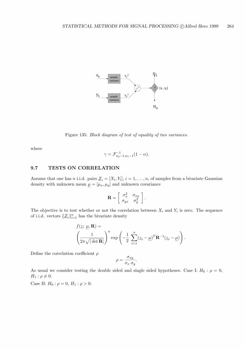
STATISTICAL METHODS FOR SIGNAL PROCESSING c©Alfred Hero 1999 264
Ho
H1xk sample variance
∈∉
yk sample variance
sx2
sy2
[γ−, γ+]
Figure 135: Block diagram of test of equality of two variances.
whereγ = F−1
n2−1,n1−1(1− α).
9.7 TESTS ON CORRELATION
Assume that one has n i.i.d. pairs Zi = [Xi, Yi], i = 1, . . . , n, of samples from a bivariate Gaussiandensity with unknown mean µ = [µx, µy] and unknown covariance
R =[
σ2x σxy
σyx σ2y
].
The objective is to test whether or not the correlation between Xi and Yi is zero. The sequenceof i.i.d. vectors Zin
i=1 has the bivariate density
f(z; µ,R) =(1
2π√| detR|
)n
exp
(−1
2
n∑
i=1
(zi − µ)TR−1(zi − µ)
).
Define the correlation coefficient ρ
ρ =σxy
σx σy.
As usual we consider testing the double sided and single sided hypotheses: Case I: H0 : ρ = 0,H1 : ρ 6= 0.
Case II: H0 : ρ = 0, H1 : ρ > 0.
STATISTICAL METHODS FOR SIGNAL PROCESSING c©Alfred Hero 1999 265
9.7.1 CASE I: H0 : ρ = ρo, H1 : ρ 6= ρo
We will show in Sec. 12.2 that the maximum of the bivariate Gaussian p.d.f. f(x, y; µx, µy,R)over µx, µy and R is equal to
maxR,µx,µy
f(x, y; µx, µy,R) =(
1(2π)2| detR|
)n/2
e−n/2
and that the maximum is attained by the joint ML estimates
µx = X
µy = Y
R =1n
n∑
i=1
[xi
yi
][xi, yi] =
[σ2
x σxy
σyx σ2y
]
where
σxy = n−1n∑
i=1
(XiYi −XY ).
Using this we can easily find GLR statistic
ΛGLR =maxR,µx,µy f(x, y; µx, µy,R)
maxdiagonal R,µx,µyf(x, y; µx, µy,R)
=
(σ2
xσ2y
σ2xσ2
y − σ2xy
)n/2
=(
11− ρ2
)n/2
,
where we have defined sample correlation coefficient
ρ =σxy
σx σy.
As ΛGLR is monotonic increasing in |ρ| we have one simple form of the GLRT
|ρ|H1
><H0
γ. (110)
An expression for the distribution under H0 of ρ(X) can be derived [56] but it is not a standardwell tabulated distribution.
A different form of the test is obtained by making a transformation on ρ
g(u) = u2/(1− u2),
which is monotone increasing in |u|. Therefore, the GLRT (110) is equivalent to
|ρ|√1− ρ2
√(n− 2)
H1
><H0
γ.
The statistic ρ/√
1− ρ2√
(n− 2) can be shown to follow the student-t distribution with n−2 d.f.[7]. Thus the level α threshold for this GLRT is
γ = T −1n−2(1− α/2).
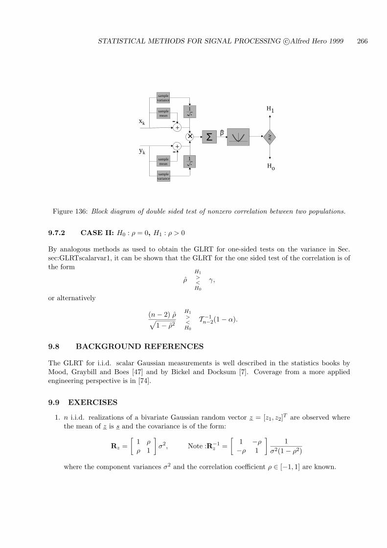
STATISTICAL METHODS FOR SIGNAL PROCESSING c©Alfred Hero 1999 266
xk
yk
+
sample mean
sample mean
+× Σ
-
-
sample variance
ρ
sample variance
•
1
•
1
Ho
H1
> <
Figure 136: Block diagram of double sided test of nonzero correlation between two populations.
9.7.2 CASE II: H0 : ρ = 0, H1 : ρ > 0
By analogous methods as used to obtain the GLRT for one-sided tests on the variance in Sec.sec:GLRTscalarvar1, it can be shown that the GLRT for the one sided test of the correlation is ofthe form
ρH1
><H0
γ,
or alternatively
(n− 2) ρ√1− ρ2
H1
><H0
T −1n−2(1− α).
9.8 BACKGROUND REFERENCES
The GLRT for i.i.d. scalar Gaussian measurements is well described in the statistics books byMood, Graybill and Boes [47] and by Bickel and Docksum [7]. Coverage from a more appliedengineering perspective is in [74].
9.9 EXERCISES
1. n i.i.d. realizations of a bivariate Gaussian random vector z = [z1, z2]T are observed wherethe mean of z is s and the covariance is of the form:
Rz =[
1 ρρ 1
]σ2, Note :R−1
z =[
1 −ρ−ρ 1
]1
σ2(1− ρ2)
where the component variances σ2 and the correlation coefficient ρ ∈ [−1, 1] are known.

STATISTICAL METHODS FOR SIGNAL PROCESSING c©Alfred Hero 1999 267
(a) Derive the MP LRT (with threshold) of the simple hypotheses
H0 : s = s0
H1 : s = s1.
For s0 = 0 is your test UMP for H1 : s 6= 0? when |ρ| > 0? How about for ρ = 0?.(b) Find the ROC of the MP LRT of part (a) and show that it is specified by the detectability
index
d2 =|E[T |H1]− E[T |H0]|2
var(T |H0)= n(s1 − s0)
TR−1z (s1 − s0)
where T is a test statistic linear in z.(c) Now assume that s0 and s1 satisfy the “power” constraints sT
0 s0 = sT1 s1 = 1. For fixed ρ
show that the optimal signal pair s1, s0 which maximizes d2 must satisfy s1− s0 = c[1, 1]when ρ < 0 while it must satisfy s1 − s0 = c[1,−1] when ρ > 0, where c is a constantensuring the power constraint.
(d) Assuming the optimal signal pair derived in part (b), for what value of ρ is the de-tectability index the worst (smallest) and for what value is it the best? Does this makesense?
2. The test on equality of a pair of means in Sec. 9.5 required equal variances and led to thepaired t-test of (106. Extend this to the case where the variances on each population may beunequal.
End of chapter

STATISTICAL METHODS FOR SIGNAL PROCESSING c©Alfred Hero 1999 268
10 STATISTICAL CONFIDENCE INTERVALS
In many cases an estimate of an unknown parameter does not suffice. one is usually also interestedin the statistical accuracy of the estimate and the estimation strategies discussed in Chapter 4do not provide any help here. Such a measure can be developed by taking a different approach:instead of seeking an estimate of the true parameter, called a point estimate, one seeks a tightinterval that covers the true parameter with specified confidence level. This approach is calledthe method of statistical confidence intervals. It turns out that confidence intervals are closelyrelated to tests of composite double sided hypotheses and we will exploit this connection in ourpresentation.
The specific topics include:
OUTLINE
* Confidence intervals via pivots
* Confidence intervals and double sided tests
* Confidence interval for mean, variance, correlation
10.1 DEFINITION OF A CONFIDENCE INTERVAL
Let θ ∈ Θ be an unknown scalar parameter and let X ∼ f(x; θ) be an observed random variable,random vector or random process. As opposed to a point estimator θ(X) which is a (random)point in the parameter space Θ, a confidence interval [T1(X), T2(X)] is a (random) interval inparameter space. Confidence intervals are also called set or interval estimators.
OBJECTIVE: find two statistics T1 = T1(X) and T2 = T2(X), T1 < T2, which specify endpointsof a random interval
[T1, T2]
that contains θ with high probability.
CONSTRUCTION OF CONFIDENCE INTERVALS
1. Fix α ∈ [0, 1]
2. For all θ ∈ Θ we require
Pθ(T1 ≤ θ ≤ T2) ≥ 1− α
The interval [T1, T2] is called a 100(1− α)% confidence interval
Equivalently:
⇒ 1− α is confidence level of statement “θ ∈ [T1, T2]”
⇒ [T1, T2] is a set estimate of θ
* Pθ(T1 ≤ θ ≤ T2) is coverage probability of the confidence interval
* 1− α is lower bound on coverage probability of a 100(1− α)% conf. interval
* T2 − T1 is the size of confidence interval
* Sometimes a level α GLRT or LMPT of double sided hypotheses can be useful for findingconfidence intervals.
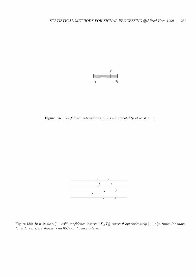
STATISTICAL METHODS FOR SIGNAL PROCESSING c©Alfred Hero 1999 269
θ
T1 T2
Figure 137: Confidence interval covers θ with probability at least 1− α.
θ
Figure 138: In n-trials a (1−α)% confidence interval [T1, T2] covers θ approximately (1−α)n times (or more)for n large. Here shown is an 85% confidence interval.

STATISTICAL METHODS FOR SIGNAL PROCESSING c©Alfred Hero 1999 270
10.2 CONFIDENCE ON MEAN: KNOWN VAR
Objective: find confidence interval on the mean µ based on i.i.d. Gaussian sample X = [X1, . . . , Xn]with known variance σ2.
APPROACH 1: Use Tchebychev inequality:
Pµ(|Xi − µ| ≥ ε) ≤
σ2/n︷ ︸︸ ︷Eµ[(Xi − µ)2]
ε2
µ area < α
∈
f(y;µ,σ)
y
Figure 139: Tchebychev inequality specifies an interval containing the mean with at least probability 1−σ2/nε2.In figure f(y; µ, σ) denotes the density of the sample mean Y = Xi.
or, setting ε = c σ/√
n
Pµ(|Xi − µ| ≥ c σ/√
n) ≤ 1c2
or equivalently
Pµ(|Xi − µ| ≤ c σ/√
n) ≥ 1− 1c2
i.e.
Pµ(Xi − c σ/√
n ≤ µ ≤ Xi + c σ/√
n) ≥ 1− 1c2
Finally take c = 1/√
α to obtain 100(1− α)% confidence interval for µ
[Xi − σ√
αn, Xi +
σ√αn
]
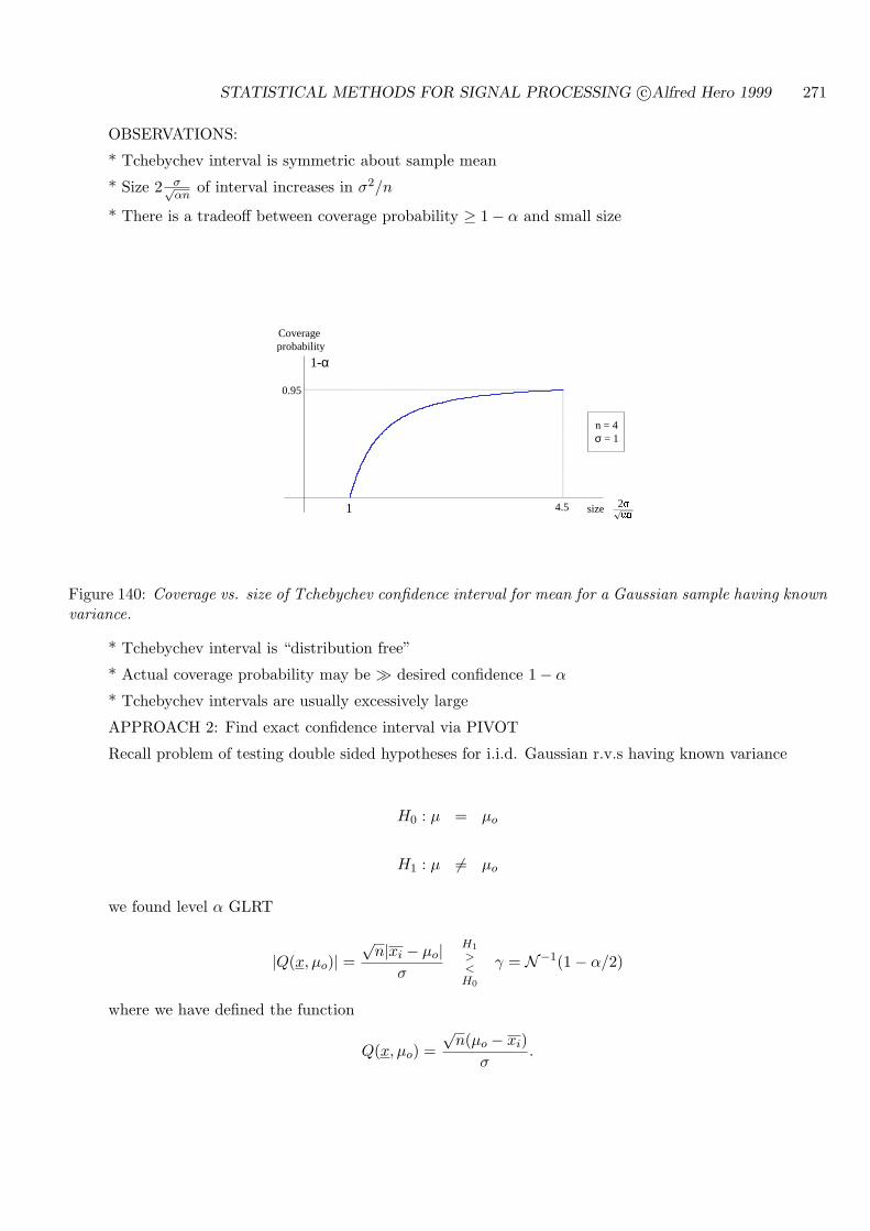
STATISTICAL METHODS FOR SIGNAL PROCESSING c©Alfred Hero 1999 271
OBSERVATIONS:
* Tchebychev interval is symmetric about sample mean
* Size 2 σ√αn
of interval increases in σ2/n
* There is a tradeoff between coverage probability ≥ 1− α and small size
Coverage probability
size1
n = 4σ = 1
1-α
.Q214.5
0.95
Figure 140: Coverage vs. size of Tchebychev confidence interval for mean for a Gaussian sample having knownvariance.
* Tchebychev interval is “distribution free”
* Actual coverage probability may be À desired confidence 1− α
* Tchebychev intervals are usually excessively large
APPROACH 2: Find exact confidence interval via PIVOT
Recall problem of testing double sided hypotheses for i.i.d. Gaussian r.v.s having known variance
H0 : µ = µo
H1 : µ 6= µo
we found level α GLRT
|Q(x, µo)| =√
n|xi − µo|σ
H1
><H0
γ = N−1(1− α/2)
where we have defined the function
Q(x, µo) =√
n(µo − xi)σ
.
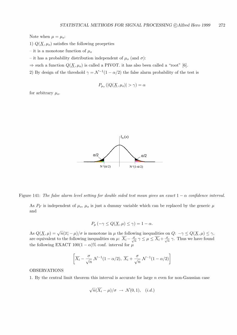
STATISTICAL METHODS FOR SIGNAL PROCESSING c©Alfred Hero 1999 272
Note when µ = µo:
1) Q(X,µo) satisfies the following proeprties
– it is a monotone function of µo
– it has a probability distribution independent of µo (and σ):
⇒ such a function Q(X,µo) is called a PIVOT. it has also been called a “root” [6].
2) By design of the threshold γ = N−1(1− α/2) the false alarm probability of the test is
Pµo (|Q(X,µo)| > γ) = α
for arbitrary µo.
α/2
fN (x)
α/2
N-1(α/2) N-1(1-α/2)
Figure 141: The false alarm level setting for double sided test mean gives an exact 1− α confidence interval.
As PF is independent of µo, µo is just a dummy variable which can be replaced by the generic µand
Pµ (−γ ≤ Q(X,µ) ≤ γ) = 1− α.
As Q(X, µ) =√
n(xi−µ)/σ is monotone in µ the following inequalities on Q: −γ ≤ Q(X,µ) ≤ γ,are equivalent to the following inequalities on µ: Xi− σ√
nγ ≤ µ ≤ Xi + σ√
nγ. Thus we have found
the following EXACT 100(1− α)% conf. interval for µ
[Xi − σ√
nN−1(1− α/2), Xi +
σ√nN−1(1− α/2)
]
OBSERVATIONS
1. By the central limit theorem this interval is accurate for large n even for non-Gaussian case
√n(Xi − µ)/σ → N (0, 1), (i.d.)
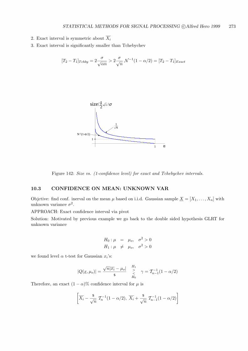
STATISTICAL METHODS FOR SIGNAL PROCESSING c©Alfred Hero 1999 273
2. Exact interval is symmetric about Xi
3. Exact interval is significantly smaller than Tchebychev
[T2 − T1]Tchby = 2σ√αn
> 2σ√nN−1(1− α/2) = [T2 − T1]Exact
N-1(1-α/2)
.1
α
σ/21 nsize⋅
1
1
Figure 142: Size vs. (1-confidence level) for exact and Tchebychev intervals.
10.3 CONFIDENCE ON MEAN: UNKNOWN VAR
Objctive: find conf. inerval on the mean µ based on i.i.d. Gaussian sample X = [X1, . . . , Xn] withunknown variance σ2.
APPROACH: Exact confidence interval via pivot
Solution: Motivated by previous example we go back to the double sided hypothesis GLRT forunknown variance
H0 : µ = µo, σ2 > 0H1 : µ 6= µo, σ2 > 0
we found level α t-test for Gaussian xi’s:
|Q(x, µo)| =√
n|xi − µo|s
H1
><H0
γ = T −1n−1(1− α/2)
Therefore, an exact (1− α)% confidence interval for µ is
[Xi − s√
nT −1
n (1− α/2), Xi +s√nT −1
n−1(1− α/2)]
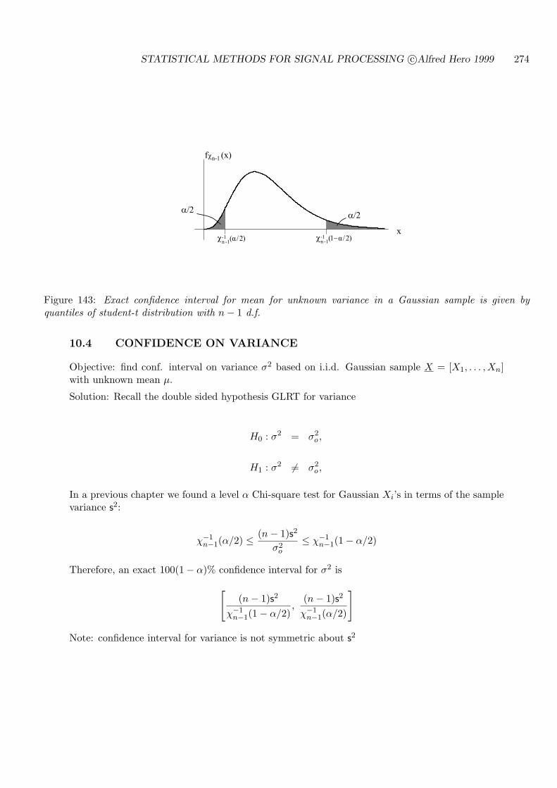
STATISTICAL METHODS FOR SIGNAL PROCESSING c©Alfred Hero 1999 274
f n-1 (x)
)2/(1-1-n
)2/1(1-1-n
x
Figure 143: Exact confidence interval for mean for unknown variance in a Gaussian sample is given byquantiles of student-t distribution with n− 1 d.f.
10.4 CONFIDENCE ON VARIANCE
Objective: find conf. interval on variance σ2 based on i.i.d. Gaussian sample X = [X1, . . . , Xn]with unknown mean µ.
Solution: Recall the double sided hypothesis GLRT for variance
H0 : σ2 = σ2o ,
H1 : σ2 6= σ2o ,
In a previous chapter we found a level α Chi-square test for Gaussian Xi’s in terms of the samplevariance s2:
χ−1n−1(α/2) ≤ (n− 1)s2
σ2o
≤ χ−1n−1(1− α/2)
Therefore, an exact 100(1− α)% confidence interval for σ2 is
[(n− 1)s2
χ−1n−1(1− α/2)
,(n− 1)s2
χ−1n−1(α/2)
]
Note: confidence interval for variance is not symmetric about s2
STATISTICAL METHODS FOR SIGNAL PROCESSING c©Alfred Hero 1999 275
10.5 CONFIDENCE ON DIFFERENCE OF TWO MEANS
Objective: find conf. interval on the difference ∆ = µx − µy of means in two i.i.d. Gaussiansamples X = [X1, . . . , Xn1 ], Y = [Y1, . . . , Yn2 ]
Solution: consider the hypotheses
H0 : ∆ = ∆o
H1 : ∆ 6= ∆o
A GLRT of level α would give a confidence interval for ∆ similiarly to before.
Recall: the t test√
n1n2n |xi − yi|
s2
H1
><H0
T −1n−2(1− α/2)
was previously derived for the double sided hypotheses
H′0 : µx = µy
H′1 : µx 6= µy
There is a difficulty, however, since ∆ does not appear any where in the test statistic. In particular
* Xi − Yi has mean ∆ under H0 : ∆ = ∆o
* therefore distribution of t-test statistic above depends on ∆ and is not a pivot
However, as Xi−Yi−∆ has mean zero under H0 and same variance as Xi−Yi, we can immediatelyidentify the following pivot
√n1n2
n (Xi − Yi −∆)s2
∼ Tn−2
Thus, the left and right endpoints of a 100(1− α)% conf. interval on ∆ are given by
Xi − Yi ∓√
n
n1n2s2 T −1
n−2(1− α/2)
10.6 CONFIDENCE ON DIFFERENCE OF TWO VARIANCES
Objective: find conf. interval on the ratio
c = σ2x/σ2
y
of variances in two i.i.d. Gaussian samples
* X = [X1, . . . , Xn1 ] , Y = [Y1, . . . , Yn2 ]
Solution: Recall that the GLRT for double sided H1 : σ2x 6= σ2
y was F-test
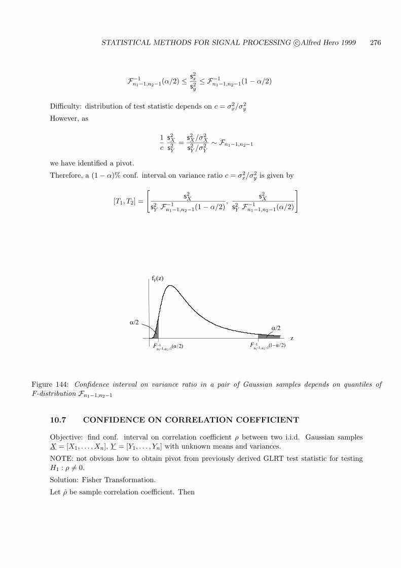
STATISTICAL METHODS FOR SIGNAL PROCESSING c©Alfred Hero 1999 276
F−1n1−1,n2−1(α/2) ≤ s2x
s2y≤ F−1
n1−1,n2−1(1− α/2)
Difficulty: distribution of test statistic depends on c = σ2x/σ2
y
However, as
1c
s2Xs2Y
=s2X/σ2
X
s2Y /σ2Y
∼ Fn1−1,n2−1
we have identified a pivot.
Therefore, a (1− α)% conf. interval on variance ratio c = σ2x/σ2
y is given by
[T1, T2] =
[s2X
s2Y F−1n1−1,n2−1(1− α/2)
,s2X
s2Y F−1n1−1,n2−1(α/2)
]
)2/1(1-1-n1,-n 21
F)2/(1-1-n1,-n 21
F
fF(z)
z
Figure 144: Confidence interval on variance ratio in a pair of Gaussian samples depends on quantiles ofF-distribution Fn1−1,n2−1
10.7 CONFIDENCE ON CORRELATION COEFFICIENT
Objective: find conf. interval on correlation coefficient ρ between two i.i.d. Gaussian samplesX = [X1, . . . , Xn], Y = [Y1, . . . , Yn] with unknown means and variances.
NOTE: not obvious how to obtain pivot from previously derived GLRT test statistic for testingH1 : ρ 6= 0.
Solution: Fisher Transformation.
Let ρ be sample correlation coefficient. Then

STATISTICAL METHODS FOR SIGNAL PROCESSING c©Alfred Hero 1999 277
υ = 12 ln
(1 + ρ
1− ρ
)= tanh−1(ρ)
has an asymptotic normal dsn with
Eθ[υ] = tanh−1(ρ)
varθ(υ) =1
n− 3
tanh-1(x)
x
Figure 145: Inverse tanh function is monotone increasing.
Hence we have a pivot
Q(X, ρ) =tanh−1(ρ)− tanh−1(ρ)
1/√
n− 3∼ N (0, 1)
This gives 100(1− α)% conf. interval on tanh−1(ρ)
[υ − 1√
n− 3N−1(1− α/2), υ +
1√n− 3
N−1(1− α/2)]
Since tanh−1(·) is monotone, the left and right endpoints T1, T2 of (1−α)% conf. interval [T1, T2]on ρ are
tanh(
υ ∓ 1√n− 3
N−1(1− α/2))
OBSERVATIONS:
1. Conf. interval is not symmetric
STATISTICAL METHODS FOR SIGNAL PROCESSING c©Alfred Hero 1999 278
2. Conf. interval prescribes a level α test of double sided hypotheses
H0 : ρ = ρo,
H1 : ρ 6= ρo
which is
φ(x) =
1, ρo 6∈ [T1, T2]
0, ρo ∈ [T1, T2]
Indeed:
E0[φ] = 1− Pρo(T1 ≤ ρo ≤ T2)
= 1− (1− α) = α
10.8 BACKGROUND REFERENCES
There are other ways to construct confidence intervals besides exploiting the double sided GLRTrelationship. As in previous chapters we refer the reader to the two excellent books by Mood,Graybill and Boes [47] and by Bickel and Docksum [7] for more general discussion of confidenceintervals. The book by Hjorth [26] covers the theory and practice of bootstrap confidence inter-vals, a powerful nonparametric but computationally intensive approach to the interval estimationproblem. A generalization of the theory of confidence intervals is the theory of confidence regions,which is briefly presented in Sec. 12.6 after we discuss the GLRT of multivariate double sidedhypotheses.
10.9 EXERCISES
10.1 Let Xini=1 be an i.i.d. sample with marginal p.d.f. f(x; θ) = θe−θx, x > 0.
(a) Show that the maximum likelihood estimator (MLE) for θ is 1X
, where X is the samplemean (you should have previously derived this in hwk 2).
(b) Show that the CR bound I−1(θ) for θ given Xini=1 is of the form: I−1(θ) = θ2
n .(c) Now, using the fact that for large n the MLE is distributed as approximatelyN (θ, I−1(θ)),
show that(
1/X1+Z(1−α
2)/√
n, 1/X
1−Z(1−α2)/√
n
)is a (1−α)·100% confidence interval for θ, where
Z(p) = N−1(p) =
x :∫ x−∞ e− 1
2x2dx/
√2π = p
is the p− th quantile of N (0, 1).
10.2 Let X = [X1, . . . ,Xn]T be a Gaussian random vector with mean µ = [µ1, . . . , µn]T andcovariance matrix RX .
(a) Show that the distribution of W def= (X− µ)T R−1X (X− µ) is Chi-Square with n degrees
of freedom (Hint: use square root factor R12X to represent (X− µ) in terms of a vector of
uncorrelated standard Gaussian variates).
STATISTICAL METHODS FOR SIGNAL PROCESSING c©Alfred Hero 1999 279
(b) Since W has a distribution which is independent of µ and RX , W is similar to a pivotfor scaler µ which can be used to generate confidence regions on µ. Assume n = 2 andlet RX be a fixed and known diagonal matrix with eigenvalues λ1 and λ2. Show that
R def= µ : (X − µ)T R−1X (X − µ) ≤ −2 lnα is a 100(1 − α)% confidence region for the
vector µ in the sense that: P (µ ∈ R) = P (W ≤ −2 lnα) = 1−α. Draw a concise pictureof this confidence region for the case µ ∈ IR2. Label and identify all quantities in yourpicture. What happens to the confidence region as λ1 → 0? Does this make sense?
10.3 This exercise establishes that a pivot always exists when the marginal CDF is strictly increas-ing. Let Xin
i=1 be an i.i.d. sample with marginal p.d.f. f(x; θ) and a CDF F (x; θ) which isstrictly increasing: F (x + ∆; θ + δ) > F (x; θ), ∆, δ > 0 .
(a) Show that the random variable F (Xi; θ) has a uniform distribution over the interval [0, 1],and that therefore − log F (Xi; θ) has an exponential distribution f(u) = e−u, u > 0.
(b) Show that the CDF of the entire sample,∏n
i=1 F (Xi; θ) is a pivot for θ. (Hint: theproduct of monotone functions is monotone).
(c) Show that a (1 − α) · 100% confidence interval for θ can be constructed since F (x; θ) ismonotone in θ using the result of part (b). (Hint: the sum of n i.i.d. exponential r.v.swith distribution f(u) = e−u, u > 0 has a Gamma density).
10.4 Use the approach of the previous problem to construct (1− α)100% confidence intervals forthe following parameters.
(a) θ is the parameter in the density f(x; θ) = 2θx + 1 − θ, 0 ≤ x ≤ 1, −1 ≤ θ ≤ 1. Verifyyour results by numerical simulation for n = 10 using Matlab. Note it may be helpful touse Matlab’s polynomial rooting procedure roots.m to find the interval endpoints. Notefor this example you cannot use double sided GLRT since the GLRT is degenerate.
(b) θ is the median of the Cauchy distribution f(xi, θ) = (1+(x−θ)2)/π. Note that numericalintegration may be required. Verify your results by numerical simulation for n = 10 usingMatlab.
10.5 Let x1, . . . , xn be an i.i.d. sample of a Poisson r.v. with distribution pθ(k) = Pθ(xi = k) =θk
k! e−θ, k = 0, 1, 2, . . .. Use the GLRT derived in Exercise 8.4 to specify a (1−α)% confidence
interval on θ.
10.6 Let Xini=1 be i.i.d. following an exponential distribution
f(x; θ) = θe−θx, x ≥ 0
with θ > 0.
(a) Derive the GLRT for the test of the hypotheses
H0 : θ = θ0
H1 : θ 6= θ0
with FA level α (Hint: the sum of n standard (mean = 1) exponential r.v.s is standardGamma with parameter n).
(b) Using the results of (a) find a (1− α)% confidence interval on θ.
End of chapter
STATISTICAL METHODS FOR SIGNAL PROCESSING c©Alfred Hero 1999 280
11 SIGNAL DETECTION IN THE MULTIVARIATE GAUSSIANMODEL
In this chapter we cover LR tests of simple hypotheses on the mean and covariance in the generalmultivariate Gaussian model. We will start with offline detection strategies when the measurementis a small dimensional vector of possibly correlated Gaussian observations. We then turn to onlinedetection for change in mean and covariance of sampled Gaussian waveforms and this will bringthe Kalman filter into the picture. This arises, for example, when we wish to decide on the mean orvariance of Gaussian random process based on its time samples, a very common problem in signalprocessing, control and communications. While the focus is on simple hypotheses some discussionof unknown parameters is given.
Specifically, we will cover the following:
1. Offline methods:
* General vector Gaussian problem
* Detection of non-random signals in noise: matched-filter
* Detection of random signals in noise: filter-squarer and estimator-correlator
2. Online methods
* On line detection of non-random signals: causal matched-filter
* On-line detection for nonstationary signals: Kalman filter detector
11.1 OFFLINE METHODS
We have the following setup.
Observation: X = [X1, . . . , Xn]T ∼ Nn(µ,R)
mean: µ = E[X] = [µ1, . . . , µn]T
covariance: R = ((cov(xi, xj)))i,j=1,...,n
R =
σ21 · · · σ1,n...
. . ....
σn,1 . . . σ2n
Joint density
f(x; µ,R) =1
(2π)n/2√|R| exp
(− 12(x− µ)TR−1(x− µ)
)
Consider simple detection problem
H0 : µ = µ0, R = R0
H1 : µ = µ1, R = R1
Likelihood ratio is
STATISTICAL METHODS FOR SIGNAL PROCESSING c©Alfred Hero 1999 281
Λ(x) =
√|R0| exp
(− 1
2(x− µ1)TR−1
1 (x− µ1))
√|R1| exp
(− 1
2(x− µ0)TR−1
0 (x− µ0))
Giving LRT
T (x) =
12(x− µ
0)TR−1
0 (x− µ0)− 1
2(x− µ1)TR−1
1 (x− µ1)
H1
><H0
γ
where
γ = log η + 12 log
|R1||R0|
Interpretation of LRT as distorted “Mahalanobis” distance test:
Define two norms in IRn
‖z‖R0 = zTR−10 z, ‖z‖R1 = zTR−1
1 z,
Norm ‖z‖R emphasizes components of z which are colinear to eigenvectors of R associated withsmall eigenvalues
Then MP-LRT takes form of a comparison between weighted distances of x to µ0
vs. µ1
‖x− µ0‖2
R0− ‖x− µ
1‖2
R1
H1
><H0
γ′
An alternative form of LRT is the quadratic test
T′(x) = 1
2xT [R−1
0 −R−11 ]x + (µT
1R−1
1 − µT0R−1
0 )xH1
><H0
γ′
γ′= log η + 1
2 log|R1||R0| + µT
1R−1
1 µ1− µT
0R−1
0 µ0
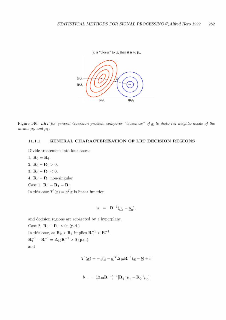
STATISTICAL METHODS FOR SIGNAL PROCESSING c©Alfred Hero 1999 282
x(µ0)2
(µ1)2
(µ0)1 (µ1)1
x is “closer” to µ1 than it is to µ0
.
Figure 146: LRT for general Gaussian problem compares “closeness” of x to distorted neighborhoods of themeans µ0 and µ1.
11.1.1 GENERAL CHARACTERIZATION OF LRT DECISION REGIONS
Divide treatement into four cases:
1. R0 = R1,
2. R0 −R1 > 0,
3. R0 −R1 < 0,
4. R0 −R1 non-singular
Case 1. R0 = R1 = R:
In this case T′(x) = aT x is linear function
a = R−1(µ1− µ
0),
and decision regions are separated by a hyperplane.
Case 2. R0 −R1 > 0: (p.d.)
In this case, as R0 > R1 implies R−10 < R−1
1 ,
R−11 −R−1
0 = ∆10R−1 > 0 (p.d.):
and
T′(x) = − 1
2(x− b)T ∆10R−1(x− b) + c
b = (∆10R−1)−1[R−11 µ
1−R−1
0 µ0]
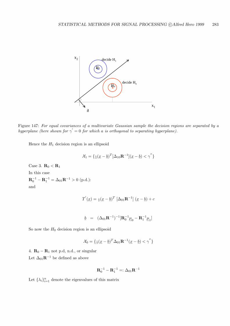
STATISTICAL METHODS FOR SIGNAL PROCESSING c©Alfred Hero 1999 283
a
µo
µ1
decide H1
decide Ho
x1
x2
Figure 147: For equal covariances of a multivariate Gaussian sample the decision regions are separated by ahyperplane (here shown for γ
′= 0 for which a is orthogonal to separating hyperplane).
Hence the H1 decision region is an ellipsoid
X1 = 12(x− b)T [∆10R−1](x− b) < γ
′′
Case 3. R0 < R1
In this case
R−10 −R−1
1 = ∆01R−1 > 0 (p.d.):
and
T′(x) = 1
2(x− b)T [∆01R−1] (x− b) + c
b = (∆01R−1)−1[R−10 µ
0−R−1
1 µ1]
So now the H0 decision region is an ellipsoid
X0 = 12(x− b)T ∆01R−1(x− b) < γ
′′
4. R0 −R1 not p.d, n.d., or singular
Let ∆01R−1 be defined as above
R−10 −R−1
1 =: ∆01R−1
Let λini=1 denote the eigenvalues of this matrix
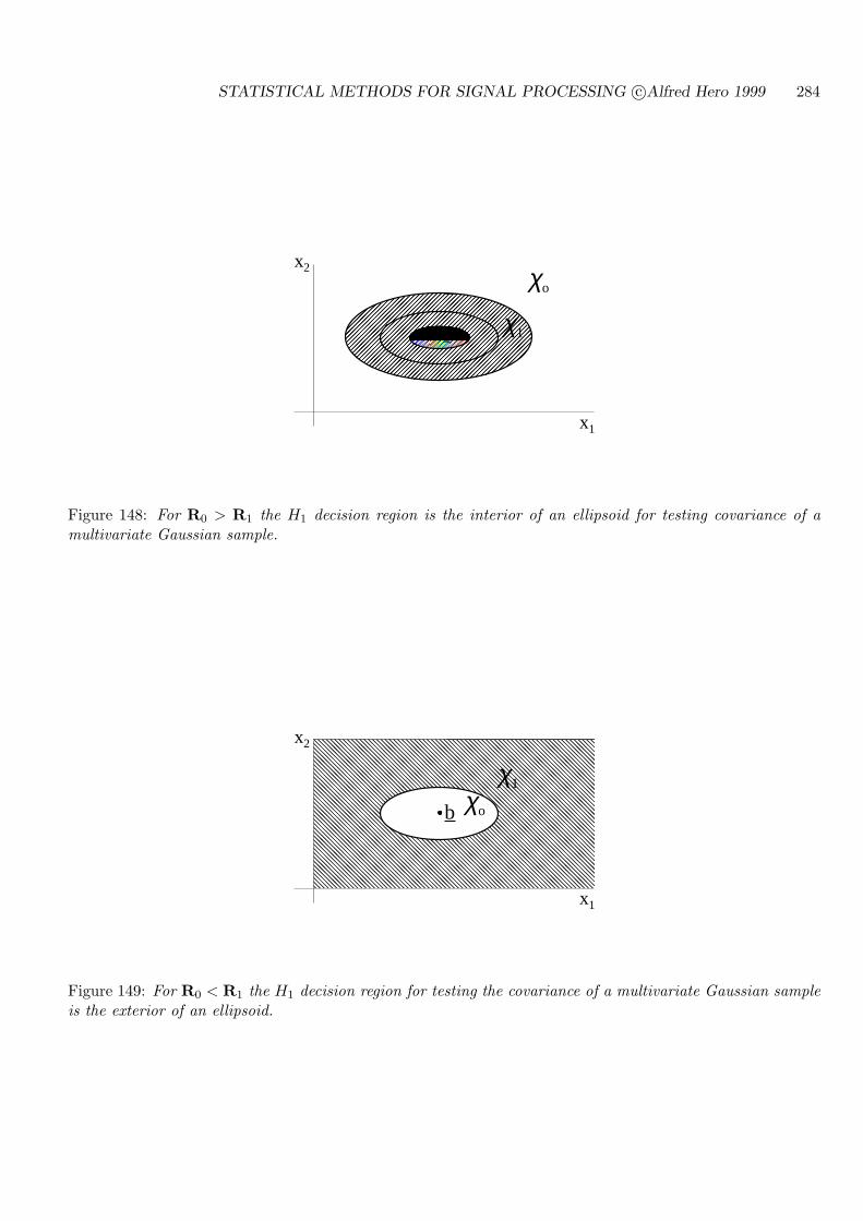
STATISTICAL METHODS FOR SIGNAL PROCESSING c©Alfred Hero 1999 284
χ1
χo
x2
x1
b
Figure 148: For R0 > R1 the H1 decision region is the interior of an ellipsoid for testing covariance of amultivariate Gaussian sample.
χ1
χo
x1
b
x2
Figure 149: For R0 < R1 the H1 decision region for testing the covariance of a multivariate Gaussian sampleis the exterior of an ellipsoid.
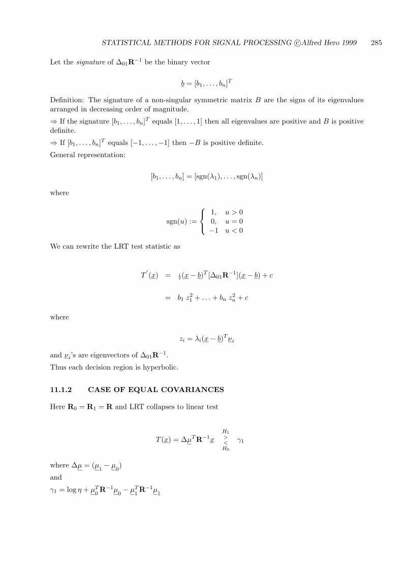
STATISTICAL METHODS FOR SIGNAL PROCESSING c©Alfred Hero 1999 285
Let the signature of ∆01R−1 be the binary vector
b = [b1, . . . , bn]T
Definition: The signature of a non-singular symmetric matrix B are the signs of its eigenvaluesarranged in decreasing order of magnitude.
⇒ If the signature [b1, . . . , bn]T equals [1, . . . , 1] then all eigenvalues are positive and B is positivedefinite.
⇒ If [b1, . . . , bn]T equals [−1, . . . ,−1] then −B is positive definite.
General representation:
[b1, . . . , bn] = [sgn(λ1), . . . , sgn(λn)]
where
sgn(u) :=
1, u > 00, u = 0−1 u < 0
We can rewrite the LRT test statistic as
T′(x) = 1
2(x− b)T [∆01R−1](x− b) + c
= b1 z21 + . . . + bn z2
n + c
where
zi = λi(x− b)T νi
and νi’s are eigenvectors of ∆01R−1.
Thus each decision region is hyperbolic.
11.1.2 CASE OF EQUAL COVARIANCES
Here R0 = R1 = R and LRT collapses to linear test
T (x) = ∆µTR−1xH1
><H0
γ1
where ∆µ = (µ1− µ
0)
and
γ1 = log η + µT0R−1µ
0− µT
1R−1µ
1
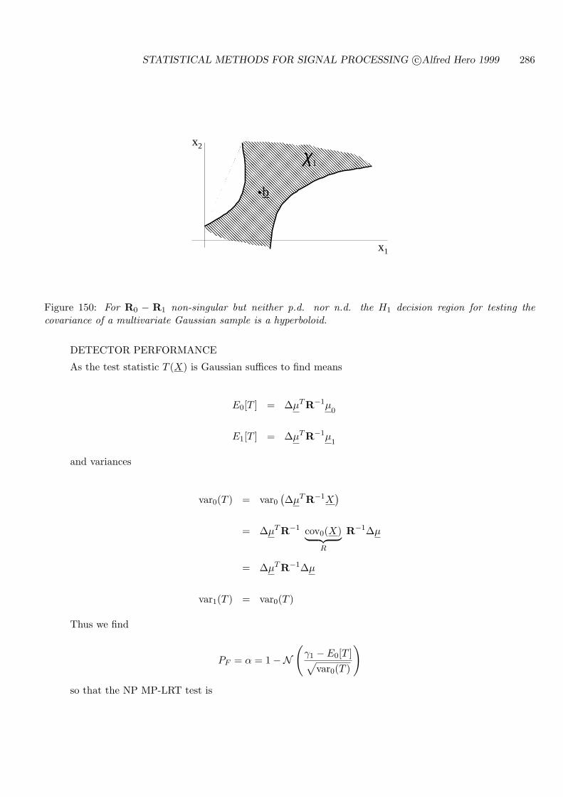
STATISTICAL METHODS FOR SIGNAL PROCESSING c©Alfred Hero 1999 286
χ1
x1
b
x2
Figure 150: For R0 − R1 non-singular but neither p.d. nor n.d. the H1 decision region for testing thecovariance of a multivariate Gaussian sample is a hyperboloid.
DETECTOR PERFORMANCE
As the test statistic T (X) is Gaussian suffices to find means
E0[T ] = ∆µTR−1µ0
E1[T ] = ∆µTR−1µ1
and variances
var0(T ) = var0(∆µTR−1X
)
= ∆µTR−1 cov0(X)︸ ︷︷ ︸R
R−1∆µ
= ∆µTR−1∆µ
var1(T ) = var0(T )
Thus we find
PF = α = 1−N(
γ1 − E0[T ]√var0(T )
)
so that the NP MP-LRT test is

STATISTICAL METHODS FOR SIGNAL PROCESSING c©Alfred Hero 1999 287
∆µTR−1xH1
><H0
√∆µTR−1∆µ N−1(1− α) + ∆µTR−1µ
0
or equivalently
∆µTR−1(x− µ0)√
∆µTR−1∆µ
H1
><H0
N−1(1− α)
NOTES:
1. For µ06= 0: MP test is not UMP w.r.t unknown parameter variations
2. For µ0
= 0: MP test is UMP w.r.t. constant positive scaling of µ1
Next find power:
PD = β = 1−N(
γ1 − E1[T ]√var1(T )
)
giving ROC curve:
β = 1−N (N−1 (1− α)− d)
where d is detectability index
d =E1[T ]−E0[T ]√
var0(T )
=√
∆µTR−1∆µ
Example 44 Detection of known signal in white noise
H0 : xk = wk
k = 1, . . . , n
H1 : xk = sk + wk
* w ∼ Nn(0, σ2I),
* s and σ2 known
Identify:
µ0
= 0, ∆µ = s, R = σ2I
so that the LRT takes the form of a matched filter
STATISTICAL METHODS FOR SIGNAL PROCESSING c©Alfred Hero 1999 288
T (x) = sT x =n∑
k=1
skxk
H1
><H0
γ
γ = σ2 log η − ‖s‖2
GEOMETRIC INTERPRETATION
The LRT can be expressed geometrically as a signal ”projection” detector
Projection of x onto s is
x =[
s sT
‖s‖2
]
︸ ︷︷ ︸Πs
x
= ssT x
‖s‖2
= s< s, x >
‖s‖2
︸ ︷︷ ︸Proj. coef.
Length of this projection is
‖x‖ = ‖s‖∣∣∣∣sT x
‖s‖2
∣∣∣∣
= |T (x)| 1‖s‖
Conclude:
* LRT is a threshold test on the projection coefficient of the orthogonal projection of x onto s
* LRT is threshold test on ”signed length” of x
* LRT is related to LLS estimator x of x given s
PERFORMANCE
Equivalently, for MP test of level α we have
sT x
‖s‖ σ
H1
><H0
N−1(1− α)
This test is UMP relative to signal energy ‖s‖2
Now compute detectability index:
d2 = ‖s‖2/σ2 =∑n
k=1 s2k
σ2=: SNR (111)

STATISTICAL METHODS FOR SIGNAL PROCESSING c©Alfred Hero 1999 289
x
s
x
Figure 151: MP detector applies a threshold to projection coefficient < x, s > /‖s‖2 of orthogonal projectionof x onto s, shown here for the case of n = 2.
Compute LLS projection
coefficient
Ho
H1
> <x
s
< s, x>
|| s || 2
Figure 152: MP detector block diagram implemented with a LLS estimator of x.
STATISTICAL METHODS FOR SIGNAL PROCESSING c©Alfred Hero 1999 290
NOTE:
* detection index is invariant to shape of waveform s.
* detector power only depends on total signal-to-noise ratio (SNR).
Note: two ways to implement optimal detector
Cross-correlator:
Matched Filter:
Example 45 Detection of known signal in non-white noise:
H0 : xk = wk
k = 1, . . . , n
H1 : xk = sk + wk
* w ∼ Nn(0,R), R not scaled identity.
Optimal detector
T (x) =sTR−1x√sTR−1s
H1
><H0
N−1(1− α)
Q. How to modularize detector?
A. transform to the white noise case via preprocessing with matrix H
Produces white noise measurements
x = H · x
We will require matrix filter H to have properties:
1. cov0(x) = cov1(x) = I: ⇒ whitening property
2. H is invertible matrix: ⇒ output remains sufficient statistic
MATRIX FACTORIZATION
For any symmetric positive definite covariance matrix R there exists a positive definite squareroot factor R 1
2 and a positive definite inverse factor R− 12 which satisfy:
R = R12 R
12 , and R−1 = R− 1
2 R− 12 .
There are many possible factorizations of this type. We have already seen the Cholesky factoriza-tion in Chapter 6 which yields upper and lower triangular factors. Here we focus on a symmetricfactorization given by the eigendecomposition of R = UDUT , where
* D = diag(λi) are (positive) eigenvalues of R
* U = [ν1, . . . , νp] are (orthogonal) eigenvectors of R
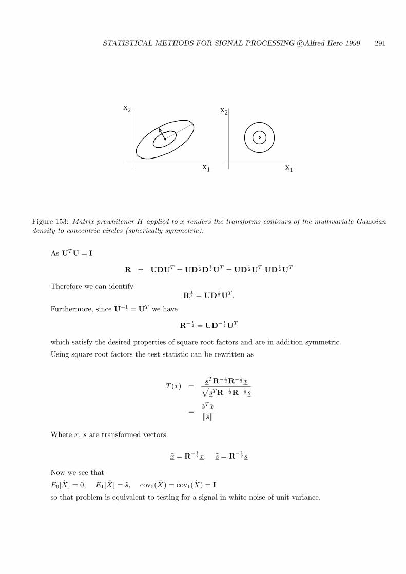
STATISTICAL METHODS FOR SIGNAL PROCESSING c©Alfred Hero 1999 291
x1x1
x2x2
Figure 153: Matrix prewhitener H applied to x renders the transforms contours of the multivariate Gaussiandensity to concentric circles (spherically symmetric).
As UTU = I
R = UDUT = UD12 D
12 UT = UD
12 UT UD
12 UT
Therefore we can identifyR
12 = UD
12 UT .
Furthermore, since U−1 = UT we have
R− 12 = UD− 1
2 UT
which satisfy the desired properties of square root factors and are in addition symmetric.
Using square root factors the test statistic can be rewritten as
T (x) =sTR− 1
2 R− 12 x√
sTR− 12 R− 1
2 s
=sT x
‖s‖
Where x, s are transformed vectors
x = R− 12 x, s = R− 1
2 s
Now we see that
E0[X] = 0, E1[X] = s, cov0(X) = cov1(X) = I
so that problem is equivalent to testing for a signal in white noise of unit variance.
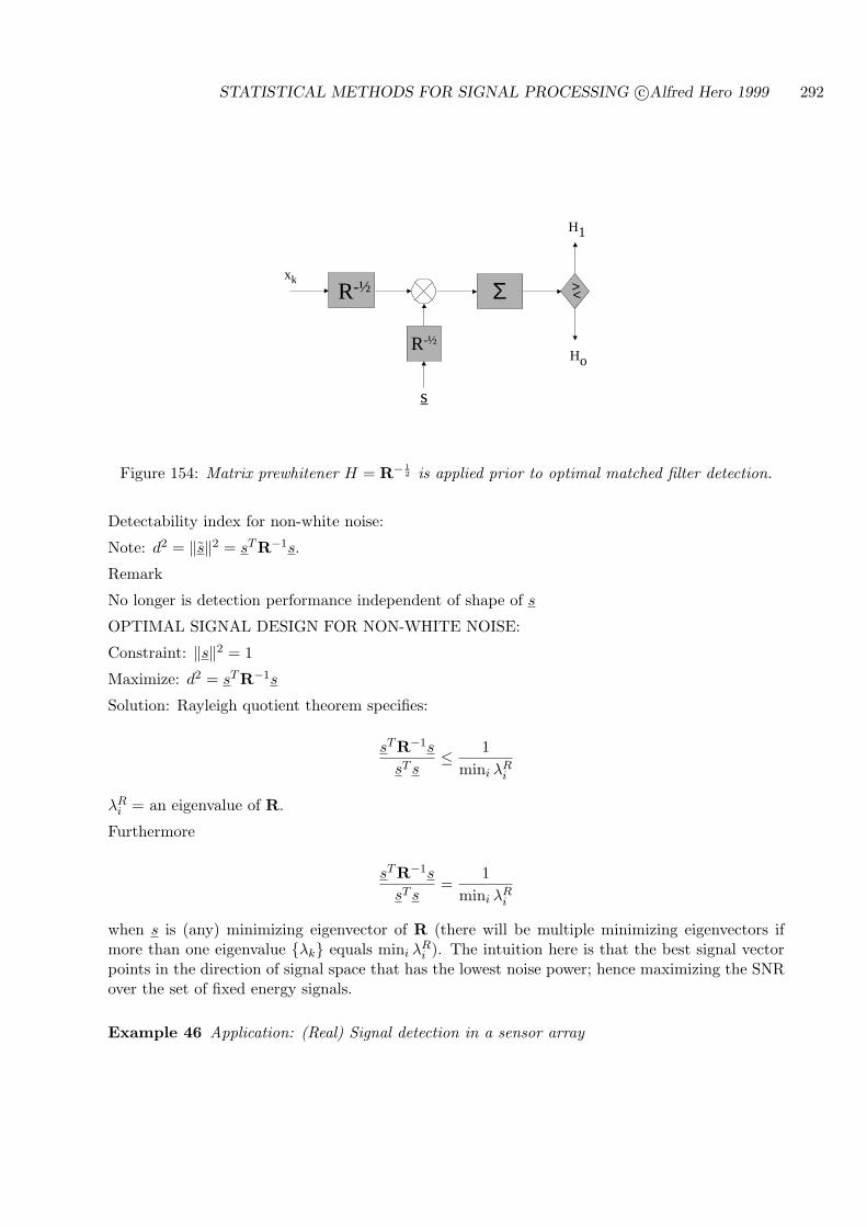
STATISTICAL METHODS FOR SIGNAL PROCESSING c©Alfred Hero 1999 292
R-½
Ho
H1
> < xk
Σ
R-½
s
Figure 154: Matrix prewhitener H = R− 12 is applied prior to optimal matched filter detection.
Detectability index for non-white noise:
Note: d2 = ‖s‖2 = sTR−1s.
Remark
No longer is detection performance independent of shape of s
OPTIMAL SIGNAL DESIGN FOR NON-WHITE NOISE:
Constraint: ‖s‖2 = 1
Maximize: d2 = sTR−1s
Solution: Rayleigh quotient theorem specifies:
sTR−1s
sT s≤ 1
mini λRi
λRi = an eigenvalue of R.
Furthermore
sTR−1s
sT s=
1mini λR
i
when s is (any) minimizing eigenvector of R (there will be multiple minimizing eigenvectors ifmore than one eigenvalue λk equals mini λ
Ri ). The intuition here is that the best signal vector
points in the direction of signal space that has the lowest noise power; hence maximizing the SNRover the set of fixed energy signals.
Example 46 Application: (Real) Signal detection in a sensor array
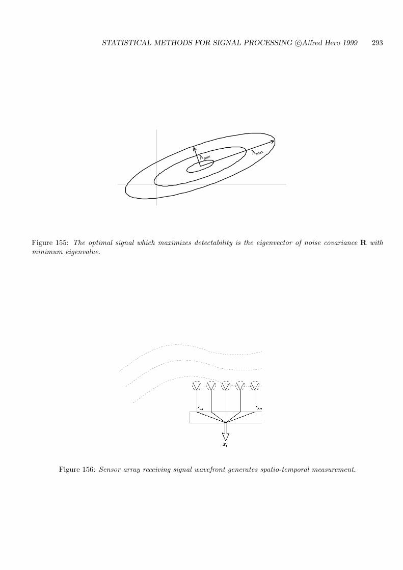
STATISTICAL METHODS FOR SIGNAL PROCESSING c©Alfred Hero 1999 293
λminλmax
Figure 155: The optimal signal which maximizes detectability is the eigenvector of noise covariance R withminimum eigenvalue.
Figure 156: Sensor array receiving signal wavefront generates spatio-temporal measurement.
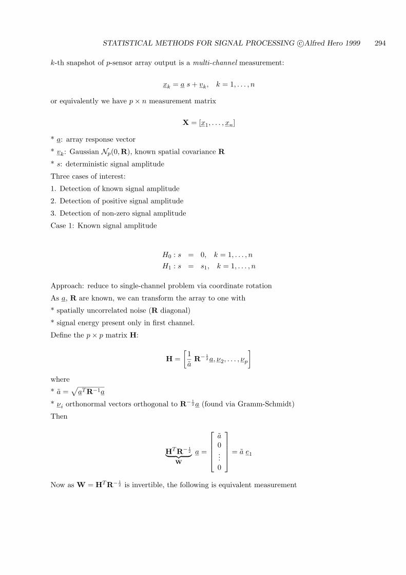
STATISTICAL METHODS FOR SIGNAL PROCESSING c©Alfred Hero 1999 294
k-th snapshot of p-sensor array output is a multi-channel measurement:
xk = a s + vk, k = 1, . . . , n
or equivalently we have p× n measurement matrix
X = [x1, . . . , xn]
* a: array response vector
* vk: Gaussian Np(0,R), known spatial covariance R
* s: deterministic signal amplitude
Three cases of interest:
1. Detection of known signal amplitude
2. Detection of positive signal amplitude
3. Detection of non-zero signal amplitude
Case 1: Known signal amplitude
H0 : s = 0, k = 1, . . . , n
H1 : s = s1, k = 1, . . . , n
Approach: reduce to single-channel problem via coordinate rotation
As a, R are known, we can transform the array to one with
* spatially uncorrelated noise (R diagonal)
* signal energy present only in first channel.
Define the p× p matrix H:
H =[1a
R− 12 a, ν2, . . . , νp
]
where
* a =√
aTR−1a
* νi orthonormal vectors orthogonal to R− 12 a (found via Gramm-Schmidt)
Then
HTR− 12︸ ︷︷ ︸
W
a =
a0...0
= a e1
Now as W = HTR− 12 is invertible, the following is equivalent measurement
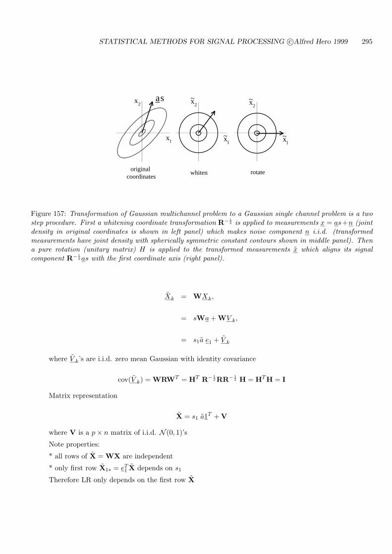
STATISTICAL METHODS FOR SIGNAL PROCESSING c©Alfred Hero 1999 295
1x
2x
1x~
2x~
2x~
1x~
original coordinates
whiten rotate
a s
Figure 157: Transformation of Gaussian multichannel problem to a Gaussian single channel problem is a twostep procedure. First a whitening coordinate transformation R− 1
2 is applied to measurements x = as+n (jointdensity in original coordinates is shown in left panel) which makes noise component n i.i.d. (transformedmeasurements have joint density with spherically symmetric constant contours shown in middle panel). Thena pure rotation (unitary matrix) H is applied to the transformed measurements x which aligns its signalcomponent R− 1
2 as with the first coordinate axis (right panel).
Xk = WXk,
= sWa + WV k,
= s1a e1 + V k
where V k’s are i.i.d. zero mean Gaussian with identity covariance
cov(V k) = WRWT = HT R− 12 RR− 1
2 H = HTH = I
Matrix representation
X = s1 a1T + V
where V is a p× n matrix of i.i.d. N (0, 1)’s
Note properties:
* all rows of X = WX are independent
* only first row X1∗ = eT1 X depends on s1
Therefore LR only depends on the first row X
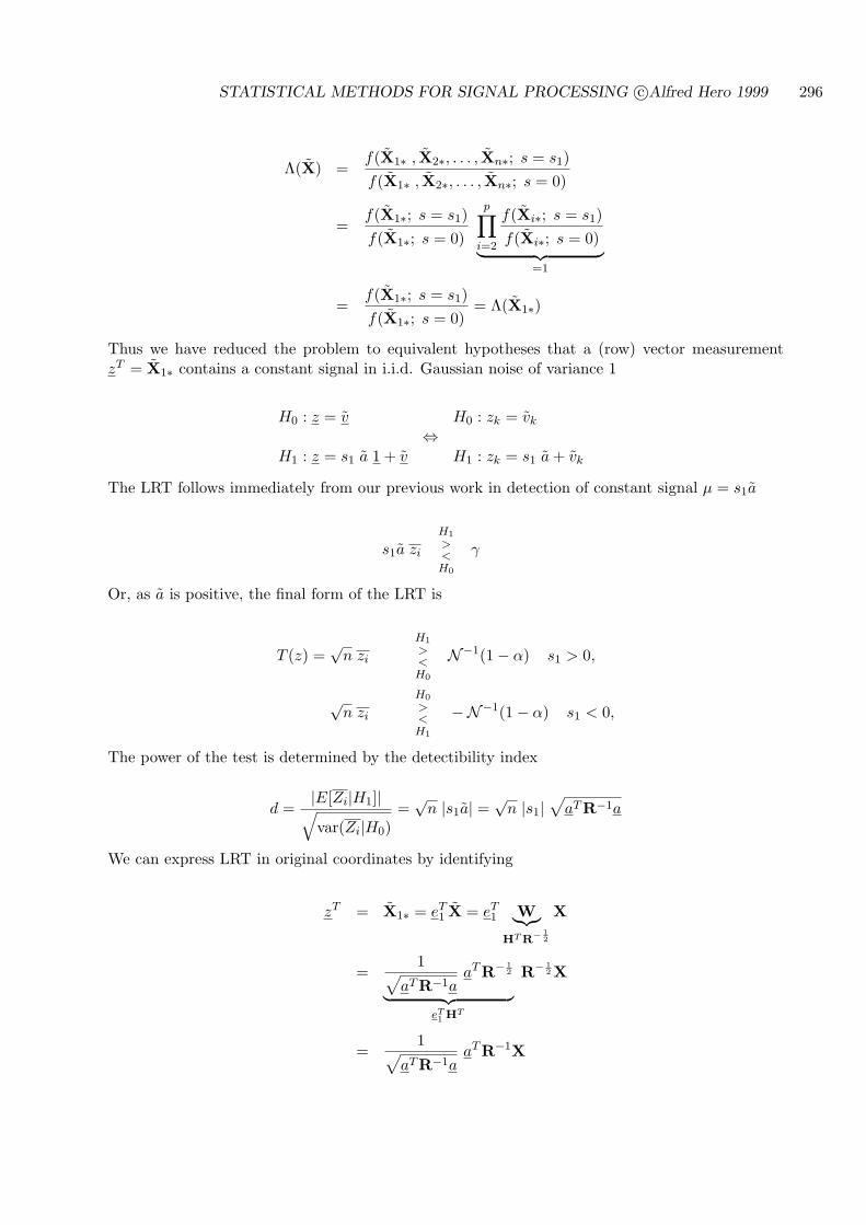
STATISTICAL METHODS FOR SIGNAL PROCESSING c©Alfred Hero 1999 296
Λ(X) =f(X1∗ , X2∗, . . . , Xn∗; s = s1)f(X1∗ , X2∗, . . . , Xn∗; s = 0)
=f(X1∗; s = s1)f(X1∗; s = 0)
p∏
i=2
f(Xi∗; s = s1)f(Xi∗; s = 0)
︸ ︷︷ ︸=1
=f(X1∗; s = s1)f(X1∗; s = 0)
= Λ(X1∗)
Thus we have reduced the problem to equivalent hypotheses that a (row) vector measurementzT = X1∗ contains a constant signal in i.i.d. Gaussian noise of variance 1
H0 : z = v H0 : zk = vk
⇔H1 : z = s1 a 1 + v H1 : zk = s1 a + vk
The LRT follows immediately from our previous work in detection of constant signal µ = s1a
s1a zi
H1
><H0
γ
Or, as a is positive, the final form of the LRT is
T (z) =√
n zi
H1
><H0
N−1(1− α) s1 > 0,
√n zi
H0
><H1
−N−1(1− α) s1 < 0,
The power of the test is determined by the detectibility index
d =|E[Zi|H1]|√var(Zi|H0)
=√
n |s1a| =√
n |s1|√
aTR−1a
We can express LRT in original coordinates by identifying
zT = X1∗ = eT1 X = eT
1 W︸︷︷︸HT R−
12
X
=1√
aTR−1aaTR− 1
2
︸ ︷︷ ︸eT1 HT
R− 12 X
=1√
aTR−1aaTR−1X
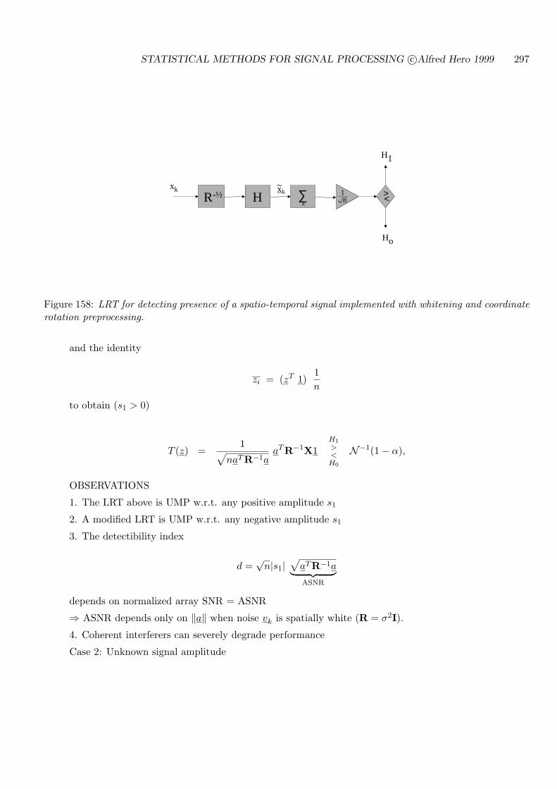
STATISTICAL METHODS FOR SIGNAL PROCESSING c©Alfred Hero 1999 297
kx~ xk
R-½
Ho
H1
> <n1H ∑
k
Figure 158: LRT for detecting presence of a spatio-temporal signal implemented with whitening and coordinaterotation preprocessing.
and the identity
zi = (zT 1)1n
to obtain (s1 > 0)
T (z) =1√
naTR−1aaTR−1X1
H1
><H0
N−1(1− α),
OBSERVATIONS
1. The LRT above is UMP w.r.t. any positive amplitude s1
2. A modified LRT is UMP w.r.t. any negative amplitude s1
3. The detectibility index
d =√
n|s1|√
aTR−1a︸ ︷︷ ︸ASNR
depends on normalized array SNR = ASNR
⇒ ASNR depends only on ‖a‖ when noise vk is spatially white (R = σ2I).
4. Coherent interferers can severely degrade performance
Case 2: Unknown signal amplitude
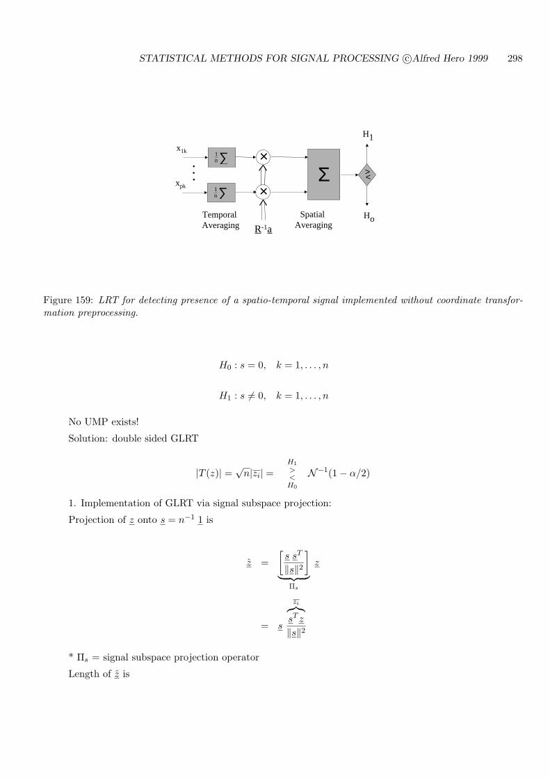
STATISTICAL METHODS FOR SIGNAL PROCESSING c©Alfred Hero 1999 298
H1
Ho
> <
x1k
∑ n1 ×
Σ xpk
∑ n1 ×
R-1a
Temporal Averaging
Spatial Averaging
• • •
Figure 159: LRT for detecting presence of a spatio-temporal signal implemented without coordinate transfor-mation preprocessing.
H0 : s = 0, k = 1, . . . , n
H1 : s 6= 0, k = 1, . . . , n
No UMP exists!
Solution: double sided GLRT
|T (z)| = √n|zi| =
H1
><H0
N−1(1− α/2)
1. Implementation of GLRT via signal subspace projection:
Projection of z onto s = n−1 1 is
z =[
s sT
‖s‖2
]
︸ ︷︷ ︸Πs
z
= s
zi︷︸︸︷sT z
‖s‖2
* Πs = signal subspace projection operator
Length of z is
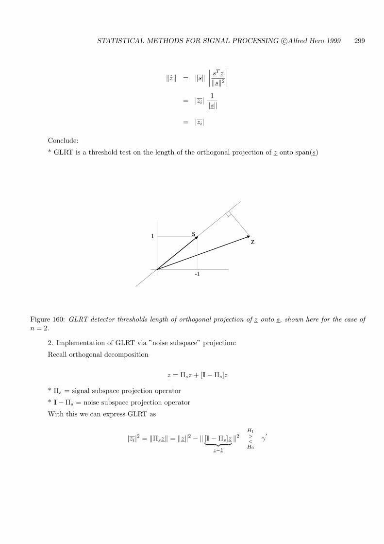
STATISTICAL METHODS FOR SIGNAL PROCESSING c©Alfred Hero 1999 299
‖z‖ = ‖s‖∣∣∣∣sT z
‖s‖2
∣∣∣∣
= |zi| 1‖s‖
= |zi|
Conclude:
* GLRT is a threshold test on the length of the orthogonal projection of z onto span(s)
1
-1
zs
Figure 160: GLRT detector thresholds length of orthogonal projection of z onto s, shown here for the case ofn = 2.
2. Implementation of GLRT via ”noise subspace” projection:
Recall orthogonal decomposition
z = Πsz + [I−Πs]z
* Πs = signal subspace projection operator
* I−Πs = noise subspace projection operator
With this we can express GLRT as
|zi|2 = ‖Πsz‖ = ‖z‖2 − ‖ [I−Πs]z︸ ︷︷ ︸z−z
‖2H1
><H0
γ′
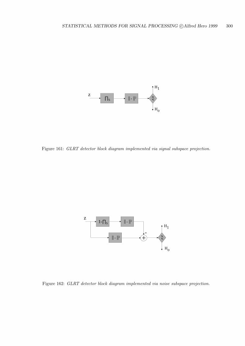
STATISTICAL METHODS FOR SIGNAL PROCESSING c©Alfred Hero 1999 300
Ho
H1
> < z
|| • ||2∏S
Figure 161: GLRT detector block diagram implemented via signal subspace projection.
Ho
H1
> <
|| • ||2
z|| • ||21-∏S
+-
Figure 162: GLRT detector block diagram implemented via noise subspace projection.
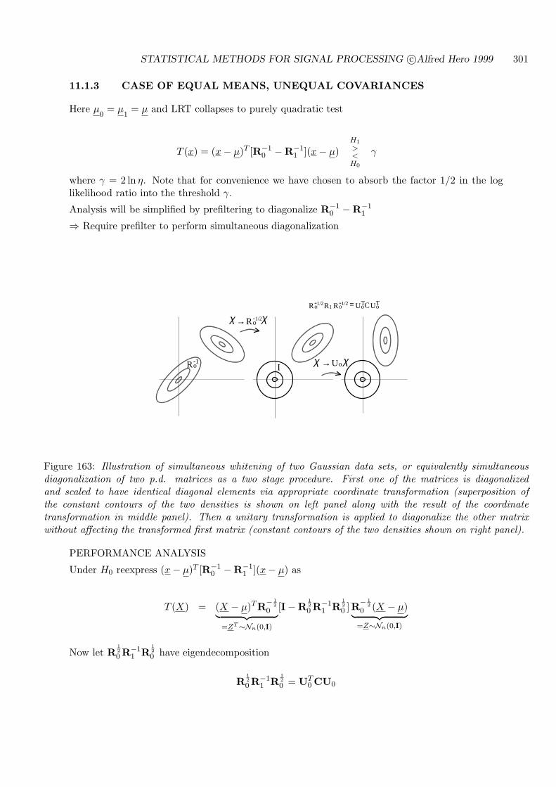
STATISTICAL METHODS FOR SIGNAL PROCESSING c©Alfred Hero 1999 301
11.1.3 CASE OF EQUAL MEANS, UNEQUAL COVARIANCES
Here µ0
= µ1
= µ and LRT collapses to purely quadratic test
T (x) = (x− µ)T [R−10 −R−1
1 ](x− µ)H1
><H0
γ
where γ = 2 ln η. Note that for convenience we have chosen to absorb the factor 1/2 in the loglikelihood ratio into the threshold γ.
Analysis will be simplified by prefiltering to diagonalize R−10 −R−1
1
⇒ Require prefilter to perform simultaneous diagonalization
R 1-o
R 1/2-o→ χχ
I Uo→ χχ
U U R- RR - To
Tooo
1/21
1/2 = C
Figure 163: Illustration of simultaneous whitening of two Gaussian data sets, or equivalently simultaneousdiagonalization of two p.d. matrices as a two stage procedure. First one of the matrices is diagonalizedand scaled to have identical diagonal elements via appropriate coordinate transformation (superposition ofthe constant contours of the two densities is shown on left panel along with the result of the coordinatetransformation in middle panel). Then a unitary transformation is applied to diagonalize the other matrixwithout affecting the transformed first matrix (constant contours of the two densities shown on right panel).
PERFORMANCE ANALYSIS
Under H0 reexpress (x− µ)T [R−10 −R−1
1 ](x− µ) as
T (X) = (X − µ)TR− 12
0︸ ︷︷ ︸=ZT∼Nn(0,I)
[I−R120 R−1
1 R120 ]R− 1
20 (X − µ)︸ ︷︷ ︸
=Z∼Nn(0,I)
Now let R120 R−1
1 R120 have eigendecomposition
R120 R−1
1 R120 = UT
0 CU0
STATISTICAL METHODS FOR SIGNAL PROCESSING c©Alfred Hero 1999 302
* U0 orthogonal matrix of eigenvectors
* C = diag(c1, . . . , cn) diagonal matrix of eigenvalues.
T (X) = (U0Z)T
︸ ︷︷ ︸Nn(0,I)
[I−C] (U0Z)︸ ︷︷ ︸Nn(0,I)
= n(1− c)∑
i
Z2i (1− ci)∑j(1− cj)
︸ ︷︷ ︸Chi−sq.−mixture
where
(1− c) = n−1∑
i
(1− ci)
There are two cases to consider: 0 < ci < 1 vs ci > 1. Note that consideration of ci = 0 is notrequired since we have assumed that R1 and R0 are positive definite matrices.
CASE 1: 0 < ci < 1 for all i
Here
(1− c) > 0
so we can absorb it into into threshold γ
This gives MP level α test in terms of orthogonalized measurements zi
∑
i
z2i (1− ci)∑j(1− cj)
H1
><H0
χ−1n,1−c(1− α)
Finally, retracing our steps to the original observables we have the implementable level α LRT test
(x− µ)T (R−10 −R−1
1 )(x− µ)H1
><H0
aχ−1n,1−c(1− α).
Here a =∑n
i=1(1−ci) and χn,1−c is the CDF of Chi-square-mixture r.v. with n degrees of freedomand mixture parameter vector
1− c = [1− c1, . . . , 1− cn]T
(Johnson, Kotz and Balakrishnan [30, Sec. 18.8]).
It remains to find the power:
In a similar manner, under H1 we can express
T (X) = (X − µ)TR− 12
1 [R121 R−1
0 R121 − I]R− 1
21 (X − µ)
= (U1Z)T [C−1 − I](U1Z)
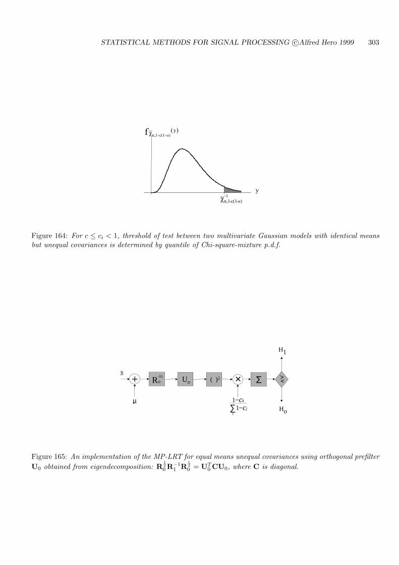
STATISTICAL METHODS FOR SIGNAL PROCESSING c©Alfred Hero 1999 303
)(f )-c(1-n,1y
y1
)-c(1-n,1
Figure 164: For c ≤ ci < 1, threshold of test between two multivariate Gaussian models with identical meansbut unequal covariances is determined by quantile of Chi-square-mixture p.d.f.
Ho
H1
> <x
R½-o ×+
µ
Uo ( )2 Σ
1 kc−
j∑ jc−1
Figure 165: An implementation of the MP-LRT for equal means unequal covariances using orthogonal prefilterU0 obtained from eigendecomposition: R
120 R−1
1 R120 = UT
0 CU0, where C is diagonal.

STATISTICAL METHODS FOR SIGNAL PROCESSING c©Alfred Hero 1999 304
= n(1/c− 1)∑
i
Z2i (1/ci − 1)∑j(1/cj − 1)
︸ ︷︷ ︸Chi−sq.−mixture
where U1 in the above is an orthogonal matrix.
As (1/c− 1) > 0, we easily obtain power as:
β = 1− χn,1/c−1(ρ χ−1n,1−c(1− α))
where
ρ = (1− c)/(1/c− 1)
)(f $ c-n,1y
)(f $ 1-n,1/cy
c = 0.3n = 3
$ 1)-c(1-n,1
−. PFA
y
Figure 166: For c ≤ ci < 1 ROC of test between two multivariate Gaussian models with identical means butunequal covariances is determined by upper quantiles of pair of Chi-square-mixture p.d.f.’s
CASE 2: ci > 1 for all i
Here we have (1− c) < 0 and the constant in the test can be absorbed into threshold only withchange of the inequalities.
Obtain the MP level α test in zi coordinates
∑
i
z2i (1− ci)∑j(1− cj)
H0
><H1
χ−1n,1−c(α)
and, using similar arguments as before, we obtain power curve
β = χn,1/c−1(ρ χ−1n,1−c(α))
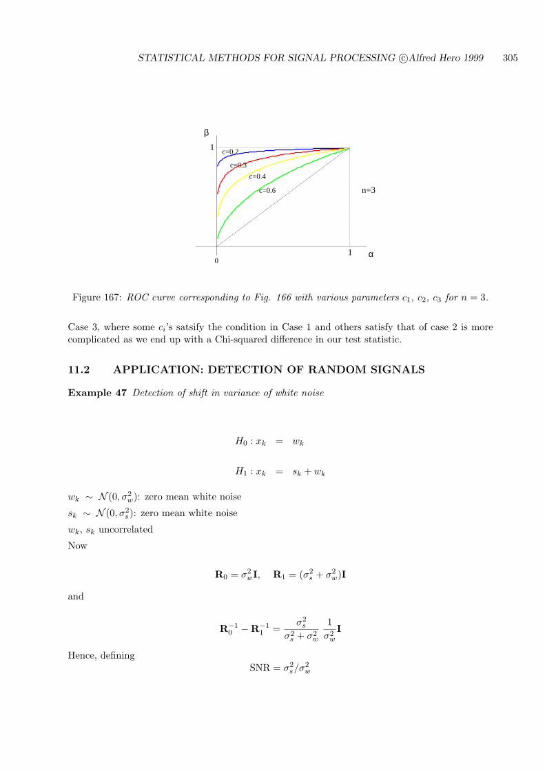
STATISTICAL METHODS FOR SIGNAL PROCESSING c©Alfred Hero 1999 305
β
α
1
1
c=0.2
c=0.3
c=0.4
c=0.6 n=3
0
Figure 167: ROC curve corresponding to Fig. 166 with various parameters c1, c2, c3 for n = 3.
Case 3, where some ci’s satsify the condition in Case 1 and others satisfy that of case 2 is morecomplicated as we end up with a Chi-squared difference in our test statistic.
11.2 APPLICATION: DETECTION OF RANDOM SIGNALS
Example 47 Detection of shift in variance of white noise
H0 : xk = wk
H1 : xk = sk + wk
wk ∼ N (0, σ2w): zero mean white noise
sk ∼ N (0, σ2s): zero mean white noise
wk, sk uncorrelated
Now
R0 = σ2wI, R1 = (σ2
s + σ2w)I
and
R−10 −R−1
1 =σ2
s
σ2s + σ2
w
1σ2
w
I
Hence, definingSNR = σ2
s/σ2w
STATISTICAL METHODS FOR SIGNAL PROCESSING c©Alfred Hero 1999 306
ci is the constant
ci = σ2w/(σ2
w + σ2s) = 1/(1 + SNR)
1− ci = SNR/(1 + SNR)1/ci − 1 = 1/SNR
ρ = (1− c)/(1/c− 1) = 1/(1 + SNR)
Note the SNR is defined differently in the case of a zero mean stochastic signal and a non-zeromean deterministic signal (111).
INTERPRETATION: 1 − ci is the temporal “coherency function” (SNR normalized to interval[0, 1])) of the signal w.r.t. the measurement
κ := σ2s/(σ2
w + σ2s) = SNR/(1 + SNR)
Thus LRT reduces to
T (x) =κ
σ2w
n∑
k=1
x2k
H1
><H0
γ
Which reduces to the Chi-squared test (“energy detector”)
T′(x) =
n∑
k=1
x2k/σ2
w
H1
><H0
χ−1n (1− α)
NOTE: relation between Chi-square-mixture and Chi-square CDF’s when 1− ci = constant
χn,(1−c)
= n−1χn
Power curve reduces to
β = 1− χn
(1
1 + SNRχ−1
n (1− α))
Example 48 Detection of uncorrelated non-stationary signal in noise
H0 : xk = wk
H1 : xk = sk + wk
wk ∼ N (0, σ2w(k)): uncorrelated noise samples
sk ∼ N (0, σ2s(k)): uncorrelated signal samples
STATISTICAL METHODS FOR SIGNAL PROCESSING c©Alfred Hero 1999 307
wk, sk uncorrelated
In this case
R0 = diag(σ2w(i)), R1 = diag(σ2
s(i) + σ2w(i))
and
R−10 −R−1
1 = diag(
σ2s(i)
σ2s(i) + σ2
w(i)1
σ2w(i)
)
= diag(κi/σ2
w(i))
where κi is time varying coherency function
κi =σ2
s(i)σ2
s(i) + σ2w(i)
is
Hence, MP-LRT of level α reduces to
1κ
n∑
k=1
κkx2
k
σ2w(k)
H1
><H0
= χ−1n,κ(1− α)
or equivalently in terms of the original T (x)
T (x) =n∑
k=1
κkx2
k
σ2w(k)
H1
><H0
γ = κ χ−1n,κ(1− α)
Special case of white noise: σ2w(k) = No/2
n∑
k=1
κk x2k
H1
><H0
γ =No
2κ χ−1
n,κ(1− α)
TWO USEFUL INTERPRETATIONS
Assume white noise for simplicity (we know that we can simply prewhiten by 1/σw(k) if non-whitewk).
1. “MEMORYLESS” ESTIMATOR CORRELATOR IMPLEMENTATION
Rewrite test statistic as
n∑
k=1
sk xk
H1
><H0
γ
where sk is LLMSE estimator of sk given xk
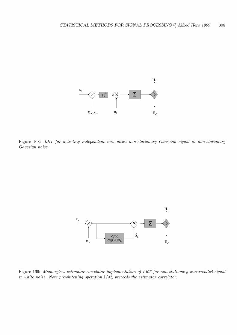
STATISTICAL METHODS FOR SIGNAL PROCESSING c©Alfred Hero 1999 308
Ho
H1
><xk
Σ
σw(k)
×
κk
( )2
Figure 168: LRT for detecting independent zero mean non-stationary Gaussian signal in non-stationaryGaussian noise.
Ho
H1
><xk
Σ×
22 2
ws
s11
1 (k)
(k)+
kS
w1
Figure 169: Memoryless estimator correlator implementation of LRT for non-stationary uncorrelated signalin white noise. Note prewhitening operation 1/σ2
w preceeds the estimator correlator.

STATISTICAL METHODS FOR SIGNAL PROCESSING c©Alfred Hero 1999 309
sk =σ2
s(k)σ2
s(k) + σ2w
xk = κk xk
2. “MEMORYLESS” FILTER-SQUARER IMPLEMENTATION
Rewrite test statistic as
n∑
k=1
y2k
H1
><H0
γ
where yk is defined as
yk =
√σ2
s(k)σ2
s(k) + σ2w
xk =√
κi xk
Ho
H1
><Σ22 2
ws
s11
1 (k)
(k)+ ( )2
w1
xk
Figure 170: Memoryless filter squarer implementation of LRT for non-stationary uncorrelated signal in whitenoise.
POWER OF MEMORYLESS ESTIMATOR CORRELATOR:
as above
β = 1− χn,1/c−1(ρχ−1n,1−c(1− α))
where
ci =σ2
w
(σ2s(i) + σ2
w)= 1− κi
ρ =∑
i κi∑i κi/(1− κi)
STATISTICAL METHODS FOR SIGNAL PROCESSING c©Alfred Hero 1999 310
To a good approximation, at high SNR it can be shown that ROC depends on n, No, σ2s(i) only
through the following three SNR moments
SNR(1) =1
σ2w
n∑
i=1
σ2s(i)
SNR(2) =(
1σ2
w
)2 n∑
i,j=1
σ2s(i)σ
2s(j)
SNR(3) =(
1σ2
w
)3 n∑
i,j,k=1
σ2s(i)σ
2s(j)σ
2s(k)
Example 49 Offline detection of w.s.s. signal in white noise
Assume a window of n samples of a zero mean w.s.s. process xk are available to test
H0 : xk = wk, k = 0, . . . , n− 1H1 : xk = sk + wk k = 0, . . . , n− 1
where
* wk: Gaussian white noise with PSD Pw(ω) = No/2
* sk: zero mean w.s.s. Gaussian signal with known autocorrelation function rs(k) = E[slsl−k]
* wk, sk uncorrelated
The n× n covariance matrices under H0 and H1 are
R0 = Rw = σ2wI, R1 = Rs + σ2
wI
where Rs = (( rs(l −m) ))nl,m=1 is an n× n p.d. Toeplitz matrix and σ2
w = No/2.
We know that MP-LRT is of form
T (x) = xT (R−10 −R−1
1 )xH1
><H0
η
However, in this form, the detector is not implementable for large n due to the need for to performthe Rs matrix inversion. An alternative, for large n, is to invoke a “spectral decomposition” ofthe Toeplitz matrix Rs, sometimes known as the Grenander representation, pursued below.
Define E the n× n unitary “DFT matrix” with n columns ek given by
ek = [1, ejωk , . . . , ejωk(n−1)]T /√
n
j =√−1, and ωk = k
n2π ∈ [0, 2π), k = 0, . . . , n − 1, is the k-th radian frequency. Letx = [x1, . . . , xn]T denote the vector of (
√n-normalized) DFT coefficients associated with x =
[x1, . . . , xn]T :x = EHx.

STATISTICAL METHODS FOR SIGNAL PROCESSING c©Alfred Hero 1999 311
Then as EEH = I, we can represent the LRT statistic as
xT (R−10 −R−1
1 )x = [EHx]H(EHR−10 E−EHR−1
1 E)[EHx]
= xH(1
σ2w
I−EHR−11 E)x (112)
Now, remarkably, for large n the matrix EHR−11 E is approximately diagonal, i.e. the DFT operator
E diagonalizes the covariance matrix. To show this we first state a theorem:
Spectral approximation Theorem [11]: For any positive definite Toeplitz matrix R = ((ri−j))ni,j=1
EHRE = diagk(DFTr(ωk)) + O(1/n)
where DFTr(ωk) =∑n−1
k=−n+1 rke−jωk is the k-th coefficient of the discrete fourier transform (DFT)
of the sequence r = r−n+1, . . . , r0, . . . , rn−1, and O(1/n) is a term that goes to zero at rate 1/n.This implies that for large n the eigenvectors of R are the DFT vectors and the eigenvalues arethe DFT coefficients of the distinct elements of R.
Proof of spectral approximation theorem:
It suffices to show that as n →∞ the DFT matrix E asymptotically diagonalizes R, i.e.,
eHk Rel →
DFTr(ωk), k = l
0, o.w.
So let’s write out the quadratic form explicitly
eHk Rel = n−1
n−1∑
p=0
n−1∑
m=0
e−jωkpeωlmrp−m
Next we rearrange the summation a bit
eHk Rel = n−1
n−1∑
m=0
ej(ωl−ωk)mn−1∑
p=0
e−jωk(p−m)rp−m
Now we make a change of indices in the summations m → t ∈ 1, . . . , n and m − p → τ ∈−n, . . . , n to obtain
eHk Rel =
n−1∑
τ=−n+1
rτe−jωk(τ) n−1
n−1∑
t=0
ej(ωl−ωk)t
︸ ︷︷ ︸gn(ωl−ωk)
where gn(u) = n−1(ejun/2 sin(u(n + 1)/2)/ sin(u/2) − 1). Now, as n → ∞, the term gn(ωl − ωk)converges to a discrete delta function:
limn→∞ gn(ωl − ωk) = δk−l
and so, assuming appropriate conditions allowing us to bring the limit under the summation, wehave the large n approximation
eHk Rel =
n−1∑
τ=−n+1
rτe−jωkτ δk−l = DFTr(ωk)δk−l
STATISTICAL METHODS FOR SIGNAL PROCESSING c©Alfred Hero 1999 312
which establishes the spectral approximation. ¦Applying the spectral decomposition theorem to the Toeplitz matrix R−1
1 = [Rs + σ2wI]−1 (the
inverse of a Toeplitz matrix is Toeplitz) we obtain
EHR−11 E = diagk
1
Ps(ωk) + σ2w
+ O(1/n)
where Ps(ωk) is the power spectral density associated with sk, i.e., the DFT of rs(−n+1), . . . , rs(n−1). We have from (112) the following form of the MP-LRT test statistic (recall that σ2
w = No/2)
T (x) = xH(1
σ2w
I−EHR−11 E)x (113)
=2
NoxH diag (κ(ωk)) x (114)
where κ(ω) is the spectral coherency function
κ(ω) =Ps(ω)
Ps(ω) + No/2
Expressing the quadratic form as a sum we obtain the equivalent large n form for the MP-LRT
T (x) =2
No
n−1∑
k=0
Ps(ωk)Ps(ωk) + No/2
|xk|2 1/nH1
><H0
γ
where, as before, γ is the level α threshold
γ = κ χn,κ(1− α)
and √nxk are the DFT coefficients of the observations. The quantity |xk|2 1/n is known as thePeriodogram estimate of the PSD of xk.
IMPLEMENTATION ISSUES
Using the duality between convolution in the time domain and multiplication in the frequencydomain, identify the test statistic as:
T (x) =2
No
n−1∑
k=0
Ps(ωk)Ps(ωk) + No/2
x∗k︸ ︷︷ ︸
(S(ωk))∗
xk =2
No
n−1∑
k=0
skxk,
where sk is the inverse DFT of S(ωk).
Implementation 1: Estimator correlator:
Absorbing No/2 into the threshold, the MP-LRT can be written as
n−1∑
k=0
skxk
H1
><H0
γ =No
2κ χn,κ(1− α)
where
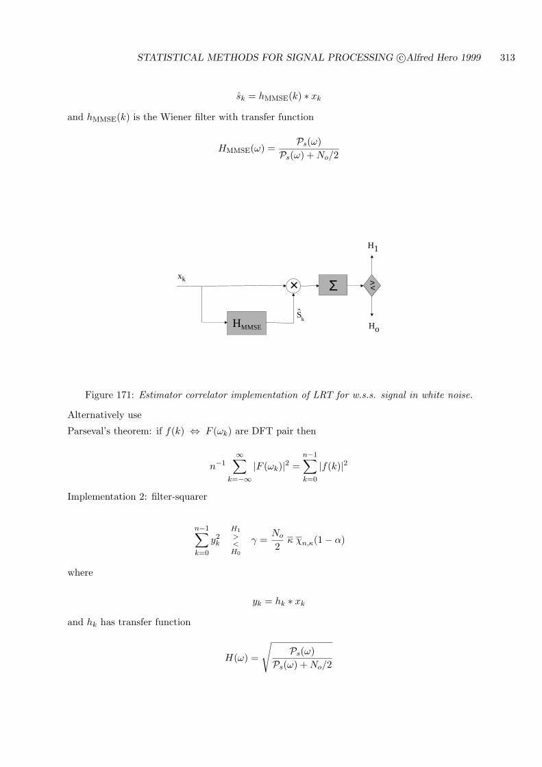
STATISTICAL METHODS FOR SIGNAL PROCESSING c©Alfred Hero 1999 313
sk = hMMSE(k) ∗ xk
and hMMSE(k) is the Wiener filter with transfer function
HMMSE(ω) =Ps(ω)
Ps(ω) + No/2
Ho
H1
> < xk Σ×
kS
HMMSE
Figure 171: Estimator correlator implementation of LRT for w.s.s. signal in white noise.
Alternatively use
Parseval’s theorem: if f(k) ⇔ F (ωk) are DFT pair then
n−1∞∑
k=−∞|F (ωk)|2 =
n−1∑
k=0
|f(k)|2
Implementation 2: filter-squarer
n−1∑
k=0
y2k
H1
><H0
γ =No
2κ χn,κ(1− α)
where
yk = hk ∗ xk
and hk has transfer function
H(ω) =
√Ps(ω)
Ps(ω) + No/2
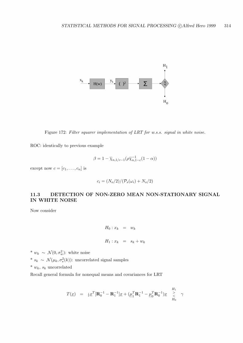
STATISTICAL METHODS FOR SIGNAL PROCESSING c©Alfred Hero 1999 314
Ho
H1
> < xk Σ( )2H(w)
yk
Figure 172: Filter squarer implementation of LRT for w.s.s. signal in white noise.
ROC: identically to previous example
β = 1− χn,1/c−1(ρχ−1n,1−c(1− α))
except now c = [c1, . . . , cn] is
ci = (No/2)/(Ps(ωi) + No/2)
11.3 DETECTION OF NON-ZERO MEAN NON-STATIONARY SIGNALIN WHITE NOISE
Now consider
H0 : xk = wk
H1 : xk = sk + wk
* wk ∼ N (0, σ2w): white noise
* sk ∼ N (µk, σ2s(k)): uncorrelated signal samples
* wk, sk uncorrelated
Recall general formula for nonequal means and covariances for LRT
T (x) = 12x
T [R−10 −R−1
1 ]x + (µT1R−1
1 − µT0R−1
0 )xH1
><H0
γ
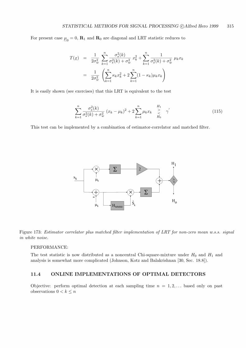
STATISTICAL METHODS FOR SIGNAL PROCESSING c©Alfred Hero 1999 315
For present case µ0
= 0, R1 and R0 are diagonal and LRT statistic reduces to
T (x) =1
2σ2w
n∑
k=1
σ2s(k)
σ2s(k) + σ2
w
x2k +
n∑
k=1
1σ2
s(k) + σ2w
µkxk
=1
2σ2w
(n∑
k=1
κkx2k + 2
n∑
k=1
(1− κk)µkxk
)
It is easily shown (see exercises) that this LRT is equivalent to the test
n∑
k=1
σ2s(k)
σ2s(k) + σ2
w
(xk − µk)2 + 2n∑
k=1
µkxk
H1
><H0
γ′
(115)
This test can be implemented by a combination of estimator-correlator and matched filter.
xk
Ho
H1
kS
HMMSE
+-
+
2
k
k
Figure 173: Estimator correlator plus matched filter implementation of LRT for non-zero mean w.s.s. signalin white noise.
PERFORMANCE:
The test statistic is now distributed as a noncentral Chi-square-mixture under H0 and H1 andanalysis is somewhat more complicated (Johnson, Kotz and Balakrishnan [30, Sec. 18.8]).
11.4 ONLINE IMPLEMENTATIONS OF OPTIMAL DETECTORS
Objective: perform optimal detection at each sampling time n = 1, 2, . . . based only on pastobservations 0 < k ≤ n
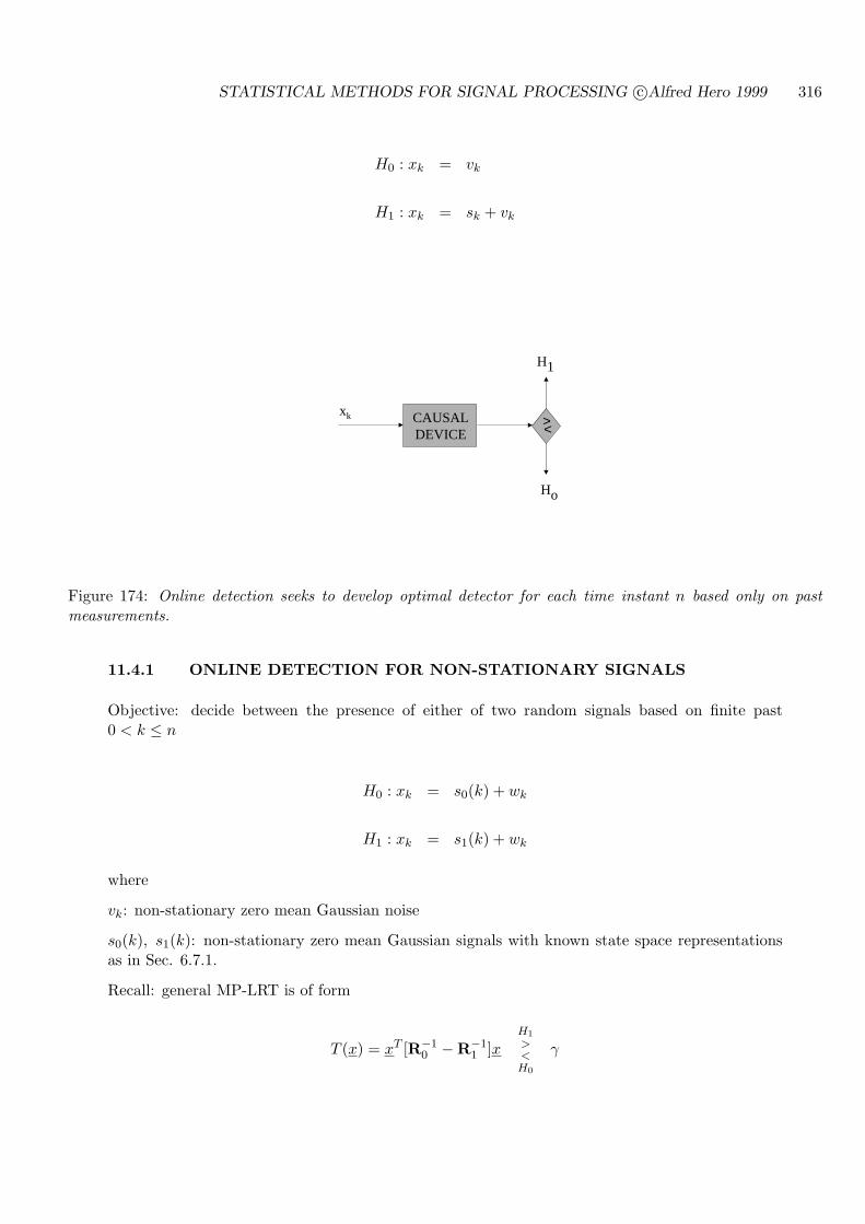
STATISTICAL METHODS FOR SIGNAL PROCESSING c©Alfred Hero 1999 316
H0 : xk = vk
H1 : xk = sk + vk
Ho
H1
> < CAUSALDEVICE
xk
Figure 174: Online detection seeks to develop optimal detector for each time instant n based only on pastmeasurements.
11.4.1 ONLINE DETECTION FOR NON-STATIONARY SIGNALS
Objective: decide between the presence of either of two random signals based on finite past0 < k ≤ n
H0 : xk = s0(k) + wk
H1 : xk = s1(k) + wk
where
vk: non-stationary zero mean Gaussian noise
s0(k), s1(k): non-stationary zero mean Gaussian signals with known state space representationsas in Sec. 6.7.1.
Recall: general MP-LRT is of form
T (x) = xT [R−10 −R−1
1 ]xH1
><H0
γ
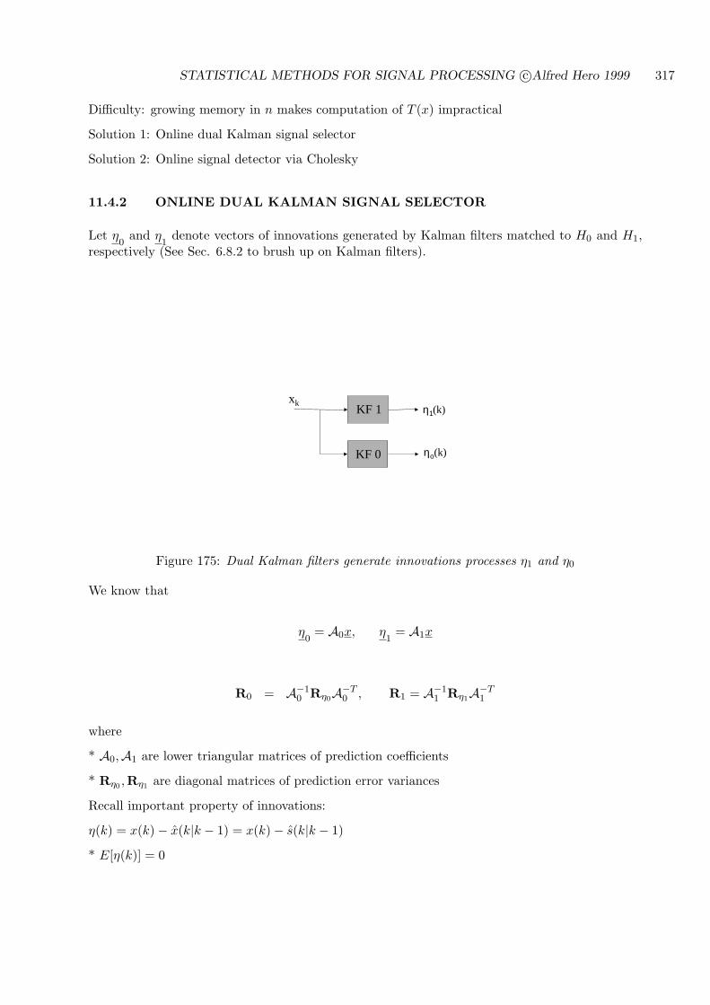
STATISTICAL METHODS FOR SIGNAL PROCESSING c©Alfred Hero 1999 317
Difficulty: growing memory in n makes computation of T (x) impractical
Solution 1: Online dual Kalman signal selector
Solution 2: Online signal detector via Cholesky
11.4.2 ONLINE DUAL KALMAN SIGNAL SELECTOR
Let η0
and η1
denote vectors of innovations generated by Kalman filters matched to H0 and H1,respectively (See Sec. 6.8.2 to brush up on Kalman filters).
xk
KF 1
η1(k)
ηο(k)KF 0
KF 1
Figure 175: Dual Kalman filters generate innovations processes η1 and η0
We know that
η0
= A0x, η1
= A1x
R0 = A−10 Rη0A−T
0 , R1 = A−11 Rη1A−T
1
where
* A0,A1 are lower triangular matrices of prediction coefficients
* Rη0 ,Rη1 are diagonal matrices of prediction error variances
Recall important property of innovations:
η(k) = x(k)− x(k|k − 1) = x(k)− s(k|k − 1)
* E[η(k)] = 0
STATISTICAL METHODS FOR SIGNAL PROCESSING c©Alfred Hero 1999 318
* var(η(k)) = cTRξ(k, k − 1)c︸ ︷︷ ︸
σ2s(k)
+σ2v is minimum prediction error variance
*
η(k)√var(η(k))
is white
* [η1, . . . , ηn]T ∼ Nn(0, diag(var(η(k)))I)
Using innovations representation we can re-express LR statistic
T (x) = xT [R−10 −R−1
1 ]x
= xT [ AT0 R−1
η0A0 − AT
1 R−1η1A1 ]x
= [A0x]T R−1η0
[A0x]︸ ︷︷ ︸η0
− [A1x]T R−1η1
[A1x]︸ ︷︷ ︸η1
Or, LRT reduces to
T (x) =n∑
i=1
η20(i)
var(η0(i))−
n∑
i=1
η21(i)
var(η1(i))
H1
><H0
γ
where, level α threshold is time varying. For example if R−10 > R−1
1
γ = n(1− c) χ−1n,1−c(1− α)
Special Case: SIGNAL DETECTION IN WHITE NOISE
Here s0(k) is zero and vk is white
H0 : xk = vk
H1 : xk = s1(k) + vk
and
* s0(k|k − 1) = 0
* η0(k) = xk
* var0(η0(k)) = σ2v
Thus MP-LRT simplifies to a “measured energy” vs. “Kalman residual” detector
T (x) =1σ2
v
n∑
i=1
x2i −
n∑
i=1
η21(i)
var(η1(i))
H1
><H0
γ
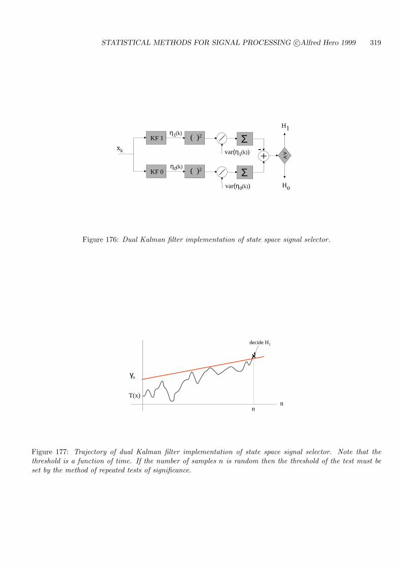
STATISTICAL METHODS FOR SIGNAL PROCESSING c©Alfred Hero 1999 319
xk
KF 1
+var(η1(k))
( )2 Σ
Ho
H1
> <
KF 0 ( )2 Σvar(η0(k))
η1(k)
η0(k)
-
Figure 176: Dual Kalman filter implementation of state space signal selector.
T(x)
γn
decide H1
nn
××××
Figure 177: Trajectory of dual Kalman filter implementation of state space signal selector. Note that thethreshold is a function of time. If the number of samples n is random then the threshold of the test must beset by the method of repeated tests of significance.
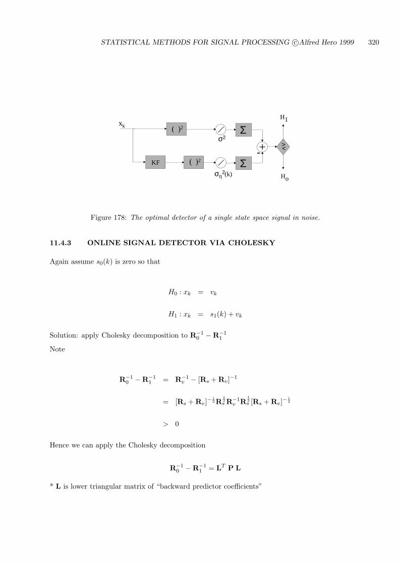
STATISTICAL METHODS FOR SIGNAL PROCESSING c©Alfred Hero 1999 320
+σ2
( )2 Σ
Ho
H1
> <
KF ( )2 Σση
2(k)
-
xk
Figure 178: The optimal detector of a single state space signal in noise.
11.4.3 ONLINE SIGNAL DETECTOR VIA CHOLESKY
Again assume s0(k) is zero so that
H0 : xk = vk
H1 : xk = s1(k) + vk
Solution: apply Cholesky decomposition to R−10 −R−1
1
Note
R−10 −R−1
1 = R−1v − [Rs + Rv]−1
= [Rs + Rv]−12 R
12s R−1
v R12s [Rs + Rv]−
12
> 0
Hence we can apply the Cholesky decomposition
R−10 −R−1
1 = LT P L
* L is lower triangular matrix of “backward predictor coefficients”
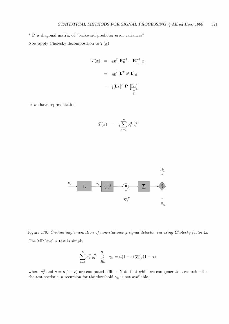
STATISTICAL METHODS FOR SIGNAL PROCESSING c©Alfred Hero 1999 321
* P is diagonal matrix of “backward predictor error variances”
Now apply Cholesky decomposition to T (x)
T (x) = 12x
T [R−10 −R−1
1 ]x
= 12x
T [LT P L]x
= 12 [Lx]T P [Lx]︸︷︷︸
y
or we have representation
T (x) = 12
n∑
i=1
σ2i y2
i
Ho
H1
> < xk Σ( )2L
yk ×
σk2
Figure 179: On-line implementation of non-stationary signal detector via using Cholesky factor L.
The MP level α test is simply
n∑
i=1
σ2i y2
i
H1
><H0
γn = n(1− c) χ−1n,κ(1− α)
where σ2i and κ = n(1− c) are computed offline. Note that while we can generate a recursion for
the test statistic, a recursion for the threshold γn is not available.
STATISTICAL METHODS FOR SIGNAL PROCESSING c©Alfred Hero 1999 322
In many cases yi can be generated by a “lumped” Kalman filter matched to a state observationmodel
x′k = s
′k + v
′k
s′k = cT
k νk
νk+1 = Dkνk + Ekw′k
synthesized such that the measurement covariance satisfies
Rx′ = R−10 −R−1
1
11.5 STEADY-STATE STATE-SPACE SIGNAL DETECTOR
Assume:
* State model for s1 is LTI
* measurement noise vk is w.s.s.
* limiting state error covariance matrix Rξ(∞) is non-singular
* Kalman filter is in steady state (n large)
Then, as innovations are w.s.s., the MP-LRT statistic can be written
T (x) =1
2σ2
n∑
i=1
x2i −
12var(η1)
n∑
i=1
η21(i)
H1
><H0
γ
Or, using asymptotic innovations variance, we have MP test
n∑
i=1
x2i −
σ2v
σ2s + σ2
v
n∑
i=1
η21(i)
H1
><H0
γ
APPROXIMATE GLRT FOR UNKNOWN MEASUREMENT NOISE VARIANCE
We can implement an approximate GLRT to handle the case where the variance of the observationnoise σ2
v is unknown. For this case the GLR statistic is
ΛGLR =
maxσ2v>0 (σ2
s + σ2v)−n/2 exp
(− 1
2(σ2s+σ2
v)
∑ni=1 η2
1(i))
maxσ2v>0 (σ2
v)−n/2 exp(− 1
2σ2v
∑ni=1 x2
i
)
Of course the denominator is maximized for
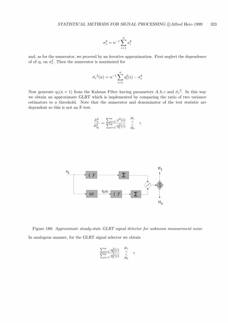
STATISTICAL METHODS FOR SIGNAL PROCESSING c©Alfred Hero 1999 323
σ2v = n−1
n∑
i=1
x2i
and, as for the numerator, we proceed by an iterative approximation. First neglect the dependenceof of η1 on σ2
v . Then the numerator is maximized for
σv2(n) = n−1
n∑
i=1
η21(i)− σ2
s
Now generate η1(n + 1) from the Kalman Filter having parameters A, b, c and σv2. In this way
we obtain an approximate GLRT which is implemented by comparing the ratio of two varianceestimators to a threshold. Note that the numerator and denominator of the test statistic aredependent so this is not an F-test.
σ2v
σ2η1
=∑n
i=1 x2(i)∑ni=1 η2
1(i)
H1
><H0
γ
( )2 Σ
Ho
H1
> <
KF ( )2 Σηi(k)
xk
Figure 180: Approximate steady-state GLRT signal detector for unknown measurement noise
In analogous manner, for the GLRT signal selector we obtain
∑ni=1 η2
0(i)∑ni=1 η2
1(i)
H1
><H0
γ
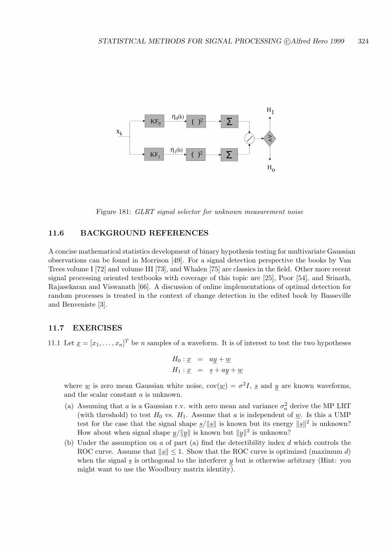
STATISTICAL METHODS FOR SIGNAL PROCESSING c©Alfred Hero 1999 324
Ho
H1
> <
KF1 ( )2 Ση1(k)
xk
KF0 ( )2 Ση0(k)
Figure 181: GLRT signal selector for unknown measurement noise
11.6 BACKGROUND REFERENCES
A concise mathematical statistics development of binary hypothesis testing for multivariate Gaussianobservations can be found in Morrison [49]. For a signal detection perspective the books by VanTrees volume I [72] and volume III [73], and Whalen [75] are classics in the field. Other more recentsignal processing oriented textbooks with coverage of this topic are [25], Poor [54], and Srinath,Rajasekaran and Viswanath [66]. A discussion of online implementations of optimal detection forrandom processes is treated in the context of change detection in the edited book by Bassevilleand Benveniste [3].
11.7 EXERCISES
11.1 Let x = [x1, . . . , xn]T be n samples of a waveform. It is of interest to test the two hypotheses
H0 : x = ay + w
H1 : x = s + ay + w
where w is zero mean Gaussian white noise, cov(w) = σ2I, s and y are known waveforms,and the scalar constant a is unknown.
(a) Assuming that a is a Gaussian r.v. with zero mean and variance σ2a derive the MP LRT
(with threshold) to test H0 vs. H1. Assume that a is independent of w. Is this a UMPtest for the case that the signal shape s/‖s‖ is known but its energy ‖s‖2 is unknown?How about when signal shape y/‖y‖ is known but ‖y‖2 is unknown?
(b) Under the assumption on a of part (a) find the detectibility index d which controls theROC curve. Assume that ‖s‖ ≤ 1. Show that the ROC curve is optimized (maximum d)when the signal s is orthogonal to the interferer y but is otherwise arbitrary (Hint: youmight want to use the Woodbury matrix identity).
STATISTICAL METHODS FOR SIGNAL PROCESSING c©Alfred Hero 1999 325
(c) Assuming that a is a deterministic unknown constant, repeat parts (a) and (b) for theGLRT of H0 vs. H1.
11.2 Let xk, k = 1, . . . , n be a segment of a discrete time random process. It is desired to testwhether xk contains a harmonic component (sinusoidal signal) or not
H0 : xk = wk
H1 : xk = A cos(ωok + ψ) + wk
where wk is zero mean Gaussian white noise with acf rw(k) = N0/2δk, ωo = 2πl/n for someinteger l, A is a deterministic amplitude, and ψ is a uniform phase over [0, 2π]. The randomphase of the sinusoid and the noise samples are independent of each other.
(a) Show that under H1 the auto-correlation function of xk is E[xixi−k] = rx(k) = A2/2 cos(ωok)+N0/2δk and derive the PSD Px.
(b) Derive the MP LRT with threshold and implement the MP LRT as an estimator correlatorand a filter squarer. (Hint: as ψ is uniform and f1(x|ψ) is a Gaussian p.d.f. f1(x) =(2π)−1
∫ 2π0 f1(x|ψ)dψ is a Bessel function of the form B0(r) = 1
2π
∫ π−π er cos ψdψ which is
monotone in a test statistic which under H0 is distributed as a Chi-square with 2 df, i.eexponential.)
(c) Show that the MP LRT can also be implemented as a test on the periodogram spectral es-timator Pper(ωo) = 1
n |DFTxkω=ωo |2 where DFTxkω =∑n
k=1 xke−jωk is the DTFT
of xknk=1, ω ∈ 2πl/nn
l=1.
11.3 Find the GLRT for the previous problem under the assumption that both A and ωo areunknown (Hint: as no closed form solution exists for the MLE’s of A and ωo you can leaveyour answer in the form of a “peak detector” block diagram).
11.4 Derive the “completion of the square” result (Eq. (115) in section 11.3.
11.5 A sensor is placed on a North Atlantic oil derick at a particular spatial location to monitorthe mechanical state of the structure. When the mechanical state is “normal” the sensorproduces a measurement which follows the state space model:
xk = sk + vk
sk+1 = ask + wk
k = 0, 1, . . .. A model for impending failure of the mechanical structure is that a shiftin the damping constant a occurs. Assuming the standard Gaussian assumptions on thedynamical model under both normal and failure modes, the detection of impending failurecan be formulated as testing between
H0 : a = ao
H1 : a 6= ao
where ao ∈ (−1, 1) is known.
(a) Implement the MP test of level α for the simple alternative H1 : a = a1, where a1 6= a0,with a pair of Kalman filters. If you solved Exercise 6.14 give explicit forms for yourfilters using the results of that exercise.
(b) Now treat the general composite case above with your favorite method, e.g. LMP orGLRT. Take this problem as far as you can by making simplifying assumptions startingwith assuming steady state operation of the Kalman filters.
STATISTICAL METHODS FOR SIGNAL PROCESSING c©Alfred Hero 1999 326
11.6 Available for observation are n time samples X(k),
X(k) =p∑
i=1
αigi(k − τi) + W (k), k = 1, . . . , n
where W (k) is a zero mean Gaussian white noise with variance var(W (k)) = σ2w, αi, i =
1, . . . , p, are p i.i.d. zero mean Gaussian random variables with variance σ2a, and gi(u),
i = 1, . . . , p, are p known time functions over u ∈ (−∞,∞). The αi and W (k) are uncorrelatedand p is known. Define K as the p× p matrix of inner products of the gi’s, i.e. K has entriesκij =
∑nk=1 gi(k − τi)gj(k − τj).
(a) Show that the ML estimator of the τi’s involves maximizing a quadratic form yT [I +ρK]−1y−b where y = [y1, . . . , yp]T is a vector of p correlator outputs yi(τi) =
∑nk=1 x(k)gi(k−
τi), i = 1, . . . , p, b = b(τ) is an observation independent bias term, and ρ = σ2a/σ2
w isthe SNR (Hint: express log-likelihood function in vector-matrix form and use a matrixinverse (Woodbury) identity). Draw a block diagram of your ML estimator implementedas a peak picker, i.e. a variable filter applied to the data over which you seek to maximizethe output.
(b) Now consider the detection problem
H0 : X(k) = W (k)
H1 : X(k) =p∑
i=1
αigi(k − τi) + W (k)
For known τi’s derive the LRT and draw a block diagrom of the detector. Is the LRTUMP for unknown τi’s? How about for known τi’s but unknown SNR σ2
a/σ2w?
(c) Now assume that the τi’s are unknown and that the αi’s are also unknown and non-random. Show that in the GLRT the maximization over the αi’s can be performedexplicitly. Draw a block diagram of the GLRT implemented with a thresholded peakpicker over the τi’s.
1. Observed is a random process xini=1 consisting of Gaussian random variables. Assume that
xk = sk + wk
where sk and wk are uncorrelated Gaussian variables with variances σ2s(k) and σ2
w, re-spectively. The noise wk is white and sk is uncorrelated over time but non-stationary,i.e., it has time varying variance. In this problem we assume that the instantaneous SNRγ(k) = σ2
s(k)/σ2w is known for all time but that the noise power level σ2
w is unknown.(a) For known σ2
w and zero mean wk and sk derive the MP test of the hypotheses (no needto set the threshold)
H0 : xk = wk
k = 1, . . . , n
H1 : xk = sk + wk
Does there exist a UMP test for unknown σ2w? If so what is it?
(b) Find the GLRT for the above hypotheses for unknown σ2w (no need to set the threshold).
(c) Now assume that sk has non-zero but constant mean µ = E[sk]. Find the GLRT forunknown µ and σ2
w (no need to set the threshold).
End of chapter
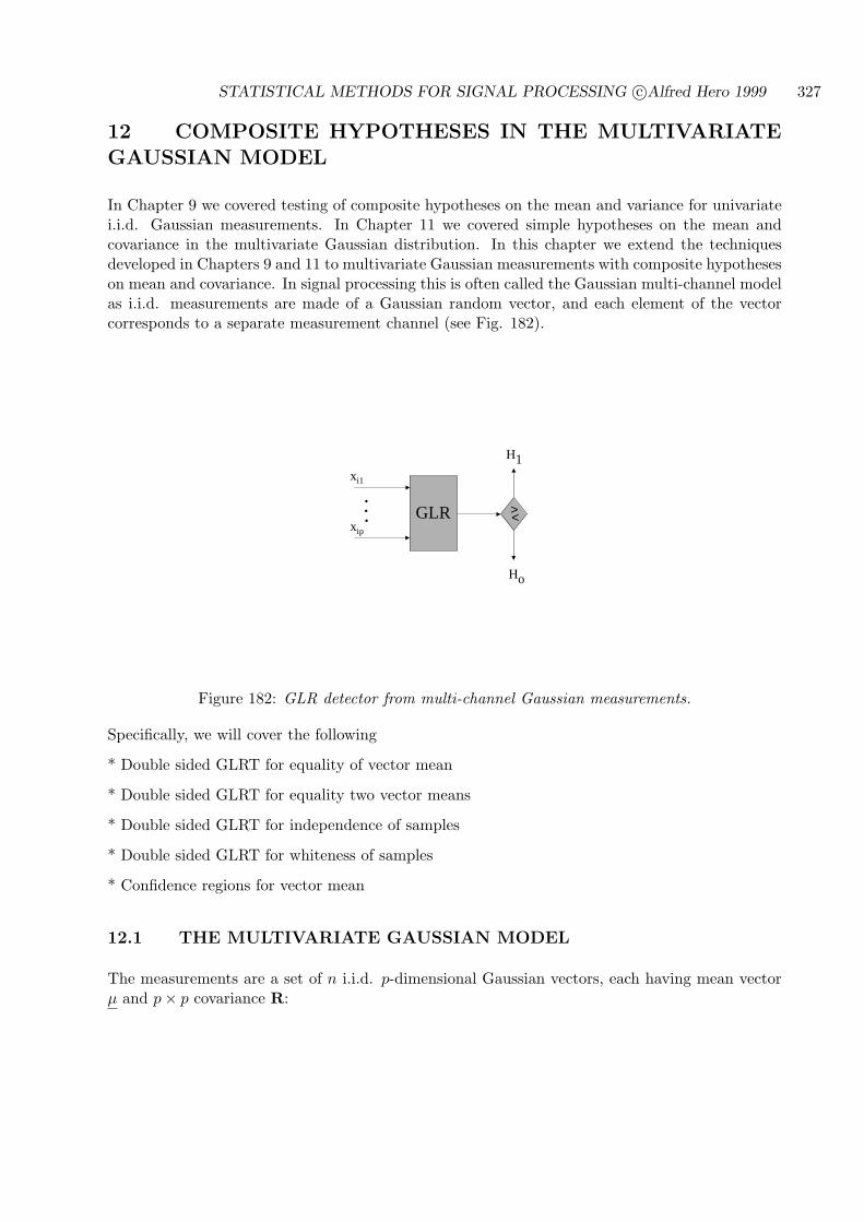
STATISTICAL METHODS FOR SIGNAL PROCESSING c©Alfred Hero 1999 327
12 COMPOSITE HYPOTHESES IN THE MULTIVARIATEGAUSSIAN MODEL
In Chapter 9 we covered testing of composite hypotheses on the mean and variance for univariatei.i.d. Gaussian measurements. In Chapter 11 we covered simple hypotheses on the mean andcovariance in the multivariate Gaussian distribution. In this chapter we extend the techniquesdeveloped in Chapters 9 and 11 to multivariate Gaussian measurements with composite hypotheseson mean and covariance. In signal processing this is often called the Gaussian multi-channel modelas i.i.d. measurements are made of a Gaussian random vector, and each element of the vectorcorresponds to a separate measurement channel (see Fig. 182).
Ho
> <GLR
H1xi1
xip• • •
Figure 182: GLR detector from multi-channel Gaussian measurements.
Specifically, we will cover the following
* Double sided GLRT for equality of vector mean
* Double sided GLRT for equality two vector means
* Double sided GLRT for independence of samples
* Double sided GLRT for whiteness of samples
* Confidence regions for vector mean
12.1 THE MULTIVARIATE GAUSSIAN MODEL
The measurements are a set of n i.i.d. p-dimensional Gaussian vectors, each having mean vectorµ and p× p covariance R:
STATISTICAL METHODS FOR SIGNAL PROCESSING c©Alfred Hero 1999 328
Xi =
Xi1...
Xip
, i = 1, . . . n
For notational convenience we denote the measurements by a random p× n measurement matrix
X = [X1, . . . , Xn]
This matrix has the following properties:
* Xini=1: independent Gaussian columns (n ≥ p)
* µ = Eθ[Xi]: mean vector
* R = covθ(Xi): covariance matrix (p× p)
The jpdf of the Gaussian matrix X has the form
f(X; µ,R)
=(
1(2π)p |R|
)n/2
exp
(−1
2
n∑
i=1
(Xi − µ)TR−1(Xi − µ)
)
=(
1(2π)p |R|
)n/2
exp
(−1
2
n∑
i=1
trace(Xi − µ)(Xi − µ)TR−1
)
=(
1(2π)p |R|
)n/2
exp(−n
2traceRµ R
)
where we have defined the p× p covariance estimator
Rµ = n−1n∑
i=1
(Xi − µ)(Xi − µ)T
=1n
(X− µ1T )(X− µ1T )T
12.2 DOUBLE SIDED TEST OF VECTOR MEAN
We pose the two hypotheses:
H0 : µ = µo, R > 0 (116)
H1 : µ 6= µo, R > 0. (117)
the GLRT of these hypotheses is
ΛGLR =maxµ,R>0 f(X; µ,R)
maxR>0 f(X; µo,R)
.
STATISTICAL METHODS FOR SIGNAL PROCESSING c©Alfred Hero 1999 329
Now, it is easily seen that
maxµ,R>0
f(X;µ,R) = maxR>0
f(X; X,R)
where the column sample mean is defined as
X = n−1n∑
i=1
Xi = X11n
.
Therefore, we can rewrite the GLRT as
ΛGLR =maxµ,R>0 f(X; µ,R)
maxR>0 f(X;µo,R)
=maxR>0 |R|−n/2 exp
(−1
2 traceRXR−1
)
maxR>0 |R|−n/2 exp(−n
2 traceRµR−1
)
FACT: for any vector t = [t1, . . . , p]T
maxR>0
|R|−n/2 exp
(−n
2trace
RtR−1
)= |Rt|−n/2 e−n2/2
and the maximum is attained by
R = Rt = n−1n∑
i=1
(Xi − t)(Xi − t)T
Proof:
The maximizing R also maximizes
l(R) = ln f(X; t,R) =n
2ln |R| − n
2trace
RtR−1
Define the transformed covariance R
R = R−1/2t R R−1/2
t .
Then, since the trace and the determinant satisfy
traceAB = traceBA, |AB| = |BA| = |B| |A|,we have
l(R) = −n
2
(ln |R1/2
t RR1/2t | + trace
R1/2
t R−1R−1/2t
)
= −n
2
(ln |RtR| + trace
R−1
)
= −n
2
(ln |Rt|+ ln |R| + trace
R−1
)
= −n
2
ln |Rt|+
p∑
j=1
ln λj +p∑
j=1
1λj
STATISTICAL METHODS FOR SIGNAL PROCESSING c©Alfred Hero 1999 330
where λj are the eigenvalues of R
Hence the maximizing R satisfies for j = 1, . . . , p
0 =d
dλj
l(R)
= −n
2
(1λj
− 1λ2
j
)
so that the maximizing R has identical eigenvalues
λj = 1, j = 1, . . . , p.
This implies that the maximizing R is an orthogonal (unitary) matrix U. But, since R is alsosymmetric, R is in fact the p× p identityo
ThereforeI = R = R−1/2
t RR−1/2t
giving the maximizing R asR = Rt,
as claimed. ¦Note: We have just shown that
1. The MLE of R for known µ = µo
is
Rµ = n−1n∑
i=1
(Xi − µo)(Xi − µ
o)T .
2. The MLE of R for unknown µ is
RX = R = n−1n∑
i=1
(Xi −X)(Xi −X)T .
Plugging the above MLE solutions back into GLRT statistic for testing (117)
ΛGLR =
( |Rµo|
|R|
)n/2
=(∣∣∣Rµ
oR−1
∣∣∣)n/2
.
UsingRµ
o= R + (X − µ
o)(X − µ
o)T ,
0If U is orthogonal then UH = U−1 matrix I. If in addition U is symmetric then U = UT = U−1 so that U = I.
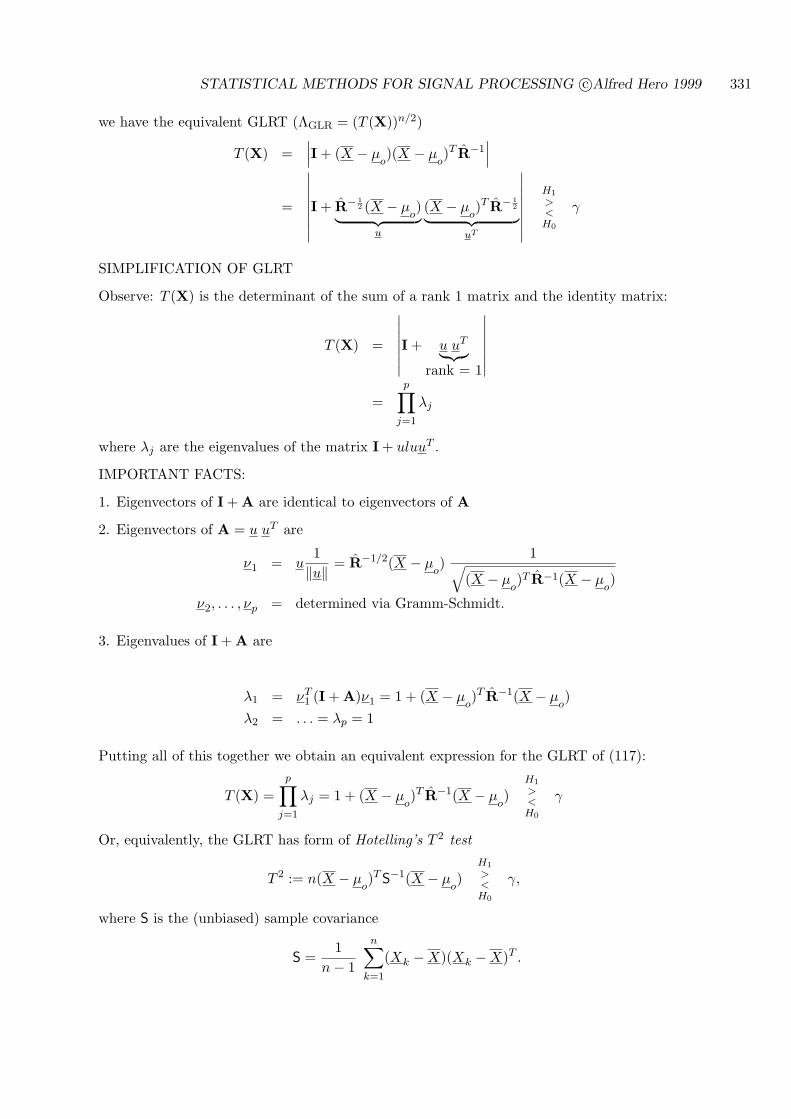
STATISTICAL METHODS FOR SIGNAL PROCESSING c©Alfred Hero 1999 331
we have the equivalent GLRT (ΛGLR = (T (X))n/2)
T (X) =∣∣∣I + (X − µ
o)(X − µ
o)T R−1
∣∣∣
=
∣∣∣∣∣∣∣∣I + R− 1
2 (X − µo)︸ ︷︷ ︸
u
(X − µo)T R− 1
2
︸ ︷︷ ︸uT
∣∣∣∣∣∣∣∣
H1
><H0
γ
SIMPLIFICATION OF GLRT
Observe: T (X) is the determinant of the sum of a rank 1 matrix and the identity matrix:
T (X) =
∣∣∣∣∣∣∣I + u uT
︸︷︷︸rank = 1
∣∣∣∣∣∣∣
=p∏
j=1
λj
where λj are the eigenvalues of the matrix I + uluuT .
IMPORTANT FACTS:
1. Eigenvectors of I + A are identical to eigenvectors of A
2. Eigenvectors of A = u uT are
ν1 = u1‖u‖ = R−1/2(X − µ
o)
1√(X − µ
o)T R−1(X − µ
o)
ν2, . . . , νp = determined via Gramm-Schmidt.
3. Eigenvalues of I + A are
λ1 = νT1 (I + A)ν1 = 1 + (X − µ
o)T R−1(X − µ
o)
λ2 = . . . = λp = 1
Putting all of this together we obtain an equivalent expression for the GLRT of (117):
T (X) =p∏
j=1
λj = 1 + (X − µo)T R−1(X − µ
o)
H1
><H0
γ
Or, equivalently, the GLRT has form of Hotelling’s T 2 test
T 2 := n(X − µo)T S−1(X − µ
o)
H1
><H0
γ,
where S is the (unbiased) sample covariance
S =1
n− 1
n∑
k=1
(Xk −X)(Xk −X)T .
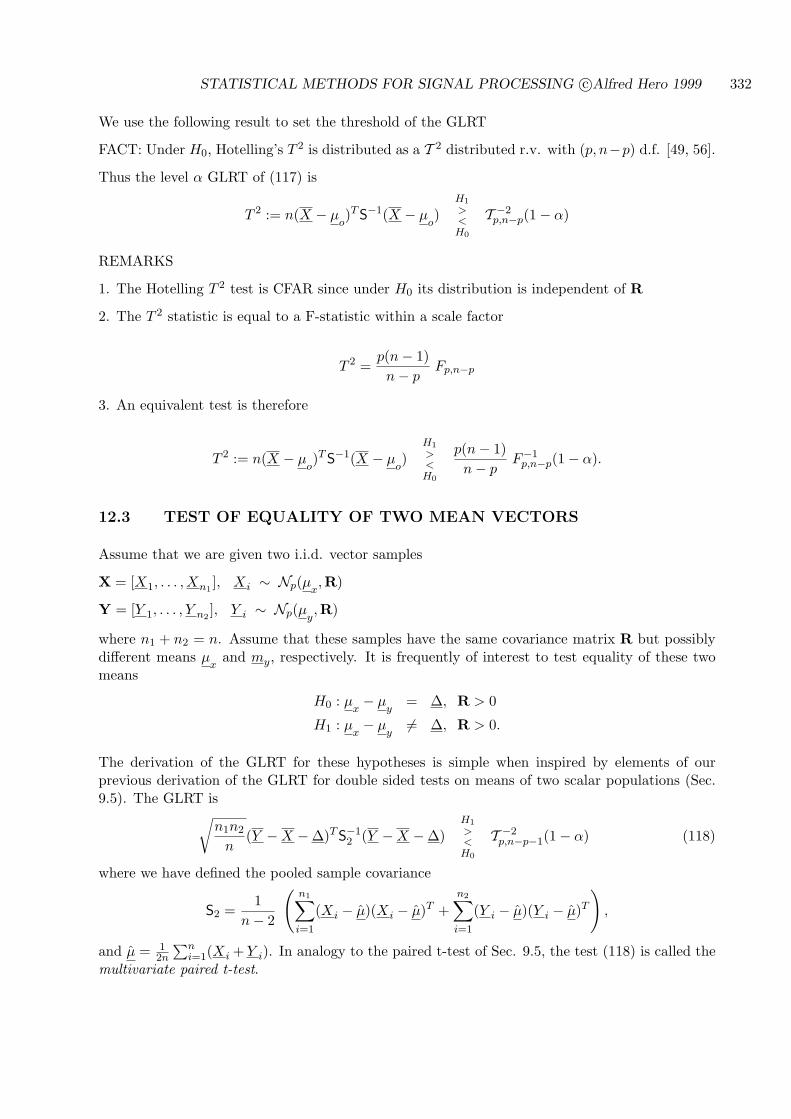
STATISTICAL METHODS FOR SIGNAL PROCESSING c©Alfred Hero 1999 332
We use the following result to set the threshold of the GLRT
FACT: Under H0, Hotelling’s T 2 is distributed as a T 2 distributed r.v. with (p, n−p) d.f. [49, 56].
Thus the level α GLRT of (117) is
T 2 := n(X − µo)T S−1(X − µ
o)
H1
><H0
T −2p,n−p(1− α)
REMARKS
1. The Hotelling T 2 test is CFAR since under H0 its distribution is independent of R
2. The T 2 statistic is equal to a F-statistic within a scale factor
T 2 =p(n− 1)n− p
Fp,n−p
3. An equivalent test is therefore
T 2 := n(X − µo)T S−1(X − µ
o)
H1
><H0
p(n− 1)n− p
F−1p,n−p(1− α).
12.3 TEST OF EQUALITY OF TWO MEAN VECTORS
Assume that we are given two i.i.d. vector samples
X = [X1, . . . , Xn1], Xi ∼ Np(µx
,R)
Y = [Y 1, . . . , Y n2], Y i ∼ Np(µy
,R)
where n1 + n2 = n. Assume that these samples have the same covariance matrix R but possiblydifferent means µ
xand my, respectively. It is frequently of interest to test equality of these two
means
H0 : µx− µ
y= ∆, R > 0
H1 : µx− µ
y6= ∆, R > 0.
The derivation of the GLRT for these hypotheses is simple when inspired by elements of ourprevious derivation of the GLRT for double sided tests on means of two scalar populations (Sec.9.5). The GLRT is
√n1n2
n(Y −X −∆)T S−1
2 (Y −X −∆)H1
><H0
T −2p,n−p−1(1− α) (118)
where we have defined the pooled sample covariance
S2 =1
n− 2
(n1∑
i=1
(Xi − µ)(Xi − µ)T +n2∑
i=1
(Y i − µ)(Y i − µ)T
),
and µ = 12n
∑ni=1(Xi + Y i). In analogy to the paired t-test of Sec. 9.5, the test (118) is called the
multivariate paired t-test.

STATISTICAL METHODS FOR SIGNAL PROCESSING c©Alfred Hero 1999 333
12.4 TEST OF INDEPENDENCE
n i.i.d. vector samples
X = [X1, . . . , Xn], Xi ∼ Np(µ,R)
To test
H0 : R = diag(σ2j )
H1 : R 6= diag(σ2j )
with mean vector µ unknown
ΛGLR =maxR6=diag,µ f(X;µ,R)
maxR=diag,µ f(X;µ,R)=
maxR>0 |R|−n/2 exp(−1
2
∑nk=1(Xk −X)TR−1(Xk −X)
)
maxσ2j >0
(∏pk=1 σ2
k
)−n/2 exp(−1
2
∑nk=1
1σ2
k‖Xk −X)‖2
)
Using previous results
ΛGLR =
(∏pj=1 σ2
j
|R|
)n/2 H1
><H0
γ
where we have the variance estimate for each channel (row) of X
σ2j :=
1n
n∑
k=1
(Xk −X)2j
For n large we can set γ by using Chi-square asymptotics
2 ln ΛGLR
H1
><H0
γ′= χ−1
p(p−1)/2(1− α)
Calculation of degrees of freedom ν:
ν = # parameters fixed under H0
1. p2 − p = p(p− 1) off diagonals in R
2. 1/2 of these off diagonals are identical
⇒ ν = p(p− 1)/2
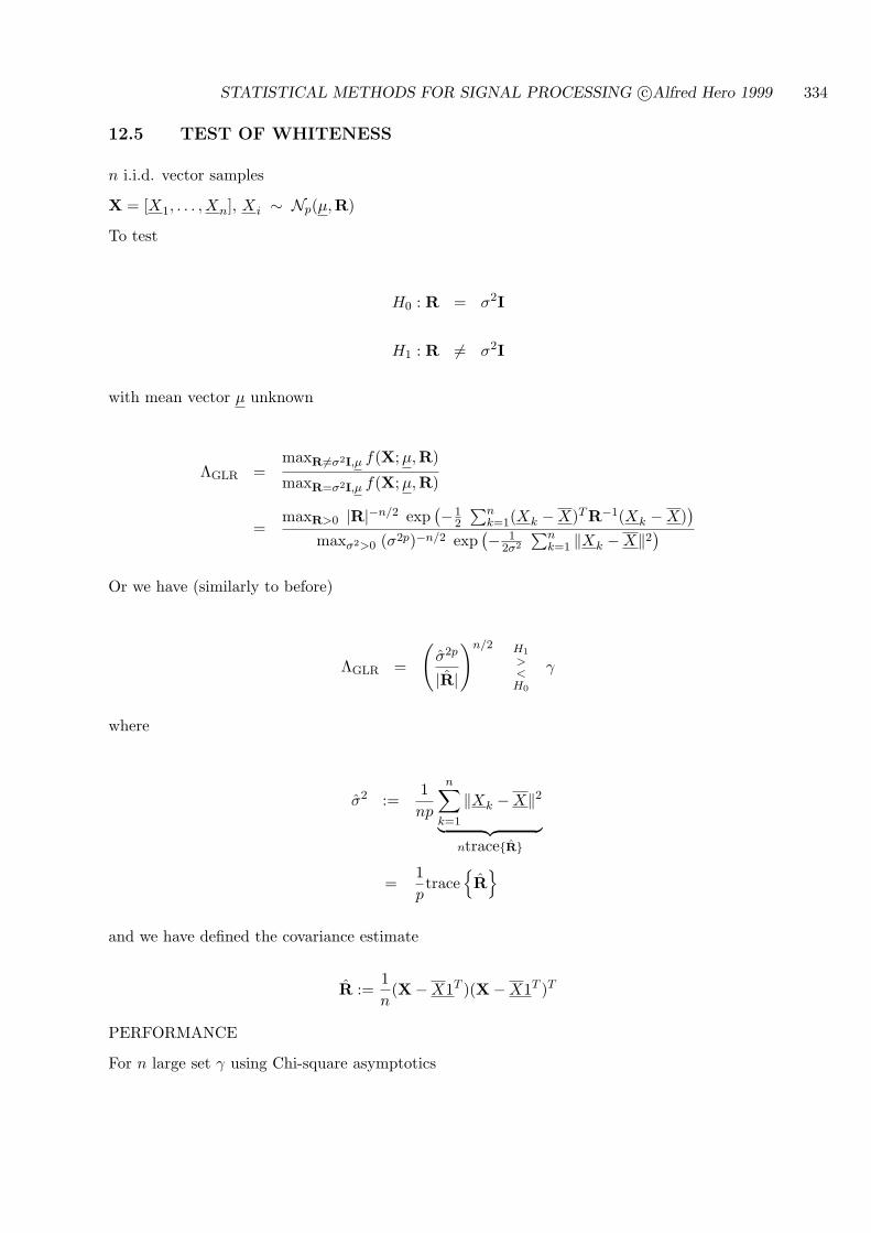
STATISTICAL METHODS FOR SIGNAL PROCESSING c©Alfred Hero 1999 334
12.5 TEST OF WHITENESS
n i.i.d. vector samples
X = [X1, . . . , Xn], Xi ∼ Np(µ,R)
To test
H0 : R = σ2I
H1 : R 6= σ2I
with mean vector µ unknown
ΛGLR =maxR6=σ2I,µ f(X; µ,R)
maxR=σ2I,µ f(X; µ,R)
=maxR>0 |R|−n/2 exp
(−12
∑nk=1(Xk −X)TR−1(Xk −X)
)
maxσ2>0 (σ2p)−n/2 exp(− 1
2σ2
∑nk=1 ‖Xk −X‖2
)
Or we have (similarly to before)
ΛGLR =
(σ2p
|R|
)n/2 H1
><H0
γ
where
σ2 :=1np
n∑
k=1
‖Xk −X‖2
︸ ︷︷ ︸ntraceR
=1ptrace
R
and we have defined the covariance estimate
R :=1n
(X−X1T )(X−X1T )T
PERFORMANCE
For n large set γ using Chi-square asymptotics
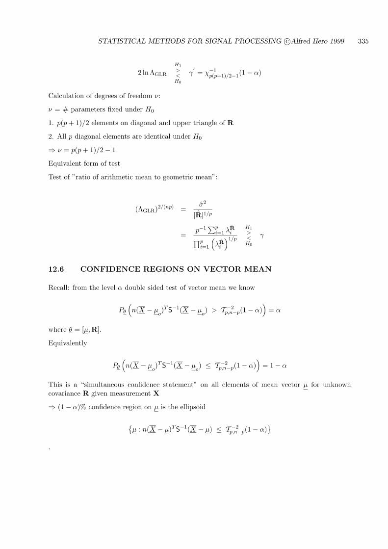
STATISTICAL METHODS FOR SIGNAL PROCESSING c©Alfred Hero 1999 335
2 ln ΛGLR
H1
><H0
γ′= χ−1
p(p+1)/2−1(1− α)
Calculation of degrees of freedom ν:
ν = # parameters fixed under H0
1. p(p + 1)/2 elements on diagonal and upper triangle of R
2. All p diagonal elements are identical under H0
⇒ ν = p(p + 1)/2− 1
Equivalent form of test
Test of ”ratio of arithmetic mean to geometric mean”:
(ΛGLR)2/(np) =σ2
|R|1/p
=p−1
∑pi=1 λR
i
∏pi=1
(λR
i
)1/p
H1
><H0
γ
12.6 CONFIDENCE REGIONS ON VECTOR MEAN
Recall: from the level α double sided test of vector mean we know
Pθ
(n(X − µ
o)T S−1(X − µ
o) > T −2
p,n−p(1− α))
= α
where θ = [µ,R].
Equivalently
Pθ
(n(X − µ
o)T S−1(X − µ
o) ≤ T −2
p,n−p(1− α))
= 1− α
This is a “simultaneous confidence statement” on all elements of mean vector µ for unknowncovariance R given measurement X
⇒ (1− α)% confidence region on µ is the ellipsoid
µ : n(X − µ)T S−1(X − µ) ≤ T −2
p,n−p(1− α)
.

STATISTICAL METHODS FOR SIGNAL PROCESSING c©Alfred Hero 1999 336
x
(1-α)% confidence region
µ1
µ2
Figure 183: Confidence region for all elements of mean vector µ is an ellipsoid
µ1
µ2
x .
Figure 184: Confidence ellipsoid gives “marginal” confidence intervals on each element of µ = [µ1, . . . , µp]T
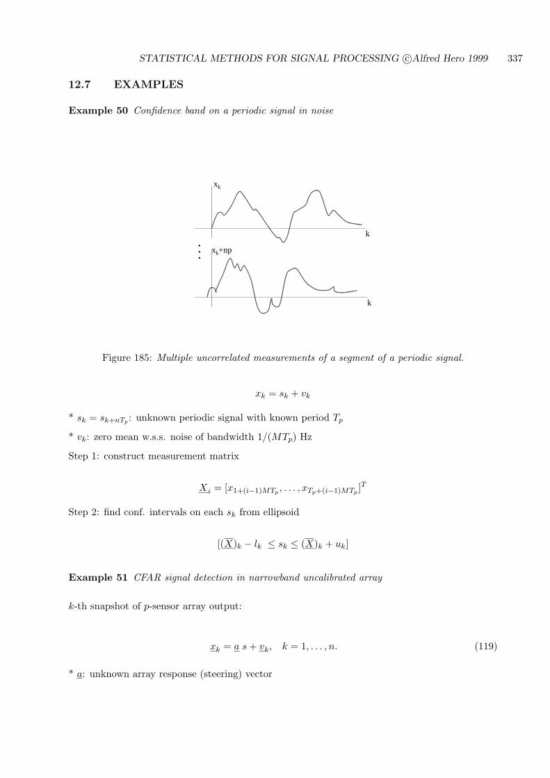
STATISTICAL METHODS FOR SIGNAL PROCESSING c©Alfred Hero 1999 337
12.7 EXAMPLES
Example 50 Confidence band on a periodic signal in noise
k
k
xk+np...
xk
Figure 185: Multiple uncorrelated measurements of a segment of a periodic signal.
xk = sk + vk
* sk = sk+nTp : unknown periodic signal with known period Tp
* vk: zero mean w.s.s. noise of bandwidth 1/(MTp) Hz
Step 1: construct measurement matrix
Xi = [x1+(i−1)MTp, . . . , xTp+(i−1)MTp
]T
Step 2: find conf. intervals on each sk from ellipsoid
[(X)k − lk ≤ sk ≤ (X)k + uk]
Example 51 CFAR signal detection in narrowband uncalibrated array
k-th snapshot of p-sensor array output:
xk = a s + vk, k = 1, . . . , n. (119)
* a: unknown array response (steering) vector

STATISTICAL METHODS FOR SIGNAL PROCESSING c©Alfred Hero 1999 338
k
xk
Figure 186: Confidence band on signal over one signal period.
Figure 187: Sensor array generates spatio-temporal measurement.
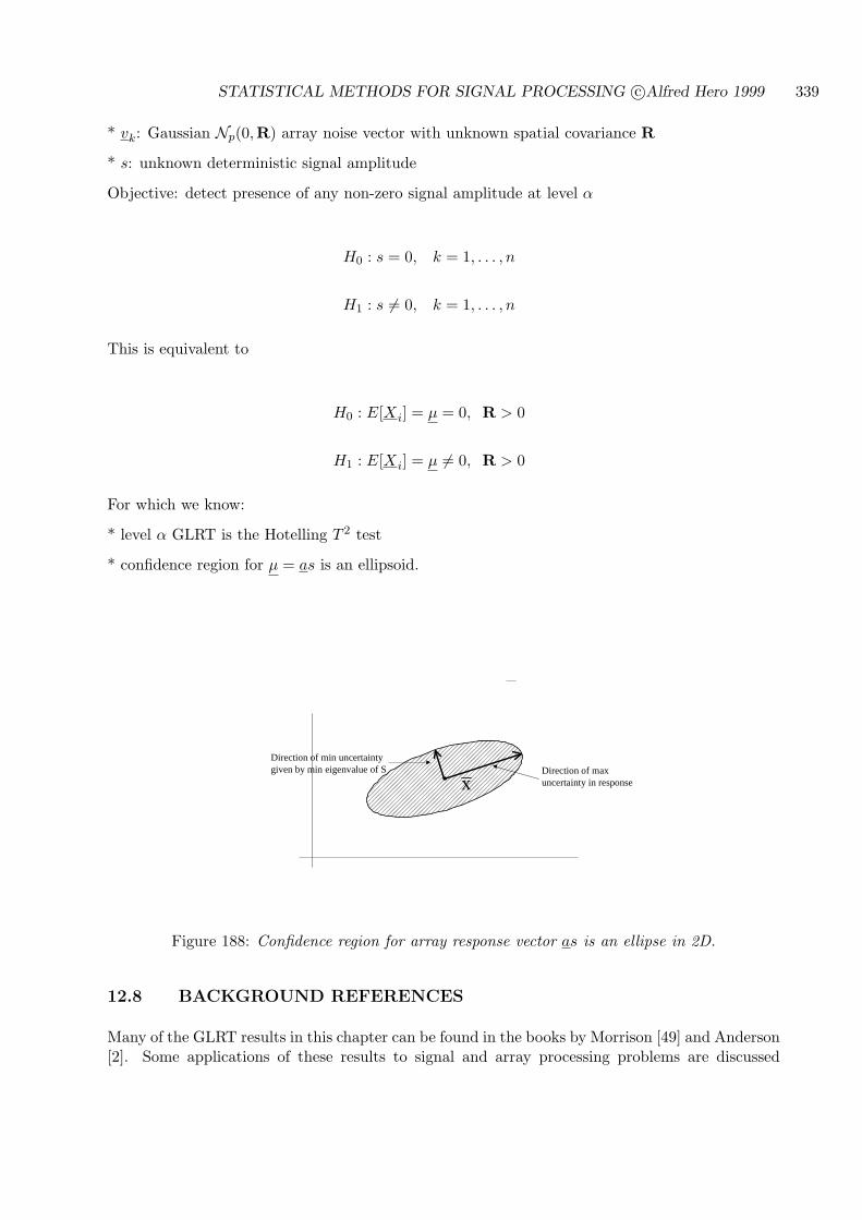
STATISTICAL METHODS FOR SIGNAL PROCESSING c©Alfred Hero 1999 339
* vk: Gaussian Np(0,R) array noise vector with unknown spatial covariance R
* s: unknown deterministic signal amplitude
Objective: detect presence of any non-zero signal amplitude at level α
H0 : s = 0, k = 1, . . . , n
H1 : s 6= 0, k = 1, . . . , n
This is equivalent to
H0 : E[Xi] = µ = 0, R > 0
H1 : E[Xi] = µ 6= 0, R > 0
For which we know:
* level α GLRT is the Hotelling T 2 test
* confidence region for µ = as is an ellipsoid.
xDirection of max uncertainty in response
Direction of min uncertaintygiven by min eigenvalue of S
Figure 188: Confidence region for array response vector as is an ellipse in 2D.
12.8 BACKGROUND REFERENCES
Many of the GLRT results in this chapter can be found in the books by Morrison [49] and Anderson[2]. Some applications of these results to signal and array processing problems are discussed

STATISTICAL METHODS FOR SIGNAL PROCESSING c©Alfred Hero 1999 340
in Van Trees [72]. More applications of detection theory to multi-channel problems arising inarray processing and spectral estimation can be found in Haykin [24] and Stoica and Moses [68].The books by Eaton [15], Mardia, Kent and Bibby [43], and Muirhead [50] give more advancedtreatments of general multivariate analysis techniques and testing of composite hypotheses. Theproblem of constructing confidence regions for vector parameter is closely related to the problemof simultaneous confidence intervals and this topic is covered in detail by Miller [46]. Miller’s bookdoes not cover the popular and more flexible False Discovery Rate (FDR) as an alternative toconfidence level, for which the reader is referred to Benjamini and Yekutieli’s paper [5] and itshypothesis testing homolog by Benjamini and Hochberg [4].
12.9 EXERCISES
12.1 Extend the multivariate paired-t test derived in Sec. 12.3 to the case where xi ∼ N (µx, Rx)
and yi∼ N (µ
y, Ry) for the case that the two covariance matrices Rx and Ry may be un-
equal and are unknown. How many degrees of freedom does the the asymptotic Chi-squaredistribution have?
12.2 In Example 51 the optimal CFAR detector for a scalar signal s viewed from a p-sensor arrayoutput with array response a and noise vk. In this problem we extend this to CFAR detectionof multiple (m) scalar signals s = [s1, . . . , sm] following the observation model:
xk = As + vk, k = 1, . . . , n (120)
where A = [a1, . . . , ap] is an unknown p×m matrix and vk are i.i.d. N (0, R) random vectorswith unknown covariance R. Derive the GLRT for this problem. How many degrees offreedom does the the asymptotic Chi-square distribution have?
12.3 Consider the same model as (119) but assume that s is a Gaussian distributed random variableand a and R are unknown. Derive the GLRT.
12.4 Consider the same scalar model as (119) but now assume that a is known while the noisecovariance R is unknown. Derive the GLRT.
12.5 Extend the analysis of the previous problem to the multiple signal case (120) when A hascolumns of sinusoidal form:
ak = [1, cos(2πfk), . . . , cos(2πfk(p− 1))]T , k = 1, . . . , m
while the noise covariance R is unknown. Derive the GLRT (you may assume that the ak’sare orthogonal if you wish).
End of chapter
STATISTICAL METHODS FOR SIGNAL PROCESSING c©Alfred Hero 1999 341
13 BIBLIOGRAPHY
References
[1] M. Abromowitz and I. Stegun, Handbook of Mathematical Functions, Dover, New York, N.Y.,1965.
[2] T. W. Anderson, An Introduction to Multivariate Statistical Analysis, Wiley, New York, 1958.
[3] M. Basseville and A. Benveniste, editors, Detection of abrupt changes in signals and dynamicalsystems, Springer Lecture Notes in Control and Information Sciences, 1986.
[4] Y. Benjamini and Y. Hochberg, “Controlling the false discovery rate: A practical and powerfulapproach to multiple testing,” J. Royal Statistical Society, vol. 57, pp. 289–300, 1995.
[5] Y. Benjamini and D. Yekutieli, “False discovery rate adjusted confidence intervals for selectedparameters (preprint),” J. Am. Statist. Assoc., vol. 100, no. 469, pp. 71–81, March 2005.
[6] R. Beran, “Pivoting to reduce level error of confidence sets,” Biometrika, vol. 74, pp. 457–468,1987.
[7] P. J. Bickel and K. A. Doksum, Mathematical Statistics: Basic Ideas and Selected Topics,Holden-Day, San Francisco, 1977.
[8] H. Bode and C. Shannon, “A simplified derivation of linear least squares smoothing andprediction theory,” Proc. of the Institute of Radio Engineers (IRE), vol. 38, pp. 417–425,April 1950.
[9] S. Bose and A. O. Steinhardt, “Adaptive array detection of uncertain rank one waveforms,”Signal Processing, vol. 44, no. 11, pp. 2801–2809, Nov. 1996.
[10] S. Bose and A. O. Steinhardt, “A maximal invariant framework for adaptive detection withstructured and unstructured covariance matrices,” Signal Processing, vol. 43, no. 9, pp. 2164–2175, Sept. 1995.
[11] D. R. Brillinger, Time Series: Data Analysis and Theory, Springer-Verlag, New York, 1981.
[12] P. J. Brockwell and R. A. Davis, Time Series: Theory and Methods, Springer-Verlag, NewYork, 1987.
[13] W. Davenport and W. Root, An introduction to the theory of random signals and noise, IEEEPress, New York (reprint of 1958 McGraw-Hill edition), 1987.
[14] M. DeGroot, Optimal Statistical decisions, McGraw Hill, NJ, 1970.
[15] M. L. Eaton, Multivariate Statistics - A Vector Space Approach, Wiley, New York, 1983.
[16] T. S. Ferguson, Mathematical Statistics - A Decision Theoretic Approach, Academic Press,Orlando FL, 1967.
[17] A. Gelman, J. B. Carlin, H. S. Stern, and D. B. Rubin, Bayesian Data Analysis, Chapmanand Hall/CRC, Boca Raton, 1995.
[18] M. Gevers and T. Kailath, “An innovations approach to least squares estimation, part vi:Discrete-time innovations representations and recursive estimation,” IEEE Trans. AutomaticControl, vol. AC-18, pp. 588–600, Dec. 1973.
[19] G. H. Golub and C. F. Van Loan, Matrix Computations (2nd Edition), The Johns HopkinsUniversity Press, Baltimore, 1989.
STATISTICAL METHODS FOR SIGNAL PROCESSING c©Alfred Hero 1999 342
[20] J. D. Gorman and A. O. Hero, “Lower bounds for parametric estimation with constraints,”IEEE Trans. on Inform. Theory, vol. IT-36, pp. 1285–1301, Nov. 1990.
[21] F. A. Graybill, Matrices with Applications in Statistics, Wadsworth Publishing Co., BelmontCA, 1983.
[22] G. Hardy, J. Littlewood, and G. Polya, Inequalities (2nd Edition), Cambridge Univ. Press,1951.
[23] M. H. Hayes, Statistical Digital Signal Processing and Modeling, Wiley, New York, 1996.
[24] S. Haykin, Array Signal Processing, Prentice-Hall, Englewood Cliffs NJ, 1985.
[25] C. Helstrom, Elements of signal detection and estimation, Prentice-Hall, Englewood Cliffs,1995.
[26] J. U. Hjorth, Computer intensive statistical methods, CHapman and Hall, London, 1994.
[27] D. C. Hoaglin, F. Mosteller, and J. W. Tukey, Understanding robust and exploratory dataanalysis, Wiley, New York, 1983.
[28] M. Hollander and D. A. Wolfe, Nonparametric statistical methods (2nd Edition), Wiley, NewYork, 1991.
[29] I. A. Ibragimov and R. Z. Has’minskii, Statistical estimation: Asymptotic theory, Springer-Verlag, New York, 1981.
[30] N. L. Johnson, S. Kotz, and A. W. N. Balakrishnan, Continuous univariate distributions:Vol. 1, Wiley, New York, 1994.
[31] N. L. Johnson, S. Kotz, and A. W. N. Balakrishnan, Continuous univariate distributions:Vol. 2, Wiley, New York, 1995.
[32] T. Kailath, Lectures on Wiener and Kalman Filtering, Springer-Verlag, New York, 1981.
[33] T. Kariya and B. K. Sinha, Robustness of Statistical Tests, Academic Press, San Diego, 1989.
[34] R. Kass and P. Vos, Geometrical Foundations of Asymptotic Inference, Wiley, New York,1997.
[35] S. Kassam and J. Thomas, Nonparametric detection - theory and applications, Dowden,Hutchinson and Ross, 1980.
[36] S. M. Kay, Statistical Estimation, Prentice-Hall, Englewood-Cliffs N.J., 1991.
[37] G. F. Knoll, Radiation Detection, Wiley, New York, 1985.
[38] E. L. Lehmann, Testing Statistical Hypotheses, Wiley, New York, 1959.
[39] E. L. Lehmann, Theory of Point Estimation, Wiley, New York, 1983.
[40] E. L. Lehmann, Theory of Point Estimation, 2nd Edition, Wiley, New York, 1991.
[41] D. G. Luenberger, Optimization by Vector Space Methods, Wiley, New York, 1969.
[42] E. B. Manoukian, Modern Concepts and Theorems of Mathematical Statistics, Springer-Verlag, New York N.Y., 1986.
[43] K. V. Mardia, J. T. Kent, and J. M. Bibby, Multivariate Analysis, Academic Press, NewYork, 1979.
[44] J. M. Mendel, Lessons in estimation for signal processing, communications, and control,Prentice-Hall, Englewood Cliffs NJ, 1995.
[45] D. Middleton, “Statistical methods for the detection of pulsed radar in noise,” in Communi-cation Theory, W. Jackson, editor, pp. 241–270, Academic Press, New York, 1953.
STATISTICAL METHODS FOR SIGNAL PROCESSING c©Alfred Hero 1999 343
[46] R. G. Miller, Simultaneous Statistical Inference, Springer-Verlag, NY, 1981.
[47] A. M. Mood, F. A. Graybill, and D. C. Boes, Introduction to the Theory of Statistics, McGrawHill, New York, 1976.
[48] T. K. Moon and W. C. Stirling, Mathematical methods and algorithms for signal processing,Prentice Hall, Englewood Cliffs, 2000.
[49] D. F. Morrison, Multivariate statistical methods, McGraw Hill, New York, 1967.
[50] R. J. Muirhead, Aspects of Multivariate Statistical Theory, Wiley, New York, 1982.
[51] B. Noble and J. W. Daniel, Applied Linear Algebra, Prentice Hall, Englewood Cliffs, NJ, 1977.
[52] A. V. Oppenheim and A. S. Willsky, Signals and Systems, Prentice-Hall, Englewood Cliffs,N.J., 1983.
[53] A. Papoulis, Probability, random variables, and stochastic processes (3rd ed), McGraw Hill,New York, N.Y., 1991.
[54] H. V. Poor, An Introduction to Signal Detection and Estimation, Springer-Verlag, New York,1988.
[55] J. G. Proakis and D. G. Manolakis, Digital signal processing: principles, algorithms, andapplications, Prentice-Hall, NY, 1996.
[56] C. R. Rao, Linear Statistical Inference and Its Applications, Wiley, New York, 1973.
[57] J. P. Romano and A. F. Siegel, Counterexamples in probability and statistics, Wadsworth,Belmont CA, 1983.
[58] S. Ross, A first course in probability, Prentice-Hall, Englewood Cliffs, N.J., 1998.
[59] L. L. Scharf, Statistical Signal Processing: Detection, Estimation, and Time Series Analysis,Addison-Wesley, Reading, MA, 1991.
[60] L. L. Scharf and D. W. Lytle, “Signal detection in Gaussian noise of unknown level: aninvariance application,” IEEE Trans. on Inform. Theory, vol. IT-17, no. 3, pp. 404–411,1971.
[61] R. J. Serfling, Approximation Theorems of Mathematical Statistics, Wiley, New York, 1980.
[62] M. Shao and C. Nikias, “Signal processing with fractional lower order moments: Stableprocesses and their applications,” Proceedings of the IEEE, vol. 81, no. 7, pp. 986–1010, July1993.
[63] G. E. Shilov, Linear Algebra, Dover Publications, New York, N.Y., 1977.
[64] D. L. Snyder and M. I. Miller, Random Point Processes in Time and Space, Springer-Verlag,New York, 1991.
[65] T. Soderstrom and P. Stoica, System identification, Prentice Hall, Englewood Cliffs NJ, 1989.
[66] M. D. Srinath, P. K. Rajasekaran, and R. Viswanathan, Introduction to statistical signalprocessing with applications, Prentice Hall, Englewood Cliffs, 1996.
[67] H. Stark and J. Woods, Probability, Random Processes, and Estimation Theory for Engineers,Prentice-Hall, Englewood Cliffs, N.J., 1986.
[68] P. Stoica and R. Moses, Introduction to spectral analysis, Prentice-Hall, Englewood Cliffs NJ,1997.
[69] P. Strobach, Linear Prediction Theory: A Mathematical Basis for Adaptive Systems, Springer-Verlag, New York, 1990.

STATISTICAL METHODS FOR SIGNAL PROCESSING c©Alfred Hero 1999 344
[70] M. A. Tanner, Tools for Statistical Inference; Methods for the exploration of posterior distri-butions and likelihood functions, Springer-Verlag, New York, 1993.
[71] J. B. Thomas, An Introduction to Statistical Communications Theory, Wiley, New York, 1969.
[72] H. L. Van-Trees, Detection, Estimation, and Modulation Theory: Part I, Wiley, New York,1968.
[73] H. L. Van-Trees, Detection, Estimation, and Modulation Theory: Part III, Wiley, New York,2001.
[74] R. E. Walpole, R. H. Myers, and S. L. Myers, Probability and statistics for engineers andscientists, Prentice Hall, New Jersey, 1998.
[75] A. D. Whalen, Detection of Signals in Noise (2nd Ed.), Academic Press, Orlando, 1995.


![[Monson H. Hayes] Statistical Digital Signal Processing](https://img.pdfslide.net/doc/110x75/563db7e3550346aa9a8ee680/monson-h-hayes-statistical-digital-signal-processing.jpg)