Statistical Science2001, Vol. 16, No. 3, 199–231

Statistical Modeling: The Two CulturesLeo Breiman

Abstract. There are two cultures in the use of statistical modeling toreach conclusions from data. One assumes that the data are generatedby a given stochastic data model. The other uses algorithmic models andtreats the data mechanism as unknown. The statistical community hasbeen committed to the almost exclusive use of data models. This commit-ment has led to irrelevant theory, questionable conclusions, and has keptstatisticians from working on a large range of interesting current prob-lems. Algorithmic modeling, both in theory and practice, has developedrapidly in fields outside statistics. It can be used both on large complexdata sets and as a more accurate and informative alternative to datamodeling on smaller data sets. If our goal as a field is to use data tosolve problems, then we need to move away from exclusive dependenceon data models and adopt a more diverse set of tools.

1. INTRODUCTION

Statistics starts with data. Think of the data asbeing generated by a black box in which a vector ofinput variables x (independent variables) go in oneside, and on the other side the response variables ycome out. Inside the black box, nature functions toassociate the predictor variables with the responsevariables, so the picture is like this:

y xnature

There are two goals in analyzing the data:

Prediction. To be able to predict what the responsesare going to be to future input variables;Information. To extract some information abouthow nature is associating the response variablesto the input variables.

There are two different approaches toward thesegoals:

The Data Modeling Culture

The analysis in this culture starts with assuminga stochastic data model for the inside of the blackbox. For example, a common data model is that dataare generated by independent draws from

response variables = f(predictor variables,random noise, parameters)

Leo Breiman is Professor, Department of Statistics,University of California, Berkeley, California 94720-4735 (e-mail: leo@stat.berkeley.edu).

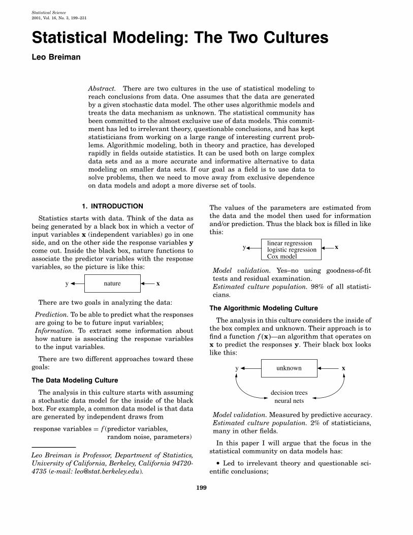
The values of the parameters are estimated fromthe data and the model then used for informationand/or prediction. Thus the black box is filled in likethis:

y xlinear regression logistic regressionCox model

Model validation. Yes–no using goodness-of-fittests and residual examination.Estimated culture population. 98% of all statisti-cians.

The Algorithmic Modeling Culture

The analysis in this culture considers the inside ofthe box complex and unknown. Their approach is tofind a function f�x�—an algorithm that operates onx to predict the responses y. Their black box lookslike this:

y xunknown

decision treesneural nets

Model validation.Measured by predictive accuracy.Estimated culture population. 2% of statisticians,many in other fields.

In this paper I will argue that the focus in thestatistical community on data models has:

• Led to irrelevant theory and questionable sci-entific conclusions;

199

200 L. BREIMAN

• Kept statisticians from using more suitablealgorithmic models;• Prevented statisticians from working on excit-

ing new problems;

I will also review some of the interesting newdevelopments in algorithmic modeling in machinelearning and look at applications to three data sets.

2. ROAD MAP

It may be revealing to understand how I became amember of the small second culture. After a seven-year stint as an academic probabilist, I resigned andwent into full-time free-lance consulting. After thir-teen years of consulting I joined the Berkeley Statis-tics Department in 1980 and have been there since.My experiences as a consultant formed my viewsabout algorithmic modeling. Section 3 describes twoof the projects I worked on. These are given to showhow my views grew from such problems.When I returned to the university and began

reading statistical journals, the research was dis-tant from what I had done as a consultant. Allarticles begin and end with data models. My obser-vations about published theoretical research instatistics are in Section 4.Data modeling has given the statistics field many

successes in analyzing data and getting informa-tion about the mechanisms producing the data. Butthere is also misuse leading to questionable con-clusions about the underlying mechanism. This isreviewed in Section 5. Following that is a discussion(Section 6) of how the commitment to data modelinghas prevented statisticians from entering new sci-entific and commercial fields where the data beinggathered is not suitable for analysis by data models.In the past fifteen years, the growth in algorith-

mic modeling applications and methodology hasbeen rapid. It has occurred largely outside statis-tics in a new community—often called machinelearning—that is mostly young computer scientists(Section 7). The advances, particularly over the lastfive years, have been startling. Three of the mostimportant changes in perception to be learned fromthese advances are described in Sections 8, 9, and10, and are associated with the following names:

Rashomon: the multiplicity of good models;Occam: the conflict between simplicity andaccuracy;Bellman: dimensionality—curse or blessing?

Section 11 is titled “Information from a BlackBox” and is important in showing that an algo-rithmic model can produce more and more reliableinformation about the structure of the relationship

between inputs and outputs than data models. Thisis illustrated using two medical data sets and agenetic data set. A glossary at the end of the paperexplains terms that not all statisticians may befamiliar with.

3. PROJECTS IN CONSULTING

As a consultant I designed and helped supervisesurveys for the Environmental Protection Agency(EPA) and the state and federal court systems. Con-trolled experiments were designed for the EPA, andI analyzed traffic data for the U.S. Department ofTransportation and the California TransportationDepartment. Most of all, I worked on a diverse setof prediction projects. Here are some examples:

Predicting next-day ozone levels.Using mass spectra to identify halogen-containingcompounds.Predicting the class of a ship from high altituderadar returns.Using sonar returns to predict the class of a sub-marine.Identity of hand-sent Morse Code.Toxicity of chemicals.On-line prediction of the cause of a freeway trafficbreakdown.Speech recognitionThe sources of delay in criminal trials in state courtsystems.

To understand the nature of these problems andthe approaches taken to solve them, I give a fullerdescription of the first two on the list.

3.1 The Ozone Project

In the mid- to late 1960s ozone levels became aserious health problem in the Los Angeles Basin.Three different alert levels were established. At thehighest, all government workers were directed notto drive to work, children were kept off playgroundsand outdoor exercise was discouraged.The major source of ozone at that time was auto-

mobile tailpipe emissions. These rose into the lowatmosphere and were trapped there by an inversionlayer. A complex chemical reaction, aided by sun-light, cooked away and produced ozone two to threehours after the morning commute hours. The alertwarnings were issued in the morning, but would bemore effective if they could be issued 12 hours inadvance. In the mid-1970s, the EPA funded a largeeffort to see if ozone levels could be accurately pre-dicted 12 hours in advance.Commuting patterns in the Los Angeles Basin

are regular, with the total variation in any given

STATISTICAL MODELING: THE TWO CULTURES 201

daylight hour varying only a few percent fromone weekday to another. With the total amount ofemissions about constant, the resulting ozone lev-els depend on the meteorology of the precedingdays. A large data base was assembled consist-ing of lower and upper air measurements at U.S.weather stations as far away as Oregon and Ari-zona, together with hourly readings of surfacetemperature, humidity, and wind speed at thedozens of air pollution stations in the Basin andnearby areas.Altogether, there were daily and hourly readings

of over 450 meteorological variables for a period ofseven years, with corresponding hourly values ofozone and other pollutants in the Basin. Let x bethe predictor vector of meteorological variables onthe nth day. There are more than 450 variables inx since information several days back is included.Let y be the ozone level on the �n + 1�st day. Thenthe problem was to construct a function f�x� suchthat for any future day and future predictor vari-ables x for that day, f�x� is an accurate predictor ofthe next day’s ozone level y.To estimate predictive accuracy, the first five

years of data were used as the training set. Thelast two years were set aside as a test set. Thealgorithmic modeling methods available in the pre-1980s decades seem primitive now. In this projectlarge linear regressions were run, followed by vari-able selection. Quadratic terms in, and interactionsamong, the retained variables were added and vari-able selection used again to prune the equations. Inthe end, the project was a failure—the false alarmrate of the final predictor was too high. I haveregrets that this project can’t be revisited with thetools available today.

3.2 The Chlorine Project

The EPA samples thousands of compounds a yearand tries to determine their potential toxicity. Inthe mid-1970s, the standard procedure was to mea-sure the mass spectra of the compound and to tryto determine its chemical structure from its massspectra.Measuring the mass spectra is fast and cheap. But

the determination of chemical structure from themass spectra requires a painstaking examinationby a trained chemist. The cost and availability ofenough chemists to analyze all of the mass spectraproduced daunted the EPA. Many toxic compoundscontain halogens. So the EPA funded a project todetermine if the presence of chlorine in a compoundcould be reliably predicted from its mass spectra.Mass spectra are produced by bombarding the

compound with ions in the presence of a magnetic

field. The molecules of the compound split and thelighter fragments are bent more by the magneticfield than the heavier. Then the fragments hit anabsorbing strip, with the position of the fragment onthe strip determined by the molecular weight of thefragment. The intensity of the exposure at that posi-tion measures the frequency of the fragment. Theresultant mass spectra has numbers reflecting fre-quencies of fragments from molecular weight 1 up tothe molecular weight of the original compound. Thepeaks correspond to frequent fragments and thereare many zeroes. The available data base consistedof the known chemical structure and mass spectraof 30,000 compounds.The mass spectrum predictor vector x is of vari-

able dimensionality. Molecular weight in the database varied from 30 to over 10,000. The variable tobe predicted is

y = 1: contains chlorine,

y = 2: does not contain chlorine.

The problem is to construct a function f�x� thatis an accurate predictor of y where x is the massspectrum of the compound.To measure predictive accuracy the data set was

randomly divided into a 25,000 member trainingset and a 5,000 member test set. Linear discrim-inant analysis was tried, then quadratic discrimi-nant analysis. These were difficult to adapt to thevariable dimensionality. By this time I was thinkingabout decision trees. The hallmarks of chlorine inmass spectra were researched. This domain knowl-edge was incorporated into the decision tree algo-rithm by the design of the set of 1,500 yes–no ques-tions that could be applied to a mass spectra of anydimensionality. The result was a decision tree thatgave 95% accuracy on both chlorines and nonchlo-rines (see Breiman, Friedman, Olshen and Stone,1984).

3.3 Perceptions on Statistical Analysis

As I left consulting to go back to the university,these were the perceptions I had about working withdata to find answers to problems:

(a) Focus on finding a good solution—that’s whatconsultants get paid for.

(b) Live with the data before you plunge intomodeling.

(c) Search for a model that gives a good solution,either algorithmic or data.

(d) Predictive accuracy on test sets is the crite-rion for how good the model is.

(e) Computers are an indispensable partner.

202 L. BREIMAN

4. RETURN TO THE UNIVERSITY

I had one tip about what research in the uni-versity was like. A friend of mine, a prominentstatistician from the Berkeley Statistics Depart-ment, visited me in Los Angeles in the late 1970s.After I described the decision tree method to him,his first question was, “What’s the model for thedata?”

4.1 Statistical Research

Upon my return, I started reading the Annals ofStatistics, the flagship journal of theoretical statis-tics, and was bemused. Every article started with

Assume that the data are generated by the follow-ing model: � � �

followed by mathematics exploring inference, hypo-thesis testing and asymptotics. There is a widespectrum of opinion regarding the usefulness of thetheory published in the Annals of Statistics to thefield of statistics as a science that deals with data. Iam at the very low end of the spectrum. Still, therehave been some gems that have combined nicetheory and significant applications. An example iswavelet theory. Even in applications, data modelsare universal. For instance, in the Journal of theAmerican Statistical Association �JASA�, virtuallyevery article contains a statement of the form:

Assume that the data are generated by the follow-ing model: � � �

I am deeply troubled by the current and past useof data models in applications, where quantitativeconclusions are drawn and perhaps policy decisionsmade.

5. THE USE OF DATA MODELS

Statisticians in applied research consider datamodeling as the template for statistical analysis:Faced with an applied problem, think of a datamodel. This enterprise has at its heart the beliefthat a statistician, by imagination and by lookingat the data, can invent a reasonably good para-metric class of models for a complex mechanismdevised by nature. Then parameters are estimatedand conclusions are drawn. But when a model is fitto data to draw quantitative conclusions:

• The conclusions are about the model’s mecha-nism, and not about nature’s mechanism.

It follows that:

• If the model is a poor emulation of nature, theconclusions may be wrong.

These truisms have often been ignored in the enthu-siasm for fitting data models. A few decades ago,the commitment to data models was such that evensimple precautions such as residual analysis orgoodness-of-fit tests were not used. The belief in theinfallibility of data models was almost religious. Itis a strange phenomenon—once a model is made,then it becomes truth and the conclusions from itare infallible.

5.1 An Example

I illustrate with a famous (also infamous) exam-ple: assume the data is generated by independentdraws from the model

�R� y = b0 +M∑1

bmxm + ε

where the coefficients �bm� are to be estimated, εis N�0 σ2� and σ2 is to be estimated. Given thatthe data is generated this way, elegant tests ofhypotheses, confidence intervals, distributions ofthe residual sum-of-squares and asymptotics can bederived. This made the model attractive in termsof the mathematics involved. This theory was usedboth by academic statisticians and others to derivesignificance levels for coefficients on the basis ofmodel (R), with little consideration as to whetherthe data on hand could have been generated by alinear model. Hundreds, perhaps thousands of arti-cles were published claiming proof of something orother because the coefficient was significant at the5% level.Goodness-of-fit was demonstrated mostly by giv-

ing the value of the multiple correlation coefficientR2 which was often closer to zero than one andwhich could be over inflated by the use of too manyparameters. Besides computing R2, nothing elsewas done to see if the observational data could havebeen generated by model (R). For instance, a studywas done several decades ago by a well-knownmember of a university statistics department toassess whether there was gender discrimination inthe salaries of the faculty. All personnel files wereexamined and a data base set up which consisted ofsalary as the response variable and 25 other vari-ables which characterized academic performance;that is, papers published, quality of journals pub-lished in, teaching record, evaluations, etc. Genderappears as a binary predictor variable.A linear regression was carried out on the data

and the gender coefficient was significant at the5% level. That this was strong evidence of sex dis-crimination was accepted as gospel. The designof the study raises issues that enter before theconsideration of a model—Can the data gathered

STATISTICAL MODELING: THE TWO CULTURES 203

answer the question posed? Is inference justifiedwhen your sample is the entire population? Shoulda data model be used? The deficiencies in analysisoccurred because the focus was on the model andnot on the problem.The linear regression model led to many erro-

neous conclusions that appeared in journal articleswaving the 5% significance level without knowingwhether the model fit the data. Nowadays, I thinkmost statisticians will agree that this is a suspectway to arrive at conclusions. At the time, there werefew objections from the statistical profession aboutthe fairy-tale aspect of the procedure, But, hidden inan elementary textbook, Mosteller and Tukey (1977)discuss many of the fallacies possible in regressionand write “The whole area of guided regression isfraught with intellectual, statistical, computational,and subject matter difficulties.”Even currently, there are only rare published cri-

tiques of the uncritical use of data models. One ofthe few is David Freedman, who examines the useof regression models (1994); the use of path models(1987) and data modeling (1991, 1995). The analysisin these papers is incisive.

5.2 Problems in Current Data Modeling

Current applied practice is to check the datamodel fit using goodness-of-fit tests and residualanalysis. At one point, some years ago, I set up asimulated regression problem in seven dimensionswith a controlled amount of nonlinearity. Standardtests of goodness-of-fit did not reject linearity untilthe nonlinearity was extreme. Recent theory sup-ports this conclusion. Work by Bickel, Ritov andStoker (2001) shows that goodness-of-fit tests havevery little power unless the direction of the alter-native is precisely specified. The implication is thatomnibus goodness-of-fit tests, which test in manydirections simultaneously, have little power, andwill not reject until the lack of fit is extreme.Furthermore, if the model is tinkered with on the

basis of the data, that is, if variables are deletedor nonlinear combinations of the variables added,then goodness-of-fit tests are not applicable. Resid-ual analysis is similarly unreliable. In a discussionafter a presentation of residual analysis in a sem-inar at Berkeley in 1993, William Cleveland, oneof the fathers of residual analysis, admitted that itcould not uncover lack of fit in more than four to fivedimensions. The papers I have read on using resid-ual analysis to check lack of fit are confined to datasets with two or three variables.With higher dimensions, the interactions between

the variables can produce passable residual plots for

a variety of models. A residual plot is a goodness-of-fit test, and lacks power in more than a few dimen-sions. An acceptable residual plot does not implythat the model is a good fit to the data.There are a variety of ways of analyzing residuals.

For instance, Landwher, Preibon and Shoemaker(1984, with discussion) gives a detailed analysis offitting a logistic model to a three-variable data setusing various residual plots. But each of the fourdiscussants present other methods for the analysis.One is left with an unsettled sense about the arbi-trariness of residual analysis.Misleading conclusions may follow from data

models that pass goodness-of-fit tests and residualchecks. But published applications to data oftenshow little care in checking model fit using thesemethods or any other. For instance, many of thecurrent application articles in JASA that fit datamodels have very little discussion of how well theirmodel fits the data. The question of how well themodel fits the data is of secondary importance com-pared to the construction of an ingenious stochasticmodel.

5.3 The Multiplicity of Data Models

One goal of statistics is to extract informationfrom the data about the underlying mechanism pro-ducing the data. The greatest plus of data modelingis that it produces a simple and understandable pic-ture of the relationship between the input variablesand responses. For instance, logistic regression inclassification is frequently used because it producesa linear combination of the variables with weightsthat give an indication of the variable importance.The end result is a simple picture of how the pre-diction variables affect the response variable plusconfidence intervals for the weights. Suppose twostatisticians, each one with a different approachto data modeling, fit a model to the same dataset. Assume also that each one applies standardgoodness-of-fit tests, looks at residuals, etc., andis convinced that their model fits the data. Yetthe two models give different pictures of nature’smechanism and lead to different conclusions.McCullah and Nelder (1989) write “Data will

often point with almost equal emphasis on sev-eral possible models, and it is important that thestatistician recognize and accept this.” Well said,but different models, all of them equally good, maygive different pictures of the relation between thepredictor and response variables. The question ofwhich one most accurately reflects the data is dif-ficult to resolve. One reason for this multiplicityis that goodness-of-fit tests and other methods forchecking fit give a yes–no answer. With the lack of

204 L. BREIMAN

power of these tests with data having more than asmall number of dimensions, there will be a largenumber of models whose fit is acceptable. There isno way, among the yes–no methods for gauging fit,of determining which is the better model. A fewstatisticians know this. Mountain and Hsiao (1989)write, “It is difficult to formulate a comprehensivemodel capable of encompassing all rival models.Furthermore, with the use of finite samples, thereare dubious implications with regard to the validityand power of various encompassing tests that relyon asymptotic theory.”Data models in current use may have more dam-

aging results than the publications in the social sci-ences based on a linear regression analysis. Just asthe 5% level of significance became a de facto stan-dard for publication, the Cox model for the analysisof survival times and logistic regression for survive–nonsurvive data have become the de facto standardfor publication in medical journals. That differentsurvival models, equally well fitting, could give dif-ferent conclusions is not an issue.

5.4 Predictive Accuracy

The most obvious way to see how well the modelbox emulates nature’s box is this: put a case x downnature’s box getting an output y. Similarly, put thesame case x down the model box getting an out-put y′. The closeness of y and y′ is a measure ofhow good the emulation is. For a data model, thistranslates as: fit the parameters in your model byusing the data, then, using the model, predict thedata and see how good the prediction is.Prediction is rarely perfect. There are usu-

ally many unmeasured variables whose effect isreferred to as “noise.” But the extent to which themodel box emulates nature’s box is a measure ofhow well our model can reproduce the naturalphenomenon producing the data.McCullagh and Nelder (1989) in their book on

generalized linear models also think the answer isobvious. They write, “At first sight it might seemas though a good model is one that fits the datavery well; that is, one that makes µ (the model pre-dicted value) very close to y (the response value).”Then they go on to note that the extent of the agree-ment is biased by the number of parameters usedin the model and so is not a satisfactory measure.They are, of course, right. If the model has too manyparameters, then it may overfit the data and give abiased estimate of accuracy. But there are ways toremove the bias. To get a more unbiased estimateof predictive accuracy, cross-validation can be used,as advocated in an important early work by Stone(1974). If the data set is larger, put aside a test set.

Mosteller and Tukey (1977) were early advocatesof cross-validation. They write, “Cross-validation isa natural route to the indication of the quality of anydata-derived quantity� � � . We plan to cross-validatecarefully wherever we can.”Judging by the infrequency of estimates of pre-

dictive accuracy in JASA, this measure of modelfit that seems natural to me (and to Mosteller andTukey) is not natural to others. More publication ofpredictive accuracy estimates would establish stan-dards for comparison of models, a practice that iscommon in machine learning.

6. THE LIMITATIONS OF DATA MODELS

With the insistence on data models, multivariateanalysis tools in statistics are frozen at discriminantanalysis and logistic regression in classification andmultiple linear regression in regression. Nobodyreally believes that multivariate data is multivari-ate normal, but that data model occupies a largenumber of pages in every graduate textbook onmultivariate statistical analysis.With data gathered from uncontrolled observa-

tions on complex systems involving unknown physi-cal, chemical, or biological mechanisms, the a prioriassumption that nature would generate the datathrough a parametric model selected by the statis-tician can result in questionable conclusions thatcannot be substantiated by appeal to goodness-of-fittests and residual analysis. Usually, simple para-metric models imposed on data generated by com-plex systems, for example, medical data, financialdata, result in a loss of accuracy and information ascompared to algorithmic models (see Section 11).There is an old saying “If all a man has is a

hammer, then every problem looks like a nail.” Thetrouble for statisticians is that recently some of theproblems have stopped looking like nails. I conjec-ture that the result of hitting this wall is that morecomplicated data models are appearing in currentpublished applications. Bayesian methods combinedwith Markov Chain Monte Carlo are cropping up allover. This may signify that as data becomes morecomplex, the data models become more cumbersomeand are losing the advantage of presenting a simpleand clear picture of nature’s mechanism.Approaching problems by looking for a data model

imposes an a priori straight jacket that restricts theability of statisticians to deal with a wide range ofstatistical problems. The best available solution toa data problem might be a data model; then againit might be an algorithmic model. The data and theproblem guide the solution. To solve a wider rangeof data problems, a larger set of tools is needed.

STATISTICAL MODELING: THE TWO CULTURES 205

Perhaps the damaging consequence of the insis-tence on data models is that statisticians have ruledthemselves out of some of the most interesting andchallenging statistical problems that have arisenout of the rapidly increasing ability of computersto store and manipulate data. These problems areincreasingly present in many fields, both scientificand commercial, and solutions are being found bynonstatisticians.

7. ALGORITHMIC MODELING

Under other names, algorithmic modeling hasbeen used by industrial statisticians for decades.See, for instance, the delightful book “Fitting Equa-tions to Data” (Daniel and Wood, 1971). It has beenused by psychometricians and social scientists.Reading a preprint of Gifi’s book (1990) many yearsago uncovered a kindred spirit. It has made smallinroads into the analysis of medical data startingwith Richard Olshen’s work in the early 1980s. Forfurther work, see Zhang and Singer (1999). JeromeFriedman and Grace Wahba have done pioneeringwork on the development of algorithmic methods.But the list of statisticians in the algorithmic mod-eling business is short, and applications to data areseldom seen in the journals. The development ofalgorithmic methods was taken up by a communityoutside statistics.

7.1 A New Research Community

In the mid-1980s two powerful new algorithmsfor fitting data became available: neural nets anddecision trees. A new research community usingthese tools sprang up. Their goal was predictiveaccuracy. The community consisted of young com-puter scientists, physicists and engineers plus a fewaging statisticians. They began using the new toolsin working on complex prediction problems where itwas obvious that data models were not applicable:speech recognition, image recognition, nonlineartime series prediction, handwriting recognition,prediction in financial markets.Their interests range over many fields that were

once considered happy hunting grounds for statisti-cians and have turned out thousands of interestingresearch papers related to applications and method-ology. A large majority of the papers analyze realdata. The criterion for any model is what is the pre-dictive accuracy. An idea of the range of researchof this group can be got by looking at the Proceed-ings of the Neural Information Processing SystemsConference (their main yearly meeting) or at theMachine Learning Journal.

7.2 Theory in Algorithmic Modeling

Data models are rarely used in this community.The approach is that nature produces data in ablack box whose insides are complex, mysterious,and, at least, partly unknowable. What is observedis a set of x’s that go in and a subsequent set of y’sthat come out. The problem is to find an algorithmf�x� such that for future x in a test set, f�x� willbe a good predictor of y.The theory in this field shifts focus from data mod-

els to the properties of algorithms. It characterizestheir “strength” as predictors, convergence if theyare iterative, and what gives them good predictiveaccuracy. The one assumption made in the theoryis that the data is drawn i.i.d. from an unknownmultivariate distribution.There is isolated work in statistics where the

focus is on the theory of the algorithms. GraceWahba’s research on smoothing spline algo-rithms and their applications to data (using cross-validation) is built on theory involving reproducingkernels in Hilbert Space (1990). The final chapterof the CART book (Breiman et al., 1984) containsa proof of the asymptotic convergence of the CARTalgorithm to the Bayes risk by letting the trees growas the sample size increases. There are others, butthe relative frequency is small.Theory resulted in a major advance in machine

learning. Vladimir Vapnik constructed informativebounds on the generalization error (infinite test seterror) of classification algorithms which depend onthe “capacity” of the algorithm. These theoreticalbounds led to support vector machines (see Vapnik,1995, 1998) which have proved to be more accu-rate predictors in classification and regression thenneural nets, and are the subject of heated currentresearch (see Section 10).My last paper “Some infinity theory for tree

ensembles” (Breiman, 2000) uses a function spaceanalysis to try and understand the workings of treeensemble methods. One section has the heading,“My kingdom for some good theory.” There is aneffective method for forming ensembles known as“boosting,” but there isn’t any finite sample sizetheory that tells us why it works so well.

7.3 Recent Lessons

The advances in methodology and increases inpredictive accuracy since the mid-1980s that haveoccurred in the research of machine learning hasbeen phenomenal. There have been particularlyexciting developments in the last five years. Whathas been learned? The three lessons that seem most

206 L. BREIMAN

important to one:

Rashomon: the multiplicity of good models;Occam: the conflict between simplicity and accu-racy;Bellman: dimensionality—curse or blessing.

8. RASHOMON AND THE MULTIPLICITYOF GOOD MODELS

Rashomon is a wonderful Japanese movie inwhich four people, from different vantage points,witness an incident in which one person dies andanother is supposedly raped. When they come totestify in court, they all report the same facts, buttheir stories of what happened are very different.What I call the Rashomon Effect is that there

is often a multitude of different descriptions [equa-tions f�x�] in a class of functions giving about thesame minimum error rate. The most easily under-stood example is subset selection in linear regres-sion. Suppose there are 30 variables and we want tofind the best five variable linear regressions. Thereare about 140,000 five-variable subsets in competi-tion. Usually we pick the one with the lowest resid-ual sum-of-squares (RSS), or, if there is a test set,the lowest test error. But there may be (and gen-erally are) many five-variable equations that haveRSS within 1.0% of the lowest RSS (see Breiman,1996a). The same is true if test set error is beingmeasured.So here are three possible pictures with RSS or

test set error within 1.0% of each other:

Picture 1

y = 2�1+ 3�8x3 − 0�6x8 + 83�2x12

−2�1x17 + 3�2x27

Picture 2

y = −8�9+ 4�6x5 + 0�01x6 + 12�0x15

+17�5x21 + 0�2x22

Picture 3

y = −76�7+ 9�3x2 + 22�0x7 − 13�2x8

+3�4x11 + 7�2x28�

Which one is better? The problem is that each onetells a different story about which variables areimportant.The Rashomon Effect also occurs with decision

trees and neural nets. In my experiments with trees,if the training set is perturbed only slightly, say byremoving a random 2–3% of the data, I can geta tree quite different from the original but withalmost the same test set error. I once ran a small

neural net 100 times on simple three-dimensionaldata reselecting the initial weights to be small andrandom on each run. I found 32 distinct minima,each of which gave a different picture, and havingabout equal test set error.This effect is closely connected to what I call

instability (Breiman, 1996a) that occurs when thereare many different models crowded together thathave about the same training or test set error. Thena slight perturbation of the data or in the modelconstruction will cause a skip from one model toanother. The two models are close to each other interms of error, but can be distant in terms of theform of the model.If, in logistic regression or the Cox model, the

common practice of deleting the less importantcovariates is carried out, then the model becomesunstable—there are too many competing models.Say you are deleting from 15 variables to 4 vari-ables. Perturb the data slightly and you will verypossibly get a different four-variable model anda different conclusion about which variables areimportant. To improve accuracy by weeding out lessimportant covariates you run into the multiplicityproblem. The picture of which covariates are impor-tant can vary significantly between two modelshaving about the same deviance.Aggregating over a large set of competing mod-

els can reduce the nonuniqueness while improvingaccuracy. Arena et al. (2000) bagged (see Glossary)logistic regression models on a data base of toxic andnontoxic chemicals where the number of covariatesin each model was reduced from 15 to 4 by stan-dard best subset selection. On a test set, the baggedmodel was significantly more accurate than the sin-gle model with four covariates. It is also more stable.This is one possible fix. The multiplicity problemand its effect on conclusions drawn from modelsneeds serious attention.

9. OCCAM AND SIMPLICITY VS. ACCURACY

Occam’s Razor, long admired, is usually inter-preted to mean that simpler is better. Unfortunately,in prediction, accuracy and simplicity (interpretabil-ity) are in conflict. For instance, linear regressiongives a fairly interpretable picture of the yx rela-tion. But its accuracy is usually less than thatof the less interpretable neural nets. An examplecloser to my work involves trees.On interpretability, trees rate an A+. A project

I worked on in the late 1970s was the analysis ofdelay in criminal cases in state court systems. TheConstitution gives the accused the right to a speedytrial. The Center for the State Courts was concerned

STATISTICAL MODELING: THE TWO CULTURES 207

Table 1Data set descriptions

Training TestData set Sample size Sample size Variables Classes

Cancer 699 — 9 2Ionosphere 351 — 34 2Diabetes 768 — 8 2Glass 214 — 9 6Soybean 683 — 35 19

Letters 15,000 5000 16 26Satellite 4,435 2000 36 6Shuttle 43,500 14,500 9 7DNA 2,000 1,186 60 3Digit 7,291 2,007 256 10

that in many states, the trials were anything butspeedy. It funded a study of the causes of the delay.I visited many states and decided to do the anal-ysis in Colorado, which had an excellent computer-ized court data system. A wealth of information wasextracted and processed.The dependent variable for each criminal case

was the time from arraignment to the time of sen-tencing. All of the other information in the trial his-tory were the predictor variables. A large decisiontree was grown, and I showed it on an overhead andexplained it to the assembled Colorado judges. Oneof the splits was on District N which had a largerdelay time than the other districts. I refrained fromcommenting on this. But as I walked out I heard onejudge say to another, “I knew those guys in DistrictN were dragging their feet.”While trees rate an A+ on interpretability, they

are good, but not great, predictors. Give them, say,a B on prediction.

9.1 Growing Forests for Prediction

Instead of a single tree predictor, grow a forest oftrees on the same data—say 50 or 100. If we areclassifying, put the new x down each tree in the for-est and get a vote for the predicted class. Let the for-est prediction be the class that gets the most votes.There has been a lot of work in the last five years onways to grow the forest. All of the well-known meth-ods grow the forest by perturbing the training set,growing a tree on the perturbed training set, per-turbing the training set again, growing another tree,etc. Some familiar methods are bagging (Breiman,1996b), boosting (Freund and Schapire, 1996), arc-ing (Breiman, 1998), and additive logistic regression(Friedman, Hastie and Tibshirani, 1998).My preferred method to date is random forests. In

this approach successive decision trees are grown byintroducing a random element into their construc-tion. For example, suppose there are 20 predictor

variables. At each node choose several of the 20 atrandom to use to split the node. Or use a randomcombination of a random selection of a few vari-ables. This idea appears in Ho (1998), in Amit andGeman (1997) and is developed in Breiman (1999).

9.2 Forests Compared to Trees

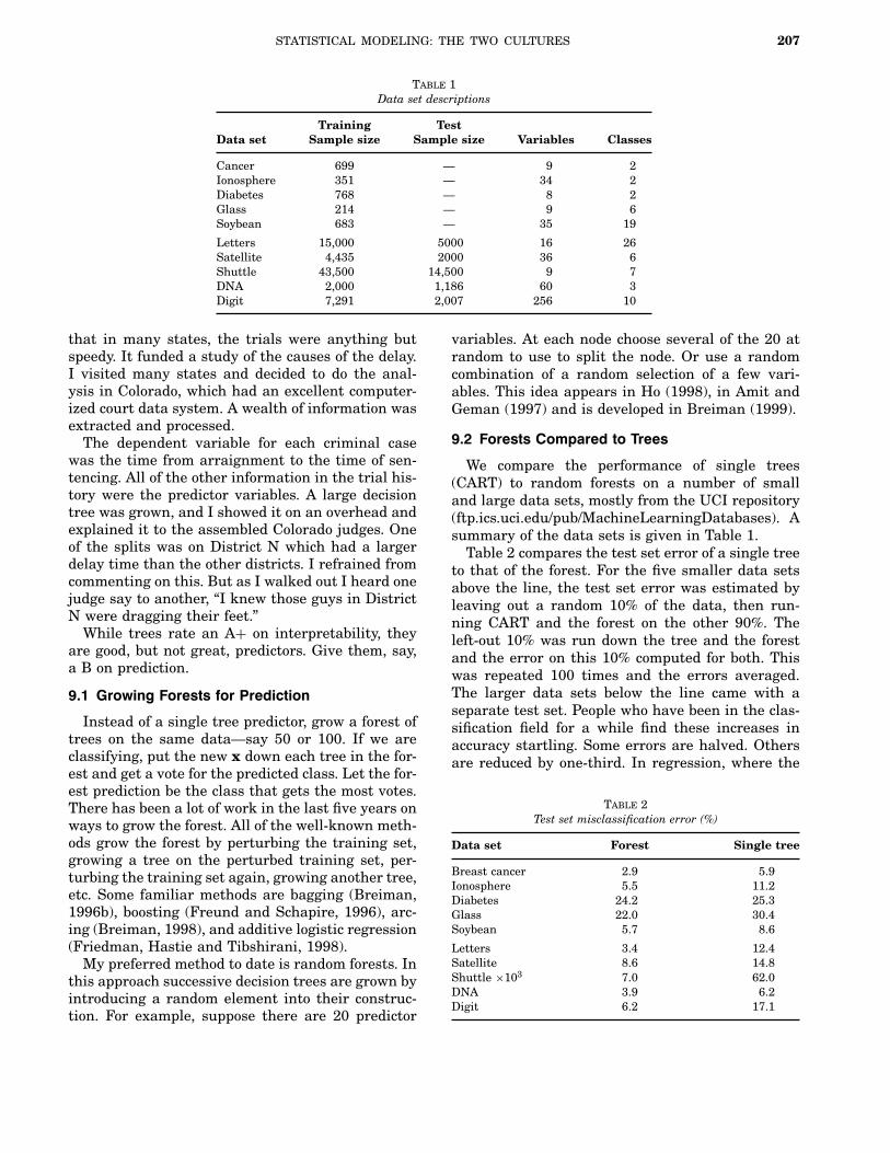
We compare the performance of single trees(CART) to random forests on a number of smalland large data sets, mostly from the UCI repository(ftp.ics.uci.edu/pub/MachineLearningDatabases). Asummary of the data sets is given in Table 1.Table 2 compares the test set error of a single tree

to that of the forest. For the five smaller data setsabove the line, the test set error was estimated byleaving out a random 10% of the data, then run-ning CART and the forest on the other 90%. Theleft-out 10% was run down the tree and the forestand the error on this 10% computed for both. Thiswas repeated 100 times and the errors averaged.The larger data sets below the line came with aseparate test set. People who have been in the clas-sification field for a while find these increases inaccuracy startling. Some errors are halved. Othersare reduced by one-third. In regression, where the

Table 2Test set misclassification error (%)

Data set Forest Single tree

Breast cancer 2.9 5.9Ionosphere 5.5 11.2Diabetes 24.2 25.3Glass 22.0 30.4Soybean 5.7 8.6

Letters 3.4 12.4Satellite 8.6 14.8Shuttle ×103 7.0 62.0DNA 3.9 6.2Digit 6.2 17.1

208 L. BREIMAN

forest prediction is the average over the individualtree predictions, the decreases in mean-squared testset error are similar.

9.3 Random Forests are A + Predictors

The Statlog Project (Mitchie, Spiegelhalter andTaylor, 1994) compared 18 different classifiers.Included were neural nets, CART, linear andquadratic discriminant analysis, nearest neighbor,etc. The first four data sets below the line in Table 1were the only ones used in the Statlog Project thatcame with separate test sets. In terms of rank ofaccuracy on these four data sets, the forest comesin 1, 1, 1, 1 for an average rank of 1.0. The nextbest classifier had an average rank of 7.3.The fifth data set below the line consists of 16×16

pixel gray scale depictions of handwritten ZIP Codenumerals. It has been extensively used by AT&TBell Labs to test a variety of prediction methods.A neural net handcrafted to the data got a test seterror of 5.1% vs. 6.2% for a standard run of randomforest.

9.4 The Occam Dilemma

So forests are A+ predictors. But their mechanismfor producing a prediction is difficult to understand.Trying to delve into the tangled web that generateda plurality vote from 100 trees is a Herculean task.So on interpretability, they rate an F. Which bringsus to the Occam dilemma:

• Accuracy generally requires more complex pre-diction methods. Simple and interpretable functionsdo not make the most accurate predictors.

Using complex predictors may be unpleasant, butthe soundest path is to go for predictive accuracyfirst, then try to understand why. In fact, Section10 points out that from a goal-oriented statisticalviewpoint, there is no Occam’s dilemma. (For moreon Occam’s Razor see Domingos, 1998, 1999.)

10. BELLMAN AND THE CURSE OFDIMENSIONALITY

The title of this section refers to Richard Bell-man’s famous phrase, “the curse of dimensionality.”For decades, the first step in prediction methodol-ogy was to avoid the curse. If there were too manyprediction variables, the recipe was to find a fewfeatures (functions of the predictor variables) that“contain most of the information” and then usethese features to replace the original variables. Inprocedures common in statistics such as regres-sion, logistic regression and survival models theadvised practice is to use variable deletion to reduce

the dimensionality. The published advice was thathigh dimensionality is dangerous. For instance, awell-regarded book on pattern recognition (Meisel,1972) states “the features� � � must be relativelyfew in number.” But recent work has shown thatdimensionality can be a blessing.

10.1 Digging It Out in Small Pieces

Reducing dimensionality reduces the amount ofinformation available for prediction. The more pre-dictor variables, the more information. There is alsoinformation in various combinations of the predictorvariables. Let’s try going in the opposite direction:

• Instead of reducing dimensionality, increase itby adding many functions of the predictor variables.

There may now be thousands of features. Eachpotentially contains a small amount of information.The problem is how to extract and put togetherthese little pieces of information. There are twooutstanding examples of work in this direction, TheShape Recognition Forest (Y. Amit and D. Geman,1997) and Support Vector Machines (V. Vapnik,1995, 1998).

10.2 The Shape Recognition Forest

In 1992, the National Institute of Standards andTechnology (NIST) set up a competition for machinealgorithms to read handwritten numerals. They puttogether a large set of pixel pictures of handwrittennumbers (223,000) written by over 2,000 individ-uals. The competition attracted wide interest, anddiverse approaches were tried.The Amit–Geman approach defined many thou-

sands of small geometric features in a hierarchi-cal assembly. Shallow trees are grown, such that ateach node, 100 features are chosen at random fromthe appropriate level of the hierarchy; and the opti-mal split of the node based on the selected featuresis found.When a pixel picture of a number is dropped down

a single tree, the terminal node it lands in givesprobability estimates p0 � � � p9 that it representsnumbers 01 � � � 9. Over 1,000 trees are grown, theprobabilities averaged over this forest, and the pre-dicted number is assigned to the largest averagedprobability.Using a 100,000 example training set and a

50,000 test set, the Amit–Geman method gives atest set error of 0.7%–close to the limits of humanerror.

10.3 Support Vector Machines

Suppose there is two-class data having predictionvectors inM-dimensional Euclidean space. The pre-diction vectors for class #1 are �x�1�� and those for

STATISTICAL MODELING: THE TWO CULTURES 209

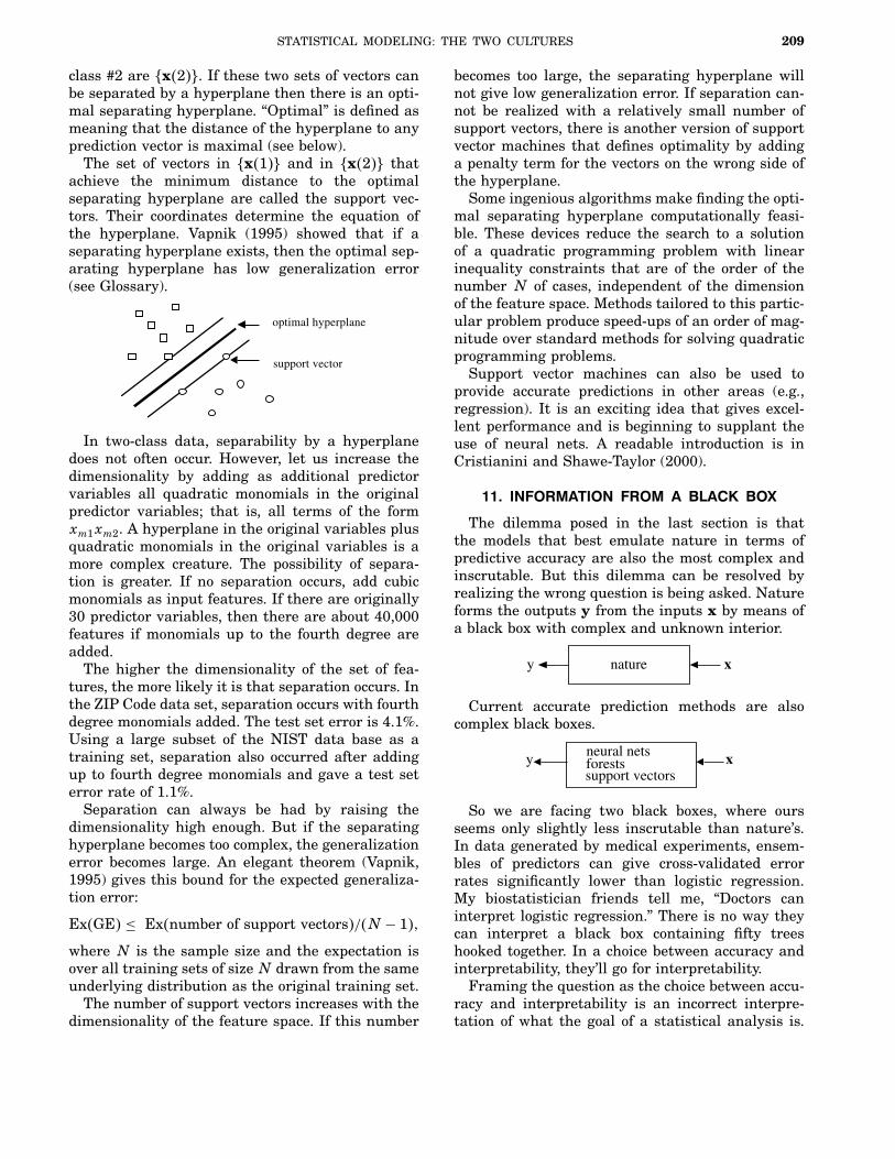
class #2 are �x�2��. If these two sets of vectors canbe separated by a hyperplane then there is an opti-mal separating hyperplane. “Optimal” is defined asmeaning that the distance of the hyperplane to anyprediction vector is maximal (see below).The set of vectors in �x�1�� and in �x�2�� that

achieve the minimum distance to the optimalseparating hyperplane are called the support vec-tors. Their coordinates determine the equation ofthe hyperplane. Vapnik (1995) showed that if aseparating hyperplane exists, then the optimal sep-arating hyperplane has low generalization error(see Glossary).

optimal hyperplane

support vector

In two-class data, separability by a hyperplanedoes not often occur. However, let us increase thedimensionality by adding as additional predictorvariables all quadratic monomials in the originalpredictor variables; that is, all terms of the formxm1xm2. A hyperplane in the original variables plusquadratic monomials in the original variables is amore complex creature. The possibility of separa-tion is greater. If no separation occurs, add cubicmonomials as input features. If there are originally30 predictor variables, then there are about 40,000features if monomials up to the fourth degree areadded.The higher the dimensionality of the set of fea-

tures, the more likely it is that separation occurs. Inthe ZIP Code data set, separation occurs with fourthdegree monomials added. The test set error is 4.1%.Using a large subset of the NIST data base as atraining set, separation also occurred after addingup to fourth degree monomials and gave a test seterror rate of 1.1%.Separation can always be had by raising the

dimensionality high enough. But if the separatinghyperplane becomes too complex, the generalizationerror becomes large. An elegant theorem (Vapnik,1995) gives this bound for the expected generaliza-tion error:

Ex�GE� ≤ Ex�number of support vectors�/�N− 1�where N is the sample size and the expectation isover all training sets of sizeN drawn from the sameunderlying distribution as the original training set.The number of support vectors increases with the

dimensionality of the feature space. If this number

becomes too large, the separating hyperplane willnot give low generalization error. If separation can-not be realized with a relatively small number ofsupport vectors, there is another version of supportvector machines that defines optimality by addinga penalty term for the vectors on the wrong side ofthe hyperplane.Some ingenious algorithms make finding the opti-

mal separating hyperplane computationally feasi-ble. These devices reduce the search to a solutionof a quadratic programming problem with linearinequality constraints that are of the order of thenumber N of cases, independent of the dimensionof the feature space. Methods tailored to this partic-ular problem produce speed-ups of an order of mag-nitude over standard methods for solving quadraticprogramming problems.Support vector machines can also be used to

provide accurate predictions in other areas (e.g.,regression). It is an exciting idea that gives excel-lent performance and is beginning to supplant theuse of neural nets. A readable introduction is inCristianini and Shawe-Taylor (2000).

11. INFORMATION FROM A BLACK BOX

The dilemma posed in the last section is thatthe models that best emulate nature in terms ofpredictive accuracy are also the most complex andinscrutable. But this dilemma can be resolved byrealizing the wrong question is being asked. Natureforms the outputs y from the inputs x by means ofa black box with complex and unknown interior.

y xnature

Current accurate prediction methods are alsocomplex black boxes.

y xneural nets forestssupport vectors

So we are facing two black boxes, where oursseems only slightly less inscrutable than nature’s.In data generated by medical experiments, ensem-bles of predictors can give cross-validated errorrates significantly lower than logistic regression.My biostatistician friends tell me, “Doctors caninterpret logistic regression.” There is no way theycan interpret a black box containing fifty treeshooked together. In a choice between accuracy andinterpretability, they’ll go for interpretability.Framing the question as the choice between accu-

racy and interpretability is an incorrect interpre-tation of what the goal of a statistical analysis is.

210 L. BREIMAN

The point of a model is to get useful informationabout the relation between the response and pre-dictor variables. Interpretability is a way of gettinginformation. But a model does not have to be simpleto provide reliable information about the relationbetween predictor and response variables; neitherdoes it have to be a data model.

• The goal is not interpretability, but accurateinformation.

The following three examples illustrate this point.The first shows that random forests applied to amedical data set can give more reliable informa-tion about covariate strengths than logistic regres-sion. The second shows that it can give interestinginformation that could not be revealed by a logisticregression. The third is an application to a microar-ray data where it is difficult to conceive of a datamodel that would uncover similar information.

11.1 Example I: Variable Importance in aSurvival Data Set

The data set contains survival or nonsurvivalof 155 hepatitis patients with 19 covariates. It isavailable at ftp.ics.uci.edu/pub/MachineLearning-Databases and was contributed by Gail Gong. Thedescription is in a file called hepatitis.names. Thedata set has been previously analyzed by Diaconisand Efron (1983), and Cestnik, Konenenko andBratko (1987). The lowest reported error rate todate, 17%, is in the latter paper.Diaconis and Efron refer to work by Peter Gre-

gory of the Stanford Medical School who analyzedthis data and concluded that the important vari-ables were numbers 6, 12, 14, 19 and reports an esti-mated 20% predictive accuracy. The variables werereduced in two stages—the first was by informaldata analysis. The second refers to a more formal

– . 5

.5

1.5

2.5

3.5

stan

dard

ized

coe

ffici

ents

0 1 2 3 4 5 6 7 8 9 1 0 1 1 1 2 1 3 1 4 1 5 1 6 1 7 1 8 1 9 2 0variables

Fig. 1. Standardized coefficients logistic regression.

(unspecified) statistical procedure which I assumewas logistic regression.Efron and Diaconis drew 500 bootstrap samples

from the original data set and used a similar pro-cedure to isolate the important variables in eachbootstrapped data set. The authors comment, “Ofthe four variables originally selected not one wasselected in more than 60 percent of the samples.Hence the variables identified in the original analy-sis cannot be taken too seriously.” We will come backto this conclusion later.

Logistic Regression

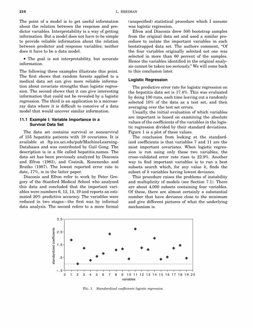
The predictive error rate for logistic regression onthe hepatitis data set is 17.4%. This was evaluatedby doing 100 runs, each time leaving out a randomlyselected 10% of the data as a test set, and thenaveraging over the test set errors.Usually, the initial evaluation of which variables

are important is based on examining the absolutevalues of the coefficients of the variables in the logis-tic regression divided by their standard deviations.Figure 1 is a plot of these values.The conclusion from looking at the standard-

ized coefficients is that variables 7 and 11 are themost important covariates. When logistic regres-sion is run using only these two variables, thecross-validated error rate rises to 22.9%. Anotherway to find important variables is to run a bestsubsets search which, for any value k, finds thesubset of k variables having lowest deviance.This procedure raises the problems of instability

and multiplicity of models (see Section 7.1). Thereare about 4,000 subsets containing four variables.Of these, there are almost certainly a substantialnumber that have deviance close to the minimumand give different pictures of what the underlyingmechanism is.

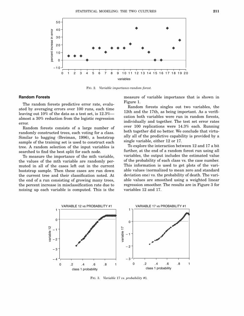
STATISTICAL MODELING: THE TWO CULTURES 211

– 1 0

0

1 0

2 0

3 0

4 0

5 0

perc

ent i

ncre

se in

err

or

0 1 2 3 4 5 6 7 8 9 1 0 1 1 1 2 1 3 1 4 1 5 1 6 1 7 1 8 1 9 2 0

variables

Fig. 2. Variable importance-random forest.

Random Forests

The random forests predictive error rate, evalu-ated by averaging errors over 100 runs, each timeleaving out 10% of the data as a test set, is 12.3%—almost a 30% reduction from the logistic regressionerror.Random forests consists of a large number of

randomly constructed trees, each voting for a class.Similar to bagging (Breiman, 1996), a bootstrapsample of the training set is used to construct eachtree. A random selection of the input variables issearched to find the best split for each node.To measure the importance of the mth variable,

the values of the mth variable are randomly per-muted in all of the cases left out in the currentbootstrap sample. Then these cases are run downthe current tree and their classification noted. Atthe end of a run consisting of growing many trees,the percent increase in misclassification rate due tonoising up each variable is computed. This is the

– 4

– 3

– 2

– 1

0

1

varia

ble

12

0 . 2 .4 .6 .8 1

class 1 probability

VARIABLE 12 vs PROBABILITY #1

– 3

– 2

– 1

0

1

varia

ble

17

0 . 2 .4 .6 .8 1class 1 probability

VARIABLE 17 vs PROBABILITY #1

Fig. 3. Variable 17 vs. probability #1.

measure of variable importance that is shown inFigure 1.Random forests singles out two variables, the

12th and the 17th, as being important. As a verifi-cation both variables were run in random forests,individually and together. The test set error ratesover 100 replications were 14.3% each. Runningboth together did no better. We conclude that virtu-ally all of the predictive capability is provided by asingle variable, either 12 or 17.To explore the interaction between 12 and 17 a bit

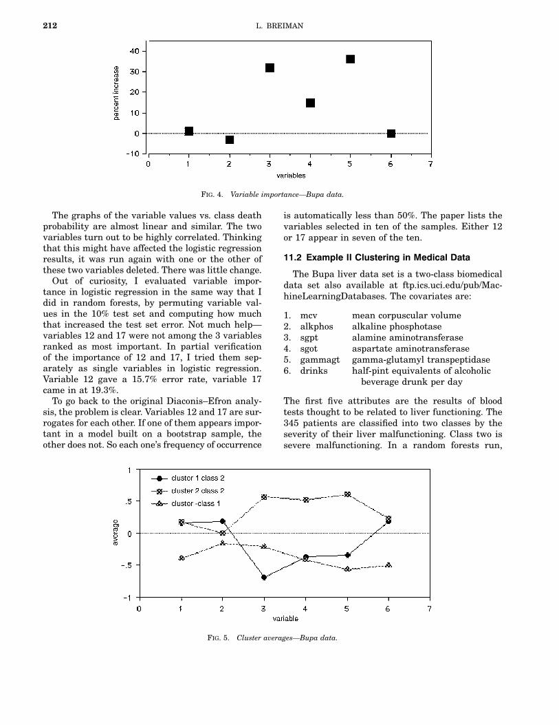
further, at the end of a random forest run using allvariables, the output includes the estimated valueof the probability of each class vs. the case number.This information is used to get plots of the vari-able values (normalized to mean zero and standarddeviation one) vs. the probability of death. The vari-able values are smoothed using a weighted linearregression smoother. The results are in Figure 3 forvariables 12 and 17.

212 L. BREIMAN

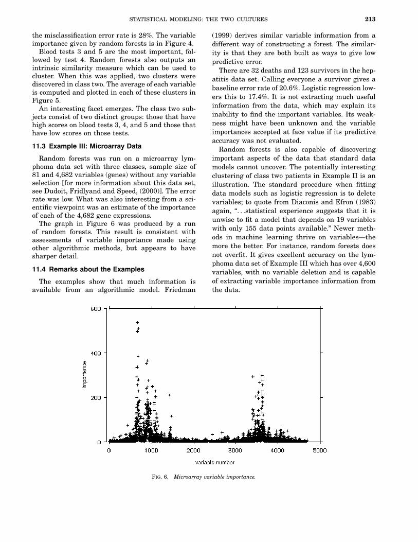
Fig. 4. Variable importance—Bupa data.

The graphs of the variable values vs. class deathprobability are almost linear and similar. The twovariables turn out to be highly correlated. Thinkingthat this might have affected the logistic regressionresults, it was run again with one or the other ofthese two variables deleted. There was little change.Out of curiosity, I evaluated variable impor-

tance in logistic regression in the same way that Idid in random forests, by permuting variable val-ues in the 10% test set and computing how muchthat increased the test set error. Not much help—variables 12 and 17 were not among the 3 variablesranked as most important. In partial verificationof the importance of 12 and 17, I tried them sep-arately as single variables in logistic regression.Variable 12 gave a 15.7% error rate, variable 17came in at 19.3%.To go back to the original Diaconis–Efron analy-

sis, the problem is clear. Variables 12 and 17 are sur-rogates for each other. If one of them appears impor-tant in a model built on a bootstrap sample, theother does not. So each one’s frequency of occurrence

Fig. 5. Cluster averages—Bupa data.

is automatically less than 50%. The paper lists thevariables selected in ten of the samples. Either 12or 17 appear in seven of the ten.

11.2 Example II Clustering in Medical Data

The Bupa liver data set is a two-class biomedicaldata set also available at ftp.ics.uci.edu/pub/Mac-hineLearningDatabases. The covariates are:

1. mcv mean corpuscular volume2. alkphos alkaline phosphotase3. sgpt alamine aminotransferase4. sgot aspartate aminotransferase5. gammagt gamma-glutamyl transpeptidase6. drinks half-pint equivalents of alcoholic

beverage drunk per day

The first five attributes are the results of bloodtests thought to be related to liver functioning. The345 patients are classified into two classes by theseverity of their liver malfunctioning. Class two issevere malfunctioning. In a random forests run,

STATISTICAL MODELING: THE TWO CULTURES 213

the misclassification error rate is 28%. The variableimportance given by random forests is in Figure 4.Blood tests 3 and 5 are the most important, fol-

lowed by test 4. Random forests also outputs anintrinsic similarity measure which can be used tocluster. When this was applied, two clusters werediscovered in class two. The average of each variableis computed and plotted in each of these clusters inFigure 5.An interesting facet emerges. The class two sub-

jects consist of two distinct groups: those that havehigh scores on blood tests 3, 4, and 5 and those thathave low scores on those tests.

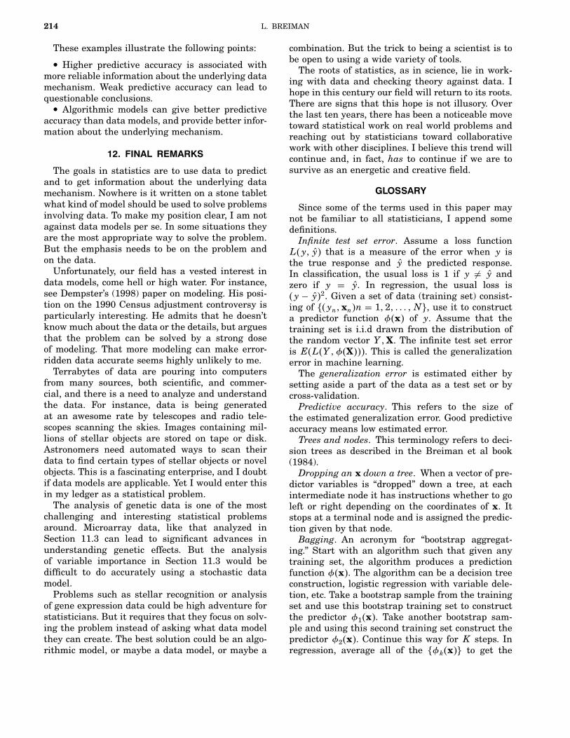
11.3 Example III: Microarray Data

Random forests was run on a microarray lym-phoma data set with three classes, sample size of81 and 4,682 variables (genes) without any variableselection [for more information about this data set,see Dudoit, Fridlyand and Speed, (2000)]. The errorrate was low. What was also interesting from a sci-entific viewpoint was an estimate of the importanceof each of the 4,682 gene expressions.The graph in Figure 6 was produced by a run

of random forests. This result is consistent withassessments of variable importance made usingother algorithmic methods, but appears to havesharper detail.

11.4 Remarks about the Examples

The examples show that much information isavailable from an algorithmic model. Friedman

Fig. 6. Microarray variable importance.

(1999) derives similar variable information from adifferent way of constructing a forest. The similar-ity is that they are both built as ways to give lowpredictive error.There are 32 deaths and 123 survivors in the hep-

atitis data set. Calling everyone a survivor gives abaseline error rate of 20.6%. Logistic regression low-ers this to 17.4%. It is not extracting much usefulinformation from the data, which may explain itsinability to find the important variables. Its weak-ness might have been unknown and the variableimportances accepted at face value if its predictiveaccuracy was not evaluated.Random forests is also capable of discovering

important aspects of the data that standard datamodels cannot uncover. The potentially interestingclustering of class two patients in Example II is anillustration. The standard procedure when fittingdata models such as logistic regression is to deletevariables; to quote from Diaconis and Efron (1983)again, “� � �statistical experience suggests that it isunwise to fit a model that depends on 19 variableswith only 155 data points available.” Newer meth-ods in machine learning thrive on variables—themore the better. For instance, random forests doesnot overfit. It gives excellent accuracy on the lym-phoma data set of Example III which has over 4,600variables, with no variable deletion and is capableof extracting variable importance information fromthe data.

214 L. BREIMAN

These examples illustrate the following points:

• Higher predictive accuracy is associated withmore reliable information about the underlying datamechanism. Weak predictive accuracy can lead toquestionable conclusions.• Algorithmic models can give better predictive

accuracy than data models, and provide better infor-mation about the underlying mechanism.

12. FINAL REMARKS

The goals in statistics are to use data to predictand to get information about the underlying datamechanism. Nowhere is it written on a stone tabletwhat kind of model should be used to solve problemsinvolving data. To make my position clear, I am notagainst data models per se. In some situations theyare the most appropriate way to solve the problem.But the emphasis needs to be on the problem andon the data.Unfortunately, our field has a vested interest in

data models, come hell or high water. For instance,see Dempster’s (1998) paper on modeling. His posi-tion on the 1990 Census adjustment controversy isparticularly interesting. He admits that he doesn’tknow much about the data or the details, but arguesthat the problem can be solved by a strong doseof modeling. That more modeling can make error-ridden data accurate seems highly unlikely to me.Terrabytes of data are pouring into computers

from many sources, both scientific, and commer-cial, and there is a need to analyze and understandthe data. For instance, data is being generatedat an awesome rate by telescopes and radio tele-scopes scanning the skies. Images containing mil-lions of stellar objects are stored on tape or disk.Astronomers need automated ways to scan theirdata to find certain types of stellar objects or novelobjects. This is a fascinating enterprise, and I doubtif data models are applicable. Yet I would enter thisin my ledger as a statistical problem.The analysis of genetic data is one of the most

challenging and interesting statistical problemsaround. Microarray data, like that analyzed inSection 11.3 can lead to significant advances inunderstanding genetic effects. But the analysisof variable importance in Section 11.3 would bedifficult to do accurately using a stochastic datamodel.Problems such as stellar recognition or analysis

of gene expression data could be high adventure forstatisticians. But it requires that they focus on solv-ing the problem instead of asking what data modelthey can create. The best solution could be an algo-rithmic model, or maybe a data model, or maybe a

combination. But the trick to being a scientist is tobe open to using a wide variety of tools.The roots of statistics, as in science, lie in work-

ing with data and checking theory against data. Ihope in this century our field will return to its roots.There are signs that this hope is not illusory. Overthe last ten years, there has been a noticeable movetoward statistical work on real world problems andreaching out by statisticians toward collaborativework with other disciplines. I believe this trend willcontinue and, in fact, has to continue if we are tosurvive as an energetic and creative field.

GLOSSARY

Since some of the terms used in this paper maynot be familiar to all statisticians, I append somedefinitions.Infinite test set error. Assume a loss function

L�y y� that is a measure of the error when y isthe true response and y the predicted response.In classification, the usual loss is 1 if y = y andzero if y = y. In regression, the usual loss is�y − y�2. Given a set of data (training set) consist-ing of ��ynxn�n = 12 � � � N�, use it to constructa predictor function φ�x� of y. Assume that thetraining set is i.i.d drawn from the distribution ofthe random vector YX. The infinite test set erroris E�L�Yφ�X���. This is called the generalizationerror in machine learning.The generalization error is estimated either by

setting aside a part of the data as a test set or bycross-validation.Predictive accuracy. This refers to the size of

the estimated generalization error. Good predictiveaccuracy means low estimated error.Trees and nodes. This terminology refers to deci-

sion trees as described in the Breiman et al book(1984).Dropping an x down a tree. When a vector of pre-

dictor variables is “dropped” down a tree, at eachintermediate node it has instructions whether to goleft or right depending on the coordinates of x. Itstops at a terminal node and is assigned the predic-tion given by that node.Bagging. An acronym for “bootstrap aggregat-

ing.” Start with an algorithm such that given anytraining set, the algorithm produces a predictionfunction φ�x�. The algorithm can be a decision treeconstruction, logistic regression with variable dele-tion, etc. Take a bootstrap sample from the trainingset and use this bootstrap training set to constructthe predictor φ1�x�. Take another bootstrap sam-ple and using this second training set construct thepredictor φ2�x�. Continue this way for K steps. Inregression, average all of the �φk�x�� to get the

STATISTICAL MODELING: THE TWO CULTURES 215

bagged predictor at x. In classification, that classwhich has the plurality vote of the �φk�x�� is thebagged predictor. Bagging has been shown effectivein variance reduction (Breiman, 1996b).Boosting. This is a more complex way of forming

an ensemble of predictors in classification than bag-ging (Freund and Schapire, 1996). It uses no ran-domization but proceeds by altering the weights onthe training set. Its performance in terms of low pre-diction error is excellent (for details see Breiman,1998).

ACKNOWLEDGMENTS

Many of my ideas about data modeling wereformed in three decades of conversations with myold friend and collaborator, Jerome Friedman. Con-versations with Richard Olshen about the Coxmodel and its use in biostatistics helped me tounderstand the background. I am also indebted toWilliam Meisel, who headed some of the predic-tion projects I consulted on and helped me makethe transition from probability theory to algorithms,and to Charles Stone for illuminating conversationsabout the nature of statistics and science. I’m grate-ful also for the comments of the editor, Leon Gleser,which prompted a major rewrite of the first draftof this manuscript and resulted in a different andbetter paper.

REFERENCES

Amit, Y. and Geman, D. (1997). Shape quantization and recog-nition with randomized trees. Neural Computation 9 1545–1588.

Arena, C., Sussman, N., Chiang, K., Mazumdar, S., Macina,O. and Li, W. (2000). Bagging Structure-Activity Rela-tionships: A simulation study for assessing misclassifica-tion rates. Presented at the Second Indo-U.S. Workshop onMathematical Chemistry, Duluth, MI. (Available at NSuss-man@server.ceoh.pitt.edu).

Bickel, P., Ritov, Y. and Stoker, T. (2001). Tailor-made testsfor goodness of fit for semiparametric hypotheses. Unpub-lished manuscript.

Breiman, L. (1996a). The heuristics of instability in model selec-tion. Ann. Statist. 24 2350–2381.

Breiman, L. (1996b). Bagging predictors. Machine Learning J.26 123–140.

Breiman, L. (1998). Arcing classifiers. Discussion paper, Ann.Statist. 26 801–824.

Breiman. L. (2000). Some infinity theory for tree ensembles.(Available at www.stat.berkeley.edu/technical reports).

Breiman, L. (2001). Random forests. Machine Learning J. 45 5–32.

Breiman, L. and Friedman, J. (1985). Estimating optimal trans-formations in multiple regression and correlation. J. Amer.Statist. Assoc. 80 580–619.

Breiman, L., Friedman, J., Olshen, R. and Stone, C.(1984). Classification and Regression Trees. Wadsworth,Belmont, CA.

Cristianini, N. and Shawe-Taylor, J. (2000). An Introductionto Support Vector Machines. Cambridge Univ. Press.

Daniel, C. andWood, F. (1971). Fitting equations to data. Wiley,New York.

Dempster, A. (1998). Logicist statistic 1. Models and Modeling.Statist. Sci. 13 3 248–276.

Diaconis, P. and Efron, B. (1983). Computer intensive methodsin statistics. Scientific American 248 116–131.

Domingos, P. (1998). Occam’s two razors: the sharp and theblunt. In Proceedings of the Fourth International Conferenceon Knowledge Discovery and Data Mining (R. Agrawal andP. Stolorz, eds.) 37–43. AAAI Press, Menlo Park, CA.

Domingos, P. (1999). The role of Occam’s razor in knowledge dis-covery. Data Mining and Knowledge Discovery 3 409–425.

Dudoit, S., Fridlyand, J. and Speed, T. (2000). Comparisonof discrimination methods for the classification of tumors.(Available at www.stat.berkeley.edu/technical reports).

Freedman, D. (1987). As others see us: a case study in pathanalysis (with discussion). J. Ed. Statist. 12 101–223.

Freedman, D. (1991). Statistical models and shoe leather. Soci-ological Methodology 1991 (with discussion) 291–358.

Freedman, D. (1991). Some issues in the foundations of statis-tics. Foundations of Science 1 19–83.

Freedman, D. (1994). From association to causation via regres-sion. Adv. in Appl. Math. 18 59–110.

Freund, Y. and Schapire, R. (1996). Experiments with a newboosting algorithm. In Machine Learning: Proceedings of theThirteenth International Conference 148–156. Morgan Kauf-mann, San Francisco.

Friedman, J. (1999). Greedy predictive approximation: a gra-dient boosting machine. Technical report, Dept. StatisticsStanford Univ.

Friedman, J., Hastie, T. and Tibshirani, R. (2000). Additivelogistic regression: a statistical view of boosting. Ann. Statist.28 337–407.

Gifi, A. (1990). Nonlinear Multivariate Analysis. Wiley, NewYork.

Ho, T. K. (1998). The random subspace method for constructingdecision forests. IEEE Trans. Pattern Analysis and MachineIntelligence 20 832–844.

Landswher, J., Preibon, D. and Shoemaker, A. (1984). Graph-ical methods for assessing logistic regression models (withdiscussion). J. Amer. Statist. Assoc. 79 61–83.

McCullagh, P. and Nelder, J. (1989). Generalized Linear Mod-els. Chapman and Hall, London.

Meisel, W. (1972). Computer-Oriented Approaches to PatternRecognition. Academic Press, New York.

Michie, D., Spiegelhalter, D. and Taylor, C. (1994). MachineLearning, Neural and Statistical Classification. Ellis Hor-wood, New York.

Mosteller, F. and Tukey, J. (1977). Data Analysis and Regres-sion. Addison-Wesley, Redding, MA.

Mountain, D. and Hsiao, C. (1989). A combined structural andflexible functional approach for modelenery substitution.J. Amer. Statist. Assoc. 84 76–87.

Stone, M. (1974). Cross-validatory choice and assessment of sta-tistical predictions. J. Roy. Statist. Soc. B 36 111–147.

Vapnik, V. (1995). The Nature of Statistical Learning Theory.Springer, New York.

Vapnik, V (1998). Statistical Learning Theory. Wiley, New York.Wahba, G. (1990). Spline Models for Observational Data. SIAM,

Philadelphia.Zhang, H. and Singer, B. (1999). Recursive Partitioning in the

Health Sciences. Springer, New York.

216 L. BREIMAN

CommentD. R. Cox

Professor Breiman’s interesting paper gives botha clear statement of the broad approach underly-ing some of his influential and widely admired con-tributions and outlines some striking applicationsand developments. He has combined this with a cri-tique of what, for want of a better term, I will callmainstream statistical thinking, based in part ona caricature. Like all good caricatures, it containsenough truth and exposes enough weaknesses to bethought-provoking.There is not enough space to comment on all the

many points explicitly or implicitly raised in thepaper. There follow some remarks about a few mainissues.One of the attractions of our subject is the aston-

ishingly wide range of applications as judged notonly in terms of substantive field but also in termsof objectives, quality and quantity of data andso on. Thus any unqualified statement that “inapplications� � �” has to be treated sceptically. Oneof our failings has, I believe, been, in a wish tostress generality, not to set out more clearly thedistinctions between different kinds of applicationand the consequences for the strategy of statisticalanalysis. Of course we have distinctions betweendecision-making and inference, between tests andestimation, and between estimation and predic-tion and these are useful but, I think, are, exceptperhaps the first, too phrased in terms of the tech-nology rather than the spirit of statistical analysis.I entirely agree with Professor Breiman that itwould be an impoverished and extremely unhis-torical view of the subject to exclude the kind ofwork he describes simply because it has no explicitprobabilistic base.Professor Breiman takes data as his starting

point. I would prefer to start with an issue, a ques-tion or a scientific hypothesis, although I wouldbe surprised if this were a real source of disagree-ment. These issues may evolve, or even changeradically, as analysis proceeds. Data looking fora question are not unknown and raise puzzlesbut are, I believe, atypical in most contexts. Next,even if we ignore design aspects and start with data,

D. R. Cox is an Honorary Fellow, Nuffield College,Oxford OX1 1NF, United Kingdom, and associatemember, Department of Statistics, University ofOxford (e-mail: david.cox@nuffield.oxford.ac.uk).

key points concern the precise meaning of the data,the possible biases arising from the method of ascer-tainment, the possible presence of major distortingmeasurement errors and the nature of processesunderlying missing and incomplete data and datathat evolve in time in a way involving complex inter-dependencies. For some of these, at least, it is hardto see how to proceed without some notion of prob-abilistic modeling.Next Professor Breiman emphasizes prediction

as the objective, success at prediction being thecriterion of success, as contrasted with issuesof interpretation or understanding. Prediction isindeed important from several perspectives. Thesuccess of a theory is best judged from its ability topredict in new contexts, although one cannot dis-miss as totally useless theories such as the rationalaction theory (RAT), in political science, which, asI understand it, gives excellent explanations of thepast but which has failed to predict the real politi-cal world. In a clinical trial context it can be arguedthat an objective is to predict the consequences oftreatment allocation to future patients, and so on.If the prediction is localized to situations directly

similar to those applying to the data there is thenan interesting and challenging dilemma. Is it prefer-able to proceed with a directly empirical black-boxapproach, as favored by Professor Breiman, or isit better to try to take account of some underly-ing explanatory process? The answer must dependon the context but I certainly accept, although itgoes somewhat against the grain to do so, thatthere are situations where a directly empiricalapproach is better. Short term economic forecastingand real-time flood forecasting are probably furtherexemplars. Key issues are then the stability of thepredictor as practical prediction proceeds, the needfrom time to time for recalibration and so on.However, much prediction is not like this. Often

the prediction is under quite different conditionsfrom the data; what is the likely progress of theincidence of the epidemic of v-CJD in the UnitedKingdom, what would be the effect on annual inci-dence of cancer in the United States of reducing by10% the medical use of X-rays, etc.? That is, it maybe desired to predict the consequences of somethingonly indirectly addressed by the data available foranalysis. As we move toward such more ambitioustasks, prediction, always hazardous, without someunderstanding of underlying process and linkingwith other sources of information, becomes more

STATISTICAL MODELING: THE TWO CULTURES 217

and more tentative. Formulation of the goals ofanalysis solely in terms of direct prediction over thedata set seems then increasingly unhelpful.This is quite apart from matters where the direct

objective is understanding of and tests of subject-matter hypotheses about underlying process, thenature of pathways of dependence and so on.What is the central strategy of mainstream sta-

tistical analysis? This can most certainly not be dis-cerned from the pages of Bernoulli, The Annals ofStatistics or the Scandanavian Journal of Statisticsnor from Biometrika and the Journal of Royal Sta-tistical Society, Series B or even from the applicationpages of Journal of the American Statistical Associa-tion or Applied Statistics, estimable though all thesejournals are. Of course as we move along the list,there is an increase from zero to 100% in the paperscontaining analyses of “real” data. But the papersdo so nearly always to illustrate technique ratherthan to explain the process of analysis and inter-pretation as such. This is entirely legitimate, butis completely different from live analysis of currentdata to obtain subject-matter conclusions or to helpsolve specific practical issues. Put differently, if animportant conclusion is reached involving statisti-cal analysis it will be reported in a subject-matterjournal or in a written or verbal report to colleagues,government or business. When that happens, statis-tical details are typically and correctly not stressed.Thus the real procedures of statistical analysis canbe judged only by looking in detail at specific cases,and access to these is not always easy. Failure todiscuss enough the principles involved is a majorcriticism of the current state of theory.I think tentatively that the following quite com-

monly applies. Formal models are useful and oftenalmost, if not quite, essential for incisive thinking.Descriptively appealing and transparent methodswith a firm model base are the ideal. Notions ofsignificance tests, confidence intervals, posteriorintervals and all the formal apparatus of inferenceare valuable tools to be used as guides, but not in amechanical way; they indicate the uncertainty thatwould apply under somewhat idealized, may bevery idealized, conditions and as such are oftenlower bounds to real uncertainty. Analyses andmodel development are at least partly exploratory.Automatic methods of model selection (and of vari-able selection in regression-like problems) are to beshunned or, if use is absolutely unavoidable, are tobe examined carefully for their effect on the finalconclusions. Unfocused tests of model adequacy arerarely helpful.By contrast, Professor Breiman equates main-

stream applied statistics to a relatively mechanical

process involving somehow or other choosing amodel, often a default model of standard form,and applying standard methods of analysis andgoodness-of-fit procedures. Thus for survival datachoose a priori the proportional hazards model.(Note, incidentally, that in the paper, often quotedbut probably rarely read, that introduced thisapproach there was a comparison of several of themany different models that might be suitable forthis kind of data.) It is true that many of the anal-yses done by nonstatisticians or by statisticiansunder severe time constraints are more or less likethose Professor Breiman describes. The issue thenis not whether they could ideally be improved, butwhether they capture enough of the essence of theinformation in the data, together with some rea-sonable indication of precision as a guard againstunder or overinterpretation. Would more refinedanalysis, possibly with better predictive power andbetter fit, produce subject-matter gains? There canbe no general answer to this, but one suspects thatquite often the limitations of conclusions lie morein weakness of data quality and study design thanin ineffective analysis.There are two broad lines of development active

at the moment arising out of mainstream statisticalideas. The first is the invention of models stronglytied to subject-matter considerations, represent-ing underlying dependencies, and their analysis,perhaps by Markov chain Monte Carlo methods.In fields where subject-matter considerations arelargely qualitative, we see a development based onMarkov graphs and their generalizations. Thesemethods in effect assume, subject in principle toempirical test, more and more about the phenom-ena under study. By contrast, there is an emphasison assuming less and less via, for example, kernelestimates of regression functions, generalized addi-tive models and so on. There is a need to be clearerabout the circumstances favoring these two broadapproaches, synthesizing them where possible.My own interest tends to be in the former style

of work. From this perspective Cox and Wermuth(1996, page 15) listed a number of requirements of astatistical model. These are to establish a link withbackground knowledge and to set up a connectionwith previous work, to give some pointer towarda generating process, to have primary parameterswith individual clear subject-matter interpretations,to specify haphazard aspects well enough to leadto meaningful assessment of precision and, finally,that the fit should be adequate. From this perspec-tive, fit, which is broadly related to predictive suc-cess, is not the primary basis for model choice andformal methods of model choice that take no account

218 L. BREIMAN

of the broader objectives are suspect in the presentcontext. In a sense these are efforts to establish datadescriptions that are potentially causal, recognizingthat causality, in the sense that a natural scientistwould use the term, can rarely be established fromone type of study and is at best somewhat tentative.Professor Breiman takes a rather defeatist atti-

tude toward attempts to formulate underlyingprocesses; is this not to reject the base of much sci-entific progress? The interesting illustrations givenby Beveridge (1952), where hypothesized processesin various biological contexts led to importantprogress, even though the hypotheses turned out inthe end to be quite false, illustrate the subtlety ofthe matter. Especially in the social sciences, repre-sentations of underlying process have to be viewedwith particular caution, but this does not makethem fruitless.The absolutely crucial issue in serious main-

stream statistics is the choice of a model thatwill translate key subject-matter questions into aform for analysis and interpretation. If a simplestandard model is adequate to answer the subject-matter question, this is fine: there are severehidden penalties for overelaboration. The statisti-cal literature, however, concentrates on how to do

the analysis, an important and indeed fascinatingquestion, but a secondary step. Better a roughanswer to the right question than an exact answerto the wrong question, an aphorism, due perhaps toLord Kelvin, that I heard as an undergraduate inapplied mathematics.I have stayed away from the detail of the paper

but will comment on just one point, the interestingtheorem of Vapnik about complete separation. Thisconfirms folklore experience with empirical logisticregression that, with a largish number of explana-tory variables, complete separation is quite likely tooccur. It is interesting that in mainstream thinkingthis is, I think, regarded as insecure in that com-plete separation is thought to be a priori unlikelyand the estimated separating plane unstable. Pre-sumably bootstrap and cross-validation ideas maygive here a quite misleading illusion of stability.Of course if the complete separator is subtle andstable Professor Breiman’s methods will emerge tri-umphant and ultimately it is an empirical questionin each application as to what happens.It will be clear that while I disagree with the main

thrust of Professor Breiman’s paper I found it stim-ulating and interesting.

CommentBrad Efron

At first glance Leo Breiman’s stimulating paperlooks like an argument against parsimony and sci-entific insight, and in favor of black boxes with lotsof knobs to twiddle. At second glance it still looksthat way, but the paper is stimulating, and Leo hassome important points to hammer home. At the riskof distortion I will try to restate one of those points,the most interesting one in my opinion, using lessconfrontational and more historical language.From the point of view of statistical development

the twentieth century might be labeled “100 yearsof unbiasedness.” Following Fisher’s lead, most ofour current statistical theory and practice revolvesaround unbiased or nearly unbiased estimates (par-ticularly MLEs), and tests based on such estimates.The power of this theory has made statistics the

Brad Efron is Professor, Department of Statis-tics, Sequoia Hall, 390 Serra Mall, Stanford Uni-versity, Stanford, California 94305–4065 (e-mail:brad@stat.stanford.edu).

dominant interpretational methodology in dozens offields, but, as we say in California these days, itis power purchased at a price: the theory requires amodestly high ratio of signal to noise, sample size tonumber of unknown parameters, to have much hopeof success. “Good experimental design” amounts toenforcing favorable conditions for unbiased estima-tion and testing, so that the statistician won’t findhimself or herself facing 100 data points and 50parameters.Now it is the twenty-first century when, as the

paper reminds us, we are being asked to face prob-lems that never heard of good experimental design.Sample sizes have swollen alarmingly while goalsgrow less distinct (“find interesting data structure”).New algorithms have arisen to deal with new prob-lems, a healthy sign it seems to me even if the inno-vators aren’t all professional statisticians. There areenough physicists to handle the physics case load,but there are fewer statisticians and more statisticsproblems, and we need all the help we can get. An

STATISTICAL MODELING: THE TWO CULTURES 219

attractive feature of Leo’s paper is his openness tonew ideas whatever their source.The new algorithms often appear in the form of

black boxes with enormous numbers of adjustableparameters (“knobs to twiddle”), sometimes moreknobs than data points. These algorithms can bequite successful as Leo points outs, sometimesmore so than their classical counterparts. However,unless the bias-variance trade-off has been sus-pended to encourage new statistical industries, theirsuccess must hinge on some form of biased estima-tion. The bias may be introduced directly as with the“regularization” of overparameterized linear mod-els, more subtly as in the pruning of overgrownregression trees, or surreptitiously as with supportvector machines, but it has to be lurking somewhereinside the theory.Of course the trouble with biased estimation is

that we have so little theory to fall back upon.Fisher’s information bound, which tells us how wella (nearly) unbiased estimator can possibly perform,is of no help at all in dealing with heavily biasedmethodology. Numerical experimentation by itself,unguided by theory, is prone to faddish wandering:Rule 1. New methods always look better than old

ones. Neural nets are better than logistic regres-sion, support vector machines are better than neu-ral nets, etc. In fact it is very difficult to run anhonest simulation comparison, and easy to inadver-tently cheat by choosing favorable examples, or bynot putting as much effort into optimizing the dullold standard as the exciting new challenger.Rule 2. Complicated methods are harder to crit-

icize than simple ones. By now it is easy to checkthe efficiency of a logistic regression, but it is nosmall matter to analyze the limitations of a sup-port vector machine. One of the best things statis-ticians do, and something that doesn’t happen out-side our profession, is clarify the inferential basisof a proposed new methodology, a nice recent exam-ple being Friedman, Hastie, and Tibshirani’s anal-ysis of “boosting,” (2000). The past half-century hasseen the clarification process successfully at work onnonparametrics, robustness and survival analysis.There has even been some success with biased esti-mation in the form of Stein shrinkage and empiricalBayes, but I believe the hardest part of this workremains to be done. Papers like Leo’s are a call formore analysis and theory, not less.Prediction is certainly an interesting subject but

Leo’s paper overstates both its role and our profes-sion’s lack of interest in it.

• The “prediction culture,” at least around Stan-ford, is a lot bigger than 2%, though its constituencychanges and most of us wouldn’t welcome beingtypecast.• Estimation and testing are a form of prediction:

“In our sample of 20 patients drug A outperformeddrug B; would this still be true if we went on to testall possible patients?”• Prediction by itself is only occasionally suffi-

cient. The post office is happy with any methodthat predicts correct addresses from hand-writtenscrawls. Peter Gregory undertook his study for pre-diction purposes, but also to better understand themedical basis of hepatitis. Most statistical surveyshave the identification of causal factors as their ulti-mate goal.

The hepatitis data was first analyzed by GailGong in her 1982 Ph.D. thesis, which concerned pre-diction problems and bootstrap methods for improv-ing on cross-validation. (Cross-validation itself is anuncertain methodology that deserves further crit-ical scrutiny; see, for example, Efron and Tibshi-rani, 1996). The Scientific American discussion isquite brief, a more thorough description appearingin Efron and Gong (1983). Variables 12 or 17 (13or 18 in Efron and Gong’s numbering) appearedas “important” in 60% of the bootstrap simulations,which might be compared with the 59% for variable19, the most for any single explanator.In what sense are variable 12 or 17 or 19

“important” or “not important”? This is the kind ofinteresting inferential question raised by predictionmethodology. Tibshirani and I made a stab at ananswer in our 1998 annals paper. I believe that thecurrent interest in statistical prediction will eventu-ally invigorate traditional inference, not eliminateit.A third front seems to have been opened in

the long-running frequentist-Bayesian wars by theadvocates of algorithmic prediction, who don’t reallybelieve in any inferential school. Leo’s paper is at itsbest when presenting the successes of algorithmicmodeling, which comes across as a positive devel-opment for both statistical practice and theoreticalinnovation. This isn’t an argument against tradi-tional data modeling any more than splines are anargument against polynomials. The whole point ofscience is to open up black boxes, understand theirinsides, and build better boxes for the purposes ofmankind. Leo himself is a notably successful sci-entist, so we can hope that the present paper waswritten more as an advocacy device than as the con-fessions of a born-again black boxist.

220 L. BREIMAN

CommentBruce Hoadley

INTRODUCTION

Professor Breiman’s paper is an important onefor statisticians to read. He and Statistical Scienceshould be applauded for making this kind of mate-rial available to a large audience. His conclusionsare consistent with how statistics is often practicedin business. This discussion will consist of an anec-dotal recital of my encounters with the algorithmicmodeling culture. Along the way, areas of mild dis-agreement with Professor Breiman are discussed. Ialso include a few proposals for research topics inalgorithmic modeling.

CASE STUDY OF AN ALGORITHMICMODELING CULTURE

Although I spent most of my career in manage-ment at Bell Labs and Bellcore, the last seven yearshave been with the research group at Fair, Isaac.This company provides all kinds of decision sup-port solutions to several industries, and is verywell known for credit scoring. Credit scoring is agreat example of the problem discussed by ProfessorBreiman. The input variables, x, might come fromcompany databases or credit bureaus. The outputvariable, y, is some indicator of credit worthiness.Credit scoring has been a profitable business for

Fair, Isaac since the 1960s, so it is instructive tolook at the Fair, Isaac analytic approach to see howit fits into the two cultures described by ProfessorBreiman. The Fair, Isaac approach was developed byengineers and operations research people and wasdriven by the needs of the clients and the qualityof the data. The influences of the statistical com-munity were mostly from the nonparametric side—things like jackknife and bootstrap.Consider an example of behavior scoring, which

is used in credit card account management. Forpedagogical reasons, I consider a simplified version(in the real world, things get more complicated) ofmonthly behavior scoring. The input variables, x,in this simplified version, are the monthly bills andpayments over the last 12 months. So the dimen-sion of x is 24. The output variable is binary andis the indicator of no severe delinquency over the

Dr. Bruce Hoadley is with Fair, Isaac and Co.,Inc., 120 N. Redwood Drive, San Rafael, California94903-1996 (e-mail: BruceHoadley@ FairIsaac.com).

next 6 months. The goal is to estimate the function,f�x� = log�Pr�y = 1�x�/Pr�y = 0�x��. ProfessorBreiman argues that some kind of simple logisticregression from the data modeling culture is notthe way to solve this problem. I agree. Let’s takea look at how the engineers at Fair, Isaac solvedthis problem—way back in the 1960s and 1970s.The general form used for f�x� was called a

segmented scorecard. The process for developinga segmented scorecard was clearly an algorithmicmodeling process.The first step was to transform x into many inter-

pretable variables called prediction characteristics.This was done in stages. The first stage was tocompute several time series derived from the orig-inal two. An example is the time series of monthsdelinquent—a nonlinear function. The second stagewas to define characteristics as operators on thetime series. For example, the number of times inthe last six months that the customer was morethan two months delinquent. This process can leadto thousands of characteristics. A subset of thesecharacteristics passes a screen for further analysis.The next step was to segment the population

based on the screened characteristics. The segmen-tation was done somewhat informally. But whenI looked at the process carefully, the segmentsturned out to be the leaves of a shallow-to-mediumtree. And the tree was built sequentially usingmostly binary splits based on the best splittingcharacteristics—defined in a reasonable way. Thealgorithm was manual, but similar in concept to theCART algorithm, with a different purity index.Next, a separate function, f�x�, was developed for

each segment. The function used was called a score-card. Each characteristic was chopped up into dis-crete intervals or sets called attributes. A score-card was a linear function of the attribute indicator(dummy) variables derived from the characteristics.The coefficients of the dummy variables were calledscore weights.This construction amounted to an explosion of

dimensionality. They started with 24 predictors.These were transformed into hundreds of charac-teristics and pared down to about 100 characteris-tics. Each characteristic was discretized into about10 attributes, and there were about 10 segments.This makes 100 × 10 × 10 = 10000 features. Yesindeed, dimensionality is a blessing.

STATISTICAL MODELING: THE TWO CULTURES 221

What Fair, Isaac calls a scorecard is now else-where called a generalized additive model (GAM)with bin smoothing. However, a simple GAM wouldnot do. Client demand, legal considerations androbustness over time led to the concept of score engi-neering. For example, the score had to be monotoni-cally decreasing in certain delinquency characteris-tics. Prior judgment also played a role in the designof scorecards. For some characteristics, the scoreweights were shrunk toward zero in order to moder-ate the influence of these characteristics. For othercharacteristics, the score weights were expanded inorder to increase the influence of these character-istics. These adjustments were not done willy-nilly.They were done to overcome known weaknesses inthe data.So how did these Fair, Isaac pioneers fit these

complicated GAM models back in the 1960s and1970s? Logistic regression was not generally avail-able. And besides, even today’s commercial GAMsoftware will not handle complex constraints. Whatthey did was to maximize (subject to constraints)a measure called divergence, which measures howwell the score, S, separates the two populations withdifferent values of y. The formal definition of diver-gence is 2�E�S�y = 1� − E�S�y = 0��2/�V�S�y =1� +V�S�y = 0��. This constrained fitting was donewith a heuristic nonlinear programming algorithm.A linear transformation was used to convert to a logodds scale.Characteristic selection was done by analyzing

the change in divergence after adding (removing)each candidate characteristic to (from) the currentbest model. The analysis was done informally toachieve good performance on the test sample. Therewere no formal tests of fit and no tests of scoreweight statistical significance. What counted wasperformance on the test sample, which was a surro-gate for the future real world.These early Fair, Isaac engineers were ahead of

their time and charter members of the algorithmicmodeling culture. The score formula was linear inan exploded dimension. A complex algorithm wasused to fit the model. There was no claim that thefinal score formula was correct, only that it workedwell on the test sample. This approach grew natu-rally out of the demands of the business and thequality of the data. The overarching goal was todevelop tools that would help clients make bet-ter decisions through data. What emerged was avery accurate and palatable algorithmic modelingsolution, which belies Breiman’s statement: “Thealgorithmic modeling methods available in the pre-1980s decades seem primitive now.” At a recent ASA

meeting, I heard talks on treed regression, whichlooked like segmented scorecards to me.After a few years with Fair, Isaac, I developed a

talk entitled, “Credit Scoring—A Parallel Universeof Prediction and Classification.” The theme wasthat Fair, Isaac developed in parallel many of theconcepts used in modern algorithmic modeling.Certain aspects of the data modeling culture crept

into the Fair, Isaac approach. The use of divergencewas justified by assuming that the score distribu-tions were approximately normal. So rather thanmaking assumptions about the distribution of theinputs, they made assumptions about the distribu-tion of the output. This assumption of normality wassupported by a central limit theorem, which saidthat sums of many random variables are approxi-mately normal—even when the component randomvariables are dependent and multiples of dummyrandom variables.Modern algorithmic classification theory has

shown that excellent classifiers have one thing incommon, they all have large margin. Margin, M, isa random variable that measures the comfort levelwith which classifications are made. When the cor-rect classification is made, the margin is positive;it is negative otherwise. Since margin is a randomvariable, the precise definition of large margin istricky. It does not mean that E�M� is large. WhenI put my data modeling hat on, I surmised thatlarge margin means that E�M�/√V�M� is large.Lo and behold, with this definition, large marginmeans large divergence.Since the good old days at Fair, Isaac, there have

been many improvements in the algorithmic mod-eling approaches. We now use genetic algorithmsto screen very large structured sets of predictioncharacteristics. Our segmentation algorithms havebeen automated to yield even more predictive sys-tems. Our palatable GAM modeling tool now han-dles smooth splines, as well as splines mixed withstep functions, with all kinds of constraint capabil-ity. Maximizing divergence is still a favorite, butwe also maximize constrained GLM likelihood func-tions. We also are experimenting with computa-tionally intensive algorithms that will optimize anyobjective function that makes sense in the busi-ness environment. All of these improvements aresquarely in the culture of algorithmic modeling.

OVERFITTING THE TEST SAMPLE

Professor Breiman emphasizes the importance ofperformance on the test sample. However, this canbe overdone. The test sample is supposed to repre-sent the population to be encountered in the future.But in reality, it is usually a random sample of the

222 L. BREIMAN

current population. High performance on the testsample does not guarantee high performance onfuture samples, things do change. There are prac-tices that can be followed to protect against change.One can monitor the performance of the mod-

els over time and develop new models when therehas been sufficient degradation of performance. Forsome of Fair, Isaac’s core products, the redevelop-ment cycle is about 18–24 months. Fair, Isaac alsodoes “score engineering” in an attempt to makethe models more robust over time. This includesdamping the influence of individual characteristics,using monotone constraints and minimizing the sizeof the models subject to performance constraintson the current test sample. This score engineer-ing amounts to moving from very nonparametric (noscore engineering) to more semiparametric (lots ofscore engineering).

SPIN-OFFS FROM THE DATAMODELING CULTURE

In Section 6 of Professor Breiman’s paper, he saysthat “multivariate analysis tools in statistics arefrozen at discriminant analysis and logistic regres-sion in classification � � � �” This is not necessarily allthat bad. These tools can carry you very far as longas you ignore all of the textbook advice on how touse them. To illustrate, I use the saga of the FatScorecard.Early in my research days at Fair, Isaac, I

was searching for an improvement over segmentedscorecards. The idea was to develop first a verygood global scorecard and then to develop smalladjustments for a number of overlapping segments.To develop the global scorecard, I decided to uselogistic regression applied to the attribute dummyvariables. There were 36 characteristics availablefor fitting. A typical scorecard has about 15 char-acteristics. My variable selection was structuredso that an entire characteristic was either in orout of the model. What I discovered surprisedme. All models fit with anywhere from 27 to 36characteristics had the same performance on thetest sample. This is what Professor Breiman calls“Rashomon and the multiplicity of good models.” Tokeep the model as small as possible, I chose the onewith 27 characteristics. This model had 162 scoreweights (logistic regression coefficients), whose P-values ranged from 0.0001 to 0.984, with only oneless than 0.05; i.e., statistically significant. The con-fidence intervals for the 162 score weights were use-less. To get this great scorecard, I had to ignorethe conventional wisdom on how to use logisticregression.

So far, all I had was the scorecard GAM. So clearlyI was missing all of those interactions that just hadto be in the model. To model the interactions, I trieddeveloping small adjustments on various overlap-ping segments. No matter how hard I tried, noth-ing improved the test sample performance over theglobal scorecard. I started calling it the Fat Score-card.Earlier, on this same data set, another Fair, Isaac

researcher had developed a neural network with2,000 connection weights. The Fat Scorecard slightlyoutperformed the neural network on the test sam-ple. I cannot claim that this would work for everydata set. But for this data set, I had developed anexcellent algorithmic model with a simple data mod-eling tool.Why did the simple additive model work so well?

One idea is that some of the characteristics in themodel are acting as surrogates for certain inter-action terms that are not explicitly in the model.Another reason is that the scorecard is really asophisticated neural net. The inputs are the originalinputs. Associated with each characteristic is a hid-den node. The summation functions coming into thehidden nodes are the transformations defining thecharacteristics. The transfer functions of the hid-den nodes are the step functions (compiled from thescore weights)—all derived from the data. The finaloutput is a linear function of the outputs of the hid-den nodes. The result is highly nonlinear and inter-active, when looked at as a function of the originalinputs.The Fat Scorecard study had an ingredient that

is rare. We not only had the traditional test sample,but had three other test samples, taken one, two,and three years later. In this case, the Fat Scorecardoutperformed the more traditional thinner score-card for all four test samples. So the feared over-fitting to the traditional test sample never mate-rialized. To get a better handle on this you needan understanding of how the relationships betweenvariables evolve over time.I recently encountered another connection

between algorithmic modeling and data modeling.In classical multivariate discriminant analysis, oneassumes that the prediction variables have a mul-tivariate normal distribution. But for a scorecard,the prediction variables are hundreds of attributedummy variables, which are very nonnormal. How-ever, if you apply the discriminant analysis algo-rithm to the attribute dummy variables, you canget a great algorithmic model, even though theassumptions of discriminant analysis are severelyviolated.

STATISTICAL MODELING: THE TWO CULTURES 223

A SOLUTION TO THE OCCAM DILEMMA

I think that there is a solution to the Occamdilemma without resorting to goal-oriented argu-ments. Clients really do insist on interpretable func-tions, f�x�. Segmented palatable scorecards arevery interpretable by the customer and are veryaccurate. Professor Breiman himself gave singletrees an A+ on interpretability. The shallow-to-medium tree in a segmented scorecard rates an A++.The palatable scorecards in the leaves of the treesare built from interpretable (possibly complex) char-acteristics. Sometimes we can’t implement themuntil the lawyers and regulators approve. And thatrequires super interpretability. Our more sophisti-cated products have 10 to 20 segments and up to100 characteristics (not all in every segment). Thesemodels are very accurate and very interpretable.I coined a phrase called the “Ping-Pong theorem.”

This theorem says that if we revealed to Profes-sor Breiman the performance of our best model andgave him our data, then he could develop an algo-rithmic model using random forests, which wouldoutperform our model. But if he revealed to us theperformance of his model, then we could developa segmented scorecard, which would outperformhis model. We might need more characteristics,attributes and segments, but our experience in thiskind of contest is on our side.However, all the competing models in this game of

Ping-Pong would surely be algorithmic models. Butsome of them could be interpretable.

THE ALGORITHM TUNING DILEMMA

As far as I can tell, all approaches to algorithmicmodel building contain tuning parameters, eitherexplicit or implicit. For example, we use penalizedobjective functions for fitting and marginal contri-bution thresholds for characteristic selection. Withexperience, analysts learn how to set these tuningparameters in order to get excellent test sampleor cross-validation results. However, in industryand academia, there is sometimes a little tinker-ing, which involves peeking at the test sample. Theresult is some bias in the test sample or cross-validation results. This is the same kind of tinkeringthat upsets test of fit pureness. This is a challengefor the algorithmic modeling approach. How do youoptimize your results and get an unbiased estimateof the generalization error?

GENERALIZING THE GENERALIZATION ERROR

In most commercial applications of algorithmicmodeling, the function, f�x�, is used to make deci-sions. In some academic research, classification is

used as a surrogate for the decision process, andmisclassification error is used as a surrogate forprofit. However, I see a mismatch between the algo-rithms used to develop the models and the businessmeasurement of the model’s value. For example, atFair, Isaac, we frequently maximize divergence. Butwhen we argue the model’s value to the clients, wedon’t necessarily brag about the great divergence.We try to use measures that the client can relate to.The ROC curve is one favorite, but it may not tellthe whole story. Sometimes, we develop simulationsof the client’s business operation to show how themodel will improve their situation. For example, ina transaction fraud control process, some measuresof interest are false positive rate, speed of detec-tion and dollars saved when 0.5% of the transactionsare flagged as possible frauds. The 0.5% reflects thenumber of transactions that can be processed bythe current fraud management staff. Perhaps whatthe client really wants is a score that will maxi-mize the dollars saved in their fraud control sys-tem. The score that maximizes test set divergenceor minimizes test set misclassifications does not doit. The challenge for algorithmic modeling is to findan algorithm that maximizes the generalization dol-lars saved, not generalization error.We have made some progress in this area using

ideas from support vector machines and boosting.By manipulating the observation weights used instandard algorithms, we can improve the test setperformance on any objective of interest. But theprice we pay is computational intensity.

MEASURING IMPORTANCE—IS ITREALLY POSSIBLE?

I like Professor Breiman’s idea for measuring theimportance of variables in black box models. A Fair,Isaac spin on this idea would be to build accuratemodels for which no variable is much more impor-tant than other variables. There is always a chancethat a variable and its relationships will change inthe future. After that, you still want the model towork. So don’t make any variable dominant.I think that there is still an issue with measuring

importance. Consider a set of inputs and an algo-rithm that yields a black box, for which x1 is impor-tant. From the “Ping Pong theorem” there exists aset of input variables, excluding x1 and an algorithmthat will yield an equally accurate black box. Forthis black box, x1 is unimportant.

224 L. BREIMAN

IN SUMMARY

Algorithmic modeling is a very important area ofstatistics. It has evolved naturally in environmentswith lots of data and lots of decisions. But youcan do it without suffering the Occam dilemma;for example, use medium trees with interpretable

GAMs in the leaves. They are very accurate andinterpretable. And you can do it with data modelingtools as long as you (i) ignore most textbook advice,(ii) embrace the blessing of dimensionality, (iii) useconstraints in the fitting optimizations (iv) use reg-ularization, and (v) validate the results.

CommentEmanuel Parzen

1. BREIMAN DESERVES OURAPPRECIATION

I strongly support the view that statisticians mustface the crisis of the difficulties in their practice ofregression. Breiman alerts us to systematic blun-ders (leading to wrong conclusions) that have beencommitted applying current statistical practice ofdata modeling. In the spirit of “statistician, avoiddoing harm” I propose that the first goal of statisti-cal ethics should be to guarantee to our clients thatany mistakes in our analysis are unlike any mis-takes that statisticians have made before.The two goals in analyzing data which Leo calls

prediction and information I prefer to describe as“management” and “science.” Management seeksprofit, practical answers (predictions) useful fordecision making in the short run. Science seekstruth, fundamental knowledge about nature whichprovides understanding and control in the long run.As a historical note, Student’s t-test has many sci-entific applications but was invented by Student asa management tool to make Guinness beer better(bitter?).Breiman does an excellent job of presenting the

case that the practice of statistical science, usingonly the conventional data modeling culture, needsreform. He deserves much thanks for alerting us tothe algorithmic modeling culture. Breiman warns usthat “if the model is a poor emulation of nature, theconclusions may be wrong.” This situation, whichI call “the right answer to the wrong question,” iscalled by statisticians “the error of the third kind.”Engineers at M.I.T. define “suboptimization” as“elegantly solving the wrong problem.”

Emanuel Parzen is Distinguished Professor, Depart-ment of Statistics, Texas A&M University, 415 CBlock Building, College Station, Texas 77843 (e-mail:eparzen@stat.tamu.edu).

Breiman presents the potential benefits of algo-rithmic models (better predictive accuracy thandatamodels, and consequently better information aboutthe underlying mechanism and avoiding question-able conclusions which results from weak predictiveaccuracy) and support vector machines (which pro-vide almost perfect separation and discriminationbetween two classes by increasing the dimension ofthe feature set). He convinces me that the methodsof algorithmic modeling are important contributionsto the tool kit of statisticians.If the profession of statistics is to remain healthy,

and not limit its research opportunities, statis-ticians must learn about the cultures in whichBreiman works, but also about many other culturesof statistics.

2. HYPOTHESES TO TEST TO AVOIDBLUNDERS OF STATISTICAL MODELING

Breiman deserves our appreciation for pointingout generic deviations from standard assumptions(which I call bivariate dependence and two-sampleconditional clustering) for which we should rou-tinely check. “Test null hypothesis” can be a use-ful algorithmic concept if we use tests that diagnosein a model-free way the directions of deviation fromthe null hypothesis model.Bivariate dependence (correlation) may exist

between features [independent (input) variables] ina regression causing them to be proxies for eachother and our models to be unstable with differ-ent forms of regression models being equally wellfitting. We need tools to routinely test the hypoth-esis of statistical independence of the distributionsof independent (input) variables.Two sample conditional clustering arises in the

distributions of independent (input) variables todiscriminate between two classes, which we call theconditional distribution of input variables X giveneach class. Class I may have only one mode (clus-ter) at low values ofX while class II has two modes

STATISTICAL MODELING: THE TWO CULTURES 225

(clusters) at low and high values ofX. We would liketo conclude that high values of X are observed onlyfor members of class II but low values ofX occur formembers of both classes. The hypothesis we proposetesting is equality of the pooled distribution of bothsamples and the conditional distribution of sampleI, which is equivalent to P�classI�X� = P�classI�.For successful discrimination one seeks to increasethe number (dimension) of inputs (features) X tomake P�classI�X� close to 1 or 0.

3. STATISTICAL MODELING, MANYCULTURES, STATISTICAL METHODS MINING

Breiman speaks of two cultures of statistics; Ibelieve statistics has many cultures. At specializedworkshops (on maximum entropy methods or robustmethods or Bayesian methods or � � �) a main topicof conversation is “Why don’t all statisticians thinklike us?”I have my own eclectic philosophy of statis-

tical modeling to which I would like to attractserious attention. I call it “statistical methodsmining” which seeks to provide a framework tosynthesize and apply the past half-century ofmethodological progress in computationally inten-sive methods for statistical modeling, includingEDA (exploratory data analysis), FDA (functionaldata analysis), density estimation, Model DA (modelselection criteria data analysis), Bayesian priorson function space, continuous parameter regres-sion analysis and reproducing kernels, fast algo-rithms, Kalman filtering, complexity, information,quantile data analysis, nonparametric regression,conditional quantiles.I believe “data mining” is a special case of “data

modeling.” We should teach in our introductorycourses that one meaning of statistics is “statisti-cal data modeling done in a systematic way” byan iterated series of stages which can be abbrevi-ated SIEVE (specify problem and general form ofmodels, identify tentatively numbers of parametersand specialized models, estimate parameters, val-idate goodness-of-fit of estimated models, estimatefinal model nonparametrically or algorithmically).MacKay and Oldford (2000) brilliantly present thestatistical method as a series of stages PPDAC(problem, plan, data, analysis, conclusions).

4. QUANTILE CULTURE,ALGORITHMIC MODELS

A culture of statistical data modeling based onquantile functions, initiated in Parzen (1979), hasbeen my main research interest since 1976. Inmy discussion to Stone (1977) I outlined a novel

approach to estimation of conditional quantile func-tions which I only recently fully implemented. Iwould like to extend the concept of algorithmic sta-tistical models in two ways: (1) to mean data fittingby representations which use approximation the-ory and numerical analysis; (2) to use the notationof probability to describe empirical distributions ofsamples (data sets) which are not assumed to begenerated by a random mechanism.My quantile culture has not yet become widely

applied because “you cannot give away a good idea,you have to sell it” (by integrating it in computerprograms usable by applied statisticians and thuspromote statistical methods mining).A quantile function Q�u�, 0 ≤ u ≤ 1, is the

inverse F−1�u� of a distribution function F�x�,−∞ < x < ∞. Its rigorous definition is Q�u� =inf �x� F�x� ≥ u�. When F is continuous with den-sity f, F�Q�u�� = u, q�u� = Q′�u� = 1/f�Q�u��.We use the notation Q for a true unknown quantilefunction, Q˜ for a raw estimator from a sample, andQˆ for a smooth estimator of the true Q.Concepts defined for Q�u� can be defined also for

other versions of quantile functions. Quantile func-tions can “compress data” by a five-number sum-mary, values of Q�u� at u = 0�50�250�750�10�9(or 0�050�95). Measures of location and scale areQM = 0�5�Q�0�25� + Q�0�75��QD = 2�Q�0�75� −Q�0�25��. To use quantile functions to identify dis-tributions fitting data we propose the quantile—quartile function Q/Q�u� = �Q�u� − QM�/QD�Five-number summary of distribution becomesQMQDQ/Q�0�5� skewness, Q/Q�0�1� left-tail,Q/Q�0�9� right-tail. Elegance of Q/Q�u� is its uni-versal values at u = 0�250�75� Values �Q/Q�u�� > 1are outliers as defined by Tukey EDA.For the fundamental problem of comparison of

two distributions F and G we define the compar-ison distribution D�u�FG� and comparison den-sity d�u�FG� = D′�u�FG�� For FG continu-ous, define D�u�FG� = G�F−1�u�� d�u�FG� =g�F−1�u��/f�F−1�u�� assuming f�x� = 0 impliesg�x� = 0, written G � F. For FG discrete withprobabilitymass functionspF andpG define (assum-ing G� F) d�u�FG� = pG�F−1�u��/pF�F−1�u��.Our applications of comparison distributions

often assume F to be an unconditional distributionand G a conditional distribution. To analyze bivari-ate data �XY� a fundamental tool is dependencedensity d�t u� = d�u�FYFY�X=QX�t��� When XYis jointly continuous,

d�t u�= fXY�QX�t�QY�u��/fX�QX�t��fY�QY�u���

226 L. BREIMAN

The statistical independence hypothesis FXY =FXFY is equivalent to d�t u� = 1, all t u. A funda-mental formula for estimation of conditional quan-tile functions is

QY�X=x�u� = QY�D−1�u�FYFY�X=x��= QY�s� u = D�s�FYFY�X=x��

To compare the distributions of two univariatesamples, let Y denote the continuous response vari-able and X be binary 0, 1 denoting the populationfrom which Y is observed. The comparison densityis defined (note FY is the pooled distribution func-tion)

d1�u� = d�u�FYFY�X=1�= P�X = 1�Y = QY�u��/P�X = 1��

5. QUANTILE IDEAS FOR HIGHDIMENSIONAL DATA ANALYSIS

By high dimensional data we mean multivariatedata �Y1 � � � Ym�. We form approximate highdimensional comparison densities d�u1 � � � um� totest statistical independence of the variables and,when we have two samples, d1�u1 � � � um� to testequality of sample I with pooled sample. All ourdistributions are empirical distributions but we usenotation for true distributions in our formulas. Notethat∫ 1

0du1 � � �

∫ 1

0dumd�u1 � � � um�d1�u1 � � � um� = 1�

A decile quantile bin B�k1 � � � km� is definedto be the set of observations �Y1 � � � Ym� satisfy-ing, for j = 1 � � � mQYj

��kj − 1�/10� < Yj ≤

QYj�kj/10�� Instead of deciles k/10 we could use

k/M for another base M.To test the hypothesis that Y1 � � � Ym are statis-

tically independent we form for all kj = 1 � � � 10,

d�k1 � � � km� = P�Bin �k1 � � � km��/P�Bin �k1 � � � km��independence��

To test equality of distribution of a sample from pop-ulation I and the pooled sample we form

d1�k1 � � � km�= P�Bin �k1 � � � km��populationI�/

P�Bin �k1 � � � km��pooled sample�for all �k1 � � � km� such that the denominator is

positive and otherwise defined arbitrarily. One canshow (letting X denote the population observed)

d1�k1 � � � km� = P�X = I� observation from

Bin �k1 � � � km��/P�X = I��To test the null hypotheses in ways that detect

directions of deviations from the null hypothesis ourrecommended first step is quantile data analysis ofthe values d�k1 � � � km� and d1�k1 � � � km�.I appreciate this opportunity to bring to the atten-

tion of researchers on high dimensional data anal-ysis the potential of quantile methods. My con-clusion is that statistical science has many cul-tures and statisticians will be more successful whenthey emulate Leo Breiman and apply as many cul-tures as possible (which I call statistical methodsmining). Additional references are on my web siteat stat.tamu.edu.

RejoinderLeo Breiman

I thank the discussants. I’m fortunate to have com-ments from a group of experienced and creativestatisticians—even more so in that their commentsare diverse. Manny Parzen and Bruce Hoadley aremore or less in agreement, Brad Efron has seri-ous reservations and D. R. Cox is in downrightdisagreement.I address Professor Cox’s comments first, since

our disagreement is crucial.

D. R. COX

Professor Cox is a worthy and thoughtful adver-sary. We walk down part of the trail together and

then sharply diverge. To begin, I quote: “ProfessorBreiman takes data as his starting point. I wouldprefer to start with an issue, a question, or a sci-entific hypothesis,� � � �” I agree, but would expandthe starting list to include the prediction of futureevents. I have never worked on a project that hasstarted with “Here is a lot of data; let’s look at itand see if we can get some ideas about how to useit.” The data has been put together and analyzedstarting with an objective.

C1 Data Models Can Be Useful

Professor Cox is committed to the use of data mod-els. I readily acknowledge that there are situations

STATISTICAL MODELING: THE TWO CULTURES 227

where a simple data model may be useful and appro-priate; for instance, if the science of the mechanismproducing the data is well enough known to deter-mine the model apart from estimating parameters.There are also situations of great complexity posingimportant issues and questions in which there is notenough data to resolve the questions to the accu-racy desired. Simple models can then be useful ingiving qualitative understanding, suggesting futureresearch areas and the kind of additional data thatneeds to be gathered.At times, there is not enough data on which to

base predictions; but policy decisions need to bemade. In this case, constructing a model using what-ever data exists, combined with scientific commonsense and subject-matter knowledge, is a reason-able path. Professor Cox points to examples whenhe writes:

Often the prediction is under quite dif-ferent conditions from the data; whatis the likely progress of the incidenceof the epidemic of v-CJD in the UnitedKingdom, what would be the effect onannual incidence of cancer in the UnitedStates reducing by 10% the medical useof X-rays, etc.? That is, it may be desiredto predict the consequences of some-thing only indirectly addressed by thedata available for analysis� � � prediction,always hazardous, without some under-standing of the underlying process andlinking with other sources of information,becomes more and more tentative.

I agree.

C2 Data Models Only

From here on we part company. Professor Cox’sdiscussion consists of a justification of the use ofdata models to the exclusion of other approaches.For instance, although he admits, “� � � I certainlyaccept, although it goes somewhat against the grainto do so, that there are situations where a directlyempirical approach is better� � �” the two exampleshe gives of such situations are short-term economicforecasts and real-time flood forecasts—among theless interesting of all of the many current suc-cessful algorithmic applications. In his view, theonly use for algorithmic models is short-term fore-casting; there are no comments on the rich infor-mation about the data and covariates availablefrom random forests or in the many fields, such aspattern recognition, where algorithmic modeling isfundamental.

He advocates construction of stochastic data mod-els that summarize the understanding of the phe-nomena under study. The methodology in the Coxand Wermuth book (1996) attempts to push under-standing further by finding casual orderings in thecovariate effects. The sixth chapter of this book con-tains illustrations of this approach on four data sets.The first is a small data set of 68 patients with

seven covariates from a pilot study at the Universityof Mainz to identify pyschological and socioeconomicfactors possibly important for glucose control in dia-betes patients. This is a regression-type problemwith the response variable measured by GHb (gly-cosylated haemoglobin). The model fitting is doneby a number of linear regressions and validatedby the checking of various residual plots. The onlyother reference to model validation is the statement,“R2 = 0�34, reasonably large by the standards usualfor this field of study.” Predictive accuracy is notcomputed, either for this example or for the threeother examples.My comments on the questionable use of data

models apply to this analysis. Incidentally, I tried toget one of the data sets used in the chapter to con-duct an alternative analysis, but it was not possibleto get it before my rejoinder was due. It would havebeen interesting to contrast our two approaches.

C3 Approach to Statistical Problems

Basing my critique on a small illustration in abook is not fair to Professor Cox. To be fairer, I quotehis words about the nature of a statistical analysis:

Formal models are useful and oftenalmost, if not quite, essential for inci-sive thinking. Descriptively appealingand transparent methods with a firmmodel base are the ideal. Notions of sig-nificance tests, confidence intervals, pos-terior intervals, and all the formal appa-ratus of inference are valuable tools to beused as guides, but not in a mechanicalway; they indicate the uncertainty thatwould apply under somewhat idealized,maybe very idealized, conditions and assuch are often lower bounds to realuncertainty. Analyses and model devel-opment are at least partly exploratory.Automatic methods of model selection(and of variable selection in regression-like problems) are to be shunned or, ifuse is absolutely unavoidable, are to beexamined carefully for their effect onthe final conclusions. Unfocused tests ofmodel adequacy are rarely helpful.

228 L. BREIMAN

Given the right kind of data: relatively small sam-ple size and a handful of covariates, I have no doubtthat his experience and ingenuity in the craft ofmodel construction would result in an illuminatingmodel. But data characteristics are rapidly chang-ing. In many of the most interesting current prob-lems, the idea of starting with a formal model is nottenable.

C4 Changes in Problems

My impression from Professor Cox’s comments isthat he believes every statistical problem can bebest solved by constructing a data model. I believethat statisticians need to be more pragmatic. Givena statistical problem, find a good solution, whetherit is a data model, an algorithmic model or (althoughit is somewhat against my grain), a Bayesian datamodel or a completely different approach.My work on the 1990 Census Adjustment

(Breiman, 1994) involved a painstaking analysis ofthe sources of error in the data. This was done bya long study of thousands of pages of evaluationdocuments. This seemed the most appropriate wayof answering the question of the accuracy of theadjustment estimates.The conclusion that the adjustment estimates

were largely the result of bad data has never beeneffectively contested and is supported by the resultsof the Year 2000 Census Adjustment effort. Theaccuracy of the adjustment estimates was, arguably,the most important statistical issue of the lastdecade, and could not be resolved by any amountof statistical modeling.A primary reason why we cannot rely on data

models alone is the rapid change in the nature ofstatistical problems. The realm of applications ofstatistics has expanded more in the last twenty-fiveyears than in any comparable period in the historyof statistics.In an astronomy and statistics workshop this

year, a speaker remarked that in twenty-five yearswe have gone from being a small sample-size scienceto a very large sample-size science. Astronomicaldata bases now contain data on two billion objectscomprising over 100 terabytes and the rate of newinformation is accelerating.A recent biostatistics workshop emphasized the

analysis of genetic data. An exciting breakthroughis the use of microarrays to locate regions of geneactivity. Here the sample size is small, but the num-ber of variables ranges in the thousands. The ques-tions are which specific genes contribute to theoccurrence of various types of diseases.Questions about the areas of thinking in the brain

are being studied using functional MRI. The data

gathered in each run consists of a sequence of150,000 pixel images. Gigabytes of satellite infor-mation are being used in projects to predict andunderstand short- and long-term environmentaland weather changes.Underlying this rapid change is the rapid evo-

lution of the computer, a device for gathering, stor-ing and manipulation of incredible amounts of data,together with technological advances incorporatingcomputing, such as satellites and MRI machines.The problems are exhilarating. The methods used

in statistics for small sample sizes and a small num-ber of variables are not applicable. John Rice, in hissummary talk at the astronomy and statistics work-shop said, “Statisticians have to become opportunis-tic.” That is, faced with a problem, they must finda reasonable solution by whatever method works.One surprising aspect of both workshops was howopportunistic statisticians faced with genetic andastronomical data had become. Algorithmic meth-ods abounded.

C5 Mainstream Procedures and Tools

Professor Cox views my critique of the use of datamodels as based in part on a caricature. Regard-ing my references to articles in journals such asJASA, he states that they are not typical of main-stream statistical analysis, but are used to illustratetechnique rather than explain the process of anal-ysis. His concept of mainstream statistical analysisis summarized in the quote given in my Section C3.It is the kind of thoughtful and careful analysis thathe prefers and is capable of.Following this summary is the statement:

By contrast, Professor Breiman equatesmainstream applied statistics to a rel-atively mechanical process involvingsomehow or other choosing a model, oftena default model of standard form, andapplying standard methods of analysisand goodness-of-fit procedures.

The disagreement is definitional—what is “main-stream”? In terms of numbers my definition of main-stream prevails, I guess, at a ratio of at least 100to 1. Simply count the number of people doing theirstatistical analysis using canned packages, or countthe number of SAS licenses.In the academic world, we often overlook the fact

that we are a small slice of all statisticians andan even smaller slice of all those doing analyses ofdata. There are many statisticians and nonstatis-ticians in diverse fields using data to reach con-clusions and depending on tools supplied to them

STATISTICAL MODELING: THE TWO CULTURES 229

by SAS, SPSS, etc. Their conclusions are importantand are sometimes published in medical or othersubject-matter journals. They do not have the sta-tistical expertise, computer skills, or time needed toconstruct more appropriate tools. I was faced withthis problem as a consultant when confined to usingthe BMDP linear regression, stepwise linear regres-sion, and discriminant analysis programs. My con-cept of decision trees arose when I was faced withnonstandard data that could not be treated by thesestandard methods.When I rejoined the university after my consult-

ing years, one of my hopes was to provide bettergeneral purpose tools for the analysis of data. Thefirst step in this direction was the publication of theCART book (Breiman et al., 1984). CART and othersimilar decision tree methods are used in thou-sands of applications yearly in many fields. It hasproved robust and reliable. There are others thatare more recent; random forests is the latest. A pre-liminary version of random forests is free sourcewith f77 code, S+ and R interfaces available atwww.stat.berkeley.edu/users/breiman.A nearly completed second version will also be

put on the web site and translated into Java by theWeka group. My collaborator, Adele Cutler, and Iwill continue to upgrade, add new features, graph-ics, and a good interface.My philosophy about the field of academic statis-

tics is that we have a responsibility to providethe many people working in applications outside ofacademia with useful, reliable, and accurate analy-sis tools. Two excellent examples are wavelets anddecision trees. More are needed.

BRAD EFRON

Brad seems to be a bit puzzled about how to reactto my article. I’ll start with what appears to be hisbiggest reservation.

E1 From Simple to Complex Models

Brad is concerned about the use of complexmodels without simple interpretability in theirstructure, even though these models may be themost accurate predictors possible. But the evolutionof science is from simple to complex.The equations of general relativity are consider-

ably more complex and difficult to understand thanNewton’s equations. The quantum mechanical equa-tions for a system of molecules are extraordinarilydifficult to interpret. Physicists accept these com-plex models as the facts of life, and do their best toextract usable information from them.There is no consideration given to trying to under-

stand cosmology on the basis of Newton’s equations

or nuclear reactions in terms of hard ball models foratoms. The scientific approach is to use these com-plex models as the best possible descriptions of thephysical world and try to get usable information outof them.There are many engineering and scientific appli-

cations where simpler models, such as Newton’slaws, are certainly sufficient—say, in structuraldesign. Even here, for larger structures, the modelis complex and the analysis difficult. In scientificfields outside statistics, answering questions is doneby extracting information from increasingly com-plex and accurate models.The approach I suggest is similar. In genetics,

astronomy and many other current areas statisticsis needed to answer questions, construct the mostaccurate possible model, however complex, and thenextract usable information from it.Random forests is in use at some major drug

companies whose statisticians were impressed byits ability to determine gene expression (variableimportance) in microarray data. They were notconcerned about its complexity or black-box appear-ance.

E2 Prediction

Leo’s paper overstates both its [predic-tion’s] role, and our profession’s lack ofinterest in it� � � Most statistical surveyshave the identification of causal factorsas their ultimate role.

My point was that it is difficult to tell, usinggoodness-of-fit tests and residual analysis, how wella model fits the data. An estimate of its test set accu-racy is a preferable assessment. If, for instance, amodel gives predictive accuracy only slightly betterthan the “all survived” or other baseline estimates,we can’t put much faith in its reliability in the iden-tification of causal factors.I agree that often “� � � statistical surveys have

the identification of casual factors as their ultimaterole.” I would add that the more predictively accu-rate the model is, the more faith can be put into thevariables that it fingers as important.

E3 Variable Importance

A significant and often overlooked point raisedby Brad is what meaning can one give to state-ments that “variable X is important or not impor-tant.” This has puzzled me on and off for quite awhile. In fact, variable importance has always beendefined operationally. In regression the “important”

230 L. BREIMAN

variables are defined by doing “best subsets” or vari-able deletion.Another approach used in linear methods such as

logistic regression and survival models is to com-pare the size of the slope estimate for a variable toits estimated standard error. The larger the ratio,the more “important” the variable. Both of these def-initions can lead to erroneous conclusions.My definition of variable importance is based

on prediction. A variable might be consideredimportant if deleting it seriously affects predictionaccuracy. This brings up the problem that if twovariables are highly correlated, deleting one or theother of them will not affect prediction accuracy.Deleting both of them may degrade accuracy consid-erably. The definition used in random forests spotsboth variables.“Importance” does not yet have a satisfactory the-

oretical definition (I haven’t been able to locate thearticle Brad references but I’ll keep looking). Itdepends on the dependencies between the outputvariable and the input variables, and on the depen-dencies between the input variables. The problembegs for research.

E4 Other Reservations

Sample sizes have swollen alarminglywhile goals grow less distinct (“find inter-esting data structure”).

I have not noticed any increasing fuzziness ingoals, only that they have gotten more diverse. Inthe last two workshops I attended (genetics andastronomy) the goals in using the data were clearlylaid out. “Searching for structure” is rarely seeneven though data may be in the terabyte range.

The new algorithms often appear in theform of black boxes with enormous num-bers of adjustable parameters (“knobs totwiddle”).

This is a perplexing statement and perhaps I don’tunderstand what Brad means. Random forests hasonly one adjustable parameter that needs to be setfor a run, is insensitive to the value of this param-eter over a wide range, and has a quick and simpleway for determining a good value. Support vectormachines depend on the settings of 1–2 parameters.Other algorithmic models are similarly sparse in thenumber of knobs that have to be twiddled.

New methods always look better than oldones. � � � Complicated models are harderto criticize than simple ones.

In 1992 I went to my first NIPS conference. Atthat time, the exciting algorithmic methodology wasneural nets. My attitude was grim skepticism. Neu-ral nets had been given too much hype, just as AIhad been given and failed expectations. I came awaya believer. Neural nets delivered on the bottom line!In talk after talk, in problem after problem, neu-ral nets were being used to solve difficult predictionproblems with test set accuracies better than any-thing I had seen up to that time.My attitude toward new and/or complicated meth-

ods is pragmatic. Prove that you’ve got a bettermousetrap and I’ll buy it. But the proof had bet-ter be concrete and convincing.Brad questions where the bias and variance have

gone. It is surprising when, trained in classical bias-variance terms and convinced of the curse of dimen-sionality, one encounters methods that can handlethousands of variables with little loss of accuracy.It is not voodoo statistics; there is some simple the-ory that illuminates the behavior of random forests(Breiman, 1999). I agree that more theoretical workis needed to increase our understanding.Brad is an innovative and flexible thinker who

has contributed much to our field. He is opportunis-tic in problem solving and may, perhaps not overtly,already have algorithmic modeling in his bag oftools.

BRUCE HOADLEY

I thank Bruce Hoadley for his description ofthe algorithmic procedures developed at Fair, Isaacsince the 1960s. They sound like people I wouldenjoy working with. Bruce makes two points of mildcontention. One is the following:

High performance (predictive accuracy)on the test sample does not guaran-tee high performance on future samples;things do change.

I agree—algorithmic models accurate in one con-text must be modified to stay accurate in others.This does not necessarily imply that the way themodel is constructed needs to be altered, but thatdata gathered in the new context should be used inthe construction.His other point of contention is that the Fair, Isaac

algorithm retains interpretability, so that it is pos-sible to have both accuracy and interpretability. Forclients who like to know what’s going on, that’s asellable item. But developments in algorithmic mod-eling indicate that the Fair, Isaac algorithm is anexception.A computer scientist working in the machine

learning area joined a large money management

STATISTICAL MODELING: THE TWO CULTURES 231

company some years ago and set up a group to doportfolio management using stock predictions givenby large neural nets. When we visited, I asked howhe explained the neural nets to clients. “Simple,” hesaid; “We fit binary trees to the inputs and outputsof the neural nets and show the trees to the clients.Keeps them happy!” In both stock prediction andcredit rating, the priority is accuracy. Interpretabil-ity is a secondary goal that can be finessed.

MANNY PARZEN

Manny Parzen opines that there are not two butmany modeling cultures. This is not an issue I wantto fiercely contest. I like my division because it ispretty clear cut—are you modeling the inside of thebox or not? For instance, I would include Bayesiansin the data modeling culture. I will keep my eye onthe quantile culture to see what develops.Most of all, I appreciate Manny’s openness to the

issues raised in my paper. With the rapid changesin the scope of statistical problems, more open andconcrete discussion of what works and what doesn’tshould be welcomed.

WHERE ARE WE HEADING?

Many of the best statisticians I have talked toover the past years have serious concerns about the

viability of statistics as a field. Oddly, we are in aperiod where there has never been such a wealth ofnew statistical problems and sources of data. Thedanger is that if we define the boundaries of ourfield in terms of familar tools and familar problems,we will fail to grasp the new opportunities.

ADDITIONAL REFERENCES

Beverdige, W. V. I (1952) The Art of Scientific Investigation.Heinemann, London.

Breiman, L. (1994) The 1990 Census adjustment: undercount orbad data (with discussion)? Statist. Sci. 9 458–475.

Cox, D. R. and Wermuth, N. (1996) Multivariate Dependencies.Chapman and Hall, London.

Efron, B. and Gong, G. (1983) A leisurely look at the bootstrap,the jackknife, and cross-validation. Amer. Statist. 37 36–48.

Efron, B. and Tibshirani, R. (1996) Improvements on cross-validation: the 632+ rule. J. Amer. Statist. Assoc. 91 548–560.

Efron, B. and Tibshirani, R. (1998) The problem of regions.Ann. Statist. 26 1287–1318.

Gong, G. (1982) Cross-validation, the jackknife, and the boot-strap: excess error estimation in forward logistic regression.Ph.D. dissertation, Stanford Univ.

MacKay, R. J. and Oldford, R. W. (2000) Scientific method,statistical method, and the speed of light. Statist. Sci. 15224–253.

Parzen, E. (1979) Nonparametric statistical data modeling (withdiscussion). J. Amer. Statist. Assoc. 74 105–131.

Stone, C. (1977) Consistent nonparametric regression. Ann.Statist. 5 595–645.