Embed Size (px)
Citation preview
1
Statistical Pattern Recognition
15-486/782: Artificial Neural NetworksDavid S. Touretzky
Fall 2006
Reading: Bishop chapter 1
2
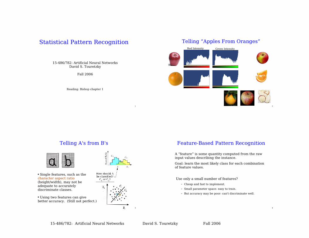
Telling �Apples From Oranges�
Red Intensity Green Intensity
3
Telling A's from B's
� Single features, such as thecharacter aspect ratio(height/width), may not beadequate to accuratelydiscriminate classes.
� Using two features can givebetter accuracy. (Still not perfect.)
4
Feature-Based Pattern Recognition
A �feature� is some quantity computed from the rawinput values describing the instance.
Goal: learn the most likely class for each combinationof feature values.
Use only a small number of features?
� Cheap and fast to implement.
� Small parameter space: easy to train.
� But accuracy may be poor: can't discriminate well.
15-486/782: Artificial Neural Networks David S. Touretzky Fall 2006
5
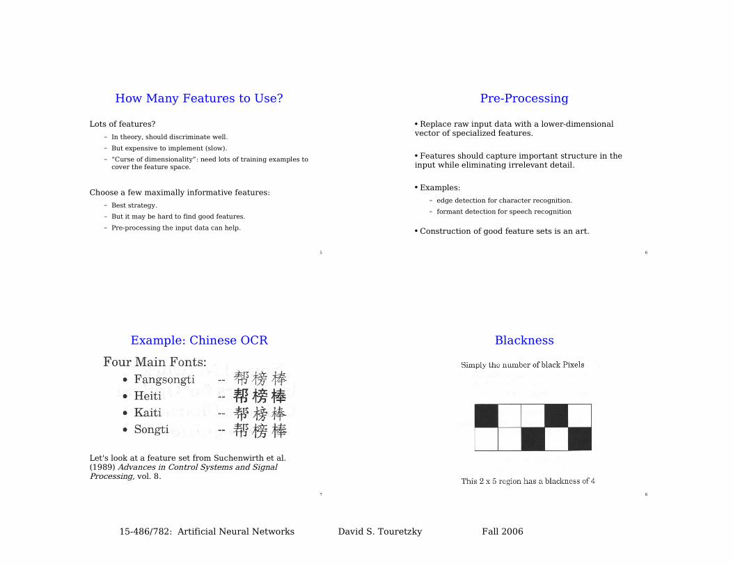
How Many Features to Use?
Lots of features?
� In theory, should discriminate well.
� But expensive to implement (slow).
� �Curse of dimensionality�: need lots of training examples tocover the feature space.
Choose a few maximally informative features:
� Best strategy.
� But it may be hard to find good features.
� Pre-processing the input data can help.
6
Pre-Processing
� Replace raw input data with a lower-dimensionalvector of specialized features.
� Features should capture important structure in theinput while eliminating irrelevant detail.
� Examples:
� edge detection for character recognition.
� formant detection for speech recognition
� Construction of good feature sets is an art.
7
Example: Chinese OCR
Let's look at a feature set from Suchenwirth et al.(1989) Advances in Control Systems and SignalProcessing, vol. 8.
8
Blackness
15-486/782: Artificial Neural Networks David S. Touretzky Fall 2006
9
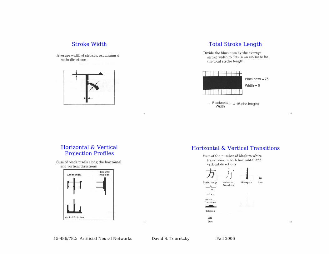
Stroke Width
10
Total Stroke Length
11
Horizontal & VerticalProjection Profiles
12
Horizontal & Vertical Transitions
15-486/782: Artificial Neural Networks David S. Touretzky Fall 2006
13
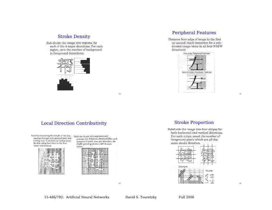
Stroke Density
14
Peripheral Features
15
Local Direction Contributivity
16
Stroke Proportion
15-486/782: Artificial Neural Networks David S. Touretzky Fall 2006
17
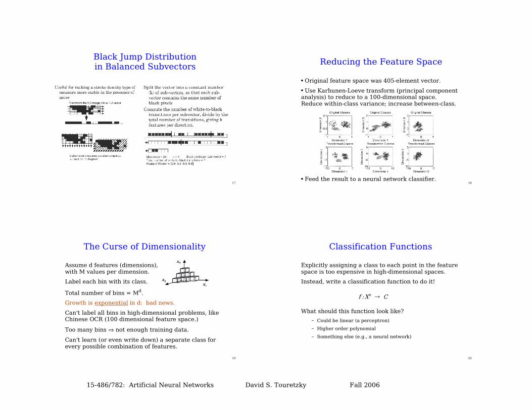
Black Jump Distributionin Balanced Subvectors
18
Reducing the Feature Space
� Original feature space was 405-element vector.
� Use Karhunen-Loeve transform (principal componentanalysis) to reduce to a 100-dimensional space.Reduce within-class variance; increase between-class.
� Feed the result to a neural network classifier.
19
The Curse of Dimensionality
Assume d features (dimensions),with M values per dimension.
Label each bin with its class.
Total number of bins = Md.
Growth is exponential in d: bad news.
Can't label all bins in high-dimensional problems, likeChinese OCR (100 dimensional feature space.)
Too many bins ⇒ not enough training data.
Can't learn (or even write down) a separate class forevery possible combination of features.
20
Classification Functions
Explicitly assigning a class to each point in the featurespace is too expensive in high-dimensional spaces.
Instead, write a classification function to do it!
What should this function look like?
� Could be linear (a perceptron)
� Higher order polynomial
� Something else (e.g., a neural network)
f :Xn� C
15-486/782: Artificial Neural Networks David S. Touretzky Fall 2006
21
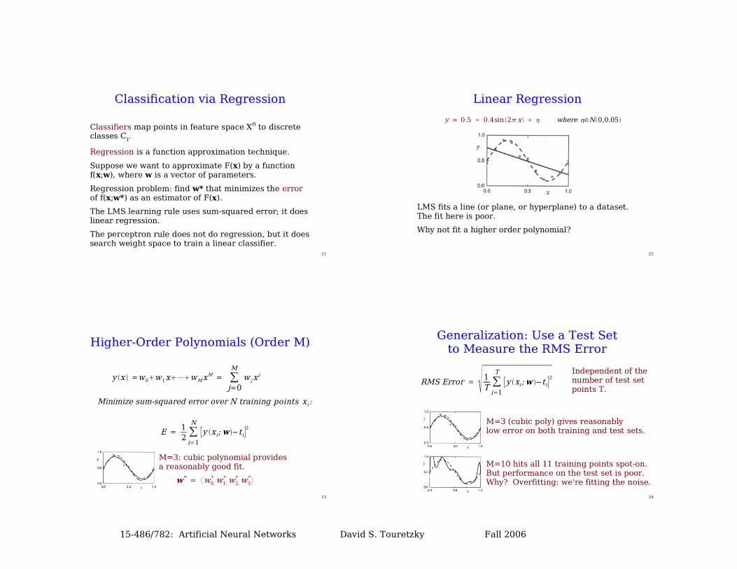
Classification via Regression
Classifiers map points in feature space Xnto discrete
classes Ci.
Regression is a function approximation technique.
Suppose we want to approximate F(x) by a functionf(x;w), where w is a vector of parameters.
Regression problem: find w* that minimizes the errorof f(x;w*) as an estimator of F(x).
The LMS learning rule uses sum-squared error; it doeslinear regression.
The perceptron rule does not do regression, but it doessearch weight space to train a linear classifier.
22
Linear Regression
y = 0.5 � 0.4sin�2�x � � � where ��N�0,0.05�
LMS fits a line (or plane, or hyperplane) to a dataset.The fit here is poor.
Why not fit a higher order polynomial?
23
Higher-Order Polynomials (Order M)
y �x � =w0�w1x��wMxM
= j=0
M
wjxj
Minimize sum-squared error over N training points xi :
E =1
2i=1
N
[y �xi;w ��ti ]2
M=3: cubic polynomial providesa reasonably good fit.
w*= �w0,
* w1,
* w2,
* w3
*
24
Generalization: Use a Test Setto Measure the RMS Error
RMS Error = �1
Ti=1
T
[y �xi ;w ��ti ]2
Independent of thenumber of test setpoints T.
M=3 (cubic poly) gives reasonablylow error on both training and test sets.
M=10 hits all 11 training points spot-on.But performance on the test set is poor.Why? Overfitting: we're fitting the noise.
15-486/782: Artificial Neural Networks David S. Touretzky Fall 2006
25
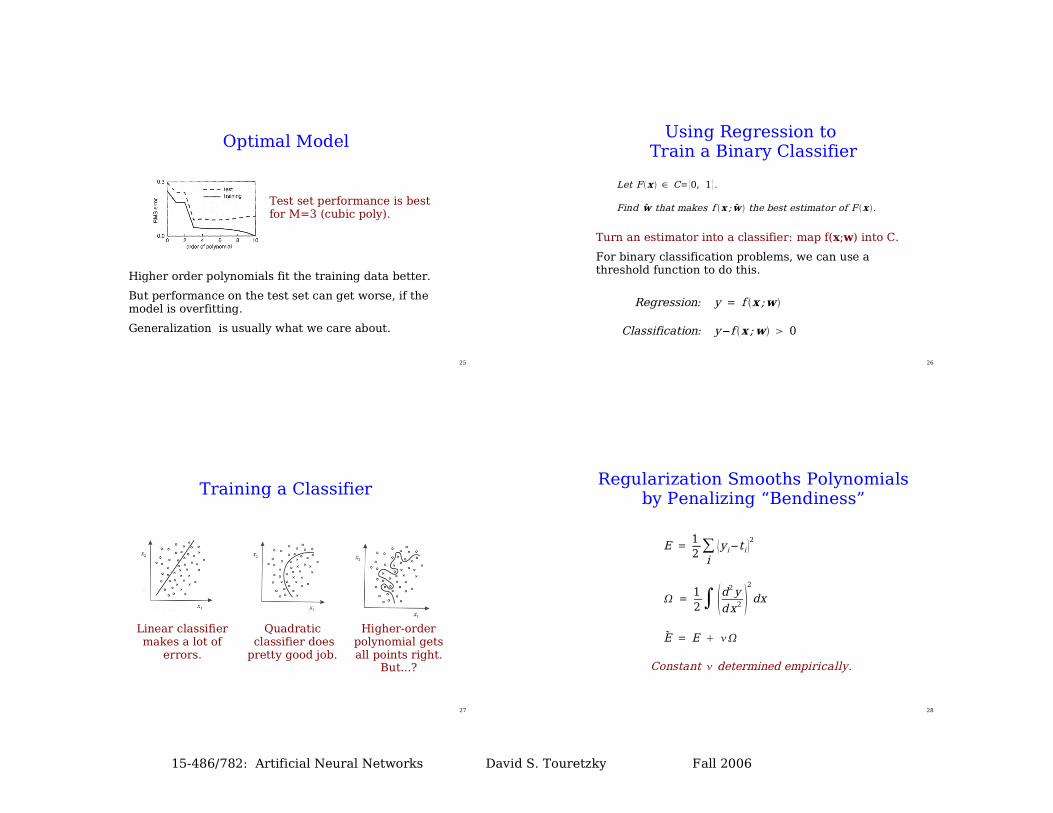
Optimal Model
Higher order polynomials fit the training data better.
But performance on the test set can get worse, if themodel is overfitting.
Generalization is usually what we care about.
Test set performance is bestfor M=3 (cubic poly).
26
Using Regression toTrain a Binary Classifier
Turn an estimator into a classifier: map f(x;w) into C.
For binary classification problems, we can use athreshold function to do this.
Let F �x � � C� {0, 1}.
Find �w that makes f �x ; �w � the best estimator of F �x �.
Regression: y = f �x ;w �
Classification: y�f �x ;w� � 0
27
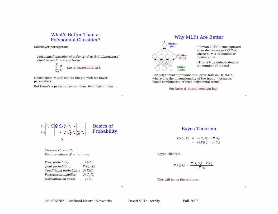
Training a Classifier
Linear classifiermakes a lot of
errors.
Quadraticclassifier doespretty good job.
Higher-orderpolynomial getsall points right.
But...?
28
Regularization Smooths Polynomialsby Penalizing �Bendiness�
E =1
2i
�yi�ti �2
� =1
2��d2y
dx2 �
2
dx
�E = E � ��
Constant � determined empirically.
15-486/782: Artificial Neural Networks David S. Touretzky Fall 2006

29
Quadratic Classifiers
Still a linear model: it's a linear function of theweights.
Think of the quadratic terms as just extra features,with weights wij.
Quadratic in n variables:
y = w0 � i=1
n
wi xi � i=1
n
j�i
n
wi xi x j
30
Building a Quadratic Classifier
Assume 2D input space: x1 and x2
y=w1�w2x1�w3x2�w4x12�w5x2
2�w6x1 x2
Decision boundary: y � 0
Training: LMS.
Shape of decision surface?parabola, hyperbola, ellipse
31
Quadratic Regression FunctionDecisionSurface
32
Plotting the Decision Boundary
x1
x2w1 � w2x1�w3x2 � w4x1
2�w5x2
2�w6x1x2 = 0
quadraticlinearconst.
w5x22� �w3�w6x1�x2 � �w1�w2x1�w4x1
2� = 0
ax22� bx2 � c = 0
x2 =�b±�b
2�4ac
2aNote: up to 2 real roots.
a b c
15-486/782: Artificial Neural Networks David S. Touretzky Fall 2006
33
What's Better Than aPolynomial Classifier?
Multilayer perceptrons!
Neural nets (MLPs) can do the job with far fewerparameters.
But there's a price to pay: nonlinearity, local minima ...
Polynomial classifier of order k�d with d-dimensionalinput needs how many terms?
i=0
kdi
i !this is exponential in k
34
Why MLPs Are Better
� Barron (1993): sum-squarederror decreases as O(1/M),where M = # of nonlinearhidden units.
� This is true independent ofthe number of inputs!
Output
Unit
Hidden
Units
Input
Units
For polynomial approximators, error falls as O(1/M2/d),where d is the dimensionality of the input. (Assumeslinear combination of fixed polynomial terms.)
For large d, neural nets win big!
35
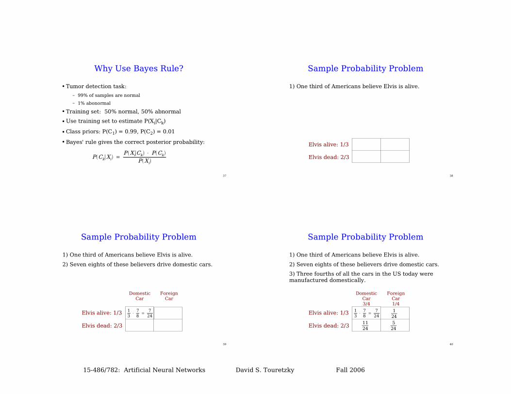
Basics ofProbability
C1
C2
X
Classes: C1 and C2
Feature values: X = {x1,,x9}
Prior probability: P�Ck�
Joint probability: P �Ck,Xl�
Conditional probability: P�Xl�Ck�
Posterior probability: P�Ck�Xl�
Normalization const. P �Xl �
36
Bayes Theorem
Bayes Theorem:
This will be on the midterm.
P�Ck, Xl� = P �Ck�Xl� � P�Xl�
= P�Xl�Ck� � P �Ck �
P�Ck�Xl� =P �Xl�Ck� � P�Ck�
P�Xl�
15-486/782: Artificial Neural Networks David S. Touretzky Fall 2006
37
Why Use Bayes Rule?
� Tumor detection task:
� 99% of samples are normal
� 1% abonormal
� Training set: 50% normal, 50% abnormal
� Use training set to estimate P(Xi|Ck)
� Class priors: P(C1) = 0.99, P(C2) = 0.01
� Bayes' rule gives the correct posterior probability:
P�Ck�Xi� =P �Xi�Ck� � P�Ck�
P�Xi�
38
Sample Probability Problem
1) One third of Americans believe Elvis is alive.
Elvis alive: 1/3
Elvis dead: 2/3
39
Sample Probability Problem
1) One third of Americans believe Elvis is alive.
2) Seven eights of these believers drive domestic cars.
DomesticCar
ForeignCar
Elvis alive: 1/3
Elvis dead: 2/3
1
3�7
8=
7
24
40
Sample Probability Problem
1) One third of Americans believe Elvis is alive.
2) Seven eights of these believers drive domestic cars.
3) Three fourths of all the cars in the US today weremanufactured domestically.
DomesticCar3/4
ForeignCar1/4
Elvis alive: 1/3
Elvis dead: 2/3
1
3�7
8=
7
24
11
24
1
24
5
24
15-486/782: Artificial Neural Networks David S. Touretzky Fall 2006
41
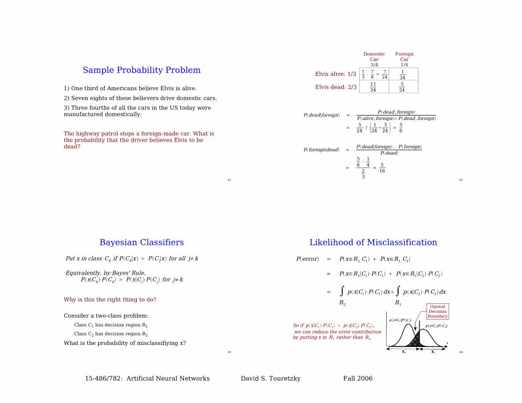
Sample Probability Problem
1) One third of Americans believe Elvis is alive.
2) Seven eights of these believers drive domestic cars.
3) Three fourths of all the cars in the US today weremanufactured domestically.
The highway patrol stops a foreign-made car. What isthe probability that the driver believes Elvis to bedead?
42
DomesticCar3/4
ForeignCar1/4
Elvis alive: 1/3
Elvis dead: 2/3
1
3�7
8=
7
24
11
24
1
24
5
24
P�foreign�dead� =P �dead�foreign� � P �foreign�
P�dead�
=
5
6�1
4
2
3
=5
16
P�dead�foreign� =P �dead,foreign�
P �alive,foreign ��P �dead,foreign�
=5
24/ �
1
24�
5
24 � =5
6
43
Bayesian Classifiers
Why is this the right thing to do?
Consider a two-class problem:
Class C1 has decision region R1
Class C2 has decision region R2
What is the probability of misclassifiying x?
Put x in class Ck if P �Ck�x � � P �Cj�x � for all j�k
Equivalently, by Bayes' Rule,P �x�Ck��P �Ck� � P �x�Cj ��P �Cj� for j�k
44
Likelihood of Misclassification
P�error� = P�x�R2,C1� � P�x�R1,C2�
= P�x�R2�C1��P�C1� � P�x�R1�C2��P�C2�
= �R2
p�x�C1��P�C1�dx��R1
p �x�C2��P�C2�dx
So if p�x�C1��P �C1� � p�x�C2��P�C2�,
we can reduce the error contributionby putting x in R1 rather than R2.
OpimalDecisionBoundary
15-486/782: Artificial Neural Networks David S. Touretzky Fall 2006
45
Good News
A properly trained neural network
will approximate
the Bayesian posterior probabilities
P(Ck | x)
46
Discriminant Functions DoPattern Classification
Define yk �x � � P �Ck�x � (discriminant function)
Could train a separate function approximator for each yk
Class of x is: argmaxk yk �x �
Decision boundary between Cj and Ck is at:
y j �x � = yk �x �
Special trick for two-class problems: define
y �x � = y1�x � � y2 �x �
Assign x to C1 if y �x ��0.
One function discriminates two classes.
15-486/782: Artificial Neural Networks David S. Touretzky Fall 2006