Statistical Predictors of March Madness: An Examination …economics-files.pomona.edu/GarySmith/Econ190/Wright... · Statistical Predictors of March Madness: ... you only pick winners

Wright 1

Statistical Predictors of March Madness:

An Examination of the NCAA Men’s’ Basketball Championship

Chris Wright

Pomona College Economics Department

April 30, 2012

Wright 2

1. Introduction

1.1 History of the Tournament

The NCAA Men’s Division I Basketball Championship, known as “March

Madness,” is one of the most popular sporting events in the United States. The

championship is a single-elimination tournament that takes place at various

locations throughout the United States each spring. The current format features 68

teams at the beginning of the tournament, but it has not always been such a large

field. Since its origins as an eight-team tournament in 1939, the NCAA has changed

and expanded the basketball championship many times. The largest changes include

1975, when the field grew to 32 teams and at-large teams1 began to be placed into

the tournament; 1985, when the field was expanded to 64 teams; and most recently

in 2011, when the tournament was changed to feature 68 teams (with four play-in

games occurring before the first round).

1.2 Qualifying and Selection

In the current format, 68 teams participate in the single-elimination

championship tournament. Of these 68 teams that qualify for the championship

tournament, 31 earn automatic bids by winning their respective conferences that

year. The remaining 37 teams are given at-large bids by the Selection Committee, a

special committee appointed by the NCAA. This committee is also responsible for

dividing the field into four regions with 16 teams each and assigning seeding within

each region. The Committee is responsible for making each region as close as

possible in terms of overall quality of teams. This means, for instance, that the 7-

1 “At-large teams” are teams that did not automatically qualify for the tournament by winning their conference tournament, but were invited by the selection committee based on their merit.

Wright 3

seeded team in one region should be very close in quality to the 7-seeded team from

any of the other three regions. The names of the regions vary each year, and are

typically based on the general geographic location of the host site of each region’s

semifinal and final matchups. For example, in 2012, the four regions were the South

(Atlanta), East (Boston), West (Phoenix, AZ), and Midwest (St. Louis).

1.3 Current Format and Rules

The current 68-team format closely resembles the 64-team tournament that

was introduced in 1985. The notable exception is the so-called “First Four” round of

play-in games2. In this round, four games are played amongst the lowest four at-

large qualifying teams and the lowest four automatic bid (i.e. conference champion)

teams, as determined by the Selection Committee. These teams are not necessarily

playing for a 16 seed; in 2012 for instance, the “First Four” consisted of matchups

for a 12 seed, a 14 seed, and two 16 seeds. Nor is there necessarily one play-in game

per region; in 2012 the Midwest region featured two play-in games and the East

featured none. After this “First Four” round is complete, there are 64 teams

remaining and the rest of the field begins play.

The tournament is typically played over the course of three weekends in

March and April. The tournament is a single-elimination tournament, thus all games

played eliminate the losing team. Over the first two weekends, the four regions of

sixteen teams are entirely separated from each other, and four regional champions

emerge after four rounds of games have been completed. These four teams then

2 This play-in round is often referred to as the first round and the round of 64 is then referred to as the second round; however, to avoid confusion between data that are from years before 2011, the round of 64 will be referred to as the “first round” in this paper.

Wright 4

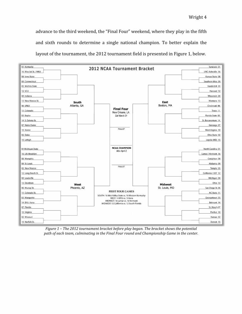
advance to the third weekend, the “Final Four” weekend, where they play in the fifth

and sixth rounds to determine a single national champion. To better explain the

layout of the tournament, the 2012 tournament field is presented in Figure 1, below.

Figure 1 – The 2012 tournament bracket before play began. The bracket shows the potential

path of each team, culminating in the Final Four round and Championship Game in the center.

Wright 5

The 64-team format always follows the example shown in Figure 1. Note how

the first round consists of the 1st seed playing against the 16th seed, the 2nd seed

playing the 15th seed, and so on. In the second round, the winner of the 1 vs. 16

matchup plays the winner of the 8 vs. 9 matchup, the 2 vs. 15 winner plays the 7 vs.

10 winner, and so on. Also notice how the winner of the West region plays the

winner of the South region, no matter which teams win from these regions.

1.4 Bracketology

For years, it has been popular to attempt to predict the correct outcomes of

all the games before the tournament starts by filling out a bracket, despite the odds

being 263 : 1 against randomly picking the entire bracket correctly (for a sixty-four

team field).3 In 2011, President Obama referred to filling out a bracket as a national

pastime and revealed his own bracket predictions on an ESPN segment. Putting

money on one’s ability to predict tournament winners is also a popular aspect to

March Madness; an estimated $7 billion is wagered annually on the outcomes of

tournament games, typically in the form of private friend pools or office pools

(Rushin, 2009). The objective of my research will be to design a model that is

successfully predictive of outcomes of matchups in the March Madness basketball

tournament.

1.5 Literature Review

Due to the popularity of the tournament and the size of the (somewhat

illegitimate) market involved in wagering on it, there has been significant research

done on March Madness before.

3 A typical bracket does not make you choose the outcomes of the “first four” games, you only pick winners from the round of 64 onwards.

Wright 6

One factor that has been studied extensively for its value as a predictor of

success is a team’s seed in the tournament, as assigned by the Selection Committee

on Selection Sunday. It has been found that seeding is a significant predictor for the

earlier rounds, but has less value in predicting outcomes of the final three rounds of

the tournament (Jacobson and King 2009). Boulier and Stekler (1999) also looked at

tournament seeds by using a probit analysis to determine the probability of teams

winning a given matchup based solely on seed and found that it was a good

predictor, especially in early rounds. Other models examined by Jacobson and King

(2009) used average win margins, Vegas lines, season wins and losses, and press

rankings to attempt to predict winners. These models have mostly been found to be

predictive in the early rounds, but less helpful for later rounds. My goal is to build a

model that uses more data for each team and can predict outcomes of the later

round games, where well studied factors such as seeding seem to matter less. The

ultimate goal is to be able to predict teams that will not only make it to the final

rounds, but also succeed when they get there.

2. Methods

2.1 Data Sample

The data that I have used for my research are historical statistics compiled

for teams from the NCAA tournament from the years 1986 - 2010. The data

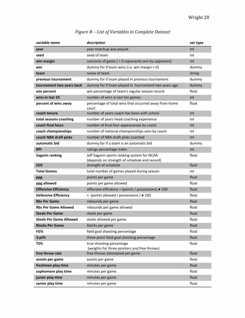
collected are made up of 74 variables for each matchup, listed in Appendix I, Figure

B. About half of the variables for each matchup refer to the given team4, and half

4 The higher seed in the matchup is designated ‘team’; the lower seed is designated ‘opponent.’ If a game is in the final two rounds, it is possible that the seeds are equal, in which case the school name that is first alphabetically is designated as ‘team.’

Wright 7

refer to the opponent (denoted as “opp_variable name”), with a few referring to the

matchup itself.

In all, I have data on the teams and outcomes from 1575 matchups over the

twenty-five year period that I am examining.5 It is important to note that I have

created the dataset so that it represents each matchup of teams rather than each

individual team isolated from their opponent. The dependent variable that I have

compiled for analysis is margin of victory for the higher seed in any given matchup,

with a negative number therefore representing a win by the lower seed. I also have

a dummy variable called “win” that takes a value of 1 if the margin of victory is

greater than zero. I obtained all the data for matchups and final scores from

databasesports.com and sportsreference.com. A spread sheet version of the dataset

can be found here.6

2.2 Data Analysis Overview

I will run a probit regression and an ordinary least squares (OLS) linear

regression. The independent variables will consist of a combination of the variables

that describe the teams in each matchup, and the dependent variable will be a

dummy for a win in the probit model, and the margin of victory in the OLS linear

regression.

3. Results

I have created two models to test with my data. One model uses variables

that are only present in the dataset from 1997 onwards, such as offensive efficiency

5 A large portion of these data were obtained from Emily Toutkoushian, a graduate of Ohio State University, who compiled a March Madness dataset in 2011 for her own research at OSU into predicting March Madness. 6 https://docs.google.com/spreadsheet/ccc?key=0Aq4oJhIoBJm1dFp3U3JyVFp4aDNRTlpCcXRNQjFUSnc

Wright 8

and defensive efficiency, as well as variables that are present in the entire dataset,

from 1986 onwards. The other model contains only variables that are present

throughout the entire time period and thus can be estimated and tested across the

entire sample.

3.1 Model One

Model One uses some variables that are only present in the dataset from

1997 onwards, meaning for this model we can only utilize about half of the total

range of years. My second will use data from the entire time period, but I felt that

some of the variables only present in recent data were important to consider, hence

I have created Model One. The variables to be used as input in Model One are as

follows:

seed

win percent

wins in last ten

Sagarin rank

ppg

ppg allowed

offensive efficiency*

defensive efficiency*

true shooting percentage*

assists per game*

coach final fours*

percent of wins away

opp_seed

opp_win percent

opp_wins in last ten

opp_Sagarin ranking

opp_ppg

opp_ppg allowed

opp_offensive efficiency*

opp_defensive efficiency*

opp_true shooting percentage*

opp_assists per game*

opp_coach final fours*

opp_percent of wins away

* refers to variables only collected from 1997 onwards

Wright 9

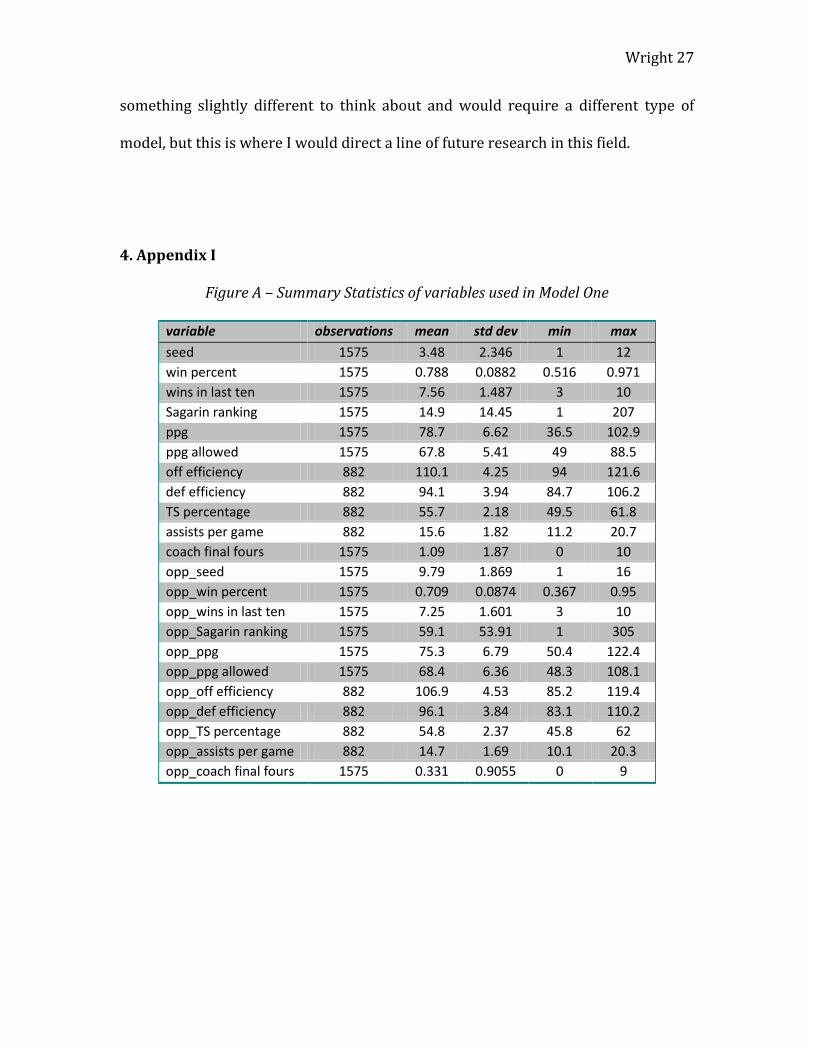
I have decided upon these variables as they are intuitively important inputs that

I consider when I am choosing my own bracket. Summary statistics describing these

variables are presented in Appendix I, Figure A.

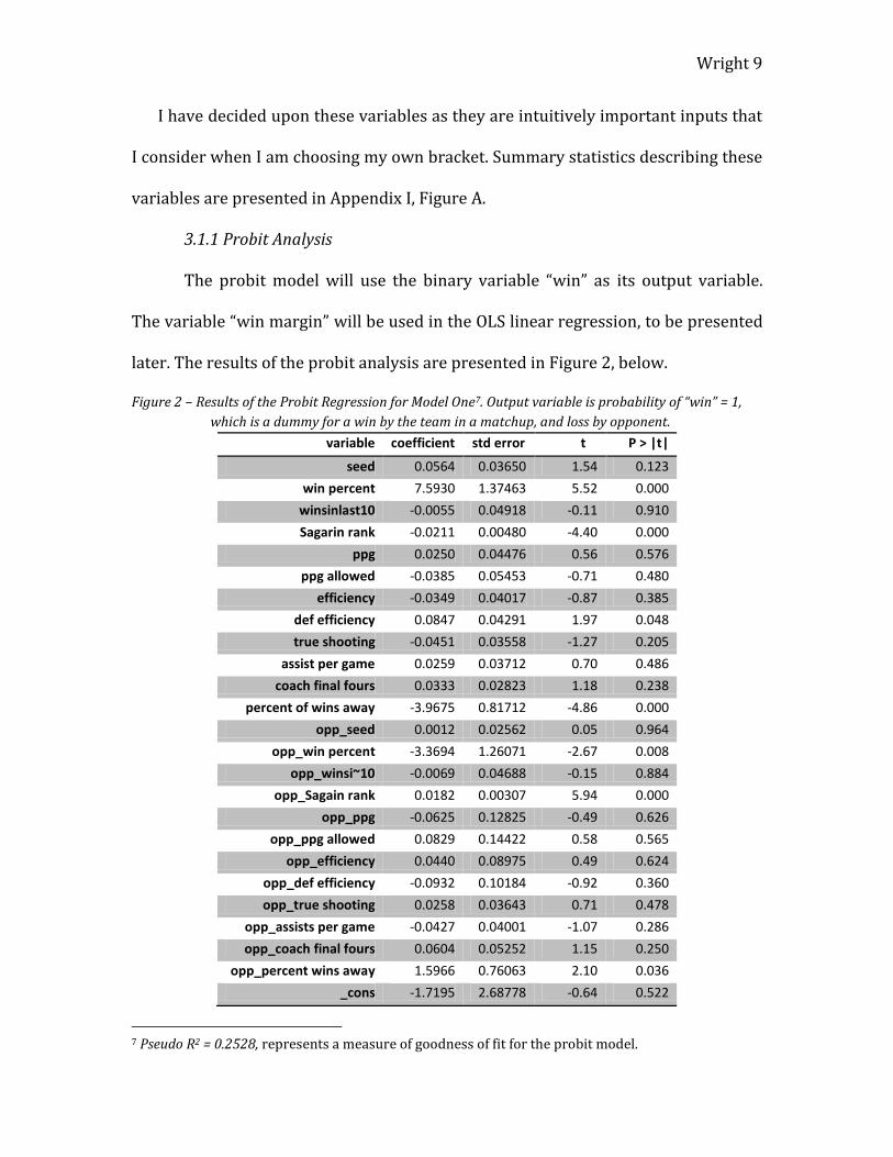
3.1.1 Probit Analysis

The probit model will use the binary variable “win” as its output variable.

The variable “win margin” will be used in the OLS linear regression, to be presented

later. The results of the probit analysis are presented in Figure 2, below.

Figure 2 – Results of the Probit Regression for Model One7. Output variable is probability of “win” = 1,

which is a dummy for a win by the team in a matchup, and loss by opponent.

variable coefficient std error t P > |t|

seed 0.0564 0.03650 1.54 0.123

win percent 7.5930 1.37463 5.52 0.000

winsinlast10 -0.0055 0.04918 -0.11 0.910

Sagarin rank -0.0211 0.00480 -4.40 0.000

ppg 0.0250 0.04476 0.56 0.576

ppg allowed -0.0385 0.05453 -0.71 0.480

efficiency -0.0349 0.04017 -0.87 0.385

def efficiency 0.0847 0.04291 1.97 0.048

true shooting -0.0451 0.03558 -1.27 0.205

assist per game 0.0259 0.03712 0.70 0.486

coach final fours 0.0333 0.02823 1.18 0.238

percent of wins away -3.9675 0.81712 -4.86 0.000

opp_seed 0.0012 0.02562 0.05 0.964

opp_win percent -3.3694 1.26071 -2.67 0.008

opp_winsi~10 -0.0069 0.04688 -0.15 0.884

opp_Sagain rank 0.0182 0.00307 5.94 0.000

opp_ppg -0.0625 0.12825 -0.49 0.626

opp_ppg allowed 0.0829 0.14422 0.58 0.565

opp_efficiency 0.0440 0.08975 0.49 0.624

opp_def efficiency -0.0932 0.10184 -0.92 0.360

opp_true shooting 0.0258 0.03643 0.71 0.478

opp_assists per game -0.0427 0.04001 -1.07 0.286

opp_coach final fours 0.0604 0.05252 1.15 0.250

opp_percent wins away 1.5966 0.76063 2.10 0.036

_cons -1.7195 2.68778 -0.64 0.522

7 Pseudo R2 = 0.2528, represents a measure of goodness of fit for the probit model.

Wright 10

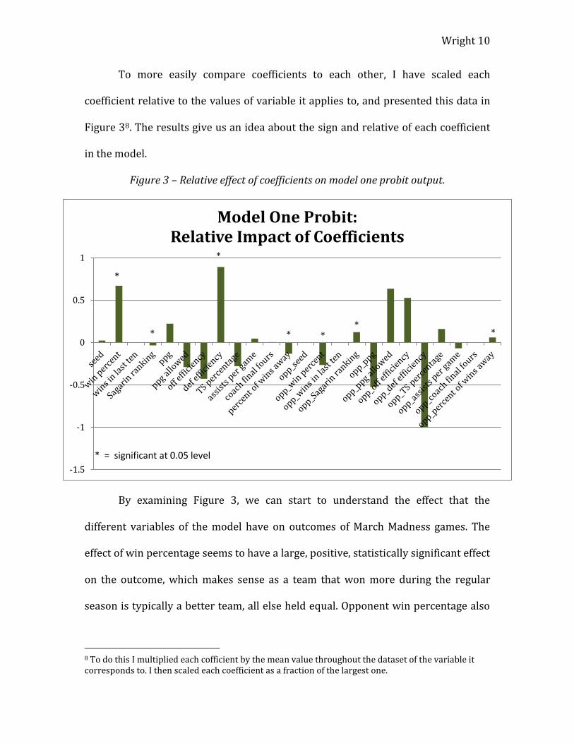
To more easily compare coefficients to each other, I have scaled each

coefficient relative to the values of variable it applies to, and presented this data in

Figure 38. The results give us an idea about the sign and relative of each coefficient

in the model.

Figure 3 – Relative effect of coefficients on model one probit output.

By examining Figure 3, we can start to understand the effect that the

different variables of the model have on outcomes of March Madness games. The

effect of win percentage seems to have a large, positive, statistically significant effect

on the outcome, which makes sense as a team that won more during the regular

season is typically a better team, all else held equal. Opponent win percentage also

8 To do this I multiplied each cofficient by the mean value throughout the dataset of the variable it corresponds to. I then scaled each coefficient as a fraction of the largest one.

-1.5

-1

-0.5

0

0.5

1

Model One Probit: Relative Impact of Coefficients

*

*

*

* * *

*

* = significant at 0.05 level

Wright 11

has an effect, not as large as a team’s own win percentage, but in the opposite

direction, which also makes intuitive sense.

Sagarin rankings also seem to have a statistically significant effect on the

outcomes of games. A team’s Sagaring rank has a negative effect on the outcome of

“win,” which makes sense as better ranked teams will have lower value for their

Sagarin ranking.9 We also see that an opponent’s Sagarin ranking has a significant

positive effect on the team’s chances of a win, which also makes logical sense.

Sagarin rankings come from Jeff Sagarin, an American sports statistician well

known for his ranking systems in sports such as basketball and football. His

rankings have been featured in USA Today’s sports section since 1985.

Other variables that seemed to have a large magnitude of effect on the

probability of a win are points per game (ppg) and points per game allowed, as well

as opponent’s ppg and opponent’s ppg allowed. The effects of these variables were

not statistically significant, but the effects are in the expected direction for all four:

positive for ppg, negative for ppg allowed, negative for opp_ppg, and positive for

opp_ppg allowed.

Some unexpected effects that appear large, albeit not statistically significant,

can be seen in the efficiency variables. Each of these is affecting the outcome in the

opposite manner that would be expected. My thought here is that perhaps there is

endogeneity between the ppg variables and the efficiency variables, causing the

coefficients to be thrown off.

9 Sagarin ranking values work as follows: the “best team” is given the ranking of 1 and values go up form there. Thus a larger value for Sagarin ranking implies a worse team by Sagarin’s method.

Wright 12

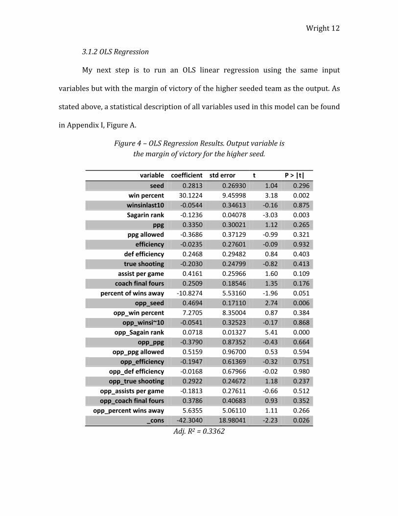
3.1.2 OLS Regression

My next step is to run an OLS linear regression using the same input

variables but with the margin of victory of the higher seeded team as the output. As

stated above, a statistical description of all variables used in this model can be found

in Appendix I, Figure A.

Figure 4 – OLS Regression Results. Output variable is

the margin of victory for the higher seed.


seed 0.2813 0.26930 1.04 0.296

win percent 30.1224 9.45998 3.18 0.002

winsinlast10 -0.0544 0.34613 -0.16 0.875

Sagarin rank -0.1236 0.04078 -3.03 0.003

ppg 0.3350 0.30021 1.12 0.265

ppg allowed -0.3686 0.37129 -0.99 0.321

efficiency -0.0235 0.27601 -0.09 0.932

def efficiency 0.2468 0.29482 0.84 0.403

true shooting -0.2030 0.24799 -0.82 0.413

assist per game 0.4161 0.25966 1.60 0.109

coach final fours 0.2509 0.18546 1.35 0.176


opp_seed 0.4694 0.17110 2.74 0.006

opp_win percent 7.2705 8.35004 0.87 0.384

opp_winsi~10 -0.0541 0.32523 -0.17 0.868

opp_Sagain rank 0.0718 0.01327 5.41 0.000

opp_ppg -0.3790 0.87352 -0.43 0.664

opp_ppg allowed 0.5159 0.96700 0.53 0.594

opp_efficiency -0.1947 0.61369 -0.32 0.751

opp_def efficiency -0.0168 0.67966 -0.02 0.980

opp_true shooting 0.2922 0.24672 1.18 0.237

opp_assists per game -0.1813 0.27611 -0.66 0.512

opp_coach final fours 0.3786 0.40683 0.93 0.352

opp_percent wins away 5.6355 5.06110 1.11 0.266

_cons -42.3040 18.98041 -2.23 0.026

Adj. R2 = 0.3362

Wright 13

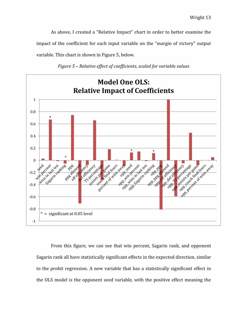
As above, I created a “Relative Impact” chart in order to better examine the

impact of the coefficient for each input variable on the “margin of victory” output

variable. This chart is shown in Figure 5, below.

Figure 5 – Relative effect of coefficients, scaled for variable values

From this figure, we can see that win percent, Sagarin rank, and opponent

Sagarin rank all have statistically significant effects in the expected direction, similar

to the probit regression. A new variable that has a statistically significant effect in

the OLS model is the opponent seed variable, with the positive effect meaning the

-1

-0.8

-0.6

-0.4

-0.2

0

0.2

0.4

0.6

0.8

1

Model One OLS: Relative Impact of Coefficients

*

*

* *


Wright 14

greater value an opponent’s seed (i.e. worse seed), the greater the expected margin

of victory in a matchup, all else held equal. This is the effect that one would

intuitively expect from this input variable.

In another similarity to the probit model, the four “point per game” input

variables10 all have effects of a large magnitude in the expected directions, but are

not statistically significant. The efficiency variables are still having effects that are

counterintuitive, although of smaller magnitude in this model when compared to the

probit model.

3.2 Model Two

Model Two contains only variables that are present across all 25 years of the

dataset, allowing us to use the entire dataset in our regressions. I once again chose

input variables that I believe intuitively to be important to success of teams in

March Madness. The input variables to be used in Model Two are as follows:

● seed

● opp_seed

● win percent

● opp_win percent

● wins in last ten

● opp_wins in last ten

● percent of wins away

● opp_percent of wins away

● Sagarin rank

● opp_Sagarin rank

● Ppg

● opp_ppg

● ppg allowed ● opp_ppg allowed

10 The four are ppg, ppg allowed, opp_ppg, and opp_ppg allowed.

Wright 15

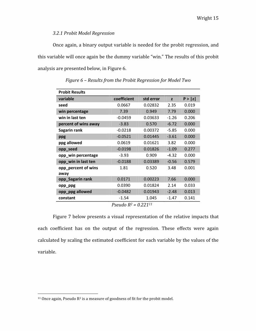
3.2.1 Probit Model Regression

Once again, a binary output variable is needed for the probit regression, and

this variable will once again be the dummy variable “win.” The results of this probit

analysis are presented below, in Figure 6.

Figure 6 – Results from the Probit Regression for Model Two

Probit Results

variable coefficient std error z P > |z|

seed 0.0667 0.02832 2.35 0.019

win percentage 7.39 0.949 7.79 0.000

win in last ten -0.0459 0.03633 -1.26 0.206


Sagarin rank -0.0218 0.00372 -5.85 0.000

ppg -0.0521 0.01445 -3.61 0.000

ppg allowed 0.0619 0.01621 3.82 0.000

opp_seed -0.0198 0.01826 -1.09 0.277

opp_win percentage -3.93 0.909 -4.32 0.000

opp_win in last ten -0.0188 0.03389 -0.56 0.579


1.81 0.520 3.48 0.001

opp_Sagarin rank 0.0171 0.00223 7.66 0.000

opp_ppg 0.0390 0.01824 2.14 0.033

opp_ppg allowed -0.0482 0.01943 -2.48 0.013

constant -1.54 1.045 -1.47 0.141

Pseudo R2 = 0.22111

Figure 7 below presents a visual representation of the relative impacts that

each coefficient has on the output of the regression. These effects were again

calculated by scaling the estimated coefficient for each variable by the values of the

variable.

11 Once again, Pseudo R2 is a measure of goodness of fit for the probit model.

Wright 16

Figure 7 – Relative impacts of coefficients, scaled for input variables values.

From Figure 7, we can examine the average effects that each variable in

Model Two had on the probit output. We can see that win percentage and opponent

win percentage have large, statistically significant effects in the direction that is

expected: positive for a given team’s win percentage and negative for an opponents

win percentage. Sagarin rank and opponents Sagarin rank also have statistically

significant effects with the expected sign. The number of statistically significant

coefficients has increased from Model One, and this could possibly be sue to the

larger sample size employed by Model Two.

One strange observation is that the points per games variables seem to have

significant effects in the directions opposite that which would be expected. That is to

-1

-0.8

-0.6

-0.4

-0.2

0

0.2

0.4

0.6

0.8

1

Model Two Probit: Relative Impact of Coefficients

*

*

* * *

*

* *

*

*

*


Wright 17

say, having outscored your opponents throughout the regular season seems to hurt

a team’s chances of winning, while playing an opponent who has outscored their

opponents throughout the season seems to help a team’s chances of winning. These

results do not make sense intuitively and my first thought is some sort of

endogeneity with other variables in the model. The percent of wins away variable

seems to affect the output in the following manner: the higher percentage of wins

that come away from a team’s home court, the lower their chances of winning a

tournament matchup, which seems counterintuitive to the mainstream thought.

3.2.2 OLS Linear Regression

The output variable in this regression will be the variable of margin of

victory. The results of the OLS regression for Model Two are presented below, in

Figure 8.

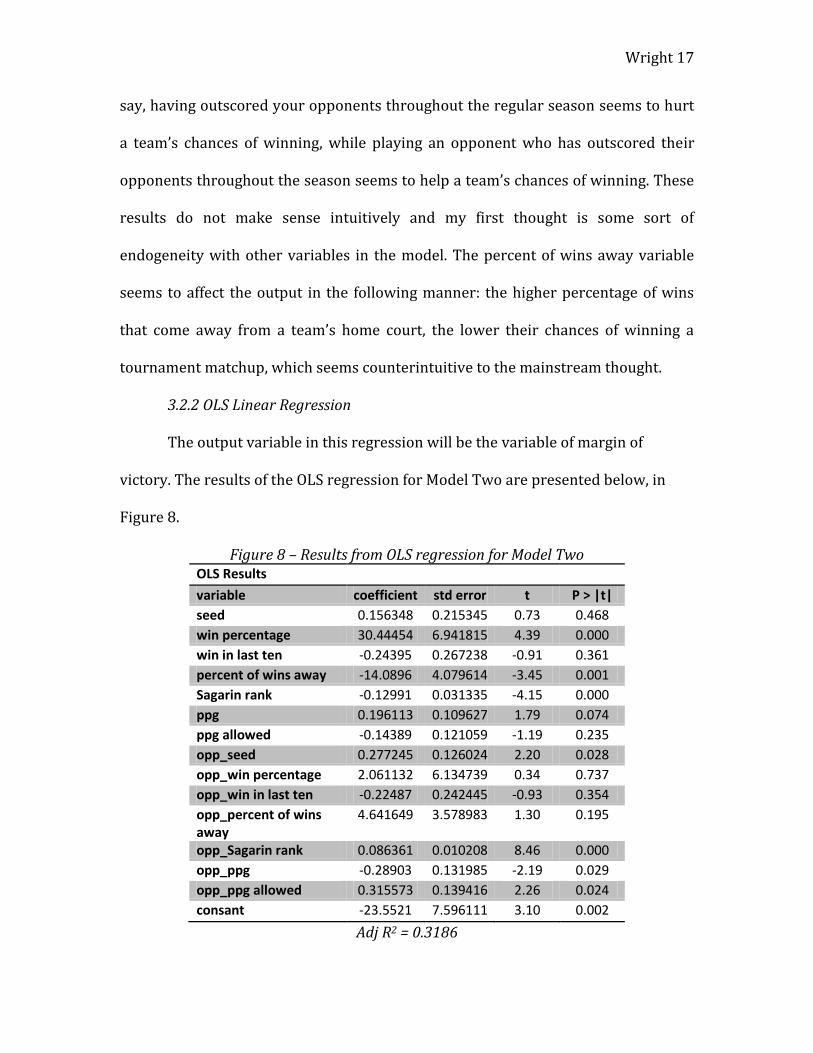
Figure 8 – Results from OLS regression for Model Two OLS Results


seed 0.156348 0.215345 0.73 0.468

win percentage 30.44454 6.941815 4.39 0.000

win in last ten -0.24395 0.267238 -0.91 0.361


Sagarin rank -0.12991 0.031335 -4.15 0.000

ppg 0.196113 0.109627 1.79 0.074

ppg allowed -0.14389 0.121059 -1.19 0.235

opp_seed 0.277245 0.126024 2.20 0.028

opp_win percentage 2.061132 6.134739 0.34 0.737

opp_win in last ten -0.22487 0.242445 -0.93 0.354


4.641649 3.578983 1.30 0.195

opp_Sagarin rank 0.086361 0.010208 8.46 0.000

opp_ppg -0.28903 0.131985 -2.19 0.029

opp_ppg allowed 0.315573 0.139416 2.26 0.024

consant -23.5521 7.596111 3.10 0.002

Adj R2 = 0.3186

Wright 18

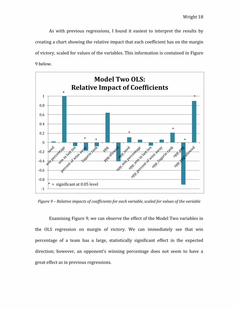
As with previous regressions, I found it easiest to interpret the results by

creating a chart showing the relative impact that each coefficient has on the margin

of victory, scaled for values of the variables. This information is contained in Figure

9 below.

Figure 9 – Relative impacts of coefficients for each variable, scaled for values of the variable

Examining Figure 9, we can observe the effect of the Model Two variables in

the OLS regression on margin of victory. We can immediately see that win

percentage of a team has a large, statistically significant effect in the expected

direction; however, an opponent’s winning percentage does not seem to have a

great effect as in previous regressions.

-1

-0.8

-0.6

-0.4

-0.2

0

0.2

0.4

0.6

0.8

1

Model Two OLS: Relative Impact of Coefficients

*

* *

* *

*

*


Wright 19

The Sagarin ranking of a team still has a statistically significant effect of the

expected sign, and the team scoring variables (ppg, ppg allowed, opponent ppg and

opponent’s ppg allowed) each have effects in the expected directions, but they are

not statistically significant. We also see the positive effect of an opponent’s seed,

which is expected as opponents with large seed values (e.g. 16 seed) represent

teams and would be expected to fare worse in a given matchup.

3.3 Predictive Abilities of Models for 2012 Tournament

To test the predictive abilities of the models constructed, I used them to

attempt to predict results from this year’s March Madness tournament before play

began, and then examined their performance after the tournament was played. The

results are on the following pages. I used ESPN’s scoring method of brackets to

evaluate the success of my models12. One model, the OLS Regression on Model One,

performed poorly and finished in the 37th percentile nationally based on ESPN’s

bracket database. The other three models all performed well, finishing at least in the

84th percentile, while the best, the Model Two OLS Regression finished with a 68.3%

accuracy of picks and scored in the 91st percentile of brackets. One thing that all

three successful brackets had in common was that they picked the number-one-

overall seed Kentucky to win the tournament, which it did. In bracket scoring,

picking the correct champion is very important, and these three models may have

performed artificially well because they were able to do this.13

12 ESPN gives 10 points for a correct first round pick, 20 points, for a correct second round pick, 40 points for a correct third round pick, and so on, up until 320 points for a correct national champion. 13 Likewise, my unsuccessful model may have done poorly because it picked St. Louis, an 8 seed from the West region, to win the championship. This seems poor to me, but may have been based on St. Louis’ scoring defense which held opponents to a very low amount of points over the season.

Wright 20

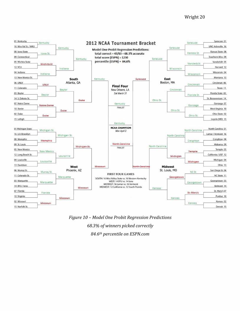
Figure 10 – Model One Probit Regression Predictions

68.3% of winners picked correctly

84.6th percentile on ESPN.com

Wright 21

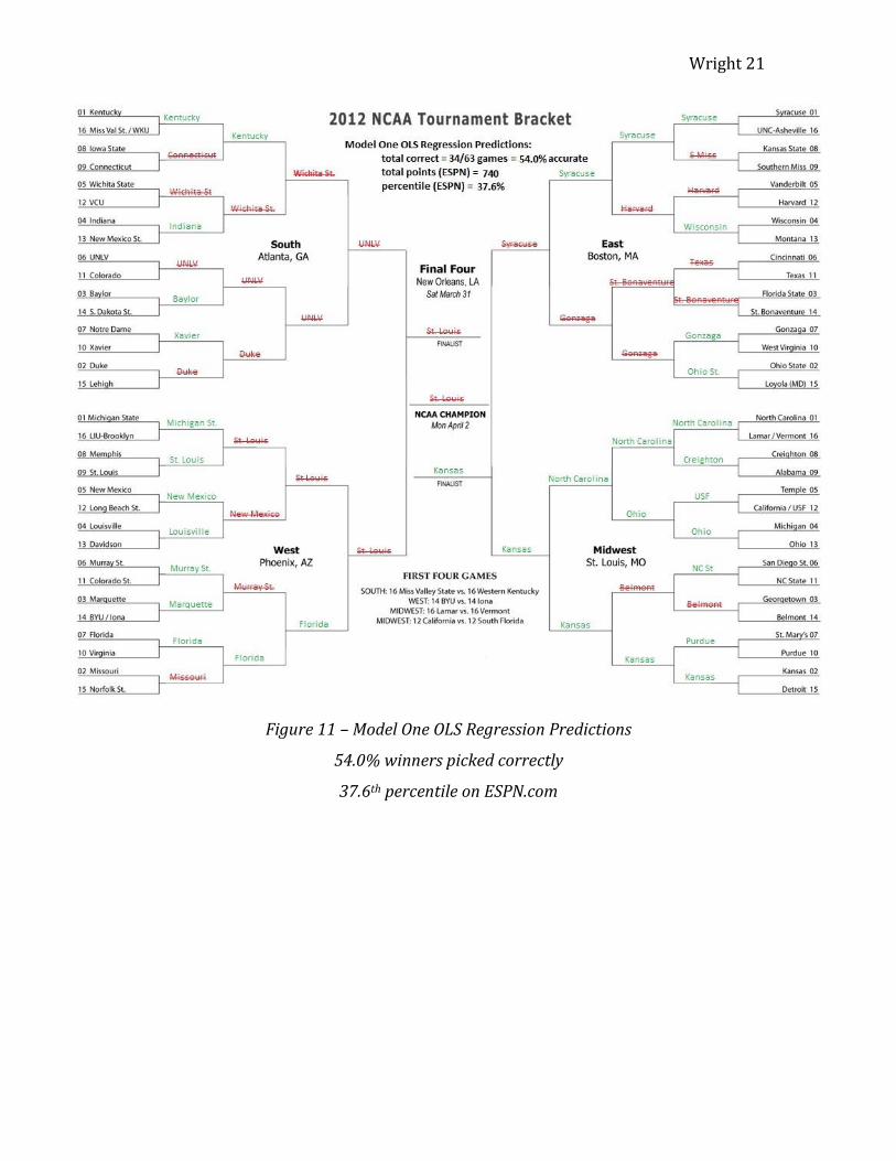
Figure 11 – Model One OLS Regression Predictions

54.0% winners picked correctly

37.6th percentile on ESPN.com

Wright 22

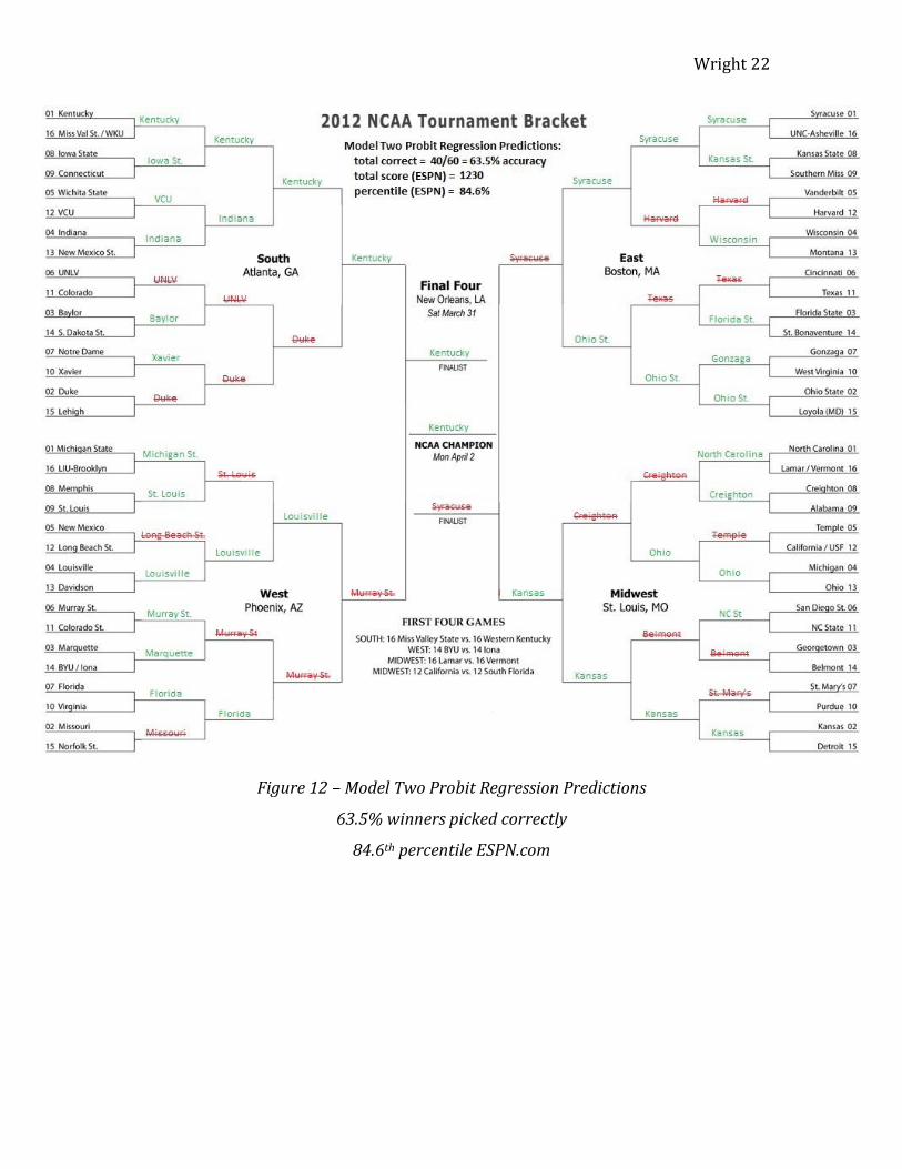
Figure 12 – Model Two Probit Regression Predictions


84.6th percentile ESPN.com

Wright 23

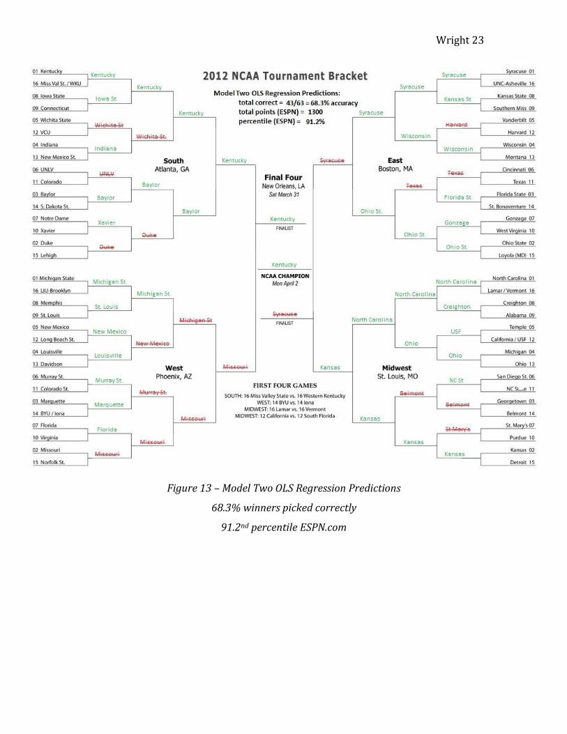
Figure 13 – Model Two OLS Regression Predictions


91.2nd percentile ESPN.com

Wright 24

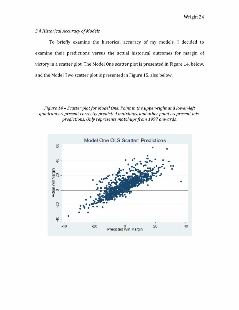
3.4 Historical Accuracy of Models

To briefly examine the historical accuracy of my models, I decided to

examine their predictions versus the actual historical outcomes for margin of

victory in a scatter plot. The Model One scatter plot is presented in Figure 14, below,

and the Model Two scatter plot is presented in Figure 15, also below.

Figure 14 – Scatter plot for Model One. Point in the upper-right and lower-left quadrants represent correctly predicted matchups, and other points represent mis-

predictions. Only represents matchups from 1997 onwards.

Wright 25

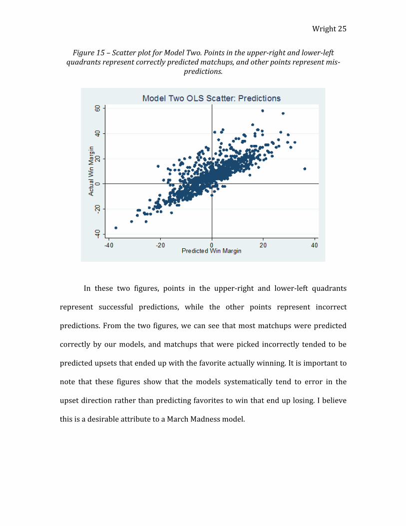
Figure 15 – Scatter plot for Model Two. Points in the upper-right and lower-left quadrants represent correctly predicted matchups, and other points represent mis-

predictions.

In these two figures, points in the upper-right and lower-left quadrants

represent successful predictions, while the other points represent incorrect

predictions. From the two figures, we can see that most matchups were predicted

correctly by our models, and matchups that were picked incorrectly tended to be

predicted upsets that ended up with the favorite actually winning. It is important to

note that these figures show that the models systematically tend to error in the

upset direction rather than predicting favorites to win that end up losing. I believe

this is a desirable attribute to a March Madness model.

Wright 26

4. Conclusion

Overall, it seems like it is very difficult to predict the winners of March

Madness matchups. Even if an unbiased model for predicting outcomes of games

could be constructed, I would expect that the error term is large enough to create a

lot of outcomes that were not predicted. In light of this, I am pretty impressed with

the performance of three of my four models. More review is needed to cross validate

my models across my historical data; however, for the 2012 tournament, these three

models performed quite successfully ‒ all of them beat the bracket that I picked by

hand myself this year.

The model that did not perform well, the OLS Regression for Model One,

seemed to pick an unreasonable amount of upsets, including selecting a Final Four

containing a six seed in UNLV and an eight seed in St. Louis. I am not sure why this

model was so prone to picking upsets, but one possibility is that it heavily weighted

the amount of points that opponents gave up during the regular season. For some

small schools that play in less skilled conferences, games typically are lower scoring

due to a generally lower level of offensive talent and slower paced games. This could

result in schools that are defensive oriented and in small conferences, such as St.

Louis, to be more favored by the model.

In the end, I believe that it is very difficult to consistently do well in picking

brackets for March Madness. Rather than attempting to pick all 63 games correctly,

the task that may be more useful to focus on in the future is picking the overall

champion, as this is worth by far the most points of any matchup. This would be

Wright 27

something slightly different to think about and would require a different type of

model, but this is where I would direct a line of future research in this field.

4. Appendix I

Figure A – Summary Statistics of variables used in Model One

variable observations mean std dev min max

seed 1575 3.48 2.346 1 12

win percent 1575 0.788 0.0882 0.516 0.971

wins in last ten 1575 7.56 1.487 3 10

Sagarin ranking 1575 14.9 14.45 1 207

ppg 1575 78.7 6.62 36.5 102.9

ppg allowed 1575 67.8 5.41 49 88.5

off efficiency 882 110.1 4.25 94 121.6

def efficiency 882 94.1 3.94 84.7 106.2

TS percentage 882 55.7 2.18 49.5 61.8

assists per game 882 15.6 1.82 11.2 20.7

coach final fours 1575 1.09 1.87 0 10

opp_seed 1575 9.79 1.869 1 16

opp_win percent 1575 0.709 0.0874 0.367 0.95

opp_wins in last ten 1575 7.25 1.601 3 10

opp_Sagarin ranking 1575 59.1 53.91 1 305

opp_ppg 1575 75.3 6.79 50.4 122.4

opp_ppg allowed 1575 68.4 6.36 48.3 108.1

opp_off efficiency 882 106.9 4.53 85.2 119.4

opp_def efficiency 882 96.1 3.84 83.1 110.2

opp_TS percentage 882 54.8 2.37 45.8 62

opp_assists per game 882 14.7 1.69 10.1 20.3

opp_coach final fours 1575 0.331 0.9055 0 9

Wright 28

Figure B – List of Variables in Complete Dataset

variable name description var type

year year matchup was played int

seed seed of team int

win margin outcome of game ( < 0 represents win by opponent) int

win dummy for if team wins (i.e. win margin > 0) dummy

team name of team string

previous tournament dummy for if team played in previous tournament dummy

tournament two years back dummy for if team played in tournament two years ago dummy

win percent win percentage of team's regular season record float

wins in last 10 number of wins in last ten games int

percent of wins away percentage of total wins that occurred away from home court

float

coach tenure number of years coach has been with school int

total seasons coaching number of years head coaching experience int

coach final fours number of final four appearances by coach int

coach championships number of national championships won by coach int

coach NBA draft picks number of NBA draft picks coached int

automatic bid dummy for if a team is an automatic bid dummy

RPI ratings percentage index int

Sagarin ranking Jeff Sagarin sports ranking system for NCAA (depends on strength of schedule and record)

float

SOS strength of schedule float

Total Games total number of games played during season int

ppg points per game float

ppg allowed points per game allowed float

Offensive Efficiency offensive efficiency = (points / possessions) ● 100 float

Defensive Efficiency = (points allowed / possessions ) ● 100 float

Rbs Per Game rebounds per game float

Rbs Per Game Allowed rebounds per game allowed float

Steals Per Game steals per game float

Steals Per Game Allowed steals allowed per game float

Blocks Per Game blocks per game float

FG% field goal shooting percentage float

3-pt% three point field goal shooting percentage float

TS% true shooting percentage (weights for three pointers and free throws)

float

free throw rate free throws attempted per game float

assists per game assists per game float

freshmen play time minutes per game float

sophomore play time minutes per game float

junior play time minutes per game float

senior play time minutes per game float

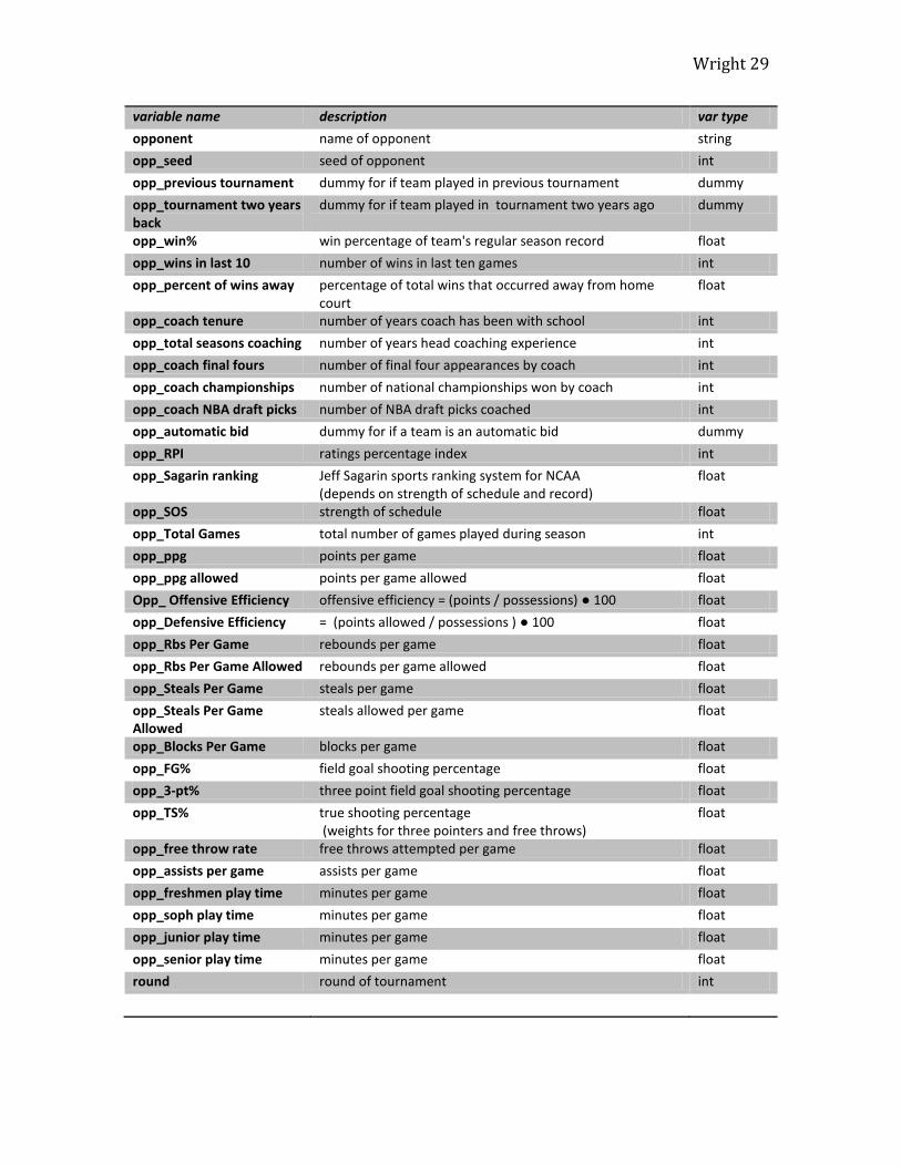
Wright 29

variable name description var type

opponent name of opponent string

opp_seed seed of opponent int

opp_previous tournament dummy for if team played in previous tournament dummy

opp_tournament two years back

dummy for if team played in tournament two years ago dummy

opp_win% win percentage of team's regular season record float

opp_wins in last 10 number of wins in last ten games int

opp_percent of wins away percentage of total wins that occurred away from home court

float

opp_coach tenure number of years coach has been with school int

opp_total seasons coaching number of years head coaching experience int

opp_coach final fours number of final four appearances by coach int

opp_coach championships number of national championships won by coach int

opp_coach NBA draft picks number of NBA draft picks coached int

opp_automatic bid dummy for if a team is an automatic bid dummy

opp_RPI ratings percentage index int

opp_Sagarin ranking Jeff Sagarin sports ranking system for NCAA (depends on strength of schedule and record)

float

opp_SOS strength of schedule float

opp_Total Games total number of games played during season int

opp_ppg points per game float

opp_ppg allowed points per game allowed float

Opp_ Offensive Efficiency offensive efficiency = (points / possessions) ● 100 float

opp_Defensive Efficiency = (points allowed / possessions ) ● 100 float

opp_Rbs Per Game rebounds per game float

opp_Rbs Per Game Allowed rebounds per game allowed float

opp_Steals Per Game steals per game float

opp_Steals Per Game Allowed

steals allowed per game float

opp_Blocks Per Game blocks per game float

opp_FG% field goal shooting percentage float

opp_3-pt% three point field goal shooting percentage float

opp_TS% true shooting percentage (weights for three pointers and free throws)

float

opp_free throw rate free throws attempted per game float

opp_assists per game assists per game float

opp_freshmen play time minutes per game float

opp_soph play time minutes per game float

opp_junior play time minutes per game float

opp_senior play time minutes per game float

round round of tournament int

Wright 30

5. References

Boulier, B. and Stekler, H. (1999). Are Sports Seedings Good Predictor?: an

evaluation. International Journal of Forecasting, 1999, 15 83-91.

Jacobson, S. and King, D. (2009). Seeding in the NCAA Men’s Basketball

Tournament: when is a higher seed better?

https://netfiles.uiuc.edu/shj/www/JK_NCAAMM.pdf

Metrick, A. (1996). March Madness? Strategic behavior in NCAA basketball

tournament betting pools. Journal of Economic Behavior & Organization,

1996, 30, 159-172.

McClure, J. and Spector, L. Tournament Performance and Agency Problems: An

empirical investigation of “March Madness.” Journal of Economics and

Finance 21(1), 61-68.

Rushin, S. (2009). The Bracket Racket. ESPN college basketball encyclopedia,

Ballantine Books, New York, NY.

www.espn.com

www.sportsreference.com

Sagarin, J. (2012) Jeff Sagarin NCAA Basketball Ratings. USA Today.com/sports

Schwertman, N. Schenk K, Holbrook, B. More Probability Models for the NCAA

Regional Basketball Tournaments. The American Statistician (1996) 50(1),

pg. 3438

Bryan, K. Steinke, M. Wilkins, N. Upset Special: Are March Madness Upsets

Predictable? (April 28, 2006). http://ssrn.com/abstract=899702

https://netfiles.uiuc.edu/shj/www/JK_NCAAMM.pdf

http://www.espn.com/

http://www.sportsreference.com/

Documents

Statistical Predictors of March Madness: An Examination …economics-files.pomona.edu/GarySmith/Econ190/Wright... · Statistical Predictors of March Madness: ... you only pick winners