Embed Size (px)
Citation preview

STATISTICAL TECHNIQUES FOR BIOLOGICAL
MOTIF DISCOVERY
A Dissertation
Presented to the Faculty of the Graduate School
of Cornell University
in Partial Fulfillment of the Requirements for the Degree of
Doctor of Philosophy
by
Niranjan Nagarajan
January 2007

c© 2007 Niranjan Nagarajan
ALL RIGHTS RESERVED

STATISTICAL TECHNIQUES FOR BIOLOGICAL MOTIF DISCOVERY
Niranjan Nagarajan, Ph.D.
Cornell University 2007
In recent years, the various genome sequencing projects and computational and
experimental efforts to find genes have provided us with a wealth of sequence
information in protein and DNA databases. A large portion of this sequence data
is however yet to be characterized. Experimental efforts and manual curation have
tried to keep up with the flood of data, but it has become increasingly clear that
reliable computational methods are required to fill in the gap. In addition to its
value in furthering research in basic biology, improved computational tools for
annotating Proteomes and Genomes serve as an important first step in realizing
the biomedical promise of whole-cell modelling and systems biology.
In this dissertation we discuss statistical and algorithmic techniques for two
important areas in the field of biological sequence analysis. We begin by discussing
our work on improving a class of motif finding tools that are widely used to discover
regulatory signals in DNA. This work is based on new ideas in computational
statistics that provide us with efficient and accurate tools for the analysis of motif
significance. These tools make it feasible to incorporate a statistical score in motif
finding algorithms and we show experimentally that this new approach can give
rise to significantly more sensitive motif finders.
In the rest of this dissertation we discuss a new machine learning based ap-
proach for predicting conserved functional and structural units (or domains) in
proteins. Finding domains in proteins is an important step for the classification
and study of proteins and their role in interaction networks. Our proposed frame-
work learns an expert definition of protein domains (to accurately model this con-

cept) while avoiding the heuristic rules prevelant in earlier methods. Results from
experiments on a large set of protein sequences validate the improved accuracy
and coverage of our approach.

BIOGRAPHICAL SKETCH
Niranjan Nagarajan was born on November 1st 1978 in Jakarta, Indonesia. His
early school years were spent in South Town School, New Delhi, followed by three
memorable years in Kathmandu, Nepal. Niranjan did his 10th class CBSE exami-
nations in Vidya Mandir (Adayar) in Chennai and his International Baccalaureate
examinations in the International School of Paris. He then attended Ohio Wes-
leyan University and graduated summa cum laude in May 2000 with a Bachelor
of Arts in Mathematics and Computer Science. In August of 2000, Niranjan en-
rolled in the Ph.D. program in the Department of Computer Science at Cornell
University. He received a Ph.D. in Computer Science in January of 2007.
iii

This work is dedicated to Appa and Amma.
iv

ACKNOWLEDGEMENTS
My life and research at Cornell and its conclusion in the form of this dissertation
are indebted to several people. First and foremost, this research would not have
been possible without my advisor Dr. Uri Keich. I thank him for introducing me
to this area of research, showing me the ropes and being patient when I fell of it.
It is through him that over time I have learnt to be more critical about my own
ideas and be suspicious when surprising results pop up. In my research, I hope to
continue emulating his ability to be clear, concise and to the point and have his
distaste for “science fiction”.
I would also like to express my gratitude to Dr. Golan Yona for mentoring me
in the early years of my Ph.D. and directing my research on protein domains. In
addition, Dr. Jon Kleinberg and Dr. Ron Elber were gracious enough to be on my
committee and provided valuable suggestions for my research and this dissertation.
Dr. Eva Tardos and Dr. Joe Halpern played a crucial role in helping me get through
graduate school and I cannot thank them enough.
Cornell University and the Department of Computer Science formed the perfect
setting for my doctoral work. I am grateful to all the professors here who imparted
their knowledge to me in and out of class. My only regret is that I didn’t spend
more of time taking courses and interacting with the faculty here. I would not
have been in Cornell if not for Dr. Alan Zaring and Dr. Jeffrey Nunemacher at
Ohio Wesleyan University. Thank you for being such wonderful teachers. I am
still amazed at how fortunate I have been.
My collaborators, Patrick and Neil, deserve my thanks for generously shar-
ing their ideas and code with me. My current and past officemates, in particu-
lar Biswanath Panda, Abhinandan Das and Venugopalan Ramasubramanian were
v

great sounding boards and it was fun to discuss research and trivia with them.
Cornell would not have been the wonderful experience that it was without the nu-
merous friends that I have been fortunate to have here. Bhargavi, Panda, Yasho,
Chandu and Manish, thank you for your delightful company on numerous occa-
sions and for feeding me so often! Pankaj and Meenakshi, Chandra, Vidya and
Karthick, see you on the badminton courts soon. Also, my respects to the spring
lane gang (Leonid, Allie, Eric, Bjoern, Greg and Elliot) and my housemates Dan
and Ivan.
I was fortunate enough to have family in Ithaca. Thank you Simone and Pedro
(and pi and yasho) for adopting me and advising, comforting and nourishing me.
My parents made me what I am. I can never thank you enough for all that you
have done. I can only hope that I bring you some pride and joy.
Finally, I should acknowledge my partner in crime (to whom any comments or
objections to this dissertation should be addressed) Ishani Mukherjee. She shares
equal responsibility for my life at Cornell and possibily all the credit.
vi

TABLE OF CONTENTS
Biographical Sketch . . . . . . . . . . . . . . . . . . . . . . . . . . . . . . iiiDedication . . . . . . . . . . . . . . . . . . . . . . . . . . . . . . . . . . . ivAcknowledgements . . . . . . . . . . . . . . . . . . . . . . . . . . . . . . vTable of Contents . . . . . . . . . . . . . . . . . . . . . . . . . . . . . . . viiList of Tables . . . . . . . . . . . . . . . . . . . . . . . . . . . . . . . . . xList of Figures . . . . . . . . . . . . . . . . . . . . . . . . . . . . . . . . . xi
1 Introduction 11.1 Motivation . . . . . . . . . . . . . . . . . . . . . . . . . . . . . . . . 11.2 Dissertation organization and contributions . . . . . . . . . . . . . . 3
Bibliography 6
2 Robust methods for multinomial goodness-of-fit test 82.1 Introduction . . . . . . . . . . . . . . . . . . . . . . . . . . . . . . . 82.2 Motivation from bioinformatics . . . . . . . . . . . . . . . . . . . . 112.3 Baglivo et al.’s algorithm . . . . . . . . . . . . . . . . . . . . . . . . 122.4 Error control using shifted-FFT . . . . . . . . . . . . . . . . . . . . 14
2.4.1 Choosing θ . . . . . . . . . . . . . . . . . . . . . . . . . . . 182.5 Improving the runtime . . . . . . . . . . . . . . . . . . . . . . . . . 22
2.5.1 Analysis of the convolution error . . . . . . . . . . . . . . . 242.5.2 An illustration of the bagFFT algorithm . . . . . . . . . . . 28
2.6 Results . . . . . . . . . . . . . . . . . . . . . . . . . . . . . . . . . . 312.6.1 Accuracy . . . . . . . . . . . . . . . . . . . . . . . . . . . . 312.6.2 Runtime . . . . . . . . . . . . . . . . . . . . . . . . . . . . . 33
2.7 Recovering the entire pmf and its application . . . . . . . . . . . . . 372.8 Conclusion and Future Work . . . . . . . . . . . . . . . . . . . . . . 43
Bibliography 44
3 Computing the significance of an ungapped local alignment 463.1 Introduction . . . . . . . . . . . . . . . . . . . . . . . . . . . . . . . 463.2 Methods . . . . . . . . . . . . . . . . . . . . . . . . . . . . . . . . . 52
3.2.1 The Shifted-FFT (sFFT) algorithm . . . . . . . . . . . . . . 523.2.2 The Cyclic Shifted-FFT (csFFT) algorithm . . . . . . . . . 573.2.3 Boosting θ . . . . . . . . . . . . . . . . . . . . . . . . . . . . 60
3.3 Results . . . . . . . . . . . . . . . . . . . . . . . . . . . . . . . . . . 633.3.1 Runtime characterization . . . . . . . . . . . . . . . . . . . . 633.3.2 Error analysis . . . . . . . . . . . . . . . . . . . . . . . . . . 643.3.3 Stitching LD and csFFT . . . . . . . . . . . . . . . . . . . . 65
3.4 Conclusion . . . . . . . . . . . . . . . . . . . . . . . . . . . . . . . . 67
Bibliography 68
vii

4 Refining motif finders with E-value calculations 694.1 Introduction . . . . . . . . . . . . . . . . . . . . . . . . . . . . . . . 694.2 Efficiently computing E-values . . . . . . . . . . . . . . . . . . . . . 714.3 Optimizing for E-values - Conspv . . . . . . . . . . . . . . . . . . . 744.4 E-value based improvements of the Gibbs sampler . . . . . . . . . . 774.5 Conclusion . . . . . . . . . . . . . . . . . . . . . . . . . . . . . . . . 824.6 Methods . . . . . . . . . . . . . . . . . . . . . . . . . . . . . . . . . 83
Bibliography 89
5 Sequence-based domain prediction 915.1 Background . . . . . . . . . . . . . . . . . . . . . . . . . . . . . . . 91
5.1.1 Related studies . . . . . . . . . . . . . . . . . . . . . . . . . 925.1.1.1 Methods based on similarity search . . . . . . . . . 935.1.1.2 Methods based on expert knowledge . . . . . . . . 955.1.1.3 Methods that use predicted 3D information . . . . 955.1.1.4 Methods based on multiple alignments . . . . . . . 965.1.1.5 Other methods . . . . . . . . . . . . . . . . . . . . 96
5.1.2 The current status . . . . . . . . . . . . . . . . . . . . . . . 975.1.2.1 Methodology . . . . . . . . . . . . . . . . . . . . . 975.1.2.2 Evaluation . . . . . . . . . . . . . . . . . . . . . . 97
5.2 Methods . . . . . . . . . . . . . . . . . . . . . . . . . . . . . . . . . 995.2.1 The data sets . . . . . . . . . . . . . . . . . . . . . . . . . . 99
5.2.1.1 The query data set . . . . . . . . . . . . . . . . . . 995.2.1.2 Alignments . . . . . . . . . . . . . . . . . . . . . . 1015.2.1.3 Domain definitions . . . . . . . . . . . . . . . . . . 102
5.2.2 The domain-information of an alignment column . . . . . . . 1035.2.2.1 Conservation measures . . . . . . . . . . . . . . . . 1045.2.2.2 Consistency and correlation measures . . . . . . . . 1065.2.2.3 Measures of structural flexibility . . . . . . . . . . 1095.2.2.4 Residue type based measures . . . . . . . . . . . . 1125.2.2.5 Predicted secondary structure information . . . . . 1135.2.2.6 Intron-exon data . . . . . . . . . . . . . . . . . . . 114
5.2.3 Score refinement and normalization . . . . . . . . . . . . . . 1155.2.4 Maximizing the information content of scores . . . . . . . . 1155.2.5 The learning model . . . . . . . . . . . . . . . . . . . . . . . 1205.2.6 Hypothesis evaluation . . . . . . . . . . . . . . . . . . . . . 125
5.2.6.1 The domain-generator model . . . . . . . . . . . . 1285.2.6.2 The simple model . . . . . . . . . . . . . . . . . . . 1365.2.6.3 The independence index . . . . . . . . . . . . . . . 136
5.3 Results . . . . . . . . . . . . . . . . . . . . . . . . . . . . . . . . . . 1375.3.1 Inclusion of structural information in prediction . . . . . . . 1445.3.2 Examples . . . . . . . . . . . . . . . . . . . . . . . . . . . . 1465.3.3 Suggested novel partitions . . . . . . . . . . . . . . . . . . . 149
viii

5.3.4 Analysis of errors . . . . . . . . . . . . . . . . . . . . . . . . 1525.3.5 Consistency of domain predictions . . . . . . . . . . . . . . . 1565.3.6 The distribution of domain lengths . . . . . . . . . . . . . . 160
5.4 Discussion . . . . . . . . . . . . . . . . . . . . . . . . . . . . . . . . 1615.5 Acknowledgements . . . . . . . . . . . . . . . . . . . . . . . . . . . 164
Bibliography 165
6 Future Work 1696.1 Extensions to the bagFFT algorithm . . . . . . . . . . . . . . . . . 1696.2 Alignment significance in alternate models . . . . . . . . . . . . . . 1696.3 Improvements to Conspv and Gibbspv . . . . . . . . . . . . . . . . 1706.4 Improved protein domain delineation . . . . . . . . . . . . . . . . . 170
Bibliography 173
ix

LIST OF TABLES
2.1 Range of parameters for testing bagFFT . . . . . . . . . . . . . . 312.2 Runtime in seconds for various parameter values . . . . . . . . . . 372.3 Range of parameters for testing bag-sFFT . . . . . . . . . . . . . . 42
3.1 Range of test parameters . . . . . . . . . . . . . . . . . . . . . . . 653.2 Runtime comparison between csFFT and LD . . . . . . . . . . . . 66
4.1 The advantage of using memo-sFFT . . . . . . . . . . . . . . . . . 754.2 Tests on sequences of varied length . . . . . . . . . . . . . . . . . . 764.3 Comparison of CONSENSUS based motif finders . . . . . . . . . . 794.4 Comparison of Gibbs samplers . . . . . . . . . . . . . . . . . . . . 804.5 Comparison of Gibbspv with MEME and GLAM . . . . . . . . . . 834.6 The profiles used in our experiments . . . . . . . . . . . . . . . . . 864.7 The parameter sets used in our experiments . . . . . . . . . . . . . 874.8 Experiment details . . . . . . . . . . . . . . . . . . . . . . . . . . . 88
5.1 Jensen-Shannon (JS) divergence for top ten scores . . . . . . . . . 1165.2 Most correlated score pairs. . . . . . . . . . . . . . . . . . . . . . . 1195.3 Most anti-correlated score pairs. . . . . . . . . . . . . . . . . . . . 1205.4 Ranges for parameters in network training . . . . . . . . . . . . . . 1225.5 A sample from the set of selected networks . . . . . . . . . . . . . 1265.6 Performance evaluation results for the two post-processing methods 1425.7 Performance evaluation results for sequence based methods . . . . 1435.8 Global consistency results . . . . . . . . . . . . . . . . . . . . . . . 1455.9 Performance evaluation results when structural information is used 1465.10 Global consistency results when structural information is used . . . 1465.11 Performance evaluation results using domain definitions in CATH . 157
x

LIST OF FIGURES
2.1 Inaccuracy of the χ2 approximation. . . . . . . . . . . . . . . . . . 92.2 The destructive effects of numerical roundoff errors in FFT . . . . 152.3 How can an exponential shift help? . . . . . . . . . . . . . . . . . . 172.4 Numerical errors in estimating pθ with θ = 1 . . . . . . . . . . . . 202.5 The bagFFT algorithm . . . . . . . . . . . . . . . . . . . . . . . . . 292.6 Graphical illustration of the bagFFT algorithm . . . . . . . . . . . 302.7 Accuracy of bagFFT as a function of N, K and Q . . . . . . . . . . 342.8 Practicality of (2.20) for estimating the error in pθ . . . . . . . . . 352.9 Runtime comparison of bagFFT and Hirji’s algorithm . . . . . . . 362.10 Runtime comparison of bagFFT and Hirji (without pruning) . . . . 392.11 The bag-sFFT algorithm . . . . . . . . . . . . . . . . . . . . . . . 40
3.1 A comparison of MEME E-values to CONSENSUS E-values . . . . 493.2 Graph of log10(LD(s)/NC(s)) . . . . . . . . . . . . . . . . . . . . 503.3 Runtime comparison for versions of Hirji’s algorithm and bagFFT . 553.4 Runtime comparison of shifted-Hirji and bagFFT for A = 20 . . . . 563.5 The sFFT algorithm . . . . . . . . . . . . . . . . . . . . . . . . . . 573.6 The shifted pmf is 0 for much of the valid values of s . . . . . . . . 583.7 The csFFT algorithm . . . . . . . . . . . . . . . . . . . . . . . . . 623.8 Average values of L′ versus L and N . . . . . . . . . . . . . . . . . 64
4.1 The memo-sFFT algorithm . . . . . . . . . . . . . . . . . . . . . . 734.2 Performance of CONSENSUS based motif finders . . . . . . . . . . 784.3 Performance of Gibbs samplers . . . . . . . . . . . . . . . . . . . . 81
5.1 Overview of our domain prediction system . . . . . . . . . . . . . . 1005.2 Domain and boundary positions . . . . . . . . . . . . . . . . . . . 1035.3 Consistency measures . . . . . . . . . . . . . . . . . . . . . . . . . 1055.4 Correlation measures . . . . . . . . . . . . . . . . . . . . . . . . . . 1075.5 Predicted contact profile . . . . . . . . . . . . . . . . . . . . . . . . 1115.6 Distributions of scores . . . . . . . . . . . . . . . . . . . . . . . . . 1185.7 Performance of networks as a function of the features used . . . . . 1235.8 Performance of networks as a function of various parameters . . . . 1245.9 Selecting candidate transition points . . . . . . . . . . . . . . . . . 1275.10 Distributions of domain lengths . . . . . . . . . . . . . . . . . . . . 1305.11 Distributions of number of domains . . . . . . . . . . . . . . . . . . 1325.12 Coverage vs. Selectivity for final set of networks . . . . . . . . . . . 1405.13 Coverage vs. Selectivity tradeoff while varying the threshold . . . . 1415.14 Domain definitions for 1qpb . . . . . . . . . . . . . . . . . . . . . . 1485.15 Domain definitions for 1gh8 . . . . . . . . . . . . . . . . . . . . . . 1505.16 Domain definitions for 1acc . . . . . . . . . . . . . . . . . . . . . . 1515.17 Domain definitions for 1ffv . . . . . . . . . . . . . . . . . . . . . . 1535.18 Domain definitions for 1qkc . . . . . . . . . . . . . . . . . . . . . . 155
xi

5.19 Domain definitions for 1i6v . . . . . . . . . . . . . . . . . . . . . . 1565.20 Domain definitions for 1ekx . . . . . . . . . . . . . . . . . . . . . . 159
xii

CHAPTER 1
INTRODUCTION
1.1 Motivation
Computational Biology and the increasing availability of an array of high through-
put data sources are transforming research in the field of Biology, with corre-
sponding benefits in the Biomedical Sciences. From a discipline that was largely
focussed on small-scale experiments and detailed understanding of specific pro-
cesses and pathways there has been an increasing move to understand and model
whole cells and organisms [Glocker et al., 2006, Hood et al., 2004, Kitano, 2002,
Weston and Hood, 2004]. Computational tools for sequence analysis have played
a vital and ubiquitous role in furthering this process. From characterizing protein
features, functional sites and interaction partners to deciphering the meaning of
a range of functional DNA elements, these tools are essential to a more complete
understanding of the cellular machinery.
The need for better sequence analysis tools has acquired greater urgency with
the availability of a wealth of sequence data from various genome sequencing
projects [Lander et al., 2001, Waterston et al., 2002, CSAC, 2005]. In addition,
the availibility of multiple genomes has allowed for studies across genomes and the
integration of evolutionary models into genome analysis tools [Siepel et al., 2005,
Siddharthan et al., 2005]. Recent studies have shown that while gene-finding is an
important goal in understanding genomic DNA a substantial fraction of functional
DNA lies outside of genes [Levy et al., 2001]. The identification and characteriza-
tion of these non-coding elements is an active area of research where computational
and statistical tools play a significant role [Bailey et al., 2006, Lenhard et al., 2003].
1

2
A popular class of such tools use a “motif finding” formulation to identify func-
tionally important sequences [Tompa et al., 2005]. The input in this situation is
a set of sequences that belong to the same functional family. The goal then is to
identify subsequences that are significantly over-represented and well-conserved.
Motif finding tools have numerous applications such as the search for transcrip-
tion initiation sites, RNA cleavage sites and alternative splicing signals as well as
the study of protein motifs [Lawrence et al., 1993]. Motif finders are however most
commonly designed to identify the binding sites near genes where a class of pro-
teins called transcription factors (TFs) bind and regulate gene expression. Finding
these sites is a slow and expensive process experimentally and motif finders are
popular as a fast and cheap surrogate. Due to its wide applicability there has
been a strong interest in improving motif finding tools. An integral part of these
efforts has been the design of measures for evaluating the significance of discovered
motifs in order to discriminate them from random artifacts of the data. In this
dissertation, we study methods for statistical evaluation of motifs and present new
algorithmic techniques to accurately and efficiently evaluate their significance (see
Chapters 2 and 3). While traditional motif finders use the statistical evaluation
only as a post-processing step, we show that its optimization as a motif-score can
give rise to significantly improved motif finders (see Chapter 4).
While motif finding tools have been used in the study of protein families a
more fundamental sequence analysis step in studying proteins is to identify pro-
tein domains. Protein domains are loosely defined as being subsequences that
are evolutionarily conserved, can fold independently and have a definite func-
tion. Domains are typically considered the building blocks of protein design
and function and their identification plays an important role in the classifica-

3
tion and study of proteins. In recent years, there has been increasing interest
in the use of domain architecture to explain high-throughput protein interac-
tion data and make new computational predictions [Gomez and Rzhetsky, 2002,
Betel et al., 2004, Wojcik and Schchter, 2001, Deng et al., 2002, Pitre et al., 2006].
In this dissertation we present a new approach for domain delineation and provide
experimental evidence to show that it can improve significantly on existing meth-
ods (see Chapter 5).
1.2 Dissertation organization and contributions
While the post-genomics era has created many new opportunities for understand-
ing and modelling whole cells and organisms, improved tools for characterizing
sequences and identifying sequence features serve as an important link to attain
this goal. In this dissertation we focus on two important sequence-motif identifi-
cation problems in computational biology and present tools that further the state
of the art in this area. We begin by studying the motif finding problem and in
Chapter 2 we present an algorithm (bag-sFFT) for efficiently computing the sig-
nificance (p-value) of motifs. This algorithm is two-staged, where the first stage is
based on an algorithm (bagFFT) for computing the significance of goodness-of-fits
tests for multinomial data, which is an important problem in itself. We show that
bagFFT is asymptotically the fastest known exact algorithm for this problem and
performs well in experiments as well. In Chapter 3, we extend the Fast Fourier
Transform based techniques introduced in Chapter 2 to improve the second stage
of bag-sFFT. We also show an improvement to an existing algorithm that is more
efficient for DNA motifs in practice than bagFFT. The resulting algorithm (csFFT)
presents a fast and reliable solution for computing the significance of DNA motifs.

4
This is an important tool in practice because as is shown in this chapter, existing
approximations used in popular motif finders such as MEME and CONSENSUS
can produce very inaccurate results.
In Chapter 4 we explore new applications for the techniques described in Chap-
ter 3 by proposing a paradigm shift in how existing motif finders work. Motif find-
ers such as CONSENSUS and MEME that are classified as profile-model based,
typically optimize the entropy score to efficiently search for motifs. The p-value or
more specifically a related quantity, the E-value, is then used to assign significance
to the optimal reported motifs. This raises the question whether optimizing for E-
values instead of entropy could improve the finders’ ability to detect weak motifs.
We first present an efficient algorithm to accurately compute multiple E-values
which changes the nature of the above question from a hypothetical to a practical
one. Using CONSENSUS- and Gibbs-based finders that incorporate this method
we demonstrate on synthetic data that the answer to our question is positive. In
particular, E-value based optimizations show significant improvement over existing
tools for finding motifs of unknown width.
We switch to the domain prediction problem in Chapter 5 and we describe a
novel method for detecting the domain structure of a protein solely from sequence
information. In contrast to existing methods, our method avoids heuristic rules
and instead uses machine learning techniques to learn an expert definition of pro-
tein domains. Our experimental results, using the domain definitions in SCOP
and CATH, show that this approach improves significantly over the best methods
available, even some of the semi-manual ones, while being fully automatic. We
believe that sequence-based predictions from methods such as ours can also be
used to complement and verify domain partitions based on structural data.

5
Finally, in Chapter 6 we discuss some open questions related to this dissertation
and suggest areas for future work. The main tools and algorithms described in
this thesis are available at http://www.cs.cornell.edu/˜niranjan. Note that for the
convenience of the reader we provide bibliographies at the end of each chapter.

6
BIBLIOGRAPHY
[Bailey et al., 2006] Bailey,P.J., Klos,J.M., Andersson,E., Karln,M., Kllstrm,M.,Ponjavic,J., Muhr,J., Lenhard,B., Sandelin,A. and Ericson,J. (2006) A globalgenomic transcriptional code associated with CNS-expressed genes. Exp CellRes, 312 (16), 3108–3119.
[Betel et al., 2004] Betel,D., Isserlin,R. and Hogue,C.W.V. (2004) Analysis of do-main correlations in yeast protein complexes. Bioinformatics, 20 Suppl 1,I55–I62.
[Deng et al., 2002] Deng,M., Mehta,S., Sun,F. and Chen,T. (2002) Inferringdomain-domain interactions from protein-protein interactions. Genome Res,12 (10), 1540–1548.
[Glocker et al., 2006] Glocker,M.O., Guthke,R., Kekow,J. and Thiesen,H.J. (2006)Rheumatoid arthritis, a complex multifactorial disease: on the way toward in-dividualized medicine. Med Res Rev, 26 (1), 63–87.
[Gomez and Rzhetsky, 2002] Gomez,S.M. and Rzhetsky,A. (2002) Towards theprediction of complete protein–protein interaction networks. In Pacific Sym-posium in Biocomputing pp. 413–424.
[Hood et al., 2004] Hood,L., Heath,J.R., Phelps,M.E. and Lin,B. (2004) Systemsbiology and new technologies enable predictive and preventative medicine. Sci-ence, 306 (5696), 640–643.
[Kitano, 2002] Kitano,H. (2002) Computational systems biology. Nature, 420(6912), 206–210.
[Lander et al., 2001] Lander,E.S. et al. (2001) Initial sequencing and analysis ofthe human genome. Nature, 409 (6822), 860–921.
[Lawrence et al., 1993] Lawrence,C.E., Altschul,S.F., Boguski,M.S., Liu,J.S.,Neuwald,A.F. and Wootton,J.C. (1993) Detecting subtle sequence signals: aGibbs sampling strategy for multiple alignment. Science, 262 (5131), 208–214.
[Lenhard et al., 2003] Lenhard,B., Sandelin,A., Mendoza,L., Engstrm,P., Jare-borg,N. and Wasserman,W.W. (2003) Identification of conserved regulatory el-ements by comparative genome analysis. J Biol, 2 (2), 13.
[Levy et al., 2001] Levy,S., Hannenhalli,S. and Workman,C. (2001) Enrichment ofregulatory signals in conserved non-coding genomic sequence. Bioinformatics,17 (10), 871–877.

7
[Pitre et al., 2006] Pitre,S., Dehne,F., Chan,A., Cheetham,J., Duong,A., Emili,A.,Gebbia,M., Greenblatt,J., Jessulat,M., Krogan,N., Luo,X. and Golshani,A.(2006) PIPE: a protein-protein interaction prediction engine based on the re-occurring short polypeptide sequences between known interacting protein pairs.BMC Bioinformatics, 7, 365.
[CSAC, 2005] Chimpanzee Sequencing and Analysis Consortium (2005) Initial se-quence of the chimpanzee genome and comparison with the human genome.Nature, 437 (7055), 69–87.
[Siddharthan et al., 2005] Siddharthan,R., Siggia,E.D. and van Nimwegen,E.(2005) PhyloGibbs: a Gibbs sampling motif finder that incorporates phylogeny.PLoS Comput Biol, 1 (7), e67.
[Siepel et al., 2005] Siepel,A., Bejerano,G., Pedersen,J.S., Hinrichs,A.S., Hou,M.,Rosenbloom,K., Clawson,H., Spieth,J., Hillier,L.W., Richards,S., Wein-stock,G.M., Wilson,R.K., Gibbs,R.A., Kent,W.J., Miller,W. and Haussler,D.(2005) Evolutionarily conserved elements in vertebrate, insect, worm, and yeastgenomes. Genome Res, 15 (8), 1034–1050.
[Tompa et al., 2005] Tompa,M. et al. (2005) Assessing computational tools for thediscovery of transcription factor binding sites. Nat Biotechnol, 23 (1), 137–144.
[Waterston et al., 2002] Waterston,R.H. et al. (2002) Initial sequencing and com-parative analysis of the mouse genome. Nature, 420 (6915), 520–562.
[Weston and Hood, 2004] Weston,A.D. and Hood,L. (2004) Systems biology, pro-teomics, and the future of health care: toward predictive, preventative, andpersonalized medicine. J Proteome Res, 3 (2), 179–196.
[Wojcik and Schchter, 2001] Wojcik,J. and Schchter,V. (2001) Protein-protein in-teraction map inference using interacting domain profile pairs. Bioinformatics,17 Suppl 1, S296–S305.

CHAPTER 2
ROBUST METHODS FOR MULTINOMIAL GOODNESS-OF-FIT
TEST
2.1 Introduction
In a review paper Cressie and Read write [Cressie and Read, 1989]: “The im-
portance of developing useful and appropriate statistical methods for analyzing
discrete multivariate data is apparent from the enormous amount of attention this
subject has commanded in the literature over the last thirty years. Central to
these discussions has been Pearson’s X2 statistic and the loglikelihood ratio statis-
tic G2”. The methods for computing the p-value of the G2 statistic can be broadly
divided into two categories: asymptotic approximations and exact methods. In this
chapter, we introduce a new exact method (bagFFT) for estimating the p-value of
the G2 statistic although our method might be applicable to Pearson’s X2 as well.
We then show how it can be combined with an existing algorithm [Keich, 2005] to
get an improved algorithm (bag-sFFT) for evaluating the significance of sequence
motifs. We begin by presenting the problem from a statistical perspective and
present the motivation from bioinformatics in Section 2.2.
The classical approach to estimating the p-value of G2 relies on the asymptotic
result PH0(G2 ≥ s) −−−→
N→∞χ2K−1(s) , where H0 is the null multinomial distribu-
tion specified by π = (π1, . . . , πK) and N is the multinomial sample size (e.g.
[Cressie and Read, 1989]). While the χ2 approximation is a valid asymptotic re-
sult, in applications where N is fixed as s approaches the tail of the distribution
the approximation can be quite poor. For example, as can be seen in Figure 2.1 for
K = 20, πi = i/210 and N = 100, the χ2 approximation can be more than a factor
8

9
0 100 200 300 400 500 600−300
−250
−200
−150
−100
−50
0
50
s
log
p−va
lue
LLR vs χ2 (N=100, K=20, πk=k/210)
LLRχ2
Figure 2.1: Inaccuracy of the χ2 approximation.
of 1010 off in the tail of the distribution. The χ2 approximation can be improved
by adding second order terms [Cressie and Read, 1989]. However, the resulting
values [Siotani and Fujikoshi, 1984][Cressie and Read, 1984] are only accurate to
O(N−3/2) which is often significantly bigger than the p-values that have to be es-
timated. In particular, this is typically the case for applications in bioinformatics,
some of which are mentioned in Section 2.2 below.
Baglivo et al. addressed this problem by suggesting a lattice based exact method
[Baglivo et al., 1992]. The idea is to estimate the p-value directly from the under-
lying multinomial distribution. More specifically, as explained in Section 2.3 below,
they compute the characteristic function of a latticed version of G2 in O(QKN2)
time where Q is the size of the lattice that controls the accuracy of the estimated
p-value. Later Hirji proposed an algorithm [Hirji, 1997] based on Mehta and Pa-

10
tel’s network algorithm [Mehta and Patel, 1983]. While Hirji’s, essentially branch
and bound, algorithm can be implemented without resorting to a lattice (see also
[Bejerano et al., 2004]), only in the latticed case is it guaranteed to have polyno-
mial complexity. In that case Hirji’s algorithm shares the same worst-case runtime
as that of Baglivo et al.’s: O(QKN 2). As far as the space overhead, Baglivo et
al.’s algorithm is better with a space overhead of O(Q+N) as opposed to O(QN)
for Hirji’s. However, Baglivo et al.’s algorithm is prone to large numerical errors
(see Section 2.3) which make it unusable for computing the small p-values that
are of most interest in this discussion, while Hirji’s algorithm can be shown to be
numerically stable. In this chapter, we present a new algorithm that yields the
exact (up to lattice errors) p-value of G2 in O(QKN logN) time and O(Q + N)
space.
After a brief overview of applications in bioinformatics we present Baglivo et
al.’s algorithm in Section 2.3 and (in Section 2.4) modify it using the shifted-FFT
technique [Keich, 2005] to control the numerical errors in the algorithm. This re-
sults in a O(QKN 2) algorithm that can accurately compute small p-values. We
also present a mathematical analysis of the total roundoff error in computing the
p-value. We then use shifted-FFT based convolutions to reduce the runtime to
O(QKN logN) and obtain the bagFFT algorithm in Section 2.5 (with error anal-
ysis). Both variants share Baglivo et al.’s space requirement of O(Q + N). In
Section 2.6 we present experimental results that demonstrate the reliability and
improved efficiency of bagFFT in comparison to Hirji’s algorithm. Finally, in Sec-
tion 2.7 we discuss ways to combine it with the work in [Keich, 2005] to compute
the significance of sequence motifs.

11
2.2 Motivation from bioinformatics
In the analysis of multiple-sequence alignments one often evaluates the significance
of an alignment column using a goodness-of-fit test between the column’s residue
distribution and a given background distribution. Commonly one computes the
information content, or generalized loglikelihood ratio of the column defined as
I = G2/2 =∑K
j=1 nj lognj/N
πj, where K is the size of the alphabet, nj is the number
of occurrences of the jth letter in the column, πj is its background frequency and
N is the depth of the column. The p-value of I serves as a uniform measure of
the column’s significance that can be compared between columns of varying sizes
and background distributions. For example, in [Rahmann, 2003] p-values are used
to design a conservation index for alignment columns. These indices can then
be used to compare and visualize (as sequence logos) the conservation profile for
alignments of different sizes. In [Sadreyev and Grishin, 2004], a similarly defined
p-value is suggested as a means to detect misaligned regions in sequence alignments
(among other applications). Extending this technique to distributions of residue-
pairs, [Bejerano et al., 2004] discusses its use for detecting correlated columns that
serve as signatures for binding sites and RNA base pairs.
Motif finding programs such as MEME [Bailey and Elkan, 1994] and CONSEN-
SUS [Hertz and Stormo, 1999] seek statistically significant (ungapped) alignments
in the input sequences. These alignments are presumably the instances of the
putative motif. The alignments are scored with IA =∑L
j=1 Ij, where Ij is the
information content of the jth of the alignment’s L columns [Stormo, 2000]. In
order to compare two alignments of varying L and N (number of sequences in the
alignment) one assumes the columns are i.i.d. and replaces IA with its p-value. One
way to compute this p-value is by convoluting the pmf of the individual Ij whose

12
computation is the subject of this chapter. This application is studied further in
Section 2.7.
Typically, in the applications mentioned here, there are several competing
columns (or sets of columns) that need to be evaluated for their significance. The
twofold consequences are: firstly, to compensate for a huge number of multiple
hypotheses these algorithms need to reliably compute extremely small p-values
corresponding to the significant and putatively more interesting columns. Sec-
ondly, the runtime efficiency of the algorithm is very important. Indeed, these
explain the interest the bioinformatics community has shown in exact methods
for computing the p-value of I, or equivalently, of G2 [Hertz and Stormo, 1999,
Bejerano et al., 2004, Rahmann, 2003].
2.3 Baglivo et al.’s algorithm
We begin with a formal introduction of the problem. Given a null multinomial
distribution π = (π1, . . . , πK) and a random sample n = (n1, . . . , nK) of size N =
∑nk let s = I(n) =
∑k nk log nk
Nπkand note that I = G2/2. The p-value of s
is PH0(I ≥ s). Since for a given N and an arbitrary π the range of I can have
an order of NK−1 distinct points, strictly exact methods are typically impractical
even for moderately sized K. Thus, we are forced to map the range of I to a lattice
and compute exact probabilities on the lattice. Explicitly, let πmin = min{πk} and
let Imax = N log π−1min be the maximal entropy value. Given the size of the lattice,
Q, let δ = δ(Q) = Imax/(Q − 1) be the mesh size. Our surrogate for I(n) is the
integer valued
IQ(n) =∑
k
round[δ−1nk log(nk/(Nπk))
],

13
so that δIQ ≈ I 1. Let pQ be the pmf of IQ then, clearly, for any s,
L(s) =∑
j≥ds/δ+K/2epQ(j) ≤ P (I ≥ s) ≤
∑
j≥bs/δ−K/2cpQ(j) = U(s), (2.1)
which allows us to estimate the p-value and control the lattice error via adjustments
to Q.
Baglivo et al. compute pQ by inverting its characteristic function. More pre-
cisely, they compute the DFT (Discrete Fourier Transform [Press et al., 1992]) of
pQ, Φ, where:
Φ(l) := (DpQ)(l) =
Q−1∑
j=0
pQ(j)eiω0jl for l = 0, 1, . . . , Q− 1,
where ω0 = 2π/Q and recover pQ by applying D−1, the inverse-DFT:
pQ(j) = (D−1Φ)(j) =1
Q
Q−1∑
l=0
Φ(l)e−iω0lj.
In order for this procedure to be useful, one must be able to efficiently compute
Φ, keeping in mind that pQ is unknown. Baglivo et al. accomplish this based on
the observation that a multinomial distribution can be represented as the distribu-
tion of independent Poisson random variables conditioned on their sum being N .
Explicitly, let λk = Nπk, i.e., the mean number of occurrences of the k-th letter or
category, let sk(nk) = round[δ−1nk log(nk/λk)], i.e., the contribution to IQ from the
k-th letter appearing nk times, let pk denote the Poisson λ = λk pmf, and let X+ be
a Poisson λ = N random variable. Finally, let ψk,l(n) =∑
y
∏kj=1 pj(yj)e
ilω0sj(yj),
where the sum extends over all y ∈ ZK+ for which
∑kj=1 yj = n. It is not difficult
to check that ψk,l satisfy the following recursive formula:
ψk,l(n) =n∑
x=0
pk(x)eilω0sk(x)ψk−1,l(n− x), (2.2)
1Note that due to rounding effects IQ might be negative but we shall ignorethis as the arithmetic we perform is modulo Q. The concerned reader can redefineδ = Imax/(Q− 1− dK/2e).

14
and since as explained in [Baglivo et al., 1992],
Φ(l) =1
P (X+ = N)
∑
x∈ZK+
:Pxj=N
K∏
j=1
pj(xj)eiω0lsj(xj) =
ψK,l(N)
P (X+ = N),
Φ(l) can be recovered from (2.2) in O(KN 2) steps for each l separately2 and hence
O(QKN2) overall. Finally, using an FFT3 [Press et al., 1992] implementation of
DFT Baglivo et al. get an estimate of pQ in an additional O(Q logQ) steps (which
should typically be absorbed in the first term4).
The algorithm as it is has a serious limitation in that the numerical errors
introduced by the DFTs can readily dominate the calculations. An example of this
phenomena can be observed with the parameter values, Q = 8192, N = 100, K =
20 and πk = 1/20, where this algorithm yields a negative p-value (= −2.18 · 10−14)
for P (I ≥ 60).
2.4 Error control using shifted-FFT
The numerical instability of Baglivo et al.’s algorithm is illustrated by the following
simple example. Let p(x) = e−x for x ∈ {0, 1, . . . , 255} and q = D−1(Dp), where D
and D−1 are the machine implemented FFT and inverse FFT operators. As can be
seen in Figure 2.2, while theoretically equal, in practice the two differ significantly.
The analogous situation in Baglivo et al.’s algorithm is that p = pQ(j) and we
compute q = D−1(Dbagp) where Dbag is the recursive DFT computation in the
algorithm. As the example suggests we cannot compute the smaller entries of pQ
2To see this, note that we need to compute ψk,l(n) for k ∈ [1..K] and n ∈ [0..N ]and each computation takes O(N) time.
3Fast Fourier Transform, a fast algorithm for DFT with a runtime of O(n logn)for a vector of size n.
4As observed in [Rahmann, 2003], in order to preserve the bound on the distancebetween pQ and our real subject of interest, pI (the pmf of I), Q has to grow linearlywith N .

15
0 50 100 150 200 250 300−120
−100
−80
−60
−40
−20
0
x
log 10
f(x)
Numerical errors in FFT
f(x) = p(x)f(x) = q(x)
Figure 2.2: The destructive effects of numerical roundoff errors in FFT
This figure illustrates the potentially overwhelming effects of numerical errors inapplications of FFT. p(x) = e−x for x ∈ {0, 1, . . . , 255} is compared with what
should (in the absence of numerical errors) be the same quantity: q = D−1(Dp),
where D and D−1 are the machine implemented FFT and inverse FFT operators,respectively. This dramatic difference all but vanishes when we apply the correctexponential shift prior to applying D.
using Baglivo et al.’s algorithm. This limitation arises from the fact that we work
with fixed-precision arithmetic on computers and therefore can only approximate
the real arithmetic that we wish to do. For example, in the double precision
arithmetic that we usually work with ˜1 + 10−16 = 1 and therefore performing a
DFT on pQ discards the information about the entries of pQ that are smaller than
10−16 ·max{pQ}.
One possible remedy for the numerical errors is to move to higher precision

16
arithmetic. However, this only postpones the problem to smaller p-values and
also significantly slows down the runtime of the algorithm (due to a typical lack
of hardware support for higher precision arithmetic). A better solution (in the
spirit of [Keich, 2005]) is suggested by the following extension to the example
above: let pθ(x) = p(x)eθx and qθ = D−1(Dpθ
). For θ = 1, we experimentally get
maxx | log qθ(x)e−θx
p(x)| < 1.78 ·10−15, showing that using this mode of computation we
can “recover” p (from qθ(x)e−θx) almost up to machine precision (ε0 ≈ 2.2 · 10−16).
This solution is based on the intuition that by applying the correct exponential
shift we “flatten” p so that the smaller values are not overwhelmed by the largest
ones during the computation of the Fourier transforms.
Needless to say this exponential shift will not always work. However, the fol-
lowing bounds due to Hoeffding [Hoeffding, 1965] suggest that for fixed N and K,
“to first order”, the p-values and hence pQ behave like e−s:
c0N−(K−1)/2 exp(−s) ≤ P (I ≥ s) ≤
(N +K − 1
K − 1
)exp(−s), (2.3)
where c0 is a positive absolute constant which can be taken to be 1/2. This suggests
that we would benefit from applying an exponential shift to pQ. Let
pθ(j) =pQ(j)eθδj
M(θ),
where M(θ) = EeθδIQ , the MGF (moment generating function) of δIQ, serves to
normalize pθ and avoid numerical under/overflows. Figure 2.3 shows an example
of the flattening effect such a shift has on pQ. As can be seen in the figure, the
range of values in pθ is much smaller and therefore the largest values of pθ are no
longer expected to overwhelm the smaller values (in the context of FFTs).
The discussion so far implicitly assumed that we know pQ which of course we
do not. However, we can essentially compute Φθ = Dpθ by incorporating the shift

17
0 50 100 150 200 250 300 350 400 450−180
−160
−140
−120
−100
−80
−60
−40
−20
0Original pmf (N=100, K=10, πk=k/55, Q=16384)
log 10
pQ
s0 50 100 150 200 250 300 350 400 450
−8
−6
−4
−2
0
2
4
s
log 10
pθ
Shifted pmf for θ = 1 (N=100, K=10, πk=k/55, Q=16384)
Figure 2.3: How can an exponential shift help?
The graph on the left is that of log10 pQ(s/δ) where N = 100, K = 10, πk = k/55and Q = 16384. The graph on the right is of the log of the shifted pmf,log10 pθ(s/δ) where θ = 1. Note the dramatic flattening effect of the exponentialshift (keeping in mind the fact that the scales of the y-axes are different).
into the recursive computation in (2.2). We do so by replacing the Poisson pmfs
pk with a shifted version
pk,θ(x) = pk(x)eθδsk(x), (2.4)
and obtain the following recursion for ψk,l,θ(n) = ψk,l(n)eθδsk(n), the shifted version
of ψk,l(n):
ψk,l,θ(n) =n∑
x=0
pk,θ(x)eilω0sk(x)ψk−1,l,θ(n− x). (2.5)
where ψ1,l,θ(n) = p1,θ(n). This allows us to compute ψK,l,θ(N), an estimate of
ψK,l,θ(N)5 in the same O(KN 2) steps for each fixed l. We then compute an estimate
pQ of pQ based on
pQ(j) =(D−1ψK,•,θ(N)
)(j)
e−θδj
P (X+ = N). (2.6)
An additional feature of this approach (that is absent in Baglivo et al.’s algorithm)
5Due to unavoidable roundoff errors we cannot expect to recover ψK,l,θ(N) pre-cisely

18
is that we can directly estimate log pQ(j), in cases where computing pQ(j) would
create an underflow. This could be important in applications where very small
p-values are common, e.g. in a typical motif finding situation. Finally, the p-value
is estimated using (2.1) (or the logarithmic version of the summation).
Remark 2.1. In practice, to avoid under/overflows we normalize pk,θ(x) in (2.4) so
that it sums up to 1. These constants are then compensated for when computing
pQ in (2.6). We ignore these factors throughout this study.
Remark 2.2. For computing a single p-value, we can avoid inverting Φθ by noting
that for n ∈ [0..Q− 1],
∑
j≥npQ(j) =
∑
j≥npθ(j)e
−θδjM(θ) =∑
j≥ne−θδjM(θ)
Q−1∑
l=0
Φθ(l)e−iω0lj
Q
=M(θ)
Q
Q−1∑
l=0
Φθ(l)ez(l)n − ez(l)Q
1− ez(l)
where z(l) = −(θδ+iω0l). This version of the algorithm is however only marginally
more efficient while having a relative error that is more than 10 times worse, in
some cases, than that for the presented algorithm (and so we do not pursue it
further here).
2.4.1 Choosing θ
An obvious choice for θ that is suggested by inequality (2.3) is to set it to 1
and indeed it typically yields the widest range of js for which pQ(j) provides a
“decent” approximation of pQ(j). However, for computing the p-value of a given
s there would typically be a better choice of θ. As we can see from Figure 2.4,
a shift of θ = 1 could lead to the loss of values in the tail of the pmf during the
DFT computation. If we wish to compute a p-value in this region then setting

19
θ = 1 would perform poorly. Intuitively, we wish to choose a θ to ensure that
the entries of pθ around bs/δc are not overwhelmed during the DFT computation.
The solution we adopt is borrowed from the theory of large-deviation: choose θ so
as to “center” pθ about s, or more precisely, set the mean of pθ to s. This can be
accomplished by setting θ to [Dembo and Zeitouni, 1998]:
θs = argminθ [−θs + logM(θ)] (2.7)
The minimization procedure in (2.7) can be carried out numerically6 by using, for
example, Brent’s method [Press et al., 1992]. The runtime cost for this is essen-
tially a constant factor of the cost of evaluating M(θ). The latter can be reliably
estimated in O(KN 2) steps by replacing eilω0sk(x) with eθδsk(x) in (2.2). The runtime
of the shifted-FFT based algorithm is therefore still O(QKN 2).
The following claim allows us to gauge the magnitude of the numerical errors
introduced by our algorithm.
Claim 2.1.
|pQ(j)−pQ(j)| ≤ C(KN logN+logQ)ε0e−θδj+logM(θ) +CN logN pQ(j)ε0 +O(ε2
0),
(2.8)
where C is a small universal constant and ε0 is the machine precision.
Remark 2.3. The O(ε20) term refers to all higher order terms in an ε0 power series
expansion of the accumulated roundoff error. The bound in (2.8) is only useful
when it is � pQ(j). In that case the propagation of roundoff errors is essentially
linear and therefore the O(ε20) term is negligible compared to the O(ε0) term (e.g.
[Tasche and Zeuner, 2001]).
6A crude approximation of θs would typically suffice for our purpose.

20
0 200 400 600 800 1000 1200 1400−25
−20
−15
−10
−5
0
5
10
15
20
25
s
log 10
f(s/
δ)
Perils of using θ = 1 (N=200, K=40, πk=k/820, Q=16384)
f=pθ
f=D−1(Dpθ)
Figure 2.4: Numerical errors in estimating pθ with θ = 1
Remark 2.4. The Claim only holds in the absence of intermediate over/under-flows.
In practice remark 2.1 guarantees this condition but in any case such events are
detectable.
Proof of Claim 2.1. In order to prove this claim we use the following lemma that
can be readily derived from the results in [Keich, 2005] (see lemmas 1-3, (20) &
(21)). For α ∈ C we denote by α its machine estimator and define eα = α − α.
For α, β ∈ C, we define
eα+β =˜α + β − (α + β),
and similarly for eαβ.

21
Lemma 2.1. If |eα| < cα|α|ε0 and |eβ| < cβ|β|ε0, then
|eα+β| ≤ (max{cα, cβ}+ 1)(|α|+ |β|)ε0
|eαβ| ≤ (cα + cβ + 5)(|αβ|)ε0.
Let,
pk,l,θ(x) = pk,θ(x)eilω0sk(x). (2.9)
Then from the fact that |eiφ| = 1, we have,
|pk,l,θ(n)− pk,l,θ(n)| ≤ CN logN |pk,l,θ(n)|ε0 = CN logNpk,0,θ(n)ε0.
Combining this bound with the previous lemma one can use (2.5) to prove by
induction on k that
|ψk,l,θ(n)− ψk,l,θ(n)| ≤ (CkN logN)ψk,0,θ(n)ε0.
In particular, with ρ(l) = ψK,l,θ(N)
|ρ(l)− ρ(l)| ≤ (CKN logN)M(θ)P (X+ = N)ε0. (2.10)
Let D be the m-dimensional DFT operator. It is easy to show that for v ∈ Cm
‖Dv‖∞ ≤ ‖v‖1 , ‖D−1v‖∞ ≤1
m‖v‖1 ≤ ‖v‖∞. (2.11)
Let D denote the FFT machine implementation of the DFT. Then, there exists a
constant CF < 5 such that [Tasche and Zeuner, 2001]:
‖(D−1 −D−1)v‖2 ≤1√mCF log2 (m)ε0‖v‖2 +O(ε2
0)
‖(D −D)v‖2 ≤√mCF log2 (m)ε0‖v‖2 +O(ε2
0).
(2.12)
Then from ‖v‖∞ ≤ ‖v‖2 ≤√m‖v‖∞, we have,
‖(D−1 − D−1)v‖∞ ≤ CF log2 (m)ε0‖v‖∞ +O(ε20). (2.13)

22
Using the triangle inequality, (2.10), (2.11), and (2.13) we get
‖D−1ρ− D−1ρ‖∞ ≤ ‖D−1(ρ− ρ)‖∞ + ‖(D−1 − D−1)ρ‖∞
≤ ‖ρ− ρ‖∞ + CF log2Qε0‖ρ‖∞ +O(ε20)
≤ C(KN logN + log2Q)M(θ)P (X+ = N)ε0 +O(ε20).
Claim 2.1 now follows from multiplying by e−θδj/P (X+ = N) (cf. (2.6)).
Summing over j in (2.8) yields an upper bound on the error in computing the
p-value. Note that if s = δj, the upper bound in Claim 2.1 is essentially minimized
for θ = θs (as the relative error term of CN logN pQ(j)ε0 is typically negligible),
thus giving us another justification for our choice of θ. In Section 2.6 we show that
this choice of θ works well in practice and that the theoretical error bounds there
can be applied fruitfully.
2.5 Improving the runtime
The algorithm presented in Section 2.4 is free of the large numerical errors that
plague Baglivo et al.’s algorithm while preserving its time and space complexity.
Observing that (2.5) can be expressed as a convolution between the vectors pk,l,θ
and ψk−1,l,θ allows us to improve the runtime of our algorithm as follows. A naively
implemented convolution requires O(N 2) steps and hence that factor in the overall
runtime complexity. Alternatively, we can carry out an FFT-based convolution,
based on the identity (D(u ∗ v)) (j) = (Du)(j)(Dv)(j)7 [Press et al., 1992], where
u∗v is the convolution of the vectors u and v. This would only require O(N logN)
steps8, cutting down the overall complexity to O(QKN logN + Q logQ + KN 2).
7A special case of the identity for the characteristic function of a sum of twoindependent random variables (X and Y , say): φX+Y = φXφY .
8As the FFT of a vector of size N can be computed in O(N logN) time.

23
Typically the last two terms are small compared to the runtime cost of the main
loop thus giving us a O(QKN logN) algorithm.
Simply implementing (2.5) using an FFT-based convolution, however, reintro-
duces the severe numerical errors that were corrected for in Section 2.4. The fol-
lowing example illustrates the situation: for θ = 1 one can verify that |pk,l,θ(x)| ≈
e−Nπk+x/√
2πx. Computing Dpk,l,θ therefore faces essentially the same problem
as the one demonstrated in our example of FFT applied to e−x. Once again the
solution we propose is to apply an appropriate exponential shift: for a vector u let
uα(x) = u(x)e−αx and let u� v denote the pointwise product of u and v, then one
can readily show that
(u ∗ v)α ≡ D−1 [Duα �Dvα] .
Based on the last identity we replace the shifted convolution of (2.5) with its
doubly shifted Fourier version:
ψk,l,θ,θ2(n) = D−1 [Dpk,l,θ,θ2 �Dψk−1,l,θ,θ2] (n) n = 0, 1, . . . , N − 1, (2.14)
where
pk,l,θ,θ2(x) = pk,l,θ(x)e−θ2x ψk,l,θ,θ2(x) = ψk,l,θ(x)e
−θ2x.
One final detail is that pk,l,θ,θ2 and ψk−1,l,θ,θ2 are padded with zeros (otherwise, you
get cyclic convolution [Press et al., 1992]) so that they are now vectors of length
N2 = 2N − 1 and D = DN2.
Analogous to (2.6) we recover pQ from
pQ(j) =(D−1ψK,•,θ,θ2(N)
)(j)
e−θδj+θ2N
P (X+ = N), (2.15)
and here D−1 = D−1Q .

24
2.5.1 Analysis of the convolution error
The main result of this section is the one stated in Corollary 2.1 which we show
using the following technical lemmas and claims.
Lemma 2.2. Suppose that for x, y, x, y ∈ RN
‖x− x‖2 ≤ mxε0 ‖y − y‖2 ≤ myε0.
Choose N2 ≥ 2N − 1 and with D = DN2, the corresponding DFT operator, let
τ = Dx ν = Dy τ = Dx ν = Dy,
where the vectors are padded with zeros. Then,
‖D−1 ˜τ � ν −D−1τ � ν‖2 ≤ ε0
[(2CF log2N2 + 5)‖x‖1‖y‖2+
CF log2N2‖y‖1‖x‖2 + ‖y‖1mx + ‖x‖1my
]+O(ε2
0),
where (u� v)(k) = u(k)v(k), � is the machine computation of �.
Remark 2.5. The remarks following Claim 2.1 are valid here as well.
Proof of Lemma 2.2. Let D be the m-dimensional DFT. The discrete Parseval
identity (e.g. [Press et al., 1992]) states that for v ∈ Cm,
‖D−1v‖2 =1√m‖v‖2 , ‖Dv‖2 =
√m‖v‖2. (2.16)
The following bound on the norm of a convolution is used repeatedly below. Let
u, v ∈ Cm, then it follows from (2.11) and (2.16) (with � being the pointwise
product operator) that
1√N2
‖Du�Dv‖2 ≤1√N2
‖Du‖2‖Dv‖∞ ≤1√N2
‖Du‖2‖v‖1 = ‖u‖2‖v‖1. (2.17)

25
We are now ready to prove the lemma.
‖D−1 ˜τ � ν − x ∗ y‖2 ≤ ‖D−1(τ � ν − ˜τ � ν)‖2︸ ︷︷ ︸α
+ ‖(D−1 −D−1) ˜τ � ν‖2︸ ︷︷ ︸β
. (2.18)
From (2.11)-(2.17) and lemma 2.1 we have
α =1√N2
‖τ � ν − ˜τ � ν‖2
≤ 1√N2
‖(τ − τ )� ν‖2︸ ︷︷ ︸
α1
+1√N2
‖τ � (ν − ν)‖2︸ ︷︷ ︸
α2
+1√N2
‖τ � ν − ˜τ � ν‖2︸ ︷︷ ︸
α3
,
where
α1 ≤1√N2
‖τ − τ‖2‖y‖1
≤[
1√N2
‖D(x− x)‖2 +1√N2
‖(D − D)x‖2]‖y‖1
≤ ε0
[mx + CF log2N2‖x‖2
]‖y‖1 +O(ε2
0).
α2 ≤1√N2
‖ν − ν‖2‖τ‖∞
≤[ε0 (my + CF log2N2‖y‖2) +O(ε2
0)] [‖(D −D)x‖∞ + ‖Dx‖∞
]
≤ ε0 [my + CF log2N2‖y‖2] ‖x‖1 +O(ε20).
α3 ≤ 5ε01√N2
‖τ � ν‖2
≤ 5ε01√N2
‖ν‖2‖τ‖∞
≤ 5ε0
[1√N2
‖(D −D)y‖2 +1√N2
‖Dy‖2]
[‖x‖1 +O(ε0)]
≤ 5ε0‖x‖1‖y‖2 +O(ε20).
Finally, by the same type of arguments
β ≤ ε0CF log2N2‖˜τ � ν‖2 ≤ ε0CF log2N2‖x‖1‖y‖2 +O(ε20).

26
The proof is completed by collecting all the terms into (2.18) and noting that
the differences between ‖y‖ and ‖y‖ (or ‖x‖ and ‖x‖) are absorbed in the O(ε20)
term.
Let
∆pk = ∆p
k(θ, θ2) = maxl‖pk,l,θ,θ2 − pk,l,θ,θ2‖2/ε0,
and inductively define ∆ψk as: ∆ψ
1 = ∆p1 and for k = 2, . . . , K
∆ψk = ‖pµ‖1
((2CF log2N2 + 5)‖ψµ‖2 + ∆ψ
k−1
)+ ‖ψµ‖1(CF log2N2‖pµ‖2 + ∆p
k),
(2.19)
where µ stands for (k, 0, θ, θ2), and CF is a constant < 5 that controls the l2 norm
of the numerical errors introduced by the FFT [Tasche and Zeuner, 2001] (see also
(2.12) below).
We now establish the following error bound on ψk,1,θ,θ2:
Claim 2.2. Let ψk,l,θ,θ2 denote the estimate of ψk,l,θ,θ2 computed by (2.14). For
k = 1, . . . , K:
maxl‖ψk,l,θ,θ2 − ψk,l,θ,θ2‖2 ≤ ∆ψ
k ε0 +O(ε20).
Remarks. • ∆pk depends on the particular implementation of computing pk,l,θ,θ2.
The only delicate point is when computing exp(ilω0sk(x)) one should com-
pute lsk(x) mod Q, otherwise ∆pk will grow linearly with Q. With this in
mind, a naive computation of the other factors would result in
∆pk ≤ CN logN‖pk,0,θ,θ2‖2,
where C is some small constant.
• Analogous to Remark 2.1, we normalize pk,l,θ,θ2 so that ‖pk,l,θ,θ2‖1 = 1 in
practice. Again, we ignore this practical step in the discussion below.

27
• The remarks following Claim 2.1 are valid here as well.
Proof of Claim 2.2. By induction on k. For k = 1 the claim follows immediately
from the definitions. Let x = pk,l,θ,θ2 and y = ψk−1,l,θ,θ2. Clearly, ‖x− x‖2 ≤ ∆pkε0
and by the inductive hypothesis ‖y−y‖2 ≤ ∆ψk−1ε0+O(ε2). The claim follows from
Lemma 2.2, ‖pk,l,θ,θ2‖i = ‖pk,0,θ,θ2‖i and ‖ψk,l,θ,θ2‖i ≤ ‖ψk,0,θ,θ2‖i, for i = 1, 2.
Using the last claim, we establish the following error bound on pQ:
Claim 2.3. Let pQ be computed according to (2.15). Also, let
∆pθ=
[∆ψKe
θ2N
M(θ)P (X+ = N)+ CF log2Q
].
Then,
|pQ(j)− pQ(j)| ≤ ε0∆pθe−θδj+logM(θ) + CN logN pQ(j)ε0 +O(ε2
0) (2.20)
where C is a small universal constant.
Remarks. • The remarks following Claim 2.1 are valid here as well.
• When computing ∆ψK from (2.19) we plug in pµ and ψµ for pµ and ψµ re-
spectively. Still, (2.20) holds since by Claim 2.2 and its following remark the
difference can be absorbed in the O(ε20) term.
Proof of Claim 2.3. For l = 0, . . . , Q− 1 let ρ(l) = ψK,l,θ,θ2(N). Then
‖D−1ρ− D−1ρ‖2 ≤ ‖D−1(ρ− ρ)‖2 + ‖(D−1 − D−1)ρ‖2
≤ 1√Q‖ρ− ρ‖2 +
1√QCF log2Qε0‖ρ‖2 +O(ε2
0)
≤ ‖ρ− ρ‖∞ + CF log2Qε0‖ρ‖∞ +O(ε20)
≤[∆ψK + CF log2QM(θ)P (X+ = N)e−θ2N
]ε0 +O(ε2
0),
(2.21)

28
where the last inequality follows from Claim 2.2 and
|ψK,l,θ,θ2(N)| ≤ ψK,0,θ,θ2(N) = M(θ)P (X+ = N)e−θ2N .
The proof now follows from
pQ(j) = (D−1ρ)(j)e−θδj+θ2N
P (X+ = N).
Corollary 2.1. For n ∈ [0..Q− 1] and a small universal constant C,
|∑
j≥npQ(j)−
∑
j≥npQ(j)| ≤
∑
j≥n
[∆pθ
e−θδj+logM(θ) + (Q+ CN logN)pQ(j)]ε0 +O(ε2
0)
Remarks. • The proof of the corollary follows from Claim 2.3 and Lemma 2.1.
• The relative error term,∑
j≥n(Q+CN logN)pQ(j)ε0, tends to be negligible
in practice.
• A tighter bound can be obtained here from analysis of the l2-norm of the
error (using (2.15) and Claim 2.2) and from more careful summations.
Minimizing the bound in (2.20) for j = ds/δe is in principle a two-dimensional
optimization problem. However, we found that first solving (2.7) for θ and then
choosing θ2 that minimizes ∆ψKe
θ2N works sufficiently well in practice. We present
a summary of the bagFFT algorithm in Figure 2.5. As the θ2 computation adds
only O(KN logN) to the runtime, the runtime of this algorithm is O(QKN logN).
2.5.2 An illustration of the bagFFT algorithm
In Figure 2.6 we present an illustrated example for the core of the bagFFT algo-
rithm, i.e. computing ψk,l,θ,θ2 starting from the pk’s. The parameters used in this
example are N = 100, K = 10, π = {(10−i)/55|i ∈ [0..9]}, s = 100 and Q = 16384.

29
Given N,K, π,Q and s, bagFFT:
1. Computes θ by numerically solving (2.7) (using Brent’s method).
2. Computes θ2 by minimizing ∆ψKe
θ2N computed from (2.19) (using
Brent’s method).
3. For each l = 0, 1 . . . , Q− 1, recursively computes ψK,l,θ,θ2(N) using (2.14).
4. Using FFT computes u = D−1ψK,•,θ,θ2(N).
5. Computes pQ(j) = u(j) e−θδj+θ2N
P (X+=N), or log pQ(j) = log u(j)
P (X+=N)− θδj + θ2N .
6. Returns L(s) and U(s), computed using (2.1), as the lower and upper
bounds on the p-value respectively (or the logarithmic version of the sum).
7. Computes the theoretical error bounds, EL(s) and EU(s) for L(s) and U(s)
respectively, using Corollary 2.1.
Figure 2.5: The bagFFT algorithm

30
0 50 100 150−100
−80
−60
−40
−20
0Plot of pk for k = 1
x
log(
p k(x))
0 50 100 150−150
−100
−50
0Plot of pk for k = 5
x
log(
p k(x))
0 50 100 150−400
−300
−200
−100
0Plot of pk for k = 10
x
log(
p k(x))
0 50 100 150−20
0
20
40
60
80Plot of pk, θ for k = 1
x
log(
p k, θ
(x))
0 50 100 150−20
0
20
40
60
80
100Plot of pk, θ for k = 5
x
log(
p k, θ
(x))
0 50 100 150−20
0
20
40
60
80
100Plot of pk, θ for k = 10
x
log(
p k, θ
(x))
0 50 100 150−26
−24
−22
−20
−18
Plot of pk, 0, θ, θ2 for k = 1
x
log(
p k, 0
, θ, θ
2(x))
0 50 100 150−20
−18
−16
−14
−12
−10
Plot of pk, 0, θ, θ2 for k = 5
x
log(
p k, 0
, θ, θ
2(x))
0 50 100 150−10
−8
−6
−4
−2
0
Plot of pk, 0, θ, θ2 for k = 10
xlo
g(p k,
0, θ
, θ2(x
))
0 50 100 150−40
−39
−38
−37
−36
−35
−34
n
log(
ψk,
0, θ
, θ2(n
))
Plot of ψk, 0, θ, θ2 for k = 2
FFTNaive
0 50 100 150−73
−72.5
−72
−71.5
−71
−70.5
n
log(
ψk,
0, θ
, θ2(n
))
Plot of ψk, 0, θ, θ2 for k = 5
FFTNaive
0 50 100 150−102
−100
−98
−96
−94
−92
−90
n
log(
ψk,
0, θ
, θ2(n
))
Plot of ψk, 0, θ, θ2 for k = 10
FFTNaive
Figure 2.6: Graphical illustration of the bagFFT algorithm
Computation using the pk’s shown in row 1 leads to the roundoff errors describedin Figure 2.2. So a shift with θ = 1 is applied to get the pk,θ’s shown on row 2.To aid FFT-convolutions using the pk,θ’s, they are shifted with θ2 = 1.05 to getthe pk,0,θ,θ2’s on row 3 (note the different scale from the previous row). These arenow convolved (using FFTs) to accurately recover the ψk,0,θ,θ2’s, as can be seenfrom row 4 (by comparison to the curves from naive convolution that overlapvery well). Note that corresponding FFT-convolutions with the pk,θ’s (withoutthe second shift) does not recover any of the entries of ψk,0,θ accurately (data notshown).

31
Table 2.1: Range of parameters for testing bagFFT
Parameter Values
K 4, 10, 20
N 50, 100, 200, 400
π Uniform, Sloped, Blocked
s i21∗ Imax i ∈ [1..20]
Uniform refers to the distribution where πk = 1/K, Sloped refers to the casewhere πk = k/(K ∗ (K + 1)/2), and Blocked refers to the case whereπk = 3/(4bK/4c) if k ≤ bK/4c and πk = 1/(4 ∗ (K − bK/4c)) otherwise.
2.6 Results
2.6.1 Accuracy
As a test of accuracy for bagFFT we compared its results to those from a lattice
version of Hirji’s algorithm (which can be proven to be numerically stable). The
range of parameters for the comparison is given in Table 2.1. The comparison
was done using C implementations and with double precision arithmetic. For the
set of 720 test cases defined by Table 2.1 and with Q set to 16384 we found that
bagFFT agreed with Hirji’s algorithm to more than 12 decimal places in all cases.
The same experiment was also repeated with values of s that are much closer to
Imax: an interval halving procedure on the range [( 2021∗ Imax)..Imax] was used to
get 8 values of s. The agreement was again to more than 12 decimal places. In
addition, in both these experiments the theoretical error bounds from Figure 2.5
guarantee nearly 6 decimal places of accuracy in all cases.
The set of parameters in Table 2.1 is restricted to small values of N and K and

32
one reason this is so is because these are the typical ranges that are of interest in
bioinformatics applications. However, there is also a practical reason, which is that
Hirji’s algorithm is quite slow for large values of N and K (and it also requires
a substantial amount of memory). For example, for N = 10, 000, K = 20 and
Q = 16384, we estimated that Hirji’s algorithm would take at least 40 hours while
bagFFT takes about 25 minutes (for optimized C implementations). Fortunately,
we can compute error bounds for bagFFT to confirm that the computed values
are accurate. To verify that bagFFT is useful even for large values of N and
K we conducted two sets of tests. In the first test we allowed N to vary over
{1000, 2000, 5000, 10000} where the other parameters vary as before. In this case,
the theoretical error bounds from (2.20) guarantee more than 4 decimal places of
accuracy in all cases. In the second test, we varied K over {50, 75, 100, 200} with
the other parameters varying as before. For this experiment, the guarantee is still
more than 3 decimal places for all the cases tested.
The behavior of the theoretical error bounds and the agreement of bagFFT
with Hirji’s algorithm, as a function of N , K and Q, is illustrated in Figure 2.7.
Here we define agreement with Hirji’s algorithm as
− log10(max(|LH(s)− L(s)|/LH(s), |UH(s)− U(s)|/UH(s)))
where LH and UH are the corresponding lattice bounds for the p-value reported by
Hirji’s algorithm. Correspondingly, the theoretical error guarantee is calculated as
− log10(max(EL(s)/|L(s)− EL(s)|, EU(s)/|U(s)− EU(s)|))
An important trend to note here is that the agreement with Hirji’s algorithm is
essentially constant with increasing Q. In the rest of the cases the trend is that
accuracy decreases roughly linearly as a function of logN , logK and logQ. The

33
results therefore indicate that both the error bounds and the agreement with Hirji’s
algorithm are relatively stable for increasing N , K or Q.
Besides serving to confirm the accuracy of computed p-values, the theoreti-
cal error bounds are also useful for identifying the regions of the pmf that are
accurately computed. An example of this can be seen in Figure 2.8. Here the
theoretical bounds, while being conservative by design, can still be used to recover
nearly 60% of the correct entries of pθ (where we want both theoretical and actual
relative error to be less than 10%).
2.6.2 Runtime
For runtime comparisons we implemented bagFFT and Hirji’s algorithm in C with
particular attention to optimizing the runtime of the programs. Based on our
experiments we observed that while Hirji’s algorithm is efficient for small values of
N , bagFFT is faster as N increases. In particular, for K = 20, bagFFT is faster
for N > 30. The asymptotic behavior of the algorithms can be clearly seen in
Figure 2.9 where we plot the runtime of the two algorithms with increasing N for
a fixed choice of the other parameter values (the graph is similar looking for other
choices of the parameter values as well).
In columns 1 and 2 of Table 2.2 we present the runtime of Hirji’s algorithm
and bagFFT for a set of parameter values that demonstrate the typical behavior
of the algorithms. As can be seen from lines 2 and 4, while the choice of π does
not affect the runtime of bagFFT it does affect the runtime of Hirji’s algorithm.
For Hirji’s algorithm, π = Uniform is the worst case and the runtime decreases for
other choices of π. Also, as can be seen from lines 2,3 and 5, as K increases, the
“crossover point” between the runtime curves for bagFFT and Hirji’s algorithm

34
0
2
4
6
8
10
12
14
16
3.5 4 4.5 5 5.5 6 6.5 7 7.5 8
Acc
urac
y (in
dec
imal
pla
ces)
log(N)
Accuracy of bagFFT with varying N
Agreement with HirjiTheoretical guarantee
(a) K = 10, π = Uniform,
Q = 16384 and N varies over
{50, 100, 200, 400, 1000, 2000}
0
2
4
6
8
10
12
14
16
1 1.5 2 2.5 3 3.5 4 4.5 5
Acc
urac
y (in
dec
imal
pla
ces)
log(K)
Accuracy of bagFFT with varying K
Agreement with HirjiTheoretical guarantee
(b) N = 200, π = Uniform,
Q = 16384 and K varies over
{4, 10, 20, 50, 100}
0
2
4
6
8
10
12
14
16
8 8.5 9 9.5 10 10.5 11 11.5
Acc
urac
y (in
dec
imal
pla
ces)
log(Q)
Accuracy of bagFFT with varying Q
Agreement with HirjiTheoretical guarantee
(c) K = 10, N = 200,
π = Uniform and Q varies over
{4096, 8192, 16384, 32768, 65536}
Figure 2.7: Accuracy of bagFFT as a function of N, K and Q
The values reported here are the minimum values for s in the range{ i
21∗ Imax|i ∈ [1..20]}.

35
0 50 100 150 200 250 300 350 400 450−25
−20
−15
−10
−5
0
log 10
f(s/δ
)lo
g 10f(s
/δ)
log 10
f(s/δ
)
s
log 10
f(s/δ
)
log 10
f(s/δ
)
Practicality of theoretical error bounds (N=100, K=10, πk = k/55, s = 390, Q=16384) Practicality of theoretical error bounds (N=400, K=10, πk=k/55, s=1527, Q=16384)
f = pθf = Experimental error in pθf = Theoretical error bound in pθ
Figure 2.8: Practicality of (2.20) for estimating the error in pθ
Note the plotted values for pθ are those computed using the bagFFT algorithm.The region where these values are much larger than the theoretical error bounddefines the entries of pθ which can be trusted in practice. As can be seen, thisapproach can be used to recover a large proportion of the reliable entries of pθ.

36
0
0.5
1
1.5
2
2.5
20 40 60 80 100 120 140 160
Runt
ime
(in se
cond
s)
N
Runtime comparison with varying N
bagFFTHirji
Figure 2.9: Runtime comparison of bagFFT and Hirji’s algorithm
The parameter values used in this comparison are K = 20, Q = 1024 andπj = j/(K ∗ (K + 1)/2). The runtimes reported are averaged over 10 evenlyspaced s values in the range [0..Imax]. Note that the discontinuities in the curvefor bagFFT are due to the fact that our implementation of FFT works witharrays whose sizes are powers of 2.

37
Table 2.2: Runtime in seconds for various parameter values
Parameters Hirji bagFFT Hirji (no pruning)
N = 50, K = 4, π = Uniform 0.006 0.022 0.01
N = 400, K = 4, π = Uniform 0.4 0.4 1.3
N = 1600, K = 4, π = Uniform 13.1 4.7 44.5
N = 400, K = 4, π = Sloped 0.3 0.4 1.7
N = 50, K = 20, π = Uniform 0.3 0.13 0.7
N = 400, K = 20, π = Uniform 7.4 2.7 77.9
N = 1600, K = 20, π = Uniform 4.5 · 103 110.2 > 1.9 · 104
Note that Hirji (no pruning) refers to the version of the algorithm described inSection 2.7. Here, Q is set to 1024 and the runtimes reported are averaged over svalues in the range { i
11∗ Imax|i ∈ [1..10]} (except for the last line where
Q = 16384 and s = 3000).
becomes smaller. In other words, bagFFT becomes more efficient sooner, with
respect to N , as K increases. Finally, lines 6 and 7 demonstrate the substantial
difference in runtime between Hirji’s algorithm and bagFFT as N and K become
large.
2.7 Recovering the entire pmf and its application
So far our goal was to compute a single p-value, however, we often need to evaluate
many different values of I. In such cases it would be better to compute the entire
pmf, pQ, in advance. Hirji’s algorithm can be modified to compute pQ in the same
O(QKN2) time it can take to compute a single p-value. The difference, however,
is that in the case of a single p-value O(QKN 2) is a worst case analysis and in
many cases the computation is significantly faster. These savings which apply only

38
for computing a single p-value are due to the pruning that any network algorithm
[Mehta and Patel, 1983] such as Hirji’s employs.
While bagFFT was designed for computing a single p-value, in practice it can
be easily adapted to reliably estimate pQ in its entirety. In some cases it already
does that: for example, for s = 100, N = 100, K = 4, πk = 1/4 and Q = 16384 we
get a reliable estimate for all the entries in pQ (with relative error < 10−9). In all
cases that we tried we could reliably recover the entire range of values of pQ using
as little as 2-3 different s values, or equivalently, θs: recall that each estimate has
an error bound, based on (2.20), which allows us to choose the estimate which has
better error guarantees. This approach is typically still significantly cheaper than
running Hirji’s algorithm, especially since without pruning the latter is significantly
slower than bagFFT (even for much smaller N) as demonstrated in Figure 2.10
and Table 2.2.
As mentioned in Section 2.2, an important application for recovering pQ in its
entirety is the computation of the p-value of a sum of entropy scores, IA =∑
j I(j),
from L independent columns of an alignment. The sFFT algorithm [Keich, 2005]
applies an exponential shift to pQ so that it can use FFT to compute the L-fold
convolution p∗LQ . In the original implementation of sFFT, pQ was computed using
naive enumeration. Here we present a modification to sFFT that uses bagFFT to
compute pQ.
As suggested above, typically, a few applications of bagFFT can be used to
recover all the entries of pQ accurately. However, this approach may expend too
much effort in recovering entries of pQ that do not contribute significantly to the
p-value for a particular score. Indeed, from [Keich, 2005] we know that the entries
of pQ that are most relevant to computing the p-value of IA = sA are centered

39
0
1
2
3
4
5
6
7
8
20 40 60 80 100 120 140 160
Runt
ime
(in se
cond
s)
N
Runtime comparison with varying N
bagFFTHirji without pruning
Figure 2.10: Runtime comparison of bagFFT and Hirji (without pruning)
The parameter values used in this comparison are the same as in Figure 2.9.

40
Given N,K, L, π,Q and sA, the algorithm:
1. Executes steps 1-4 of Figure 2.5 with s = sA/L
2. Computes qθ(j) =
u(j) eθ2N
P (X+=N)= pθ(j)M(θ) j = 0, . . . , Q− 1
0 j = Q, . . . , LQ− 1
.
3. For l = 0, 1, . . . , LQ− 1, computes y(l) = [(Dqθ)(l)]L, where D = DLQ.
4. Computes w = D−1y.
5. Computes p∗LQ (j) = w(j)e−θδj (or the logarithmic version).
6. Returns∑
j≥dsA/δ+LK/2e p∗LQ (j) and
∑j≥bsA/δ−LK/2c p
∗LQ (j) as the lower
and upper bounds respectively for the p-value (or the logarithmic version).
Figure 2.11: The bag-sFFT algorithm
about sA/L, suggesting the bag-sFFT algorithm summarized in Figure 2.11. The
runtime for this algorithm is O(QKN logN + LQ log(LQ)).
The following claim bounds the magnitude of the accumulated roundoff error
in our computation.
Claim 2.4.
|pQ∗L(j)− pQ∗L(j)| ≤ ε0
[L∆pθ
+ (L + 1)CF log(LQ)]e−θδj+L logM(θ) +
CpQ∗L(j)ε0 +O(ε20)
where C is a small universal constant and with ∆pθas in Claim 2.3.
Proof of Claim 2.4. By the same arguments as in Claim 2.2, with D = DLQ and

41
w = D−1y as in Figure 2.11,
‖w − w‖2 ≤ ‖D−1(y − y)‖2 + ‖(D−1 − D−1)y‖2
≤ 1√LQ‖y − y‖2 +
1√LQ
CF log2(LQ)ε0‖y‖2 +O(ε20).
(2.22)
Let y(l) = [(Dqθ)(l)]L and let qθ ≡ eθ2N
P (X+=N)u1[0,...,Q−1] ≡ M(θ)pθ1[0,...,Q−1] as in
Figure 2.11. By (2.11)
‖y‖∞ ≤ ‖Dqθ‖L∞ ≤ ‖qθ‖L1 = [M(θ)]L.
It follows that,
1√LQ‖y‖2 ≤ [M(θ)]L +
1√LQ‖y − y‖2 (2.23)
and since |(a+ h)L − aL| ≤ L|h||a|L−1 +O(|h|2), that
|y(l)− y(l)| ≤ LM(θ)L−1|(Dqθ)(l)− Dqθ(l)|+O(ε20).
Therefore,
‖y − y‖2 ≤ LM(θ)L−1‖Dqθ − Dqθ‖2 +O(ε20). (2.24)
As u ≡ D−1Q [ψK,•,θ,θ2(N)] it follows from (2.21) that
‖qθ − qθ‖2 ≤ ε0
[ ∆ψKe
θ2N
P (X+ = N)+ CFM(θ) log2Q
]+O(ε2
0)
≤ ε0∆pθM(θ) +O(ε2
0),
and since
‖qθ‖2 ≤ ‖qθ‖1 = M(θ),
it follows that
‖Dqθ − Dqθ‖2 ≤ ‖D(qθ − qθ)‖2 + ‖(D − D)qθ)‖2
≤√LQ [‖qθ − qθ‖2 + CF log2(LQ)ε0‖qθ‖2] +O(ε2
0)
≤√LQ [∆pθ
M(θ) + CF log2(LQ)M(θ)] ε0 +O(ε20).
(2.25)
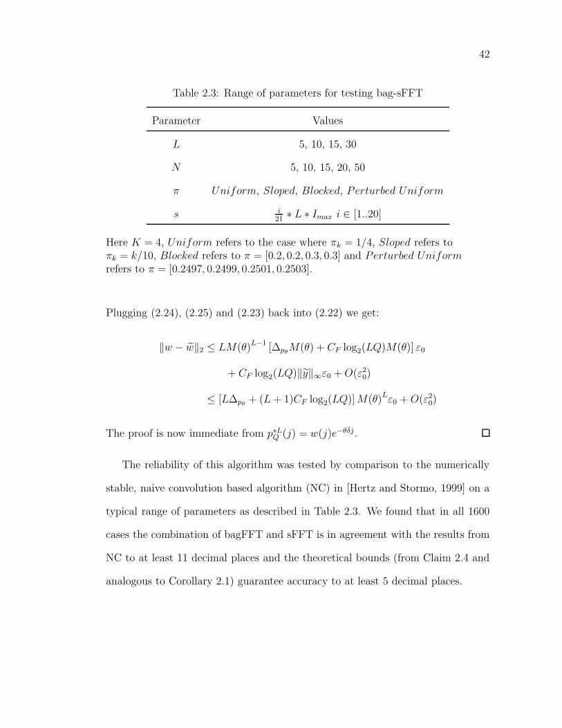
42
Table 2.3: Range of parameters for testing bag-sFFT
Parameter Values
L 5, 10, 15, 30
N 5, 10, 15, 20, 50
π Uniform, Sloped, Blocked, Perturbed Uniform
s i21∗ L ∗ Imax i ∈ [1..20]
Here K = 4, Uniform refers to the case where πk = 1/4, Sloped refers toπk = k/10, Blocked refers to π = [0.2, 0.2, 0.3, 0.3] and Perturbed Uniformrefers to π = [0.2497, 0.2499, 0.2501, 0.2503].
Plugging (2.24), (2.25) and (2.23) back into (2.22) we get:
‖w − w‖2 ≤ LM(θ)L−1 [∆pθM(θ) + CF log2(LQ)M(θ)] ε0
+ CF log2(LQ)‖y‖∞ε0 +O(ε20)
≤ [L∆pθ+ (L+ 1)CF log2(LQ)]M(θ)Lε0 +O(ε2
0)
The proof is now immediate from p∗LQ (j) = w(j)e−θδj .
The reliability of this algorithm was tested by comparison to the numerically
stable, naive convolution based algorithm (NC) in [Hertz and Stormo, 1999] on a
typical range of parameters as described in Table 2.3. We found that in all 1600
cases the combination of bagFFT and sFFT is in agreement with the results from
NC to at least 11 decimal places and the theoretical bounds (from Claim 2.4 and
analogous to Corollary 2.1) guarantee accuracy to at least 5 decimal places.
43
2.8 Conclusion and Future Work
The bagFFT algorithm is asymptotically the fastest algorithm for computing the
exact p-value of the G2 statistic for goodness-of-fit tests. We complement the
algorithm with a rigorous analysis of the accumulation of roundoff errors in it.
Moreover, we show empirically that for a wide range of parameters these error
bounds are useful to guarantee the quality of the computed p-value. We demon-
strate the utility of our approach by combining bagFFT and sFFT to provide a
fast, new algorithm for estimating the significance of sequence motifs. The bagFFT
algorithm is available at http://www.cs.cornell.edu/˜niranjan/.
We are still working on certain algorithmic refinements to bagFFT. In particu-
lar, we wish to optimize bagFFT for computing a single p-value. This is motivated
by Hirji’s algorithm, which as a network algorithm, is optimized for computing
a single p-value based on pruning strategies described in [Hirji, 1997] (another
strategy is described in [Bejerano et al., 2004]). This pruning is one of the main
reasons Hirji’s algorithm is still faster than bagFFT for smaller N . We are cur-
rently working on providing similar runtime gains for bagFFT. Our future goals
include designing a “stitched” algorithm that can choose among a range of existing
algorithms so as to be optimal for any given set of parameter values and a desired
level of accuracy. We would also like to explore the applicability of bagFFT for
Pearson’s X2 and for log-linear models, as well as a generalization to contingency
tables, as is the case for Baglivo et al.’s algorithm [Baglivo et al., 1992].
The bagFFT algorithm serves as another demonstration of the effectiveness of
the shifted-FFT technique [Keich, 2005] to accurately compute vanishingly small
p-values. In recent work, we have studied the applicability of this method to non-
parametric tests such as the Mann-Whitney as well.

44
BIBLIOGRAPHY
[Baglivo et al., 1992] Baglivo,J., Olivier,D. and Pagano,M. (1992) Methods for ex-act goodness-of-fit tests. Journal of the American Statistical Association, 87(418), 464–469.
[Bailey and Elkan, 1994] Bailey,T. and Elkan,C. (1994) Fitting a mixture modelby expectation maximization to discover motifs in biopolymers. In Proceedingsof the Second International Conference on Intelligent Systems for MolecularBiology pp. 28–36 AAAI, Menlo Park, California.
[Bejerano et al., 2004] Bejerano,G., Friedman,N. and Tishby,N. (2004) Efficientexact p-value computation for small sample, sparse and surprising categoricaldata. J. Comput. Biol., 11, 867–886.
[Cressie and Read, 1984] Cressie,N. and Read,T. (1984) Multinomial goodness-of-fit tests. J. R. Statist. Soc. B, 46, 440–464.
[Cressie and Read, 1989] Cressie,N. and Read,T. (1989) Pearson’s χ2 and the log-likelihood ratio statistic g2: a comparative review. International Statistical Re-view, 57 (1), 19–43.
[Dembo and Zeitouni, 1998] Dembo,A. and Zeitouni,O. (1998) Large DeviationTechniques and Applications. Darmstadt, Germany: Springer Verlag.
[Hertz and Stormo, 1999] Hertz,G. and Stormo,G. (1999) Identifying DNA andprotein patterns with statistically significant alignments of multiple sequences.Bioinformatics, 15, 563–577.
[Hirji, 1997] Hirji,K. (1997) A comparison of algorithms for exact goodness-of-fit tests for multinomial data. Communications in Statistics-Simulation andComputations, 26 (3), 1197–1227.
[Hoeffding, 1965] Hoeffding,W. (1965) Asymptotically optimal tests for multino-mial distributions. Annals of Mathematical Statistics, 36, 369–408.
[Keich, 2005] Keich,U. (2005) Efficiently computing the p-value of the entropyscore. Journal of Computational Biology, 12 (4), 416–430.
[Mehta and Patel, 1983] Mehta,C.R. and Patel,N.R. (1983) A network algorithmfor performing fisher’s exact test in r × c contingency tables. Journal of theAmerican Statistical Association, 78 (382), 427–434.

45
[Press et al., 1992] Press,W., Teukolsky,S., Vetterling,W. and Flannery,B. (1992)Numerical recipes in C. The art of scientific computing. Second edition,, Cam-bridge University Press.
[Rahmann, 2003] Rahmann,S. (2003) Dynamic programming algorithms for twostatistical problems in computational biology. In Proceedings of the Third In-ternational Workshop on Algorithms in Bioinformatics (WABI-03), (Benson,G.and Page,R.D.M., eds), vol. 2812, of Lecture Notes in Computer Science pp.151–164 Springer, Budapest, Hungary.
[Sadreyev and Grishin, 2004] Sadreyev,R.I. and Grishin,N.V. (2004) Estimates ofstatistical significance for comparison of individual positions in multiple sequencealignments. BMC Bioinformatics, 5 (106).
[Siotani and Fujikoshi, 1984] Siotani,M. and Fujikoshi,Y. (1984) Asymptotic ap-proximations for the distributions of multinomial goodness-of-fit statistics. Hi-roshima Math. J., 14, 115–124.
[Stormo, 2000] Stormo,G. (2000) DNA binding sites: representation and discovery.Bioinformatics, 16 (1), 16–23.
[Tasche and Zeuner, 2001] Tasche,M. and Zeuner,H. (2001) Worst and averagecase roundoff error analysis for fft. BIT, 41 (3), 563–581.

CHAPTER 3
COMPUTING THE SIGNIFICANCE OF AN UNGAPPED LOCAL
ALIGNMENT
3.1 Introduction
Finding local similarities among a set of sequences is a common task in compu-
tational biology. For example, by finding similarities within a set of promoters
from coregulated genes, one hopes to recover transcription factor binding sites
that guide the genes’ expression patterns in vivo. Given a set of sequences,
motif finding algorithms such as MEME [Bailey and Elkan, 1994] and CONSEN-
SUS [Hertz and Stormo, 1999] return a number of possible alignments in some
order of potential biological relevance. A critical part of any such study is for a
researcher to discriminate between local alignments that are simply random arti-
facts of the sample, and local alignments that are so improbable by chance that
they are likely to be biologically relevant.
An ungapped local alignment of length L of sequences from an alphabet with A
letters is typically summarized by its information content, or entropy [Stormo, 2000]
as follows. Let nij denote the number of occurrences of the jth letter in the ith
column of the alignment, and let n be the number of sequences in the alignment.
The entropy score, or information content, of the alignment is defined as
I :=L∑
i=1
A∑
j=1
nij lognij/n
bj,
where bj is the background frequency of the jth letter (typically, bj is the frequency
of the jth letter in the entire sample).1 The entropy score for a given column i of
1Strictly speaking, relative entropy is defined as I/n.
46

47
the alignment is defined, similarly, as:
I(i) :=
A∑
j=1
nij lognij/n
bj.
While this score can be used to rank more than one alignment in a given sample,
it cannot provide any direct information about an alignment’s significance, and in
particular cannot be used to compare two alignments of varying L and n. To assess
the significance of an alignment with entropy score s0, we rely on the alignment’s
p-value, which is the probability of seeing an entropy score of s0 or better under
the assumption that each of the L columns has n letters independently sampled
according to the background distribution {b1, . . . , bA}. If the p-value is near 1 then
the columns in the alignment are too similar to the background for the pattern to
be interesting, but if the p-value is near 0 then the alignment suggests a functional
site.
Let p denote the probability mass function (pmf) of the column score I(i) under
the hypothesis that the column is noise—in the sense that it was sampled from the
multinomial distribution described by the background probabilities {b1, . . . , bA}.
Assuming that the entropy score for each of the L columns in the alignment is an
independent random variable, the pmf of the alignment’s total entropy score I is
given by the L-fold convolution of p:
p∗L(s) := p ∗ · · · ∗ p︸ ︷︷ ︸L
:=∑
(s1,...,sL):s1+···+sL=s
p(s1) . . . p(sL). (3.1)
The p-value of an alignment with score s0 is therefore F ∗L(s0) :=∑
s≥s0 p∗L(s).
Unfortunately, to naively compute this requires traversing all s ≥ s0, which is
prohibitively expensive in practice because of the large number of possible values
of s. As a result, multiple alignment programs rely on approximations to compute

48
the p-value, striving for a balance between the time spent computing and the
accuracy of the result.
To determine if approximating the p-value computation introduces errors in
practice, Jones and Keich [Jones and Keich, 2005] modified the source code of
MEME (version 3.0.3) and CONSENSUS (version 6c, April 2001) to score arbitrary
alignments, bypassing each algorithm’s motif finding step. In this way they were
able to compare p-value estimates from different algorithms on a variety of different
alignments. Figure 3.1 shows the results from their experiments where a point at
(x, y) is plotted for an alignment with CONSENSUS E-value of x and a MEME
E-value of y. The E-value of an alignment with score s0 is the expected number
of alignments in the sample with the same n and L and with entropy score greater
than or equal to s0. It can be obtained from the p-value by multiplying by the
number of possible alignments in the sample. As can be seen in the figure, the
MEME E-value is consistently larger than the CONSENSUS E-value (which is
reliable in this region) by roughly two orders of magnitude. Jones and Keich
found that in at least one case, the true E-value indicates an expectation of 10
alignments with comparable score existing in the sample, while MEME reports an
expectation of 5000 alignments; it is conceivable that a researcher would arrive at
two different conclusions about the significance of the same alignment by relying
on the two estimates. Furthermore, they found at least two alignments of the
same size that had inconsistent E-values according to MEME: one alignment had
a lower entropy and also a lower E-value than the other (entropy of 13.583, E-
value of 1.725× 10⁷ compared to entropy of 13.617, E-value 4.1716× 10⁷) which
is clearly a contradiction. Neither the approximation methods discussed in this
chapter, nor the methods proposed in [Hertz and Stormo, 1999] demonstrate this

49
-4
-2
0
2
4
6
8
10
12
-4 -2 0 2 4 6 8 10 12
log 10
(MEM
E E-
valu
e)
log10(Consensus E-value)
y=x
Figure 3.1: A comparison of MEME E-values to CONSENSUS E-values
The comparison was done for L = 15 and n = 20 where the sequences are oflength 1000 each. Since the CONSENSUS E-values are accurate over the rangeof scores considered here, MEME clearly overestimates the E-value in nearlyevery case; for alignments with E-values smaller than or equal to 1 according toCONSENSUS, MEME may report an E-value as large as 100.
instability.
It is important to note that the E-values from CONSENSUS were calculated
using an algorithm (LD; see below) that is fast but at times inaccurate. An example
of the ratio of CONSENSUS p-values to the true p-values (as calculated by the
slower but accurate NC algorithm; see below) is shown in Figure 3.2. Since the
CONSENSUS-reported estimates can be up to two orders of magnitude off, this
chapter introduces a compromise that achieves nearly the accuracy of NC, but at
speeds comparable to LD.
[Hertz and Stormo, 1999] suggest two possible approximation techniques for

50
398 400 402 404 406 408 410 412 414 416 418−1
−0.5
0
0.5
1
1.5
2
Score (s)
10lo
g (
LD(s
)/NC(
s))
Figure 3.2: Graph of log10(LD(s)/NC(s))
This graph demonstrates how far off the CONSENSUS-reported p-value may befrom the value it estimates. The parameters for this graph are n = 20, A = 4,L = 10 and b = [0.2497, 0.2499, 0.2501, 0.2503]. The gaps in the graph indicateareas of unattainable entropy values.

51
calculating the p-value. The first, NC, replaces I(i) with its latticed cousin Iδ(i) :=
bI(i)/δc. In this case, the L-fold convolution of pδ (the pmf of Iδ(i)) can be
done more efficiently than the L-fold convolution of p and is used to approximate
it. A naive algorithm for computing the L-fold convolution on a lattice requires
O(L2M2) time, where M is the size of the lattice. Hertz and Stormo note that using
the Fast Fourier Transform (FFT) to perform the convolution would decrease the
running time to O(LM log(LM)); however, the numerical instability of the FFT
algorithm tends to wreak havoc on the computation’s accuracy for small values,
which is exactly the region we are most interested in when searching for motifs. The
second method they suggest, LD, uses large deviation theory to estimate the tail
of an exponentially shifted probability distribution. In practice this approximation
scheme works quite well except for a range of values near the maximal (or minimal)
score where it may be off by an order of magnitude or more. Nevertheless, LD
is nearly 200 times faster to compute than NC for L = 10, A = 4, n = 100 and
M = 16384 and is therefore the method used in the popular CONSENSUS tool.
As an alternative to NC, [Keich, 2005] proposes the sFFT algorithm to over-
come the numerical instability of the FFT for the L-fold convolution step and also
delineates explicit bounds on the accuracy of the result. Though this method has
lower complexity than NC, it is still somewhat time consuming on large sample
sizes. In Section 3.2, we present improvements to sFFT that give rise to the fastest
known algorithm that has accuracy comparable to NC. We then describe an opti-
mization, the cyclic-shifted-FFT technique, to produce the csFFT algorithm which
is more efficient for the computation of a single p-value, with speed comparable to
LD.

52
3.2 Methods
Following the treatment in [Keich, 2005], we introduce the shifted-FFT (sFFT)
algorithm. The primary bottleneck of the algorithm presented in that paper is the
computation of the probability mass function of one column’s entropy score, which
we show here can be done much more efficiently.
3.2.1 The Shifted-FFT (sFFT) algorithm
The L-fold convolution of an arbitrary vector v ∈ CM , written v∗L, can be com-
puted as follows. Let N = ML and extend v to N dimensions by padding it with
zeros. Define w ∈ CN as w(k) = [(Dv)(k)]L (where D and D−1 are the DFT
operator and its inverse respectively as defined in Section 2.3). Then v∗L is given
by v∗L(l) := (D−1w)(l).
The straightforward implementations of D and D−1 require O(N 2) time, but
using a recursive divide-and-conquer strategy results in the Fast Fourier Transform
(FFT) which takes O(N logN) time. If D and D−1 are the respective implemen-
tations of D and D−1, then as shown in Section 2.4, due to numerical errors D
and D−1 are not exactly the linear and mutually inverse operators that D and
D−1 are. Correspondingly, this naive FFT based computation cannot recover v∗L
accurately.
To avoid the problem of roundoff errors in computing the L-fold convolution of
pδ, we can emphasize the values of pδ in the region surrounding s0 by applying an
appropriate exponential shift prior to performing the L-fold convolution. Let
pθ,δ(s) := pδ(s)eθs/Mδ(θ), (3.2)
where Mδ(θ) = E[eθIδ(i)
]is the moment generating function of the lattice score

53
for one column. This particular form of shifting commutes with the convolution
operator which makes it easy to convert between p∗Lθ,δ and p∗Lδ . Note that, as s is
latticed, pθ,δ is an M -dimensional vector. We will use the notation pθ,δ(j) to refer
to the jth entry in that vector, and pθ,δ(s) to refer to the value of pθ,δ for entropy
score s.
Since θ is a parameter, we can choose it in such a way that for a given alignment
score s0 we get the maximal ”resolving power” relative to noise due to numerical er-
ror in the DFT. Intuitively, the most significant contributions to the p-value should
come from values of p∗Lδ close to s0, so we choose to center the mean of the shifted
pmf for one column at s0/L so that p∗Lθ,δ is centered about s0. This can be satis-
fied, based on a standard large deviation procedure [Dembo and Zeitouni, 1998],
by setting
θ0 = argminθ [logMδ(θ)− θs0/L] . (3.3)
Of course, in order to proceed with the convolution, we need an estimate for
the pmf of a single column. This could be performed by naively enumerating
all possible empirical distributions for a column. While this approach has the
advantage of being the most accurate, it requires O(nA−1) time. For small values
of A (as is the case for nucleotide sequences) this algorithm is still computationally
tractable. However, in our experiments we found that even for small values of n,
with A = 4, this stage tends to dominate the runtime of the algorithm.
An algorithm with runtime O(AMn2) to calculate the pmf on a lattice was
proposed by Hirji [Hirji, 1997]2. This particular algorithm produces the pmf over
the entire range of possible values in one execution by using dynamic programming.
An improvement to the runtime of the algorithm can be obtained by noting that for
2It was later rediscovered by Hertz and Stormo [Hertz and Stormo, 1999].

54
small values of n, the number of non-zero lattice points in the intermediate stages
of the calculation is small, which allows one to employ a list-based data structure
to reduce the runtime to O(AM ′n log(n)) where M ′ is significantly smaller than
M in practice (< 10 for the parameters in Table 3.1). The resulting algorithm is
more efficient than the original but it still suffers from the overhead of computing
with log-values 3 in order to avoid underflows.
The underflow conditions in Hirji’s algorithm arise because it multiplies and
adds terms of the form ra(n′) = ba
n′
/n′! (where ba is the background distribution
for a ∈ [1..A] and n′ ∈ [0..n]) that are exponentially small in n′. These terms are
used to recursively compute the vector pδ,a,n′, where
pδ,a,n′(j) =n′∑
n′′=0
ra(n′′) · pδ,a−1,n′−n′′(j − ja(n′′)) (3.4)
pδ,1,n′(j) =
n! · r1(n′) if j = ja(n′) and n′ ∈ [0..n]
0 otherwise
and ja(n′) = round(δ−1n′ log(n
′/nba
)). As is shown in [Hertz and Stormo, 1999],
pδ(j) = pδ,A,n(j) and so this procedure recovers the pmf pδ.
In order to avoid the use of logarithms in these computations we design the
following procedure: instead of computing with the ra’s we shift them to get
r′a(n′) = ra(n
′)eδja(n′)+n′(log(n)−1)
and perform the recursion in (3.4) using r′a’s. Let the corresponding result be p′δ.
We can then recover pδ based on the following claim:
Claim 3.1. pδ(j) = p′δ(j)e−δj−n(log(n)−1)
3Addition of log-values in a C program, for example, was found to be more than10 times slower than regular addition.

55
0
0.5
1
1.5
2
2.5
3
0 50 100 150 200 250 300 350 400
Runt
ime
(in se
cs)
Number of sequences (n)
Runtime comparison of shifted-Hirji with log-Hirji and bagFFT
shifted-Hirjilog-HirjibagFFT
Figure 3.3: Runtime comparison for versions of Hirji’s algorithm and bagFFT
The paramters for this comparison are A = 4, M = 1024 and the uniformbackground distribution.
The proof of this claim is based on simple induction using (3.4) and is therefore
omitted.
The shifted computation described above (shifted-Hirji) avoids the underflow
conditions of Hirji’s original algorithm. This is because, even though ra(n′) de-
creases exponentially with respect to n′, r′a(n′) remains approximately 1√
2πn′. For
practical values of n this improvement to Hirji’s algorithm does not introduce any
numerical errors into the result, and in some cases it may be more accurate than
relying on logarithms (we refer to this version as log-Hirji). As can be seen from
Figure 3.3, it also substantially improves the runtime (by more than a factor of 10,
on average). Note that, as shown in Chapter 2, bagFFT is asymptotically more

56
0
1
2
3
4
5
6
7
8
9
20 40 60 80 100 120 140 160
Runt
ime
(in se
cs)
Number of sequences (n)
Runtime comparison of shifted-Hirji with bagFFT for A=20
shifted-HirjibagFFT
Figure 3.4: Runtime comparison of shifted-Hirji and bagFFT for A = 20
The paramters for this comparison are M = 16384 and the uniform backgrounddistribution.
efficient than Hirji’s algorithm and can be combined with sFFT to compute the
significance of motif scores. However, as illustrated by Figure 3.3, shifted-Hirji
can be more efficient than bagFFT for A = 4 and the values of n that we are
typically interested in for finding transcription factor binding sites. The practical
advantages of bagFFT over shifted-Hirji are more evident for larger A (as in the
case of protein alignments) and n as is suggested by Figure 3.4.
The modified sFFT algorithm is shown in Figure 3.5. It is important to note
that the proof of correctness for the original sFFT algorithm [Keich, 2005] is triv-
ially extended to this case where the complete enumeration of the pmf is replaced
with the shifted-Hirji algorithm4. Thus, this version of the sFFT algorithm is
4The original bounds on the p-value are now replaced with looser bounds

57
The input to sFFT is:
• n, the number of sequences
• L, the number of columns in the alignment
• b1, . . . , bA, the background frequencies of the A letters
• M , the size of the lattice
• s0, the observed score
Given the input, sFFT:
1. Computes pδ, an estimate of pδ by using the shifted-Hirji algorithm.
2. Finds θ0 by numerically solving (3.3).
3. Computes pθ0,δ(s) according to (3.2).
4. Computes p∗Lθ0,δ by applying the FFT-based convolution to pθ0,δ(s).
5. Computes p∗Lδ (j) = p∗Lθ0,δ(j)e−θ0jδ+L log fMδ(θ0) for j0 ≤ j ≤ jmax,
where j0 and jmax are the lattice indices corresponding to s0 and
the maximum score smax.
6. Returns sFFT(s0) :=∑jmax
j=j0p∗Lδ (j).
Figure 3.5: The sFFT algorithm
faster than the original, yet just as reliable.
3.2.2 The Cyclic Shifted-FFT (csFFT) algorithm
The sFFT algorithm above can compute p-values for a range of possible alignment
scores, which is wasteful when all we need is a single p-value. Fortunately, most
of the mass of the shifted probability mass function p∗Lθ,δ arises from a restricted
range of possible s-values as Figure 3.6(a) suggests.

58
0 5 10 15x 104
0
1
2
3
4
5
6x 10⁻³
j
p θ,δ
∗ L (j)
pθ,δ∗ L
(L−1)M
(a) An example where p∗Lθ,δ has its es-
sential support in a narrow interval
defined by [(L−1)M,LM ]; s0 = 405.
0 5 10 15x 104
0
1
2
3
4
5
6x 10⁻⁵
j
p θ,δ
∗ L (j)
pθ,δ∗ L
(L−4)M
(b) Here, p∗Lθ,δ has its essential sup-
port in an interval larger than M ,
defined by [(L−4)M,LM ]; s0 = 350.
0 5 10 15x 104
0
0.5
1
1.5
2
2.5
3
3.5
4
4.5x 10⁻⁵
j
p θ,δ
∗ L (j)
pθ,δ∗ L
(L−7)M(L−2)M
L’M
(c) The support for p∗Lθ,δ is mainly in
an L′M interval for L′ = 5, but not of
the form [(L−L′)M,LM ]; s0 = 300.
Figure 3.6: The shifted pmf is 0 for much of the valid values of s
Here, M = 10000, n = 20, L = 15, b = [0.2499, 0.2501, 0.2497, 0.2503]. The“essential support” intervals here are described by indices for the latticed pmf.
59
We would like to avoid computing p∗Lθ,δ on those large intervals where it is practically
zero. To that end, consider the following cyclic sum of p∗Lθ,δ :
q(i) =∑
{j:j mod M=i}p∗Lθ,δ(j). (3.5)
In the example described in Figure 3.6(a), p∗Lθ,δ ≈ 0 for j /∈ [(L− 1)M,LM ]; there-
fore, it follows that q(i) (where i = j mod M) approximates p∗Lθ,δ(j) on the interval
j ∈ [(L − 1)M,LM ]. Since q is defined on a lattice of size M rather than on a
lattice of size LM , we can immediately save a factor of L, provided q is efficiently
computable. Since q is the cyclic convolution of pθ,δ it can be efficiently computed
by:
Claim 3.2. q = D−1M w, where w(k) =
[(DM pθ,δ
)(k)
]L.
The proof of this claim can be found in [Press et al., 1992]. The difference
between the formula above and its non-cyclic analog is the dimensionality of the
DFT operator: here it is M while the DFT operator previously had dimensionality
LM with pθ,δ appropriately padded with (L− 1)M zeros.
More generally, the essential support interval of p∗Lθ,δ may be of size L′M (for
example, see Figure 3.6(b)). Such an interval may also not be strictly of the form
[(L−L′)M,LM ]; instead being centered about s0 (for example, see Figure 3.6(c)).
In this case, rather than directly calculating
F ∗Lδ (j0) :=
∑
j≥j0p∗Lδ (j)
we approximate it with
F ∗Lθ (j0) :=
∑
j0≤j≤Jq(j)e−θ0jδ+L logM(θ0)

60
where J = min(j0 + L′M/2, jmax). This is justified by
∑
j0≤j≤Jq(j)e−θ0jδ+L logM(θ0)
≈∑
j0≤j≤Jp∗Lθ,δ(j)e
−θ0jδ+L logM(θ0)
≈∑
j≥j0
p∗Lθ,δ(j)e−θ0jδ+L logM(θ0)
An appropriate choice of L′ would ensure that, say, 95% of the mass of p∗Lθ,δ
lies in the interval of size L′M centered about j0. This would be relatively easy
if we had an explicit function for p∗Lθ,δ, but this is exactly the function we are
trying to estimate. Instead, we rely on the following formula for L′, under the
assumption that p∗Lθ,δ is roughly normally distributed (an assumption made by the
LD algorithm):
L′ :=
⌈kσ√LσθM
⌉. (3.6)
Here, σ2θ := Var pθ,δ, where pθ,δ is the integer lattice version of (3.2) and the
variance is computed on the lattice indices. Note that kσ√Lσθ = kσ
√Var(p∗Lθ,δ) so
an interval of size L′M centered about j0 extends roughly kσ/2 standard deviations
on each side. Thus, if we arbitrarily set kσ := 4, then (3.6) roughly ensures the
desired 95% condition under the assumption of normality.
3.2.3 Boosting θ
As observed in [Hertz and Stormo, 1999], when s approaches smax, θ increases
while σθ decreases. Thus, for s0 close to smax, if we increase or boost θ beyond
the computed θ0 = θ(s0) from (3.3), we reduce σθ. Since L′ depends linearly on
σθ (from (3.6)), such boosting can effectively decrease the runtime by reducing L′.
Another reason to boost θ for s near smax is that it reduces the error introduced
by approximating sFFT with the cyclic sum in csFFT, as shown next.

61
Claim 3.3. Let d = L′M , J ′ = min (j0 + d− 1, jmax) and j ′ ≡ j mod d. Then
F ∗Lθ (j0)− F ∗L
δ (j0) ≤∑
j0≤j≤J
∑
j′<j
p∗Lδ (j ′)e−θ0(j−j′)δ (3.7)
+∑
j0≤j≤J
∑
j′>j
p∗Lδ (j ′)(e−θ0(j−j′)δ − 1) (3.8)
F ∗Lδ (j0)− F ∗L
θ (j0) ≤∑
j0+d/2<j≤J ′
∑
j′>j
p∗Lδ (j ′) (3.9)
The proof of the claim is straightforward from the definitions and is therefore
omitted.
Suppose s is sufficiently close to smax so that j0 + d/2 > jmax. In that case the
right hand side of (3.9) vanishes leaving F ∗Lθ (j0) as an upper bound of the p-value,
F ∗Lδ (j0). Moreover, the term (3.8) vanishes as well and we are left with:
0 ≤ F ∗Lθ (j0)− F ∗L
δ (j0) (3.10)
≤∑
j0≤j≤jmax
∑
j′<j
p∗Lδ (j ′)e−θ0(j−j′)δ. (3.11)
This upper bound on the error decreases as θ0 increases, which supports our as-
sertion that boosting θ is beneficial for s close to smax.
One might be tempted to boost θ by a large amount, but while this would indeed
reduce the error in (3.11) it would have the unfortunate side effect of increasing
the numerical errors in the FFT (discussed at length in [Keich, 2005]).
An intermediate solution is to boost θ by adding
θboost = log(109)/((jmax − j0)δ). (3.12)
This solution can boost θ significantly and bring corresponding savings in runtime,
as well as reduce the error in (3.11). It is also designed (based on some assumptions
about p∗Lθ,δ) to still preserve the important entries of p∗Lθ,δ (for computing the p-value)
during the FFT. Finally, while this solution is heuristic, it works well in practice,
as is shown in Sections 3.3.1 and 3.3.2.

62
The input to csFFT is:
• n, the number of sequences
• L, the number of columns in the alignment
• b1, . . . , bA, the background frequencies of the A letters
• M , the size of the lattice
• s0, the observed score
Given the input, csFFT:
1. Computes pδ, an estimate of pδ by using the shifted-Hirji algorithm.
2. Finds θ0 by numerically solving (3.3).
3. Computes L′ according to (3.6) and using the default kσ = 4.
4. Boosts θ0 by (3.12) if j0 + L′M/2 > jmax.
5. Computes pθ0,δ(s) according to (3.2).
6. Computes p∗Lθ0,δ by applying the FFT-based cyclic-convolution to pθ0,δ(s)
with period L′M .
7. Computes p∗Lδ (j) = p∗Lθ0,δ(j)e−θ0jδ+L log fMδ(θ0) for j0 ≤ j ≤ J .
8. Returns csFFT(s0) :=∑J
j=j0p∗Lδ (j).
Figure 3.7: The csFFT algorithm

63
The cyclic shifted FFT algorithm (csFFT) with boosting is shown in Figure 3.7.
For typical values of L, the csFFT algorithm is simultaneously more accurate than
and comparable in speed to LD.
3.3 Results
3.3.1 Runtime characterization
Assuming that the time-limiting step of sFFT is the calculation of the FFT itself,
csFFT is roughly L/L′ times faster than the sFFT algorithm described in the
previous section. Interestingly, the savings of L/L′ varies with s0: the speedup for
values of s0 near the center of the distribution is modest, while the best gains occur
near the ends of the range of possible s-values. This follows from the fact that as
s0 approaches smax (or smin), the corresponding σθ goes to 0 yielding a smaller L′
in (3.6). In any case, the complexity of csFFT is lower than that of sFFT: by (3.6)
the complexity of the FFT step is now O(√LM log(
√LM)).
We conducted tests to verify that csFFT is indeed more efficient than sFFT.
Since sFFT and csFFT differ mainly in the convolution step of the algorithm
where the running times are roughly linear in L and L′ respectively, we focus on
the growth of L′ in terms of L. Figure 3.8(a) demonstrates that if we take the
average value of L′ over the range of s values, it grows roughly as√L when all
other parameters are fixed. In addition, the average value of L′ is roughly constant
for different ba’s from Table 3.1 (based on a test with L = 10 and n = 10) and
decreases as n increases5 (see Figure 3.8(b)). Furthermore, we found that boosting,
when it is applicable, gives substantial runtime gains; halving the runtime in many
5In practice the runtime increases with n as we have to increase M proportion-ally to maintain the granularity of the lattice.

64
1.5
2
2.5
3
3.5
4
4.5
5
5.5
6
0 5 10 15 20 25 30 35 40 45 50
Ave
rage
L’
Length of alignment (L)
Average L’ as a function of L
Avg L’
(a) n = 10 and M = 16384.
2.4
2.45
2.5
2.55
2.6
2.65
2.7
2.75
2.8
2.85
2.9
5 10 15 20 25 30 35 40 45 50
Ave
rage
L’
Number of sequences (n)
Average L’ as a function of n
Avg L’
(b) L = 10 and M = 16384.
Figure 3.8: Average values of L′ versus L and N
The results were obtained using the perturbed Uniform ba and the averages aretaken over 100 evenly spaced values of s.
cases. Finally, since csFFT relies on a substantially faster convolution than sFFT,
we found that for tests with large n, small L and s close to smax the runtime of the
algorithm is no longer dominated by the time for the convolution. For example, in
a test case with n = 20, L = 15, ba = Uniform, M = 16384 and s = 380, csFFT
takes 0.09s to compute the answer, of which 0.01s is spent in the shifted-Hirji
step, 0.07s is spent computing the shift, and 0.01s is required for the cyclic-FFT
(L′ = 2). New techniques to reduce the time spent in computing the shift could
be a useful addition to the algorithm.
3.3.2 Error analysis
For each combination of parameter values in Table 3.1 we tested 20 roughly evenly
spaced values for s and separately another set of 100 points lying in the tail of the
pmf. Because we have latticed s, the p-value of s has an inherent lattice error, as

65
Table 3.1: Range of test parameters
Parameter Values
L 5, 10, 15, 30
n 2, 5, 10, 15, 20, 50
ba Uniform, Sloped, Blocked,
Perturbed Uniform
Uniform refers to the case where b = [0.25, 0.25, 0.25, 0.25], Sloped refers tob = [0.1, 0.2, 0.3, 0.4], Blocked refers to b = [0.2, 0.2, 0.3, 0.3] and PerturbedUniform refers to b = [0.2497, 0.2499, 0.2501, 0.2503].
discussed in [Keich, 2005]. For any given value of s, sFFT(s) and csFFT(s) fall
within a small range; the true value falls somewhere in between the minimum and
maximum values in that range. The bounds for the p-values computed by csFFT
was then compared to the provably reliable bounds from sFFT. In all cases that
we tested, we found that the bounds agreed to more than 1 decimal place. The
cases with the worst disagreement were usually found to be for values of s close to
the average of the pmf where the p-values are large and therefore not very relevant
in most applications.
3.3.3 Stitching LD and csFFT
The csFFT algorithm is simultaneously more accurate than and comparable in
speed to LD. For example, for L = 10, n = 100, ba = Uniform, M = 16384 and
s = 380, CONSENSUS’s p-value computation required 0.32s, while csFFT required
0.20s with L′ = 3. Admittedly, this is a somewhat biased example as n = 100 is
likely larger than typical problems. For the example in the previous section, on the

66
Table 3.2: Runtime comparison between csFFT and LD
n L s Runtime for csFFT Runtime for LD
(in seconds) (in seconds)
40 5 200 0.04 0.06
15 5 100 0.01 0.01
15 30 600 0.05 0.01
40 30 600 0.12 0.06
40 5 260 0.02 0.06
The comparisons were made using the Uniform ba (see Table 3.1) and with Q setto 16384.
other hand, LD is faster by a factor of 4. We present a few more examples in Table
3.2. In general, LD is faster than csFFT for small n and large L and also for values
of s that are away from the tail with larger L′. We can exploit this by designing a
heuristic rule that switches to LD for appropriate values of n and L. In designing
a switching criterion we also need to consider the approximation errors inherent
to LD; an example is given in the introduction in which LD gives a very poor
approximation. [Hertz and Stormo, 1999] present an empirical test that can be
used to gauge the reliability of the LD-based normal approximation. Essentially, if
s is less than 3 standard deviations (of the shifted pmf) from smax then the normal
approximation is no longer reliable. We calculated the observed error of the LD
method in the range defined by this test for the set of parameters in Table 3.1 and
found that in all cases the error ratio was less than 1.24, corresponding to less than
24% error. We can therefore use this test in conjunction with csFFT to yield an
algorithm that is efficient and accurate over a larger range of n and L values.

67
3.4 Conclusion
Accurate methods for estimating the p-value of an alignment score are critical
in aiding the discovery of biologically meaningful signals from sets of related se-
quences. While existing tools provide estimates, it is clear that some estimates are
better than others. The method employed by MEME is overly pessimistic about an
alignment, which could conceivably lead to missed signals. While the method used
by CONSENSUS is more accurate, it can still improperly estimate the p-value.
Two methods were presented in this chapter that work well in practice for DNA
motifs. While the first (sFFT) is not quite as fast as LD, it is significantly faster
than NC, has bounded error estimates, and returns p-values for a range of entropy
scores. The second, csFFT, is comparable in speed to LD and is empirically more
accurate, but like LD returns a p-value only for a single entropy score.
The algorithms described in this chapter provide a general method for the
computation of p-values for ungapped alignments. Extending these methods to
account for gapped alignments is, however, an important and interesting topic
for future research. The methods described in this chapter can also be used for
applications other than motif finding. These tools may be helpful wherever a sta-
tistical significance of a multiple alignment is desired; for example, in the problem
of profile-profile alignment or in the analysis of protein families.

68
BIBLIOGRAPHY
[Baglivo et al., 1992] Baglivo,J., Olivier,D. and Pagano,M. (1992) Methods for ex-act goodness-of-fit tests. Journal of the American Statistical Association, 87(418), 464–469.
[Bailey and Elkan, 1994] Bailey,T. and Elkan,C. (1994) Fitting a mixture modelby expectation maximization to discover motifs in biopolymers. In Proceedingsof the Second International Conference on Intelligent Systems for MolecularBiology pp. 28–36 AAAI, Menlo Park, California.
[Dembo and Zeitouni, 1998] Dembo,A. and Zeitouni,O. (1998) Large DeviationTechniques and Applications Second edition,, Springer-Verlag, NY, USA.
[Jones and Keich, 2005] Jones, N.C., and Keich, U. (2005) Personal Communica-tion.
[Hertz and Stormo, 1999] Hertz,G. and Stormo,G. (1999) Identifying DNA andprotein patterns with statistically significant alignments of multiple sequences.Bioinformatics, 15, 563–577.
[Hirji, 1997] Hirji,K. (1997) A comparison of algorithms for exact goodness-of-fit tests for multinomial data. Communications in Statistics-Simulation andComputations, 26 (3), 1197–1227.
[Keich, 2005] Keich,U. (2005) Efficiently computing the p-value of the entropyscore. Journal of Computational Biology, 12 (4), 416–430.
[Keich and Nagarajan, 2004] Keich,U. and Nagarajan,N. (2004) A faster reliablealgorithm to estimate the p-value of the multinomial llr statistic. In Proceedingsof the fourth Workshop on Algorithms in Bioinformatics (WABI-04).
[Press et al., 1992] Press,W., Teukolsky,S., Vetterling,W. and Flannery,B. (1992)Numerical recipes in C. The art of scientific computing. Second edition,, Cam-bridge University Press.
[Stormo, 2000] Stormo,G. (2000) DNA binding sites: representation and discovery.Bioinformatics, 16 (1), 16–23.

CHAPTER 4
REFINING MOTIF FINDERS WITH E-VALUE CALCULATIONS
4.1 Introduction
The problem of motif finding can be summarized as scanning a given set of se-
quences for short, well-conserved ungapped alignments. Most of the interest in this
problem comes from its application to identification of transcription factor binding
sites, and of cis-regulatory elements in general. These in turn are important to
the fundamental problem of understanding the regulation of gene expression. This
motivated the design of several popular motif finding tools that search for short
sequence motifs given only an input set of sequences (see [Tompa et al., 2005] for
a recent comparative review).
Most existing motif finders can be divided into two classes depending on whether
they model a motif with a consensus sequence or with a position weight matrix
(PWM or profile). Commonly used motif finders that fall in this latter category
include MEME [Bailey and Elkan, 1994], CONSENSUS [Hertz and Stormo, 1999]
and the various approaches to Gibbs sampling (for example [Lawrence et al., 1993,
Neuwald et al., 1995, Hughes et al., 2000]). This chapter concentrates on improv-
ing this popular class of finders.
Profile-based motif finding algorithms typically try to optimize the entropy
score, or information content of the reported alignment (as defined in Chapter
3). In order to assign statistical significance to the reported motifs as well as to
be able to compare alignments of different widths and depths Hertz and Stormo
introduced the notion of a motif E-value. Introduced originally in this context as
the “expected frequency” [Hertz and Stormo, 1999], the E-value is the expected
69

70
number of random alignments of the same dimension that would exhibit an entropy
score that is at least as high as the score of the given alignment. When the E-value
is high, one can have little confidence in the motif prediction, and conversely when
the E-value is low, one can have more confidence in the prediction. It is computed
by multiplying the number of possible alignments by the p-value of the alignment
(which is the subject of Chapter 3). The latter is defined as the probability that
a single given random alignment would have an entropy score ≥ the observed
alignment score.
While the E-value is the chosen figure-of-merit for evaluating motifs in popular
motif finders such as MEME and CONSENSUS it is not directly optimized for.
For example, in MEME E-values are only computed after the EM-algorithm com-
pletes its optimization and are only used for significance evaluation and possibly
for comparing motifs of different widths. Similarly, when CONSENSUS looks to
extend a sub-alignment (matrix) in its greedy search strategy, it chooses the one
that optimizes the entropy rather than the E-value1. One of the main reasons for
this separation between optimization and significance analysis is that E-values are
significantly more expensive to compute than entropy scores. Even the relatively
fast (and potentially inaccurate as shown in Chapter 3) large-deviation method
that CONSENSUS employs for computing the E-value can tax an optimization
procedure at an unacceptable level.
The discussion above raises two questions:
• Cost aside, can a more direct optimization of the E-value improve our results?
• Can we compute the E-values efficiently so that they can be optimized for?
1These two approaches would generally differ if the lengths of the sequences arenot identical.

71
This chapter lays out arguments advocating a positive answer for both questions.
We begin by describing a new technique, memo-sFFT (based on the techniques
in Chapter 3), that allows us to accurately and efficiently compute multiple E-
values. We then present the Conspv program that uses the memo-sFFT system
to implement a CONSENSUS style motif finder that directly optimizes E-values.
The Conspv program generalizes readily to the problem of finding motifs of un-
known widths and is functionally equivalent to a combination of CONSENSUS
and WCONSENSUS [Hertz and Stormo, 1999]. We show based on experiments
on synthetic data that Conspv can significantly improve over WCONSENSUS
for finding motifs of unknown widths. As further evidence to the advantage of
a more direct optimization of the E-values, we describe the Gibbspv algorithm
[Ng and Keich, 2006]. This new variant of the Gibbs-sampling algorithm is es-
pecially effective when searching for motifs of unknown width by incorporating
memo-sFFT to efficiently consider E-values in its optimization procedure. In our
experiments on synthetic datasets, Gibbspv clearly outperforms other motif finders
for finding motifs of unknown width.
It should be noted that GLAM [Frith et al., 2004] is conceptually quite similar
to Gibbspv as both rely on a Gibbs sampling procedure to optimize an overall mea-
surement of statistical significance. However GLAM uses a different significance
analysis and as we show below in our tests it is less successful than both Conspv
and Gibbspv.
4.2 Efficiently computing E-values
In a typical application of CONSENSUS in the experiments described in Section 4.6
about 108 alignments are compared. CONSENSUS compares them using entropy

72
scores that can be computed in O(wn + wA) time from scratch, where w is the
width of the motif, n is the number of sequences and A is the alphabet size (in this
chapter a DNA alphabet of 4 letters). Note that the typical case in CONSENSUS
is actually when the score is updated while extending a sub-alignment and this
takes O(w) time. In comparison, computing E-values reliably can be many orders
of magnitude more expensive if done naively. An efficient algorithm for reliably
computing a single p-value (a crucial time-limiting step for computing E-values,
see [Hertz and Stormo, 1999]) can typically take ≈ 0.01s for the test sets in Section
4.6. This can be prohibitively expensive if incorporated into Conspv (see Table
4.1).
A partial solution to this problem is to memoize the results. However, we can
do even better by relying on algorithms that can compute p-values for a range
of scores ([Hertz and Stormo, 1999], [Keich, 2005]). While a single application of
these algorithms can be more than 10 times slower, this is compensated for by
the fact that they compute a range of p-values that can be stored and reused.
We exploit this feature to extend the sFFT algorithm in [Keich, 2005]2 to the
memo-sFFT algorithm shown in Figure 4.1.
In addition we also implemented the following optimizations to memo-sFFT
for its use in Conspv and Gibbspv:
• sFFT computes an array pδ (the pmf of a single column) as the first step in
its calculations and this array is independent of the value of w. We utilize
this fact and modify sFFT to save and reuse this array across runs.
• The sFFT algorithm requires a lattice size Q (or equivalently a step size δ)
2As shown there, the sFFT algorithm is much more efficient than the numericalmethod in [Hertz and Stormo, 1999].

73
memo-sFFT(n, w, I)
1 if accuracy[n][w][I] < B
2 then (pvalue sFFT , accuracy sFFT )← sFFT(n, w, I)
3 for each I
4 do if accuracy[n][w][I] < accuracy sFFT [I]
5 then pvalue[n][w][I]← pvalue sFFT [I]
6 accuracy[n][w][I]← accuracy sFFT [I]
7
8 return pvalue[n][w][I]
Figure 4.1: The memo-sFFT algorithm
Here I is the latticized entropy score [Keich, 2005], B is a desired upper-boundon the relative error (that we set to 10−2) and each entry of array accuracy isinitialized to a value ≥ B. Note that we use the term accuracy here to refer tothe rigorous bound on the relative roundoff error that can be computed forp-values computed using sFFT [Keich, 2005].

74
that acts as a knob to trade accuracy for speed. We found that setting δ
to 0.02 provides good accuracy3 while being efficient for the experiments in
Section 4.6.
• As observed in [Keich, 2005] the sFFT algorithm can typically be used to
recover the entire range of p-values (for a given n and w) in a small number
(≤ 3) of invocations. In particular, we found that a single well-chosen call
to sFFT (θ = 1) can provide a good starting point for memo-sFFT and we
implemented this as part of our system.
As can be seen from the results in Table 4.1, Conspv based on memo-sFFT is
indeed much more efficient than a version that computes E-values based on the
large-deviation method in CONSENSUS. For the sets described in Section 4.6, we
found that less than half a minute is spent in pre-computing p-values in Conspv
and the amortized cost of a call to memo-sFFT is essentially that of a table-
lookup. The memo-sFFT system therefore opens up the possibility of designing
better motif finders that directly optimize the E-value and we present two such
algorithms in the next two sections.
4.3 Optimizing for E-values - Conspv
The Conspv program in its simplest form adapts the CONSENSUS algorithm with
the difference being that it uses E-values rather than entropy scores to compare
alignments. More specifically, we implemented a version of the CONSENSUS
algorithm under the OOPS model [Bailey and Elkan, 1995] and the -pr2 option
(save the best alignment extension for each alignment). We also employed the
3Note that the p-value is computed as the geometric mean of the bounds re-turned by sFFT.

75
Table 4.1: The advantage of using memo-sFFT
Experiment memo-sFFT CONSENSUS
CRP-100 3.0 7.5
CRP-500 3.5 32.7
CRP-1000 4.2 65.1
CRP-5000 9.5 316.6
The columns memo-sFFT and CONSENSUS report the runtime (in seconds) forConspv implemented with memo-sFFT and the large-deviation method inCONSENSUS respectively, for the various test sets. The CRP-X sets contain 18sequences of length 108 and X specifies the number of alignments saved byConspv in its beam search (corresponding to the -q option for CONSENSUS).
memo-sFFT system described in Section 4.2 to compute E-values. While the cost
of computing E-values using this system is essentially a constant, this can still be
a significant time penalty for Conspv. We therefore optimized its running time
further by not computing the E-value for alignments that have too low an entropy
score to be worthy of consideration. This is determined by keeping a lower bound
for the entropy score based on alignments that do not make it into the list of best
alignments4.
When run on a set of sequences that have identical lengths the CONSENSUS
algorithm (using the entropy score to compare alignments) can be seen as a greedy
algorithm to optimize the E-value. However, on a set of sequences of varying
lengths this is no longer the case. For such a set, CONSENSUS only optimizes the
E-value indirectly. To test if this makes a difference to the performance of CON-
SENSUS, we compared it to Conspv on some of the test sets described in Section
4Note that CONSENSUS is a beam search algorithm that maintains a list ofbest alignments seen so far.

76
Table 4.2: Tests on sequences of varied length
Experiment CONSENSUS TPs Conspv TPs
COMBO1 174 195
COMBO2 146 153
FIFTY1 62 145
FIFTY2 30 41
The values reported here are the number of tests in which the reported motif hasa significant overlap with the implanted motif (see Section 4.6 for details) out ofa total of 200 tests.
4.6. As can be seen from the results presented in Table 4.2, Conspv can significantly
improve on the results of CONSENSUS. The improvement is most pronounced on
the sets COMBO1 and FIFTY1 corresponding to sets where the sequence lengths are
more diverged.
A major advantage of Conspv is that it lends itself naturally for searching over
multiple motif widths. Since alignments are compared using E-values there is no
need for heuristics such as the one in WCONSENSUS [Hertz and Stormo, 1999].
To exploit this, we implemented a version of Conspv that takes a range of widths
to search over as input5. The single width version of Conspv is then extended as
follows: instead of ranking an alignment by its E-value for a given fixed width, we
now rank by the optimal E-value for widths in the given range. A naive alternative
approach to this (that we refer to as WECons) is to run CONSENSUS for each of
the widths in the given range and choose the motif with the optimal E-value.
The advantage of Conspv over WECons derives from the fact that the cost
of running Conspv for r different widths (where the largest width is wmax) is
5A generalization to a set of allowed widths can also be easily implemented.

77
much less than the cost of r runs of CONSENSUS. This is essentially because a
majority of the running time of CONSENSUS is spent in evaluating extensions
to alignments and this can be done in O(wmax) time in both CONSENSUS and
Conspv. In practice, Conspv is a bit more than twice slower compared to a single
run of CONSENSUS. This improved runtime is exploited by Conspv as follows:
when searching for the best motif CONSENSUS maintains a list (of size q specified
by the user) of the best motifs seen so far. When searching over w different widths,
CONSENSUS would maintain w such lists independently. In Conspv a single, much
larger list can be maintained for the same total runtime. This enables Conspv to
devote more time looking at the promising motifs regardless of their width and
thus do a better search of the motif space.
To assess the relative performance of Conspv, WECons and WCONSENSUS6
we compared them over several synthetic datasets (see Section 4.6 for details).
The results were qualitatively similar across the datasets and a couple of them
are presented in Table 4.3. As can be seen in Table 4.3, Conspv can improve
substantially over WCONSENSUS and WECons in finding motifs that overlap the
implanted motifs in our datasets. This is also uniformly true across the various
overlap scores that we measured and for various thresholds of overlap (as indicated
by Figure 4.2).
4.4 E-value based improvements of the Gibbs sampler
Having established that consideration of E-values can improve the performance of
CONSENSUS we next look at the Gibbs sampler. In particular we look at the prob-
6Since WCONSENSUS does not allow the user to directly specify a rangeof widths we instead varied the bias parameter (the -s option) over the range{0.5, 1, 1.5, 2.0} (as suggested in [Hertz and Stormo, 1999]).

78
−0.2 0 0.2 0.4 0.6 0.8 1 1.20
50
100
150
num
ber o
f dat
aset
s
overlap−coverage
conspvWEConsWConsensus
−0.2 0 0.2 0.4 0.6 0.8 1 1.20
20
40
60
80
100
120
140
160
overlap−accuracy
num
ber o
f dat
aset
s
conspvWEConsWConsensus
Figure 4.2: Performance of CONSENSUS based motif finders
The histogram here shows the number of datasets as a function of the overlapscore for the COMBO3 experiment and the various motif finders in Table 4.3.

79
Table 4.3: Comparison of CONSENSUS based motif finders
Experiment Finders TPs Cov Acc
WCONSENSUS 52 38 29
COMBO3 WECons 49 40 42
Conspv 89 76 74
WCONSENSUS 57 46 43
GAP1 WECons 46 39 38
Conspv 74 63 60
In the “TPs” column we report the number of tests where there is significantoverlap with the implanted motif out of a total of 200 tests. Also, the “Cov” and“Acc” columns report the number of tests in which the overlap is a substantialfraction of the implanted (overlap-coverage) and reported (overlap-accuracy)motifs respectively. For details on the experiments and the overlap scores seeSection 4.6.
lem of unknown motif width. Lawrence et al. [Lawrence et al., 1993] considered
several criteria for choosing the right width from multiple runs of their sampler, a
run for each possible width. The criterion they eventually recommend is termed the
“information per parameter” which is the incomplete-data log-probability ratio (22
in [Lawrence et al., 1993]) divided by the number of free parameters ((A− 1)w).
Below we refer to this version of Gibbs as WGibbs.
An obvious alternative to WGibbs in the spirit of WECons, which we call
WEGibbs, is to choose the run with the width that optimizes the E-value instead
of the original information per parameter. Using again the tests described in
Section 4.6 we found that WEGibbs does a significantly better job than WGibbs
at detecting the implanted motifs (see Table 4.4 and Figure 4.3). The next logical
step is to ask whether a Gibbs analogue of Conspv that would more intimately

80
Table 4.4: Comparison of Gibbs samplers
Experiment Finders TPs Cov Acc
WGibbs 20 15 17
COMBO3 WEGibbs 125 117 118
Gibbspv 146 137 136
WGibbs 17 13 11
GAP1 WEGibbs 77 64 60
Gibbspv 95 82 79
The comments following Table 4.3 apply here as well.
link the E-values to the optimization procedure can further improve these results.
Gibbspv [Ng and Keich, 2006], a new variant of the Gibbs sampling procedure, is
an attempt to answer this question.
The original Gibbs-sampling motif finder begins each run by picking a random
starting position in each sequence in the data set. The algorithm then sequentially
applies the following two-step procedure to each of the sample sequences. The
predictive update step computes a motif model Θ based on the current chosen set
of starting positions7. The sampling step in turn randomly selects new candidate
starting positions in the current sequence with probability proportional to the
likelihood ratio of the position given the current model Θ. Each iteration of the
Gibbs sampler consists of applying the aforementioned two-step procedure once to
each of the input sequences.
7The model Θ is inferred from the starting positions by the rule Θij =cij+bi
N−1+P
j bj,
where cij is the count of letter j in the i-th sequence of the alignment and bj is ana priori chosen pseudocount to avoid 0 probabilities.

81
−0.2 0 0.2 0.4 0.6 0.8 1 1.20
20
40
60
80
100
120
140
160
180
overlap−coverage
num
ber o
f dat
aset
s
WEGibbsgibbspvWGibbs
−0.2 0 0.2 0.4 0.6 0.8 1 1.20
20
40
60
80
100
120
140
160
180
overlap−accuracy
num
ber o
f dat
aset
s
WEGibbsgibbspvWGibbs
Figure 4.3: Performance of Gibbs samplers
The histogram here shows the number of datasets as a function of the overlapscore for the COMBO3 experiment and the various Gibbs samplers in Table 4.4.

82
Gibbspv cycles through a user specified number of iterations (default is -C=2)
at the end of which five E-values are computed corresponding to the following five
alignments8:
• The alignment of the currently chosen sites (width w)
• The alignments of first/last w − 1 columns of the currently chosen sites
• The alignment generated by adding the column to the right/left of the cur-
rently chosen sites (width w + 1)
The algorithm then chooses the alignment with the best (smallest) E-values and
continues as before. As in the original Gibbs sampler, if no improvement to the
entropy score is detected in a specified number of iterations (-L) the program starts
a new run.
Table 4.4 and Figure 4.3 confirm that by incorporating the E-values into its
sampling strategy Gibbspv is better at detecting the implanted motifs in our ex-
periments. In addition, as can be seen from the results in Table 4.5, Gibbspv can
be substantially better than existing algorithms such as GLAM [Frith et al., 2004]
and MEME [Bailey and Elkan, 1994] for finding motifs with unknown width.
4.5 Conclusion
In this chapter we have demonstrated the utility of E-value calculations for design-
ing better motif finders. For this purpose, memo-sFFT can serve as an accurate tool
for efficiently computing a large number of E-values. In particular, for finding mo-
tifs of unknown width, the memo-sFFT based gibbs sampler, Gibbspv can outper-
8Subject to the condition that the considered alignment is well defined andwithin the specified range of widths.

83
Table 4.5: Comparison of Gibbspv with MEME and GLAM
Experiment Finders TPs Cov Acc
Gibbspv 129 124 123
COMBO4 GLAM 77 73 72
MEME 33 21 23
Gibbspv 125 116 116
GAP2 GLAM 88 82 81
MEME 61 51 49
The comments following Table 4.3 apply here as well.
form several existing motif finders. Exploring the use of E-values for designing bet-
ter motif finder for other motif models (such as ZOOPS [Bailey and Elkan, 1995])
can be a fruitful avenue for future research.
4.6 Methods
To test the various motif finders we constructed synthetic datasets with implanted
motifs as follows: independent sequences with the specified lengths were sampled
by choosing symbols at random from the four letter DNA alphabet according to
a uniform, independent background frequency. A position was chosen uniformly
at random from each sequence and an instance of a given profile Θ, generated
as described below, was inserted in that position. The profiles used (see Table
4.6) are represented as a position weight matrix, a 4× w array of numbers where
Θij denotes the frequency of letter i in column j in all aligned instances of Θ.
Since we wanted to have control over the implanted motifs the instances were

84
essentially generated by permuting the columns of the alignment. Each column of
the alignment matched the corresponding column of the profile up to discretizing
effects.
For each of the experiments that we conducted, 200 datasets were generated for
a given profile. The various motif finders were then run with parameter settings
that allowed them to take from 9-10 minutes, to place them on an equal footing.
Note that we were unable to do this for MEME as it does not employ any pa-
rameters that allow the control of running time. In all the experiments, MEME
ran for much less than 9 minutes. This factor should be taken into account when
judging the generally poor performance of MEME compared to the other motif
finders. The details for the experiments that we conducted can be found in Table
4.8. Also, the various profiles used are shown in Table 4.6.
In general, the length of the sequences and the implanted profiles were cho-
sen such that the motif finders we considered would have a non-trivial percentage
of failures (i.e. datasets where they pick motifs with no overlap with the im-
plants). These hard motif finding problems provide good test sets for discrim-
inating between the various motif finders. Finally, an estimate of overlap for
each data set and for each motif finder was computed in the following manner:
Let an be the position of the implanted motif instance in the nth sequence, let
an be the position of the motif reported by a motif finder and let w and w be
the respective widths of the motifs. Then we define the following overlap scores:
overlap-coverage = overlap-x(a, a, w), overlap-accuracy = overlap-x(a, a, w) and
overlap = min{overlap-coverage, overlap-accuracy} where
overlap-x(a, a, x) = max|i|<x
2
{x− |i|x· | {n : an = an + i} |
N
}(4.1)
and N is the number of sequences in the dataset. To report a significant overlap

85
between the implanted and the reported motif (true positives or TPs) we used
a threshold of 0.1 for the overlap score. Also, for overlap-coverage and overlap-
accuracy (corresponding to the columns “Cov” and “Acc” in Tables 4.3, 4.4 and
4.5) we used a threshold of 0.3.

86
Table 4.6: The profiles used in our experiments
COMBO FIFTY GAP
A C G T A C G T A C G T
1 0.95 0.00 0.00 0.05 0.50 0.00 0.00 0.50 0.70 0.10 0.10 0.10
2 0.00 0.50 0.50 0.00 0.00 0.50 0.50 0.00 0.00 0.70 0.30 0.00
3 0.70 0.10 0.10 0.10 0.50 0.50 0.00 0.00 0.10 0.00 0.90 0.00
4 0.00 0.70 0.30 0.00 0.50 0.00 0.50 0.00 0.10 0.10 0.10 0.70
5 0.50 0.00 0.00 0.50 0.50 0.50 0.00 0.00 0.00 0.70 0.00 0.30
6 0.25 0.25 0.25 0.25 0.00 0.50 0.50 0.00 0.30 0.20 0.30 0.20
7 0.95 0.00 0.00 0.05 0.00 0.50 0.00 0.50 0.25 0.25 0.20 0.30
8 0.25 0.25 0.25 0.25 0.00 0.50 0.00 0.50 0.00 0.50 0.50 0.00
9 0.70 0.10 0.10 0.10 0.50 0.00 0.50 0.00 0.10 0.10 0.70 0.10
10 0.00 0.50 0.00 0.50 0.00 0.50 0.50 0.00 0.00 0.70 0.30 0.00
11 0.00 0.70 0.00 0.30 0.50 0.50 0.00 0.00 0.10 0.10 0.10 0.70
12 0.70 0.10 0.10 0.10 0.00 0.50 0.50 0.00 0.00 0.90 0.10 0.00
13 0.00 0.50 0.50 0.00 0.00 0.50 0.00 0.50 0.30 0.00 0.70 0.00

87
Table 4.7: The parameter sets used in our experiments
Parameter Set Finder Parameters
SINGLE-WIDTH CONSENSUS -L 13 -c0 -q 4000
Conspv 13 6000
WCONSENSUS -c0 -q 200
WECons -c0 -q 120
Conspv 4000
MULTI-WIDTH WGibbs -d -n -t80 -L150
WEGibbs -d -n -t80 -L150
Gibbspv -t350 -L400
GLAM -1 -n10000 -r55 -z -a9 -b17
OTHER MEME -mod oops -nmotifs 1 -dna -minw 9
-maxw 17 -text -maxsize 1000000
Gibbspv -t250 -L400
For the MULTI-WIDTH and OTHER tests the motif finders were used to search formotifs with widths in the range [9, 17].

88
Table 4.8: Experiment details
Experiment Profile Parameter Set Sequences
COMBO1 COMBO SINGLE-WIDTH 20 of length 500 & 20 of length 2500
COMBO2 COMBO SINGLE-WIDTH 20 of length 1000 & 20 of length 2000
FIFTY1 FIFTY SINGLE-WIDTH 20 of length 500 & 20 of length 2500
FIFTY2 FIFTY SINGLE-WIDTH 20 of length 1000 & 20 of length 2000
COMBO3 COMBO MULTI-WIDTH 30 of length 1000
GAP1 GAP MULTI-WIDTH 30 of length 1000
COMBO4 COMBO OTHER 40 of length 1500
GAP2 GAP OTHER 40 of length 1500
See Table 4.6 and 4.7 for details about the profiles and parameter sets used.

89
BIBLIOGRAPHY
[Bailey and Elkan, 1994] Bailey,T. and Elkan,C. (1994) Fitting a mixture modelby expectation maximization to discover motifs in biopolymers. In Proceedingsof the Second International Conference on Intelligent Systems for MolecularBiology pp. 28–36, Menlo Park, California.
[Bailey and Elkan, 1995] Bailey,T. and Elkan,C. (1995) The value of prior knowl-edge in discovering motifs with meme. In Proceedings of the Third InternationalConference on Intelligent Systems for Molecular Biology pp. 21–29 AAAI Press,Menlo Park, California.
[Frith et al., 2004] Frith,M.C., Hansen,U., Spouge,J.L. and Weng,Z. (2004) Find-ing functional sequence elements by multiple local alignment. Nucleic Acids Res,32 (1), 189–200.
[Hertz and Stormo, 1999] Hertz,G. and Stormo,G. (1999) Identifying DNA andprotein patterns with statistically significant alignments of multiple sequences.Bioinformatics, 15 (7-8), 563–77.
[Hughes et al., 2000] Hughes,J., Estep,P., Tavazoie,S. and Church,G. (2000) Com-putational identification of cis-regulatory elements associated with groups offunctionally related genes in Saccharomyces cerevisiae. J Mol Biol, 296 (5),1205–14.
[Keich, 2005] Keich,U. (2005) Efficiently computing the p-value of the entropyscore. J Comput Biol, 12 (4).
[Lawrence et al., 1993] Lawrence,C., Altschul,S., Boguski,M., Liu,J., Neuwald,A.and Wootton,J. (1993) Detecting subtle sequence signals: a Gibbs samplingstrategy for multiple alignment. Science, 262 (5131), 208–14.
[Nagarajan et al., 2005] Nagarajan,N., Jones,N. and Keich,U. (2005) Computingthe P-value of the information content from an alignment of multiple sequences.Bioinformatics, 21 Suppl 1 (ISMB 2005), i311–i318.
[Ng and Keich, 2006] Ng, P., and Keich, U. (2006) Personal Communication.
[Neuwald et al., 1995] Neuwald,A., Liu,J. and Lawrence,C. (1995) Gibbs motifsampling: detection of bacterial outer membrane protein repeats. Protein Sci,4 (8), 1618–32.
[Stormo, 2000] Stormo,G. (2000) DNA binding sites: representation and discovery.Bioinformatics, 16 (1), 16–23.

90
[Tompa et al., 2005] Tompa,M. et al. (2005) Assessing computational tools for thediscovery of transcription factor binding sites. Nat Biotechnol, 23 (1), 137–44.

CHAPTER 5
SEQUENCE-BASED DOMAIN PREDICTION
5.1 Background
One of the first steps in analyzing proteins is to detect the constituent domains or
the domain structure of the protein. A domain is considered as the fundamen-
tal unit of protein structure, folding, function, evolution and design [Rose 1979,
Lesk & Rose 1981, Holm & Sander 1994]. It combines several secondary structure
elements and motifs, not necessarily contiguous, which are packed in a compact
globular structure. It is commonly believed that a domain can fold independently
into a stable three dimensional structure and that it has a specific function. A pro-
tein may be comprised of a single domain or several different domains, or several
copies of the same domain. It is the domain structure of a protein that determines
its function, the biological pathways in which it is involved and the molecules it
interacts with.
Detecting the domain structure of a protein is a challenging problem. Given
the protein sequence there are no clear signals or signs that indicate when one
domain ends and another begins. Structural information can help in detect-
ing the domain structure of a protein. Domain delineation based on structure
is currently best done manually by experts and the SCOP domain classification
[Murzin et al. 1995], which is based on extensive expert knowledge, is an excellent
example. However, structural information is available for only a small portion of
the protein space. Therefore, there is a strong interest in detecting the domain
structure of a protein directly from the sequence.
In our study we define a domain to be a continuous sequence that corre-
91

92
sponds to an elemental building block of protein folds - a subsequence that is
likely to be stable as an independent folding unit. As such we believe that this
building block was first formed as an independent protein with a specific acquired
function. In the course of evolution, the domain might have been combined with
additional domains to perform other, possibly more complex, functions. However,
if the domain indeed existed at some point as an independent unit then it is likely
that traces of the autonomous unit might exist in other database sequences, pos-
sibly in lower organisms. Thus a database search can sometimes provide us with
ample information on the domain structure of a protein. For example, the his-
togram and profile of sequence matches one can obtain from a database search
may help to detect domain boundaries [Yona & Levitt 2000b, Kuroda et al. 2000,
George & Heringa 2002]. However, one should be cautious in analysing database
matches in search for such signals. One possible difficulty arises from the fact that
pairs of sequence domains may appear in many related sequences, thus hinder-
ing the ability to discern the two apart. Furthermore, mutations, insertions and
deletions blur domain boundaries and make it hard to distinguish a signal from
background noise.
5.1.1 Related studies
Previous methods for sequence-based domain detection could be roughly classified
into five categories: (i) Methods based on the use of similarity searches and knowl-
edge of sequence endpoints to delineate domain boundaries using heuristics. Meth-
ods like MKDOM [Gouzy et al. 1999], Domainer [Sonnhammer & Kahn 1994], DI-
VCLUS [Park & Teichmann 1998] and DOMO [Gracy & Argos 1998] fall in this
category. These methods were designed to partition all the proteins in a database

93
into domains but they are in general less accurate due to their heuristic na-
ture. (ii) Methods that rely on expert knowledge of protein families to con-
struct models like HMMs and Artificial Neural Networks to identify other mem-
bers of the family. Some of the methods that fall in this category include PFam A
[Sonnhammer et al. 1997, Bateman et al. 1999], Murvai et al [Murvai et al. 2001],
TigrFam [Haft et al. 2001] and SMART [Ponting et al. 1999]. These methods are
considerably more accurate but are restricted by their ability to make predictions
only for well studied families. (iii) Methods that try to infer domain boundaries
by using sequence information to predict tertiary structure first. SnapDragon
[George & Heringa 2002] and Rigden’s covariance analysis [Rigden 2002] are ex-
amples of this approach. These methods use novel sources of information but
are computationally expensive. (iv) Methods that use multiple alignments to
predict domain boundaries such as PASS [Kuroda et al. 2000] and Domination
[George & Heringa 2002]. (v) Other methods, that do not fall into any of the pre-
vious categories (clustering sequence alignments [Guan & Du 1998], Miyazaki et
al [Miyazaki et al. 2002] and domain guess by size [Wheelan et al. 2000]). A more
detailed description of the five categories follows.
5.1.1.1 Methods based on similarity search
Of the similarity search based algorithms, MKDOM is conceptually the simplest
and most efficient and is currently employed in the generation of the ProDom
database. The algorithm works on the assumption that the smallest repeat-free
sequence fragment in a database is likely to correspond to a single domain (all
fragments smaller than a threshold are automatically removed from the database.)
Significant matches with the fragment are extracted from all sequences in the

94
database and the process is repeated on the new database until no more fragments
remain. The Domainer algorithm works by doing an all-vs-all blast search to
identify segment pairs with high degree of homology. These segment pairs are then
iteratively merged based on overlap measures to form Homologous Segment Sets
(HSSs) and links are maintained between HSSs that have fragments that follow
each other sequentially in a protein sequence. The resulting HSS graph is then
partitioned into domains (sets of HSSs) using sequence endpoints and information
about cycles in the graph as domain transition signals. The DIVCLUS program
starts with an all-vs-all search as well but it uses SSEARCH or FASTA to get
gapped alignments. The resulting pairs are then clustered using single linkage
clustering. Finally, DIVCLUS attempts to split the clusters into smaller clusters
using various measures of overlap between sequences in combination with some
thresholds (for example overlap of at least 30 amino acids that covers at least 70%
of the shorter of the two sequences.) The DOMO algorithm clusters sequences into
groups by comparing their amino acid and dipeptide composition. Each cluster
is represented by one sequence and the representatives are compiled into a suffix
tree. This tree is self-compared to detect ungapped local sequence similarities.
The resulting pairs form the seed anchors which are intersected with other anchors
based on either the presence of a significantly overlapping common subsequence
or common position relative to another anchor. The anchor merging process is
accompanied by a controlled interval intersection process which finally determines
the domain boundaries for the proteins.

95
5.1.1.2 Methods based on expert knowledge
The PFam database [Bateman et al. 1999] combines manual and automatic ap-
proaches to classify proteins into domain families. The database is split into two
parts, PFam A, that is composed of families generated from high quality multi-
ple alignments and verified using structural and functional information with sub-
stantial manual involvement and PFam B that is generated using the Domainer
algorithm on the rest of the sequence database. No specific rules are used to de-
fine domain boundaries other than the judgment of human experts and structural
information (when available) from SCOP about the domain structure of proteins.
The SMART classification is similar to PFam A in that it is based on HMMs
constructed from manually-checked, high-quality multiple alignments with the dif-
ference being that SMART focuses on domains occurring in signaling proteins.
The TigrFam database is constructed using the same methodology as in PFam A
and SMART but is geared towards the identification of functionally similar subse-
quences rather than domains. Instead of using HMMs to learn models for domain
families the work by Murvai et al is based on the use of artificial neural networks
for this purpose. The data used to construct the models is in the form of statistics
gathered from BLAST comparisons with members and non-members of the various
domain families.
5.1.1.3 Methods that use predicted 3D information
Recent studies on sequence based domain delineation have also explored other
sources of information to detect domain boundaries. The SnapDragon method
works by first generating many ab-initio 3D model structures of a protein, using
the hydrophobicity information in multiple alignments and predicted secondary

96
structure information in Monte-Carlo folding simulations. Domain boundaries for
each of these 3D models are then computed based on structural considerations as
described in [Taylor 1999] and finally the consistency between the definitions for
the various models is used to partition the protein into domains. Rigden’s paper on
covariance analysis uses information from the calculation of correlated mutation
values for alignment columns to predict contacts in a protein. The predicted
contact information is then used to construct a contact profile where local minimas
in the profile are used to predict domain boundaries.
5.1.1.4 Methods based on multiple alignments
Domination and Pass are multiple alignment based algorithms. Domination is an
iterative algorithm that uses PSI-Blast to do a database search and generate an
initial pairwise alignment based multiple alignment. The distribution of N and C
termini in the alignment are then used to identify potential domains. The putative
domains are possibly merged if there is high correlation between the participating
sequences and then used to generate true multiple alignments. Profiles based on
these alignments are used with PSI-BLAST for the next round of database search
and this process is iterated to convergence to get domain definitions. Pass uses
profiles of sequence counts to locate positions where there is a substantial change
in sequence participation. These positions are then paired up to define domains.
5.1.1.5 Other methods
CSA (Clustering Sequence Alignments) represents sequences as 0-1 vectors based
on whether or not they are similar to the sequences in the databases. The sequences
are then clustered by constructing an MST on the all-vs-all graph. This method

97
does not give explicit domain definitions but may indicate possible domain families.
In the work by Miyazaki et al, the amino acid composition of the protein sequence
for a window of positions is used as input to train a neural network to detect
linker sequences in proteins. The DGS system uses domain size distribution and
architecture of previously characterized proteins to make the most likely guess for
a protein based solely on the length of the protein.
5.1.2 The current status
5.1.2.1 Methodology
Despite the large number of studies, the task of constructing an accurate and
efficient general-purpose domain detection system that works solely on sequence
information is still an open problem. While methods like SMART and TigrFam
are accurate, they require careful manual inspection and provide predictions for a
small subset of the sequence database. On the other side of the spectrum, methods
like DOMO and ProDom are fully automatic and give predictions for nearly all
proteins in the sequence database, but are less accurate. In this chapter we suggest
a novel approach that incorporates many of the salient features of earlier systems
into a probabilistic framework that is extensible and is based on rigorous analysis
of information sources in order to predict domain boundaries with high accuracy
and coverage.
5.1.2.2 Evaluation
There is no fixed, universally accepted set of rules for partitioning a protein into
its constituent domains. Therefore it is hard to assess the quality of domain pre-
dictions by any of the above algorithms. In the absence of a common framework

98
for analyzing the quality of domain predictions, the various works that we have
mentioned above have relied on a variety of qualitative and quantitative evalu-
ation criteria, external resources and manual analysis to verify domain bound-
aries and study the capabilities of their systems. For example, the quality of
domain predictions in DOMO is analyzed by taking domain annotations in PIR
[George et al. 1996] and SwissProt [Bairoch & Apweiler 1999] as being the stan-
dards of truth and by comparing the predictions to ProDom predictions. However,
their analysis is based only on a few selected examples. Others, such as Domination
and Rigden’s covariance analysis, run a more extensive evaluation based on com-
parisons with structure-based domain definitions as in SCOP [Hubbard et al. 1999]
but they did not evaluate the capabilities of other methods with this setup.
The diversity of evaluation criteria has made it impossible to objectively com-
pare the various methods for domain prediction. Here we propose and use a com-
mon framework to evaluate the various methods. This framework is based on using
definitions from the SCOP database and as a more rigorous subset, its intersec-
tion with the CATH database [Orengo et al. 1997] as the standard of truth. In
addition we devise scores that can be used in a uniform and unbiased fashion to
evaluate the accuracy and coverage of the various methods.
This chapter is organized as follows. We first describe the data set, scores
and our learning methodology in detail. We then present the results of testing
our method on a large collection of proteins with known structures and compare
our predictions to structure based domain definitions as well as to other sequence
based domain partitioning methods. We conclude with a few examples where our
predicted domains seem to suggest a plausible alternative to manual classification.

99
5.2 Methods
Given a query sequence, our algorithm starts by searching a large sequence database
and generating a multiple alignment of all significant hits. The columns of the mul-
tiple alignment are analyzed using a variety of sources to define scores that reflect
the domain-information-content of alignment columns. Information theory based
principles are employed to maximize the information content. These scores are then
combined using a neural network to label single columns as core-domain or bound-
ary positions with high accuracy. The output of the artificial neural network is
then post-processed to smooth and refine predictions while considering local infor-
mation from multiple columns. Finally, we introduce the domain-generator model
that uses global information about the distribution of domain sizes and sequence
divergence to test multiple hypotheses, filter out positions that are incorrectly pre-
dicted as boundary positions and output the most likely partition. An overview
of our method is depicted in Figure 5.1. We now turn to describe our method in
detail.
5.2.1 The data sets
5.2.1.1 The query data set
In the absence of general rules or principles that define domain boundaries, one
must rely on existing knowledge of protein domains to devise a reliable and ac-
curate methods for automatic domain detection. This knowledge, in the form of
complete protein chains and their partition into individual domains, can be used
to both train and test our method. One of the most extensive collections of pro-
tein domains is the one provided by the SCOP classification of protein structures

100
Multiple AlignmentSequence Termination
Correlation
Contact Profile
Entropy
Secondary Structure
Physio−Chemical Properties
Neural Network
11111111111111011111111010001111110100100000001000011000111111111111111
post−processing
Final Predictions
hypothesis evaluation (domain generator model)
Putative Predictions
Exon Boundaries
Seed Sequenceblast search
blast searchIntron Exon
Protein Data
DNA Data
Figure 5.1: Overview of our domain prediction system

101
[Hubbard et al. 1999]. This classification has a complicated hierarchy with 7 fold
classes, several hundred folds and more than one thousand protein families. It
is built by the careful manual curation of Dr. Alexei Murzin. The domains in
this database are defined from PDB records [Westbrook et al. 2002]. Each PDB
structure is manually partitioned into the component domains, based on their
compactness, the contact area with other parts of the protein and resemblance to
existing domains and then classified into families, superfamilies, folds and classes.
To train and test our method we selected complete protein chains from PDB,
searched the database and generated multiple alignments. About half of these
alignments with their corresponding domain structure as defined by SCOP were
used for training. The other half was used for testing.
Our initial dataset was the set of protein sequences in the PDB database as of
May 2002 with 35,184 protein chains, and 11,969 non-identical sequence entries.
All sequences shorter than 40 amino acids and fragments of longer sequences were
eliminated leaving 11294 sequences. Of sequences that are more than 95% identical
only a single representative was retained, yielding a total of 4,810 valid queries.
5.2.1.2 Alignments
Each one of the 4810 queries was searched against a composite non-redundant
database that contains 933,075 unique sequence entries. The database is composed
from 96 different databases among which are SwissProt, TrEMBL, PIR, PDB, DBJ,
GenBank, REF, PATAA, PRF and the complete genomes of 78 organisms. All en-
tries that are documented as fragments (according to at least one source database)
were eliminated, leaving a total of 693,912 non-fragmented entries. The alignment
was created in two phases. First, the query was searched against the non-redundant

102
database using BLAST [Altschul et al. 1997] and the related sequences were com-
piled into a database (a different database for each query sequence). In the second
phase, the query was searched against this smaller database, using PSI-BLAST
[Altschul et al. 1997] until convergence. Of these alignments, fragmented queries
were eliminated and only alignments with more than 20 hits were kept. Finally,
the query sequences were grouped into clusters (using the ProtoMap clustering
algorithm [Yona et al. 1999] with a conservative E-value threshold) and from each
group only one representative was selected (the one with the maximal number
of database aligned sequences). The final set of queries consisted of 3,140 PDB
sequences, with their corresponding alignments. Alignments are represented as a
sequence of alignment columns with each one being associated with one position
in the seed sequence (insertions with respect to the seed sequence are processed as
described in Section 5.2.2.3).
It is important to note that we did not try to refine the alignments by applying
other multiple alignment algorithms. Our goal was to develop a tool that can take
the output from a database search and immediately partition the query sequence
into domains, based on this information, while tolerating noise and misaligned
regions. However, an application of more sophisticated alignment algorithms can
help in refining the alignment and improving the quality of the predictions.
5.2.1.3 Domain definitions
The domain definitions were retrieved from the SCOP database, version 1.57 as
of May 2002. Of the 11969 unique entries in PDB, 9479 are listed in SCOP. After
removing inconsistent entries (identical chains with different domain definitions or
inconsistent lengths) we were left with 9185 entries. Of the 3,140 PDB queries,

103
IDELIQVMFTQQGVKLKKFGHFGLVMTKVVRWRVV
SCOP Domains
Boundary PositionsDomain Positions Domain Positions
x x
Figure 5.2: Domain and boundary positions
3,039 were documented in this list, with the number of domains ranging from 1 to
7. In a final pruning step, protein chains that are less than 90% covered by SCOP
domains are eliminated. In the final data set we retained all of the 605 multi-
domain proteins and 576 single domain proteins (one-fourth of all single domain
proteins) to ensure an equal representation of both.
For each protein chain we defined the domain positions to be the positions
that are at least x residues apart from a domain boundary. Domain boundaries
are obtained from SCOP definitions where for a SCOP definition of the form
(start1, end1)..(startn, endn) the domain boundaries are set to (endi + starti+1)/2
as in Figure 5.2. All positions that are within x residues from domain boundaries
are considered boundary positions. This process allows us to classify all the
positions in the proteins being considered as domain or boundary positions.
5.2.2 The domain-information of an alignment column
To quantify the likelihood that a sequence position is part of a domain, or at the
boundary of a domain we defined several measures based on the multiple alignment
that we believe reflect structural properties of proteins and would therefore be
informative of the domain structure of the seed protein. While some of these
measures are more directly related to structural properties than others, none of

104
these measures actually rely on structural information, as our goal was to devise
a novel technique that can suggest domain delineation from sequence information
alone.
5.2.2.1 Conservation measures
Multiple alignments of protein families can expose the core positions along the
backbone that are crucial to stabilize the protein structure, or play an important
functional role (as in the active site or in an interaction site). These positions
tend to be more conserved than others and strongly favor amino acids with similar
and very specific physio-chemical properties, because of structural and functional
constraints.
Amino acid entropy: One possible measure of the conservation of an alignment
column is given by the entropy of the corresponding distribution (Figure 5.3).
For a given probability distribution P over the set A of the 20 amino acids P =
(p1, p2, . . . , p20)t, the entropy is defined as
Ea(P) = −20∑
i=1
pi log2 pi
This is a measure of the disorder or uncertainty we have about the type of amino
acid in each position. In information theory terms, the entropy is the average
number of bits needed to encode an arbitrary member of A. For a given alignment
column, the probability distribution P is defined from the empirical counts, after
adding pseudo counts as described in [Henikoff & Henikoff 1996].
Class entropy: Quite frequently one may observe positions in protein families
that have a preference for a class of amino acids, all of which have similar physio-
chemical properties. The amino acid entropy measure is not effective in such cases
since it ignores amino acid similarities. An entropy measure based on suitably

105
Low Entropy High Entropy
Figure 5.3: Consistency measures
defined classes may capture positions with subtle preferences towards classes of
amino acids. We tried two different classifications that are motivated by different
considerations. The first classification was adopted from [Ferran et al. 1994] and
is based on clustering residues according to similarity scores from a statistical
score matrix. The classes that are define are hydrophobic (MILV), hydrophobic
aromatic (FWY), neutral and weakly hydrophobic (PAGST), hydrophilic acidic
(NQED), hydrophilic basic (KRH) and cysteine (C). The second classification is
basically an attempt to group the amino acids into small chemically similar groups
(Linda Nicholson, personal communication). The classes obtained as a result are
sulfur (CM), simple aliphatic (AL), side-chain restrictive aliphatic (IV), aromatic
(FWY), hydroxyl (ST), amide (NQ), acidic (ED), basic (KRH), proline (P) and
glycine (G). This classification worked better than the first and therefore was
chosen as the underlying classification for our class entropy measure.
Given the set C of amino acid classes and the empirical probabilities (with
pseudo counts) P the class entropy is defined in a similar way to the amino acid
entropy
Ec(P) = −∑
i∈Cpi log2 pi
Evolutionary pressure: The class entropy measure is one possible solution to the

106
aforementioned problem. However, it does not utilize all the prior information we
have about amino acid similarities. A better entropy measure would consider the
mutual information (similarity) of the amino acids. To the best of our knowledge,
this problem has never been addressed directly before. A possible extension may
generalize upon the results of Csiszr [Csiszr]. Alternatively, we suggest the use
of a measure that estimates the evolutionary pressure in an alignment column by
calculating the evolutionary span, approximated by the sum of pairwise similarities
of amino acids in a column. Specifically, if the number of sequences participating
in an alignment column k is n then the span of this column is defined as
Span(k) =2
n(n− 1)
n∑
i=1
∑
j<i
s(aik, ajk)
where aik is the amino acid in position k of sequence i and s(a, b) is the similarity
score of amino acids a and b according to a scoring matrix such as BLOSUM50
[Henikoff & Henikoff 1992].
5.2.2.2 Consistency and correlation measures
Since protein domains are believed to be stable building blocks of protein folds, it
is reasonable to assume that all appearances of a domain in database sequences
will maintain the domain’s integrity. However, domains may be coupled with
other domains and therefore a simple pairwise sequence alignment (or multiple
pairwise alignments) will not be informative. Integrating the information from
multiple sequences can generate a strong signal, indicative of domain boundaries
by detecting changes in sequence participation and evolutionary divergence. We
tested several different measures. These measures quantify the correlation and
consistency of neighboring columns in an alignment.

107
High Correlation Low Correlation
Figure 5.4: Correlation measures
Consistency: This simple coarse-grained measure is based on sequence counts.
The measure is defined as the difference in the number of sequences in a column
and the average of the surrounding columns in a window of size w. If ck is the
sequence count in position k then
Consistency(k) = |ck −1
2w
∑
i6=k,|i−k|≤wci|
Asymmetric correlation: This is a more refined measure that considers the
consistency of individual sequences and sums their contributions. To measure
the correlation of two columns we first transform each alignment column into a
binary vector of dimension n (the number of sequences in the alignment) with 1’s
signifying aligned residues and 0’s for gaps. Given two binary vectors ~u and ~v their
asymmetric1 correlation (bitwise AND) is defined as
Corra(~u,~v) =< ~u,~v >=
n∑
i=1
ui · vi
High correlation values reflect consistent sequence participation while low correla-
tion values signal a region of ambiguous sequence participation and possible domain
boundaries (see Figure 5.4).
1Note that this measure is asymmetric in how it deals with gaps and residues.

108
Symmetric correlation: the asymmetric correlation measure does not reward for
sequences that are missing from both positions. However, these may reinforce a
weak signal based only on participating sequences. The symmetric correlation mea-
sure corrects this by using bitwise XNOR when comparing two alignment columns,
i.e.
Corrs(~u,~v) =
n∑
i=1
δ(ui, vi)
where δ is the delta function δ(x, y) = 1 ⇐⇒ x = y
To enhance the signal and smooth random fluctuations the contributions of
all positions in a local neighborhood around a sequence position are added, and
all correlation measures for an alignment column are calculated as the average
correlation over a window of size w centered at the column (the parameter w is
optimized, as described in Section 5.2.4).
Sequence termination: sequence termination is a strong signal of a domain
boundary. However, in a multiple alignment it is not necessarily indicative of a
true sequence termination. Although we eliminated all sequences that are doc-
umented as fragments from our database, the sequence may still be a fragment
of a longer sequence without being documented as such. Moreover, the termi-
nation may be premature as end loops are often loosely constrained and tend to
diverge more than core domain positions. These diverged subsequences may be
omitted from the alignment if they decrease the overall similarity score. Therefore
the sequence termination signal may be misleading if used simple-mindedly. To
reduce the sensitivity to sparse signals due to the aforementioned problems with
sequence termination, we consider all participating sequences in a position with
their E-values (that indirectly indicate alignment’s reliability). For every position
we calculate right and left termination scores, based on sequences that terminate

109
and originate from that position respectively, by taking the sum of the log of the
corresponding E-values. For example if an alignment position has n sequences, of
which c terminate at that position and the E-values of the corresponding align-
ments are e1, e2, . . . , ec then the left termination score is defined as
Eleft termination = log(e1 · e2 · · · · · ec)
Finally the left and right termination scores are smoothed over a window and
then combined through multiplication (joint termination) and addition (combined
termination) to get two different sequence termination based scores (our experi-
ments showed that these scores did better than the use of left and right termination
scores for neural network training).
5.2.2.3 Measures of structural flexibility
Regions of substantial structural flexibility in a protein often correspond to domain
boundaries where the structure is usually exposed and less constrained. We define
two different measures that may help us quantify this aspect.
Indel entropy: In a multiple alignment of related sequences, positions with
indels with respect to the seed sequence indicate regions where there is a certain
level of structural flexibility. The larger the number of insertions and the more
prominent the variability in the indel length at a position the more flexible we
would expect the structure to be in that region. We define the indel entropy based
on the distribution of indel lengths as
Eg(P) = −∑
i
pi log2 pi
where the pi are the various indel lengths seen at a position.

110
Correlated mutations: Another source of information about the structural flex-
ibility of a position can be obtained from the profile of predicted contacts in a pro-
tein. For each sequence position we count the number of pairwise contacts between
residues that reside on opposite sides of that position (see also [Rigden 2002]). Min-
imas in the profile correspond to regions where fewer interactions occur across these
sequence positions, implying relatively higher structural flexibility and suggesting
a domain boundary.
Contacts between residues in a protein are usually predicted based on correlated
mutations. The correlated mutation score between two columns is defined as in
[Pazos et al. 1997]. Specifically, the correlation coefficient for two positions k and
l is defined as
Corrm(k, l) =1
n2
n∑
i=1
n∑
j=1
(s(aik, ajk)− < sk >)(s(ail, ajl)− < sl >)
σk · σl
where aik is the amino acid in position k of sequence i and s(a, b) is the similarity
score of amino acids a and b according to the scoring matrix. The term < sk >
is the average similarity in position k and σk is the standard deviation. Here n is
the number of sequences that participate in both columns.
To predict a contact based on a correlated mutation score one needs a reliable
statistical significance measure to discern true correlations from random coinci-
dental regularities. To assess the statistical significance of correlated mutation
scores we calculated the correlation score for a large collection of random align-
ment columns2. Based on the distribution of the random scores we associate a
z − score with each correlated mutation score. If the average correlated mutation
2Random columns are generated by choosing a root residue at random andmutating it according to transition probabilities, derived from the BLOSUM50matrix, to generate the other residues in the column.

111
-2
-1
0
1
2
3
0 50 100 150 200
Zsco
re
Sequence Position (lines mark domain boundaries)
Contact Profile Score
Figure 5.5: Predicted contact profile
score for random columns is µ and the standard deviation is σ then the z-score of
a correlated mutation score r is defined as zscore(r) = r−µσ
We used the correlated mutation information to design two types of scores.
In the first case we considered correlated mutation values that were larger than
those in the random distribution as indicating contacts. The number of contacts
across every position is then normalized by the total number of possible contacts
to generate a contact profile. The other score was based on considering all the
values as contacts but weighting them by the z-score to get a weighted profile. An
example of a contact profile is given in Figure 5.5.
Beyond structural integrity, correlated mutations provide another source of
evidence for the domain structure of a protein from an evolutionary point of view.
Positions that are strongly correlated through evolution imply that the sequence
in between must have evolved in a coordinated manner as one piece. As such,
the sequence qualifies as a building block and it is less likely to observe a domain
boundary in between.

112
Calculating all correlated mutations is prohibitive for large alignments3. We
experimented with sampling of columns in an attempt to reduce the computation
time but noticed that the resulting profile can be qualitatively very inaccurate.
The sampling of rows on the other hand seems to have a marginal affect on the
correlated mutation calculations and so we imposed a limit of 100 sequences for
the columns, resorting to uniform sampling when the size of columns is bigger.
5.2.2.4 Residue type based measures
Physio-chemical properties of proteins may also help in predicting domain bound-
aries since they tend to have different characteristics around domain transition
points than in domain core positions. For example, hydrophobic residues tend to
cluster inside domain cores with hydrophilic residues occupying more exposed loca-
tions in a protein structure and therefore more likely to be in inter-domain regions.
Similarly, certain amino acids such as cystines and prolines are crucial in defin-
ing protein structure and therefore tend to occur in different frequencies in core
domain and inter-domain regions of a protein. The value of considering residue
composition in detecting domain boundaries is also demonstrated in the work done
by Miyazaki et al [Miyazaki et al. 2002]. In order to exploit these sources of infor-
mation we defined several measures; for hydrophobicity, molecular weight and for
the amino acids cysteine, valine, proline and glycine, all believed to be instrumen-
tal in defining protein structure. In addition we also used the Rasmol classification
of amino-acids to create a set of non-redundant classes that we use as measures
(acyclic [ARNDCEQGILKMSTV], aliphatic [AGILV], aromatic [HFWY], buried
3Calculating all-vs-all correlated mutations is an O((mn)2) task for an align-ment of length m with n sequences. For a typical alignment of length 200 with500 sequences this means on the order of (200 ∗ 500)2 = 1010 computations. Thistakes roughly three hours for our implementation on a pentium III 1Ghz machine.

113
[ACILMFWV], hydrophobic [AGILMFPWYV], large [REQHILKMFWY], nega-
tive [DE], positive [RHK] and small [AGS]). For each measure, the score of an
alignment column is defined as the average of all residue scores, where residue
scores are defined in the range 0 to 1. Hydrophobicity and molecular weight
residue scores were adopted from [Black & Mould 1991] and class scores were sim-
ply defined by the presence (score 1) or absence (score 0) of the residue in the
class.
5.2.2.5 Predicted secondary structure information
Protein structure is often studied at the level of secondary structure. Most inter-
domain regions are composed of loops while beta strands tend to form sheets that
constitute the core of protein domains. Alpha helices and beta sheets in proteins
are relatively rigid units and therefore domain boundaries rarely split these sec-
ondary structure elements. Indeed, in the study by [Sowdhamini & Blundell 1995]
a domain delineation algorithm was developed that was based on the clustering
of secondary structure units. This algorithm was applied to proteins of known
structure and used the available structural information to define the secondary
structure elements. However, useful information regarding the secondary struc-
ture of a protein can be obtained even when the structure is unknown. We used
the neural network based program PSIPRED [McGuffin et al. 2000] to predict the
secondary structure of the seed protein. The neural network confidence values in
the range 0-1 were then used as alpha helix (alpha), beta strand (beta) and coiled
region (coil) measures.

114
5.2.2.6 Intron-exon data
It is well known that the alternative splicing mechanism is used extensively in
higher organisms to generate multiple mRNA and protein products from the same
DNA strand. This mechanism raises an interesting combinatorial problem. By
sampling (and sometimes shuffling) the set of exons encoded in a DNA sequence,
the cell generates different proteins that share different numbers of exons.
Intron-exon data at the DNA level is believed to be correlated with domain
boundaries [Gilbert & Glynias 1993, Gilbert et al. 1997]. As building blocks, do-
mains are believed to have evolved independently. Therefore it is likely that each
domain has a well defined set of exons associated with it. If the product pro-
tein is a multi-domain protein we expect exon boundaries to coincide with domain
boundaries.
The Intron-exon data was derived from the EID database [Saxonov et al. 2000].
Only genes that were experimentally determined (based on the header information)
were included in our analysis (a total of 25,130 sequences, and 21,042 entries af-
ter eliminating redundancy). Each seed sequence was compared with all the EID
sequences, and all significant ungapped matches were recorded. To quantify the
likelihood of an exon boundary we use a similar equation as in sequence termina-
tion. Specifically, if an alignment position has n sequences, of which c coincide with
exon boundaries and the E-values of the corresponding alignments are e1, e2, . . . , ec
then the exon termination score is defined as
Eexon = log(e1 · e2 · · · · · ec)

115
5.2.3 Score refinement and normalization
Two additional steps are executed before the measures are fed into the neural net-
work. First, they are smoothed to eliminate random local fluctuations and improve
the discrimination power of the measure. The scores are smoothed by calculat-
ing the average over a window of size w (the smoothing factor). This parameter
is optimized to maximize the separation between the two types of positions, as
described in the next section.
Second they are normalized to a single scale. Since the different scores are
measured in different units, a straight forward combination of scores may intro-
duce a strong bias towards one or a few of them. Moreover, one would like to
have comparable values for different proteins. Therefore a proper normalization
is essential. To scale all measures to the same units we transformed every score
to a z-score based on the distribution of scores along all alignment positions. The
normalization is invoked separately for each alignment. The z-score does not only
serve as a universal scale but also provides a measure of statistical significance for
each position in the alignment, helping to locate a-typical positions.
In the case of sequence termination based scores, the intron score and the
consistency score we found that the distribution of scores is far from normal making
the use of z-score normalization inappropriate. In such cases we used a threshold
and linear scaling to map scores to the range [0,10].
5.2.4 Maximizing the information content of scores
To improve domain recognition, the distributions of domain positions and bound-
ary positions (according to each of the domain-information-content measures sug-
gested above) must be well separated. However, it is hardly ever the case that

116
Table 5.1: Jensen-Shannon (JS) divergence for top ten scores
λ = 0.5 λ = CB ratio
Score Smoothing JS Smoothing JS
window divergence window divergence
Combined Termination 7 0.073 10 0.018
Joint Termination 7 0.055 10 0.014
Symmetric Correlation 10 0.055 10 0.014
Proline 10 0.048 10 0.011
Mutation Profile 8 0.034 7 0.006
Class Entropy 10 0.024 10 0.004
Coil 10 0.024 10 0.005
Introns 10 0.020 8 0.005
Glycine 10 0.015 7 0.003
Small 8 0.010 8 0.002
Divergence values are computed using λ = 0.5 (equal prior) andλ = core/boundary (CB) ratio. The JS divergence for identical distributions is 0.
the two distributions are completely disjoint and the parameters introduced before
(the boundary window size x and the smoothing factor w) may greatly affect the
separation of these distributions.
To define the best set of parameters we measured the statistical similarity of the
two probability distributions for different sets of parameters, and selected the one
that maximized separation. To measure statistical similarity we used the Jensen-
Shannon (JS) divergence between probability distributions [Lin 1991]. This is a
variation over the KL divergence measure [Kullback 1959], that is both symmetric

117
and bounded (unlike the KL divergence). Formally, given two (empirical) proba-
bility distributions p and q, for every 0 ≤ λ ≤ 1, the λ-JS divergence is defined
as
DJSλ [p||q] = λDKL[p||r] + (1− λ)DKL[q||r]
where DKL[p||q] =∑
i pi log2pi
qiis KL divergence and r = λp + (1 − λ)q can be
considered as the most likely common source distribution of both distributions p
and q, with λ as a prior weight. The parameter λ reflects the a priori information.
In our case, the priors for in-domain positions p and boundary positions q differ
markedly and λ is set to the prior probability of in-domain positions. We call the
corresponding measure the divergence score and denote it by DJS. This mea-
sure is symmetric and ranges between 0 and 1, where the divergence for identical
distributions is 0.
Two examples of score distributions are given in Figure 5.6. Even measures
with near-identical distributions may be informative in a mutli-variate model where
higher level correlations can generate an effective boundary surface. Despite the
low information content of some of the constituent measures, the total information
content is more than the sum of the individual components due to sometimes weak
correlations between measures. The optimal complex decision boundary is learned
by training a neural network as described next. The top ten measures and their
Jensen-Shannon divergence are given in Table 5.1. Although better separation
was obtained with individual boundary windows, the final boundary window was
uniformly set to x = 10 (experiments with smaller window sizes decreased final
prediction accuracy) and the smoothing window w was set individually for each
score based on the optimization of the Jensen-Shannon divergence.
It should be noted that not all measures are independent of each other, and

118
0
0.05
0.1
0.15
0.2
0.25
0.3
0.35
0.4
-4 -2 0 2 4
Prob
abili
ty
Z-score
Distribution of symmetric correlation scores
domain positionsboundary positions
0
0.05
0.1
0.15
0.2
0.25
-5 -4 -3 -2 -1 0 1 2 3 4 5
Prob
abili
ty
Z-score
Distribution of aliphatic residue scores
domain positionsboundary positions
Figure 5.6: Distributions of scores

119
Table 5.2: Most correlated score pairs.
Scores Correlation
Hydrophobicity and Buried 0.704
Small and Glycine 0.646
Aliphatic and Buried 0.619
Joint and Combined Termination 0.607
Hydrophobicity and Aliphatic 0.528
Coil and Proline 0.500
Aliphatic and Small 0.455
Molecular Weight and Positive 0.450
Aliphatic and Acylic 0.430
Aliphatic and Glycine 0.416
as expected some are highly correlated. It is interesting to analyze the correla-
tion between pairs of measures. The most correlated and anti-correlated pairs of
measures are listed in Tables 5.2 and 5.3.
Some of these correlations are in support of what is known about sequence-
structure relations in proteins. For example, Proline residues enable extended
chain conformations and are more likely to be seen in coiled regions. Similarly the
negative correlation between buried residues and those in coils is along expected
lines. In addition we also see reassuring examples like the correlation between
intron and joint termination scores and the negative correlation between alpha
helix regions and insertion entropy that provide support for the relevance and
correctness of our scores.

120
Table 5.3: Most anti-correlated score pairs.
Scores Correlation
Molecular Weight and Small -0.767
Beta and Alpha -0.747
Alpha and Coil -0.634
Molecular Weight and Aliphatic -0.628
Molecular Weight and Glycine -0.589
Acyclic and Proline -0.540
Buried and Coil -0.487
Hydrophobicity and Positive -0.469
Molecular Weight and Acyclic -0.392
Positive and Aliphatic -0.313
5.2.5 The learning model
Each one of the measures we described in Section 5.2.2 captures some aspects
or properties of domain transition signals. In many cases one or two measures
will be significant enough to indicate a domain boundary (see examples below).
However, usually none of them is significant enough and it is only their combination
that reveals the subtle signal. To find the optimal combination we trained a neural
network over the domain information content scores. A neural network is capable of
learning complex non-linear decision boundaries between categories and therefore
seems to be most suited for this task (an alternative model to try would be SVMs).
The inputs used were the individual scores in a position and the output learnt is
a number between 0 and 1, where 0 corresponds to a transition point and 1 to a
domain. We trained networks using the Matlab neural network toolbox, on a train

121
set of 484 proteins with a validation set of 237 proteins and a test set of 460 proteins.
We opted for a commonly used framework for neural network training: feed-forward
networks trained using the resilient back-propagation algorithm (trainrp under
Matlab) with a tangent sigmoid activation function.
There are various parameters that can influence the performance of the neural
networks. Firstly, since our training set is composed largely of core-domain posi-
tions the neural network is biased towards learning these positions well. In order to
circumvent this bias we used only a sampling of the core-domain positions. Various
choices of the ratio of core to boundary columns in the training set give various
tradeoffs in the predictive power of core and boundary positions in a test set and
so we experimented with this ratio as a parameter in our system. Secondly, since
a domain transition point is not singular we also tried to learn more complex net-
works that map multiple inputs (several positions along the sequence) to multiple
outputs. Our preliminary investigations showed that using multiple outputs always
decreased performance and so we restricted ourselves to varying the input window
size. Thirdly, while in theory using all the measures that we designed to train the
network should be optimal, in practice a smaller set of inputs can decrease the
search space for the neural network training system and thus improve performance
by decreasing the chances of being trapped in local minimas. The choice of the
number of features to use was therefore another parameter that we optimized for.
Finally, network architecture affects the expressive power of the network and can
play a crucial role in how well it learns a function. We restricted ourselves to net-
works with two hidden layers (as in theory this is enough to model any function)
and varied the sizes of the first and second hidden layers of the network.
We varied the above set of parameters in the ranges specified in Table 5.4.

122
Table 5.4: Ranges for parameters in network training
Parameter Values
Core-Boundary ratio 0.4, 0.8, 1.2, 1.6
Number of features 1, 2, 4, 7, 10, 15, 22
Input window size 1, 5, 9, 13, 17
Size of first layer 0, 5, 10, 15, 20, 25, 30
Size of second layer 0, 5, 10, 15, 20, 25, 30
In choosing the features for the network we tried two different strategies. In the
first case we sorted the set of 22 measures in the order of their Jensen-Shannon
divergence score (largest to smallest) and chose the various measures as features in
that order. This framework allows us to select the best individual features but is
not guaranteed to produce the set that would be optimal when combined together.
As an alternative we took the approach of selecting the principal components of
the vector space defined by the measures4, sorted in the order of their eigenvalues
(largest to smallest) as features in that order. This approach has the advantage
that addition of more components is expected to improve the performance of the
system in a predictable manner. However the drawback here is that since the
vector space that we are dealing with has high intrinsic dimensionality the first
few components do not describe the space adequately. As a result they are not as
informative as say the best measures used in the first approach.
Overall we trained more than 3000 networks for each of these approaches. As
can be seen from Figure 5.7 both these approaches lead to a similar set of results.
In general, our choice of values for the core-boundary ratio provides a reasonably
4Each alignment column is represented by a vector of measures.
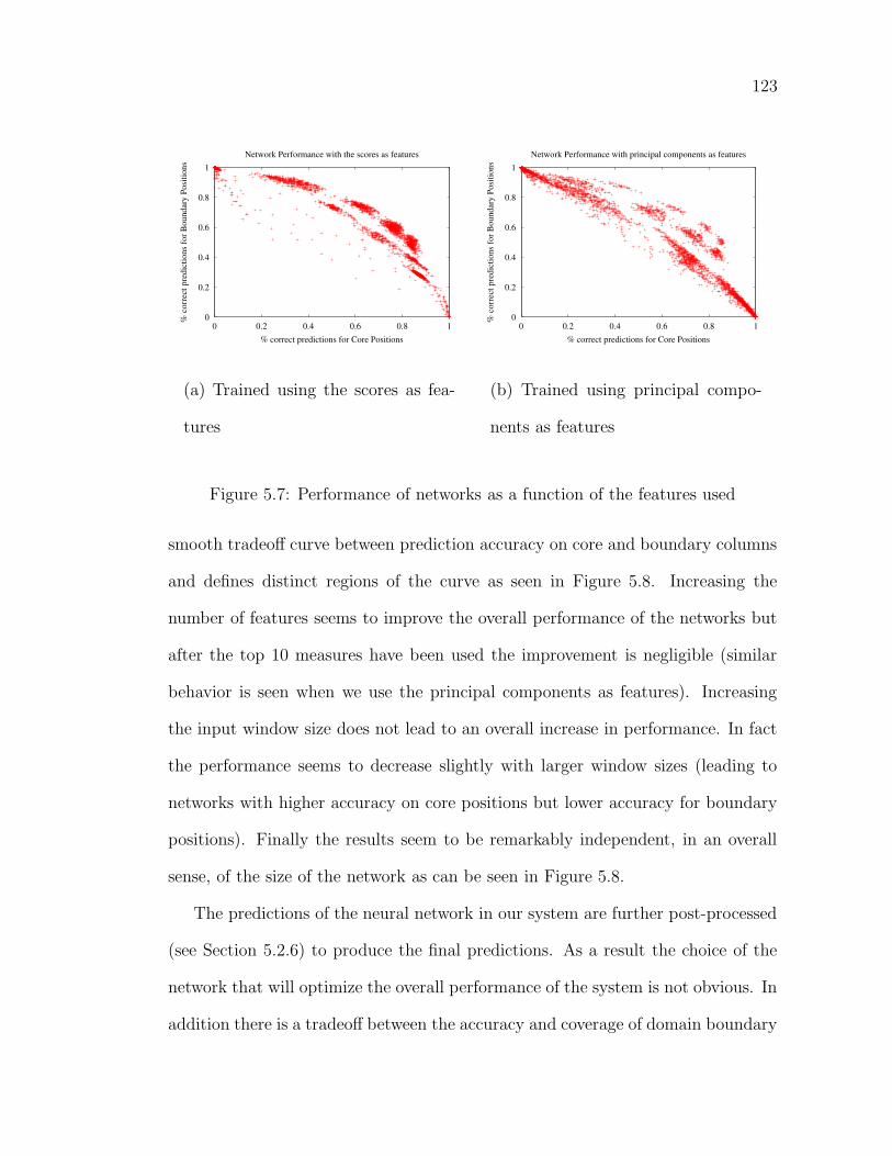
123
0
0.2
0.4
0.6
0.8
1
0 0.2 0.4 0.6 0.8 1
% c
orre
ct p
redi
ctio
ns fo
r Bou
ndar
y Po
sitio
ns
% correct predictions for Core Positions
Network Performance with the scores as features
(a) Trained using the scores as fea-
tures
0
0.2
0.4
0.6
0.8
1
0 0.2 0.4 0.6 0.8 1
% c
orre
ct p
redi
ctio
ns fo
r Bou
ndar
y Po
sitio
ns
% correct predictions for Core Positions
Network Performance with principal components as features
(b) Trained using principal compo-
nents as features
Figure 5.7: Performance of networks as a function of the features used
smooth tradeoff curve between prediction accuracy on core and boundary columns
and defines distinct regions of the curve as seen in Figure 5.8. Increasing the
number of features seems to improve the overall performance of the networks but
after the top 10 measures have been used the improvement is negligible (similar
behavior is seen when we use the principal components as features). Increasing
the input window size does not lead to an overall increase in performance. In fact
the performance seems to decrease slightly with larger window sizes (leading to
networks with higher accuracy on core positions but lower accuracy for boundary
positions). Finally the results seem to be remarkably independent, in an overall
sense, of the size of the network as can be seen in Figure 5.8.
The predictions of the neural network in our system are further post-processed
(see Section 5.2.6) to produce the final predictions. As a result the choice of the
network that will optimize the overall performance of the system is not obvious. In
addition there is a tradeoff between the accuracy and coverage of domain boundary

124
0
0.2
0.4
0.6
0.8
1
0 0.2 0.4 0.6 0.8 1
% c
orre
ct p
redi
ctio
ns fo
r Bou
ndar
y Po
sitio
ns
% correct predictions for Core Positions
Effect of varying core to boundary ratio
0.40.81.21.6
(a) Ratio of core to boundary
columns
0
0.2
0.4
0.6
0.8
1
0 0.2 0.4 0.6 0.8 1
% c
orre
ct p
redi
ctio
ns fo
r Bou
ndar
y Po
sitio
ns% correct predictions for Core Positions
Effect of varying the number of measures
124
1022
(b) Number of features
0
0.2
0.4
0.6
0.8
1
0 0.2 0.4 0.6 0.8 1
% c
orre
ct p
redi
ctio
ns fo
r Bou
ndar
y Po
sitio
ns
% correct predictions for Core Positions
Effect of varying the input window size
15
17
(c) Input window size
0
0.2
0.4
0.6
0.8
1
0 0.2 0.4 0.6 0.8 1
% c
orre
ct p
redi
ctio
ns fo
r Bou
ndar
y Po
sitio
ns
% correct predictions for Core Positions
Effect of varying the network size
largemedium
small
(d) Network size
Figure 5.8: Performance of networks as a function of various parameters

125
predictions (see Section 5.3.) To resolve the question of which neural network
to use we start by pruning our set of networks to only those networks that are
not strictly dominated by any other network in terms of network performance
(this corresponds to the points on the outer boundary of the curve in Figure 5.7.)
Since the performance for the principle component based networks is similar to
the performance of the networks that use the scores as features, we retain only the
142 networks that are trained on the scores. Some of the representative points in
this set are presented in Table 5.5. We continue the discussion of the appropriate
network to choose in Section 5.3.
5.2.6 Hypothesis evaluation
The neural networks that we trained do not take into account the predictions for
neighboring positions (and for the protein as a whole) while making a prediction for
a position5. Thus, despite the high rate of accurate predictions for single positions,
the final predictions may overly fragment proteins into domains.
To refine the initial predictions of the neural-net the following three steps are
employed. First, to eliminate spurious transition points the curve is smoothed.
This way, a position is predicted as a candidate transition point only if a signifi-
cant fraction of the positions around it are predicted as transition points by the
neural network (this fraction can be altered as a threshold parameter to give differ-
ent levels of accuracy and sensitivity as is described in Section 5.3). Secondly, for
regions below the threshold all the minimas are predicted as candidate transition
points (see Figure 5.9). The third step is the most important one. Each possible
5attempts to learn the mapping from local neighborhoods in the input space tolocal neighborhoods in the output space failed to improve the performance

126
Table 5.5: A sample from the set of selected networks
Number of Input window Core-Boundary Size of Size of % correct % correct
features size ratio first layer second layer core predictions boundary positions
10 9 0.4 20 15 0.04 0.98
4 3 0.4 25 30 0.23 0.95
15 1 0.4 20 30 0.39 0.90
4 9 0.8 15 5 0.56 0.80
10 3 0.8 5 30 0.63 0.76
15 1 0.8 30 25 0.70 0.70
22 3 1.6 25 5 0.81 0.57
10 5 1.6 5 10 0.88 0.43
2 17 1.6 5 30 0.91 0.30
7 5 0.4 25 30 0.96 0.20
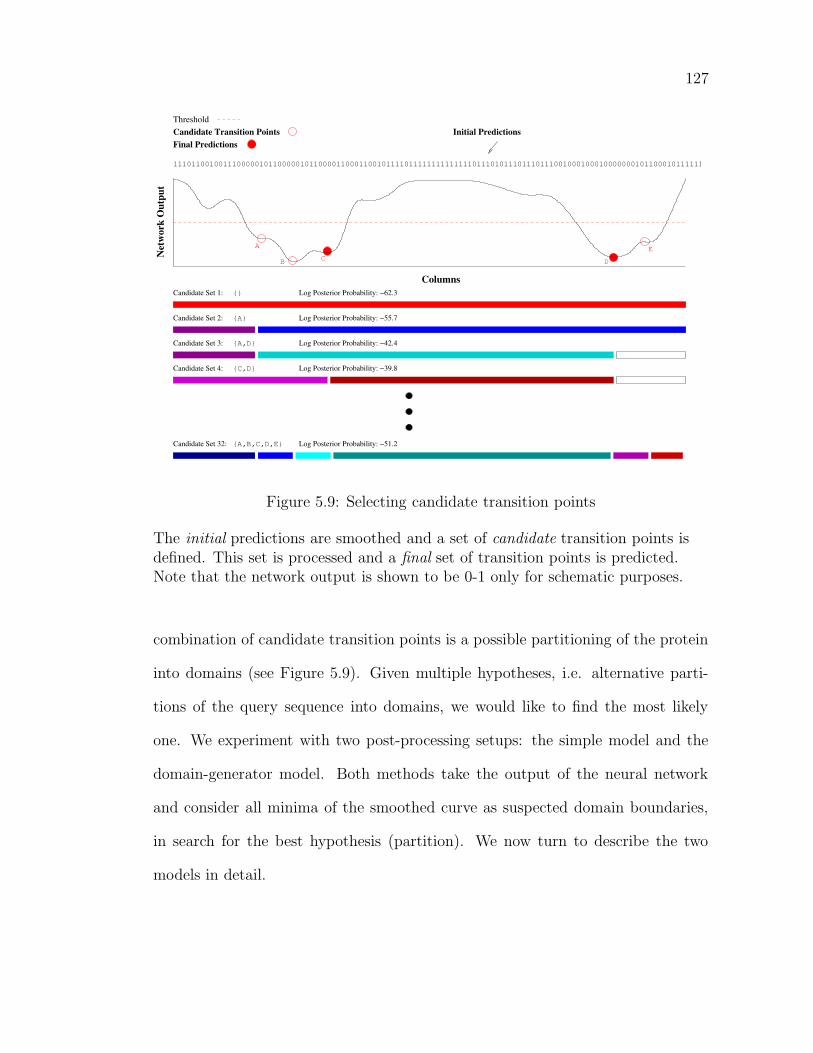
127
Net
wor
k O
utpu
t
Columns
Threshold
A
B CE
D
Candidate Set 1:
Candidate Set 2:
Candidate Set 3:
Candidate Set 4:
Candidate Set 32: {A,B,C,D,E}
{C,D}
{A,D}
{A}
{}
Log Posterior Probability: −51.2
Log Posterior Probability: −39.8
Log Posterior Probability: −42.4
Log Posterior Probability: −55.7
Log Posterior Probability: −62.3
111011001001110000010110000010110000110001100101111011111111111111011101011101110111001000100010000000101100010111111
Initial PredictionsCandidate Transition PointsFinal Predictions
Figure 5.9: Selecting candidate transition points
The initial predictions are smoothed and a set of candidate transition points isdefined. This set is processed and a final set of transition points is predicted.Note that the network output is shown to be 0-1 only for schematic purposes.
combination of candidate transition points is a possible partitioning of the protein
into domains (see Figure 5.9). Given multiple hypotheses, i.e. alternative parti-
tions of the query sequence into domains, we would like to find the most likely
one. We experiment with two post-processing setups: the simple model and the
domain-generator model. Both methods take the output of the neural network
and consider all minima of the smoothed curve as suspected domain boundaries,
in search for the best hypothesis (partition). We now turn to describe the two
models in detail.

128
5.2.6.1 The domain-generator model
The domain-generator model assumes a random generator that moves repeatedly
between a domain state and a linker state and emits one domain or transition at a
time according to different source probability distributions. Thus the probability
of a sequence of domains is given by the product of domain-emission probabilities
and the transition probabilities
Formally, we are given a protein sequence and a multiple alignment S of length
L and a possible partition D of S into n domains D = D1, D2, . . . , Dn of lengths
l1, l2, . . . , ln (as suggested by the output of the neural-net). Our goal is to find the
most likely model, i.e. the partition that maximizes the posterior probability of the
model given the data P (D|S). Our algorithm enumerates all possible combinations
of these positions and the one that maximizes the posterior probability is selected.
Note that while this could be computationally expensive, for most proteins the
number of candidate transition points is less than 15 (as is the case for all proteins
in our test set) thus making this process feasible.
To compute the posterior probability we first estimate the prior and the likeli-
hood of the data given the partition P (S|D), based on the precalculated measures
described in Section 5.2.2. By Bayes formula we can then estimate the posterior
probability
P (D|S) =P (S|D)P (D)
P (S)
The denominator is fixed for all hypotheses and so we are looking for the partition
that will maximize the product of the likelihood P (S|D) and the prior P (D)
Computing the prior: To calculate the prior P (D) we have to estimate the
probability that an arbitrary protein sequence of length L will consist of d domains

129
of the specific lengths l1, l2, . . . , ln. What we need to calculate then is
P (D) = P ((D1, l1)(D2, l2) . . . (Dn, ln) s.t. l1 + l2 + ..+ ln = L)
This can be estimated from the data by considering known domain partitions of
proteins of length L. However, the amount of data available is not enough to
accurately estimate these probabilities for all possible partitions. We approximate
this probability by using a simplified model; given the length of the protein, the
generator selects the number of domains first and then selects the length of one
domain at a time, considering the domains that were already generated. For
a partition into n domains there are n! possible orderings of the domains and
therefore the prior probability of the partition is approximated by
P (D) ' Prob(n|L) ·∑
π(l1,l2,...,ln)
P0(l1|L)P0(l2|L− l1)
. . . P0(ln−1|L−n−2∑
1
li)
where Prob(n|L) is the prior probability that a sequence of length L constitutes of
n domains and P0(li|L) is the prior probability to emit a domain of length li given
a sequence of length L. The term π(l1, l2, . . . , ln) denotes all possible permutations
of l1, l2, . . . , ln.
The prior probabilities P0(li|L) are approximated by P0(li), normalized to the
relevant range [0..L], and are estimated from the empirical distribution of domain
lengths in the SCOP database6. The empirical distribution is very noisy, sparse
for domains longer than 600 amino acids and biased due to uneven sampling of the
protein space, even after eliminating redundancy (see Figure 5.10a). To overcome
6Ideally, we would like to use P0(li|L). However, the SCOP data set is very noisyand the resulting distributions are heavily biased towards the domain definitionsin SCOP.

130
0
0.005
0.01
0.015
0.02
0 200 400 600 800 1000
Prob
abili
ty
Length
Distribution of domain lengths
originalunbiased
(a) Before and after eliminating bias.
0
0.0005
0.001
0.0015
0.002
0.0025
0.003
0.0035
0.004
0.0045
0.005
0 200 400 600 800 1000
Prob
abili
ty
Length
Distribution of domain lengths
empiricalEVD
(b) After smoothing.
Figure 5.10: Distributions of domain lengths

131
the bias we retain only one entry of the same length from each protein family
(Figure 5.10a). Noise and sparse sampling for domains longer than 600 amino acids
are handled by running a few smoothing cycles that resulted in the distribution
plotted in Figure 5.10b. Interestingly, the obtained distribution follows closely the
extreme value distribution (see Section 5.3.6 for discussion).
The second term, Prob(n|L) is given by Prob(n|L) = Prob(n, L)|P (L) where
Prob(n, L) is estimated by the (n− 1)th order sum
Prob(n, L) =
L∑
1
P0(x1)
L∑
1
P0(x2) . . .
L∑
1
P0(xn−1) · P0(L− x1 − x2 − · · · − xn−1)
and P (L) is simply given by the complete probability formula
P (L) =L∑
i=i
Prob(i, L)
The extrapolated distributions for n = 1..7 are plotted in Figure 5.11a. It should be
noted that the empirical distributions differ quite markedly from these extrapolated
distributions (Figure 5.11b). However, since the data is noisy, sparse and possibly
biased, we consider the extrapolated distributions to be more reliable than the
empirical ones. For one, note that the empirical probability for a protein to be a
single domain dominates all other scenarios up to proteins of length 400(!), while
the curves meet much earlier (around 200) in the extrapolated distributions. Our
observation is also supported by the quite different distributions observed in the
CATH database, further deprecating the reliability of the empirical distributions.
The impact of the extrapolated distributions is indeed evident in our results (see
Section 5.3). Our model tends to predict more domains than SCOP, and in many
cases refines SCOP partitions into more compact substructures.

132
0
0.2
0.4
0.6
0.8
1
0 200 400 600 800 1000 1200 1400
Prob
abili
ty
Length
Distribution of domain complexity (number of domains)
1 domain2 domains3 domains4 domains5 domains6 domains7 domains
(a) Extrapolated
0
0.2
0.4
0.6
0.8
1
0 100 200 300 400 500 600 700
Prob
abili
ty
Length
Distribution of domain complexity (number of domains)
1 domain2 domains3 domains4 domains
(b) Empirical
Figure 5.11: Distributions of number of domains
The extrapolated distributions are normalized assuming that the maximalnumber of domains is 7 (the maximal number of domains observed in SCOP). Inour calculations we considered up to 20 domains. These probabilities can beprecalculated using a dynamic programming algorithm.

133
Computing the likelihood: To calculate the likelihood of the data given the
model P (S|D) we use the probabilities of the observed scores given the domain
structure as predicted by the neural-net. We consider the individual domains
and the transitions between domains (the linkers) as two different sources. Each
source induces a unique probability distribution over the domain-information con-
tent scores (see Section 5.2.2). Specifically, given the model D that partitions the
sequence S into n domains and n− 1 transitions D1, T1, D2, T2, . . . , Tn−1, Dn that
correspond to the subsequences s1, t1, s2, t2, . . . , tn−1, sn we estimate the likelihood
by
P (S|D) = P (S|D1, T1, D2, Tn−1, Dn)
= P (s1|D1)P (t1|T1)P (s2|D2) ·
P (t2|T2) . . . P (tn−1|Tn−1)P (sn|Dn)
where we already employed the assumption that the domains are independent of
each other (see Section 5.2.6.3 for discussion). Each one of the terms P (si|Di) and
P (tj|Tj) is a product over the probabilities of the individual positions. The proba-
bility on an individual position j in domain i is estimated by the joint probability
distribution of the k features that are used in our system
P (sij|Di) = P (f1, f2, . . . , fk|Di)
However, estimating this probability is impractical given the amount of data we
have. On the other hand, given the correlation between scores (see Section 5.3.2)
the independence assumption for the individual scores does not hold. Therefore
we adopt an intermediate approach. We start by writing the exact formulation of
the joint probability distribution of k random variables X1, X2, . . . , Xk using the
134
expansion
P (X1, X2, .., Xk) = P (X1)P (X2|X1)P (X3/X1, X2)
. . . P (Xk|X1, X2, .., Xk−1)
where the random variables can be ordered in an arbitrary order. We then derive an
approximation to these probabilities using first-order dependencies7 and a heuristic
expansion. The methodology is as follows: for each pair of random variables X, Y
we calculate the distance between the joint probability distribution and the product
of the marginal probability distributions
DEPEN(X, Y ) ≡ Dist(PXY , PXPY )
This distance (measured either using the l1 norm or the JS divergence measure) is
a measure of the dependency between the two variables. The larger it is, the more
dependent are the variables (one might also consider using the mutual information
measure instead).
We sort all pairs based on their distance and pick the most dependent one first
(denoted by Y1 and Y2) to start the expansion
P (X1, X2, .., Xk) = P (Y1)P (Y2|Y1) . . . . . .
The next terms are selected based on their strongest dependency with variables
that are already used in the expansion. Thus
Y3 = arg maxY{max{DEPEN(Y, Y1), DEPEN(Y, Y2)}}
Denote by Z = PILLAR(Y ) the random variable that Y is most dependent on
(of the random variables that are already in the expansion), then of all possible
7Pair statistics can be calculated quite reliably from our data set, but the datais too sparse to derive reliable estimates of higher order statistics

135
dependencies involving Y3 we pick P (Y3|PILLAR(Y3)) and add it to the expansion
P (X1, X2, .., Xk) = P (Y1)P (Y2|Y1) · P (Y3|PILLAR(Y3)) . . . . . .
The procedure continues until all variables are accounted for. This heuristic at-
tempts to minimize the errors that are introduced by relaxing the dependency as-
sumption to a first order dependency by maximizing the support for each random
variable we introduce in the expansion. Thus, highly correlated variables affect the
total probability only marginally, while under the independence assumption they
might introduce a substantial error (other, alternative methods for approximat-
ing the joint probability distribution from the marginal distributions are described
in [Ireland & Kullback 1968] and [Pearl 1997]). Note that the expansion for do-
main regions can be different from the expansion for linker regions, as the source
distributions differ.
However, once the two expansions (for domains and linkers) are defined based
on the pair statistics, the same two expansions are used for all domains and all
linkers.
Hypothesis selection: Given a set of N candidate transition points (the minimas
of the neural network output), our algorithm enumerates all possible combinations
of transition points to form 2N possible partitions (hypotheses). For each partition
we calculate the posterior probability (using our domain-generator model) and
eventually output the most likely one. The whole calculation is very fast. For
example, for a protein of length L = 300 and a set of N = 10 possible transition
points, the algorithm will output the most probable hypothesis in a matter of
minutes.

136
5.2.6.2 The simple model
In the simple model, the candidate transition points are listed in decreasing order of
reliability (as measured by the depth of the corresponding minima in the smoothed
curve) and considered in this order. Once a minima is selected all minima that are
within a window of k amino acids around it are rejected (where k is a function of
the protein length). This is a greedy approach that seems to work pretty well for
many proteins. The depth of the minima is a good approximation of the overall
posterior probability of the transition points P (Ti|ti), as the network essentially
assigns a value O(i) that indicates the network’s confidence in this position as being
an in-domain position. Thus 1−O(i) (the depth of the minima) is the probability
that this position is a boundary position.
5.2.6.3 The independence index
Both our models explicitly or implicitly assume that the domains across transition
points are independent. However, when searching for the best model one should
also consider the validity of this assumption and the “quality” of the predicted
transition points. Not only should they indicate domain boundaries, but they
should also justify the independence assumption over neighboring domains that
we employed above.
We define the following confidence or independence index for each transition
point. This index estimates the likelihood that the domains on both sides of the
transition point are independent of each other. This likelihood is estimated as
follows: if indeed the two domains were formed independently then the patterns of
sequence divergence should be different. By comparing the divergence patterns one
can indirectly measure the statistical similarity of the sources that generated the

137
two domains. The divergence pattern is given by the distribution of evolutionary
distances of sequences in the alignment of each domain (using the subset of n
common sequences). For each sequence we approximate its evolutionary distance
from the query seed sequence by counting the number of point mutations per
100 amino acids. The specific divergence pattern (the vector of n − 1 distances)
is a reflection of the statistical source that generated the domain. To quantify
the likelihood that the source distributions are unique we compute the pearson
correlation between the two divergence patterns and this gives us our independence
index. Zero correlation indicates two unique sources (independent domains).
To assess the quality of each individual transition point we compute the in-
dependence index, and report its statistical significance in terms of its z-score
(computed based on the background distribution of independence indices over a
large set of randomly selected positions). These numbers are reported for each
transition point in the final prediction. Thus, the user can evaluate not only the
plausibility of the overall partition but also of each individual transition. For com-
parison, the average independence index for random positions is 0.79 (standard
deviation of 0.26), while for true transition points the average is 0.68 (standard
deviation of 0.34). In other words, true transition points partition proteins into
less correlated domains, as desired.
5.3 Results
To test our approach we run our system on a subset of 460 proteins that were
excluded from the training set. The test set was well balanced in terms of the
number of multi-domain proteins with 222 single domain and 238 multi-domain
proteins (of which 179 are two-domain, 43 are three-domain, 13 are four-domain
138
and 3 are five-domain proteins). For each of these proteins the prediction was
compared to that of SMART [Ponting et al. 1999], Tigr [Haft et al. 2001], Pfam
[Bateman et al. 1999] and ProDom [Sonnhammer & Kahn 1994], based on the in-
formation provided by InterPro [Apweiler et al. 2001] as well as predictions from
DOMO [Gracy & Argos 1998] obtained by running BLAST searches against the
DOMO database. Interpro predictions for ProDom are limited to a curated subset
of ProDom and so we also present results predicted directly by ProDom for pro-
teins in the test set that can be matched (based on their accession numbers) to
the complete ProDom database.
Since the predictions obtained from other systems are often incomplete for the
seed proteins in our test set, we needed to design an evaluation procedure that
would have different scores for accuracy and coverage. In addition, the predictions
may disagree with SCOP on the number of domains in the seed protein. Therefore
one needs to define a procedure for associating predicted transition points with
their most probable SCOP counterparts and vice versa. The simplest choice is
to assign every transition point that is being considered to the closest reference
transition point. Here we adopt this model and define the following four measures:
Distance accuracy. This measure evaluates predictions by using SCOP transi-
tion points as reference. For each seed protein we calculate the average distance of
the predicted transitions from their associated SCOP transition points. The final
value that is reported is the average distance over all proteins in the test set.
Distance sensitivity. This measure assesses the sensitivity in detecting true
domain boundaries by using the predicted transitions as reference. The average
distance of SCOP transitions from the associated predicted transitions is calculated
for each protein, with the value reported being the average of this distance over
139
all proteins in the test set.
Selectivity. For this measure we consider predictions that are within x = 10
residues of a SCOP transition as being correct with the final value reported being
the percentage of predictions that are considered correct for the entire set.
Coverage. Analogous to accuracy, SCOP transitions that are associated with
a predicted transition point within x = 10 residues are considered successfully
predicted. The percentage of correctly predicted SCOP transitions for the entire
set is reported.
Using these measures we evaluated the results of post-processing the network
output for the final set of 142 optimal networks (see Section 5.2.5) using both the
simple model and the domain-generator model. As can be seen in Figure 5.12,
even though the performance of none of these networks dominates that of the
other, the performance after post-processing may do so. We also observe various
tradeoffs for selectivity vs. coverage based on which network we use. The choice of
which network to use should depend on the application that we have in mind (and
therefore the tradeoff that we would like to work with). For example, application
of this method for structural genomics purposes might require high selectivity to
avoid fragments that cannot fold independently. On the other hand domain family
classification programs may prefer high coverage to generate accurate sub-domain
families that can then be merged to get the final domain families. For the purpose
of evaluation we chose a single network for each model, as described in Figure 5.12.
The tradeoff curves in Figure 5.12 are not very smooth and changing the trade-
off requires us to change the network and the inputs used. This setup is therefore
not amenable for the construction of a flexible system where we can easily move
on the tradeoff curve. We can however get a smooth tradeoff curve similar to that

140
0
0.1
0.2
0.3
0.4
0.5
0.6
0 0.1 0.2 0.3 0.4 0.5 0.6
Cove
rage
Selectivity
Results for the final set of Networks
simple model
(a) Post-processing with simple model
0
0.1
0.2
0.3
0.4
0.5
0.6
0 0.1 0.2 0.3 0.4 0.5 0.6
Cove
rage
Selectivity
Results for the final set of Networks
domain-generator model
(b) Post-processing with domain-generator
Figure 5.12: Coverage vs. Selectivity for final set of networks
For each model we select a single network to work with, marked with a box.These networks are selected such that no other network dominates them. Theyare located at the cusps of a sudden fall in performance. Interestingly, both thesepoints correspond to the same network that uses all the 22 features, an inputwindow size of 1, core-boundary ratio of 1.6 and with hidden layers of size 25 and5 respectively.

141
0
0.1
0.2
0.3
0.4
0.5
0.6
0.7
0.1 0.2 0.3 0.4 0.5 0.6 0.7 0.8
Cove
rage
Selectivity
Tradeoff curve for a network
HMMPfamHMMSmart
HMMTigrBlastProDom
BlastDomodomain-generator model
simple model
Figure 5.13: Coverage vs. Selectivity tradeoff while varying the threshold
seen in Figure 5.13, for any fixed network that we choose, by varying the threshold
parameter (see Section 5.2.6) for the network ouput. This gives us the flexibility
of changing the performance of the system by altering a single parameter. The
curves seen in Figure 5.13 both have gentle cusps towards the top of the curves.
Both these points correspond to a threshold of 0.5. The results reported next are
obtained when setting the threshold parameter to that value.
First we evaluated our two post-processing methods. The results are sum-
marized in Table 5.6. Both methods perform almost the same, as measured by
the four performance indices described above. Nevertheless, the domain-generator
model has some advantages over the simple model. First, as opposed to the greedy
approach of the simple model, the domain-generator model considers all possi-
ble hypotheses. Moreover, it provides us with a critical statistical framework for
assessing alternative, competing hypotheses. The model can be used to assign
a confidence value to each hypothesis and by comparing these confidence values
(between the best hypothesis and the next best hypothesis or the set of all other

142
Table 5.6: Performance evaluation results for the two post-processing methods
Number of Accuracy/ Selectivity/
Predictions Sensitivity Coverage
(in residues) (percentages)
simple model 460 40/24 35/45
domain-generator 460 48/19 27/51
The number of predictions is the total number of proteins in the test set forwhich predictions were made. For each protein several transition points may bepredicted. Performance measures (accuracy, sensitivity, selectivity and coverage)are based on the complete set of predicted transition points.
hypotheses) one can define a significance measure and associate it with the out-
put hypothesis. In cases where the differences between competing hypotheses are
insignificant, one might also want to consider the alternative domain partitions.
A summary of the evaluation results for our method and other sequence based
methods is presented in Table 5.7. Our method significantly improved over all
other automatic methods, outperformed only by the manually calibrated Pfam
(see next section for discussion). Note that the criterion used to compute the
coverage and selectivity is very strict (the agreement must be within 10 residues).
One can relax this criterion by increasing the window size. This would result in
a 5-10% increase in performance for both measures when using a window of 15
residues, for example.
We also evaluated the overall consistency of the different methods. Specifically,
we ask how many proteins are predicted correctly completely, both in terms of the
total number of domains, and their exact locations. The results are summarized
in Table 5.8. Again, our method performed well compared to all other automatic

143
Table 5.7: Performance evaluation results for sequence based methods
Number of Accuracy/ Selectivity/
Predictions Sensitivity Coverage
(in residues) (percentages)
Our method 460 40/24 35/45
HMMPfam 441 29/14 43/65
BlastDomo 252 17/70 22/12
BlastProDom (Complete) 218 29/45 19/27
HMMSmart 172 12/73 27/17
BlastProDom (Interpro) 123 8/90 30/6
HMMTigr 51 2/96 33/1
The relatively good accuracy values for HMMTigr, ProDom, HMMSmart andDomo are the result of the small number of predictions these methods make. Theselectivity and coverage values are more indicative of the overall performance ofeach method.

144
methods. Moreover, while other methods performed well mostly over single domain
proteins, our method performs well on many multiple domain proteins as well.
5.3.1 Inclusion of structural information in prediction
When evaluating the results one has to keep in mind that incorporation of struc-
tural information, when available, can improve the quality of predictions. Indeed,
the PFam database uses this information explicitly by defining domains using the
SCOP database. It is not surprising therefore, that the manually calibrated PFam
performed better on the test set. Their performance, however, may not be as good
over an independent data set. In order to correct this bias, one would ideally like
to generate a totally independent test set. However, since Pfam is in the process
of integrating all of SCOP definitions to determine their domain definitions it is
hard or almost impossible to generate such a set.
Instead, we tested the effect of incorporation of structural information on our
predictions. We repeated the process, this time including the SCOP sequences
in the database. Thus the alignments that we generate might contain SCOP
amino acid sequences of structural domains. However, these sequences are not
used arbitrarily in our system to chop the proteins into domains. Rather, they
add to the overall signal in each one of the constituent measures and it is the
cumulative contribution that is detected by our learning system. As a result, both
sequences of unknown structures and sequences of known structures can affect
the predictions. In other words, our learning system does not explicitly use the
structural information and it processes alignments that contain SCOP sequences
exactly the same way it processes alignments which are based purely on sequences
of unknown structures. The results of this procedure are summarized in Tables

145
Table 5.8: Global consistency results
Number Correct number Number of completely Correct predictions Correct predictions
predictions of domains correct predictions (single domain) (multi-domain)
Our method 460 267 205 134 71 (35%)
HMMPfam 441 309 276 178 98 (36%)
BlastDomo 252 148 118 98 20 (17%)
BlastProDom (C) 218 94 83 51 32 (39%)
HMMSmart 172 112 91 70 21 (23%)
BlastProDom (I) 123 83 75 63 12 (16%)
HMMTigr 51 23 21 20 1 (5%)
The two results for ProDom are those obtained using the complete definitions (C) and the interpro subset (I). Thepercentages in the last column are the percentages of correct predictions of multi-domain proteins out of all correctpredictions. Among the multi-domain proteins the percentages of correctly predicted two-domain proteins, three-domainproteins etc. remain roughly the same as their proportions in the test set.

146
Table 5.9: Performance evaluation results when structural information is used
Number of Accuracy/ Selectivity/
Predictions Sensitivity Coverage
(in residues) (percentages)
Our method 460 27/6 63/83
HMMPfam 441 29/14 43/65
PFam explicitly uses the structural information available from SCOP domains.To test the effect of these sequences on the predictions we included them in thealignments, and used those alignments as input for our system. Thus, under thissetup, our system uses the structural information implicitly.
Table 5.10: Global consistency results when structural information is used
Number Correct number Number of completely
predictions of domains correct predictions
Our method 460 318 308
HMMPfam 441 309 276
5.9 and 5.10. Note the significant improvement in performance for our method.
Especially notable are the significant coverage and selectivity.
5.3.2 Examples
The overall performance of our method shows that the model is capable of learning
even subtle signals that indicate domain boundaries. Our first example is a three
domain protein that was predicted accurately for all its domains. This is the PDB
protein 1qpb (chain B), 563 residues long. The protein is partitioned by SCOP
into three domains that correspond to positions 2-181, 182-360 and 361-556. Our

147
prediction suggests transition points at positions 181 and 354 (see Figure 5.14)
within 6 residues from SCOP definitions. These positions are correlated with
strong combined termination and insertion entropy signals. In addition there is
an abundance of proline residues around positions 180 and 360 and there are class
entropy spikes around positions 110, 180, 360 and 500. For comparison, PFam
predicts three thiamine pyrophosphate enzyme domains at positions 2-180, 197-
348 and 361-538. No predictions were available from ProDom, DOMO, SMART
or Tigr.
Another example where our method correctly predicted all the domain transi-
tion points is for the protein 1g8h (chain B). However, in this case none of the other
sequence-based predictions (including PFam) were able to partition the protein cor-
rectly. This protein is 511 amino acids long and according to SCOP it consists
of three independent domains, between positions 2-168, 169-389 and 390-511 (see
Figure 5.15). Our prediction locates domain boundaries at positions 165 and 392,
within three residues from the SCOP definition. In PDB, 1gh8 is annotated as
an archaeal translation elongation factor. However a HMM search using PFam
reports the main domain being an ATP-sulfurylase between positions 72-392. A
look at the structure of the protein clearly shows that this is an unsatisfactory
domain definition. Similarly Prodom (Interpro) predicts a domain between posi-
tions 37 and 393. Both Domo and Tigr make similar predictions (1-396 and 4-386)
that merge the first and second domains into one large domain. No predictions are
available from SMART. Detailed analysis of our system in this case reveals com-
bined termination signals at positions 80, 180, 290 and 390 and weighted mutation
profile troughs at positions 120 and 390. Peaks in insertion entropy are also seen
at positions 140, 160 and 250 and an abundance of proline residues is seen around
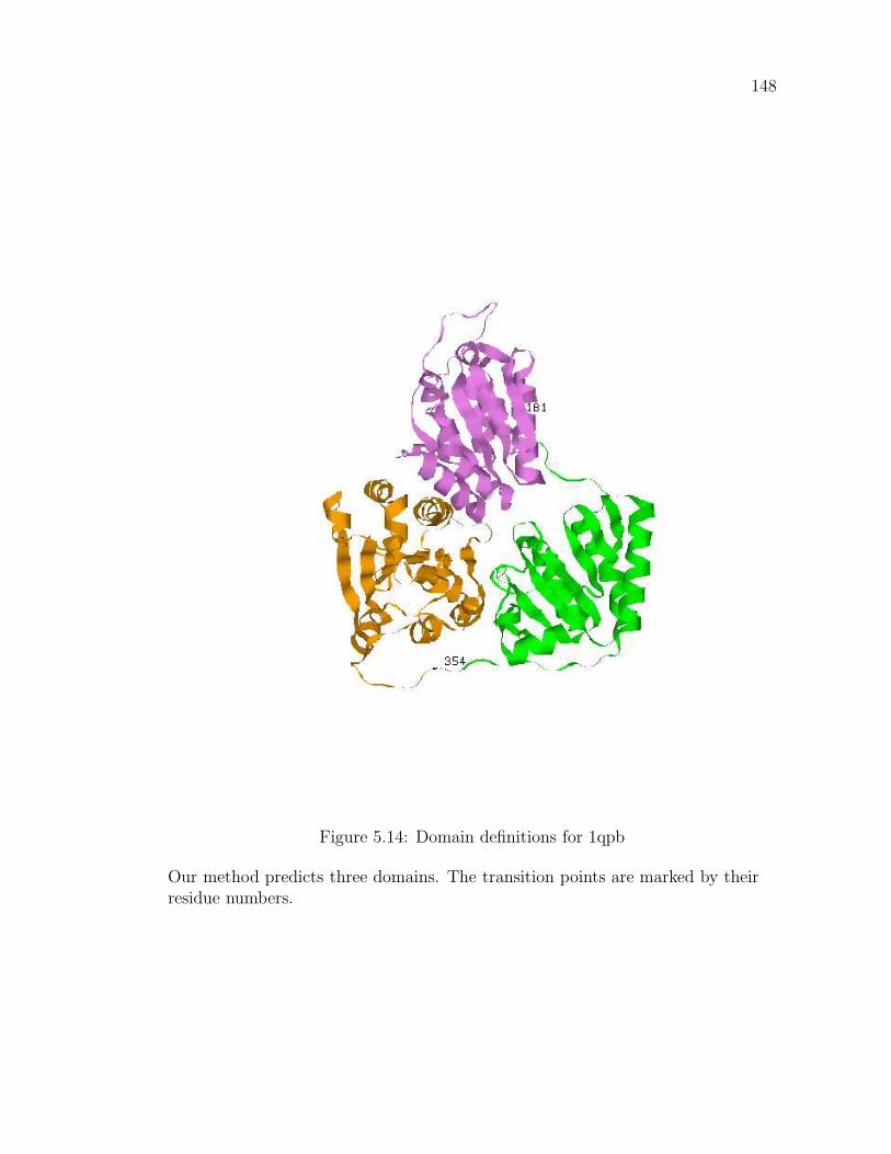
148
Figure 5.14: Domain definitions for 1qpb
Our method predicts three domains. The transition points are marked by theirresidue numbers.

149
positions 260 and 390.
5.3.3 Suggested novel partitions
The list of proteins on which our method failed to correctly predict domain bound-
aries as defined by SCOP revealed interesting cases. Many of them raise serious
questions about the validity of SCOP definitions. For example, PDB protein 1acc
(735 amino acids long) is defined as a single domain in SCOP. Our analysis suggests
three domains at positions 1-160, 161-586 and 587-735 (see Figure 5.16). As the
figure illustrates, this partition seems to better satisfy the definition of a domain as
a compact, independent foldable unit. Moreover, given the distribution of domain
sizes in proteins (see Section 5.2.6.1), it is not very likely to have protein domains
that are longer than 700 amino acids, thus further supporting our hypothesis. For
comparison, Pfam detects one domain at positions 103-544 (PF03495 Clostridial
Binary exotoxin B) and Domo predicts two domains at positions 1-647 and 648-735.
No predictions are available from ProDom (Interpro), SMART or Tigr.
In this case we get a clean and strong joint termination signal at positions 160
and 590, and a remarkably consistent alignment between positions 170 and 580.
This signal is reinforced by other measures: the hydrophobic curve has three major
troughs at 170, 290 and 570, insertion entropy has major peaks at 180, 310 and
560 and correlation is pretty low around 200, 280 and 590.
Another interesting example is the PDB protein 1ffv (chain E) that is 803
residues long and partitioned by SCOP into two domains defined by the positions
7-146 and 147-803. Our method predicts four domains at positions 1-141, 142-426,
427-591 and 592-803 (see Figure 5.17). While our prediction agrees with SCOP in
defining the first domain, it further partitions the second domain into three sub-

150
Figure 5.15: Domain definitions for 1gh8
In this case a mosaic of signals (combined termination, weighted mutation profile,insertion entropy and proline) is integrated by our system into two predictions(three domains) that are in good agreement with SCOP’s structural definition.

151
Figure 5.16: Domain definitions for 1acc
SCOP define this protein as a single domain. Our analysis suggests threecompact units.

152
units. Analysis of the protein structure indicates that the second domain predicted
by our method does defines a distinct, reasonably compact structural domain. In
addition while the third and fourth domains are intertwined in space, there seems
to be a clear symmetry in their construction suggesting the possibility that they
arose as a result of duplication. Interestingly, CATH also partitions the protein
into four domains though the definitions are much more complicated (domain1:
7-141 and 210-306, domain2: 142-209 and 307-383, domain3: 484-649, domain4:
440-483 and 650-803). The signals that our method gets for predicting the addi-
tional domain boundaries at positions 426 and 591 are quite strong. In addition to
a strong neural-network output we also observe strong sequence termination and
class entropy signals around all three positions.
In both cases, SCOP definitions might be inaccurate because of the lack of
structural information to support the existence of these domains. SCOP domains
are defined as recurrent structural subunits and in the absence of other copies of
these domains the proteins are left untouched. Our analysis indicates that had
the structures of related proteins been resolved such evidence would have become
available. In the presence of such strong signals based on sequence information
it is clear that the domain structure of proteins cannot be determined based on
structural information alone.
5.3.4 Analysis of errors
Our method does fail in cases where signals are misleading. This usually seems to
happen when the domain definition for the protein is complicated by the unusual
structure and topology of the protein. One such case is for the beta-barrel protein
1qkc. It is classified by SCOP as a single domain protein while our method predicts

153
Figure 5.17: Domain definitions for 1ffv
Our analysis of this protein helps us to identify two likely domain boundariesthat are missed by SCOP and that help partition the protein into more compactdomains (domains are rotated for visual clarity).
154
three domains defined by the positions 1-256, 257-394, 395-725 (see Figure 5.18).
In comparison PFam predicts a domain between positions 615 and 725 and Domo
predicts two domains at positions 21-337 and 338-725. In general, beta-barrel pro-
teins are considered hard test cases, even for structural domain classifiers. While
our predictions clash with the standard definition of classifying the entire barrel
structure as one domain it is interesting to note that both boundary predictions
made by our method are in looped regions, even though it is much more likely
that a prediction lies in a beta strand region (based on the beta to loop ratio). In
addition, while it is not clear if the domains predicted by our method are the cor-
rect pieces, it seems quite plausible that the beta-barrel structure evolved by the
fusion of two or more barrel pieces. The domain boundary predicted by DOMO
also lends some support to our prediction. Further investigation from a biological
perspective of the pieces that we identify as domains may help prove or disprove
this hypothesis.
Another unusual case is the PDB protein 1i6v that is 1118 residues long. SCOP
classifies this protein as a single domain protein. Our method partitions the protein
into four domains defined by the positions 1-220, 221-513, 514-830 and 831-1118
(see Figure 5.19). As can be seen from the rasmol ribbons image, this protein is
highly unstructured and has a complicated topology. The domains defined by our
method do not partition the protein into clean, structurally distinct units. However
they do indicate that 1i6v is probably not a single domain protein. Our predictions
are supported by significant confidence index values (see Section 5.2.6.3) as well.
The length of the protein is another factor that suggests that this protein is multi-
domain. It is possible that some of the domains in 1i6v are non-continuous, further
complicating domain prediction.

155
Figure 5.18: Domain definitions for 1qkc
Example of a beta-barrel protein where our method predicts component domainsthat need further investigation in order to be validated.

156
Figure 5.19: Domain definitions for 1i6v
We believe that many of the “errors” will be resolved as more structures are
solved and SCOP definitions are refined. In some cases, the situation wil require a
more precise definition of what a domain is. Finally, increase in sequence data and
design of more sophisticated measures employing additional sources of information
will help to improve predictions.
5.3.5 Consistency of domain predictions
Our gold standard so far was the SCOP database of protein domains. The domains
in this database are defined manually based on visual inspection of protein struc-
tures, however, there is no assurance that the definitions are indeed accurate and
correspond to the “true” definitions. Since no quantitative rules or principles are
used, different points of view might lead to somewhat different domain definitions.
To assess the stability and accuracy of our domain prediction algorithm we
tested it on CATH [Orengo et al. 1997] which is another structure-based domain
classification system. CATH combines sequence analysis with structure comparison

157
Table 5.11: Performance evaluation results using domain definitions in CATH
Number of Accuracy/ Selectivity/
Predictions Sensitivity Coverage
(in residues) (percentages)
SCOP 220 14/13 74/76
simple model 220 37/27 34/42
domain-generator model 220 46/23 27/47
HMMPfam 209 32/24 36/52
BlastDomo 125 17/65 24/14
BlastProDom (Complete) 104 32/48 15/23
HMMSmart 80 11/75 22/12
BlastProDom (Interpro) 62 8/86 31/7
HMMTigr 22 3/92 20/1
algorithms to determine structural domains. Of the 238 multi-domain proteins in
our test set we were able to map 158 proteins to release 2.4 of CATH8. Of the
222 single domain proteins in the test set we were able to map almost all (217)
to CATH. Of the 158 multi-domain proteins, 48 contained discontinuous domains
(according to CATH) that cannot be predicted with our method (see discussion
below) and therefore were eliminated. To keep the numbers of single and multi-
domain proteins balanced we sampled 110 proteins from the list of single domain
proteins to get a new test set of 220 proteins.
8Based on the PDB identifiers we were able to map most of the proteins (197 outof 238), but since CATH uses the ATOMRES records while we use the SEQRESrecords of the PDB files, there were some discrepancies (gaps, and length mismatchbetween ATOMRES and SEQRES records) that deemed some files unusable fortesting.

158
We repeated our performance evaluations over this set of 220 proteins using
the CATH definitions as the standard of truth. The results are given in Table
5.11. As can be seen from the first line of the table, while CATH and SCOP are
in pretty good agreement they do differ in some cases. Based on comparison with
the results in Table 5.7 we can see that the performance of our method is stable
across CATH and SCOP. The stability of our results therefore indicates that our
methodology learns a more general concept of domains. In contrast, we see that
the performance of PFam on CATH is not as good as on SCOP. This could be
explained by the fact that PFam definitions are often guided by SCOP definitions.
We studied example cases where our predictions were different from those of
CATH. We found that in general in such cases CATH differs from our method (as
well from SCOP) because of its tendency to assign small structural fragments from
one sequence domain to another based on structural compactness considerations.
An example of such a situation is the protein 1ekx (chain A) that is 311 residues
long. SCOP defines two domains, the first one between positions 2-151 and the
second between positions 152-311 (see Figure 5.20). Our method predicts one
transition point at position 151, in excellent agreement with the SCOP definition.
The predictions from PFam (8-150, 153-305) and Prodom (7-150, 157-306) also
agree with this definition. CATH defines the first domain as a combination of
two fragments 1-133 and 292-310 and a second domain at positions 134-291. This
results in a fragment of an alpha helix being assigned to the first domain based on
compactness considerations alone.
The inconsistency with our method is not surprising, as our definition of a
domain is evolutionary motivated. Our model assumes that protein domains are
ancient and evolutionary conserved sequence fragments that have emerged as pro-

159
Figure 5.20: Domain definitions for 1ekx
The differently colored segments on the top left and bottom right define the twodomains of the protein. CATH assigns the fragment between positions 292-310(in blue) to the domain on the top while our method and SCOP assign it to thedomain on the bottom.

160
tein building blocks during evolution. This does not cover all possible domain
definitions. Multiple studies showed that in practice the structural arrangement of
proteins can form compact substructures that are sequence discontinuous. How-
ever, such sequence discontinuous domains need accurate structural information to
delineate them correctly, and it is not clear if it is possible to detect these domains
based on sequence information alone. In the absence of clear evolutionary evidence
supporting this assignment, it is also not clear how to translate such definitions to
our domain definitions. Moreover, the signals, if they exist, might be different from
those for continuous domains, and to learn these signals would require designing
a different learning system. These issues make the identification of discontinuous
domains a harder and possibly orthogonal problem to the one that we tried to
solve in this study.
5.3.6 The distribution of domain lengths
We were intrigued by the fact that the distribution of domain lengths follows
closely the extreme value distribution (EVD), as in Figure 5.10b. This distribu-
tion has been studied extensively, in particular in the context of sequence similarity
[Karlin & Altschul 1990, Dembo & Karlin 1991] and has been used by packages
such as BLAST [Altschul et al. 1997] and FASTA [Pearson & Lipman 1988] to as-
sociate statistical significance measures (E-values) with similarity scores. However,
its appearance in the context of domain lengths is surprising and deserves further
study.

161
5.4 Discussion
In this chapter we presented a novel method for detecting the domain structure of
a protein from sequence information alone. Our method utilizes the information
in sequence databases and starts by comparing the query sequence with all the
sequences in the database. The search generates a multiple alignment and the
alignment is processed fully automatically in search for domain transition signals.
There are several novel elements in our method. First, our method uses multi-
ple scores. Some of the scores we designed are variations on measures that were
suggested in earlier studies (e.g sequence participation and correlation scores were
used in DOMO, ProDom and PASS and correlated mutations were used in Rig-
den’s work). However, we introduce many novel scores based on the analysis of
basic sequence properties or predicted properties, scores that are calculated from
multiple alignments and scores that are extracted from external resources such
as intron-exon data. Secondly, we use information theory principles to optimize
the scores and select the subset that maximizes the domain information content.
Thirdly, a neural network is trained to learn a non-linear mapping from the original
scores to a single output. Finally, a probabilistic domain-generator model is devel-
oped to assess multiple hypotheses and predict the most likely one. Unlike local or
heuristic methods that employ a greedy search through the hypothesis space, our
model exhaustively enumerates all possible partitions of the protein into domains,
until it finds the optimal one. This multi-stage system is not only robust to align-
ment inaccuracies, but it can also tolerate partial information. It can be extended
and generalized to include other types of scores. Most importantly, our method
suggests for the first time a rigorous model that can test all possible hypotheses
and output the one that is most consistent with the data. We also developed an

162
evaluation framework that hopefully will provide a clearer understanding of the
strengths and weaknesses of the algorithms that have been designed so far and thus
aid in the design of better algorithms. Moreover, our domain-generator model can
associate a statistical significance score for every hypothesis, thus enabling us to
compare different hypotheses by the same method or even different hypotheses by
several different methods.
We trained and tested our method on what is considered to be the gold stan-
dard in protein structure classification, the SCOP database of protein domains.
Our method performed very well compared to all other methods currently available
while being fully automatic. One should keep in mind that SCOP is a man-made
classification and the definitions of domains do not necessarily conform with “na-
ture’s definitions”. Indeed many of our supposedly errors seem to make sense when
inspected visually. Moreover, SCOP might be inaccurate near domain boundaries,
as the selection of the actual transition point is quite arbitrary. Our method pro-
vides a rigorous and accurate way to predict not only the domain structure but also
the most likely transition points and can be used to augment or guide predictions
based on structural data.
The utility of our tool goes beyond simple structural analysis of proteins. It
can help in predicting the complete 3D structure of a protein, as the task can be
divided into smaller tasks, given the predicted domain structure of the protein. It
can have significant impact on structural genomics efforts. The high throughput
structural determination of proteins is more likely to succeed when the proteins are
broken into smaller, structurally stable units. Using our model to predict domain
boundaries can help in that aspect too. Finally, it is essential for the study of
proteins’ building blocks and for functional analysis.

163
There are several variations to the model described here that we consider intro-
ducing in the future. Although our algorithm is not overly sensitive to alignment
accuracy, obviously better multiple alignment algorithms are expected to improve
the performance. Since the system uses the domain-generator model to process
hypotheses, it is less sensitive to the exact details of the learning system, however,
replacing the neural network with another learning system (such as SVMs) might
also improve performance slightly. Another possible improvement is the integra-
tion of a weighting scheme into the multiple alignment. Currently all sequences
are weighted equally. However, due to the biased representation of protein families
in sequence databases and the nature of sequence comparison algorithms, diverged
sequences that might provide us with crucial information about domain bound-
aries are usually underrepresented in these alignments. To eliminate this bias one
should decrease the weight of highly similar sequences and increase the weight of
highly diverged sequences. Preliminary attempts in that direction (implementing
the schema described in [Henikoff & Henikoff 1994]) did not show a significant im-
provement, however the results are not conclusive. Hopefully these variations will
further fine-tune the performance of our system.
Finally, our method can be easily extended to include structural information to
aid in the process of domain prediction. All it takes is to include these sequences
in the alignment. If the learning system recognizes a strong signal (e.g. sequence
termination) that is consistent with other sequences of unknown structure, a pre-
diction will be made that is in agreement with the structural information. This
approach can help in unifying manual expert-based approaches with more rigor-
ous information-content based methods, to produce more reliable predictions of
domains.

164
5.5 Acknowledgements
This work was done in collaboration with and under the guidance of Dr. Golan
Yona.

165
BIBLIOGRAPHY
[Murvai et al. 2001] Murvai, J., Vlahovicek, K., Szepesvari, C. & Pongor, S.(2001). Prediction of Protein Functional Domains from Sequences Using Ar-tificial Neural Networks. Genome Res. 11, 1410-1417.
[Miyazaki et al. 2002] Miyazaki, S., Kuroda, Y. & Yokoyama, S. (2002). Char-acterization and prediction of linker sequences of multi-domain proteins by aneural network J. Structural and Functional Genomics 15, 37-51.
[Altschul et al. 1997] Altschul, S. F., Madden, T. L., Schaffer, A. A., Zhang, J.,Zhang, Z., Miller, W. & Lipman, D.J. (1997). Gapped BLAST and PSI-BLAST:a new generation of protein database search programs. Nucl. Acids Res. 25,3389-3402.
[Apweiler et al. 2001] Apweiler, R. et al. (2001). The InterPro database, an in-tegrated documentation resource for protein families, domains and functionalsites. Nucl. Acids Res. 29, 37-40.
[Bairoch & Apweiler 1999] Bairoch, A. & Apweiler, R. (1999). The SWISS-PROTprotein sequence data bank and its supplement TrEMBL in 1999. Nucl. AcidsRes. 27 49-54.
[Bateman et al. 1999] Bateman, A., Birney, E., Durbin, R., Eddy, S. R., Finn R.D., & Sonnhammer E. L. (1999). Pfam 3.1: 1313 multiple alignments and profileHMMs match the majority of proteins. Nucl. Acids Res. 27, 260-262.
[Black & Mould 1991] Black, S.D. & Mould, D.R. (1991). Development of Hy-drophobicity Parameters to Analyze Proteins Which Bear Post or Cotransla-tional Modifications. Anal. Biochem. 193, 72-82.
[Csiszr] Csiszr, I. Information Theoretic Methods in Probability and Statistics.From citeseer.nj.nec.com
[Dembo & Karlin 1991] Dembo, A. & Karlin, S. (1991). Strong limit theorems ofempirical functionals for large exceedances of partial sums of i.i.d variables. Ann.Prob. 19, 1737-1755.
[Ferran et al. 1994] Ferran, E. A., Pflugfelder, B. & Ferrara P. (1994). Self-Organized Neural Maps of Human Protein Sequences. Protein Sci. 3, 507-521.
[George & Heringa 2002] George, R. A. & Heringa, J. (2002). Protein domainidentification and improved sequence similarity searching using PSI-BLAST.Proteins 48, 672-681.

166
[George & Heringa 2002] George, R. A. & Heringa, J. (2002). SnapDRAGON: amethod to delineate protein structural domains from sequence data. J. Mol.Biol. 316, 839-851.
[George et al. 1996] George, D. G., Barker, W. C., Mewes, H. W., Pfeiffer, F.& Tsugita, A. (1996). The PIR-International protein sequence database. Nucl.Acids. Res. 24, 17-20.
[Gilbert & Glynias 1993] Gilbert, W. & Glynias, M. (1993). On the ancient natureof introns. Gene 135, 137-144.
[Gilbert et al. 1997] Gilbert, W., de Souza, S. J. & Long, M. (1997). Origin ofgenes. Proc. Natl Acad. Sci. USA 94, 7698-7703.
[Gouzy et al. 1999] Gouzy, J., Corpet, F. & Kahn, D. (1999). Whole genome pro-tein domain analysis using a new method for domain clustering. Comput Chem.23, 333-340.
[Gracy & Argos 1998] Gracy, J. & Argos, P. (1998). Automated protein sequencedatabase classification. I. Integration of copositional similarity search, local sim-ilarity search and multiple sequence alignment. II. Delineation of domain bound-ries from sequence similarity. Bioinformatics 14:2, 164-187.
[Guan & Du 1998] Guan, X. & Du, L. (1998). Domain identification by clusteringsequence alignments. Bioinformatics 14, 783-788.
[Ireland & Kullback 1968] Ireland, C. T. & Kullback, S. (1968). Contingency ta-bles with given marginals. Biometrika 55, 179-189.
[Haft et al. 2001] Haft, D. H., Loftus, B. J., Richardson, D. L., Yang, F., Eisen, J.A., Paulsen, I. T. & White, O. (2001). TIGRFAMs: a protein family resourcefor the functional identification of proteins. Nucl. Acids Res. 29, 41-43.
[Henikoff & Henikoff 1992] Henikoff, S. & Henikoff, J. G. (1992). Amino acid sub-stitution matrices from protein blocks. Proc. Natl Acad. Sci. USA 89, 10915-10919.
[Henikoff & Henikoff 1994] Henikoff, S. & Henikoff, J.G. (1994). Position-basedsequence weights. J. Mol. Biol. 243, 574-578.
[Henikoff & Henikoff 1996] Henikoff, J. G. & Henikoff, S. (1996). Using substi-tution probabilities to improve position-specific scoring matrices. Comp. App.Biosci. 12:2, 135-143.
[Holm & Sander 1994] Holm, L. & Sander, C. (1994). Parser for protein foldingunits. Proteins 19, 256-268.

167
[Hubbard et al. 1999] Hubbard, T. J., Ailey, B., Brenner, S. E., Murzin, A. G.& Chothia, C. (1999). SCOP: a Structural Classification of Proteins database.Nucl. Acids Res. 27, 254-256.
[Karlin & Altschul 1990] Karlin, S. & Altschul, S. F. (1990). Methods for assessingthe statistical significance of molecular sequence features by using general scoringschemes. Proc. Natl Acad. Sci. USA 87, 2264-2268.
[Kullback 1959] Kullback, S. (1959). ”Information theory and statistics”. JohnWiley and Sons, New York.
[Kuroda et al. 2000] Kuroda, Y., Tani, K., Matsuo, Y. & Yokoyama, S. (2000).Automated search of natively folded protein fragments for high-throughputstructure determination in structural genomics. Protein Sci. 9, 2313-2321.
[Lesk & Rose 1981] Lesk, A. M. & Rose, G. D. (1981). Folding units in globularproteins. Proc. Natl. Acad. Sci. USA 78, 4304-4308.
[Lin 1991] Lin, J. (1991). Divergence measures based on the Shannon entropy.IEEE Trans. Info. Theory 37:1, 145-151.
[McGuffin et al. 2000] McGuffin, L. J. , Bryson, K. & Jones, D. T. (2000). ThePSIPRED protein structure prediction server. Bioinformatics 16, 404-405.
[Murzin et al. 1995] Murzin, A. G., Brenner, S. E., Hubbard, T. & Chothia, C.(1995). SCOP: a structural classification of proteins database for the investiga-tion of sequences and structures. J. Mol. Biol. 247, 536-540.
[Orengo et al. 1997] Orengo, C. A., Michie, A. D., Jones, S., Jones, D. T.,Swindells, M. B. & Thornton, J. M. (1997). CATH-a hierarchic classificationof protein domain structures. Structure 5, 1093-1108.
[Park & Teichmann 1998] Park, J. & Teichmann, S. A. (1998). DIVCLUS: an au-tomatic method in the GEANFAMMER package that finds homologous domainsin single- and multi-domain proteins. Bioinformatics 14:2, 144-150.
[Pazos et al. 1997] Pazos, F., Helmer-Citterich, M., Ausiello, G. & Valencia, A.(1997). Correlated mutations contain information about protein-protein inter-action. J. Mol. Biol. 271, 511-523.
[Pearl 1997] Pearl, J. (1997). ”Probabilistic Reasoning in Intelligent Systems: Net-works of Plausible Inference.” Morgan Kaufmann Publishers Inc., San Mateo,California.
[Pearson & Lipman 1988] Pearson, W. R. & Lipman, D. J. (1988). Improved toolsfor biological sequence comparison. Proc. Natl. Acad. Sci. USA 85, 2444-2448.

168
[Ponting et al. 1999] Ponting, C. P., Schultz, J., Milpetz, F. & Bork, P. (1999).SMART: identification and annotation of domains from signalling and extracel-lular protein sequences. Nucl. Acids Res. 27, 229-232.
[Rigden 2002] Rigden, D. J. (2002). Use of covariance analysis for the prediction ofstructural domain boundaries from multiple protein sequence alignments. Pro-tein Eng. 15, 65-77.
[Rose 1979] Rose, G. D. (1979). Hierarchic organization of domains in globularproteins. J. Mol. Biol. 134, 447-470.
[Saxonov et al. 2000] Saxonov, S. , Daizadeh, I. , Fedorov, A. & Gilbert, W.(2000). EID: the Exon-Intron Database-an exhaustive database of protein-codingintron-containing genes. Nucl. Acids Res. 28, 185-190.
[Sonnhammer & Kahn 1994] Sonnhammer, E. L. L. & Kahn, D. (1994). Modulararrangement of proteins as inferred from analysis of homology. Protein Sci. 3,482-492.
[Sonnhammer et al. 1997] Sonnhammer, E. L., Eddy, S. R., Durbin, R. (1997).Pfam: a comprehensive database of protein domain families based on seed align-ments. Proteins 28, 405-420.
[Sowdhamini & Blundell 1995] Sowdhamini, R. & Blundell, T. L. (1995). An au-tomatic method involving cluster analysis of secondary structures for the iden-tification of domains in proteins. Protein Sci. 4, 506-520.
[Taylor 1999] Taylor, W. R. (1999). Protein structural domain identification. Pro-tein Eng. 12, 203-216.
[Westbrook et al. 2002] Westbrook, J., Feng, Z., Jain, S. et al. (2002). The ProteinData Bank: unifying the archive. Nucl. Acids. Res. 30, 245-248
[Wheelan et al. 2000] Wheelan, S. J., Marchler-Bauer, A. & Bryant, S. H. (2000).Domain size distributions can predict domain boundaries. Bioinformatics 16,613-618.
[Yona & Levitt 2000b] Yona, G. & Levitt, M. (2000). Towards a complete mapof the protein space based on a unified sequence and structure analysis of allknown proteins. In the proceedings of ISMB 2000, 395-406, AAAI press, MenloPark.
[Yona et al. 1999] Yona, G., Linial, N. & Linial, M. (1999). ProtoMap: Automaticclassification of protein sequences, a hierarchy of protein families, and local mapsof the protein space. Proteins, 37, 360-378.

CHAPTER 6
FUTURE WORK
6.1 Extensions to the bagFFT algorithm
While the bagFFT algorithm is asymptotically the fastest known algorithm for
computing the p-value of the G2 statistic it can be slower than Hirji’s algorithm
for small n and K. A possible improvement to bagFFT to remedy this can be
based on the csFFT technique described in Chapter 3. Also, extending bagFFT
for Pearson’s X2 statistic and for log-linear models, as well as a generalization to
two-column contingency tables are natural directions for future research in this
area [Baglivo et al., 1992].
6.2 Alignment significance in alternate models
An important assumption used in sFFT and csFFT is that alignment columns are
independently generated under the null hypothesis. This assumption is however
typically not borne out in genomic DNA that we would consider “random” (non-
coding sequences far away from regulatory regions). To correct for this many motif
finders use a higher-order markov model for the null-hypothesis [Liu et al., 2001,
Thijs et al., 2001, Bailey and Elkan, 1994]. The significance of the motif is then
evaluated by sampling from the distribution of motif scores obtained by the motif
finder on random sequences from the null model. The sampling process is however
very slow (it requires a call to the motif finder for every sample) and is not suitable
for the kind of optimization we do in Chapter 4. Extending the techniques in
Chapter 3 or designing new algorithms for this problem is an interesting open
problem.
169

170
Two related problems where techniques similar to those in Chapter 3 may
apply occur in the motif scanning problem. Here the motif model is known and
we wish to scan genomic DNA to find significant matches. While there exist
efficient solutions when the columns of the motif are independent, solving the
problem in the important case where motif columns are correlated is still an open
problem. With the availability of multiple genomes, recent work has explored the
use of phylogenetic models to simultaneously search for motif matches upstream of
orthologous genes [Moses et al., 2004]. The question of efficiently estimating the
significance of motifs under these phylogenetic models is also an interesting avenue
for future research.
6.3 Improvements to Conspv and Gibbspv
The motif finders in Chapter 4 were restricted to the assumption that every se-
quence has exactly one occurence of the motif of interest. This is however an
unrealistic assumption and in practice input sequences may have 0 or multiple
occurences of the motif. We hope to explore ideas similar to those in Chapter 4 in
this more general framework as part of our future work.
6.4 Improved protein domain delineation
In recent years there have been several studies on the subject of domain delineation
[Kim et al., 2005, Tanaka et al., 2006, Miyazaki et al., 2006, Liu and Rost, 2004,
Sim et al., 2005, Dumontier et al., 2005, Gewehr and Zimmer, 2006] and some of
them have followed our framework of using neural networks to analyze multiple
alignments for predicting protein domains [Liu and Rost, 2004, Sim et al., 2005].

171
While these methods typically report performance improvements over first genera-
tion tools such as Prodom, on an absolute scale the results are still unsatisfactory
and far from the goal of reliable domain delineation that is important for tasks such
as protein classification and predicting domain interactions. We believe that the
next generation of tools can be develped based on a combination of the following
ideas:
• Constructing multiple alignments in conjunction with domain delineation:
The method described in Chapter 5 currently works by constructing a multi-
ple alignment and then using the alignment to delineate domains. However,
the alignment process itself could greatly benefit from knowledge of where
the domain boundaries are. In the present setup, errors in the multiple-
alignment could propagate to errors in domain delineation, with no scope for
correction of the alignment in the presence of conflicting information from
the domain delineation step. Two obvious solutions that could work are:
1. Iteratively use the domain definitions from our method to improve the
multiple alignment and then use the new multiple alignment to get new
domain definitions till the process converges.
2. Modify the scoring scheme in a progressive multiple alignment tool to
use domain delineation signals (such as the output form the neural
network in our method) from subalignments.
• Phylogenetic analysis of alignment columns: An important source of infor-
mation that is missing in the analysis done in our method is the evolutionary
tree that connects the sequences in the multiple alignment. For many of our
scores taking the phylogeny into account would be valuable to weight the

172
information obtained from various sequences. Typically, however, the phy-
logeny of the sequences in our alignments in unknown and we would need to
infer it computationally. While this is a difficult problem in itself, techniques
to integrate over phylogenies can help us cope with the uncertainity in the
phylogeny [Jin et al., 2006, Kosiol et al., 2006].
• Learning multiple models: Bagging and Boosting are two commmonly used
techniques in machine learning to improve the performance of a classifier
[Schwenk and Bengio, 2000]. These techniques could also be valuable in our
method if it is indeed the case that different domain families have different
sets of rules that define their domain boundaries.

173
BIBLIOGRAPHY
[Baglivo et al., 1992] Baglivo,J., Olivier,D. and Pagano,M. (1992) Methods for ex-act goodness-of-fit tests. Journal of the American Statistical Association, 87(418), 464–469.
[Bailey and Elkan, 1994] Bailey,T.L. and Elkan,C. (1994) Fitting a mixture modelby expectation maximization to discover motifs in biopolymers. Proc Int ConfIntell Syst Mol Biol, 2, 28–36.
[Dumontier et al., 2005] Dumontier,M., Yao,R., Feldman,H.J. and Hogue,C.W.V.(2005) Armadillo: domain boundary prediction by amino acid composition. JMol Biol, 350 (5), 1061–1073.
[Gewehr and Zimmer, 2006] Gewehr,J.E. and Zimmer,R. (2006) SSEP-Domain:protein domain prediction by alignment of secondary structure elements andprofiles. Bioinformatics, 22 (2), 181–187.
[Jin et al., 2006] Jin,G., Nakhleh,L., Snir,S. and Tuller,T. (2006) Inferring Phylo-genetic Networks by the Maximum Parsimony Criterion: A Case Study. MolBiol Evol.
[Kim et al., 2005] Kim,D.E., Chivian,D., Malmstrm,L. and Baker,D. (2005) Au-tomated prediction of domain boundaries in CASP6 targets using Ginzu andRosettaDOM. Proteins, 61 Suppl 7, 193–200.
[Kosiol et al., 2006] Kosiol,C., Bofkin,L. and Whelan,S. (2006) Phylogenetics bylikelihood: evolutionary modeling as a tool for understanding the genome. JBiomed Inform, 39 (1), 51–61.
[Liu and Rost, 2004] Liu,J. and Rost,B. (2004) Sequence-based prediction of pro-tein domains. Nucleic Acids Res, 32 (12), 3522–3530.
[Liu et al., 2001] Liu,X., Brutlag,D.L. and Liu,J.S. (2001) BioProspector: discov-ering conserved DNA motifs in upstream regulatory regions of co-expressedgenes. Pac Symp Biocomput, 127–138.
[Miyazaki et al., 2006] Miyazaki,S., Kuroda,Y. and Yokoyama,S. (2006) Identifi-cation of putative domain linkers by a neural network - application to a largesequence database. BMC Bioinformatics, 7, 323.
[Moses et al., 2004] Moses,A.M., Chiang,D.Y., Pollard,D.A., Iyer,V.N. andEisen,M.B. (2004) MONKEY: identifying conserved transcription-factor bind-ing sites in multiple alignments using a binding site-specific evolutionary model.Genome Biol, 5 (12), R98.

174
[Schwenk and Bengio, 2000] Schwenk,H. and Bengio,Y. (2000) Boosting neuralnetworks. Neural Comput, 12 (8), 1869–1887.
[Sim et al., 2005] Sim,J., Kim,S.Y. and Lee,J. (2005) PPRODO: prediction of pro-tein domain boundaries using neural networks. Proteins, 59 (3), 627–632.
[Tanaka et al., 2006] Tanaka,T., Yokoyama,S. and Kuroda,Y. (2006) Improvementof domain linker prediction by incorporating loop-length-dependent characteris-tics. Biopolymers, 84 (2), 161–168.
[Thijs et al., 2001] Thijs,G., Lescot,M., Marchal,K., Rombauts,S., Moor,B.D.,Rouz,P. and Moreau,Y. (2001) A higher-order background model improves thedetection of promoter regulatory elements by Gibbs sampling. Bioinformatics,17 (12), 1113–1122.