Embed Size (px)
Citation preview

Statistical Thinking and SmartExperimental Design
Animal Experiments
Luc Wouters

Version 1.1 Copyright ©2017 Luc Woutershttp://www.luwo.behttp://www.datascope.be

Contents
1 Introduction 11.1 The problem with the biosciences . . 1
1.2 Structure of this text . . . . . . . . . 3
1.3 Software . . . . . . . . . . . . . . . . 4
2 Smart Research Design by StatisticalThinking 52.1 The architecture of experimental re-
search . . . . . . . . . . . . . . . . . . 5
2.1.1 The controlled experiment . . 5
2.1.2 Scientific research as aphased process . . . . . . . . 5
2.1.3 Scientific research as an iter-ative, dynamic process . . . . 6
2.2 Research styles - The smart researcher 6
2.3 Principles of statistical thinking . . . 7
3 Planning the Experiment 93.1 The planning process . . . . . . . . . 9
3.2 Types of experiments . . . . . . . . . 10
3.3 The pilot study . . . . . . . . . . . . 11
4 Principles of Statistical Design 134.1 Some terminology . . . . . . . . . . . 13
4.2 The structure of the response variable 13
4.3 Defining the experimental unit . . . 13
4.4 Variation is omnipresent . . . . . . . 15
4.5 Balancing internal and external va-lidity . . . . . . . . . . . . . . . . . . 16
4.6 Bias and variability . . . . . . . . . . 16
4.7 Requirements for a good experiment 17
4.8 Strategies for minimizing bias andmaximizing signal-to-noise ratio . . 18
4.8.1 Strategies for minimizingbias - good experimentalpractice . . . . . . . . . . . . . 18
4.8.1.1 The use of controls . 18
4.8.1.2 Blinding . . . . . . . 19
4.8.1.3 The presence of atechnical protocol . 19
4.8.1.4 Calibration . . . . . 20
4.8.1.5 Randomization . . . 20
4.8.1.6 Random sampling . 22
4.8.1.7 Standardization . . 22
4.8.2 Strategies for controllingvariability - good experi-mental design . . . . . . . . . 22
4.8.2.1 Replication . . . . . 22
4.8.2.2 Subsampling . . . . 23
4.8.2.3 Blocking . . . . . . . 24
4.8.2.4 Covariates . . . . . 24
4.9 Simplicity of design . . . . . . . . . . 25
4.10 The calculation of uncertainty . . . . 25
5 Common Designs in Biological Experi-mentation 275.1 Error-control designs . . . . . . . . . 28
5.1.1 The completely randomizeddesign . . . . . . . . . . . . . 28
5.1.2 The randomized completeblock design . . . . . . . . . . 29
5.1.2.1 The paired design . 30
5.1.2.2 Efficiency of therandomized com-plete block design . 30
5.1.3 Incomplete block designs . . 32
5.1.4 Latin square designs . . . . . 33
5.1.5 Incomplete Latin square de-signs . . . . . . . . . . . . . . 34
5.2 Treatment designs . . . . . . . . . . . 35
5.2.1 One-way layout . . . . . . . . 35
5.2.2 Factorial designs . . . . . . . 35
5.3 More complex designs . . . . . . . . 40
5.3.1 Split-plot designs . . . . . . . 40
5.3.2 The repeated measures design 41
5.3.3 The crossover design . . . . . 42
i

ii CONTENTS
6 The Required Number of Replicates -Sample Size 456.1 The need for sample size determina-
tion . . . . . . . . . . . . . . . . . . . 45
6.2 Determining sample size is a risk -cost assessment . . . . . . . . . . . . 45
6.3 The context of biomedical experiments 45
6.4 The hypothesis testing context - thepopulation model . . . . . . . . . . . 46
6.5 Sample size estimation . . . . . . . . 47
6.5.1 Power based calculations . . 47
6.5.2 Mead’s resource require-ment equation . . . . . . . . . 50
6.6 How many subsamples . . . . . . . . 50
6.7 Multiplicity and sample size . . . . . 52
6.8 The problem with underpoweredstudies . . . . . . . . . . . . . . . . . 53
6.9 Sequential plans . . . . . . . . . . . . 54
7 The Statistical Analysis 577.1 The statistical triangle . . . . . . . . 57
7.2 The statistical model revisited . . . . 57
7.3 Significance tests . . . . . . . . . . . 58
7.4 Verifying the statistical assumptions 59
7.5 The meaning of the p-value and sta-tistical significance . . . . . . . . . . 59
7.6 Multiplicity . . . . . . . . . . . . . . 61
8 The Study Protocol 63
9 Interpretation and Reporting 659.1 The ARRIVE Guidelines . . . . . . . 65
9.1.1 Introduction section . . . . . 65
9.1.2 Methods section . . . . . . . 65
9.1.3 The Results section . . . . . . 66
9.2 Additional topics in reporting results 67
9.2.1 Graphical displays . . . . . . 67
9.2.1.1 Percentage of con-trol - A commonmisconception . . . 67
9.2.1.2 Interpreting andreporting signifi-cance tests . . . . . 68
10 Concluding Remarks and Summary 7110.1 Role of the statistician . . . . . . . . 71
10.2 Recommended reading . . . . . . . . 71
10.3 Summary . . . . . . . . . . . . . . . . 72
References 73
Appendices
Appendix A Glossary of Statistical Terms 81
Appendix B Introduction to R 85B.1 Installation . . . . . . . . . . . . . . . 85
B.2 Packages for experimental design . . 85
Appendix C Tools for randomization in MSExcel and R 87C.1 Completely randomized design . . . 87
C.1.1 MS Excel . . . . . . . . . . . . 87
C.1.2 R-Language . . . . . . . . . . 87
C.2 Randomized complete block design 88
C.2.1 MS Excel . . . . . . . . . . . . 88
C.2.2 R-Language . . . . . . . . . . 88
Appendix D ARRIVE Guidelines 89

1. Introduction
More often than not, we are unable to reproduce findings published by researchers in journals.
Glenn Begley, Vice President Research Amgen (2015)
The way we do our research [with our animals] is stone-age.
Ulrich Dirnagl, Charité University Medicine Berlin (2013)
1.1 The problem with the bio-
sciences
Over the past decade, the biosciences have beenplagued by problems with the replicability and re-producibility1 of research findings. This lack of re-liability can be attributed in large part to statisticalfallacies, misconceptions, and other methodolog-ical issues (Begley and Ioannidis, 2015; Loscalzo,2012; Peng, 2015; Prinz et al., 2011; Reinhart, 2015;van der Worp et al., 2010). The following exam-ples illustrate some of these problems and showthat there is a definite need to transform and im-prove the research process.
Example 1.1. In 2006, a research team from Duke Uni-
versity led by Anil Potti published a paper claiming
that they had built an algorithm using genomic microar-
ray data that allowed to predict which cancer patients
would respond to chemotherapy (Potti et al., 2006).
This would spare patients the side effects of ineffective
treatments. Of course, this paper drew a lot of attention
and many independent investigators tried to reproduce
the results. Keith Baggerly and Kevin Coombes, two
statisticians at MD Anderson Cancer Center, were also
asked to have a look at the data. What they found
was a mess of poorly conducted data analysis (Baggerly
and Coombes, 2009). Some of the data was mislabeled,
some samples were duplicated in the data, sometimes
samples were marked as both sensitive and resistant,
etc. Baggerly and Coombes concluded that they were
unable to reproduce the analysis carried out by Potti
et al. (2006), but the damage was done. Several clin-
ical trials had started based on the erroneous results.
In 2011, after several corrections, the original study by
Potti et al. was retracted from Nature Medicine, stat-
ing: ”because we have been unable to reproduce certain
crucial experiments” (Potti et al., 2011).
Example 1.2. In 2009, a group of researchers from Har-
vard Medical School published a study showing that
cancer tumors could be destroyed by targeting the
STK33 protein (Scholl et al., 2009). Scientists at Am-
gen Inc. pounced on the idea and assigned a team of 24
researchers to try to repeat the experiment with the ob-
jective of developing a new medicine. After six months
of intensive lab work, it turned out that the project
was a waste of time and money since it was impos-
sible for the Amgen scientists to replicate the results
(Babij et al., 2011; Naik, 2011). Unfortunately, this
was not the only problem of replicability the Amgen re-
searchers encountered. During a decade Begley and El-
lis (2012) identified a set of 53 “landmark” publications
in preclinical cancer research, i.e. papers in top journals
from reputable labs. A team of 100 scientists tried to
replicate the results. To their surprise, in 47 of the 53
studies (i.e. 89%) the findings could not be replicated.
This outcome was particularly disturbing since Begley
and Ellis did every effort to work in close collaboration
1Formally, we consider replicability as the replication of scientific findings using independent investigators, methods,data, equipment, and protocols. Replicability has long been and will continue to be the standard by which scientific claimsare evaluated. On the other hand, reproducibility means that starting from the data gathered by the scientist, we canreproduce the same results, p-values, confidence intervals, tables and figures as those reported by the scientist (Peng, 2009).
1
2 CHAPTER 1. INTRODUCTION
with the authors of the original papers and even tried
to replicate the experiments in the laboratory of the
original investigator. In some cases, 50 attempts were
made to reproduce the original data, without obtaining
the claimed result (Begley, 2012). What is even more
troubling is that Amgen’s findings were consistent with
those of others. In a similar setting, Bayer researchers
found that only 25% of the original findings in target
discovery could be validated (Prinz et al., 2011).
Example 1.3. Seralini et al. (2012) published a 2-year
feeding study in rats investigating the health effects of
genetically modified (GM) maize NK603 with and with-
out glyphosate-containing herbicides. The authors of
the study concluded that GM maize NK603 and low lev-
els of glyphosate herbicide formulations, at concentra-
tions well below officially-set safe limits, induce severe
adverse health effects, such as tumors, in rats. Apart
from the publication, Seralini also presented his findings
in a press conference, which was widely covered in the
media showing shocking photos of rats with enormous
tumors. Consequently, this study had a severe impact
on the general public and also on the interest of the
industry. The paper was used in the debate over a ref-
erendum over labeling of GM food in California, and it
led to bans on importation of certain GMOs in Russia
and Kenya. However, short after its publication many
scientists, among them also researchers from the VIB
(Vlaams Instituut voor Biotechnologie, 2012), heavily
criticized the study and expressed their concerns about
the validity of the findings. A polemic debate started
with opponents of GMOs and also within the scientific
community, which inspired media to refer to the contro-
versy as The Seralini affair or Seralini tumor-gate. Sub-
sequently, the European Food Safety Authority (2012)
thoroughly scrutinized the study and found that it was
of inadequate design, analysis, and reporting. Specifi-
cally, the number of animals was considered too small
and not sufficient for reaching a solid conclusion. Even-
tually, the journal retracted Seralini’s paper, claiming
that it did not reach the journal’s threshold of publica-
tion (Hayes, 2014) 1.
Example 1.4. Selwyn (1996) describes a study where
an investigator examined the effect of a test compound
on hepatocyte diameters. The experimenter decided to
study eight rats per treatment group, three different
lobes of each rat’s liver, five fields per lobe, and approx-
imately 1,000 to 2,000 cells per field. At that time, most
of the work, i.e. measuring the cell diameters, was done
manually, making the total amount of work, i.e. 15,000
- 30,000 measurements per rat, substantial. The exper-
imenter complained about the overwhelming amount of
work in this study and the tight deadlines that were set
up. A sample size evaluation conducted after the study
was completed indicated that sampling as few as 100
cells per lobe would have been without appreciable loss
of information.
Unreliable biological reagents and reference materials 36.1%
Improper studydesign 27.6%
Inadequatedata analysisand reporting 25.5%
Laboratory protocolerrors 10.8%
Figure 1.1 Categories of errors that contribute tothe problem of replicability in life science research(source Freedman et al. 2015)
Doing good science and producing high-quality data should be the concern of every se-rious research scientist. Unfortunately, as shownby the first three examples, this is not always thecase. As mentioned above, there is a genuine con-cern about the reproducibility of research findingsand it has been argued that most research find-ings are false (Ioannidis, 2005). In a recent paperBegley and Ioannidis (2015) estimated that 85% ofbiomedical research is wasted at large. Freedmanet al. (2015) tried to identify the root causes of thereplicability problem and to estimate its economicimpact. They estimated that in the United Statesalone approximately US$28B/year is spent on re-search that cannot be replicated. The main prob-lems causing this lack of replicability are summa-rized in Figure 1.1. Issues in study design anddata analysis accounted for more than 50% of thestudies that could not be replicated. Kilkenny et al.(2009), who surveyed 271 papers reporting labora-tory animal experiments found that many studieshad problems with the quality of reporting, qual-ity of experimental design, and quality of statisti-cal analysis. Most worrying was the fact that thequality of the experimental design in the majority
1Seralini managed to republish the study in Environmental Sciences Europe (Seralini et al., 2014), a journal with aconsiderably lower impact factor.

1.1. THE PROBLEM WITH THE BIOSCIENCES 3
of experiments was inappropriate or inefficient.
Not only scientists but also the journals have agreat responsibility in guarding the quality of theirpublications. Peer reviewers and editors, whohave little or no statistical training, let methodolog-ical errors pass undetected. Moreover, high-impactjournals tend to focus on statistically significant re-sults of unexpected findings, often without look-ing at the practical importance. Especially, in stud-ies with insufficient sample size, this publicationbias causes high numbers of false research claims.(Ioannidis, 2005; Reinhart, 2015).
In addition to the problem of replicability of re-search findings, there has also been a dramatic risein the number of journal retractions over the lastdecades (Cokol et al., 2008). In a review of all2,047 biomedical and life-science research articlesindexed by PubMed as retracted on May 3, 2012,Fang et al. (2012) found that 21.3% of the retrac-tions were due to error, while 67.4% of the retrac-tions were attributable to misconduct, includingfraud or suspected fraud (43.4%), duplicate pub-lication (14.2%), and plagiarism (9.8%).
Studies such as those by Potti et al. (2006), Schollet al. (2009), and Séralini et al. (2012), as wellas the lack of replicability in general and the in-creased number of retractions have also caught theattention of mainstream media (Begley, 2012; Hotz,2007; Lehrer, 2010; Naik, 2011; Zimmer, 2012) andhave put the integrity of science into question bythe general public.
To summarize, a substantial part of the issues ofreplicability can be attributed to a lack of quality inthe design and execution of the studies. When littleor no thought is given to methodological issues, inparticular to the statistical aspects of the study de-sign, the studies are often seriously flawed and arenot capable of meeting their intended purpose. Insome cases, such as the Séralini study, the exper-iments were designed too small to enable an an-swer to the research question. Conversely, like inExample 1.4, there are also studies that waste valu-
able resources by using more experimental mate-rial than required.
To improve on these issues of credibility and effi-ciency, we need effective interventions and changethe way scientists look at the research process(Ioannidis, 2014; Reinhart, 2015). This can be ac-complished by introducing statistical thinking andstatistical reasoning as powerful, informed skills,based on the fundamentals of statistics, that en-hance the quality of the research data (Vanden-broeck et al., 2006). While the science of statis-tics is mostly involved with the complexities andtechniques of statistical analysis, statistical think-ing and reasoning are generalist skills that focus onthe application of nontechnical concepts and prin-ciples. There are no clear, generally accepted defi-nitions of statistical thinking and reasoning. In ourconceptualization, we consider statistical thinkingas a skill that helps to better understand how sta-tistical methods can contribute to finding answersto specific research problems and what the impli-cations are in terms of data collection, experimen-tal setup, data analysis, and reporting. Statisticalthinking will provide us with a generic methodol-ogy to design insightful experiments. On the otherhand, we will consider statistical reasoning as be-ing more involved with the presentation and inter-pretation of the statistical analysis. Of course, asis apparent from the above, there is a large over-lap between the concepts of statistical thinking andreasoning.
Statistical thinking permeates the entire researchprocess and, when adequately implemented, canlead to a highly successful and productive researchenterprise. This was demonstrated by the eminentscientist, the late Dr. Paul Janssen. As pointed outby Lewi (2005), the success of Dr. Paul Janssencould be attributed to a large extent on having aset of statistical precepts being accepted by his col-laborators. These formed the statistical founda-tion upon which his research was built and insuredthat research proceeded in an orderly and plannedfashion, while at the same time having an openmind for unexpected opportunities. His approachwas such a success that, when he retired in 1991,

4 CHAPTER 1. INTRODUCTION
his laboratory had produced 77 original medicinesover a period of fewer than 40 years. This still rep-resents a world record. In addition, at its peak, theJanssen laboratory produced more than 200 scien-tific publications per year (Lewi and Smith, 2007).
1.2 Structure of this text
Chapter 2 considers the architecture of experi-mental research, the phases of the scientific re-search process and, related to this, the differentarchetypes of scientists that can be distinguished.This chapter also introduces the concept of statis-tical thinking and the basic principles underlyingsmart research design. The planning process andthe different types of experiment are discussed inChapter 3. In Chapter 4, the basic principles ofstatistical design are introduced. These principlesare at the basis of the different experimental de-signs discussed in Chapter 5, in which examplesfrom biomedical research are used to illustrate thedesigns. Chapter 6 introduces the important con-cept of statistical power and shows ways to deter-mine the required number of replicates. The rela-tive importance of subsamples, as well as the prob-lems with underpowered studies and effect size in-flation, are also discussed here. The relation be-tween statistical analysis and experimental designand the true meaning of the concept p-value arepresented in Chapter 7. Chapter 8 is devoted tothe finalization of the design process in the studyprotocol. Chapter 9 is about interpretation and re-porting of research findings. It shows which top-
ics are to be included in the Methods section of apaper and how to summarize the data in the Re-sults section. This chapter also gives indicationson graphical displays and puts the relative impor-tance of significance tests again into perspective.Relevant topics of the ARRIVE guidelines are alsopresented here. Finally, Chapter 10 discusses therole of the statistician, recapitulates the principlesof statistical thinking and the problems of statisti-cal significance.
1.3 Software
For the purpose of statistical analysis, a researcherhas the choice from a multitude of packages, suchas SPSS, GraphPad-Prism, SAS, etc. However, forgenerating statistical designs and for sample sizecalculations the choice is limited, and the com-mercially available programs that have these fea-tures are rather expensive. In this text, several ex-amples make use of R (R Core Team, 2017). TheR-system is freely available and provides a versa-tile programming, statistical analysis, and graphi-cal environment. The specific packages for exper-imental design developed in R, make up a pow-erful toolbox for randomization, sample size cal-culations and for generating experimental designs,some of which can be rather complex. In the exam-ples presented here, the code in R used to obtaina particular design, or the required sample size isshown in full detail. Further information on howto install R and the different packages can be foundin Appendix B.

2. Smart Research Design by Statistical
Thinking
Statistical thinking will one day be as necessary for efficient citizenship as the ability to read andwrite !
Samuel S. Wilks, (1951).
2.1 The architecture of experi-
mental research
2.1.1 The controlled experiment
There are two basic approaches to implement a sci-entific research project. One approach is to con-duct an observational study1 in which we investi-gate the effect of naturally occurring variation andthe assignment of treatments is outside the controlof the investigator. Although there are often goodand valid reasons for conducting an observationalstudy, their main drawback is that the presence ofconcomitant confounding variables can never beexcluded, thus weakening the conclusions.
An alternative to an observational study is anexperimental or manipulative study in which theinvestigator manipulates the experimental systemand measures the effect of his manipulations onthe experimental material. Since the manipulationof the experimental system is under control of theexperimenter, one also speaks of controlled experi-ments. A well-designed experimental study elim-inates the bias caused by confounding variables.The great power of a well-conceived controlled ex-periment lies in the fact that it allows us to demon-strate causal relationships. We will focus on con-trolled experiments and how statistical thinking
and reasoning can be of use to optimize their de-sign and interpretation.
2.1.2 Scientific research as a phased pro-
cess
Phase ⇒ Deliverable
Definition ⇒ Research ProposalDesign ⇒ ProtocolData Collection ⇒ Data setAnalysis ⇒ ConclusionsReporting ⇒ Report
Figure 2.1 Research is a phased process with each ofthe phases having a specific deliverable
From a systems analysis point of view, the sci-entific research process can be divided into fivedistinct stages:
1. definition of the research question
2. design of the experiment
3. conduct of the experiment and data collec-tion
4. data analysis
5. reporting
Each of these phases results in a specific deliver-able (Figure 2.1.2). The definition of the researchquestion will usually result in a research or grant
1also called correlational study
5

6 CHAPTER 2. SMART RESEARCH DESIGN BY STATISTICAL THINKING
proposal, stating the hypothesis related to the re-search (research hypothesis) and the implicationsor predictions that follow from it. The design ofthe experiment needed for testing the research hy-pothesis is formalized in a written protocol. Afterthe experiment has been carried out, the data willbe collected providing the experimental data set.Statistical analysis of this data set will yield conclu-sions that answer the research question by accept-ing or rejecting the formalized hypothesis. Finally,a well carried out research project will result in areport, thesis, or journal article.
2.1.3 Scientific research as an iterative,
dynamic process
Figure 2.2 Scientific research as an iterative process
Scientific research is not a simple static activ-ity, but as depicted in Figure 2.2, an iterative andhighly dynamic process. A research project is car-ried out within some organizational or manage-ment context which can be rather authoritative;this context can be academic, governmental, or cor-porate (business). In this context, the managementobjectives of the research project are put forward.The aim of our research project itself is to fill anexisting information gap. Therefore, the researchquestion is defined, the experiment is designedand carried out and the data are analyzed. Theresults of this analysis allow informed decisionsto be made and provide a way of feedback to ad-just the definition of the research question. On theother hand, the experimental results will trigger re-search management to reconsider their objectivesand eventually request for more information.
2.2 Research styles - The smart
researcher
Figure 2.3 Modulating between the concrete and abstract world
The five phases that make up the research pro-cess modulate between the concrete and the ab-stract world (Figure 2.3). Definition and report-ing are conceptual and complex tasks requiring agreat deal of abstract reasoning. Conversely, ex-perimental work and data collection are very con-crete, measurable tasks handling with the practicaldetails and complications of the specific researchdomain.
Figure 2.4 Archetypes of researchers based on the rel-ative fraction of the available resources that theyare willing to spend at each phase of the researchprocess. D(1): definition phase, D(2): design phase,C: data collection, A: analysis, R: reporting
Scientists exhibit different styles in their researchdepending on the relative fraction of the availableresources that they are willing to spend at eachphase of the research process. This allows us torecognize different archetypes of researchers (Fig-ure 2.4):
• the novelist who needs to spend a lot of timedistilling a report from an ill-conceived ex-periment;
• the data salvager who believes that no matterhow you collect the data or set up the exper-

2.3. PRINCIPLES OF STATISTICAL THINKING 7
Table 2.1 Statistical thinking versus statistics
Statistics Statistical Thinking
Specialist skill Generalist skillScience Informed practiceTechnology Principles, patternsClosure, seclusion Ambiguous, dialogueIntrovert ExtravertDiscrete interventions Permeates the research processBuilds on good thinking Valued skill itself
iment, there is always a statistical fix-up atanalysis time;
• the lab freak who strongly believes that ifenough data are collected something inter-esting will always emerge;
• the smart researcher who is aware of the ar-chitecture of the experiment as a sequence ofsteps and allocates a major part of his timebudget to the first two steps: definition anddesign.
The smart researcher is convinced that time spentplanning and designing an experiment at the out-set will save time and money in the long run. Heopposes the lab freak by trying to reduce the num-ber of measurements to be taken, thus effectivelyreducing the time spent in the lab. In contrast tothe data salvager, the smart researcher recognizes thatthe design of the experiment will govern how thedata will be analyzed, thereby reducing time spentat the data analysis stage to a minimum. By care-fully preparing and formalizing the definition anddesign phase, the smart researcher can look aheadto the reporting phase with peace of mind, whichis in contrast to the novelist.
2.3 Principles of statistical think-
ing
The smart researcher recognizes the value of statis-tical thinking for his application area and he him-self is skilled in statistical thinking, or he collabo-rates with a professional who masters this skill. Asnoted before, statistical thinking is related to butdistinct from statistical science (Table 2.1). Whilestatistics is a specialized technical skill based on
mathematical statistics as a science on its own, sta-tistical thinking is a generalist skill based on in-formed practice and focused on the applications ofnontechnical concepts and principles.
The statistical thinker attempts to understandhow statistical methods can contribute to findinganswers to specific research problems in terms ofdata collection, experimental setup, data analysisand reporting. He or she is able to postulate whichstatistical expertise is required to enhance the re-search project’s success. In this capacity, the statis-tical thinker acts as a diagnoser.
In contrast to statistics, which operates in aclosed and secluded mathematical context, statis-tical thinking is a practice that is fully integratedwith the researcher’s scientific field, not merely anautonomous science. Hence, the statistical thinkeroperates in a more ambiguous setting, where he isdeeply involved in applied research, with a goodworking knowledge of the substantive science. Inthis role, the statistical thinker acts as an interme-diary between scientists and statisticians and goesinto dialogue with them. He attempts to inte-grate the several potentially competing prioritiesthat make up the success of a research project: re-source economy, statistical power, and scientificrelevance, into a coherent and statistically under-pinned research strategy.
While the impact of the statistician on the re-search process is limited to discrete interventions,the statistical thinker truly permeates the researchprocess. His combined skills lead to increased ef-ficiency, which is important to increase the speedwith which research data, analyses, and conclu-sions become available. Moreover, these skills al-

8 CHAPTER 2. SMART RESEARCH DESIGN BY STATISTICAL THINKING
low to enhance the quality and to reduce the asso-ciated cost. Statistical thinking then helps the sci-entist to build a case and negotiate it on fair andobjective grounds with those in the organizationseeking to contribute to more business-orientedmeasures of performance. In that sense, the suc-cessful statistical thinker is a persuasive communica-tor. This comparison clearly shows that the powerof statistics in research is actually founded upongood statistical thinking.
Smart research design is based on the seven ba-sic principles of statistical thinking:
1. Time spent thinking about the conceptual-ization and design of an experiment is timewisely spent.
2. The design of an experiment reflects the con-
tributions from different sources of variabil-ity.
3. The design of an experiment balances be-tween its internal validity (proper control ofnoise) and external validity (the experiment’sgeneralizability).
4. Good experimental practice provides theclue to bias minimization.
5. Good experimental design is the clue to thecontrol of variability.
6. Experimental design integrates various dis-ciplines.
7. A priori consideration of statistical power isan indispensable pillar of an effective experi-ment.

3. Planning the Experiment
Experimental observations are only experience carefully planned in advance, and designed to form asecure basis of new knowledge.
R. A. Fisher (1935).
3.1 The planning process
Figure 3.1 The planning process
The first step in planning an experiment (Fig-ure 3.1) is the specification of its objectives. Theresearcher should realize what the actual goal isof his experiment and how it integrates into thewhole set of related studies on the subject. Howdoes it relate to management or other objectives?How will the results from this particular studycontribute to knowledge about the subject? Some-times a preliminary exploratory experiment is use-ful to generate clear questions that will be an-swered in the actual experiment. The study ob-jectives should be well defined and written out asexplicitly as possible. It is wise to limit the objec-tives of a study to a maximum of, say three (Sel-wyn, 1996). Any more than that risks designing anoverly complex experiment and could compromisethe integrity of the study. Trying to accomplisheach of many objectives in a single study stretchesits resources too thin and as a result, often none ofthe study objectives is satisfied. Objectives shouldalso be reasonable and attainable and one should
be realistic in what can be accomplished in a singlestudy.
Example 3.1. The study by Seralini et al. (2012) is
a typical example of a study where the research team
tried to accomplish too many objectives. In this study,
10 treatments were examined in both female and male
rats. Since the research team apparently had a very
limited amount of resources available, the investigators
used only 10 animals per treatment per sex. This was far
below the 50 animals per treatment group that are stan-
dard in long-term carcinogenicity studies (Gart et al.,
1986; Haseman, 1984).
Example 3.2. (Bate and Clark, 2014) A study was
planned to assess the effect of a pharmacological treat-
ment on plaque disposition in the brains of a strain of
transgenic mice. It was hoped that the treated group
could be compared to the control at 2, 3, 4, 6 and 12
months of age. This would result in 10 treatment groups
(five time points by two treatments). With only 40 mice
available, there would only be 4 animals per group per
time point, which would not allow detecting any biolog-
ically relevant effect. With only 3 time points selected
(e.g. 2, 6 and 12 months), this number could be in-
creased to 6 or 7 mice per group.
After having formulated the research objec-tives, the scientist will then try to transfer theminto scientific hypotheses that might answer thequestion. Often it is impossible to study the re-search objective directly, but some surrogate ex-perimental model is used instead. For example,Séralini was not interested whether GMO’s weretoxic in rats. The real objective was to establishthe toxicity in humans. As a surrogate for man, the
9

10 CHAPTER 3. PLANNING THE EXPERIMENT
Sprague-Dawley strain of rat was chosen as the ex-perimental model. By doing so, an auxiliary hypoth-esis (Hempel, 1966) was put forward, namely thatthe experimental model was adequate to the re-search objectives. Séralini’s choice of the Sprague-Dawley rat strain received much criticism (Euro-pean Food Safety Authority, 2012) since this strainis prone to the development of tumors. Auxiliaryhypotheses also play a role when it is difficult oreven impossible to measure the variable of inter-est directly. In this case, an indirect measure as asurrogate for the target variable might be availableand the investigator relies on the premiss that theindirect measure is a valid surrogate for the actualtarget variable.
Based on both the scientific and auxiliary hy-potheses, the researcher will then predict the testimplications of what to expect if these hypothesesare true. Each of these predictions should be thestrongest possible test of the scientific hypotheses.The deduction of these test implications also in-volves additional auxiliary hypotheses. As statedby Hempel (1966), reliance on auxiliary hypothe-ses is the rule, rather than the exception, whentesting scientific hypotheses. Therefore, it is im-portant that the researcher is aware of the auxil-iary assumptions he makes when predicting thetest implications. Generating sensible predictionsis one of the key factors of good experimental de-sign. Good predictions will follow logically fromthe hypotheses that we wish to test, and not fromother rival hypotheses. Good predictions will alsolead to insightful experiments that allow the pre-dictions to be tested.
The next step in the planning process is then todecide which data are required to confirm or refutethe predicted test implications. Throughout the se-quence of question, hypothesis, and prediction it isessential to assess each step critically with enoughskepticism and even ask a colleague to play thedevil’s advocate. During the design and planningstage of the study, one should already have theperson refereeing the manuscript in mind. It ismuch better that problems are identified at thisearly stage of the research process than after the
experiment started. At the end of the experiment,the scientist should be able to determine whetherthe objectives have been met, i.e. whether the re-search questions were answered to satisfaction.
3.2 Types of experiments
We first distinguish between exploratory, pilot,and confirmatory experiments. Exploratory exper-iments are used to explore a new research area.They provide a powerful method for discovery(Hempel, 1966), i.e they are performed to generatenew hypotheses that can then be formally testedin confirmatory experiments. Replication, samplesize, and formal hypothesis testing are less impor-tant for this type of experiment. Currently, thevast majority of published research in the biomedi-cal sciences originates from this sort of experiment(Kimmelman et al., 2014). The exploratory natureof these studies is also reflected in the way thedata are analyzed. Exploratory data analysis, asopposed to confirmatory data analysis, is a flexi-ble approach, based mainly on graphical displays,towards formulating new theories (Tukey, 1980).Exploratory studies aim primarily at developingthese new research hypotheses, but they do not an-swer unambiguously the research question, sinceusing the same data that generated the research hy-pothesis also for its confirmation, involves circularreasoning. Exploratory studies tend to consist ofa package of small and flexible experiments usingdifferent methodologies (Kimmelman et al., 2014).The study by Séralini et al. (2012) was, in fact, anexploratory experiment and much of the contro-versies around this study would not have arisenif it would have been presented as such.
Pilot experiments are designed to make sure theresearch question is sensible, they allow to refinethe experimental procedures, to determine howvariables should be measured, whether the exper-imental setup is feasible, etc. Pilot experimentsare especially useful when the actual experimentis large, time-consuming or expensive (Selwyn,1996). Information obtained in the pilot experi-ment is of particular importance when writing the

3.3. THE PILOT STUDY 11
technical and study protocol of such studies. Pilotexperiments are discussed in more detail in Section3.3.
Confirmatory experiments are used to assess thetest implications of a scientific hypothesis. Inbiomedical research, this assessment is based onstatistical methodology. In contrast to exploratorystudies, confirmatory experiments make use ofrigid pre-specified designs and a priori stated hy-potheses. Exploratory and confirmatory studiescomplement one another in the sense that the for-mer generates the hypotheses that can be put to“crucial testing” in the latter. Confirmatory exper-iments are the main topic of this tutorial.
A further distinction between different types ofexperiments is based on the type of objective ofthe study in question. A comparative experiment isone in which two or more techniques, treatments,or levels of an explanatory variable are to be com-pared with one another. There are many examplesof comparative experiments in biomedical areas.For example in nutrition studies, different diets canbe compared to one another in laboratory animals.In clinical studies, the efficacy of an experimentaldrug is assessed in a trial by comparing it to treat-ment with placebo. We will focus primarily on de-signing comparative experiments for confirmationof research hypotheses.
The second type of experiment is the optimiza-tion experiment which has the objective of findingconditions that give rise to a maximum or mini-mum response. Optimization experiments are of-ten used in product development, such as findingthe optimum combination of concentration, tem-perature, and pressure that gives rise to the max-imum yield in a chemical production plant. Inanimal experimentation optimization experimentscan be used to determine optimum conditions,such as age, gender, animal housing, etc for a re-sponse to treatment (Shaw et al., 2002). Dose-finding trials in animal research and clinical devel-opment are another example of optimization ex-periments.
The third type of experiment is the prediction ex-periment in which the objective is to provide somestatistical/mathematical model to predict new re-sponses. Examples are dose response experimentsin pharmacology and immunoassay experiments.
The final experimental type is the variation ex-periment. This type of experiment has as objectiveto study the size and structure of bias and ran-dom variation. Variation experiments are imple-mented as uniformity trials, i.e. studies without dif-ferent treatment conditions. For example, the as-sessment of sources of variation in microtiter plateexperiments. These sources of variation can be plateeffects, row effects, column effects, and the combi-nation of row and column effects (Burrows et al.,1984). A variation experiment can also tell us aboutthe importance of cage location in animal experi-ments, where animals are kept in racks of 24 cages.Animals in cages close to the ventilation could re-spond differently from the rest (Young, 1989).
3.3 The pilot study
As researchers are often under considerable timepressure, there is the temptation to start as soonas possible with the actual experiment. However,a critical step in a new research project, that is of-ten missed, is to spend a bit of time and resourcesat the beginning of the study collecting some pilotdata. Preliminary experiments on a limited scale,or pilot experiments, are especially useful whenwe deal with time-consuming, important, or ex-pensive studies and are of great value for assess-ing the feasibility of the actual experiment. Duringthe pilot stage, the researcher is allowed to makevariations in experimental conditions such as mea-surement method, experimental set-up, etc. Thepilot study can be of help to make sure that a sen-sible research question was asked. For instance,if our research question was about whether thereis a difference in concentration of a certain proteinbetween diseased and non-diseased tissue, it is ofimportance that this protein is present in a mea-surable amount. Carrying out a pilot experiment,in this case, can save considerable time, resources

12 CHAPTER 3. PLANNING THE EXPERIMENT
and eventual embarrassment. One could also won-der whether the effect of an intervention is largeenough to warrant further study. A pilot study canthen give a preliminary idea about the size of thiseffect and could be of help in making such a strate-gic decision.
A second crucial role for the pilot study is forthe researcher to practice, validate and standard-ize the experimental techniques that will be usedin the full study. When appropriate, trial runs ofdifferent types of assays allow fine-tuning them sothat they will give optimal results. Finally, the pilotstudy provides basic data to debug and fine-tune
the experimental design. Provided the experimen-tal techniques work well, carrying out a small-scaleversion of the actual experiment will yield somepreliminary experimental data. These pilot datacan be very valuable and allow to calculate or ad-just the required sample size of the experiment andto set up the data analysis environment.
The pilot study still belongs to the exploratoryphase of the research project and is not part of theactual, final experiment. In order to preserve thequality of the data and the validity of the statisticalanalysis, the pilot data cannot be included in the finaldataset.

4. Principles of Statistical Design
It is easy to conduct an experiment in such a way that no useful inferences can be made.
William Cochran and Gertrude Cox (1957).
4.1 Some terminology
We refer to a factor as the condition or set of con-ditions that we manipulate in the experiment, e.g.the concentration of a drug. The factor level is theparticular value of a factor, e.g. 15 mg.kg-1, 30mg.kg-1, 60 mg.kg-1. A treatment consists of a spe-cific combination of factor levels, 15 mg.kg-1 orally,1.25 mg.kg-1 intravenously. In single-factor studies,a treatment corresponds to a factor level. The ex-perimental unit is defined as the smallest physicalentity to which a treatment is independently ap-plied. The characteristic that is measured and onwhich the effect of the different treatments is in-vestigated and analyzed is referred to as the re-sponse or dependent variable. The observational unitis the unit on which the response is measured orobserved. Often the observational unit is identicalto the experimental unit, but this is not necessarilyalways the case. The definition of additional statis-tical terms can be found in Appendix A.
4.2 The structure of the response
variable
Figure 4.1 The response variable as the result of an additivemodel
We assume that the response obtained for a par-ticular
experimental unit can be described by a simpleadditive model (Figure 4.1) consisting of the effect ofthe specific treatment, the effect of the experimen-tal design, and an error component that describes thedeviation of this particular experimental unit fromthe mean value of its treatment group. There aresome strong assumptions associated with this sim-ple model:
• the treatment terms add rather than, for ex-ample, multiply;
• treatment effects are constant;
• the response in one unit is unaffected by thetreatment applied to the other units.
These assumptions are particularly important inthe statistical analysis. A statistical analysis is onlyvalid when all of these assumptions are met.
4.3 Defining the experimental
unit
The experimental unit corresponds to the smallestdivision of the experimental material to which atreatment can (randomly) be assigned, such thatany two units can receive different treatments. Itis important that the experimental units respondindependently of one another, in the sense that atreatment applied to one unit cannot affect the re-sponse obtained in another unit and that the oc-currence of a high or low result in one unit has noeffect on the result of another unit. Correct iden-tification of the experimental unit is of paramount
13

14 CHAPTER 4. PRINCIPLES OF STATISTICAL DESIGN
importance for a valid design and analysis of thestudy.
In many experiments the choice of the experi-mental unit is obvious. However, in studies wherereplication is at multiple levels, or when replicatescannot be considered independent, it often hap-pens that investigators have difficulties recogniz-ing the proper basic unit in their experimental ma-terial. In these cases, the term pseudoreplication isoften used (Fry, 2014). Pseudo-replication can re-sult in a false estimate of the precision of the ex-perimental results leading to invalid conclusions(Lazic, 2010).
The following example represents a situationcommonly encountered in biomedical researchwhen multiple levels are present.
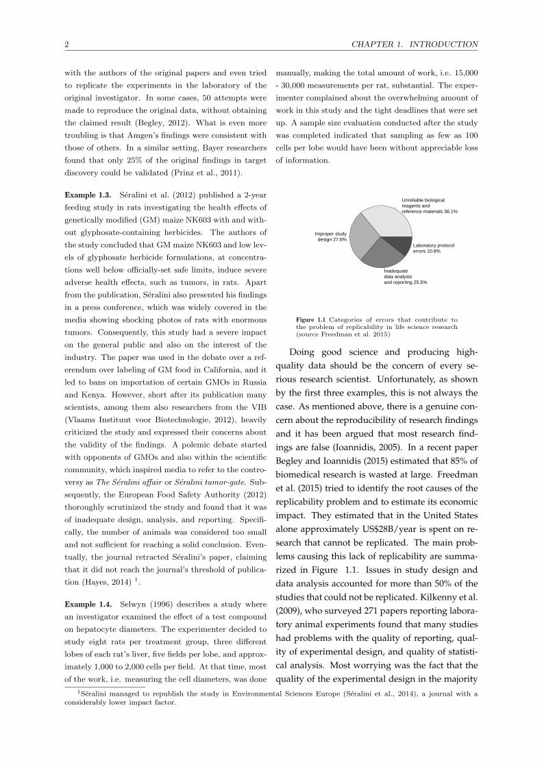
Figure 4.2 Morphometric analysis of the diameter ofbile canaliculi in wild-type and Cx32-deficient liver.Means±SEM from three livers. *: P<0.005 (afterTemme et al. (2001))
Example 4.1. Temme et al. (2001) compared two ge-
netic strains of mice, wild-type and connexin 32 (Cx32)-
deficient. They measured the diameters of bile canali-
culi in the livers of three wild-type and of three Cx32-
deficient animals, making several observations on each
liver. Their results are shown in Figure 4.2. It should
be clear that Temme et al. (2001) mistakenly took cells,
which were the observational units, for experimental
units and used them also as units of analysis. If we
consider the genotype as the treatment, then it is clear
that not the cell but the animal is the experimental unit.
Moreover, cells from the same animal will be more alike
than cells from different animals. This interdependency
of the cells invalidates the statistical analysis, as it was
carried out by the investigators. Therefore, the correct
experimental unit and unit of analysis is the animal,
not the cell. Hence, there were only three experimental
units per treatment, certainly not 280 and 162 units1.
The correct method of analysis calculates for each an-
imal the average cell diameter and takes this value as
the response variable.
Mistakes as in the above example are abundantwhenever microscopy is concerned and the indi-vidual cell is used as the experimental unit. Onecould wonder whether these are mistakes madeout of ignorance or out of convenience. The con-cern is even greater when such studies get pub-lished in peer reviewed high impact scientific jour-nals.
Independence of units can be an issue of partic-ular concern in studies when animals are housedtogether in cages. In this case, independence of theexperimental units is not always guaranteed, as isshown by the following example.
Example 4.2. Rivenson et al. (1988) studied the toxic-
ity of N-nitrosamines in rats and described their exper-
imental set-up as:
The rats were housed in groups of 3 in solid-
bottomed polycarbonate cages with hard-
wood bedding under standard conditions
diet and tap water with or without N-
nitrosamines were given ad libitum.
Since the treatment was supplied in the drinking wa-
ter, it is impossible to provide different treatments to
any two individual rats. Furthermore, the responses
obtained within the different animals within a cage can
be considered to be dependent upon one another in the
sense that the occurrence of extreme values in one unit
can affect the result of another unit. Therefore, the ex-
perimental unit here is not the single rat, but the cage.
An identical problem with the independence ofthe basic units is found in the study by Séraliniet al. (2012). In their study, rats were housed ingroups of two per cage and the treatment waspresent in the food delivered to the cages.
Even when the animals are individually treated,e.g. by injection, group-housing can cause ani-mals in the same cage to interact which would in-validate the assumption of independence of units.
1If we recalculate the standard errors of the mean (SEM) using the appropriate number of experimental units, thenthey are a factor 7-10 larger than the reported ones.

4.4. VARIATION IS OMNIPRESENT 15
For instance, in studies with rats, a socially domi-nant animal may prevent others from eating at cer-tain times. Mice housed in a group usually lie to-gether, thereby reducing their total surface area.A reduced heat loss per animal in the group isthe result. Due to this behavioral thermoregulation,their metabolic rate is altered (Ritskes-Hoitingaand Strubbe, 2007).
Nevertheless, single housing of gregarious ani-mal species is considered detrimental to their wel-fare and regulations in Europe concerning animalwelfare insist on group housing of such species(Council of Europe, 2006). However, when animalsare housed together, the cage rather than the indi-vidual animal should be considered as the exper-imental unit (Fry, 2014; Gart et al., 1986). Statisti-cal analysis should take this into account by usingappropriate techniques. Fortunately, as is pointedout by (Fry, 2014), when the cage is the experimen-tal unit, the total number of animals needed is notjust a simple multiple of the number of animalsper cage and the number of experimental units re-quired. An experiment requiring 10 animals pertreatment group when housed individually is al-most equivalent to an experiment with 12 animalsdistributed over 4 cages per treatment. This is il-lustrated in the following example.
Example 4.3. Consider the study by (Temme et al.,
2001), sample size calculations (see Chapter 6) show
that 12 animals per treatment group and 25 cells per
animal are required for each treatment group. When
animals are housed individually, the standard deviation
of the mean liver cell diameters per animal is 0.415 (sim-
ulated data). In contrast, when each cage contains three
animals, the statistical analysis is based on the mean
values of the cell diameters for each cage. The stan-
dard deviation of these mean values, calculated over a
total of five cages drops to 0.250, which corresponds to
the same statistical power (see Chapter 6) as the design
with the single animals. Hence, in this case, only three
additional animals per treatment group are required to
accommodate the animal welfare regulations.
The former example does not take into accountthat, for some outcomes, the variability is expectedto be reduced when animals are more contentwhen they are group-housed, which would en-
hance the latter experiment’s efficiency (Fry, 2014).
Two-generation reproductive studies which in-volve exposure in utero are standard proceduresin teratology. Also here, the entire litter ratherthan the individual pup constitutes the experimen-tal unit (Gart et al., 1986). This also applies to otherexperiments in reproductive biology.
Example 4.4. (Fry, 2014) A drug was tested for its ca-
pacity to reduce the effect of a mutation causing a com-
mon condition. To accomplish this, homozygous mutant
female rats were randomly assigned to drug-treated and
control groups. Then they were mated with homozy-
gous mutant males, producing homozygous mutant off-
spring. Litters were weaned and pups grouped five to
a cage and the effects on the offspring were observed.
Here, although observations on the individual offspring
were made, the experimental units are the mutant dams
that were randomly assigned to treatment. Therefore,
the observations on the offspring should be averaged to
give a single figure for each dam and these data, one for
each dam, are to be used for comparing the treatments.
A single individual can also relate to several ex-perimental units. This is illustrated by the follow-ing example.
Example 4.5. (Fry, 2014) The efficacy of two agents at
promoting regrowth of epithelium across a wound was
evaluated by making 12 small wounds in a standardized
way in a grid pattern on the back of a pig. The wounds
were far enough apart for effects on each to be indepen-
dent. One of four treatments would then be applied at
random to the wound in each square of the grid. In this
case, the experimental unit would be the wound and, as
there are 12 of them, there would be three replicates for
each treatment condition.
4.4 Variation is omnipresent
Variation is everywhere in the natural world andis often substantial in the life sciences. Despite aprecise execution of the experiment, the measure-ments obtained in identically treated objects willyield different results. For example, cells grown intest tubes will vary in their growth rates and, inanimal research, no two animals will behave thesame. In general, the more complex the systemthat we study, the more factors will interact with

16 CHAPTER 4. PRINCIPLES OF STATISTICAL DESIGN
each other and the greater will be the variationbetween the experimental units. Experiments inwhole animals will undoubtedly show more varia-tion than in vitro studies on isolated organs. Whenthe variation cannot be controlled, or its sourcecannot be measured, we will refer to it as noise, ran-dom variation or error. This uncontrollable variationmasks the effects under investigation and is thereason why replication of experimental units andstatistical methods are required to extract the nec-essary information. This is in contrast to other sci-entific areas such as physics, chemistry, and engi-neering where the studied effects are much largerthan the natural variation.
4.5 Balancing internal and exter-
nal validity
Figure 4.3 The basic dilemma: balancing between in-ternal and external validity
Internal validity refers to the fact that in a well-conceived experiment the effect of a given treat-ment is unequivocally attributed to that treatment.However, the effect of the treatment is masked bythe presence of the uncontrolled variation of theexperimental material.
An experiment with a high level of internal va-lidity should have a great chance to detect the ef-fect of the treatment. If we consider the treatmenteffect as a signal and the inherent variation of ourexperimental material as noise, then a good exper-imental design will maximize the signal-to-noise ra-tio (Figure 4.3). Increasing the signal can be accom-plished by choosing experimental material that ismore sensitive to the treatment. Identification offactors that increase the sensitivity of the experi-mental material could be carried out in prelimi-nary experiments. Reducing the noise is anotherway to increase the signal-to-noise ratio. This can
be accomplished by repeating the experiment in anumber of animals, but this is not a very efficientway of reducing the noise. An alternative way fornoise reduction is by using experimental materialthat is as much alike as possible, resulting in a lownatural variability. The use of cells harvested froma single animal is an example of noise reduction byemploying experimental material that is very sim-ilar.
External validity is related to the extent that ourconclusions can be generalized to the target popu-lation (Figure 4.3). The choice of the target popula-tion, how a sample is selected from this populationand the experimental procedures used in the studyare all determinants of its external validity. Clearly,the experimental material should mimic the targetpopulation as close as possible. In animal experi-ments specifying species and strain of the animal,the age and weight range and other characteris-tics determine the target population and make thestudy as realistic and informative as possible. Ex-ternal validity can become jeopardized when wework in a highly controlled environment with veryuniform experimental material.
Thus there is a trade-off between internal andexternal validity, as one goes up, the other comesdown. Fortunately, as we will see, there are sta-tistical strategies for designing a study such thatthe noise is reduced, while the external validity ismaintained.
4.6 Bias and variability
Bias and variability (Figure 4.4) are two importantconcepts when dealing with the design of exper-iments. A good experiment will minimize or, atbest, try to eliminate bias and will control for vari-ability. By bias, we mean a systematic deviation inobserved measurements from the true value. Oneof the most important sources of bias in a study isthe way experimental units are allocated to treat-ment groups.
Example 4.6. A researcher plans to investigate the ef-
fect of an experimental treatment relative to a control

4.6. BIAS AND VARIABILITY 17
Table 4.1 Four types of bias affecting internal validity (after van der Worp et al. (2010) and Bate and Clark (2014)).
Type of bias Definition Example
Selection bias Bias caused by a non-random allocation of an-imals in treatment groups.
Do we try to avoid the less healthy animals tothe high dosage group?
Performance bias Bias caused by differences, however subtle,in levels of husbandry care given to animalsacross treatment groups.
Are sick animals in the control group given thebenefit of the doubt and kept alive longer thananimals in the high dose group?
Detection bias Bias caused when the researcher assessing theeffect of the treatment knows which treatmentthe animal received.
When assessing animal behavior, it is humannature to want to see a positive effect in yourexperiment.
Attrition bias Bias caused by unequal occurrence and han-dling of deviations from the protocol and lossto follow-up between treatment groups.
If many animals are excluded from the high-dose group, should we take this into account?
treatment. She allocates all males to the control treat-
ment and all females to the experimental treatment. At
the end of the experiment the investigator finds a strong
difference between the two treatment groups.
It is clear that the difference between the two treat-
ment groups is a biased estimate of the true treatment
effect, since it is intertwined with the difference between
the males and the females and cannot be separated from
it. Gender is, in this case, a confounding factor and we
refer to this type of bias as confounding bias.
Figure 4.4 Bias and variability illustrated by a marks-man shot at a bull’s eye
Confounding bias can enter a study throughless obvious routes. For instance, when all ani-mals assigned to a specific treatment are kept in thesame cage. Then, the effects due to the conditionsin the cage are intertwined with the effects of thetreatments. In the case where the experiment is re-stricted to a single cage per treatment, the compar-isons between the treatments will be biased (Fry,2014). The same reasoning applies to the positionof the cages in a rack (Gart et al., 1986) and the lo-cation of the rack itself (Gore and Stanley, 2005).Putting all the cages assigned to a particular treat-ment in the same rack or on the same shelf level ofthe rack can introduce confounding bias. In fact,the importance of rack location and shelf level onfood consumption, body weight, body temperatur
(Gore and Stanley, 2005; Greenman et al., 1983),and even on the occurrence of neoplasms (Green-man et al., 1984) have been demonstrated.
As shown in Table 4.1, there are four ways inwhich confounding bias can enter a study, therebyjeopardizing its internal validity (Bate and Clark,2014; van der Worp et al., 2010). It is importantthat the researcher recognizes these four sources ofbias when planning the experiment and considersprocedures that reduce their influence on the out-come of the study. We will see that randomizationand blinding are efficient strategies that adequatelydeal with the first three sources of bias.
By variability, we mean a random fluctuationabout a central value. The terms bias and variabil-ity are also related to the concepts of accuracy andprecision of a measurement process. The absenceof bias means that our measurement is accurate,while little variability means that the measurementis precise. Good experiments are as free as possi-ble from bias and variability. Of the two, bias isthe most important. Failure to minimize the biasof an experiment leads to erroneous conclusionsand thereby jeopardizes the internal validity. Con-versely, if the outcome of the experiment showstoo much variability, this can sometimes be reme-diated by refinement of the experimental methods,increasing the sample size, or other techniques. Inthis case, the study may still reach the correct con-clusions.

18 CHAPTER 4. PRINCIPLES OF STATISTICAL DESIGN
4.7 Requirements for a good ex-
periment
Cox (1958) enunciated the following requirementsfor a good experiment:
1. treatment comparisons should as far as pos-sible be free of systematic error (bias);
2. the comparisons should also be made suffi-ciently precise (signal-to-noise);
3. the conclusions should have a wide range ofvalidity (external validity);
4. the experimental arrangement should be assimple as possible;
5. uncertainty in the conclusions should be as-sessable.
These five criteria determine the basic elements ofthe design of the study. We have discussed al-ready the importance of the first three conditions inthe preceding sections, the following section pro-vides some basic strategies that can be used to ful-fill these requirements.
Figure 4.5 Overview of strategies for minimizing thebias and maximizing the signal-to-noise ratio
4.8 Strategies for minimizing bias
and maximizing signal-to-
noise ratio
To safeguard the internal validity of his study, thescientist needs to optimize the signal-to-noise ratio(Figure 4.5). This constitutes the fundamental prin-ciple of statistical design of experiments. The sig-nal can be maximized by the proper choice of themeasuring device and experimental domain. The
noise is minimized by reducing bias and variabil-ity. Strategies for minimizing the bias are based ongood experimental practice, such as the use of con-trols, blinding, the presence of a protocol, calibra-tion, randomization, random sampling, and stan-dardization. Variability can be minimized by el-ements of experimental design, such as replica-tion, blocking, covariate measurement, and sub-sampling. In addition, random sampling can beadded to enhance the external validity. We willnow consider each of these strategies in more de-tail.
4.8.1 Strategies for minimizing bias -
good experimental practice
4.8.1.1 The use of controls
In biomedical studies, a control or reference stan-dard is a standard treatment condition againstwhich all others may be compared. The controlcan either be a negative control or a positive control.The term active control is also used for the latter. Insome studies, both negative and positive controlsare present. In this case, the purpose of the positivecontrol is mostly to provide an internal validationof the experiment1.
When negative controls are used, subjects cansometimes act as their own control (self-control),in which case the subject is first evaluated un-der standard conditions (i.e. untreated). Subse-quently, the treatment is applied and the subjectis re-evaluated. This design, also called pre-postdesign, has the property that all comparisons aremade within the same subject. In general, vari-ability within a subject is smaller than betweensubjects. Therefore, this is a more efficient designthan comparing control and treatment in two sep-arate groups. However, the use of self-control hasthe shortcoming that the effect of treatment is con-founded with the effect of time, thus introducing apotential source of bias. Furthermore, blinding,which is another method to minimize bias, is im-possible in this type of design.
1Active controls play a special role in so-called equivalence or non-inferiority studies, where the purpose is to show thata given therapy is equivalent or non-inferior to an existing standard.

4.8. STRATEGIES FOR MINIMIZING BIAS AND MAXIMIZING SIGNAL-TO-NOISE RATIO 19
Another type of negative control is where onetreated group does not receive any treatment at all,i.e. the experimental units remain untouched. Justas in the previous case of self-control, untreated con-trols cannot be blinded. Moreover, applying thetreatment (e.g. a drug) often requires extra ma-nipulation of the subjects (e.g. injection). The ef-fect of the treatment is then intertwined with thatof the manipulation, and consequently, it is poten-tially biased.
Vehicle control (laboratory experiments) or placebocontrol (clinical trials) are terms that refer to a con-trol group that receives a matching treatment con-dition without the active ingredient. Another termfor this type of control, in the context of experi-mental surgery, is sham control. In the sham controlgroup subjects or animals undergo a faked opera-tive intervention that omits the step thought to betherapeutically necessary. This type of vehicle con-trol, placebo control or sham control is the mostdesirable and truly minimizes bias. In clinical re-search, the placebo-controlled trial has become thegold standard. However, in the same context ofclinical research ethical consideration may some-times preclude its application.
4.8.1.2 Blinding
Researchers’ expectations may influence the studyoutcome at many stages. For instance, the exper-imental material may unintentionally be handleddifferently based on the treatment group, or ob-servations may be biased to confirm prior beliefs.Blinding is a very useful strategy for minimizingthis subconscious experimenter bias.
In a recent survey of studies in evolutionarybiology and the life sciences at large, Holmanet al. (2015) found that in unblinded studies themean reported effect size was inflated by 27% andthe number of statistically significant findings wassubstantially larger as compared to blinded stud-ies. The importance of blinding in combinationwith randomization in animal studies was alsohighlighted by Hirst et al. (2014). Despite its im-portance, blinding of experimenters is often ne-
glected in biomedical research. For example, ina systematic review of studies on animals in non-clinical research, van Luijk et al. (2014) found thatonly 24% reported blinded assessment of the out-come, while only 15% considered blinding of thecaretaker/investigator.
Two types of blinding must be distinguished. Insingle blinding the investigators are uninformed re-garding the treatment condition of the experimen-tal subjects. Single blinding neutralizes investigatorbias. The term double blinding in laboratory exper-iments means that both the experimenter and theobserver are uninformed about the treatment con-dition of the experimental units. In clinical trialsdouble blinding means that both investigators andsubjects are unaware of the treatment condition.
Two strategies for blinding have found theirway to the laboratory: group blinding and individ-ual blinding. Group blinding involves identicalcodes, say A, B, C, etc., for entire treatment groups.The major drawback of this approach is that, whenresults accumulate, the investigator will be ableto break the code. A much better blinding strat-egy is to assign a code (e.g. sequence number) toeach experimental unit individually and to main-tain a list that indicates which code correspondsto which particular treatment. The sequence ofthe treatments in the list should be randomized.In practice, this individual blinding procedure of-ten involves an independent person that maintainsthe list and prepares the treatment conditions (e.g.drugs).
Especially when the outcome of the experimentis subjectively evaluated, blinding must be consid-ered. However, there is one situation where blind-ing does not seem to be appropriate, namely in tox-icologic histopathology. Here, the bias that wouldbe reduced by blinding is actually a bias favoringthe diagnosis of a toxicological hazard and there-fore a conservative safety evaluation, which is ap-propriate in this context (Neef et al., 2012). In con-trast, blinded evaluation would result in a reduc-tion in the sensitivity to detect anomalies. In thiscontext, Holland and Holland (2011) suggested

20 CHAPTER 4. PRINCIPLES OF STATISTICAL DESIGN
that for toxicological work both an unblinded andblinded evaluation of histologic material should becarried out.
4.8.1.3 The presence of a technical protocol
The presence of a written technical protocol, de-scribing in full detail the specific definitions ofmeasurement and scoring methods is imperativeto minimize potential bias. The technical protocolspecifies practical actions and gives guidelines forlab technicians on how to manipulate the experi-mental units (animals, etc.), the materials involvedin the experiment, the required logistics, etc. Italso gives details on data collection and process-ing. Last but not least, the technical protocol laysdown the personal responsibilities of the techni-cal staff. The importance and contents of the otherprotocol, the study protocol, will be discussed fur-ther in Chapter 8.
4.8.1.4 Calibration
Calibration is an operation that compares the out-put of a measurement device to standards ofknown value, leading to correction of the valuesindicated by the measurement device. Calibrationneutralizes instrument bias, i.e. the bias in the in-vestigator’s measurement system.
4.8.1.5 Randomization
Randomization, together with blinding, is an im-portant tool for the elimination of confoundingbias in experiments. In an overview of system-atic reviews of animal studies, Hirst et al. (2014)found that failure to randomize is likely to result inoverestimation of treatment effects across a rangeof disease areas and outcome measures.
Formal randomization, in our context, is the pro-cess of allocating experimental units to treatmentgroups or conditions according to a well-definedstochastic law1. Randomization is a critical ele-ment in proper study design. It is an objective andscientifically accepted method for the allocation ofexperimental units to treatment groups. Formal
randomization ensures that the effect of uncon-trolled sources of variability has equal probabilityin all treatment groups. In the long run, random-ization balances treatment groups on unimportantor unobservable variables, of which we are oftenunaware. Any differences that exist in these vari-ables after randomized treatment allocation arethen to be attributed to the play of chance. In otherwords, randomization is an operation that effec-tively turns lethal bias into more manageable ran-dom error (Vandenbroeck et al., 2006). The randomallocation of experimental units to treatment con-ditions provides also an unbiased estimate of thestandard error of the treatment effects, makes ex-perimental units independent of one another andjustifies the use of significance tests. In this sense,randomization is a necessary condition for a rig-orous statistical analysis (Cox, 1958; Fisher, 1935;Lehmann, 1975). In addition, randomization is alsoof use as a device for blinding the experiment.
Example 4.7. In neurological research, animals are ran-
domly allocated to treatments. At the end of the exper-
imental procedures, the animals are sacrificed, slides are
made from certain target areas of the brain and these
slides are investigated microscopically. At each of these
stages, errors can arise leading to biased results if the
original randomization order is not maintained.
As shown in the above example, errors andbias can arise at various stages in the experiment.Therefore, to eliminate all possible bias, it is es-sential that the randomization procedure covers allimportant sources of variation connected with theexperimental units. In addition, as far as practical,experimental units receiving the same treatmentshould be dealt with separately and independentlyat all stages at which errors may arise. If this isnot the case, additional randomization proceduresshould be introduced (Cox, 1958). To summarize,randomization should apply to each stage of theexperiment (Fry, 2014):
• allocation of independent experimental unitsto treatment groups
• order of exposure to test alteration within anenvironment
1By the term stochastic is meant that it involves some elements of chance, such as picking numbers out of a hat, orpreferably, using a computer program to assign experimental units to treatment groups.

4.8. STRATEGIES FOR MINIMIZING BIAS AND MAXIMIZING SIGNAL-TO-NOISE RATIO 21
• order of measurement
Therefore, when the cage is the experimental unit,the arrangement of cages within the rack or room,the administration of substances, the taking ofsamples, etc. should all be randomized, eventhough this adds an extra burden to the labora-tory staff. Of course, this can be accomplished bymaintaining the original randomization sequencethroughout the experiment.
Formal randomization requires the use of a ran-domization device. This can be the tossing of a coin,use of randomization tables (Cox, 1958), or use ofcomputer software (Kilkenny et al., 2009). Meth-ods of randomization using MS Excel and the R sys-tem (R Core Team, 2017) are contained in AppendixC.
Some investigators are convinced that not ran-domization, but a systematic arrangement is the pre-ferred way to eliminate the influence of uncon-trolled variables. For example, when one wantsto compare two treatments A and B, one possi-bility is to set up pairs of experimental units andalways assign treatment A to the first member ofthe pair and B to the remaining unit. However,if there is a systematic effect such that the firstmember of each pair consistently yields a higheror lower result than the second member, the esti-mated treatment effect will be biased. To accom-modate for this, some researchers devised rathersmart arrangements, e.g. the alternating sequenceAB, BA, AB, BA,. . . . However, here too it cannotbe excluded that a particular pattern in the uncon-trolled variability coincides with this arrangement.For instance, if 8 experimental units are tested inone day, the first unit on a given day will alwaysreceive treatment A. Furthermore, when a system-atic arrangement has been applied, the statisticalanalysis is based on the false assumption of ran-domness and can be totally misleading.
Researchers are sometimes tempted to improveon the random allocation of animals by re-arrangingindividuals so that the mean weights are almostidentical. However, by reducing the variability
between the treatment groups, as is done in Fig-ure 4.6, the within-group variability is altered andcan now differ between groups, thereby reducingthe precision of the experiment and invalidatingthe statistical analysis. Later, we will see that therandomized block design instead of a systematicarrangement is the correct way of handling theselast two cases.
Figure 4.6 Trying to improve the random allocationby reducing the intergroup variability increases theintragroup variability
Formal randomization must be distinguished fromhaphazard allocation to treatment groups (Kilkennyet al., 2009). For example, an investigator wishesto compare the effect of two treatments (A, B) onthe body weight of rats. All twelve animals are de-livered in a single cage to the laboratory. The re-searcher then takes six animals out of the cage andassigns them to treatment A, while the remaininganimals will receive treatment B. Although, manyscientists would consider this as a random assign-ment, it is not. Indeed, one could imagine the fol-lowing scenario: heavy animals react slower andare easier to catch than the smaller animals. Conse-quently, the first six animals will on average weighmore than the remaining six.
Example 4.8. An important issue in the design of an ex-
periment is the moment of randomization. In an exper-
iment, brain cells were taken from animals and placed
in Petri dishes, such that one Petri dish corresponded
to one particular animal. The Petri dishes were then
randomly divided into two groups and placed in an in-
cubator. After 72 hrs incubation, one group of Petri
dishes was treated with the experimental drug, while
the other group received solvent.
Although the investigators made a serious effort to in-
troduce randomization in their experiment, they over-
looked the fact the placement of the Petri dishes in the
incubator introduced a systematic error. Instead of ran-
domly dividing the Petri dishes into two groups at the
start of the experiment, they should have made random
treatment allocation after the incubation period.
As pointed out before, it is important that the

22 CHAPTER 4. PRINCIPLES OF STATISTICAL DESIGN
randomization covers all substantial sources of varia-tion connected with the experimental units. As arule, randomization should be performed imme-diately before treatment application. Furthermore,after the randomization process has been carriedout the randomized sequence of the experimentalunits must be maintained; otherwise, a new ran-domization procedure is required.
4.8.1.6 Random sampling
Using a random sample in our study increases itsexternal validity and allows us to make a broad in-ference, based upon a population model of infer-ence (Lehmann, 1975). However, in practice, itis often difficult or impractical to conduct studieswith true random sampling. For instance, clini-cal trials are usually conducted using eligible pa-tients from a small number of study sites; whileanimal experiments are based on the available an-imals. This certainly limits the external validity ofthese studies and is one of the reasons that the re-sults are not always replicable.
In some cases, maximizing the external validityof the study is of great importance. This is es-pecially the case in studies that attempt to makea broad inference towards the target population(population model), like gene expression exper-iments that try to relate a specific pathology tothe differential expression of certain genes probes(Nadon and Shoemaker, 2002). For such an exper-iment, the bias in the results is minimized only if itis based on a random sample from the target pop-ulation.
4.8.1.7 Standardization
Standardization of the experimental conditions isan effective way to minimize the bias. In addition,it also can also be used to reduce the intrinsic vari-ability in the results. Examples of standardizationof the experimental conditions are the use of ge-netically or phenotypically uniform animals, envi-
ronmental and nutritional control, acclimatization,and standardization of the measurement system.As discussed before, too much standardization ofthe experimental conditions can jeopardize the ex-ternal validity of the results.
4.8.2 Strategies for controlling variability
- good experimental design
4.8.2.1 Replication
Ronald Fisher1 noted in his pioneering book TheDesign of Experiments that replication at the levelof the experimental unit serves two purposes. Thefirst is to increase the precision of estimation andthe second is to supply an estimate of error bywhich the significance of the comparisons is to bejudged.
The precision of an experiment depends on thestandard deviation2 (σ) of the experimental mate-rial and inversely on the number of experimentalunits (n). In a comparative experiment with twotreatment groups (X1) and (X2) and an equal num-ber of experimental units per treatment group, thisprecision is quantified by the standard error of thedifference between the two averages (X1 − X2) as:
σX1−X2= σ ×
√2/n (4.1)
where σ is the common standard deviation and n
is the number of experimental units in each treat-ment group.
The standard deviation is composed of the in-trinsic variability of the experimental material andthe precision of the experimental work. Reduc-tion of the standard deviation is only possible toa limited extent by refining experimental proce-dures. However, one can by increasing the num-ber of experimental units effectively enhance theexperiment’s precision. Unfortunately, due to theinverse square-root dependence of the standard er-ror on the sample size, this is not an efficient way to
1Sir Ronald Aylmer Fisher (Londen,1890 - Adelaide 1962) is considered a genius who almost single-handedly createdthe foundations of modern statistical science and experimental design.
2The standard deviation refers to the variation of the individual experimental units, whereas the standard error refersto the random variation of an estimate (mostly the mean) from a whole experiment. The standard deviation is a basicproperty of the underlying distribution and, unlike the standard error, is not altered by replication.

4.8. STRATEGIES FOR MINIMIZING BIAS AND MAXIMIZING SIGNAL-TO-NOISE RATIO 23
Figure 4.7 The effect of blocking illustrated by a study of the effect of diet on running speed of dogs. Nottaking age of the dog into account (left panel) masks most of the effect of the diet. In the right paneldogs are grouped (blocked) according to age and comparisons are made within each age group. The latterdesign is much more efficient.
control the precision. Indeed, the standard error ishalved by a fourfold increase in the number of ex-perimental units, but a hundredfold increase in thenumber of units is required to divide the standarderror by ten. In other words, replication at the level ofthe experimental unit is an effective but expensive strat-egy to control variability. As we will see later, choos-ing an appropriate experimental design that takesinto account the different sources of variability thatcan be identified, is a more efficient way to increasethe precision.
4.8.2.2 Subsampling
As mentioned above, reduction of the standard de-viation is only possible to a very limited extent.This can be accomplished by standardization ofthe experimental conditions, but also this methodis limited, and it jeopardizes the external valid-ity of the experiment. However, in some exper-iments, it is possible to manipulate the physicalsize of the experimental units. In general, units ofa larger size will show a smaller relative variabil-ity than units of a smaller size, which results in animproved precision of the estimates. In still otherexperiments, there are multiple levels of sampling.The process of taking samples below the primarylevel of the experimental unit is known as subsam-pling (Cox, 1958; Selwyn, 1996) or pseudoreplica-tion (Fry, 2014; Lazic, 2010; LeBlanc, 2004). The ex-periment reported by Temme et al. (2001) wherethe diameter of many liver cells was measured in3 animals/experimental condition, is an exampleof subsampling with animals at the primary leveland cells at the subsample level. Multiple obser-
vations or measurements made over time are alsopseudoreplications or subsamples. In biologicaland chemical analyses, it is standard practice toduplicate or triplicate independent determinationson samples from the same experimental unit. Inthis case samples and determinations within sam-ples constitute two distinct levels of subsampling.
When subsampling is present, the standard de-viation σ used in the comparison of the treat-ment means is composed of the variability be-tween the experimental units (between-unit vari-ability) and the variability within the experimentalunits (within-unit variability). It can be shown thatin the presence of subsampling, the overall stan-dard deviation of the experiment is equal to:
σ =
√σ2n +
σ2m
m(4.2)
where n and m are the number of experimen-tal units and subsamples and σn and σm the be-tween sample and within sample standard devia-tion. Equation 4.1, which defined the precision ofthe comparative 2-treatments experiment, now be-comes:
σX1−X2=
√2
n(σ2n +
σ2m
m) (4.3)
Thus, by increasing the number of experimentalunits n we reduce the total variability, while thesubsample replication m only affects the within-unit variability. A large number of subsamplesmakes only sense when the variability of the mea-surement at the sub-level σm is substantial as com-pared to the between-unit variability σn. How todetermine the required number of subsamples will

24 CHAPTER 4. PRINCIPLES OF STATISTICAL DESIGN
be discussed in Section 6.6. As a conclusion, wecan say that subsample replication is not identical andnot as effective as replication on the level of the true ex-perimental unit.
4.8.2.3 Blocking
Example 4.9. Consider a (hypothetical) study to com-
pare the effect of two diets on running speed of dogs.
We can carry out the experiment by taking six dogs
of varying age and randomly allocating three dogs to
diet A and the three remaining to diet B. However, as
shown in the left panel of Figure 4.7, the variability be-
tween dogs will mask to a great extent the effect of diet.
A more intelligent way to set up the experiment is to
group the dogs by age and make all comparisons within
the same age group, thus removing the effect of different
ages. This is illustrated in the right panel of Figure 4.7.
With the variability due to age removed, the effect of
the diets within the age groups is much more apparent.
If we can identify one or more factors otherthan the treatment condition as potentially influ-encing the outcome of the experiment, then it maybe appropriate to group the experimental units onthese factors. Such groupings are referred to asblocks or strata. Units within a block are then ran-domly assigned to the treatments. Examples ofblocking factors are plate (in microtiter plate ex-periments), animal, cage, litter, date of experiment,or based on categorizations of continuous base-line characteristics such as body weight, baselinemeasurement of the response, etc. What we effec-tively do by blocking, is to partition the variationbetween the individuals into variation betweenblocks and variation within blocks. If the block-ing factor has an important effect on the response,then the between-block variation is much greaterthan the within block variation. We will take thisinto account in the analysis of the data (analysis ofvariance or ANOVA with blocks as an additionalfactor). Comparisons of treatments are then car-ried out within blocks, where the variation is muchsmaller. Blocking is an effective and efficient wayto enhance the precision of the experiment. Fur-thermore, blocking allows reducing the bias dueto an imbalance in baseline characteristics that areknown to affect the outcome. However, block-ing does not eliminate the need for randomiza-
tion. Within each block treatments are randomlyassigned to the experimental units, thus remov-ing the effect of the remaining unknown sourcesof bias.
Figure 4.8 Results of an experiment with baseline ascovariate. There is a linear relationship between thecovariate and the response and this relationship isthe same in both treatment groups.
4.8.2.4 Covariates
Figure 4.9 Additive model with a linear covariate ad-justment
Blocking on a baseline characteristic such asbody weight is one possible strategy to elimi-nate the variability induced by the heterogeneityin weight of the animals or patients. Instead ofgrouping in blocks, or in addition to, one can alsomake use of the actual value of the measurement.Such a concomitant measurement is referred to asa covariate. It is an uncontrollable but measur-able attribute of the experimental units (or theirenvironment) that is unaffected by the treatments butmay have an influence on the measured response.Examples of covariates are body weight, age, am-bient temperature, measurement of the responsevariable before treatment, etc. The covariate filtersout the effect of a particular source of variability.Rather than blocking it represents a quantifiable at-tribute of the system studied. The statistical modelunderlying the design of an experiment with co-variate adjustment is conceptualized in Figure 4.9.The model implies that there is a linear relation-ship between the covariate and the response and

4.9. SIMPLICITY OF DESIGN 25
that this relationship is the same in all treatmentgroups. In other words, there is a series of par-allel curves, one per treatment group, relating theresponse to the covariate. This is exemplified inFigure 4.8, showing the results of an experimentwith two treatment groups in which the baselinemeasurement of the response variable served as acovariate. There is a linear relationship betweenthe covariate and the response and this is almostthe same in both treatment groups, as is shown bythe fact that the two lines are almost parallel to oneanother.
4.9 Simplicity of design
In addition to external validity, bias, and precision,Cox (1958) also stated that the design of our exper-iment should be as simple as possible. When thedesign of the experiment is too complex, it maybe difficult to ensure adherence to a complicatedschedule of alterations, especially if these are tobe carried out by relatively unskilled people. Anuncomplicated experimental design has the addi-tional advantage that the statistical analysis willalso be straightforward, without making unrea-sonable assumptions.
4.10 The calculation of uncer-
tainty
This is the last of Cox’s precepts for a good ex-periment (see Section 4.7, page 17). It is the onlystatistical requirement, but it is also the most im-portant one. Unfortunately, it is also the require-ment that researchers often neglect. Fisher (1935)already lamented that:
It is possible, and indeed it is all too fre-quent, for an experiment to be so conducted
that no valid estimate of error is available.
Without the ability to estimate the error1, there isno basis for statistical inference. Therefore, in awell-conceived experiment, we should always beable to calculate the uncertainty in the estimatesof the treatment comparisons. This usually meansestimating the standard error of the difference be-tween the treatment means. To make this calcu-lation in a rigorous manner, the set of experimen-tal units must respond independently to a specifictreatment and may only differ in a random wayfrom the set of experimental units assigned to theother treatments. This requirement again stressesthe importance of the independence of the experi-mental units and the randomness of the treatmentallocation.
Table 4.2 Multiplication factor to correct for the bias inestimates of the standard deviation based on small samples,
after Bolch (1968).
n Factor
2 1.2533 1.1284 1.0855 1.0646 1.051
When the number of experimental units issmall, the sample estimate of the standard devia-tion σ is biased and underestimates the true stan-dard deviation2. A multiplication factor to correctfor this bias for normal distributions is given in Ta-ble 4.2. For a sample size of 3, the estimate shouldbe increased with 13% to obtain the actual stan-dard deviation.
Alternatively, one can also make use of the re-sults of previous experiments to guesstimate thenew experiment’s standard deviation. However,we then make the strong assumption that randomvariation is the same in the new experiment.
1There is a big difference between the calculation of the standard error and its validity as an estimator of the truepopulation standard error, which depends on some stringent criteria
2See page 48 for more details on the uncertainty in estimates of the standard deviation

26 CHAPTER 4. PRINCIPLES OF STATISTICAL DESIGN

5. Common Designs in Biological
Experimentation
And so it was ... borne in upon me that very often, when the most elaborate statistical refinementspossible could increase the precision by only a few percent, yet a different design involving little or noadditional experimental labour might increase the precision two-fold, or five-fold or even more
R. A. Fisher (1962)
There are a multitude of designs that oneshould consider when planning an experiment,some of which are employed more commonly thanothers in the area of biological research. Unfor-tunately, the literature about experimental designis littered with technical jargon, which makes itsunderstanding quite a challenge. To name a few,there are completely randomized designs, ran-domized complete block designs, factorial designs,split plot designs, Latin square designs, Greco-Latin squares, Youden square designs, lattice de-signs, Placket-Burman designs, simplex designs,Box-Behrken designs, etc.
It helps to find our way through this jungle ofdesigns by keeping in mind that the fundamen-
tal principle of experimental design is to provide asynthetic approach to minimize bias and control vari-ability. Furthermore, as shown in Figure 5.1, wecan consider each of the specialized experimentaldesigns as integrating three different aspects of thedesign (Hinkelmann and Kempthorne, 2008):
• the treatment design,
• the error-control design,
• the sampling & observation design.
The treatment design is concerned about whichtreatments are to be included in the experimentand is closely linked to the goals and aims of thestudy. Should a negative or positive control beincorporated in the experiment, or should both
Figure 5.1 The three aspects of the design determine its complexity and the required resources
27

28 CHAPTER 5. COMMON DESIGNS IN BIOLOGICAL EXPERIMENTATION
be present? How many doses or concentrationsshould be tested and at which level? Is the inter-action of two treatment factors of interest or not?The error-control design implements the strategiesthat we learned in Section 4.8.2 to filter out dif-ferent sources of variability. The sampling & obser-vation aspect of our experiment is about how ex-perimental units are sampled from the population,how and how many subsamples should be drawn,etc.
These three aspects of experimental design de-termine the complexity of the study and the re-quired resources. The number of treatments, thenumber of blocks, and the standard error governthe required resources, i.e. the number of experi-mental units, of a study. The more treatments orthe more blocks, the more experimental units areneeded. The complexity of the experiment is deter-mined by the underlying statistical model of Fig-ure 4.1. In particular, the error-control design de-fines the study’s complexity. The randomizationprocess is a major part of this error-control design.As argued before, a justified and rigorous estima-tion of the standard error is only possible in a ran-domized experiment. Randomization has the ad-ditional advantage that it distributes the effects ofuncontrolled variability randomly over the treat-ment groups.
Replication of experimental units is a key fac-tor for an effective experiment. The number ofexperimental units should be sufficient, such thatan adequate number of degrees of freedom areavailable for estimating the experiment’s precision(standard error). This parameter is related to thesampling & observation aspect of the design.
These three aspects of experimental design pro-vide a framework for classifying and comparingthe different types of experimental design that areused in the life sciences. As we will see, eachof these designs has its advantages and disadvan-tages.
5.1 Error-control designs
5.1.1 The completely randomized design
The completely randomized design is the mostcommon and simplest possible error-control de-sign for comparative experiments. Each experi-mental unit is randomly assigned to exactly onetreatment condition. This is often the default de-sign used by investigators who do not really thinkabout design problems.
In the following example of a completely ran-domized design, the investigators used random-ization, blinding, and individual housing of ani-mals to guarantee the absence of systematic errorand independence of experimental units.
Example 5.1. An experiment was set up to assess the
effect of chronic treatment with two experimental drugs
as compared to their vehicles on the proliferation of gas-
tric epithelial cells in rats. A total of 40 rats were ran-
domly divided into four groups of each ten animals, us-
ing the MS Excel randomization procedure described
in Appendix C. To guarantee the independence of the
experimental units, the animals were kept in separate
cages1. Cages were distributed over the racks according
to their sequence number. Blinding was accomplished
by letting the sequence number of each animal corre-
spond to a given treatment. One laboratory worker was
familiar with the codes and prepared the daily drug so-
lutions. Treatment codes were concealed from the rest
of the laboratory staff that was responsible for the daily
treatment administration and final histological evalua-
tion.
The advantage of the completely randomizeddesign is that it is simple to implement, as experi-mental units are simply randomized to the varioustreatments. The obvious disadvantage is the lackof precision in the comparisons among the treat-ments, which is based on the variation between theexperimental units.
1The experiment dates from before the implementation of the guidelines regarding group housing of gregarious animals(Council of Europe, 2006). However, the design is easily adapted to designs with animals housed in groups of three or four.The total number of animals should then be raised to 48 or 60 and cages are the experimental units.

5.1. ERROR-CONTROL DESIGNS 29
Figure 5.2 Outline of a paired experiment on isolated cardiomyocytes. Cardiomyocytes of a single animalwere isolated and seeded in plastic Petri dishes. From the resulting five pairs of Petri dishes, one memberwas randomly assigned to drug treatment, while the remaining member received the vehicle.
5.1.2 The randomized complete block de-
sign
The concept of blocking as a tool to increase effi-ciency by enhancing the signal-to-noise ratio hasalready been introduced in Section 4.8.2.3 (page24). The basic idea behind blocking is to parti-tion the total set of experimental units into sub-sets (blocks) that are as homogeneous as possible.(Hinkelmann and Kempthorne, 2008). In a ran-domized complete block design, a single isolatedextraneous source of variability (block) closely re-lated to the response is eliminated from the com-parisons between treatment groups. The designis complete since all treatments are applied withineach block. Consequently, treatments can be com-pared with one another within the blocks. Therandomization procedure now randomizes treat-ments separately within each block. The random-ized complete block design is a very useful and re-liable error-control design since all treatment com-parisons are made within a block. When a studyis designed such that the number of experimentalunits within each block and treatment is equal, itis called a balanced design. A few examples willillustrate its use in the laboratory.
Example 5.2. In the completely randomized design
of Example 5.1 (page 28), the rats were individually
housed in a rack consisting of five shelves of each eight
cages. On different shelves, rats are likely to be ex-
posed to multiple varieties of light intensity, tempera-
ture, humidity, sounds, views, etc. As argued in Section
4.6, housing conditions can lead to biased outcomes and
also here, the investigators suspected shelf level to af-
fect the results. Therefore, they decided to switch to a
randomized complete block design in which the blocks
corresponded to the five shelves of the rack. Within
each block separately the animals were randomly allo-
cated to the treatments, such that in each block each
treatment condition occurred exactly twice. This ex-
ample also illustrates that, although all treatments are
present in each block in a randomized complete block
design, more than one experimental unit per block can
be allocated to a treatment condition.
There are two main reasons for choosing a ran-domized complete block design above a com-pletely randomized design. Suppose there is anextraneous factor that is strongly related to the out-come of the experiment. It would be most unfor-tunate if our randomization procedure yielded adesign in which there was a great imbalance onthis factor. If this were the case, the comparisonsbetween treatment groups would be confoundedwith differences in this nuisance factor and be bi-ased. The second main reason for a randomizedcomplete block design is its possibility to consid-erably reduce the error variation in our experi-ment, thereby making the comparisons more pre-cise. The main objection to a randomized completeblock design is that it makes the strong assumptionthat there is no interaction between the treatment vari-able and the blocking characteristics, i.e. that the effectof the treatments is the same among all blocks.
Sometimes we want to include two or moreblocking factors to reduce the unexplained varia-tion in our experiment. In this case, we can treatthe combinations of the blocking factor as a sin-gle new blocking factor and use it in a randomizedcomplete block design.
Example 5.3. In addition to the shelf height, the in-
vestigators also suspected that the body weight of the
animals might affect the results. Therefore, the animals
were numbered in order of increasing body weight. The
first eight animals were placed on the top shelf and ran-
domized to the four treatment conditions, then the next
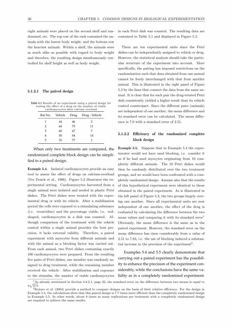
30 CHAPTER 5. COMMON DESIGNS IN BIOLOGICAL EXPERIMENTATION
eight animals were placed on the second shelf and ran-
domized, etc. The top row of the rack contained the an-
imals with the lowest body weight, and the bottom row
the heaviest animals. Within a shelf, the animals were
as much alike as possible with regard to body weight
and therefore, the resulting design simultaneously con-
trolled for shelf height as well as body weight.
5.1.2.1 The paired design
Table 5.1 Results of an experiment using a paired design fortesting the effect of a drug on the number of viable
cardiomyocytes after calcium overload
Rat No. Vehicle Drug Drug - Vehicle
1 44 46 22 64 75 113 60 67 74 50 64 145 76 77 1
When only two treatments are compared, therandomized complete block design can be simpli-fied to a paired design.
Example 5.4. Isolated cardiomyocytes provide an easy
tool to assess the effect of drugs on calcium-overload
(Ver Donck et al., 1986). Figure 5.2 illustrates the ex-
perimental setting. Cardiomyocytes harvested from a
single animal were isolated and seeded in plastic Petri
dishes. The Petri dishes were treated with the exper-
imental drug or with its vehicle. After a stabilization
period the cells were exposed to a stimulating substance
(i.e. veratridine) and the percentage viable, i.e. rod-
shaped, cardiomyocytes in a dish was counted. Al-
though comparison of the treatment with the vehicle
control within a single animal provides the best pre-
cision, it lacks external validity. Therefore, a paired
experiment with myocytes from different animals and
with the animal as a blocking factor was carried out.
From each animal, two Petri dishes containing exactly
100 cardiomyocytes were prepared. From the resulting
five pairs of Petri dishes, one member was randomly as-
signed to drug treatment, while the remaining member
received the vehicle. After stabilization and exposure
to the stimulus, the number of viable cardiomyocytes
in each Petri dish was counted. The resulting data are
contained in Table 5.1 and displayed in Figure 5.3.
There are ten experimental units since the Petri
dishes can be independently assigned to vehicle or drug.
However, the statistical analysis should take the partic-
ular structure of the experiment into account. More
specifically, the pairing has imposed restrictions on the
randomization such that data obtained from one animal
cannot be freely interchanged with that from another
animal. This is illustrated in the right panel of Figure
5.3 by the lines that connect the data from the same an-
imal. It is clear that for each pair the drug-treated Petri
dish consistently yielded a higher result than its vehicle
control counterpart. Since the different pairs (animals)
are independent of one another, the mean difference and
its standard error can be calculated. The mean differ-
ence is 7.0 with a standard error of 2.51.
5.1.2.2 Efficiency of the randomized complete
block design
Example 5.5. Suppose that in Example 5.4 the exper-
imenter would not have used blocking, i.e. consider it
as if he had used myocytes originating from 10 com-
pletely different animals. The 10 Petri dishes would
then be randomly distributed over the two treatment
groups, and we would have been confronted with a com-
pletely randomized design. Assume also that the results
of this hypothetical experiment were identical to those
obtained in the paired experiment. As is illustrated in
the left panel of Figure 5.3, the two groups largely over-
lap one another. Since all experimental units are now
independent of one another, the effect of the drug is
evaluated by calculating the difference between the two
mean values and comparing it with its standard error1
Obviously, the mean difference is the same as in the
paired experiment. However, the standard error on the
mean difference has risen considerably from a value of
2.51 to 7.83, i.e. the use of blocking induced a substan-
tial increase in the precision of the experiment2.
Examples 5.4 and 5.5 clearly demonstrate thatcarrying out a paired experiment has the possibil-ity to enhance the precision of the experiment con-siderably, while the conclusions have the same va-lidity as in a completely randomized experiment.
1As already mentioned in Section 4.8.2.1, page 22, the standard error on the difference between two means is equal toσ√
2/n2Kutner et al. (2004) provide a method to compare designs on the basis of their relative efficiency. For the design in
Example 5.4, the calculations show that this paired design is 7.7 times more efficient than the completely randomized designin Example 5.5. In other words, about 8 times as many replications per treatment with a completely randomized designare required to achieve the same results.

5.1. ERROR-CONTROL DESIGNS 31
Treatment
% V
iabl
e M
yocy
tes
50
60
70
Vehicle Drug
Treatment
% V
iabl
e M
yocy
tes
50
60
70
Vehicle Drug
Figure 5.3 Gain in efficiency induced by blocking illustrated in a paired design. In the left panel, themyocyte experiment is considered as a completely randomized design in which the two samples largelyoverlap one another. In the right panel the lines connect the data of the same animal and show a markedeffect of the treatment.
However, the forming of blocks of experimentalunits is only successful when the criterion uponwhich the pairing is based, is related to the out-come of the experiment. Using as a blocking fac-tor, a characteristic that does not have a substantialeffect on the response variables is worse than use-less since the statistical analysis will lose power bytaking the blocking into account. This can be ofparticular importance for small sized experiments.The following example illustrates such a case.
Treatment
neur
ons/
mm
0
50
100
Vehicle Drug
Figure 5.4 A case where the blocking criterium (ani-mal pair) is not related to the response.
Example 5.6. In this study (Haseldonckx et al., 1997),
the neuronal protective effect of a drug was assessed in
a rat model of brain ischemia. Global cerebral ischemia
was induced in rats by bilateral clamping of the carotid
arteries and severe hypotension during 9 minutes. Five
minutes after termination of ischemia, treatment with
an experimental drug or its vehicle was started. Seven
days after the insult, the animals were sacrificed and
the number of viable neurons/mm in the CA1 layer of
the hippocampus was evaluated in a blinded manner.
The investigators hypothesized that there would be a
substantial variability connected to the particular day
of the week an animal arrived in the study. Therefore,
to eliminate this source of variability and possible bias,
animals entered the study in pairs. From each pair,
one animal was randomly selected and treated with the
drug, while the remaining animal received the drug’s
vehicle. The results of an experiment on 26 animals
(13 pairs) are shown in Figure 5.4. Apparently, forming
pairs on the basis of the assumption of substantial daily
variability was not very successful. There were animals
treated with vehicle for which the outcome was low,
while their drug treated counterparts showed a large
number of neurons and vice versa. Actually, the lin-
ear correlation between the outcome of the vehicle and
drug treated animals is as low as -0.05. The mean dif-
ference between the controls and treated animals is 51.2
neurons/mm, with a standard error of 12.3. Next, let
us consider the experiment as a completely randomized
design, i.e. without any restrictions on the randomiza-
tion, then the standard error on the difference between
the two means is 12.0, which is almost the same. How-
ever, the standard error of the completely randomized
experiment has 24 degrees of freedom, while that for
the paired experiment is based on only 12 degrees of
freedom. Consequently, in this case, the paired experi-
ment was less efficient than the completely randomized
design, since the forming of pairs led to a serious loss in

32 CHAPTER 5. COMMON DESIGNS IN BIOLOGICAL EXPERIMENTATION
the degrees of freedom involved in the calculation of the
standard error. This example demonstrates that block-
ing is only effective when the within-block variation is
much less than the between-block variation.
5.1.3 Incomplete block designs
In some circumstances, the block size is smallerthan the number of treatments, and consequently,it is impossible to assign all treatments within eachof the blocks. When a particular comparison is ofspecific interest, such as comparison with control,it is wise to include it in each of the blocks.
Table 5.2 Balanced incomplete block design for Example 5.7with treatments A,B,C and D
Sibling lamb pair
Lamb 1 2 3 4 5 6
First A A A B B CSecond B C D C D D
Balanced incomplete block designs allow allpairwise comparisons of treatments with equalprecision, using a block size that is less than thenumber of treatments. To achieve this, the bal-anced incomplete block design has to satisfy thefollowing conditions (Bate and Clark, 2014; Cox,1958):
• each block contains the same number ofunits;
• each treatment occurs the same number oftimes in the design;
• every pair of treatments occurs together inthe same number of blocks.
Balanced incomplete block designs (BIB) exist foronly certain combinations of the number of treat-ments and number and size of blocks. When look-ing for a suitable balanced incomplete block de-sign, it can happen that if we add one or moreadditional treatments, a more appropriate designis found. Alternatively, omitting one or moretreatments can yield a more efficient design (Cox,1958). Software to construct incomplete block de-signs is provided by the agricolae package in R (deMendiburu, 2016).
Example 5.7. (Anderson and McLean, 1974; Bate and
Clark, 2014). An experiment was carried out to assess
the effect that vitamin A and a protein dietary supple-
ment have on the weight gain of lambs over a 2-month
period. There were four treatments, labeled A, B, C,
and D in the study corresponding to a low dose and
a high dose of vitamin A, combined with a low dose
and a high dose of protein. A total of three replicates
per treatment was considered as sufficient, and blocking
was carried using pairs of sibling lambs, so six pairs of
siblings were used. With the number of treatments re-
stricted to two per block, the balanced incomplete block
design shown in Table 5.2 was used.
A possible layout of the experiment is obtained in Rusing the agricolae-package (de Mendiburu, 2016):
> library(agricolae)
> # Label 4 treatments A, B, C, D
> trt<-LETTERS[1:4]
> # Blocksize = 2
> # Change seed for other randomization
> design.bib(trt,2,seed=543)$sketch
Parameters BIB
==============
Lambda : 1
treatmeans : 4
Block size : 2
Blocks : 6
Replication: 3
Efficiency factor 0.6666667
<<< Book >>>
[,1] [,2]
[1,] "D" "A"
[2,] "B" "D"
[3,] "A" "B"
[4,] "C" "B"
[5,] "A" "C"
[6,] "C" "D"
It is clear that the BIB-design generated in the R-session
is equivalent to the design shown in Table 5.2.
Example 5.8. Biggers et al. (1981) use a BIB-design
to compare the effects of intrauterine injection of six
prostaglandin antagonists on the fertility of mice. Since
the lumen of each uterine horn in a mouse is not con-
nected with the other, each female can be used to com-
pare the effect of two treatments. There are six treat-
ments (antagonists) and two experimental units (uter-
ine horns) per animal. To compare the antagonists with
each other requires at least(
62
)=15 animals. Each of
the treatments is then replicated five times in the de-
sign. The BIB-design with the animal as the blocking
factor is generated in R as:

5.1. ERROR-CONTROL DESIGNS 33
> # Label 6 treatments A, B, C, D, E, F
> trt<-LETTERS[1:6]
> # Blocksize = 2
> # Change seed for other randomization
> design.bib(trt,2,seed=4338)$sketch
Parameters BIB
==============
Lambda : 1
treatmeans : 6
Block size : 2
Blocks : 15
Replication: 5
Efficiency factor 0.6
<<< Book >>>
[,1] [,2]
[1,] "D" "B"
[2,] "B" "C"
[3,] "E" "B"
[4,] "A" "F"
[5,] "D" "E"
[6,] "C" "E"
[7,] "C" "F"
[8,] "C" "D"
[9,] "A" "C"
[10,] "A" "D"
[11,] "D" "F"
[12,] "F" "B"
[13,] "E" "F"
[14,] "B" "A"
[15,] "E" "A"
As noted by Biggers et al. (1981), the major draw-
back of this design is that it assumes that the effect of
a treatment in a uterine horn is local with no effects on
the contralateral horn.
The designs presented in Example 5.7 and 5.8consider only a single run of the BIB-design. How-ever, in most cases, more replicates than givenby the basic design are required. See Dean andVoss (1999) for more details on how to calculatethe required number of replicates. BIB-designswith more replicates can be generated by supply-ing an extra argument to the design.bib-function,specifying the number of replicates of the treat-ments. However, it is not always possible to obtaina balanced design, as is reported by the design.bib-function:
> # Label 6 treatments A, B, C, D, E, F
> trt<-LETTERS[1:6]
> # Block size 2,
> # 6 replicates of each treatment
> out<-design.bib(trt,2,6,seed=4338)$sketch
Change r by 5, 10, 15, 20 ...
> # replicates must be multiple of 5, so 10 is OK
> out<-design.bib(trt,2,10,seed=4338)$sketch
Parameters BIB
==============
Lambda : 2
treatmeans : 6
Block size : 2
Blocks : 30
Replication: 10
Efficiency factor 0.6
<<< Book >>>
5.1.4 Latin square designs
When the experimental units exhibit heterogene-ity in two directions, such as the rows and thecolumns of cage racks, then we require a blockdesign that accounts for both sources of variabil-ity. The Latin square design is an extension of therandomized complete block design, with blockingdone simultaneously on two characteristics that af-fect the response variable. In a Latin square design,the k treatments are arranged in a k×k square suchas in Table 5.3. Each of the four treatments A, B, C,and D occurs exactly once in each row and exactlyonce in each column. The latin square design iscategorized as a two-way block error-control design.
Table 5.3 Arrangement for a 4× 4 Latin square designcontrolling for column and row effects.
Column
Row 1 2 3 4
1 A B C D2 D A B C3 C D A B4 B C D A
Example 5.9. Gore and Stanley (2005) considered a
weight gain study in female CD-1 mice, which inves-
tigated the effect of a control vehicle and a test com-
pound administered at four different doses. The mice
were housed singly in cages across three racks using an
independent Latin square design in each rack, thereby
ensuring that all five treatment groups were present in
each row and column of every rack. The racks consisted
of five shelves (rows) of each six cages. The last column
of the rack was left empty. Table 5.4 illustrates a pos-
sible layout of the experiment. Using this design they
were able to show that the rack the animals were housed
in influenced their water intake and that the body tem-
perature of the mice depended on the row (shelf of the

34 CHAPTER 5. COMMON DESIGNS IN BIOLOGICAL EXPERIMENTATION
rack) that the cages were placed in. The authors advo-
cate the use of Latin square designs to allocate treat-
ments to cages for future trials. Specifically they warn
against the use of more practically appealing designs
such as:
putting all replicates of treatments in the same
row of cages in each of the racks;
placing all replicates of a particular treatment in
the same rack, perhaps in adjacent cages.
In either case, there is the risk of making false conclu-
sions, due to this bias.
In the above example, 5× 5 Latin squares wereused to control for the location of the cages inthe racks. Another application of Latin squares isabout experiments on neuronal protection, wherea pair of animals was tested each day, and theinvestigator expected a systematic difference notonly between the pairs but also between the animaltested in the morning and the one tested in the af-ternoon. In the biomedical laboratory, Latin squaredesigns are also used for the elimination of loca-tion effects in microwell plates (Aoki et al., 2014;Burrows et al., 1984).
Table 5.4 Arrangement for the 5× 5 Latin square design ofExample 5.9 of placing animals in cage racks. The numbers
indicate the five dose levels of the test compound (0 = vehiclecontrol, - = empty)
Column
Row 1 2 3 4 5 6
1 3 1 10 0 30 -2 1 0 3 30 10 -3 10 3 30 1 0 -4 0 30 1 10 3 -5 30 10 0 3 1 -
The main advantage of the Latin square designis that it simultaneous balances out two sources oferror. The disadvantage is the strong assumptionthat there are no interactions between the blockingvariables or between the treatment variable andblocking variables. Latin square designs are alsolimited by the fact that the number of treatments,number of rows, and number of columns mustall be equal. Fortunately, there are other arrange-ments that do not have this limitation (see (Cox,1958; Hinkelmann and Kempthorne, 2008)).
In a k×k Latin square, only k experimental unitsare assigned to each treatment group. However, itmay happen that more experimental units are re-quired to obtain an adequate precision. The Latinsquare can then be replicated and several squarescan be used to obtain the necessary sample size. Indoing this, there are two possibilities to consider.Either one stacks the squares on top of each other(or next to each other) and keeps them as separateindependent squares, or one completely random-izes the order of the rows (or columns) of the de-sign. For small experiments, such as in 2× 2 Latinsquares, keeping the squares separate is not a goodidea and leads to less precise estimation and loss ofdegrees of freedom1. However, when there is a rea-son to believe that the column (or row) effects aredifferent between the squares, it does make senseto keep the squares separate.
The R-package agricolae (de Mendiburu, 2016)can generate random Latin squares, e.g. a possiblelayout of the experiment in Example 5.9 is obtainedby:
> library(agricolae) # load package agricolae
> trt<-c("0","1","3","10","30")
> # Latin square design
> # use seed for different randomization
> design.lsd(trt, seed=3489)$sketch
[,1] [,2] [,3] [,4] [,5]
[1,] "1" "30" "10" "3" "0"
[2,] "0" "10" "3" "1" "30"
[3,] "10" "1" "0" "30" "3"
[4,] "3" "0" "30" "10" "1"
[5,] "30" "3" "1" "0" "10"
5.1.5 Incomplete Latin square designs
In Section 5.1.3, we considered balanced incompleteblock designs as randomized complete block designswhen the number of treatments is larger than theblock size. In Latin square designs the experimen-tal units are classified in two directions analogousto the rows and columns of a Latin square. Whenthe number of available units in one direction, or inboth directions, is smaller than the number of treat-ments, then we need an incomplete Latin squaredesign. We will restrict our discussion to the case
1The error degrees of freedom in a Latin square design with t treatments tested on t2 experimental units are (t−1)(t−2).When a Latin square is replicated r times, the error degrees of freedom are (t − 1)(rt − t − 1) when the squares are keptseparate and (rt − 2)(t − 1) when rows or columns of the squares are intermixed. The latter always results in a largernumber, making it more precise.

5.2. TREATMENT DESIGNS 35
where only one direction has an incomplete char-acter.
Youden Squares Youden squares are actuallyrectangles with r = t rows (t = number of treat-ments) and c < t columns. The designs com-bine the property of the Latin square design ofeliminating heterogeneity in two directions withthe property of the balanced incomplete block de-sign of comparing treatments with the same preci-sion. The designs are called Youden squares afterYouden (1937) who first introduced them. Youdensquares have the property that every treatment oc-curs in every column, but not in every row.
Example 5.10. Colquhoun (1963) describes the use of
Youden squares in an assay of gastrin in rats. Two
doses of the standard preparation of gastrin and two
doses of the preparation of unknown potency are tested
in rats. Ideally, the four preparations would be tested
in the same animal using a 4 × 4 Latin square design.
However, it was found impractable to obtain responses
from the animals to more than three treatment appli-
cations. Consequently, the fourth dose had to be given
to another animal. The authors therefore resorted to
a Youden square design where each row represents an
animal, and the columns correspond to the order of ad-
ministration.
Again, the R-package agricolae (de Mendiburu, 2016)is used to generate a Youden square design:
> library(agricolae) # load package
> trts<-c("A","B","C","D") # 4 doses of 2 drugs
> admins<-3 # administrations per animal
> outdesign <-design.youden(trts,admins,seed=3273)
> outdesign$sketch
[,1] [,2] [,3]
[1,] "A" "B" "C"
[2,] "D" "C" "B"
[3,] "B" "D" "A"
[4,] "C" "A" "D"
Randomization is obtained by changing the number in
seed. Each treatment occurs exactly once in each col-
umn and since the columns represent the order of ad-
ministration, the means of the columns can be used
to judge whether there is a difference between the re-
sponses of the first, second, or third administration.
2
5.2 Treatment designs
5.2.1 One-way layout
The examples that we discussed up to now (apartfrom Example 5.7), all considered the treatment as-pect of the design as consisting of a single factor.This factor can represent presence or absence of asingle condition or several different related treat-ment conditions (e.g. Drug A, Drug B, Drug C ).The treatment aspect of these designs is referred toas single factor or one-way layout.
5.2.2 Factorial designs
In some types of experimental work, such as in Ex-ample 5.7 (page 32), it can be of interest to assessthe joint effect of two or more factors, e.g. a highand a low dose of Vitamin A combined with a highand a low dose of protein. In Example 5.7, only twofactors were considered, each at two levels (high,low). This is a typical case of a 2 × 2 full factorialdesign, the simplest and most frequently used fac-torial treatment design. In a full factorial design,the factors and all combinations (hence full) of thelevels of the factors are studied. The design allowsestimating the main effects of the individual treat-ments, as well as their interaction effect, i.e. the de-viation from additivity of their joint effect. We willuse the 2×2 full factorial design to explore the basicconcepts of factorial designs and statistical interac-tion.
Example 5.11. (Bate and Clark, 2014) A study was
conducted to assess whether the serum chemokines JE
and KC could be used as markers of atherosclerosis de-
velopment in mice (Parkin et al., 2004). Two strains of
apolipoprotein-E-deficient (apoE-/-) mice, C3H apoE-/-
and C57BL apoE-/- were used in the study. These
mice were fed either a normal diet or a diet contain-
ing cholesterol (the Western diet). After 12 weeks the
animals were sacrificed and their atherosclerotic lesion
areas were determined. The study design consisted of
two categorical factors: Strain and Diet. The factor
Strain contained two levels: C3H apoE-/- and C57BL
apoE-/-, as did the factor Diet : normal rodent diet and
Western diet. In total there were four combinations of
factor levels:
1. C3H apoE-/- + normal diet
2. C3H apoE-/- + Western diet

36 CHAPTER 5. COMMON DESIGNS IN BIOLOGICAL EXPERIMENTATION
3. C57BL apoE-/- + normal diet
4. C57BL apoE-/- + Western diet
1500
2000
2500
3000
3500
4000
4500
5000
Diet
Lesi
on a
rea
(µ m
−2)
Normal Western
C3HC57BL
Figure 5.5 Plot of mean lesion area for the case wherethere is no interaction between Strain and Diet.
Let us consider some possible outcomes of thisexperiment.
No interaction When there is no interaction be-tween Strain and Diet, the difference between thetwo diets is the same, irrespective of the mousestrain. The lines connecting the mean values of thetwo diets are parallel to one another, as is shownin Figure 5.5. There is an overall effect of Diet, ani-mals fed with the Western diet show larger lesions,and this effect is the same in both strains. Thereis also an overall effect of the Strain. Lesions arelarger in the C3H apoE-/- than in the C57BL apoE-/-
strain and this difference is the same for both diets.
Since the difference between the diets is thesame, regardless which strain of mice they are fedto, it is appropriate to average the results fromeach diet across both strains and make a singlecomparison between the diets rather than makingthe comparison separately for each strain. In do-ing this, the external validity of the conclusions isbroadened since they apply to both strains. Be-sides, the comparison between the two strains canbe made, irrespective of the diet the animals arereceiving. C3H apoE-/- have larger lesions thanC57BL apoE-/- regardless of the diet. Both compar-isons, use all the experimental units, which makes
a factorial design a highly efficient design since allthe animals are used to test simultaneously two hy-potheses.
Moderate interaction When there is a moderate in-teraction, the direction of the effect of the first fac-tor is the same regardless of the level of the sec-ond factor. However, the size of the effect varieswith the level of the second factor. This is exem-plified by Figure 5.6, where the lines are not paral-lel, though both indicate an increase in lesion sizefor the Western diet as compared to the normaldiet. This increase is more pronounced in the C3HapoE-/- strain than in the C57BL apoE-/- animals.Hence, the C3H apoE-/- strain is more sensitive tochanges in diet.
1500
2000
2500
3000
3500
4000
4500
5000
Diet
Lesi
on a
rea
(µ m
−2)
Normal Western
C3HC57BL
Figure 5.6 Plot of mean lesion area for the case wherethere is a moderate interaction between Strain andDiet.
Strong interaction The effect of the first factor canalso be entirely dependent on the level of the sec-ond factor. This is illustrated in Figure 5.7, wherefeeding the Western diet to the C3H apoE-/- haslittle effect on lesion size, whereas the effect onC57BL apoE-/- mice is substantial. This is an exam-ple of strong interaction. The Western diet alwaysresults in bigger lesions, but the effect in the C57BLapoE-/- strain is much more pronounced than inthe C3H apoE-/- mice. Furthermore, when fed withnormal diet the C3H apoE-/- mice show a larger le-sion area than the C57BL apoE-/- strain. However,

5.2. TREATMENT DESIGNS 37
when the animals receive Western diet the oppo-site is true.
1500
2000
2500
3000
3500
4000
4500
5000
Diet
Lesi
on a
rea
(µ m
−2)
Normal Western
C3HC57BL
Figure 5.7 Plot of mean lesion area for the case wherethere is a moderate interaction between Strain andDiet.
The factorial treatment design can be combinedwith the error control designs that we encounteredin Section 5.1. For instance, Example 5.7 (page 32)illustrates a 2 × 2 factorial combined with a bal-anced incomplete block design.
It happens that researchers have planned a fac-torial experiment, but in the design and analysisphase failed to recognize it as such. In this case,they do not take full advantage of the factorialstructure for interpreting treatment effects and of-ten analyze and interpret the experiment with anincorrect procedure (Nieuwenhuis et al., 2011). Wewill come back to that in Section 9.2.1.2.
When the two factors consist of concentrationsor dosages of drugs, researchers tend to confusethe statistical concept of interaction with the phar-macological concept of synergism. However, therequirements for two drugs to be synergistic witheach other are much more stringent than just thesuperadditivity associated with the statistical con-cept of interaction (Greco et al., 1995; Tallarida,2001). It is easy to demonstrate that, due to thenonlinearity of the log-dose response relationship,superadditive effects will always be present for the
combination, since the total drug dosage has in-creased, thus implying that a drug could be syn-ergistic with itself. In connection with the 96-well plates and the presence of plate location ef-fects Straetemans et al. (2005) provide a statisticalmethod for assessing synergism or antagonism.
Higher dimensional factorial designs Up to nowwe limited our discussion to 2×2 factorial designs.An obvious way to expand these designs is by con-sidering more factors and more factor levels. For asmall number of factors (up to 4) at two levels fullfactorial designs can be used. However, for a largernumber of factors or more factor levels, the num-ber of possible combinations can become large. Forinstance, an experiment with five factors at twolevels has to deal with 32 combinations. Also, thethree-factor and higher interactions become dif-ficult to interpret (Clewer and Scarisbrick, 2001).One way of restricting the number of resources isby implementing a full factorial design with only asingle replicate. However, these unreplicated facto-rial designs (UFD) do not leave degrees of freedomfor estimation of the error component and, conse-quently, their statistical analysis requires specificprocedures (Hinkelmann and Kempthorne, 2008;Montgomery, 2013). UFD have only limited usewhen the number of factors becomes larger thansix. For instance, when eight factors are thought tobe of importance, a UFD would require 256 exper-imental units and 1024 experimental units for tenfactors.
An alternative to the UFD are the fractionated fac-torial designs (FFD). These designs ignore the pres-ence of higher-order effects at the design stage, byomitting certain treatments from the design, suchthat most of the degrees of freedom are devoted tothe main effects and low-order interactions. FFDare particularly useful when the number of factorsis large.
UFD and FFD find application in exploratorystudies that attempt to identify the possiblesources of variation in an experiment. Therefore,significance tests are not applicable for these trials.Usually, these experiments are followed by more

38 CHAPTER 5. COMMON DESIGNS IN BIOLOGICAL EXPERIMENTATION
Drug
No.
of t
umor
s
5
10
15
20
DAS Vehicle
A/J3MC
DAS Vehicle
NIH3MC
A/JUrethane
5
10
15
20
NIHUrethane
Drug
No.
of t
umor
s
5
10
15
DAS Vehicle
A/J3MC
DAS Vehicle
NIH3MC
A/JUrethane
5
10
15
NIHUrethane
Figure 5.8 Plot of simulated data for the combinations of Strain, Carcinogen, and Treatment for thecomplete dataset with 64 mice and for a reduced dataset of only the first 32 mice.
elaborate, well-designed studies in which the ear-lier findings are verified. In the following, we willsee the application of full factorial, unreplicated fullfactorial, and fractional factorial designs in the opti-mization of animal experiments.
Optimizing animal experiments by factorial designs
Optimization of animal experiments, such that themaximum signal/noise ratio is obtained, leads toexperiments in which the required number of an-imals is minimized. For this reason, investigatorscarry out experiments in which a vehicle controland a known positive control treatment are com-pared in connection with factors the investigatorcan control and that he thinks can be importantin influencing the result. The researcher will thentry to determine under which combination of fac-tors the treatment effect, i.e. the mean difference be-tween the positive control and the vehicle is max-imized. The factors that are studied are animal-related characteristics such as sex, strain, age, diet,and health status, as well as aspects of the environ-ment such as cage and group size, bedding mate-rial, etc. Other factors can be protocol-specific suchas dose level, timing and route of administration,timing of observations etc. The conventional ap-proach for finding these optimum conditions wasto vary each factor of interest one at a time, keeping
all other factors, which may influence the outcome,at a fixed level. However, as compared to factorialdesigns, this approach has certain disadvantages(Shaw et al., 2002):
• each group of animals will contribute to un-derstanding the effect of only a single factor,while in a factorial design each animal con-tributes to the understanding the effect of allthe factors under exploration;
• the conventional approach overlooks the factthat the effect of one factor can depend on thelevel of another factor (i.e. interaction);
• in a factorial design all potential factors areconsidered at the study outset, which avoidsincremental changes to multiple studies overtime.
Example 5.12. Shaw et al. (2002) describe the develop-
ment of an animal model for lung cancer. Multiple lung
tumors can be induced in some strains of mice exposed
to a carcinogen such as urethane. Animals that develop
tumors can then be used as a model to test compounds
that might prevent or reduce the incidence of cancer. In
the study described by Shaw et al. (2002), a test com-
pound (diallyl sulfide, an active ingredient of garlic) or
vehicle was administered to mice prior to exposing them

5.2. TREATMENT DESIGNS 39
0 1 2 3 4 5
0.0
0.5
1.0
1.5
2.0
2.5
absolute effects
half−
norm
al s
core
s
Strain
Carcinogen
Drug
Strain:Carcinogen
Carcinogen:Drug
0 1 2 3 4 5 6
0.0
0.5
1.0
1.5
2.0
2.5
absolute effects
half−
norm
al s
core
s
Strain
Carcinogen
Drug
Strain:Carcinogen
Carcinogen:Drug
Figure 5.9 The half-normal probability plot (Daniel, 1959) allows to identify the important factors in a fac-torial design. Left panel full factorial with 2 replicates per treatment. Right panel unreplicated factorialbased on the first 32 animals.
to the carcinogen, urethane. After a period, the animals
were sacrificed and the number of lung tumors recorded.
Several factors can influence the results, so the re-
searchers decided to use a factorial design to investigate
the importance of:
Strain: two strains of mice were considered A/J
and NIH.
Gender : is there a difference between males and
females?
Diet : does the diet influence the results. Two
diets were used RM1 and RM3.
Carcinogen: two carcinogens were tested, ure-
thane and 3-methylcholanthrene (3MC ).
Drug treatment: diallyl sulfide or vehicle.
If the investigators were to test each of the five possible
factors separately on, say six animals for each group,
then a total of 60 animals would be required. However,
the possible interplay of the different 25 = 32 combina-
tions of the above factors would not be revealed in this
manner. Therefore, the investigators decided to include
all the combinations of factor levels in a full factorial
design and to allocate two animals to each factor level
combination, making a total of 64 animals.
The data were analyzed by analysis of variance
(ANOVA). After checking the model’s assumptions, the
investigators found that there were no significant third-,
fourth-, or fifth-order interactions. Statistically signif-
icant two-way interactions were detected between car-
cinogen and strain, and between carcinogen and drug
treatment. The main effects of drug treatment, strain,
and carcinogen were also statistically significant.
For the purpose of this discussion, simulated data
were generated, and these are shown in Figure 5.8. The
interaction of treatment with carcinogen is of interest in
optimizing the experiment. We can see from Figure 5.8
that the difference between diallyl sulfide and the vehi-
cle was more pronounced when the carcinogen was ure-
thane. Furthermore, the A/J strain appears to be more
susceptible than the NIH strain to the carcinogenic ac-
tion of urethane. Perhaps, we should use only this strain
and urethane in future work, as this will maximize the
window of opportunity for observing treatment effects.
A full-factorial design allowed to investigate five fac-
tors and their interactions and enabled the inverstiga-
tors to eliminate Gender and Diet as being less im-
portant. The problem is that, despite its effectiveness,
64 animals were needed to achieve this. As an exer-
cise, the analysis was repeated in a UFD using only 32
animals, i.e. one animal for each treatment combina-
tion. Instead of a formal analysis of variance, we now
look at the data from an exploratory point of view. The
normal and half-normal probability plots (Daniel, 1959)
are graphical tools that help to identify the important
factors that influence the response. The normal prob-

40 CHAPTER 5. COMMON DESIGNS IN BIOLOGICAL EXPERIMENTATION
ability plot is based on the idea that, when no factors
are important, the estimated effects would be like ran-
dom samples drawn from a normal distribution. A plot
of the ordered observed effects against their expected
values under normality would then result in a straight
line. Discernible deviations from this straight line indi-
cate important effects. The half-normal probability plot
is an extension of this idea, by plotting the absolute val-
ues of the effects, which should follow a half-normal dis-
tribution. The half-normal probability plots of the full
factorial with replicates and the unreplicated factorial
design are shown in Figure 5.8.
0 1 2 3 4 5
0.0
0.5
1.0
1.5
2.0
absolute effects
half−
norm
al s
core
s
Strain
Carcinogen
Drug
Strain:Carcinogen
Figure 5.10 Half-normal probability plot of the effectsin a fractional factorial experiment
Interestingly, the results (Figure 5.8, right panel)
led to the same conclusions as that using the complete
dataset. However, power considerations (see Chapter 6)
indicate that at least two replicates are required to de-
tect a large treatment effect of 0.8 standard deviations.
In general, two or three replications at each combina-
tion of factor levels are recommended (Bate and Clark,
2014).
Next, consider the fractional factorial approach.
Fractional designs can be obtained in R with the FrF2 -
package (Gromping, 2014) as:
> library(FrF2)
> des<-FrF2(16,nfactors=5)
The resulting design is half the size of an unrepli-
cated full factorial design and is shown in Table 5.5.
In fractional factorial designs, not all effects, such as
higher order interactions, can be estimated in an un-
biased manner and some effects are confounded with
others. The half-normal probability plot (Daniel, 1959)
for the FFD of Table 5.5, based on the same (simulated)
data as before, is shown in Figure 5.10. The important
factors were again Carcinogen, Strain, and Drug as main
effects and the interaction between Strain and Carcino-
gen. In other words, the fractional factorial experiment
with only 16 animals arrived at essentially the same con-
clusion as the full factorial experiment that used 64 an-
imals, namely that both carcinogen and strain, as well
as their interaction, were important factors. Needless
to say that the one-variable-at-a-time approach would
have missed the interaction.
5.3 More complex designs
We will now consider some specialized experimen-tal designs consisting of a somewhat more com-plex error-control design that is intertwined witha factorial treatment design.
5.3.1 Split-plot designs
This type of design incorporates subsampling tomake comparisons among the different treatmentsat two or more sampling levels. The split-plot de-sign allows assessment of the effect of two inde-pendent factors using different experimental unitsas is illustrated by the following examples.
Figure 5.11 Outline of the split-plot experiment of5.13. Cages each containing two mice each wereassigned at random to a number of dietary treat-ments and the color-marked mice within the cagewere randomly selected to receive one of two vita-min treatments by injection.
Example 5.13. An example of a split-plot design is the
following hypothetical experiment on diets and vitamins
(see Figure 5.11). Cages each containing two mice were
assigned at random to a number of dietary treatments

5.3. MORE COMPLEX DESIGNS 41
Table 5.5 Half-fractional factorial design to investigate 6 factors in 16 runs
Run Strain Gender Diet Carcinogen Drug
1 NIH M RM2 3MC Vehicle2 NIH M RM1 3MC DAS3 A/J F RM2 Urethane DAS4 NIH M RM1 Urethane Vehicle5 NIH F RM2 Urethane Vehicle6 A/J M RM1 3MC Vehicle7 A/J F RM1 3MC DAS8 A/J F RM1 Urethane Vehicle9 NIH F RM2 3MC DAS10 A/J M RM2 3MC DAS11 A/J M RM2 Urethane Vehicle12 NIH F RM1 Urethane DAS13 A/J F RM2 3MC Vehicle14 NIH F RM1 3MC Vehicle15 A/J M RM1 Urethane DAS16 NIH M RM2 Urethane DAS
(i.e. cage was the experimental unit for comparing di-
ets), and the color-marked mice within the cage were
randomly selected to receive one of two vitamin treat-
ments by injection (i.e. mice were the experimental
units for the vitamin effect).
Example 5.14. Another example is about the effects of
temperature and growth medium on yeast growth rate
(Ruxton and Colegrave, 2003). In this experiment, Petri
dishes are placed inside constant temperature incuba-
tors (see Figure 5.12). Within each incubator, growth
media are randomly assigned to the individual Petri
dishes. Temperature is then considered as the main-plot
factor and growth medium as the subplot factor. The
experiment has to be repeated using several incubators
for each temperature.
Figure 5.12 Outline of the split-plot experiment ofExample 5.14. Six incubators were randomly as-signed to three temperature levels in duplicate. Ineach incubator, eight Petri dishes were placed. Fourgrowth media were randomly applied to the Petridishes.
The term split-plot originates from agriculturalresearch where fields are randomly assigned to dif-ferent levels of a primary factor and smaller ar-eas within the fields are randomly assigned to onelevel of another secondary factor. The split-plotdesign can be considered as two randomized com-plete block designs superimposed upon one an-other (Hinkelmann and Kempthorne, 2008). It is
a two-way crossed (factorial) treatment design and asplit-plot error-control design.
5.3.2 The repeated measures design
Figure 5.13 A typical repeated measures design. An-imals are randomized to different treatment groups,the variable of interest (e.g. blood pressure) is mea-sured at the start of the experiment and at differenttime points following treatment application.
The repeated measures design is a special caseof the split-plot design. In a repeated measuresdesign, we typically take multiple measurementson a subject over time. If any treatment is appliedto the subjects or animals, they become the wholeplots and Time is the subplot factor. A typical ex-perimental set-up is displayed in Figure 5.13 wheretwo groups of animals are randomized over two(or more) treatment groups, and the variable of in-terest is measured just before and at several timepoints following treatment application. When de-signing and analyzing repeated measures designs,any confounding of the treatment effect with time,as was the case in the use of self-controls in Sec-tion 4.8.1.1 (page 18), must be avoided. Therefore,like in the example of Figure 5.13, a parallel con-trol group which protects against the time-relatedbias must always be included, and an appropriatestatistical analysis will compare the changes frombaseline between the two groups.

42 CHAPTER 5. COMMON DESIGNS IN BIOLOGICAL EXPERIMENTATION
Table 5.6 Crossover design for 5.15 consisting of three stacked four-by-four Latin squares.
Rat No.
Test Period 1 2 3 4 5 6 7 8 9 10 11 12
1 V A B C V A B C V A B C2 A V C B C B A V B C V A3 B C V A A V C B C B A V4 C B A V B C V A A V C B
1
5.3.3 The crossover design
Figure 5.14 Outline of a four-period four-treatmentcrossover design
Crossover designs or change-over designs area special case of the repeated measures design.While in a conventional repeated measures design,each animal or subject receives a single treatmentand is then measured repeatedly, in a crossoverdesign each subject receives different treatmentsover time. The crossover design considers eachanimal or subject as a block to which a sequenceof treatments is applied over several test periods,one treatment per test period (Figure 5.14). Hence,crossover designs are a special case of the random-ized complete block designs and every pairwise treat-ment comparison will be carried out with the samelevel of precision. When applying these designs,it is of paramount importance that there is suffi-cient time between the test periods, the so-calledwashout periods, such that treatment effects do notinfluence future response. Therefore, crossover de-signs cannot be used when the treatment affectsthe subjects permanently. Also, ethical concernscan prohibit the use of these designs.
The crossover design combines the randomizedcomplete block with the repeated measures error-control designs. This is illustrated by the followingexample.
Example 5.15. (Bate and Clark, 2014; Hille et al.,
2008). 5-HT4 agonists are currently being developed
as candidate treatments for Alzheimer’s disease. To as-
sess the effect on attention, two doses of a candidate
drug were tested on attentional deficit in rats. The an-
imals were trained over about 30 sessions to react to
a visual stimulus (see Hille et al. (2008) or Bate and
Clark (2014) for more details). Since it takes a lot of
time and effort to train the rats, they are considered a
valuable resource. Therefore, it would be advantageous
to treat the same animal more than once. Fortunately,
the treatments in this experiment had only a short-term
effect, so it was possible to administer a sequence of
treatments over time. Two doses of the experimental
drug (treatments A and B), nicotine as a positive con-
trol (treatment C) control and the vehicle (treatment
V) were administered to 12 rats over four weeks. Be-
tween the test periods, a 2-day washout period was in-
cluded. Rats were randomly assigned to the treatment
sequences.
All treatments were administered to each rat, which
makes it a randomized complete block design. In each
test period, three rats received the same treatment. The
easiest way to construct this design is to make use of
three four-by-four Latin squares. Table 5.6 shows a
possible design for this experiment. Using this design
and with only 12 animals, the researchers were able to
demonstrate that the 5-HT4 agonist augments attention
in rats.
Crossover designs have many advantages,since:
• The experimental unit is not the animal orsubject, but the animals or subjects withina test period. Therefore, each animal orsubject generates more than one experimen-tal unit. For example, in a three-periodcrossover study, the number of experimentalunits is three times the number of animals orsubjects.
• All treatment comparisons are carried outwithin the animals or subjects. Therefore,differences between animals will not bias thetreatment comparisons.
• All pairwise treatment comparisons aretested against the within-subject variabil-ity which is usually more precise than

5.3. MORE COMPLEX DESIGNS 43
the between-subjects variability. Therefore,fewer subjects or animals are required.
The major disadvantage of a crossover design isthe presence of carry-over effects by which the re-sults obtained for a treatment can be influenced bythe previous treatment(s). In some cases, this canbe dealt with by special types of crossover designthat allow estimating the carry-over effect and cor-rect for it (Jones and Kenward, 2003; Senn, 2002).Another important drawback is that crossover de-signs take longer to complete. From an ethical
point of view, the discomfort placed upon the indi-vidual animal or subject by carrying out repeatedtreatments and procedures should also be consid-ered.
Crossover designs are widely used in pharma-cokinetics, in particular in studies showing theequivalence in bioavailability of pharmaceuticalformulations, the so-called bioequivalence studies(Patterson and Jones, 2006). In-depth discussionsof crossover designs can be found in Jones andKenward (2003), and Senn (2002).

44 CHAPTER 5. COMMON DESIGNS IN BIOLOGICAL EXPERIMENTATION

6. The Required Number of Replicates -
Sample Size
”Data, data, data. I cannot make bricks without clay.”
Sherlock HolmesThe Adventure of the Copper Beeches, A.C. Doyle.
6.1 The need for sample size de-
termination
In most European countries and the USA, scien-tists are requested to provide to the animal carecommittee a justification for the number of ani-mals requested in a proposed project to ensure thatthe number of animals used is appropriate (Dellet al., 2012). With too few animals, the experi-ment will lack sufficient statistical power to detecta real treatment effect and is a waste of animals, re-searcher’s time and resources. It is always prefer-able to conduct one or two large and reliable stud-ies instead of a series of smaller inconclusive ones.On the other hand, with too many animals in theexperiment, a biologically irrelevant effect couldbe declared statistically significant, and above all,some animals will suffer unnecessary harm (Bateand Clark, 2014).
6.2 Determining sample size is a
risk - cost assessment
Replication is the basis of all experimental designand a natural question that arises in each study ishow many replicates are required. The more repli-cates, the more confidence we have in our conclu-
sions. Therefore, we would prefer to carry out ourexperiment on a sample that is as large as possi-ble. However, increasing the number of replicatesincurs a rise in cost. Thus, the answer to how largean experiment should be is that it should be justbig enough to give confidence that any biologicallymeaningful effect that exists can be detected.
6.3 The context of biomedical ex-
periments
The estimation of the appropriate size of the exper-iment is straightforward and depends on the statis-tical context, the assumptions made, and the studyspecifications. Context and specifications on theirturn depend on the study objectives and the designof the experiment.
In practice, the most frequently encounteredcontexts in statistical inference are point estima-tion, interval estimation, and hypothesis testing, ofwhich hypothesis testing is the most important inbiomedical studies.
1The hypothesis testing context is in statistics also known as the Neyman-Pearson system
45

46 CHAPTER 6. THE REQUIRED NUMBER OF REPLICATES - SAMPLE SIZE
Table 6.1 The decision process in hypothesis testing
State of Nature
Decision Null hypothesis true Alternative hypothesismade true true
Do not reject null hypothesis Correct decision False negative(1− α) β
Reject null hypothesis False positive Correct decisionα (1− β)
6.4 The hypothesis testing con-
text - the population model
In the hypothesis testing context1, one defines anull hypothesis and, for the purpose of samplesize estimation, an alternative hypothesis of inter-est. The null hypothesis will often be that the re-sponse variable does not depend on the treatmentcondition. For example, one may state as a null hy-pothesis that the population means of a particularmeasurement are equal under two or more differ-ent treatment conditions and that any differencesfound can be attributed to chance.
At the end of the study when the data are an-alyzed (see Section 7.3), we will either accept orreject the null hypothesis in favor of the alterna-tive hypothesis. As is indicated in Table 6.1, thereare four possible outcomes at the end of the exper-iment. When the null hypothesis is true, and wefailed to reject it, we have made the correct deci-sion. This is also the case when the null hypothesisis false, and we did reject it. However, two conclu-sions are erroneous. If the null hypothesis is true,and we incorrectly rejected it, then we made a falsepositive decision. Conversely, if the alternative hy-pothesis is true (i.e. the null hypothesis is false),and we failed to reject the null hypothesis we havemade a false negative decision. In statistics, a falsepositive decision is also referred to as a type I errorand a false negative decision as a type II error.
The basis of sample size calculation is formed byspecifying an allowable rate of false positives andan allowable rate of false negatives for a particularalternative hypothesis and then to estimate a sam-
ple size just large enough so that these low errorrates can be achieved. The allowable rate of falsepositives is called the level of significance or alphalevel and is usually set at values of 0.01, 0.05, or0.10. The false negative rate depends on the pos-tulated alternative hypothesis and is usually de-scribed by its complement, i.e. the probability ofrejecting the null hypothesis when the alternativehypothesis holds. This is called the power of thestatistical hypothesis test. Power levels are usu-ally expressed as percentages and values of 80%,or 90% are standard in sample size calculations.
Significance level and power are already two ofthe four major determinants of the sample size re-quired for hypothesis testing. The remaining twoare the inherent variability in the study parame-ter of interest and the size of the difference to bedetected in the postulated alternative hypothesis.Other key factors that determine the sample sizeare the number of treatments and the number ofblocks used in the experimental design.
When the significance level decreases or thepower increases, the required sample size will be-come larger. Similarly, when the variability islarger or the difference to be detected smaller, therequired sample size will also become larger. Con-versely, when the difference to be detected is largeor variability low, the required sample size will besmall. It is convenient, for quantitative data, to ex-press the difference in means as effect size by divid-ing it by the standard deviation1:
∆ =x1 − x2
s(6.1)
1When comparing mean values from two independent groups, the standard deviation for calculating the effect size, canbe from either group when variances of the two groups are homogeneous, or alternatively a pooled standard deviation can
be calculated as sp =√
(s21 + s22)/2.

6.5. SAMPLE SIZE ESTIMATION 47
The effect size then takes both the difference andinherent variability into account. Cohen (1988) ar-gues that effect sizes of 0.2, 0.5 and 0.8 can be re-garded respectively as small, medium and large.In basic biomedical research and, more specificallyin animal research, effect sizes are likely to be largerelative to other types of research because largedoses of active compounds are often given to en-sure that a response is detectable. Unfortunately,to date, no one has suggested small, medium, orlarge values for ∆ in animal experiments, but wewill follow (Shaw et al., 2002) and also considervalues of ∆ = 1.0 and 1.2 as large effects.
6.5 Sample size estimation
6.5.1 Power based calculations
Table 6.2 Values for the constant C used in samplesize calculations
Significance level α
Power 0.1 0.05 0.01
60% 3.603 4.899 8.00470% 4.706 6.172 9.61180% 6.183 7.849 11.67990% 8.564 10.507 14.879
Now that we are familiar with the concepts ofhypothesis testing and the determinants of samplesize, we can proceed with the actual calculations.The required sample size in each group for com-paring two mean values is given by (Dell et al.,2012):
n = 1 +2C
∆2(6.2)
where the value of the constant C depends on thevalue of α and β and is obtained from Table 6.2.For example, for an experiment to detect an effect∆ = 0.8 at a significance level α = 0.05 with apower of 80% (β = 0.8), requires:
n = 1 +2× 7.85
0.82≈ 26
animals in each treatment group. For a large ef-fect size of ∆ = 1.2, and for the same settings forα and β, the required number of animals in each
treatment group drops to:
n = 1 +2× 7.85
1.22≈ 12
Lehr (1992) simplified Equation 6.2 as:
n ≈ 16/∆2 (6.3)
where ∆ represents the effect size and n stands forthe required sample size in each treatment groupfor a two group comparison against a two-sidedalternative with a power of 0.8 and 0.05 as size ofthe Type I error. The numerator of Lehr’s equa-tion relates to Table 6.2 and depends on the desiredpower and significance level. Alternative valuesfor the numerator are 8 and 21 for powers of 50%and 90%, respectively.
One can also make use of a software package toobtain the required sample size. There is free soft-ware available to make the necessary calculations,and also some websites can be of help. In partic-ular, there is the R-package pwr (Champely, 2017).
Example 6.1. Consider the completely randomized ex-
periment about cardiomyocytes discussed in Example
5.5. The pooled standard deviation of the two groups
is 12.4. A large effect of 1.2 in this case, corresponds
to a difference between both groups of 1.2 × 12.4 ≈ 15
myocytes. Let’s assume that we wish to plan a new
experiment to detect such a difference with a power of
80% and we want to reject the null hypothesis of no
difference at a level of significance of 0.05, whatever the
direction of the difference between the two samples (i.e.
a two-sided test1). The computations are carried out in
R in a single line of code and show the same result as
obtained above, namely that 12 experimental units are
required in each of the two treatment groups:
> require(pwr)
> pwr.t.test(d=1.2,power=0.8,sig.level=0.05,
+ type="two.sample",
+ alternative="two.sided")
Two-sample t test power calculation
n = 11.94226
d = 1.2
1See Section 7.3 for a discussion of one-sided and two-sided tests.

48 CHAPTER 6. THE REQUIRED NUMBER OF REPLICATES - SAMPLE SIZE
0.0 0.5 1.0 1.5 2.0 2.5
0.0
0.5
1.0
1.5
Standard Deviation s
Den
sity
0.0 0.5 1.0 1.5 2.0 2.5
0.0
0.5
1.0
1.5
Standard Deviation s
Den
sity
Figure 6.1 Distribution of the sample standard deviation based on n = 5 (left panel) and n = 10 replicates(right panel). The dotted vertical line indicates the true value σ, the solid line the upper 80% confidencelimit
sig.level = 0.05
power = 0.8
alternative = two.sided
NOTE: n is number in *each* group
Conversely, the software allows to determine thepower of an experiment with say, 5 animals per treat-ment group, to detect a difference of ∆ = 1.2 at a two-sided level of significance of 0.05:
> pwr.t.test(d=1.2,n=5,sig.level=0.05,
+ type="two.sample",
+ alternative="two.sided")
Two-sample t test power calculation
n = 5
d = 1.2
sig.level = 0.05
power = 0.3864373
alternative = two.sided
NOTE: n is number in *each* group
In this case, the power to detect a difference of 15 my-
ocytes (i.e. ∆ = 15/12.4 = 1.2) between treatment
groups is only 39%.
Uncertainty in estimating the standard deviation.
When we use previous studies or pilot experi-ments to estimate the standard deviation, we mustrealize that this estimate itself is also subject tovariability. This is illustrated in Figure 6.1 wherethe distribution of the standard deviation in a sam-ple of size n = 5 is highly skewed, indicating that
for this sample size the sample standard deviationtends to underestimate the true population stan-dard deviation. For a sample size of n = 10, the sit-uation is markedly improved, and now estimatesof the standard deviation can more reliably be usedin the computation of ∆. To accommodate for theimprecision involved in estimating the standarddeviation, some authors (Browne, 1995; Kieser andWassmer, 1996) recommend basing the sample sizecalculations on the upper 80% confidence limit ofthe standard deviation. The sample size thus ob-tained guarantees that its corresponding power isat least equal to the planned power with a proba-bility of 0.8. Analogously, the 90% confidence in-terval guarantees a probability of 0.9 that the cor-responding power is at least the planned power.Table 6.3 contains values for the 80% and 90% up-per confidence interval of the standard deviation.These can be used as a multiplier to adjust thestandard deviation in the computation of the ef-fect size. Alternatively, one can inflate the obtainedsample size by multiplying it by the inflation fac-tor.
Example 6.2. In Example 6.1, the sample size calcula-
tion was based on an estimate of the standard deviation
of 12.4 in a two-group comparison of each 5 replicates.
The degrees of freedom involved in estimating the stan-

6.5. SAMPLE SIZE ESTIMATION 49
dard deviation are therefore 2×(n−1) = 8. From Table
6.3 we obtain for 12 degrees of freedom and an upper
confidence limit of 80%, for the standard deviation a
multiplication factor of 1.24 and, as inflation factor for
the sample size, a value of 1.537. Hence, a large effect
of ∆ = 1.2 now corresponds to 1.2 × 12.4 × 1.24 = 18
myocytes. Alternatively, one could also adjust the pre-
viously obtained required sample size by multiplying it
by the inflation factor of 1.537 to obtain the required
sample size of 19 animals in each treatment group for a
future experiment.
Table 6.3 Upper 80% and 90% confidence limit of the standarddeviation (σ = 1) and related inflation factor for the samplesize n for different degrees of freedom used in estimating the
standard deviation
Standard Deviation Inflation factor for n
df 80% 90% 80% 90%
4 1.558 1.939 2.426 3.7615 1.461 1.762 2.134 3.1056 1.398 1.650 1.954 2.7227 1.353 1.572 1.831 2.4718 1.320 1.514 1.742 2.2939 1.293 1.469 1.673 2.159
10 1.272 1.434 1.618 2.05512 1.240 1.380 1.537 1.90414 1.216 1.341 1.479 1.79716 1.198 1.311 1.435 1.71818 1.183 1.287 1.400 1.65720 1.171 1.268 1.372 1.60722 1.161 1.252 1.349 1.56724 1.153 1.238 1.329 1.53326 1.145 1.226 1.312 1.504
Sample size based on coefficient of variation. Biol-ogists tend to think in percentages and often situ-ations arise where the investigator looks for a per-cent change in mean and also thinks of the variabil-ity in terms of percentages. For example, a scien-tist wants to set up a two-group experiment to de-tect a difference in means of 20% and expects thevariability to be about 30%. A convenient rule ofthumb to calculate the required sample size for atwo-sided test with a power of 80% and a level ofsignificance of 0.05 is given by (Van Belle, 2008):
n = 8c2vd2p
[1 + (1− d2p)] (6.4)
where cv is the coefficient of variation σ/µ anddp = (µ1 − µ0)/µ0 is the proportionate change inmeans. For the situation described above, this be-
comes
n = 8× 0.302
0.202× [1 + (1− 0.20)2] = 29.52 ≈ 30
Hence, the researcher will need 30 animals in eachtreatment group.
Paired experiments. Up to now, we restrictedour discussion to comparisons in two independentgroups. For paired experiments Equation 6.2 be-comes:
n = 2 +C
∆2(6.5)
where the constant C is again obtained from Table6.2 and ∆ is the standardized effect size. However,in the definition of ∆ in Equation 6.1, we now usethe standard deviation of the change in outcome,which is much smaller than the standard deviationof the absolute values.
Example 6.3. Consider the cardiomyocyte experiment
again, but now correctly as a paired design, as discussed
in Example 5.4. The standard deviation of the changes
between the vehicle treated and drug treated dishes is
5.61, which is much smaller than 12.4, the pooled stan-
dard deviation of the distribution of cardiomyocytes.
However, since this standard deviation is based on only
4 degrees of freedom, it is an underestimate of the true
standard deviation. To be 80% sure that our sample
size is enough to cover a power of 80%, we multiply
the standard deviation with the value 1.558 from Ta-
ble 6.3 and use 8.74 as a conservative estimate of the
standard deviation. The standardized effect size that
corresponds to a difference of 20 cardiomyocytes now is
∆ =2.29. The number of paired replicates, i.e. animals,
detect this difference with a power of 80% at a level of
significance of 0.05 is:
n = 2 + 7.85/(2.292) = 3.5 ≈ 4
.The R-package pwr yields comparable results:
> require(pwr)
> pwr.t.test(d=2.29,power=0.8,sig.level=0.05,
+ type="paired",
+ alternative="two.sided")
Paired t test power calculation
n = 3.770236
d = 2.29
sig.level = 0.05
power = 0.8
alternative = two.sided
NOTE: n is number of *pairs*

50 CHAPTER 6. THE REQUIRED NUMBER OF REPLICATES - SAMPLE SIZE
This small sample size, however, does not provide
enough degrees of freedom to estimate the standard de-
viation in the new experiment. Therefore, it is recom-
mended to use some additional pairs (animals).
6.5.2 Mead’s resource requirement equa-
tion
There are occasions when it is difficult to use apower analysis because there is no information onthe inherent variability (i.e. standard deviation) orbecause it is hard to specify the effect size. An al-ternative, quick and dirty method for approximatesample size determination was proposed by Mead(1988). The method is appropriate for comparativeexperiments which can be analyzed using analysisof variance (Grafen and Hails, 2002; Kutner et al.,2004), such as:
• Exploratory experiments
• Complex biological experiments with severalfactors and treatments
• Any experiment where the power analysismethod is not possible or practicable.
The method depends on the law of diminishing re-turns: adding one experimental unit to a small ex-periment gives good returns, while adding it to alarge experiment does not do so. It has been usedby statisticians for decades and has been explicitlyjustified by Mead (1988). An appropriate samplesize can be roughly determined by the number ofdegrees of freedom for the error term in the analy-sis of variance (ANOVA) or t test given by the for-mula:
E = N − T −B (6.6)
where E, N, T and B are the total, error, treatmentand block degrees of freedom (number of occurrencesor levels minus 1) in the ANOVA. In order to ob-tain a good estimate of error, it is necessary to haveat least 10 degrees of freedom for E, and manystatisticians would take 12 or 15 degrees of free-dom as their preferred lower limit. On the otherhand, if E is allowed to be large, say greater than20, then the experimenter is wasting resources. Itis recommended that in a non-blocked design Eshould be between ten and twenty.
Example 6.4. Suppose an experiment is planned with
four treatments, with eight animals per group (32 rats
total). In this case N=31, B=0 (no blocking), T=3,
hence E=28. This experiment is a bit too large, and six
animals per group might be more appropriate (23 - 3 =
20).
There is one problem with this simple equa-tion. It appears as though blocking is bad becauseit reduces the error degrees of freedom. If in theabove example, the experiment would be done ineight blocks, then N = 31, B = 7, T = 3 andE = 31 − 7 − 3 = 21 instead of 28. However,blocking nearly always reduces the inherent vari-ability, which more than compensates for the de-crease in the error degrees of freedom, unless theexperiment is very small and the blocking criterionwas not well related to the response. Therefore,when blocking is present and the error degrees offreedom is not less than about 6, the experiment isprobably still of an adequate size.
Example 6.5. If we consider again, in this context the
paired experiment of Example 5.4 (page 30), we have
N = 9, B = 4, T = 1. Hence, E = 9 − 4 − 1 = 4.
Obviously, the sample size of 10 experimental units was
too small to allow an adequate estimate of the error.
At least 2 pairs (4 experimental units) should be added,
making E = 13− 6− 1 = 6.
6.6 How many subsamples
In Section 4.8.2.2 we defined the standard error ofthe experiment when subsamples are present as:√
2
n(σ2n +
σ2m
m) (6.7)
where n and m are the number of experimentalunits and subsamples and σn and σm the betweensample, and within sample standard deviation.Using this expression, we can establish the powerfor different configurations of an experiment.
Figure 6.2 shows the influence of the numberof experimental units (n) and the number of sub-samples (m) per experimental unit on the powerof two experiments to detect a difference betweentwo mean values of size 1, i.e. µ1−µ0 = 1. For bothexperiments σn = 1. The left panel shows the case

6.6. HOW MANY SUBSAMPLES 51
Number of Subsamples
Pow
er
20
40
60
80
5 10 15 20 25 30
n=4
n=6
n=8
n=12
n=16
n=32
Number of Subsamples
Pow
er
20
40
60
80
5 10 15 20 25 30
n=4
n=6
n=8
n=12
n=16
n=32
Figure 6.2 Power curves for a two-group comparison to detect a difference of 1, with a two-sided t-testwith significance level α = 0.05 as a function of the number of subsamples m. Lines are drawn for dif-ferent numbers of experimental units n in each group. For both left and right panel the between samplestandard deviation (σn) is 1, while within sample standard deviation (σm) is 1 in the left panel and 2 inthe right panel. The dots connected by the dashed line indicate where the total number of subsamples2× n×m equals 192. The vertical line indicates an upper bound to the useful number of subsamples ofm = 4(σ2
m/σ2n).
where σm = 1, while in the right panel σm = 2.The dots connected by a dashed line represent thepower for experiments where the total number ofsubsamples equals 192 (2 treatment groups × n ×m).
As is illustrated in the left panel of Figure 6.2,subsampling has only a limited effect on the powerof the experiment when the within sample vari-ability σm is the same size (or smaller) as the be-tween sample variability σn. In this case, it makesno sense taking more than say 4 subsamples perexperimental unit, as is indicated by the verticalline in Figure 6.2. Furthermore, the sharp declineof the dashed line connecting the points with thesame total number of subsamples indicates thatsubsampling, in this case, is rather inefficient, atleast when the cost of subsamples and experimen-tal units is not taken into consideration. An experi-ment with 32 experimental units and 3 subsampleshas a power of more than 90%, while for an exper-iment with the same total number of subsamplesbut with 4 experimental units and 24 subsamplesper unit, the power is only about 20%.
The right panel of Figure 6.2 shows the casewhere the within sample standard deviation σm
is twice the standard deviation between samplesσn. In this example, taking more subsamples doesmake sense. The power curves keep increasinguntil the number of subsamples is about 16. Theloss in efficiency by taking subsamples is also moremoderate, as is indicated by the less sharp declineof the dotted line.
In both situations, the power curves have flat-tened after crossing the vertical line where m =
4(σ2m/σ
2n). This is known as Cox’s rule of thumb
(Cox, 1958) about subsamples, which states thatfor the completely randomized design there is notmuch increase in power when the number of sub-samples m is greater than 4(σ2
m/σ2n). Cox’s ratio
provides an upper limit for a useful number of sub-samples. However, this rule of thumb does nottake the different costs involved with experimentalunits and subsamples into account. In many cases,especially in animal research, the cost of the exper-imental unit is substantially larger than that of thesubunit. Taking these differential costs into consid-eration, the optimum number of subsamples can

52 CHAPTER 6. THE REQUIRED NUMBER OF REPLICATES - SAMPLE SIZE
Number of comparisons
Req
uire
d sa
mpl
e si
ze p
er g
roup
8
16
32
64
128
2 4 6 8 10
∆ = 0.5
∆ = 0.8
∆ = 1.0
∆ = 1.5
∆ = 2.0
Number of comparisons
Req
uire
d sa
mpl
e si
ze p
er g
roup
8
16
32
64
128
2 4 6 8 10
∆ = 0.5
∆ = 0.8
∆ = 1.0
∆ = 1.5
∆ = 2.0
Figure 6.3 Required sample size of a two-sided test with a significance level α of 0.05 and a power of 80%(left panel) and 90% (right panel) as a function of the number of comparisons that are carried out. Linesare drawn for different values of the effect size (∆). Note that the y-axis is logarithmic.
be derived as (Snedecor and Cochran, 1980):
m =
√cncm× σ2
m
σ2n
(6.8)
Equation 6.8 shows that taking subsamples is ofinterest when the cost of experimental units cn islarge relative to the cost of subsamples cm, or whenthe variation among subsamples σm is large rela-tive to the variation among experimental units σn.
Example 6.6. In a morphologic study (Verheyen et al.,
2014), the diameter of cardiomyocytes was examined
in 7 sheep that underwent surgery and 6 sheep that
were used as a control. For each animal, the diameter
of about 100 epicardial cells was measured. A sophisti-
cated statistical technique, known as mixed model anal-
ysis of variance allowed to estimate from the data σ2n and
σ2m as 4.58 and 13.7 respectively. Surprisingly variabil-
ity within an animal was larger than between animals.
If we were to set up a new experiment, we could limit
the number of measurements to 4× 13.7/4.58 ≈ 12 per
animal. Alternatively, we can take the differential costs
of experimental units and subsamples into account. It
makes sense to assume that the cost of 1 animal is about
100 times the cost of one diameter measurement. Mak-
ing this assumption, the optimum number of subsam-
ples per animal would be√
100× 13.7/4.58 ≈ 17. Thus
the total number of diameter measurements could be re-
duced from 1300 to 220. Even if animals would cost 1000
times more than a diameter measurement, the optimum
number of subsamples per animal would be about 55,
which is still a reduction of about 50% of the original
workload. As a conclusion, this is a typical example of a
study in which statistical input at the onset would have
improved research efficiency considerably.
6.7 Multiplicity and sample size
As we shall see in Section 7.6, when more thanone statistical test is carried out on the data, theoverall rate of false positive findings is higher thanthe false positive rate for each test separately. Tocircumvent this inflation of the false positive er-ror rate, the critical value of each individual testis usually set at a more stringent level. The sim-plest adjustment, Bonferroni’s adjustment, consistsof just dividing the significance level of each testby the total number of comparisons. Bonferroni’sadjustment maintains the error rate α of the total-ity of tests that are carried out in the same con-text at its original level. But, as we already notedabove, when the significance level is set at a lowervalue, the required sample size will necessarily in-crease. Fortunately, the increase in required num-ber of replicates is surprisingly small.

6.8. THE PROBLEM WITH UNDERPOWERED STUDIES 53
Figure 6.3 shows for a two-sided Student t-testwith a significance level α of 0.05 and a power of80% (left panel) and 90% (right panel), how therequired sample size increases with an increasingnumber of comparisons. The percent increase insample size due to adding an extra comparisoncorresponds to the slope of the line segment con-necting adjacent points in Figure 6.3. For all valuesof ∆ and power (100 × (1 − β)), the evolution ofthe relative sample size is comparable. For pow-ers of 80% and 90 %, carrying out two indepen-dent statistical tests instead of one involves a 20%larger sample size to maintain the overall error rateat its level of α = 0.05. Similarly, when 3 or 4 in-dependent tests are involved, the required samplesize increases with 30% or 40% respectively. After4 comparisons, the effect tapers off and all curvesapproach linearity. Adding an extra comparisonin the range of 4 - 10 comparisons, will increasethe required sample size with about 2.7%, leadingto a total increase in sample size for 10 compar-isons of about 70%. For a larger number of com-parisons, Witte et al. (2000) noted that the relativesample size increases linearly with the logarithmof the number of comparisons.
Figure 6.3 also illustrates how sample size de-pends on the effect size. Large sample sizes areindeed required for detecting moderate-small dif-ferences. However, for large and very large dif-ferences, as we usually want to detect in early re-search, the required sample size reduces to an at-tainable level.
6.8 The problem with underpow-
ered studies
A survey of articles that were published in 2011(Tressoldi et al., 2013), showed that in prestigiousjournals such as Science and Nature, fewer than 3%of the publications calculate the statistical powerbefore starting their study. More specifically inthe field of neuroscience, published studies havea power between 8 and 32% to detect a genuineeffect (Button et al., 2013). Low statistical powermight lead the researcher to wrongly conclude
there is no effect from an experimental treatmentwhen in fact an effect does exist. Also, in re-search involving animals, underpowered studiesraise a significant ethical concern. If each indi-vidual study is underpowered, the true effect willonly likely be discovered after many studies us-ing many animals have been completed and ana-lyzed, using far more animal subjects than if thestudy had been done the first time properly (But-ton et al., 2013). Another consequence of low sta-tistical power is that effect sizes are overestimated,and results become less reproducible (Button et al.,2013). The following example best illustrates this.
Example 6.7. Consider the cardiomyocyte example as
discussed in Example 5.5. A sample size calculation,
treating the experiment as if it was a completely ran-
domized design (which it was not) was carried out in
Example 6.1 (page 47) and yielded a required sample
size of 12 animals in each group to detect a large treat-
ment effect ∆ = 1.2 with a power of 80%. Imagine
running several copies of this experiment, say 10,000.
The effect sizes that are obtained from these experi-
ments follow a distribution as displayed in the left-hand
panel of Figure 6.4. The dark shaded area corresponds
to experiments that yielded a statistically significant re-
sult. This subset yields a slightly increased estimate of
the effect size of 1.33, which corresponds to an effect
size inflation of 11%. This effect size inflation is to be
expected when an effect has to pass a certain threshold
such as statistical significance. A relative inflation of
11% as in this case is acceptable.
The situation is completely different in the right-hand
panel of Figure 6.4 where the experiments now use only
5 animals per treatment group and corresponding power
has dropped to 39%. The variability of the results is
substantially larger as displayed by the larger scale of
the x-axis. While the standard deviation of the mean
effect size in the larger experiment was 0.41, this has
now increased to 0.63, an increase by a factor 1.54 which
corresponds to√
12/5. The significant experiments now
constitute a much smaller part of the distribution. The
mean effect size in this subset has now increased to 1.75,
an inflation of 46%. In the context of the cardiomyocyte
study, this would mean that when the true effect size is
an increase in 15 viable cardiomyocytes, in the signif-
icant part of the underpowered studies, on average an
increase of 22 viable cardiomyocytes is reported. In ad-
dition, the maximum effect size detected in all studies is

54 CHAPTER 6. THE REQUIRED NUMBER OF REPLICATES - SAMPLE SIZE
0.00
0.01
0.02
0.03
0.04
0.05
0 1 2Effect size
Fra
ctio
n
0.00
0.02
0.04
0.06
−1 0 1 2 3Effect size
Fra
ctio
n
Figure 6.4 Running the cardiomyocyte experiment a large number of times, the measured effect sizes followa broad distribution. In both plots the true effect size is ∆ = 1.2. The dark area represents statisticallysignificant results (two-sided p ≤ 0.05) and the vertical dotted line indicates the effect size which is justlarge enough to be statistically significant. Left panel: 12 animals are used per treatment group whichcorresponds to a power of 80%. Right panel: Only 5 animals per treatment group are used which resultsin an underpowered experiment with a power of 39%
now 3.73 as compared to 2.57 in the larger experiment.
Statistical power of study (%)
Rel
ativ
e bi
as o
f res
earc
h fin
ding
(%
)
20
40
60
20 40 60 80
Figure 6.5 The winner’s curse: effect size inflation asa function of statistical power.
The overestimation of the effect size in small, sta-tistically significant studies is known as truth infla-tion, type M error (M stands for magnitude) or thewinner’s curse (Button et al., 2013; Reinhart, 2015).As shown in Figure 6.5, effect inflation is worst forsmall low-powered studies which can only detecttreatment effects that happen to be large. There-fore, significant research findings of small studiesare biased in favor of inflated effects. This has con-
sequences when an attempt is made to replicatea published finding and the sample size is com-puted based on the published effect. When this isan inflated estimate, the calculated sample size ofthe confirmatory experiment will be too low, andconsequently, the new trial will most probably fail.In the case of the cardiomyocyte experiment, plan-ning of a confirmatory study based on the inflatedeffect size would result in two groups of 7 animalseach and would have a power of only 54% to detectthe true effect of an increase of 15 viable myocytes.To summarize, effect inflation due to small, under-powered experiments is one of the major reasonsfor the lack of replicability in scientific research.
6.9 Sequential plans
Sequential plans allow investigators to save onthe experimental material, by testing at differentstages, as data accumulate. These procedureshave been used in clinical research and are nowadvocated for use in animal experiments (Fitts,2010, 2011). Sequential plans are sometimes re-ferred to as "sequential designs," but strictly speak-ing all types of designs that we discussed be-fore can be implemented in a sequential manner.Sequential procedures are entirely based on theNeyman-Pearson hypothesis decision-making ap-

6.9. SEQUENTIAL PLANS 55
proach that we saw in Section 6.4 and do notconsider the accuracy or precision of the treat-ment effect estimation. Therefore, in the case ofearly termination for a significant result, sequen-tial plans are prone to exaggerate the treatmenteffect. There is certainly a place for these proce-dures in exploratory research such as early screen-ing, but a fixed sample size confirmatory experi-ment is needed to provide an unbiased and preciseestimate of the effect size.
Figure 6.6 Outline of a sequential experiment
Example 6.8. In a search for compounds that offer pro-
tection against traumatic brain injury, a rat model was
used as a screening test. Preliminary power calculations
showed that at least 25 animals per treatment group
were required to detect a protective effect with a power
of 80% against a one-sided alternative with a type I error
of 0.05. Taking into consideration that a large number
of test compounds would be inactive, a fixed sample
size approach was regarded as unethical and inefficient.
Therefore, a one-sided sequential procedure (Wilcoxon
et al., 1963) was considered as more appropriate. The
procedure operated in different stages (Figure 6.6). At
each stage, animals were selected, such that the group
was as homogeneous as possible. The animals were then
randomly allocated to the different treatment groups,
as three per group. At a given stage the treatments
consisted of several experimental compounds and their
control vehicle. After measuring the response, the pro-
cedure allowed the investigator to make the decision to
reject the drug as uninteresting, to accept it as active,
or to continue with a new group of animals in a next
stage. After having tested about 50 treatment condi-
tions, a candidate compound was selected for further
development. An advantage of this screening proce-
dure was that, given the biologically relevant level of
activity that must be detected, the expected fraction of
false positive and false negative results was known and
fixed. A disadvantage of the method was that a dedi-
cated computer program was required for the follow-up
of the results.

56 CHAPTER 6. THE REQUIRED NUMBER OF REPLICATES - SAMPLE SIZE

7. The Statistical Analysis
”How absurdly simple !”, I cried.”Quite so !”, said he, a little nettled. ”Every problem becomes very childish when once it is explainedto you.”
Dr. Watson and Sherlock HolmesThe Adventure of the Dancing Men, A.C. Doyle.
”We teach it because it’s what we do; we do it because it’s what we teach.” (on the use of p < 0.05)
John Cobb (2014)
7.1 The statistical triangle
There is a one-to-one correspondence between thestudy objectives, the study design, and the analy-sis. The objectives of the study will indicate whichof the designs may be considered. Once a study de-sign is selected, it will on its turn determine whichtype of analysis is appropriate. This principle, thatthe statistical analysis is determined by the waythe experiment is conducted, was enunciated byFisher (1935):
All that we need to emphasize immediatelyis that, if an experiment does allow us tocalculate a valid estimate of error, its struc-ture must completely determine the statis-tical procedure by which this estimate is tobe calculated. If this were not so, no in-terpretation of the data could ever be un-ambiguous; for we could never be sure thatsome other equally valid method of inter-pretation would not lead to a different re-sult.
In other words, choice of the statistical methodsfollows directly from the objectives and design ofthe study. With this in mind, many of the complex-
ities of the statistical analysis have now almost be-come trivial
7.2 The statistical model revisited
Figure 7.1 The statistical triangle: a conceptual framework forthe statistical analysis
We already stated that a statistical model un-derpins every experimental design and that the ex-perimental results should be considered as beinggenerated by this statistical model. This concep-tual framework as illustrated in Figure 7.1, greatlysimplifies the statistical analysis to just fitting thestatistical model to the data and comparing themodel components related to the treatment effectwith the error component of the model (Grafenand Hails, 2002; Kutner et al., 2004). Hence,the choice of the appropriate statistical analysis is
57

58 CHAPTER 7. THE STATISTICAL ANALYSIS
−4 −2 0 2 4
0.0
0.1
0.2
0.3
0.4
t
2.79 −4 −2 0 2 4
0.0
0.1
0.2
0.3
0.4
t
−2.79 2.79
Figure 7.2 Distribution of the test statistic t for the cardiomyocyte example, under the assumption thatthe null hypothesis of no difference between the samples is true.
straightforward. However, some important statis-tical issues remain, such as the type data and theassumptions we make about the distribution of thedata.
7.3 Significance tests
Significance testing is related to, but not the sameas hypothesis testing (see Section 6.4). Significancetesting differs from the Neyman-Pearson hypoth-esis testing approach in that there is no need todefine an alternative hypothesis. Here, we onlystate a null hypothesis and calculate the probabil-ity to obtain results as extreme or more extremethan those observed, assuming this null hypoth-esis is true. This is done by calculating, from theexperimental data, a quantity called test statistic.Then, based on the statistical model, the distribu-tion of this test statistic is derived under the nullhypothesis. With this null-distribution, the proba-bility is calculated of obtaining a test statistic that isas extreme or more extreme than the one observed.This probability is referred to as the p-value. It iscommon practice to compare this p-value to a pre-set level of significance α (usually 0.05). When thep-value is smaller than α, the null hypothesis is re-jected. Otherwise, we fail to reject it and the re-sult is inconclusive. However, this practice con-
flates the two worlds of significance testing andthe formal decision-making approach of hypoth-esis testing. For Fisher, the p-value was an infor-mal measure to see how surprising the data wereand whether they deserved a second look (Nuzzo,2014; Reinhart, 2015). It is good practice to followFisher and to report the actual p-values rather thanp ≤ 0.05 (see Section 9.2.1.2) since this allows any-one to construct their own hypothesis tests.
Example 7.1. The cardiomyocytes experiment of Ex-
ample 5.4 will help us to illustrate the idea of signifi-
cance testing. The experiment was set up to test the null
hypothesis of no difference between vehicle and drug.
This null-hypothesis is tested at a level of significance
α of 0.05, i.e. we want to limit the probability of a false
positive result to 0.05. The paired design of this experi-
ment is a special case of the randomized complete block
design with only two treatments, and the response is a
continuously distributed variable. In this design, cal-
culations can be simplified by evaluating for each pair
separately the treatment effect, thus removing the block
effect. This is done in Table 5.1 in the column with the
Drug - Vehicle differences. We now must make some
assumptions about the statistical model that generated
the data. Specifically, we assume that the differences
are independent of one another and originate from a
normal distribution.
1the standard error of the mean of a sample is obtained by dividing the sample standard deviation by the square rootof the sample size, i.e. sx = SD/
√n = 5.61/
√5 = 2.51

7.4. VERIFYING THE STATISTICAL ASSUMPTIONS 59
Next, we define a relevant test statistic, which, in
this case, is the mean value of the differences, divided
by its standard error1. For our example, we obtain a
value of 7/√
2.51 = 2.79 for this statistic. Under the as-
sumptions made above and provided the null hypothesis
of no difference between the two treatment conditions
holds, the distribution of this statistic is known1 and
is depicted in Figure 7.2. On the left panel of Figure
7.2, the value of the test statistic of 2.79, which was ob-
tained from the experimental data is indicated and the
area under the curve, to the right of this value, is shaded
in gray. This area corresponds to the one-sided p-value,
i.e. the probability of obtaining a greater value for the
test statistic than the one obtained in the experiment.
By definition the total area under the curve equals one.
Consequently, we can calculate the value of the shaded
area. For our example, this results in a value of 0.024,
which is the probability of obtaining a value of the test
statistic that is as extreme or more extreme than 2.79,
the value attained in the experiment, provided the null
hypothesis holds.
However, before the experiment was carried out, we
were also interested in looking at the opposite result,
i.e. we were also interested in a decrease in viable my-
ocytes. Therefore, when we consider more extreme re-
sults, we should also look at values that are less than
-2.79. This is done in the right panel of figure 7.2. The
sum of the two areas is called the two-sided p-value and
corresponds to the probability of obtaining under the
null hypothesis, a more extreme result than ±2.79. In
our example, the obtained two-sided p-value is 0.049,
which allows us to reject the null-hypothesis at the pre-
specified significance level α of 0.05 using a two-sided
test.
There is one important caveat in all this: signifi-cance tests only reflect whether the obtained resultcould be attributed to chance alone, but do not tellwhether the difference is meaningful or not from ascientific point of view.
7.4 Verifying the statistical as-
sumptions
When the inferential results are sensitive to the dis-tributional and other assumptions of the statisticalanalysis, it is essential that these assumptions are
also verified. The aptness of the statistical model ispreferably assessed by informal methods such asdiagnostic plotting (Grafen and Hails, 2002; Kut-ner et al., 2004). When planning the experiment,historical data or the results of exploratory or pi-lot experiments can already be used for a prelim-inary verification of the model assumptions. An-other option is to use statistical methods that arerobust against departures from the assumptions(Lehmann, 1975). It is also wise, before carryingout formal tests, to make graphical displays of thedata. This allows to identify outliers and gives al-ready indications whether the statistical model isappropriate or not. Such exploratory work is alsoa tool for gaining insight into the research projectand can lead to new hypotheses.
Figure 7.3 One hundred drugs are tested for activityagainst a biological target. Each drug occupies asquare in the grid, the top row contains the drugsthat are truly active. Statistically significant re-sults are obtained only for the darker-gray drugs.The black cells are false positives (after Reinhart(2015)).
7.5 The meaning of the p-value
and statistical significance
The literature in the life sciences is literally floodedwith p-values and yet this is also the most misun-derstood, misinterpreted and sometimes miscalcu-lated measure (Goodman, 2008). When we ob-tain a result that is not significant, this does notmean that there was no difference between treat-ment groups. Sample size of the experiment couldjust be too small to establish a statistically signifi-cant result (See Chapter 6). But, what does a sig-nificant result mean?
1Under the null hypothesis and when the assumptions are true, the test statistic is distributed as a Student t-distributionwith n− 1 degrees of freedom.

60 CHAPTER 7. THE STATISTICAL ANALYSIS
Example 7.2. In a laboratory, 100 experimental com-
pounds are tested against a particular biological tar-
get. Figure 7.3 illustrates the situation. Each square
in the grid represents a tested compound. In reality,
only 10 drugs, which are located in the top row, are ac-
tive against the target. We call this value of 10% the
prevalence or base-rate. Let us assume that our statis-
tical test has a power of 80%, which means that of the
ten active drugs, eight are correctly identified. These
are shown in darker gray. The threshold for the p-value
to declare a drug statistically significant is set to 0.05,
meaning that there is a 5% chance to declare an inactive
compound incorrectly as active. There are 90 drugs that
are in reality inactive, so about five of them will yield a
significant effect. These are shown on the second row in
black. Hence, in the study 13 drugs are declared active,
of which only 8 are truly effective, i.e. the positive pre-
dictive value is about 8/13 = 62%, or its complement
the false discovery rate (FDR) is about 38%.
Prevalence
Fals
e D
isco
very
Rat
e
0.0
0.2
0.4
0.6
0.8
1.0
0.0 0.2 0.4 0.6 0.8 1.0
20%50%80%
Figure 7.4 False discovery rate as a function of theprevalence π) and the power 100 × (1 − β), (α =0.05), lines are drawn for power 100 × (1 − β) of80%, 50% and 20%
From the above reasoning, it follows(Colquhoun, 2014; Wacholder et al., 2004) that theFDR depends on the threshold α, the power (1−β)
and the prevalence or base-rate π as:
FDR = α(1− π)/[α(1− π) + π(1− β)]
= 1/1 + [π/(1− π)][(1− β)/α] (7.1)
For our example, the above derivation of the FDRyields a value of 0.36 when the prevalence of ac-tive drugs π is 10%, significance threshold α of 0.05and a power 1 − β of 80%. This rises to 0.69 when
the power is reduced to 20%. Meaning that un-der these conditions, 69% of the drugs (or other re-search questions) that were declared active, are infact false positives.
The FDR depends highly on the prevalence rateas is illustrated in Figure 7.4, leading to the conclu-sion that when working in new areas where the apriori probability of a finding is low, say 1/100, asignificant result does not necessarily imply a gen-uine activity. In fact, under these circumstances,even in a well-powered experiment (80% power)with a significance level of 0.05, 69% of the posi-tives findings are false. To make things worse, itare such surprise, groundbreaking findings, oftencombined with exaggerated effect sizes due to asmall sample size (Section 6.8) that are likely to bepublished in prestigious journals like Nature andScience.
Table 7.1 Minimum false discovery rate MFDR forsome commonly used critical values of p
p-value
0.1 0.05 0.01 0.005 0.001
MFDR 0.385 0.289 0.111 0.067 0.0184
What is the value of p ≈ 0.05 Consider anexperiment whose results yield a p-value close to0.05, say between 0.045 and 0.05. In how manyinstances does this result reflect a true difference?We already deduced that, when the power or theprevalence rate are low, the FDR can easily reach70%. But what is the most optimistic scenario?In other words, what is the lowest value of theFDR? Irrespective of power, sample size, and priorprobability, Sellke et al. (2001) derived an expres-sion for what they call the conditional error prob-ability, which is equivalent to the minimum FDR(MFDR). The MFDR gives the minimum probabil-ity that, when a test is declared ”significant”, thenull hypothesis is in fact true. Some values of theMFDR are presented in Table 7.1. For p = 0.05 theMFDR = 0.289, which means that a researcherwho claims a discovery when p ≈ 0.05 is ob-served will make a fool of him-/herself in about30% of the cases. Even for a p-value of 0.01, thenull hypothesis can still be true in 11% of the cases(Colquhoun, 2014).

7.6. MULTIPLICITY 61
The FDR is certainly one of the key factors re-sponsible for the lack of replicability in researchand puts the decision-theoretic approach with itsirrational dichotomization of the p-value into sig-nificant and non-significant certainly into question.
As it was noted already in the introductorychapter, the issues of reproducibility and replica-bility of research are worrying the scientific, butcertainly also the statistical community, deeply.These concerns led the board of the American Sta-tistical Association (ASA) to issue a statement onMarch 6, 2016, in which the organization warnsagainst the misuse of p-values (Wasserstein andLazar, 2016). It was the first time in its 177-year-oldhistory that the ASA made explicit recommenda-tions on a fundamental matter in statistics. In sum-mary, the ASA advises in its statement researchersto avoid drawing scientific conclusions or makingdecisions based on p-values alone. P-values shouldcertainly not be interpreted as measuring the prob-ability that the studied hypothesis is true or theprobability that the data were produced by chancealone. Researchers should describe not only thedata analyses that produced statistically significantresults, the society says, but all statistical tests andchoices made in calculations.
7.6 Multiplicity
In Section 3.1, we already pointed out that it is wiseto limit the number of objectives in a study. As al-ready mentioned in Section 6.7, increasing the ob-jectives not only increases the study’s complexity,but also results in more hypotheses to be tested.Testing multiple related hypotheses also raises thetype I error rate. The same problem of multiplic-
ity arises when a study includes a large numberof variables or measurements at many time pointsOnly in studies of the most exploratory nature,the statistical analysis of every possible variableor time point is acceptable.In this case, the inves-tigator should stress the exploratory nature of thestudy and interpret the results with great care.
Example 7.3. Suppose a scientist tests 20 different
doses of a drug on a specific outcome. Further, as-
sume that she rejects the null hypothesis of no treat-
ment effect for each dose separately when the probabil-
ity of falsely rejecting the null hypothesis (the signifi-
cance level α) is less than or equal to 0.05. Then the
overall probability of falsely declaring the existence of a
treatment effect when all underlying null hypotheses are
in fact true is 1− (1− 0.05)20 = 0.64. This means that
she has 64% chance to falsely reject the null hypothesis
of no drug effect. The same multiplicity problem arises
when a single dose of the drug is tested on 20 variables
that are mutually independent.
The problem of multiplicity is of particular im-portance and magnitude in gene expression mi-croarray experiments (Bretz et al., 2005). For exam-ple, a microarray experiment examines the differ-ential expression of 30,000 genes in wild-type andin a mutant. Assume that for each gene an appro-priate two-sided two-sample test is performed atthe 5% significance level. Then we expect to obtainroughly 1,500 false-positives. Strategies for dealingwith, what is often called the curse of multiplicity,in microarrays are provided by Amaratunga andCabrera (2004) and Bretz et al. (2005).
The multiplicity problem must at least be recog-nized at the planning stage. Ways to deal with it(Bretz et al., 2010; Curran-Everett, 2000) should beinvestigated and specified in the protocol.

62 CHAPTER 7. THE STATISTICAL ANALYSIS

8. The Study Protocol
Nothing clears up a case so much as stating it to another person.
Sherlock HolmesThe Memoirs of Sherlock Holmes. Silver Blaze. A.C. Doyle.
The writing of the study protocol finalizes theend of the research design phase. Every studyshould have a written formal protocol before itis started. The complete study protocol consistsof a more conceptual research protocol and thetechnical protocol, which we already discussed inSection 4.8.1.3. The study protocol contains suffi-cient scientific background (including relevant ref-erences to previous work to understand the moti-vation and context for the study. It explains the ex-perimental approach and rationale and describesthe study’s primary and secondary objectives, therelated hypotheses and working hypotheses thatare tested and their consequential predictions. Itshould contain a section on experimental design,how treatments will be assigned to experimen-tal units, information and justification of plannedsample sizes, and a description of the statisticalanalysis that is to be performed. Defining the sta-tistical methods in the protocol is of importancesince it allows preparation of the data analytic pro-
cedures beforehand and ensures against the mis-leading practice of data dredging or data snooping.
Writing down the statistical analysis plan before-hand also prevents from trying several methodsof analysis and report only those results that suitthe investigator. Such a practice is, of course, inap-propriate, unscientific, and unethical. In this con-text, the study protocol is a safeguard for the re-producibility of research findings.
Many investigators consider writing a detailedprotocol a waste of time. However, the smart re-searcher understands that by writing a good pro-tocol he is actually preparing his final study re-port. A well-written protocol is even more essen-tial when the design is complex or the study iscollaborative. Once the protocol has been formal-ized, it is important that it is followed as good aspossible and every deviation of it should be docu-mented.
63

64 CHAPTER 8. THE STUDY PROTOCOL

9. Interpretation and Reporting
No isolated experiment, however significant in itself, can suffice for the experimental demonstrationof any natural phenomenon; for the ”one chance in a million” will undoubtedly occur, with no lessand no more than its appropriate frequency, however surprised we may be that it should occur to us.
R. A. Fisher (1935)
While the previous chapters focused on theplanning phase of the study with the protocol as fi-nal deliverable, this section deals with some pointsto consider when interpreting and reporting the re-sults of the statistical analysis.
9.1 The ARRIVE Guidelines
In the introductory chapter, it was already men-tioned that many studies show issues with thequality of reporting (Kilkenny et al., 2009). Toaccommodate the most serious pitfalls in report-ing, Kilkenny et al. (2010) published the ARRIVEguidelines for transparent reporting of research inanimals. These guidelines (see Appendix D) pro-vide a framework to help scientists report their re-search findings. They consist of a list of 20 itemsthat should be included in scientific publications.We will consider here only the issues that are of di-rect relevance to statistical thinking and smart ex-perimental design, and discuss them as they ap-pear in the different sections of a scientific pub-lication, namely: the introduction, materials andmethods, results, and discussion sections.
9.1.1 Introduction section
Items 3 and 4. The requirements of the Introduc-tion section about the scientific background, theexperimental approach and rationale, and the pri-mary and secondary hypotheses, were already dis-cussed as an essential part of the study protocol
(see Chapter 8). As mentioned before, the writingof a good study protocol should not be consideredas time wasted, but as time and effort gained whenthe experiment reaches its end.
9.1.2 Methods section
Study design - Item 6. For each study the sizeand number of experimental groups and controlgroups must be reported. Readers should be toldabout the weaknesses and strengths of the studydesign, e.g. when randomization and blindingwere used since these add to the reliability of thedata. A detailed description of the randomizationand blinding procedures, and how and when thesewere applied will allow the reader to judge thequality of the study. Reasons for blocking and theblocking factors should be given and how block-ing was dealt with in the statistical analysis. Whenthere is ambiguity about the experimental unit, theunit used in the statistical analysis, a single animal,a group (e.g. litter), or a cage of animals should bespecified and a justification for its choice should beprovided. When animals are housed as a group,the cage, not the animal is the experimental unit(see Chapter 4).
Sample size - Item 10. Specify the total number ofanimals used in each experiment and each experi-mental group. Explain how the total number of an-imals was decided, provide details of any samplesize calculation used (see Chapter 6). Consider a
65

66 CHAPTER 9. INTERPRETATION AND REPORTING
factorial design to increase the opportunity to ob-serve drug effects allowing sample sizes to be re-duced (see Section 5.2.2).
When making multiple statistical tests, there isalways the risk of finding false positive results (seeSection 7.6). One way to guard against this is toconduct multiple independent experiments. How-ever, if a positive result was observed in only oneof several experiments, then the reader should bemade aware of this as it could indicate a false pos-itive result (Bate and Clark, 2014).
Allocating animals to experimental groups - Item
11. Give full details of how animals were allo-cated to experimental groups, including random-ization or matching if done. Some form of random-ization should be used, but this must be done aftera suitable experimental design (see Chapter 5) hasbeen selected.
It is important for the reader to know the orderthe animals were treated and assessed. If this isdone in a non-random order, it can lead to system-atic bias.
Statistical methods - Item 13. Statistical meth-ods should be described in enough detail to en-able a knowledgeable reader with access to theoriginal data to verify the reported results. Theauthors should report and justify which methodsthey used. A term like tests of significance is toovague and should be more detailed.
The level of significance and, when applicable,direction of statistical tests should be specified,e.g. two-sided p-values less than or equal to 0.05were considered to indicate statistical significance.Some procedures, e.g. analysis of variance, chi-square tests, etc. are by definition two-sided. Is-sues about multiplicity (Section 7.6) and a justifi-cation of the strategy that deals with them shouldalso be addressed here. The unit of analysis ineach dataset (e.g. single animal, group of animals,cage of animals, single cell) must be specified. Theauthors should also provide a description of the
methods used to assess whether the data met theassumptions of the statistical analysis.
The software used in the statistical analysis andits version should also be specified. When the R-system is used (R Core Team, 2017), both R and thepackages that were used should be referenced.
9.1.3 The Results section
Numbers Analyzed - Item 15. The number of ex-perimental units in each group included in eachanalysis should always be reported, such that thereader has an indication of the sensitivity of the re-sults, in the sense that it allows the reader to de-cide whether the study was adequately powered,underpowered, or overpowered. Report absolutenumbers instead of percentages.
If any animals were excluded from the analysis,an explanation should be given how (statisticallyor otherwise) the exclusion criteria were defined.The number of animals that were excluded fromthe analysis must be indicated. Any discrepancieswith the number of units randomized to treatmentconditions should be accounted for.
Outcomes and estimation - Item 16. Findingsshould be quantified and presented with appro-priate indicators of measurement error or uncer-tainty. As measures of spread and precision, stan-dard deviations (SD) and standard errors (SEM)should not be confused. Standard deviations area measure of spread and as such a descriptivestatistic, while standard errors are a measure ofthe precision of the mean. Normally distributeddata should preferably be summarized as mean(SD), not as mean ± SD. For non-normally dis-tributed data, medians and inter-quartile rangesare the most appropriate summary statistics. Thepractice of reporting mean ± SEM should prefer-ably be replaced by the reporting of confidence in-tervals, which are more informative. Extremelysmall datasets should not be summarized at all, butshould preferably be reported or displayed as rawdata.

9.2. ADDITIONAL TOPICS IN REPORTING RESULTS 67
Figure 9.1 Scatter diagram with indication of medianvalues and 95% distribution-free confidence inter-vals
When reporting SD (or SEM) one should real-ize that for positive variables (i.e. variables mea-sured on a ratio-scale) such as concentrations, du-rations, and counts, the mean minus 2×SD (or mi-nus 2× SEM ×
√n) which indicates a lower 2.5%
of the distribution, can lead to a ridiculous nega-tive value. In this case, an appropriate 95% con-fidence interval based on the lognormal distribu-tion, or a distribution-free confidence interval willavoid such a pitfall.
Spurious precision detracts from a paper’s read-ability and credibility. Therefore, unnecessary pre-cision, particularly in tables, should be avoided.When presenting means and standard deviations,it is important to bear in mind the precision of theoriginal data. Means should be given one addi-tional decimal place more than the raw data. Stan-dard deviations and standard errors usually re-quire one more extra decimal place. Percentagesshould not be expressed to more than one deci-mal place, and with sample sizes smaller than 100,the use of decimal places should be avoided. Per-centages should not be used at all for small samples.Note that the remarks about rounding apply onlyto the presentation of results, rounding should notbe done at all before or during the statistical anal-ysis.
9.2 Additional topics in reporting
results
9.2.1 Graphical displays
Graphical displays complement tabular presenta-tions of descriptive statistics. Graphs are bettersuited than tables for identifying patterns in thedata, whereas tables are better for providing largeamounts of data with a high degree of numer-ical detail. Whenever possible, one should al-ways attempt to graph individual data points, es-pecially when treatment groups are small. Plotssuch as Figure 9.1 and Figure 9.3 are much moreinformative than the usual bar and line graphsshowing mean values ± SEM (Weissgerber et al.,2015). These graphs are easily constructed in theR-language or using the Graphpad Prism software(GraphPad Software, 2016). Specifically, the R-package beeswarm (Eklund, 2010) can be of greathelp. Finally, avoid unnecessary 3D effects, as theydistract from the content of your graph.
Figure 9.3 Graphical display of longitudinal datashowing individual subject profiles
9.2.1.1 Percentage of control - A common miscon-
ception
Scientists often prefer to represent their results asthe percent change from a control standard. How-ever, most of the time, they consider the responseof the control group as a fixed value, i.e. as a fixedparameter of a distribution and ignore its variabil-ity. However, the standard deviation of the ratio of

68 CHAPTER 9. INTERPRETATION AND REPORTING
0
20
40
60
80
100
Control A BTreatment
Res
pons
e A
bsol
ute
Val
ue
0
20
40
60
80
100
120
A BTreatment
% o
f Con
trol
0
20
40
60
80
100
120
A BTreatment
% o
f Con
trol
Figure 9.2 Misconception about the variability when computing percent of control. Mean values and SD of the raw dataare displayed in the left panel. The middle panel shows the data as percent of control, but the researcher ignored thevariability present in the control group. Therefore, the reported standard deviations are an underestimate. The panelon the right shows the percentages and their correct standard deviation calculated from equation 9.1
two independent groups µX/µY is given by:
σX/Y =
√1
µ2Y
σ2X +
µ2X
µ4Y
σ2Y (9.1)
For percentages, the standard deviation obtainedfrom 9.1 must be multiplied by 100.
Figure 9.4 Use of confidence intervals for interpretingstatistical results. Estimated treatment effects aredisplayed with their 95% confidence intervals. Theshaded area indicates the zone of biological rele-vance.
Example 9.1. A scientist carried out an experiment in
which two treatment groups were compared with a con-
trol group. He decided to re-express the response as a
percentage of the control mean. His results are sum-
marized in Tabel 9.1 and depicted in Figure 9.2. Being
unaware of the definition of σX/Y in Equation 9.1, the
researcher naively divided the response for treatments
A and B by the mean response obtained for the con-
trols and calculated mean values and standard devia-
tions based on these values. As shown in Figure 9.2 and
Table 9.1, the results obtained from these naive calcu-
lations differ substantially from their true value.
9.2.1.2 Interpreting and reporting significance
tests
When data are summarized in the Results section,the statistical methods that were used to analyzethem should be specified. It is to the reader oflittle help to have in the Methods section a state-ment such as “statistical methods included analysis ofvariance, regression analysis, as well as tests of signifi-cance” without any reference to which specific pro-cedure is reported in the Results part.
Tests of statistical significance should be two-sided. When comparing two means or two propor-tions, there is a choice between a two-sided or aone-sided test (see Section 7.3. In a one-sided test,the alternative hypothesis specifies the direction ofthe difference, e.g. experimental treatment greaterthan control. In a two-sided test, no such direc-tion is specified. A one-sided test is rarely appro-

9.2. ADDITIONAL TOPICS IN REPORTING RESULTS 69
Table 9.1 A researcher calculates percentages based on the control group, but erroneously ignores the variability present in thisgroup. The standard deviations that he reports SD %* deviate considerably from their true value from Equation 9.1, which is
shown in the last column SD %
Treatment n Response SD % Response SD %* SD %
Control 6 79.7 16.69 100.0A 6 80.8 14.25 101.5 17.88 27.78B 6 45.0 17.67 56.5 22.19 25.15
priate, and when one-sided tests are used, theiruse should be justified (Bland and Altman, 1994).For all two group comparisons, the report shouldclearly state whether one-sided or two-sided p-values are reported.
Exact p-values, rather than statements such as“p < 0.05′′ or even worse “NS” (not significant),should be reported where possible. The practiceof dichotomizing p-values into significant and notsignificant has no rational scientific basis at all andshould be abandoned. This lack of rationality be-comes apparent when one considers the situationwhere a study yielding a p-value of 0.049 wouldbe flagged significant, while an almost equivalentresult of 0.051 would be flagged as “NS”. Report-ing exact p-values would allow readers to comparethe reported p-value with their own choice of sig-nificance levels. One should also avoid reporting ap-value as p = 0.000, since a value with zero proba-bility of occurrence is, by definition, an impossiblevalue. No observed event can ever have a prob-ability of zero. Therefore, such an extreme smallp-value must be reported as p < 0.001. In round-ing a p-value, it happens that a value that is techni-cally larger than the significance level of 0.05, say0.051, is rounded down to p = 0.05, which is in-correct and, to avoid this error, p-values should bereported to the third decimal. If a one-sided test isused and the result is in the wrong direction, thenthe report must state that p > 0.05 (Levine andAtkin, 2004), or even better report the complementof the p-value, i.e. 1− p.
Nonsignificant results. There is a common mis-conception among scientists that a nonsignificantresult implies that the null hypothesis can be ac-cepted. Consequently, they conclude that there isno effect of the treatment or that there is no dif-ference between the treatment groups. However,
from a philosophical point of view, one can neverprove the non-existence of something. As Fisher(1935) clearly pointed out:
it should be noted that the null hypothesis isnever proved or established, but is possiblydisproved, in the course of experimentation.
To state it otherwise: Lack of evidence is no evidencefor lack of effect. Conversely, an effect that is sta-tistically significant is not necessarily of biomedi-cal importance, nor is it replicable (see Section 7.5).Therefore, one should avoid sole reliance on statis-tical hypothesis testing and preferably supplementone’s findings with confidence intervals which aremore informative. Confidence intervals for a dif-ference of means or proportions provide informa-tion about the size of an effect and its uncertaintyand are of particular value when the results of thetest fail to reject the null hypothesis. This is illus-trated in Figure 9.4 showing treatment effects andtheir 95% confidence intervals. The shaded areaindicates the region in which results are importantfrom a scientific (biological) point of view. Threepossible outcomes for treatment effects are shownhere as mean values and 95% confidence intervals.The region encompassed by the confidence inter-val can be interpreted as the set of plausible val-ues of the treatment effect. The top chart showsa result that is statistically significant, and conse-quently, the 95% confidence interval does not en-compass the zero effect line. However, effect sizesthat have no biological relevance are still plausibleas is shown by the upper limit of the confidence in-terval. The chart in the middle illustrates the resultof an experiment that was not significant at the 0.05level. However, the confidence interval reacheswell within the area of biological relevance. There-fore, notwithstanding the nonsignificant outcome,this experiment is inconclusive. The third outcomeconcerns a result that was not significant, but the95% confidence interval does not reach beyond the

70 CHAPTER 9. INTERPRETATION AND REPORTING
boundaries of scientific relevance. The nonsignif-icant result here can also be interpreted that, with95% confidence, the treatment effect was also irrel-evant from a scientific point of view.
The sharp distinction scientists make betweensignificant and nonsignificant findings often leads tocomparisons of the sort “X is statistically significant,while Y is not”. A typical example of such a claim isa sentence like:
The percentage of neurons showing cue-related activity increased with training inthe mutant mice (P < 0.05), but not in thecontrol mice (P > 0.05). (Nieuwenhuiset al., 2011)
Such comparisons are absurd, inappropriate andcan be misleading. Indeed, the difference between“significant” and “not significant” is not itself statis-tically significant (Gelman and Stern, 2006). Unfor-tunately, such a practice is commonplace. A re-cent review by Nieuwenhuis et al. (2011) showedthat in the area of cellular and molecular neuro-science the majority of authors erroneously claiman interaction effect when they obtained a signifi-cant result in one group and a nonsignificant resultin the other. Given our discussion of p-values andnonsignificant findings, it is needless to say thatthis approach is completely wrong and mislead-ing. The correct approach would be to design afactorial experiment and test the interaction effectof genotype on training. In this context, it mustalso be noted that carrying out a statistical testto prove equivalence of baseline measurements isalso pointless. Tests of significance are not testsof equivalence. When baseline measurements arepresent, their value should be included in the sta-tistical model.
Post hoc power calculations. Some software pack-ages (e.g. SPSS) provide an estimate of the powerto detect the observed treatment effect in conjunc-tion with the data analysis, and several authorsadvocate a power analysis based on the observedtreatment effect when the experiment yields a non-
significant result. Moreover, some journal review-ers or editors go even further and require authorsto carry out such calculations.
However, as pointed out by Hoenig and Heisey(2001) such a post hoc or retrospective power analy-sis based on the observed treatment effect is notonly useless but also misleading since the observedpower is directly related to the obtained p-valueas shown in Figure 9.5. For a test at significancelevel α = 0.05, when the result is marginally sig-nificant with a p-value of 0.05, the observed poweris always 50%1. Higher p-values will necessarilycorrespond to powers less than 50%. Therefore,the observed power conveys no new informationand only an a priori sample size or power calcu-lation should be reported. As shown above, non-significant results can be better interpreted usingconfidence intervals.
0.0 0.2 0.4 0.6 0.8 1.0
0.2
0.4
0.6
0.8
1.0
P−value
Obs
erve
d P
ower
Figure 9.5 Observed power as a function of the p-value for a two-sided t-test with significance levelα = 0.05. When a test is marginally significant(i.e. p = 0.05), the estimated power is 50%
Finally, when interpreting the results of the ex-periment, the scientist should bear in mind the top-ics covered in Section 6.8 about effect size inflationand Section 7.5 about the pitfalls of p-values.
1This equality holds for all levels of significance α

10. Concluding Remarks and Summary
You know my methods. Apply them.
Sherlock HolmesThe Sign of the Four A.C. Doyle.
To consult the statistician after an experiment is finished is often merely to ask him to conduct a postmortem examination. He can perhaps say what the experiment died of.
R.A. Fisher (1938)
10.1 Role of the statistician
What we didn’t touch yet was the role of the statis-tician in the research project. The statistician isa professional particularly skilled in solving re-search problems. She should be considered as ateam member and often even as collaborator orpartner in the research process in which she canhave a critical role. Whenever possible, the statisti-cian should be consulted, especially when there isdoubt about the design, sample size, or statisticalanalysis. A statistician working closely togetherwith a scientist can greatly improve the project’slikelihood of success. Many applied statisticiansbecome involved into the subject area and, byvirtue of their statistical training, take on the role ofstatistical thinker, thereby permeating the researchprocess. In a large number of instances, this keyrole of the statistician is recognized and grantedwith a co-authorship.
The most effective way to work with a con-sulting statistician is to include her or him fromthe very beginning of the project, when thestudy objectives are formulated (Hinkelmann andKempthorne, 2008). What always should beavoided, is contacting the statistical support groupafter the experiment has reached its completion,
perhaps they can only say what the experimentdied of.
10.2 Recommended reading
Statistics Done Wrong: The Woefully Complete Guideby Reinhart (2015) is, in my opinion, essen-tial reading material for all scientists working inbiomedicine and the life sciences in general. Thissmall book (152 pages) provides a well-writtenvery accessible guide to the most popular statis-tical errors and slip-ups committed by scientistsevery day, in the lab and in peer-reviewed jour-nals. Scientists working with laboratory animalsshould certainly read the article by Fry (2014) andthe book The Design and Statistical Analysis of An-imal Experiments by Bate and Clark (2014). Forthose interested in the history of statistics and thelife of famous statisticians, The Lady Tasting Teaby Salsburg (2001) is a lucidly written account ofthe history of statistics, experimental design andhow statistical thinking revolutionized 20th Cen-tury science. A clear, comprehensive and highlyrecommended work on experimental design, is thebook by Selwyn (1996), while, on a more introduc-tory level, there is the book by Ruxton and Cole-grave (2003). A gentle introduction to statisticsin general and hypothesis testing, confidence in-
71

72 CHAPTER 10. CONCLUDING REMARKS AND SUMMARY
tervals and analysis of variance in particular, canbe found in the highly recommended book of thetwo Wonnacott brothers (Wonnacott and Wonna-cott, 1990). Comprehensive works at an advancedlevel on statistics and experimental design are thebooks by Kutner et al. (2004), Hinkelmann andKempthorne (2008), Casella (2008), and Giesbrechtand Gumpertz (2004). The latter two also providedesigns suitable for 96-well microtiter plates. Forthose who want to carry out their analyses in thefreely available R-language (R Core Team, 2017) isthe book by Dalgaard (2002) a good starter, whilethe book by Everitt and Hothorn (2010) is at a moreadvanced level. Hints for efficient data visualiza-tion can be found in the work of Tufte (1983) andin the two books by William Cleveland (Cleveland,1993, 1994). Finally, there is the freely available e-book Speaking of Graphics (Lewi, 2006), which takesthe reader on a fascinating journey through the his-tory of statistical graphics1.
10.3 Summary
We have looked at the complexities of the researchprocess from the vantage point of a generalist. Sta-tistical thinking was introduced as a non-specialist
generalist skill that permeates the entire researchprocess. The seven principles of statistical think-ing were formulated as: 1) time spent thinking onthe conceptualization and design of an experimentis time wisely spent; 2) the design of an experimentreflects the contributions from different sources ofvariability; 3) the design of an experiment balancesbetween its internal validity (proper control ofnoise) and external validity (the experiment’s gen-eralizability); 4) good experimental practice pro-vides the clue to bias minimization; 5) good ex-perimental design is the clue to the control of vari-ability; 6) experimental design integrates variousdisciplines; 7) a priori consideration of statisticalpower is an indispensable pillar of an effective ex-periment.
We elaborated on each of these and finally dis-cussed some points to consider in the interpreta-tion and reporting of scientific results. In partic-ular, the problems with a blind trust on statisticalhypothesis tests and of exaggerated effect sizes insmall significant studies were highlighted. Finally,we considered the reporting phase and had a lookat the ARRIVE guidelines for the reporting of ani-mal studies.
1http://www.datascope.be

REFERENCES 73
References
Amaratunga, D. and Cabrera, J. (2004). Exploration and Analy-sis of DNA Microarray and Protein Array Data. New York, NY: J.Wiley.
Anderson, V. and McLean, R. (1974). Design of Experiments.New York, NY: Marcel Dekker Inc.
Aoki, Y., Helzlsouer, K. J., and Strickland, P. T. (2014).Arylesterase phenotype-specific positive association betweenarylesterase activity and cholinesterase specific activity in hu-man serum. Int. J. Environ. Res. Public Health 11, 1422–1443.doi:doi:10.3390/ijerph110201422.
Babij, C. J., Zhang, R. J., Y. anf Kurzeja, Munzli, A., Sheha-beldin, A., Fernando, M., Quon, K., Kassner, P. D., Ruefli-Brasse, A. A., Watson, V. J., Fajardo, F., Jackson, A., Zondlo,J., Sun, Y., Ellison, A. R., Plewa, C. A., T., S., Robinson, J.,McCarter, J., Judd, T., Carnahan, J., and Dussault, I. (2011).STK33 kinase activity is nonessential in KRAS-dependent can-cer cells. Cancer Research 71, 5818–5826. doi:10.1158/0008-
5472.CAN-11-0778.
Baggerly, K. A. and Coombes, K. R. (2009). Derivingchemosensitivity from cell lines: Forensic bioinformatics andreproducible research in high-throughput biology. Annals ofApplied Statistics 3, 1309–1334. doi:10.1214/09-AOAS291.
Bate, S. and Clark, R. (2014). The Design and Statistical Analysisof Animal Experiments. Cambridge, UK: Cambridge UniversityPress.
Begley, C. G. and Ellis, L. M. (2012). Raise standards for pre-clinical research. Nature 483, 531–533. doi:10.1038/483531a.
Begley, C. G. and Ioannidis, J. P. A. (2015). Reproducibil-ity in science. Circ. Res. 116, 116–126. doi:10.1161/
CIRCRESAHA114.303819.
Begley, S. (2012). In cancer science, many "discoveries" don’thold up. Reuters March 28.URL http://www.reuters.com/article/2012/03/28/us-science-cancer-idUSBRE82R12P20120328
Biggers, J., Baskar, J., and Torchiana, D. (1981). Reduction offertility of mice by the intrauterine injection of prostaglandinantagonists. J. Reprod. Fert. 63, 365–372.
Bland, M. and Altman, D. (1994). One and two sided tests ofsignificance. BMJ 309, 248.
Bolch, B. (1968). More on unbiased estimation of the standarddeviation. The American Statician 22, 27.
Bretz, F., Hothorn, T., and Westfall, P. (2010). Multiple Compar-isons Using R. Boca Raton, FL: CRC Press.
Bretz, F., Landgrebe, J., and Brunner, E. (2005). Multiplicity is-sues in microarray experiments. Methods Inf. Med. 44, 431–437.
Browne, R. (1995). On the use of a pilot sample for sample sizedetermination. Statistics in Med. 14, 1933–1940.
Burrows, P. M., Scott, S. W., Barnett, O., and McLaughlin,M. R. (1984). Use of experimental designs with quantitativeELISA. J. Virol. Methods 8, 207–216.
Button, K. S., Ioannidis, J. P. A., Mokrysz, C., Nosek, B. A.,Flint, J., Robinson, E. S. J., and Munafo, M. R. (2013). Power
failure: Why small sample size undermines the reliabilityof neuroscience. Nature Reviews Neuroscience 14, 1–12. doi:10.1038/nrn3475.
Casella, G. (2008). Statistical Design. New Tork, NY: Springer.
Champely, S. (2017). pwr: Basic Functions for Power Analysis. Rpackage version 1.2-1.URL https://CRAN.R-project.org/package=pwr
Cleveland, W. S. (1993). Visualizing Data. Summit, NJ: HobartPress.
Cleveland, W. S. (1994). The Elements of Graphing Data. Sum-mit, NJ: Hobart Press.
Clewer, A. G. and Scarisbrick, D. H. (2001). Practical Statisticsand Experimental Design for Plant and Crop Science. Chichester,UK: J. Wiley.
Cochran, W. and Cox, G. (1957). Experimental Designs. NewYork, NY: John Wiley & Sons Inc., 2nd edition.
Cohen, J. (1988). Statistical Power Analysis for the Behavioral Sci-ences. Hillsdale, NJ: Lawrence Erlbaum Associates, 2nd edi-tion.
Cokol, M., Ozbay, F., and Rodriguez-Esteban, R. (2008).Retraction rates are on the rise. EMBO Rep. 9, 2. doi:10.1038/sj.embor.7401143.URL http://www.ncbi.nlm.nih.gov/pmc/articles/PMC2246630/
Colquhoun, D. (1963). Balanced incomplete block designsin biological assay illustrated by the assay of gastrin using ayouden square. Brit J Pharmacol 21, 67–77.
Colquhoun, D. (2014). An investigation of the discovery rateand the misinterpretation of p-values. R. Soc. open sci. 1,140216. doi:10.1098/rsos/140216.
Council of Europe (2006). Appendix A of the European Con-vention for the Protection of Vertebrate Animals used for Ex-perimental and other Scientific Purposes (ETS No. 123. Guide-lines for accomodation and care of animals (Article 5 of theConvention). Approved by the Multilateral Consultation.URL https://www.aaalac.org/about/AppA-ETS123.pdf
Cox, D. (1958). Planning of Experiments. New York, NY: J. Wi-ley.
Curran-Everett, D. (2000). Multiple comparisons: philoso-phies and illustrations. Am. J. Physiol. Regulatory IntegrativeComp. Physiol. 279, R1–R8.
Dalgaard, P. (2002). Introductory Statistics with R. New York,NY: Springer.
Daniel, C. (1959). Use of half-normal plots in intepreting fac-torial two-level experiments. Technometrics 1, 311–341.
de Mendiburu, F. (2016). agricolae: Statistical Procedures forAgricultural Research. R package version 1.2-4.URL https://CRAN.R-project.org/package=agricolae
Dean, A. and Voss, D. (1999). Design and Analysis of Experi-ments. New York, NY: Springer.
Dell, R., Holleran, S., and Ramakrishnan, R. (2012). Samplesize determination. ILAR J. 43, 207–213.

74 REFERENCES
Eklund, A. (2010). beeswarm: The bee swarm plot, an alterna-tive to stripchart. R package version 0.0.7.URL http://CRAN.R-project.org/package=beeswarm
European Food Safety Authority (2012). Final review of theSéralini et al. (2012) publication on a 2-year rodent feedingstudy with glyphosate formulations and GM maize NK603 aspublished online on 19 September 2012 in Food and ChemicalToxicology. EFSA Journal 10, 2986. doi:10.2903/j.efsa.2012.
2986.
Everitt, B. S. and Hothorn, T. (2010). A Handbook of StatisticalAnalyses using R. Boca Raton, FL: Chapman and Hall/CRC,2nd edition.
Fang, F. C., Steen, R. C., and Casadevall, A. (2012). Miscon-duct accounts for the majority of retracted scientific publi-cations. Proc. Natl. Acad. Sci. U.S.A. 109, 17028–17033. doi:10.1073/pnas.1212247109.
Fisher, R. (1962). The place of the design of experiments in thelogic of scientific inference. Colloques Int. Centre Natl. RechercheSci. Paris 110, 13–19.
Fisher, R. A. (1935). The Design of Experiments. Edinburgh, UK:Oliver and Boyd.
Fisher, R. A. (1938). Presidential address: The first session ofthe Indian Statistical Conference, Calcutta. Sankhya 4, 14–17.
Fitts, D. A. (2010). Improved stopping rules for the design ofsmall-scale experiments in biomedical and biobehavioral re-search. Behavior Research Methods 42, 3–22. doi:10.3758/BRM.
42.1.3.
Fitts, D. A. (2011). Minimizing animal numbers: the variable-criteria stopping rule. Comparative Medicine 61, 206–218.
Freedman, L. P., Cockburn, I. M., and Simcoe, T. S. (2015). Theeconomics of reproducibility in preclinical research. PLoS Biol.13, e1002165. doi:10.1371/journal.pbio.1002165.
Fry, D. (2014). Experimental design: reduction and refinementin studies using animals. In K. Bayne and P. Turner, editors,Laboratory Animal Welfare, chapter 8, pages 95–112. London,UK: Academic Press.
Gart, J., Krewski, D., P.N., L., Tarone, R., and Wahrendorf,J. (1986). The design and analysis of long-term animal experi-ments, volume 3 of Statistical Methods in Cancer Research. Lyon,France: International Agency for Research on Cancer.
Gelman, A. and Stern, H. (2006). The difference between "sig-nificant" and "not significant" is not itself statistically signifi-cant. Am. Stat. 60, 328–331.
Giesbrecht, F. G. and Gumpertz, M. L. (2004). Planning, Con-struction, and Statistical Analysis of Comparative Experiments.New York, NY: J. Wiley.
Goodman, S. (2008). A dirty dozen: Twelve p-value mis-conceptions. Semin Hematol 45, 135–140. doi:10.1053/j.
seminhematol.2008.04.003.
Gore, K. and Stanley, P. (2005). An illustration that statisticaldesign mitigates environmental variation and ensures unam-biguous study conclusions. Animal Welfare 14, 361–365.
Grafen, A. and Hails, R. (2002). Modern Statistics for the LifeSciences. Oxford, UK: Oxford University Press.
GraphPad Software (2016). GraphPad Prism version 7.00 forWindows. La Jolla, California, USA.URL www.graphpad.com
Greco, W. R., Bravo, G., and Parsons, J. C. (1995). The searchfor synergy: a critical review from a response surface perspec-tive. Pharmacol. Rev. 47, 331–385.
Greenman, D., Bryant, P., Kodell, R., and Sheldon, W. (1983).Relationship of mouse body weight and food consump-tion/wastage to cage shelf level. Lab. Anim. Sci. 33, 555–558.
Greenman, D., Kodell, R., and Sheldon, W. (1984). Associa-tion between cage shelf level and spontaneous and inducedneoplasms in mice. J. natl Cancer Inst. 73, 107–113.
Grömping, U. (2014). R package FrF2 for creating and ana-lyzing fractional factorial 2-level designs. Journal of StatisticalSoftware 56, 1–56.URL http://www.jstatsoft.org/v56/i01/
Haseldonckx, M., Van Reempts, J., Van de Ven, M., Wouters,L., and Borgers, M. (1997). Protection with lubeluzoleagainst delayed ischemic brain damage in rats. a quantitativehistopathologic study. Stroke 28, 428–432.
Haseman, J. K. (1984). Statistical issues in the design, analysisand interpretation of animal carcinogenicity studies. Enviro-mental Health Perspect. 58, 385–392.URL http://www.ncbi.nlm.nih.gov/pmc/articles/PMC1569418/
Hayes, W. (2014). Retraction notice to "Long term toxicity of aRoundup herbicide and a Roundup-tolerant genetically mod-ified maize" [Food Chem. Toxicol. 50 (2012): 4221-4231]. FoodChem. Toxicol. 52, 244. doi:10.1016/j.fct.2013.11.047.
Hempel, C. G. (1966). Philosophy of Natural Science.Englewood-Cliffs, NJ: Prentice-Hall.
Hille, C., Bate, S., Davis, J., and Gonzalez, M. (2008). 5-HT4 re-ceptor antagonism in the five-choice serial reaction time task.Behavioural Brain Research 195, 180–186.
Hinkelmann, K. and Kempthorne, O. (2008). Design and Analy-sis of Experiments. Volume 1. Introduction to Experimental Design.Hoboken, NJ: J. Wiley, 2nd edition.
Hirst, J. A., Howick, J., Aronson, J. K., Roberts, N., Perera, R.,Koshiaris, C., and Heneghan, C. (2014). The need for random-ization in animal trials: An overview of systematic reviews.PLOS ONE 9, e98856. doi:10.1371/journal.pone.0098856.
Hoenig, S., J.M. and Heisey, D. (2001). The abuse of power:the pervasive fallacy of power calculations for data anal-ysis. The American Statistician 55, 19–24. doi:10.1198/
000313001300339897.
Holland, T. and Holland, C. (2011). Unbiased histologicalexaminations in toxicological experiments (or, the informedleading the blinded examination). Toxicol. Pathol. 39, 711–714.doi:10.1177/0192623311406288.
Holman, L., Head, M. L., Lanfear, R., and Jennions, M. D.(2015). Evidence of experimental bias in the life sciences: whywe need blind data recording. PLoS Biol. 13, e1002190. doi:10.1371/journal.pbio.1002190.

REFERENCES 75
Hotz, R. L. (2007). Most science studies appear to be taintedby sloppy analysis. The Wall Street Journal September 14.URL http://online.wsj.com/article/SB118972683557627104.html
Ioannidis, J. P. A. (2005). Why most published research find-ings are false. PLoS Med. 2, e124. doi:10.1371/journal.pmed.
0020124.
Ioannidis, J. P. A. (2014). How to make more published re-search true. PLoS Med. 11, e1001747. doi:10.1371/journal.
pmed.1001747.
Jones, B. and Kenward, M. (2003). Design and Analysis of Cross-Over Trials. Boca Raton, FL: Chapman & Hall/CRC, 2nd edi-tion.
Kieser, M. and Wassmer, G. (1996). On the use of the upperconfidence limit for the variance from a pilot sample for sam-ple size determination. Biom. J. 8, 941–949.
Kilkenny, C., Browne, W., Cuthill, I., Emerson, M., and Alt-man, D. (2010). Improving bioscience research reporting: theARRIVE guidelines for reporting animal research. PLoS Biol.8, e1000412. doi:doi:10.1371/journal.pbio.1000412.
Kilkenny, C., Parsons, N., Kadyszewski, E., Festing, M. F. W.,Cuthill, I. C., Fry, D., Hutton, J., and Altman, D. G. (2009). Sur-vey of the quality of experimental design, statistical analysisand reporting of research using animals. PLOS ONE 4, e7824.doi:10.1371/journal.pone.0007824.
Kimmelman, J., Mogil, J. S., and Dirnagl, U. (2014). Distin-guishing between exploratory and confirmatory preclinical re-search will improve translation. PLoS Biol. 12, e1001863. doi:10.1371/journal.pbio.1001863.
Kutner, M. H., Nachtsheim, C., Neter, J., and Li, W. (2004).Applied Linear Statistical Models. Chicago, IL: McGraw-Hill/Irwin, 5th edition.
Lazic, S. (2010). The problem of pseudoreplication in neurosci-entific studies: is it affecting your analysis. BMC Neuroscience11. doi:10.1186/1471-2202-11-5.
LeBlanc, D. C. (2004). Statistics: Concepts and Applications forScience. Sudbury, MA: Jones and Bartlett Publishers.
Lehmann, E. L. (1975). Nonparametrics: Statistical MethodsBased on Ranks. San Francisco, CA: Holden-Day.
Lehr, R. (1992). Sixteen s squared over d squared: a relationfor crude sample size estimates. Stat. Med. 11, 1099–1102.
Lehrer, J. (2010). The truth wears off. The New Yorker [online]December 13.URL http://www.newyorker.com/magazine/2010/12/13/the-truth-wears-off
Levine, T. R. and Atkin, C. (2004). The accurate reporting ofsoftware-generated p-values: a cautionary note. Comm. Res.Rep. 21, 324–327. doi:10.1080/08824090409359995.
Lewi, P. J. (2005). The role of statistics in the success of a phar-maceutical research laboratory: a historical case description. JChemometr. 19, 282–287.
Lewi, P. J. (2006). Speaking of graphics.URL http://www.datascope.be
Lewi, P. J. and Smith, A. (2007). Successful pharmaceuticaldiscovery: Paul Janssen’s concept of drug research. R&D Man-agement 37, 355–361. doi:10.1111/j.1467-9310.2007.00481.x.
Loscalzo, J. (2012). Irreproducible experimental results:causes, (mis)interpretations, and consequences. Circula-tion 125, 1211–1214. doi:10.1161/CIRCULATIONAHA.112.
098244.
Mead, R. (1988). The design of experiments: statistical principlesfor practical application. Cambridge, UK: Cambridge UniversityPress.
Montgomery, D. (2013). Design and Analysis of Experiments.Hoboken, NJ: J. Wiley, 8th edition.
Nadon, R. and Shoemaker, J. (2002). Statistical issues with mi-croarrays: processing and analysis. Trends in Genetics 15, 265–271.
Naik, G. (2011). Scientists’ elusive goal: Reproducing studyresults. The Wall Street Journal December 2.URL http://online.wsj.com/article/SB10001424052970203764804577059841672541590.html
Neef, N., Nikula, K., Francke-Carroll, S., and Boone, L. (2012).Regulatory forum opinion piece: blind reading of histopathol-ogy slides in general toxicology studies. Toxicol. Pathol. 40,697–699.
Nieuwenhuis, S., Forstmann, B. U., and Wagenmakers, E.-J.(2011). Erroneous analysis of interactions in neuroscience: aproblem of significance. Nat. Neurosci. 14, 1105–1107.
Nuzzo, R. (2014). Scientific method: Statistical errors. Nature506, 150–152. doi:10.1038/506150a.
Parkin, S., Pritchett, J., Grimsdich, D., Bruckdorfer, K., Sahota,P., Lloyd, A., and Overend, P. (2004). Circulating levels ofthe chemokines JE and KC in female C3H apolipoprotein-E-deficient and C57BL apolipoprotein-E-deficient mice as poten-tial markers of atherosclerosis development. Biochemical Soci-ety Transactions 32, 128–130.
Patterson, S. and Jones, B. (2006). Bioequivalence and Statistics inClinical Pharmacology. Boca Raton, FL: Chapman & Hall/CRC.
Peng, R. (2009). Reproducible research and biostatistics. Bio-statistics 10, 405–408. doi:10.1093/biostatistics/kxp014.
Peng, R. (2015). The reproducibility crisis in science. Signifi-cance 12, 30–32. doi:10.1111/j.1740-9713.2015.00827.x.
Potti, A., Dressman, H. K., Bild, A., Riedel, R., Chan, G., Sayer,R., Cragun, J., Cottrill, H., Kelley, M. J., Petersen, R., Harpole,D., Marks, J., Berchuck, A., Ginsburg, G. S., Febbo, P., Lan-caster, J., and Nevins, J. R. (2006). Genomic signature to guidethe use of chemotherapeutics. Nature Medicine 12, 1294–1300.doi:10.1038/nm1491. (Retracted).
Potti, A., Dressman, H. K., Bild, A., Riedel, R., Chan, G., Sayer,R., Cragun, J., Cottrill, H., Kelley, M. J., Petersen, R., Harpole,D., Marks, J., Berchuck, A., Ginsburg, G. S., Febbo, P., Lan-caster, J., and Nevins, J. R. (2011). Retracted: Genomic signa-ture to guide the use of chemotherapeutics. Nature Medicine17, 135. doi:10.1038/nm0111-135. (Retracted).
Prinz, F., Schlange, A., and Asadullah, K. (2011). Believe itor not: how much can we rely on published data on poten-tial drug targets. Nature Rev. Drug Discov. 10, 712–713. doi:10.1038/nrd3439-c1.

76 REFERENCES
R Core Team (2017). R: A Language and Environment for Statis-tical Computing. R Foundation for Statistical Computing, Vi-enna, Austria.URL https://www.R-project.org/
Reinhart, A. (2015). Statistics Done Wrong: The Woefully Com-plete Guide. San Francisco, CA: no starch press.
Ritskes-Hoitinga, M. and Strubbe, J. (2007). Nutrition and an-imal welfare. In E. Kaliste, editor, The Welfare of Laboratory An-imals, chapter 5, pages 95–112. Dordrecht, The Netherlands:Springer.
Rivenson, A., Hoffmann, D., Prokopczyk, B., Amin, S., andHecht, S. S. (1988). Induction of lung and exocrine pancreastumors in F344 rats by tobacco-specific and Areca-derived N-nitrosamines. Cancer Res. 48, 6912–6917.
Ruxton, G. D. and Colegrave, N. (2003). Experimental Designfor the Life Sciences. Oxford, UK: Oxford University Press.
Salsburg, D. (2001). The Lady Tasting Tea. New York, NY.: Free-man.
Scholl, C., Fröhling, S., Dunn, I., Schinzel, A. C., Barbie, D. A.,Kim, S. Y., Silver, S. J., Tamayo, P., Wadlow, R. C., Ramaswamy,S., Döhner, K., Bullinger, L., Sandy, P., J.S., B., Root, D. E., Jacks,T., Hahn, W., and Gilliland, D. G. (2009). Synthetic lethal in-teraction between oncogenic KRAS dependency and STK33suppression in human cancer cells. Cell 137, 821–834. doi:10.1016/j.cell.2009.03.017.
Sellke, T., Bayarri, M., and Berger, J. (2001). Calibration of pvalues for testing precise null hypotheses. The American Statis-tician 55, 62–71.
Selwyn, M. R. (1996). Principles of Experimental Design for theLife Sciences. Boca Raton, FL: CRC Press.
Senn, S. (2002). Cross-over Trials in Clinical Research. Chichester,UK: John Wiley & Sons Ltd., 2nd edition.
Séralini, G.-E., Claire, E., Mesnage, R., Gress, S., Defarge, N.,Malatesta, M., Hennequin, D., and Vendômois, J. (2012). Longterm toxicity of a roundup herbicide and a roundup-tolerantgenetically modified maize. Food Chem. Toxicol. 50, 4221–4231.doi:10.1016/j.fct.2012.08.005.
Séralini, G.-E., Claire, E., Mesnage, R., Gress, S., Defarge, N.,Malatesta, M., Hennequin, D., and Vendômois, J. (2014). Re-published study: long term toxicity of a roundup herbicideand a roundup-tolerant genetically modified maize. Environ-mental Sciences Europe 26, 14. doi:10.1186/s12302-014-0014-5.
Shaw, R., Festing, M., Peers, I., and Furlong, L. (2002). Use offactorial designs to optimize animal experiments and reduceanimal use. ILAR J 43, 223–232.
Snedecor, G. W. and Cochran, W. G. (1980). Statistical Methods.Ames, IA: Iowa State University Press, 7th edition.
Straetemans, R., O’Brien, T., Wouters, L., Van Dun, J., Janicot,M., Bijnens, L., Burzykowski, T., and M, A. (2005). Design andanalysis of drug combination experiments. Biometrical J 47,299–308.
Tallarida, R. J. (2001). Drug synergism: its detection and ap-plications. J. Pharm. Exp. Ther. 298, 865–872.
Temme, A., Sümpel, F., Rieber, G. S. E. P., Willecke, K. J. K.,and Ott, T. (2001). Dilated bile canaliculi and attenuateddecrease of nerve-dependent bile secretion in connexin32-deficient mouse liver. Eur. J. Physiol. 442, 961–966.
Tressoldi, P. E., Giofré, D., Sella, F., and Cumming, G. (2013).High impact = high statistical standards? not necessarily so.Nature Reviews Neuroscience 8, e56180. doi:10.1371/journal.
pone.0056180.
Tufte, E. R. (1983). The Visual Display of Quantitative Informa-tion. Cheshire, CT.: Graphics Press.
Tukey, J. W. (1980). We need both exploratory and confirma-tory. The American Statistician 34, 23–25.
Van Belle, G. (2008). Statistical Rules of Thumb. Hoboken, NJ: J.Wiley, 2nd edition.
van der Worp, B., Howells, D. W., Sena, E. S., Porritt, M.,Rewell, S., O’Collins, V., and Macleod, M. R. (2010). Can an-imal models of disease reliably inform human studies. PLoSMed. 7, e1000245. doi:10.1371/journal.pmed.1000245.
van Luijk, J., Bakker, B., Rovers, M. M., Ritskes-Hoitinga, M.,de Vries, R. B. M., and Leenaars, M. (2014). Systematic re-views of animal studies; missing link in translational research?PLOS ONE 9, e89981. doi:10.1371/journal.pone.0089981.
Vandenbroeck, P., Wouters, L., Molenberghs, G., Van Gestel,J., and Bijnens, L. (2006). Teaching statistical thinking to lifescientists: a case-based approach. J. Biopharm. Stat. 16, 61–75.
Ver Donck, L., Pauwels, P. J., Vandeplassche, G., and Borgers,M. (1986). Isolated rat cardiac myocytes as an experimentalmodel to study calcium overload: the effect of calcium-entryblockers. Life Sci. 38, 765–772.
Verheyen, F., Racz, R., Borgers, M., Driesen, R. B., Lenders,M. H., and Flameng, W. J. (2014). Chronic hibernating my-ocardium in sheep can occur without degenerating events andis reversed after revascularization. Cardiovasc Pathol. 23, 160–168. doi:10.1016/j.carpath.2014.01.003.
Vlaams Instituut voor Biotechnologie (2012). A scientificanalysis of the rat study conducted by Gilles-Eric Séralini etal.URL http://www.vib.be/en/news/Documents/20121008_EN_Analyse\rattenstudieSéralini\et\al.pdf
Wacholder, S., Chanoch, S., Garcia-Closas, M., El ghormli, L.,and Rothman, N. (2004). Assessing the probability that a posi-tive report is false: an approach for molecular epidemiologystudies. J Natl Cancer Inst 96, 434–442. doi:10.1093/jnci/
djh075.
Wasserstein, R. and Lazar, N. (2016). The ASA’s statement onp-values: context, process, and purpose. The American Statisti-cian 70, 129–133. doi:10.1080/00031305.2016.1154108.
Weissgerber, T. L., Milic, N. M., Wionham, S. J., and Garovic,V. D. (2015). Beyond bar and line graphs: time for a newdata presentation paradigm. PLoS Biol. 13, e1002128. doi:10.1371/journal.pbio.1002128.
Wilcoxon, F., Rhodes, L. J., and Bradley, R. A. (1963). Two se-quential two-sample grouped rank tests with applications toscreening experiments. Biometrics 19, 58–84.
Wilks, S. S. (1951). Undergraduate statistical education. J.Amer. Statist. Assoc. 46, 1–18.

REFERENCES 77
Witte, J., Elston, R., and Cardon, L. (2000). On the relativesample size required for multiple comparisons. Statist. Med.19, 369–372.
Wonnacott, T. H. and Wonnacott, R. J. (1990). IntroductoryStatistics. New York, NY.: J. Wiley, 5th edition.
Youden, W. (1937). Use of incomplete block replications in es-timating tobacco-mosaic virus. Contr. Boyce Thompson Inst. 9,41–48.
Young, S. S. (1989). Are there location/cage/systematic non-treatment effects in long-term rodent studies? a question re-visited. Fundam Appl Toxicol. 13, 183–188.
Zimmer, C. (2012). A sharp rise in retractions prompts callsfor reform. The New York Times April 17.URL http://www.nytimes.com/2012/04/17/science/rise-in-scientific-journal-retractions-prompts-calls-for-reform.html

78 REFERENCES

Appendices
79

A. Glossary of Statistical Terms
ANOVA : see analysis of variance.
Accuracy : the degree to which a measurementprocess is free of bias.
Additive model : a model in which the combinedeffect of several explanatory variables or fac-tors is equal to the sum of their separate ef-fects.
Alternative hypothesis : a hypothesis which ispresumed to hold if the null hypothesis doesnot; the alternative hypothesis is necessary indeciding upon the direction of the test and inestimating sample sizes.
Analysis of variance :a statistical method of infer-ence for making simultaneous comparisonsbetween two or more means.
Balanced design : a term usually applied to anyexperimental design in which the same num-ber of observations is taken for each combi-nation of the experimental factors.
Bias : the long-run difference between the averageof a measurement process and its true value.
Blinding : the condition under which individu-als are uninformed as to the treatment con-ditions of the experimental units.
Block : a set of units which are expected to re-spond similarly as a result of treatment.
Coefficient of variation : the ratio of the standarddeviation to the mean, only valid for datameasured on a ratio scale.
Completely randomized design : a design in whicheach experimental unit is randomized to asingle treatment condition or set of treat-ments.
Confidence interval : a random interval that de-pends on the data obtained in the study andis used to indicate the reliability of an esti-mate. For a given confidence level, if severalconfidence intervals are constructed basedon independent repeats of the study, then onthe long run, the proportion of such intervalsthat contain the true value of the parameterwill correspond to the confidence level.
Confounding : the phenomenon in which an extra-neous variable, not under control of the in-vestigator, influences both the factors understudy and the response variable.
Covariate : a concomitant measurement that is re-lated to the response but is not affected by thetreatment.
Critical value : the cutoff or decision value in hy-pothesis testing which separates the accep-tance and rejection regions of a test.
Data set : a general term for observations andmeasurements collected during any type ofscientific investigation.
Degrees of freedom : the number of values that arefree to vary in the calculation of a statistic,e.g. for the standard deviation, the mean isalready calculated and puts a restriction onthe number of values that can vary; thereforethe degrees of freedom of the standard devi-ation is the number of observations minus 1.
Effect size : when comparing treatment differ-ences, the effect size is the mean differencedivided by the standard deviation (not stan-dard error); the standard deviation can befrom either group, or a poooled standard de-viation can be used.
81

82 APPENDIX A. GLOSSARY OF STATISTICAL TERMS
Error degrees of freedom : degrees of freedom as-sociated with the unexplained variation, i.e.the error component in a model.
Estimation : an inferential process that uses thevalue of a statistic derived from a sample toestimate the value of a corresponding popu-lation parameter.
Experimental unit : the smallest unit to which dif-ferent treatments or experimental conditionscan be applied.
Explanatory variable : also called predictor, a vari-able which is used in a relationship to explainor to predict changes in the values of anothervariable; the latter called the dependent vari-able.
External validity : extent to which the results of astudy can be generalized to other situations.
Factor : the condition or set of conditions that ismanipulated by the investigator.
Factorial design : an experimental design in whichtwo or more series of treatments are tried inall combinations.
Factor level : the particular value of a factor.
False discovery rate : the probability of making atleast one false positive conclusion in a statis-tical analysis.
False negative : the error of accepting the null hy-pothesis when it is false, also referred to asType II error.
False positive : the error of rejecting the null hy-pothisis when it is true, also referred to asType I error.
Hypothesis testing : a formal statistical procedurewhere one tests a particular hypothesis onthe basis of experimental data.
Internal validity : extent to which a causal conclu-sion based on a study is warranted.
Latin square design : an experimental design usedto control for the heterogeneity caused bytwo sources of variation.
Level of significance : the allowable rate of falsepositives, set prior to analysis of the data.
Null hypothesis : a hypothesis indicating “no dif-ference” which will either be accepted or re-jected as a result of a statistical test.
Observational unit : the unit on which the re-sponse is measured or observed; this isnot necessarily identical to the experimentalunit.
One-sided test : a statistical test for which the re-jection region consists of either very large orvery small values of the test statistic, but notof both.
P-value : the probability of obtaining a test statis-tic as extreme as or more extreme than theobserved one, provided the null hypothesisis true; small p-values are unlikely when thenull hypothesis holds.
Parameter : a population quantity of interest, ex-amples are the population mean and stan-dard deviation of a normal distribution.
Pilot study : a preliminary study performed togain initial information to be used in plan-ning a subsequent, definitive study; pilotstudies are used to refine experimental pro-cedures and provide information on sourcesof bias and variability.
Population : the collection of all subjects or unitsabout which inference is desired.
Power : the probability of rejecting the null hy-pothesis when it is false and some specific al-ternative hypothesis holds.
Precision : the degree to which a measurementprocess is limited in terms of its variabilityabout a central value.
Protocol : a document describing the plan fora study; protocols typically contain infor-mation on the rationale for performing thestudy, the study objectives, experimentalprocedures to be followed, sample sizes andtheir justification, and the statistical analsy-ses to be performed; the study protocol must

83
be distinguished from the technical protocolwhich is more about lab instructions.
Pseudoreplication : Pseudoreplication typicallyoccurs when the number of observations orthe number of data points are treated in-appropriately as independent replicates, seealso subsampling.
Randomization : a well-defined stochastic lawfor assigning experimental units to differingtreatment conditions; randomization mayalso be applied elsewhere in the experiment.
Sample : the collection of experimental units ac-tually included in in a study; a sample froma population is considered a random samplewhen all units have an equal chance of in-clusion in the sample and when subjects inthe population can be considered as indepen-dent units.
Standard deviation : a statistic describing the vari-ability of the data. In contrast to the standarderror, the standard deviation is independentof the sample size.
Standard error : a measure of the precision of anestimate. As the sample size increases, thestandard error decreases.
Statistic : a mathematical function of the observeddata.
Statistical inference : the process of drawing con-clusions from data that is subject to randomvariation.
Stochastic : non-determistic, chance dependent.
Subsampling : the situation in which measure-ments are taken at several nested levels; thehighest level is called the primary samplingunit; the next level is called the secondarysampling unit, etc. when subsampling ispresent, it is of great importance to identifythe correct experimental unit.
Test statistic : a statistic used in hypothesis test-ing; extreme values of the test statistic are un-likely under the null hypothesis.
Treatment : a specific combination of factor levels.
Two-sided test : a statistical test for which the re-jection region consists of both very large orvery small values of the test statistic.
Type II error : error made by not rejecting thenull hypothesis when the alternative hypoth-esis is true.
Type I error : error made by the incorrect rejec-tion of a true null hypothesis.
Variability : the random fluctuation of a measure-ment process about its central value.

84 APPENDIX A. GLOSSARY OF STATISTICAL TERMS

B. Introduction to R
This Appendix describes the basic steps that areneeded to install a working environment for ex-perimental design in R, a free software platformthat provides a very large number of statistical andgraphical techniques. R runs on a wide variety ofUNIX platforms, Windows, and MacOS.
B.1 Installation
The installation process in Windows, Ma-cOS, and UNIX is pretty straight forward,assuming you are familiar with installingapplication software on your current plat-form. The software can be downloadedfrom the Comprehensive R Archive Network(CRAN),which can be reached at https://cran.r-project.org/mirrors.html. Here, you select a mir-ror close to you, e.g. https://lib.ugent.be/CRAN/and choose the installation package correspond-ing to your platform. For Windows, the nextwindow allows you to select from different op-tions. Select base, which opens a new windowwhere you can download the current versionof R. Alternatively, you can download Archi-tect at https://www.openanalytics.eu/architect,
or RStudio at https://www.rstudio.com/. Bothare freely available and provide an integrated en-vironment with a superb code editor. As an ex-ample of their capabilities, the present documentwas entirely prepared in in LATEX and R under theArchitect environment.
B.2 Packages for experimental de-
sign
In this course, we made use of some specialized R-packages to help us in the design of experiments.The package agricolae (de Mendiburu, 2016) wasused for generating most of the experimental de-signs of Chapter 5, FrF2 for the fractional factorialdesigns, pwr for sample size and power calcula-tions (Chapter 6). These packages have to be in-stalled before they can be used. This is done by
> install.packages("agricolae") # Experimental Design
> install.packages("FrF2") # Fractional factorials
> install.packages("pwr") # Power and sample size
After installation, the packages become available after issu-ing the command library(package). After the package is loaded,information about its usage is provided by typing help(package),as shown below:
> library(pwr)
> help(pwr)
85

86 APPENDIX B. INTRODUCTION TO R

C. Tools for randomization in MS Excel
and R
C.1 Completely randomized de-
sign
Suppose 21 experimental units have to be ran-domly assigned to three treatment groups, suchthat each treatment group contains exactly sevenanimals
C.1.1 MS Excel
A randomization list is easily constructed using aspreadsheet program like Microsoft Excel. This isillustrated in Figure C.1. We enter in the first col-umn of the spreadsheet the code for the treatment(1, 2, 3). Using the RAND() function, we fill thesecond column with pseudo-random numbers be-tween 0 and 1. Subsequently the two columns areselected and the Sort command from the Data-menuis executed. In the Sort-window that appears now,we select column B as column to be sorted by. The
treatment codes in column A are now in randomorder, i.e. the first animal will receive treatment 2,the second treatment 3, etc.
C.1.2 R-Language
In the open source statistical language R, the sameresult is obtained by
> # make randomization process reproducible
> set.seed(14391)
> # sequence of treatment codes A,B,C repeated 7 times
> x<-rep(c("A","B","C"),7)
> x
[1] "A" "B" "C" "A" "B" "C"
[7] "A" "B" "C" "A" "B" "C"
[13] "A" "B" "C" "A" "B" "C"
[19] "A" "B" "C"
> # randomize the sequence in x
> rx<-sample(x)
> rx
[1] "B" "B" "B" "A" "A" "C"
[7] "C" "C" "B" "A" "C" "C"
Figure C.1 Generating a completely randomized design in MS Excel
87

88 APPENDIX C. TOOLS FOR RANDOMIZATION IN MS EXCEL AND R
Figure C.2 Generating a randomized complete block design in MS Excel
.
[13] "A" "B" "C" "B" "A" "A"
[19] "C" "A" "B"
C.2 Randomized complete block
design
Suppose 20 experimental units, organized in 5 blocks of size 4have to be randomly assigned to 4 treatment groups A, B, C, D,such that each treatment occurs exactly once in each block.
C.2.1 MS Excel
To generate the design in MS Excel, follow the procedure thatis depicted in Figure C.2. We enter in the first column of thespreadsheet the code for the treatment (A, C, B, D). The sec-ond column (Column B) is filled with an indication of the block(1:5). Using the RAND() function, we fill the third column withpseudo-random numbers between 0 and 1. Subsequently, thethree columns are selected and the Sort command from theData-menu is executed. In the Sort window that appears now,we select Column B as first sort criterion and Column C as sec-ond sort criterion. The treatment codes in column A are nowfor each block in random order, i.e. the first animal in block 1will receive treatment A, the second treatment D, etc.
C.2.2 R-Language
> set.seed(3223) # some number
> # treatments repeated 5 times
> treat<- rep(c("A","B","C","D"),5)
> # blocks numbered 1 to 5, each repeated 4 times
> blk<-rep(1:5,rep(4,5))
> # make design matrix of blocks and treatments
> design<-data.frame(block=blk,treat=treat)
> head(design,10) # first 10 exp units
block treat
1 1 A
2 1 B
3 1 C
4 1 D
5 2 A
6 2 B
7 2 C
8 2 D
9 3 A
10 3 B
> # randomly distribute units
> rdesign<-design[sample(dim(design)[1]),]
> # order by blocks for convenience
> rdesign<-rdesign[order(rdesign[,"block"]),]
> # sequence of units within blocks
> # is randomly assigned to treatments
> head(rdesign,10)
block treat
3 1 C
4 1 D
1 1 A
2 1 B
8 2 D
6 2 B
7 2 C
5 2 A
9 3 A
11 3 C

D. ARRIVE Guidelines
Table D.1 The ARRIVE (Animal Research: Reporting In Vivo experiments) Guidelines (Kilkennyet al., 2010)
Item Point to consider Recommendation
TITLE
1 General Provide as accurate and concise a description of the content of thearticle as possible
ABSTRACT
2 General Provide an accurate summary of the background, research objec-tives (including details of the species or strain of animal used), keymethods, principal findings, and conclusions of the study
INTRODUCTION
3 Backgrounda. Include sufficient scientific background (including relevant refer-
ences to previous work) to understand the motivation and contextfor the study, and explain the experimental approach and ratio-nale.
b. Explain how and why the animal species and model being usedcan address the scientific objectives and, where appropriate, thestudy’s relevance to human biology
4 Objectives Clearly describe the primary and any secondary objectives of thestudy, or specific hypotheses being tested
Continued on next page
89

90 APPENDIX D. ARRIVE GUIDELINES
Continued from previous page
Item Point to consider Recommendation
METHODS
5 Ethical statement Indicate the nature of the ethical review permissions, relevant li-cences (e.g. Animal [Scientific Procedures] Act 1986), and nationalor institutional guidelines for the care and use of animals, thatcover the research.
6 Study design For each experiment, give brief details of the study design, includ-ing:
a. The number of experimental and control groups.
b. Any steps taken to minimise the effects of subjective biaswhen allocating animals to treatment (e.g., randomisationprocedure) and when assessing results (e.g., if done, de-scribe who was blinded and when).
c. The experimental unit (e.g. a single animal, group, or cageof animals).
A time-line diagram or flow chart can be useful to illustrate howcomplex study designs were carried out.
7 Experimental procedures For each experiment and each experimental group, including con-trols, provide precise details of all procedures carried out. Forexample:
a. How (e.g., drug formulation and dose, site and route ofadministration, anaesthesia and analgesia used [includingmonitoring], surgical procedure, method of euthanasia).Provide details of any specialist equipment used, includingsupplier(s).
b. When (e.g., time of day).
c. Where (e.g., home cage, laboratory, water maze).
d. Why (e.g., rationale for choice of specific anaesthetic, routeof administration, drug dose used).
Continued on next page

91
Continued from previous page
Item Point to consider Recommendation
8 Experimental animalsa. Provide details of the animals used, including species, strain, sex,
developmental stage (e.g., mean or median age plus age range),and weight (e.g., mean or median weight plus weight range)
b. Provide further relevant information such as the source of ani-mals, international strain nomenclature, genetic modification sta-tus (e.g. knock-out or transgenic), genotype, health/immune sta-tus, drug- or testnaive, previous procedures, etc.
9 Housing and husbandry Provide details of:a. Housing (e.g., type of facility, e.g., specific pathogen free
(SPF); type of cage or housing; bedding material; numberof cage companions; tank shape and material etc. for fish).
b. Husbandry conditions (e.g., breeding programme,light/dark cycle, temperature, quality of water etc. forfish, type of food, access to food and water, environmentalenrichment).
c. Welfare-related assessments and interventions that were car-ried out before, during, or after the experiment.
10 Sample sizea. Specify the total number of animals used in each experiment and
the number of animals in each experimental group.
b. Explain how the number of animals was decided. Provide detailsof any sample size calculation used.
c. Indicate the number of independent replications of each experi-ment, if relevant.
11 Allocating animals toexperimental groups
a. Give full details of how animals were allocated to experimentalgroups, including randomisation or matching if done.
b. Describe the order in which the animals in the different experi-mental groups were treated and assessed.
Continued on next page

92 APPENDIX D. ARRIVE GUIDELINES
Continued from previous page
Item Point to consider Recommendation
12 Experimental outcomes Clearly define the primary and secondary experimental out-comes assessed (e.g., cell death, molecular markers, behaviouralchanges).
13 Statistical methodsa. Provide details of the statistical methods used for each analysis.
b. Specify the unit of analysis for each dataset (e.g. single animal,group of animals, single neuron).
c. Describe any methods used to assess whether the data met theassumptions of the statistical approach.
RESULTS
14 Baseline data For each experimental group, report relevant characteristics andhealth status of animals (e.g., weight, microbiological status, anddrug- or test-naive) before treatment or testing (this informationcan often be tabulated).
15 Numbers analyseda. Report the number of animals in each group included in each anal-
ysis. Report absolute numbers (e.g. 10/20, not 50%)
b. If any animals or data were not included in the analysis, explainwhy.
16 Outcomes and estimation Report the results for each analysis carried out, with a measure ofprecision (e.g., standard error or confidence interval).
17 Adverse eventsa. Give details of all important adverse events in each experimental
group.
b. Describe any modifications to the experimental protocols made toreduce adverse events.
Continued on next page

93
Continued from previous page
Item Point to consider Recommendation
DISCUSSION
18 Interpretation/scientificimplications
a. Interpret the results, taking into account the study objectives andhypotheses, current theory, and other relevant studies in the liter-ature.
b. Comment on the study limitations including any potential sourcesof bias, any limitations of the animal model, and the imprecisionassociated with the resultsa.
c. Describe any implications of your experimental methods or find-ings for the replacement, refinement, or reduction (the 3Rs) of theuse of animals in research.
19 Generalizability /Translation
Comment on whether, and how, the findings of this study arelikely to translate to other species or systems, including any rel-evance to human biology.
20 Funding List all funding sources (including grant number) and the role ofthe funder(s) in the study
Concluded