Embed Size (px)
Citation preview

STATISTICALI2
3THE0RY0
Intr
oduc
tion
to
November 2021


Contents
1 Preliminaries 1
1.1 Samples and Populations . . . . . . . . . . . . . . . . . . . . . . . . . . . . . . . . . . . . . . . . . . . 1
1.2 Data . . . . . . . . . . . . . . . . . . . . . . . . . . . . . . . . . . . . . . . . . . . . . . . . . . . . . . . . 2
1.3 Summarising data . . . . . . . . . . . . . . . . . . . . . . . . . . . . . . . . . . . . . . . . . . . . . . . . 5
1.3.1 Tabular summaries of data . . . . . . . . . . . . . . . . . . . . . . . . . . . . . . . . . . . . . . 6
1.3.2 Graphical summaries . . . . . . . . . . . . . . . . . . . . . . . . . . . . . . . . . . . . . . . . . 7
1.3.3 Numerical summaries of data . . . . . . . . . . . . . . . . . . . . . . . . . . . . . . . . . . . . 9
1.3.4 Shape . . . . . . . . . . . . . . . . . . . . . . . . . . . . . . . . . . . . . . . . . . . . . . . . . . . 14
2 Basic Probability 16
2.1 Randomness and probability . . . . . . . . . . . . . . . . . . . . . . . . . . . . . . . . . . . . . . . . . 16
2.2 Proportion and probability . . . . . . . . . . . . . . . . . . . . . . . . . . . . . . . . . . . . . . . . . . 17
2.3 Terminologies, rules and axioms . . . . . . . . . . . . . . . . . . . . . . . . . . . . . . . . . . . . . . 18
2.4 Probability tree . . . . . . . . . . . . . . . . . . . . . . . . . . . . . . . . . . . . . . . . . . . . . . . . . 23
2.5 Examples on how to approach a probability problem . . . . . . . . . . . . . . . . . . . . . . . . . . 24
3 Univariate distributions 27
3.1 Random variables and distributions . . . . . . . . . . . . . . . . . . . . . . . . . . . . . . . . . . . . 27
3.2 Discrete distributions . . . . . . . . . . . . . . . . . . . . . . . . . . . . . . . . . . . . . . . . . . . . . 28
3.2.1 Introduction to discrete distributions . . . . . . . . . . . . . . . . . . . . . . . . . . . . . . . 28
3.2.2 Properties of a discrete random variable . . . . . . . . . . . . . . . . . . . . . . . . . . . . . 30
3.2.3 Distributions as models . . . . . . . . . . . . . . . . . . . . . . . . . . . . . . . . . . . . . . . 31
3.3 Continuous distributions . . . . . . . . . . . . . . . . . . . . . . . . . . . . . . . . . . . . . . . . . . . 32
3.3.1 Introduction to continuous distributions . . . . . . . . . . . . . . . . . . . . . . . . . . . . . 32
3.3.2 Properties of a continuous random variable . . . . . . . . . . . . . . . . . . . . . . . . . . . 34
3.3.3 Cumulative distribution function . . . . . . . . . . . . . . . . . . . . . . . . . . . . . . . . . . 36
3.3.4 A model for a continuous random variable . . . . . . . . . . . . . . . . . . . . . . . . . . . . 39
4 Multivariate Distributions 41
4.1 Discrete bivariate distributions . . . . . . . . . . . . . . . . . . . . . . . . . . . . . . . . . . . . . . . 43
4.1.1 Discrete joint distribution function . . . . . . . . . . . . . . . . . . . . . . . . . . . . . . . . 43
I

Contents
4.1.2 Marginal probability distribution function . . . . . . . . . . . . . . . . . . . . . . . . . . . . 44
4.1.3 Conditional probability distribution function . . . . . . . . . . . . . . . . . . . . . . . . . . 46
4.1.4 Independence between discrete random variables . . . . . . . . . . . . . . . . . . . . . . . 47
4.2 Continuous bivariate distribution . . . . . . . . . . . . . . . . . . . . . . . . . . . . . . . . . . . . . . 49
4.2.1 Marginal probability . . . . . . . . . . . . . . . . . . . . . . . . . . . . . . . . . . . . . . . . . 52
4.2.2 Independence . . . . . . . . . . . . . . . . . . . . . . . . . . . . . . . . . . . . . . . . . . . . . 54
4.2.3 Conditional probability . . . . . . . . . . . . . . . . . . . . . . . . . . . . . . . . . . . . . . . . 55
5 Expectation, Variance and Covariance 57
5.1 Expectation and variance of a discrete random variable . . . . . . . . . . . . . . . . . . . . . . . . 57
5.2 Transformation of random variables . . . . . . . . . . . . . . . . . . . . . . . . . . . . . . . . . . . . 60
5.3 Expectation and variance for a continuous random variable . . . . . . . . . . . . . . . . . . . . . . 61
5.4 Mean and variance of combinations of random variables . . . . . . . . . . . . . . . . . . . . . . . 63
6 Special Distributions 66
6.1 Bernoulli trials and binomial distribution . . . . . . . . . . . . . . . . . . . . . . . . . . . . . . . . . 66
6.2 Poisson distribution . . . . . . . . . . . . . . . . . . . . . . . . . . . . . . . . . . . . . . . . . . . . . . 69
6.3 Exponential distribution . . . . . . . . . . . . . . . . . . . . . . . . . . . . . . . . . . . . . . . . . . . 72
6.4 Normal distribution . . . . . . . . . . . . . . . . . . . . . . . . . . . . . . . . . . . . . . . . . . . . . . 75
7 Sampling and sampling distribution 81
7.1 Population and Sample . . . . . . . . . . . . . . . . . . . . . . . . . . . . . . . . . . . . . . . . . . . . 81
7.2 Random Sampling . . . . . . . . . . . . . . . . . . . . . . . . . . . . . . . . . . . . . . . . . . . . . . . 82
7.3 Parameter and statistic . . . . . . . . . . . . . . . . . . . . . . . . . . . . . . . . . . . . . . . . . . . . . 83
7.4 Sampling error . . . . . . . . . . . . . . . . . . . . . . . . . . . . . . . . . . . . . . . . . . . . . . . . . 83
7.5 Sampling distribution . . . . . . . . . . . . . . . . . . . . . . . . . . . . . . . . . . . . . . . . . . . . . 84
8 Estimation 87
8.1 Maximum likelihood estimation . . . . . . . . . . . . . . . . . . . . . . . . . . . . . . . . . . . . . . . 87
8.1.1 Invariance property of MLE’s . . . . . . . . . . . . . . . . . . . . . . . . . . . . . . . . . . . . 92
8.1.2 Non-standard conditions . . . . . . . . . . . . . . . . . . . . . . . . . . . . . . . . . . . . . . . 93
8.2 Evaluating estimates . . . . . . . . . . . . . . . . . . . . . . . . . . . . . . . . . . . . . . . . . . . . . . 94
8.2.1 Bias . . . . . . . . . . . . . . . . . . . . . . . . . . . . . . . . . . . . . . . . . . . . . . . . . . . 94
8.2.2 Variance . . . . . . . . . . . . . . . . . . . . . . . . . . . . . . . . . . . . . . . . . . . . . . . . . 95
8.2.3 Mean squared error (MSE) . . . . . . . . . . . . . . . . . . . . . . . . . . . . . . . . . . . . . 96
8.3 Summary . . . . . . . . . . . . . . . . . . . . . . . . . . . . . . . . . . . . . . . . . . . . . . . . . . . . . 96
9 Estimation 97
9.1 Large sample confidence intervals . . . . . . . . . . . . . . . . . . . . . . . . . . . . . . . . . . . . . 98
9.2 Large sample confidence interval for a population mean . . . . . . . . . . . . . . . . . . . . . . . . 99
II

Contents
9.3 Large sample confidence interval for a population proportion . . . . . . . . . . . . . . . . . . . . 101
9.4 Confidence interval for a normal population mean . . . . . . . . . . . . . . . . . . . . . . . . . . . 102
10 Hypothesis Testing 104
10.1 Large sample tests . . . . . . . . . . . . . . . . . . . . . . . . . . . . . . . . . . . . . . . . . . . . . . . 104
10.2 Null and alternative hypotheses . . . . . . . . . . . . . . . . . . . . . . . . . . . . . . . . . . . . . . . 106
10.3 p-value . . . . . . . . . . . . . . . . . . . . . . . . . . . . . . . . . . . . . . . . . . . . . . . . . . . . . . 106
10.4 Type I error . . . . . . . . . . . . . . . . . . . . . . . . . . . . . . . . . . . . . . . . . . . . . . . . . . . 107
10.5 Statistical significance and significance tests . . . . . . . . . . . . . . . . . . . . . . . . . . . . . . . 107
10.6 One-sided vs. two-sided test . . . . . . . . . . . . . . . . . . . . . . . . . . . . . . . . . . . . . . . . . 108
10.7 Test statistic and critical values . . . . . . . . . . . . . . . . . . . . . . . . . . . . . . . . . . . . . . . 110
10.8 Test for a normal population mean . . . . . . . . . . . . . . . . . . . . . . . . . . . . . . . . . . . . . 110
10.9 Other problems . . . . . . . . . . . . . . . . . . . . . . . . . . . . . . . . . . . . . . . . . . . . . . . . . 113
10.10Summary . . . . . . . . . . . . . . . . . . . . . . . . . . . . . . . . . . . . . . . . . . . . . . . . . . . . . 115
11 Association between Quantitative Variables 116
11.1 Scatter plot . . . . . . . . . . . . . . . . . . . . . . . . . . . . . . . . . . . . . . . . . . . . . . . . . . . 117
11.2 Correlation . . . . . . . . . . . . . . . . . . . . . . . . . . . . . . . . . . . . . . . . . . . . . . . . . . . . 119
11.3 Simple linear regression . . . . . . . . . . . . . . . . . . . . . . . . . . . . . . . . . . . . . . . . . . . . 122
11.3.1 Maximum likelihood and least squares solution . . . . . . . . . . . . . . . . . . . . . . . . 124
11.3.2 Residual plot . . . . . . . . . . . . . . . . . . . . . . . . . . . . . . . . . . . . . . . . . . . . . . 126
11.3.3 Hypothesis testing . . . . . . . . . . . . . . . . . . . . . . . . . . . . . . . . . . . . . . . . . . . 129
11.3.4 Goodness-of-fit . . . . . . . . . . . . . . . . . . . . . . . . . . . . . . . . . . . . . . . . . . . . . 130
11.3.5 Prediction using a regression model . . . . . . . . . . . . . . . . . . . . . . . . . . . . . . . . 131
Appendix A Statistical Tables 135
Appendix B Basic Algebra and Calculus 138
B.1 Factorials . . . . . . . . . . . . . . . . . . . . . . . . . . . . . . . . . . . . . . . . . . . . . . . . . . . . . 138
B.2 Significant digits & decimal places . . . . . . . . . . . . . . . . . . . . . . . . . . . . . . . . . . . . . . 139
B.3 The summation sign Σ . . . . . . . . . . . . . . . . . . . . . . . . . . . . . . . . . . . . . . . . . . . . . 139
B.4 The product sign Π . . . . . . . . . . . . . . . . . . . . . . . . . . . . . . . . . . . . . . . . . . . . . . . 140
B.5 Series . . . . . . . . . . . . . . . . . . . . . . . . . . . . . . . . . . . . . . . . . . . . . . . . . . . . . . . 140
B.6 Functions . . . . . . . . . . . . . . . . . . . . . . . . . . . . . . . . . . . . . . . . . . . . . . . . . . . . . 141
B.7 Limits . . . . . . . . . . . . . . . . . . . . . . . . . . . . . . . . . . . . . . . . . . . . . . . . . . . . . . . 141
B.8 Derivatives . . . . . . . . . . . . . . . . . . . . . . . . . . . . . . . . . . . . . . . . . . . . . . . . . . . . 141
B.9 Integration . . . . . . . . . . . . . . . . . . . . . . . . . . . . . . . . . . . . . . . . . . . . . . . . . . . . 143
Appendix C Summary of Statistical Formulae 146
C.1 Basic probability . . . . . . . . . . . . . . . . . . . . . . . . . . . . . . . . . . . . . . . . . . . . . . . . . 146
III

Contents
C.2 Discrete and continuous distributions . . . . . . . . . . . . . . . . . . . . . . . . . . . . . . . . . . . . 146
C.3 Expectation and variance . . . . . . . . . . . . . . . . . . . . . . . . . . . . . . . . . . . . . . . . . . . 147
C.4 Properties of some common distributions . . . . . . . . . . . . . . . . . . . . . . . . . . . . . . . . . 148
C.5 Other distributions . . . . . . . . . . . . . . . . . . . . . . . . . . . . . . . . . . . . . . . . . . . . . . . 148
C.6 Estimation . . . . . . . . . . . . . . . . . . . . . . . . . . . . . . . . . . . . . . . . . . . . . . . . . . . . 151
C.7 Hypothesis testing . . . . . . . . . . . . . . . . . . . . . . . . . . . . . . . . . . . . . . . . . . . . . . . . 151
C.8 Simple linear regression . . . . . . . . . . . . . . . . . . . . . . . . . . . . . . . . . . . . . . . . . . . . 152
Appendix D Notations and Symbols 154
D.1 Notations . . . . . . . . . . . . . . . . . . . . . . . . . . . . . . . . . . . . . . . . . . . . . . . . . . . . . 154
D.2 Greek Alphabets . . . . . . . . . . . . . . . . . . . . . . . . . . . . . . . . . . . . . . . . . . . . . . . . . 156
IV

1Preliminaries
Statistics is about solving practical problems by collecting and using information, data. The aim of this courseis to study basic statistical methods for analysing data. There are two main goals in any statistical analysis.The first goal is to make sense of the data; the second goal is to generalise what is observed in the data towhat have not observed, in a larger context. A statistical analysis takes several steps in reaching these goals.The first step is to have an informal exploration of the data. This is done by summarising the data numerically,or using figures, graphs and tables. This step is not only useful to give us a general impression of the data, italso provides guidance of what statistical methods to be used. Data invariably exhibit patterns that are hardto describe precisely. Probability theory is an important tool that helps to explain the inherent variability indata. The core ingredient to reaching the two goals of a statistical analysis is a probability model (Sometimesalso referred to as a statistical model). A probability model links the data to the general context; it explainsthe observed data and guides us in our assessment of the unobserved. A probability model also tells us theappropriate statistical methods for analysing the data.
We begin this set of notes in Chapter 1 with an introduction of data and some common methods forsummarising data. Chapter 2 reviews basic probability rules and axioms. Chapters 3 and 4 give motivation forrelating data to probability models. Chapter 5 discusses methods of summarising information in a probabilitymodel. Some commonly used probability models are given in Chapter 6. In Chapters 8-10, we learn how tochoose a probability model for a particular set of data and analyse data under the chosen model. The notesend with Chapter 11 on the topic of modeling relationships between data.
1.1 Samples and Populations
Many questions about a population, defined as all units of interest, are answered by obtaining informationfrom a subset, called a sample, of the population.a When we have a set of data, it is often assumed that thedata come from a sample selected from a population. Hence, in the future, we will use the terms sampleand data interchangeably. Earlier, we talked about the wish to apply what we learned in the data to thegeneral context. By that, we mean to use information from a sample, i.e., the data, to say something aboutthe population, i.e., the general context.
aIn general, there are two kinds of population – finite and infinite. However, as long as (1) the sample size, n, and the populationsize, N are such that n/N < 0.05 (i.e., no more than 5% of the population is sampled) or (2) the population size N so big to beconsidered infinite or (3) sampling with replacement, then there is no difference in the statistical analyses between a finite and aninfinite population. Henceforth, we assume one or more of these conditions are satisfied so we do not distinguish between the twotypes of population.
1

Chapter 1. Preliminaries
Example 1.1
Suppose we wish to find out whether a new diet can reduce weight. To answer this question, it would be impossibleto test the diet on every individual in the population. Rather, it would make more sense to test the diet on a sample ofindividuals selected from the population.
In one such study (Foster et al., New England Journal of Medicine, 2003, 2082-90), 63 individuals were selected with30 randomly given the new diet and 33 kept at the conventional diet, their average weight loss (as a percent of bodyweight) measured at different times after intervention are as follows:
Weight loss Conventional diet New dietAfter 3 months -2.7% -6.8%After 6 months -3.2% -7%
After 12 months -2.5% -4.4%
In this study, the sample consists of information from 63 individuals; these data were used to determine whether thenew diet is better than the conventional diet in reducing weight of all individuals in the population.
Example 1.2
In 1950, two British researchers, Richard Doll (1912-2005) and Austin Bradford Hill (1897-1991), carried out a studyto examine the association between cigarette smoking and the development of lung cancer. They used data from 1298men (649 lung cancer patients and 649 healthy individuals) and obtained each man’s smoking history. The data aregiven below:
Lung Cancer Patients Healthy IndividualsSmokers 647 622
Non-smokers 2 27
In this study, the interest is in the relationship between smoking and lung cancer in the male population. The data comefrom a sample of 1298 men. The goal is to use the observed data to answer questions such as: Is lung cancer associatedwith cigarette smoking in the population?
1.2 Data
Data appear in many forms. In Examples 1.1 and 1.2, the data have been processed and presented in waysfor ease of analyses and interpretation. These are examples of summary statistics or more simply statistics.Raw data, on the other hand, refer to information as they are collected, without any processing. Raw data arecollections of observations. On each observation, there may be information on a number of characteristicsthat are collected. Each characteristic is called a variable.
Consider the following dataset obtained from records in a group of student.
Example 1.3
Student Status Gender Age School Course Course CumulativeGPA Grade GPA
1 Singaporean Male 23 SOE 3.7 A- 2.992 Foreign Female 23 SIS 3.7 A- 3.92
2

1.2. Data
3 Singaporean Female 19 SOA 2.7 B- 3.334 Singaporean Female 20 SOA 4.0 A 3.155 Singaporean Female 36 SOB 4.3 A+ 3.666 Foreign Male 27 SOB 3.3 B+ 2.677 Singaporean Female 23 SOS 3.3 B+ 2.988 Foreign Male 25 SOB 2.3 C+ 2.359 Singaporean Male 22 SOB 3.7 A- 3.23
10 Singaporean Female 19 SOE 3.0 B 3.7211 Foreign Male 19 SOB 3.3 B+ 3.7712 Singaporean Male 19 SOA 1.7 C- 2.1713 Foreign Female 18 SOB 4.0 A 3.4214 Singaporean Female 19 SOS 1.7 C- 2.1715 Singaporean Female 18 SOS 4.0 A 3.4216 Singaporean Female 19 SOL 1.7 C- 2.1717 Singaporean Female 18 SOL 4.0 A 3.42
In the dataset in Example 1.3, there are 17 observations. For each observation, there are seven variables(characteristics) recorded (excluding “Student", which is a dummy identifier). When working with a set ofdata, we often use lower case letter n to represent the number of observations in a set of data. Hence, inExample 1.3, n= 17. Furthermore, capital letters such X , Y, Z , etc., can be used to represent variables. If X isused to denote a particular variable, then a set of n observations of X is written as X1, ..., Xn. For example, inExample 1.3, if we use X to represent gender, then X1 = Male, X2 = Female,..., X17 = Female.
A variable can either be quantitative or qualitative. A quantitative variable is a variable that is measuredon a numeric or quantitative scale, e.g., age, weight, height, salary, number of cars in a family, number ofcustomers arriving at a restaurant. A qualitative variable is a variable that is not quantitative, e.g., gender,race, color. A quantitative variable can further be subdivided into a discrete or continuous variable. Adiscrete variable can assume only a countable number of values, e.g., number of cars in a family, number ofcustomers arriving at a restaurant. A continuous variable can assume any value in a range, e.g., age, weightand height (assuming not rounded to nearest year, kg or cm). Sometimes, a variable such as income, whichhas a sufficiently large number of possible countable values, can also be considered continuous. A qualitativevariable is always discrete and sometimes also called a categorical variable.
Example 1.4 (Continued from Example 1.3)
The following is a summary of the characteristics of the seven variables:
Variable Type Range or Possible ValuesStatus Qualitative Singaporean, ForeignerGender Qualitative Male, Female
Age Quantitative (Continuous) 18− 100School Qualitative SOE, SOB, SOA, SIS, SOS, SOL
Course Grade Qualitative A,B, C, ...Course GPA Quantitative (Discrete) 0, 1.0, 1.5,...,4.3
Cumulative GPA Quantitative (Continuous) 0− 4.3
In this example, age is considered continuous because age technically can assume any value in a range.
Sometimes, especially in social sciences, variables are also classified by their scale of measurement.
3

Chapter 1. Preliminaries
There are four scales of measurement: nominal, ordinal, interval and ratio. The scale of measurementdetermines the type of analysis that is appropriate for a variable.
Gender (Female, Male) and race (Chinese, Malay, Indian, Caucasian) are examples of variables that aremeasured on a nominal scale. On a nominal scale, no ordering is implied between different values of thescale, e.g., there is no natural ordering between Male and Female. Occasionally, a nominal scale variable maybe recoded in numeric values: For instance, gender may be coded as Female=1, Male=2. Even so, there isstill no ordering because “1" and “2" are just artificial codes. Regardless of whether a nominal scale has beenrecoded as numeric or not, arithmetic operations, e.g., addition, subtraction, multiplication, division, etc., areinappropriate.
An ordinal scale is a set of ordered values. However, the distance between values is meaningless. Forexample, if we are interested in the service of a restaurant and service is rated as: Very Poor, Poor, Average,Good, Very Good, then service is measured on an ordinal scale. We can assign numerical values to an ordinalscale, e.g., 1 for "Very Good" 2 for "Good", etc., but the difference between a score of 1 and 2 may not meanthe same thing as the difference between a score of 2 and 3.
Temperature is an example of a variable measured on interval scale. Interval scales are numerical scalesin which intervals have the same interpretation throughout, e.g., the difference between 20 degrees and 40degrees represents the same temperature difference as the difference between 45 degrees and 65 degrees.Addition and subtraction of interval scales have meaning but there is no meaning to the ratio of two values,e.g., it does not make sense to say that 40 degrees is twice as hot as 20 degrees. Interval scale values do nothave a true zero point, e.g., 0 degree is an artificial number on the temperature scale.
A ratio scale is an interval scale with a true zero point and in which an interval of a particular length hasthe same interpretation on the entire scale. Weight is a ratio scale. Therefore it is meaningful to say that a200 pound person weighs twice as much as a 100 pound person.
The characteristics of the four scales can be summarised in Table 1.1.
Table 1.1: Characteristics of Four Scales
Scale Characteristics Example 1.3Nominal Can only say whether Status, Gender, School
observations are different
Ordinal Observations can be Course Graderanked + all characteristics
of a nominal scale
Interval Differences between observations Course GPA, Cumulative GPAhave meanings + all characteristics
of an ordinal scale
Ratio Ratios between observations Agehave meanings + all characteristics
of an interval scale
Example 1.5 (Continued from Example 1.3)Gender is measured in nominal scale. For example, Student 1 is Male and Student 2 is Female. Therefore:
a. The gender of Student 1 and Student 2 are different.b. (Male > Female) and (Female > Male) are both meaningless because being Male does not imply “better" (or
“worse") than being Female.
4

1.3. Summarising data
c. (Male − Female) is meaningless
d. (Male/Female) is meaningless
Example 1.6 (Continued from Example 1.3)
Course grade is measured in ordinal scale. For example, Student 1’s course grade is A- and Student 3’s course grade isB-. Therefore:
a. The grades of Student 1 and 3 are different
b. The grade of Student 1 is higher than Student 3
c. (“A-" − “B-") is meaningless
d. (“A-"/“B-") is meaningless
Example 1.7 (Continued from Example 1.3)
Cumulative GPA is measured in interval scale. For example, Student 11’s cumulative GPA is 3.77 and Student 6’scumulative is 2.67. Therefore:
a. The cumulative GPA of Student 11 and 6 are different
b. The cumulative GPA of Student 11 is higher than Student 6
c. The cumulative GPA of Student 11 is 1.1 higher than Student 6 (3.77−2.67=1.1)
d. (3.77/2.67=1.41) is meaningless because Student 11 is not 41% better than Student 6
Example 1.8 (Continued from Example 1.3)
A ratio scale has all the characteristics of the other three scales: age is a ratio scale, Student 5’s age is 36 and student13’s age is 18. Therefore:
a. The ages of Student 5 and 13 are different (36 6= 18)
b. Student 5 is older than Student 13 (36>18)
c. Student 5 is 18 years older (36-18=18)
d. Student 5 is twice as old as Student 13 (36/18=2)
1.3 Summarising data
A key step in a statistical analysis is to summarise the available data. Examples 1.1 and 1.2 give two examplesof how data can be summarised. There are many ways of summarising data, and which method to use dependson many factors, that include, the number of observations, the type of data (type of variable), purpose of thestudy, etc.. In general, there are three ways of summarising data: tabular, graphical and numerical summaries.Tabular and graphical summaries of data are useful to give a quick overall impression of the data. On theother hand, numerical summaries are useful for analysis purposes.
5

Chapter 1. Preliminaries
1.3.1 Tabular summaries of data
A useful tabular method is a table of the frequency distribution of the data. A frequency distribution simplygives the number of observations that fall within each of a number of categories or intervals of a variable.
Example 1.9
A university offers six subject majors: Finance (F), Marketing (M), Accountancy (A), Economics (E), Social Sciences(S) and Information systems (I). Suppose we are interested in students’ choice of majors, and a sample of 80 studentsare approached and their majors recorded. Then the data may look like: F, F, M, S, E, E, S, S, S, I, F, F, .... It may bedifficult to interpret the (raw) data as they are recorded. However, the frequency distribution of the subject majors canbe represented in a table, as follows:
Major n percentFinance 15 18.75%
Marketing 26 32.5%Accountancy 14 17.5%Economics 15 18.75%
Social Sciences 3 3.75%Information Systems 7 8.75%
Total 80 100%
The table tells us quickly that the highest number of students take Marketing, followed by Finance and Economics. Inaddition, Social Sciences is chosen by the smallest number of students as a major.
Example 1.10Suppose we have data on 50 students’ final score in a subject:50 50 50 51 52 52 53 53 54 54 60 60 60 62 65 65 65 68 68 70 70 70 70 71 7174 74 74 74 80 80 81 81 81 83 83 83 86 86 87 87 88 88 90 91 91 91 94 95 95The frequency distribution would look something like this:
Final score n percent50 3 6%51 1 2%52 2 4%53 2 4%54 2 4%60 3 6%62 1 2%65 3 6%68 2 4%70 4 8%71 2 4%74 4 8%80 2 4%81 3 6%83 3 6%86 2 4%87 2 4%88 2 4%90 1 2%91 3 6%94 1 2%95 2 4%
Total 50 100%
6

1.3. Summarising data
This frequency distribution table is not that useful as it is not too different from the raw data. One way to solve thisproblem is to group the raw data into intervals. For example, the frequency distribution can be presented in intervals of10, as follows:
Final score n percent50-59 10 20%60-69 9 18%70-79 10 20%80-89 14 28%
90-100 7 14%Total 50 100%
A frequency distribution table is useful if there are not more than, say 10 groups. Categorical data can also be groupedin the manner like this example as long as there are only a few categories or if some of the categories can naturally begrouped together.
1.3.2 Graphical summaries
If a variable is categorical (qualitative), then one way to summarise the data is to use a pie chart.
Example 1.11 (Continued from Example 1.9)In a pie chart, the size of each “slice" of the pie is proportional to the frequency of the corresponding category and thesum of all the slices give the pie (Fig. 1.1).
Figure 1.1: Pie chart of data in Example 1.9
Finance
Marketing
Accountancy
Economics
Social Sciences
Information Systems
Alternatively, the same data can be summarised in a bar graph.
Example 1.12 (Continued from Example 1.9)
In a bar graph, the height of each bar is proportional to the frequency of the corresponding category (Fig. 1.2).
7

Chapter 1. Preliminaries
Figure 1.2: Bar graph of data in Example 1.9
Finance Marketing Accountancy Economics Social Sciences Information Systems
05
1015
2025
The bars in a bar graph can appear horizontally or vertically.
For a quantitative (continuous or discrete) variable, a histogram can be used.
Example 1.13
The following data were collected by the University of Michigan Panel Study of Income Dynamics. The data come fromn= 753 white married women in the US:
Woman Workforce status Hrs worked #kids Age Education Hourly wage Husband’s Experience(1=Yes, 0=No) < 6 yrs (yrs) rate wage rate (yrs)
1 1 1610 1 32 12 3.3540 4.0288 142 1 1656 0 30 12 1.3889 8.4416 53 1 1980 1 35 12 4.5455 3.5807 154 1 456 0 34 12 1.0965 3.5417 65 1 1568 1 31 14 4.5918 10.0000 76 1 2032 0 54 12 4.7421 6.7106 337 1 1440 0 37 16 8.3333 3.4277 118 1 1020 0 54 12 7.8431 2.5485 35...
......
......
......
......
750 0 0 2 31 12 0.0000 4.8638 14751 0 0 0 43 12 0.0000 1.0898 4752 0 0 0 60 12 0.0000 12.4400 15753 0 0 0 39 9 0.0000 6.0897 12
In this data set, there are eight variables. Here we focus on the 423 women who were in the workforce during 1975.We use a histogram to summarise the hourly wage rate for the 423 women, see Fig 1.3. The histogram is made upof a number of bins or intervals. The height of each bin is proportional to the frequency of observations with valuesof the variable of interest that falls within that interval. The width of an interval is called the bin size or bin width.In this example, the bins are defined by 0-2, 2-4, 4-6, etc., hence the bin size is 2. From Fig 1.3, we observe that theinterval with the highest frequency is the bin 2-4 (dollars) and most of the women have average wage below 10 dollarsan hour (Recall this data set come from 1975 and so 10 dollars is not that low). This example shows how a histogramcan effectively summarise a large amount of data.
8

1.3. Summarising data
Figure 1.3: Histogram of data in Example 1.13
Wage
Fre
quen
cy
0
50
100
150
200
0 5 10 15 20 25
Example 1.14 (Continued from Example 1.13)
The shape of the histogram changes depending on how the data are grouped. Fig. 1.4 shows student final scores groupedin intervals of 0-5, 5-10, etc. (bin size=5). If instead of using a bin size of 5, the data are grouped in bin size of 10, thenthe histogram becomes Fig 1.5, which looks very different from Fig 1.4 even though the data have not changed. This isa disadvantage of the histogram.
A histogram is not suitable for qualitative (categorical) variables. For categorical variables, a bar graph or a pie chartshould be used instead.
Figure 1.4: Histogram of data in Example 1.10 (bin size=5)
Final score
Fre
quen
cy
50 60 70 80 90 100
02
46
810
1.3.3 Numerical summaries of data
Graphical and tabular summaries are useful for giving a first impression of the data. Numerical summariesprovide alternative ways for summarising information.
9

Chapter 1. Preliminaries
Figure 1.5: Histogram of data in Example 1.10 (bin size=10)
Final score
Fre
quen
cy
50 60 70 80 90 100
02
46
810
12
Measures of location
In Statistics, location, central tendency or average, means a typical value of n observations of a variable.There are many measures of location; three popularly used measures are:
(a) arithmetic mean or sometimes simply called the sample mean – For n observations of X : X1, ..., Xn,the sample mean, is written as X and is calculated as
X =X1 + X2 + ...+ Xn
n=
1n
n∑
i=1
X i .
(b) Sample median – is the “middle" observation when the data are ranked from lowest to highest. For nobservations:
1. Order the observations, call them X(1) < X(2) < ...< X(n−1) < X(n).
2. If n is odd, then the sample median is simply the middle value. If n is even, then the sample medianis the average of the two middle values.
(c) Sample mode – The most frequently observed value in n observations of a variable.
The sample mean and sample median are only suitable for numerical data whereas the mode can be used fornumerical or categorical data.
Example 1.15
Consider the following data:
1,1,4,2,5,2,2,3,3,4.
The sample mean is:
X =
∑
X i
n=
1+ 1+ 4+ ...+ 3+ 410
= 2.7.
For the sample median, first order the data:
1,1,2,2, 2,3 ,3,4,4,5;
since n= 10, which is even, the sample median is the average of the two middle numbers:
Sample median=X(5) + X(6)
2=
2+ 32= 2.5
10

1.3. Summarising data
The most frequently observed value in the data is 2. Therefore, the sample mode is 2.
The sample mean, sample median, and sample mode are all similar in this example, but there are exceptions which willbe illustrated in the next example.
Example 1.16
Consider the dataset:
1,2,2,2,2,3,3,4,4,5.
This dataset is the same as the previous example except that one of observations with value 1 has been replaced by anobservation with a value of 2.
The sample mean becomes:
X =1+ 2+ 2+ 2+ 2+ ...+ 5
10= 2.8.
For the sample median, since n= 10, which is even, the sample median is the average of the two middle numbers:
1,2,2,2, 2,3 ,3,4,4,5.
Sample median=X(5) + X(6)
2=
2+ 32= 2.5
The most frequently observed value in the dataset is again 2. Therefore, the sample mode is 2.
In this example, only the sample mean is different from that in the last example whereas the sample mode and medianare still the same, even though the two datasets are different. This example illustrates the fact that the sample meanuses the value of every observation to form an estimate of the average, whereas the sample median uses only the twomiddle values and the sample mode uses only the most frequently observed value. Therefore, the mean uses the mostinformation from the dataset which is why it is usually the preferred method for obtaining an average of a set of data.Some exceptions are given below.
Example 1.17
Add to the dataset in the previous example an extra observation with the value 50. The dataset then becomes:
1,1,2,2,2,3,3,4,4,5,50.
The dataset now has 11 observations.
The sample mean becomes:
X =1+ 1+ 2+ ...+ 5+ 50
11= 7.7
Since n= 11, which is odd, the sample median is the middle number of the list:
1,1,2,2,2, 3 ,3,4,4,5,50.
Since the middle number is 3, the sample median is 3.
The most frequently observed value is still 2. Hence, the sample mode is 2.
In this example, the sample mode and median have not changed that much from the previous example whereas thesample mean has changed a lot because of the addition of a single value of 50 to the data. In this example, the value of50 is extremely large compared to the rest of the data. Such an observation is called an outlier, defined as observationsthat are unusual compared to the rest of the observations in a dataset. Outliers must be handled with care but themethods for handling outliers are beyond the scope in this course. This example illustrates when there are outliers, thesample mean is not an approximate measure of average.
11

Chapter 1. Preliminaries
Table 1.2: Summary of the uses of the mean, median and mode
Measure UseSample mean quantitative data with no
extreme values (outliers)
Sample median quantitative data if thereare extreme values (outliers)
Sample mode qualitative data
Example 1.18
Consider now,
1,1,2,2,2,3,3,4,4,5,> 5.
X cannot be calculated because it is not known by how much the last number is bigger than 5 . Such an observation iscalled censored. Censored data occupy an important place in statistics but are beyond the scope of this course.
The sample median and mode can still be calculated in this example with sample median=3 and sample mode=2.
Measures of spread (or dispersion, or variation)
Example 1.19
Consider the following two sets of data:
Dataset 1:-9,2,3,3,3,4,15
Dataset 2: 3,3,3,3,3,3,3
Clearly these two datasets are very different. However, for both datasets, Sample mean= sample median= samplemode=3. Using these summaries does not allow us to distinguish between the two datasets. Therefore, while averagesare useful, we also need other types of summaries to describe a set of data.
A second way of describing n observations of a variable is a measure of spread. Spread describes how thevalue of the variable changes over the n observations. As with measures of location, there are many measuresof spread. A few measures are given below:
(a) Sample range – For a numerical variable, one of the simplest measure of spread is the sample range,which is the difference between the lowest and the highest value. Suppose we have n observations ofa variable X , and X(1) < X(2) < ... < X(n−1) < X(n) are their ordered values, the sample range is simplyX(n)− X(1). The sample range is always a non-negative value. A large value of the range is indicative ofa large spread. A range of zero means all observations in the sample are identical.
(b) Sample variance (s2) – measures the average distance between observations and the mean, X :
s2 =
∑
(X i − X )2
n− 1; s =
p
s2.
If we take the (positive) square root of the sample variance, we obtain the sample standard deviation(s)s. The sample variance and sample standard deviation are exchangeable measures of spread, in the sense
12

1.3. Summarising data
that they tell us the same information about the spread of a variable, for a given set of data. For any data,
s and s2 are non-negative numbers. Sometimes, the alternative formula s2 =∑
(X i−X )2
n is used. The twoformulae give similar results unless n is very small. The two formulae can be used interchangeably. Ifs = 0 (s2 = 0), then all observations are identical. If s > 0 (s2 > 0), then at least one of the observationsmust be different from the rest. The higher the value of s or s2, the higher the spread in the dataset, i.e.,the values of the dataset are more different.
(c) Interquartile range (IQR) – The range can be adversely affected by extreme values. An alternative isthe IQR, which is defined as
IQR= upper quartile - lower quartile
where the lower quartile (also called 25-th percentile or 1-st quartile, see section on percentilesbelow) is the value such that one quarter of the observed values is less than it and the upper quartile(also called 75-th percentile or 3-rd quartile) is the value such that three quarters of the observedvalues are less than it. The calculations of the lower and upper quartiles are similar to that of themedian.The lower quartile is calculated as followsb:1. Order the observations, call them X(1) < X(2) < ...< X(n−1) < X(n)2. Calculate 1
4(n+ 1), if it is an integer then the lower quartile is X( 14 (n+1)); if it is not an integer, the
lower quartile isX(n0)+X(n1)
2 where n0, n1 are the integers that sandwich 14(n+ 1)
The upper quartile is calculated as follows:1. Order the observations, call them X(1) < X(2) < ...< X(n−1) < X(n)2. Calculate 3
4(n+ 1), if it is an integer then the upper quartile is X( 34 (n+1)); if it is not an integer, the
upper quartile isX(n0)+X(n1)
2 where n0, n1 are the integers that sandwich 34(n+ 1)
Like the range, the IQR is also non-negative. A larger value of IQR is indicative of higher spread. WhenIQR= 0, it means all observations between the first and third quartiles have the same value. However,in this case, it says nothing about the observations below the first quartile and those above the thirdquartile, c.f., the sample range.
(d) Coefficient of Variation (CV)–CV = 100
sX
%.
A CV need not be positive because X can be negative. A CV is useful for comparing the spread of twovariables that are measured on different magnitudes. A CV with a higher absolute value is indicative ofhigher spread.
Example 1.20 (Continued from Example 1.19)
Dataset 1:
X =
∑
X i
n=−9+ 2+ ...+ 15
7= 3
⇒ s2 =
∑
(X i − X )2
n− 1=(−9− 3)2 + (2− 3)2 + ...+ (15− 3)2
7− 1= 48.333.
n= 7,14(n+ 1) =
14(8) = 2,
34(n+ 1) =
34(8) = 6,
Since these are integers, therefore,
lower quartile= X(2) = 2, upper quartile= X(6) = 4,
bThe method given here is one of at least nine different methods of calculating the upper and lower quartiles, all of which areequally valid. In practice, we will most likely compute quartiles using one of the commercially available programs so depending onthe program we use, the answer may be different. Therefore, it is more important to understand the concept of a quartile and knowits approximate value rather than trying to find its “exact" value.
13

Chapter 1. Preliminaries
andIQR= 4− 2= 2.
Range= 15− (−9) = 24.
For CV, we need to first calculate:X = 3, s =
p
48.333= 6.95,
therefore,
CV =100× 6.95
3%= 231.7%.
Dataset 2:
X =3+ 3+ ...+ 3
7= 3
⇒ s2 =
∑
(X i − X )2
n− 1=(3− 3)2 + (3− 3)2 + ...+ (3− 3)2
7− 1= 0.
Hence, the difference in the two datasets is revealed in the sample variances. Sometimes, the standard deviation ispreferred because it is in the same scale as the mean. Obviously, knowing the sample variance implies knowing thesample standard deviation and vice versa.
Since all observations are the same, clearly the first and third quartile are identical. Therefore, IQR=0.
Range= 3− 3= 0.
For CV:X = 3, s = 0,
Therefore,
CV =100× 0
3%= 0%.
Using any of the four measures of spread, we arrive at the same conclusion that there is more variation amongobservations in Dataset 1 than in Dataset 2.
Percentiles
A percentile is the ranking of a value in the dataset as compared to other values. The X-percentile of a datasetis the value that is bigger than X% of the values in the dataset. For example, if a student received a score of560 on the SAT verbal test and her score is at the 62-th percentile, then 62% of the scores are below her scoreand 38% are above her score. It is important to distinguish the difference between a percent and a percentile.A percent has a value between 0 and 100, but a percentile’s value can be anything, depending on the context.
1.3.4 Shape
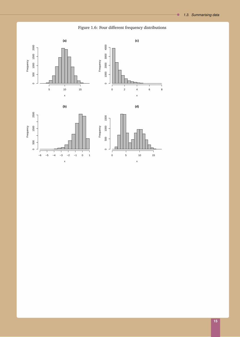
The histograms in Fig. 1.6 show the frequency distributions for four sets of data. We notice that for Fig. 1.6(a)-(c), there is only one “peak" or “hump". A frequency distribution that displays one peak is called a unimodaldistribution (as opposed to those with more than one peak [Fig. 1.6(d)], which are called multi-modal). Afrequency distribution that is asymmetric [Fig. 1.6 (b), (c)] is called skewed; otherwise, it is called symmetric[Fig. 1.6 (a)]. For a unimodal distribution that is symmetric, Sample mean ≈ sample mode ≈ sample median.
14
1.3. Summarising data
Figure 1.6: Four different frequency distributions
(a)
x
Fre
quen
cy
5 10 15
050
010
0015
0020
00
(b)
x
Fre
quen
cy
−6 −5 −4 −3 −2 −1 0 1
050
015
0025
00
(c)
x
Fre
quen
cy
0 2 4 6 8
010
0020
0030
0040
00(d)
x
Fre
quen
cy
0 5 10 15
050
010
0015
00
15

2Basic Probability
2.1 Randomness and probability
A pandemic is hitting a region, two different drugs, A and B, are dispatched to the region. One hundredpatients are given A and another 100 patients are given B. Out of those given A, 60 recovered. Of thosegiven B, 70 recovered. A mother is taking her affected child for treatment. Which treatment should she askfor her child? The mother in this example is one of the many situations in life when we have to deal withuncertainties. In those situations, the concept of probabilitya can be very useful in helping us to form ourdecisions.
Let us take a closer look at the pandemic example. Consider the data from those who have been treatedwith A. If we use 1 for “recovered" and 0 for “not recovered", the data would look like the following:
1 1 1 0 0 0 1 1 1 0 0 1 0 1 0 0 1 1 1 11 1 1 0 1 1 0 0 1 1 1 1 0 1 1 0 0 1 1 00 1 0 1 1 0 1 0 0 1 1 1 1 0 1 0 1 1 1 01 0 1 0 1 1 0 0 0 0 1 1 1 0 1 0 0 0 1 11 0 1 1 1 1 0 0 1 1 1 1 0 1 0 0 1 0 1 1
In total, there are 60 1’s (recovered) and 40 0’s (not recovered). We may observe that the outcome of patientsvary, some are successfully treated (1) while some are not (0). Hence, if the treatment is to be given to thechild, we could not say with certainty what the outcome would be: whether the child would get 1 (recovered),or 0 (not recovered). Similarly, for patients given B, there are 70 1’s (recovered) and 30 0’s (not recovered) thatappear in some haphazard order. We call these phenomena, that the 1’s and 0’s appear in some unpredictablemanner, random. A concept that is useful for explaining randomness is probability. This concept can beillustrated through the following example:
Example 2.1
Assume we have a fair coin, such that it is equally likely we would observe heads (H) or tails (T) when the coin is tossed.If we tossed this fair coin, we might observe the following outcomes in the respective tosses:
Toss 1 2 3 4 5 6 7 8 9 · · ·Outcome H T H T T H T H T · · ·
aSometimes also loosely referred to as chance
16
2.2. Proportion and probability
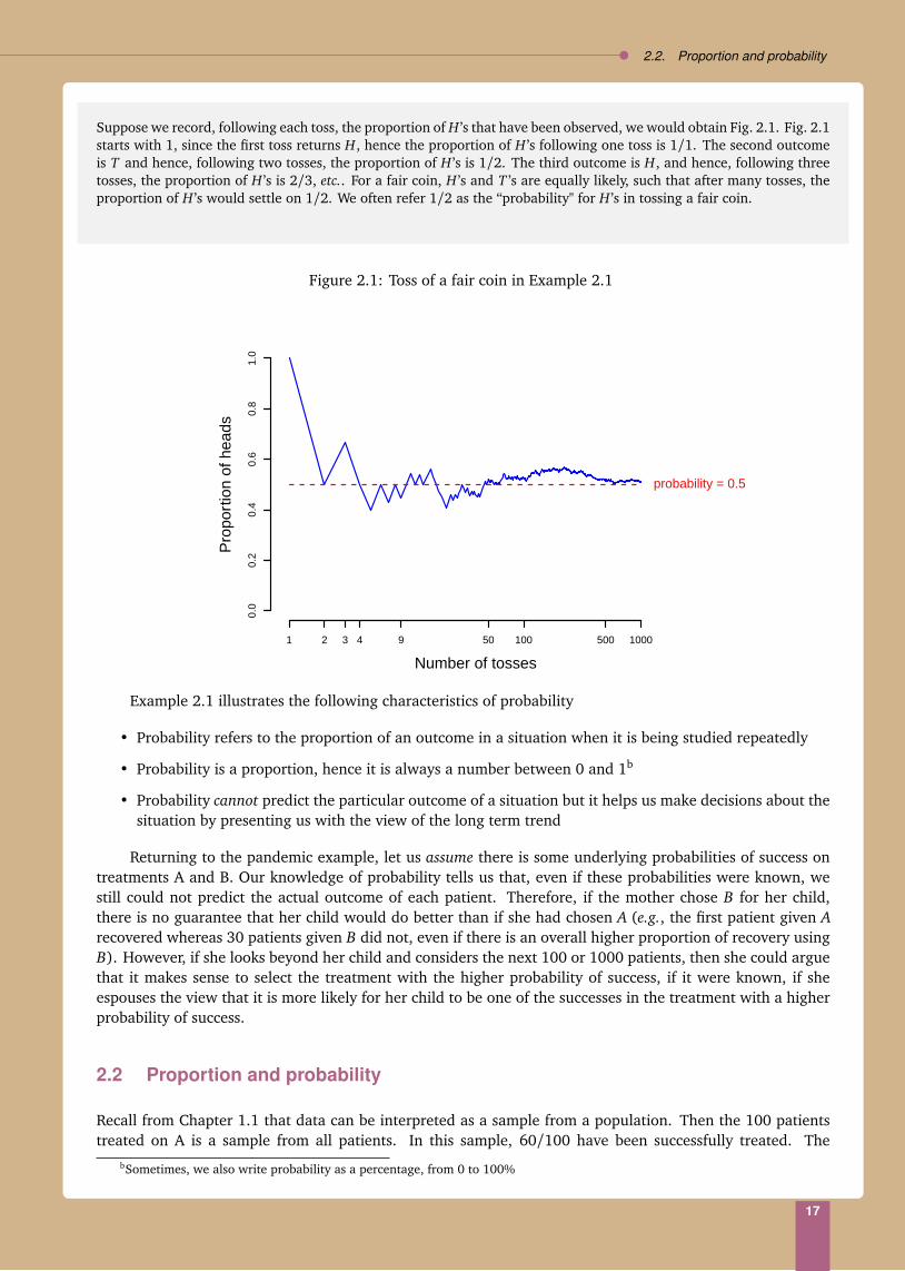
Suppose we record, following each toss, the proportion of H ’s that have been observed, we would obtain Fig. 2.1. Fig. 2.1starts with 1, since the first toss returns H, hence the proportion of H ’s following one toss is 1/1. The second outcomeis T and hence, following two tosses, the proportion of H ’s is 1/2. The third outcome is H, and hence, following threetosses, the proportion of H ’s is 2/3, etc.. For a fair coin, H ’s and T ’s are equally likely, such that after many tosses, theproportion of H ’s would settle on 1/2. We often refer 1/2 as the “probability" for H ’s in tossing a fair coin.
Figure 2.1: Toss of a fair coin in Example 2.1
Pro
port
ion
of h
eads
0.0
0.2
0.4
0.6
0.8
1.0
1 2 3 4 9 50 100 500 1000
probability = 0.5
Number of tosses
Example 2.1 illustrates the following characteristics of probability
• Probability refers to the proportion of an outcome in a situation when it is being studied repeatedly
• Probability is a proportion, hence it is always a number between 0 and 1b
• Probability cannot predict the particular outcome of a situation but it helps us make decisions about thesituation by presenting us with the view of the long term trend
Returning to the pandemic example, let us assume there is some underlying probabilities of success ontreatments A and B. Our knowledge of probability tells us that, even if these probabilities were known, westill could not predict the actual outcome of each patient. Therefore, if the mother chose B for her child,there is no guarantee that her child would do better than if she had chosen A (e.g., the first patient given Arecovered whereas 30 patients given B did not, even if there is an overall higher proportion of recovery usingB). However, if she looks beyond her child and considers the next 100 or 1000 patients, then she could arguethat it makes sense to select the treatment with the higher probability of success, if it were known, if sheespouses the view that it is more likely for her child to be one of the successes in the treatment with a higherprobability of success.
2.2 Proportion and probability
Recall from Chapter 1.1 that data can be interpreted as a sample from a population. Then the 100 patientstreated on A is a sample from all patients. In this sample, 60/100 have been successfully treated. The
bSometimes, we also write probability as a percentage, from 0 to 100%
17

Chapter 2. Basic Probability
number, 60/100, refers to a sample proportion, which must be distinguished from the underlying probabilityof being successfully treated on A, for all patients in the population. A probability is always associated with apopulation; it is the (population) proportion of patients who are successful treated, out of all patients in thepopulation.
Example 2.2 (Continued from Example 2.1)
If we use data from the first nine tosses of our coin, we have
Toss 1 2 3 4 5 6 7 8 9Outcome H T H T T H T H T
which gives a (sample) proportion of 4/9 of H’s. The figure P(H) = 0.5 for this coin refers to the proportion of H’s thatwould have been obtained, if the coin is tossed many times. Hence, the outcomes of the many tosses is a population ofoutcomes, whereas those of the nine tosses is a sample.
Example 2.3
A university has 143 professors and among them, 55 are female and 88 are male. If we pick a professor at random, thenthe probability of picking a female is the same as the proportion of female professors, 55/143. Similarly, the probabilityof picking a male professor is 88/143. In this case, the 143 professors represent all the professors in the university, as suchit is the population of interest. The quantities 55/143 and 88/143 are population proportions, and hence probabilities.
Suppose we randomly select 6 professors, and their gender are:
F F F M M F
Then our data come from a sample and in our sample, the (sample) proportion of female is 4/6, which is different fromthe probability of 55/143. Similarly, the sample proportion of male professors is 2/6, compared to the probability ofmale professors, which is 88/143.
In this example, we also encounter the concept of randomness, genders in the data do not seem to follow any predictablepattern, and hence, random. Furthermore, even though the probability of a female professor is lower at the university,for this particular sample of six professors, there are actually more females than males.
2.3 Terminologies, rules and axioms
For us to effectively use probability to explain randomness, it would be useful for us to learn someterminologies, rules and axioms.
In any situation we are studying, we might be interested in a particular outcome or a collection ofoutcomes. A general term for an outcome or a collection of outcomes is called an event.
Example 2.4
Suppose we have a die, marked 1, 2, 3, 4, 5, and 6. Then the possible outcomes when the tie is tossed is one of the sixnumbers. If we are interested in odd numbers, then we are interested in the event, say A, such that A= 1, 3,5. On thehand, if we are going to toss the die twice, and we are interested in obtaining two 6’s, then the event of interest wouldbe A= 6,6.
If we are interested in an event A, then we use the notation P(A) to denote the “probability that A occurs".Probabilities are numerical values. We attach numerical values to probabilities so we can
18

2.3. Terminologies, rules and axioms
• Compare the probabilities between different events, e.g., Let A = recovery given A, B = recovery givenB in the pandemic example, then P(A) = 0.6, P(B) = 0.7, therefore P(B)> P(A).
• Carry out calculations on probabilities
The following are some basic rules of probability:
Rule 1: For any event A, the probability P(A) is a number between 0 and 1. That is 0 ≤ P(A) ≤ 1. If P(A) = 0,then we mean that we are certain that A will not occur. If P(A) = 1, then we are certain that A will occur.In most cases, we are interested in events with probabilities other than these two extremes.
Example 2.5Suppose we are interested in the weather for tomorrow and the possible outcomes are: “Rain" or “No rain". Then0≤ P(Rain)≤ 1 and 0≤ P(No rain)≤ 1.
Rule 2: In any situation, if S represents the set of all possible outcomes, then P(S) = 1.
Example 2.6In Example 2.5, there are only two possible outcomes: “Rain" or “No rain", hence S= rain, no rain.P(S) = 1.
Rule 3: If A is an event, then the event A does not occur is the complement of A, denoted by Ac or A. For anyevent A with probability P(A), the probability that A does not occur is P(Ac) = 1− P(A).
Example 2.7In Example 2.5, if A=No rain, then Ac=Rain and P(No rain) = 1− P(Rain).
Rule 4: If there are two events, A and B, then the joint probability between A and B are defined as the probabilityof occurrence of both A and B, written as
P(A and B)≡ P(A∩ B).
The two events are disjoint or mutually exclusive if they cannot happen simultaneously, in which case
P(A∩ B) = 0.
Example 2.8In Example 2.5, let A=No rain and B=Rain. Since it either rains or it does not rain, A and B are mutuallyexclusive events,
P(Rain and No rain) = 0.
19

Chapter 2. Basic Probability
Rule 5: (Multiplication Rule) If A and B are two events, then
P(A and B) = P(B)× P(A|B).
Here, P(A|B) is called the conditional probability of A given B.
Example 2.9If two cards are selected at random, one at a time without replacement (the first card drawn is not put back inthe deck) from a deck of 52 cards, what is the probability that both cards will be aces?Let A=First card is an ace and B =Second card is an ace
P(Two aces) = P(A and B)= P(First card is an ace)× P(Second card is an ace|First is an ace)
=4
52×
351= 0.0045
Rule 5a: (Conditional probability) Rearranging the multiplication rule gives
P(A|B) =P(A and B)
P(B),
which is a general expression for calculating conditional probabilities.
Example 2.10In a class of 105, 40 students are female, and among the female students, 10 are foreigners. What is the probabilitythat a female student is a foreigner?Let A=Foreign and B =Female
P(Foreign|Female) = P(A|B)
=P(A and B)
P(B)
=P(Female foreign student)
P(Female)
=10/10540/105
= 0.25.
Rule 6: (Independent events) Two events A and B are independent if knowing whether A occurred does notchange the probability that B occurs, and vice versa. If two events A and B are independent, then
P(A|B) = P(A) and P(B|A) = P(B).
The above equalities make sense. For example, P(B|A)means the probability of B given A. If A and B areindependent, then knowing A does not change the probability that B happens. Therefore, the probabilityof B given A must be the same as P(B) without any knowledge of whether A occurred or not.
For independent events A and B,P(A∩ B) = P(A)P(B)
20

2.3. Terminologies, rules and axioms
Example 2.11If two cards are selected at random, one at a time with replacement (so that the first card is put back in the packbefore the second is selected) from a pack of 52 cards, what is the probability that both cards are aces?
P(Two aces) = P(First is an ace and second is an ace)= P(First is an ace)× P(Second is an ace)
=4
52×
452= 0.0059.
Since the first card is returned to the pack, the probability that the second is also an ace is exactly the same as thatfor the first card. In this case, the events, A=First card is an ace and B=Second card is an ace are independent.
Rule 7: Total Probability (Union of events):
If A and B are not disjoint, then
P(A or B)≡ P(A∪ B) = P(A) + P(B)− P(A and B).
If A and B are disjoint, then P(A and B) = 0, therefore,
P(A or B) = P(A) + P(B)
In probability, “or" means “at least one of" so A∪ B includes A, B or both A, B.
Example 2.12If a fair die (a die such that the probabilities of observing any one of the six numbers are the same, i.e., 1/6) isrolled twice, what is the probability of getting at least one 6? This is the same as asking for
P(6 on first roll or 6 on second roll or 6 on both rolls),= P(6 on first roll) + P(6 on second roll)− P(6 on both rolls)
=16+
16−
16×
16
=1136
In this example, A is the event 6 on first roll and B is the event 6 on second roll. For P(6 on both rolls), weused the multiplication law for independent events.
Example 2.13In Example 2.5, since A=Rain and B=No rain are mutually exclusive, hence P(A∩ B) = 0 and consequently,
P(Rain or No rain) = P(A∪ B) = P(A) + P(B).
Rule 8: Complementary events and the calculation of P(At least 1)
Under the complementary rule, P(A) = 1 − P(Ac). If we are interested in the event A=At least one,then the complement event is Ac=None; furthermore,
P(At least 1)= 1− P(None)
21

Chapter 2. Basic Probability
Example 2.14For families of four children, what is the probability that there will be at least one boy, assuming boys (B) andgirls (G) are equally likely and births are independent?Instead of listing the 16 outcomes BBBB, BBBG, etc., we simply use
P(At least one boy) = 1− P(No boys)= 1− P(GGGG)
= 1−12×
12×
12×
12
=1516
.
Rule 9: Often, it is given P(A|B) but the interest is in P(B|A), Bayes Theorem provides a solution:
P(A|B) =P(B|A)P(A)
P(B)
Example 2.15Among three airlines providing services between two cities, airline A has 50% of all the scheduled flights, airlineB has 30% and airline C has 20%. Their on-time departure rates are 80%, 65% and 40%, respectively. A planehas just departed on time. What is the probability that it was airline A?Let D =on time, A=airline A, B =airline B, C =airline C. Then:
P(A) = 0.5,P(B) = 0.3, P(C) = 0.2, P(D|A) = 0.8, P(D|B) = 0.65,P(D|C) = 0.4
P(D) = P(D|A)P(A) + P(D|B)P(B) + P(D|C)P(C)= 0.4+ 0.195+ 0.08= 0.675
P(A|D) =P(D|A)P(A)
P(D)=
0.40.675
= 0.593
Rule 10: Partition rule
For any A, a partition is any collection of disjoint subsets of A that together make up A; P(A) can bewritten as the sum of the probabilities of its disjoint subsets.
Example 2.16If A= all white women, a partition of A is A1 =all white women with wage < 3 and A2 =all white womenwith wage ≥ 3. Hence:
P(A) = P(A1) + P(A2)
22

2.4. Probability tree
Figure 2.2: Probability tree for two independent tosses of a fair coin
Toss 1
Toss 2
P(H ∩H) = 12 ·
12
H12
P(H ∩ T ) = 12 ·
12T
12
H12
Toss 2
P(T ∩H) = 12 ·
12
H12
P(T ∩ T ) = 12 ·
12T
12
T12
Figure 2.3: A typical probability tree that records conditional probabilities
Event 1
Event 2
E1
P(E1)
Event 2
Event 3
P(E1 ∩ E2 ∩ E3)
E3
P(E3|E1 ∩ E2)
P(E1 ∩ E2 ∩ E3)E3
P(E3|E1 ∩ E2)E2
P(E2|E1)E1
P(E1)
2.4 Probability tree
Probability tree is a useful way to visualize probabilities when we are dealing with combinations of events.Each branch in a probability tree represents a possible outcome. If two events are independent, the outcomeof one has no effect on the outcome of the other. For example, if we toss two coins, getting heads with thefirst coin will not affect the probability of getting heads with the second. A probability tree which representsa coin being tossed two times, assuming toss outcomes are independent looks like Fig. 2.2.
Notice the probabilities on the branches are conditional probabilities. Therefore, a probability tree is agood candidate for carrying out calculations that involve conditional probabilities. For example, from the treejust given, P(H ∩ H) = P(H in second toss|H in first toss)P(H in first toss) = (1/2)(1/2) since the two tossesare independent.
A tree can have many branches. For example, for three events, the tree would look like Fig. 2.3. Noticethat P(E1 ∩ E2 ∩ E3) = P(E1)P(E2|E1)P(E3|E1 ∩ E2). In general, if there are K events, then P(E1 ∩ · · · ∩ EK)can be evaluated by multiply all the probabilities along the path back to the root of the tree, which isP(E1)P(E2|E1) · · ·P(EK |E1 ∩ · · · ∩ EK−1).
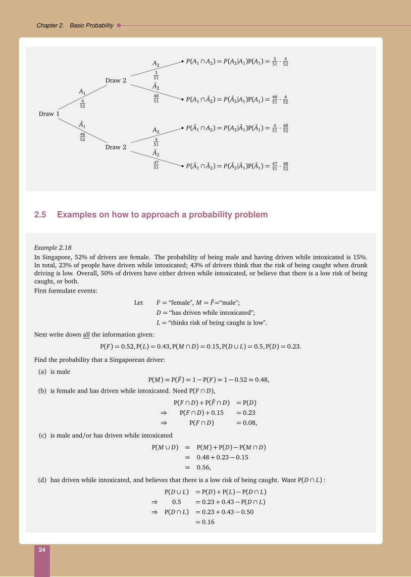
Example 2.17 (Continued from Example 2.9)
Let Ai denote "Ace is drawn" in i-th draw, i = 1,2. The two draws can be represented as:
23
Chapter 2. Basic Probability
Draw 1
Draw 2
P(A1 ∩ A2) = P(A2|A1)P(A1) =4751 ·
4852
A2
4751
P(A1 ∩ A2) = P(A2|A1)P(A1) =451 ·
4852A2
451
A1
4852
Draw 2
P(A1 ∩ A2) = P(A2|A1)P(A1) =4851 ·
452
A2
4851
P(A1 ∩ A2) = P(A2|A1)P(A1) =351 ·
452A2
351
A1
452
2.5 Examples on how to approach a probability problem
Example 2.18In Singapore, 52% of drivers are female. The probability of being male and having driven while intoxicated is 15%.In total, 23% of people have driven while intoxicated; 43% of drivers think that the risk of being caught when drunkdriving is low. Overall, 50% of drivers have either driven while intoxicated, or believe that there is a low risk of beingcaught, or both.First formulate events:
Let F = “female", M = F=“male";
D = “has driven while intoxicated";
L = “thinks risk of being caught is low".
Next write down all the information given:
P(F) = 0.52,P(L) = 0.43,P(M ∩ D) = 0.15, P(D ∪ L) = 0.5,P(D) = 0.23.
Find the probability that a Singaporean driver:
(a) is maleP(M) = P(F) = 1− P(F) = 1− 0.52= 0.48,
(b) is female and has driven while intoxicated. Need P(F ∩ D),
P(F ∩ D) + P(F ∩ D) = P(D)⇒ P(F ∩ D) + 0.15 = 0.23
⇒ P(F ∩ D) = 0.08,
(c) is male and/or has driven while intoxicated
P(M ∪ D) = P(M) + P(D)− P(M ∩ D)= 0.48+ 0.23− 0.15
= 0.56,
(d) has driven while intoxicated, and believes that there is a low risk of being caught. Want P(D ∩ L) :
P(D ∪ L) = P(D) + P(L)− P(D ∩ L)⇒ 0.5 = 0.23+ 0.43− P(D ∩ L)⇒ P(D ∩ L) = 0.23+ 0.43− 0.50
= 0.16
24

2.5. Examples on how to approach a probability problem
(e) has driven while intoxicated, and believes that the risk of being caught is not low. Want P(D ∩ L):
P(D ∩ L) + P(D ∩ L) = P(D)⇒ 0.16+ P(D ∩ L) = 0.23
⇒ P(D ∩ L) = 0.23− 0.16
= 0.07
(f) is male given the person is intoxicated. Want P(M |D):
P(M ∩ D)P(D)
=0.150.23
= 0.65.
Example 2.19
Probabilities from tables of counts. The following table gives the number of applicants to SMU in 2003, classified by sexand SAT score:
SexMale Female Total
< 800 79 13 92SAT 800-1000 772 216 988
1000-1150 1081 499 1580>1150 1795 2176 3971Total 3727 2904 6631
Let event A=“applicant is female", B=“applicant’s SAT < 800".
(a) Suppose a person is chosen at random from the table:
P(A) = P(female) =No. of female applicantsTotal no. of applicants
=29046631
= 0.44.
Notice in this case, the table represent the entire population of applicants to SMU in 2003, hence, probability is givenby the (population) proportion, see Chapter 2.2 and Example 2.3.
(b) But, if only people from those with SAT < 800 are chosen, then:
P(Applicant is female, given SAT< 800) = P(A|B)
=P(A∩ B)
P(B)
=no. female applicants with SAT< 800total no. applicants with SAT< 800
=1392= 0.14.
(c) Are A and B independent?
Two ways to prove independence: (i) A and B are independent if and only if
P(A∩ B) = P(B)P(A).
Using the table of frequencies,
P(A∩ B) =13
6631= 0.00196,
P(A) =29046631
= 0.4379,
P(B) =92
6631= 0.01387.
So,P(A)P(B) = 0.4379× 0.01387= 0.00607 6= P(A∩ B).
25

Chapter 2. Basic Probability
Not independent! (ii) A and B are independent if P(A|B) = P(A) and P(B|A) = P(B). From above P(A|B) = 0.14, butP(A) = 0.4379, therefore, P(A|B) 6= P(A). Not independent!
(d) What is the probability that the applicant is female or the applicant’s SAT is above 800?
Want P(A∪ B) = P(A) + P(B)− P(A∩ B).P(B) = 1−P(B) = 1− 92
6631 = 0.986. Since A and B are not independent, A and B are also not independent. So to obtainP(A∩ B), we must look at the entries in the table and not use P(A)P(B). P(A∩ B) = 216+499+2176
6631 = 0.436.
SoP(A∪ B) = 0.44+ 0.986− 0.436= 0.99.
Make sure all probability calculations give an answer between 0 and 1! (Rule 1)
26

3Univariate distributions
3.1 Random variables and distributions
In the pandemic example in Chapter 2, we were interested in the treatment outcome for someone affectedby a disease. We noticed that even for patients treated on the same drug, some recovered and some did not.Furthermore, the treatment outcome for future patients could not be predicted precisely. We called such aphenomenon “random". Whenever we are studying a variable, such that its value varies randomly betweenobservations, we call the variable a random variable. Hence, treatment outcome is a random variable. Thereare many other examples of random variables. In Example 1.3 of Chapter 1, we have records of seven variablesfrom a group of students. Not only the values of each variable vary over students, if we randomly select anotherstudent from the same school, it would not be possible to predict the student’s gender, GPA, etc. Hence, thevariables in Example 1.3 are random variables.
A random variable may take any value from a set of possible values. For example, in the pandemicexample, the possible values of treatment outcome are 1 (recovered) or 0 (not recovered). In Example 1.3,suppose we are interested in Course GPA, the possible values fall in the interval from 0 to 4.3. In either case,even though we know the set of all possible values of the random variable, its value could not be predictedprecisely before we observe the data. Furthermore, some values may be more likely than others to occur. Forexample, it may be more likely for a patient to recover if the patient is given treatment; it may be more likelyto see Course GPA between 2.7 and 3.0 than above 4.0, etc..
Random variables can generally be classified into one of two types: discrete random variables andcontinuous random variables. When the set of possible values a random variable can take is countable, thenthe variable is a discrete random variable. A continuous random variable, on the other hand, can take valuesin a set of uncountable possible values, for example, values in an interval.
Example 3.1 We reproduce the data in Example 1.3 here. In this set of data, Status, Gender, School, Course GPA, CourseGrade are all discrete random variables. Cumulative GPA is a continuous random variable. Age can be considereda discrete random variable if we age rounded to the nearest year, as shown in the table, or it may be considered acontinuous random variable if we use the exact age of each student.
Student Status Gender Age School Course Course CumulativeGPA Grade GPA
1 Singaporean Male 23 SOE 3.7 A- 2.992 Foreign Female 23 SIS 3.7 A- 3.923 Singaporean Female 19 SOA 2.7 B- 3.334 Singaporean Female 20 SOA 4.0 A 3.15
27

Chapter 3. Univariate distributions
5 Singaporean Female 36 SOB 4.3 A+ 3.666 Foreign Male 27 SOB 3.3 B+ 2.677 Singaporean Female 23 SOS 3.3 B+ 2.988 Foreign Male 25 SOB 2.3 C+ 2.359 Singaporean Male 22 SOB 3.7 A- 3.23
10 Singaporean Female 19 SOE 3.0 B 3.7211 Foreign Male 19 SOB 3.3 B+ 3.7712 Singaporean Male 19 SOA 1.7 C- 2.1713 Foreign Female 18 SOB 4.0 A 3.4214 Singaporean Female 19 SOS 1.7 C- 2.1715 Singaporean Female 18 SOS 4.0 A 3.4216 Singaporean Female 19 SOL 1.7 C- 2.1717 Singaporean Female 18 SOL 4.0 A 3.42
In Chapter 2, we discussed how probability helps us to explain randomness. When we are studying arandom variable, with possible values in a set, but some values are more likely that others to occur, we needa probability distribution. Often a probability distribution is simply referred as a distribution. A distributionrecords the probabilities for the occurrence of the different values of a random variable. In other words, adistribution is simply a collection of probabilities, one for each of the outcomes of a random variable.
There are two main types of distributions: discrete distribution and continuous distribution, for eachof the two main types of random variables.
3.2 Discrete distributions
3.2.1 Introduction to discrete distributions
When we toss a coin with two faces, if the coin is fair and the chance that the coin would land on its edgeis practically zero, then the toss outcome is a random variable, say X , with two possible values: H (heads)or T (tails). Since there are two possible values of X , hence countable, X is a discrete random variable. Theprobability of H, P(X = H) ≡ P(H) = 1/2 and the probability of T , P(X = T ) ≡ P(T ) = 1/2. In this case,we have an example of a distribution of one toss of a fair coin. A distribution tells us the probabilities of allthe outcomes in the toss of a coin. In this case, we have only two possible outcomes and each outcome has aprobability 1/2 of occurring. We can also represent the probability distribution in the form of a table
Outcome ProbabilityH (heads) 1/2T (tails) 1/2
We notice from the table that the probabilities of the two possible outcomes sum to 1.
Example 3.2Consider rolling a die with six faces: 1, 2, 3, 4, 5, 6.
distribution for the outcome of the roll of a die
Outcome 1 2 3 4 5 6
Probability 16
16
16
16
16
16
28

3.2. Discrete distributions
In this case, there are six possible outcomes, hence countable and discrete. The distribution tells us that the six outcomesare equally probable. Once again, the probabilities of all the possible outcomes sum to 1.
Example 3.3
Consider tossing a fair coin three times and counting the number of heads in the three tosses. We assume that theoutcome of each toss is independent of each other. In Chapter 2, we talked about the concept of independent events.This means, in the current context, the outcome of one toss is not dependent on the outcomes of previous (and future)tosses. Let us enumerate the different possible outcomes from three tosses of a coin. The possible outcomes are (H =heads, T = tails):
HHH, HHT, HT H, T HH, HT T, T HT, T T H, T T T
What is the probability of each of these outcomes? Let us look at the outcome HHH. Since P(H) = P(T ) = 1/2 in onetoss of a fair coin, the probability of observing the first H is 1/2. Subsequently, the probability of obtaining HH, by theindependence assumption and using the multiplication rule for independent events, P(HH) = P(H)P(H) = (1/2)(1/2).Similarly, the probability of obtaining HHH is P(HHH) = P(H)P(H)P(H) =(1/2)(1/2)(1/2) = (1/2)3.
We can use the same argument for the outcome HHT , P(HHT ) = P(H)P(H)P(T ) = (1/2)(1/2)(1/2) = (1/2)3. Theprobabilities for the other outcomes are similarly determined to be (1/2)3.
Now, we are only interested in the number of heads. If the three tosses give HHH, then the total number of heads is 3.Therefore, P(3 heads) = P(HHH) = (1/2)3 =0.125.
On the other hand, any of the three outcomes HHT , HT H, or T HH would give 2 heads. Therefore, P(2 heads) =P(HHT, HT H or T HH) = P(HHT ) + P(HT H) + P(T HH) = 3(1/2)3 = 0.375.
Similarly, any of the three outcomes HT T , T HT , T T H would give 1 head. Therefore, P(1 head)=P(HT T, T HT or T T H) = 3(1/2)3 = 0.375.
Finally, if the three tosses are T T T , then the number of heads is 0. Therefore, P(0 heads) = P(T T T ) = (1/2)3 = 0.125.
Summarizing the calculations, we have
Table 3.1: distribution for the number of heads in three tosses of a coin
Number of heads Probability0 (1/2)3 = 0.1251 3(1/2)3 = 0.3752 3(1/2)3 = 0.3753 (1/2)3 = 0.125
Once again, the probabilities of the different outcomes sum to 1.
The distribution can also be depicted in a graph, see Fig. 3.1. The graph of a discrete distribution is normalised so thatthe height of each bar is equal to its area, both of which represent probability. For example, in Fig. 3.1, the area (orheight) of each bar in the graph gives the probability of the outcome, hence, the areas (heights) of the four bars sum to1.
In this example, even though we know all the possible values of outcome, the actual outcome, is unknown until thecoins are tossed. As such, the outcome is a random variable. In addition, the random variable is discrete because thenumber of possible outcomes is countable: 0, 1, 2, or 3 heads. “The number of heads" is random because we wouldnot know its value until the coins are tossed. Nevertheless, the distribution gives us some idea of the relative chancesof the different outcomes. The situation is analogous to the example at the beginning of Chapter 2, where the motherbelieves treatment B gives a higher chance of recovery for her child, even though she would not find out whether herchild would recover until after the treatment is given. Therefore, a random variable is a term for the unknown outcomeof any situation that we may be interested in.
29

Chapter 3. Univariate distributions
Figure 3.1: distribution of the number of heads in three tosses of a fair coin
0 1 2 3
Number of heads
Pro
babi
lity
0.0
0.2
0.4
0.6
0.8
3.2.2 Properties of a discrete random variable
Based on the examples in Chapter 3.2.1, we now formally define a discrete random variable and give itsproperties.
A discrete random variable, X , is used to describe the unknown outcome of a situation if the value of Xcan only come from a countable number of possible values: a1, a2, ..., ak, where k is any positive integer ≥ 2.Some possible cases are illustrated in the following example:
Example 3.4
• Treatment outcome: X = 1 or 0 (2 possible values)
• Die: X = 1, 2, 3, 4, 5 or 6 (6 possible values)
• Three tosses of a fair coin : X = HHH, HHT, HT H, T HH, HT T, T HT, T T H, T T T (8 possible values)
• No. of infections in a large population: X = 0, 1, 2, 3,... (Large and possibly infinite but countable number ofpossible values)
P(X = ai) is called a probability distribution function (often abbreviated as pdf or PDF); it gives theprobability that X = ai . The probability distribution function, or simply distribution function, tells us howlikely the different outcomes of a discrete random variable occur. A valid distribution function must satisfythe following rules:
• P(X = ai) must be between 0 and 1, i.e., the probability of each outcome must be non-negative.Furthermore, the proportion of times an outcome appears cannot be more than 1.
• We are certain that one of the outcomes would appear:
P(X = a1 or X = a2 or ... or X = ak) = 1.
Furthermore, since X cannot assume two outcomes simultaneously, the k outcomes are mutuallyexclusive. Therefore, by the total probability rule in Chapter 2.3:
P(X = a1 or X = a2 or ... or X = ak) = P(X = a1) + P(X = a2) + ...+ P(X = ak) = 1,
30

3.2. Discrete distributions
which means the sum of the probabilities of all the outcomes is 1.
Example 3.5 (Continued from Example 3.3)
There are four distinct outcomes: 0, 1, 2, 3. Let X = “the number of heads in three tosses".
P(X = 0) = 0.125 > 0
P(X = 1) = 0.375 > 0
P(X = 2) = 0.375 > 0
P(X = 3) = 0.125 > 0
P(X = 0, 1, 2 or 3) = 0.125+ 0.375+ 0.375+ 0.125 = 1. This last statement is true, because, even though before thetosses we would not know whether 0, 1, 2, or 3 H ’s appear, it is certain one of these four outcomes must appear, hencethe probability is 1.
The distribution of a discrete random variable can be presented as a table, as in Table 3.1, or as a picture,as in Fig. 3.1. There is a third way of representing a discrete distribution that we will explore in Chapter 6.
3.2.3 Distributions as models
At the beginning of Chapter 1, we talked about the two goals of a statistical analysis, making sense of the dataand generalising what is observed in the data to the population of interest. Here, we discuss how these twogoals can simultaneously be achieved using distribution as a model for the data.
In Example 2.2, a fair coin is tossed nine times to yield a set of data. Earlier, we talked about how datacan be interpreted as sample from a population, so in this context, we have a sample of nine outcomes, outof the many outcomes if this coin were tossed many times (the population of toss outcomes). In other words,the nine outcomes is a subset of the many possible outcomes that could have been observed from repeatedtosses of the coin.
The data show that the order of H ’s and T ’s in the nine tosses seems unpredictable. We learned inChapter 2.1 we could use probability to explain such phenomenon. For a fair coin, there are only two possibleoutcomes: H or T . The probabilities for these outcomes are: P(H) = 0.5 and P(T ) = 0.5. We argued theseprobabilities can be interpreted as population proportions (see Chapter 2.2). In other words, if we tossed thecoin many times, half of the outcomes would be H ’s and the remaining T ’s. However, in any single toss, it isnot certain whether H or T would appear; this is the randomness we referred to in the nine tosses. Hence,the two probabilities P(H) = 0.5 and P(T ) = 0.5, which form a distribution (see Chapter 3.2.1) can explainthe nine tosses (the data) as well as the many tosses that have not been made (the population). In this sense,the distribution helps to explain the observation made in the data, and link the data to the population. Wecall the distribution a probability model for the outcome of a coin toss. The probability model explains theoutcomes of the nine tosses and the same model allows us to talk about the “population" of tosses that havenot been made.
Example 3.6
In the pandemic example in Chapter 2, we have data on the outcomes of 100 patients treated on drug A. The outcomesare of only two possible values: 1 (recovered) or 0 (not recovered). In the data, 60 patients are observed to haverecovered while 40 did not recover; the outcomes in these patients do not appear in any particular order.
In order for us to explain the outcomes in the data, and to use the data to infer about the population of all patients,both past and future, we need a probability model. Since there are only two outcomes: 1 or 0, we imagine there is anunderlying distribution for treatment outcome under A, for all patients, including the 100 we have observed and thosewho have not received the treatment. The distribution looks like:
31

Chapter 3. Univariate distributions
Outcome Probability1 (recovered) P(1)
0 (not recovered) P(0)
The distribution links a probability to each of the two possible outcomes. Each probability can be interpreted as apopulation proportion: P(1) tells us the proportion of patients who would recover, among all patients in the populationtreated on A; P(0) is the proportion among all patients in the population who would not recover, even given A. Weassume the distribution (model) gave rise to the data in the 100 patients. The same model would apply to patients whohave not been treated. Hence, if we wish to say something about future patients, we would use P(1) and P(0), so forexample, we can say that, among the population of patients treated on A, a proportion of P(1) would recover.
3.3 Continuous distributions
In Example 1.13 of Chapter 1, we have a set of data from 423 working married white women. The data consistof the women’s hourly wage rate over year 1975, and they look like the following: 3.3540, 1.3889, 4.5455,1.0965, 4.5918, etc.. Hourly wage rate for each woman was calculated based on the woman’s “total wageover 1975" ÷ “number of hours she worked in 1975", and hence, is a real number, as reflected in the data(there was rounding for ease of presentation). Let us use X to denote “hourly wage rate" and let us assumehourly wage rate is never more than b dollars in 1975, then X is a real number with possible values in therange (0, b). According to Chapter 3.2, X is a continuous random variable. Suppose we wish to analyse thisset of data to learn more about X . As we did in Chapter 3.2.3, we can find a distribution (model) for X . Adistribution allows us to describe what is observed in the 423 women. Furthermore, by using the probabilitiesin the distribution, we would be able to say, for example, what proportion in the population of all workingwhite married women have hourly wage rate of say, between 3-5 dollars, etc..
As discussed earlier in Chapter 3.2, a distribution gives a probability for the occurrence of each value ofa random variable. However, for a continuous random variable X , there are uncountably many values thatfall within a range. Hence, it would not be possible to list the probabilities for all possible values of X , likewe did for a discrete random variable. This problem is solved by using a probability density function (oftenabbreviated as pdfa). A probability density function is sometimes simply referred to as a probability densityor a density.
3.3.1 Introduction to continuous distributions
To motivate our discussion of a continuous distribution, we briefly return to the case of a discrete distribution.One of the two ways of presenting a discrete distribution is to use a picture, as in Fig. 3.1. In Fig. 3.1, the areaof each bar equals the probability of observing a particular outcome, and the sum of the areas of the bars is1. For example, the bar for obtaining 2 heads out of three tosses has an area that is 0.375, which is 3 timesthe area for 0 heads out of 3 tosses. For a continuous random variable X , we will use the same idea, i.e., apicture to represent its distribution. This idea is illustrated in Fig. 3.2, which shows the plot of a distributionfor a continuous random variable, X (left panel) and that for a discrete random variable, Y (right panel). Asdiscussed earlier in this section, the distribution for a continuous random variable is described by a densityfunction. If X is a continuous random variable, we often write the density function of X by f (x), where f andx are both lower case letters. In the left panel of Fig. 3.2, the density function f (x) is the black curve, andf (x) means the value of the black curve at X = x . The choice of the letter f is not strict, we could also useother letters, such as g, h, etc..
Observing Fig. 3.2, we can draw a clear correspondence between the density f (x) of the continuous
aNotice that pdf may also mean “probability distribution function", as for a discrete random variable. Hence, we have to rely onthe context to determine the meaning of pdf
32

3.3. Continuous distributions
random variable X and the distribution function P(Y ) of the discrete random variable Y . Both f (x) and P(Y )are non-negative over the respective ranges of the random variables they represent. The total area under f (x)is 1; the sum of areas (heights) of P(Y ) is also 1.
Figure 3.2: distribution of a continuous vs. a discrete random variable
X
Pro
babi
lity
dens
ity fu
nctio
n, f(
x)
X
Pro
babi
lity
dens
ity fu
nctio
n, f(
x)
0
Total area = 1
Y
Pro
babi
lity
dist
ribut
ion
func
tion,
P(Y
)
0
Total area = 1
To find probability for a discrete random variable Y , we simply add up the area(s) of the barscorresponding to the values of Y we are interested in. For example, if we wish to find P(Y = 1 or 2) = P(Y =1) + P(Y = 2), we add up the areas under Y = 1 and Y = 2. The same idea is used to find probabilities for acontinuous random variable X , except the mechanics are different. Suppose we wish to find P(x ≤ X ≤ x+d x),for d x > 0 (Another way of writing this is PX ∈ (x , x + d x)). So we are interested in the probability of Xin the interval (x , x + d x). Following what we did with a discrete random variable, we find the area of f (x)under (x , x + d x). This probability is depicted as the shaded region in Fig. 3.3.
Figure 3.3: Finding probabilty of a continuous random variable
Pro
babi
lity
dens
ity fu
nctio
n, f(
x)P
roba
bilit
y de
nsity
func
tion,
f(x)
0
x x + dx
When d x is small, the shaded area, PX ∈ (x , x + d x), would look like the area of a rectangle, withwidth d x and height ≈ f (x). Using this idea, P(X = x) ≡ PX ∈ (x , x + d x), d x = 0, is given by a rectanglewith width d x = 0 and height = f (x), which has an area of exactly 0. Hence, for any continuous randomvariable X , P(X = x) = 0 for any value of x . This aspect of a continuous random variable is different from adiscrete random variable. Since P(X = x) = 0 but f (x) ≥ 0 over the range of X , therefore, f (x) 6= P(X = x).
33

Chapter 3. Univariate distributions
In fact, f (x) is not a probability. For a continuous random variable, we cannot talk about its probability at asingle point because that value is always 0; we can only find its probability over an interval.
We summarise the properties of a continuous distribution next.
3.3.2 Properties of a continuous random variable
A continuous random variable, X , is a random variable with outcome that falls within the range, (a, b),−∞≤a < b ≤∞. If X is a continuous random variable, then there are uncountably many possible values for X .
Example 3.7
Examples of a continuous random variable:
• X = weight of a baby: (a, b) = (0,10) kg
• X = change in the temperature: (a, b) = (−20,20) degrees
• X = time to the next financial crisis: (a, b) = (0,∞) days (years)
For a continuous random variable X , the probability at any single point is exactly 0, hence P(X = x)≡ 0for any value x . Its distribution is described by a (probability) density function, f (x), with the followingproperties:
• f (x)
≥ 0 x ∈ (a, b)= 0 x /∈ (a, b)
• Since f (x) is non-negative, and P(X = x) = 0 for any value of x ∈ (a, b),
f (x) 6= P(X = x)
• Since P(X = x) = 0 for any x; then, for any interval (c, d) ⊆ (a, b),
P(c ≤ X ≤ d) = P(X = c)︸ ︷︷ ︸
=0
+P(c < X < d) + P(X = d)︸ ︷︷ ︸
=0
= P(c < X < d)
Hence, ≤ and < are interchangeable, so are ≥ and >, when calculating probability for a continuousrandom variable. For the same reason, there is no need to distinguish between (c, d) and [c, d], where“[", “]" usually suggest including the end points in an interval
• f (x) is not a probability; the area under f (x) over the interval (c, d) ⊆ (a, b) is a probability
• Since X is known to fall within (a, b), the total area under f (x) over (a, b) is 1
In Chapter 3.3.1, the probability of a continuous random variable was defined as the area under a densityfunction. We now illustrate how to find that area using a technique called integration, see Appendix B.
Example 3.8
Suppose X is a continuous random variable, such that X ∈ (0, 1). Its density function, f (x), is shown in Fig. 3.4, andwe wish to find P(0.5 ≤ X ≤ 0.7), which is given by the shaded area. We observe that f (x) ≥ 0,∀x ∈ (0,1), as arequirement to be a valid density. The density is actually drawn using f (x) = 6x(1− x), x ∈ (0,1).
34

3.3. Continuous distributions
To find the shaded area, we write
PX ∈ (0.5,0.7) =
∫ 0.7
0.5
f (x)d x
=
∫ 0.7
0.5
6x(1− x)d x
=
∫ 0.7
0.5
(6x − 6x2)d x
=
6x2
2− 6
x3
3
0.7
0.5
=
3x2 − 2x30.7
0.5
=
3(0.7)2 − 2(0.7)3
−
3(0.5)2 − 2(0.5)3
= 0.784− 0.5
= 0.284
Figure 3.4: Graph of the pdf of Example 3.8, f (x) = 6x(1− x)
Pro
babi
lity
dens
ity fu
nctio
n, f(
x)
X
Pro
babi
lity
dens
ity fu
nctio
n, f(
x)
0
0 0.5 0.7 1
Example 3.9
Suppose X is a continuous random variable, such that X > 0, with density function, f (x) shown in Fig. 3.5, and we wishto find P(X ≤ 1), which is the shaded area. Once again, f (x) is non-negative over its range; in this case, (0,∞). Thedensity is actually drawn using f (x) = e−x , x ∈ (0,∞).
35

Chapter 3. Univariate distributions
We will find the shaded area as follows,
PX ∈ (0, 1) =
∫ 1
0
f (x)d x
=
∫ 1
0
e−x d x
=
−e−x1
0
=
−e−1
−
−e−0
= −0.3678794− (−1)= 0.6321206
≈ 0.63
Figure 3.5: Graph of the pdf of Example 3.9, f (x) = e−x
Pro
babi
lity
dens
ity fu
nctio
n, f(
x)
X
Pro
babi
lity
dens
ity fu
nctio
n, f(
x)
0
0 1
3.3.3 Cumulative distribution function
For a continuous random variable X , calculating probability about X requires finding an area under its densityf (x). We learned in Examples 3.8 and 3.9 finding an area using integration, see, Appendix B.
In practice, our interest in X might vary for different problems. For example, suppose X represents thehourly wage rate in Example 1.13 of Chapter 1. If we are interested in the proportion of women who earnedless than minimum wage, then we would like to find P(X < minimum wage). On the other hand, if we wishto study women who earned more than the average hourly wage, then we need P(X > average hourly wage),etc.. For each of these questions, we could follow the processes in Examples 3.8 and 3.9 to find the probabilityof interest. However, it would be useful to find a more convenient way of finding probabilities, without theneed to repeat the effort every time we want to study X .
For a continuous random variable X with density f (x) over the range (a, b), the cumulative distributionfunction (often abbreviated as cdf or CDF) is defined as
F(x) = P(X ≤ x) =
∫ x
af (x)d x =
∫ x
−∞f (x)d x .
36

3.3. Continuous distributions
That is, F(X ) is the probability that X takes any value no more than x . Notice that in the definition above,the last two integrals give the same value, because f (x) is zero in (−∞, a) so adding it does not change theresult. The last expression is sometimes used for convenience. There is a one-to-one correspondence betweena pdf and its cdf, as such, we always use the same letter, lower case for pdf, and upper case for cdf.
Example 3.10 (Continued from Example 3.9).
The cdf for a random variable with pdf f (x) = e−x , x ∈ (0,∞), is the following:
F(x) = P(X ≤ x) =
∫ x
0
f (x)d x
=
∫ x
0
e−x d x
=
−e−xx
0
=
−e−x
−
−e−0
= −e−x − (−1)= 1− e−x .
This example illustrates two important point. First, in the first line,∫ x
0 f (x)d x , the “x" in the upper limit is fixed whilethe “x" in the integrand f (x) changes over (0, x). Sometimes, to avoid confusion, we use different symbols for theintegrand and the limits, e.g.,
∫ x
0 f (t)d t. Second, the final answer for F(x) is in terms of x , and not a number. It is thisfeature of the cdf that makes it useful, see Example 3.11.
Example 3.11 (Continued from Example 3.10).
We learned that the cdf for a random variable with pdf f (x) = e−x , x ∈ (0,∞), is
F(x) = P(X ≤ x) = 1− e−x , x ∈ (0,∞).
Suppose we are interested in the following
(a) P(X ≤ 1.1) = F(1.1) = 1− e−1.1 ≈ 0.67
(b) P(0.5≤ X ≤ 2) = P(X ≤ 2)− P(X ≤ 0.5)= F(2)− F(0.5)
= 1− e−2 −
1− e−0.5
≈ 0.47
(c) P(X ≥ 1.5) = 1− P(X < 1.5)= 1− P(X ≤ 1.5)
︸ ︷︷ ︸
Since P(X=1.5)=0
= 1− F(1.5)
= 1−
1− e−1.5
≈ 0.22
The plot for the distribution of a continuous random variable X is its pdf f (x). We can also plot the cdf,F(x), if it is known. This is illustrated in Example 3.12.
37
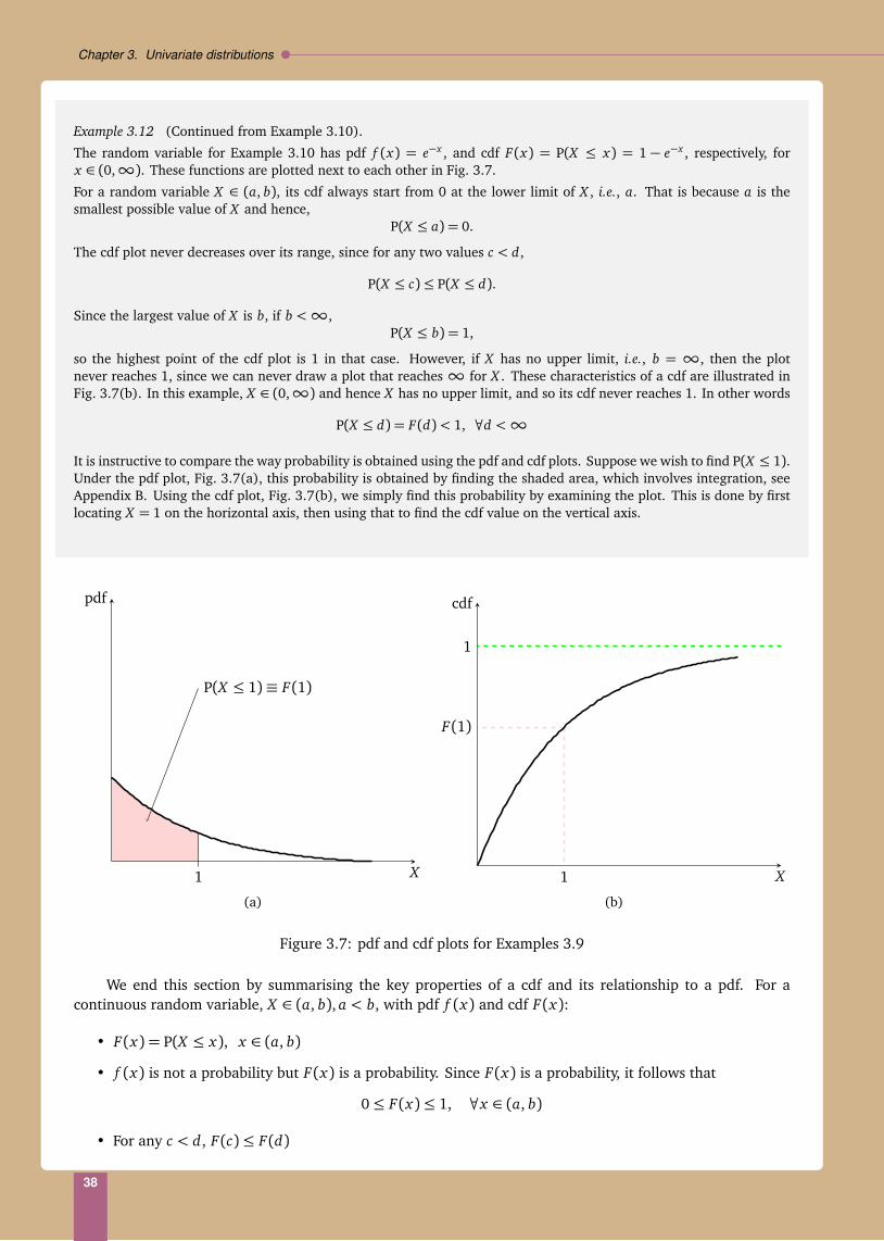
Chapter 3. Univariate distributions
Example 3.12 (Continued from Example 3.10).
The random variable for Example 3.10 has pdf f (x) = e−x , and cdf F(x) = P(X ≤ x) = 1 − e−x , respectively, forx ∈ (0,∞). These functions are plotted next to each other in Fig. 3.7.
For a random variable X ∈ (a, b), its cdf always start from 0 at the lower limit of X , i.e., a. That is because a is thesmallest possible value of X and hence,
P(X ≤ a) = 0.
The cdf plot never decreases over its range, since for any two values c < d,
P(X ≤ c)≤ P(X ≤ d).
Since the largest value of X is b, if b <∞,P(X ≤ b) = 1,
so the highest point of the cdf plot is 1 in that case. However, if X has no upper limit, i.e., b = ∞, then the plotnever reaches 1, since we can never draw a plot that reaches∞ for X . These characteristics of a cdf are illustrated inFig. 3.7(b). In this example, X ∈ (0,∞) and hence X has no upper limit, and so its cdf never reaches 1. In other words
P(X ≤ d) = F(d)< 1, ∀d <∞
It is instructive to compare the way probability is obtained using the pdf and cdf plots. Suppose we wish to find P(X ≤ 1).Under the pdf plot, Fig. 3.7(a), this probability is obtained by finding the shaded area, which involves integration, seeAppendix B. Using the cdf plot, Fig. 3.7(b), we simply find this probability by examining the plot. This is done by firstlocating X = 1 on the horizontal axis, then using that to find the cdf value on the vertical axis.
1
P(X ≤ 1)≡ F(1)
X
(a)
1
F(1)
1 X
cdf
(b)
Figure 3.7: pdf and cdf plots for Examples 3.9
We end this section by summarising the key properties of a cdf and its relationship to a pdf. For acontinuous random variable, X ∈ (a, b), a < b, with pdf f (x) and cdf F(x):
• F(x) = P(X ≤ x), x ∈ (a, b)
• f (x) is not a probability but F(x) is a probability. Since F(x) is a probability, it follows that
0≤ F(x)≤ 1, ∀x ∈ (a, b)
• For any c < d, F(c)≤ F(d)
38

3.3. Continuous distributions
• The following relationships hold between a pdf and its cdf:
F(x) =
∫ x
−∞f (x)d x , f (x) =
dd x
F(x) = F ′(x)
3.3.4 A model for a continuous random variable
At the beginning of Chapter 3.3, we considered finding a model for the hourly wage rate data fromExample 1.13 of Chapter 1. We now return to that problem using the concepts we learned in Chapter 3.3.1-3.3.3. We continue to use X to represent the random variable of interest, so we have 423 observations of X ,and we let X ∈ (0, b), where b is the upper limit of the hourly wage rate, for the population of women. So bis not merely the maximum of the hourly wage rates in the 423 women. We wish to find a probability model(distribution) that describes the data in our sample of women, as well as the population these women belong.Since a probability distribution for a continuous random variable is represented by its pdf, we wish to find anappropriate pdf.
To motivate discussion, we redraw the histogram of the data from Fig. 1.3, except, we divide thefrequencies in each interval of the histogram by n = 423, to give the sample proportion in each interval.The new histogram is given in Fig. 3.8(a). Comparing Fig. 3.8(a) to Fig. 1.3, we notice the histograms areidentical in shape, except the labels on the vertical axis of Fig. 3.8(a) read proportions.
Recall from Chapter 2.2 that probabilities are population proportions and a probability model(distribution) records all the probabilities. Hence a good candidate model is one with pdf that looks likethe sample proportions observed in Fig. 3.8(a); we give an example in Fig. 3.8(b). Our proposed model doesnot need to be exactly the same as the histogram, because our model represents the entire population whereasthe histogram represents the sample, and probability theory allows random variations between observations(hourly wage rates between women) and also between a sample and its population.
Figure 3.8: Histogram of data in Example 1.13 and a proposed model
(a)
Wage
Pro
port
ion
0 5 10 15 20 25 30
00.
10.
20.
3
(b)
Wage
Den
sity
0
0 5 10 15 20 25
To calculate probabilities for a continuous random variable, we need to find the areas under its pdf, whichoften requires integration, see Examples 3.8 - 3.10. Hence, it is useful to find a candidate model such thatintegration under its pdf is easy to carried out, with the condition that it explains the data well. These ideasare illustrated in Example 3.13.
39

Chapter 3. Univariate distributions
Example 3.13
Our pdf for hourly wage rates in Fig. 3.8(b) is drawn using the following function:
f (x) =
¨ x4
e−x/2, 0< x
0, otherwise.
Using this pdf, we can easily find probabilities by integration. In particular, we can find its cdf, F(x), as follows:
F(x) = P(X ≤ x) =
∫ x
0
f (x)d x
=
∫ x
0
x4
e−x/2d x .
Using integration by parts, see Appendix B:∫
udvd x
d x = uv −∫
vdud x
d x . We let u=x2
, sodud x=
12
;dvd x=
12
e−x/2, so v = −e−x/2.
∫ x
0
x4
e−x/2d x =h
−x2
e−x/2ix
0+
∫ x
0
12
e−x/2d x
=h
−x2
e−x/2ix
0+
−e−x/2x
0
=
−(x/2+ 1)e−x/2x
0
= −(x/2+ 1)e−1/2 − (−1)= 1− (x/2+ 1)e−x/2, 0< x .
In 1975, minimum wage in the United States was $2.10. Based on our model, we can use the cdf to estimate theproportion of white working married women below minimum wage in 1975, as follows,
P(X < 2.10) = P(X ≤ 2.1) = F(2.1)= 1− (2.1/2+ 1)e−2.1/2
≈ 0.28.
Hence, according to our model, approximately 28% of the working white married women in the population had hourlywage rate below minimum wage.
Furthermore, according to the US Bureau of Labor Statistics, the average hourly wage in 1975 was $4.53. The proportionof working white married women with hourly wage rate above $4.53 is given by
P(X > 4.53) = 1− P(X ≤ 4.53)= 1− F(4.53)= 1−
1− (4.53/2+ 1)e−4.53/2
≈ 0.34.
Our model tells us only about 34% of the working white married women had hourly wage rate above average hourlywage.
40

4Multivariate Distributions
In Chapter 1, when we introduced the women’s wage data of Example 1.13, in addition to each woman’shourly wage rate, there were seven variables containing information on other socio-economic data of thewomen. These data provide valuable information for understanding these women’s decision to work and ifthey did, their wage dynamics. For example, using all n = 753 women in the dataset, we find 428 womenwere in the workforce in 1975 while 325 women were not. Similarly, among these 753 women, 606 of themdid not have any kids < 6 years, while 118 had one, 26 had two, and 3 women had three kids < 6 years.Using these data, we might be interested in the following question: “Was a woman’s decision to work relatedto the number of kids < 6 years she had?" In this question, we are interested in the two random variables:X=“Workforce status" and Y=“# kids < 6 yrs". To answer such a question, we need to study both randomvariables together. This type of analysis, where we examine the relationship between two or more randomvariables, is called a multivariate analysis (“Multi" = more than one, “variate" = variable). In the currentquestion, there are two random variables, so the analysis is called a bivariate analysis (“Bi" = two, “variate"= variable). A bivariate analysis is an example of a multivariate analysis.
To carry out our bivariate analysis, we first need a way to summarise the data, as we discussed inChapter 1, so we have an impression of what kind of relationship, if there is, holds between X and Y andtherefore, what type of analysis follows. To do this, we summarise our data on X and Y in a contingencytable of frequencies, as follows:
Table 4.1: Contingency table of women classified by workforce status and # kids < 6 years in Example 1.13
X Y (# kids < 6 yrs)(Workforce status) 0 1 2 3 Total
0 (No) 231 72 19 3 3251 (Yes) 375 46 7 0 428Total 606 118 26 3 753
Table 4.1 consists of eight “cells" and two “margins". The number of cells come from the number ofcombinations of categories when women are classified by the two variables X and Y . Since X has two possiblevalues (0 or 1) and Y has four possible values (0, 1, 2 or 3), the total number of possible categories of women,classified by workforce status and # kids < 6 years, is 2× 4 = 8. The two margins give the total number ofwomen for each value of X and Y .
Using Table 4.1, we find that 375 women in the workforce had no kids < 6 years; furthermore, all threewomen who had three kids < 6 years did not work. We can also determine, for example, the 325 women whowere not in the workforce came from four types: 231 with no kids < 6 years, 73 with one kid < 6 years, 19
41
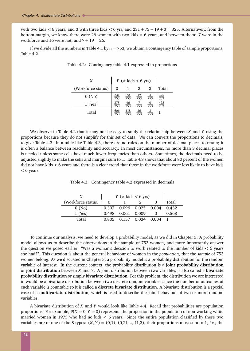
Chapter 4. Multivariate Distributions
with two kids < 6 years, and 3 with three kids < 6 yrs, and 231+ 73+ 19+ 3 = 325. Alternatively, from thebottom margin, we know there were 26 women with two kids < 6 years, and between them: 7 were in theworkforce and 16 were not, and 7+ 19= 26.
If we divide all the numbers in Table 4.1 by n= 753, we obtain a contingency table of sample proportions,Table 4.2.
Table 4.2: Contingency table 4.1 expressed in proportions
X Y (# kids < 6 yrs)
(Workforce status) 0 1 2 3 Total
0 (No) 231753
72753
19753
3753
325753
1 (Yes) 375753
46753
7753
0753
428753
Total 606753
118753
26753
3753 1
We observe in Table 4.2 that it may not be easy to study the relationship between X and Y using theproportions because they do not simplify for this set of data. We can convert the proportions to decimals,to give Table 4.3. In a table like Table 4.3, there are no rules on the number of decimal places to retain; itis often a balance between readability and accuracy. In most circumstances, no more than 3 decimal placesis needed unless some cells have much lower frequencies than others. Sometimes, the decimals need to beadjusted slightly to make the cells and margins sum to 1. Table 4.3 shows that about 80 percent of the womendid not have kids < 6 years and there is a clear trend that those in the workforce were less likely to have kids< 6 years.
Table 4.3: Contingency table 4.2 expressed in decimals
X Y (# kids < 6 yrs)(Workforce status) 0 1 2 3 Total
0 (No) 0.307 0.096 0.025 0.004 0.4321 (Yes) 0.498 0.061 0.009 0 0.568Total 0.805 0.157 0.034 0.004 1
To continue our analysis, we need to develop a probability model, as we did in Chapter 3. A probabilitymodel allows us to describe the observations in the sample of 753 women, and more importantly answerthe question we posed earlier: “Was a woman’s decision to work related to the number of kids < 6 yearsshe had?". This question is about the general behaviour of women in the population, that the sample of 753women belong. As we discussed in Chapter 3, a probability model is a probability distribution for the randomvariable of interest. In the current context, the probability distribution is a joint probability distributionor joint distribution between X and Y . A joint distribution between two variables is also called a bivariateprobability distribution or simply bivariate distribution. For this problem, the distribution we are interestedin would be a bivariate distribution between two discrete random variables since the number of outcomes ofeach variable is countable so it is called a discrete bivariate distribution. A bivariate distribution is a specialcase of a multivariate distribution, which is used to describe the joint behaviour of two or more randomvariables.
A bivariate distribution of X and Y would look like Table 4.4. Recall that probabilities are populationproportions. For example, P(X = 0, Y = 0) represents the proportion in the population of non-working whitemarried women in 1975 who had no kids < 6 years. Since the entire population classified by these twovariables are of one of the 8 types: (X , Y ) = (0,1), (0,2),..., (1,3), their proportions must sum to 1, i.e., the
42

4.1. Discrete bivariate distributions
entire population. This means
P(X = 0, Y = 1)+P(X = 0, Y = 2)+...+P(X = 1, Y = 3) =∑
a
∑
b
P(X = a, Y = b) = 1, a = 0,1, b = 0, 1,2,3.
In Table 4.4, we have deliberately left out the “margins" because we can work them out easily using theprobabilities in the eight “cells" of the table. For example, if we are interested in the population proportion ofwhite married women with no kids < 6 years, we calculate
P(Y = 1) = P(X = 0, Y = 1) + P(X = 1, Y = 1).
This is because women with no kids < 6 years either worked or not worked, and so the two groups add up toall women with no kids < 6 years.
Table 4.4: Joint distribution of workforce status and # kids < 6 yrs in white married women
X Y (# kids < 6 yrs)(Workforce status) 0 1 2 3 Total
0 (No) P(X = 0, Y = 0) P(X = 0, Y = 1) P(X = 0, Y = 2) P(X = 0, Y = 3)1 (Yes) P(X = 1, Y = 0) P(X = 1, Y = 1) P(X = 1, Y = 2) P(X = 1, Y = 3)Total 1
Based on the foregoing discussions, we now formally define a discrete bivariate random variable and itsdistribution, and examine their properties.
4.1 Discrete bivariate distributions
Suppose X and Y are discrete random variables, such that the possible values of X are: a1, a2, ..., ak and thepossible values of Y are b1, ..., bl , where k, l are positive integers ≥ 2. The pair (X , Y ) is called a discretebivariate random variable. A discrete bivariate random variable (X , Y ) is often simply referred to as arandom variable. Some examples of discrete bivariate random variables are given below.
Example 4.1
• Treatment outcome of two patients: X = 1 or 0 for first patient, Y = 1 or 0 for second patient; (X , Y ) =(0,0), (0, 1), (1, 0), (1, 1) (2× 2= 4 possible combinations)
• Outcome of two tosses of a die: X , Y are outcomes for first and second die, respectively, X , Y =1, 2, 3, 4, 5 or 6;(X , Y ) = (1, 1), (1,2), (1,3), ..., (6, 5), (6,6) (6× 6= 36 possible combinations)
• Outcome from tossing one die and one coin: X = outcome for die, Y = outcome for coin, X =1, 2, 3, 4, 5 or 6,Y = H or T ; (X , Y ) = (1, H), (1, T ), (2, H), ..., (6, H), (6, T ) (6× 2= 12 possible combinations)
• No. of infections and no. of recoveries in a large population: X = 0, 1, 2, 3,... are no. of infections (Infinitebut countable no. of possible values) and Y = 0, 1, 2,..., X no. of recoveries out of X infections (∞×∞ =∞possible combinations)
4.1.1 Discrete joint distribution function
A joint probability distribution for a discrete bivariate random variable (X , Y ) links each possible pair of valuesof (X , Y ) to a probability. The probabilities of a joint probability distribution are given by a joint probability
43

Chapter 4. Multivariate Distributions
distribution function (sometimes also called a joint distribution function or simply distribution function ifits is understood that we are referring more than one random variable):
P(X = ai , Y = b j)≡ P(ai , b j), i = 1, ..., k, j = 1, ..., l.
P(X = ai , Y = b j) tells us the proportion of times X = ai and Y = b j occur in the population. A joint probabilitydistribution function is often abbreviated as a joint pdf (or PDF) . A joint pdf has the following properties:
• 0≤ P(ai , b j)≤ 1, ∀ai , b j
•∑
ai
∑
b jP(ai , b j) = 1, i = 1, ..., k, j = 1, ..., l
These properties are similar to those described in Chapter 3.2.2 for a univariate pdf for a discrete randomvariable.
Example 4.2
Let (X , Y ) be a discrete random variable; the possible values for X are 0,1, and for Y are 1, 2, 3, or 4. Furthermore,suppose the distribution of (X , Y ) is given by the following joint pdf:
YX 1 2 3 4 Total0 0.05 0.05 0.1 0.21 0.3 0.15 0.15 0
Total 1
The numbers in the “cells" of the table give the probabilities of occurrence of (X , Y ) = (ai , b j). For example, we findP(X = 0, Y = 1) = P(0, 1) = 0.05, hence (X , Y ) = (0,1) appears 5% of the time.
We can also work out other probabilities, such as the margins. For example,
P(Y = 3) = P(X = 0, Y = 3) + P(X = 1, Y = 3)= 0.1+ 0.15
= 0.25.
The possible values of (X , Y ) are: (0,1), (0, 2), ..., (1,3), (1,4). Hence their proportions must sum to the population:
P(0, 1) + P(0, 2) + ...+ P(1,3) + P(1,4) =∑
ai
∑
b j
P(ai , b j) = 1.
4.1.2 Marginal probability distribution function
Sometimes, we know the joint distribution between two random variables but we might be interested in thebehaviour of one of the variables. For example, in the women’s wage example, we might be interested in theoverall proportion of women with no more than one kid < 6 years, or we may be interested in the proportionof women with no more than 12 years of education. In those cases, we only wish to know the marginalprobability distribution or marginal distribution. A marginal distribution is no more than a univariatedistribution that we discussed in Chapter 3 and therefore, a marginal distribution satisfies all the propertiesof a univariate distribution.
The probabilities of a marginal distribution are given by a marginal probability distribution functionor marginal distribution function (abbreviated as marginal pdf). We have seen examples of marginal pdf’s;they are the margins of Table 4.4. The marginal pdf’s of X and Y , P(X = ai) and P(Y = b j), respectively, canbe calculated using the joint pdf P(X = ai , Y = b j), see Examples 4.3 and 4.4 below.
44

4.1. Discrete bivariate distributions
Example 4.3
Table 4.4 classifies white married women by work force status in 1975 and the number of kids < 6 years. The marginalpdf of Y , number of kids < 6 years, is given in the bottom margin of the table. The probabilities in the marginal pdf are:
P(Y = 0), P(Y = 1), P(Y = 2) and,P(Y = 3).
As mentioned earlier, we can work out these probabilities using the joint pdf; for example:
P(Y = 2) = P(X = 0, Y = 2) + P(X = 1, Y = 2).
Alternatively, the marginal pdf of X , workforce status, is given in the right margin of the table:
P(X = 0) and P(X = 1).
We can also work these out using the joint probabilities in the “cells" of the table, for example,
P(X = 1) = P(X = 1, Y = 0) + P(X = 1, Y = 1) + P(X = 1, Y = 2) + P(X = 1, Y = 3).
From Example 4.3, we deduce that the marginal pdf of X , P(X = ai) can be calculated from P(X = ai , Y = b j),as follows,
P(X = ai) = P(X = ai , Y = b1) + P(X = ai , Y = b2) + ...+ P(X = ai , Y + bl)
=∑
b j
P(X = ai , Y = b j), j = 1, ..., l.
Notice when we calculate the marginal probability of X = ai , we fix X = ai and sum over all possible P(X =ai , Y = b j), for different values of Y . This is because, if we are interested in non-working women, we add upall subsets of non-working women, with 0, 1, 2, or 3 kids < 6 years.
Similarly,
P(Y = b j) =∑
ai
P(X = ai , Y = b j), i = 1, ..., k,
so for example, if we wish to find all women with one kid < 6 years, we add all working women with one kid< 6 years and all non-working women with one kid < 6 years.
Example 4.4 (Continued from Example 4.2)
Y1 2 3 4 Total
X 0 0.05 0.05 0.1 0.2 0.41 0.3 0.15 0.15 0 0.6
Total 0.35 0.2 0.25 0.2 1
Using the joint pdf, we can calculate marginal probabilities such as P(X = 1), as follows:
P(X = 1) = P(X = 1, Y = 1) + P(X = 1, Y = 2) + P(X = 1, Y = 3) + P(X = 1, Y = 4)
=∑
b j
P(X = 1, Y = b j), j = 1, 2,3, 4
= 0.3+ 0.15+ 0.15+ 0
= 0.6.
45
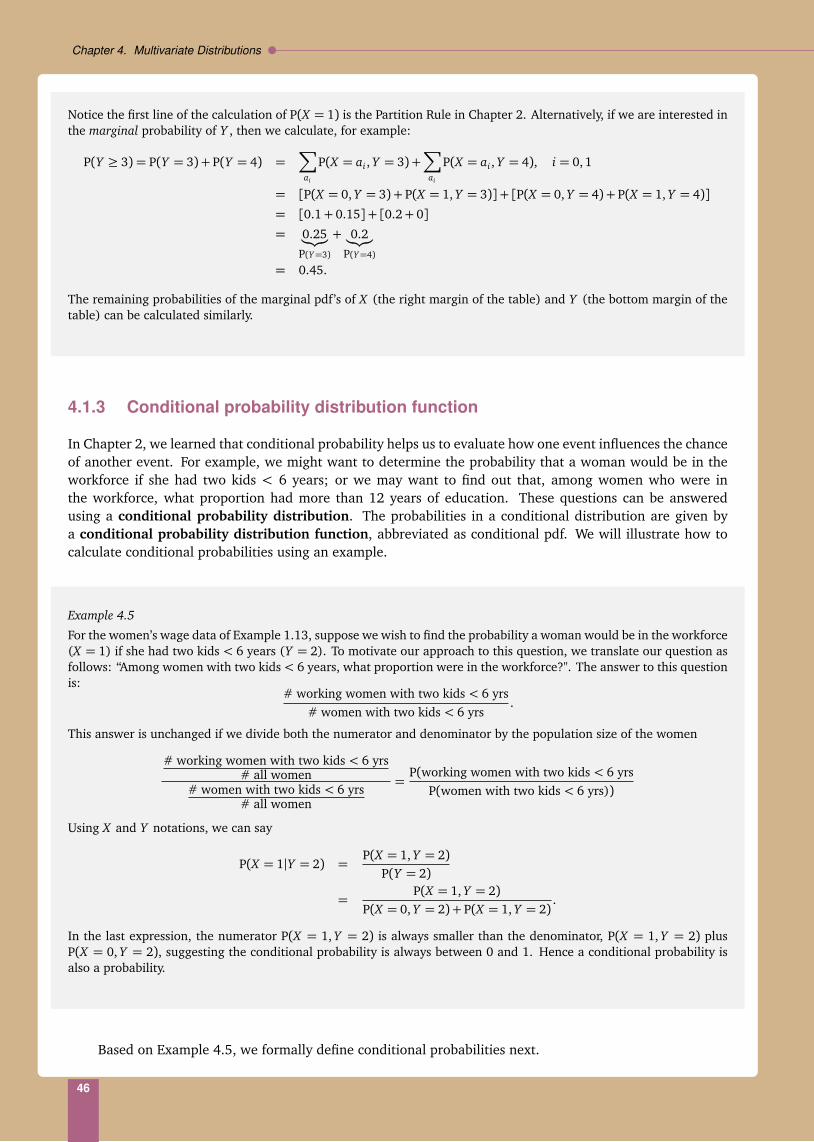
Chapter 4. Multivariate Distributions
Notice the first line of the calculation of P(X = 1) is the Partition Rule in Chapter 2. Alternatively, if we are interested inthe marginal probability of Y , then we calculate, for example:
P(Y ≥ 3) = P(Y = 3) + P(Y = 4) =∑
ai
P(X = ai , Y = 3) +∑
ai
P(X = ai , Y = 4), i = 0, 1
= [P(X = 0, Y = 3) + P(X = 1, Y = 3)] + [P(X = 0, Y = 4) + P(X = 1, Y = 4)]= [0.1+ 0.15] + [0.2+ 0]= 0.25
︸︷︷︸
P(Y=3)
+ 0.2︸︷︷︸
P(Y=4)
= 0.45.
The remaining probabilities of the marginal pdf’s of X (the right margin of the table) and Y (the bottom margin of thetable) can be calculated similarly.
4.1.3 Conditional probability distribution function
In Chapter 2, we learned that conditional probability helps us to evaluate how one event influences the chanceof another event. For example, we might want to determine the probability that a woman would be in theworkforce if she had two kids < 6 years; or we may want to find out that, among women who were inthe workforce, what proportion had more than 12 years of education. These questions can be answeredusing a conditional probability distribution. The probabilities in a conditional distribution are given bya conditional probability distribution function, abbreviated as conditional pdf. We will illustrate how tocalculate conditional probabilities using an example.
Example 4.5
For the women’s wage data of Example 1.13, suppose we wish to find the probability a woman would be in the workforce(X = 1) if she had two kids < 6 years (Y = 2). To motivate our approach to this question, we translate our question asfollows: “Among women with two kids < 6 years, what proportion were in the workforce?". The answer to this questionis:
# working women with two kids < 6 yrs# women with two kids < 6 yrs
.
This answer is unchanged if we divide both the numerator and denominator by the population size of the women
# working women with two kids < 6 yrs# all women
# women with two kids < 6 yrs# all women
=P(working women with two kids < 6 yrs
P(women with two kids < 6 yrs))
Using X and Y notations, we can say
P(X = 1|Y = 2) =P(X = 1, Y = 2)
P(Y = 2)
=P(X = 1, Y = 2)
P(X = 0, Y = 2) + P(X = 1, Y = 2).
In the last expression, the numerator P(X = 1, Y = 2) is always smaller than the denominator, P(X = 1, Y = 2) plusP(X = 0, Y = 2), suggesting the conditional probability is always between 0 and 1. Hence a conditional probability isalso a probability.
Based on Example 4.5, we formally define conditional probabilities next.
46
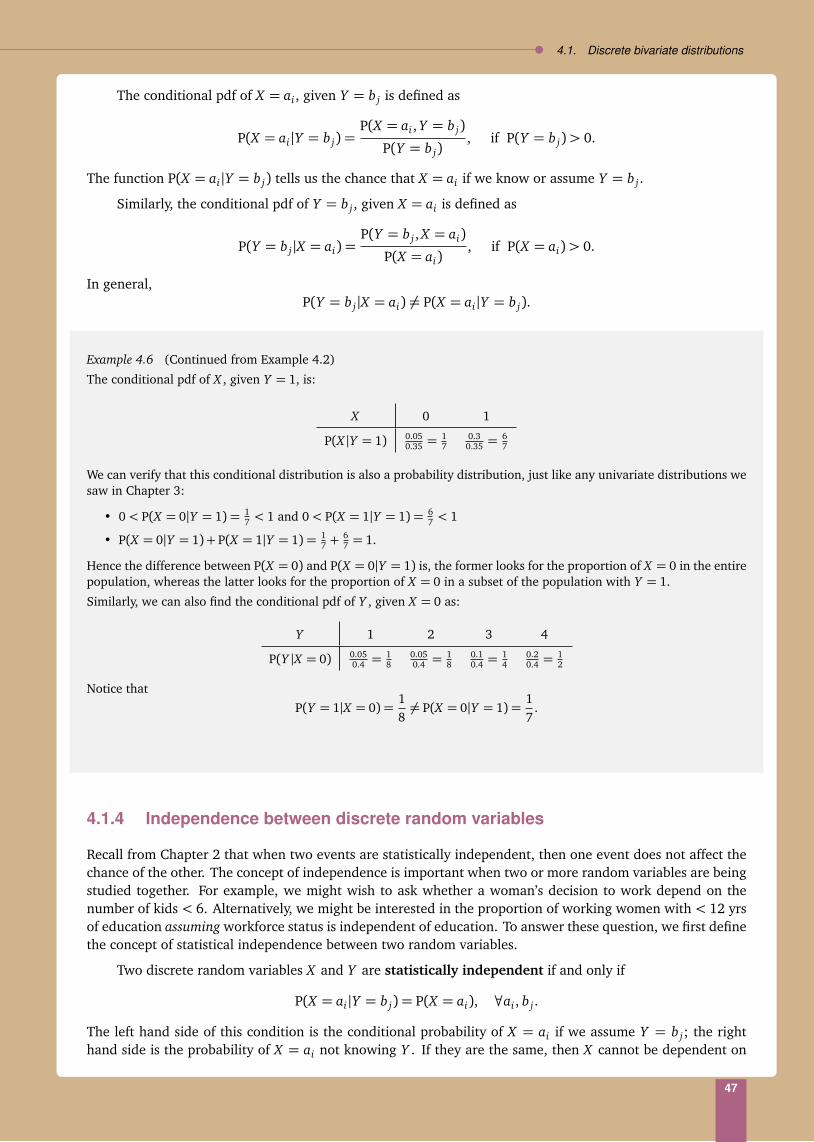
4.1. Discrete bivariate distributions
The conditional pdf of X = ai , given Y = b j is defined as
P(X = ai|Y = b j) =P(X = ai , Y = b j)
P(Y = b j), if P(Y = b j)> 0.
The function P(X = ai|Y = b j) tells us the chance that X = ai if we know or assume Y = b j .
Similarly, the conditional pdf of Y = b j , given X = ai is defined as
P(Y = b j|X = ai) =P(Y = b j , X = ai)
P(X = ai), if P(X = ai)> 0.
In general,P(Y = b j|X = ai) 6= P(X = ai|Y = b j).
Example 4.6 (Continued from Example 4.2)
The conditional pdf of X , given Y = 1, is:
X 0 1
P(X |Y = 1) 0.050.35 =
17
0.30.35 =
67
We can verify that this conditional distribution is also a probability distribution, just like any univariate distributions wesaw in Chapter 3:
• 0< P(X = 0|Y = 1) = 17 < 1 and 0< P(X = 1|Y = 1) = 6
7 < 1
• P(X = 0|Y = 1) + P(X = 1|Y = 1) = 17 +
67 = 1.
Hence the difference between P(X = 0) and P(X = 0|Y = 1) is, the former looks for the proportion of X = 0 in the entirepopulation, whereas the latter looks for the proportion of X = 0 in a subset of the population with Y = 1.
Similarly, we can also find the conditional pdf of Y , given X = 0 as:
Y 1 2 3 4
P(Y |X = 0) 0.050.4 =
18
0.050.4 =
18
0.10.4 =
14
0.20.4 =
12
Notice that
P(Y = 1|X = 0) =186= P(X = 0|Y = 1) =
17
.
4.1.4 Independence between discrete random variables
Recall from Chapter 2 that when two events are statistically independent, then one event does not affect thechance of the other. The concept of independence is important when two or more random variables are beingstudied together. For example, we might wish to ask whether a woman’s decision to work depend on thenumber of kids < 6. Alternatively, we might be interested in the proportion of working women with < 12 yrsof education assuming workforce status is independent of education. To answer these question, we first definethe concept of statistical independence between two random variables.
Two discrete random variables X and Y are statistically independent if and only if
P(X = ai|Y = b j) = P(X = ai), ∀ai , b j .
The left hand side of this condition is the conditional probability of X = ai if we assume Y = b j; the righthand side is the probability of X = ai not knowing Y . If they are the same, then X cannot be dependent on
47

Chapter 4. Multivariate Distributions
Y . The above condition is equivalent to
P(Y = b j|X = ai) = P(Y = b j), ∀ai , b j .
Furthermore, from Chapter 4.1.3, the above implies
P(X = ai|Y = b j) =P(X = ai , Y = b j)
P(Y = b j)= P(X = ai), ∀ai , b j ,
Rearranging gives another equivalence of independence,
P(X = ai , Y = b j) = P(X = ai)P(Y = b j), ∀ai , b j .
Showing one of these three conditions implies independence between X and Y .
Example 4.7 (Continued from Example 4.2)
To find out whether X and Y are independent, we need to use one of the three conditions. For example, we maydetermine whether
P(X = ai , Y = b j) = P(X = ai)P(Y = b j), ∀ai , b j .
Starting with X = 0 and Y = 1, we have
P(X = 0, Y = 1) = 0.05, P(X = 0) = 0.4, P(Y = 1) = 0.35,
SoP(X = 0)P(Y = 1) = 0.4× 0.35= 0.14 6= 0.05= P(X = 0, Y = 1),
therefore, we conclude that X is not statistically independent of Y . Alternatively, we could have shown that
P(X = 0|Y = 4) =P(X = 0, Y = 4)
P(Y = 4)=
0.20.2= 1 6= P(X = 0) = 0.4
to arrive at the same conclusion.
We note that we only need one counter example to show X and Y are not independent, whereas, to demonstrateindependence, we need to prove one of the three conditions, ∀ai , b j , see Example 4.8.
Example 4.8
Suppose X and Y are both discrete random variables with joint pdf:
P(X = ai , Y = b j) =ai b j
18, if ai = 1, 2,3; b j = 1,2.
Their joint pdf is given in the following table.
Y
X 1 2 Total
1 118
218
318
2 218
418
618
3 318
618
918
Total 618
1218 1
48
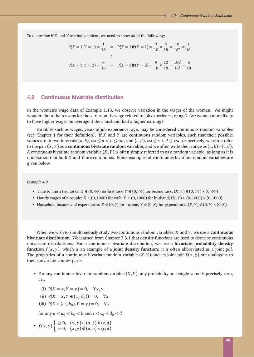
4.2. Continuous bivariate distribution
To determine if X and Y are independent, we need to show all of the following:
P(X = 1, Y = 1) =1
18= P(X = 1)P(Y = 1) =
318×
618=
18182=
118
...
P(X = 3, Y = 2) =6
18= P(X = 3)P(Y = 2) =
918×
1218=
108182
=6
18
4.2 Continuous bivariate distribution
In the women’s wage data of Example 1.13, we observe variation in the wages of the women. We mightwonder about the reasons for the variation. Is wage related to job experience, or age? Are women more likelyto have higher wages on average if their husband had a higher earning?
Variables such as wages, years of job experience, age, may be considered continuous random variables(see Chapter 1 for their definition). If X and Y are continuous random variables, such that their possiblevalues are in two intervals (a, b),∞≤ a < b ≤∞, and (c, d),∞≤ c < d ≤∞, respectively, we often referto the pair (X , Y ) as a continuous bivariate random variable, and we often write their range as (a, b)×(c, d).A continuous bivariate random variable (X , Y ) is often simply referred to as a random variable, as long as it isunderstood that both X and Y are continuous. Some examples of continuous bivariate random variables aregiven below.
Example 4.9
• Time to finish two tasks: X ∈ (0,∞) for first task, Y ∈ (0,∞) for second task; (X , Y ) ∈ (0,∞)× (0,∞)• Hourly wages of a couple: X ∈ (0,1000) for wife, Y ∈ (0, 1000) for husband; (X , Y ) ∈ (0,1000)× (0,1000)
• Household income and expenditure: X ∈ (0, b) for income, Y ∈ (0, X ) for expenditure; (X , Y ) ∈ (0, b)× (0, X )
When we wish to simultaneously study two continuous random variables, X and Y , we use a continuousbivariate distribution. We learned from Chapter 3.3.1 that density functions are used to describe continuousunivariate distributions. For a continuous bivariate distribution, we use a bivariate probability densityfunction f (x , y), which is an example of a joint density function; it is often abbreviated as a joint pdf.The properties of a continuous bivariate random variable (X , Y ) and its joint pdf f (x , y) are analogous totheir univariate counterparts:
• For any continuous bivariate random variable (X , Y ), any probability at a single value is precisely zero,i.e.,
(i) P(X = x , Y = y) = 0, ∀x , y
(ii) P(X = x , Y ∈ (c0, d0)) = 0, ∀x
(iii) P(X ∈ (a0, b0), Y = y) = 0, ∀y
for any a < a0 < b0 < b and c < c0 < d0 < d
• f (x , y)
≥ 0, (x , y) ∈ (a, b)× (c, d)= 0, (x , y) /∈ (a, b)× (c, d)
49

Chapter 4. Multivariate Distributions
• Since f (x , y) is non-negative but P(X = x , Y = y) = 0,∀(x , y) ∈ (a, b) × (c, d), therefore, f (x , y)cannot be interpreted as P(X = x , Y = y). In fact, f (x , y) is not a probability.
• PX ∈ (a0, b0), Y ∈ (c0, d0) is evaluated using “double" integration (see Appendix B),
P(a0 ≤ X ≤ b0, c0 ≤ Y ≤ d0) =
∫ d0
c0
∫ b0
a0
f (x , y)d xd y =
∫ b0
a0
∫ d0
c0
f (x , y)d yd x .
The above identity shows that the order of integration is interchangeable.
• Since (X , Y ) must lie within (a, b)× (c, d), the total “volume" under f (x , y) or probability must be 1:
∫ b
a
∫ d
cf (x , y)d yd x = 1
Suppose we wish to examine the relationship between the wages of a woman (X ) and her husband(Y ). We first summarise the data using histograms, see Fig. 4.1. Fig. 4.1 consists of three histograms. Thetop histogram describes the wages of the 423 working women; this histogram reproduces Figure 1.3. Thehistogram on the right hand margin summarises the wages of the husbands of the 423 women. The finalhistogram, summarises the women’s and their husband’s wages when they are considered simultaneously. Inthis histogram, each bin or bar is an interval defined by (x , x + d x) and (y, y + d y) and the bar above the binrepresents the frequency (or proportion) of (X , Y ) pairs that fall within the interval.
Figure 4.1: Histograms of the wages in 423 women and their spouses in Example 1.13
WageHusb
and's wage
proportion
Wage
Husband's wage
To continue, we need to find a probability model (distribution) that describes the data in our sample ofwomen and their husband’s wage, as well as the population these data belong. Since a probability distributionfor a continuous random variable (X , Y ) is represented by its joint pdf, we wish to find an appropriate jointpdf. Similar to Chapter 3.3.4, we seek a model with pdf that looks like the histogram observed in Fig. 4.1; weshow one such model in Fig. 4.2. As discussed in Chapter 3.3.4, our model does not need to reproduce thehistogram exactly, because the model represents the entire population whereas the histogram represents thesample, and probability theory allows random variations between a sample and its population.
Before we show how to carry out calculations using our probability model, we define a bivariatecumulative distribution function (cdf) by
F(x , y) = P(X ≤ x , Y ≤ y) =
∫ y
c
∫ x
af (x , y)d xd y =
∫ x
a
∫ y
cf (x , y)d yd x .
50

4.2. Continuous bivariate distribution
Figure 4.2: A bivariate model of the women and their husband’s wage for the data in Example 1.13
Wage
Husband's wage
density
Similar to its univariate counterpart (see, Chapter 3.3.3), the bivariate cdf is used for ease of probabilitycalculations involving a random variable (X , Y ). The following relationship also holds between a cdf F(x , y)and its pdf, f (x , y):
f (x , y) =d
d xd
d yF(x , y) =
dd y
dd x
F(x , y).
We now illustrate probability calculations using the model in Fig. 4.2.
Example 4.10We mentioned earlier in Example 3.13 that the criteria for a good model are: (1) a good description of the data and(2) easy probability calculations under the model. We used these criteria to arrive at the joint pdf in Fig. 4.2, which isdrawn using the following function:
f (x , y) =
¨ x
4e−x/2
y4
e−y/2
, 0< x , y
0, otherwise.
Using this pdf, we can easily find probabilities by integration. In particular, we can find its joint cdf, F(x , y), as follows:
F(x , y) = P(X ≤ x , Y ≤ y) =
∫ x
0
∫ y
0
f (x , y)d yd x
=
∫ x
0
∫ y
0
x4
e−x/2 y
4e−y/2
d yd x
=
∫ x
0
x4
e−x/2
d x
∫ y
0
y4
e−y/2
d y
= [
1− (x/2+ 1)e−x/2
︸ ︷︷ ︸
From Example 3.13
1− (y/2+ 1)e−y/2
, 0< x , y.
With the cdf, we can carry out calculations on X , Y , such as:
• P(X ≤ 3, Y ≤ 4) = F(3,4)
=
1− (3/2+ 1)e−3/2
1− (4/2+ 1)e−4/2
≈ 0.263
• P(2< X < 4, Y ≤ 4) = P(X < 4, Y ≤ 4)− P(X < 2, Y ≤ 4)= F(4,4)− F(2, 4)
=
1− (4/2+ 1)e−4/2
1− (4/2+ 1)e−4/2
−
1− (2/2+ 1)e−2/2
1− (4/2+ 1)e−4/2
≈ 0.196
51

Chapter 4. Multivariate Distributions
• P(X > 4, Y ≤ 4) = P(X <∞, Y ≤ 4)− P(X ≤ 4, Y ≤ 4)= F(∞, 4)− F(4, 4)
=
1− (∞/2+ 1)e−∞/2
︸ ︷︷ ︸
=1
1− (4/2+ 1)e−4/2
−
1− (4/2+ 1)e−4/2
1− (4/2+ 1)e−4/2
≈ 0.241.
4.2.1 Marginal probability
Sometimes, we have a joint probability model (distribution) on X and Y , but we might wish to calculateprobabilities on either X or Y only. For example, suppose we have a joint probability distribution on thewages of women and their husbands, but we wish to find out the proportion of men who earned between5-10 dollars an hour. In that case, we need to calculate the marginal probability. There are two ways to findmarginal probabilities from a joint distribution, we illustrate them using the following examples.
Example 4.11 (Continued from Example 4.10)
The proportion of men who earned between 5-10 dollars an hour is defined as
PY ∈ (5,10).
Notice that we are interested in “all men who earned 5-10, irrespective of what their wife earned". Hence the aboveexpression can be re-written as follows:
PY ∈ (5, 10) ≡ PX = any value, Y ∈ (5, 10)≡ PX ∈ (a, b), Y ∈ (5,10)
=
∫ 10
5
∫ b
a
f (x , y)d x︸ ︷︷ ︸
= f (y)
d y
=
∫ 10
5
f (y)d y.
In the above expression,
f (y) =
∫ b
a
f (x , y)d x
is called the marginal probability density function (pdf) of Y . The marginal pdf f (y) is just like the univariate pdf’sin Chapter 3.3. Recall we do not care about the women’s wage, hence the marginal pdf f (y) is obtained from f (x , y)by taking all values of X , i.e.,
∫ b
a f (x , y)d x .
Returning to our calculation, we obtain:
f (y) =
∫ ∞
0
x4
e−x/2 y
4e−y/2
d x
= y
4e−y/2
∫ ∞
0
x4
e−x/2
d x︸ ︷︷ ︸
=F(∞)−F(0)=1 from Example 3.13
= y
4e−y/2
,
52

4.2. Continuous bivariate distribution
from which we have:
P(Y ∈ (5,10)) =
∫ 10
5
f (y)d y
=
∫ 10
5
y4
e−y/2d y
=
−(y/2+ 1)e−y/210
5︸ ︷︷ ︸
From Example 3.13
=
−(10/2+ 1)e−10/2
−
−(5/2+ 1)e−5/2
≈ 0.247.
Example 4.12 (Continued from Example 4.11)
As we observed in Example 4.11, calculating probabilities can become quite tedious. We encountered a similar problemwhen we were dealing with univariate distributions, see Chapter 3.3.3. In Chapter 3.3.3, we explained that a cumulativedistribution function, when available, can be used to expedite calculations. We will use the same strategy here. Supposethe joint cdf of (X , Y ) is F(x , y). Then the marginal cumulative distribution function (cdf) of Y , can be easily obtainedfrom F(x , y) by
F(y) = P(Y ≤ y) = F(∞, y), ∀y.
The expression above can be justified as follows
F(y) ≡ P(Y ≤ y)= P(don’t care about X , Y ≤ y)= P(∀X , Y ≤ y)= P(X ≤∞, Y ≤ y)≡ F(∞, y).
Similarly, we can define F(x) = F(x ,∞).From Example 4.10, we already obtained
F(x , y) = P(X ≤ x , Y ≤ y) = [
1− (x/2+ 1)e−x/2
1− (y/2+ 1)e−y/2
, 0< x , y.
Hence, we can easily find:
F(y) = F(∞, y) = [
1− (∞/2+ 1)e−∞/2
1− (y/2+ 1)e−y/2
=
1− (y/2+ 1)e−y/2
, ∀0< y.
Now
P(5≤ Y ≤ 10) = P(Y ≤ 10)− P(Y ≤ 5)= F(10)− F(5)=
1− (10/2+ 1)e−10/2
−
1− (5/2+ 1)e−5/2
≈ 0.247,
which gives the same answer as in Example 4.11
We summarise from Examples 4.11 and 4.12 the steps to obtain marginal probability:
1. If we know the joint pdf, f (x , y):
53

Chapter 4. Multivariate Distributions
Step 1: Find the marginal pdf’s f (x) and f (y) from the joint pdf f (x , y) using the method in Example 4.11
Step 2: Find marginal probabilities from f (x) and f (y) using the method in Chapter 3.3
2. Using joint CDF F(x , y):
Step 1: Find the marginal cdf’s F(x) and F(y) from F(x , y) using the method in Example 4.12
Step 2: The marginal cdf’s are just the univariate cdf’s we studied in Chapter 3.3; we can use them to workout probabilities on X and Y , using the same methods as Chapter 3.3.2
4.2.2 Independence
We observe from Examples 4.10-4.12 that the joint pdf of (X , Y ) can be factorised as:
f (x , y) = x
4e−x/2
︸ ︷︷ ︸
g(x)
y4
e−y/2
︸ ︷︷ ︸
h(y)
= g(x)h(y).
We call two continuous random variables X and Y independent if we can factorise their joint pdf into twonon-negative functions, g(x)≥ 0 and h(y)≥ 0. When two random variables X and Y are independent or canbe assumed to be independent, the joint probability model becomes very simple since we only need to rely onthe methods in Chapter 3 for probability calculations. In other words, in this case
P(X ≤ x , Y ≤ y) = P(X ≤ x)P(Y ≤ y)
⇒ F(x , y) = F(x)F(y), ∀x , y.
Furthermore, we showed in Example 4.11 that y4 e−y/2 is the marginal pdf of Y ; we can also show that x
4 e−x/2
is the marginal pdf of X . This implies that when X and Y are independent, their joint pdf can be factorisedinto their marginal pdf’s, i.e.,
f (x , y) = f (x) f (y).
In other words, Figure 4.2 for the joint pdf is a “product" of two marginal pdf’s of Figure 3.8.
Example 4.13
Let f (x , y) =§
2x , 0≤ y, x ≤ 10, otherwise . Are X and Y independent?
We can let g(x) = x and h(y) = 2. Since g(x) = x ≥ 0 for all values of 0 ≤ x ≤ 1 and h(y) = 2 ≥ 0 for all values of0≤ y ≤ 1, and f (x , y) = g(x)h(y) therefore, X and Y are independent.
An alternative choice is to write g(x) = 2x and h(y) = 1 and similar arguments as above can be used to show that Xand Y are independent.
Example 4.14
Given f (x , y) =§
6(x − y), 0≤ y ≤ x ≤ 10, otherwise . Are X and Y independent?
In this example, it is not obvious how to factorise f (x , y) as g(x)h(y) because of the restriction y ≤ x . To determinewhether X and Y are independent, we can find the marginal densities of X and Y ,
f (x) =
∫ x
0
6(x − y)d y = 6
x y −y2
2
x
0
= 6
x2 −x2
2
= 3x2, 0≤ x ≤ 1,
f (y) =
∫ 1
y
6(x − y)d x = 6
x2
2− x y
1
y
= 6
12− y
− 6
y2
2− y2
= 3(1− y)2, 0≤ y ≤ 1.
54

4.2. Continuous bivariate distribution
Since f (x) f (y) = 9x2(1− y)2 6= f (x , y) = 6(x − y), therefore X and Y are not independent.
4.2.3 Conditional probability
One of the main goals of studying two or more random variables simultaneously is to see how they influenceeach other. For example, we might wonder whether women with low earning husbands are themselves lowwage earners. In other words, we may be interested to find conditional probabilities such as P(X ≤ x |Y ≤ y)or P(X ≤ x |Y = y). If X and Y are independent, the answers are simple; because X and Y don’t affect eachother, hence, P(X ≤ x |Y ≤ y) = P(X ≤ x) and P(X ≤ x |Y = y) = P(X ≤ x).
Example 4.15 (Continued from Examples 4.10-4.12)
We assumed independence in our model for the wages of women (X ) and their husbands (Y ), hence
P(X ≤ x |Y ≤ y) =P(X ≤ x , Y ≤ y)
P(Y ≤ y)
=
independence︷ ︸︸ ︷
P(X ≤ x)P(Y ≤ y)P(Y ≤ y)
= P(X ≤ x).
For example, if we are interested in the probability of a woman with hourly wage ≤ 5, given her husband earned nomore than 3, the answer is:
P(X ≤ 5|Y ≤ 3) = P(X ≤ 5)= F(5)= 1− (5/2+ 1)e−5/2
≈ 0.713.
Similarly, if we wish to find the probability of a woman with hourly wage ≤ 5, given her husband earned exactly 3, theanswer is:
P(X ≤ 5|Y = 3) = P(X ≤ 5)≈ 0.713,
which is identical to P(X ≤ 5|Y ≤ 3) because, under independence between X and Y , the information of Y is irrelevantwhen we study X .
In general, X and Y may not be independent. In that case, we need to have different approaches toanswer P(X ≤ x |Y ≤ y) and P(X ≤ x |Y = y). To find P(X ≤ x |Y ≤ y), we use
P(X ≤ x |Y ≤ y) =P(X ≤ x , Y ≤ y)
P(Y ≤ y)
=F(x , y)F(y)
.
To find P(X ≤ x |Y = y), we define a conditional probability density function (pdf), which is written asf (x |y) and is calculated by
f (x |y) =f (x , y)f (y)
, f (y)> 0.
55
Chapter 4. Multivariate Distributions
The conditional pdf is undefined at values of y such that f (y) = 0, which correspond to those values of ywith no chance of being observed. Probabilities under a conditional pdf are calculated using its conditionalcumulative distribution function (cdf), defined as
F(x |y) = P(X ≤ x |Y = y) =
∫ x
−∞f (x |y)d x .
Note that even though P(Y = y) = 0 for any value of y , P(X ≤ x |Y = y) is defined. This is because inP(X ≤ x |Y = y) we are not calculating P(Y = y); rather we wish to find the probability about X ≤ x assumingY = y . We can similarly define P(Y ≤ y|X = x).
Example 4.16 (Continued from Example 4.14)
The conditional density of Y given X = x is
f (y|x) =f (x , y)f (x)
=6(x − y)
3x2, 0≤ y ≤ x ≤ 1.
We can find the conditional probability of Y ≤ 14 given X = 1
3 which is
P
Y ≤14|X =
13
=
∫14
−∞
6( 13 − y)
3
13
2 d y
=
∫14
0
6( 13 − y)
3
13
2 d y
= 18
∫14
0
13− y
d y
= 18
13
y −12
y2
14
0
=1812−
1832
=1516
.
56

5Expectation, Variance and Covariance
In Chapter 1, we learned the sample mean and sample variance are useful summaries for a sample ofobservations. In this chapter, we will examine these concepts for a population.
5.1 Expectation and variance of a discrete random variable
In Example 2.1, we obtained data on 9 tosses of a coin:
H T H T T H T H TSuppose we use X to denote the outcome of each toss, such that X = 1 if H is observed and X = 0 otherwise.Then our sample consists of n= 9 observations of X :
(X1, ...Xn) = (1,0, 1,0, 0,1, 0,1, 0).
We can summarise the data using the sample mean:
X =1n
n∑
i=1
X i =1+ 0+ 1+ 0+ 0+ 1+ 0+ 1+ 0
9=
49
.
Another way of expressing the sample mean is:
X =
four 1’s︷ ︸︸ ︷
1+ 1+ 1+ 1+five 0’s
︷ ︸︸ ︷
0+ 0+ 0+ 0+ 09
= 1×49+ 0×
59
,
which can be interpreted as:
sample mean= 1× (sample proportion of 1’s)+ 0× (sample proportion of 0’s).
We apply the idea of calculating a sample mean to find a population mean. In the context of tossing acoin. The population refers to the situation if we had the opportunity to toss the coin many times, then allthe outcomes form the population of outcomes. For a fair coin, we observed in Chapter 3 the distribution ofoutcomes is
Outcome Probability1 (H) 1/20 (T) 1/2
57

Chapter 5. Expectation, Variance and Covariance
Probabilities are population proportions, see Chapter 2.2. Using the idea from calculating a sample mean, wefind
population mean = 1× (population proportion of 1’s)+ 0× (population proportion of 0’s)
= 1
12
+ 0
12
=12
.
The population mean is the average value of X (toss outcome) if it could be observed over and over again.We call this average, the expected value, the expectation, or the mean, and we write it as E(X ) or µX (orsimply µ when there is no risk of confusion)
In general, for a random variable X with possible values a1, a2, ..., ak,
E(X ) = a1P(X = a1) + a2P(X = a2) + ...+ akP(X = ak) =∑
ai
aiP(X = ai).
Example 5.1
In a particular population, the number of cars (X ) in a household has the following distribution:
X 0 1 2 3P(X ) 0.2 0.4 0.3 0.1
Based on the distribution, we know the (population) proportion of households with no cars is 0.2 or 20%, with one caris 0.4 or 40%, etc.. The mean number of cars in a household in this population is:
E(X ) = 0× P(X = 0) + 1× P(X = 1) + 2× P(X = 2) + 3× P(X = 3)= 0× 0.2+ 1× 0.4+ 2× 0.3+ 3× 0.1
= 1.3.
This example shows that even though the number of cars in a household is always an integer, the expected value doesnot need to be an integer. The expectation is just the average number of cars per household.
In Chapter 1, we learned that the sample variance is another useful summary for a set of data. In thecoin toss data, we can calculate the sample variancea of the outcomes as follows
s2 =
∑ni=1(X i − X )2
n
=
1−49
2
+
0−49
2
+
1−49
2
+ ...+
0−49
2
9
=
4 times︷ ︸︸ ︷
1−49
2
+
5 times︷ ︸︸ ︷
0−49
2
9
=
1−49
2 49+
0−49
2 59
.
The sample variance is a measure of the spread of the data. If the sample variance is zero, all the observationsin the sample are identical. Otherwise, it measures the average difference between the observations to their
aIn Chapter 1, we introduced two formulae for the sample variance:∑n
i=1(X i−X )2
n and∑n
i=1(X i−X )2
n−1 . Here we use the version thatdivides by n to give a clearer comparison between the forms of a sample and a population variance
58

5.1. Expectation and variance of a discrete random variable
average. In this data set, 4/9 of the outcomes are 1 (H), each of them differs from the mean by (1− 49)
2; theremaining 5/9 of the outcomes are 0 (T) and each differs from the mean by (0− 4
9)2.
If the coin were tossed many more times, we would like to find the spread of the population of tossoutcomes. Using the idea of calculating the sample variance, we can obtain the population variance of thetoss outcomes, as follows,
1−12
2
×12+
0−12
2
×12=
14
.
In general, for a random variable X with possible values a1, a2, ..., ak and population mean µX , its(population) variance is given by
Var(X ) = (a1 −µX )2P(X = a1) + (a2 −µX )
2P(X = a2) + ...+ (ak −µX )2P(X = ak) =
k∑
i=1
(ai −µX )2P(X = ai).
Once again, sample proportions are replaced by population proportions, or probabilities. The variance of arandom variable has similar use and interpretation as the variance in a set of data. It measures the expecteddifferences of the various possible outcomes from the (population) average. Therefore, a random variablewith a large variance is more likely to have outcomes that are different from the expected value than one thathas a small variance.
As a complement to the variance, we define the (population) standard deviation of X as
SD(X ) =Æ
Var(X ).
The standard deviation is sometimes easier to interpret than the variance because the standard deviation is inthe same measurement unit as the expected value.
Example 5.2 (Continued from Example 5.1)
The spread of the number of cars in different households in the population is:
Var(X ) = (0− 1.3)2 × P(X = 0) + (1− 1.3)2 × P(X = 1) + (2− 1.3)2 × P(X = 2) + (3− 1.3)2 × P(X = 3)= (0− 1.3)2 × 0.2+ (1− 1.3)2 × 0.4+ (2− 1.3)2 × 0.3+ (3− 1.3)2 × 0.1
= 0.81.
Example 5.3
Suppose in a second population, the number of cars (Y ) in a household has the following distribution:
Y 0 1 6P(Y ) 0.5 0.4 0.1
Based on the distribution, we know the (population) proportion of households with no cars is 0.5 or 50% and one car is0.4 or 40%; 10% of the households have 6 cars. In this population, we find:
E(Y ) = 0× 0.5+ 1× 0.4+ 6× 0.1
= 1
Var(Y ) = (0− 1)2 × 0.5+ (1− 1)2 × 0.4+ (6− 1)2 × 0.1
= 3.6.
59
Chapter 5. Expectation, Variance and Covariance
Compared to the population in Example 5.1, this population has a lower number of cars per household (1 vs. 1.3).However the variance here is 3.6, much higher than that in Examples 5.1-5.2. The high variance here reflects a largespread of car ownerships in this population; 90% families have 0 or 1 cars, but a small percentage, 10%, have a muchhigher number of 6 cars.
5.2 Transformation of random variables
• We are often interested in transformations of a random variable, X
• Examples of transformations of X are: X + 2, X 2,p
X , 1/X , ...
• In general, a transformation of X can be written as g(X ) where g is a function of X
Example 5.4 (Continued from Example 5.1)
Suppose each car needs a road tax of 500 dollars per year. We continue to use X to denote the number of cars owned bya household. Let T denote the road tax paid by each household; T is a random variable because the value of T dependson X , which is a random variable. We can derive the distribution of T , as follows. For a household with no cars, thetax is 0× 500 = 0. Since 20% of the households have 0 cars, hence 20% of the households pay 0 dollars of tax. For ahousehold with 1 car, the tax is 1×500= 500 and since 40% of the households have 1 car, hence 40% of the householdpay 500 dollars tax. We can similarly derive that 30% of the households pay 1000 dollars tax and 10% pay 1500 dollarstax. The distribution can be summarised in the following table;
X (No. of cars) 0 1 2 3T = 500X (Tax) 500× 0= 0 500× 1= 500 500× 2= 1000 500× 3= 1500
P(T ) 0.2 0.4 0.3 0.1
Therefore, the values of X are transformed from 0, 1, 2, 3 to 0, 500, 1000, 1500 but the probabilities are NOTtransformed. The average amount of road tax a household pays is:
E(T ) = 0(0.2) + 500(0.4) + 1000(0.3) + 1500(0.1) = 650.
The intuition behind Example 5.4 leads to the following result. For a discrete random variable X and letc and d be any real numbers,
E(cX + d) =∑
ai
(cai + d)P(X = ai)
= c∑
ai
ai P(X = ai) + d∑
ai
P(X = ai)
= cE(X ) + d × 1
= cE(X ) + d.
More generally, if g is a function of X , then
Ecg(X ) + d= cEg(X )+ d.
We notice that the variance of X is given by
Var(X ) =∑
ai
(ai −µX )2
︸ ︷︷ ︸
g(ai)
P(X = ai) = E(X −µX )2,
60

5.3. Expectation and variance for a continuous random variable
and so the variance is a type of mean. Using the above results then
Var(X ) = E(X −µX )2
= E(X 2 − 2µX︸︷︷︸
constant
X + µ2X
︸︷︷︸
constant
)
= E(X 2)− 2µX E(X )︸︷︷︸
µX
+µ2X
= E(X 2)−µ2X .
The last expression for Var(X ) is sometimes more convenient for carrying out calculations.
5.3 Expectation and variance for a continuous random variable
In Example 3.13 of Chapter 3, we proposed a distribution for women’s wage. The distribution (pdf or cdf)allows us to find the proportion of women in different wage intervals. Here, we develop the concepts ofexpected value and variance for describing women’s wage. According to Chapter 1, wage is a continuousvariable. The concepts and properties for expectation and variance for a discrete random variable apply to acontinuous random variable.
For a continuous random variable X ∈ (a, b), with probability density function f (x), the expected valueof X is given by
µX = E(X ) =
∫ b
ax f (x)d x ,
the variance of X is given by
Var(X ) = E(X −µX )2
=
∫ b
a(x −µX )
2 f (x)d x .
Following a similar proof as in the discrete case, we can also use the alternate expression
Var(X ) = E(X 2)−µ2X
=
∫ b
ax2 f (x)d x −µ2
X
We illustrate how to calculate expectation and variance of a continuous random variable using twoexamples.
Example 5.5Suppose X is a continuous random variable with the following pdf:
f (x) =§
3x2, 0< x < 10, otherwise .
E(X ) =
∫ 1
0
x(3x2)d x =
∫ 1
0
3x3d x =
3x4
4
1
0
=34
E(X 2) =
∫ 1
0
x2(3x2)d x =
∫ 1
0
3x4d x =
3x5
5
1
0
=35
Var(X ) = E(X 2)−µ2X =
35−
34
2
= 0.0375
61

Chapter 5. Expectation, Variance and Covariance
Example 5.6
We proposed a pdf: f (x) = x4 e−x/2, 0 < x , for women’s hourly wage rate (X ) in Fig. 3.8(b). The expectation of X can
be interpreted as the average wage rate of the population of women, and is given by
E(X ) =
∫ ∞
0
x f (x)d x
=
∫ ∞
0
xx4
e−x/2d x
=
∫ ∞
0
x2
4e−x/2d x .
Similar to Example 3.13, we need integration by parts,∫
u dvd x d x = uv −
∫
v dud x d x , see Appendix B.
Let u=x2
2, so
dud x= x;
dvd x=
12
e−x/2, so v = −e−x/2.
∫ ∞
0
x2
4e−x/2d x =
=0︷ ︸︸ ︷
−x2
2e−x/2
∞
0
+
∫ ∞
0
xe−x/2d x
= 4
∫ ∞
0
x4
e−x/2d x
= 4
∫ ∞
0
f (x)d x︸ ︷︷ ︸
area under pdf =1
= 4.
We made use of the fact the area under any pdf is one to save time from evaluating the integral.
Based on our model, women’s population average hourly wage rate is 4. For comparison, the sample average hourlywage rate in the 423 women is X ≈ 4.17. Recall that the model (population) does not need to exactly reproduce thedata (sample).
Similarly, we can calculate the variance of X , which is a measure of the spread of the hourly wage rate among womenin the population. We may use the following formula, which is more convenient for calculation,
Var(X ) = E(X 2)−µ2X .
Since we have already obtained E(X ) = 4, we only need to calculate E(X 2), which is
E(X 2) =
∫ ∞
0
x2 f (x)d x
=
∫ ∞
0
x2 x4
e−x/2d x
=
∫ ∞
0
x3
4e−x/2d x .
Once again, we need integration by parts:
Let u=x3
2, so
dud x=
3x2
2;
dvd x=
12
e−x/2, so v = −e−x/2.
62
5.4. Mean and variance of combinations of random variables
∫ ∞
0
x3
4e−x/2d x =
=0︷ ︸︸ ︷
−x3
2e−x/2
∞
0
+
∫ ∞
0
3x2
2e−x/2d x
= 6
∫ ∞
0
x2
4e−x/2d x
︸ ︷︷ ︸
=E(X )=4
= 6(4)= 24.
So, based on our proposed model, the variance of the hourly wage rate in the population of women is:
Var(X ) = 24− 42 = 8.
For comparison, the sample variance based on the 423 women is s2 ≈ 10.2.
5.4 Mean and variance of combinations of random variables
Very often, we would be working with combinations of random variables. For example, in the wage data, wemight be interested in the hourly household earning of a couple, X+Y , where X ∈ (a, b) represents a woman’swage and Y ∈ (c, d) her husband’s wage. Here, we study how to calculate expectation and variance in such asituation.
The quantities E(X + Y ) and Var(X + Y ) tell us, respectively, the average and spread of hourly householdearnings of couples in the population. From Chapter 5.3, X + Y may be considered as a particulartransformation of (X , Y ). Hence, the method of Chapter 5.3 can be used to find E(X + Y ) and Var(X + Y ).We prove it for the discrete case. The same results hold for continuous random variables except discreteprobabilities are replaced by densities and summation by integration.
E(X + Y ) =∑
ai
∑
b j
(ai + b j)P(X = ai , Y = b j)
=∑
ai
∑
b j
ai P(X = ai , Y = b j) +∑
ai
∑
b j
b j P(X = ai , Y = b j)
=∑
ai
ai
∑
b j
P(X = ai , Y = b j)
︸ ︷︷ ︸
=P(X=ai)
+∑
b j
b j
∑
ai
P(X = ai , Y = b j)
︸ ︷︷ ︸
=P(Y=b j)
=∑
ai
aiP(X = ai) +∑
bi
b jP(Y = b j)
= E(X ) + E(Y ).
Notice, in the above, we have made use of the partition rule of Chapter 2. Following similar derivations, wecan also show, for any functions g(·), h(·),
Eg(X ) + h(Y ) = Eg(X )+ Eh(Y ).
63

Chapter 5. Expectation, Variance and Covariance
For variance, following Chapter 5.3,
Var(X + Y ) = E
(X + Y )− E(X + Y )2
= E
(X + Y )− [E(X ) + E(Y )]2
= E
(X −µX ) + (Y −µY )2
= E
(X −µX )2 + (Y −µY )
2 + 2(X −µX )(Y −µY )
= E(X −µX )2+ E(Y −µY )
2+ 2E(X −µX )(Y −µY )= Var(X ) + Var(Y ) + 2Cov(X , Y ).
The term Cov(X , Y ) is called the covariance of X and Y . A positive covariance suggests a positive associationbetween X and Y : if the value of X = ai is larger than expected, i.e., (ai−µX > 0), then Y will often be largerthan expected too (b j − µY > 0). Similarly, if X is smaller than expected, then Y will often to smaller thanexpected too. In contrast, if Cov(X , Y ) < 0, then when X is larger than expected, we will often have Y lowerthan expected, and vice versa. This indicates a negative association between X and Y . It is zero when X andY are independent. We will return to more detailed discussion of Cov(X , Y ) in Chapter 11.
Example 5.7 (Continued from Example 4.10 and Example 5.6)
In Example 5.6, we found for women’s wage, E(X ) = 4, Var(X ) = 8. In our model, the marginal pdfs are identical forthe women’s and their husbands’ wage, therefore, their means and variances must also be the same, E(Y ) = E(X ) = 4and Var(Y ) = Var(X ) = 8. From these, we find
E(X + Y ) = E(X ) + E(Y ) = 8.
Var(X + Y ) = Var(X ) + Var(Y ) + 2 Cov(X , Y )︸ ︷︷ ︸
=0
= 8+ 8= 16.
We used the fact that since X , Y are independent, see Chapter 4.2.2, therefore Cov(X , Y ) = 0.
In Chapters 5.1-5.3, we learned that the properties of expectation and variance are identical betweendiscrete and continuous variables. Similarly, our treatment of E(X +Y ) and Var(X +Y ) for continuous variablealso applies to discrete variables, except density functions are replaced by distribution functions. Specifically,if X and Y are discrete variables, E(X + Y ) = E(X ) + E(Y ) and Var(X + Y ) = Var(X ) + Var(Y ) + 2Cov(X , Y ),where Cov(X , Y ) =
∑
ai
∑
b j(ai −µX )(b j −µY )P(X = ai , Y = b j),b and X = a1, ..., ak, Y = b1, ..., bl .
bWe can write
Cov(X , Y ) = E(X −µX )(Y −µY )= Eg(X , Y )
=∑
ai
∑
b j
g(ai , b j)P(X = ai , Y = b j),
where the last two lines are an application of the results in Chapter 5.2 on expectation of a transformed variable g(X ), to the case ofg(X , Y ). Hence
Cov(X , Y ) =∑
ai
∑
b j
(ai b j − b jµX − aiµY +µXµY )P(X = ai , Y = b j)
=∑
ai
∑
b j
ai b j P(X = ai , Y = b j)−µX
∑
ai
∑
b j
b j P(X = ai , Y = b j)
−µY
∑
ai
∑
b j
ai P(X = ai , Y = b j) +µXµY
∑
ai
∑
b j
P(X = ai , Y = b j)
= E(X Y )−µXµY −µYµX +µXµY
= E(X Y )− E(X )E(Y )
64

5.4. Mean and variance of combinations of random variables
Example 5.8
An insurance agent offers two types of product: life insurance and life annuity. Let X be the number of insurance policiessold per month and Y be number of annuity policies sold per month and the joint pdf between X and Y be:
XY 1 2 3 Total1 0.1 0.2 0.3 0.62 0.1 0.3 0 0.4
Total 0.2 0.5 0.3 1
The marginal pdf’s of X and Y are, respectively,
P(X = 1) = 0.2,P(X = 2) = 0.5,P(X = 3) = 0.3,
P(Y = 1) = 0.6, P(Y = 2) = 0.4.
Furthermore, the joint pdf is,
P(X = 1, Y = 1) = 0.1,P(X = 1, Y = 2) = 0.1, ..., P(X = 3, Y = 2) = 0.
Therefore,
E(X ) = 1(0.2) + 2(0.5) + 3(0.3) = 2.1
Var(X ) = E(X 2)− E(X )2
= 12 × P(X = 1) + 22 × P(X = 2) + 32 × P(X = 3)− E(X )2
= 12(0.2) + 22(0.5) + 32(0.3)− 2.12 = 0.49.
E(Y ) = 1(0.6) + 2(0.4) = 1.4
Var(Y ) = 12(0.6) + 22(0.4)− 1.42 = 0.24.
Cov(X , Y ) = E(X Y )− E(X )E(Y )= (1)(1)P(X = 1, Y = 1) + (2)(1)P(X = 2, Y = 1) +(3)(1)P(X = 3, Y = 1) + (1)(2)P(X = 1, Y = 2) +(2)(2)P(X = 2, Y = 2) + (3)(2)P(X = 3, Y = 2)− E(X )E(Y )
= (1)(1)(0.1) + (2)(1)(0.2) + (3)(1)(0.3) +(1)(2)(0.1) + (2)(2)(0.3) + (3)(2)(0)− (2.1)(1.4)
= −0.14
Hence
E(X + Y ) = 2.1+ 1.4
= 3.5
Var(X + Y ) = 0.49+ 0.24− 2(0.14)= 0.45.
65

6Special Distributions
In this chapter, we will study some popular probability models. Two of these probability models are fordiscrete random variables, they are the binomial and Poisson distributions; two others are for continuousrandom variables, they are the exponential and normal distributions. A number of other special distributionsare in Appendix C.
6.1 Bernoulli trials and binomial distribution
In Example 3.3, we considered tossing a fair coin repeatedly. We assumed in each toss, there are two possibleoutcomes (H or T), P(H) = 1/2 and the outcomes of each toss is independent of the outcomes in other tosses.In the example, we were not interested in the actual order of the outcomes. Rather, we were interested in thetotal number of heads in the tosses.
In the pandemic example in Chapter 2, the treatment outcomes of patients form a sequence that looks like1,1,0,0 or 1,0,1,1, etc., where 1 represents “recovered" and 0 “not recovered". We may assume the probabilityof recovery using a particular treatment is p, 0< p < 1 and the outcome in one patient is not affected by anddoes not affect outcomes in the other patients. Similar to outcomes in tossing a coin, a medical worker or apolicy marker would probably be more interested in the total number of patients recovered than in the actualorder of treatment outcomes.
There is commonality in these two examples that allows us to make some generalisations. If we call eachtoss and each time a patient is treated a “trial", the outcome of interest a “success" and the other outcome a“failure", then both examples consist of a series of repeated trials such that:
i. Each trial has only 2 possible outcomes
ii. The probability of success, 0< p < 1 is the same for every trial
iii. The trial outcomes are independent of one another
We often refer to each trial a Bernoulli triala. A sequence of independent Bernoulli trials with a constantsuccess probability form a Bernoulli process or a Bernoulli sequence.
Example 6.1
aAfter James Bernoulli, 1654-1705
66

6.1. Bernoulli trials and binomial distribution
In Example 3.3, we worked out the probability distribution of the total number of H ’s in three tosses. Here, we repeatthe same exercise for the sequence of possible outcomes in 4 patients, assuming the probability of recovery is 0.7 ineach. The possible sequences of outcomes can be enumerated as follows (1= recovered, 0 = not recovered):
1111 (all 4 recovered)
1110, 1101, 1011, 0111 (3 recovered)
1100, 1010, 1001, 0011, 0101, 0110 (2 recovered)
1000, 0100, 0010, 0001 (1 recovered)
0000 (0 recovered)
We can calculate P(4 recovered)= P(1111)= (0.7)(0.7)(0.7)(0.7)= (0.7)4 since each patient has probability of recovery= 0.7 and the outcomes are independent of each other.
Similarly, P(3 recovered)= P(1110) + P(1101) + P(1011) + P(0111). We can calculate P(1110) as (0.7)(0.7)(0.7)(0.3)since the probability of three recovered is 0.7 each and the probability of the last 0 is 1 − P(1) = 0.3. The otherprobabilities are similarly calculated, giving P(3 recovered) = 4(0.7)(0.7)(0.7)(0.3) = 4(0.7)3(1− 0.7).Furthermore, P(2 recovered)= P(1100)+ P(1010)+ P(1001)+ P(0011)+ P(0101)+ P(0110)= 6(0.7)(0.7)(0.3)(0.3)= 6(0.7)2(1− 0.7)2.
P(1 recovered) = 4(0.7)(0.3)(0.3)(0.3) = 4(0.7)(1− 0.7)3.
P(0 recovered) = (0.3)(0.3)(0.3)(0.3) = (1− 0.7)4.
Summarising the results we have the following probability distribution table.b
Table 6.1: Probability distribution for the number of recoveries in 4 patients, each with P(recovery)=0.7
Number of recoveries Probability
0 (0.7)0(1− 0.7)4 = 0.00811 4(0.7)1(1− 0.7)3 = 0.07562 6(0.7)2(1− 0.7)2 = 0.26463 4(0.7)3(1− 0.7)1 = 0.41164 (0.7)4(1− 0.7)0 = 0.2401
From Examples 3.3 and 6.1, we observe that calculating the probability distribution of the total numberof successes can be a tedious task. On the other hand, we observe a pattern emerging from Tables 3.1 and6.1, that we may be able to exploit. This in fact, has been done and the results are record below.
Let X be the number of successes in a sequence of n independent Bernoulli trials each with probability ofsuccess p. The possible values of X are 0, 1, ..., n and hence X is a discrete random variable. The probabilitiesof different values of X form a Binomial distribution with parameters n and p. Sometimes we write X ∼Bin(n, p) for short.
If X ∼ Bin(n, p), the pdf of X is given by the following simple formula,
P(X = k) =
nk
︸︷︷︸
(3)
pk︸︷︷︸
(1)
(1− p)n−k︸ ︷︷ ︸
(2)
, k = 0,1, ..., n
where
nk
=n!
(n− k)!k!
is defined in Appendix B.
Explanation
An outcome with k successes and (n− k) failures has probability equal to (3)× (1)× (2) because
(1) k trials succeed, each with probability p
67

Chapter 6. Special Distributions
(2) (n− k) trials fail, each with probability (1− p)
(3) Furthermore, there aren
k
possible outcomes with k successes and (n− k) failures, see Example 6.1
The parameters n and p are very useful, they allow us to use the Binomial distribution to model differentsituations by changing the values of n and p to suit the context that we are interested in. For example, whenwe are interested in the number of heads, X in three tosses of a coin, then X ∼ Bin(n = 3, p = 0.5) can beused. On the other hand, if X is the number of patients out of 4 who recovered after being given treatment,then X ∼ Bin(n = 4, p = 0.7). Parameters also permit a simple way to describe a particular situation, so forexample, if we are told the number of recoveries from a disease follow a Bin(n= 4, p = 0.7) distribution, wecan picture the situation based on our understanding of the Binomial distribution. Many useful probabilitydistributions (models) also have parameters so they can be used to solve problems in different situations.
Expectation and variance
If X ∼ Bin(n, p) thenE(X ) = npc, Var(X ) = np(1− p),
where E(X ) and Var(X ) are the mean and the variance of X .
Example 6.2
Continuing the pandemic example, suppose we are interested in the total number of recoveries, X , in 10 patients. ThenX ∼ Bin(10, 0.7). (a) What is the probability of seeing 3 in 10 recover? (b) What is the probability of seeing no morethan 3 in 10 recover? (c) What is the expected number of patients out of 10 that recover? (d) What is the variance?
(a)P(X = 3) =
103
(0.7)3(1− 0.7)10−3
≈ 0.009.
So there is very little chance that only 3 out of 10 recover if the probability of recovery is 0.7 each
(b)P(X ≤ 3) =3∑
X=0
10X
(0.7)X (1− 0.7)10−X
=
100
(0.7)0(1− 0.7)10 +
101
(0.7)1(1− 0.7)9 +
102
(0.7)2(1− 0.7)8 +
103
(0.7)3(1− 0.7)7
≈ 0.0106.
(c) The expected number of recoveries in 10 patients is:
E(X ) = np = 10× 0.7= 7
c
E(X ) = 0× P(X = 0) + 1× P(X = 1) + ...+ n× P(X = n)
=n∑
k=1
kP(X = k), 1st term is zero
=n∑
k=1
kn!
k!(n− k)!pk(1− p)n−k
=n∑
k=1
n!(k− 1)!(n− k)!
pk(1− p)n−k
=n∑
k=1
np(n− 1)!
(k− 1)!(n− 1)− (k− 1)!pk−1(1− p)(n−1)−(k−1)
= npm∑
j=0
m!j!m− j!
p j(1− p)m− j
︸ ︷︷ ︸
=1;Bin(m,p)
, let j = k− 1, m= n− 1
= np
We can derive Var(X ) similarly.
68

6.2. Poisson distribution
(d) The variance is:Var(X ) = np(1− p) = 10× 0.7(0.3) = 2.1
The pdf of a random variable can be represented as a table, as in Table 6.1. Alternatively, it can also berepresented as a histogram (Fig. 6.1), see also Chapter 3.2.2. The histogram shows 5 bars, with the area of
Figure 6.1: Histogram showing the pdf of the number of recoveries in 4 patients, each with probability ofrecovery=0.7
0 1 2 3 4
Number of recoveries
Pro
babi
lity
0.0
0.1
0.2
0.3
0.4
each bar equal the probability of observing the value shown at the bottom of each bar. For example, the areaof the bar above “3" is precisely 0.4116. We can also add the areas under different bars. For example, addingthe areas of the bars above “2", “3" and “4" gives the probability of seeing 2 or more recoveries in 4 patients.
Shape
The shape of a Binomial distribution depends upon the values of n and p (Fig 6.2). For small n, thedistribution is almost symmetrical for values of p close to 0.5, but highly skewed for values of p close to 0 or1. As n increases, the distribution becomes more and more symmetrical, for almost all values of p except whenp is very close to 0 or 1. The binomial distribution is always unimodal. A symmetric unimodal distributionis a distribution such that:
1. Mean=median=mode
2. The chance of observing any value a units above the mean (median) is same as the chance of observinga units below the mean (median), i.e., P(mean+a)=P(mean−a) (symmetry).
In a skewed distribution, (1) may still hold but (2) will not.
6.2 Poisson distribution
The Bernoulli process is useful for situations when an event either occurs (success) or does not occur (failure)over a predetermined number of n trials. Sometimes, a type of event does not over a number of defined trials;rather it may occur at any time or at any place. For example, the time of occurrence of the next financial crisis,
69

Chapter 6. Special Distributions
Figure 6.2: pdf’s for Bin(n, p) for various values n and p
0 1 2 3 4 5 6 7 8 9
n=10,p=0.5
X
Pro
babi
lity
0.00
0.05
0.10
0.15
0.20
0 1 2 3 4 5 6 7 8 9
n=10,p=0.9
X
0.0
0.1
0.2
0.3
85 88 91 94 97 100
n=100,p=0.9
X
0.00
0.02
0.04
0.06
0.08
0.10
0.12
or the place of the next accident. In those cases, a Poisson processd may be suitable. The Poisson process canbe considered a continuous-time (or space) analogue of the Bernoulli process. In this section, we will discussthe Poisson process in a time context; its application in a space context is identical and is omitted.
A Poisson process is a model for the occurrence of events, such that
i. No two events occur at the same timeii. The rate of occurrence of events is constant over timeiii. Events occur independently of each other
Just as we were interested in the total number of successes in a Bernoulli process, when we study a Poissonprocess, we often wish to study the total number of events over a particular time interval. The number of eventsover a particular time interval is a discrete random variable. However, unlike the number of successes in aBernoulli process of n trials, which can be 0, 1,..., n−1, n, the possible number of events in a time interval canbe 0, 1, 2, ..., with no upper limit. The probability distribution for the number of events in a Poisson processis called a Poisson distribution.
To motivate discussion of the pdf for a Poisson distribution, we assume that we are interested in thenumber of events, X , over one unit of time interval. Let 0< λ be the rate of occurrence of events over the timeinterval. The pdf consists of probabilities that link each of the possible values of X , i.e., P(X = k), k = 0, 1,2, ....
Imagine splitting the time interval into a large number of n tiny equal intervals, such that in each tinyinterval, either one event or no event occurs, and there is practically no chance two or more events occur.Furthermore, since events occur at a constant rate λ in the time interval, the probability of occurrence ofevents is identical in each tiny interval.
If we view an interval with an event a “success", then occurrence of events at the n tiny intervals is similarto a Bernoulli process, and Y , the number of intervals with an event (successes) over the n tiny intervals hasa Bin(n, p) distribution, where p = λ/n or λ= np. This situation is depicted in Fig. 6.3.
Viewed as Fig. 6.3, we can approximate the pdf of X as follows:
P(X = k) ≈ P(Y = k)
=
nk
pk(1− p)n−k
=
nk
λ
n
k
1−λ
n
n−k
dAfter Siméon-Denis Poisson (1781 - 1840)
70

6.2. Poisson distribution
0 p 1n
p 2n
p 3n
p 4n
p 5n
X , Average number of events = λ
Y , Average number of intervals with an event = np = nλn = λ
n−1n
p 1time
Figure 6.3: Approximating a Poisson process as a Binomal process
=n(n− 1)(n− 1) · · · (n− k+ 1)
k!
λ
n
k
1−λ
n
n−k
=nn·
n− 1n· · ·
n− k+ 1n
︸ ︷︷ ︸
→1
λk
k!
1−λ
n
n
︸ ︷︷ ︸
→e−λ
1−λ
n
−k
︸ ︷︷ ︸
→1
≈λk
k!e−λ, as n→∞
Once the pdf is derived, quantities such as expectation and variance can be obtained similar to those for aBinomial distribution. We summarise below the characteristics of a Poisson distribution.
If X has a Poisson distribution with average rate 0< λ, we write X ∼ Poisson(λ), the pdf of X is
P(X = k) =λk
k!e−λ for k = 0, 1,2, ...
Mean and variance
E(X ) = Var(X ) = λ
Example 6.3
Fig 6.4 records the major financial crises from 1980-2010. We may consider a Poisson process to model the occurrencesof financial crises. Under a Poisson process, we assume the rate of occurrence of crises, 0< λ, is constant over time. Weobserved a sample of 8 crises over 3 decades, so the observed rate of crises is about 8/3≈ 2.67 per decade. Suppose weuse λ = 2.5 (Recall a model is for the population, which does not need to exactly reproduce the sample), then we areeffectively assuming the number of crises in a decade, X , follows a Poisson(2.5) distribution.
We can use our model to find probabilities about X . For example, if we are interested in the chance of 2 crises in thenext decade:
P(X = 2) =2.52
2!e−2.5 ≈ 0.26.
80
Mexican
82
S&L
84
Black Mon.
87
Comm. RE
91
Asian
97
LTCM
98
Dotcom
00
Subprime
07 10
Figure 6.4: Poisson process model for major financial crises 1980-2010
Sum of independent Poisson random variables
71

Chapter 6. Special Distributions
If X and Y are independent, and X ∼ Poisson(λ), Y ∼ Poisson(µ), then
X + Y ∼ Poisson(λ+µ)
Change of time frame
Let X ∼ Poisson(λ) represents the number of events in one unit of time. If we are interested in Y , thenumber of events in t units of time, then Y ∼ Poisson(tλ). This result makes sense since in a Poisson process,the rate of occurrence of events is constant over time, hence a time frame of t units should have a rate that ist times the rate λ for 1 unit of time.
Poisson approximation
The derivation of the pdf of X gives rise to the so-called Poisson approximation to the Binomialdistribution, which says, if Y ∼ Bin(n, p), such that n is large and p is small,e then we can calculateP(Y = k), k = 0, 1, ..., n − 1, n using the pdf of X , if we let λ = np and X ∼ Poisson(λ)f. We illustratethis concept using an example.
Example 6.4
Suppose, everyday, there is a constant probability p = 0.0001 that an earthquake will occur. Then the number of dayswith earthquake, Y , in 10 years is Bin(3650,0.0001). We show that we can calculate P(Y = k) using the binomial pdfor we can approximate the pdf of Y by P(X = k), assuming X ∼ Poisson(λ= np = 0.365).
k
0 1 2 3 4 5
P(Y = k) =n
k
pk(1− p)n−k 0.694184 0.253402 0.046238 0.005623 0.000513 0.000037
P(X = k) = λk
k! e−λ 0.694197 0.253382 0.046242 0.005626 0.000513 0.000037
We observe from the table, that probabilities calculated using the approximate Poisson formula (bottom row of the table)are very similar to the corresponding values using exact formula (top row of the table).
6.3 Exponential distribution
In a Poisson process, events occur over a time interval. There are two main questions we might be interestedin: (1) the number of events in the interval and (2) the time of occurrence of events. In Chapter 6.2, we usedthe Poisson distribution to study (1). Here, we consider (2). Let T denote the time to occurrence of an event(e.g., earthquake, financial crisis). Since T is a time and it is not possible to predict the exact time or how longwe have to wait for the event to occur, we may assume T ∈ (0,∞). Consequently, T is a continuous randomvariable.
The distribution of a continuous random variable is described by its probability density function (pdf) andits cumulative distribution function (cdf). In a Poisson process, events occur over a constant rate, 0 < λ, perunit time. Suppose X t represents the number of events by time t, then from Chapter 6.2, X t ∼ Poisson(λt).
eThere is no general rule as the how large n should be, etc.. As a rough guide, the approximation is good as long as n > 30 andnp < 5 (n(1− p)< 5).
fEven though Y 6= X technically, since X can have values 0, 1, 2,... but Y ’s values are 0, 1, ...,n, but as long as n is large and p istiny, P(X = n+ 1), P(X = n+ 2), .... are practically zero.
72

6.3. Exponential distribution
t
f (t)
λ= 0.5λ= 0.25
00
Figure 6.5: Densities for two exponential distributions
Let T = waiting time to the event. The cdf of T is:
F(t) = P(T ≤ t) = 1− P(T > t)
= 1− P(have to wait longer than time t before the 1st event)
= 1− P(there are no events in time from 0 to t)
= 1− P(X t = 0)
= 1−(λt)0
0!e−λt
= 1− e−λt if t ≥ 0.
Clearly, F(t) = 0 if t < 0. Recall the relationship between the pdf and cdf, such that
f (t) =dF(t)
d t= λe−λt .
The distribution of T is called an exponential distribution. We write T ∼ Ex p(λ), where 0 < λ is theparameter.
In fact, the exponential distribution is not restricted to time to an event, it also applies to any time Tbetween events. In other words, in a Poisson process, the times to the first event and between events all followEx p(λ). We summarise the main characteristics of an exponential distribution below.
pdf and cdf
f (t) =
λe−λt , t > 00, t ≤ 0
F(t) =
1− e−λt , t > 00, t ≤ 0
A graph of the pdf of Ex p(λ) for two different values of λ is given in Fig. 6.5.
Mean and variance
E(T ) =1λ
, Var(T ) =1λ2
Example 6.5 (Continued from Example 6.3)If the number of financial crises, X , in the next decade follows a Poisson(λ= 2.5) distribution, then the time to the nextcrisis, T ∼ Ex p(λ= 2.5). The probability of observing the next crisis in this decade is
P(T ≤ 1)︸ ︷︷ ︸
unit is a decade
= F(1) = 1− e−2.5(1) ≈ 0.92
73

Chapter 6. Special Distributions
and the expected time to the next crisis is
E(T ) =1
2.5= 0.4 decade or 4 years
and the variance is
Var(T ) =1
2.52= 0.16.
The value of the variance helps us assess how likely the actual time to the next crisis would deviate from the average of0.4 decade
Memoryless property
The Exponential distribution is famous for its property of being “memoryless". Suppose T ∼ Ex p(λ) isthe waiting time for an event, and we have already waited time s. What is the chance we have to wait foranother time t? The answer is given by
P(T > s+ t|T > s) =P(T > s+ t, T > s)
P(T > s)
=P(T > s+ t)
P(T > s)
=1− P(T ≤ s+ t)
1− P(T ≤ s)
=1− (1− e−λ(s+t))1− (1− e−λ(s))
=e−λ(s+t)
e−λs
= e−λt
= P(T > t) if t ≥ 0
The expression e−λt , does not depend on s. Therefore, the exponential distribution “forgets" that we havewaited for s — this is called the memoryless property.
Example 6.6 (Continued from Example 6.3)
Suppose T stands for the time between the last and the next crises. What is the chance T > 5 years given it has been 3years since the last crisis? We first convert time into decades; 5 years= 0.5 decades and 3 years = 0.3 decades
P(T > 0.5|T > 0.3) = P(T > 0.2+ 0.3|T > 0.3)= P(T > 0.2)= 1− P(T ≤ 0.2)= 1− (1− e−2.5(0.2))≈ 0.61,
where the last line is due to the fact that the exponential distribution forgets about the wait in the past 0.3 decades, andhence the conditional probability of waiting 0.2 decades beyond 0.3 decades is the same as the unconditional probabilityof waiting 0.2 decades.
74

6.4. Normal distribution
6.4 Normal distribution
One of the most important distributions is called the Normal distribution. The normal distribution issometimes called a Gaussian distribution.g It is a model for continuous random variables. The normaldistribution is important because of two reasons. First, many quantities follow a normal distribution, e.g.,adult height, adult weight and many other biological quantities.h The errors of repeated measurements of afixed entity also often follow a normal distribution.i Second, the normal distribution is central to our abilityto use data in a sample to draw conclusions about unknown quantities in a population, a topic that we willstudy later in this set of notes.
Fig. 6.6 shows a histogram of heights for a sample of individuals. To model heights from this set of data,we have come up with a proposed model. The pdf is superimposed on the histogram.
Figure 6.6: Probability model for heights
Height (cm)
prop
ortio
n
100 150 200 250
0.00
0.01
0.02
0.03
0.04
0.05
0.06
The pdf is in fact that of a normal distribution. The pdf is bell-shaped, hence a normal pdf is sometimescalled a bell-curve. The center of the pdf is the mean of the distribution. The mean of a normal distributionis sometimes denoted by the Greek alphabet µ (pronounced “mu"). In Fig. 6.6, the center of the distributionis at 172 cm and therefore, µ = 172 cm. The mean tells us the average value in the population. A normaldistribution is symmetric about its mean, such that mean = median = mode. Therefore, the median height ofthe population is also 172 cm (i.e., half of the population are taller than 172 cm and half of them are shorterthan 172 cm) and the most likely height in the population is also 172 cm. As seen in Fig. 6.6, the normaldensity is tallest around the mean and the curve drops off symmetrically on either side of the mean. Since thearea under the pdf is higher in the middle than around its tails, the shape of the normal pdf tells us that themost probable values are near the center (the mean) and the probability of seeing values different from themean drops off symmetrically on either side. How quickly the pdf drops off on either side of the mean dependson the standard deviation or equivalently, the variance in the population. In Fig. 6.6, the standard deviation ofthe pdf is 15 cm. We can compare it to another normal pdf with the same mean but with a standard deviationof 7.5 cm (Fig. 6.7).
Compared to Fig. 6.6, the pdf in Fig. 6.7 is narrower and the peak at the center is more pronounced. Anarrower and sharper pdf tells us that, for the population in Fig. 6.7, it is more likely to find people whoseheight are near the mean and less likely to find people who are either very tall or very short. We can understandwhy a small standard deviation leads to a sharper pdf by considering the following. In Chapter 1, we learnedthat the standard deviation (or the variance) measures the average distance of observations in a dataset fromtheir mean. Therefore, a smaller standard deviation tells us the average distance of values from the mean issmaller, which suggests that the probability of seeing values far away from the mean is small, as reflected in a
gAfter Carl Freidrich Gauss, 1777-1855hMany geneticists now believe that many biological quantities follow the normal distribution as a result of polygenic inheritanceiC.F. Gauss is known to be the first person to notice that errors in measurements follow the normal distribution.
75
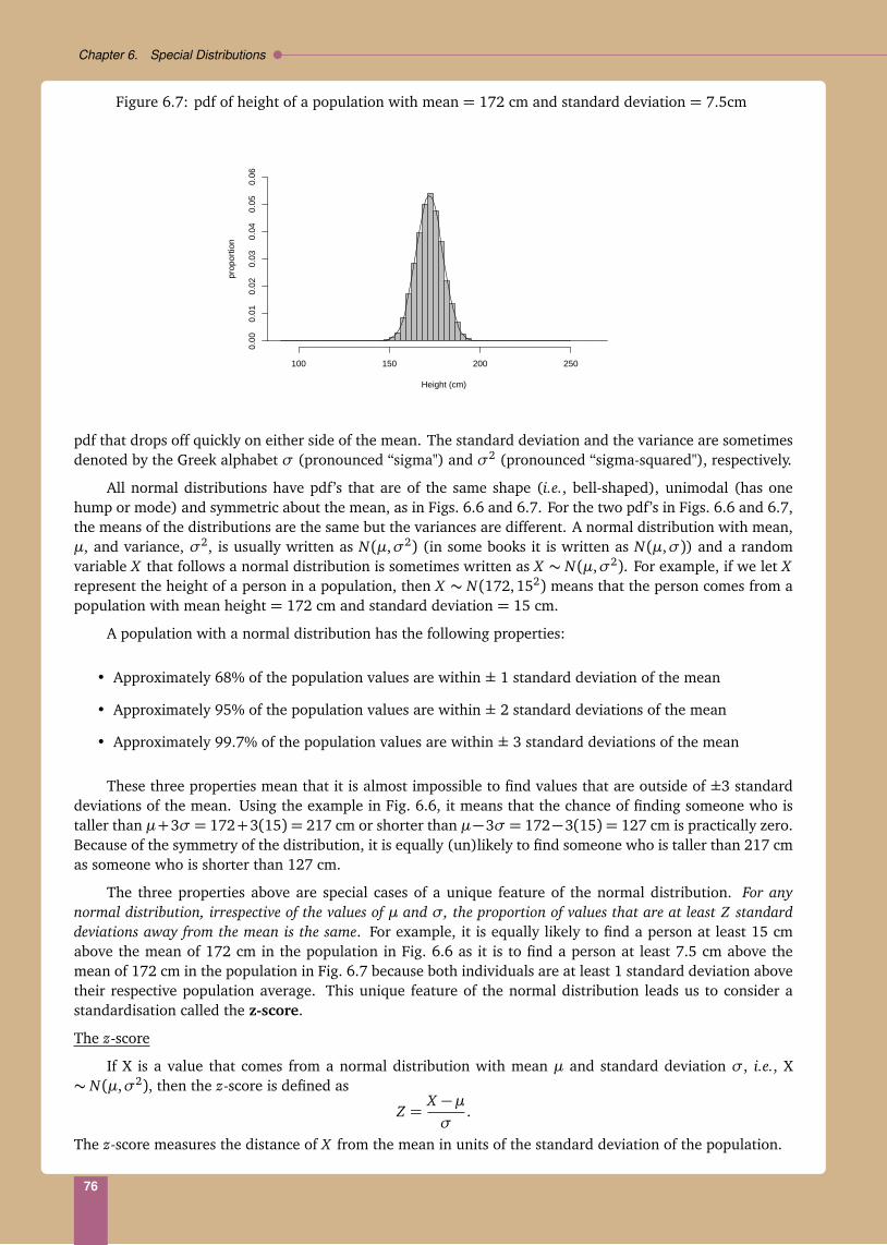
Chapter 6. Special Distributions
Figure 6.7: pdf of height of a population with mean = 172 cm and standard deviation = 7.5cm
Height (cm)
prop
ortio
n
100 150 200 250
0.00
0.01
0.02
0.03
0.04
0.05
0.06
pdf that drops off quickly on either side of the mean. The standard deviation and the variance are sometimesdenoted by the Greek alphabet σ (pronounced “sigma") and σ2 (pronounced “sigma-squared"), respectively.
All normal distributions have pdf’s that are of the same shape (i.e., bell-shaped), unimodal (has onehump or mode) and symmetric about the mean, as in Figs. 6.6 and 6.7. For the two pdf’s in Figs. 6.6 and 6.7,the means of the distributions are the same but the variances are different. A normal distribution with mean,µ, and variance, σ2, is usually written as N(µ,σ2) (in some books it is written as N(µ,σ)) and a randomvariable X that follows a normal distribution is sometimes written as X ∼ N(µ,σ2). For example, if we let Xrepresent the height of a person in a population, then X ∼ N(172,152) means that the person comes from apopulation with mean height = 172 cm and standard deviation = 15 cm.
A population with a normal distribution has the following properties:
• Approximately 68% of the population values are within ± 1 standard deviation of the mean
• Approximately 95% of the population values are within ± 2 standard deviations of the mean
• Approximately 99.7% of the population values are within ± 3 standard deviations of the mean
These three properties mean that it is almost impossible to find values that are outside of ±3 standarddeviations of the mean. Using the example in Fig. 6.6, it means that the chance of finding someone who istaller than µ+3σ = 172+3(15) = 217 cm or shorter than µ−3σ = 172−3(15) = 127 cm is practically zero.Because of the symmetry of the distribution, it is equally (un)likely to find someone who is taller than 217 cmas someone who is shorter than 127 cm.
The three properties above are special cases of a unique feature of the normal distribution. For anynormal distribution, irrespective of the values of µ and σ, the proportion of values that are at least Z standarddeviations away from the mean is the same. For example, it is equally likely to find a person at least 15 cmabove the mean of 172 cm in the population in Fig. 6.6 as it is to find a person at least 7.5 cm above themean of 172 cm in the population in Fig. 6.7 because both individuals are at least 1 standard deviation abovetheir respective population average. This unique feature of the normal distribution leads us to consider astandardisation called the z-score.
The z-score
If X is a value that comes from a normal distribution with mean µ and standard deviation σ, i.e., X∼ N(µ,σ2), then the z-score is defined as
Z =X −µσ
.
The z-score measures the distance of X from the mean in units of the standard deviation of the population.
76

6.4. Normal distribution
Example 6.7
A person is selected from the distribution in Fig. 6.6. His height is 190 cm. What is his z-score and interpret its meaning?
Z =X −µσ
=190− 172
15= 1.2,
therefore, the person is 1.2 standard deviation above the mean height.
Another person is selected and his height is 142, what is his z-score?
Z =142− 172
15= −2.
Since this person’s z-score is negative, therefore, his height is below the average. Specifically, he is 2 standard deviationsbelow the mean.
If we are given a z-score and if we know µ and σ as well, we can always recover the value of X .
Example 6.8
A person is selected from the distribution in Fig. 6.6. His z-score is 1.8. What is his actual height?
Z = 1.8=X −µσ
=X − 172
15.
Rearranging the above expression, gives
X = Z × 15+ 172= 1.8× 15+ 172= 199.
Therefore, his height is 199 cm.
We can infer from Examples 6.7 and 6.8 the following properties of a z-score:
• The sign of the z-score tells us whether a value is above (+) or below the mean (−)
• The magnitude of the z-score tells us the distance of X from the mean.
• Given the z-score, the mean (µ) and the standard deviation (σ), the value of X can be recovered by theformula X = Z ×σ+µ. Therefore, a z-score gives as much information as X .
We now turn to calculating probabilities when a random variable follows the normal distribution. Recallfinding probability for a continuous random variable requires us to find the area under the pdf, or if wehave available the cdf, we can find probabilities quite easily. Suppose we are interested in the proportion ofindividuals taller than 196 cm if height in the population follows a N(172,152) distribution. The area underthe pdf is given in Fig. 6.7 after removing the histogram (Fig. 6.8). In Fig. 6.8, the shaded region representsthe proportion of individuals taller than 196 cm.
If X ∼ N(µ,σ2), its pdf is given by:
f (x) =1
p2πσ2
e−(x−µ)2/(2σ2), −∞< x <∞.
Unfortunately, integration does not yield a simple form for any area under the pdf, and that means we donot have a nice expression for the cdf, as it would be in the case of an exponential distribution, for example.The area can only be approximated using numerical methods. To this end, we work with z-scores. We have
77
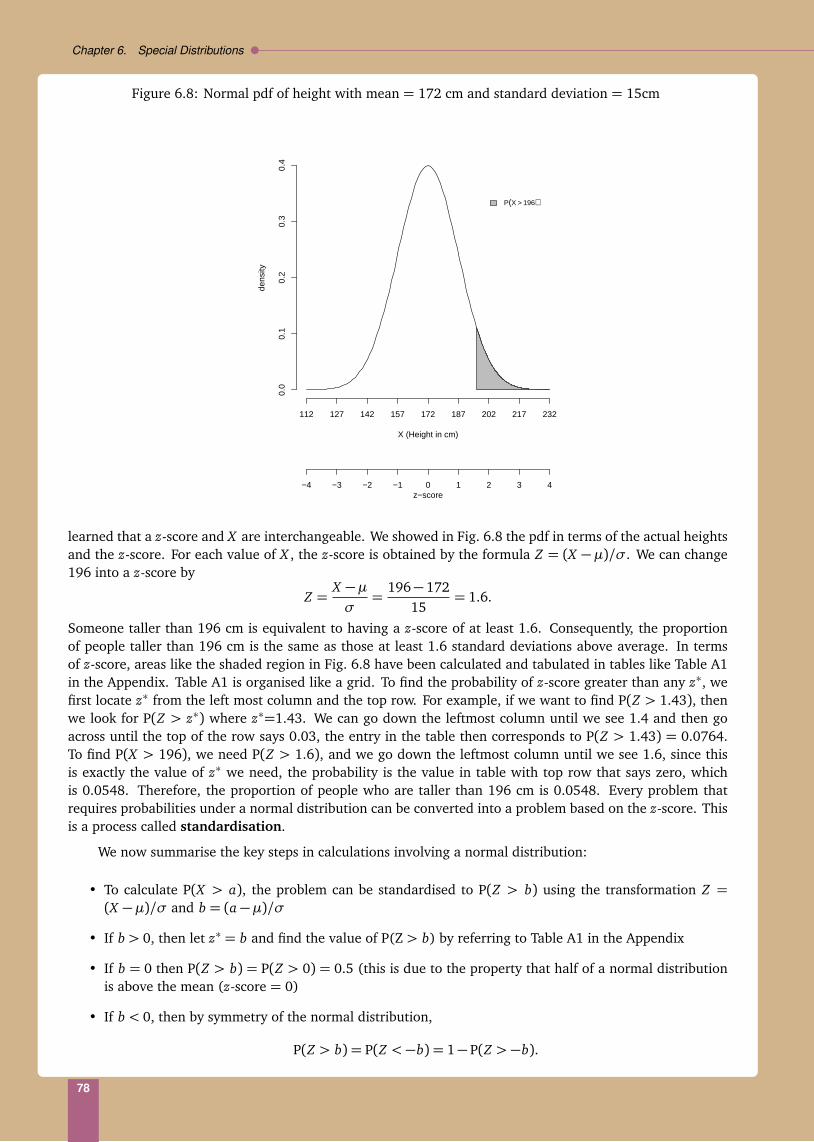
Chapter 6. Special Distributions
Figure 6.8: Normal pdf of height with mean = 172 cm and standard deviation = 15cm
X (Height in cm)
dens
ity
−4 −3 −2 −1 0 1 2 3 4
112 127 142 157 172 187 202 217 232
0.0
0.1
0.2
0.3
0.4
z−score
P(X > 196)
learned that a z-score and X are interchangeable. We showed in Fig. 6.8 the pdf in terms of the actual heightsand the z-score. For each value of X , the z-score is obtained by the formula Z = (X − µ)/σ. We can change196 into a z-score by
Z =X −µσ
=196− 172
15= 1.6.
Someone taller than 196 cm is equivalent to having a z-score of at least 1.6. Consequently, the proportionof people taller than 196 cm is the same as those at least 1.6 standard deviations above average. In termsof z-score, areas like the shaded region in Fig. 6.8 have been calculated and tabulated in tables like Table A1in the Appendix. Table A1 is organised like a grid. To find the probability of z-score greater than any z∗, wefirst locate z∗ from the left most column and the top row. For example, if we want to find P(Z > 1.43), thenwe look for P(Z > z∗) where z∗=1.43. We can go down the leftmost column until we see 1.4 and then goacross until the top of the row says 0.03, the entry in the table then corresponds to P(Z > 1.43) = 0.0764.To find P(X > 196), we need P(Z > 1.6), and we go down the leftmost column until we see 1.6, since thisis exactly the value of z∗ we need, the probability is the value in table with top row that says zero, whichis 0.0548. Therefore, the proportion of people who are taller than 196 cm is 0.0548. Every problem thatrequires probabilities under a normal distribution can be converted into a problem based on the z-score. Thisis a process called standardisation.
We now summarise the key steps in calculations involving a normal distribution:
• To calculate P(X > a), the problem can be standardised to P(Z > b) using the transformation Z =(X −µ)/σ and b = (a−µ)/σ
• If b > 0, then let z∗ = b and find the value of P(Z > b) by referring to Table A1 in the Appendix
• If b = 0 then P(Z > b) = P(Z > 0) = 0.5 (this is due to the property that half of a normal distributionis above the mean (z-score = 0)
• If b < 0, then by symmetry of the normal distribution,
P(Z > b) = P(Z < −b) = 1− P(Z > −b).
78

6.4. Normal distribution
Let z∗ = −b. Look up in Table A1, to find P(Z > z∗). Finally P(Z > b) = 1− P(Z > z∗).
Example 6.9Suppose the final score in STAT101 follows a normal distribution with mean= 70 and variance= 16 and that in STAT151follows a normal distribution with mean = 65 and variance = 25.(a) What is the probability that a student from STAT101 scores above 66?Let X denote the final score in STAT101, we are interested in finding P(X > 66). In this problem,
µ= 70,σ2 = 16,σ =p
σ2 = 4.
We first standardise the problem. Let a = 66, then
b =a−µσ=
66− 704
= −1.
Therefore, P(X > 66) = P(Z > −1).Since b < 0. We let z∗ = −b = −(−1) = 1. From Table A1, we obtain P(Z > z∗) = 0.1587. Finally, P(Z > −1) =1− P(Z > 1) = 1− 0.1587= 0.8413.(b) What is the probability that a student from STAT101 scores between 66 and 74?Let X denote the final score in STAT101, we are interested in finding P(X ∈ (66, 74)) = P(66 < X < 74) = P(X <74)−P(X < 66). We already obtained from (a) that P(X > 66) = 0.8413. Therefore, P(X < 66) = 1−0.8413= 0.1587.For P(X < 74), we first standardise. Let a = 74,
b =a−µσ=
74− 704
= 1,
so P(X < 74) = P(Z < 1) = 1 − P(Z > 1). From Table A1, P(Z > 1) = 0.1587. So P(Z < 1) = 0.8413. Therefore,P(X < 74)− P(X < 66) = 0.8413− 0.1587= 0.6826.(c) What is the probability that a student from STAT101 scores between 80 and 90?
P(80< X < 90) = P(X < 90)− P(X < 80)
= P
Z <90− 70
4
− P
Z <80− 70
4
= P(Z < 5)− P(Z < 2.5)∼= 1− P(Z < 2.5) (Since the largest value in Table A1 is 3 or so)
= 0.0062.
(d) Jonathan wants to be in the top 2.5% of his STAT101 class, what is the minimum, in terms of number of standarddeviations above the mean does he need to achieve?This problem is complementary to those we have done so far. Instead of finding the shaded area using Table A1, we arenow given the shaded area and asked to find the value of z∗ corresponding to the shaded region using Table A1. Theproblem is illustrated in Fig. 6.9.To find z∗, we use Table A1 and look for 0.025 in the interior of the table and then find the corresponding value ofz∗. An excerpt of the relevant section of the table is attached. The highlighted value gives 0.025 in the interior ofthe table, which corresponds to the intersection of the values 1.9 and 0.06, hence z∗ =1.9+0.06=1.96 corresponds toP(Z > z∗) = 0.025.
z∗ 0.00 0.01 0.02 0.03 0.04 0.05 0.06 0.07 0.08 0.09
0.0 0.5000 0.4960 0.4920 0.4880 0.4840 0.4801 0.4761 0.4721 0.4681 0.46410.1 0.4602 0.4562 0.4522 0.4483 0.4443 0.4404 0.4364 0.4325 0.4286 0.4247
...1.7 0.0446 0.0436 0.0427 0.0418 0.0409 0.0401 0.0392 0.0384 0.0375 0.03671.8 0.0359 0.0351 0.0344 0.0336 0.0329 0.0322 0.0314 0.0307 0.0301 0.02941.9 0.0287 0.0281 0.0274 0.0268 0.0262 0.0256 0.0250 0.0244 0.0239 0.0233
...In order to be in the upper 2.5% of the class, Jonathan has to be at least 1.96 standard deviation above the mean,corresponding to a z-score of 1.96. By symmetry, a z-score of −1.96 or lower would place a student in the lower 2.5% of
79

Chapter 6. Special Distributions
the class. Therefore, 95% of the population are in the interval, (µ−1.96σ,µ+1.96σ). This property holds for any normaldistribution.
(e) Jill is from STAT101, her final score is 64. Jack is from STAT151, his final score is 65. Who did better?
Since Jack and Jill are from different classes, it does not make sense to compare their actual score. Rather, it is better tocompare their scores relative to their own class. To do this, their z-scores can be calculated. For Jill,
Z =64− 70
4= −1.5,
for Jack,
Z =60− 65
5= −1.
Since the z-score of Jack is higher than that of Jill, Jack did relatively better. This example illustrates that z-scores areuseful for comparing values from different normal distributions.
Figure 6.9: Example 6.9(d)
X (STAT101 score)
dens
ity
−4 0 ? 4
54 70 ? 86
0.0
0.1
0.2
0.3
0.4
z−score
P(Z > z*)=.025
Sum and difference of Normal random variables
If X and Y are normal random variables with means µX and µY , respectively, then
X ± Y ∼ N(µX ±µY , Var(X + Y ))
80

7Sampling and sampling distribution
In Example 1.1, we reported a study (Foster et al., New England Journal of Medicine, 2003, 2082-90) designedto evaluate the effectiveness of a new diet in reducing weight. The study assembled a sample of 60 individualsand used them to infer about the diet’s effectiveness in the population. This study is an example of inferentialstatistics, the method by which inferences concerning a whole population are made from a sample. Inferentialstatistics is concerned with estimation and hypothesis testing. Estimation uses the data from samples toprovide estimates of various characteristics of the population, e.g., the mean weight loss in the populationor the proportion in the population who successfully lose more than 10 kilograms under the new diet. Inhypothesis testing, a hypothesis concerning the nature of the population is postulated. This hypothesis mayconcern the nature of the whole population or the value of a specific feature of the population. For example,we may be interested to test whether the new diet is more effective than the conventional diet in reducingweight in the population. Alternatively, it may be of interest to determine whether the average weight loss ismore than 10 kilograms if the new diet is used in the population.
7.1 Population and Sample
A population is defined as the set of all units of interest. We shall distinguish between two kinds of population– finite population and infinite population. A finite population is a population in which the total numberof units (members) in the population is enumerable. Examples of finite populations include the students ofa university, the airplanes owned by an airline, or the potential customers in a target market. A populationis usually considered infinite if counting the total number of units in population is impossible. Examples ofinfinite populations include the items manufactured by a company that plans to be in business forever, or allthe new inventions in the future.
A sample can be regarded as any subset of a population. A single member of a population can be asample of that population, even though such a sample is not considered to be a very good or useful sample inmost circumstances. We shall return to the discussion sample size later.
In practice, as long as (1) the sample size, n, and the population size, N are such that n/N < 0.05 (i.e.,no more than 5% of the population is sampled) or (2) the population size N so big to be considered infiniteor (3) sampling with replacement, then there is no difference in the statistical analyses between a finiteand an infinite population. Henceforth, we assume one or both of these conditions are satisfied so we do notdistinguish between the two types of population.
81

Chapter 7. Sampling and sampling distribution
Example 7.1
Suppose we wish to determine the most popular brand of soft drink sold last month, then the population would be everysoft drink sold last month. The units that make up the population must be described in terms of the characteristics thatclearly identify them for the purpose of the study. For example, assuming a sample of size n= 50 is used, then the unitsin the sample would look like: Coke, Coke, 7-Up, Sprite, 7-Up, Coke, etc. It is clear from the context that the populationsize, N could be very large and we can safely assume that n/N < 0.05.
7.2 Random Sampling
Sampling allows statisticians to draw conclusions about a whole (the population) by examining a part (thesample). It enables us to study characteristics of a population by directly observing a portion of the entirepopulation. We are not interested in the sample itself, but in what can be learned from the sample – and howthis information can be applied to the entire population.
It is essential that sampling be correctly planned and carried out. If the wrong questions are posed tothe wrong people, we will not receive information that will be useful when applied to the entire population.One sampling method commonly used to select a representative sample of the population, i.e., a samplethat allows us to draw valid conclusion about the population characteristic of interest, is simple randomsampling. Simple random sampling is a type of probability sampling. Probability sampling involves theselection of a sample from a population, based on the principle of randomization or chance. Randomizationensures that there is no preferential treatment in selection which may introduce selectivity bias. In simplerandom sampling, each unit of the population has an equal chance of being selected. If this condition is trulysatisfied when selecting a sample, then the principles of probability will allow us to draw valid inferences aboutthe population. These conditions may be modified in order to allow for unequal probabilities of selection ofdifferent members of a population, as in other types of sampling plans such as stratified sampling or clustersampling. As long as the probability of selection for each member of a population can be determined, themethods of inferential statistics can be applied.
We assume that members in the sample are independently drawn from the population. This condition issatisfied under simple random sampling from an infinite population and can be made to be satisfied in othersituations. Independence means that a member of the sample has no influence on the other members, as faras the characteristic of interest is concerned. Requiring independence makes sense since we want each unit tocontribute a separate piece of information about the characteristic of interest and not repeating informationalready provided by other units in the sample. For example, if the interest is to study household income inthe population, it is pointless to ask every member of the same household to report the household income,because they all give the same information.
In this set of course notes, only the case of simple random sampling of independence observations isdiscussed and we shall refer it simply as random sampling. When we say we have a random sample, we meanthe sample has been drawn under these conditions.
In Section 7.1, we mentioned that if sampling is carried out with replacement, then irrespective ofthe population size, the population can be treated as infinite. Here, we elaborate on that point and wedistinguish sampling with replacement with another type of sampling called sampling without replacement.For sampling with replacement, we assume that when we sample a unit from a population, the unit will be“returned" to the population so it can potentially be drawn again into the same sample. For sampling withoutreplacement, once a unit is drawn, it will not be returned back to the population, so a unit cannot appear morethan once in the same sample. When we sample with replacement, any two sample values are independent.Practically, this means that what we sample first does not affect what we get on the next unit to be drawn. Insampling without replacement, the two sample values aren’t independent. Practically, this means that whatwe obtain in the first draw affects what we can get for the second draw. The distinction between these twotypes of sampling schemes is especially important when the population size is finite and small.
82

7.3. Parameter and statistic
7.3 Parameter and statistic
Suppose the characteristic we want to study is the household income in a population. Then each householdin the population need to be identified by its income. The population consists of units such as $5600, $4600,$7400, $6500, etc.. Household incomes in the population form a distribution. The distribution tells us theprobabilities associated with different values of household income in the population as well as summariessuch as the mean, variance, range, or proportion (probability) of households that have income higher than$10000, etc.. Quantities such as the mean and the variance in a population are referred to as parameters.
In practice, the probability distribution of a characteristic is seldom known unless the characteristic hasbeen measured on every unit of the population, i.e., a census has been carried out. Instead, a random samplefrom the population can be selected and the characteristic is observed on each unit of the sample. Quantitiessuch as the mean and the variance are also defined for a sample. We called these quantities statistics. Asopposed to parameters in a population which are usually unknown, statistics can be calculated from the sampleonce it has been taken. A statistic is often used to estimate an unknown parameter. Specifically, we estimateunknown population quantities based on their respective known sample counterparts.
Example 7.2
We wish to study the household income in a population. We assume household income in the population has a finitemean of µ and finite variance of σ2, and both are unknown. Suppose the population has N households, then we canimagine that the household incomes are X1, ...., XN , and they are not known unless we take a census. By definitionthe population mean and variance of the household income are given by µ = 1
N
∑Ni=1 X i and σ2 = 1
N
∑Ni=1(X i − X )2,
respectively. Suppose a random sample of n households from the population is drawn and their incomes X1, ..., Xn arerecorded,a then we can calculate two statistics: (1) the sample mean, X = 1
n
∑ni=1 X i and (2) the sample variance,
s2 = 1n−1
∑ni=1(X i − X )2. These statistics are intuitive counterparts of the unobserved population parameters µ and σ2,
and can be used to estimate these parameters.
Before we proceed further, let us take a moment to look at some population quantities and their respectivesample counterparts.
Table 7.1: Some common population quantities and sample counterparts
Population parameter Sample counterpartProbability distribution Histogram(Population) mean, µ (Sample) mean, X(Population) variance, σ2 (Sample) variance, s2
(Population) standard deviation, σ (Sample) standard deviation, s(Population) proportion (Sample) proportion
7.4 Sampling error
When we try to use a sample to infer about a population, it will be subject to what is known as samplingerror. Sampling error arises from estimating a population parameter by looking at only one portion of thepopulation rather than the entire population. It refers to the difference between the estimate derived from asample and the “true" value that would result if a census is carried out under the same conditions. There isno sampling error in a census because the calculations are based on the entire population.
For populations such that the analyses follow those of an infinite population, sampling error only depends:
83

Chapter 7. Sampling and sampling distribution
1. sample size
2. variability of the characteristic of interest in the population
As a general rule, the more number of units being sampled (larger sample size), the smaller the samplingerror will be. In Example 7.2, a random sample with n= 100 households would have a smaller sampling errorthan a random sample of n = 25 households from the same population. To understand why the sample sizen is related to the sampling error, we only need to recognize that, if we take the average of a large number ofhouseholds, some of which have income higher than µ and some lower than µ, then the high and low incomeswill tend to cancel out in the sample average, resulting in a small sampling error.
The greater the difference between the population units, the larger the sample size is required to achievea specific level of reliability. To understand why sampling error depends on the variation in the contextof Example 7.2, let us consider the following scenarios. First, imagine a population where the variation inhousehold income is very small (e.g., from $4,000 to $5,000), then income is unlikely to be very different fromhousehold to household and few of them would be different from the population average µ. In that case, theaverage income in a random sample is unlikely to be very different from µ since the individual householdincomes are not too different from µ. On the other hand, for a population where the range in householdincome is very large (e.g., from $5000 to $50000), household incomes are likely to be very different fromeach other and also very different from µ. In that case, the average income in a random sample of the samesize is more likely to be different from µ since the individual household incomes can be quite different fromµ.
Population size plays an almost non-existent role in sampling error as far as large populations areconcerned.
Example 7.3 (Continued from Example 7.2)
In using the sample mean X and the sample variance, s2 to estimate the unknown population parameters µ and σ2, thesampling errors are X −µ and s2 −σ2, respectively.
Suppose that n = 4 households are randomly selected and their income are: X1 = 5600, X2 = 4600, X3 = 7400,X4 = 6500. From these observations, we calculate X = (5600 + 4600 + 7400 + 6500)/4 = 6025 and s2 = (5600 −6025)2+(4600−6025)2+(7400−6025)2+(6500−6025)2/3= 142500, then the sampling errors using this particularsample to estimate µ and σ2 would be 6025−µ and 142500−σ2, respectively.
Notice that both the sample mean X and the sample variance s2 depend on the values of each of the n observations.Hence, X and s2 can be interpreted as summarizing the information contained in the sample, which in turn are used todraw inferences about the entire population, which has not been completely observed.
7.5 Sampling distribution
In the preceding section, we discussed how using a sample statistic to infer a population parameter will incursampling error. We defined sampling error as
Sampling error = Sample statistic − Population parameter
which in the context of estimating a population mean µ using a sample mean X , the sampling error becomesX−µ. In Example 7.2, the sample mean from the data is X = 6025 and so the sampling error becomes 6025−µ.We would like to find out the value of the sampling error so we can evaluate how well we are estimating µ.Unfortunately, since µ is not known, we will never know what is the actual value of our sampling error.
Even though we do not know precisely the sampling error of our sample statistic, it does not stop us fromstudying its behaviour. For example, we may try to find out whether the sampling error is likely to be big.
Random sampling is carried out based on the principle of randomization and chance. Hence, if we wereto draw a random sample of size n from a population of size N , then any of the N units in the population
84

7.5. Sampling distribution
would have the same chance of being selected into the sample. In fact, using simple random sampling, thereare
Nn
possible ways of selecting a sample of size n from a population of size N . For example, if N = 10000and n = 4, then
Nn
=10000
4
≈ 4.164167 × 10¹⁴. Our sample is one of theN
n
possible samples of size nfrom the population. For each of these
Nn
samples, a statistic can be calculated and each will have its ownsampling error. The possible values of the statistic and its sampling error form distributions called samplingdistributions. A sampling distribution gives the probabilities of different values of the statistic and its samplingerror, and hence offers a glimpse of the behaviour of our own sample statistic and its sampling error.
We begin by considering the sampling distribution of the sampling error. Recall the Normal distributionwas introduced as a distribution for measurement errors. In our context, we are using a sample mean toestimate a population mean. Our statistic comes from a random sample we have chosen and it is one ofthe many possible statistics that could have been used, had other samples of the same size been drawn. Foreach random sample from the same population, the statistic will incur a sampling error, but it will have thecharacteristics of a measurement error and therefore, we may conjecture the sampling distribution of thesampling error to be a Normal distribution.
Next we turn to the sampling distribution of X . Notice that Sampling error= X−µ but µ is the populationmean and it does not change no matter what sample is taken. Hence, the sampling distribution of the X shouldbe the same as the sampling distribution of the sampling error except for a translation of the unknown µ. Sowe also conjecture the sampling distribution of X to be Normal.
The conjectures we made in the preceding paragraphs turn out to be true, and the results are summarizedin an important theorem called the Central Limit Theorem (CLT).
Central Limit Theorem (CLT)
Suppose there are n independent observations of X from a population with finite mean µ and finitevariance σ2. If n is reasonably big (≥ 30), the sampling distribution of the sample mean X is approximately
Normal with mean = µ and variance = σ2
n
standard deviation= σpn
. Furthermore, the sampling
distribution of the sampling error of X is Normal with mean zero and variance the same as that in the samplingdistribution of X .
By the CLT, if we constructed histograms of X and its sampling error from different random samples, wewould see the empirical sampling distributions look like Figure 7.1. Notice that the two sampling distributionshave exactly the same shape, except the centers are translated. This phenomenon is not a coincidence; rather,it is the result of the earlier discussion, that the differences in sampling errors between samples is the same asthe differences in sample statistics.
Figure 7.1: Sampling distributions of (a) X and (b) its sampling error
(a) X
µ
(b) Sampling error
0
85

Chapter 7. Sampling and sampling distribution
Explanation
When we use X to estimate µ, we will never know the size of the sampling error in our estimate. However,the CLT says that the size of the sampling error follows a Normal distribution and it allows us to evaluate theprobabilities of sampling errors of different sizes.
The distribution of X around µ follows a Normal distribution with variance= σ2
n . A small variance meansthat there is little chance that X will be very different from µ, hence the sampling error will likely be small.Conversely, a large variance suggests there is a greater chance that X will be quite different from µ, hence thesampling error could be large.
So far, we have not mentioned how the variance of the sampling distribution is derived in the CLT. Wenow attempt to answer this question. According to the CLT,
σ2
n= Var(sampling error)= Var(X −µ) = Var(X )
︸ ︷︷ ︸
(since µ is constant)
in different random samples from the population. We now derive the variance of the sampling error. LetX1, ..., Xn be the n observations of X selected into our sample. Recall that which n members in the populationwill be drawn is completely random. For example, X1, the first unit selected into the sample, is unpredictable.The only information we know about X1 is it is a unit from the population. Hence, we called X1 a randomvariable. The same idea of randomness applies to X2, ..., Xn. Since our sample is random, it makes sense tospeak of the variance of the sample mean X = (X1+X2+ ...+Xn)/n, which is a function of X1, ...., Xn. Hence:
Var(sampling error)= Var(X ) = Var
X1 + ...+ Xn
n
=1n2
Var(X1 + ...+ Xn)
=1n2
Var(X1) + ...+ Var(Xn)︸ ︷︷ ︸
X1,...,Xn are independent
=1n2
n× Var(X )︸ ︷︷ ︸
The distribution of X has variance σ2
=1n2
nσ2
=σ2
n.
The last expression suggests that the variance of the sampling error (and that of the statistic X ) is (1) directlyproportional to σ2, which by definition is the variation of the characteristic X under study and (b) inverselyproportional to the sample size n. Hence, our derivation here proves our claims in Chapter 7.4.
We will revisit the concepts of sampling error and sampling distributions in Chapter 9.
86

8Estimation
In the pandemic example of Chapter 2, we obtained data from 100 patients treated on drug A. Out of thesepatients, 60 recovered but the remaining 40 did not, despite having received treatment. The natural questionto ask is: “How effective is treatment A? This question implies not only the effectiveness of A on the sample,but also that on the population of all future patients with the same disease. Our intention is to use what welearned from our sample, to answer this question about the population of patients.
We learned in Chapters 1-6 the device that links our sample to the population is a probability model.In Chapter 6.1, we argued that each patient, when treated, gives one of two outcomes: recovers (1) or doesnot recover (0). We can imagine an underlying probability, p, for recovery and 1− p for no recovery, and wemay assume the value of p is identical for all patients– everyone has the same chance of recovery – then ourprobability model for the outcome of a treated patient is:
Outcome Probability1 (recovers) p
0 (does not recover) 1− p
In other words, the outcomes in our sample are outcomes of Bernoulli trials (Chapter 6.1). Recall fromChapter 2.2 that probabilities represent population proportions, hence, 0 < p < 1 represents the populationproportion of patients who recover, if treated with A. In Fig. 8.1, we show plots of the probability distributionfunction (pdf) of the model under three different values of p = 0.5,0.6, 0.3. For example, when p = 0.5,the pdf shows the (population) proportion of recovery is exactly the same as that for no recovery, whereaswhen p = 0.3, the proportion of recovery is much lower than that of no recovery. From Chapter 6.1, p is theparameter of the Bernoulli trial.
8.1 Maximum likelihood estimation
Fig. 8.1 shows only three possible models, there are many more to consider. In fact, since the parameter p isonly known to lie in (0,1), there are infinitely many possible models. However, we are only interested in onetreatment, A, and there is only one population– the population of all patients with the same disease. Hencewe wish to search for one model (one value of p) that best describes the effect of A on the population.
Our search is based on the premise that, since our sample is a subset of the population and it is our onlyknowledge about the population, the model that is the most likely explanation for what we have seen in thesample would also be the most likely model for the population. This idea leads to a method called maximum
87

Chapter 8. Estimation
Figure 8.1: Three possible models for pandemic data
0 1
X
P(X
)
01
p = 0.5
0 1
X
P(X
)
01
p = 0.6
0 1
X
P(X
)
01
p = 0.3
likelihood estimation, abbreviated as MLE.a
Before we describe MLE, we define some notations. We let X be the random variable of interest. Wedenote the sample of n observations of X by X1, ..., Xn. In the remainder of this set of notes, we make theassumption that when we have a sample of size n, the observations in the sample are all independent of eachother. This means, for example, the outcome of one patient is unaffected by those of other patients. We willuse the Greek letter θ (pronounced “theeta") as a generic symbol for any parameter. In the past few chapters,we have used P(x) to denote pdf for a discrete random variable and f (x) for a continuous random variable.In this chapter, we use the common notations f (x |θ ) to denote pdf and F(x |θ ) to denote cdf, whether Xis discrete or continuous, where the inclusion of θ means the model depends on the parameter θ . In thepandemic example, θ = p, and the model obviously depends on the value of θ , see, e.g., Fig. 8.1.
In the pandemic example, we use the sample to “guess" the value of p for the population, we call ourguess of p an estimate. From here on, we denote an estimate of a parameter θ by θ .
In the literature, the following sentence: “X1, ..., Xn iid (independently and identicallydistributed) f (x |θ )" is often used as a shorthand to describe the situation above, that we have a sample of nobservations of X from a population with model f (x |θ ).
We now explain MLE using the pandemic example.
Example 8.1
We observed a sample of n= 100 treatment outcomes: (X1, ..., Xn)=(1, 1, 1, 0, 0, ..., 0, 1, 1), where in total 60 recovered(1) and 40 did not (0). We assume X , the treatment outcome in the population follows a Bernoull i(p) distribution, butp is unknown. Based on the data, what is the most likely value of p?
Let us consider a few possible values of p : 0.01, 0.5 and 0.99.
If p = 0.01, then the chance of the first patient recovers is 0.01. The same chance applies to the second patient, and soon. Since we made the assumption that outcomes are independent, the probability of observing the data, is precisely:
(0.01)(0.01)(0.01)(0.99)(0.99) · · · (0.99)(0.01)(0.01) = (0.01)60(0.99)40 ≈ 6.7× 10−121.
so if p = 0.01, it is almost impossible to see the data. Based on this calculation, we argue that p is unlikely to be 0.01.
aRonald Aylmer (R.A.) Fisher, 1890-1962 suggested the maximum likelihood method in 1912 when he was a third yearundergraduate student at Cambridge University
88

8.1. Maximum likelihood estimation
Similarly, p is also unlikely to be 0.99 since, if p = 0.99, almost certainly all patients in our sample would recover. Infact, if p = 0.99, the chance of observing the data is
(0.99)(0.99)(0.99)(0.01)(0.01) · · · (0.01)(0.99)(0.99) = (0.99)60(0.01)40 ≈ 5.5× 10−81.
Finally, if p = 0.5, then the chance of observing the data would be
(0.5)(0.5)(0.5)(0.5)(0.5)(0.5)(0.5)(0.5)(0.5)(0.5) = 0.5100 ≈ 7.9× 10⁻³¹,
which is still small, but nevertheless much higher than the previous two values. So out of these three values, the valueof p that is most consistent with the data is 0.5. Having said that, we understand that p can be any value between 0and 1 so there are many other possibilities we have not considered. We shall formalise the way to find p. In above, wecompared different values of p by evaluating the probability of observing the data, for each value of p. We continuealong that line by writing down a general expression for the probability of observing the data, for any value of p, asfollows:
The probability that the first observation is 1 is p.
The probability that the second observation is 1 is p.
The probability that the third observation is 1 is p.
The probability that the fourth observation is 0 is 1− p, etc.,
The probability that (X1, ..., Xn)=(1, 1, 1, 0, 0, ..., 0, 1, 1) is
L(p|X1, ..., Xn) = L(p|X1)× L(p|X2)× ...× L(p|Xn−1)× L(p|Xn)= p× p× p× (1− p)× (1− p)× · · · × (1− p)× p× p
= p60(1− p)40.
L(p|X1, ..., Xn) is a function of p. If there is no danger of confusion, then L(p|X1, ..., Xn) is simply written as L(p). Insteadof calling it a probability, we call L(p) a likelihood function and it can be considered the “likelihood of a particular valueof p given the observed data". The maximum likelihood estimate (also abbreviated as MLE) of p, is the value of p thatgives the highest likelihood of p given the observed data.
We formalise the above procedure by trying a range of values of p in (0,1). Among the values we chose, L(p) is highestat p = 0,6, so it is the most likely value of p, among those in the table, for the population.
p L(p) = p60(1− p)40
0 0
0.1 1.4× 10−62
0.2 1.5× 10−46
0.3 2.7× 10−38
0.4 1.8× 10⁻³³
0.5 7.9× 10⁻³¹
0.6 5.9× 10⁻³⁰
0.7 6.2× 10⁻³¹
0.8 1.7× 10⁻³⁴
0.9 1.8× 10−43
1.0 0
We note from the table that the magnitude of L(p) is very small for all values of p. That is the result of multiplyingtogether a lot of probabilities, each between 0 and 1. Sometimes, that can create numerical problems, and hence, inpractice, we often take the natural logarithm of L(p) to obtain a log-likelihood, `(p),
`(p) = logL(p)= 60log(p) + 40log(1− p).
We plot L(p) and `(p) for values of p ∈ (0, 1) in Fig. 8.2. We observe that both figures start with low values, peak at thesame point, p = 0.6, and then descend. The value where L(p) or `(p) peaks is the MLE of p given the data. Notice thatFig. 8.2 is not a plot of pdf’s.
An alternative way to find the MLE is to use Calculus. We observe from Fig. 8.2 that the MLE is where L(p) or `(p) peaks,or in other words, when the functions are temporarily not increasing or decreasing. In Calculus, such a point is where
89

Chapter 8. Estimation
the derivative of the function is zero. Based on this argument, we define the derivatives d L(p)dp ≡ L′(p) and d`(p)
dp ≡ `′(p)
, then the MLE p is found by eitherL′(p) = 0 or `′(p) = 0.
We illustrate using both here, though in practice, only one of them is sufficient since they always give the same solution.Starting with L′(p),
L′(p) = 60p59(1− p)40 − 40p60(1− p)39
= p59(1− p)39[60(1− p)− 40p],
then p is the point where L′(p) is zero, i.e.,
L′(p) = p59(1− p)39[60(1− p)− 40p] = 0
60− 60p− 40p = 0
p =60
100= 0.6.
Using `′(p), we have
`′(p) = 601p− 40
11− p
.
p is the point where `′(p) is zero:
`′(p) = 601p− 40
11− p
= 0
60(1− p)− 40p = 0
60− 60p− 40p = 0
p =60
100= 0.6
Hence, we show that the MLE p = 0.6 whether we use Fig. 8.2 or Calculus.
Figure 8.2: Likeihood vs. log-likelihood for pandemic data
0.0 0.2 0.4 0.6 0.8 1.0
0e+
002e
−30
4e−
306e
−30
Likelihood
p
p60(1
−p)
40
0.0 0.2 0.4 0.6 0.8 1.0
−25
0−
200
−15
0−
100
Log−likelihood
p
60lo
g(p)
+40
log(
1−
p)
We now formally define the MLE using n independent observations X1, ..., Xn from a population. Thelikelihood function of θ given X1, ..., Xn is:
L(θ ) = f (x1|θ )× ...× f (xn|θ ) =n∏
i=1
f (x i|θ ).
90
8.1. Maximum likelihood estimation
The log-likelihood is obtained by taking the natural logarithm of L(θ ),
`(θ ) = logL(θ )=n∑
i=1
log f (x i|θ )
To obtain the MLE, we differentiate the likelihood or log-likelihood with respect to θ ,
L′(θ ) =d L(θ )
dθor `′(θ ) =
d`(θ )dθ
.
The MLE of θ is then the solution to
L′(θ ) = 0 or `′(θ ) = 0.
Example 8.2
Table 8.1 records the time (T) between major earthquakes in 1900-1979. A histogram of the data is given in Fig. 8.3.We may assume T follows an Ex p(λ) distribution. However, we do not know what value of λ gives an exponentialdistribution that best describes T . We can use likelihood method to find the MLE of λ. There are n= 62 observations ofT in the data. The likelihood for λ based on the data is:
L(λ) =n∏
i=1
f (t i |λ) =n∏
i=1
λe−t iλ
Taking logarithm gives,
`(λ) =n∑
i=1
log
λe−t iλ
=n∑
i=1
[log(λ)− t iλ]
= nlog(λ)−λn∑
i=1
t i .
Since we only need to using one of Ł(λ) or `(λ), we choose to work with `(λ). We differentiate `(λ) with respect to λ,
`′(λ) =nλ−
n∑
i=1
t i .
The MLE λ is the solution to `′(λ) = 0, so
`′(λ) = 0
n
λ−
n∑
i=1
t i = 0
n
λ=
n∑
i=1
t i
λ =n
∑ni=1 t i
=1t
≈ 0.00229.
91

Chapter 8. Estimation
Figure 8.3: Histogram of earthuqake data in Example 8.2
Days
Pro
port
ion
0
0 400 800 1200 1600 2000
f(t) = λe−λt
Table 8.1: Days between major earthquakes 1900-1979
840 157 145 44 33 121 150 280 434736 584 887 263 1901 695 294 562 72176 710 46 402 194 759 319 460 40
1336 335 1354 454 36 667 40 556 99304 375 567 139 780 203 436 30 384129 9 209 599 83 832 328 246 1617638 937 735 38 365 92 82 220
8.1.1 Invariance property of MLE’s
In Example 8.2, if we assume time between major earthquakes follows an Ex p(λ) distribution, then likelihoodmethod tells us the most likely model that explains T is when λ = 0.00229. That model allows us to answerquestions about time to major earthquakes. For example, we might be interested in the average time betweenmajor earthquakes, i.e., E(T ), or we might wish to determine whether the next major earthquake would bewithin a year from the last one, i.e., P(T ≤ 365). Based on an Ex p(λ) distribution (see Chapter 6.3),
E(T ) =1λ
,
P(T ≤ 365) = F(365) = 1− e−365λ.
So in our questions, we are not directly interested in λ. Rather, we wish to determine functions of λ. Followingour discussion of MLE’s, naturally we would like to find the MLE of E(T ) and P(T < 365). In other words, weseek the most likely values of E(T ) and P(T ≤ 365), given the data. Thanks to a property called the invarianceproperty, the solution is surprisingly simple if we already know the MLE λ.
The invariance property of MLE says:
If θ is the MLE of θ , then for any function, g(θ ), the MLE of g(θ ) is g(θ )
According to the invariance property, we do not need to work out the MLE’s for E(T ) and P(T ≤ 365)from scratch, as we did for λ; rather, we simply plug the MLE λ into the expressions for these quantities. Weillustrate this process with the following example.
Example 8.3 (Continued from Example 8.2)
We found the MLE for λ is λ= 0.00229, hence the MLE’s for E(T ) and P(T ≤ 365) are, respectively,
bE(T ) =1
λ
=1
1/ t= t
≈ 437 Days,
bP(T ≤ 365) = 1− e−365λ
≈ 1− e−365(0.00229)
≈ 0.57.
92

8.1. Maximum likelihood estimation
8.1.2 Non-standard conditions
In Example 8.2, each of the observations in the sample is a time, i.e., days between earthquakes. Hence,every observation gives us the same amount of information about a typical unit (Days between earthquakes)in the population. Sometimes, data are collected such that some observations do not offer the same amountof information about a typical unit in the population. For example, we might wish to include earthquakes inancient times that are not very precisely recorded, then our sample would include a mixture of observations,offering different amounts of information about the best model for T . In such cases, the likelihood method canstill be used, except that the likelihood (or the log-likelihood) function need to be written down differently.We summarise the discussion below. Suppose we have independent observations X1, ..., Xn such that X i iseither an observation of X or a function of X . The likelihood function of θ given X1, ..., Xn is:
L(θ ) = L(θ |X1, ..., Xn) = L(θ |X1)× ...× L(θ |Xn)≡n∏
i=1
L(θ |X i).
We illustrate calculating the MLE under non-standard conditions using Example 8.4.
Example 8.4 (Continued from Example 8.2)
Suppose in addition to the 62 observations, we have an additional observation from historical records and we only know,T63 > 2650. Write ( t1, t2, ..., t62, t63) = (t1, t2, ..., t62, t63 > 2650). Using all 63 observations, the likelihood becomes
L(λ) = L(λ| t1, ..., t63) =63∏
i=1
L(λ| t i)
=62∏
i=1
f ( t i |λ)× L(λ| t63)
=62∏
i=1
f (t i |λ)× P(2650< t63|λ)︸ ︷︷ ︸
=1−F(2650|λ)
`(λ) =62∑
i=1
log[ f (t i |λ)] + log [1− F(2650|λ)]
=62∑
i=1
log
λe−t iλ
+ log
e−2650λ
= 62log(λ)−λ62∑
i=1
t i − 2650λ
Taking derivative with respect to λ,
`′(λ) =62λ−
62∑
i=1
t i − 2650.
The new MLE λ is the solution to
`′(λ) = 0
62
λ−
62∑
i=1
t i − 2650 = 0
λ =
∑62i=1 t i + 2650
62≈ 480.
93

Chapter 8. Estimation
8.2 Evaluating estimates
Whenever we make a guess of an unknown, the natural question we ask ourselves is: “How good is ourguess?". Based on the same idea, when we use a sample to come up with a model for the population, wewould like to find out how good is our model. In the pandemic example, we used data from 100 patients toarrive at the MLE p = 0.6, of the success probability of A, if it was applied to the population of patients. Weunderstand the MLE is based on a sample, which is only a subset of the population. Hence, we call the MLEan estimate for the reason that we do not fully expect the MLE to be exactly the same as the true, but unknownp. In other words, we expect
p︸︷︷︸
estimate
− p︸︷︷︸
parameter
6= 0.
The difference p − p is called a sampling error. A sampling error results because we use only a sample, ora subset, of the population to estimate the entire population. Intuitively, we wish to determine this samplingerror so we could adjust our estimate to obtain a better guess of the parameter p. But since p is unknown,hence, there is no way we can determine the exact value of our sampling error. In other words, we cannot tellexactly how far 0.6 is from p.
To solve this conundrum, instead of inquiring “How far is 0.6 from p?", we ask “How good is MLE as amethod for estimation?". If the answer to this second question is “Yes", then we should believe 0.6 is a goodestimate of p, otherwise, we probably should not trust our estimate.
When MLE is being evaluated as a method for estimation, we call it an estimator. Hence an estimator isa method, when applied to a sample, gives an estimate. The way we evaluate MLE as an estimation methodis by studying its average performance assuming it is used repeatedly on different random samples from thepopulation.
Before we carry out our evaluation, we first define the problem in more general terms. Suppose we wishto estimate an unknown parameter θ using a particular method (estimator). Let θ denote a typical estimatewhen the estimator is applied to a random sample of size n from the population.
From our discussion earlier, for each sample,
one sample︷ ︸︸ ︷
θ − θ = sampling error= ?
where the unknown sampling error is not estimable. Instead of looking at the sampling error of each samplein isolation, we evaluate the overall performance of the estimator for all possible samples that could be drawnfrom the population. We will use three measures for evaluation; they are listed below and will be discussedin greater detail in the next few sections. Notice for each measure, we use the concept of expectation fromChapter 5. Recall that expectation is an average, so we will be taking average performance over differentsamples.
many samples︷ ︸︸ ︷
E(θ − θ ) = “Average sampling error”E[θ − E(θ )2] = “Average spread of estimates between samples”
E[(θ − θ )2] = “Average squared sampling error”
8.2.1 Bias
The bias of an estimator is the average sampling error of its estimates over different samples:
Bias(θ ) = E︸︷︷︸
average
(θ − θ ).
An estimator is unbiased if Bias(θ ) = 0. Otherwise, it is biased. An unbiased estimator is an estimatorsuch that the average sampling error is zero. A biased estimator either has a tendency to overestimate orunderestimate θ .
94

8.2. Evaluating estimates
Some estimators are biased when the sample size n is small but Bias(θ )→ 0 for large values of n. Thoseestimators are called consistent estimators. In practice, it is often sufficient to look for a consistent ratherthan an unbiased estimator.
The difference between a biased and an unbiased estimator is illustrated in Fig. 8.4. In the figure, twoestimators are applied to different random samples of a population. For each sample, each estimator producesa x-mark. The biased estimator (bottom panel) has a tendency to give a lot of x-marks that are overestimatesof θ . The unbiased estimator (top panel) also incurs sampling errors, since the x-marks do not land on θ . Thisis to be expected, since sampling errors are unavoidable whenever we based our estimates on samples. Whatdifferentiates this unbiased estimator from the biased estimator is there is no tendency for too many x-marksabove θ (overestimate) or too many below θ (underestimate).
Figure 8.4: Biased vs. unbiased estimator in repeated samples
Estimates from different samples
θθUnbiased
θBiased
8.2.2 Variance
If we have an unknown, and if an estimator gives very different estimates simply because different randomsamples are taken from the same population, for the this unknown, then the method cannot be good.Therefore, a second way to assess an estimator is the spread of its estimates under different random samples.We learned in Chapter 1 that a measure of spread is the variance.
The variance of an estimator is given by:
Var(θ ) = E︸︷︷︸
average
[θ − E(θ )2].
Another name for Var(θ ) is the sampling variation. Var(θ ) is a measure of the stability of an estimatorwhen it is applied to different random samples. An estimator with a small value for Var(θ ) tends to producesimilar estimates from different random samples whereas an estimator with a large variance tends to producevery different estimates from different random samples for the same unknown θ . An estimator with a largevariance is undesirable. However, a small variance does not guarantee that the estimator is good, see below.
The difference between an estimator with small variance and one with large variance is illustrated inFig. 8.5. Similar to the situation in Fig. 8.4, two estimators are applied to different random samples of apopulation. For each sample, each estimator produces a x-mark. The bottom panel estimator has a large spreadof x-marks, indicating its tendency to give very different estimates of the same unknown θ . Comparatively,the spread of x-marks is very small for the top panel estimator, indicating it tends to give similar estimates forthe same unknown θ .
Figure 8.5: Estimators with large vs. small variance in repeated samples
Estimates from different samples
E(θ )θSmall variance
θLarge variance
Note that in Fig. 8.5, the reference is E(θ ), not θ , so an estimator with a small variance only means theestimator gives similar estimates from different samples, but there is no guarantee any of these estimate willbe close to the unknown θ . This is why we argued earlier that a small variance is not a confirmation of a goodestimator. We therefore, need the next concept, see Chapter 8.2.3, to complete our evaluation of an estimator.
95
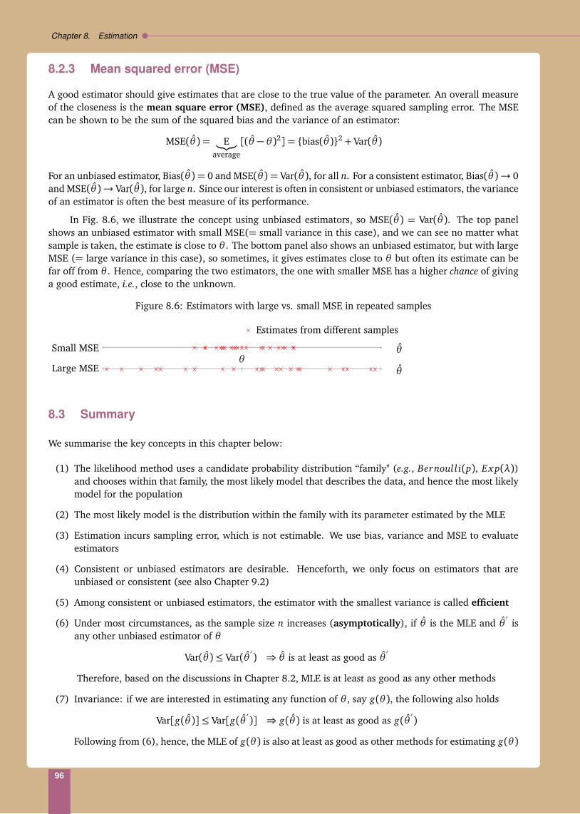
Chapter 8. Estimation
8.2.3 Mean squared error (MSE)
A good estimator should give estimates that are close to the true value of the parameter. An overall measureof the closeness is the mean square error (MSE), defined as the average squared sampling error. The MSEcan be shown to be the sum of the squared bias and the variance of an estimator:
MSE(θ ) = E︸︷︷︸
average
[(θ − θ )2] = bias(θ )2 + Var(θ )
For an unbiased estimator, Bias(θ ) = 0 and MSE(θ ) = Var(θ ), for all n. For a consistent estimator, Bias(θ )→ 0and MSE(θ )→ Var(θ ), for large n. Since our interest is often in consistent or unbiased estimators, the varianceof an estimator is often the best measure of its performance.
In Fig. 8.6, we illustrate the concept using unbiased estimators, so MSE(θ ) = Var(θ ). The top panelshows an unbiased estimator with small MSE(= small variance in this case), and we can see no matter whatsample is taken, the estimate is close to θ . The bottom panel also shows an unbiased estimator, but with largeMSE (= large variance in this case), so sometimes, it gives estimates close to θ but often its estimate can befar off from θ . Hence, comparing the two estimators, the one with smaller MSE has a higher chance of givinga good estimate, i.e., close to the unknown.
Figure 8.6: Estimators with large vs. small MSE in repeated samples
Estimates from different samples
θθSmall MSE
θLarge MSE
8.3 Summary
We summarise the key concepts in this chapter below:
(1) The likelihood method uses a candidate probability distribution “family" (e.g., Bernoull i(p), Ex p(λ))and chooses within that family, the most likely model that describes the data, and hence the most likelymodel for the population
(2) The most likely model is the distribution within the family with its parameter estimated by the MLE
(3) Estimation incurs sampling error, which is not estimable. We use bias, variance and MSE to evaluateestimators
(4) Consistent or unbiased estimators are desirable. Henceforth, we only focus on estimators that areunbiased or consistent (see also Chapter 9.2)
(5) Among consistent or unbiased estimators, the estimator with the smallest variance is called efficient
(6) Under most circumstances, as the sample size n increases (asymptotically), if θ is the MLE and θ′
isany other unbiased estimator of θ
Var(θ )≤ Var(θ′) ⇒ θ is at least as good as θ
′
Therefore, based on the discussions in Chapter 8.2, MLE is at least as good as any other methods
(7) Invariance: if we are interested in estimating any function of θ , say g(θ ), the following also holds
Var[g(θ )]≤ Var[g(θ′)] ⇒ g(θ ) is at least as good as g(θ
′)
Following from (6), hence, the MLE of g(θ ) is also at least as good as other methods for estimating g(θ )
96

9Estimation
In the pandemic example of Chapter 2, we obtained data from 100 patients treated on drug A. Out of thesepatients, 60 recovered but the remaining 40 did not, despite having received treatment. The natural questionto ask is: “How effective is treatment A? This question implies not only the effectiveness of A on the sample,but also that on the population of all future patients with the same disease. Our intention is to use what welearned from our sample, to answer this question about the population of patients.
We learned in Chapters 1-6 the device that links our sample to the population is a probability model.In Chapter 6.1, we argued that each patient, when treated, gives one of two outcomes: recovers (1) or doesnot recover (0). We can imagine an underlying probability, p, for recovery and 1− p for no recovery, and wemay assume the value of p is identical for all patients– everyone has the same chance of recovery – then ourprobability model for the outcome of a treated patient is:
Outcome Probability1 (recovers) p
0 (does not recover) 1− p
In other words, the outcomes in our sample are outcomes of Bernoulli trials (Chapter 6.1). Recall fromChapter 2.2 that probabilities represent population proportions, hence, 0 < p < 1 represents the populationproportion of patients who recover, if treated with A. Based on the data from our sample, it is natural touse the sample proportion of recoveries as an estimate of p. Let p denote our sample estimate of p thenp = 60/100 = 0.6. We call this estimate a point estimate of p. A point estimate uses a single number as anestimate of an unknown. Our discussion in Chapter 7.4 suggests that, since our point estimate is obtainedfrom a subset of the population of patients, there is a chance of sampling error. Sampling error is simply thedifference between our estimate p = 0.6 and the unknown p. In this chapter, we examine how to acknowledgethe possibility of sampling errors when we report estimates. The kind of estimates we consider is calledconfidence interval estimate or simply interval estimate.
An interval estimate combines a point estimate with an error estimate. In the context of the pandemicexample, instead of using the point estimate p = 0.6 for p, an interval estimate of p has the form
(p− a, p+ a),
for some a > 0. The quantity a is called a margin of error. The margin of error reflects the uncertainty in ourestimate due to sampling error. Thus, in an interval estimate p ± a, we predict the unknown p to lie withinthe interval. Obviously, the wider the interval, the more certain we are that p would lie within the interval.Hence, in an interval estimate, we adjust the interval width to reflect our confidence level that the unknownwould lie within the interval. If we wish to be 99% certain that the unknown lies in our interval estimate,then we need to make the interval wider than if we are satisfied with a 90% certainty, etc..
97

Chapter 9. Estimation
Our question is: “How do we determine the value of a?"
9.1 Large sample confidence intervals
In Chapter 7.5, we argued that sampling error in an estimate is not known precisely in any particular problem.To evaluate an estimate, we study the behaviour of the method used to obtain the estimate. Our estimatep = 0.6 is based on a particular random sample of n= 100 patients. Based on the CLT (Chapter 7.5), p fromdifferent random samples of the same size would behave like Fig. 9.1 (compare this to Fig. 7.1, which illustratesthis situation using a histogram). Estimates p from different random samples form a sampling distribution.Fig. 9.1 (or Fig. 7.1) shows that, just because of random sampling, we may not obtain an estimate p that isexactly the same as p, the quantity of interest. However, we show by using this sampling distribution, alongwith the CLT, we can find the value of a, and hence a confidence interval estimate of p.
p
Estimates p from different samples
Figure 9.1: Estimates p of p using different random samples
Assume the sample size of n = 100 is sufficiently large, then the CLT tells us estimates p from differentsamples in Fig. 9.1 follow a normal distribution with mean p and variance Var(p), see Fig. 9.2. Since variancemeasures spread, hence Var(p) measures the spread of p from different random samples of the population.If we take the square root of Var(p), we obtain the standard deviation of p. The standard deviation of anestimate based on a sample is often called a standard error and is usually abbreviated as SE. Hence, we writeSE(p) =
p
Var(p).
Figure 9.2: Sampling distribution of p
p
Estimates from different samples
Recall from our discussion of the normal distribution in Chapter 6.4, that there is a set of empirical rulesthat applies to every normal distribution. In particular, for any normal distribution, approximately 95% ofthe values fall within ±1.96 standard deviation of the mean. Applying this fact to the current problem, wecan say that, in approximately 95% of the random samples, p would be within ±1.96SE(p)a from p. We nowtranslate this sentence as follows:
p− 1.96SE(p)< p < p+ 1.96SE(p)
⇒ p− 1.96SE(p)− p < p− p < p+ 1.96SE(p)− p (subtract p throughout)
⇒ −1.96SE(p)< p− p < 1.96SE(p)
⇒ −1.96SE(p)− p < p− p− p < 1.96SE(p)− p (subtract p throughout)
⇒ −1.96SE(p)− p < −p < 1.96SE(p)− p
⇒ p− 1.96SE(p)< p < p+ 1.96SE(p) (multiply by −1 throughout and reverse the “< " signs)
aSometimes 1.96 is replaced by 2 for convenience
98
9.2. Large sample confidence interval for a population mean
The last expression above leads to the statement:
“We are 95% certain that p is within p± 1.96SE(p)"
This statement gives us a 95% confidence interval for p. Hence, we found that by choosing a = 1.96SE(p),we can be 95% certain that the unknown p would lie within the interval p± a. The lower and upper boundsof this confidence interval are called, respectively, the lower and upper confidence limits. Our level ofconfidence is 95% and 1.96SE(p) is the margin of error.
As discussed at the beginning of this chapter, we adjust the interval width to find interval estimates withdifferent levels of confidence. For example, since approximately 99% of the values in any normal distributionfall between ±2.58 standard deviations of its mean, we could follow similar steps as before to arrive at p ±2.58SE(p) for a 99% confidence interval for p. We notice that the forms of the 99% and 95% confidenceintervals are identical, the only difference being the multiplier of 2.58 vs. 1.96.
Two important considerations when reporting an interval estimate are: the interval width and theconfidence level. A short interval width is desired because it allows us to locate the unknown in a narrowinterval. A higher confidence level is preferred so we have more confidence that the unknown actually fallswithin the interval. Comparing the 95% and 99% confidence intervals we derived earlier, we observe thatthe 99% confidence interval is wider, but giving us a higher confidence that p lies within the interval. Thiscomparison highlights the following dilemma. In any interval estimate, we cannot simultaneously shorten thewidth while increasing the confidence level; a decision must be made to balance between the two criteria. Inpractice, the most commonly used confidence level is 95%, which is the level we adopt here.
The method for forming an interval estimate for p generalises to finding interval estimates for anyquantity θ in a population.
Large sample 95% confidence interval estimate
Given a sufficiently large random sample (of n independent observations) from a population, let θ bethe sample estimate of a population characteristic θ . If θ is obtained from a well behaved estimator, then anapproximate 95% confidence interval for θ is given by
θ ± 1.96SE(θ )
9.2 Large sample confidence interval for a population mean
One of the most important characteristics of a population is the population mean. For example, we mightbe interested in determining the average hours of work among women in a population, or the mean #kids < 6 years in each family in a population. Here, we investigate how to obtain interval estimates for apopulation mean. Towards the end of Chapter 9.1, we gave an approximate 95% confidence interval for anypopulation characteristic θ . We apply that result to find approximate 95% confidence intervals here. Let µ bethe population mean of interest, and let µ be a sample estimate of µ, then an approximate 95% confidenceinterval for µ is:
µ± 1.96SE(µ).
A natural estimator for a population mean is the sample mean, X . Suppose we have a sample of n observationsof X : X1, ..., Xn and the sample mean is X . Replacing µ by X , an approximate 95% confidence interval estimatefor µ is:
X ± 1.96SE(X ),
where the margin of error is 1.96SE(X ). We now work out the margin of error. Recall that SE(X ) =p
Var(X ),where in Var(X ), “Var" measures how X changes if it is applied to different random samples. From Chapter 7.5,
99
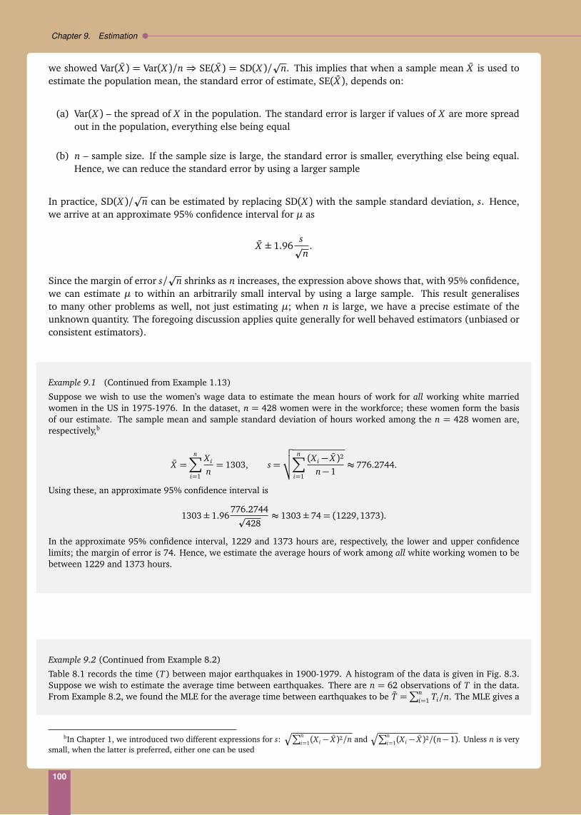
Chapter 9. Estimation
we showed Var(X ) = Var(X )/n ⇒ SE(X ) = SD(X )/p
n. This implies that when a sample mean X is used toestimate the population mean, the standard error of estimate, SE(X ), depends on:
(a) Var(X ) – the spread of X in the population. The standard error is larger if values of X are more spreadout in the population, everything else being equal
(b) n – sample size. If the sample size is large, the standard error is smaller, everything else being equal.Hence, we can reduce the standard error by using a larger sample
In practice, SD(X )/p
n can be estimated by replacing SD(X ) with the sample standard deviation, s. Hence,we arrive at an approximate 95% confidence interval for µ as
X ± 1.96sp
n.
Since the margin of error s/p
n shrinks as n increases, the expression above shows that, with 95% confidence,we can estimate µ to within an arbitrarily small interval by using a large sample. This result generalisesto many other problems as well, not just estimating µ; when n is large, we have a precise estimate of theunknown quantity. The foregoing discussion applies quite generally for well behaved estimators (unbiased orconsistent estimators).
Example 9.1 (Continued from Example 1.13)
Suppose we wish to use the women’s wage data to estimate the mean hours of work for all working white marriedwomen in the US in 1975-1976. In the dataset, n = 428 women were in the workforce; these women form the basisof our estimate. The sample mean and sample standard deviation of hours worked among the n = 428 women are,respectively,b
X =n∑
i=1
X i
n= 1303, s =
√
√
√
n∑
i=1
(X i − X )2
n− 1≈ 776.2744.
Using these, an approximate 95% confidence interval is
1303± 1.96776.2744p
428≈ 1303± 74= (1229, 1373).
In the approximate 95% confidence interval, 1229 and 1373 hours are, respectively, the lower and upper confidencelimits; the margin of error is 74. Hence, we estimate the average hours of work among all white working women to bebetween 1229 and 1373 hours.
Example 9.2 (Continued from Example 8.2)
Table 8.1 records the time (T) between major earthquakes in 1900-1979. A histogram of the data is given in Fig. 8.3.Suppose we wish to estimate the average time between earthquakes. There are n = 62 observations of T in the data.From Example 8.2, we found the MLE for the average time between earthquakes to be T =
∑ni=1 Ti/n. The MLE gives a
bIn Chapter 1, we introduced two different expressions for s:q
∑ni=1(X i − X )2/n and
q
∑ni=1(X i − X )2/(n− 1). Unless n is very
small, when the latter is preferred, either one can be used
100

9.3. Large sample confidence interval for a population proportion
point estimate, which is T ≈ 437.2 days. To find a 95% confidence interval, we need
SE(T ) =SD(T )p
n
≈sp
n
=
q
∑ni=1(Ti − T )2/(n− 1)
pn
≈ 50.78.
Hence an approximate 95% confidence interval for the average time between earthquakes is:
T ± 1.96SE(T )≈ 437.2± 1.96(50.78)≈ (337.6, 536.7).
In this example, there is an alternate solution. Suppose we assume T follows an Ex p(λ) distribution, then since underan exponential distribution E(T ) = 1/λ = SD(T ), hence an alternate way to estimate SD(T ) is simply T ! In that case,SE(T ) can estimated by 437.2/
p62≈ 55.52, which leads to the following alternate 95% confidence interval:
437.2± 1.96(55.52)≈ (328.4,546.0).
Both of these confidence intervals are valid. The former only makes the assumption that the sample size is large, so thatthe CLT can be used. The latter makes an additional assumption that T follows an exponential distribution.
9.3 Large sample confidence interval for a population proportion
In Chapter 9.1, we examined using a sample proportion, p from n= 100 patients, to estimate p, the probability(or proportion) of success if the treatment were given to all patients in the population. We found a generalexpression for an approximate 95% confidence interval for p. We now return to complete the problem. Beforewe do that, we wish to understand the meaning of a population proportion.
Let X be the treatment outcome of a patient from the population, such that
X =
1 recovers0 does not recover
.
Denote the population size by N , and suppose the value of X in the population are X1 = 1 (recovers), X2 = 0(does not recover), X3 = 0, ... ,XN = 1, which is a collection of 1’s and 0’s.c Then p is defined as
p =#1′s
N
=1+ 0+ 0+ · · ·+ 1
N
=X1 + X2 + X3 + · · ·+ XN
N≡ µ.
Hence, p is a special case of the population mean µ in Chapter 9.2, with only 1’s and 0’s. This analysis showsthat we can use the results in Chapter 9.2 to find an approximate 95% confidence interval for p. Suppose asample of (sufficiently large) n patients are treated, then their treatment outcomes X1, ..., Xn are
1 with probability p0 with probability 1− p
.
Furthermore, the sample proportion p of successful outcome is
p =X1 + · · ·+ Xn
n≡ X
cIn practice, the values of X1, ..., XN are unknown to us. But it does not affect our study of the meaning of p
101

Chapter 9. Estimation
then an approximate 95% confidence interval for p is
p± 1.96SE(p) ⇔ X ± 1.96SE(X ) ⇔ X ± 1.96SD(X )p
n.
In this case, however,
Var(X ) = E(X 2)− E(X )2
= (1)2p+ (0)2(1− p)− [(1)p+ (0)(1− p)]2
= p− p2
= p(1− p)
⇒ SD(X ) =Æ
p(1− p)
⇒ SE(p) = SE(X ) =
p
p(1− p)p
n.
In practice, we need to estimate SE(p) byp
p(1− p)/n. Hence, an approximate 95% confidence interval forp is:
p± 1.96
p
p(1− p)p
n.
Example 9.3
In the pandemic example, we obtained p = 60/100= 0.6 from n= 100 patients. Hence an approximate 95% confidenceinterval for p is
0.6± 1.96
p
0.6(0.4)p
100≈ 0.6± 0.096= (0.504, 0.696).
9.4 Confidence interval for a normal population mean
The confidence intervals in Chapter 9.1-9.3 are for large samples, when the CLT applies. For small samples,there are no general expressions for confidence interval estimates. One exception is when we wish to find aninterval estimate of a normal population mean µ. In that case, for any n, an approximate 95% confidenceinterval for µ is:
X ± 1.96SE(X ) = X ± 1.96SD(X )p
n.
This interval, however, is not that useful in practice because it requires us to know the population standarddeviation, SD(X ). A natural solution is to replace SD(X ) by the sample standard deviation, s. This approachworks for large n since in that case, we revert back to the confidence interval in Chapter 9.2 (That interval isbased on the CLT, which applies to any population, including normal). For small sample size, however, thisapproach does not work well, since then s may have substantial sampling error in estimating SD(X ). Due tothis second source of sampling error (in addition to the sampling error of X as an estimate for µ), we needto stretch the confidence interval to maintain the same confidence level that µ would fall within the interval.The stretching is done by replacing 1.96 by a value t, t > 1.96 from a table called the t-table (Table A.2). Theamount of stretching depends on how well s estimates SD(X ), which in turns depends on n. We summarisethe procedure below.
102

9.4. Confidence interval for a normal population mean
95% confidence interval estimate for a normal population mean
For a random sample of n independent observations from a normal population, an approximate 95%confidence interval for the population mean µ is given by
X ± tsp
n
where t is a quantity depending on n. Values of t can be obtained from Table A.2.
Example 9.4
Assume household expenditure in a population follows a normal distribution. Suppose expenditure from n = 10households are obtained: 1874, 1642, 1603, 1931, 2103, 2068, 1948, 1798, 2364, 1918. Based on the data, wefind
X = 1924.9, s =
√
√
√
∑ni=1(X i − X )2
n− 1≈ 223.1021.
To find an approximate 95% confidence interval for the population mean household expenditure, we need to use a tvalue from Table A.2. The t value depends on a quantity called the degrees of freedom (d f ), defined as d f = n− 1.Values of t for selected d f s are given below
d f = n− 1 6 7 8 9 10 20 120 >120value 2.447 2.365 2.306 2.262 2.228 2.086 1.98 1.96
In this example, n= 10, which gives d f = 10−1= 9; so we choose the value 2.262 in the table to replace 1.96 to arriveat an approximate 95% confidence interval of
1924.9± 2.262223.1021p
10≈ 1924.9± 159.5= (1765.4, 2084.4),
which is wider than an interval using 1.96. However, by stretching the interval, we are assured of the 95% confidencelevel that µ falls within (1765.4, 2084.4).
103

10Hypothesis Testing
Studies are often carried out to answer questions such as: “Do married women with kids < 6 years workdifferent hours than typical working married women?" or “Do incentive and support programs help to improvestudent performance?". These questions could be approached by setting up appropriate hypotheses and usingdata to test the hypotheses. To answer the first question, for example, we could specify a null hypothesis,denoted as H0, that the average hours worked in working women with kids < 6 years, µ, equals µ0 and testit against an alternative hypothesis, denoted H1 or HA, that µ 6= µ0, where µ0 is the average hours workedfor a typical working married woman.
Using the women’s wage data from Chapter 1, we observe, among n= 53 working white married womenwith kids< 6 years, their average hours of work (X ) in 1975 was X ∗ = 965.3774. (Notice that we have placeda superscript ∗ upon the usual notation X . For the remaining part of this chapter, we will use this conventionfor any quantity we obtained from the sample we observed, the reason for this convention will be made clearin Chapter 10.1) We also know from census, that the average hours worked was 1300 for all working marriedwomen in 1975. Comparing the two figures, we clearly see a difference in average hours worked between thetwo types of women. If so, can we reject H0 and accept H1? The answer is “not yet". We could argue that965.3374 is a sample mean, and the observed difference may be due to sampling error, see Chapter 8.2 and9.1. Here, we learn how a statistical test resolves this issue in testing the hypotheses of interest.
10.1 Large sample tests
To begin, we state the hypotheses as follows:
H0 : µ= 1300 vs. H1 : µ 6= 1300
We notice that in the hypotheses, µ refers to the population of working married women with kids < 6 years,whereas we observed a sample. This is precisely the reason why we cannot base on the observation that thesample mean, X ∗ 6= 1300, to reject H0.
Intuitively speaking, we may assume H0 : µ = 1300 is true and then determine whether the observeddata look plausible under that assumption. If the answer is “Yes", then there is no reason to question thatµ= 1300. On the contrary, if the data are unlikely to have been observed under µ= 1300, then we may castdoubts on H0 and instead, accept H1 : µ 6= 1300. This simple intuition underpins all statistical tests we study.
Recall in Chapter 9.1, the central limit theorem (CLT) states that, if we have a population with mean µ=1300, then the sample mean, X , from different random samples (of sufficiently large size n) follow a normaldistribution with mean µ and standard error SE(X ) = SD(X )/
pn. This situation is illustrated in Fig. 10.1.
This distribution is sometimes called the null distribution. Notice a null distribution is simply a sampling
104

10.1. Large sample tests
distribution discussed in Chapter 9 when data are drawn under the null hypothesis. A null distribution recordsthe distribution of sample characteristics when samples are drawn from a population under the null hypothesis,H0.
Before we carry on, we now make clear of the distinction between X and X ∗. Recall from that X ∗ is themean of the sample we obtained, whereas X is the sample mean of a random sample from the population underH0. Hence, SE(X ) = SD(X )/
pn refers to the standard error of X of a random sample from the population
under H0.
Figure 10.1: Null distribution of X
1300
X from different samples
In our problem, we may assume n= 53 is sufficiently large. Then if our sample is from a population withµ = 1300, we expect its sample mean to be like one of x-marks. On the contrary, if our sample mean is farfrom the x-marks in Fig 10.1, then we suspect our sample does not behave like a sample from a populationwith µ= 1300.
The null distribution is N(µ = 1300, SE(X ) = SD(X )/p
53). Recall that SE(X ) refers to the standarderror of the sample mean of a random sample (of n= 53) from a population with µ= 1300. Hence it shouldbe calculated using information from the population with µ = 1300. Often, however, as in this case, thereis no other information on the population with µ = 1300 and SE(X ) = SD(X )/
p53 is unknown. To solve
this problem, even though we don’t know whether our sample comes from the population with µ= 1300, weestimate SD(X ) by the sample standard deviation of our sample, s∗ = 851.8106.ab. Hence, an approximationto the null distribution is N(1300, s∗/
p53≈ 117).
Recall our discussion of z-score from Chapter 6.4, we can calculate
z∗ =X ∗ − 1300
SE(X )≈
965.3374− 1300117
≈ −2.86.
This z-score tells us that our sample’s X ∗ = 965.3774 is approximately 2.86 standard deviations from X of atypical random sample from a population with µ= 1300. This z-score is often called a test statistic.
To determine how X ∗ compares to X of a typical random sample from a population with µ = 1300, wedo the following. We let Z = (X − 1300)/SE(X ) be the z-score for a random sample from a population withµ = 1300. Hence Z is a z-score for one of x-marks in Fig 10.1. We find the probability that a z-score “asdifferent as" z∗ by
P(Z ≤ −2.86 or Z ≥ 2.86) = P(Z ≤ −2.86) + P(Z ≥ 2.86) = 2× P(Z > |2.86|) = 2× 0.0021︸ ︷︷ ︸
Table A.1
= 0.0042,
which is very small. Our analysis shows that X ∗ of our sample is very different from X of a typical randomsample from a population with µ= 1300. We deduce that
either
(a) our sample comes from a population with µ= 1300 but it is a very unusual sample(with probability no more than 0.0042 that our sample comes from the population)
(b) our sample comes from a population with µ 6= 1300
Since 0.0042 is a very low probability, we are inclined to believe (a) may not be correct, and we reject H0.
aWe used s∗ = 1n−1
∑ni=1(X i − X )2 here
bWe require that s∗ is an unbiased estimate of SD(X )
105

Chapter 10. Hypothesis Testing
10.2 Null and alternative hypotheses
We now formally define the null and the alternative hypotheses. In every hypothesis testing situation, the twohypotheses are:
(1) Null hypothesis (H0) — e.g., µ= 1300 in the women’s wage example
(2) Alternative hypothesis (H1 or HA) — the opposing hypothesis — e.g., µ 6= 1300 in the women’s wageexample.
The hypotheses are set up so that H0 usually represents some norm or standards. We assume H0 to be trueunless there is strong evidence against it. In the women’s wage example, we questioned H0 because there isoverwhelming evidence against it (there is only ≤ 0.0042 probability that a sample mean of 965.3374 wouldbe observed if H0 is true). Since we set-up the test by assuming H0 to be true, therefore, H0 cannot be provento be true. As such, a hypothesis that we wish to prove must be framed as H1.
Example 10.1
a. Suppose a government wishes to show increasing the frequency of mammography screening would reduce breastcancer mortality. Let p and p0 be, respectively, the mortality rate due to breast cancer, with and without increasedscreening frequency. The hypotheses may be set up as follows:
H0 : p ≥ p0 vs. H1 : p < p0.
In this case, the norm is increased screening frequency does not reduce cancer mortality (p ≥ p0). We assume thisis true unless proven otherwise and it is stated as H0. In the alternative, we assume increased screening frequencyreduces mortality, hence p < p0
b. Do men and women earn different wages? We can answer this question by comparing the average wages betweenmen and women. If we let these averages be µM and µF , respectively, then we may write the hypotheses as:
H0 : µF = µM vs. H1 : µF 6= µM .
In this case, unless we have evidence otherwise, we assume the average wages are the same between men andwomen, hence H0 states that µF = µM . The alternative simply states their averages are different, women couldmake more, or they could make less.
c. Suppose in a pandemic, the disease incidence rate is 1/1000 (one out of every 1000 people is infected) and a drugcompany wants to show that its vaccine reduces incidence. If p denotes the incidence following vaccination, thenthe drug company would be interested to test:
H0 : p ≥1
1000vs. H1 : p <
11000
.
H0 assumes the vaccine does not reduce incidence (and may even lower immunity!), unless proven otherwise,hence p is at least 1/1000. The company wishes to show vaccination lowers incidence, hence the alternativehypothesis states that p < 1/1000.
10.3 p-value
In the women’s wage example, we found that the probability of observing values at least as unusual as theobserved sample mean X ∗ = 965.3774 is 0.0042. The value 0.0042 is sometimes called a p-value. A p-valuegives the probability of observing outcomes at least as unusual as the given data, if H0 is true.
106

10.4. Type I error
A p-value is a probability, therefore, 0 ≤ p-value ≤ 1. A p-value is sometimes simply written as p.c Ap-value is commonly used as evidence against H0. The lower the p-value, the more unlikely the observed datawould appear under H0, hence a low p-value is a strong evidence against H0.
Example 10.2
a. “A survey on 5716 women aged 24 years or below and 3782 women above 24 years showed that 66% of youngerwomen are in the labour force compared to 72% for the older women (p < 0.0001)". The survey results canbe interpreted as follows. H0 states that labour force participation is the same for both groups of women in thepopulation. The p-value refers to the chance of observing a difference of 72−66= 6 % in the two groups of womenin the samples, when H0 is true, i.e., there is actually no difference between the two groups in the population.However, the p-value < 0.0001 suggests a difference of 6% is unlikely to be observed if the two groups are thesame in the population. The p-value thus gives evidence that there may be a difference in labour participation ratebetween younger and older women in the population. In other words, there is evidence against H0.
b. “A study of the impact of an education program on school enrolment in rural areas shows that the average numberof hours of school attendance was 15 before and 15.2 following the program in a random sample of school children(p = 0.28)". In this study, H0 states that the program does not lead to higher enrolment hours. The study wishes toestablish a positive impact from the program, hence the alternative hypothesis would be an increase in enrolmenthours due to the program. The p-value says that the observed difference of 15.2−15= 0.2 hours would be observedwith a 28% chance even when the program does not make an impact. Since this chance is not particularly small,we may attribute the observed difference to sampling error (chance) and retain H0 that the program does not havean impact on school enrolment.
10.4 Type I error
In the women’s wage example, we rejected H0 : µ = 1300 because the chance of observing X ∗ = 965.3774is no more than 0.0042 (0.42%) if we assume H0 is true. When we reject H0, it is important to realise that,even though the data provide strong evidence against H0, there is still a 0.42% chance that our sample couldhave come from a population with µ = 1300. In other words, there is a 0.42% chance that we could haveincorrectly rejected the null hypothesis. The probability that a null hypothesis is wrongly rejected is called atype I (1) error (sometimes denoted by the Greek alphabet α, pronounced “alpha").
When a null hypothesis is rejected based on a small p-value, the chance of making a type I error has thesame value as the p-value. In the women’s wage example, the chance of a type I error is 0.0042.
10.5 Statistical significance and significance tests
In a statistical test, a small p-value means that there is a small probability that the data would be observed,if H0 is true. Thus we may choose to reject H0 when a small p-value is observed. However, there is no cleardefinition of what is considered “small" for a p-value.
A formal way to decide whether to reject H0 is called a significance test. In a significance test, H0 wouldbe rejected if the p-value falls below certain predetermined significance level. A commonly used significancelevel is 0.05, which leads to the following decision rules:
reject H0 if p-value < 0.05retain H0 if p-value ≥ 0.05
cA common mistake is to confuse a p-value with the parameter p in Bernoull i(p) or Binomial(n, p).
107
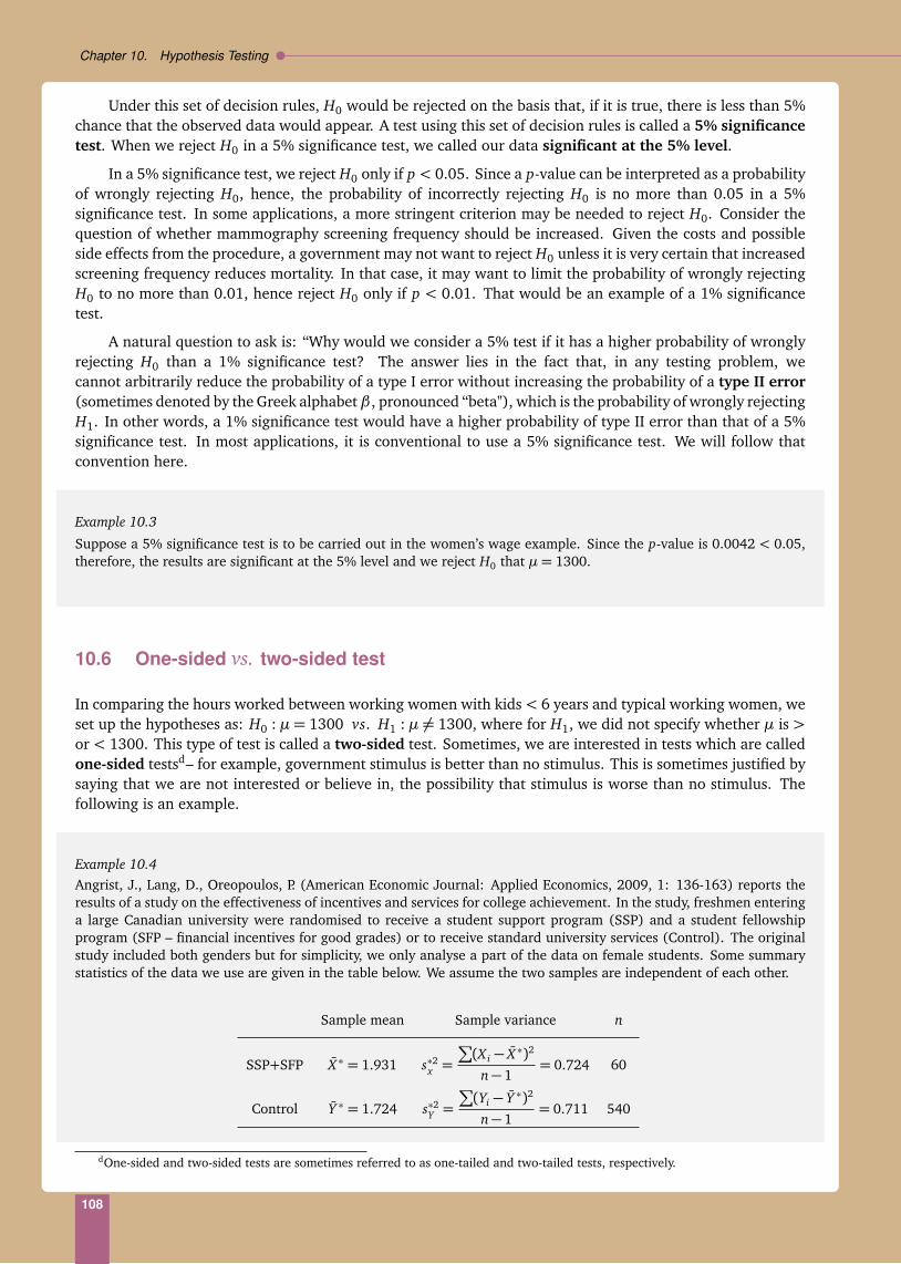
Chapter 10. Hypothesis Testing
Under this set of decision rules, H0 would be rejected on the basis that, if it is true, there is less than 5%chance that the observed data would appear. A test using this set of decision rules is called a 5% significancetest. When we reject H0 in a 5% significance test, we called our data significant at the 5% level.
In a 5% significance test, we reject H0 only if p < 0.05. Since a p-value can be interpreted as a probabilityof wrongly rejecting H0, hence, the probability of incorrectly rejecting H0 is no more than 0.05 in a 5%significance test. In some applications, a more stringent criterion may be needed to reject H0. Consider thequestion of whether mammography screening frequency should be increased. Given the costs and possibleside effects from the procedure, a government may not want to reject H0 unless it is very certain that increasedscreening frequency reduces mortality. In that case, it may want to limit the probability of wrongly rejectingH0 to no more than 0.01, hence reject H0 only if p < 0.01. That would be an example of a 1% significancetest.
A natural question to ask is: “Why would we consider a 5% test if it has a higher probability of wronglyrejecting H0 than a 1% significance test? The answer lies in the fact that, in any testing problem, wecannot arbitrarily reduce the probability of a type I error without increasing the probability of a type II error(sometimes denoted by the Greek alphabet β , pronounced “beta"), which is the probability of wrongly rejectingH1. In other words, a 1% significance test would have a higher probability of type II error than that of a 5%significance test. In most applications, it is conventional to use a 5% significance test. We will follow thatconvention here.
Example 10.3
Suppose a 5% significance test is to be carried out in the women’s wage example. Since the p-value is 0.0042 < 0.05,therefore, the results are significant at the 5% level and we reject H0 that µ= 1300.
10.6 One-sided vs. two-sided test
In comparing the hours worked between working women with kids < 6 years and typical working women, weset up the hypotheses as: H0 : µ= 1300 vs. H1 : µ 6= 1300, where for H1, we did not specify whether µ is >or < 1300. This type of test is called a two-sided test. Sometimes, we are interested in tests which are calledone-sided testsd– for example, government stimulus is better than no stimulus. This is sometimes justified bysaying that we are not interested or believe in, the possibility that stimulus is worse than no stimulus. Thefollowing is an example.
Example 10.4Angrist, J., Lang, D., Oreopoulos, P. (American Economic Journal: Applied Economics, 2009, 1: 136-163) reports theresults of a study on the effectiveness of incentives and services for college achievement. In the study, freshmen enteringa large Canadian university were randomised to receive a student support program (SSP) and a student fellowshipprogram (SFP – financial incentives for good grades) or to receive standard university services (Control). The originalstudy included both genders but for simplicity, we only analyse a part of the data on female students. Some summarystatistics of the data we use are given in the table below. We assume the two samples are independent of each other.
Sample mean Sample variance n
SSP+SFP X ∗ = 1.931 s∗2x =
∑
(X i − X ∗)2
n− 1= 0.724 60
Control Y ∗ = 1.724 s∗2Y =
∑
(Yi − Y ∗)2
n− 1= 0.711 540
dOne-sided and two-sided tests are sometimes referred to as one-tailed and two-tailed tests, respectively.
108

10.6. One-sided vs. two-sided test
Let µX ,µY be, respectively, the average first year GPA if all (female) students were to receive SSP+ SFP and standardservices (populations). The hypotheses can be set up as:
H0 : µX ≤ µY vs. H1 : µX > µY ⇔ H0 : µX −µY ≤ 0 vs. H1 : µX −µY > 0
Under H0, we assume SSP+SFP is no better than control, whereas in H1, SSP+SFP is better than control. This test isset-up as a one-sided test on the basis that we believe SSP+SFP cannot be worse than standard services, and we wish todetermine whether there is sufficient evidence to support SSP+SFP is better.
To test the hypotheses, we first replace H0 by H∗0, as follows:
H∗0 : µX −µY = 0 vs. H1 : µX −µY > 0
We can replace H0 : µX − µY ≤ 0 with H∗0 : µX − µY = 0 because if we conclude µX − µY > 0, we also mean µX − µY >−10,> −20, etc..
Following the women’s wage example, we first assume H∗0 is true. Under H∗0, µX −µY = 0, hence, grades from the twopopulations (SSP+SFP and control) are interchangeable. If we takes pairs of independent samples (of sufficiently largesizes), one from each of the two populations, then the sample mean difference, X − Y , from different pairs of samplesfollow a normal distribution with mean 0 and standard deviation SE(X − Y ). This situation is illustrated in Fig. 10.2.This distribution is the null distribution of the difference in sample means. We now find the test statistic:
z∗ =X ∗ − Y ∗ − 0SE(X − Y )
=X ∗ − Y ∗ − 0Æ
Var(X − Y )=
X ∗ − Y ∗√
√
√
Var(X ) + Var(Y )︸ ︷︷ ︸
Var(A−B)=Var(A)+Var(B) if A, B are independent
=X ∗ − Y ∗
√
√Var(X )60
+Var(Y )
540
≈X ∗ − Y ∗
√
√
√ s∗2X
60+
s∗2Y
540
=1.931− 1.724
√
√0.72460
+0.711540
≈ 1.79
In deriving the above test statistic, we made the commonly used assumption that s∗X and s∗Y are valid estimates of SD(X )and SD(Y ).To determine whether our data come from two populations with µX = µY , we do the following. We let Z = (X −Y )/SE(X − Y ) be the z-score for a pair of random samples from two populations with identical means. Hence Z is az-score for one of x-marks in Fig 10.2. We find the probability that a z-score “as high as" z∗ by
P(Z ≥ 1.79) = 0.0367︸ ︷︷ ︸
Table A.1
= p-value.
Notice here, unlike in Example 10.2, when we calculated the p-value, we were looking for “as different as", whereashere, we are looking for “as high as". Hence, all we need is to find P(Z ≥ 1.79).Based on our calculations, only 3.67% of the random samples from two identical populations would behave like oursample.
If we use a 5% significance test, then since p = 0.0367 < 0.05, we would reject H0, and conclude that students onSSP+SFP have a significantly higher GPA than those on standard university services.
109

Chapter 10. Hypothesis Testing
Figure 10.2: Null distribution of X − Y in Example 10.4
0
X − Y from different pairs of samples
10.7 Test statistic and critical values
In analysing woman’s wage of Example 10.2, we found the test statistic z∗ = −2.86. The value of |z∗| = 2.86is a measure of how far X ∗ is from X of a typical sample from the population under H0.
From Example 10.2 and invoking the CLT, if we take a random sample from a population under H0, i.e.,with µ= 1300, there is only a probability of 0.05 that X from that sample would fall outside 1300±1.96SE(X ),or |Z = (X − 1300)/SE(X )| would be larger 1.96.
The test statistic for our sample, |z∗| = 2.86 > 1.96, indicates that our sample has less than 5% chanceof being observed, if it is from a population with µ= 1300. Such a large |z∗| value casts doubt on H0.
In a 5% two-sided significance test, we reject H0 if p < 0.05, or when there is < 5% chance our datawould be observed assuming H0 is true. Hence, this is equivalent to rejecting H0 if |z∗| > 1.96. The value1.96 is called the critical value for a large sample two-sided 5% significance test.
In Example 10.4, we conducted a one-sided test to determine whether SSP+SFP is better than standardservices. Suppose we wish a 5% significance test, so the probability of wrongly rejecting H0 (type I error) is< 0.05. In our test, we reject H0 if X ∗ − Y ∗ is deemed too high to be expected under H0. Hence, we commita type I error only if (1) we reject H0 and (2) our data actually come from H0. By CLT, 5% of the X − Yfrom samples under H0 would have a Z > 1.64 (rounded to 2 decimal places). Hence, if we reject H0 when|z∗|> 1.64, there is a 5% chance that our data actually is one of those samples under H0, and a type I error iscommitted. Our analysis leads to the following: for a large sample 5% one-sided significance test, we reject H0when |z∗| > 1.64. The value 1.64 is the called the critical value for a large sample one-sided 5% significancetest.
Therefore, there are two ways to carry out a 5% significance test. The first way is by calculating the p-value and comparing it to 0.05. The second way is to calculate |z∗| and compare it to 1.64 or 1.96, respectively,for a one-sided and two-sided test. The second way is useful when a statistical table is not available to findthe p-value.
10.8 Test for a normal population mean
The tests in Chapter 10.1 and 10.6 are for large samples. For small samples, the large sample test statisticswe discussed in Chapter 10.1 and 10.6 do not apply in general. One exception is when our interest is in thepopulation mean µ of a sample from a normal population. In that case, for any n and some value µ0, thehypotheses:
H0 : µ= µ0 vs. H1 : µ 6= µ0
can be tested using test statistic:
z∗ =X ∗ −µ0
SE(X )=
X ∗ −µ0
SD(X )/p
n.
110

10.8. Test for a normal population mean
If a 5% significance test is desired, we can either compare |z∗| to the critical value of 1.96 or p = 2×P(Z > |z∗|)to 0.05. If on the other hand, the hypotheses are one-sided, then we can compare |z∗| to the critical value of1.64 or p = P(Z > |z∗|) to 0.05.
The test statistic suggested above, however, is not that useful in practice since it requires SD(X ), thestandard deviation of the population under H0, which is usually unknown. Similar to Chapter 10.1, a naturalsolution is to replace SD(X ) by the sample standard deviation, s∗,e of the observed data, so we obtain
X ∗ −µ0
s∗/p
n.
This approach works for large n since in that case, we revert back to a large sample test in Chapter 10.1 (Thattest statistic is based on the CLT, which applies to any population, including normal). For small sample size,however, this approach does not work well, since then, even if our sample comes from the population withµ= µ0, s may be very different from SD(X ) due to small sample size (c.f., Chapter 9.4).
Recall from our discussion of critical values in Chapter 10.7, that for large samples, the critical value fora 2-sided test is set on the basis that there is only a probability of 0.05 that X from for a random sample fromthe population under H0 would fall outside ±1.96SD(X )/
pn of the population mean. The same logic applies
here, except, we have replaced SD(X ) with s∗. In this case, we can’t say the probability of X would fall outside±1.96s∗/
pn of the population mean remains at 0.05. In order to find the critical value for a 5% significance
here, we have to use the argument that, there is a probability of 0.05 that X would fall outside ±ts∗/p
n ofthe population mean, where t is some suitable value. A similar situation arose when we discussed confidenceinterval for a normal mean, see Chapter 9.4. The appropriate value of t is listed in Table A.2. Because a tvalue replaces the value from a standard normal distribution, the test statistic is called a t-statistic and thetest is called a (Student’s)f t-test
Similarly, for a small sample test of a normal population mean, the one-sided critical value for a 5%significance test is given in Table A.2.
We use two examples to illustrate how this method works.
Example 10.5 (Continued from Example 9.4)
Suppose household expenditure from n = 10 households are obtained: 1874, 1642, 1603, 1931, 2103, 2068, 1948,1798, 2364, 1918 from a normal population with unknown µ. We wish to test the hypotheses
H0 : µ= 2100 vs. H1 : µ 6= 2100
Using the data, we obtain
X ∗ = 1924.9, s∗ =
√
√
√
∑ni=1(X i − X ∗)2
n− 1≈ 223.1021.
The test statistic is
t∗ =X ∗ − 2100
s∗/p
n=
1924.9− 2100
223.1021/p
10≈ −2.48.
Notice in above, we have replaced z∗ by t∗ to indicate that we are carrying out a t-test.
We would like to determine how our sample compares to a random sample from a normal population with µ= 2100. Weneed to compare t∗ to a critical value t according to the t-table (Table A.2). The critical value t depends on a quantitycalled the degrees of freedom (d f ), defined as d f = n−1. For this purpose, a relevant section of Table A.2 is extractedbelow:
d f = n− 1 6 7 8 9 10 20 120 >120value 2.447 2.365 2.306 2.262 2.228 2.086 1.98 1.96
eAssuming s∗ is an unbiased estimate of SD(X )fThe t-statistic was introduced in 1908 by William Sealy Gosset, 1876-1937, who used the pen name “Student".
111

Chapter 10. Hypothesis Testing
In this example, n = 10, which gives d f = 10− 1 = 9; so we choose the value 2.262 in the table as the critical value.This critical value means, if t = (X − 2100)/(s∗/
pn) is the t value from a typical random sample from the population
with µ= 2100, there is only a probability of 0.05 that t would be larger than 2.262 or less than -2.262.
We observe that |t∗| = 2.48 > 2.26, hence our sample can be regarded as sufficiently different from a typical randomsample from a normal population with µ= 2100. We conclude our sample comes from a population with µ 6= 2100 andwe reject H0
Example 10.6
Eight freshmen at a university are used in a small study to assess exam anxiety. For each freshman, an anxiety inventorygisgiven on the first day of class, and again on the eve of the exam. The inventory scores of the freshmen are given below:
Student First day Eve of exam Difference (di)1 19 22 −32 19 23 −43 14 17 −34 17 19 −25 20 18 26 11 12 −17 15 14 18 13 11 2
Suppose the researcher believes average score cannot be lower on the eve of the exam, then the hypotheses can be setup as one-sided. Assume the difference in scores (= score first day − score eve of exam) follows a normal distributionwith mean µD in the population of freshmen. The hypotheses of interest are
H0 : µD ≥ 0 vs. H1 : µD < 0,
which can be recast as (see Chapter 10.6)
H∗0 : µD = 0 vs. H1 : µD < 0.
From the data, we obtain
d∗ =1n
n∑
i=1
di = −1; s∗ =
√
√
√ 1n− 1
n∑
i=1
(di − d)2 = 2.390457.
The t-statistic is
t∗ =d∗ − 0s/p
n≈ −1.18.
Since this is a one-sided test, we need to compare it to a critical value for one-sided test from Table A.2. A part of thetable is given below:
d f = n− 1 6 7 8 9 10 20 120 >120value 1.943 1.895 1.860 1.833 1.812 1.725 1.658 1.645
In this example, n= 8, which gives d f = 8− 1= 7; so we choose the value 1.895 in the table as the critical value. Thiscritical value means, if t = d/(s/
pn) is the t value from a typical random sample from a population with µD = 0, there
is only a probability of 0.05 that t would be larger than 1.865.
Since |t∗| ≈ 1.18 < 1.865, that means our sample is not that unusual when compared to a typical random sample ofstudents with no exam anxiety. Hence, we retain H0.
In this test, we take pairs of scores within each student and analyse the average differences in scores among students,this is an example of a paired t-test.
112

10.9. Other problems
10.9 Other problems
The large sample tests described in Chapter 10.1 and 10.6 can be generalised to study any characteristics θof a population. Suppose we wish to test the hypotheses:
H0 : θ = θ0 vs. H1 : θ 6= (<,>)θ0,
for some fixed value θ0. Then using a sample of independent observations, we can find a sample estimate θ ∗.We then calculate the test statistic:
Z∗ =θ − θ0
SE(θ ), where SE(θ ) =
q
Var(θ ),
and either using the critical value method or p-value method to carry out a significance test. If SE(θ ) isunknown, we can replace it by an unbiased estimate.
Example 10.7 (Continued from Example 8.2)
We obtained n = 62 observations of times (T) between major earthquakes in 1900-1979. Suppose we wish to showaverage time between major earthquakes is at least 365 days (= 1 year). Let E(T ) be the average time between majorearthquakes. We can set up the hypotheses as:
H0 : E(T )≤ 365 vs. H1 : E(T )> 365.
Recall we can replace the hypotheses by:
H∗0 : E(T ) = 365 vs. H1 : E(T )> 365.
Using our data, we find the following summary statistics:
T ∗ = 437.2097, s∗ =
√
√
√
∑ni=1(Ti − T ∗)2
n− 1≈ 399.9273.
We would like to determine if T ∗ is to be expected under H0, i.e., E(T ) = 365. If T ∗ is too high to be expected under H0,then we reject H0. We argue that n= 62 is sufficiently large; we calculate the test statistic as follows:
z∗ =T ∗ − 365
SE(T )
=T ∗ − 365
SD(T )/p
n
Here, SD(T ) represents the standard deviation of T . Recall from Example 8.2, that we assumed T follows an Ex p(λ)distribution. If we follow that assumption here, then E(T ) = 1/λ and SD(T ) = 1/λ, see Chapter 6.3. In that case, wecan estimate SD(T ) by ÓSD
∗(T ) = 1/λ where λ is the maximum likelihood estimate (MLE) of λ. This is a better estimate
than using s∗ because 1/λ is an MLE. Notice that, unlike the women’s wage example in Chapter 10.1, where we made noassumptions about the data, so in that case, the most natural estimate of the standard deviation was s∗. Here, we madean assumption that the data follows an exponential distribution. Hence in this case, we use an estimate of the standarddeviation based on the assumptions.
From Example 8.2, λ= 1/T ∗, hence ÓSD∗(T ) = 1/(1/T ∗) = T ∗. So our test statistic becomes
z∗ =T ∗ − 365T ∗/p
n
=437.2097− 365
437.2097/p
62≈ 1.3.
Suppose a 5% significance level is used. Since this is a large sample one-sided test, we compare |z∗| to 1.64. Since|z∗| ≈ 1.3 < 1.64, the observed sample mean T ∗ is not that high for a sample with E(T ) = 365 days, hence, we retainH0 and reject H1.
gA type of psychological test in which a person fills out a survey or questionnaire with or without the help of a researcher
113

Chapter 10. Hypothesis Testing
We mentioned briefly in Chapter 10.8 that when the sample size is small, and the test is not for a normalmean, there is generally no common test statistic for hypothesis testing. In such situations, we often have toassume a probability model (distribution) for the population. Two examples are given below.
Example 10.8
We wish to find out whether a coin is fair, i.e., with P(H) = 0.5:
H0 : P(H) = 0.5 vs. H1 : P(H) 6= 0.5.
Suppose the outcomes from n = 10 tosses of the coin are available: (X1, ..., X10) = (0,1, 0,0, 0,0, 0,0, 0,0)— “1 H and9 T’s". We can follow the idea we have used in this chapter, by first assuming p = 0.5 and then determine whether theobserved data looks plausible under that assumption. If the answer is “Yes", then there is no reason to question the coinis fair. On the contrary, if the data are unlikely to have been observed under p = 0.5, then we may cast doubts on thenull hypothesis and conclude the coin is not fair. Let Y ∗ = X1 + ...+ X10 = 1 be the total number of heads in 10 tossesof our coin.
From Chapter 6, the outcome in tossing a fair coin is a Bernoull i(p = 0.5) random variable and the number of headsout of 10 tosses is Y = X1+ ...+X10 ∼ Binomial(10, p = 0.5). Hence in this case, the null distribution of Y , the numberof heads out of 10 tosses under H0, looks like Fig. 10.3.
To find out whether our coin is fair, we need to compare Y ∗ to Y from a typical sample of 10 toss outcomes from a faircoin. As we observe in Fig. 10.3, for a fair coin, P(H) = 0.5 so we expect Y = 5 and many H’s or T’s, like the outcome inour coin, are not expected. To determine how unusual is our outcome, we calculate outcomes “as different as" Y ∗ = 1:
P(Y = 0) + P(Y = 1) + P(Y = 9) + P(Y = 10) =
100
(.5)0(1− .5)10 +
101
(.5)1(1− .5)9
+
109
(.5)9(1− .5)1 +
1010
(.5)10(1− .5)0
≈ 0.0214.
Our calculations show that an outcome like Y ∗ happens with a probability of 0.0214 for a fair coin. Since the observeddata are unlikely to arise from a fair coin, we reject H0 and conclude our coin is not fair.
0
0.1
0.2
Pro
babi
lity
0 5 10
No. of heads
Figure 10.3: Null distribution of # H’s in 10 tosses of a fair coin in Example 10.8
114
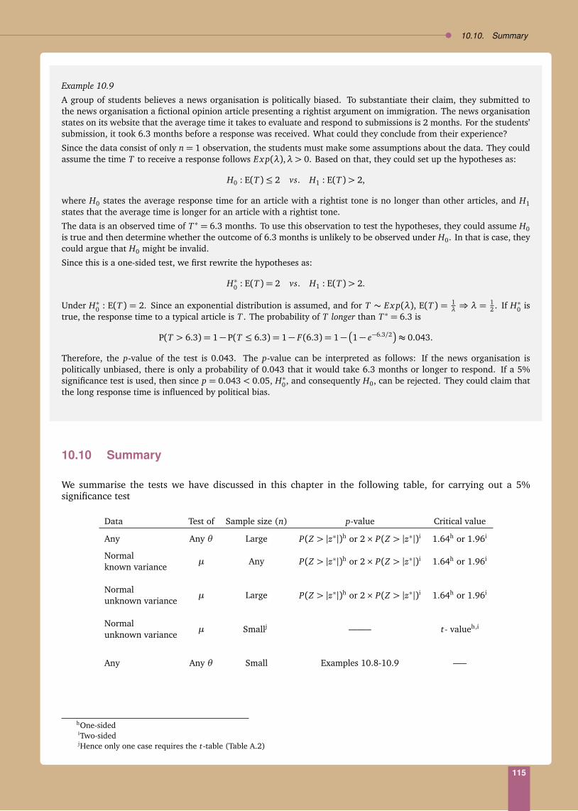
10.10. Summary
Example 10.9
A group of students believes a news organisation is politically biased. To substantiate their claim, they submitted tothe news organisation a fictional opinion article presenting a rightist argument on immigration. The news organisationstates on its website that the average time it takes to evaluate and respond to submissions is 2 months. For the students’submission, it took 6.3 months before a response was received. What could they conclude from their experience?
Since the data consist of only n= 1 observation, the students must make some assumptions about the data. They couldassume the time T to receive a response follows Ex p(λ),λ > 0. Based on that, they could set up the hypotheses as:
H0 : E(T )≤ 2 vs. H1 : E(T )> 2,
where H0 states the average response time for an article with a rightist tone is no longer than other articles, and H1states that the average time is longer for an article with a rightist tone.
The data is an observed time of T ∗ = 6.3 months. To use this observation to test the hypotheses, they could assume H0is true and then determine whether the outcome of 6.3 months is unlikely to be observed under H0. In that is case, theycould argue that H0 might be invalid.
Since this is a one-sided test, we first rewrite the hypotheses as:
H∗0 : E(T ) = 2 vs. H1 : E(T )> 2.
Under H∗0 : E(T ) = 2. Since an exponential distribution is assumed, and for T ∼ Ex p(λ), E(T ) = 1λ ⇒ λ =
12 . If H∗0 is
true, the response time to a typical article is T . The probability of T longer than T ∗ = 6.3 is
P(T > 6.3) = 1− P(T ≤ 6.3) = 1− F(6.3) = 1−
1− e−6.3/2
≈ 0.043.
Therefore, the p-value of the test is 0.043. The p-value can be interpreted as follows: If the news organisation ispolitically unbiased, there is only a probability of 0.043 that it would take 6.3 months or longer to respond. If a 5%significance test is used, then since p = 0.043 < 0.05, H∗0, and consequently H0, can be rejected. They could claim thatthe long response time is influenced by political bias.
10.10 Summary
We summarise the tests we have discussed in this chapter in the following table, for carrying out a 5%significance test
Data Test of Sample size (n) p-value Critical value
Any Any θ Large P(Z > |z∗|)h or 2× P(Z > |z∗|)i 1.64h or 1.96i
Normalµ Any P(Z > |z∗|)h or 2× P(Z > |z∗|)i 1.64h or 1.96i
known variance
Normalµ Large P(Z > |z∗|)h or 2× P(Z > |z∗|)i 1.64h or 1.96i
unknown variance
Normalµ Smallj ——– t- valueh,i
unknown variance
Any Any θ Small Examples 10.8-10.9 —–
hOne-sidediTwo-sidedjHence only one case requires the t-table (Table A.2)
115

11Association between Quantitative Variables
Is better schooling associated with higher economic growth? Does years of schooling have a relationship withcognitive skills? We are often interested in describing the association between two or more variables. In thischapter, we study methods for problems like these, when there are two variables and when both variables arequantitative. Many of the concepts we learn here generalise to more complex situations when there are morethan two variables and when variables can be both qualitative and quantitative.
We use data from E. Hanushek and L. Woessmann (2012),a who collected data on schooling, cognitiveskills and economic growth in 50 countries. To illustrate the methods discussed in this chapter, we only usea subset of the variables in the Hanushek-Woessmann data. The variables we use are the following: GDPgrowthb, Congitive skillsc, yrs. schoolingd, literacy sharee, OECDf.
Table 11.1: Cross country data for growth model
CODE Country GDP growthg Cognitive skillsg yrs schoolingg literacy shareg OECDh
1 ARG Argentina -1.5888 -0.8108 -1.6197 -0.3317 02 AUS Australia 0.0603 0.1157 0.7271 0.0314 13 AUT Austria 0.3742 0.3608 1.0349 0.1084 14 BEL Belgium 0.3035 0.2824 0.0659 0.0984 15 BRA Brazil -0.4624 -0.7098 -0.6186 -0.3554 06 CAN Canada 0.218 0.0752 0.4833 0.0466 17 CHE Switzerland -0.1473 -0.163 -1.3764 -0.0989 18 CHL Chile -0.6428 -0.4071 1.3285 -0.1061 09 CHN China 0.867 0.7233 -0.7916 0.2852 0
10 COL Colombia -1.3212 -0.2052 -0.5654 -0.0534 011 CYP Cyprus 1.5044 0.1434 0.904 0.1135 012 DNK Denmark 0.136 -0.0387 -0.2602 -0.027 113 EGY Egypt -0.7302 -0.2469 -1.4828 -0.0926 014 ESP Spain 0.4831 0.3055 0.399 0.1054 115 FIN Finland 0.3709 0.3922 0.4061 0.1332 116 FRA France 0.1258 0.2736 -0.3783 0.0907 117 GBR United Kingdom -0.1867 0.0439 0.9434 0.0461 1
aE. Hanushek and L. Woessmann (2012) Journal of Economic Growth, 17:267-231bGDP growth between 1960-2000. In our data, we adjusted the GDP growth figures by the 1960 GDP of each country, hence these
figures are different from those in the original Hanushek-Woessmann data. We use the same adjustment for all the other variables,except OECD. Since all variables are adjusted, they have sample mean zero
cScores on international tests on mathematics and sciencedAverage number of years of schooling between 1960-2000eShare of countries reaching basic literacyfWhether a country is a member of the Organisation for Economic Co-operation and Development, 1=“Yes", 0=“No"gAdjusted for 1960 GDPhOrganisation for Economic Co-operation and Development member countries
116

11.1. Scatter plot
18 GHA Ghana -2.2375 -0.6246 -1.4112 -0.2508 019 GRC Greece 0.1804 0.1251 0.9831 0.0581 120 HKG Hong Kong 2.416 0.7976 2.1231 0.2329 021 IDN Indonesia -0.0526 -0.3574 -0.6368 -0.1897 022 IND India -0.7027 0.0535 -2.2363 0.2684 023 IRL Ireland 1.2644 0.4315 1.1556 0.1469 124 IRN Iran -1.1406 -0.1471 -3.0159 0.0273 025 ISL Iceland 0.3444 0.1503 -0.8211 0.0666 126 ISR Israel 0.0637 0.1115 2.0329 0.0554 027 ITA Italy 0.2866 0.0712 -0.4228 0.0669 128 JOR Jordan -1.9413 -0.0767 0.5776 -0.0296 029 JPN Japan 1.3084 0.7897 3.8151 0.2142 130 KOR Korea, Rep. 2.5974 1.0535 3.2405 0.2891 131 MAR Morocco -0.7696 -0.9378 -3.1765 -0.3218 032 MEX Mexico -1.0387 -0.4706 -0.8601 -0.2454 133 MYS Malaysia 0.6247 0.5102 0.5043 0.1764 034 NLD Netherlands 0.1048 0.2409 -0.0914 0.0935 135 NOR Norway 0.5431 0.0347 1.4385 0.049 136 NZL New Zealand -0.8055 -0.0713 -0.7377 -0.0216 137 PER Peru -2.1846 -1.2778 -0.034 -0.5309 038 PHL Philippines -1.9718 -0.6717 0.51 -0.1994 039 PRT Portugal 0.8053 0.1367 -1.2963 0.0819 140 ROM Romania 0.161 0.3183 3.5007 0.1216 041 SGP Singapore 3.6084 0.9919 1.1693 0.2544 042 SWE Sweden -0.0767 0.0739 -0.2272 0.0455 143 THA Thailand 1.2148 0.3151 -0.0997 0.1903 044 TUN Tunisia -0.1181 -0.5165 -2.996 -0.2242 045 TUR Turkey -0.856 -0.2427 -1.8865 -0.1194 046 TWN Taiwan 3.2968 1.1755 1.9604 0.2885 047 URY Uruguay -1.5369 -0.3115 -1.0865 -0.168 048 USA United States 0.5783 -0.213 -0.3734 -0.0353 149 ZAF South Africa -1.8382 -1.4514 -1.5473 -0.4059 050 ZWE Zimbabwe -1.4918 -0.1457 0.7463 0.0216 0
In this chapter, we consider three approaches to study the association between two variables, they are:
(1) a graphical summary – scatter plot
(2) a numerical summary – correlation coefficient
(3) a model – regression analysis
11.1 Scatter plot
A scatter plot between cognitive skills and GDP growth is given in Fig. 11.1. In the scatter plot, there are 50symbols, one for each country in the dataset. Each symbol is given by the code of the country. Each symbolrepresents a pair of values for that country, one value for cognitive skills and one for GDP growth. We observefrom the scatter plot that those countries with higher value for cognitive skills tend to have higher GDP growth.Thus, the scatter plot suggests that the two variables may be positively associated or positively related. Insome cases, when a scatter plot shows that higher values of a variable tend to be paired with lower values ofanother variable, then we call the two variables negatively associated or negatively related. When we studyassociations or relationships between variables, we need to be careful on what the terms mean. When twovariables are related or associated, it does not mean that one causes another or one leads to another. Theyjust mean the two variables tend to vary in some systematic pattern.
We observe from Fig. 11.1 that the symbols seem to scatter around along a straight line trend, such arelationship is called a linear relationship and the two variables are said to be linearly related. In some
117

Chapter 11. Association between Quantitative Variables
Figure 11.1: Scatter plot of cognitive skills and GDP growth
−1.5 −0.5 0.0 0.5 1.0 1.5
−2
−1
01
23
4
Cognitive skills
GD
P g
row
th
ARG
AUS
AUTBEL
BRA
CAN
CHE
CHL
CHN
COL
CYP
DNK
EGY
ESPFIN
FRA
GBR
GHA
GRC
HKG
IDN
IND
IRL
IRN
ISL
ISRITA
JOR
JPN
KOR
MAR
MEX
MYS
NLD
NOR
NZL
PERPHL
PRT
ROM
SGP
SWE
THA
TUN
TUR
TWN
URY
USA
ZAF
ZWE
cases, a scatter plot shows symbols that seem to follow a curve, in such cases, the variables are non-linearlyrelated, see Fig 11.2(a)-(b). A scatter plot is useful for giving an overall impression of the kind of relationshipbetween the variables, e.g., linear or non-linear relationship. A scatter plot also allows us to identify unusualobservations. For example, in Fig 11.2(c), the scatter plot shows quickly that there is an unusual observationin the bottom left hand corner, +-mark, when it is compared to the trend of the other observations, whichshows higher values of one variable tend to be associated with lower values of the other variable; whereasfor that observation, the value of both variables are low. Unusual observations like that are called outliers.Normally, outliers must be treated with special care. The topic of outliers is beyond the scope here; we willnot pursue it further.
0 1 2 3 4
05
1015
(a) linear
0.0 0.4 0.8 1.2
02
46
810
(b) nonlinear
0 1 2 3 4
−8
−4
02
4
(c) outlier
Figure 11.2: Scatter plots showing linearly related variables, non-linearly related variables, and outliers
118

11.2. Correlation
11.2 Correlation
In Chapter 11.1, we showed that a simple graphical summary of the association of two variables is a scatterplot. Here, we study a simple numerical summary of of the association between two variables, when they arelinearly related.
Recall from Chapter 5.4, we defined a quantity called the covariance between two variables X and Y . Thecovariance between X , Y is given by Cov(X , Y ) = E[(X − µX )(Y − µY )], where µX ,µY stand for, respectively,the population means of X and Y ; Cov(X , Y ) > 0 when X and Y tend to agree, otherwise, Cov(X , Y ) < 0.Furthermore, Cov(X , Y ) is zero when X , Y are independent. Hence, we can consider Cov(X , Y ) as a measureof association between X and Y .
If we have n observations (X1, Y1),..., (Xn, Yn) measured on X and Y . Then the sample covariance isdefined by
sX Yg =
n∑
i=1
(X i − X )(Yi − Y )n− 1
= hn∑
i=1
X iYi − nX Yn− 1
A typical term in the numerator of the summation is (X i − X )(Yi − Y ) and it has the following characteristics.If X i and Yi both fall on the same side of their respective means, i.e.,
X i > X and Yi > Y or X i < X and Yi < Y
then this term is positive. If X i and Yi fall on opposite sides of their respective means, i.e.,
X i > X and Yi < Y or X i < X and Yi > Y
then this term is negative. If X and Y are two variables that are positively related, then they tend to takerelatively large values at the same time, and relatively low values at the same time. Hence, in a randomsample of (X , Y ) that are positively related, the sample covariance will likely be positive. On the contrary, if Xand Y are negatively related, then when one is relatively large, the other will be relatively small and a randomsample of (X , Y ) will have a negative sample covariance. We illustrate this concept using the growth data.
Example 11.1We use X and Y to denote cognitive skills and GDP growth, respectively. Both variables have sample means of zerosince we adjusted the data by 1960 GDP. We redraw the scatter plot, replacing country codes by +-marks. We use green+-marks to represent countries with values of both X and Y above their means, i.e., zero and red +-marks to representcountries such that one variable is above and the other variable is below zero, see Fig. 11.3. We observe that, except forfive countries, the rest are green +-marks. The green marks contribute positively to the sample covariance, while thered marks contribute negatively to the sample covariance. If we sum up the green and red marks, the result is:
sX Y =n∑
i=1
X iYi − nX Yn− 1
≈ (−0.8108)(−1.5888) + (0.1157)(0.0603) + ...+ (−0.1457)(−1.4918)− 50(0.01084588)(0.02597693)≈ 0.5927112(> 0),
which suggests higher cognitive skills are often associated with higher GDP growth in these countries.
gAnother version is∑n
i=1(X i−X )(Yi−Y )
n
hn∑
i=1
(X i − X )(Yi − Y ) =n∑
i=1
(X i Yi − X i Y − Yi X + X Y )
=n∑
i=1
X i Yi − Yn∑
i=1
X i − Xn∑
i=1
Yi +n∑
i=1
X Y
=n∑
i=1
X i Yi − nY X − nX Y + nX Y
=n∑
i=1
X i Yi − nX Y ⇒n∑
i=1
(X i − X )(Yi − Y )n− 1
=n∑
i=1
X i Yi − nX Yn− 1
119

Chapter 11. Association between Quantitative Variables
Figure 11.3: Scatter plot of cognitive skills and GDP growth relative to their means
−1.5 −1.0 −0.5 0.0 0.5 1.0 1.5
−3
−2
−1
01
23
4
X
Y
X
Y
Unfortunately, the covariance depends on the scale on which X and Y are measured. For example, ifcognitive skills score were increased by a factor of 10 for all countries, so that Argentina would have −8.108,Australia would have 1.157, etc.. That change does not change the relationship between cognitive skills andGDP growth. However, in that case, sX Y becomes 5.927112. Hence, the sign of sX Y can be used to determinewhether two variables are positively or negatively associated, but the magnitude of sX Y cannot be used to tellthe strength of the association.
If we divide Cov(X , Y ) by the standard deviations of X and Y , we obtain the correlation coefficienti
between X and Y ,
Corr(X , Y ) =Cov(X , Y )
SD(X )SD(Y )=
E(X −µX )(Y −µY )σXσY
= E
X −µX
σX
Y −µY
σY
= E︸︷︷︸
average
(zX zY )
where zX , zY are the z-scores of X and Y . Recall from Chapter 6 a positive z means a value is aboveits population mean, and negative if it is below its population mean. Hence, Corr(X , Y ) measures, onaverage, whether X and Y are in tandem relative to their population means. If X and Y are often intandem, Corr(X , Y ) > 0, otherwise, if X and Y are often on opposite sides of their respective means,then Corr(X , Y ) < 0. If Corr(X , Y ) = 0, then X and Y are not linearly related. It can be shownj that|Corr(X , Y )| ≤ 1. Furthermore, recall z-score also measures how far a value is from its population mean,hence if |Corr(X , Y )|= |E(zX zY )| is large (close to 1), then X and Y are often both far away from their meansat the same time, indicating a strong association. In this way, Corr(X , Y ) tells us both the direction and thestrength of the association between X and Y .
Based on a sample of n pairs of (X , Y ), we find a sample version of Corr(X , Y ), called a sample correlation
iThe correlation coefficient we discuss here is called a Pearson (product moment) correlation coefficient, after Egon SharpPearson, 1895-1980
jProof outside the scope of this course
120
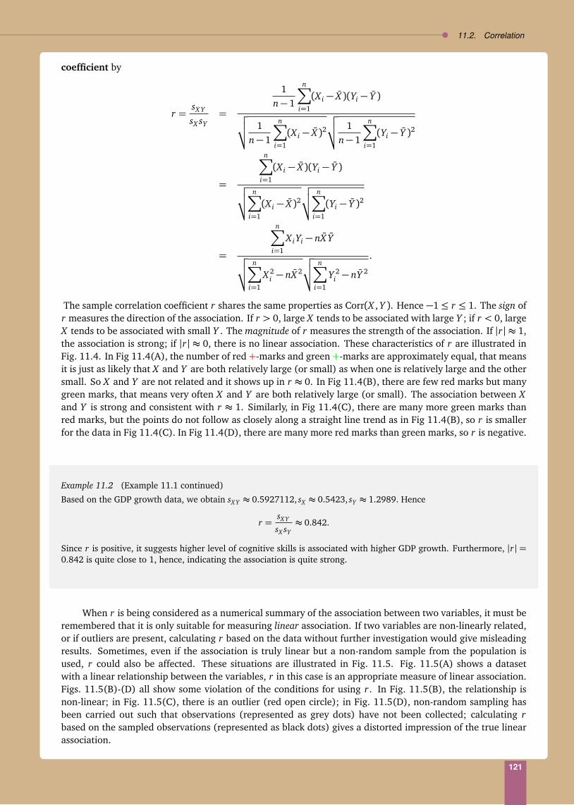
11.2. Correlation
coefficient by
r =sX Y
sX sY=
1n− 1
n∑
i=1
(X i − X )(Yi − Y )
√
√
√1
n− 1
n∑
i=1
(X i − X )2√
√
√1
n− 1
n∑
i=1
(Yi − Y )2
=
n∑
i=1
(X i − X )(Yi − Y )
√
√
√
n∑
i=1
(X i − X )2√
√
√
n∑
i=1
(Yi − Y )2
=
n∑
i=1
X iYi − nX Y
√
√
√
n∑
i=1
X 2i − nX 2
√
√
√
n∑
i=1
Y 2i − nY 2
.
The sample correlation coefficient r shares the same properties as Corr(X , Y ). Hence −1≤ r ≤ 1. The sign ofr measures the direction of the association. If r > 0, large X tends to be associated with large Y ; if r < 0, largeX tends to be associated with small Y . The magnitude of r measures the strength of the association. If |r| ≈ 1,the association is strong; if |r| ≈ 0, there is no linear association. These characteristics of r are illustrated inFig. 11.4. In Fig 11.4(A), the number of red +-marks and green +-marks are approximately equal, that meansit is just as likely that X and Y are both relatively large (or small) as when one is relatively large and the othersmall. So X and Y are not related and it shows up in r ≈ 0. In Fig 11.4(B), there are few red marks but manygreen marks, that means very often X and Y are both relatively large (or small). The association between Xand Y is strong and consistent with r ≈ 1. Similarly, in Fig 11.4(C), there are many more green marks thanred marks, but the points do not follow as closely along a straight line trend as in Fig 11.4(B), so r is smallerfor the data in Fig 11.4(C). In Fig 11.4(D), there are many more red marks than green marks, so r is negative.
Example 11.2 (Example 11.1 continued)
Based on the GDP growth data, we obtain sX Y ≈ 0.5927112, sX ≈ 0.5423, sY ≈ 1.2989. Hence
r =sX Y
sX sY≈ 0.842.
Since r is positive, it suggests higher level of cognitive skills is associated with higher GDP growth. Furthermore, |r| =0.842 is quite close to 1, hence, indicating the association is quite strong.
When r is being considered as a numerical summary of the association between two variables, it must beremembered that it is only suitable for measuring linear association. If two variables are non-linearly related,or if outliers are present, calculating r based on the data without further investigation would give misleadingresults. Sometimes, even if the association is truly linear but a non-random sample from the population isused, r could also be affected. These situations are illustrated in Fig. 11.5. Fig. 11.5(A) shows a datasetwith a linear relationship between the variables, r in this case is an appropriate measure of linear association.Figs. 11.5(B)-(D) all show some violation of the conditions for using r. In Fig. 11.5(B), the relationship isnon-linear; in Fig. 11.5(C), there is an outlier (red open circle); in Fig. 11.5(D), non-random sampling hasbeen carried out such that observations (represented as grey dots) have not been collected; calculating rbased on the sampled observations (represented as black dots) gives a distorted impression of the true linearassociation.
121

Chapter 11. Association between Quantitative Variables
Figure 11.4: Scatter plots and r showing different types of asociations
0.0 0.4 0.8
−5
05
10
(A) r = −0.063
X
Y
0.0 0.4 0.8
−5
05
10
(C) r = 0.652
X
Y
0.0 0.4 0.8
−5
05
10
(B) r = 0.935
X
Y
0.0 0.4 0.8
−5
05
10(D) r = −0.439
X
Y
11.3 Simple linear regression
If in addition to summarising the linear association between cognitive skills and GDP growth, we wish to studythe way GDP growth changes as a function of cognitive skills, then a regression analysis can be carried out.A scatter plot of cognitive skills and GDP growth (Fig. 11.6) shows there seems to be a linear relationshipbetween cognitive skills and GDP growth.
A regression analysis aims to investigate whether a linear relationship holds between cognitive skillsand GDP growth. Specifically, we postulate a linear relationship between cognitive skills and GDP growth,represented by a straight line, as follows:
GDP growth= a+ b(cognitive skills),
where a is the intercept and b is the slope of the line. In standard regression analysis parlance, cognitive skillsis either referred to as independent variable, predictor variable or covariate; GDP growth is referred to asdependent variable ,a outcome variable or response variable. The type of regression analysis discussed inthis chapter is called a simple linear regression because there is only one covariate and we wish to study alinear relationship between the covariate and the outcome. If we denote the covariate and outcome by X and
aThe terms “dependent" and “independent" are misleading since the value of the dependent variable does not need to depend onthe value of the independent variable
122

11.3. Simple linear regression
Figure 11.5: Violations of the conditions of r
A
C
B
D
Y , respectively, then the line can be rewritten as:
Y = a+ bX .
The intercept a can be interpreted as the value of Y when X = 0. However, often a is not of interest or mayeven be meaningless, e.g., if X represents the height of a person and Y represents the weight, then no personhas a height (X ) of zero. The value of b represents the change in the value of Y for every unit difference inthe value of X . In a linear regression, b captures the linear relationship between X and Y . If b = 0, then Xand Y are not linearly related; if b > 0, X and Y have a positive linear relationship and; if b < 0, X and Y arenegatively linearly related.
The scatter plot in Fig. 11.6 shows the data do not fall on the straight line. In fact, there is no straightline relationship that fits all the data. To solve this problem, we assume
Y = a+ bX + e, e ∼ N(0,σ2), (11.1)
where e is considered a “random" error or deviation of individual Y values from the straight line relationshipa+ bX . We call (11.1) a linear regression model, and a, b are are called regression coefficients
We interpret the regression model as follows:
(1) a+ bX is the average value of Y for observations with a particular value of X
123

Chapter 11. Association between Quantitative Variables
Figure 11.6: Postulated straight line relationship between cognitive skills and GDP growth
−1.5 −0.5 0.0 0.5 1.0 1.5
−3
−2
−1
01
23
4
Cognitive skills
GD
P g
row
th
ARG
AUS
AUTBEL
BRA
CAN
CHE
CHL
CHN
COL
CYP
DNK
EGY
ESPFIN
FRA
GBR
GHA
GRC
HKG
IDN
IND
IRL
IRN
ISL
ISRITA
JOR
JPN
KOR
MAR
MEX
MYS
NLD
NOR
NZL
PERPHL
PRT
ROM
SGP
SWE
THA
TUN
TUR
TWN
URY
USA
ZAF
ZWE
(2) Each observation Y differs from the average by an amount e, and e ∼ N(0,σ2)
(3) For each known value of X , the values of Y ∼ N(a + bX ,σ2). Since a + bX is the average of Y for aparticular X , it can be written as
E(Y |X ) = a+ bX .
E(Y |X ) is called a conditional expectation of Y given X . A conditional expectation has the samemeaning as an expectation that we discussed in Chapter 5. For example, in the context of the GDPgrowth data here, E(Y |X ) means the average GDP growth for countries with cognitive skills X . In aregression analysis, we assume we have known values of X at X1, ..., Xn and we investigate how E(Y |X )changes over these values, which is captured by the regression model
To investigate model (11.1), we need to find the unknowns a and b using the data. We will use maximumlikelihood estimation (MLE) from Chapter 8, which gives a solution equivalent to a method called ordinaryleast squares (OLS) in this setting.
11.3.1 Maximum likelihood and least squares solution
We have observations (X1, Y1), ..., (Xn, Yn). Using the model we postulate, Yi ∼ N(a+ bX i ,σ2), where a, b,σ2
are unknown, we can use the MLE to estimate these parameters. The log-likelihood is
`(a, b,σ2) = logn∏
i=1
1p
2πσ2exp
−Yi − (a+ bX i)2
2σ2
=n∑
i=1
−Yi − (a+ bX i)2
2σ2−
12
log2π− logσ
.
124

11.3. Simple linear regression
The MLEs a, b, and σ are obtained by taking derivative of `(a, b,σ2) with respect to a, b and σ and settingto zero:
d`(a, b, σ2)da
=n∑
i=1
Yi − (a+ bX i)= 0,
d`(a, b, σ2)d b
=n∑
i=1
Yi − (a+ bX i)X i = 0,
d`(a, b, σ2)dσ
=n∑
i=1
Yi − (a+ bX i)2
σ3−
nσ= 0,
solving for these three equations simultaneously, we obtain the MLE estimates of (a, b,σ2) as
b =
∑ni=1(X i − X )(Yi − Y )∑n
i=1(X i − X )2=
∑ni=1 X iYi − nX Y
∑ni=1 X 2
i − n(X )2=
sX Y
s2X
,
a = Y − bX , σ2 =1n
n∑
i=1
Yi − (a+ bX i)2. (11.2)
In the log-likelihood:
`(a, b,σ2) =n∑
i=1
−Yi − (a+ bX i)2
2σ2−
12
log2π− logσ
,
such that for any value of σ2, `(a, b,σ2) will be maximised if the sum of squares
n∑
i=1
Yi − (a+ bX i)2
is minimised, hence “least squares". This interpretation means that, MLE (least squares method) finds a linethat minimises the sum of squared deviations of the observations from the line. Hence in a sense, the MLEsolution gives the best “fitting" line to the data.
Example 11.3 (Example 11.1 continued)
Using the data from the 50 countries, we obtain the following summary statistics:
n∑
i=1
X i = −0.0002,n∑
i=1
Yi = −0.0003, sX Y ≈ 0.5927012, sX ≈ 0.5423, sY ≈ 1.2989.
b =0.5927012
0.54232≈ 2.0154, a = −0.0003/50− 2.0154(−0.0002/50)≈ 0.000002.
The quantities, a and b are estimates of the regression coefficients. To 4 decimal places, a = 0 due to the adjusted datavalues we used. In regression analyses of other dataset, a may take any value, depending on the relationship between thecovariate and the outcome. To four decimal places, the regression line estimated (sometimes we use the term “fitted")using data from the 50 countries is:
Y︸︷︷︸
GDP growth
= 2.0154× X︸︷︷︸
cognitive skills
, (11.3)
where we have used Y to denote estimated GDP growth from this estimated (fitted) linear regression model. A plot ofthe estimated regression model along with the scatter plot is given in Fig. 11.7.
125

Chapter 11. Association between Quantitative Variables
Figure 11.7: Fitted regression line: GDP growth = 2.0154×cognitive skills
−1.5 −0.5 0.0 0.5 1.0 1.5
−3
−2
−1
01
23
4
Cognitive skills
GD
P g
row
th
ARG
AUS
AUTBEL
BRA
CAN
CHE
CHL
CHN
COL
CYP
DNK
EGY
ESPFIN
FRA
GBR
GHA
GRC
HKG
IDN
IND
IRL
IRN
ISL
ISRITA
JOR
JPN
KOR
MAR
MEX
MYS
NLD
NOR
NZL
PERPHL
PRT
ROM
SGP
SWE
THA
TUN
TUR
TWN
URY
USA
ZAF
ZWE
11.3.2 Residual plot
Before we can use the estimated regression model for drawing inference, we must make inquiry about thequality of our model. First and foremost, we have made a number of assumptions in the model. In particular,we assumed there is an underlying straight line relationship, so that the data are randomly distributed aroundthe regression line, and data are equally likely to fall above or below the line. Furthermore, we assumed thatspread of the data from the line is constant over the observed range of the covariate. These two assumptionsimply the random error e = Y − (a+ bX ) to have mean zero and constant variance over the observed range ofX . Hence one way to determine whether the model assumptions have been violated is to study these randomerrors e. We estimate these random errors by residuals, defined by
ei = Yi − Yi
= Yi − (a+ bX i)
to answer the question and to assess the choice of a linear regression model for the data. If the modelassumptions are not violated, then the residuals eis should resemble a set of random observations with meanzero, and constant variance over the observed range of X . In other words, the residuals should display norecognisable patterns. If we plot the residuals on the vertical axis versus X is (Yis or Yis will also work) onthe horizontal axis, ideally, the plot should look like the top left hand panel of Fig. 11.8, where it can be seenthat the residuals show no relationship to the X -values. On the other hand, the remaining plots in Fig. 11.8reveal the data are of different degrees of departure from a simple linear model relationship. In particular, thetop right hand panel suggests the distribution of the error e is skewed; the residual plot shows a consistentlyhighly spread below zero than above zero, over the observed range of X . The bottom left hand panel indicatesthat the relationship between X and Y is non-linear; there is a clear non-linear trend in the residual plot. Thebottom right hand panel suggests the error distribution has non-constant variance across different values ofX ; the spread of the residuals changes over the observed range of X . When a residual plot suggests violationsof any of the assumptions in a regression model, then the data should be re-examined or a different modelshould be considered before proceeding. We will not pursue these topics further in this set of notes.
126

11.3. Simple linear regression
Figure 11.8: Examples of residual plots
0.0 0.4 0.8
−6
−2
02
46
Random
X
resi
dual
s
0
0.0 0.4 0.8
−6
−2
02
46
Non−linear
X
resi
dual
s
0
0.0 0.4 0.8
−6
−2
02
46
Skewed distribution
X
resi
dual
s
0
0.0 0.4 0.8
−6
−2
02
46
Non−constant varinace
X
resi
dual
s
0
127

Chapter 11. Association between Quantitative Variables
Figure 11.9: Residual plot for GDP growth data
X
resi
dual
s0
Example 11.4 (Example 11.1 continued)
Based on the regression modelY = 2.015× X ,
we can obtain ei , i = 1, ..., 50 by applying the regression model to the data. For example, for Argentina (ARG), X1 =−0.8108 so, to 4 decimal places,
Y1 = 2.0154× (−0.8108) = −1.6341,
which gives,e1 = Y1 − Y1 = −1.5888− (−1.6341) = 0.0453.
We use the same method to obtain the remaining residuals, which are given in the following table. The correspondingresidual plot, Fig. 11.9, is obtained by plotting (ei , X i), i = 1, ..., 50. By inspection, the residuals are consistent with aset of “random" errors, centred at zero; there is no evidence that the spread of the residuals changes over the observedrange of X . Therefore, we conclude there is no violation of the assumptions of a simple linear regression model.
Country code Yi Yi ei
ARG -1.5888 -1.6341 0.0453AUS 0.0603 0.2332 -0.1729AUT 0.3742 0.7272 -0.3530BEL 0.3035 0.5691 -0.2656BRA -0.4624 -1.4305 0.9681
......
......
URY -1.5369 -0.6278 -0.9091USA 0.5783 -0.4293 1.0076ZAF -1.8382 -2.9252 1.0870ZWE -1.4918 -0.2936 -1.1982
128

11.3. Simple linear regression
11.3.3 Hypothesis testing
The regression line (11.3) obtained in Example 11.3 gives an estimated model between GDP growth (Y ) andcognitive skills (X ) based on a sample of 50 countries. Naturally, the question arises that, can we generaliseour observation in this sample into a general model between GDP growth and cognitive skills? Before weanswer this question, it is important for us to realise that “countries" are no more than labels, they have nobearing on the results of our study. We view the data as n = 50 random observations of (X , Y ) and we querywhether the relationship observed in the data is an indication of an underlying relationship between X and Y .
A linear relationship between GDP growth and cognitive skills means that in model (11.1), b 6= 0. Noticethe difference between b in (11.1) and b in (11.3); b is in the estimated model and applies to the n = 50observations while b is in the model of a general underlying linear relationship.
To investigate whether an underlying linear relationship exists between GDP growth and cognitive skills,we can use the data to test the following hypotheses:
H0 : b = 0 vs. H1 : b 6= 0. (11.4)
We follow the methods in Chapter 10 to carry out the test. Recall from Chapter 10 that, we first assume H0 istrue, and then examine whether the observed data suggest otherwise. We can show b is just a combination ofYis,
k much like X is a combination of X is. Since in a regression model, we assume Yis are normally distributed,hence, we can use a test for normal data, similar to the tests in Chapter 10.8.
Since b is an MLE of b, then according to methods in Chapter 10.8, we can use the following test statistic
t∗ =b− 0cSE(b)
=b
σ/q
∑ni=1(X i − X )2
, (11.5)
where cSE(b)l is an estimate of SE(b) and σ can be the MLE of σ from (11.2).
We need to compare t∗ from our data to t from a typical sample of observations of (X , Y ) with nolinear relationship in X and Y . If t∗ is significantly different from a typical t, then our data suggest a linearrelationship in (X , Y ).
Often, we call t∗ significantly different from t if no more than 5% of the ts are as large as |t∗|. This isan example of a 5% significance test discussed in Chapter 10. A table of the critical t values for determiningwhether t∗ is significantly different from t is given in Table A.2.
kLet ci = (X i − X ), i = 1, ..., n and d =∑n
i=1(X i − X )2, which are constants since we assume in a regression model that X is areconstants. Hence
b =
∑ni=1(X i − X )(Yi − Y )∑n
i=1(X i − X )2=
n∑
i=1
ci(Yi − Y )d
,
which is just a linear combination of Yis.
lSince∑n
i=1(X i − X )(Yi − Y ) =∑n
i=1(X i − X )Yi −∑n
i=1(X i − X )Y =∑n
i=1(X i − X )Yi − Y
=0︷ ︸︸ ︷
n∑
i=1
(X i − X ), we can write
b =
∑ni=1(X i − X )(Yi − Y )∑n
i=1(X i − X )2=
∑ni=1(X i − X )Yi
∑ni=1(X i − X )2
Earlier, we learned
Var(b) =
∑ni=1(X i − X )2Var(Yi)∑n
i=1(X i − X )22 =
∑ni=1(X i − X )2σ2
∑ni=1(X i − X )2
2 =σ2
∑ni=1(X i − X )2
,
where in the above, we have made used of the fact that X1, ..., Xn are assumed known and hence X i − X are constants. Furthermore,σ can be replaced by an estimate σ. Finally
cSE(b) =q
ÓVar(b) =σ
q
∑ni=1(X i − X )2
.
129
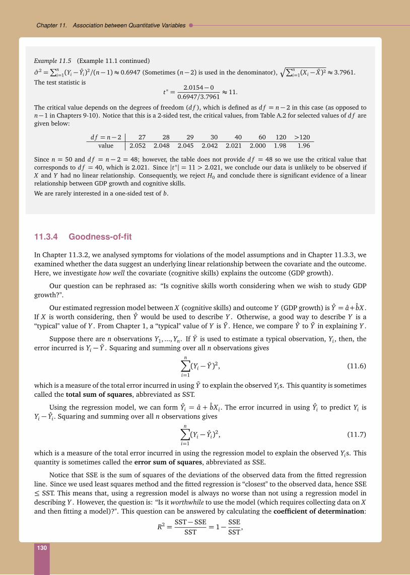
Chapter 11. Association between Quantitative Variables
Example 11.5 (Example 11.1 continued)
σ2 =∑n
i=1(Yi − Yi)2/(n− 1)≈ 0.6947 (Sometimes (n− 2) is used in the denominator),q
∑ni=1(X i − X )2 ≈ 3.7961.
The test statistic is
t∗ =2.0154− 0
0.6947/3.7961≈ 11.
The critical value depends on the degrees of freedom (d f ), which is defined as d f = n− 2 in this case (as opposed ton−1 in Chapters 9-10). Notice that this is a 2-sided test, the critical values, from Table A.2 for selected values of d f aregiven below:
d f = n− 2 27 28 29 30 40 60 120 >120value 2.052 2.048 2.045 2.042 2.021 2.000 1.98 1.96
Since n = 50 and d f = n − 2 = 48; however, the table does not provide d f = 48 so we use the critical value thatcorresponds to d f = 40, which is 2.021. Since |t∗| = 11 > 2.021, we conclude our data is unlikely to be observed ifX and Y had no linear relationship. Consequently, we reject H0 and conclude there is significant evidence of a linearrelationship between GDP growth and cognitive skills.
We are rarely interested in a one-sided test of b.
11.3.4 Goodness-of-fit
In Chapter 11.3.2, we analysed symptoms for violations of the model assumptions and in Chapter 11.3.3, weexamined whether the data suggest an underlying linear relationship between the covariate and the outcome.Here, we investigate how well the covariate (cognitive skills) explains the outcome (GDP growth).
Our question can be rephrased as: “Is cognitive skills worth considering when we wish to study GDPgrowth?".
Our estimated regression model between X (cognitive skills) and outcome Y (GDP growth) is Y = a+ bX .If X is worth considering, then Y would be used to describe Y . Otherwise, a good way to describe Y is a“typical" value of Y . From Chapter 1, a “typical" value of Y is Y . Hence, we compare Y to Y in explaining Y .
Suppose there are n observations Y1, ..., Yn. If Y is used to estimate a typical observation, Yi , then, theerror incurred is Yi − Y . Squaring and summing over all n observations gives
n∑
i=1
(Yi − Y )2, (11.6)
which is a measure of the total error incurred in using Y to explain the observed Yis. This quantity is sometimescalled the total sum of squares, abbreviated as SST.
Using the regression model, we can form Yi = a + bX i . The error incurred in using Yi to predict Yi isYi − Yi . Squaring and summing over all n observations gives
n∑
i=1
(Yi − Yi)2, (11.7)
which is a measure of the total error incurred in using the regression model to explain the observed Yis. Thisquantity is sometimes called the error sum of squares, abbreviated as SSE.
Notice that SSE is the sum of squares of the deviations of the observed data from the fitted regressionline. Since we used least squares method and the fitted regression is “closest" to the observed data, hence SSE≤ SST. This means that, using a regression model is always no worse than not using a regression model indescribing Y . However, the question is: “Is it worthwhile to use the model (which requires collecting data on Xand then fitting a model)?". This question can be answered by calculating the coefficient of determination:
R2 =SST− SSE
SST= 1−
SSESST
,
130

11.3. Simple linear regression
which is a function of (11.6) and (11.7). The value of R2 (pronounced “R-square") is between 0 and 1. R2 canbe interpreted as the proportion of prediction error reduction using a model compared to not using a model.The quantity SST−SSE= SSR is called a regression sum of squares. A large value of R2 indicates the modelexplains Y , or it provides a “good fit".m
The quantity SST is also called the total variation of the data because it measures the overall variationbetween individual observations and the mean Y . The quantity SSR is also called the explained variationby X because it captures the “reduction" in variation that resulted from using X to predict Yi by fitting asimple linear regression. The quantity SSE is also called the unexplained variation because it represents theremaining errors in using Yi for predicting Yi even after fitting the regression; hence the errors that cannot beexplained by knowing X .
In the case of a simple linear regression, R2 has the following simple relationship to the sample correlationcoefficient, r:
R2 = r2, (11.8)
so if r is already calculated using one of the formulae in Chapter 11.2, then we can determine R2 easily using(11.8). When there is more than one covariate, R2 replaces r as a single number summary of the associationbetween the outcome and all its covariates (e.g., cognitive skills, yrs. schooling, literacy share, etc.). Note thatunlike r, which ranges from −1 to 1, R2 ranges from 0 to 1. This difference between r and R2 is not surprising.In the case of r, we are measuring the association between one outcome and one covariate; hence it makessense to talk about positive and negative associations, which are captured by the sign of r. In the case ofR2, we may be measuring the association between one outcome and more than one covariate, some of themmay have a positive association with the outcome and some of them may have a negative association with theoutcome; hence it is not possible to have a single number summary of the direction of association between theoutcome and all its the covariates. However, we can still talk about the strength of the association betweenthe outcome and its covariate(s) using R2.
If we multiply R2 × 100 percent, we obtain the percent variation explained, which is another way ofexpressing the usefulness of the regression model. The higher the percent variation explained, the more usefulis a regression model.
Example 11.6
In Example 11.1, the correlation coefficient between GDP growth and cognitive skills is 0.842, then the coefficient ofdetermination is 0.8422 = 0.709. In this case, percent variation explained = 0.709× 100≈ 70%. We usually expressedsuch result by writing “approximately 70% of the variation in GDP growth is explained by cognitive skills". This statementmeans 70% of differences in GDP growth between countries is explained by cognitive skills, while 30%, of the differencesin GDP growth between countries are due to other unknown factors.
11.3.5 Prediction using a regression model
The main goals of a regression analysis are to determine if a relationship exists between an outcome and itscovariate and if there is, to explain the outcome using the covariate. Based on the fitted regression model,we can obtain estimates of b and Y using b and Y . In the context of the GDP growth data, b represents ourestimate of the change in GDP growth for a unit change in cognitive skills, while Y represents the predicted(average) GDP growth for countries with cognitive skills at level X . However, since both b and Y are estimatedbased on a sample of observations of (X , Y ), they are subject to sampling errors, as discussed in Chapters 8-9.To allow for sampling errors in our estimates, we consider interval estimates here.
mEven though there is no universal benchmark of what value of R2 constitutes a good fit, a commonly accepted guideline is: <0.1(poor), 0.1−0.3 (weak), 0.3−0.5 (moderate), 0.5−0.7 (good), >0.7 (very good), Cohen, 1988, Statistical power analysis for thebehavioral sciences (2nd ed.), Hillsdale, NJ: Lawrence Earlbaum Associates.
131
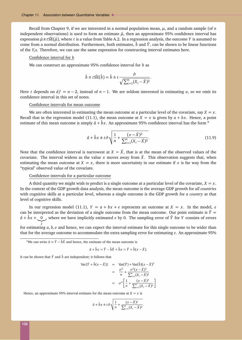
Chapter 11. Association between Quantitative Variables
Recall from Chapter 9, if we are interested in a normal population mean, µ, and a random sample (of nindependent observations) is used to form an estimate µ, then an approximate 95% confidence interval hasexpression µ± tSE(µ), where t is a value from Table A.2. In a regression analysis, the outcome Y is assumed tocome from a normal distribution. Furthermore, both estimates, b and Y , can be shown to be linear functionsof the Yis. Therefore, we can use the same expression for constructing interval estimates here.
Confidence interval for b
We can construct an approximate 95% confidence interval for b as
b± tSE(b) = b± tσ
q
∑ni=1(X i − X )2
.
Here t depends on d f = n − 2, instead of n − 1. We are seldom interested in estimating a, so we omit itsconfidence interval in this set of notes.
Confidence intervals for mean outcome
We are often interested in estimating the mean outcome at a particular level of the covariate, say X = x .Recall that in the regression model (11.1), the mean outcome at X = x is given by a + bx . Hence, a pointestimate of this mean outcome is simply a+ bx . An approximate 95% confidence interval has the form n
a+ bx ± tσ
√
√
√1n+
(x − X )2∑n
i=1(X i − X )2. (11.9)
Note that the confidence interval is narrowest at X = X , that is at the mean of the observed values of thecovariate. The interval widens as the value x moves away from X . This observation suggests that, whenestimating the mean outcome at X = x , there is more uncertainty in our estimate if x is far way from the“typical" observed value of the covariate.
Confidence intervals for a particular outcome
A third quantity we might wish to predict is a single outcome at a particular level of the covariate, X = x .In the context of the GDP growth data analysis, the mean outcome is the average GDP growth for all countrieswith cognitive skills at a particular level, whereas a single outcome is the GDP growth for a country at thatlevel of cognitive skills.
In our regression model (11.1), Y = a + bx + e represents an outcome at X = x . In the model, ecan be interpreted as the deviation of a single outcome from the mean outcome. Our point estimate is Y =a + bx + 0
︸︷︷︸
e
, where we have implicitly estimated e by 0. The sampling error of Y for Y consists of errors
for estimating a, b, e and hence, we can expect the interval estimate for this single outcome to be wider thanthat for the average outcome to accommodate the extra sampling error for estimating e. An approximate 95%
nWe can write a = Y − bX and hence, the estimate of the mean outcome is
a+ bx = Y − bX + bx = Y + b(x − X ).
It can be shown that Y and b are independent; it follows that
VarY + b(x − X ) = Var(Y ) + Var(b)(x − X )2
=σ2
n+
σ2(x − X )2∑n
i=1(X i − X )2
= σ2
1n+
(x − X )2∑n
i=1(X i − X )2
Hence, an approximate 95% interval estimate for the mean outcome at X = x is
a+ bx ± tσ
√
√
√1n+
(x − X )2∑n
i=1(X i − X )2.
132

11.3. Simple linear regression
confidence interval is: o
a+ bx ± tσ
√
√
√
1+1n+
(x − X )2∑n
i=1(X i − X )2. (11.10)
We call (11.10) a prediction interval to distinguish it from (11.9), which is for the mean outcome.
Comparing (11.9) and (11.10), we notice the prediction interval looks very similar to the confidenceinterval, except there is an extra “1" in the prediction interval. This means the prediction interval is alwayswider than the corresponding confidence interval, for the same data set and X = x . This result is reasonablesince we would expect more uncertainty due to the extra sampling error in estimating e.
Whether we are predicting the mean outcome, or a single outcome, a regression model only allowsprediction be made within the observed range of the covariate X . For the GDP growth data, for example,since the lowest and the highest cognitive skills in the 50 countries are −1.4514 (South Africa) and 1.1755(Taiwan), therefore, prediction on GDP growth can only be made for countries with cognitive skills within thisrange. For countries with cognitive skills outside (−1.4514, 1.1755), no prediction is possible. This restrictiondoes not apply to the outcome variable. In other words, using the regression model, the predicted GDP growthcan be outside the range of Y values observed in the 50 countries.
Example 11.7 (Example 11.1 continued)For the data from the 50 countries, we can determine a 95% interval for b. We need to estimate σ2 using (11.2):σ2 =
∑ni=1Yi − (a+ bX i)2/n. Notice that Yi − (a+ bX i) is the residual ei that we defined earlier. From Example 11.4,
we obtain σ ≈ 0.6947. Furthermore∑n
i=1(X i − X )2 = 14.41033, X = −0.0002/50 = −0.00004. From Example 11.5,we use a value of t = 2.000 from Table A.2.Hence, an approximate 95% confidence interval for b is
b± 2.000σ
q
∑ni=1(X i − X )2
= 2.0154± 2.0000.69473.7961
≈ (1.6493, 2.3814).
Suppose next we are interested in estimating the mean GDP growth for countries with cognitive skills of 0.5. Then apoint estimate of the mean GDP growth in that group of countries is
a+ b(0.5) = 2.0154× 0.5≈ 1.0077
and an approximate 95% confidence interval is
a+bx±2.000σ
√
√
√1n+
(x − X )2∑n
i=1(X i − X )2= 0+2.0154(0.5)±2.000(0.6947)
√
√ 150+[0.5− (−0.00004)]2
14.41033≈ (0.7391, 1.2762).
If however, we are simply interested in estimating GDP growth for a country with cognitive skills of 0.5, then we use theprediction interval and an approximate 95% prediction interval for GDP growth is
a+ bx ± 2.000σ
√
√
√
1+1n+
(x − X )2∑n
i=1(X i − X )2= 0+ 2.0154(0.5)± 2.000(0.6947)
√
√
1+150+[0.5− (−0.00004)]2
14.41033
≈ (−0.4074, 2.4228).
o
Var(Y ) = Var(a+ bX ) + Var(e)
= σ2
1n+
(x − X )2∑n
i=1(X i − X )2
+σ2
= σ2
1+1n+
(x − X )2∑n
i=1(X i − X )2
.
Hence, an approximate 95% interval estimate for a particular outcome Y at X = x is
a+ bx ± tσ
√
√
√
1+1n+
(x − X )2∑n
i=1(X i − X )2.
133

Chapter 11. Association between Quantitative Variables
Figure 11.10: Confidence and prediction bands for GDP growth data
−1.5 −0.5 0.0 0.5 1.0 1.5
−2
02
4
Cognitive skills
GD
P g
row
th
ARG
AUS
AUTBEL
BRA
CAN
CHE
CHL
CHN
COL
CYP
DNK
EGY
ESPFIN
FRA
GBR
GHA
GRC
HKG
IDN
IND
IRL
IRN
ISL
ISRITA
JOR
JPN
KOR
MAR
MEX
MYS
NLD
NOR
NZL
PERPHL
PRT
ROM
SGP
SWE
THA
TUN
TUR
TWN
URY
USA
ZAF
ZWE
PredictionConfidence
Comparing the two intervals, we find the prediction interval considerably wider. This result means that the prediction ofone country’s outcome is less precise than the prediction of the mean outcome of a group of countries of similar cognitiveskills.
In fact, we can use (11.9) and (11.10) to create 95% confidence and prediction bands across different values of X . Thisprocess can be done using a computer. The results for the GDP growth data are given in Fig. 11.10. The bands areuseful for reading off 95% confidence and prediction intervals at different values of X . As an illustration, a gray verticalline at X = 0.5 is drawn, the points of intersection of that line with the bands give the ends of the 95% confidence andprediction intervals at X = 0.5.
134

AStatistical Tables
0 z*
135

Table A.1: Areas under the standard normal curve beyond z∗, i.e., shaded area
z∗ 0.00 0.01 0.02 0.03 0.04 0.05 0.06 0.07 0.08 0.09
0.0 0.5000 0.4960 0.4920 0.4880 0.4840 0.4801 0.4761 0.4721 0.4681 0.46410.1 0.4602 0.4562 0.4522 0.4483 0.4443 0.4404 0.4364 0.4325 0.4286 0.42470.2 0.4207 0.4168 0.4129 0.4090 0.4052 0.4013 0.3974 0.3936 0.3897 0.38590.3 0.3821 0.3783 0.3745 0.3707 0.3669 0.3632 0.3594 0.3557 0.3520 0.34830.4 0.3446 0.3409 0.3372 0.3336 0.3300 0.3264 0.3228 0.3192 0.3156 0.31210.5 0.3085 0.3050 0.3015 0.2981 0.2946 0.2912 0.2877 0.2843 0.2810 0.27760.6 0.2743 0.2709 0.2676 0.2643 0.2611 0.2578 0.2546 0.2514 0.2483 0.24510.7 0.2420 0.2389 0.2358 0.2327 0.2296 0.2266 0.2236 0.2206 0.2177 0.21480.8 0.2119 0.2090 0.2061 0.2033 0.2005 0.1977 0.1949 0.1922 0.1894 0.18670.9 0.1841 0.1814 0.1788 0.1762 0.1736 0.1711 0.1685 0.1660 0.1635 0.16111.0 0.1587 0.1562 0.1539 0.1515 0.1492 0.1469 0.1446 0.1423 0.1401 0.13791.1 0.1357 0.1335 0.1314 0.1292 0.1271 0.1251 0.1230 0.1210 0.1190 0.11701.2 0.1151 0.1131 0.1112 0.1093 0.1075 0.1056 0.1038 0.1020 0.1003 0.09851.3 0.0968 0.0951 0.0934 0.0918 0.0901 0.0885 0.0869 0.0853 0.0838 0.08231.4 0.0808 0.0793 0.0778 0.0764 0.0749 0.0735 0.0721 0.0708 0.0694 0.06811.5 0.0668 0.0655 0.0643 0.0630 0.0618 0.0606 0.0594 0.0582 0.0571 0.05591.6 0.0548 0.0537 0.0526 0.0516 0.0505 0.0495 0.0485 0.0475 0.0465 0.04551.7 0.0446 0.0436 0.0427 0.0418 0.0409 0.0401 0.0392 0.0384 0.0375 0.03671.8 0.0359 0.0351 0.0344 0.0336 0.0329 0.0322 0.0314 0.0307 0.0301 0.02941.9 0.0287 0.0281 0.0274 0.0268 0.0262 0.0256 0.0250 0.0244 0.0239 0.02332.0 0.0228 0.0222 0.0217 0.0212 0.0207 0.0202 0.0197 0.0192 0.0188 0.01832.1 0.0179 0.0174 0.0170 0.0166 0.0162 0.0158 0.0154 0.0150 0.0146 0.01432.2 0.0139 0.0136 0.0132 0.0129 0.0125 0.0122 0.0119 0.0116 0.0113 0.01102.3 0.0107 0.0104 0.0102 0.0099 0.0096 0.0094 0.0091 0.0089 0.0087 0.00842.4 0.0082 0.0080 0.0078 0.0075 0.0073 0.0071 0.0069 0.0068 0.0066 0.00642.5 0.0062 0.0060 0.0059 0.0057 0.0055 0.0054 0.0052 0.0051 0.0049 0.00482.6 0.0047 0.0045 0.0044 0.0043 0.0041 0.0040 0.0039 0.0038 0.0037 0.00362.7 0.0035 0.0034 0.0033 0.0032 0.0031 0.0030 0.0029 0.0028 0.0027 0.00262.8 0.0026 0.0025 0.0024 0.0023 0.0023 0.0022 0.0021 0.0021 0.0020 0.00192.9 0.0019 0.0018 0.0018 0.0017 0.0016 0.0016 0.0015 0.0015 0.0014 0.00143.0 0.0013 0.0013 0.0013 0.0012 0.0012 0.0011 0.0011 0.0011 0.0010 0.0010
136
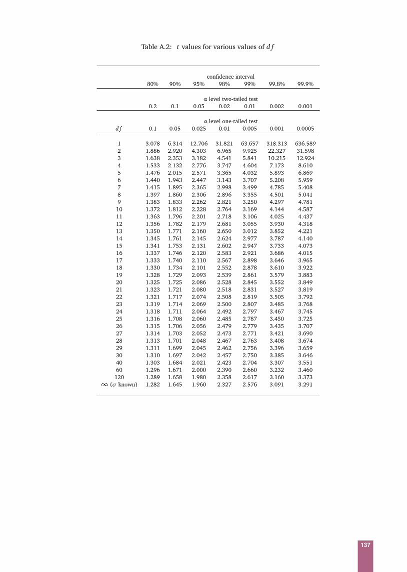
Table A.2: t values for various values of d f
confidence interval80% 90% 95% 98% 99% 99.8% 99.9%
α level two-tailed test0.2 0.1 0.05 0.02 0.01 0.002 0.001
α level one-tailed testd f 0.1 0.05 0.025 0.01 0.005 0.001 0.0005
1 3.078 6.314 12.706 31.821 63.657 318.313 636.5892 1.886 2.920 4.303 6.965 9.925 22.327 31.5983 1.638 2.353 3.182 4.541 5.841 10.215 12.9244 1.533 2.132 2.776 3.747 4.604 7.173 8.6105 1.476 2.015 2.571 3.365 4.032 5.893 6.8696 1.440 1.943 2.447 3.143 3.707 5.208 5.9597 1.415 1.895 2.365 2.998 3.499 4.785 5.4088 1.397 1.860 2.306 2.896 3.355 4.501 5.0419 1.383 1.833 2.262 2.821 3.250 4.297 4.781
10 1.372 1.812 2.228 2.764 3.169 4.144 4.58711 1.363 1.796 2.201 2.718 3.106 4.025 4.43712 1.356 1.782 2.179 2.681 3.055 3.930 4.31813 1.350 1.771 2.160 2.650 3.012 3.852 4.22114 1.345 1.761 2.145 2.624 2.977 3.787 4.14015 1.341 1.753 2.131 2.602 2.947 3.733 4.07316 1.337 1.746 2.120 2.583 2.921 3.686 4.01517 1.333 1.740 2.110 2.567 2.898 3.646 3.96518 1.330 1.734 2.101 2.552 2.878 3.610 3.92219 1.328 1.729 2.093 2.539 2.861 3.579 3.88320 1.325 1.725 2.086 2.528 2.845 3.552 3.84921 1.323 1.721 2.080 2.518 2.831 3.527 3.81922 1.321 1.717 2.074 2.508 2.819 3.505 3.79223 1.319 1.714 2.069 2.500 2.807 3.485 3.76824 1.318 1.711 2.064 2.492 2.797 3.467 3.74525 1.316 1.708 2.060 2.485 2.787 3.450 3.72526 1.315 1.706 2.056 2.479 2.779 3.435 3.70727 1.314 1.703 2.052 2.473 2.771 3.421 3.69028 1.313 1.701 2.048 2.467 2.763 3.408 3.67429 1.311 1.699 2.045 2.462 2.756 3.396 3.65930 1.310 1.697 2.042 2.457 2.750 3.385 3.64640 1.303 1.684 2.021 2.423 2.704 3.307 3.55160 1.296 1.671 2.000 2.390 2.660 3.232 3.460
120 1.289 1.658 1.980 2.358 2.617 3.160 3.373∞ (σ known) 1.282 1.645 1.960 2.327 2.576 3.091 3.291
137

BBasic Algebra and Calculus
B.1 Factorials
If n is a non-negative integer, then n! (called “n factorial") is defined by:
n!= 1× 2× 3× ...× n.
By convention, 0!= 1.
Example B.1
1! = 1
4! = 1× 2× 3× 4= 24
6! = 1× 2× 3× 4× 5× 6= 720
If n, m are non-negative integers such that n≥ m, then nCm (called “n choose m") is defined by:
nCm ≡
nm
=n!
(n−m)!m!.
Example B.2
6C2 =
62
=6!
(6− 2)!2!=
720(24)(2)
= 15
6C6 =
66
=6!
(6− 6)!6!=
720(1)(720)
= 1
138

B.2 Significant digits & decimal places
Significant digits or signficant figures refer to the number of figures in a number that would be meaningful,relative to its magnitude.
Example B.3
a. 4.3333 to 2 significant digits is 4.3.
b. 43.3333 to 2 significant digits is 43.
c. 433.3333 to 2 significant digits is 430.
d. 4333.3333 to 2 significant digits is 4300.
e. 0.0043333 to 2 significant digits is 0.0043.
f. 4.3333 to 2 decimal places is 4.33.
g. 43.3333 to 2 decimal places is 43.33.
h. 433.3333 to 2 decimal places is 433.33.
i. 4333.3333 to 2 decimal places is 4333.33.
j. 0.0043333 to 2 decimal places is 0.00.
Comparing the figures, it is very clear that rounding off a number by significant digits gives moreinterpretable results. In most statistical analyses, numbers usually can be rounded off to 3 significant digitswithout a cost to precision. However, if there is a problem that involves intermediate steps, then a few moresignificant digits should be preserved for the intermediate steps.
B.3 The summation sign Σ
Suppose the following set of data is obtained on a variable X :
1, 2, 3, 3, 6,
the observations can be denoted as X1, X2, ..., Xn, where n= 5. The sum is given by
5∑
i=1
X i = X1 + X2 + ...+ X5 = 1+ 2+ 3+ 3+ 6.
In general, the sum of n numbers X1, ..., Xn can be represented by the shorthand notation∑n
i=1 X i ,∑
i X i or∑
X i . The symbol∑
is the upper case Greek letter “sigma". This notation is especially useful when there aremany terms to sum up.
Example B.4∑
X i = X1 + X2 + X3 + X4 + X5 = 1+ 2+ 3+ 3+ 6
X ≡∑
X i
n=
X1 + X2 + X3 + X4 + X5
5=
1+ 2+ 3+ 3+ 65
∑
X 2i = X 2
1 + X 22 + X 2
3 + X 24 + X 2
5 = 1+ 4+ 9+ 9+ 36∑
X i
2= (X1 + X2 + X3 + X4 + X5)
2 = (1+ 2+ 3+ 3+ 6)2∑
(X i − X )2 = (X1 − X )2 + (X2 − X )2 + (X3 − X )2 + (X4 − X )2 + (X5 − X )2
= (1− 3)2 + (2− 3)2 + (3− 3)2 + (4− 3)2 + (6− 3)2
139

B.4 The product sign Π
Suppose the following set of data is obtained on a variable X :
1, 2, 3, 3, 6,
the observations can be denoted as X1, X2, ..., Xn, where n= 5. The product of these observations is
Π5i=1X i = X1 × X2 × ...× X5 = 1× 2× 3× 3× 6.
In general, a product of n numbers X1, ..., Xn can be represented by the shorthand notation Πni=1X i , ΠiX i or
simply ΠX i . The symbol Π is the upper case Greek letter “pi". This notation is especially useful when thereare many terms to multiply together.
B.5 Series
A sequence of numbers can be represented symbolically as X1, X2, ..., X i , .... A (infinite) series is defined asthe sum X1 + X2 + ...+ X i + ... or as
∑∞i=1 X i . Some special series are:
• Arithematic series – An arithematic series is a series where each successive term is produced by addingthe previous term by a constant number, e.g.,
1+ 2+ 3+ ...+ n+ ...
In general, an arithematic series can be written as:
∞∑
i=1
a+ i × b
where a, b are constants.
• Power series – A power series in x is a series that can be expressed as
∞∑
i=1
ai(x − b)i
where ai is a sequence of numbers and b is a constant, e.g.,
20
1!+
21
2!+
22
3!+ ...+
2n
n!+ ....
• Geometric series – A geometric series is a series where each successive term is produced by multiplyingthe previous term by a constant number, e.g.,
20 + 21 + 22 + ...+ 2n + ....
In general, a geometric series in a constant a is written as
∞∑
i=1
ai .
140

B.6 Functions
A generic notation for a function is g(x). For generic constants, a, b, c, d, some common functions are:
g(x) = a constant functiong(x) = a+ bx linear functiong(x) = a+ bx + cx2 quadratic functiong(x) = a+ bx + cx2 + d x3 cubic functiong(x) = eax exponential functiong(x) = logax logarithmic function
Logarithmic and exponential functions
In Statistics, we often use logarithm to the base e, or sometimes known as natural logarithm. In here,unless otherwise stated, all logarithms are natural logarithms. Some common properties of the logarithmicand exponential functions are:
logx = y ⇔ x = e y
logx y = logx + logylog x
y = logx − logylogxa = alogxlog1 = 0loge = 1
e0 = 1ex+y = ex e y
eax = (ex)a
ex−y = ex
e y
B.7 Limits
Suppose f (x) is a real-valued function, then the limit of f (x) as x approaches c is written as
limx→c
f (x).
Example B.5
limx→0
ex = 1,
limx→1
11+ x
=12
,
limx→∞
1x= 0.
B.8 Derivatives
The derivative of a continuous function f (x) is defined as the rate of change of f (x) as the value of x changesby a tiny amount. It is usually written as f ′(x) or d
d x f (x). The definition of f ′(x) as the rate of change impliesthat it can be calculated as
f ′(x)≡d
d xf (x) = lim
∆x→0
f (x +∆x)− f (x)∆x
. (B.1)
141

Example B.6
Let f (x) = x , then using (B.1)
f ′(x) = lim∆x→0
(x +∆x)− x∆x
= lim∆x→0
∆x∆x
= 1.
Therefore, the rate of change of f (x) is 1, a constant, which means that no matter what is the value of x , f (x) changesby the same value as x changes by a tiny amount.
The operation of calculating f ′(x) is called differentiation. Some common functions and their derivativesare:
dd x xa = axa−1, where a is a constantd
d x ax = ax logad
d x eax = aeax
dd x a = 0
We can use the basic definition (B.1) to derive a few basic rules of differentiation.
Rules of differentiation
Let f (x), g(x) be functions of x .
Product Rule: Let h(x) = f (x)g(x), then h′(x) = f ′(x)g(x) + f (x)g ′(x).
Example B.7
Let h(x) = xex , then we can write f (x) = x , g(x) = ex so that f ′(x) = 1, g ′(x) = ex , then
h′(x) = f ′(x)g(x) + f (x)g ′(x) = (1)ex + xex = (1+ x)ex .
The product rule can be derived using (B.1), as follows:
dd x
f (x)g(x) = lim∆x→0
f (x +∆x)g(x +∆x)− f (x)g(x)∆x
= lim∆x→0
f (x +∆x)g(x +∆x)− f (x)g(x +∆x) + f (x)g(x +∆x)− f (x)g(x)∆x
= lim∆x→0
f (x +∆x)g(x +∆x)− f (x)g(x +∆x)∆x
+ lim∆x→0
f (x)g(x +∆x)− f (x)g(x)∆x
= lim∆x→0
f (x +∆x)− f (x)∆x
lim∆x→0
g(x +∆x) + lim∆x→0
g(x +∆x)− g(x)∆x
lim∆x→0
f (x)
= f ′(x)g(x) + f (x)g ′(x)
142

Quotient Rule: Let h(x) = f (x)g(x) then h′(x) = f ′(x)g(x)− f (x)g ′(x)
g(x)2 . †
Example B.8
Let h(x) = ex
x , then we can write f (x) = ex , g(x) = x so that f ′(x) = ex , g ′(x) = 1, then
h′(x) =f ′(x)g(x)− f (x)g ′(x)
g(x)2=(ex)(x)− ex(1)
x2=(x − 1)ex
x2.
Chain Rule: Let h(x) = f [g(x)], then h′(x) = dd g f (g) d g(x)
d x = f ′[g(x)]g ′(x).‡
Example B.9
Let h(x) = (1+ ex)2, then we can write f (x) = x2, g(x) = 1+ ex so that f ′(x) = 2x , g ′(x) = ex , then
h′(x) = f ′[g(x)]g ′(x) = f ′(1+ ex)(ex) = 2(1+ ex)ex .
B.9 Integration
The integral of a continuous function f (x) over a range [a, b] is defined as the area under the function over
[a, b] and it is denoted by∫ b
a f (x)d x . The operation of finding that integral is called the integration of f (x)
†The quotient rule can be derived using (B.1), as follows:
dd x
f (x)g(x)
= lim∆x→0
f (x+∆x)g(x+∆x) −
f (x)g(x)
∆x
= lim∆x→0
f (x +∆x)g(x)− f (x)g(x +∆x)g(x +∆x)g(x)∆x
= lim∆x→0
f (x +∆x)g(x)− f (x)g(x) + f (x)g(x)− f (x)g(x +∆x)g(x +∆x)g(x)∆x
= lim∆x→0
f (x +∆x)− f (x)∆x
g(x)g(x +∆x)g(x)
− lim∆x→0
g(x +∆x)− g(x)∆x
f (x)g(x +∆x)g(x)
= lim∆x→0
f (x +∆x)− f (x)∆x
lim∆x→0
g(x)g(x +∆x)g(x)
− lim∆x→0
g(x +∆x)− g(x)∆x
lim∆x→0
f (x)g(x +∆x)g(x)
= f ′(x)g(x)g2(x)
− g ′(x)f (x)g2(x)
=f ′(x)g(x)− f (x)g ′(x)
g(x)2
‡The chain rule can be derived using (B.1), as follows:
dd x
f [g(x)] = lim∆x→0
f [g(x +∆x)]− f [g(x)]∆x
= lim∆x→0
f [g(x +∆x)]− f [g(x)]g(x +∆x)
g(x +∆x)∆x
= lim∆x→0
f [g(x +∆x)]− f [g(x)]g(x +∆x)
lim∆x→0
g(x +∆x)∆x
= f ′[g(x)]g ′(x)
143

and it can be considered as the “reverse operation" of differentiation due to the Fundamental Theorem of
Calculus,§ which basically says the integral h(x) =∫ b
a f (x)d x is a function such that h′(x) = f (x). TheFundamental Theorem of Calculus leads to the following useful result:
∫
f ′(x)d x = f (x). (B.2)
Unlike differentiation, where there are general rules for finding f ′(x) from f (x), for integration, there are nogeneral rules for finding h(x) such that h′(x) = f (x). Some commonly used integrals for calculations requiredin this set of notes are given below:
∫
xnd x = 11+n xn+1¶, n 6= −1
∫
eax d x = 1a eax , for any constant a
∫
x−1d x = logx , x > 0∫
ax d x = ax
loga, for any constant a > 0
Example B.10
Let f (x) = x3 and suppose we are interested in the integral of f (x) over [0, 3], then
∫ 3
0
f (x)d x =
∫ 3
0
x3d x =
14
x43
0=
14(34 − 04) =
274
.
There is also a useful technique called integration by parts, which says that for functions, f (x) andg(x),
∫
f (x)g ′(x)d x = f (x)g(x)−∫
g(x) f ′(x)d x . (B.4)
§Let h(b) =∫ b
af (x)d x be the integration of f (x) over [a, b], then if we take the differentiation of h(b)
h′(b) = lim∆b→0
h(b+∆b)− h(b)∆b
= lim∆b→0
∫ b+∆b
af (x)d x −
∫ b
af (x)d x
∆b
= lim∆b→0
∫ b+∆b
bf (x)d x
∆b= f (b).
(B.4) can be derived from the product rule for differentiation as follows. Let h(x) = f (x)g(x), then the product rule says that
h′(x) =d
d x[ f (x)g(x)] = f ′(x)g(x) + f (x)g ′(x).
Intregating both sides gives∫
dd x[ f (x)g(x)] d x =
∫
f ′(x)g(x)d x +
∫
f (x)g ′(x)d x
f (x)g(x) =
∫
f ′(x)g(x)d x +
∫
f (x)g ′(x)d x , (B.3)
where the left hand side of (B.3) is due to the Fundamental Theorem of Calculus. Rearranging (B.3) gives (B.4).
144

Example B.11
Suppose we want to use the integration by parts formula (B.4) to find∫∞
0 xe−x d x . We let
∫ ∞
0
xe−x d x =
∫ ∞
0
f (x)g ′(x)d x ,
therefore, we need to decide what is f (x) and g(x). If we let f (x) = e−x , g ′(x) = x , then we will end up with anexpression that is more complicated than
∫∞0 xe−x d x . Therefore, we let f (x) = x , g ′(x) = e−x and so f ′(x) = 1 and
g(x) =∫
e−x d x = −e−x . Applying (B.4),
∫ ∞
0
xe−x d x = [−xe−x]∞0 −∫ ∞
0
(−e−x)d x
= [−xe−x]∞0 + [−e−x]∞0= (0− 0) + (−0+ e0)= 1.
145
CSummary of Statistical Formulae
C.1 Basic probability
Conditional probability
P(A|B) =P(A∩ B)
P(B)Mutually exclusive
P(A∩ B) = 0
Complement
P(AC) = P(A) = 1− P(A)
Multiplication rule
P(A∩ B) = P(A|B)P(B) = P(B|A)P(A)
Partition rule
P(A) = P(A∩ B) + P(A∩ B)
Union
P(A∪ B) = P(A) + P(B)− P(A∩ B)
Bayes Theorem
P(A|B) =P(B|A)P(A)
P(B)=
P(B|A)P(A)P(B|A)P(A) + P(B|A)P(A)
C.2 Discrete and continuous distributions
Univariate Distributions
For a discrete random variable X
• PDF 0≤ P(x)≤ 1 for all values of X = x
• CDF F(x∗) =∑
x≤x∗ P(x)
•∑
x P(x) = 1
146

For a continuous random variable X over a range (a, b)
• PDF f (x)≥ 0 for all values of x
• CDF F(x∗) = P(X ≤ x∗)
• F(b) = 1
Multivariate Distributions
For two discrete random variables X , Y
• PDF 0≤ P(x , y)≤ 1 for all values of X = x , Y = y
• CDF F(x∗, y∗) =∑
x≤x∗∑
y≤y∗ P(x , y)
•∑
x
∑
y P(x , y) = 1
• Marginal PDF’s P(x) =∑
y P(x , y), P(y) =∑
x P(x , y)
• Conditional PDF’s P(x |y) = P(x ,y)P(y) , P(y|x) = P(x ,y)
P(x)
• Independence P(x , y) = P(x)P(y)⇔ P(x |y) = P(x)⇔ P(y|x) = P(y)
For two continuous random variables X , Y , where X ∈ (a, b), Y ∈ (c, d)
• PDF f (x , y)≥ 0 for all values of X = x , Y = y
• CDF F(x∗, y∗) = P(X ≤ x∗, Y ≤ y∗)
• F(b, d) = P(X ≤ b, Y ≤ d) = 1
• Marginal PDF’s f (x), f (y)
• Conditional PDF’s f (x |y) = f (x ,y)f (y) , f (y|x) = f (x ,y)
f (x)
• Conditional CDF’s F(x |y) = P(X ≤ x |Y = y), F(y|x) = P(Y ≤ y|X = x)
• Independence f (x , y) = f (x) f (y)⇔ F(x , y) = F(x)F(y)
C.3 Expectation and variance
For discrete random variables X and Y
• E(X )≡ µX =∑
x x P(x)
• Var(X ) = E[(X −µX )2] =∑
x(x −µX )2P(x) = E(X 2)−µ2X
• Cov(X , Y ) = E[(X −µX )(Y −µY )] =∑
x
∑
y(x −µx)(y −µy)P(x , y) = E(X Y )−µXµY
For continuous random variables X and Y
• E(X )≡ µX =∫
x f (x)d x
• Var(X ) = E[(X −µX )2] = E(X 2)−µ2X =
∫
x2 f (x)d x −µX
• Cov(X , Y ) = E[(x −µX )(y −µY )] = E(X Y )−µXµY =∫ ∫
x y f (x , y)d xd y −µXµY
147

General rules of expectations and variances. For random variables X and Y , known constants c, d and functiong.
• Ecg(X ) + d= cEg(X )+ d
• E(X + Y ) = E(X ) + E(Y )
• E(X Y ) = E(X )E(Y ) only if X and Y are independent
• Varg(X )= E
[g(X )− Eg(X )]2
• Varcg(X ) + d= c2Varg(X )
• Var(X + Y ) = Var(X ) + Var(Y ) only if X and Y are independent
• Var(X Y ) 6= Var(X )Var(Y ) even if X and Y are independent
C.4 Properties of some common distributions
Distribution PDF E(X ) and Var(X ) parameter (θ ) MLE Var(MLE)
Bernoulli C xn px(1− p)n−x E(X ) = np p x p(1−p)
n
and Binomial x = 0, 1, ...n var(X ) = np(1− p)
Poisson λx
x! e−λ E(X ) = λ λ x λn
x = 0, 1, ...∞ Var(X ) = λ
Exponential λe−λx E(X ) = 1λ λ 1
xλ2
n
x ≥ 0 var(X ) = 1λ2
Normal 1p2πσ2 e−
(x−µ)2
2σ2 E(X ) = µ µ x σ2
n
x ∈ (−∞,∞) var(X ) = σ2 σ2∑n
i=1(x i− x)2
n2σ4
n
C.5 Other distributions
Negative binomial distribution
Let X be the number of failures before the k-th success in a sequence of Bernoulli trials, each withP(success) = p, 0< p < 1. Then X has a Negative Binomial distribution with parameters k and p. We writeX ∼ NegBin(k, p).
i)Probability Function
P(X = x) =
x + k− 1k− 1
pk(1− p)x , x = 0, 1, ...
ii)Mean and variance
148

E(X ) =k(1− p)
p
Var(X ) =k(1− p)
p2
iii)Sum of independent Negative Binomial random variables
If X ∼ NegBin(k, p), Y ∼ NegBin(m, p) and X and Y are independent, then
X + Y ∼ NegBin(k+m, p).
Geometric distribution
Let X be the number of failures that occur before the first success in a sequence of Bernoulli trialswith success probability 0 < p < 1. Then X has a Geometric distribution with parameter p. We writeX ∼ Geomet ric(p).
i)Probability Function
P(X = x) = (1− p)x︸ ︷︷ ︸
x failures
p︸︷︷︸
last trial is a success
, for x = 0,1, 2, ...
ii)Mean and variance
E(X ) =1− p
p
Var(X ) =1− p
p2
iii) Sum of independent Geometric random variables
If X1, ..., Xk are independent and X i ∼ Geomet ric(p), then
X1 + ...+ Xk ∼ Neg Bin(k, p).
Uniform distribution
X is said to follow a Uniform(a, b) distribution if X is equally likely to fall anywhere in the interval[a, b], a < b.
i) CDF and PDF:
f (x) =
( 1b− a
if a ≤ x ≤ b,
0 otherwise.and F(x) =
( x − ab− a
if a ≤ x ≤ b,
1 x > b.
ii) Mean and Variance:
E(X ) =a+ b
2
Var(X ) =(b− a)2
12
Gamma distribution
149

The Gamma distribution has two parameters, k and λ, where 0 < λ and 0 < k. We write X ∼Gamma(k,λ).
i) CDF and PDF
f (x) =
λk
Γ (k)xk−1e−λx if x > 0
0 otherwise
Here, Γ (k), called the Gamma function, is simply a constant that ensures f (x) integrates to 1, i.e.,∫∞
0 f (x)d x = 1. (see below)
There is no closed form for the CDF of the Gamma distribution. If X ∼ Gamma(k,λ), then F(x) can onlybe calculated by computer.
ii) Mean and variance of the Gamma Distribution:
E(X ) =kλ
Var(X ) =kλ2
iii) Relationship to the exponential distribution
If X1, ..., Xk ∼ Ex p(λ) and are independent, then X1 + X2 + ...+ Xk ∼ Gamma(k,λ).
iv) Relationship to the Poisson process
Recall that the waiting time between events in a Poisson process with rate λ has the Exp(λ) distribution.That is, if X i = waiting time between event i − 1 and event i, then X i ∼ Ex p(λ).
Now the waiting time to the k-th event is X1 + X2 + ...+ Xk, the sum of k independent Ex p(λ) randomvariables.
Thus the time waited until the k-th event in a Poisson process with rate λ has the Gamma(k,λ)distribution.
v) Relationship to the Chi-squared distribution
The Chi-squared distribution (see later) with v degrees of freedom, χ2v , is a special case of the Gamma
distribution.
χ2v = Gamma
v2
,12
.
So if Y ∼ χ2v , then E(Y ) = k
λ = v and Var(Y ) = kλ2 = 2v.
The Gamma Function Γ (k)
For any k > 0, the Gamma function of is defined as Γ (k) =∫∞
0 yk−1e−y d y .
Properties of the Gamma Function, Γ (k)
1. Γ (k) = (k− 1)Γ (k− 1) for all k ≥ 1.
2. When k is an integer, Γ (k) = (k− 1)!.
3. Γ (12) =
pπ.
Beta Distribution
The Beta distribution has two parameters, α and β , 0< α, 0< β . We write X ∼ Beta(α,β).
i) PDF
150

f (x) =
( 1B(α,β)
xα−1(1− x)β−1 for 0< x < 1
0 otherwise,
where B(α,β) is the Beta function and is defined by
B(α,β) =
∫ 1
0
xα−1(1− x)β−1d x , for α > 0,β > 0.
The beta function is related to the gamma function by B(α,β) = Γ (α)Γ (β)Γ (α+β) .
C.6 Estimation
Let x1, ..., xn be a sample of iid observations from a distribution with PDF f (x |θ ), where θ is (are) unknownparameter(s).
Maximum likelihood estimator (MLE)
(1) Write down the likelihood L(θ ) =∏n
i=1 f (x i|θ )
(2) Find the log-likelihood `(θ ) = logL(θ )
(3) Find the MLE as the maximizer of `(θ ) (usually but not always by solving d`(θ )dθ = 0 for θ)
Bias, variance and mean square error (MSE) of an estimator
Bias(θ ) = E(θ )− θVar(θ ) = E[θ − E(θ )2]
MSE(θ ) = E[(θ − θ )2] = Bias(θ )2 + Var(θ )
Unbiasedness and consistency
An estimator can be one of the following three types:
1) Unbiased E(θ ) = θ
2) Biased E(θ ) 6= θ
3) Consistent limn→∞ E(θ ) = θ
Confidence interval and margin of error
Some common confidence intervals and corresponding margins of error (large samples) for estimatingan unknown parameter θ :
In practice,Æ
Var(θ ) is usually unknown and needs to be estimated.
C.7 Hypothesis testing
Suppose we are interested to test the following hypotheses:
H0 : θ = θ0 vs. H1 : θ 6= θ0, 2-sided
151

level of confidence CI for θ margin of error
99% θ ± 2.58∗Æ
Var(θ ) 2.58Æ
Var(θ )
95% θ ± 1.96Æ
Var(θ ) 1.96Æ
Var(θ )
90% θ ± 1.64∗Æ
Var(θ ) 1.64Æ
Var(θ )∗: These are rounded off from 2.576 and 1.645, respectively
orH0 : θ ≥ θ0 vs. H1 : θ < θ0, 1-sided
orH0 : θ ≤ θ0 vs. H1 : θ > θ0, 1-sided
Test statistic
(a) Large sample or, data is normal and test for population mean and variance is known:
Z∗ =θ ∗ − θ0
SE(θ ), where SE(θ ) =
q
Var(θ )
(b) Small sample but data is normal and test for population mean and variance is unknown:
t∗ =θ ∗ − θ0
cSE(θ )
(c) Small sample but data is non-normal: No general test statistic
p-value
A p-value gives the probability of observing outcomes at least as unusual as the given data, if H0 is true.The lower the p-value, the stronger the evidence against H0. We can either use normal table or t-table (forsmall sample size) to determine the p-value.
C.8 Simple linear regression
Linear regression model:Y = a+ bX + ε, ε∼ N(0,σ2)
Estimation
Estimation of a, b and σ is by MLE, which gives a “least squares" solution, where the regression line ischosen such that its distance to the data is minimised.
Suppose (X1, Y1), ...(X i , Yi), ..., (Xn, Yn) are n pairs of observations such that Yi ∼ N(a + bX i ,σ2). Then
the MLE (a, b, σ) are
b =
∑ni=1 X iYi − nX Y∑n
i=1 X 2i − nX 2
; a = Y − bX ; σ2 =1n
n∑
i=1
[Yi − (a+ bX i)]2.
Confidence interval
A 95% confidence interval for b is
b± 1.96SE(b) = b± 1.96σ
q
∑ni=1 X 2
i − nX 2.
152

A 95% confidence interval for E(Y |X ) is
a+ bX ± 1.96σ
√
√
√1n+
(X − X )2∑n
i=1 X 2i − n(X )2
.
A 95% confidence interval for Y given X is
a+ bX ± 1.96σ
√
√
√
1+1n+
(X − X )2∑n
i=1 X 2i − n(X )2
.
For all three interval estimates, where for small samples, 1.96 is replaced by an appropriate value in the t-tablewith degrees of freedom d f = n− 2.
Hypothesis Testing
The main hypothesis of interest is on the slope parameter, b:
H0 : b = 0 vs. H1 : b 6= 0.
Test statistic: Z∗ =bσ
q
∑ni=1 x2
i −nx2
. For small sample size Z∗ is replaced by t∗ and compared to a t value
with d f = n− 2.
Sample correlation coefficient
r =
∑ni=1 x i yi − nx y
q
∑ni=1 x2
i − nx2q
∑ni=1 y2
i − n y2, where
r > 0 means X and Y have a positive relationship,r < 0 means X and Y have an opposite relationship,r ≈ 0 means X and Y have no relationship or the relationship is non-linear,a value of |r| close to 1 indicates a strong relationship.
Goodness-of-fit and coefficient of determination
R2 = r2 for a simple linear regression; <0.1(poor), 0.1-0.3(weak), 0.3-0.5(moderate), 0.5-0.7(good), >0.7(very good). Percent variation explained = R2 × 100%.
153

DNotations and Symbols
D.1 Notations
Notation Meaning
X a random variableX ∈ A X is a member of AX /∈ A X is not a member of AA⊂ B or A⊆ B A is a subset of BA∩ B A intersects/and BA∪ B A union/or BA≡ B A is equivalent to BA≈ B A is approximately equal to BX ∼ X has the distributionx Observed value of XE(X ) expectation of XVar(X ) variance of XCov(X , Y ) covariance of X , YCorr(X , Y ) correlation of X , Yiid, IID independent and identically distributedpdf, PDF probability distribution/density functioncdf, CDF cumulative distribution functionBeta(a, b) Beta distributionBin(n, p) Binomial distributionGeomet ric(p) Geometric distributionNegBin(k, p) Negative binomial distributionχ2
q Chi-square distributionEx p(λ) Exponential distributionGamma(n,λ) Gamma distributionΓ Gamma functionN(µ,σ2) Normal distributionP(λ) Poisson distributionU(a, b) Uniform distributionθ generic symbol for a parameterθ generic symbol for a parameter estimate or estimatorF, F(x |θ ) cumulative distribution function
154
f , f (x |θ ) density functionL(θ |x) likelihood function`(θ |x) log-likelihood functionMLE maximum likelihood estimate/estimatorMSE mean squared errorα, β type I & II errorsX mean of x1, ..., xns2 sample variance of x1, ..., xnr sample correlation of (x1, y1), ..., (xn, yn)
155

D.2 Greek Alphabets
Upper case Lower case English
A α AlphaB β BetaΓ γ Gamma∆ δ DeltaE ε EpsilonZ ζ ZetaH η EtaΘ θ ThetaI ι IotaK κ KappaΛ λ LambdaM µ MuN ν NuΞ ξ XiO o OmicronΠ π PiP ρ RhoΣ σ SigmaT τ TauΥ υ UpsilonΦ φ PhiX χ ChiΨ ψ PsiΩ ω Omega
156

Index
1-st quartile, 1325-th percentile, 133-rd quartile, 1375-th percentile, 13Arithmetic mean, 10Average, 10Bar graph, 7Bayes Theorem, 22Bell-curve, 75Bernoulli process, 66Bernoulli sequence, 66Bernoulli trial, 66Beta distribution, 150Beta function, 150Bias, 95Bin size, 8Bin width, 8Binomial distribution, 67Bivariate analysis, 41Bivariate distribution, 42
Conditional cdf, 56Conditional pdf, 55Continuous, 49Discrete, 42, 43Independence, 54Joint cdf, 50Joint pdf, continuous, 49Joint pdf, discrete, 43Marginal cdf, 53Marginal pdf, 52Marginal probability, 52
Categorical variable, 3Censored, 12Census, 83Central Limit Theorem, 85Central limit theorem (CLT), 85Central tendency, 10Chance, 16Chi-squared distribution, 150Coefficient of variation (CV), 13Complement, 19Conditional probability, 20Conditional distribution, 46Confidence interval estimate, 98Confidence level, 98
Confidence limitLower, 100Upper, 100
Contingency table, 41Continuous random variable, 27Continuous variable, 3Correlation, 118, 121
Pearson, 121Sample, 122
Covariance, 64Sample, 120
Cumulative distribution function (cdf), 36Data, 1, 2Degrees of freedom, 104, 112, 131Discrete random variable, 27, 30Discrete variable, 3Disjoint, 19Distribution, 28, 83
Continuous, 28, 32Discrete, 28
Distribution functionJoint, 43Conditional, 46Marginal, 44
Estimate, 88Estimation, 81Estimator, 94
MSE, 96Event, 18Expectation, 58
Conditional, 125Expected value, 58Exponential distribution, 73Frequency distribution, 6Gamma distribution, 149Gamma function, 150Gaussian distribution, 74Geometric distribution, 149Histogram, 8Hypothesis, 105
Alternative, 105Null, 105
Hypothesis testing, 81IID, 88Independence, 20
i

Index
Interquartile range (IQR), 13Interval scale, 3Joint distribution, 42Joint probability, 19Least squares method, 125Likelihood function, 89Linear regression, 118, 123
Model, 124Coefficient of determination, R2, 131Coefficients, 124Covariate, 123Dependent variable, 123Error sum of squares, 131Explained variation, 132Independent variable, 123Outcome variable, 123Percent variation explained, 132Prediction interval, 134Predictor variable, 123Regression sum of squares, 132Residuals, 127Response variable, 123Simple, 123Total sum of squares, 131Total variation, 132Unexplained variation, 132
Location, 10Log-likelihood, 89Lower quartile, 13Margin of error, 98Marginal distribution, 44Maximum likelihood
Maximum likelihood estimate (MLE), 89Maximum likelihood estimation (MLE), 87Invariance, 92
Mean, 58Multimodal distribution, 14Multivariate analysis, 41Multivariate distribution, 42Mutually exclusive, 19Negative binomial distribution, 148Nominal scale, 3Normal distribution, 74
Sampling, 85Null distribution, 105Numerical summaries, 5Observations, 2One-sided (tailed) test, 109Ordinal scale, 3Outlier, 11, 119p-value, 107Parameter, 83Parameters, 67
Partition rule, 22Percentile, 14Pie chart, 7Point estimate, 98Poisson distribution, 70Poisson process, 69Population, 1, 2, 81
Finite, 1, 81Infinite, 1, 81
Probability, 1, 16Probability density function (pdf), 32, 34Probability distribution, 28Probability distribution function (pdf), 30Probability model, 1Probability tree, 23Qualitative variable, 3Quantitative variable, 3Random, 16Random variable, 27
Bivariate continuous, 49Bivariate discrete, 43Continuous, 34, 36, 39Discrete, 30
Ratio scale, 3Raw data, 2Sample, 1, 2, 6, 81Sample mean, 10Sample median, 10Sample mode, 10Sample range, 12Sample standard deviation, 12Sample variance, 12Sampling, 82
Cluster, 82Probability sampling, 82Simple random sampling, 82Stratified, 82With replacement, 81Without replacement, 82
Sampling distribution, 85, 99Sampling error, 83, 94Sampling variation, 95Sampling with replacement, i.e., a unit that has been
sampled will be returned to the populationbefore the next unit is sampled, 1
Scale of measurement, 3Scatter plot, 118
Linear, 118Negative association, 118Non-linear, 119Positive association, 118
Significance level, 108Significance test, 108
ii

Index
Skewed distribution, 14, 69Spread, 12Standard deviation, 59Standard error, 99Standardisation, 78Statistical model, 1Statistics, 83Summary statistics, 2Symmetric distribution, 14, 69t-statistic, 112t-test
one sample, 112Paired, 113
Tabular and graphical summaries, 5Test statistic, 106Two-sided (tailed) test, 109Type I error, 108Type II error, 109Uniform distribution, 149Unimodal distribution, 14, 69Upper quartile, 13Variable, 2Variance, 59z-score, 76
iii

![From Dirac's Delta [0.5em] to VIX Indices - mysmu.edu Indic… · From Dirac’s Delta to VIX Indices Christopher Ting ... Paul Dirac and the religion of mathematical beauty Christopher](https://img.pdfslide.net/doc/110x75/5b77a9d07f8b9ad2498d31cd/from-diracs-delta-05em-to-vix-indices-mysmu-indic-from-diracs-delta.jpg)


![F Test and Goodness of Fit - mysmu.edu€¦ · Christopher Ting QF302 Week 6 February 10, 2017 16 / 21 (Lee Kong Chian School of Business Singapore Management University[1em] February](https://img.pdfslide.net/doc/110x75/5f022ec57e708231d402fb8a/f-test-and-goodness-of-fit-mysmu-christopher-ting-qf302-week-6-february-10-2017.jpg)