Statistics 1

Measures of central tendency and measures of spread

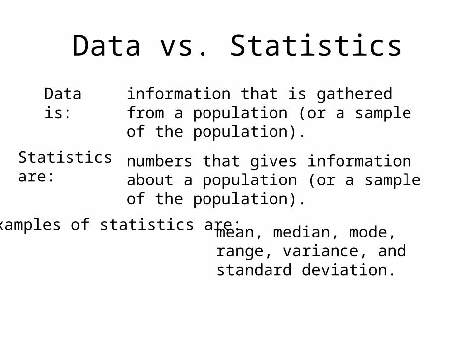
Data vs. Statistics

Data is:

Statistics are:

mean, median, mode, range, variance, and standard deviation.

numbers that gives information about a population (or a sample of the population).

Examples of statistics are:

information that is gathered from a population (or a sample of the population).

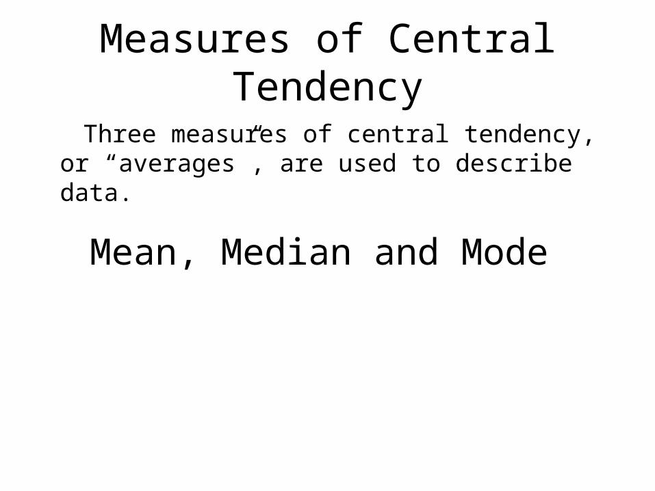
Measures of Central Tendency

Three measures of central tendency, or “averages”, are used to describe data.

Mean, Median and Mode

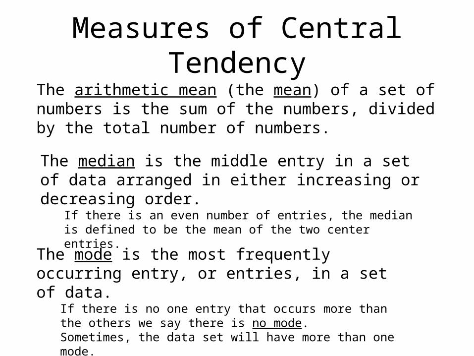
Measures of Central TendencyThe arithmetic mean (the mean) of a set of numbers is the sum of the numbers, divided by the total number of numbers.

The median is the middle entry in a set of data arranged in either increasing or decreasing order.

If there is an even number of entries, the median is defined to be the mean of the two center entries.

The mode is the most frequently occurring entry, or entries, in a set of data.

If there is no one entry that occurs more than the others we say there is no mode. Sometimes, the data set will have more than one mode.

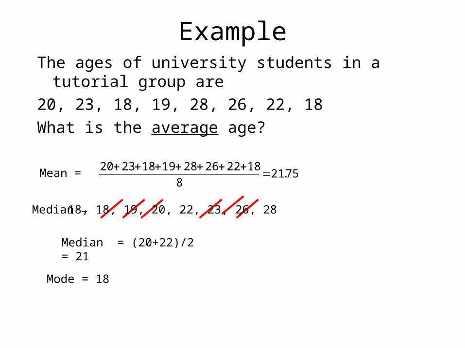
ExampleThe ages of university students in a tutorial group are

20, 23, 18, 19, 28, 26, 22, 18

What is the average age?

Mean =

Median →

75.218

1822262819182320

Median = (20+22)/2 = 21

Mode = 18

18, 18, 19, 20, 22, 23, 26, 28

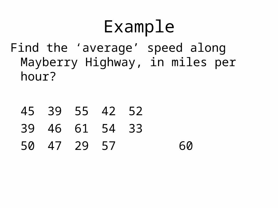
ExampleFind the ‘average’ speed along Mayberry

Highway, in miles per hour?

45 39 55 42 52

39 46 61 54 33

50 47 29 57 60

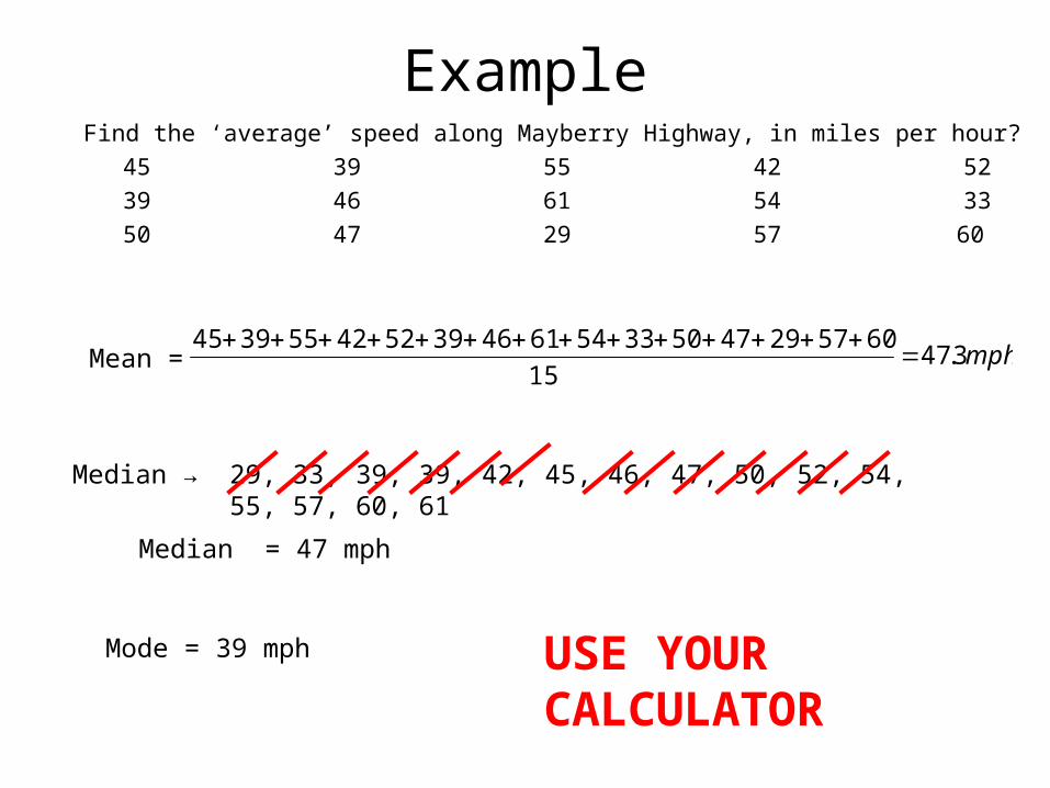
ExampleFind the ‘average’ speed along Mayberry Highway, in miles per hour?

45 39 55 42 52

39 46 61 54 33

50 47 29 57 60

Mean =

Median →

mph3.4715

605729475033546146395242553945

29, 33, 39, 39, 42, 45, 46, 47, 50, 52, 54, 55, 57, 60, 61

Median = 47 mph

Mode = 39 mph USE YOUR CALCULATOR

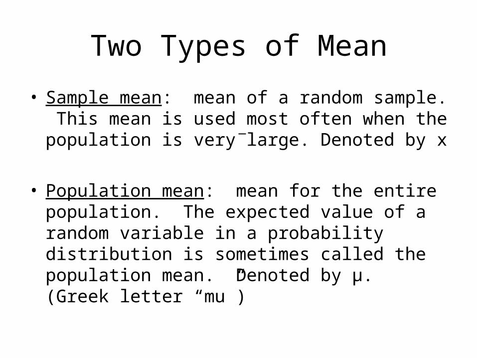
Two Types of Mean

• Sample mean: mean of a random sample. This mean is used most often when the population is very large. Denoted by x

• Population mean: mean for the entire population. The expected value of a random variable in a probability distribution is sometimes called the population mean. Denoted by µ. (Greek letter “mu”)

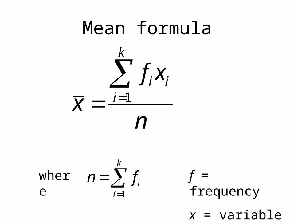
Mean formula

n

xfx

k

iii

1

where

k

iifn

1

f = frequency

x = variable

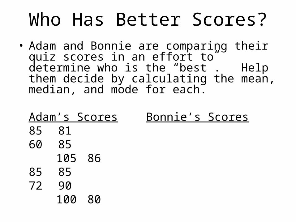
Who Has Better Scores?• Adam and Bonnie are comparing their quiz

scores in an effort to determine who is the “best”. Help them decide by calculating the mean, median, and mode for each.

Adam’s Scores Bonnie’s Scores85 8160 85

105 8685 8572 90

100 80

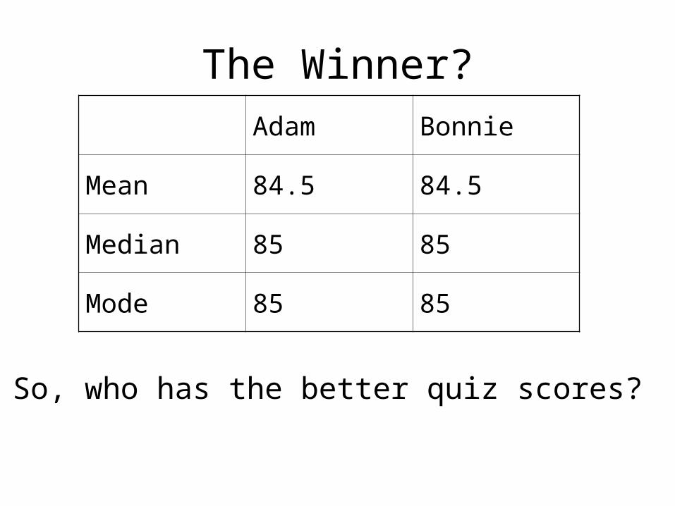
The Winner?Adam Bonnie

Mean 84.5 84.5

Median 85 85

Mode 85 85

So, who has the better quiz scores?

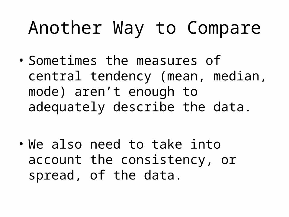
Another Way to Compare

• Sometimes the measures of central tendency (mean, median, mode) aren’t enough to adequately describe the data.

• We also need to take into account the consistency, or spread, of the data.

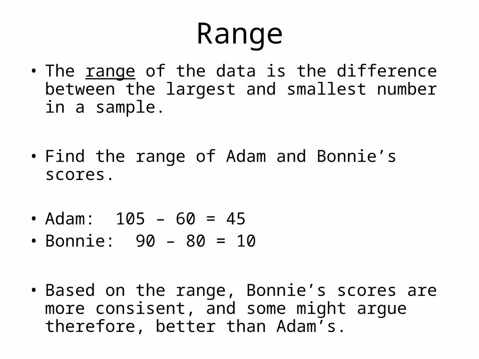
Range• The range of the data is the difference between

the largest and smallest number in a sample.

• Find the range of Adam and Bonnie’s scores.

• Adam: 105 – 60 = 45• Bonnie: 90 – 80 = 10

• Based on the range, Bonnie’s scores are more consisent, and some might argue therefore, better than Adam’s.

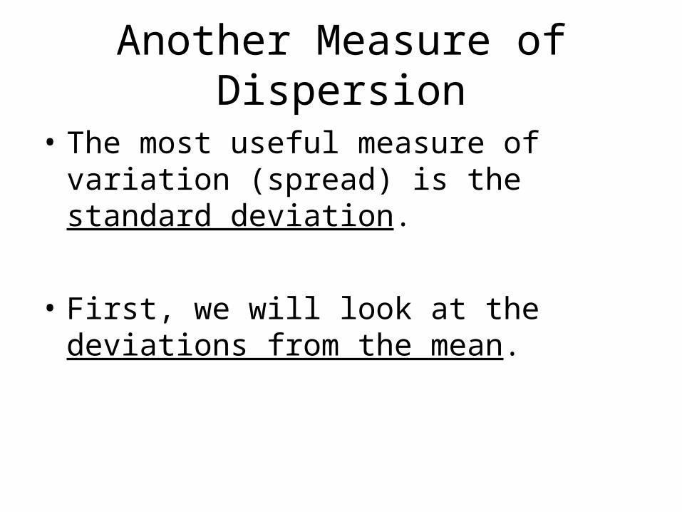
Another Measure of Dispersion

• The most useful measure of variation (spread) is the standard deviation.

• First, we will look at the deviations from the mean.

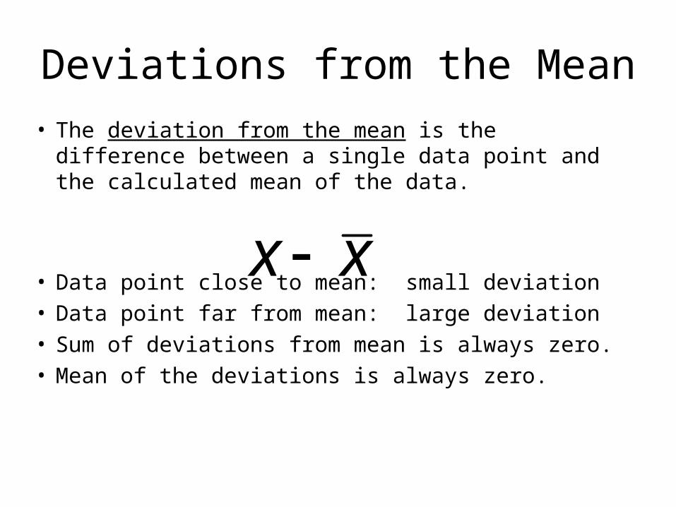
Deviations from the Mean

• The deviation from the mean is the difference between a single data point and the calculated mean of the data.

• Data point close to mean: small deviation• Data point far from mean: large deviation• Sum of deviations from mean is always zero.• Mean of the deviations is always zero.

xx

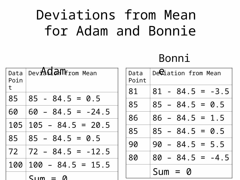
Deviations from Mean for Adam and Bonnie

Data Point

Deviation from Mean

85 85 - 84.5 = 0.5

60 60 – 84.5 = -24.5

105 105 – 84.5 = 20.5

85 85 – 84.5 = 0.5

72 72 – 84.5 = -12.5

100 100 – 84.5 = 15.5

Sum = 0

AdamData Point

Deviation from Mean

81 81 - 84.5 = -3.5

85 85 – 84.5 = 0.5

86 86 – 84.5 = 1.5

85 85 – 84.5 = 0.5

90 90 – 84.5 = 5.5

80 80 – 84.5 = -4.5

Sum = 0

Bonnie

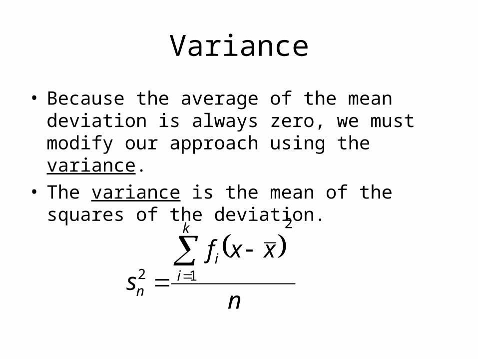
Variance

• Because the average of the mean deviation is always zero, we must modify our approach using the variance.

• The variance is the mean of the squares of the deviation.

n

xxfs

k

ii

n

2

12

Variance for Adam and Bonnie’s Scores

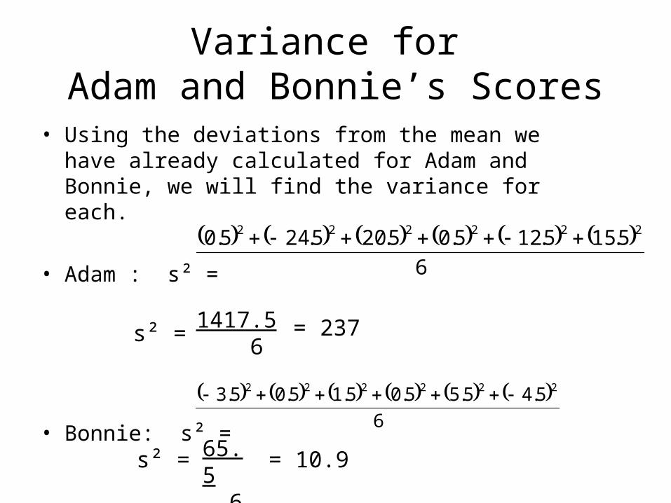
• Using the deviations from the mean we have already calculated for Adam and Bonnie, we will find the variance for each.

• Adam : s² =

• Bonnie: s² =

6

5.155.125.05.205.245.0 222222

s² = 1417.5 6

= 237

s² = 65.5 6

= 10.9

6

5.45.55.05.15.05.3 222222

Standard Deviation

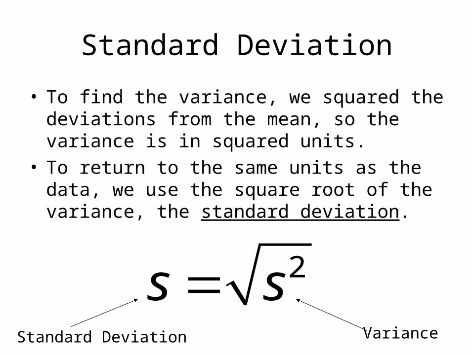
• To find the variance, we squared the deviations from the mean, so the variance is in squared units.

• To return to the same units as the data, we use the square root of the variance, the standard deviation.

2s sStandard Deviation Variance

Adam and Bonnie’s Standard Deviation

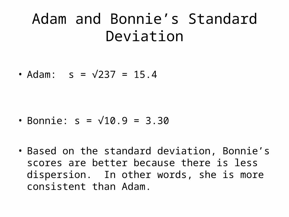
• Adam: s = √237 = 15.4

• Bonnie: s = √10.9 = 3.30

• Based on the standard deviation, Bonnie’s scores are better because there is less dispersion. In other words, she is more consistent than Adam.

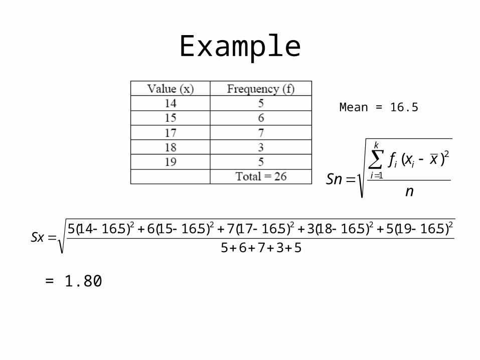
Example

53765

)5.1619(5)5.1618(3)5.1617(7)5.1615(6)5.1614(5 22222

Sx

= 1.80

n

xxfSn

k

iii

1

2)(

Mean = 16.5

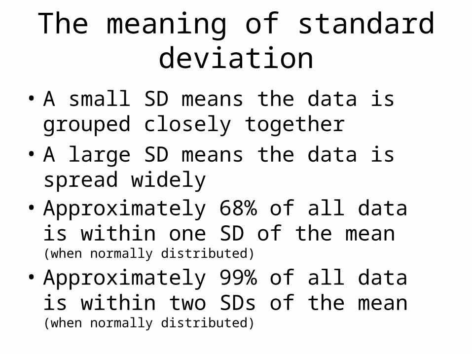
The meaning of standard deviation

• A small SD means the data is grouped closely together

• A large SD means the data is spread widely

• Approximately 68% of all data is within one SD of the mean (when normally distributed)

• Approximately 99% of all data is within two SDs of the mean (when normally distributed)

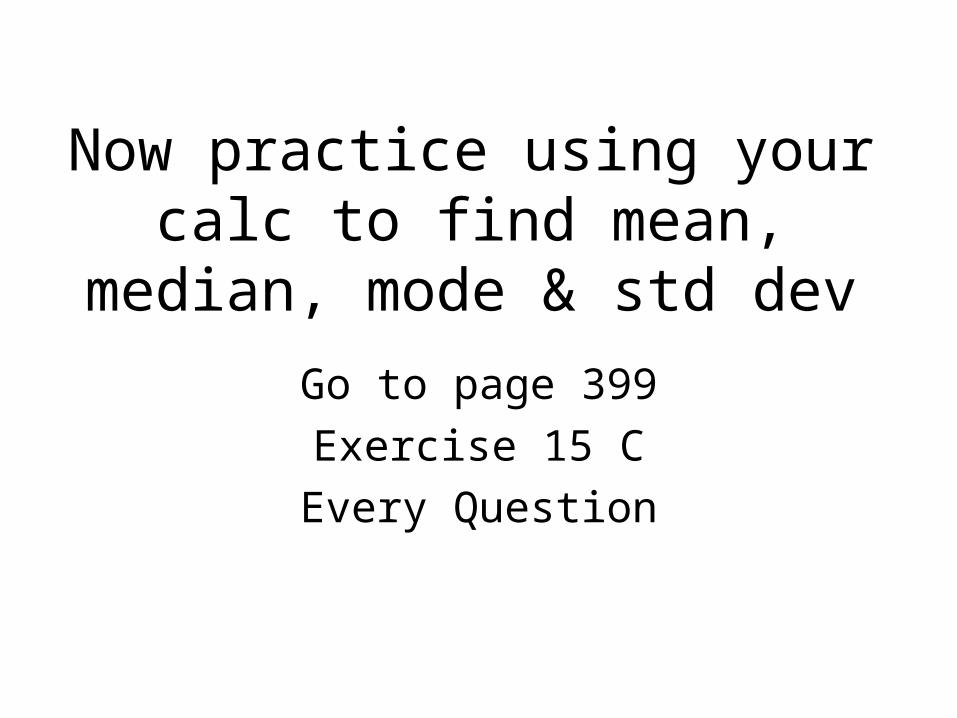
Now practice using your calc to find mean, median, mode &

std dev

Go to page 399

Exercise 15 C

Every Question