STATISTICS 7Basic Statistics

Professor Jessica Uttshttp://www.ics.uci.edu/~jutts/7

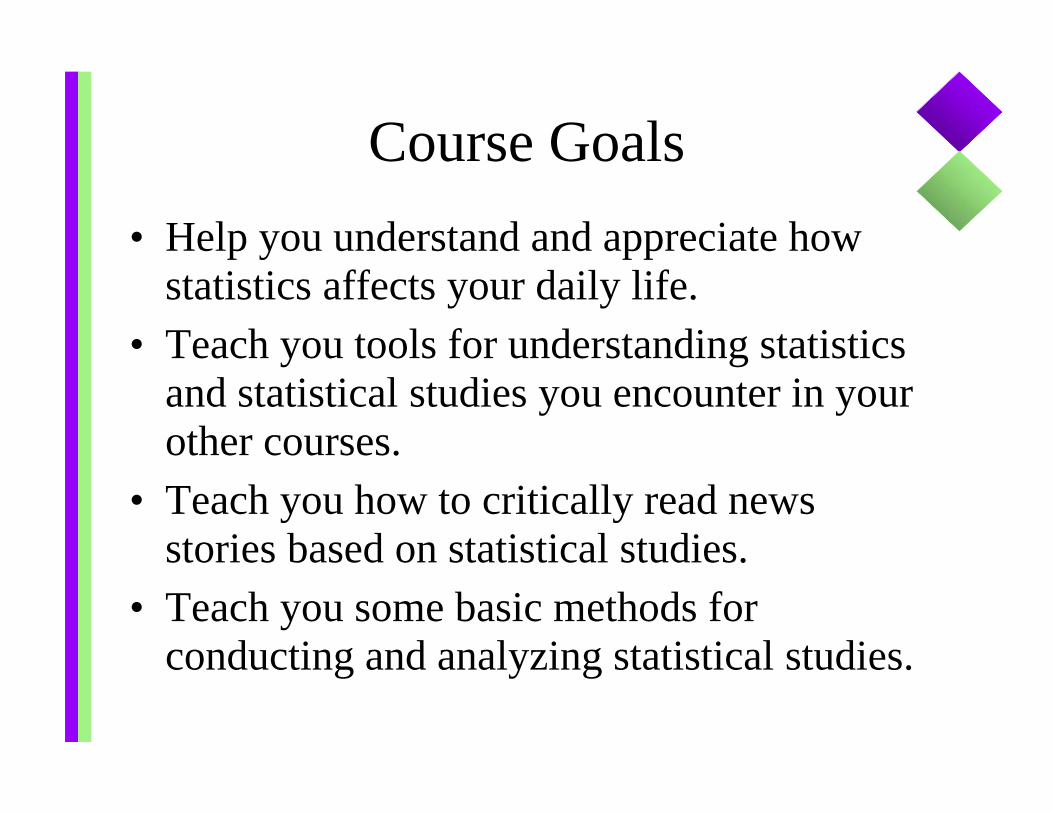
Course Goals• Help you understand and appreciate how

statistics affects your daily life.• Teach you tools for understanding statistics

and statistical studies you encounter in your other courses.

• Teach you how to critically read news stories based on statistical studies.

• Teach you some basic methods for conducting and analyzing statistical studies.

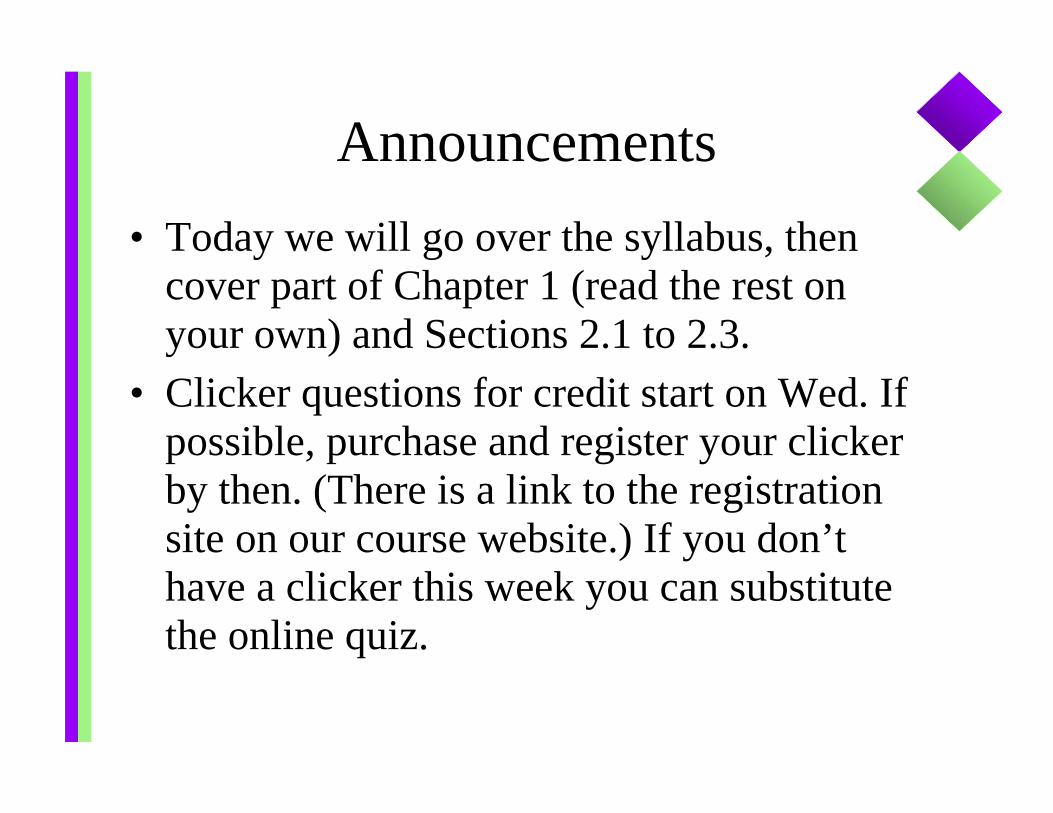
Announcements• Today we will go over the syllabus, then

cover part of Chapter 1 (read the rest on your own) and Sections 2.1 to 2.3.

• Clicker questions for credit start on Wed. If possible, purchase and register your clicker by then. (There is a link to the registration site on our course website.) If you don’t have a clicker this week you can substitute the online quiz.

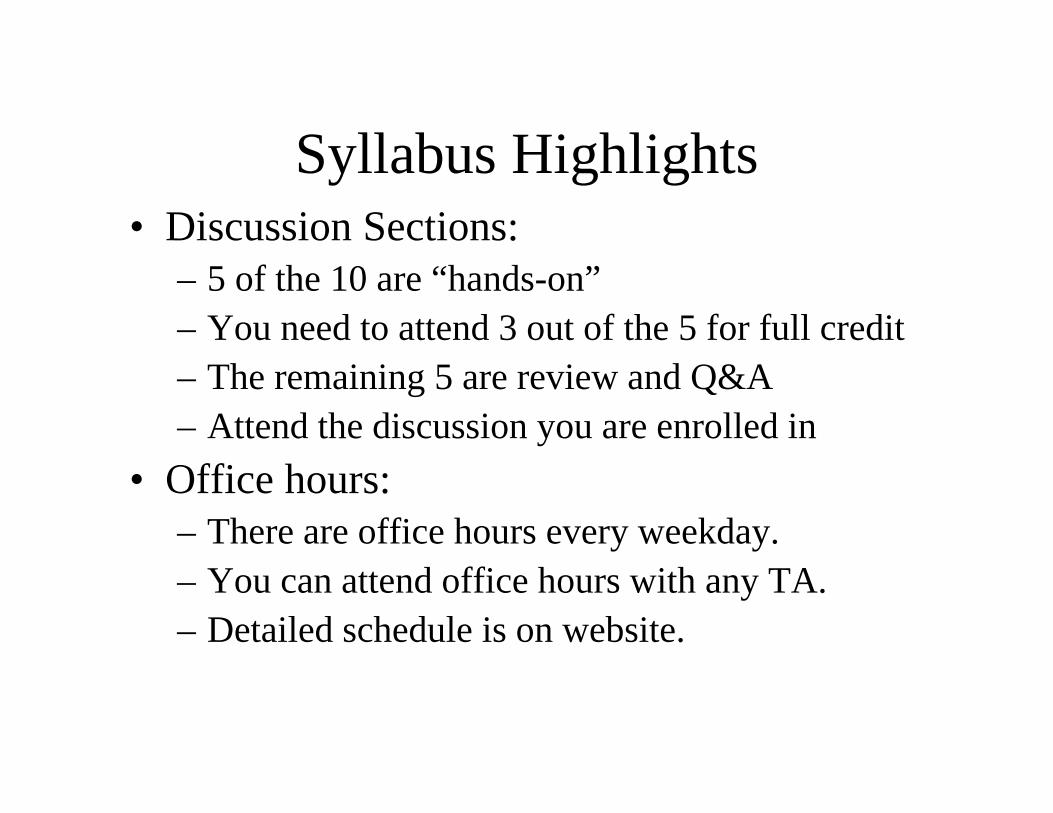
Syllabus Highlights• Discussion Sections:

– 5 of the 10 are “hands-on”– You need to attend 3 out of the 5 for full credit– The remaining 5 are review and Q&A– Attend the discussion you are enrolled in

• Office hours: – There are office hours every weekday.– You can attend office hours with any TA.– Detailed schedule is on website.

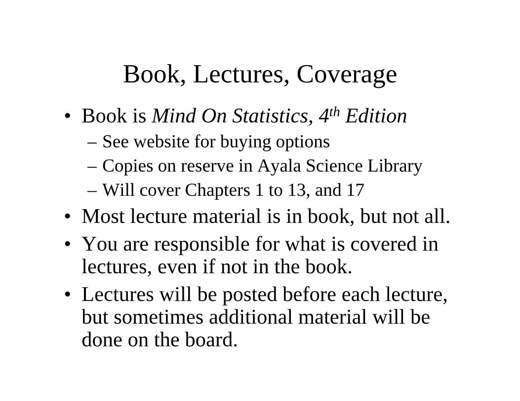
Book, Lectures, Coverage• Book is Mind On Statistics, 4th Edition

– See website for buying options– Copies on reserve in Ayala Science Library– Will cover Chapters 1 to 13, and 17

• Most lecture material is in book, but not all.• You are responsible for what is covered in

lectures, even if not in the book.• Lectures will be posted before each lecture,

but sometimes additional material will be done on the board.

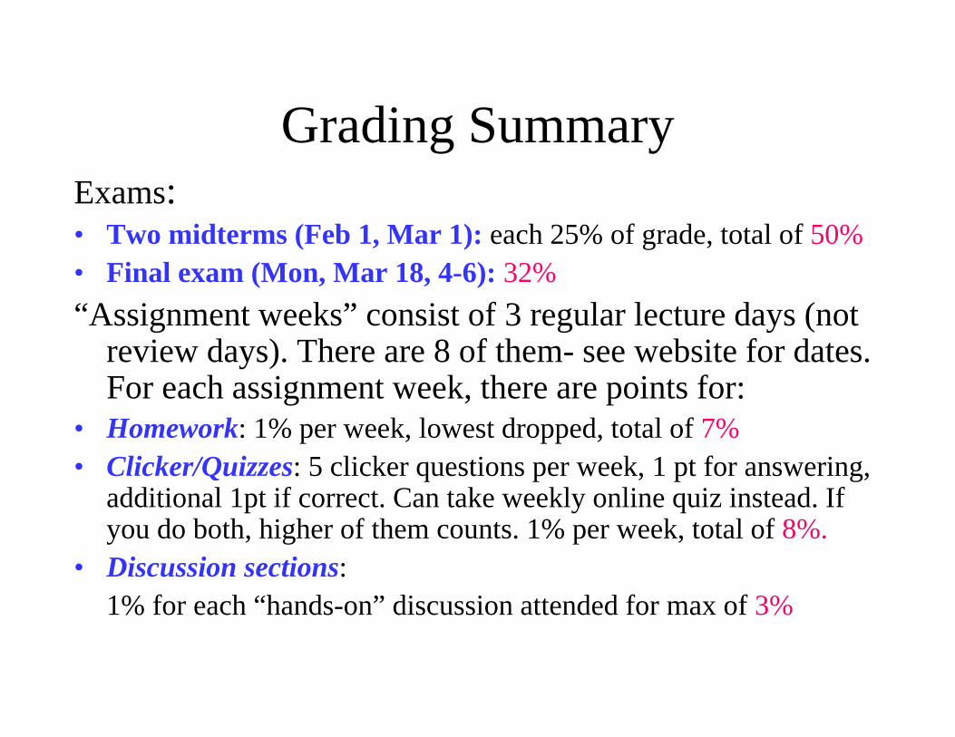
Grading SummaryExams:• Two midterms (Feb 1, Mar 1): each 25% of grade, total of 50%• Final exam (Mon, Mar 18, 4-6): 32%“Assignment weeks” consist of 3 regular lecture days (not

review days). There are 8 of them- see website for dates. For each assignment week, there are points for:

• Homework: 1% per week, lowest dropped, total of 7%• Clicker/Quizzes: 5 clicker questions per week, 1 pt for answering,

additional 1pt if correct. Can take weekly online quiz instead. If you do both, higher of them counts. 1% per week, total of 8%.

• Discussion sections: 1% for each “hands-on” discussion attended for max of 3%

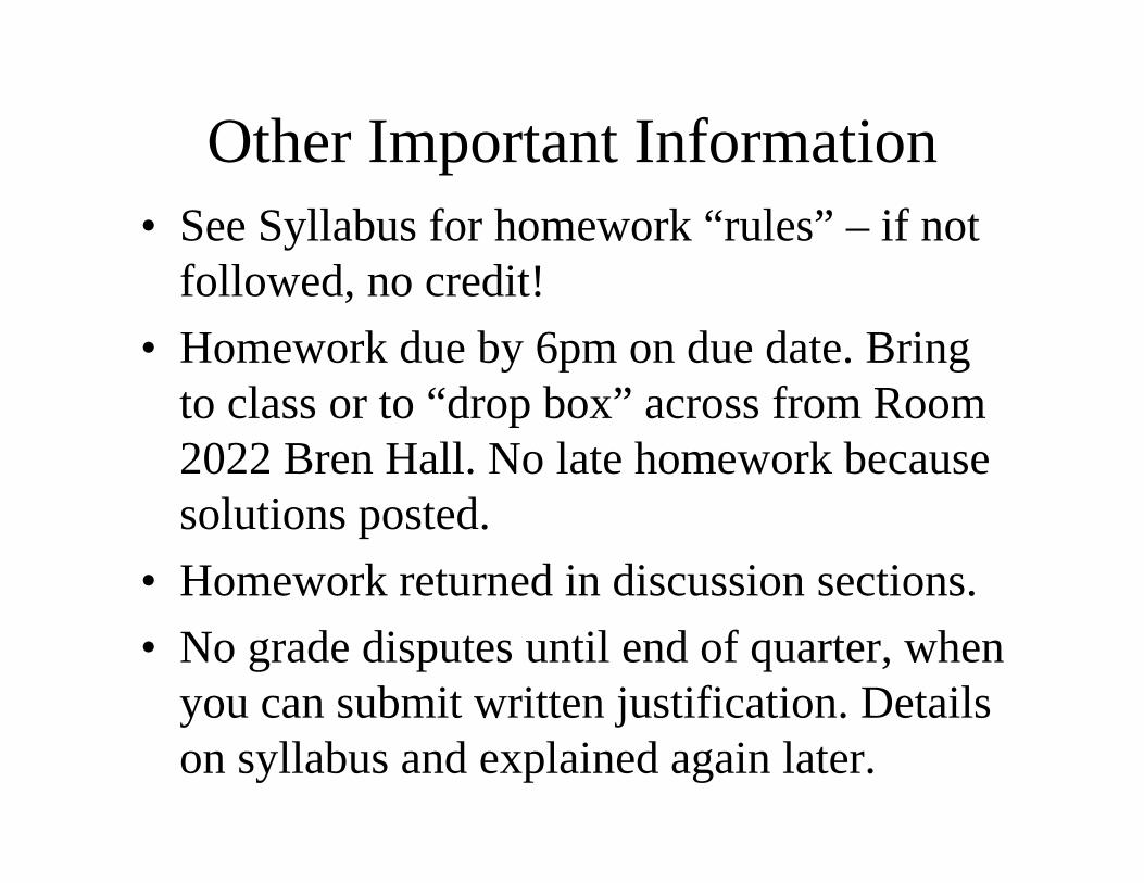
Other Important Information• See Syllabus for homework “rules” – if not

followed, no credit!• Homework due by 6pm on due date. Bring

to class or to “drop box” across from Room 2022 Bren Hall. No late homework because solutions posted.

• Homework returned in discussion sections.• No grade disputes until end of quarter, when

you can submit written justification. Details on syllabus and explained again later.

Classroom Etiquette

• I try to start and end on time. Please respect the 50 minutes of class time.

• Silence electronics, but okay to have them on.

• If you are bored feel free to do something else, but do not disturb others around you.

• If you know you need to leave early, try to sit near the door.

Statistics Success Stories

and Cautionary

Tales

Chapter 1

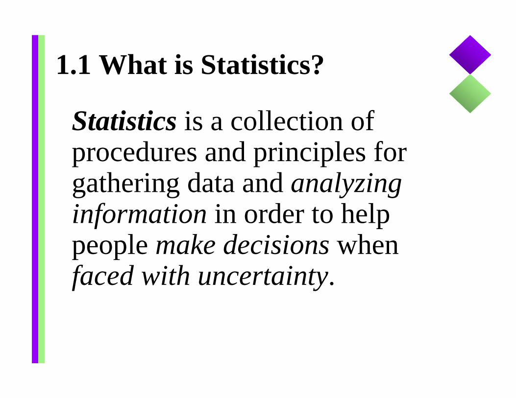
1.1 What is Statistics?

Statistics is a collection of procedures and principles for gathering data and analyzing information in order to help people make decisions when faced with uncertainty.

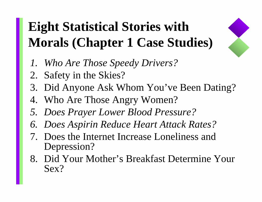
Eight Statistical Stories with Morals (Chapter 1 Case Studies)1. Who Are Those Speedy Drivers?2. Safety in the Skies?3. Did Anyone Ask Whom You’ve Been Dating?4. Who Are Those Angry Women?5. Does Prayer Lower Blood Pressure?6. Does Aspirin Reduce Heart Attack Rates?7. Does the Internet Increase Loneliness and

Depression?8. Did Your Mother’s Breakfast Determine Your

Sex?

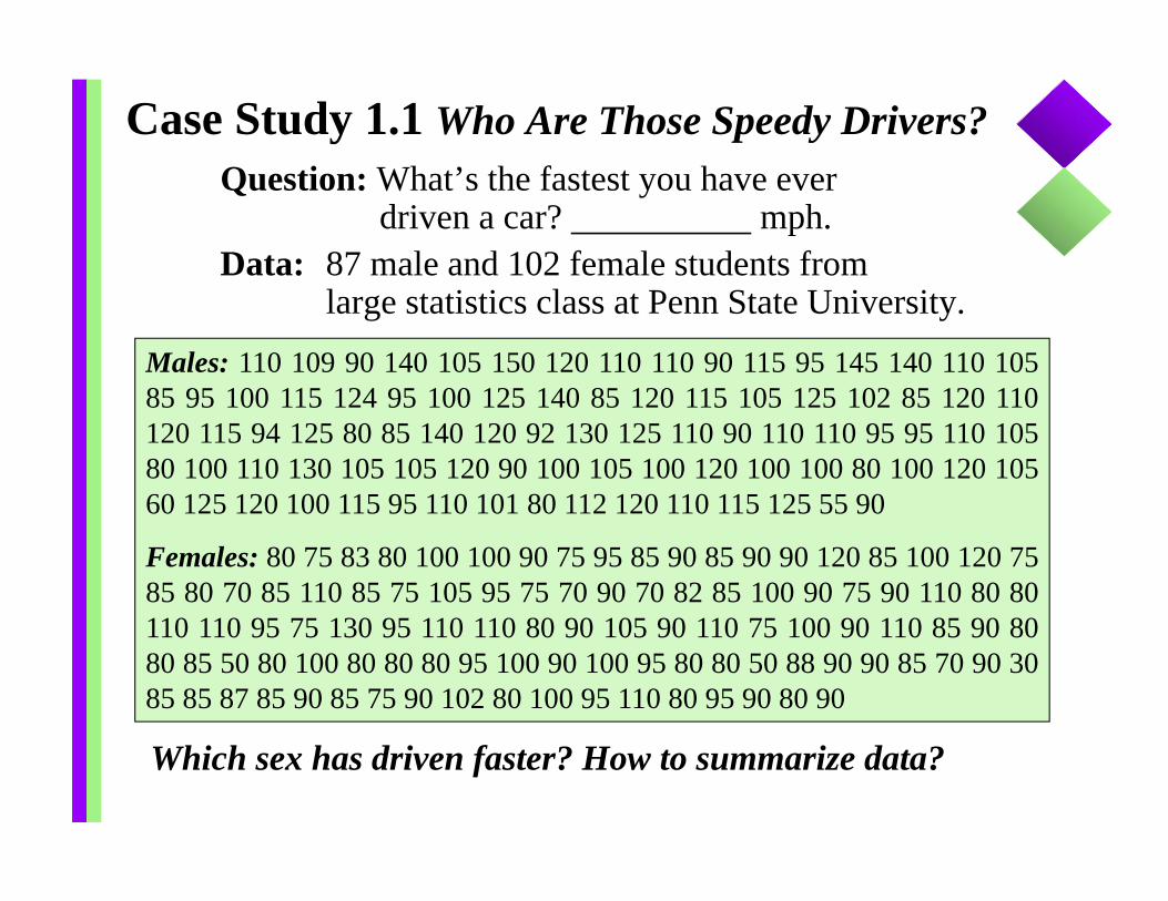
Case Study 1.1 Who Are Those Speedy Drivers?Question: What’s the fastest you have ever

driven a car? mph.Data: 87 male and 102 female students from

large statistics class at Penn State University.

Males: 110 109 90 140 105 150 120 110 110 90 115 95 145 140 110 10585 95 100 115 124 95 100 125 140 85 120 115 105 125 102 85 120 110120 115 94 125 80 85 140 120 92 130 125 110 90 110 110 95 95 110 10580 100 110 130 105 105 120 90 100 105 100 120 100 100 80 100 120 10560 125 120 100 115 95 110 101 80 112 120 110 115 125 55 90

Females: 80 75 83 80 100 100 90 75 95 85 90 85 90 90 120 85 100 120 7585 80 70 85 110 85 75 105 95 75 70 90 70 82 85 100 90 75 90 110 80 80110 110 95 75 130 95 110 110 80 90 105 90 110 75 100 90 110 85 90 8080 85 50 80 100 80 80 80 95 100 90 100 95 80 80 50 88 90 90 85 70 90 3085 85 87 85 90 85 75 90 102 80 100 95 110 80 95 90 80 90

Which sex has driven faster? How to summarize data?

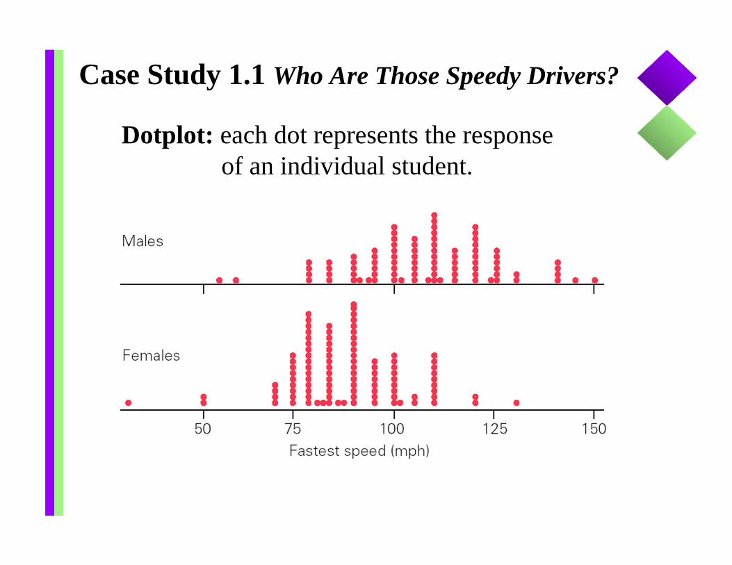
Case Study 1.1 Who Are Those Speedy Drivers?

Dotplot: each dot represents the response of an individual student.

Case Study 1.1 Who Are Those Speedy Drivers?

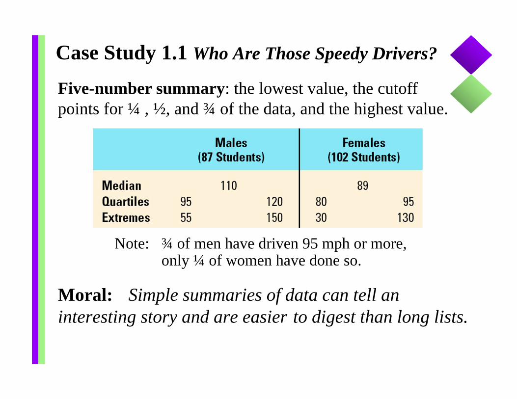
Five-number summary: the lowest value, the cutoff points for ¼ , ½, and ¾ of the data, and the highest value.

Note: ¾ of men have driven 95 mph or more, only ¼ of women have done so.

Moral: Simple summaries of data can tell an interesting story and are easier to digest than long lists.

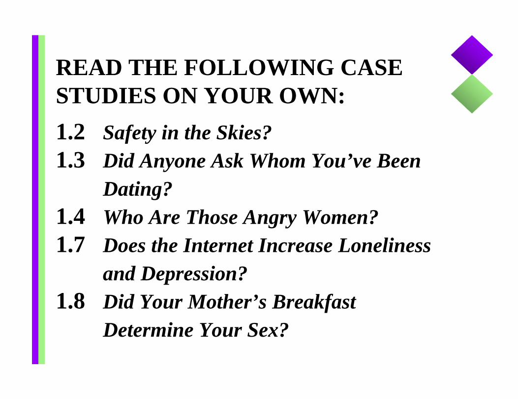
READ THE FOLLOWING CASE STUDIES ON YOUR OWN:1.2 Safety in the Skies?1.3 Did Anyone Ask Whom You’ve Been

Dating?1.4 Who Are Those Angry Women?1.7 Does the Internet Increase Loneliness

and Depression?1.8 Did Your Mother’s Breakfast

Determine Your Sex?

Case Study 1.5 Does Prayer Lower Blood Pressure?

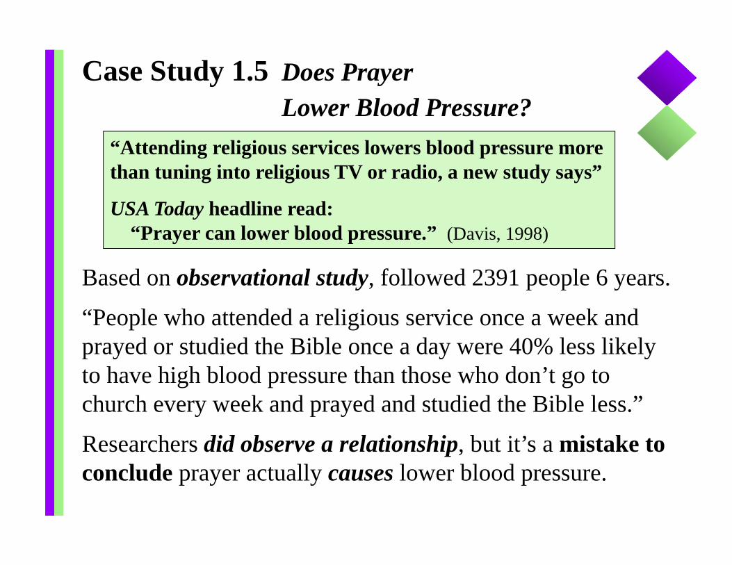
“Attending religious services lowers blood pressure more than tuning into religious TV or radio, a new study says”

USA Today headline read: “Prayer can lower blood pressure.” (Davis, 1998)

Based on observational study, followed 2391 people 6 years.

“People who attended a religious service once a week and prayed or studied the Bible once a day were 40% less likely to have high blood pressure than those who don’t go to church every week and prayed and studied the Bible less.”

Researchers did observe a relationship, but it’s a mistake to conclude prayer actually causes lower blood pressure.

Case Study 1.5 Does Prayer Lower Blood Pressure?

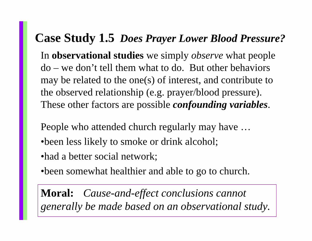
Moral: Cause-and-effect conclusions cannot generally be made based on an observational study.

In observational studies we simply observe what people do – we don’t tell them what to do. But other behaviors may be related to the one(s) of interest, and contribute to the observed relationship (e.g. prayer/blood pressure). These other factors are possible confounding variables.

People who attended church regularly may have …•been less likely to smoke or drink alcohol;•had a better social network;•been somewhat healthier and able to go to church.

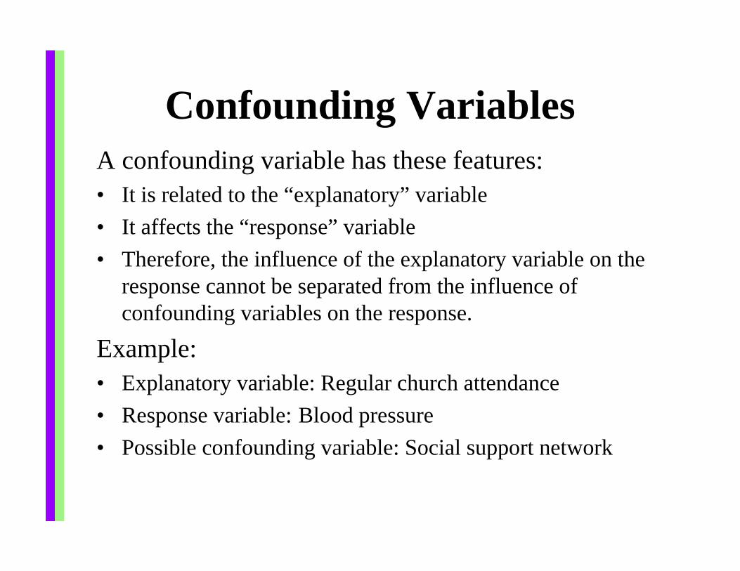
Confounding VariablesA confounding variable has these features:• It is related to the “explanatory” variable• It affects the “response” variable• Therefore, the influence of the explanatory variable on the

response cannot be separated from the influence of confounding variables on the response.

Example:• Explanatory variable: Regular church attendance• Response variable: Blood pressure• Possible confounding variable: Social support network

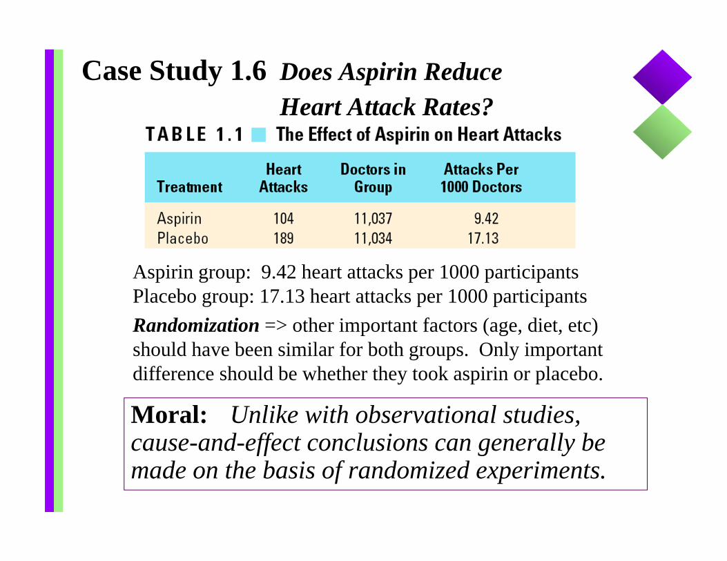
Case Study 1.6 Does Aspirin Reduce Heart Attack Rates?

Physician’s Health Study (1988)5-year randomized experiment …

• 22,071 male physicians of age 40 - 84;• randomly assigned to one

of two treatment groups;• Group 1 = aspirin every other day;

Group 2 = placebo;• Physicians blinded as to which group

they were in.

Case Study 1.6 Does Aspirin Reduce Heart Attack Rates?

Moral: Unlike with observational studies, cause-and-effect conclusions can generally be made on the basis of randomized experiments.

Aspirin group: 9.42 heart attacks per 1000 participantsPlacebo group: 17.13 heart attacks per 1000 participantsRandomization => other important factors (age, diet, etc) should have been similar for both groups. Only important difference should be whether they took aspirin or placebo.

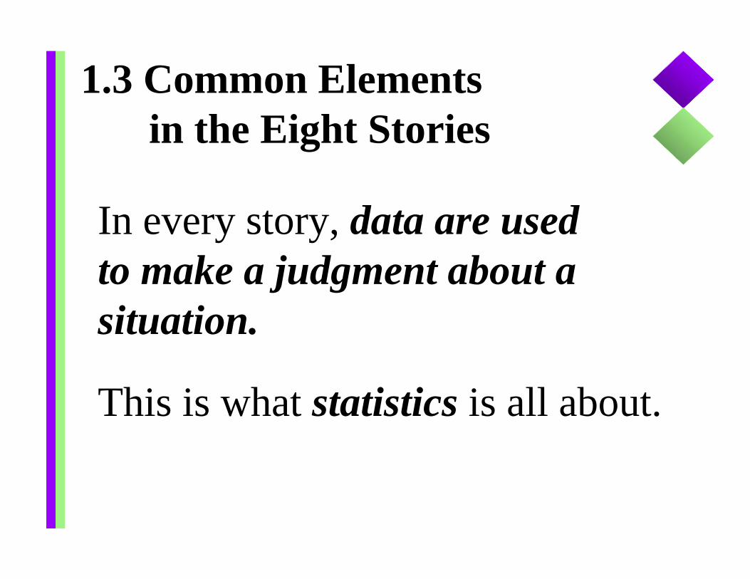
1.3 Common Elementsin the Eight Stories

In every story, data are used to make a judgment about a situation.

This is what statistics is all about.

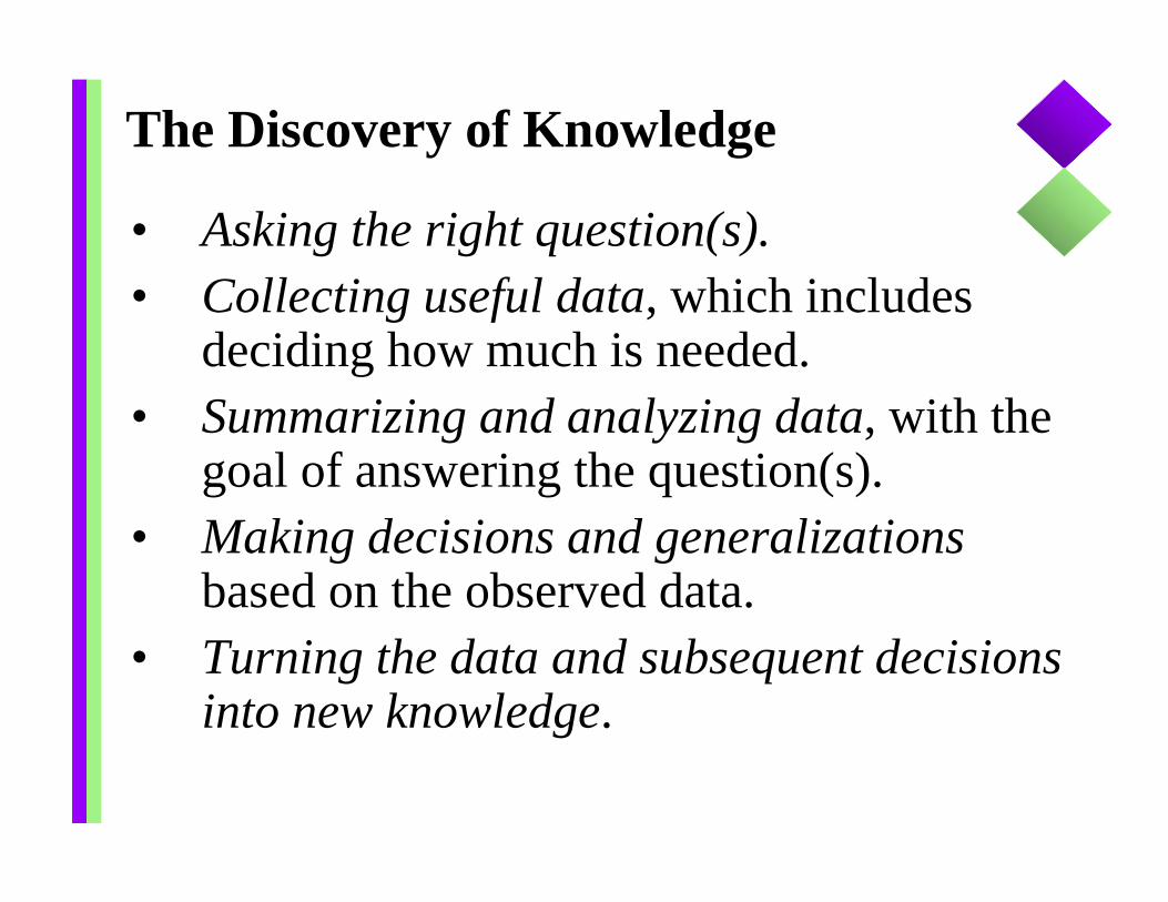
The Discovery of Knowledge

• Asking the right question(s).• Collecting useful data, which includes

deciding how much is needed.• Summarizing and analyzing data, with the

goal of answering the question(s).• Making decisions and generalizations

based on the observed data.• Turning the data and subsequent decisions

into new knowledge.

Turning Data Into

InformationChapter 2

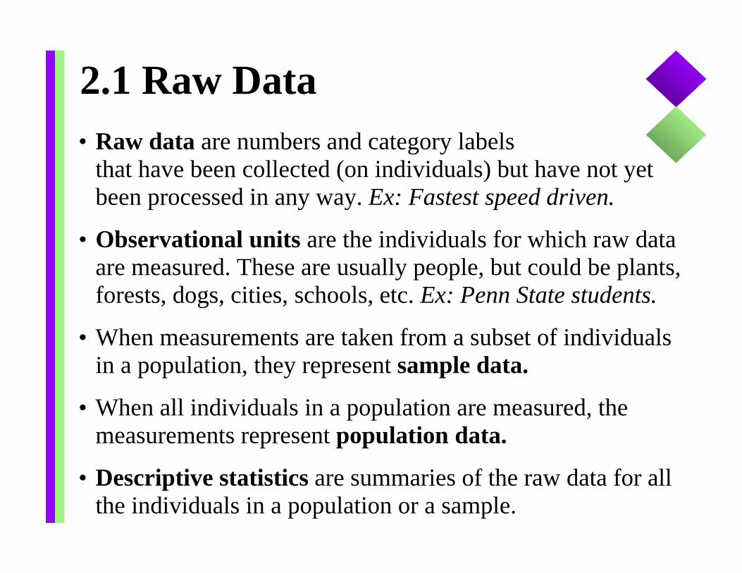
2.1 Raw Data• Raw data are numbers and category labels

that have been collected (on individuals) but have not yet been processed in any way. Ex: Fastest speed driven.

• Observational units are the individuals for which raw data are measured. These are usually people, but could be plants, forests, dogs, cities, schools, etc. Ex: Penn State students.

• When measurements are taken from a subset of individuals in a population, they represent sample data.

• When all individuals in a population are measured, the measurements represent population data.

• Descriptive statistics are summaries of the raw data for all the individuals in a population or a sample.

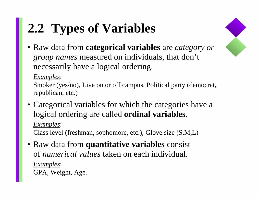
2.2 Types of Variables• Raw data from categorical variables are category or

group names measured on individuals, that don’t necessarily have a logical ordering. Examples: Smoker (yes/no), Live on or off campus, Political party (democrat, republican, etc.)

• Categorical variables for which the categories have a logical ordering are called ordinal variables.Examples: Class level (freshman, sophomore, etc.), Glove size (S,M,L)

• Raw data from quantitative variables consist of numerical values taken on each individual. Examples: GPA, Weight, Age.

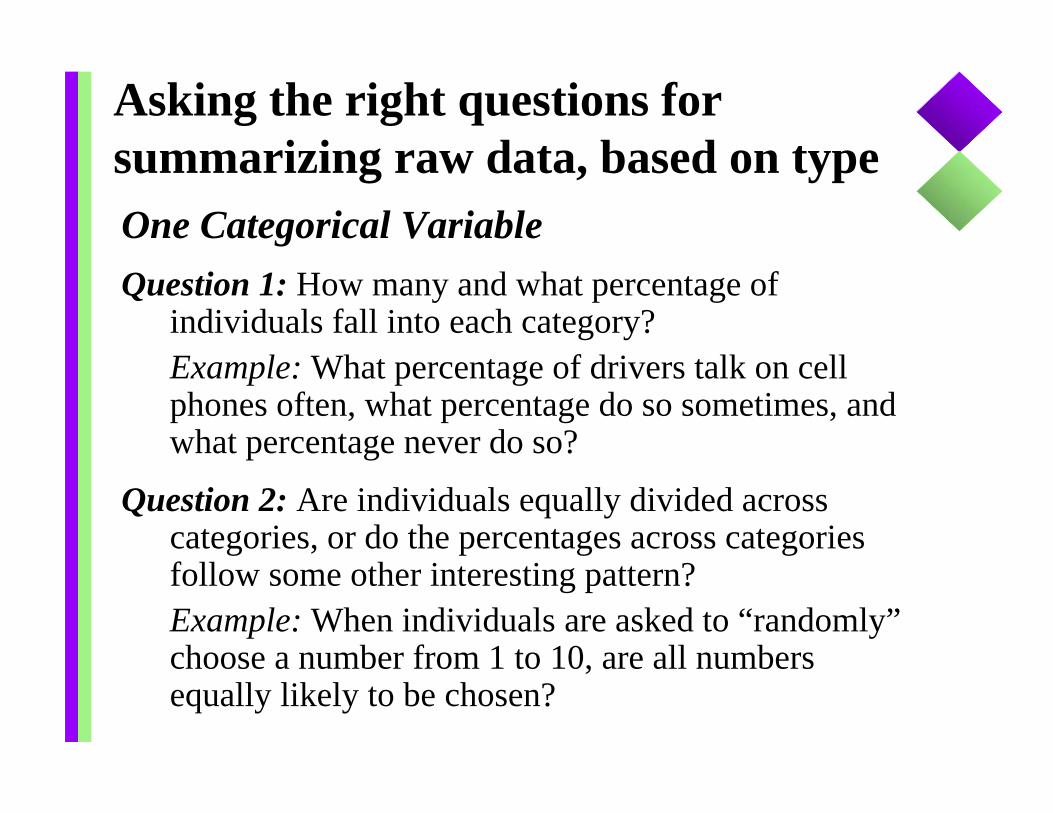
Asking the right questions for summarizing raw data, based on typeOne Categorical VariableQuestion 1: How many and what percentage of

individuals fall into each category?Example: What percentage of drivers talk on cell phones often, what percentage do so sometimes, and what percentage never do so?

Question 2: Are individuals equally divided across categories, or do the percentages across categories follow some other interesting pattern?Example: When individuals are asked to “randomly” choose a number from 1 to 10, are all numbers equally likely to be chosen?

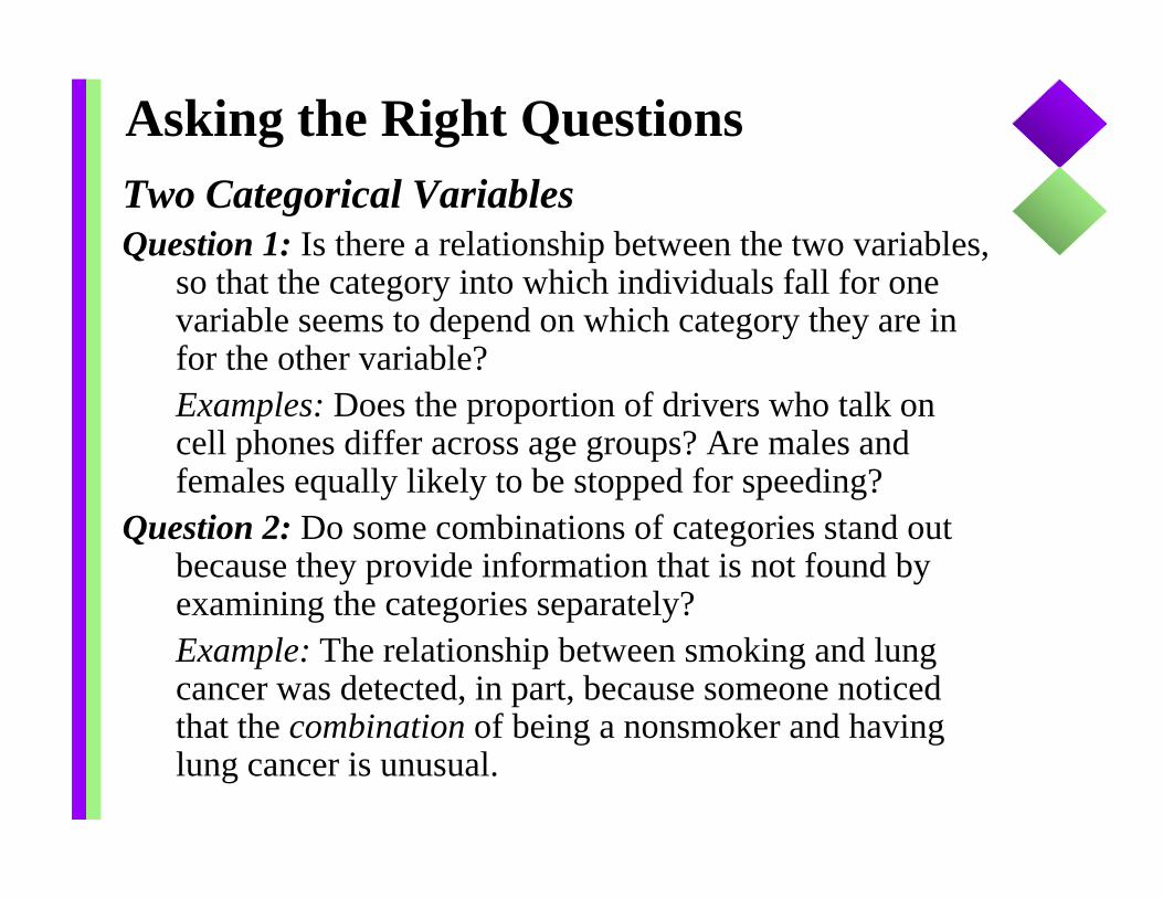
Asking the Right QuestionsTwo Categorical VariablesQuestion 1: Is there a relationship between the two variables,

so that the category into which individuals fall for one variable seems to depend on which category they are in for the other variable?Examples: Does the proportion of drivers who talk on cell phones differ across age groups? Are males and females equally likely to be stopped for speeding?

Question 2: Do some combinations of categories stand out because they provide information that is not found by examining the categories separately?Example: The relationship between smoking and lung cancer was detected, in part, because someone noticed that the combination of being a nonsmoker and having lung cancer is unusual.

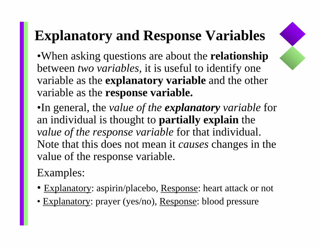
Explanatory and Response Variables•When asking questions are about the relationshipbetween two variables, it is useful to identify one variable as the explanatory variable and the other variable as the response variable. •In general, the value of the explanatory variable for an individual is thought to partially explain the value of the response variable for that individual. Note that this does not mean it causes changes in the value of the response variable.Examples:• Explanatory: aspirin/placebo, Response: heart attack or not• Explanatory: prayer (yes/no), Response: blood pressure

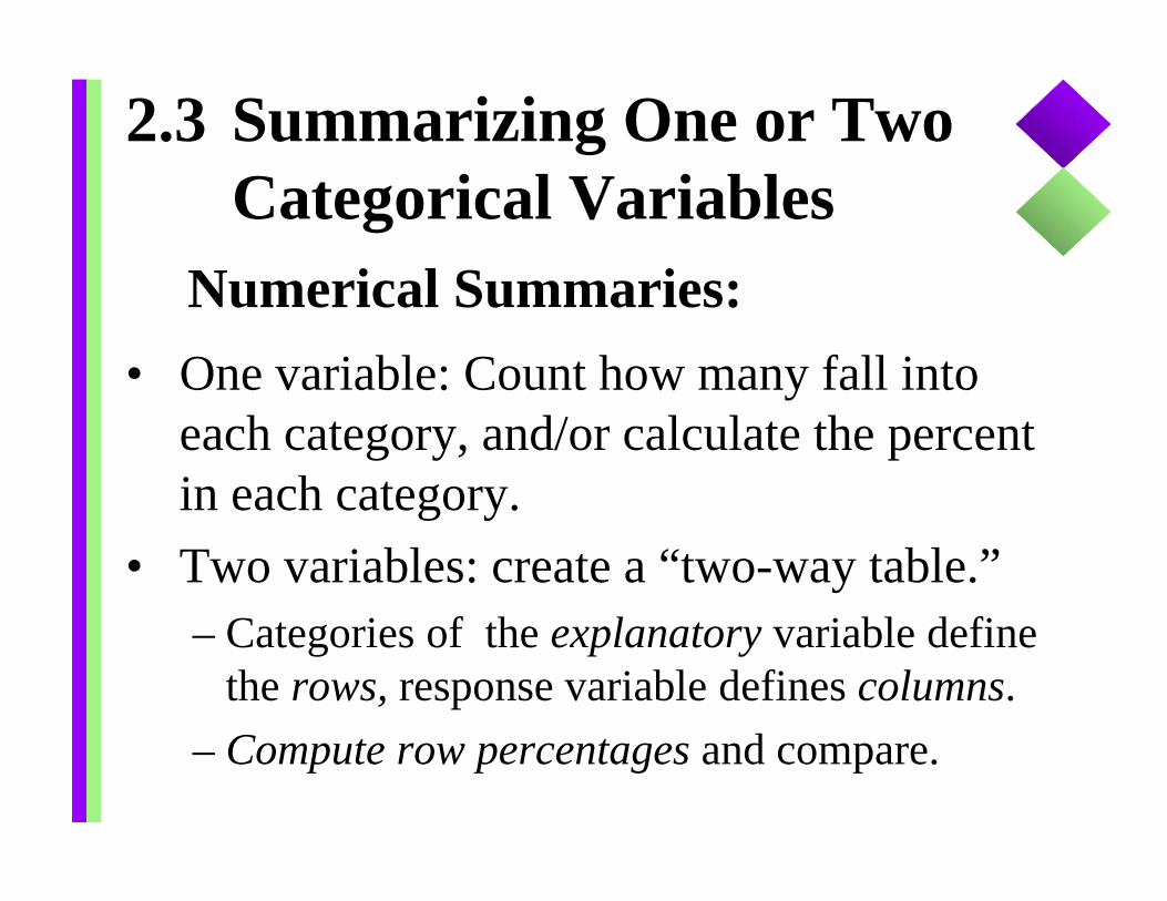
2.3 Summarizing One or TwoCategorical Variables

• One variable: Count how many fall into each category, and/or calculate the percent in each category.

• Two variables: create a “two-way table.” – Categories of the explanatory variable define

the rows, response variable defines columns.– Compute row percentages and compare.

Numerical Summaries:

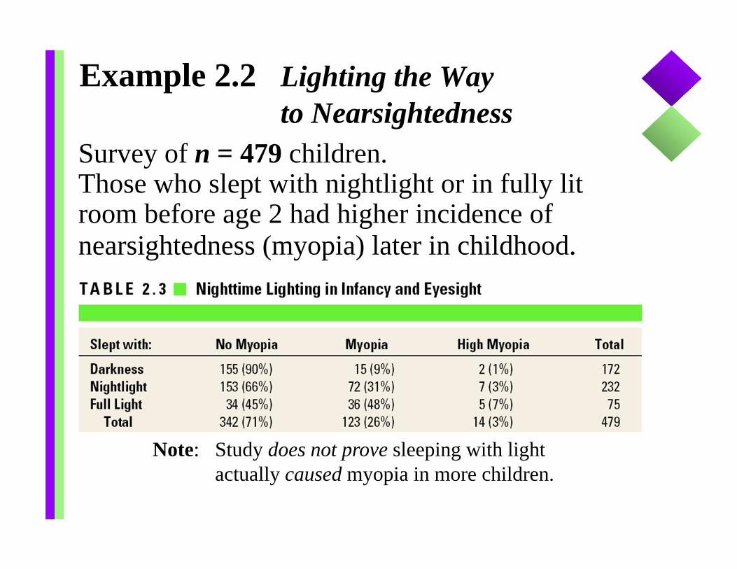
Example 2.2 Lighting the Way to Nearsightedness

Survey of n = 479 children. Those who slept with nightlight or in fully lit room before age 2 had higher incidence of nearsightedness (myopia) later in childhood.

Note: Study does not prove sleeping with light actually caused myopia in more children.

• Pie Charts: useful for summarizing a single categorical variable if not too many categories.

• Bar Graphs: useful for summarizing one or two categorical variables and particularly useful for making comparisons when there are two categorical variables.

Graphical (Visual) Summaries for Categorical Variables

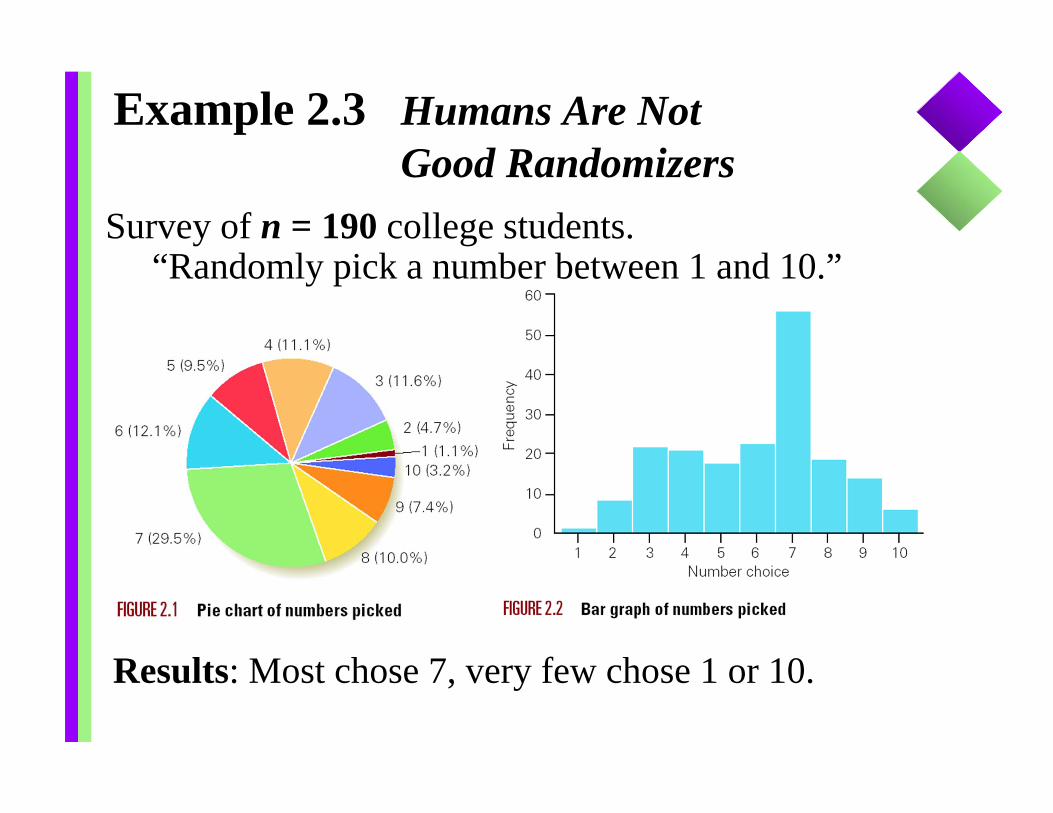
Example 2.3 Humans Are Not Good Randomizers

Survey of n = 190 college students. “Randomly pick a number between 1 and 10.”

Results: Most chose 7, very few chose 1 or 10.

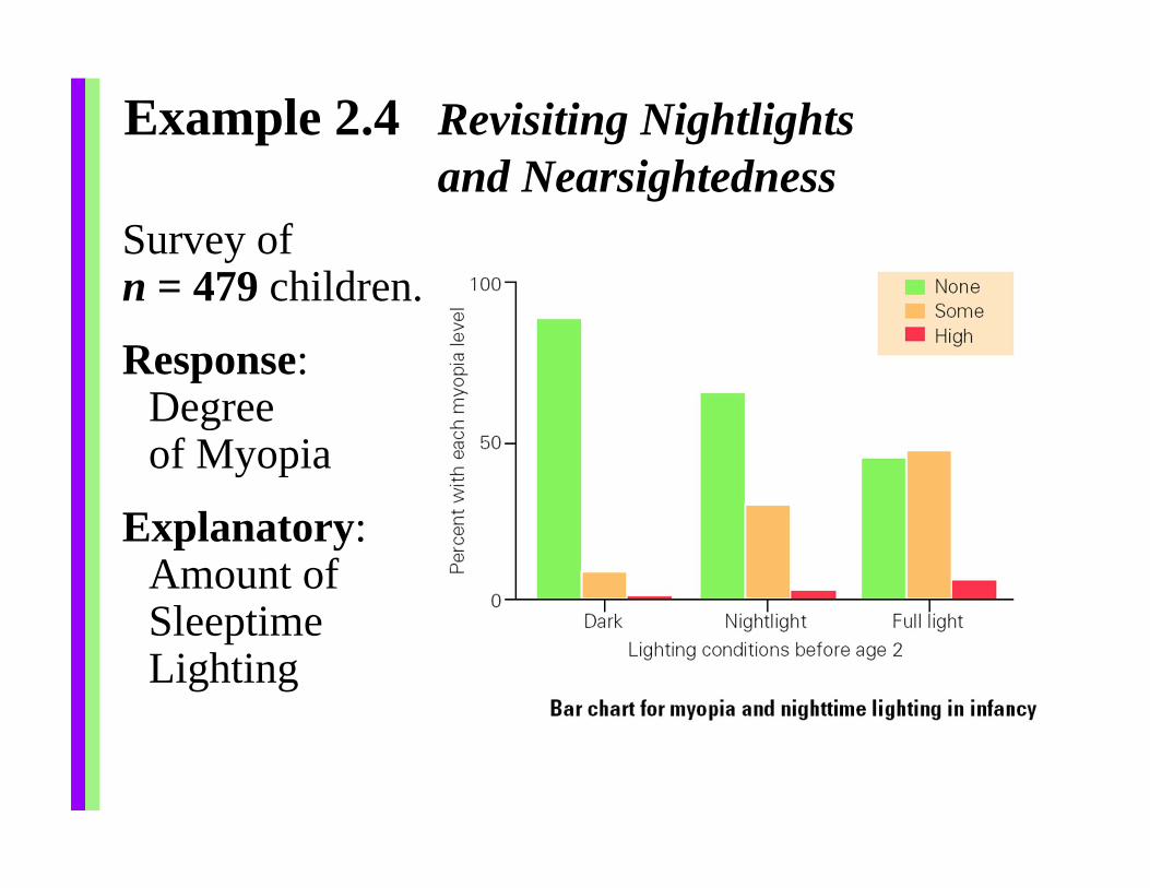
Example 2.4 Revisiting Nightlights and Nearsightedness

Survey of n = 479 children.

Response: Degree of Myopia

Explanatory:Amount of Sleeptime Lighting

• Recognize an observational study (no cause/effect) vs a randomized experiment:Exercise 1.25: Vegetarians had lower heart disease and cancer death rates than non-vegetarians.Exercise 1.28: Volunteers randomly assigned to nicotine patch or placebo, 46% vs 20% quit.

• Explanatory variable/ response variableFor the two examples above?

• Categorical data/ quantitative data For the two examples above?

Summary of Key Points

Summarizing one categorical variable:• Pie Charts• Bar GraphsSummarizing two categorical variables:• Two-way table (explanatory variable as

rows)• Row percents (or column percents), use for

comparisons• Bar graphs (explanatory variable categories

as separate sets of bars)

• Read Chapter 1• Read Chapter 2, Sections 2.1 to 2.3 (mostly

covered in class)

Homework, due Mon, Jan 14: 1.14 (pg. 11), 1.16 (pg.11)2.20 (pg. 56), 2.28 (pg. 57)

Homework; Sections to Read