STATISTICS AND DATA INVESTIGATION AND INTERPRETATION … · where each observation falls into one of a number ... learning about data investigation and interpretation. ... be considered

4YEAR

DATA INVESTIGATION AND INTERPRETATIONThe Improving Mathematics Education in Schools (TIMES) Project

A guide for teachers - Year 4 June 2011

STATISTICS AND PROBABILITY Module 2

Data Investigation and Interpretation

(Statistics and Probability : Module 2)

For teachers of Primary and Secondary Mathematics

510

Cover design, Layout design and Typesetting by Claire Ho

The Improving Mathematics Education in Schools (TIMES)

Project 2009‑2011 was funded by the Australian Government

Department of Education, Employment and Workplace

Relations.

The views expressed here are those of the author and do not

necessarily represent the views of the Australian Government

Department of Education, Employment and Workplace Relations.

© The University of Melbourne on behalf of the International

Centre of Excellence for Education in Mathematics (ICE‑EM),

the education division of the Australian Mathematical Sciences

Institute (AMSI), 2010 (except where otherwise indicated). This

work is licensed under the Creative Commons Attribution‑

NonCommercial‑NoDerivs 3.0 Unported License.

http://creativecommons.org/licenses/by‑nc‑nd/3.0/

Helen MacGillivray

4YEAR

DATA INVESTIGATION AND INTERPRETATION

The Improving Mathematics Education in Schools (TIMES) Project

A guide for teachers - Year 4 June 2011

STATISTICS AND PROBABILITY Module 2

DATA INVESTIGATION AND INTERPRETATION

{4} A guide for teachers

ASSUMED BACKGROUND

It is assumed that in Years F‑3, students have had learning experiences involving choosing

and identifying simple questions from familiar situations that involve gathering information

and data in which observations fall into simple, natural categories. It is assumed that

students have had learning experiences in recording, classifying and listing such data, and

have seen and used tables, picture graphs and column graphs of categorical data with

simple, natural categories.

MOTIVATION

Statistics and statistical thinking have become increasingly important in a society that

relies more and more on information and demands for evidence. Hence the need to

develop statistical skills and thinking across all levels of education has grown and is of core

importance in a century which will place even greater demands on society for statistical

capabilities throughout industry, government and education.

A natural environment for learning statistical thinking is through experiencing the process

of carrying out real statistical data investigations from first thoughts, through planning,

collecting and exploring data, to reporting on its features. Statistical data investigations

also provide ideal conditions for active learning, hands‑on experience and problem

solving. Real statistical data investigations involve a number of components:

• formulating a problem so that it can be tackled statistically;

• planning, collecting, organising and validating data;

• exploring and analysing data; and

• interpreting and presenting information from data in context.

A number of expressions to summarise the statistical data investigative process have been

developed but all provide a practical framework for demonstrating and learning statistical

thinking. One description is ‘Problem, Plan, Data, Analysis, Conclusion (PPDAC)’; another is

‘Plan, Collect, Process, Discuss (PCPD)’.

No matter how it is described, the elements of the statistical data investigation process are

accessible across all educational levels.

{5}The Improving Mathematics Education in Schools (TIMES) Project

CONTENT

In this module, we consider, in the context of statistical data investigations, data

where each observation falls into one of a number of distinct categories. Such data

are everywhere in everyday life. Some examples are:

• gender

• direction on a road

• type of dwelling

Data of this type is called categorical data.

Sometimes the categories are natural, such as with gender or direction on a road,

and sometimes they require choice and careful description, such as type of dwelling.

Another type of data situation in which each observation falls into one of a distinct

number of categories is count data. Each observation in a set of count data is a count

value. Count data occur in considering situations such as:

• the number of children in a family

• the number of children arriving at the tuckshop in a 5 minute interval

• the number of taxis waiting at a taxi rank at a selected point of time

• the number of TV sets owned by a family.

Count data in which only a small number of different counts are observed can also be

treated as categorical data, particularly for the purposes of data presentations.

This module considers statistical data investigations involving categorical data and count

data. In the situations described in this module count data is treated as categorical data

because of it involving a small number of different values of counts.

The focus in the exploration and interpretation phases is on data with just one set of

categories, even if the questions or issues of interest involve more than one possible set of

categories. That is, a topic of interest may involve both type of dwelling and number of pets

in a family, but in exploring and interpreting, this module focuses on each of these in turn.


This module uses three examples to develop the statistical data investigation process

through the following:

• considering initial questions that motivate an investigation;

• identifying issues and planning;

• collecting, handling and checking data;

• exploring and interpreting data in context.

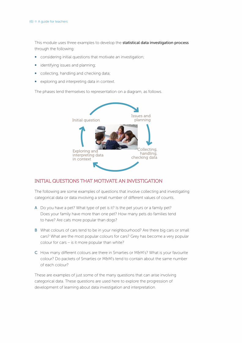
The phases lend themselves to representation on a diagram, as follows.

Initial question

Exploring and interpreting data in context

Issues and planning

Collecting, handling,

checking data

INITIAL QUESTIONS THAT MOTIVATE AN INVESTIGATION

The following are some examples of questions that involve collecting and investigating

categorical data or data involving a small number of different values of counts.

A Do you have a pet? What type of pet is it? Is the pet yours or a family pet?

Does your family have more than one pet? How many pets do families tend

to have? Are cats more popular than dogs?

B What colours of cars tend to be in your neighbourhood? Are there big cars or small

cars? What are the most popular colours for cars? Grey has become a very popular

colour for cars – is it more popular than white?

C How many different colours are there in Smarties or M&M’s? What is your favourite

colour? Do packets of Smarties or M&M’s tend to contain about the same number

of each colour?

These are examples of just some of the many questions that can arise involving

categorical data. These questions are used here to explore the progression of

development of learning about data investigation and interpretation.


General statistical notes for teachers

Identifying and describing categories

Categorical data are data in which each observation falls into one and only one category.

The categories are usually natural categories such as cat or dog, male or female, but often

there are many possible categories or different possible descriptions. If so, we need to

carefully choose our groupings and descriptions of them. Colour is usually categorical

unless we are being scientific and describing colour by a scientific measure. In Example C

above, the colours are chosen and fixed for us. However, in Example B, the investigators

will need to decide what colour groupings they are going to use and describe these

carefully so that the data collected are consistent and reliable. The description must also

be clear for anyone listening to, or reading, a report of the investigation.

Some categorical data need careful description of their categories. For example, period of

a day could be described as peak or off‑peak; day or night; morning, afternoon, evening,

night. A person’s age group could be described as child, teenager, adult. These examples

also illustrate that many sets of categorical data come from creating or imposing

categories for data such as time or age (which is itself time of course).


Count data

Each observation in a set of count data is a count value. Hence count data occur only

in situations such as observing the number of children in a family, the number of TV sets

owned by each family. Note that age does not a give count data because it has units

(years or months or weeks or days etc).

Some count data sets have many different observed values, such as number of people at

football matches collected over a season, but some have only a few different observed

values, such as number of dogs owned by city‑dwelling families. Count data with only

a few different observed values are often presented using the graphs developed for

categorical data.

IDENTIFYING ISSUES AND PLANNING

In this first part of the data investigative process, one or more questions or issues begin

the process of identifying the topic to be investigated. In thinking about how to investigate

these, other questions and ideas can tend to arise. Refining and sorting these questions

and ideas along with considering how we are going to obtain data that is needed to

investigate them, help our planning to take shape. A data investigation is planned through

the interaction of the questions:

• ‘What do we want to find out about?’

• ‘What data can we get?’ and

• ‘How do we get the data?’


EXAMPLE A: PETS

The general topic is investigating domestic or family pets. The questions above are just

some that may arise in a free discussion. On the surface, this topic may seem simple but

there are many aspects of it to be considered before a data investigation can be undertaken.

Some questions that need to be considered include, what sort of pets are we going to

consider, and are we going to consider pets of the families with a child in Year 4 at this

school, or are we going to consider more than just one class or one year level.

Students need to decide what can be called a pet even if they do not choose categories

before collecting the data. For example, they may decide that a pet must be a living

animal (so that pet rocks or inanimate pets are not considered) and that to be classified as

a pet, an animal must be fed by the family, housed in the precinct of the family home and

participate in some way with members of the family. Students living in rural or agricultural

areas may need to discuss this carefully before deciding what can be classified as a pet.

Another type of consideration that comes under both identifying the issues or questions

and in the planning, is on whom or what are we going to collect these data. The data

are most likely collected from students, whether restricted to one class or year level or

whether other classes or year levels are involved. Which ‘family’ to consider in the case of

dual families needs to be clear. If more than one class or year level provides information,

care will be needed to avoid double‑counting of families with siblings at the school.

Notice that by considering pets as belonging to families, we avoid the difficulty of what

would we mean by an individual student at this year level ‘owning’ a pet.

Next we need to consider what data we are going to collect. We could just ask for the

number of pets in total, or we could ask for numbers of different types of pets, or we

could simply ask for a listing of pets per family and then the students can decide how to

classify the pets once the data are collected. It is likely that students will be interested in

the various types of pets of the families of their classmates, so a listing of pets per family

may be the best raw data to collect.

EXAMPLE B: CARS

The general topic is colour of cars. As with pets, there are many aspects of this topic that

need discussion and decisions. The first is, what do we mean by a ‘car’? Are we going to

include all types of vehicles or not consider trucks, buses, motor bikes etc? This is up to

the students and their teacher – the important point is to make sure that those collecting

the data are clear about what to observe and that it is described clearly in any reporting.

We need to decide where we are going to collect the data. They could be collected by

observation of cars passing the school, or of cars parked in a large carpark, or by a survey

of students reporting the colour of the car or cars owned by their family. Only one of

these ways should be used to avoid doubling counting (or even triple counting!) and each

way may or may not represent slightly different general situations. This last point can be

raised even at such early stages of development.


Colour of cars is not straightforward, and, unlike the pet example, how to record

colours must be worked out before the data are collected in order to obtain consistent

data. Although there might be many opinions offered by students, at this early stage of

development, some simple classifications could be selected, such as: white; black; grey or

silver; all reds, yellows, browns; all blues, greens, purple.

EXAMPLE C: M&M’S OR SMARTIES

The general topic is colour of Smarties (or M&M’s). This is the simplest of the three

examples here from the point of view of what to observe. The same type of sweet would

be observed (e.g. not peanut ones) and the colours are set by the manufacturer. One

decision that is needed is what size packet to buy and whether to look at colours in each

packet with a number of different packets or whether just to look at one large number of

sweets. However comparing summaries of colours observed over different packets of the

same size provides an introduction to concepts of variation over samples – in this case,

samples of sweets. In this example, the colours could be recorded separately for each

packet and then the data could be combined overall.


Each of the above examples demonstrates key statistical aspects of the initial phases of

data investigations in illustrating

• how initial ideas lead to questions to be investigated which then lead to identification

of what is to be collected or observed

• identification of the ‘subjects’ – on what will the data be observed or collected

• early considerations of what the data represent.

Planning a statistical investigation involves identification of what is to be observed (what

data are we going to collect) and the ‘subjects’ or ‘experimental units’ of the investigation

– that is, on what are we are going to collect or observe our data?

The ‘what’ we are going to observe is called a statistical variable.

In Example B, the ‘subjects’ are cars, and the variable of interest is ‘colour of car’. We could

summarise our plan by the sentence, ‘The cars passing the school will be classified by

their colour’.

In Example C, the ‘subjects’ are individual sweets, and the variable of interest is colour

of the sweet. We could summarise our plan by the sentence, ‘Each sweet in a packet of

M&M’s will be classified by its colour’.


COLLECTING, HANDLING AND CHECKING DATA

EXAMPLE A: PETS

For the example on pets, if the data are collected by listing all pets, the recording form

might look like this:

STUDENT NAME FAMILY NAME PETS

Abigail Jones Dog, 2 birds

Fred Smith 2 mice, tortoise

Jenny Nguyen Cat

If the classifications of pets are chosen before the data are collected, the recording form

might look like this:

STUDENT NAME

FAMILY NAME DOGS CATS BIRDS OTHER

Abigail Jones 1 0 2 0

Fred Smith 0 0 0 3

Jenny Nguyen 0 1 0 0

From either form, the total number of pets for each family is readily obtained. If the data

are originally collected according to the first recording form above, then how to group the

data will need to be considered if it is wished to produce a table like the second above.

If the data are collected on the families of the students in the class(es) which discussed

the investigation, they will be aware of the decisions of what is a pet, and what is a family.

However, the students should express it in their own words for inclusion in reporting.

If the data are collected from other students or classes, the students collecting the data

need to have an agreed form of words when asking other students. A trial/rehearsal of this

is advisable for both confidence and consistency – and for fun!

Note that because of recording the student’s and family’s name, the number of pets of

families for boys and girls in Year 4 could be considered separately if a reasonably sized

dataset is collected.


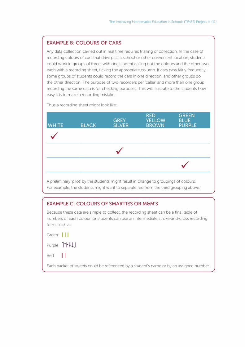
EXAMPLE B: COLOURS OF CARS

Any data collection carried out in real time requires trialling of collection. In the case of

recording colours of cars that drive past a school or other convenient location, students

could work in groups of three, with one student calling out the colours and the other two,

each with a recording sheet, ticking the appropriate column. If cars pass fairly frequently,

some groups of students could record the cars in one direction, and other groups do

the other direction. The purpose of two recorders per ‘caller’ and more than one group

recording the same data is for checking purposes. This will illustrate to the students how

easy it is to make a recording mistake.

Thus a recording sheet might look like:

WHITE BLACKGREY SILVER

RED YELLOW BROWN

GREEN BLUE PURPLE

A preliminary ‘pilot’ by the students might result in change to groupings of colours.

For example, the students might want to separate red from the third grouping above.

EXAMPLE C: COLOURS OF SMARTIES OR M&M’S

Because these data are simple to collect, the recording sheet can be a final table of

numbers of each colour, or students can use an intermediate stroke‑and‑cross recording

form, such as

Green

Purple

Red

Each packet of sweets could be referenced by a student’s name or by an assigned number.



The form of recording sheets tends to depend on the practicalities of the investigation.

Usually the rows of the recording sheet correspond to the ‘subjects’.

In Example A, the ‘subjects’ are families, identified by the child who is representing the

family. The second form of the recording sheet is recording the numbers of dogs, cats,

birds and ‘other’ pets for each family. From this, the total number of pets for each family

can be obtained.

In Example B, the ‘subjects’ are cars and each row of the recording sheet corresponds to

a car. There is only one variable, colour, but because it is difficult to write down a colour

or even a letter quickly, the recording sheet can be designed for convenience in quick

recording by just requiring a tick. If this was part of a larger investigation, the data collected

by the above recording sheet should be then converted to a sheet containing one column

that records the colour category by name.

In Example C, the ‘subjects’ are individual sweets. The raw data would be a single column

in which each sweet would be classified by its colour. Because this is tedious in this simple

situation, the stroke‑and‑cross method can be used to bypass the raw recording sheet to

go straight to obtaining the summary data.

EXPLORING AND INTERPRETING DATA

It is in exploring data that we use presentations, including graphical and

summary presentations.

Categorical data are summarised by the number of observations that fall in each category.

These are called the frequencies of the data – how often did each category occur. These

frequencies can be presented in a table or can be graphed by a column graph in which

each category has a column and the heights of the columns represent the frequency of

the observations that fall in that category.

Count data are also summarised by the number of observations that fall in each

category, where the categories correspond to the different possible count values that the

observations take.

Thus frequency of a category is the numbers of observations in the data that fall into that

category. It is frequencies that provide the information on how likely are the different

categories. A similar statement for values of counts can be made.

Column graphs are also called barcharts.



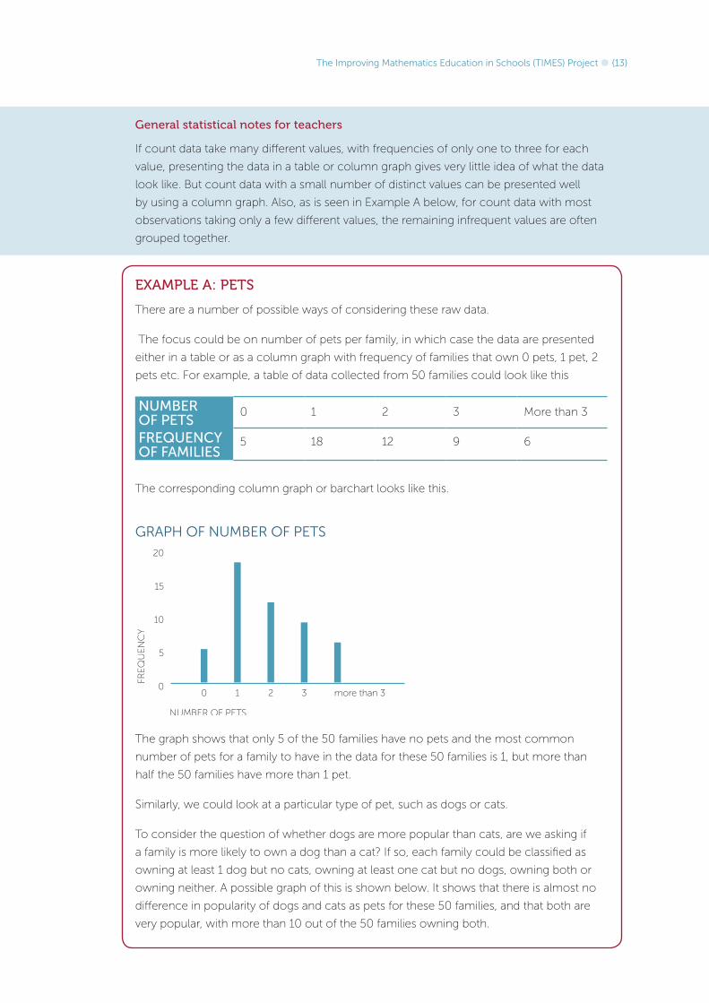
If count data take many different values, with frequencies of only one to three for each

value, presenting the data in a table or column graph gives very little idea of what the data

look like. But count data with a small number of distinct values can be presented well

by using a column graph. Also, as is seen in Example A below, for count data with most

observations taking only a few different values, the remaining infrequent values are often

grouped together.

EXAMPLE A: PETS

There are a number of possible ways of considering these raw data.

The focus could be on number of pets per family, in which case the data are presented

either in a table or as a column graph with frequency of families that own 0 pets, 1 pet, 2

pets etc. For example, a table of data collected from 50 families could look like this

NUMBER OF PETS

0 1 2 3 More than 3

FREQUENCY OF FAMILIES

5 18 12 9 6

The corresponding column graph or barchart looks like this.

GRAPH OF NUMBER OF PETS

FRE

QU

EN

CY

NUMBER OF PETS

20

15

10

5

0 1 2 3 more than 30

The graph shows that only 5 of the 50 families have no pets and the most common

number of pets for a family to have in the data for these 50 families is 1, but more than

half the 50 families have more than 1 pet.

Similarly, we could look at a particular type of pet, such as dogs or cats.

To consider the question of whether dogs are more popular than cats, are we asking if

a family is more likely to own a dog than a cat? If so, each family could be classified as

owning at least 1 dog but no cats, owning at least one cat but no dogs, owning both or

owning neither. A possible graph of this is shown below. It shows that there is almost no

difference in popularity of dogs and cats as pets for these 50 families, and that both are

very popular, with more than 10 out of the 50 families owning both.


GRAPH OF CAT OR DOGFR

EQ

UE

NC

Y

CAT OR DOG

16

18

14

10

12

4

6

8

2

both cat dog neither0

EXAMPLE B: COLOURS OF CARS

From the form of the recording sheets above, it is a simple matter to obtain the frequencies

of the different colours. Checks can then be made across recording sheets within each

group and across groups. Differences of one or two totals for each colour are probably not

worth checking, but if there are big differences, recording sheets can be compared.

GRAPH OF COLOUR OF CARS

FREQ

UE

NC

Y

COLOUR

BLACK BLUE GREEN

GRAY RED YELLOW BROWN

WHITE

40

30

20

10

0

A column graph of the car colours could look like the one shown above. This shows

that white is the most common colour in these data, closely followed by the group that

includes red, yellow, brown. Perhaps putting all those colours in one group was not a

good choice! The group of blues and greens is next but much less popular, and there

were very few black cars passing on that day.


EXAMPLE C: COLOURS OF SMARTIES OR M&M’S

As with the colours of cars, the numbers of sweets of each colour can be presented in

tables or column graphs. It is easily seen how valuable the column graphs are for ‘seeing’

what the data are like and, in an example like this, for comparing colour frequencies in

different packets of sweets. Below are column graphs of colours of M&M’s in 6 different

packets. Note that the scale of the column graphs is the same so that we can easily

compare the frequencies of colours within and across packets.

FRE

QU

EN

CY

PACKET 1

GRAPH OF PACKET 1

8

10

12

6

4

2

BROW

N

GREEN

ORANGE

RED

YELL

OW

BLUE

0 FRE

QU

EN

CY

PACKET 2

GRAPH OF PACKET 2

8

10

12

6

4

2

BROW

N

GREEN

ORANGE

RED

YELL

OW

BLUE

0

FREQ

UE

NC

Y

PACKET 3

GRAPH OF PACKET 3

8

10

12

6

4

2

BROW

N

GREEN

ORANGE

RED

YELL

OW

BLUE

0 FREQ

UE

NC

Y

PACKET 4

GRAPH OF PACKET 4

8

10

12

6

4

2

BROW

N

GREEN

ORANGE

RED

YELL

OW

BLUE

0

FREQ

UE

NC

Y

PACKET 5

GRAPH OF PACKET 5

8

10

12

6

4

2

BROW

N

GREEN

ORANGE

RED

YELL

OW

BLUE

0 FREQ

UE

NC

Y

PACKET 6

GRAPH OF PACKET 6

8

10

12

6

4

2

BROW

N

GREEN

ORANGE

RED

YELL

OW

BLUE

0

These graphs demonstrate well the amount of variation in frequencies of colours there

can be across packets, even if overall the manufacturers use a fixed set of proportions of

colours. [Aside: in this example, the overall fixed percentages of the different colours from

which these data were obtained was: 24% blue; 14% brown; 16% green; 20% orange; 13%

red; 14% yellow.]


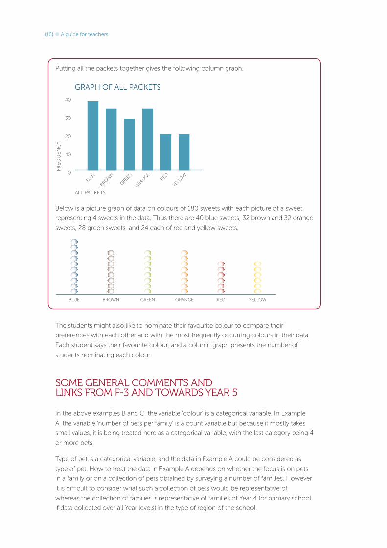
Putting all the packets together gives the following column graph.

FREQ

UE

NC

Y

ALL PACKETS

GRAPH OF ALL PACKETS

10

20

30

40

BROW

N

GREEN

ORANGE

RED

YELL

OW

BLUE0

Below is a picture graph of data on colours of 180 sweets with each picture of a sweet

representing 4 sweets in the data. Thus there are 40 blue sweets, 32 brown and 32 orange

sweets, 28 green sweets, and 24 each of red and yellow sweets.

BROWN GREEN ORANGE RED YELLOWBLUE

The students might also like to nominate their favourite colour to compare their

preferences with each other and with the most frequently occurring colours in their data.

Each student says their favourite colour, and a column graph presents the number of

students nominating each colour.

SOME GENERAL COMMENTS AND LINKS FROM F-3 AND TOWARDS YEAR 5

In the above examples B and C, the variable ‘colour’ is a categorical variable. In Example

A, the variable ‘number of pets per family’ is a count variable but because it mostly takes

small values, it is being treated here as a categorical variable, with the last category being 4

or more pets.

Type of pet is a categorical variable, and the data in Example A could be considered as

type of pet. How to treat the data in Example A depends on whether the focus is on pets

in a family or on a collection of pets obtained by surveying a number of families. However

it is difficult to consider what such a collection of pets would be representative of,

whereas the collection of families is representative of families of Year 4 (or primary school

if data collected over all Year levels) in the type of region of the school.


Although simple categorical data are used in Years F‑3, the above material marks the

first experiences in the process of statistical data investigations. The focus has been on

considering just one categorical variable at a time, so that the only types of presentations

are tables and column graphs with just one set of categories. In this relatively simple

situation the above examples illustrate the extent of statistical thinking involved in the initial

stages of an investigation in identifying the questions/issues and in planning and collecting

the data.

The three examples of the module can demonstrate concepts such as ‘what do our data

represent’ and variation in data across samples. Variation in data across samples tends

to arise naturally in everyday situations that are very familiar to young students. These

concepts are further developed as students progress.

In Year 5, we extend the concepts of types of data to consider measurement data and

more general situations with count data. In Year 5, although questions and issues may

involve more than one variable, the focus is on exploring and interpreting phases of the

investigation process with one variable at a time.

The aim of the International Centre of Excellence for

Education in Mathematics (ICE‑EM) is to strengthen

education in the mathematical sciences at all levels‑

from school to advanced research and contemporary

applications in industry and commerce.

ICE‑EM is the education division of the Australian

Mathematical Sciences Institute, a consortium of

27 university mathematics departments, CSIRO

Mathematical and Information Sciences, the Australian

Bureau of Statistics, the Australian Mathematical Society

and the Australian Mathematics Trust.

www.amsi.org.au

The ICE‑EM modules are part of The Improving

Mathematics Education in Schools (TIMES) Project.

The modules are organised under the strand

titles of the Australian Curriculum:

• Number and Algebra

• Measurement and Geometry

• Statistics and Probability

The modules are written for teachers. Each module

contains a discussion of a component of the

mathematics curriculum up to the end of Year 10.

Documents

STATISTICS AND DATA INVESTIGATION AND INTERPRETATION … · where each observation falls into one of a number ... learning about data investigation and interpretation. ... be considered