Embed Size (px)
Citation preview
Statistics and Quantitative Analysis U4320
Segment 10 Prof. Sharyn O’Halloran
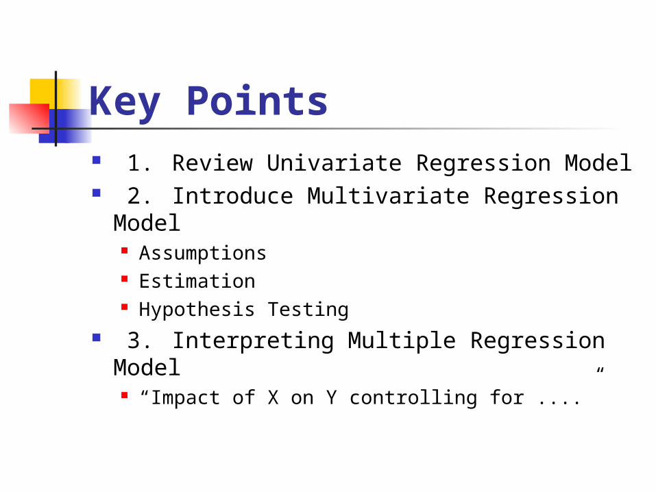
Key Points 1. Review Univariate Regression Model 2. Introduce Multivariate Regression
Model Assumptions Estimation Hypothesis Testing
3. Interpreting Multiple Regression Model “Impact of X on Y controlling for ....”
I. Univariate Analysis
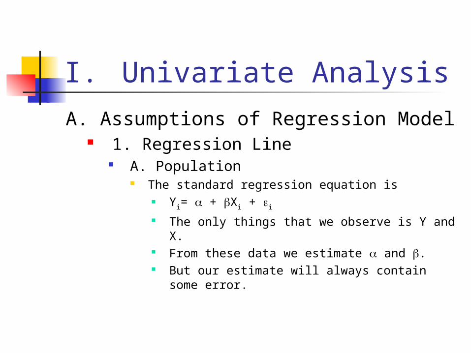
A. Assumptions of Regression Model 1. Regression Line
A. Population The standard regression equation is
Yi= + Xi + i The only things that we observe is Y and
X. From these data we estimate and . But our estimate will always contain
some error.
Univariate Analysis (cont.)
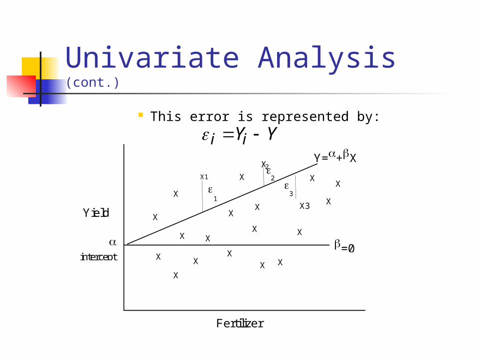
This error is represented by: i iY Y
Fertilizer
Yield
intercept
=0
Y=+X
X
X
X
X
X
X
X
X
X
X X
X
X1
X3
X
X X
X
X
XX
2
1
3
2
Univariate Analysis (cont.)
B. Sample Most times we don’t observe the underlying
population parameters. All we observe is a sample of X and Y values
from which make estimates of and .
Univariate Analysis (cont.)
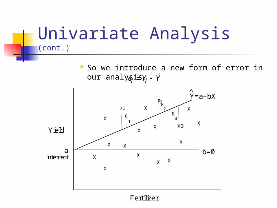
So we introduce a new form of error in our analysis. e Y Yi i
Fertilizer
Yield
aintercept
b=0
Y=a+bX
X
X
X
X
X
X
X
X
X
X
X1
X3
X
X
X
X
X
2
1
3
2
Univariate Analysis (cont.)
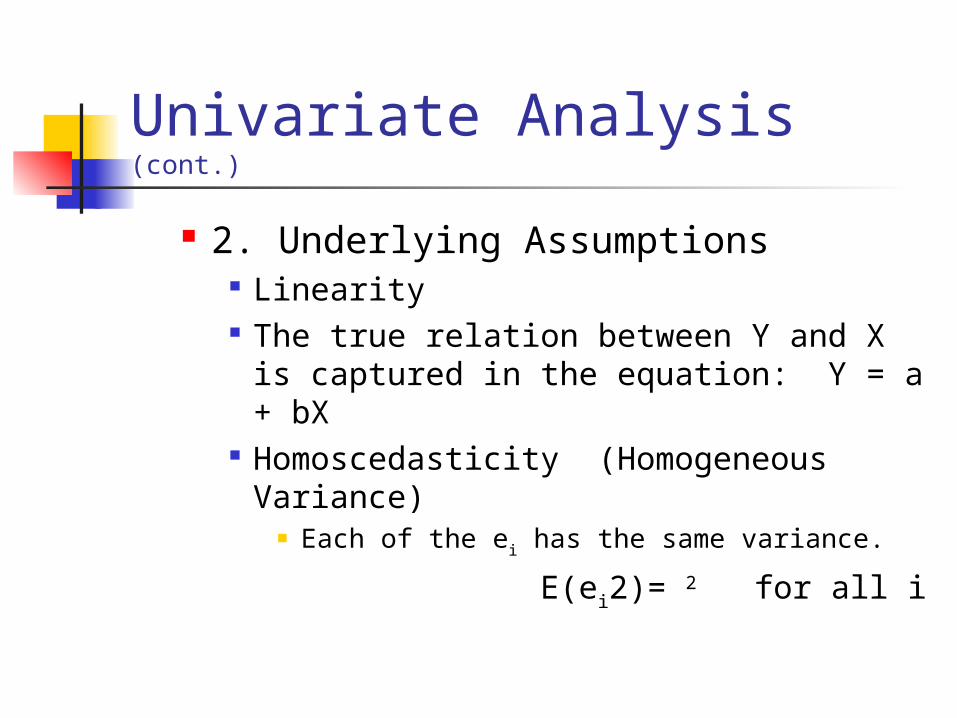
2. Underlying Assumptions Linearity The true relation between Y and X is
captured in the equation: Y = a + bX Homoscedasticity (Homogeneous
Variance) Each of the ei has the same variance.
E(ei2)= 2 for all i
Univariate Analysis (cont.)
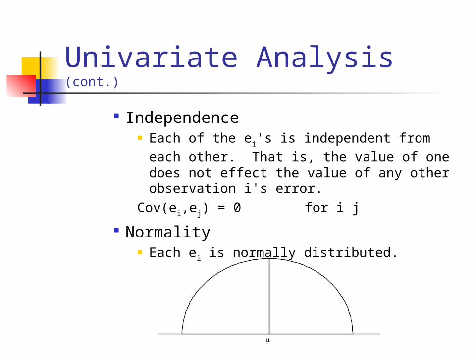
Independence Each of the ei's is independent from each
other. That is, the value of one does not effect the value of any other observation i's error.
Cov(ei,ej) = 0 for i j
Normality Each ei is normally distributed.
Univariate Analysis (cont.)
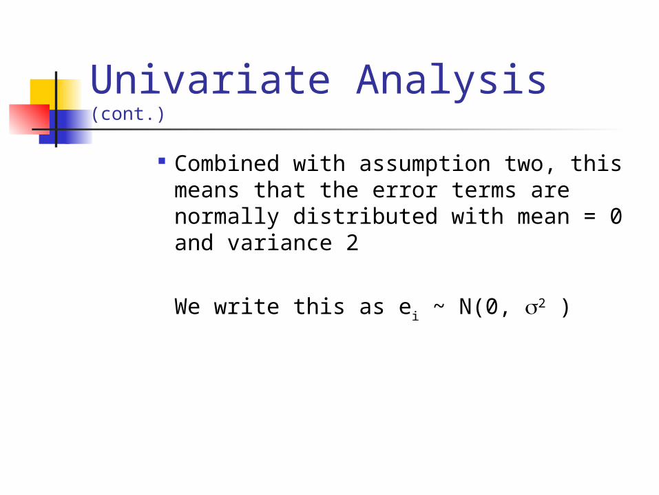
Combined with assumption two, this means that the error terms are normally distributed with mean = 0 and variance 2
We write this as ei ~ N(0, 2 )
Univariate Analysis (cont.)
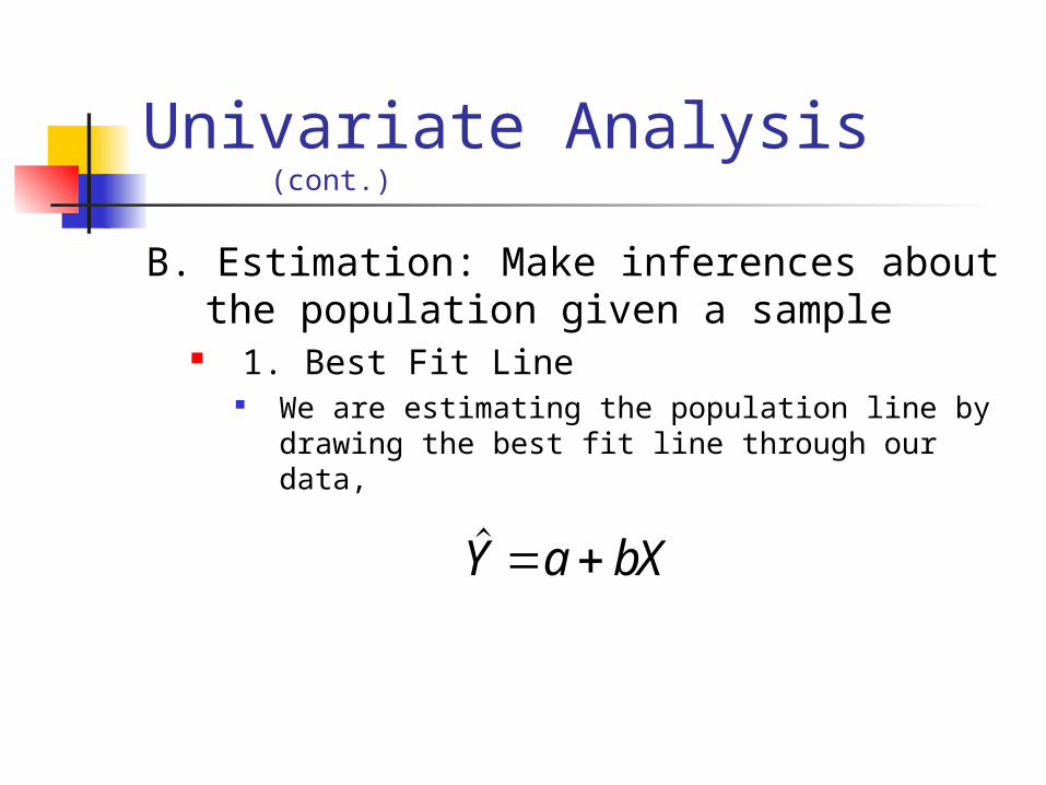
B. Estimation: Make inferences about the population given a sample
1. Best Fit Line We are estimating the population line by
drawing the best fit line through our data,
Y a bX
Univariate Analysis (cont.)
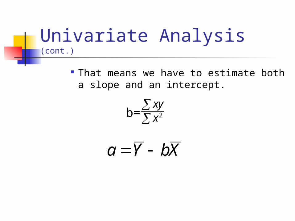
That means we have to estimate both a slope and an intercept.
xyx
2b=
a Y bX
Univariate Analysis (cont.)
Usually, we are interested in the slope. Why?
Testing to see if the slope is not equal to zero is testing to see if one variable has any influence on the other.
Univariate Analysis (cont.)
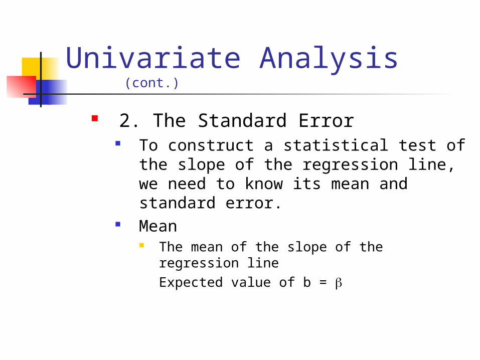
2. The Standard Error To construct a statistical test of the
slope of the regression line, we need to know its mean and standard error.
Mean The mean of the slope of the regression line
Expected value of b =
Univariate Analysis (cont.)
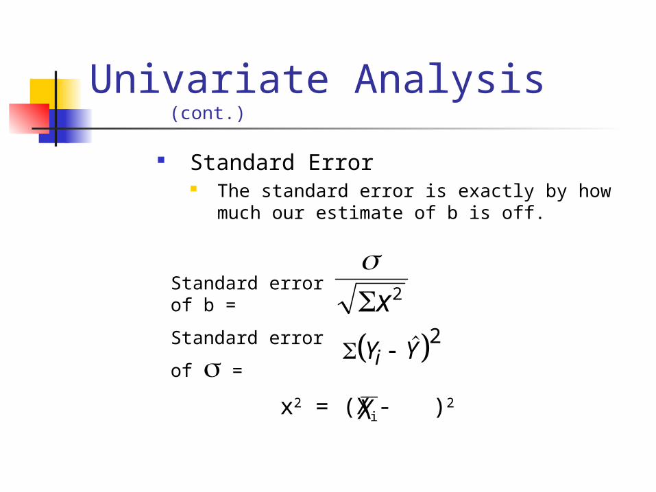
Standard Error The standard error is exactly by how much
our estimate of b is off.
x2
Y Yi 2
Standard error of b =
Standard error of =
x2 = (Xi- )2 X
Univariate Analysis (cont.)
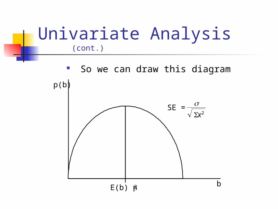
So we can draw this diagram
E(b) =
SE = x2
p(b)
b
Univariate Analysis (cont.)
This makes sense, b is the factor that relates the Xs to the Y, and the standard error depends on both which is the expected variations in the Ys and on the variation in the Xs.
Univariate Analysis (cont.)
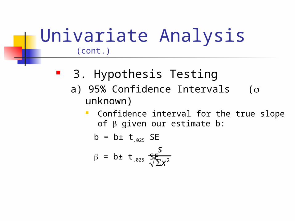
3. Hypothesis Testing a) 95% Confidence Intervals ( unknown)
Confidence interval for the true slope of given our estimate b:
s
x 2 = b± t.025 SE
b = b± t.025 SE
Univariate Analysis (cont.)
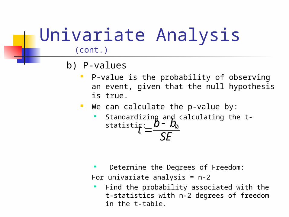
b) P-values P-value is the probability of observing an
event, given that the null hypothesis is true. We can calculate the p-value by:
Standardizing and calculating the t-statistic:
Determine the Degrees of Freedom: For univariate analysis =
n-2 Find the probability associated with the t-
statistics with n-2 degrees of freedom in the t-table.
tb bSE
0
Univariate Analysis (cont.)
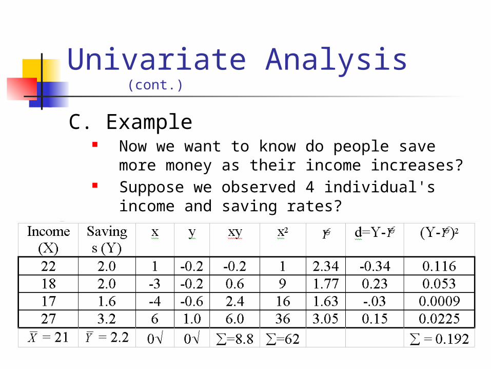
C. Example Now we want to know do people save
more money as their income increases? Suppose we observed 4 individual's
income and saving rates?
Univariate Analysis (cont.)
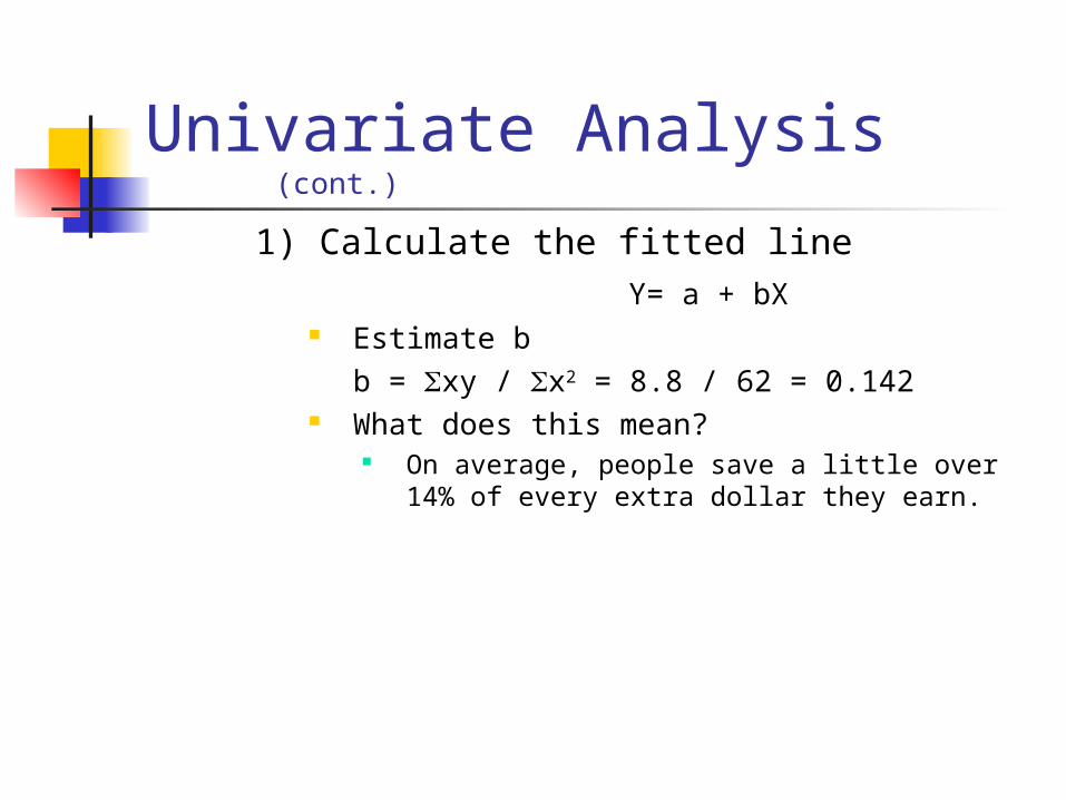
1) Calculate the fitted lineY= a + bX
Estimate bb = xy / x2 = 8.8 / 62 = 0.142
What does this mean? On average, people save a little over 14% of
every extra dollar they earn.
Univariate Analysis (cont.)
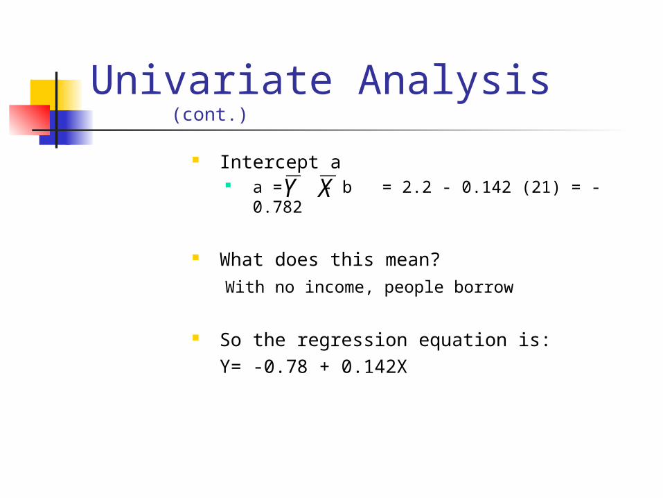
Intercept a a = - b = 2.2 - 0.142 (21) = -0.782
What does this mean? With no income, people borrow
So the regression equation is: Y= -0.78 + 0.142X
Y X
Univariate Analysis (cont.)
2) Calculate a 95% confidence interval Now let's test the null hypothesis that = 0.
That is, the hypothesis that people do not tend to save any of the extra money they earn.
H0: = 0 Ha: 0;
at the 5% significance level
Univariate Analysis (cont.)
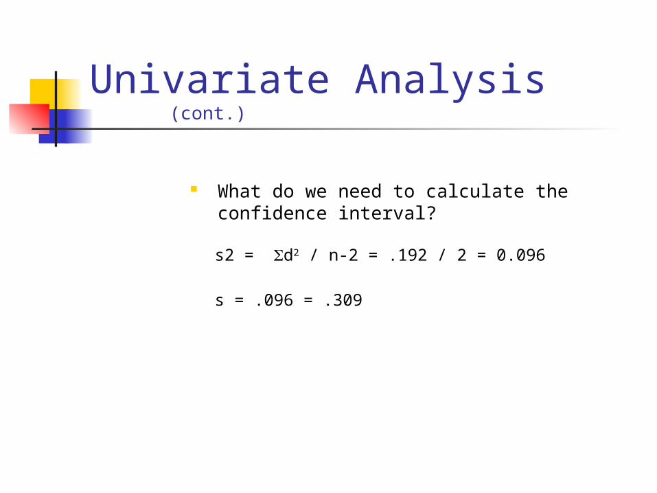
What do we need to calculate the confidence interval?
s2 = d2 / n-2 = .192 / 2 = 0.096
s = .096 = .309
Univariate Analysis (cont.)
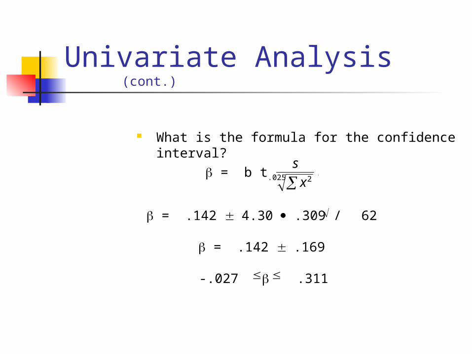
What is the formula for the confidence interval?
s
x2. = b t.025
= .142 4.30 .309 /62
= .142 .169
-.027 .311
Univariate Analysis (cont.)
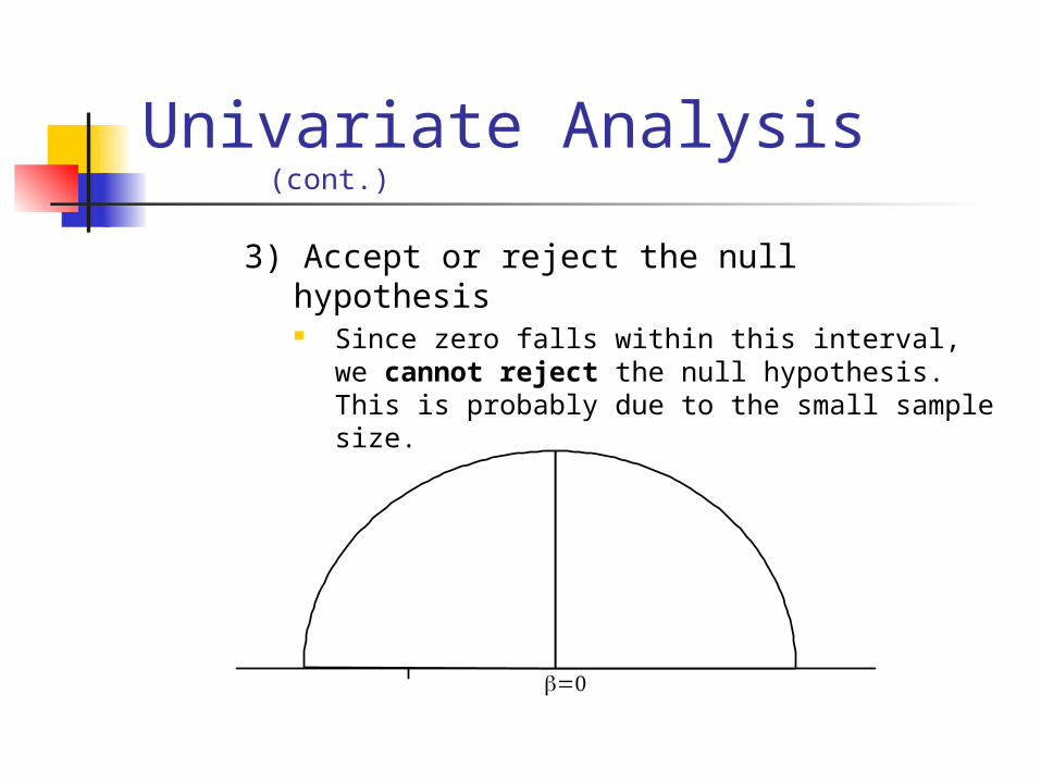
3) Accept or reject the null hypothesis Since zero falls within this interval, we
cannot reject the null hypothesis. This is probably due to the small sample size.
-.027 .311
Univariate Analysis (cont.)
D. Additional Examples 1. How about the hypothesis that = .50,
so that people save half their extra income?
It is outside the confidence interval, so we can reject this hypothesis
Univariate Analysis (cont.)
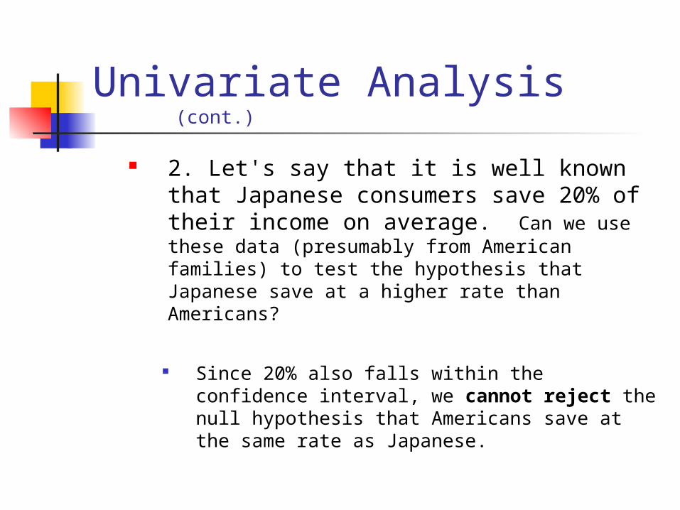
2. Let's say that it is well known that Japanese consumers save 20% of their income on average. Can we use these data (presumably from American families) to test the hypothesis that Japanese save at a higher rate than Americans?
Since 20% also falls within the confidence interval, we cannot reject the null hypothesis that Americans save at the same rate as Japanese.
II. Multiple Regression
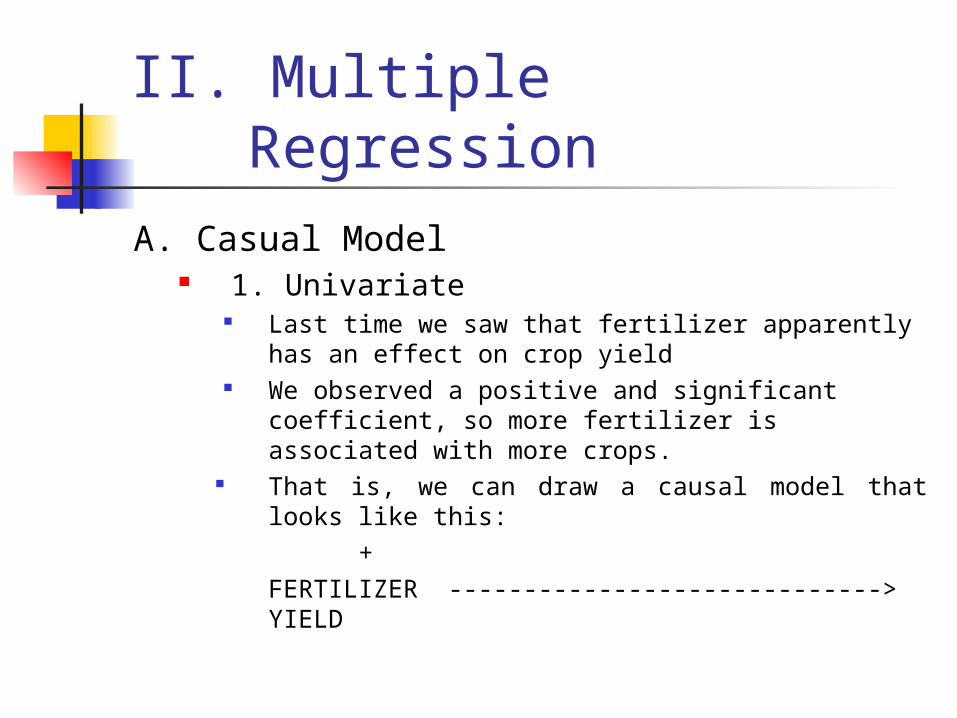
A. Casual Model 1. Univariate
Last time we saw that fertilizer apparently has an effect on crop yield
We observed a positive and significant coefficient, so more fertilizer is associated with more crops.
That is, we can draw a causal model that looks like this:
+FERTILIZER -----------------------------> YIELD
Multiple Regression (cont.)
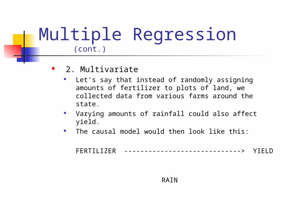
2. Multivariate Let's say that instead of randomly assigning
amounts of fertilizer to plots of land, we collected data from various farms around the state.
Varying amounts of rainfall could also affect yield.
The causal model would then look like this:
FERTILIZER -----------------------------> YIELD
RAIN
Multiple Regression (cont.)
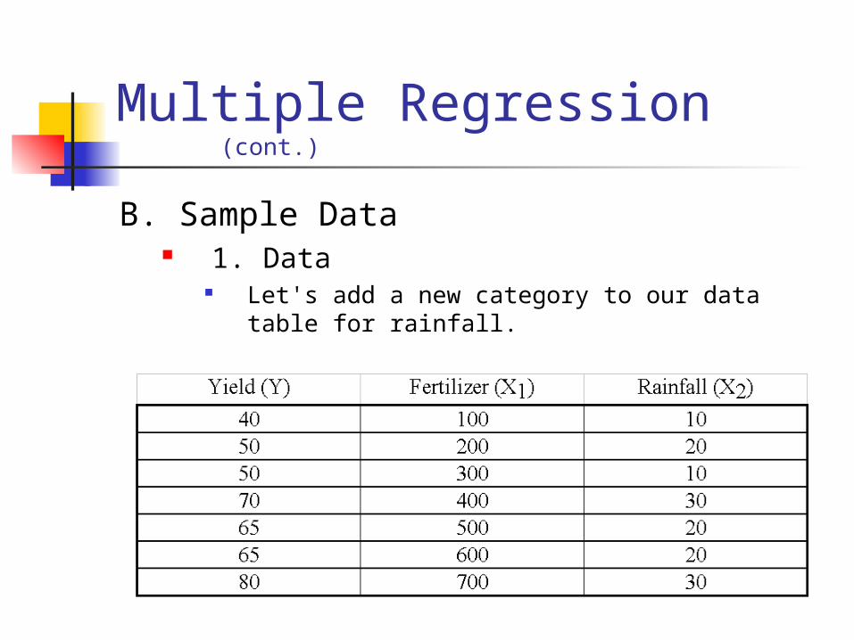
B. Sample Data 1. Data
Let's add a new category to our data table for rainfall.
Multiple Regression (cont.)
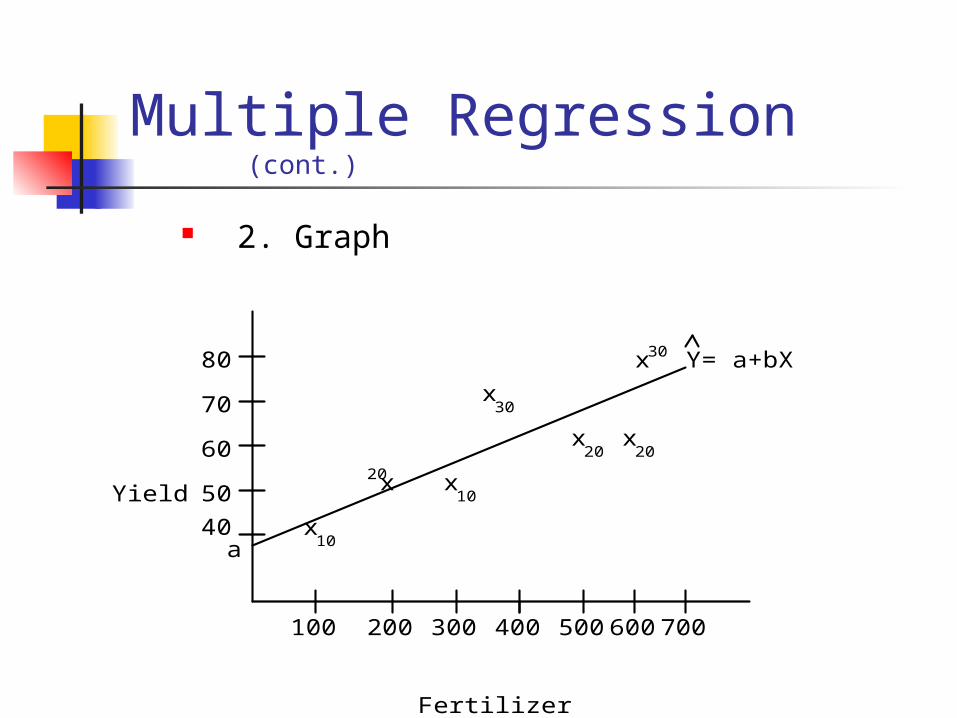
2. Graph
Yield
Fertilizer
40
50
60
70
80
100 200 300 400 500 600 700
x
x x
x
x x
x
a 10
20
10
20
20
30
30 Y= a+bX
Multiple Regression (cont.)
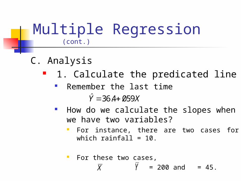
C. Analysis 1. Calculate the predicated line
Remember the last time
How do we calculate the slopes when we have two variables? For instance, there are two cases for which
rainfall = 10.
For these two cases, = 200 and = 45.
. .Y X 36 4 059
X Y
Multiple Regression (cont.)
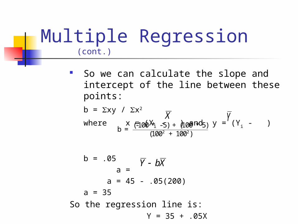
So we can calculate the slope and intercept of the line between these points:
b = xy / x2
where x = (Xi - ) and y = (Yi - )
b = .05 a = a = 45 - .05(200)
a = 35
So the regression line is:Y = 35 + .05X
b = (-100 * - 5) + (100 * 5)
(100 + 100 ) 2 2
Y bX
X Y
Multiple Regression (cont.)
Yield
Fertilizer
40
50
60
70
80
100 200 300 400 500 600 700
x
x x
x
x x
x
a 10
20
10
20
20
30
30
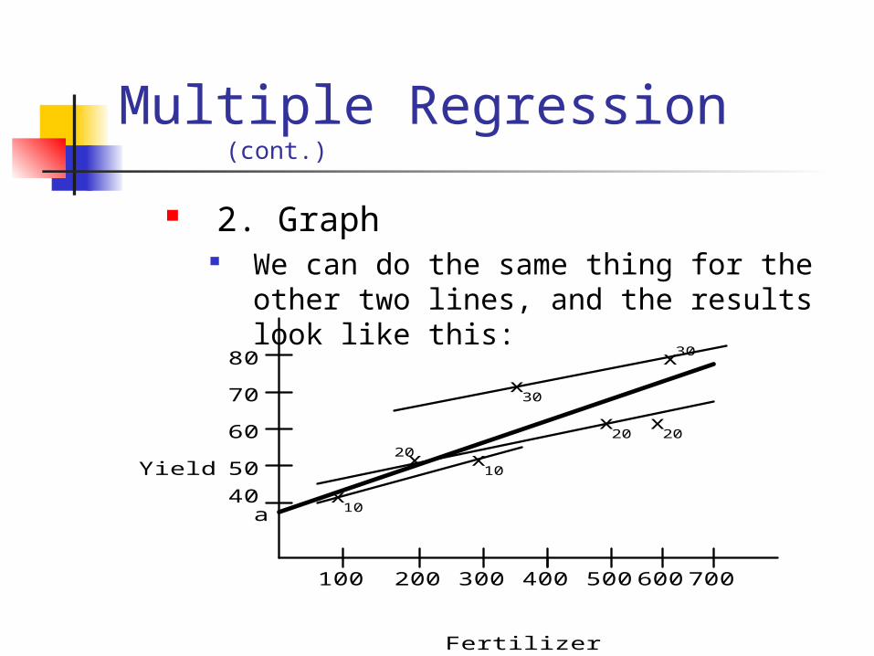
2. Graph We can do the same thing for the other
two lines, and the results look like this:
Multiple Regression (cont.)
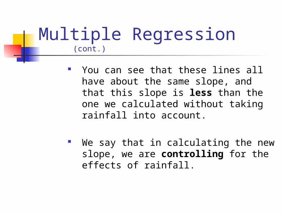
You can see that these lines all have about the same slope, and that this slope is less than the one we calculated without taking rainfall into account.
We say that in calculating the new slope, we are controlling for the effects of rainfall.
Multiple Regression (cont.)
3. Interpretation When rainfall is taken into account,
fertilizer is not as significant a factor as it appeared before.
One way to look at these results is that we can gain more accuracy by incorporating extra variables into our analysis.
III. Multiple Regression Model and OLS Fit
A. General Linear Model 1. Linear Expression
We saw that fertilizer apparently has an We write the equation for a regression line with two independent variables like this:
Y = 0 + 1X1 + 2X2.
Multiple Regression Model and OLS Fit (cont.)
Intercept Here, the y-intercept (or constant term) is
represented by b0.
How would you interpret 0?
0 is the level of the dependent variable when both independent variables are set to zero.
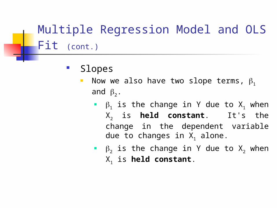
Slopes Now we also have two slope terms, 1 and 2.
1 is the change in Y due to X1 when X2 is held constant. It's the change in the dependent variable due to changes in X1 alone.
2 is the change in Y due to X2 when X1 is held constant.
Multiple Regression Model and OLS Fit (cont.)
Multiple Regression Model and OLS Fit (cont.)
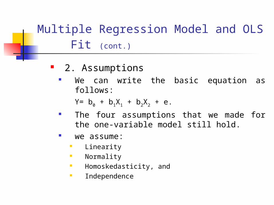
2. Assumptions We can write the basic equation as follows:
Y= b0 + b1X1 + b2X2 + e.
The four assumptions that we made for the one-variable model still hold.
we assume: Linearity Normality Homoskedasticity, and Independence
Multiple Regression Model and OLS Fit (cont.)
You can see that we can extend this type of equation as far as we'd like. We can just write:
Y = b0 + b1X1 + b2X2 + b3X3 + ... + e.
Multiple Regression Model and OLS Fit (cont.)
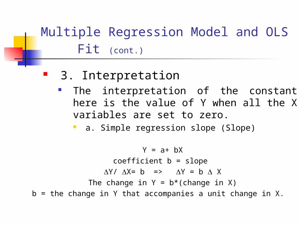
3. Interpretation The interpretation of the constant here is
the value of Y when all the X variables are set to zero. a. Simple regression slope (Slope)
Y = a+ bXcoefficient b = slope
Y/ X= b => Y = b XThe change in Y = b*(change in X)
b = the change in Y that accompanies a unit change in X.
Multiple Regression Model and OLS Fit (cont.)
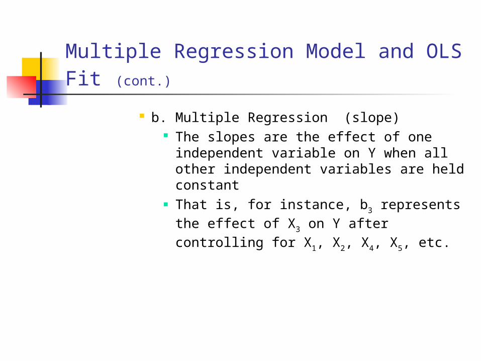
b. Multiple Regression (slope) The slopes are the effect of one
independent variable on Y when all other independent variables are held constant
That is, for instance, b3 represents the effect of X3 on Y after controlling for X1, X2, X4, X5, etc.
Multiple Regression Model and OLS Fit (cont.)
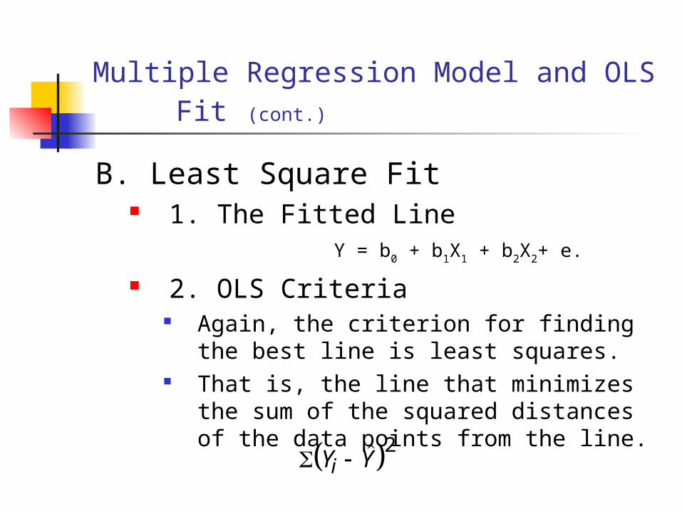
B. Least Square Fit 1. The Fitted Line
Y = b0 + b1X1 + b2X2+ e.
2. OLS Criteria Again, the criterion for finding the best
line is least squares. That is, the line that minimizes the sum
of the squared distances of the data points from the line.
Y Yi 2
Multiple Regression Model and OLS Fit (cont.)
3. Benefits of Multiple Regression
Reduce the sum of the squared residuals.
Adding more variables always improves the fit of your model.
Multiple Regression Model and OLS Fit (cont.)
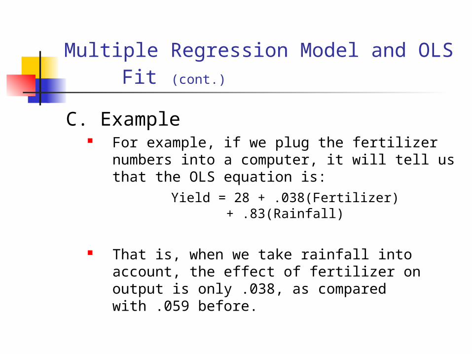
C. Example For example, if we plug the fertilizer
numbers into a computer, it will tell us that the OLS equation is:
Yield = 28 + .038(Fertilizer) + .83(Rainfall)
That is, when we take rainfall into account, the effect of fertilizer on output is only .038, as compared with .059 before.
IV. Confidence Intervals and Statistical Tests
Question: Does fertilizer still have a significant effect on yield, after controlling for
rainfall?
Confidence Intervals and Statistical Tests (cont.)
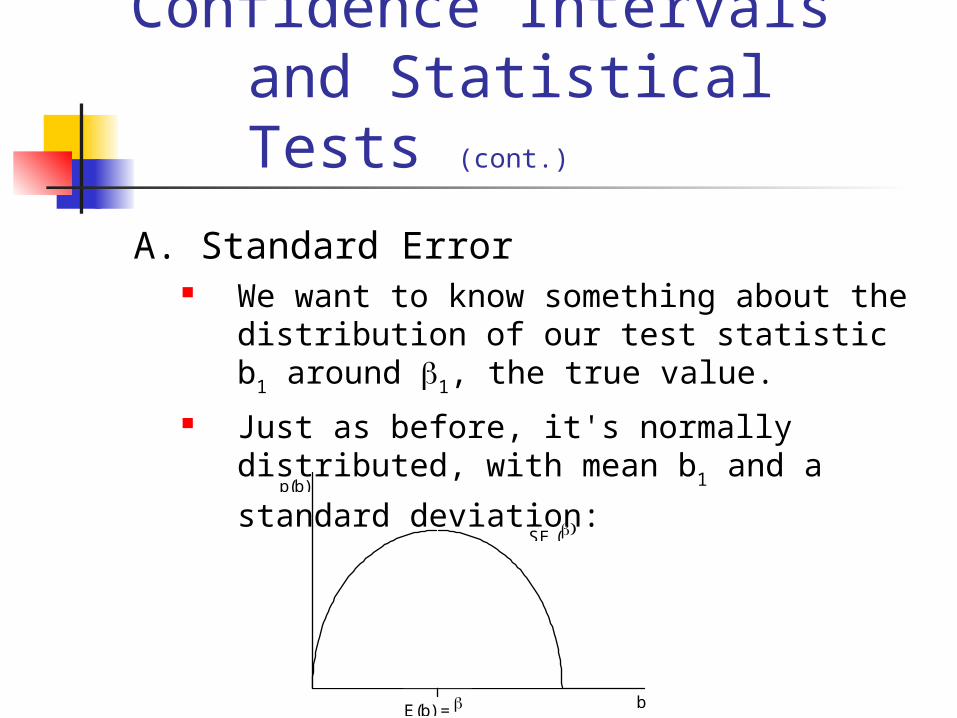
A. Standard Error We want to know something about the
distribution of our test statistic b1 around 1, the true value.
Just as before, it's normally distributed, with mean b1 and a standard deviation:
E(b) =
SE (
p(b)
b
Confidence Intervals and Statistical Tests (cont.)
B. Confidence Intervals and P-Values Now that we have a standard deviation for
b1, what can we calculate? That's right, we can calculate a
confidence interval for b1.
Confidence Intervals and Statistical Tests (cont.)
1. Formulas
Confidence IntervalCI (1) = b1 t.025 * SEb1
Confidence Intervals and Statistical Tests (cont.)
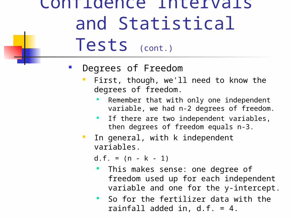
Degrees of Freedom First, though, we'll need to know the degrees
of freedom. Remember that with only one independent
variable, we had n-2 degrees of freedom. If there are two independent variables, then
degrees of freedom equals n-3. In general, with k independent variables.
d.f. = (n - k - 1) This makes sense: one degree of freedom
used up for each independent variable and one for the y-intercept.
So for the fertilizer data with the rainfall added in, d.f. = 4.
Confidence Intervals and Statistical Tests (cont.)
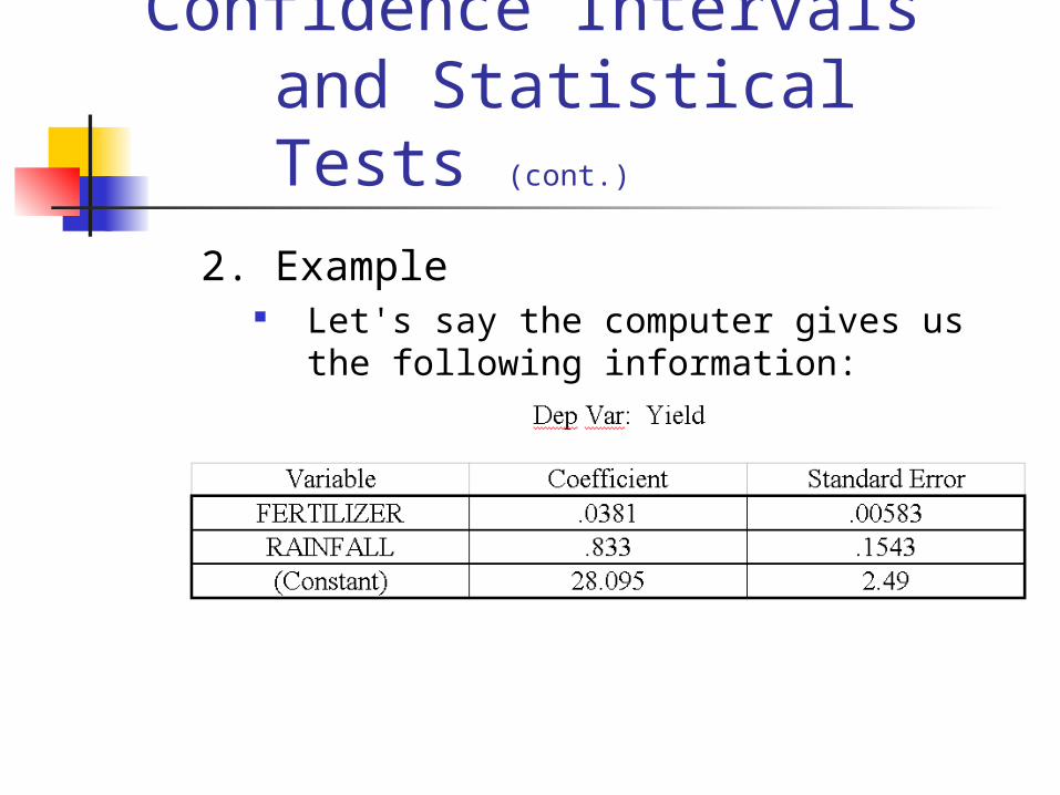
2. Example Let's say the computer gives us the
following information:
Confidence Intervals and Statistical Tests (cont.)
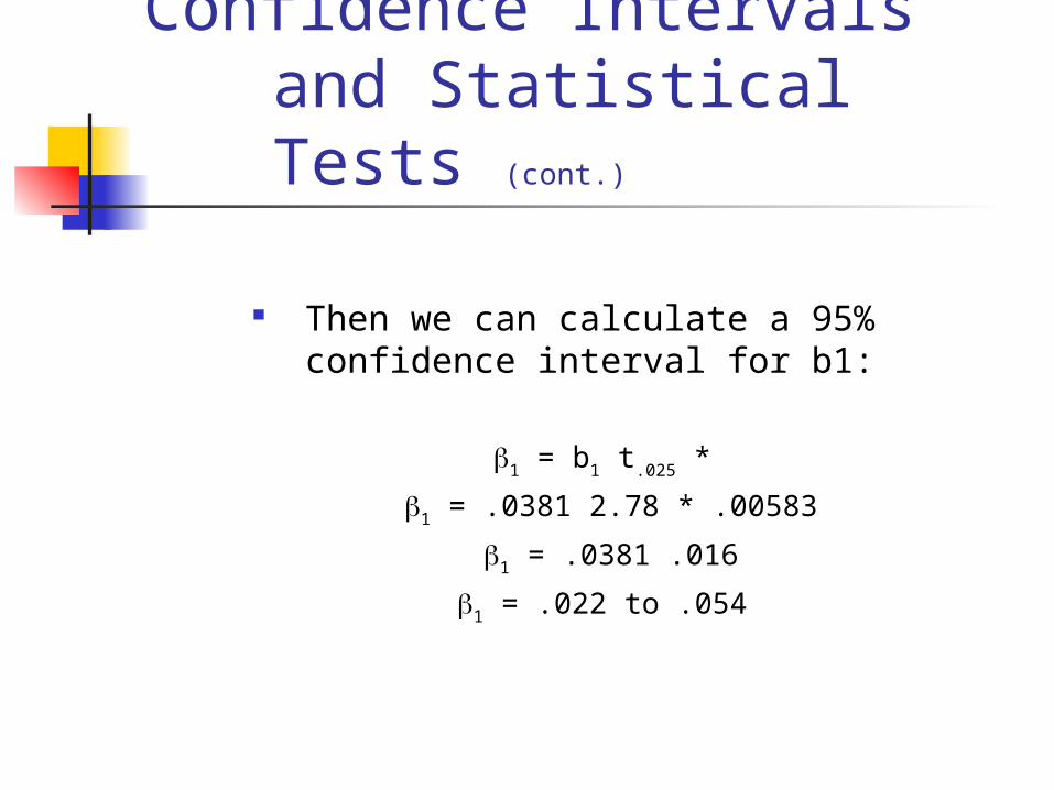
Then we can calculate a 95% confidence interval for b1:
1 = b1 t.025 *
1 = .0381 2.78 * .00583
1 = .0381 .016
1 = .022 to .054
Confidence Intervals and Statistical Tests (cont.)
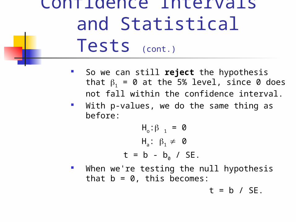
So we can still reject the hypothesis that 1 = 0 at the 5% level, since 0 does not fall within the confidence interval.
With p-values, we do the same thing as before: Ho: 1 = 0
Ha: 1 0
t = b - b0 / SE. When we're testing the null hypothesis that b =
0, this becomes: t = b / SE.
Confidence Intervals and Statistical Tests (cont.)
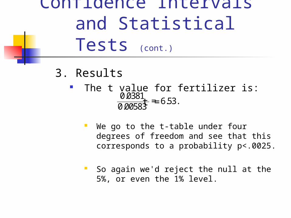
3. Results The t value for fertilizer is:
t =
We go to the t-table under four degrees of freedom and see that this corresponds to a probability p<.0025.
So again we'd reject the null at the 5%, or even the 1% level.
0.0381 0.00583
= 6.53.
Confidence Intervals and Statistical Tests (cont.)
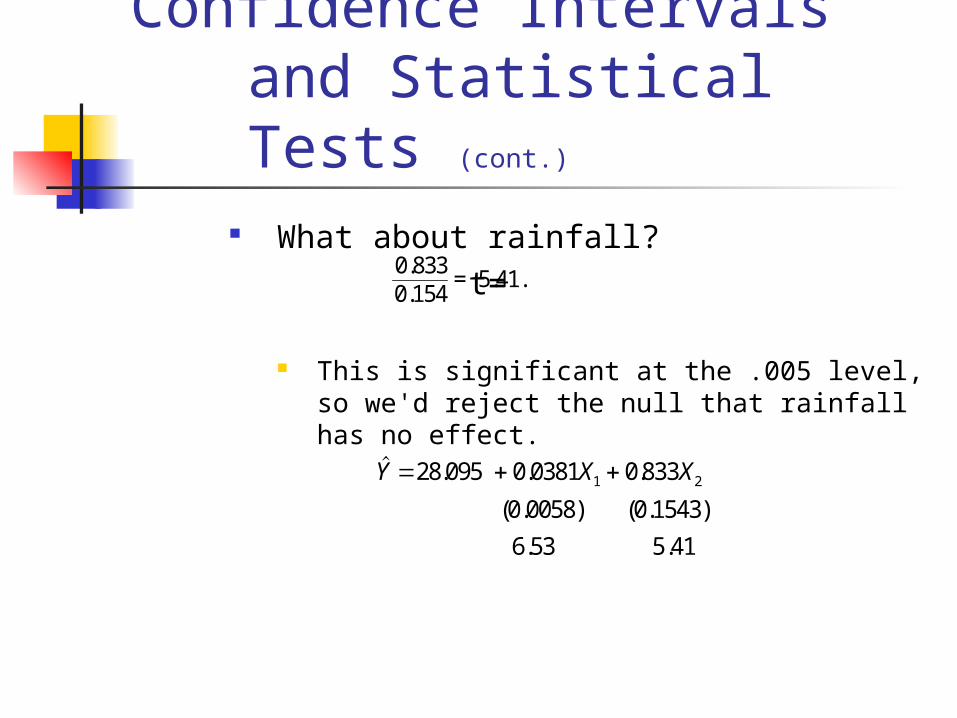
What about rainfall? t=
This is significant at the .005 level, so we'd reject the null that rainfall has no effect.
0.8330.154
= 5.41.
. . .Y X X 28 095 0 0381 0 8331 2
(0.0058) (0.1543)
6.53 5.41
Confidence Intervals and Statistical Tests (cont.)
C. Regression Results in Practice 1. Campaign Spending
The first analyzes the percentage of votes that incumbent congressmen received in 1984 (Dep. Var). The independent variables include: 1. the percentage of people registered in the same party in the district, 2. Voter approval of Reagan, 3. their expectations about their economic future, 4. challenger spending, and 5. incumbent spending.
The estimated coefficients are shown, with the standard errors in parentheses underneath.
Confidence Intervals and Statistical Tests (cont.)
2. Obscenity Cases The Dependent Variable is the probability that an
appeals court decided "liberally" in an obscenity case. The independent variables include:
1. Whether the case came from the South (this is Region)2. who appointed the justice, 3. whether the case was heard before or after the landmark 1973 Miller case, 4. who the accused person was, 5. what type of defense the defendant offered, and 6. what type of materials were involved in the case.
V. Homework
A. Introduction In your homework, you are asked to add
another variable to the regression that you ran for today's assignment. Then you are to find which coefficients are significant and interpret your results.
Homework (cont.)
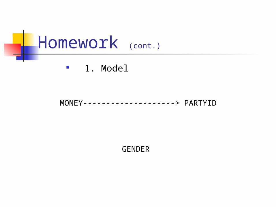
1. Model
MONEY--------------------> PARTYID
GENDER
Homework (cont.)
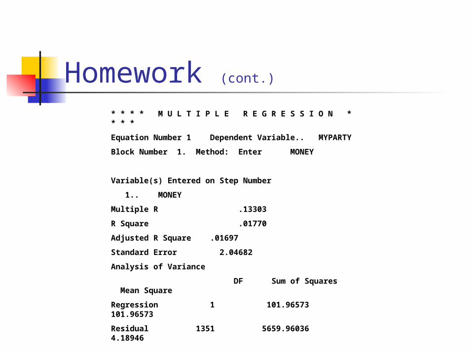
* * * * M U L T I P L E R E G R E S S I O N * * * *
Equation Number 1 Dependent Variable.. MYPARTY
Block Number 1. Method: Enter MONEY
Variable(s) Entered on Step Number
1.. MONEY
Multiple R .13303
R Square .01770
Adjusted R Square .01697
Standard Error 2.04682
Analysis of Variance
DF Sum of Squares Mean Square
Regression 1 101.96573 101.96573
Residual 1351 5659.96036 4.18946
F = 24.33863 Signif F = .0000
Homework (cont.)
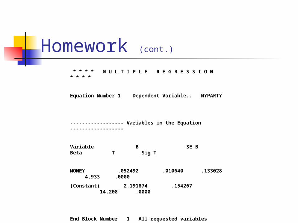
* * * * M U L T I P L E R E G R E S S I O N * * * *
Equation Number 1 Dependent Variable.. MYPARTY
------------------ Variables in the Equation ------------------
Variable B SE B Beta T Sig T
MONEY .052492 .010640 .133028 4.933 .0000
(Constant) 2.191874 .154267 14.208 .0000
End Block Number 1 All requested variables entered.
Homework (cont.)
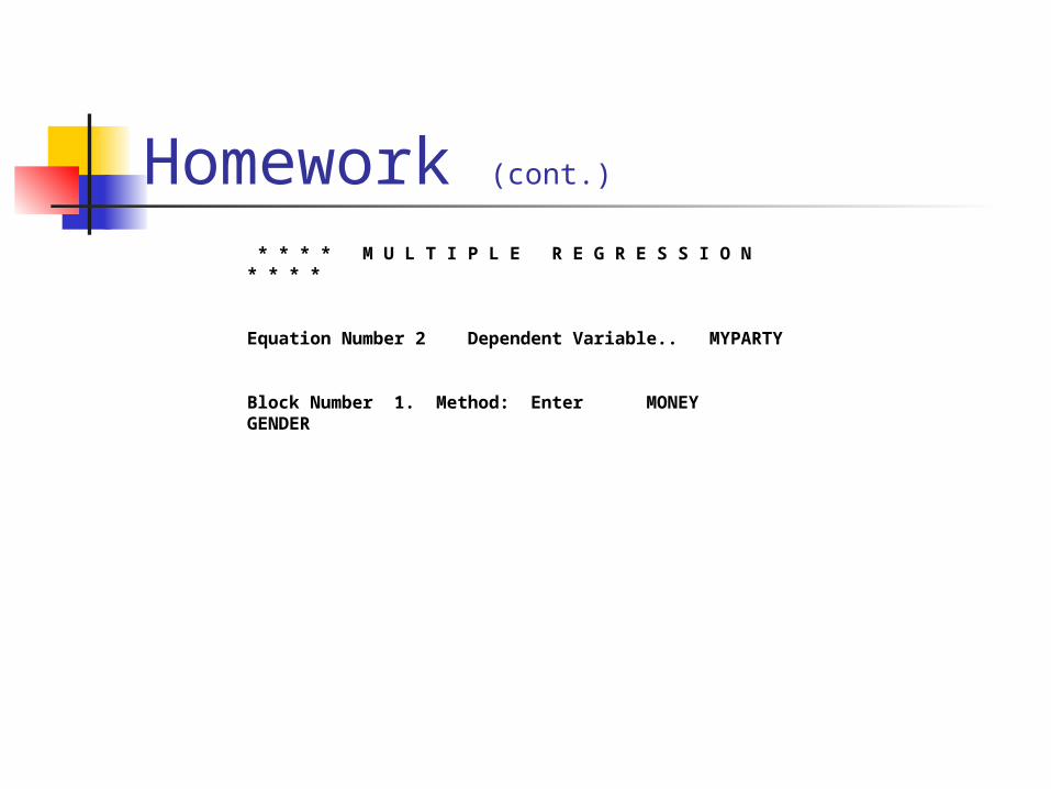
* * * * M U L T I P L E R E G R E S S I O N * * * *
Equation Number 2 Dependent Variable.. MYPARTY
Block Number 1. Method: Enter MONEY GENDER
Homework (cont.)
* * * * M U L T I P L E R E G R E S S I O N * * * *
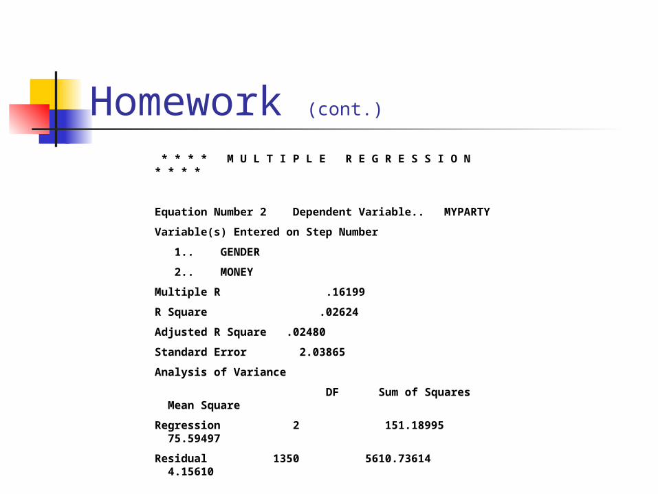
Equation Number 2 Dependent Variable.. MYPARTY
Variable(s) Entered on Step Number
1.. GENDER
2.. MONEY
Multiple R .16199
R Square .02624
Adjusted R Square .02480
Standard Error 2.03865
Analysis of Variance
DF Sum of Squares Mean Square
Regression 2 151.18995 75.59497
Residual 1350 5610.73614 4.15610
F = 18.18892 Signif F = .0000
Homework (cont.)
* * * * M U L T I P L E R E G R E S S I O N * * * *
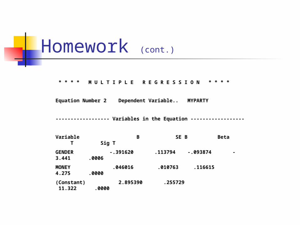
Equation Number 2 Dependent Variable.. MYPARTY
------------------ Variables in the Equation ------------------
Variable B SE B Beta T Sig T
GENDER -.391620 .113794 -.093874 -3.441 .0006
MONEY .046016 .010763 .116615 4.275 .0000
(Constant) 2.895390 .255729 11.322 .0000


![[David Epstein, Sharyn O'Halloran] Delegating Powe(BookZZ.org)](https://img.pdfslide.net/doc/110x75/563dbb59550346aa9aac625d/david-epstein-sharyn-ohalloran-delegating-powebookzzorg.jpg)