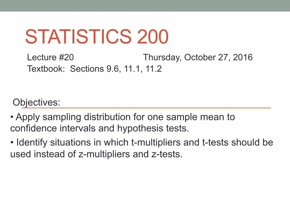
STATISTICS 200 Lecture #20 Thursday, October 27, 2016 Textbook: Sections 9.6, 11.1, 11.2

• Apply sampling distribution for one sample mean to confidence intervals and hypothesis tests. • Identify situations in which t-multipliers and t-tests should be used instead of z-multipliers and z-tests.

Objectives:

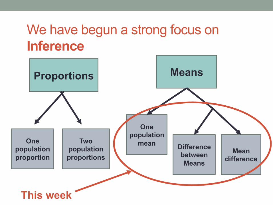
We have begun a strong focus on Inference

One population proportion

Two population proportions

One population

mean Difference between Means

Mean difference

Proportions Means

This week

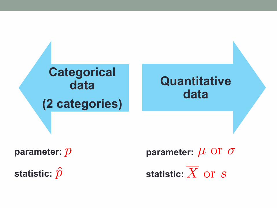
Categorical data

(2 categories)

Quantitative data

parameter: statistic:

parameter: statistic:

p

p̂

µ or �

X or s

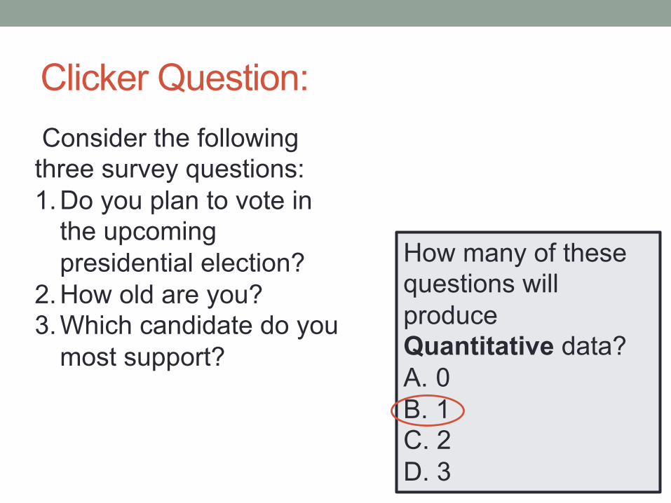
Clicker Question: Consider the following three survey questions: 1. Do you plan to vote in

the upcoming presidential election?

2. How old are you? 3. Which candidate do you

most support?

How many of these questions will produce Quantitative data? A.  0 B.  1 C.  2 D.  3

X sampling distribution52 68 84 100 116 132 148

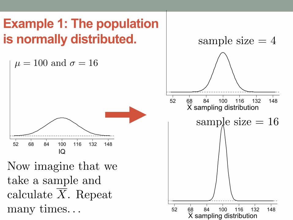
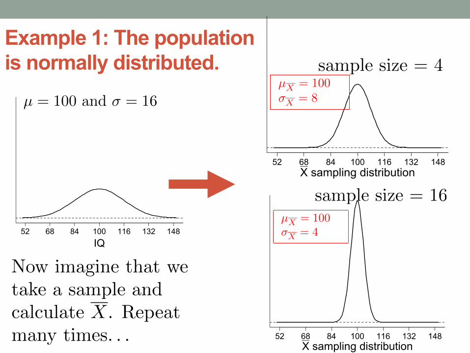
Example 1: The population is normally distributed.

X sampling distribution52 68 84 100 116 132 148

µ = 100 and � = 16

IQ52 68 84 100 116 132 148

sample size = 4

sample size = 16

Now imagine that we

take a sample and

calculate X. Repeat

many times. . .

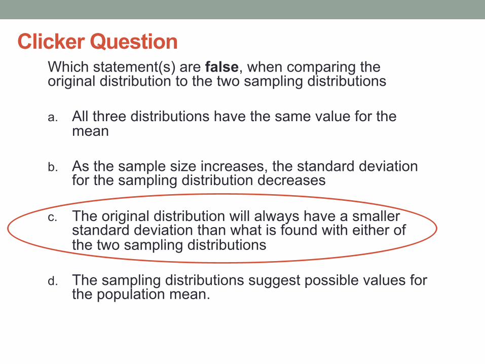
Clicker Question Which statement(s) are false, when comparing the

original distribution to the two sampling distributions a.  All three distributions have the same value for the

mean

b.  As the sample size increases, the standard deviation for the sampling distribution decreases

c.  The original distribution will always have a smaller standard deviation than what is found with either of the two sampling distributions

d.  The sampling distributions suggest possible values for the population mean.

X sampling distribution52 68 84 100 116 132 148

Example 1: The population is normally distributed.

X sampling distribution52 68 84 100 116 132 148

µ = 100 and � = 16

IQ52 68 84 100 116 132 148

sample size = 4

sample size = 16

Now imagine that we

take a sample and

calculate X. Repeat

many times. . .

µX = 100�X = 8

µX = 100�X = 4

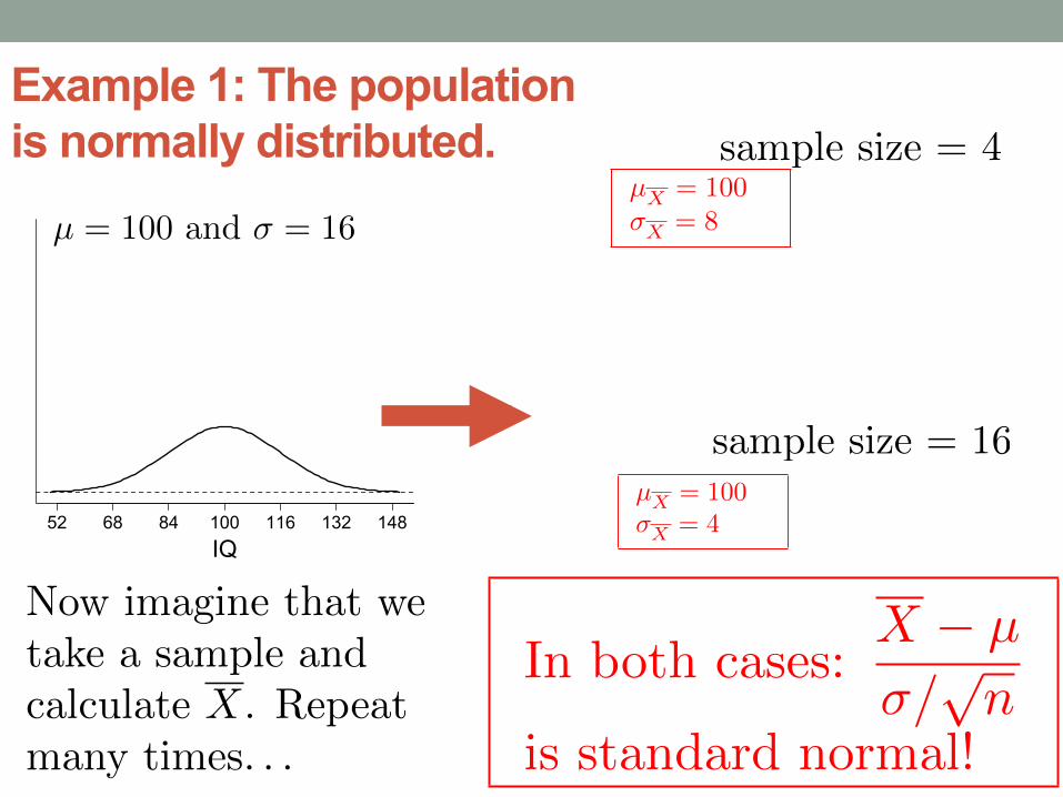
Example 1: The population is normally distributed.

µ = 100 and � = 16

IQ52 68 84 100 116 132 148

sample size = 4

sample size = 16

Now imagine that we

take a sample and

calculate X. Repeat

many times. . .

µX = 100�X = 8

µX = 100�X = 4

In both cases:

X � µ

�/pn

is standard normal!

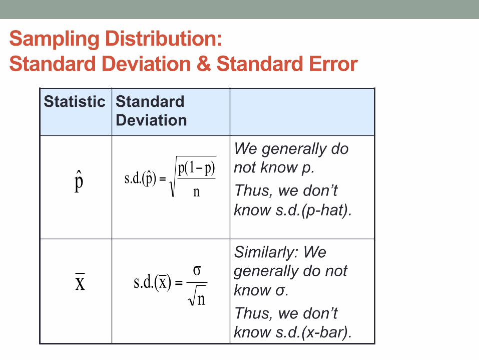
Sampling Distribution: Standard Deviation & Standard Error

Statistic Standard Deviation

We generally do not know p. Thus, we don’t know s.d.(p-hat).

Similarly: We generally do not know σ. Thus, we don’t know s.d.(x-bar).

np)p(1)p̂s.d.( −

=p̂

nσ)xs.d.( =x

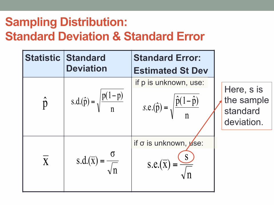
Sampling Distribution: Standard Deviation & Standard Error

Statistic Standard Deviation

Standard Error: Estimated St Dev

np)p(1)p̂s.d.( −

=p̂n)p̂(1p̂)p̂.e.( −

=s

ns)xs.e.( =n

σ)xs.d.( =x

if p is unknown, use:

if σ is unknown, use:

Here, s is the sample standard deviation.

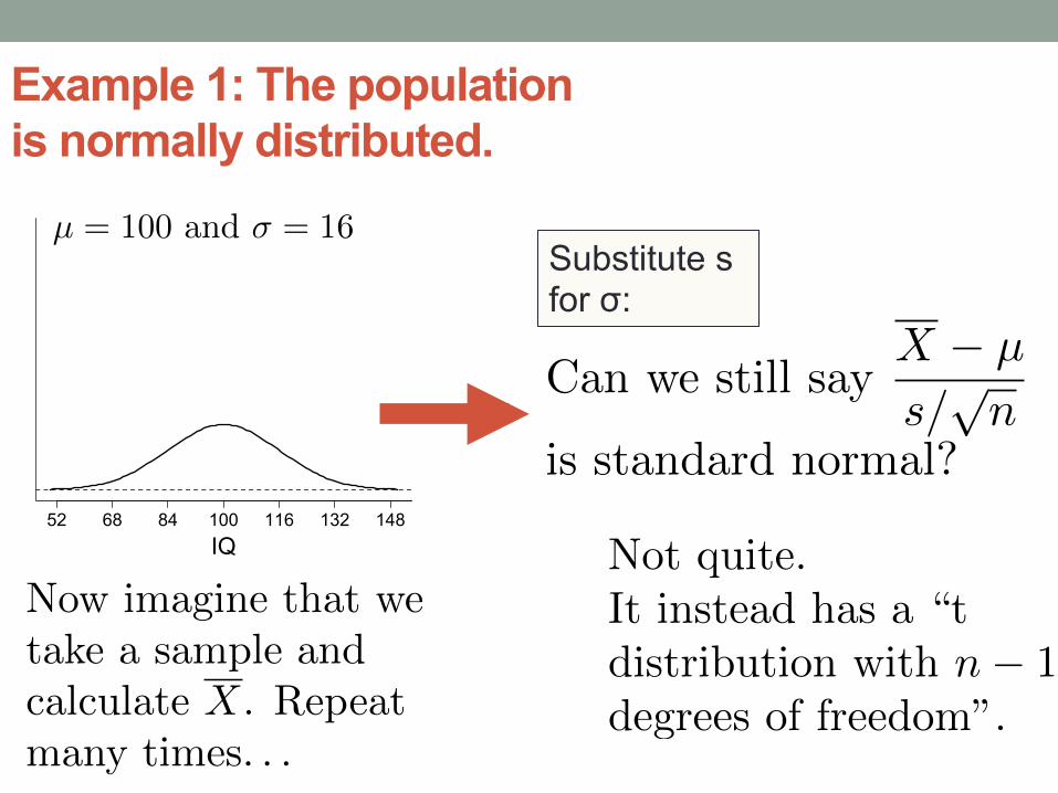
Example 1: The population is normally distributed.

µ = 100 and � = 16

IQ52 68 84 100 116 132 148

Now imagine that we

take a sample and

calculate X. Repeat

many times. . .

Can we still say

X � µ

s/pn

is standard normal?

Not quite.

It instead has a “t

distribution with n� 1

degrees of freedom”.

Substitute s for σ:

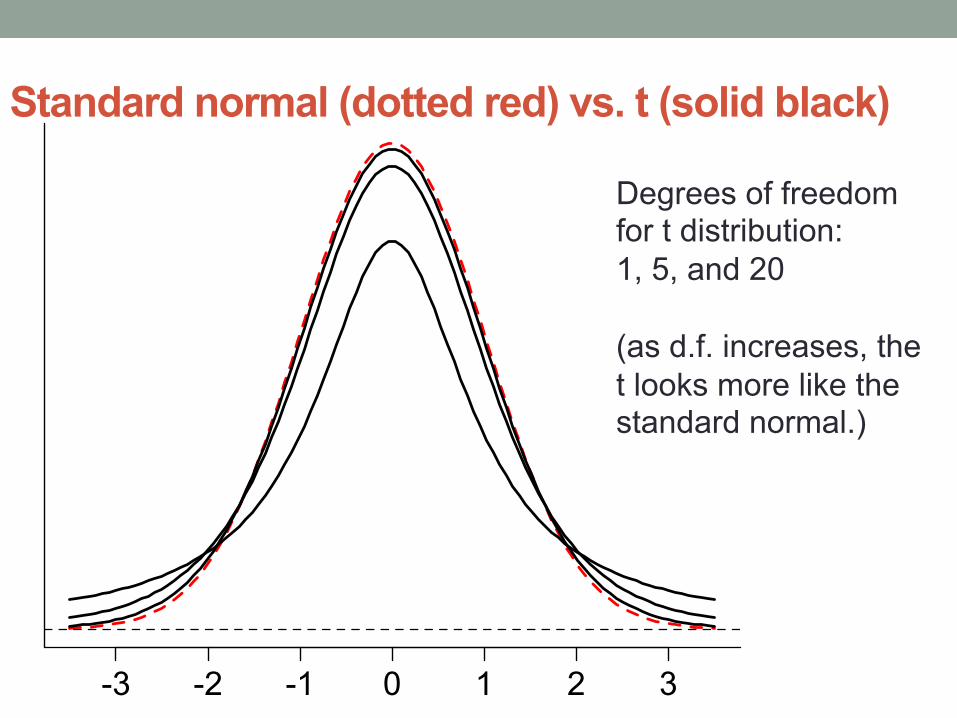
Standard normal (dotted red) vs. t (solid black)

-3 -2 -1 0 1 2 3

Degrees of freedom for t distribution: 1, 5, and 20 (as d.f. increases, the t looks more like the standard normal.)

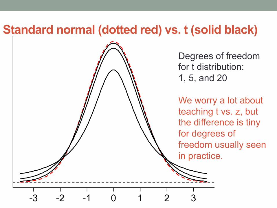
Standard normal (dotted red) vs. t (solid black)

-3 -2 -1 0 1 2 3

Degrees of freedom for t distribution: 1, 5, and 20 We worry a lot about teaching t vs. z, but the difference is tiny for degrees of freedom usually seen in practice.

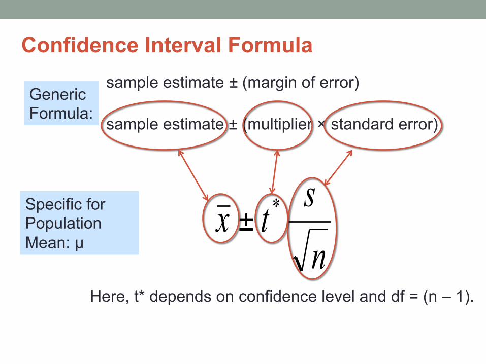
Confidence Interval Formula sample estimate ± (margin of error) sample estimate ± (multiplier × standard error)

nstx *±

Here, t* depends on confidence level and df = (n – 1).

Generic Formula:

Specific for Population Mean: µ

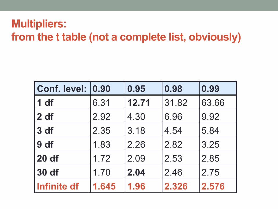
Multipliers: from the t table (not a complete list, obviously)

Conf. level: 0.90 0.95 0.98 0.99 1 df 6.31 12.71 31.82 63.66 2 df 2.92 4.30 6.96 9.92 3 df 2.35 3.18 4.54 5.84 9 df 1.83 2.26 2.82 3.25 20 df 1.72 2.09 2.53 2.85 30 df 1.70 2.04 2.46 2.75 Infinite df 1.645 1.96 2.326 2.576

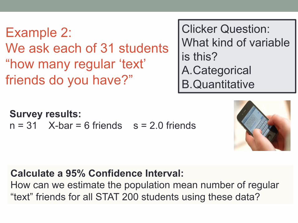
Example 2: We ask each of 31 students “how many regular ‘text’ friends do you have?”

Clicker Question: What kind of variable is this? A. Categorical B. Quantitative

Survey results: n = 31 X-bar = 6 friends s = 2.0 friends

Calculate a 95% Confidence Interval: How can we estimate the population mean number of regular “text” friends for all STAT 200 students using these data?

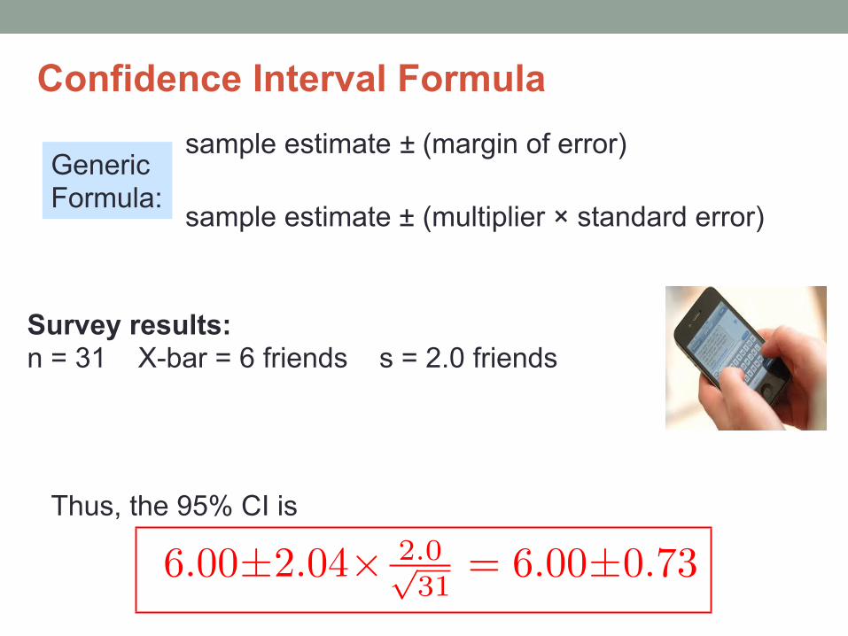
Confidence Interval Formula sample estimate ± (margin of error) sample estimate ± (multiplier × standard error)

Generic Formula:

Survey results: n = 31 X-bar = 6 friends s = 2.0 friends

6.00±2.04⇥ 2.0p31

= 6.00±0.73

Thus, the 95% CI is

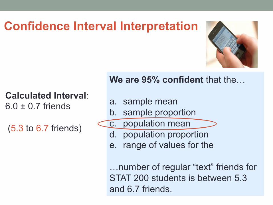
We are 95% confident that the… a.  sample mean b.  sample proportion c.  population mean d.  population proportion e.  range of values for the …number of regular “text” friends for STAT 200 students is between 5.3 and 6.7 friends.

Confidence Interval Interpretation

Calculated Interval: 6.0 ± 0.7 friends (5.3 to 6.7 friends)

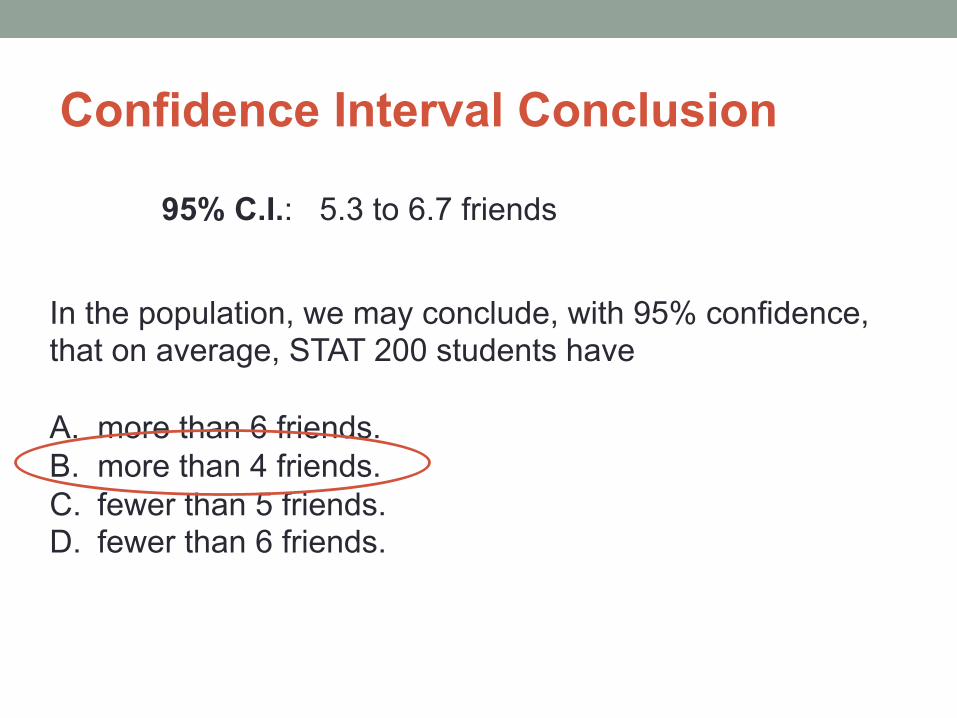
Confidence Interval Conclusion

In the population, we may conclude, with 95% confidence, that on average, STAT 200 students have A. more than 6 friends. B.  more than 4 friends. C.  fewer than 5 friends. D.  fewer than 6 friends.

95% C.I.: 5.3 to 6.7 friends

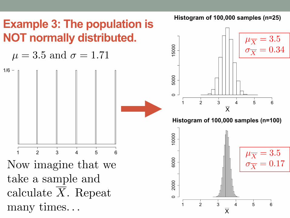
Histogram of 100,000 samples (n=25)

X1 2 3 4 5 6

05000

15000

Example 3: The population is NOT normally distributed.

Now imagine that we

take a sample and

calculate X. Repeat

many times. . .

µ = 3.5 and � = 1.71

1 2 3 4 5 6

1/6

µX = 3.5�X = 0.34

Histogram of 100,000 samples (n=100)

X1 2 3 4 5 6

02000

6000

10000

µX = 3.5�X = 0.17

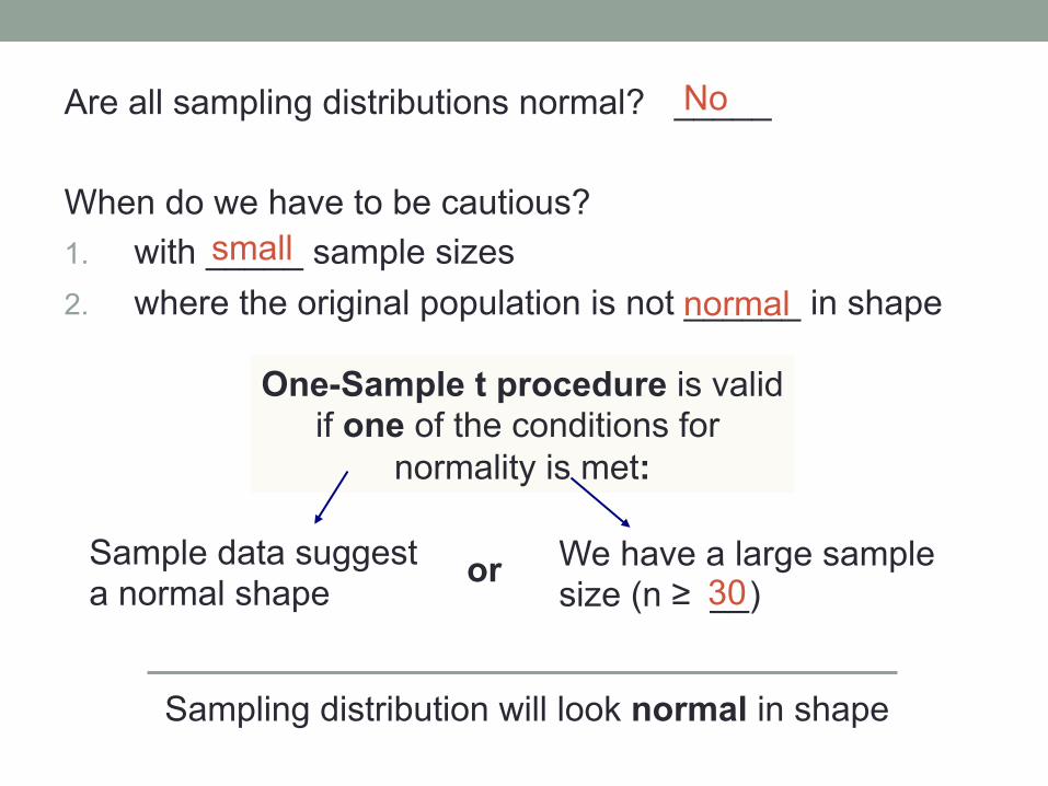
Are all sampling distributions normal? _____

When do we have to be cautious? 1.  with _____ sample sizes 2.  where the original population is not ______ in shape

One-Sample t procedure is valid if one of the conditions for

normality is met:

Sample data suggest a normal shape

We have a large sample size (n ≥ __)

or

Sampling distribution will look normal in shape

small

No

30

normal

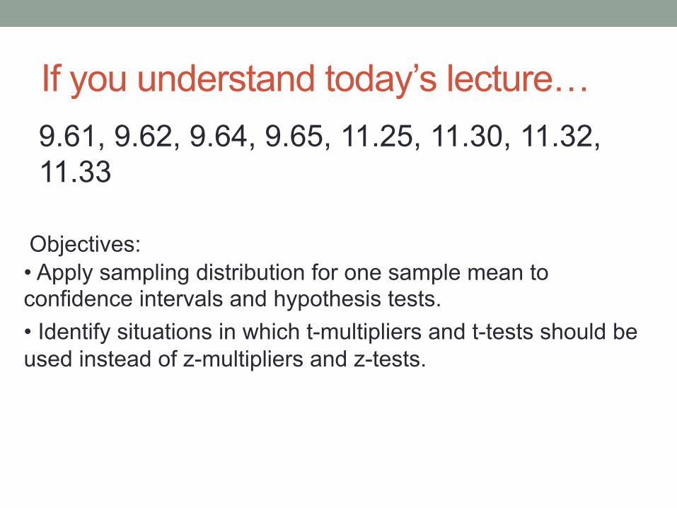
If you understand today’s lecture… 9.61, 9.62, 9.64, 9.65, 11.25, 11.30, 11.32, 11.33

Objectives: • Apply sampling distribution for one sample mean to confidence intervals and hypothesis tests. • Identify situations in which t-multipliers and t-tests should be used instead of z-multipliers and z-tests.