Statistics for BigData: Compressed Sensing, … Li Statistics for BigData: Compressed Sensing, Search, and Learning September, 2013 Simons Workshop 2 A Simple Interesting Story about

Ping Li Statistics for BigData: Compressed Sensing, Search, and Learning September, 2013 Simons Workshop 1

Statistics for BigData: Compressed Sensing, Search & Learn ing

Ping Li

Department of Statistics & Biostatistics

Department of Computer Science

Rutgers, the State University of New Jersey

Piscataway, NJ 08854

September 19, 2013


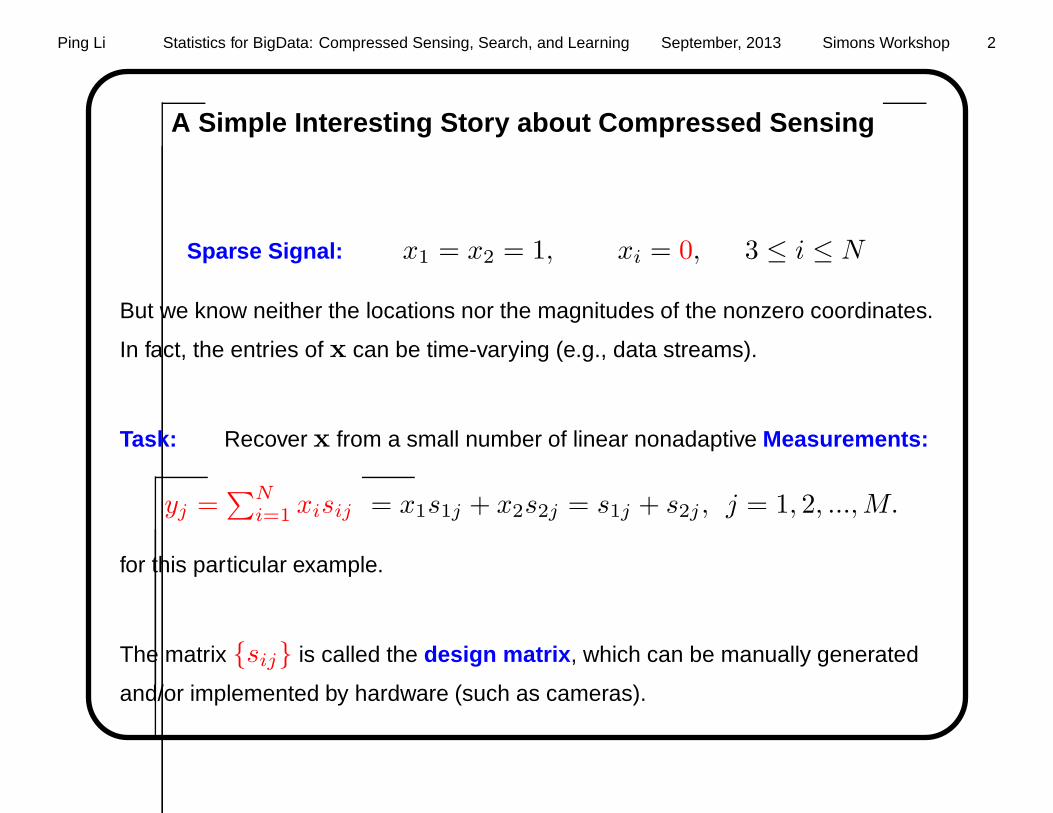
A Simple Interesting Story about Compressed Sensing

Sparse Signal: x1 = x2 = 1, xi = 0, 3 ≤ i ≤ N

But we know neither the locations nor the magnitudes of the nonzero coordinates.

In fact, the entries of x can be time-varying (e.g., data streams).

Task: Recover x from a small number of linear nonadaptive Measurements:

yj =∑N

i=1 xisij = x1s1j + x2s2j = s1j + s2j , j = 1, 2, ...,M.

for this particular example.

The matrix sij is called the design matrix , which can be manually generated

and/or implemented by hardware (such as cameras).


A 3-Iteration 3-Measurement Scheme

yj is the measurement vector and sij is the design matrix.

For this example, yj = s1j + s2j , j = 1, 2, ...,M .

Ratio Statistics:

z1,j = yj/s1j = 1 +s2js1j


zi,j = yj/sij =s1jsij

+s2jsij

, i ≥ 3

Ideal Design: s2j/s1j is either 0 or ±∞, i.e., z1,j = 1 or ±∞.


Suppose we use M = 3 measurements.

First coordinate z1,j = yj/s1j = 1 +s2js1j

Second coordinate z2,j = yj/s2j = 1 +s1js2j

Suppose s2j/s1j is either 0 or ±∞:

j = 1: Ifs2js1j

= 0, then z1,1 = 1 (truth), z2,1 = ±∞ (useless)

j = 2: Ifs2js1j

= ±∞, then z1,2 = ±∞ , z2,2 = 1

j = 3: Ifs2js1j

= 0, then z1,3 = 1, z2,3 = ±∞

With 3 measurements, we see z1,j = 1 twice and we safely estimate x1 = 1.


In the second iteration, we compute the residuals and update the ratio statistics:

rj = yj − x1s1j = s2j

z2,j = rj/s2j = 1, j = 1, 2, 3

Therefore, we can correctly estimate x2 = 1.


In the third iteration, we update the residual and ratio statistics:

rj = 0

zi,j = rj/sij = 0, i ≥ 3

This means, all zeros are identified.

An important (and perhaps surprising) consequence:

M = 3 measurements suffice for K = 2, regardless of N .

This in a sense contradicts the classical compressed sensing result that

O(K logN) measurements are needed.


Realization of the Ideal Design

It suffices to sample sij from α-stable distribution: sij ∼ S(α, 1) with α → 0.

The standard procedure : w ∼ exp(1), u ∼ unif(−π/2, π/2), w and u are

independent. Then

sin(αu)

(cosu)1/α

[cos(u− αu)

w

](1−α)/α

∼ S(α, 1)

which can be practically replaced by ± 1[unif(0,1)]1/α

.


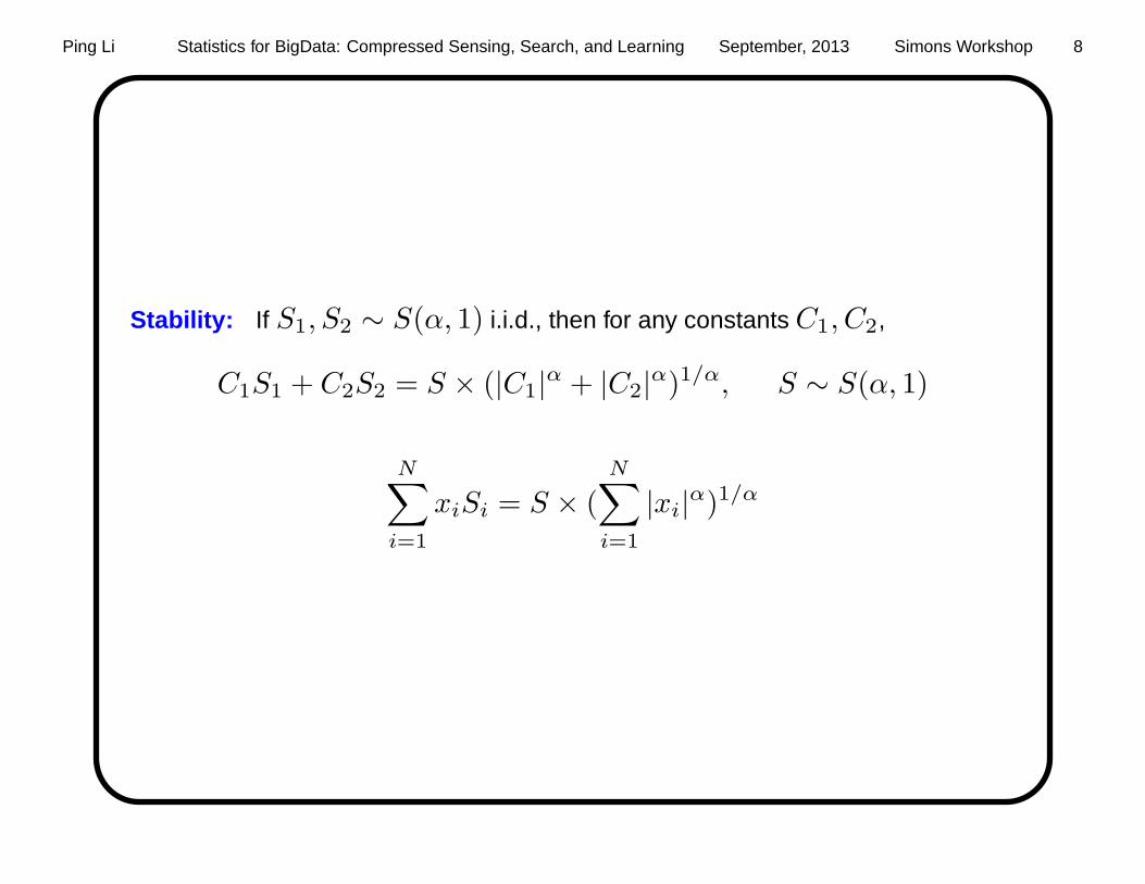
Stability: If S1, S2 ∼ S(α, 1) i.i.d., then for any constants C1, C2,

C1S1 + C2S2 = S × (|C1|α + |C2|α)1/α, S ∼ S(α, 1)

N∑

i=1

xiSi = S × (N∑

i=1

|xi|α)1/α


Ratio of Two Independent α-Stable Variables

S1, S2 ∼ S(α, 1) independent. Ratio |S2/S1| is either very small or very large.

0

0.1

0.2

0.3

0.4

0.5<10−6

10−6−0.010.01−100

100−106

>106

α = 0.03

Fre

quen

cy

0

0.1

0.2

0.3

0.4

0.5 <10−6

10−6−0.010.01−100

100−106

>106α = 0.02

Fre

quen

cy


0

0.1

0.2

0.3

0.4

0.5 <10−6

10−6−0.01

0.01−100

100−106

>106α = 0.01

Fre

quen

cy

0

0.1

0.2

0.3

0.4

0.5 <10−6

10−6−0.010.01−100

100−106

>106α = 0.001

Fre

quen

cy

Using very small α requires more precision. In this preliminary work, we simply

use Matlab and let α = 0.03.

————-

Recall, when K = 2, the ratio statistics are




Advantages of the New Compressed Sensing Framework

Our proposal uses α-stable distributions with 0 < α < 1, especially for small α.

• Computationally very efficient , with the main cost being one linear scan.

• Very robust to measurement noise , unlike traditional methods.

• Fewer (or at most the same) measurements compared to LP.

• The design matrix can be made very sparse easily especially for small α

(Related Ref: Ping Li, Very Sparse Stable Random Projections, KDD’07)

—————————-

A series of technical reports are being written, for example,

Ref: Ping Li, Cun-Hui Zhang, Tong Zhang, Compressed Counting Meets

Compressed Sensing, Preprint, 2013.


Compressed Counting Meets Compressed Sensing

Most natural signals (e.g., images) are nonnegative . Instead of using symmetric

stable projections, skewed stable projections have significant advantages.

——————-

Ref: Li Compressed Counting, SODA’09. (Initially written in 2007)

Ref: Li Improving Compressed Counting, UAI’09.

Ref: Li and Zhang A New Algorithm for Compressed Counting ..., COLT’11.

———————-

With Compressed Counting, a very simple recovery algorithm can be developed

and analyzed, at least for 0 < α ≤ 0.5


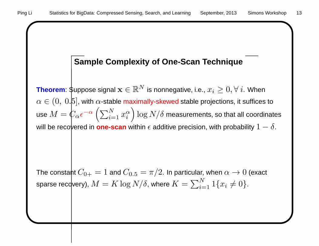
Sample Complexity of One-Scan Technique

Theorem : Suppose signal x ∈ RN is nonnegative, i.e., xi ≥ 0, ∀ i. When

α ∈ (0, 0.5], with α-stable maximally-skewed stable projections, it suffices to

use M = Cαǫ−α(

∑Ni=1 x

αi

)

logN/δ measurements, so that all coordinates

will be recovered in one-scan within ǫ additive precision, with probability 1− δ.

The constant C0+ = 1 and C0.5 = π/2. In particular, when α → 0 (exact

sparse recovery), M = K logN/δ, where K =∑N

i=1 1xi 6= 0.


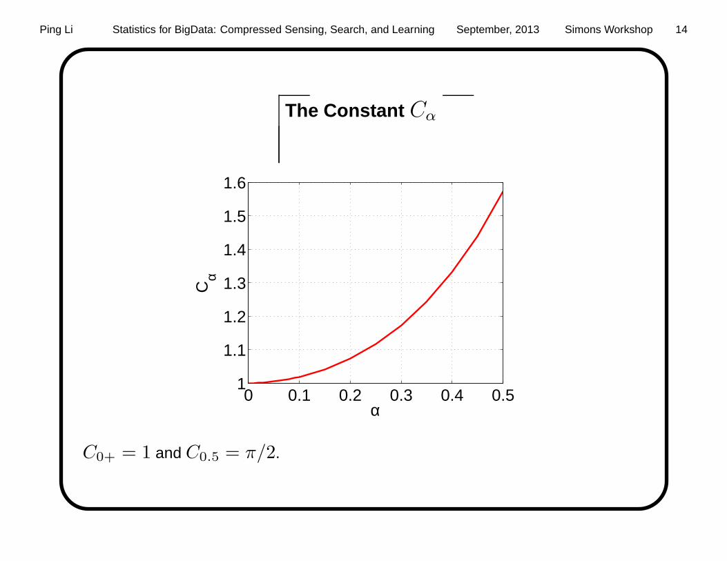
The Constant Cα

0 0.1 0.2 0.3 0.4 0.51

1.1

1.2

1.3

1.4

1.5

1.6

α

Cα

C0+ = 1 and C0.5 = π/2.


Extensions and Improvements

M = Cαǫ−α(

∑Ni=1 x

αi

)

logN/δ : Complexity for one-scan method using

Compressed Counting. Numerous extensions and improvements are possible:

• When the signal can be negative, use symmetric projections.

• If α → 0+, then ǫα → 1. This means we can accomplish exact sparse

recovery, which allows us to develop slightly more sophisticated multi-scan

(ie.., with iterations) algorithm. This will substantially reduce the required

number of measurements.

• Design matrix can be made extremely sparse with little impact on recovery.

(Related Ref: Ping Li, Very Sparse Stable Random Projections, KDD’07)


Simulations

Reconstruction error

Error =

√

√

√

√

∑Ni=1 (xi − estimated xi)

2

∑Ni=1 x

2i

, M0 = K logN/δ, M = M0/ζ

1 2 3 4 50

0.5

1

1.5

(1)

(2)(3)

OMP

LP

Med

ian

Err

or

ζ (# Measurements = M0/ζ)

Sign SignalN = 100000K = 100

1 2 3 4 50

0.5

1

1.5

(1)

(2)

(3)

OMP

LP

Med

ian

Err

or


Gaussian SignalN = 100000K = 100

Our proposed multi-scan algorithm with (1), (2), and (3) iterations, with small α.


Decoding Time

1 2 3 4 510

−1

100

101

102

103

(1)(2)

(3)

OMP

LP

Med

ian

Tim

e (s

ec)


Sign SignalN = 100000K = 100

1 2 3 4 510

−1

100

101

102

103

(1)(2)

(3)

OMP

LP

Med

ian

Tim

e (s

ec)


Gaussian SignalN = 100000K = 100


An Example of “Single-Pixel Camera” Application

The task is to take a picture using linear combination of measurements. When the

scene is sparse, our method can efficiently recover the nonzero components.

Original

In reality, natural pictures are often not as sparse, but in important scenarios, for

example, the difference between consecutive frames of surveillance cameras are

usually very sparse because the background remains still.


M = K log(N/δ)/ζ measurements.

Original ζ = 1, Time = 11.63

ζ = 3, Time = 4.61 ζ = 15, Time = 4.94


Summary of Contributions on Compressed Sensing

• Sparse recovery is a very active area of research in many disciplines:

Mathematics, EE, CS, and perhaps Statistics.

• In classical settings, the design matrix for sparse recovery is sampled from

Gaussian distribution, which is α = 2-stable distribution.

• Using α-stable distribution with α ≈ 0 leads to simple, fast, robust, accurate

exact sparse recovery. Cost is one linear scan, with no catastrophic failures.

• The design matrix can be made very sparse without hurting the performance.

This connects to the influential work on sparse recovery with sparse matrices.

• This is just very preliminary work. There are numerous research problems

and applications which we will study in the next a few years.


Other Applications of Stable Random Projections

yj =∑N

i=1 xisij , sij ∼ S(α, β, 1), i.e., α-stable, β-skewed.

• Estimating the lα norm (∑N

i=1 |xi|α) or distance in streaming data.

Ref: Indyk JACM’06, Li SODA’08.

• Using skewed projections with β = 1 (Compressed Counting) makes entropy

estimation trivial in nonnegative data streams (10 samples are needed).

Ref: Li SODA’09, Li UAI’09, Li and Zhang COLT’11

• Using dependent symmetric (β = 0) projections also makes entropy

estimation trivial in general data streams (100 samples are needed).

Ref: Li and Zhang, Correlated Symmetric Stable Random Projections,

NIPS’12.


yj =∑N

i=1 xisij

• Using only the signs (sign(yj), i.e., 1-bit) of the projected data leads to very

efficient search and machine learning algorithms. For example, sign Cauchy

(i.e., α = 1) projection implicitly (and approximately) compute the χ2-kernel

(which is very popular in Computer Vision) with a linear kernel.

Ref: Li, Samorodnitsky, and Hopcroft, Sign Cauchy Projections and

Chi-Square Kernel, NIPS’13.

• We can make better use of more than just the signs (i.e., more than 1-bit) of

the projected data.

Ref: Li, Mitzenmacher, and Shrivastava, Coding for Random Projections,

arXiv’1308.2218.


Data Streams and Entropy Estimation

• Massive data generated as streams and processed on the fly in one-pass .

The problem of “scaling up for high dimensional data and high speed data

streams” is among the “ten challenging problems in data mining research”.

• In the standard turnstile model , a data stream is a vector At of length N ,

where N = 264 or N = 2128 in network applications. At time t, there is an

input stream at = (it, It), it ∈ [1, N ] which updates At by a linear rule:

At[it] = At−1[it] + It.

• A crucial task is to compute the α-th moment F(α) and Shannon entropy H :

F(α) =N∑

i=1

|At[i]|α, H = −N∑

i=1

|At[i]|F1

log|At[i]|F1

,

Exact computation is not feasible as it requires storing the entire vector At.


Anomaly Detection of Network Traffic

Network traffic is a typical example of high-rate data streams. An effective

measurement in real-time is crucial for anomaly detection and network diagnosis.

200 400 600 800 1000 12000123456789

10

packet counts (thousands)

source IP address: entropy value

This plot is reproduced from a DARPA conference (Feinstein et. al. 2003). One

can view x-axis as surrogate for time. Y-axis is the measured Shannon entropy,

which exhibited a sudden sharp change at the time when an attack occurred.


Entropy Estimation Using Derivatives

The Shannon entropy is essentially the derivative of the frequency moment at

α = 1. A popular practice is to approximate Shannon entropy by finite difference:

Hα =1

α− 1

(

1− F(α)

Fα(1)

)

−→ H, as α → 1

and then estimate H by estimating the two moments Fα(1) and F(α)

Hα =1

α− 1

(

1− F(α)

Fα(1)

)

The immediate problem is that

V ar(

Hα

)

= O

(

1

|α− 1|2)

but α → 1

Before our work, entropy estimation needs lots of samples, millions or billions.


Compressed Counting for Nonnegative Data Streams

For nonnegative data streams (as common in practice), the first moment can be

computed error-free: (Recall At[it] = At−1[it] + It)

F(1) =

N∑

i=1

|At[i]| =N∑

i=1

At[i] =

t∑

s=1

Is

Thus, we should expect V ar(

F(1)

)

= 0. It turns out using maximally-skewed

stable random projections, we can achieve extremely small variance:

V ar(

F(α)

)

= Θ(

|α− 1|2)

This essentially makes entropy estimation a trivial problem because now

V ar(

H(α)

)

= const instead of O(

1|α−1|2

)

.


The Estimator For Nonnegative Data Streams

xj =N∑

i=1

At[i]sij , sij ∼ S(α, β = 1, 1)

F(α) =1

∆∆

[

k∑k

j=1 x−α/∆j

]∆

, ∆ = 1− α

V ar(

F(α)

)

= Θ(

|α− 1|2)


10 Samples Provide Good Estimates

10−8

10−6

10−4

10−2

100

10−5

10−4

10−3

10−2

10−1

100

101

∆ = 1−α

Nor

mal

ized

MS

E

A: H, new

k=1000

k=100

k=10

k=3

Ref: Li Compressed Counting, SODA’09. (Initially written in 2007)

Ref: Li Improving Compressed Counting, UAI’09.

Ref: Li and Zhang A New Algorithm for Compressed Counting ..., COLT’11.


Dependent Symmetric Stable Projections for General Stream s

For general streams (e.g., difference between two streams), we have to use

symmetric stable projections.

Hα =1

α− 1

(

1− F(α)

Fα(1)

)

−→ H, as α → 1

The idea is to make the two estimators, F(1) and F(α), highly dependent to

reduce the variance.

This technique also makes V ar(

H(α)

)

= const, by using a special sampling

procedure and (seemingly) strange estimator.


Recall, If w ∼ exp(1), u ∼ unif(−π/2, π/2), w and u are independent,

then

g(u,w;α) =sin(αu)

(cosu)1/α

[cos(u− αu)

w

](1−α)/α

∼ S(α, 1)

and g(u,w;α) ∼ S(1, 1).

Thus, we can use g(u,w; 1) to estimate F(1), and g(u,w;α) to estimate F(α).

The two estimators ought to be highly dependent.

Surprisingly, in order to remove the O(

1|α−1|2

)

factor in Hα, we must use a

special and bad estimator for F(α). Magically, the ratio of the two “bad”

estimatorsF(α)

Fα(1)

leads to a good estimate of H .


The Estimator of Entropy in General Data Streams

wij ∼ exp(1), uij ∼ uniform(−π/2, π/2)

xj =N∑

i=1

At[i]g(wij , uij , 1), yj =N∑

i=1

At[i]g(wij , uij , α)

Hα =1

α− 1

1−( √

π

Γ(

1− 12α

)

∑kj=1

√

|yj |∑k

j=1

√

|xj |

)2α


100 Samples Provide Good Estimate in General Streams

10−5

10−4

10−3

10−2

10−1

100

10−4

10−3

10−2

10−1

100

k = 10

k = 100

k = 1000

A−THE : Corr. γ = 0.5

∆ = α − 1

Nor

mal

ized

MS

E

Ref: Li and Zhang Entropy Estimations Using Correlated Symmetric Stable

Random Projections, NIPS’12.


Limitations of Stable Random Projections

When the high-dimensional data are binary and extremely sparse (as common in

practice), it is often much more efficient to use b-bit minwise hashing .

This is illustrated by our work on machine learning with bigdata .


Practice of Statistical Analysis and Data Mining

Key Components :

Models (Methods) + Variables (Features) + Observations (Examples)

A Popular Practice :

Simple Models + Lots of Features + Lots of Data

or simply

Simple Methods + BigData


BigData Everywhere

Conceptually, consider a dataset as a matrix of size n×D.

In modern applications, # examples n = 106 is common and n = 109 is not

rare, for example, images, documents, spams, search click data.

High-dimensional (image, text, biological) data are common: D = 106 (million),

D = 109 (billion), D = 1012 (trillion), or even D = 264.


Examples of BigData Challenges: Linear Learning

Binary classification: Dataset (xi, yi)ni=1, xi ∈ RD , yi ∈ −1, 1.

One can fit an L2-regularized linear logistic regression:

minw

1

2w

Tw +C

n∑

i=1

log(

1 + e−yiwTxi

)

,

or the L2-regularized linear SVM:

minw

1

2w

Tw +C

n∑

i=1

max

1− yiwTxi, 0

,

where C > 0 is the penalty (regularization) parameter.


Challenges of Learning with Massive High-dimensional Data

• The data often can not fit in memory (even when the data are sparse).

• Data loading (or transmission over network) takes too long.

• Training can be expensive, even for simple linear models.

• Testing may be too slow to meet the demand, especially crucial for

applications in search, high-speed trading, or interactive data visual analytics.

• Near neighbor search, for example, finding the most similar document in

billions of Web pages without scanning them all.


Dimensionality Reduction and Data Reduction

Dimensionality reduction: Reducing D, for example, from 264 to 105.

Data reduction: Reducing # nonzeros is often more important. With modern

linear learning algorithms, the cost (for storage, transmission, computation) is

mainly determined by # nonzeros, not much by the dimensionality.

———————

In practice, where do high-dimensional data come from?


Webspam: Text Data

Dim. Time Accuracy

1-gram 254 20 sec 93.30%

3-gram 16,609,143 200 sec 99.6%

Kernel 16,609,143 About a Week 99.6%

Classification experiments were based on linear SVM unless marked as “kernel”

—————-

(Character) 1-gram : Frequencies of occurrences of single characters.

(Character) 3-gram : Frequencies of occurrences of 3-contiguous characters.


Webspam: Binary Quantized Data

Dim. Time Accuracy

1-gram 254 20 sec 93.30%

Binary 1-gram 254 20 sec 87.78%

3-gram 16,609,143 200 sec 99.6%

Binary 3-gram 16,609,143 200 sec 99.6%

Kernel 16,609,143 About a Week 99.6%

With high-dim representations, often only presence/absence information matters.


Major Issues with High-Dim Representations

• High-dimensionality

• High storage cost

• Relatively high training/testing cost

The search industry has commonly adopted the practice of

high-dimensional data + linear algorithms + hashing

——————

Random projection is a standard hashing method.

Several well-known hashing algorithms are equivalent to random projections.


A Popular Solution Based on Normal Random Projections

Random Projections : Replace original data matrix A by B = A×R

A R = B

R ∈ RD×k: a random matrix, with i.i.d. entries sampled from N(0, 1).

B ∈ Rn×k : projected matrix, also random.

B approximately preserves the Euclidean distance and inner products between

any two rows of A. In particular, E (BBT) = AE(RR

T)AT = AAT.

Therefore, we can simply feed B into (e.g.,) SVM or logistic regression solvers.


Very Sparse Random Projections

The projection matrix: R = rij ∈ RD×k. Instead of sampling from normals,

we sample from a sparse distribution parameterized by s ≥ 1:

rij =

−1 with prob. 12s

0 with prob. 1− 1s

1 with prob. 12s

If s = 100, then on average, 99% of the entries are zero.

If s = 1000, then on average, 99.9% of the entries are zero.

——————-

Ref: Li, Hastie, Church, Very Sparse Random Projections, KDD’06.

Ref: Li, Very Sparse Stable Random Projections, KDD’07.


A Running Example Using (Small) Webspam Data

Datset: 350K text samples, 16 million dimensions, about 4000 nonzeros on

average, 24GB disk space.

0 2000 4000 6000 8000 100000

1

2

3

4x 10

4

# nonzeros

Fre

quen

cy

Webspam

Task: Binary classification for spam vs. non-spam.

——————–

Data were generated using character 3-grams, i.e., every 3-contiguous

characters.


Very Sparse Projections + Linear SVM on Webspam Data

Red dashed curves: results based on the original data

10−2

10−1

100

101

102

75

80

85

90

95

100

k = 32

k = 64

k = 128

k = 256k = 512k = 1024k = 4096

Webspam: SVM (s = 1)

C

Cla

ssifi

catio

n A

cc (

%)

10−2

10−1

100

101

102

75

80

85

90

95

100

k = 32

k = 64

k = 128

k = 256k = 512k = 1024k = 4096

Webspam: SVM (s = 1000)

CC

lass

ifica

tion

Acc

(%

)Observations:

• We need a large number of projections (e.g.,k > 4096) for high accuracy.

• The sparsity parameter s matters little, i.e., matrix can be very sparse.


Disadvantages of Random Projections (and Variants)

Inaccurate, especially on binary data.

Ref: Li, Hastie, and Church, Very Sparse Random Projections, KDD’06.

Ref: Li, Shrivastava, Moore, Konig, Hashing Algorithms for Large-Scale Learning, NIPS’11


The New Approach

• Use random permutations instead of random projections.

• Use only a small “k” (e.g.,) 200 as opposed to (e.g.,) 104.

• The work is inspired by minwise hashing for binary data.

—————

This talk will focus on binary data.


Minwise Hashing

• In information retrieval and databases, efficiently computing similarities is

often crucial and challenging, for example, duplicate detection of web pages.

• The method of minwise hashing is still the standard algorithm for estimating

set similarity in industry, since the 1997 seminal work by Broder et. al.

• Minwise hashing has been used for numerous applications, for example:

content matching for online advertising, detection of large-scale redundancy

in enterprise file systems, syntactic similarity algorithms for enterprise

information management, compressing social networks, advertising

diversification, community extraction and classification in the Web graph,

graph sampling, wireless sensor networks, Web spam, Web graph

compression, text reuse in the Web, and many more.


Binary Data Vectors and Sets

A binary (0/1) vector in D-dim can be viewed a set S ⊆ Ω = 0, 1, ..., D − 1.

Example: S1, S2, S3 ⊆ Ω = 0, 1, ..., 15 (i.e., D = 16).

0 1 2 3 4 5 6 7 8 9 10 11 12 13 14 15

0

0

0

1

0

0

0

0

0

0

0

1

1

0

0

1

0

0

0

0

1

0

0

1

1

1

0

0

0

0

0

1

0

0

0

0

1

0

0

0

0

0

1

1

0

0

0

S1:

S2:

S3:

0

S1 = 1, 4, 5, 8, S2 = 8, 10, 12, 14, S3 = 3, 6, 7, 14


Minwise Hashing in 0/1 Data Matrix

Original Data Matrix

0 1 2 3 4 5 6 7 8 9 10 11 12 13 14 15

0

0

0

1

0

0

0

0

0

0

0

1

1

0

0

1

0

0

0

0

1

0

0

1

1

1

0

0

0

0

0

1

0

0

0

0

1

0

0

0

0

0

1

1

0

0

0

S1:

S2:

S3:

0

Permuted Data Matrix

0 1 2 3 4 5 6 7 8 9 10 11 12 13 14 15

0

1

1

0

0

1

1

0

0

0

1

0

1

0

0

0

0

0

0

1

0

1

0

0

0

0

0

0

0

0

0

0

1

0

0

0

0

0

1

1

1

0

0

0

0

0

0

0

π(S1):

π(S2):

π(S3):

min(π(S1)) = 2, min(π(S2)) = 0, min(π(S3)) = 0


An Example with k = 3 Permutations

Input: sets S1, S2, ...,

Hashed values for S1 : 113 264 1091

Hashed values for S2 : 2049 103 1091

Hashed values for S3 : ...

....

—————————-

One major problem : Need to use 64 bits to store each hashed value.


Issues with Minwise Hashing and Our Solutions

1. Expensive storage (and computation) : In the standard practice, each

hashed value was stored using 64 bits.

Our solution: b-bit minwise hashing by using only the lowest b bits.

2. Linear kernel learning : Minwise hashing was not used for supervised

learning, especially linear kernel learning.

Our solution: We prove that (b-bit) minwise hashing results in positive definite

(PD) linear kernel matrix. The data dimensionality is reduced from 264 to 2b.

3. Expensive and energy-consuming (pre)processing for k permutations :

The industry had been using the expensive procedure since 1997 (or earlier)

Our solution: One permutation hashing, which is even more accurate.


All these are accomplished by only doing basic statistics/p robability


Ref: Li and Konig, b-Bit Minwise Hashing, WWW’10.

Ref: Li and Konig, Theory and Applications of b-Bit Minwise Hashing, CACM

Research Highlights, 2011 .

Ref: Li, Konig, Gui, b-Bit Minwise Hashing for Estimating 3-Way Similarities,

NIPS’10.

Ref: Shrivastava and Li, Fast Near Neighbor Search in High-Dimensional Binary

Data, ECML’12

Ref: Li, Owen, Zhang, One Permutation Hashing, NIPS’12


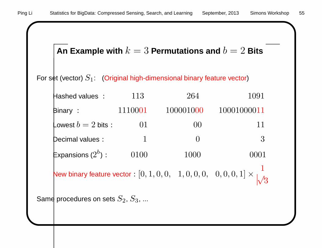
An Example with k = 3 Permutations and b = 2 Bits

For set (vector) S1: (Original high-dimensional binary feature vector)

Hashed values : 113 264 1091

Binary : 1110001 100001000 10001000011

Lowest b = 2 bits : 01 00 11

Decimal values : 1 0 3

Expansions (2b) : 0100 1000 0001

New binary feature vector : [0, 1, 0, 0, 1, 0, 0, 0, 0, 0, 0, 1]× 1√3

Same procedures on sets S2, S3, ...


Experiments on Webspam Data: Testing Accuracy

10−3

10−2

10−1

100

101

102

80828486889092949698

100

C

Acc

urac

y (%

)

b = 6,8,10,16

b = 1

svm: k = 200

b = 24

b = 4

Spam: Accuracy

• Dashed: using the original data (24GB disk space).

• Solid: b-bit hashing. Using b = 8 and k = 200 achieves about the same test

accuracies as using the original data. Space: 70MB (350000× 200)


Training Time

10−3

10−2

10−1

100

101

102

100

101

102

103

C

Tra

inin

g tim

e (s

ec)

b = 16

svm: k = 200Spam: Training time

• They did not include data loading time (which is small for b-bit hashing)

• The original training time is about 200 seconds.

• b-bit minwise hashing needs about 3 ∼ 7 seconds (3 seconds when b = 8).


Testing Time

10−3

10−2

10−1

100

101

102

12

10

100

1000

C

Tes

ting

time

(sec

)svm: k = 200Spam: Testing time

However, here we assume the test data have already been processed.


The Problem of Expensive Preprocessing

200 or 500 permutations on the entire data can be very expensive.

Particularly a serious issue when the new testing data have not been processed.

Two solutions:

1. Parallel solution by GPUs : Achieved up to 100-fold improvement in speed.

Ref: Li, Shrivastava, Konig, GPU-Based Minwise Hashing, WWW’12 (poster)

2. Statistical solution : Only one permutation is needed. Even more accurate.

Ref: Li, Owen, Zhang, One Permutation Hashing, NIPS’12


Intuition: Minwise Hashing Ought to Be Wasteful

Original Data Matrix

0 1 2 3 4 5 6 7 8 9 10 11 12 13 14 15

0

0

0

1

0

0

0

0

0

0

0

1

1

0

0

1

0

0

0

0

1

0

0

1

1

1

0

0

0

0

0

1

0

0

0

0

1

0

0

0

0

0

1

1

0

0

0

S1:

S2:

S3:

0

Permuted Data Matrix

0 1 2 3 4 5 6 7 8 9 10 11 12 13 14 15

0

1

1

0

0

1

1

0

0

0

1

0

1

0

0

0

0

0

0

1

0

1

0

0

0

0

0

0

0

0

0

0

1

0

0

0

0

0

1

1

1

0

0

0

0

0

0

0

π(S1):

π(S2):

π(S3):

Only store the minimums and repeat the process k (e.g., 500) times.


One Permutation Hashing

S1, S2, S3 ⊆ Ω = 0, 1, ..., 15 (i.e., D = 16). After one permutation:

π(S1) = 2, 4, 7, 13, π(S2) = 0, 3, 6, 13, π(S3) = 0, 1, 10, 12

0 1 2 3 4 5 6 7 8 9 10 11 12 13 14 15

0

1

1

0

0

1

1

0

0

0

1

0

1

0

0

0

0

0

0

1

0

1

0

0

0

0

0

0

0

0

0

0

1

0

0

0

0

0

1

1

1

0

0

0

0

0

0

0

1 2 3 4

π(S1):

π(S2):

π(S3):

One permutation hashing: divide the space Ω evenly into k = 4 bins and

select the smallest nonzero in each bin.

Ref: P. Li, A. Owen, C-H Zhang, One Permutation Hashing, NIPS’12


Experimental Results on Webspam Data

10−3

10−2

10−1

100

101

102

80828486889092949698

100

C

Acc

urac

y (%

)

b = 1b = 2

b = 4b = 6,8

SVM: k = 256Webspam: Accuracy

Original1 Permk Perm

10−3

10−2

10−1

100

101

102

80828486889092949698

100

CA

ccur

acy

(%)

b = 1

b = 2b = 4,6,8

SVM: k = 512Webspam: Accuracy

Original1 Permk Perm

One permutation hashing (zero coding) is even slightly more accurate than

k-permutation hashing (at merely 1/k of the original cost).


Summary of Contributions on b-Bit Minwise Hashing

1. b-bit minwise hashing : Use only the lowest b bits of hashed value, as

opposed to 64 bits in the standard industry practice.

2. Linear kernel learning : b-bit minwise hashing results in positive definite

linear kernel. The data dimensionality is reduced from 264 to 2b.

3. One permutation hashing : It reduces the expensive and energy-consuming

process of (e.g.,) 500 permutations to merely one permutation. The results

are even more accurate.

4. Beyond Pairwise: three-way hashing and search (e.g., Googl eSets) :

Ref: Li, Konig, Gui, NIPS’10. Ref: Shrivastava and Li, NIPS’13.

5. Others: For example, b-bit minwise hashing naturally leads to a

space-partition scheme for sub-linear time near-neighbor search.


Conclusion

• The “Big Data” time . Researchers & practitioners often don’t have enough

knowledge of the fundamental data generation process, which is fortunately

often compensated by the capability of quickly collecting lots of data.

• Approximate answers often suffice , for many statistical problems.

• Hashing becomes crucial in important applications , for example, search

engines, as they have lots of data and need the answers quickly & cheaply.

• Hashing with stable random projections leads to surprising algorithms for

compressed sensing (sparse signal recovery), databases, learning, and

information retrieval. Numerous research problems remain to be solved.

• Binary data are special and crucial . In most applications, one can expand

the features to extremely high-dimensional binary vectors.


• b-Bit minwise hashing , in important applications, often provides significantly

better results than stable random projections.

• Probabilistic hashing is basically clever sampling .

• Numerous interesting research problems . Statisticians can make great

contributions in this area. We just need to treat them as statistical problems.

Documents

Statistics for BigData: Compressed Sensing, … Li Statistics for BigData: Compressed Sensing, Search, and Learning September, 2013 Simons Workshop 2 A Simple Interesting Story about