Statistics in Archaeology: New directions

Pedro Delicado Departament d'Economia i Empresa, Universität Pompeu Fabra

Ramon Trias Fargas 25-27, 08005 Barcelona, Spain. E-mail; delicado@upf.es

Abstract

Connections between Statistics and Archaeology have always appeared very fruitful The objective of this paper is to offer an outlook of some statistical techniques that are being developed in the most recent years and that can be of interest for archaeologists in the short run.

Key Words: Artificial Neural Networks. Bayesian Statistics. Bootstrap. Multivariate Analysis. Nonparametric Statistics. Statistical Software.

1 Introduction

Scientific research is not outside the world-wide extension process that many aspects of the live are experimenting at the end of the century. Connections between different areas are easier and easier. On the other hand, specialization is almost a requirement to be able to contribute significantly in any field of the scientific spectrum. So it is frequent to fmd researchers coming from very different areas who work on the same kind of problems.

This atmosphere favors that links between Statistics and Archaeology become even stronger than they traditionally were. This paper attempts to throw some light on the topics that statisticians are dealing with, in the hope that archaeologists are incorporating them to their usual research activities.

There are many stages in an archaeological research process where statistical problems are present. The problem of data collection appears first. Sampling techniques and experimental design offer good classical solutions and no new contributions are being referred here. We just turn to remark once agam that an appropriate random selection of the data is crucial to validate posterior inference procedures.

Once data have been collected, the archeologist is concerned about see her data. Exploratory Data Analysis is then to her service. Here we refer to that matter when we explain some nonparametric methods (subsection 2.1) and multivariate methods (section 4).

Statistical inference is broadly present in Archaeology. Dating methods, typology (cluster analysis) and discriminant analysis are maybe the most popular of these procedures. Recent advances are compiled in sections 2, 3, and 6. Bootstrap and other resampling methods are the content of section 5. They turn out to be useful general tools for validating and calibrating inference methods.

A common problem in many practical studies is the simultaneous presence of qualitative and quantitative information. Some of the techniques developed here are specially adequate to deal with this problem. It is proper to emphasize multivariate methods based on distances (subsection 4.3) and Bayesian methods (section 6).

Section 7 quickly reviews some statistical packages. It also includes a list of Intemet resources where statistical software related with Archaeology is accessible.

We are not reviewing the field known as Spatial Statistics notwithstanding that it is an important connection area between Statistics and Archaeology. Only some recent references are listed: is dedicated to Spatial Statistics, and has a chapter about the Bayesian analysis of spatial data.

The rest of the paper is organized by statistical topics. It is hoped that at the end of the paper the correspondence between reviewed statistical methods and archaeological problems looks clear.

2 Nonparametric methods

We call nonparametric methods to the statistical techniques dealing with the estimation of flinctionals of the density or regression function. There are no parametric assiunptions involved in the estimation (for instance, no normality assumptions are made) or we can think that the parameter space has infmite dimension (for instance, each possible density function could be a parameter; then the parameter space would be the set of all possible functions, who has infmite dimension). Strictly speaking, nonparametric methods are not a novelty neither in Statistics nor in Archaeology (a simple histogram is a nonparametric estimator of a density function), but in our opinion all their potential has not been fully explored. We present here density estimation by kernel methods, and regression fiinction estimation performed by three different approaches.

2.1 Kernel density and regression estimation

The objective is to estimate the density function (i.e. the \di\\xtf(x) of the density function of a random variable .Y at a point X, given a random sample of X: X,,.....^„) or the regression function (i.e., the conditional expected value E(Y\X = x) given a random sample of the variable (Y,X): (X,.Yi) (X^Y,)).

Kernel techniques are characterized by the use of a weight function (the kernel function) that permits give more mass to

29

observed data X, (or {X„Yh) near the point x when/('xj (or E(Y\K = x)) is estimated.

Scores on the fil5t principal component

0.2 , • '

0.18 '

0.16

0.14 "

Rel

ativ

e fr

eque

ncy

00

-

W

- / \

-

0.06 - / \

0.04 - / \

0.02

^ / '

\ 0

8 -6 -4 -2 0 Scores

2 4 6 S

Nonparametric regression (also know as smoothing techniques) is motivated as follows. Assume we have a

dependent variable Y that can be explained by the independent variable X. A way to make more flexible linear regression is passing from

E(y\X- •• X) = ba

m(x) b,x to E(Y\X = x) =

where m is an unknown function. The nonparametric estimation of m(x) is done by computing local mean values:

m(x)= {average of values Yj corresponding to values Xj that are near the value x) = Average {Yi\xi are near x}.

This is a sample version of E(Y\X = x). A general reference is Simonoff (1996).

Figure 1. Example 1. Romano-British waste glass.

Kernel density estimation can be considered as a way of smoothing the histogram. A specific reference in Archaeology is Baxter and Beardah (1997). More generic references are Silverman (1986) and Simonoff (1996).

Example 1

This example is based on data and ideas from Baxter and Beardah (1997). From 105 specimens of Romano-British waste glass, 11 variables were obtained measuring its chemical composition. Figure 1 represents the estimated density of the scores on the first principal component for each individual. The estimation is done with Beardah's routines KDE (see section 7). Clearly, there are two groups of glasses along the fu-st principal component.

Example 2

We use again data from Baxter and Beardah (1997). In the figure 2 of that paper, we can see the scatter plot of the scores on the second principal component versus the scores on the first one. As we know, there is no linear relation between these two variables, but we can find nonlinear relation by using nonparametric regression: the second principal component can be nonlinearly explained by the first one. Figure 2 shows the result.

Applications of nonparamefric density and regression estimation include exploratory data analysis, cluster analysis (Baxter and Beardah 1997) and generalized additive models (GAM).

2.2 Generalized additive models (GAM)

We consider now the multiple linear regression model

E(Y\X) = bo + b,X, + 02X2 + ...+ bpXp.

A nonparametric extension of it is the additive model:

EOVQ = bo +f,(X,) +f2(X2) + .••+jpmp.

where ƒ are unknown fiinctions that can be estimated by smoothing techniques. A complementary extension is the Generalized Linear Model (GLM). For a known fijnction g (the link function),

g(E(Y\X)) = bo + b,X, + b2X2 + ... + bpXp,

For instance, in the logit model 7 is a 0-1 variable.

Figure 2. Example 2.1. Nonparametric regression for Romano-British waste glass. E(YlX) = Prob(Y = \IX) =

,^ß

\ + e x'ß •

30

Example 3

Original Sample

X1<C1

Subsample 1

Figure 3. CART: first step.

The logit model is a GLM: if we define the logit transformation as l(p) = IogO/(l - p)), for/? e [0,1], then l(E{Y/X)) = X'ß. The Generalized Additive Model (GAM) extends the original linear model in both directions:

g(E(Y\X)) = bo +f,(X,) +//Ay + ...+//jg

Venables and Ripley (1994) has some chapters dedicated to GLM and GAM. Comprehensive references are cited there.

2.3 Classification and regression trees (CART)

Classification and regression trees (CART) are nonparametric techniques for discriminant analysis and multiple regression. The key reference on this field is Breiman, Friedman, Olshen, and Stone (1984). Let us look at the simple case of discriminant analysis for two population. We observe

(Y,;Xu.....Xp^i=\,...,n

where variable 7/ is 1 or 2, according to what population the case / is coming fi-om. The objective is to predict the value of Yj, given the information brought by X,i,...,Xp,. CART selects one of the p explanatory variables (that one with the biggest discrimination power, for instance, Xi) and divide the original sample into two parts: cases with Xn > Cl (say. Subsample 1) and cases with X,i < Cl (say. Subsample 2), as Figure 3 indicates. The choice of Cl is done in a way that these two new subsamples are as similar as possible to the original classes identified by y,.

Now, the same procedure is done in Subsample 1 and Subsample 2. A binary tree is the output of the procedure. Each node is divided into two branches according to an observed variable. The final nodes have associated one of the values of Y: 1 or 2.

To classify a new observation Ç(,, ...,X„), we let this new case running the tree from the first node to a final node (according to its values of X-, and to the splitting rules defming the successive intermediates nodes of the tree) and it is finally classified into the group indicated by the corresponding final node.

Data consisting on measurements of 150 male Egyptian skulls fi-om 5 different time periods (-4000, -3300, -1850, - 200, 150) are considered. Data and original source can be found in Manly (1994). The objective is to discriminate between time periods based on the measures. Thirty skulls are measured from each period. Four measures are taken from each skull (see Figure 1.1 at Manly 1994):

V1 Maximal Breadth of Skull V2 Basibregmatic Height of Skull V3 Basialveolar Length of Skull V4 Nasal Height of Skull

Figure shows the fmal classification tree as the commercial package S-plus (see section 7) produces. Each fmal node contains a label indicating to which one of the five periods would be classified a skull with measures according to the path going from the original node to the fmal one.

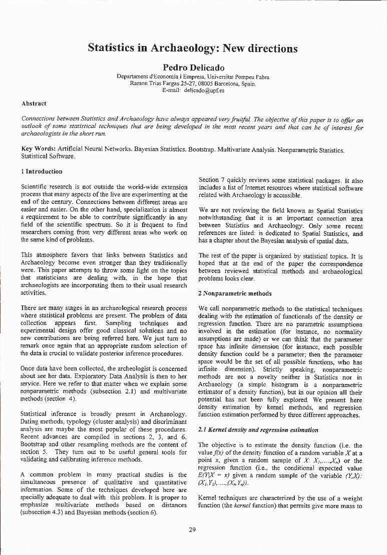
3 Artificial neural networks (ANN).

Artificial Neural Networks are very popular tools in Artificial Intelligence and Engineering. They are based on the connection of many very simple mathematical models, the artificial neurons, that imitates the work of a real neuron. We can think about an artificial neuron as a mechanism that transforms numerical input information into mmierical output information:

Inputs > -¥ Output

Output = g(Input 1,..., Input p).

The function g is an activation fiinction, that takes values near 1 for great inputs and values near 0 for low inputs.

Inputs for neuron B are the (weighted) outputs of other neurons Al,... ^p.

Outputs = gCw/OutputA I + ... + WpOutput^p),

Moreover, the output of B (modulated by some weights) is one of the inputs of (many) other neurons Cl,... ,Cq.

31

K/4^F;4 ^

LM^524

hZ2^129.5

150

•4000

Y^-rQy F.

K/i-i^^*^

\Z2i,134.5 J\0<93

-200-3300hq <13nlg1 <131.5

-400085000(200

^r^^qftS

-3300

liOiias-s

^M^53.5 ^<141.5

^1<134.5

K/4<B1.5

ia,<128.9

^103.5

„^-K^13i.5 -200-200

-185t]50-185ff

[ ] I 3z2<13<a300| Kö<ië2.5 .4odon Jb<i^

liü<:137.5 -3300

6 150

-200-1850

Figure 4. Example 2.3. CART for Egyptian skulls.

There can be a lot of these B neurons. In fact, neurons Ai and a are of the same type as B. When many neurons and many interactions are considered, we obtain an Artificial Neural Network.

As an example, we present the one hidden layer feed forward propagation ANN with a unique output. There are three neuron layers {A, ß and C) and the information goes from the fu-st layer to the second layer and then to the third one.

A B Input Hiildcn

by« layer

The strucmre of the net is as follows.

• separate external information is given to each neuron in layer A,

• gA is the identity fimction.

• gB^gc'^g,

• there is only a final neuron in layer C, and

• the information produced by layer C is return outside.

Let X, be the numerical information given to the z-th neuron in layer A and let y be the output obtained from neuron C. Then,

BC BC y = Outputc = g('wj Outputß^ +... + Wp Outputßi. ) =

/ ^, = g t wf Outputsj =

V» ; r. fp ^ \

--g Y.^fg Hwf^ Output ^1 {j=^ v'=' ;

=R [twf, ( P \

7=1 V

;=1 V ; /

This ANN is a parametric family of nonlinear fiinctions from RP to Rthat, given inputs (xi,... ,x„) returns the output value y. Each set of parameters {r.wf^.wf^} determines a different ftmction.

The fundamental property of the ANN is known as Universal approximation property and tells that every function from R P to R can be approximated by one of these one hidden layer ANNs.

32

This property originates the statistical interest for ANN. Given observations (yt, xj, i = 1,..., n, generated by the model

we can estimate <1> by means of a one hidden layer ANN.

Strictly speaking, this is a particular case of a nonlinear regression analysis. ANN literature has been developed (quite) independently and it has provided important contributions. For instance, the estimations process (or net training process) is implemented in a very different way in ANN and in nonlinear regression analysis. More connections between both topics are needed.

Statistical applications of the ANN include discriminant analysis, regression, cluster analysis and nonlinear multivariate analysis.

4 Nonlinear multivariate analysis (NLMVA)

We present here some alternative tools to the well known Principal Component Analysis and Correspondence Analysis. Some of these techniques are quite recent, but others have been introduce in the statistical literature in the 80's.

4.1 NLMVA for discrete data: The Gift system

Albert Gif! is the nom deplume for a group of authors related with the Department of Data Theory at the University of Leiden, The Netherlands. These authors compiled their work of more than 10 years in the book of Gifi (1990).

The book presents the particular idea of MVA that the Gifi team has. For instance, they affirm that all we can observe is discrete (but not all the discrete are equally rich). Moreover, no random variables are needed to be assumed the origin of data: data are enough to make Statistics.

The basic principle of the proposed techniques is the concept of homogeneity. The observed data and the observed variables are jointly transformed (in a nonlinear way) in order to obtain transformed objects as much homogeneous as possible. Not all transformation is always allowed: it depends on the data richness.

One special case of the proposed methodology is equivalent to Multiple Correspondence Analysis (MCA), but the scope of the book is wider than MCA. Continuous data can also be analyzed after a preliminary codification.

Some of the procedures developed in this book are included in the commercial package SPSS:

Principal curve for the scores on the Ppal. Cpnts. 1 and 2

-1 0 1 Score PC 1

Figure 5. Example 4.2. Principal curve for Romano-British waste glass.

4.2 NLMVA for continuous data: Principal curves

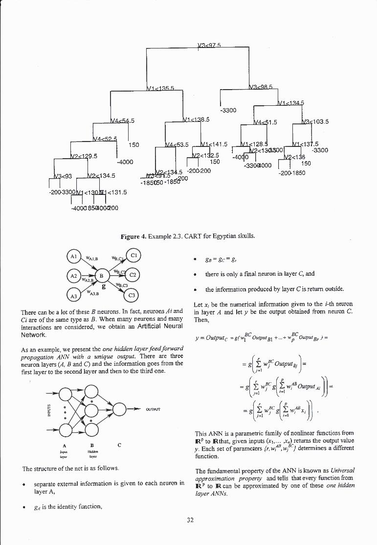
Principal curves are parameterized one dimensional curves that passe through the middle of a p-dimensional cloud of data. They are nonlinear generalizations of the first principal component. They were introduced in the work of Hastie and Stuetzle (1989). Some work has been done since then, but principal curves have not been very used, mainly because of the difficulties in the defmition and implementation for the second (and posterior) principal curves, and also because the existing associated software has not been widely diffused. Other references are LeBlanc and Tibshirani (1994), Kégl, Krzyzak, Linder and Zeger (1997), and Delicado (1998).

There exists a parallel neural network approach: Self- Organizing Maps and Generative Topographic Mapping. See, for instance, Bishop, Svensén, and Williams (1997).

Example 4

Figure 5 shows the first principal curve in the data set of the 105 glass scores on the two first principal components.

4.3 Distance based methods

We have observed/? characteristics of« objects, for instance,

Characteristic 1 ... Characteristicp Object 1 1 ... 22.5 Object 2 0 ... 29.0

• HOMALS, similar to multiple correspondence analysis, • PRINCALS, a nonlinear version of principal

components also available for ordinal data, OVERALS, a nonlinear version of canonical correlation analysis.

Object n 17.3

33

Sometimes it is easier to give a distance between objects matrix D = {dtj),

dij = Distance(Object„ Object/),

based on the p observed attributes, than proposing a joint model for these attributes.

It is possible to mix qualitative and quantitative information (Gower's distance, for instance, but there exist alternative methods).

In the last years many work has been done in order to develop usual multivariate statistical analysis (principal components, discriminant analysis, regression analysis) from a distance matrix. In the Universidad de Barcelona there is an active group of researchers in this field (see Cuadras, Fortiana, and Oliva 1997). Multidimensional scaling is a precedent to this line of work.

Talking about distances, we have to refer to cluster analysis. Alternatives to the usual hierarchical methods are the pyramidal clusters, where the resulting clusters are allowed to be overlapped. More flexibility is obtained at the prize of more difficult interpretation of the results. As a reference, see Diday (1986).

5 Bootstrap and other resampling methods

Let us assume that we are interested in a particular characteristic X of a population and that we observe the value of this variable in a sample of similar objects. For instance, X can be the volume of some cups. Let X,, ..., X„ be our observations.

We can think that each X^ is the realization of the random variable X, which has unknown distribution function Fx-

Let// = E(X) be the theoretical mean volume. Inference about ^ is based on the sample mean

M = x„=-tx^, ni=\

Confidence intervals for m can be constructed if we assume that Fx belongs to a particular parametric family and/or by means of asymptotic results. For instance, if Var(X) < oo, we know that

Sy TT A'„-L96-^,A'„+1.96 V« V«/

is an asymptotic 95% confidence interval for ;/. Let us observe that this interval has the form

where Ly, is the 2.5 percentile of the asymptotic distribution of X, and UA is its 97.5 percentile.

An alternative way to provide a confidence interval for fi could be as follows. Assume that we know Fx, so we can repeat as many times as we want the sampling process:

Sample 1

Sample N

-n; (V •X ru

X (N) ..,x (N) •X (N)

We have a size N sample of X„ from which we can build a confidence interval for // as follows,

(LN. UN).

where L^ is the 2.5 percentile of the sample X^J-* ,...,xl^^ , and Ufj is its 97.5 percentile.

The problem of this approach arises when we realize that we do not know Fx- When a statistician does not know a population characteristic, usually he or she estimates it from the data. So we estimate the theoretical distribution function Fx by the empirical distribution function F„ of our initial sample Xi,...,X„:

F„W

XI

Efron (1979) introduces the term bootstrap to designate this resampling procedure (there exist other resampling methods, as the jacknife, also covered by this book). He proposes instead of sampling from Fx, taking samples from F„, or equivalently, drawing values from the set {X,, ... X} with replacement:

Bootstrap sample 1

Bootstrap sample N

x:<'^ x'<'>^xT'

'*(N) ,...,A„ (N) x *(Nj

We resample our original sample. It is a valid procedure in many cases, but bootstrap does not always gives appropriate answers. Two are the direct advantages of bootsfrap: first, in many cases bootstrap gives better results that asymptotic arguments, and second, sometimes the only possibility to make inference is by a resampling procedure.

The scope of bootstrap methods includes,. among others, confidence intervals, hypothesis tests (as an example, see

34

Delicado and del Rio 1994) and times series. Two references are advisable: Efron and Tibshirani (1993) is a very well written book, recommended also as a very good book in Statistics; Davidson and Hinkley (1997) presents an updated review of this broad topic.

6 Bayesian methods

The Bayesian approach to Statistics is not at all new. Nevertheless we have considered appropriate to include it in this paper for several reasons. First, in the last years the Bayesian contribution to the Statistics research is dramatically increasing. Moreover, the use of powerful computers permits to give a Bayesian answer to many problems that where not accessible to Bayesian statisticians few years ago. And finally, the Bayesian methodology is not widely used in Archaeology.

Recently has appeared a book that introduces Bayesian methods to archaeological community: Buck, Cavanagh, and Litton (1996). We can read in its preface:

The major advantage of the Bayesian approach is that it allows the incorporation of relevant prior knowledge or beliefs into the analysis.

This sentence words an essential point of Bayesian Statistics.

6.1 An introduction to Bayesian methodology

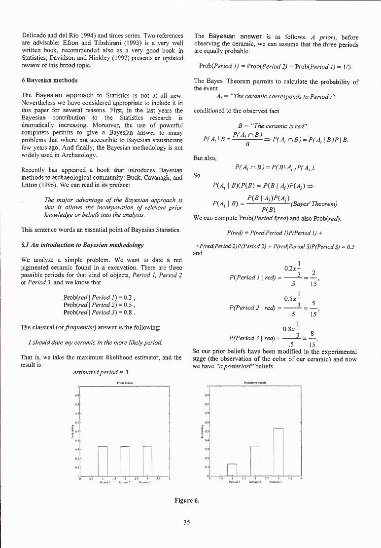
We analyze a simple problem. We want to date a red pigmented ceramic found in a excavation. There are three possible periods for that kind of objects. Period 1, Period 2 or Period 3, and we know that

PT0h(red \ Period 1) = 0.2 , ?rob{red \ Period 2) = 0.5 , Prob(rerf i Period 5) = 0.8 .

The classical (or frequentist) answer is the following:

I should date my ceramic in the more likely period.

That is, we take the maximum likelihood estimator, and the result is:

estimated period = 3.

The Bayesian answer is as follows. A priori, before observing the ceramic, we can assume that the three periods are equally probable:

Proh(Period I) = ?Tob(Period 2) = Proh(Period 1) = Ï/3.

The Bayes' Theorem permits to calculate the probability of the event

Ai = "The ceramic corresponds to Period i"

conditioned to the observed fact

P(A^ \ B =

But also,

So

B = "The ceramic is red". P(A/ n BJ

B P(AinB) = P(At\B)P\B.

P(AinB) = P(B\Ai)P(AJ.

P(Ai I B)(P{B) = P(B I 4-)^(4) =>

PiB I AAP(Af) P(A: I B) = '- '-(Bayes'Theorem)

P(B) We can compute ProhiPeriod i\red) and also PToh(red):

P(red) = P(red\Period l)P(Period 1) +

+P(red\Period 2JP(Period 2) + P(red\Period 3)P(Period 3) = 0.5 and

0.2x- 1

P(Period I | red) =

P(Period 2 \ red)

P(Period3 \red) =

.5

1 0.5x-

3

0.%x- 3

2

15^

5

8

.5 15 So our prior beliefs have been modified in the experimental stage (the observation of the color of our ceramic) and now we have "a posteriori" hsMek.

PosicrJors belicfn

Pcruiod 2 PCTOKHJ 3

Figure 6.

35

A summary of Bayesian methodology could be as follows:.

1. Prior information is expressed as a probability distribution over the parameter space.

2. Likelihood function is, in fact, the conditional distribution of the observations given the parameter values.

3. Bayes' Theorem is used to combine prior information with experimental information and transform them into posterior information: another probability distribution over the parameter space.

Some of the positive points of Bayesian Statistics are the following. Bayesian approach is concepmally appealing (and simple). For instance, the probability that a parameter belongs to a Bayesian 95% confidence interval is really 0.95. Moreover, it is possible to include prior qualitative information into the inference process. It is also possible to progressively update the beliefs: the "posterior" information of today is the "prior" information of tomorrow.

On the other hand, some difficulties are inherent in Bayesian methodology. A prior distribution is always needed, even if you do not have such "a priori" information, and some results will strongly depend on that prior. Moreover, in medium and large size problems, the computation of the posterior distribution is extremely difficult. Many times only approximate solutions are available, as the produced by the Gibbs sampling method (see subsection 6.2).

We refer to Buck, Cavanagh, and Litton (1996), pp. 208-, to follow an application example of Bayesian methods to radiocarbon dating. There, it looks clear the superiority of these techniques when qualitative information has to be included in the analysis.

6..2 Computer intensive methods

The Bayes' Theorem version for absolutely continuous random variable is:

fX(x\e)fe(9) fg(9\X^X) =

\ß(x\e)fe(e)d9'

where (X,ff) are random variables, 6 is the unobserved parameter (that can be a vector of parameters), X is observed, fx(x\q) is the likelihood function and fg(d) is the prior disn-ibution of 6. The result of the experimentation was the observation of the value x forX

In many cases, we need to solve the denominator integral (and usually this is not an easy task). In other cases, we do not want the posterior distribution of all the parameter vector, but only the posterior distribution of some parameters. For instance, 6 = (ß,cf) and we want to know the posterior distribution of m given the sample, with no attention of s. Then,

f,iM \X = x) = 1/,(//,cr I X = x)da

Again, we need to integrate.

The integration operation is usually not feasible. Then, Monte Carlo methods can help us to approximate the integrals. One of the most used Monte Carlo methods in this

area is the Gibbs sampling (see again Buck, Cavanagh, and Litton (1996)). This technique has an additional advantage: only marginal conditional distribution must be specified

f(fx\a,x)andf((7\/i,x)

instead of

7 Recommended Statistical Software

At our knowledge, no program exists implementing all the

procedures presented in this paper. Nevertheless we could list some packages.

• S-pIus. Many statistical developments are done in S- plus, and object oriented statistical commercial program that incorporates many of the most recent statistical techniques. A good book for S-plus is Venables and Ripley (1994). S-plus is possibly the most updated commercial package. It also includes a module on Spatial Statistics. Some related web sites are http://www.mathsoft.com (the official web page of S- plus) and http://www.stats.ox.ac.uk/pub/MASS.

• OxCal. Bayesian inference (including Gibbs sampling) is possible by using this package from the Oxford Radiocarbon Laboratory. It is accessible at http://units.ox.ac.uk/departments/archaeology.

• KDE: Kernel Density Estimation MATLAB toolbox, by C.C. Beardah. See also . The routines can be downloaded at ftp://ftp.maths.ntu.uk.ac/pub/ccb.

• Some other Internet resources: STATLIB (http://wwrw.stat.cmu.edu/statlib) for Statistics and S-plus.

- NEURAL CLASSIFICATION AND REGRESSION TREES. Ntree is a C library for the estimation of neural network smoothed versions of CART. (http://www.informatik.uni- freiburg.de/pub/neural/).

- NEURAL NETWORKS IN MATLAB. See the web site http://neural-server.aston.ac.uk/GTM/. GIFI SYSTEM. Source code for different compilers are available at http://www.ucla.edu/gifi/.

- PRINCIPAL CURVES. The original S-plus program from can be download at http://www.stat.cmu.edu/S/ principal.curve. Many complete information about principal curves and software related with is available at http://www.cs.concordia.ca/%7Egradykegl/research /pcurves. At http://www.econ.upf es/%7Edelicado/prcu, you can find MATLAB routines implementing the principal curves approach described in Delicado (1998).

8 Conclusions

The possibilities of interaction between Archaeology and Statistics are exfremely appealing. Joint projects of archaeologists and statisticians are certainly very promising. We borrow some words (here in italics) that Clive Orton

36

(Orton 1997) write in the review of for the Journal of Archaeological Science, and we finish the paper with a final advice:

My advice to archaeologists is bear in mind Statistics, and then be sure that you know a sympathetic statistician.

References

BAXTER, M.J. and C.C. BEARDAH (1997). Some archeological applications of kernel density estimates. Journal of Archaeological Science, 24, 347-354.

BEARDAH, C.C. and M.J. BAXTER (1995). Matlab routines for kernel density estimates and the graphical representation of archaeological data. Research Report 2/95, Nottingan Trent University, Dept. of Mathematics, Statistics and O. R.

BISHOP, C. M., M. SVENSÉN, and C. K. I. WILLIAMS (1997). GTM: A principled alternative to the self- organizing map. In Michael C. Mozer, Michael I. Jordan, and Thomas Petsche (Eds.), Advances in Neural Information Processing Systems 9, pp. 354— 360. The MIT Press.

BREIMAN, L., J.H. FRIEDMAN, R.A. OLSHEN, and C.J. STONE (1984). Classification and regression trees. Chapman and Hall.

BUCK, CE., W.G. CAVANAGH, and CD. LITTON (1996). Bayes ian Approach to Interpreting Archaeological Data. Statistics in Practice. Wiley.

CUADRAS, CM., J. FORTIANA, and F.OLIVA (1997). The proximity of an individual to a population with applications to discriminant analysis. Journal of Classification, 14, 117-136.

DAVIDSON, A.C. and D.V. HINKLEY (1997). Bootstrap Methods and their Appication. Cambridge University Press.

DELICADO, P. (1998). Another look at principal curves and surfaces. Unpublished ({\tt http://www.econ.upf es/~delicado}).

DELICADO, P. and M. del RIO (1994). Bootstrapping the general linear hypothesis test. Computational Statistics and Data Analysis, 18, 305-316.

DIDAY, E. (1986). Orders and overlapping clusters by pyramids. In J. de Leeuw, W. Heiser, J. Meulman, and F. Critchley (Eds.), Multidimensional Data Analysis, pp. 201-234. Leiden: DSWO.

EFRON, B. (1979). Bootstrap methods: another look at the jacknife. The Annals of Statistics, 1, 1-26.

EFRON, B. and R. J. TIBSHIRANI (1993). An Introduction to the Bootstrap. Chapman and Hall.

GIFI, A. (1990). Nonlinear Multivariate Analysis. Wiley. GRIFFITH, D. A. (1997). A casebook for spatial statistical

data analysis. Oxford. HASTIE, T. and W. STUETZLE (1989). Principal curves.

Journal of the American Statistical Association, 84, 502-516.

KÉGL, B., A. KRZYZAK, T. LINDER, and K. ZEGER (1997). Learning and design of principal curves. Technical Report preprint, Concordia Univ. and UC San Diego.

LeBLANC, M. and R. J. TIBSHIRANI (1994). Adaptive principal surfaces. Journal of the American Statistical Association, 89, 53-64.

MANLY, B.F.J. (1994). Multivariate Statiscal Methods. A primer. (2nd. ed.). Chapman and Hall.

ORTON, C. (1997). Review of Bayesian Approach to Interpreting Archaeological

Data (Buck et al., 1996). Journal of Archaeological Science, 24, 75.

SILVERMAN, B. (1986). Density Estimation for Statistics and Data Analysis. London: Chapman and Hall.

SIMONOFF, J.B. (1996). Smoothing methods in statistics. New York: Springer Verlag.

37