Embed Size (px)
Citation preview
15.1
STATISTICS – MEASURES OF CENTRAL TENDENCY (AVERAGES) &
DISPERSION
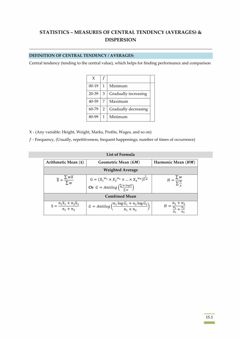
DEFINITION OF CENTRAL TENDENCY / AVERAGES:
Central tendency (tending to the central value), which helps for finding performance and comparison
X 𝑓
00-19 1 Minimum
20-39 3 Gradually increasing
40-59 7 Maximum
60-79 2 Gradually decreasing
80-99 1 Minimum
X - (Any variable: Height, Weight, Marks, Profits, Wages, and so on)
𝑓 - Frequency, (Usually, repetitiveness, frequent happenings, number of times of occurrence)
List of Formula
Arithmetic Mean (�̅�) Geometric Mean (𝑮𝑴) Harmonic Mean (𝑯𝑴)
Weighted Average
X̅ =∑ 𝑤𝑋
∑ 𝑤 G = (𝑋1
𝑤1 × 𝑋2𝑤2 × … × 𝑋𝑛
𝑤𝑛)1
∑ 𝑤
Or 𝐺 = 𝐴𝑛𝑡𝑖𝑙𝑜𝑔 (∑ 𝑤 𝑙𝑜𝑔𝑋
∑ 𝑤)
𝐻 =∑ 𝑤
∑𝑤
𝑋
Combined Mean
x̅ =𝑛1x̅1 + 𝑛2x̅2
𝑛1 + 𝑛2
𝐺 = 𝐴𝑛𝑡𝑖𝑙𝑜𝑔 (𝑛1 log 𝐺1 + 𝑛2 log 𝐺2
𝑛1 + 𝑛2
) 𝐻 =𝑛1 + 𝑛2𝑛1
𝐻1+
𝑛2
𝐻2
15.2
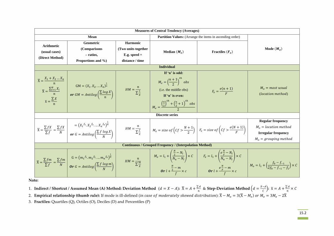
Measures of Central Tendency (Averages)
Mean Partition Values: (Arrange the items in ascending order)
Mode (𝑴𝒐) Arithmetic
(usual cases)
(Direct Method)
Geometric
(Comparisons
– ratios,
Proportions and %)
Harmonic
(Two units together
E.g. speed =
distance / time
Median (𝑴𝒆) Fractiles (𝑭𝒆)
Individual
X̅ =𝑋1 + 𝑋2 … 𝑋𝑛
𝑛
X̅ =∑ 𝑋𝑖
𝑁𝑖=1
𝑛
x̅ =∑ 𝑋
𝑛
GM = (𝑋1. 𝑋2. … 𝑋𝑛)1
𝑛
𝒐𝒓 𝐺𝑀 = 𝐴𝑛𝑡𝑖𝑙𝑜𝑔 (∑ 𝑙𝑜𝑔 𝑋
𝑛)
𝐻𝑀 =𝑛
∑1
𝑋
If ‘n’ is odd:
𝑀𝑒 = (𝑛 + 1
2)
𝑡ℎ
𝑜𝑏𝑠
(i.e. the middle obs)
If ‘n’ is even:
𝑀𝑒 =(
𝑛
2)
𝑡ℎ+ (
𝑛
2+ 1)
𝑡ℎ 𝑜𝑏𝑠
2
𝐹𝑒 =𝑒(𝑛 + 1)
𝐹
𝑀𝑜 = 𝑚𝑜𝑠𝑡 𝑢𝑠𝑢𝑎𝑙
(𝑙𝑜𝑐𝑎𝑡𝑖𝑜𝑛 𝑚𝑒𝑡ℎ𝑜𝑑)
Discrete series
X̅ =∑ 𝑓𝑋
∑ 𝑓 =
∑ 𝑓𝑋
𝑁
= (𝑋1𝑓1 . 𝑋2
𝑓2 . … 𝑋𝑛𝑓𝑛)
1
𝑁
𝒐𝒓 𝐺 = 𝐴𝑛𝑡𝑖𝑙𝑜𝑔 (∑ 𝑓 𝑙𝑜𝑔 𝑋
𝑁)
𝐻𝑀 =𝑛
∑𝑓
𝑋
𝑀𝑒 = 𝑠𝑖𝑧𝑒 𝑜𝑓 (𝐶𝑓 >𝑁 + 1
2) 𝐹𝑒 = 𝑠𝑖𝑧𝑒 𝑜𝑓 (𝐶𝑓 >
𝑒(𝑁 + 1)
𝐹)
Regular frequency
𝑀𝑜 = 𝑙𝑜𝑐𝑎𝑡𝑖𝑜𝑛 𝑚𝑒𝑡ℎ𝑜𝑑
Irregular frequency
𝑀𝑜 = 𝑔𝑟𝑜𝑢𝑝𝑖𝑛𝑔 𝑚𝑒𝑡ℎ𝑜𝑑
Continuous / Grouped Frequency / (Interpolation Method)
X̅ =∑ 𝑓𝑚
∑ 𝑓 =
∑ 𝑓𝑚
𝑁
G = (𝑚1𝑓1 . 𝑚2
𝑓2 . … 𝑚𝑛𝑓𝑛)
1
𝑁
𝑶𝒓 𝐺 = 𝐴𝑛𝑡𝑖𝑙𝑜𝑔 (∑ 𝑓 𝑙𝑜𝑔 𝑚
𝑁)
𝐻𝑀 =𝑛
∑𝑚
𝑋
𝑀𝑒 = 𝑙1 + (
𝑁
2− 𝑁𝑙
𝑁𝑢 − 𝑁𝑙) × 𝐶
𝑶𝒓 𝑙 +
𝑁
2− 𝑚
𝑓× 𝑐
𝐹𝑒 = 𝑙1 + (𝑒
𝑁
𝐹− 𝑁𝑙
𝑁𝑢 − 𝑁𝑙) × 𝐶
𝑶𝒓 𝑙 +𝑒
𝑁
𝐹− 𝑚
𝑓× 𝑐
𝑀𝑜 = 𝑙1 + (𝑓0 − 𝑓−1
2𝑓0 − 𝑓−1 − 𝑓1) × 𝐶
Note:
1. Indirect / Shortcut / Assumed Mean (A) Method: Deviation Method (𝑑 = 𝑋 − 𝐴): X̅ = 𝐴 +∑ 𝑑
𝑛 & Step-Deviation Method (𝑑 =
𝑋−𝐴
𝐶): x̅ = 𝐴 +
∑ 𝑑
𝑛× 𝐶
2. Empirical relationship (thumb rule): If mode is ill-defined (𝑖𝑛 𝑐𝑎𝑠𝑒 𝑜𝑓 𝑚𝑜𝑑𝑒𝑟𝑎𝑡𝑒𝑙𝑦 𝑠𝑘𝑒𝑤𝑒𝑑 𝑑𝑖𝑠𝑡𝑟𝑖𝑏𝑢𝑡𝑖𝑜𝑛): X̅ − 𝑀𝑜 = 3(X̅ − 𝑀𝑒) 𝑜𝑟 𝑀𝑜 = 3𝑀𝑒 − 2X̅
3. Fractiles: Quartiles (Q), Octiles (O), Deciles (D) and Percentiles (P)
15.3
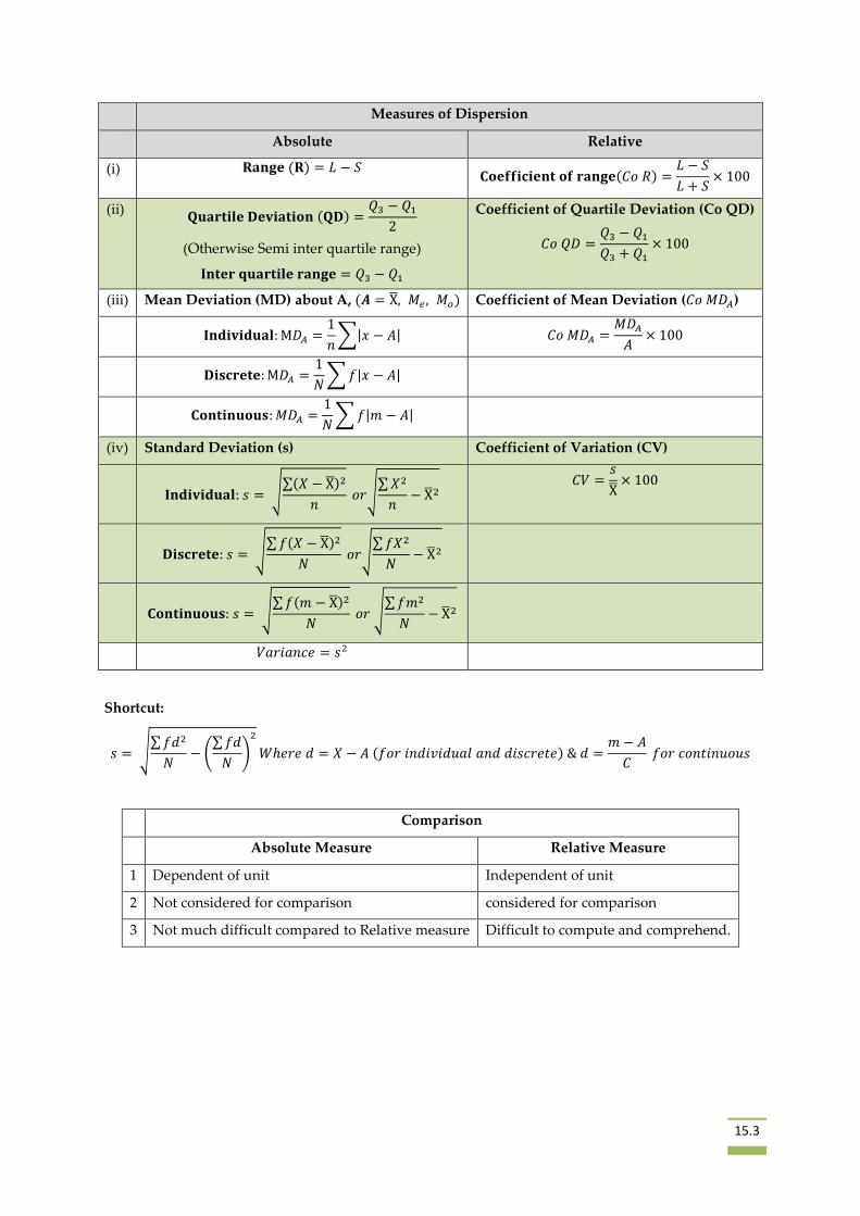
Measures of Dispersion
Absolute Relative
(i) 𝐑𝐚𝐧𝐠𝐞 (𝐑) = 𝐿 − 𝑆 𝐂𝐨𝐞𝐟𝐟𝐢𝐜𝐢𝐞𝐧𝐭 𝐨𝐟 𝐫𝐚𝐧𝐠𝐞(𝐶𝑜 𝑅) =
𝐿 − 𝑆
𝐿 + 𝑆× 100
(ii) 𝐐𝐮𝐚𝐫𝐭𝐢𝐥𝐞 𝐃𝐞𝐯𝐢𝐚𝐭𝐢𝐨𝐧 (𝐐𝐃) =
𝑄3 − 𝑄1
2
(Otherwise Semi inter quartile range)
𝐈𝐧𝐭𝐞𝐫 𝐪𝐮𝐚𝐫𝐭𝐢𝐥𝐞 𝐫𝐚𝐧𝐠𝐞 = 𝑄3 − 𝑄1
Coefficient of Quartile Deviation (Co QD)
𝐶𝑜 𝑄𝐷 =𝑄3 − 𝑄1
𝑄3 + 𝑄1
× 100
(iii) Mean Deviation (MD) about A, (𝑨 = X̅, 𝑀𝑒 , 𝑀𝑜) Coefficient of Mean Deviation (𝐶𝑜 𝑀𝐷𝐴)
𝐈𝐧𝐝𝐢𝐯𝐢𝐝𝐮𝐚𝐥: M𝐷𝐴 =
1
𝑛∑|𝑥 − 𝐴| 𝐶𝑜 𝑀𝐷𝐴 =
𝑀𝐷𝐴
𝐴× 100
𝐃𝐢𝐬𝐜𝐫𝐞𝐭𝐞: M𝐷𝐴 =
1
𝑁∑ 𝑓|𝑥 − 𝐴|
𝐂𝐨𝐧𝐭𝐢𝐧𝐮𝐨𝐮𝐬: 𝑀𝐷𝐴 =
1
𝑁∑ 𝑓|𝑚 − 𝐴|
(iv) Standard Deviation (s) Coefficient of Variation (CV)
𝐈𝐧𝐝𝐢𝐯𝐢𝐝𝐮𝐚𝐥: 𝑠 = √∑(𝑋 − X̅)2
𝑛 𝑜𝑟√
∑ 𝑋2
𝑛− X̅2
𝐶𝑉 =𝑠
X̅× 100
𝐃𝐢𝐬𝐜𝐫𝐞𝐭𝐞: 𝑠 = √∑ 𝑓(𝑋 − X̅)2
𝑁 𝑜𝑟√
∑ 𝑓𝑋2
𝑁− X̅2
𝐂𝐨𝐧𝐭𝐢𝐧𝐮𝐨𝐮𝐬: 𝑠 = √∑ 𝑓(𝑚 − X̅)2
𝑁 𝑜𝑟 √
∑ 𝑓𝑚2
𝑁− X̅2
𝑉𝑎𝑟𝑖𝑎𝑛𝑐𝑒 = 𝑠2
Shortcut:
𝑠 = √∑ 𝑓𝑑2
𝑁− (
∑ 𝑓𝑑
𝑁)
2
𝑊ℎ𝑒𝑟𝑒 𝑑 = 𝑋 − 𝐴 (𝑓𝑜𝑟 𝑖𝑛𝑑𝑖𝑣𝑖𝑑𝑢𝑎𝑙 𝑎𝑛𝑑 𝑑𝑖𝑠𝑐𝑟𝑒𝑡𝑒) & 𝑑 =𝑚 − 𝐴
𝐶 𝑓𝑜𝑟 𝑐𝑜𝑛𝑡𝑖𝑛𝑢𝑜𝑢𝑠
Comparison
Absolute Measure Relative Measure
1 Dependent of unit Independent of unit
2 Not considered for comparison considered for comparison
3 Not much difficult compared to Relative measure Difficult to compute and comprehend.
15.4
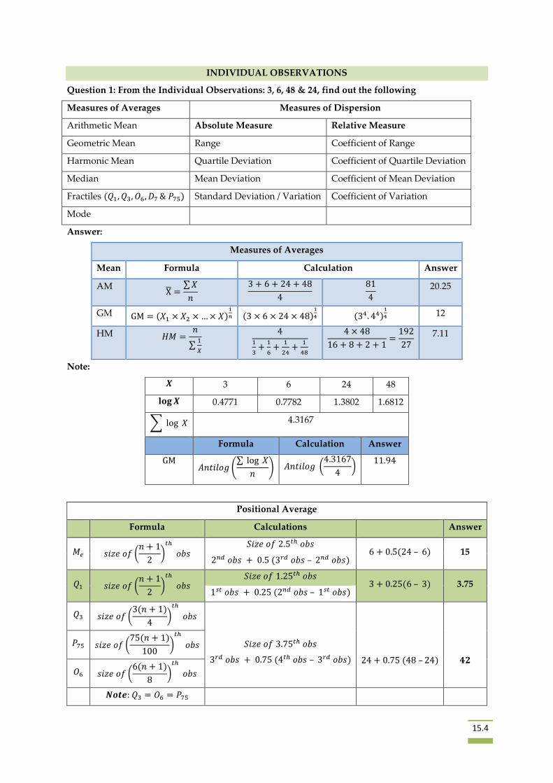
INDIVIDUAL OBSERVATIONS
Question 1: From the Individual Observations: 3, 6, 48 & 24, find out the following
Measures of Averages Measures of Dispersion
Arithmetic Mean Absolute Measure Relative Measure
Geometric Mean Range Coefficient of Range
Harmonic Mean Quartile Deviation Coefficient of Quartile Deviation
Median Mean Deviation Coefficient of Mean Deviation
Fractiles (𝑄1, 𝑄3, 𝑂6, 𝐷7 & 𝑃75) Standard Deviation / Variation Coefficient of Variation
Mode
Answer:
Measures of Averages
Mean Formula Calculation Answer
AM X̅ =
∑ 𝑋
𝑛
3 + 6 + 24 + 48
4
81
4
20.25
GM GM = (𝑋1 × 𝑋2 × … × 𝑋)1
𝑛 (3 × 6 × 24 × 48)1
4 (34. 44)1
4 12
HM 𝐻𝑀 =𝑛
∑1
𝑋
4
1
3+
1
6+
1
24+
1
48
4 × 48
16 + 8 + 2 + 1=
192
27
7.11
Note:
𝑿 3 6 24 48
𝐥𝐨𝐠 𝑿 0.4771 0.7782 1.3802 1.6812
∑ log 𝑋 4.3167
Formula Calculation Answer
GM 𝐴𝑛𝑡𝑖𝑙𝑜𝑔 (
∑ log 𝑋
𝑛) 𝐴𝑛𝑡𝑖𝑙𝑜𝑔 (
4.3167
4)
11.94
Positional Average
Formula Calculations Answer
𝑀𝑒 𝑠𝑖𝑧𝑒 𝑜𝑓 (𝑛 + 1
2)
𝑡ℎ
𝑜𝑏𝑠 𝑆𝑖𝑧𝑒 𝑜𝑓 2.5𝑡ℎ 𝑜𝑏𝑠
6 + 0.5(24 – 6) 15 2𝑛𝑑 𝑜𝑏𝑠 + 0.5 (3𝑟𝑑 𝑜𝑏𝑠 – 2𝑛𝑑 𝑜𝑏𝑠)
𝑄1 𝑠𝑖𝑧𝑒 𝑜𝑓 (𝑛 + 1
2)
𝑡ℎ
𝑜𝑏𝑠 𝑆𝑖𝑧𝑒 𝑜𝑓 1.25𝑡ℎ 𝑜𝑏𝑠
3 + 0.25(6 – 3) 3.75 1𝑠𝑡 𝑜𝑏𝑠 + 0.25 (2𝑛𝑑 𝑜𝑏𝑠 – 1𝑠𝑡 𝑜𝑏𝑠)
𝑄3 𝑠𝑖𝑧𝑒 𝑜𝑓 (3(𝑛 + 1)
4)
𝑡ℎ
𝑜𝑏𝑠
𝑆𝑖𝑧𝑒 𝑜𝑓 3.75𝑡ℎ 𝑜𝑏𝑠
3𝑟𝑑 𝑜𝑏𝑠 + 0.75 (4𝑡ℎ 𝑜𝑏𝑠 – 3𝑟𝑑 𝑜𝑏𝑠)
24 + 0.75 (48 – 24)
𝟒𝟐
𝑃75 𝑠𝑖𝑧𝑒 𝑜𝑓 (75(𝑛 + 1)
100)
𝑡ℎ
𝑜𝑏𝑠
𝑂6 𝑠𝑖𝑧𝑒 𝑜𝑓 (6(𝑛 + 1)
8)
𝑡ℎ
𝑜𝑏𝑠
𝑵𝒐𝒕𝒆: 𝑄3 = 𝑂6 = 𝑃75
15.5
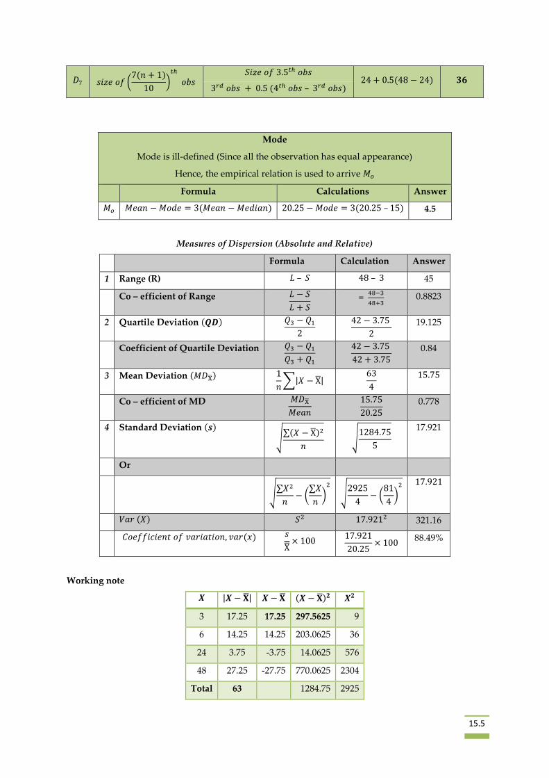
𝐷7 𝑠𝑖𝑧𝑒 𝑜𝑓 (7(𝑛 + 1)
10)
𝑡ℎ
𝑜𝑏𝑠 𝑆𝑖𝑧𝑒 𝑜𝑓 3.5𝑡ℎ 𝑜𝑏𝑠
24 + 0.5(48 − 24) 𝟑𝟔 3𝑟𝑑 𝑜𝑏𝑠 + 0.5 (4𝑡ℎ 𝑜𝑏𝑠 – 3𝑟𝑑 𝑜𝑏𝑠)
Mode
Mode is ill-defined (Since all the observation has equal appearance)
Hence, the empirical relation is used to arrive 𝑀𝑜
Formula Calculations Answer
𝑀𝑜 𝑀𝑒𝑎𝑛 − 𝑀𝑜𝑑𝑒 = 3(𝑀𝑒𝑎𝑛 − 𝑀𝑒𝑑𝑖𝑎𝑛) 20.25 − 𝑀𝑜𝑑𝑒 = 3(20.25 – 15) 4.5
Measures of Dispersion (Absolute and Relative)
Formula Calculation Answer
1 Range (R) 𝐿 – 𝑆 48 – 3 45
Co – efficient of Range 𝐿 − 𝑆
𝐿 + 𝑆 =
48−3
48+3 0.8823
2 Quartile Deviation (𝑸𝑫) 𝑄3 − 𝑄1
2
42 − 3.75
2
19.125
Coefficient of Quartile Deviation 𝑄3 − 𝑄1
𝑄3 + 𝑄1
42 − 3.75
42 + 3.75
0.84
3 Mean Deviation (𝑀𝐷X̅) 1
𝑛∑|𝑋 − X̅|
63
4
15.75
Co – efficient of MD 𝑀𝐷X̅
𝑀𝑒𝑎𝑛
15.75
20.25
0.778
4 Standard Deviation (𝒔) √
∑(𝑋 − X̅)2
𝑛 √
1284.75
5
17.921
Or
√
∑𝑋2
𝑛− (
∑𝑋
𝑛)
2
√2925
4− (
81
4)
2
17.921
𝑉𝑎𝑟 (𝑋) 𝑆2 17.9212 321.16
𝐶𝑜𝑒𝑓𝑓𝑖𝑐𝑖𝑒𝑛𝑡 𝑜𝑓 𝑣𝑎𝑟𝑖𝑎𝑡𝑖𝑜𝑛, 𝑣𝑎𝑟(𝑥) 𝑠
X̅× 100
17.921
20.25× 100
88.49%
Working note
𝑿 |𝑿 − �̅�| 𝑿 − 𝐗 (𝑿 − �̅�)𝟐 𝑿𝟐
3 17.25 17.25 297.5625 9
6 14.25 14.25 203.0625 36
24 3.75 -3.75 14.0625 576
48 27.25 -27.75 770.0625 2304
Total 63 1284.75 2925

15.6
Question 2: Find Median, 𝑸𝟏, 𝑸𝟑,𝑶𝟔, 𝑫𝟕, 𝑷𝟕𝟓 for the observations: 1, 3, 6, 24, 48.
Answer:
Positional Average
Formula Calculations Answer
𝑀𝑒 𝑠𝑖𝑧𝑒 𝑜𝑓 (
𝑛 + 1
2)
𝑡ℎ
𝑜𝑏𝑠 𝑆𝑖𝑧𝑒 𝑜𝑓 3𝑟𝑑 𝑜𝑏𝑠 6 + 0.5(24 – 6) 6
𝑄1 𝑠𝑖𝑧𝑒 𝑜𝑓 (
𝑛 + 1
4)
𝑡ℎ
𝑜𝑏𝑠 𝑆𝑖𝑧𝑒 𝑜𝑓 1.5𝑡ℎ 𝑜𝑏𝑠 1 + 0.5(3 – 1) 2
1𝑠𝑡 𝑜𝑏𝑠 + 0.5 (2𝑛𝑑 𝑜𝑏𝑠 – 1𝑠𝑡 𝑜𝑏𝑠)
𝑄3 𝑠𝑖𝑧𝑒 𝑜𝑓 (
3(𝑛 + 1)
4)
𝑡ℎ
𝑜𝑏𝑠
𝑆𝑖𝑧𝑒 𝑜𝑓 4.5𝑡ℎ 𝑜𝑏𝑠
4𝑡ℎ 𝑜𝑏𝑠 + 0.5 (5𝑡ℎ 𝑜𝑏𝑠 – 4𝑡ℎ 𝑜𝑏𝑠)
24 + 0.5 (48 – 24)
36 𝑃75
𝑠𝑖𝑧𝑒 𝑜𝑓 (75(𝑛 + 1)
100)
𝑡ℎ
𝑜𝑏𝑠
𝑂6 𝑠𝑖𝑧𝑒 𝑜𝑓 (
6(𝑛 + 1)
8)
𝑡ℎ
𝑜𝑏𝑠
𝑵𝒐𝒕𝒆: 𝑄3 = 𝑂6 = 𝑃75
𝐷7 𝑠𝑖𝑧𝑒 𝑜𝑓 (
7(𝑛 + 1)
10)
𝑡ℎ
𝑜𝑏𝑠 𝑆𝑖𝑧𝑒 𝑜𝑓 4.2𝑡ℎ 𝑜𝑏𝑠 24 + 0.2(48 − 24) 𝟐𝟖. 𝟖
4𝑡ℎ 𝑜𝑏𝑠 + 0.2 (5𝑡ℎ 𝑜𝑏𝑠 – 4𝑡ℎ 𝑜𝑏𝑠)
Question 3: Discrete Frequency Distribution
x 10 11 12 13 14 15 16 17 18 19
f 8 15 20 100 98 95 90 75 50 30
Answer:
Measures of Averages
Formula Calculation Answer
1 Arithmetic Mean(x̅) ∑𝑓𝑋
𝑁
8727
581 15.02
2 Geometric Mean(𝐺𝑀) Antilog (∑ 𝑓 log 𝑋
𝑁) Antilog (
682.4203
581) 14.95
3 Harmonic Mean (𝐻𝑀) 𝑁
∑𝑓
𝑋
581
39.25 14.802
Working Note:
𝑿 𝒇 𝒇𝑿 𝐥𝐨𝐠 𝑿 𝒇 𝐥𝐨𝐠 𝑿 𝒇
𝑿
10 8 80 1.0000 8.0000 0.800
11 15 165 1.0414 15.6210 1.360
12 20 240 1.0792 21.5840 1.670
13 100 1300 1.1139 111.3900 7.690

15.7
14 98 1372 1.1461 112.3178 7.000
15 95 1425 1.1761 111.7295 6.330
16 90 1440 1.2041 108.3690 5.625
17 75 1275 1.2304 92.2800 4.411
18 50 900 1.2553 62.7650 2.780
19 30 570 1.2788 38.364 1.578
Total 581 8727 682.4203 39.25
Positional Average
Formula Calculations Answer Working Notes
𝑀𝑒 𝑠𝑖𝑧𝑒 𝑜𝑓 (𝑁 + 1
2)
𝑡ℎ
𝑜𝑏𝑠 𝑆𝑖𝑧𝑒 𝑜𝑓 291𝑠𝑡 𝑜𝑏𝑠
(𝑖. 𝑒. 𝑐𝑓 > 291) 15
𝑿 𝑓 𝑐𝑓
10 8 8
11 15 23
12 20 43
13 100 143
14 98 241
15 95 336
16 90 426
17 75 501
18 50 551
19 30 581
𝑄1 𝑠𝑖𝑧𝑒 𝑜𝑓 (1(𝑁 + 1)
4)
𝑡ℎ
𝑜𝑏𝑠 𝑆𝑖𝑧𝑒 𝑜𝑓 145.5𝑡ℎ 𝑜𝑏𝑠
(𝑖. 𝑒. 𝑐𝑓 > 145.5) 14
𝑄3 𝑠𝑖𝑧𝑒 𝑜𝑓 (3(𝑁 + 1)
4)
𝑡ℎ
𝑜𝑏𝑠
𝑆𝑖𝑧𝑒 𝑜𝑓 436.5𝑡ℎ 𝑜𝑏𝑠
(𝑖. 𝑒. 𝑐𝑓 > 436.5)
17
𝑃75 𝑠𝑖𝑧𝑒 𝑜𝑓 (75(𝑁 + 1)
100)
𝑡ℎ
𝑜𝑏𝑠
𝑂6 𝑠𝑖𝑧𝑒 𝑜𝑓 (6(𝑁 + 1)
8)
𝑡ℎ
𝑜𝑏𝑠
𝑵𝒐𝒕𝒆: 𝑄3 = 𝑂6 = 𝑃75
𝐷7 𝑠𝑖𝑧𝑒 𝑜𝑓 (7(𝑁 + 1)
10)
𝑡ℎ
𝑜𝑏𝑠 𝑆𝑖𝑧𝑒 𝑜𝑓 407.4𝑡ℎ 𝑜𝑏𝑠
𝟏𝟔 (𝑖. 𝑒. 𝑐𝑓 > 407.4)
Mode: Since there is a sudden increase in frequency from 20 to 100, we obtain mode by Grouping
Table
Grouping Table The highest frequency total in each of the six
columns of the grouping table is identified and
analyzed (Tally marks)
Total
Tally
Mark
(1) (2) (3) (4) (5) (6)
𝑿 𝒇 (1) (2) (3) (4) (5) (6)
10 8 23
43
0
11 15 35
135
0
12 20 120
218
0
13 100 198
293
| | | 3
14 98 193
283
| | | | 4
15 95 185
260
| | | | 4
16 90 165
215
| | 2
17 75 125
155
| 1
18 50 80
0
19 30 0
15.8
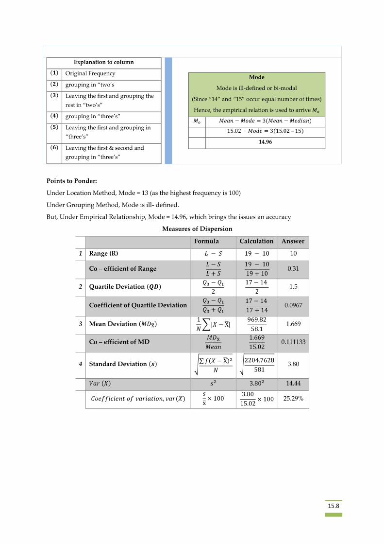
Explanation to column
(𝟏) Original Frequency
(𝟐) grouping in “two’s
(𝟑) Leaving the first and grouping the
rest in “two’s”
(𝟒) grouping in “three’s”
(𝟓) Leaving the first and grouping in
“three’s”
(𝟔) Leaving the first & second and
grouping in “three’s”
Mode
Mode is ill-defined or bi-modal
(Since “14” and “15” occur equal number of times)
Hence, the empirical relation is used to arrive 𝑀𝑜
𝑀𝑜 𝑀𝑒𝑎𝑛 − 𝑀𝑜𝑑𝑒 = 3(𝑀𝑒𝑎𝑛 − 𝑀𝑒𝑑𝑖𝑎𝑛)
15.02 − 𝑀𝑜𝑑𝑒 = 3(15.02 – 15)
14.96
Points to Ponder:
Under Location Method, Mode = 13 (as the highest frequency is 100)
Under Grouping Method, Mode is ill- defined.
But, Under Empirical Relationship, Mode = 14.96, which brings the issues an accuracy
Measures of Dispersion
Formula Calculation Answer
1 Range (R) 𝐿 − 𝑆 19 − 10 10
Co – efficient of Range 𝐿 − 𝑆
𝐿 + 𝑆
19 − 10
19 + 10 0.31
2 Quartile Deviation (𝑸𝑫) 𝑄3 − 𝑄1
2
17 − 14
2 1.5
Coefficient of Quartile Deviation 𝑄3 − 𝑄1
𝑄3 + 𝑄1
17 − 14
17 + 14 0.0967
3 Mean Deviation (𝑀𝐷X̅) 1
𝑁∑|𝑋 − X̅|
969.82
58.1 1.669
Co – efficient of MD 𝑀𝐷X̅
𝑀𝑒𝑎𝑛
1.669
15.02 0.111133
4 Standard Deviation (𝒔) √∑ 𝑓(𝑋 − X̅)2
𝑁 √
2204.7628
581 3.80
𝑉𝑎𝑟 (𝑋) 𝑠2 3.802 14.44
𝐶𝑜𝑒𝑓𝑓𝑖𝑐𝑖𝑒𝑛𝑡 𝑜𝑓 𝑣𝑎𝑟𝑖𝑎𝑡𝑖𝑜𝑛, 𝑣𝑎𝑟(𝑋) 𝑠
x̅× 100
3.80
15.02× 100 25.29%
15.9
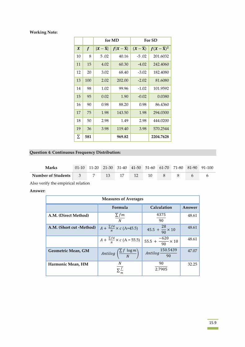
Working Note:
for MD For SD
𝑿 𝒇 |𝑿 − �̅�| 𝒇|𝑿 − 𝐗| (𝑿 − �̅�) 𝒇(𝑿 − �̅�)𝟐
10 8 5 .02 40.16 -5 .02 201.6032
11 15 4.02 60.30 -4.02 242.4060
12 20 3.02 68.40 -3.02 182.4080
13 100 2.02 202.00 -2.02 81.6080
14 98 1.02 99.96 -1.02 101.9592
15 95 0.02 1.90 -0.02 0.0380
16 90 0.98 88.20 0.98 86.4360
17 75 1.98 143.50 1.98 294.0300
18 50 2.98 1.49 2.98 444.0200
19 36 3.98 119.40 3.98 570.2544
∑ 581 969.82 2204.7628
Question 4: Continuous Frequency Distribution:
Marks 01-10 11-20 21-30 31-40 41-50 51-60 61-70 71-80 81-90 91-100
Number of Students 3 7 13 17 12 10 8 8 6 6
Also verify the empirical relation
Answer:
Measures of Averages
Formula Calculation Answer
A.M. (Direct Method) ∑ 𝑓𝑚
𝑁
4375
90
48.61
A.M. (Short cut -Method) 𝐴 + ∑ 𝑓𝑑
𝑁× 𝑐 (A=45.5) 45.5 +
28
90× 10
48.61
𝐴 + ∑ 𝑓𝑑
𝑁× 𝑐 (A = 55.5) 55.5 +
−620
90× 10
48.61
Geometric Mean, GM 𝐴𝑛𝑡𝑖𝑙𝑜𝑔 (
∑ 𝑓 log 𝑚
𝑁) 𝐴𝑛𝑡𝑖𝑙𝑜𝑔
150.5439
90
47.07
Harmonic Mean, HM 𝑁
∑𝑓
𝑚
90
2.7905
32.25
15.10
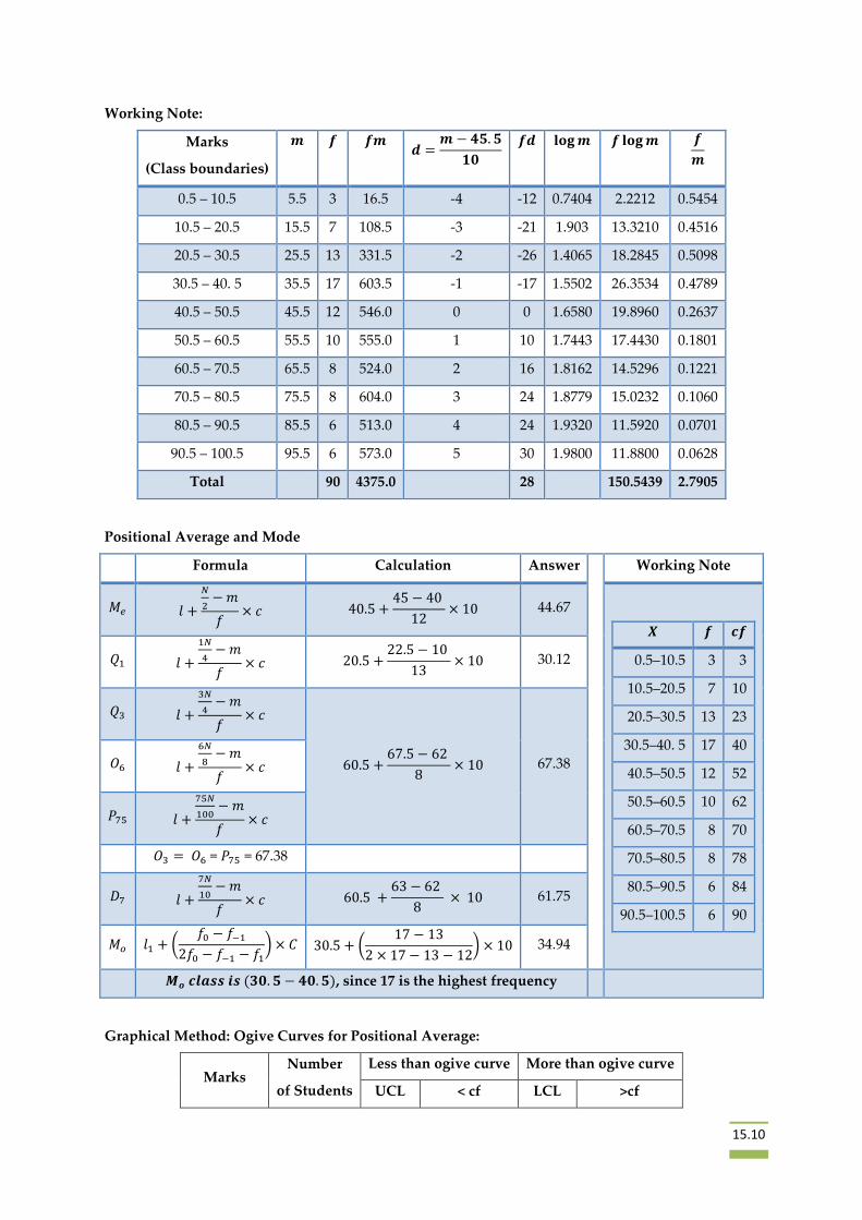
Working Note:
Marks
(Class boundaries)
𝒎 𝒇 𝒇𝒎 𝒅 =
𝒎 − 𝟒𝟓. 𝟓
𝟏𝟎
𝒇𝒅 𝐥𝐨𝐠 𝒎 𝒇 𝐥𝐨𝐠 𝒎 𝒇
𝒎
0.5 – 10.5 5.5 3 16.5 -4 -12 0.7404 2.2212 0.5454
10.5 – 20.5 15.5 7 108.5 -3 -21 1.903 13.3210 0.4516
20.5 – 30.5 25.5 13 331.5 -2 -26 1.4065 18.2845 0.5098
30.5 – 40. 5 35.5 17 603.5 -1 -17 1.5502 26.3534 0.4789
40.5 – 50.5 45.5 12 546.0 0 0 1.6580 19.8960 0.2637
50.5 – 60.5 55.5 10 555.0 1 10 1.7443 17.4430 0.1801
60.5 – 70.5 65.5 8 524.0 2 16 1.8162 14.5296 0.1221
70.5 – 80.5 75.5 8 604.0 3 24 1.8779 15.0232 0.1060
80.5 – 90.5 85.5 6 513.0 4 24 1.9320 11.5920 0.0701
90.5 – 100.5 95.5 6 573.0 5 30 1.9800 11.8800 0.0628
Total 90 4375.0 28 150.5439 2.7905
Positional Average and Mode
Formula Calculation Answer
Working Note
𝑀𝑒 𝑙 +
𝑁
2− 𝑚
𝑓× 𝑐 40.5 +
45 − 40
12× 10 44.67
𝑿 𝒇 𝒄𝒇
0.5–10.5 3 3
10.5–20.5 7 10
20.5–30.5 13 23
30.5–40. 5 17 40
40.5–50.5 12 52
50.5–60.5 10 62
60.5–70.5 8 70
70.5–80.5 8 78
80.5–90.5 6 84
90.5–100.5 6 90
𝑄1 𝑙 +
1𝑁
4− 𝑚
𝑓× 𝑐 20.5 +
22.5 − 10
13× 10 30.12
𝑄3 𝑙 +
3𝑁
4− 𝑚
𝑓× 𝑐
60.5 +67.5 − 62
8× 10 67.38 𝑂6 𝑙 +
6𝑁
8− 𝑚
𝑓× 𝑐
𝑃75 𝑙 +
75𝑁
100− 𝑚
𝑓× 𝑐
𝑂3 = 𝑂6 = 𝑃75 = 67.38
𝐷7 𝑙 +
7𝑁
10− 𝑚
𝑓× 𝑐 60.5 +
63 − 62
8 × 10 61.75
𝑀𝑜 𝑙1 + (𝑓0 − 𝑓−1
2𝑓0 − 𝑓−1 − 𝑓1
) × 𝐶 30.5 + (17 − 13
2 × 17 − 13 − 12) × 10 34.94
𝑴𝒐 𝒄𝒍𝒂𝒔𝒔 𝒊𝒔 (𝟑𝟎. 𝟓 − 𝟒𝟎. 𝟓), since 17 is the highest frequency
Graphical Method: Ogive Curves for Positional Average:
Marks Number
of Students
Less than ogive curve More than ogive curve
UCL < cf LCL >cf
15.11
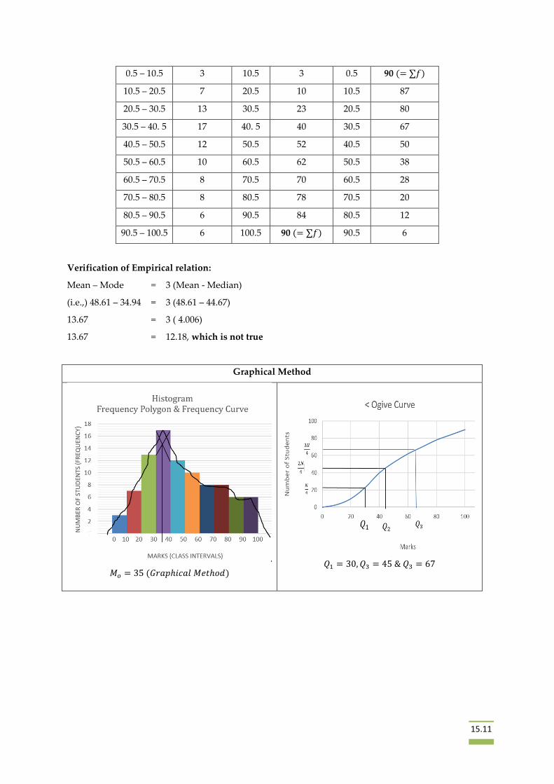
0.5 – 10.5 3 10.5 3 0.5 90 (= ∑𝑓)
10.5 – 20.5 7 20.5 10 10.5 87
20.5 – 30.5 13 30.5 23 20.5 80
30.5 – 40. 5 17 40. 5 40 30.5 67
40.5 – 50.5 12 50.5 52 40.5 50
50.5 – 60.5 10 60.5 62 50.5 38
60.5 – 70.5 8 70.5 70 60.5 28
70.5 – 80.5 8 80.5 78 70.5 20
80.5 – 90.5 6 90.5 84 80.5 12
90.5 – 100.5 6 100.5 90 (= ∑𝑓) 90.5 6
Verification of Empirical relation:
Mean – Mode = 3 (Mean - Median)
(i.e.,) 48.61 – 34.94 = 3 (48.61 – 44.67)
13.67 = 3 ( 4.006)
13.67 = 12.18, which is not true
Graphical Method
𝑀𝑜 = 35 (𝐺𝑟𝑎𝑝ℎ𝑖𝑐𝑎𝑙 𝑀𝑒𝑡ℎ𝑜𝑑)
𝑄1 = 30, 𝑄3 = 45 & 𝑄3 = 67
15.12
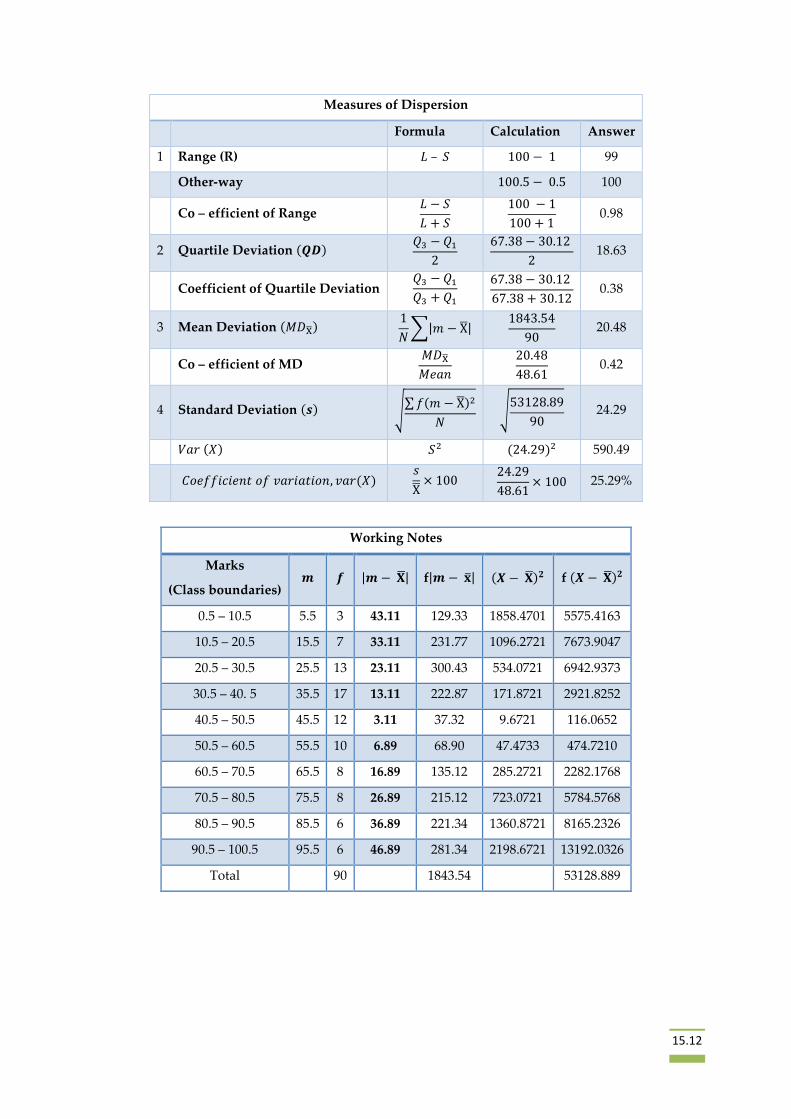
Measures of Dispersion
Formula Calculation Answer
1 Range (R) 𝐿 – 𝑆 100 − 1 99
Other-way 100.5 − 0.5 100
Co – efficient of Range 𝐿 − 𝑆
𝐿 + 𝑆
100 − 1
100 + 1 0.98
2 Quartile Deviation (𝑸𝑫) 𝑄3 − 𝑄1
2
67.38 − 30.12
2 18.63
Coefficient of Quartile Deviation 𝑄3 − 𝑄1
𝑄3 + 𝑄1
67.38 − 30.12
67.38 + 30.12 0.38
3 Mean Deviation (𝑀𝐷X̅) 1
𝑁∑|𝑚 − X̅|
1843.54
90 20.48
Co – efficient of MD 𝑀𝐷X̅
𝑀𝑒𝑎𝑛
20.48
48.61 0.42
4 Standard Deviation (𝒔) √∑ 𝑓(𝑚 − X̅)2
𝑁 √
53128.89
90 24.29
𝑉𝑎𝑟 (𝑋) 𝑆2 (24.29)2 590.49
𝐶𝑜𝑒𝑓𝑓𝑖𝑐𝑖𝑒𝑛𝑡 𝑜𝑓 𝑣𝑎𝑟𝑖𝑎𝑡𝑖𝑜𝑛, 𝑣𝑎𝑟(𝑋) 𝑠
X̅× 100
24.29
48.61× 100 25.29%
Working Notes
Marks
(Class boundaries) 𝒎 𝒇 |𝒎 − 𝐗| f|𝒎 − �̅�| (𝑿 − 𝐗)𝟐 f (𝑿 − 𝐗)𝟐
0.5 – 10.5 5.5 3 43.11 129.33 1858.4701 5575.4163
10.5 – 20.5 15.5 7 33.11 231.77 1096.2721 7673.9047
20.5 – 30.5 25.5 13 23.11 300.43 534.0721 6942.9373
30.5 – 40. 5 35.5 17 13.11 222.87 171.8721 2921.8252
40.5 – 50.5 45.5 12 3.11 37.32 9.6721 116.0652
50.5 – 60.5 55.5 10 6.89 68.90 47.4733 474.7210
60.5 – 70.5 65.5 8 16.89 135.12 285.2721 2282.1768
70.5 – 80.5 75.5 8 26.89 215.12 723.0721 5784.5768
80.5 – 90.5 85.5 6 36.89 221.34 1360.8721 8165.2326
90.5 – 100.5 95.5 6 46.89 281.34 2198.6721 13192.0326
Total 90 1843.54 53128.889
15.13
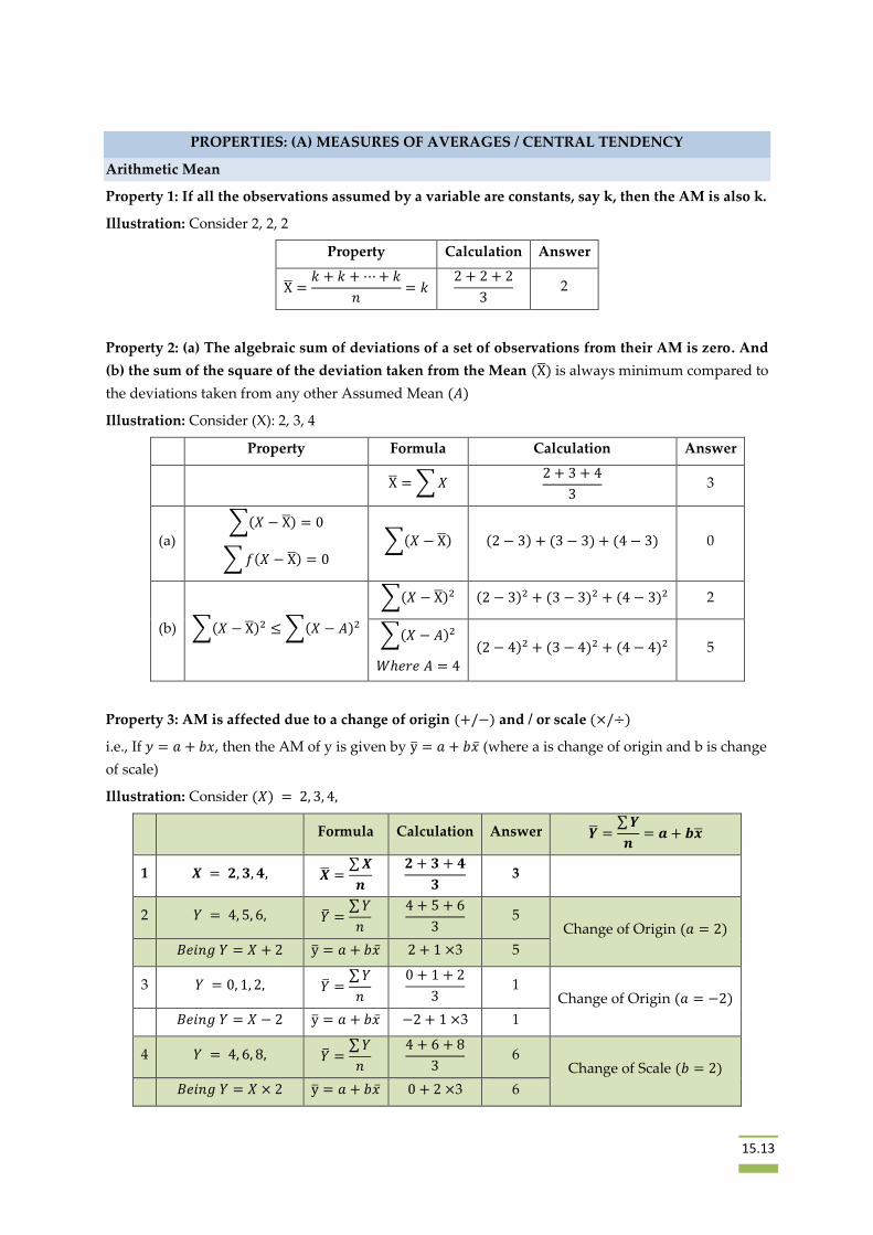
PROPERTIES: (A) MEASURES OF AVERAGES / CENTRAL TENDENCY
Arithmetic Mean
Property 1: If all the observations assumed by a variable are constants, say k, then the AM is also k.
Illustration: Consider 2, 2, 2
Property Calculation Answer
X̅ =𝑘 + 𝑘 + ⋯ + 𝑘
𝑛= 𝑘
2 + 2 + 2
3 2
Property 2: (a) The algebraic sum of deviations of a set of observations from their AM is zero. And
(b) the sum of the square of the deviation taken from the Mean (X̅) is always minimum compared to
the deviations taken from any other Assumed Mean (𝐴)
Illustration: Consider (X): 2, 3, 4
Property Formula Calculation Answer
X̅ = ∑ 𝑋 2 + 3 + 4
3 3
(a) ∑(𝑋 − X̅) = 0
∑ 𝑓(𝑋 − X̅) = 0 ∑(𝑋 − X̅) (2 − 3) + (3 − 3) + (4 − 3) 0
(b) ∑(𝑋 − X̅)2 ≤ ∑(𝑋 − 𝐴)2
∑(𝑋 − X̅)2 (2 − 3)2 + (3 − 3)2 + (4 − 3)2 2
∑(𝑋 − 𝐴)2
𝑊ℎ𝑒𝑟𝑒 𝐴 = 4
(2 − 4)2 + (3 − 4)2 + (4 − 4)2 5
Property 3: AM is affected due to a change of origin (+/−) and / or scale (×/÷)
i.e., If 𝑦 = 𝑎 + 𝑏𝑥, then the AM of y is given by y̅ = 𝑎 + 𝑏�̅� (where a is change of origin and b is change
of scale)
Illustration: Consider (𝑋) = 2, 3, 4,
Formula Calculation Answer �̅� =∑ 𝒀
𝒏= 𝒂 + 𝒃𝒙
1 𝑿 = 𝟐, 𝟑, 𝟒, �̅� =∑ 𝑿
𝒏
𝟐 + 𝟑 + 𝟒
𝟑 3
2 𝑌 = 4, 5, 6, �̅� =∑ 𝑌
𝑛
4 + 5 + 6
3 5
Change of Origin (𝑎 = 2)
𝐵𝑒𝑖𝑛𝑔 𝑌 = 𝑋 + 2 y̅ = 𝑎 + 𝑏�̅� 2 + 1 ×3 5
3 𝑌 = 0, 1, 2, �̅� =∑ 𝑌
𝑛
0 + 1 + 2
3 1
Change of Origin (𝑎 = −2)
𝐵𝑒𝑖𝑛𝑔 𝑌 = 𝑋 − 2 y̅ = 𝑎 + 𝑏�̅� −2 + 1 ×3 1
4 𝑌 = 4, 6, 8, �̅� =∑ 𝑌
𝑛
4 + 6 + 8
3 6
Change of Scale (𝑏 = 2)
𝐵𝑒𝑖𝑛𝑔 𝑌 = 𝑋 × 2 y̅ = 𝑎 + 𝑏�̅� 0 + 2 ×3 6
15.14
5 𝑌 = 1, 1.5, 2, �̅� =∑ 𝑌
𝑛
1 + 1.5 + 2
3 1.5
Change of Scale (𝑏 =1
2)
𝐵𝑒𝑖𝑛𝑔 𝑌 = 𝑋 ×1
2 y̅ = 𝑎 + 𝑏�̅� 0 +
1
2×3 1.5
6 𝑌 = 7, 9, 11, �̅� =∑ 𝑌
𝑛
7 + 9 + 11
3 9 Change of Origin and
change of scale
(𝑎 = 3)&(𝑏 = 2) 𝐵𝑒𝑖𝑛𝑔 𝑌 = 3 + 2 × 𝑋 y̅ = 𝑎 + 𝑏�̅� 3 + 2 ×3 9
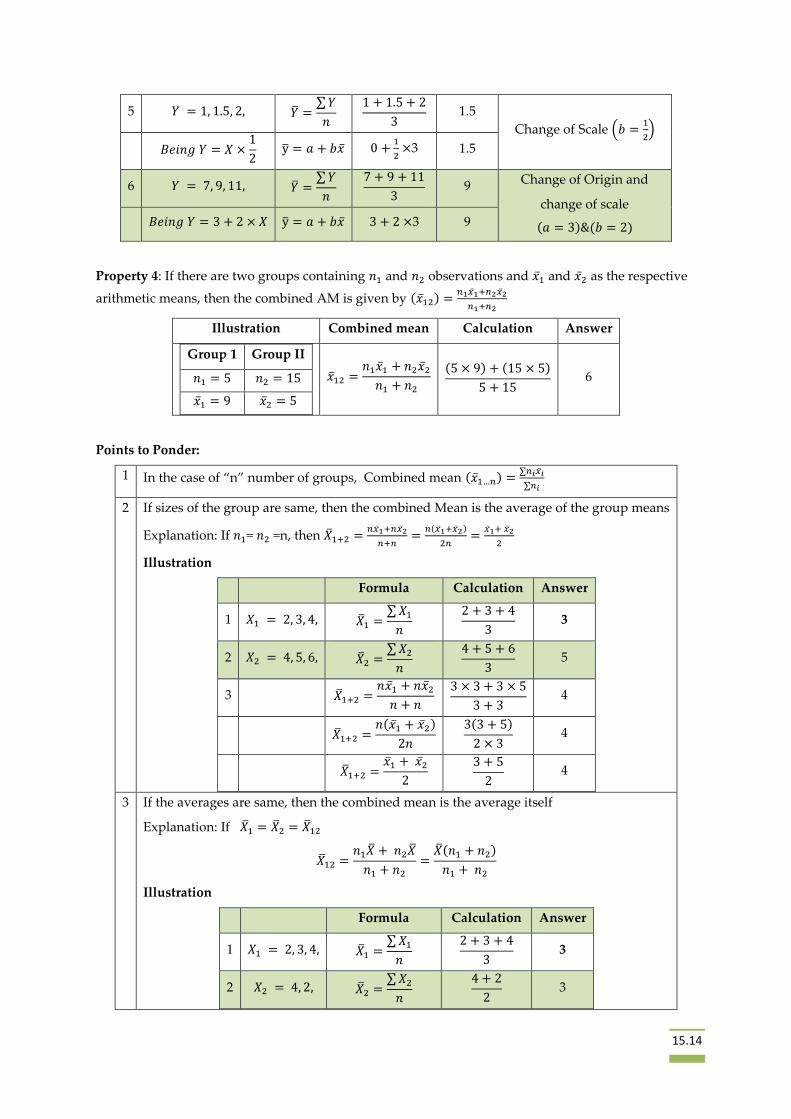
Property 4: If there are two groups containing 𝑛1 and 𝑛2 observations and �̅�1 and �̅�2 as the respective
arithmetic means, then the combined AM is given by (�̅�12) =𝑛1�̅�̅1+𝑛2�̅�̅2
𝑛1+𝑛2
Illustration Combined mean Calculation Answer
Group 1 Group II
𝑛1 = 5 𝑛2 = 15
�̅�1 = 9 �̅�2 = 5
�̅�12 =𝑛1�̅�1 + 𝑛2�̅�2
𝑛1 + 𝑛2
(5 × 9) + (15 × 5)
5 + 15 6
Points to Ponder:
1 In the case of “n” number of groups, Combined mean (�̅�1…𝑛) =∑𝑛𝑖�̅�̅𝑖
∑𝑛𝑖
2 If sizes of the group are same, then the combined Mean is the average of the group means
Explanation: If 𝑛1= 𝑛2 =n, then �̅�1+2 =𝑛�̅�̅1+𝑛�̅�̅2
𝑛+𝑛=
𝑛(�̅�̅1+�̅�̅2)
2𝑛=
�̅�̅1+ �̅�̅2
2
Illustration
Formula Calculation Answer
1 𝑋1 = 2, 3, 4, �̅�1 =∑ 𝑋1
𝑛
2 + 3 + 4
3 3
2 𝑋2 = 4, 5, 6, �̅�2 =∑ 𝑋2
𝑛
4 + 5 + 6
3 5
3 �̅�1+2 =𝑛�̅�1 + 𝑛�̅�2
𝑛 + 𝑛
3 × 3 + 3 × 5
3 + 3 4
�̅�1+2 =𝑛(�̅�1 + �̅�2)
2𝑛
3(3 + 5)
2 × 3 4
�̅�1+2 =�̅�1 + �̅�2
2
3 + 5
2 4
3 If the averages are same, then the combined mean is the average itself
Explanation: If �̅�1 = �̅�2 = �̅�12
�̅�12 =𝑛1�̅� + 𝑛2�̅�
𝑛1 + 𝑛2
=�̅�(𝑛1 + 𝑛2)
𝑛1 + 𝑛2
Illustration
Formula Calculation Answer
1 𝑋1 = 2, 3, 4, �̅�1 =∑ 𝑋1
𝑛
2 + 3 + 4
3 3
2 𝑋2 = 4, 2, �̅�2 =∑ 𝑋2
𝑛
4 + 2
2 3
15.15
3 �̅�1+2 =𝑛�̅�1 + 𝑛�̅�2
𝑛 + 𝑛
3 × 3 + 2 × 3
3 + 2 3
�̅�(𝑛1 + 𝑛2)
𝑛1 + 𝑛2
3(3 + 2)
2 + 3 3
�̅�1+2 = �̅�1 = �̅�2 3
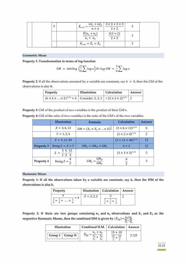
Geometric Mean
Property 1: Transformation in terms of log function
𝐺𝑀 = 𝐴𝑛𝑡𝑖𝑙𝑜𝑔 (1
𝑛∑ 𝑙𝑜𝑔 𝑥) 𝑂𝑟 𝑙𝑜𝑔 𝐺𝑀 =
1
𝑛∑ 𝑙𝑜𝑔 𝑥
Property 2: If all the observations assumed by a variable are constants, say 𝑘 > 0, then the GM of the
observations is also K.
Property Illustration Calculation Answer
(𝑘 × 𝑘 × … .× 𝑘)1 𝑛⁄ = 𝑘 Consider: 2, 2, 2 = (2 × 2 × 2)1 3⁄ 2
Property 3: GM of the product of two variables is the product of their GM‘s.
Property 4: GM of the ratio of two variables is the ratio of the GM’s of the two variables.
Illustration Formula Calculation Answer
𝑋 = 3, 6, 12 GM = (𝑋1 × 𝑋2 × … × 𝑋)1
𝑛 (3 × 6 × 12)1 3⁄ 6
𝑌 = 1, 2, 4 (1 × 2 × 4)1 3⁄ 2
𝑍 = 3, 12, 48 (3 × 12 × 48)1 3⁄ 12
Property 3 Being 𝑍 = 𝑋 × 𝑌 GM𝑍 = GM𝑋 × GM𝑌 6 × 2 12
𝑍 = 3
1,6
2,12
4 (3 × 3 × 3)1 3⁄ 3
Property 4 Being 𝑍 =𝑋
𝑌 𝐺𝑀𝑧 =
GM𝑋
GM𝑌
6
2 3
Harmonic Mean:
Property 1: If all the observations taken by a variable are constants, say k, then the HM of the
observations is also k.
Property Illustration Calculation Answer
𝑛1
𝑘+
1
𝑘+ … . +
1
𝑘
= 𝑘 𝑋 = 2, 2, 2 31
2+
1
2+
1
2
2
Property 2: If there are two groups containing 𝒏𝟏 and 𝒏𝟐 observations and 𝑿𝟏 and 𝑿𝟐 as the
respective Harmonic Means, then the combined HM is given by (�̅�𝟏𝟐) = 𝒏𝟏+𝒏𝟐𝒏𝟏�̅�𝟏
+ 𝒏𝟐�̅�𝟐
Illustration Combined H.M. Calculation Answer
Group 1 Group II �̅�𝟏𝟐 =𝑛1 + 𝑛2𝑛1
�̅�̅1+
𝑛2
�̅�̅2
15 + 1015
3+
10
2
3.125
15.16
𝑛1 = 15 𝑛2 = 10
�̅�1 = 3 �̅�2 = 2
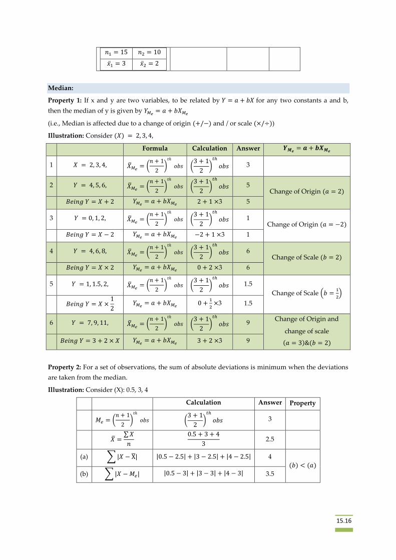
Median:
Property 1: If x and y are two variables, to be related by 𝑌 = 𝑎 + 𝑏𝑋 for any two constants a and b,
then the median of y is given by 𝑌𝑀𝑒= 𝑎 + 𝑏𝑋𝑀𝑒
(i.e., Median is affected due to a change of origin (+/−) and / or scale (×/÷))
Illustration: Consider (𝑋) = 2, 3, 4,
Formula Calculation Answer 𝒀𝑴𝒆= 𝒂 + 𝒃𝑿𝑴𝒆
1 𝑋 = 2, 3, 4, �̅�𝑀𝑒= (
𝑛 + 1
2)
𝑡ℎ
𝑜𝑏𝑠 (3 + 1
2)
𝑡ℎ
𝑜𝑏𝑠 3
2 𝑌 = 4, 5, 6, �̅�𝑀𝑒= (
𝑛 + 1
2)
𝑡ℎ
𝑜𝑏𝑠 (3 + 1
2)
𝑡ℎ
𝑜𝑏𝑠 5 Change of Origin (𝑎 = 2)
𝐵𝑒𝑖𝑛𝑔 𝑌 = 𝑋 + 2 𝑌𝑀𝑒= 𝑎 + 𝑏𝑋𝑀𝑒
2 + 1 ×3 5
3 𝑌 = 0, 1, 2, �̅�𝑀𝑒= (
𝑛 + 1
2)
𝑡ℎ
𝑜𝑏𝑠 (3 + 1
2)
𝑡ℎ
𝑜𝑏𝑠 1 Change of Origin (𝑎 = −2)
𝐵𝑒𝑖𝑛𝑔 𝑌 = 𝑋 − 2 𝑌𝑀𝑒= 𝑎 + 𝑏𝑋𝑀𝑒
−2 + 1 ×3 1
4 𝑌 = 4, 6, 8, �̅�𝑀𝑒= (
𝑛 + 1
2)
𝑡ℎ
𝑜𝑏𝑠 (3 + 1
2)
𝑡ℎ
𝑜𝑏𝑠 6 Change of Scale (𝑏 = 2)
𝐵𝑒𝑖𝑛𝑔 𝑌 = 𝑋 × 2 𝑌𝑀𝑒= 𝑎 + 𝑏𝑋𝑀𝑒
0 + 2 ×3 6
5 𝑌 = 1, 1.5, 2, �̅�𝑀𝑒= (
𝑛 + 1
2)
𝑡ℎ
𝑜𝑏𝑠 (3 + 1
2)
𝑡ℎ
𝑜𝑏𝑠 1.5
Change of Scale (𝑏 =1
2)
𝐵𝑒𝑖𝑛𝑔 𝑌 = 𝑋 ×1
2 𝑌𝑀𝑒
= 𝑎 + 𝑏𝑋𝑀𝑒 0 +
1
2×3 1.5
6 𝑌 = 7, 9, 11, �̅�𝑀𝑒= (
𝑛 + 1
2)
𝑡ℎ
𝑜𝑏𝑠 (3 + 1
2)
𝑡ℎ
𝑜𝑏𝑠 9 Change of Origin and
change of scale
(𝑎 = 3)&(𝑏 = 2) 𝐵𝑒𝑖𝑛𝑔 𝑌 = 3 + 2 × 𝑋 𝑌𝑀𝑒= 𝑎 + 𝑏𝑋𝑀𝑒
3 + 2 ×3 9
Property 2: For a set of observations, the sum of absolute deviations is minimum when the deviations
are taken from the median.
Illustration: Consider (X): 0.5, 3, 4
Calculation Answer Property
𝑀𝑒 = (𝑛 + 1
2)
𝑡ℎ
𝑜𝑏𝑠 (3 + 1
2)
𝑡ℎ
𝑜𝑏𝑠 3
�̅� =∑ 𝑋
𝑛
0.5 + 3 + 4
3 2.5
(a) ∑ |𝑋 − X̅| |0.5 − 2.5| + |3 − 2.5| + |4 − 2.5| 4
(𝑏) < (𝑎)
(b) ∑ |𝑋 − 𝑀𝑒| |0.5 − 3| + |3 − 3| + |4 − 3| 3.5
15.17
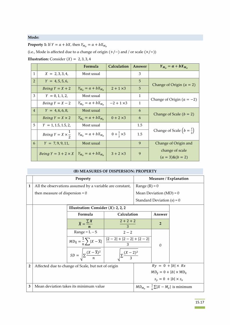
Mode:
Property 1: If 𝑌 = 𝑎 + 𝑏𝑋, then 𝑌𝑀𝑜= 𝑎 + 𝑏𝑋𝑀𝑜
(i.e., Mode is affected due to a change of origin (+/−) and / or scale (×/÷))
Illustration: Consider (𝑋) = 2, 3, 3, 4
Formula Calculation Answer 𝒀𝑴𝒐= 𝒂 + 𝒃𝑿𝑴𝒐
1 𝑋 = 2, 3, 3, 4, Most usual 3
2 𝑌 = 4, 5, 5, 6, 5 Change of Origin (𝑎 = 2)
𝐵𝑒𝑖𝑛𝑔 𝑌 = 𝑋 + 2 𝑌𝑀𝑜= 𝑎 + 𝑏𝑋𝑀𝑜
2 + 1 ×3 5
3 𝑌 = 0, 1, 1, 2, Most usual 1 Change of Origin (𝑎 = −2)
𝐵𝑒𝑖𝑛𝑔 𝑌 = 𝑋 − 2 𝑌𝑀𝑜= 𝑎 + 𝑏𝑋𝑀𝑜
−2 + 1 ×3 1
4 𝑌 = 4, 6, 6, 8, Most usual 6 Change of Scale (𝑏 = 2)
𝐵𝑒𝑖𝑛𝑔 𝑌 = 𝑋 × 2 𝑌𝑀𝑒= 𝑎 + 𝑏𝑋𝑀𝑒
0 + 2 ×3 6
5 𝑌 = 1, 1.5, 1.5, 2, Most usual 1.5
Change of Scale (𝑏 =1
2)
𝐵𝑒𝑖𝑛𝑔 𝑌 = 𝑋 ×1
2 𝑌𝑀𝑜
= 𝑎 + 𝑏𝑋𝑀𝑜 0 +
1
2×3 1.5
6 𝑌 = 7, 9, 9, 11, Most usual 9 Change of Origin and
change of scale
(𝑎 = 3)&(𝑏 = 2) 𝐵𝑒𝑖𝑛𝑔 𝑌 = 3 + 2 × 𝑋 𝑌𝑀𝑜
= 𝑎 + 𝑏𝑋𝑀𝑜 3 + 2 ×3 9
(B) MEASURES OF DISPERSION: PROPERTY
Property Measure / Explanation
1 All the observations assumed by a variable are constant,
then measure of dispersion = 0
Range (R) = 0
Mean Deviation (MD) = 0
Standard Deviation (s) = 0
Illustration: Consider (𝑿): 2, 2, 2
Formula Calculation Answer
�̅� =∑ 𝑿
𝒏
2 + 2 + 2
3 2
Range = L – S 2 − 2
0 𝑀𝐷X̅ =
1
𝑛∑|𝑋 − X̅|
|2 − 2| + |2 − 2| + |2 − 2|
3
𝑆𝐷 = √∑(𝑋 − X̅)2
𝑛 √∑
(𝑋 − 2)2
3
2 Affected due to change of Scale, but not of origin 𝑅𝑦 = 0 + |𝑏| × 𝑅𝑥
𝑀𝐷y̅ = 0 + |𝑏| × MDx̅
𝑠𝑦 = 0 + |𝑏| × 𝑠𝑥̅
3 Mean deviation takes its minimum value 𝑀𝐷𝑀𝑒=
1
𝑛∑|𝑋 − 𝑀𝑒| is minimum
15.18
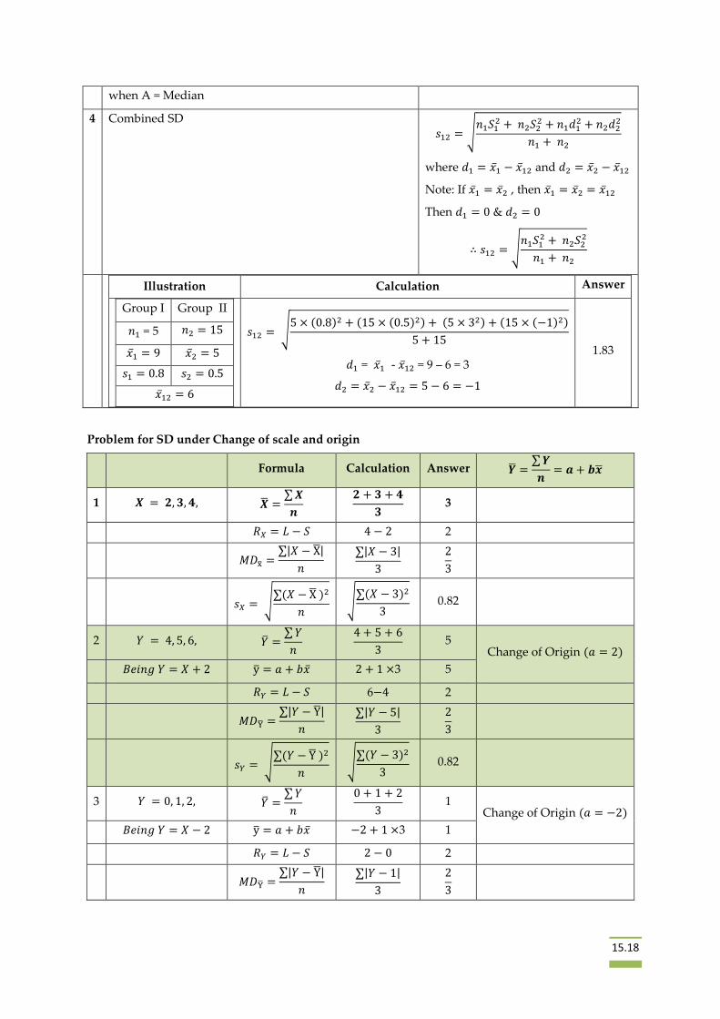
when A = Median
4 Combined SD 𝑠12 = √
𝑛1𝑆12 + 𝑛2𝑆2
2 + 𝑛1𝑑12 + 𝑛2𝑑2
2
𝑛1 + 𝑛2
where 𝑑1 = �̅�1 − �̅�12 and 𝑑2 = �̅�2 − �̅�12
Note: If �̅�1 = �̅�2 , then �̅�1 = �̅�2 = �̅�12
Then 𝑑1 = 0 & 𝑑2 = 0
∴ 𝑠12 = √𝑛1𝑆1
2 + 𝑛2𝑆22
𝑛1 + 𝑛2
Illustration Calculation Answer
Group I Group II
𝑛1 = 5 𝑛2 = 15
�̅�1 = 9 �̅�2 = 5
𝑠1 = 0.8 𝑠2 = 0.5
�̅�12 = 6
𝑠12 = √5 × (0.8)2 + (15 × (0.5)2) + (5 × 32) + (15 × (−1)2)
5 + 15
𝑑1 = �̅�1 - �̅�12 = 9 – 6 = 3
𝑑2 = �̅�2 − �̅�12 = 5 − 6 = −1
1.83
Problem for SD under Change of scale and origin
Formula Calculation Answer �̅� =∑ 𝒀
𝒏= 𝒂 + 𝒃𝒙
1 𝑿 = 𝟐, 𝟑, 𝟒, �̅� =∑ 𝑿
𝒏
𝟐 + 𝟑 + 𝟒
𝟑 3
𝑅𝑋 = 𝐿 − 𝑆 4 − 2 2
𝑀𝐷x̅ =∑|𝑋 − X̅|
𝑛
∑|𝑋 − 3|
3
2
3
𝑠𝑋 = √∑(𝑋 − X̅ )2
𝑛 √
∑(𝑋 − 3)2
3 0.82
2 𝑌 = 4, 5, 6, �̅� =∑ 𝑌
𝑛
4 + 5 + 6
3 5
Change of Origin (𝑎 = 2)
𝐵𝑒𝑖𝑛𝑔 𝑌 = 𝑋 + 2 y̅ = 𝑎 + 𝑏�̅� 2 + 1 ×3 5
𝑅𝑌 = 𝐿 − 𝑆 6−4 2
𝑀𝐷Y̅ =∑|𝑌 − Y̅|
𝑛
∑|𝑌 − 5|
3
2
3
𝑠𝑌 = √∑(𝑌 − Y̅ )2
𝑛 √
∑(𝑌 − 3)2
3 0.82
3 𝑌 = 0, 1, 2, �̅� =∑ 𝑌
𝑛
0 + 1 + 2
3 1
Change of Origin (𝑎 = −2)
𝐵𝑒𝑖𝑛𝑔 𝑌 = 𝑋 − 2 y̅ = 𝑎 + 𝑏�̅� −2 + 1 ×3 1
𝑅𝑌 = 𝐿 − 𝑆 2 − 0 2
𝑀𝐷Y̅ =∑|𝑌 − Y̅|
𝑛
∑|𝑌 − 1|
3
2
3
15.19
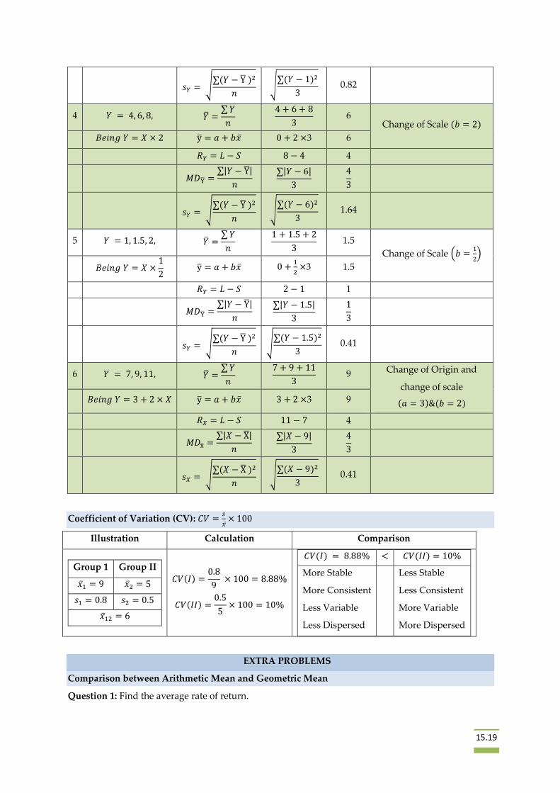
𝑠𝑌 = √∑(𝑌 − Y̅ )2
𝑛 √
∑(𝑌 − 1)2
3 0.82
4 𝑌 = 4, 6, 8, �̅� =∑ 𝑌
𝑛
4 + 6 + 8
3 6
Change of Scale (𝑏 = 2)
𝐵𝑒𝑖𝑛𝑔 𝑌 = 𝑋 × 2 y̅ = 𝑎 + 𝑏�̅� 0 + 2 ×3 6
𝑅𝑌 = 𝐿 − 𝑆 8 − 4 4
𝑀𝐷Y̅ =∑|𝑌 − Y̅|
𝑛
∑|𝑌 − 6|
3
4
3
𝑠𝑌 = √∑(𝑌 − Y̅ )2
𝑛 √
∑(𝑌 − 6)2
3 1.64
5 𝑌 = 1, 1.5, 2, �̅� =∑ 𝑌
𝑛
1 + 1.5 + 2
3 1.5
Change of Scale (𝑏 =1
2)
𝐵𝑒𝑖𝑛𝑔 𝑌 = 𝑋 ×1
2 y̅ = 𝑎 + 𝑏�̅� 0 +
1
2×3 1.5
𝑅𝑌 = 𝐿 − 𝑆 2 − 1 1
𝑀𝐷Y̅ =∑|𝑌 − Y̅|
𝑛
∑|𝑌 − 1.5|
3
1
3
𝑠𝑌 = √∑(𝑌 − Y̅ )2
𝑛 √
∑(𝑌 − 1.5)2
3 0.41
6 𝑌 = 7, 9, 11, �̅� =∑ 𝑌
𝑛
7 + 9 + 11
3 9 Change of Origin and
change of scale
(𝑎 = 3)&(𝑏 = 2) 𝐵𝑒𝑖𝑛𝑔 𝑌 = 3 + 2 × 𝑋 y̅ = 𝑎 + 𝑏�̅� 3 + 2 ×3 9
𝑅𝑋 = 𝐿 − 𝑆 11 − 7 4
𝑀𝐷x̅ =∑|𝑋 − X̅|
𝑛
∑|𝑋 − 9|
3
4
3
𝑠𝑋 = √∑(𝑋 − X̅ )2
𝑛 √
∑(𝑋 − 9)2
3 0.41
Coefficient of Variation (CV): 𝐶𝑉 =𝑠
�̅�̅× 100
Illustration Calculation Comparison
Group 1 Group II
�̅�1 = 9 �̅�2 = 5
𝑠1 = 0.8 𝑠2 = 0.5
�̅�12 = 6
𝐶𝑉(𝐼) =0.8
9 × 100 = 8.88%
𝐶𝑉(𝐼𝐼) =0.5
5× 100 = 10%
𝐶𝑉(𝐼) = 8.88% < 𝐶𝑉(𝐼𝐼) = 10%
More Stable
More Consistent
Less Variable
Less Dispersed
Less Stable
Less Consistent
More Variable
More Dispersed
EXTRA PROBLEMS
Comparison between Arithmetic Mean and Geometric Mean
Question 1: Find the average rate of return.
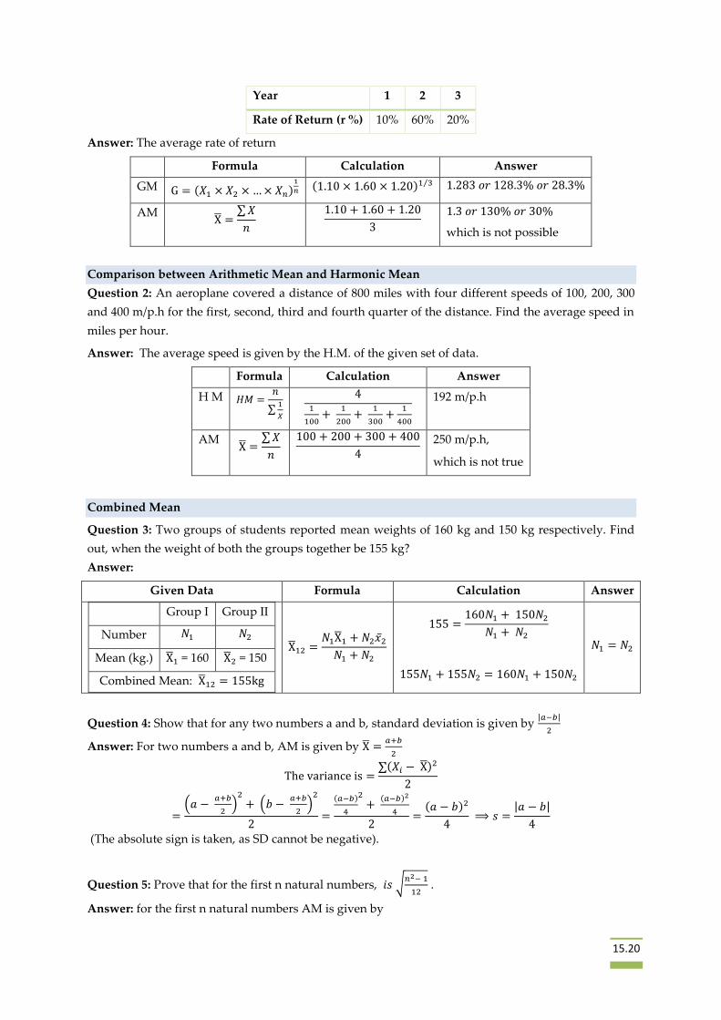
15.20
Year 1 2 3
Rate of Return (r %) 10% 60% 20%
Answer: The average rate of return
Formula Calculation Answer
GM G = (𝑋1 × 𝑋2 × … × 𝑋𝑛)1
𝑛 (1.10 × 1.60 × 1.20)1 3⁄ 1.283 𝑜𝑟 128.3% 𝑜𝑟 28.3%
AM X̅ =
∑ 𝑋
𝑛
1.10 + 1.60 + 1.20
3
1.3 𝑜𝑟 130% 𝑜𝑟 30%
which is not possible
Comparison between Arithmetic Mean and Harmonic Mean
Question 2: An aeroplane covered a distance of 800 miles with four different speeds of 100, 200, 300
and 400 m/p.h for the first, second, third and fourth quarter of the distance. Find the average speed in
miles per hour.
Answer: The average speed is given by the H.M. of the given set of data.
Formula Calculation Answer
H M 𝐻𝑀 =𝑛
∑1
𝑋
41
100+
1
200+
1
300+
1
400
192 m/p.h
AM X̅ =
∑ 𝑋
𝑛
100 + 200 + 300 + 400
4
250 m/p.h,
which is not true
Combined Mean
Question 3: Two groups of students reported mean weights of 160 kg and 150 kg respectively. Find
out, when the weight of both the groups together be 155 kg?
Answer:
Given Data Formula Calculation Answer
Group I Group II
Number 𝑁1 𝑁2
Mean (kg.) X̅1 = 160 X̅2 = 150
Combined Mean: X̅12 = 155kg
X̅12 =𝑁1X̅1 + 𝑁2�̅�2
𝑁1 + 𝑁2
155 =160𝑁1 + 150𝑁2
𝑁1 + 𝑁2
155𝑁1 + 155𝑁2 = 160𝑁1 + 150𝑁2
𝑁1 = 𝑁2
Question 4: Show that for any two numbers a and b, standard deviation is given by |𝑎−𝑏|
2
Answer: For two numbers a and b, AM is given by X̅ =𝑎+𝑏
2
The variance is =∑(𝑋𝑖 − X̅)2
2
=(𝑎 −
𝑎+𝑏
2)
2
+ (𝑏 − 𝑎+𝑏
2)
2
2=
(𝑎−𝑏)
4
2
+ (𝑎−𝑏)2
4
2=
(𝑎 − 𝑏)2
4 ⟹ 𝑠 =
|𝑎 − 𝑏|
4
(The absolute sign is taken, as SD cannot be negative).
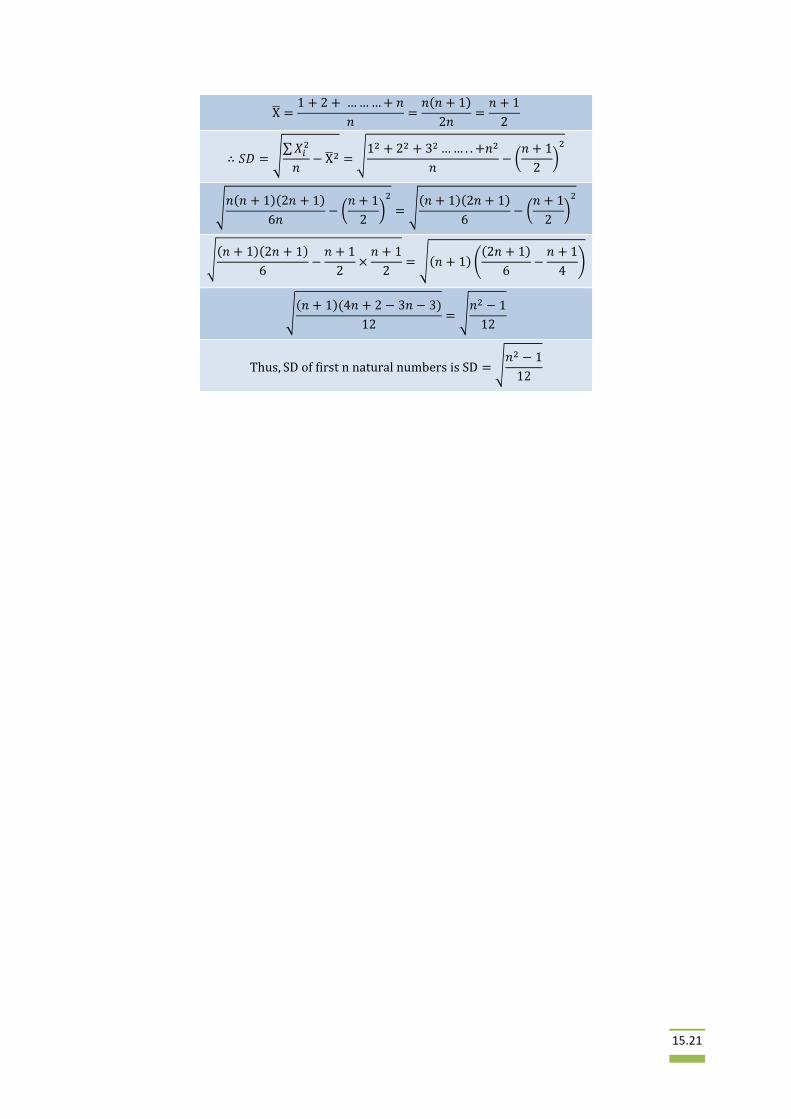
Question 5: Prove that for the first n natural numbers, 𝑖𝑠 √𝑛2− 1
12 .
Answer: for the first n natural numbers AM is given by
15.21
X̅ =1 + 2 + … … … + 𝑛
𝑛=
𝑛(𝑛 + 1)
2𝑛=
𝑛 + 1
2
∴ 𝑆𝐷 = √∑ 𝑋𝑖
2
𝑛− X̅2 = √
12 + 22 + 32 … … . . +𝑛2
𝑛− (
𝑛 + 1
2)
2
√𝑛(𝑛 + 1)(2𝑛 + 1)
6𝑛− (
𝑛 + 1
2)
2
= √(𝑛 + 1)(2𝑛 + 1)
6− (
𝑛 + 1
2)
2
√(𝑛 + 1)(2𝑛 + 1)
6−
𝑛 + 1
2×
𝑛 + 1
2= √(𝑛 + 1) (
(2𝑛 + 1)
6−
𝑛 + 1
4)
√(𝑛 + 1)(4𝑛 + 2 − 3𝑛 − 3)
12= √
𝑛2 − 1
12
Thus, SD of first n natural numbers is SD = √𝑛2 − 1
12

15.22
COMPARISON BETWEEN MEASURES OF CENTRAL TENDENCY N
o
Mea
sure
s
Ari
thm
etic
Mea
n
Geo
met
ric
Mea
n
Har
mo
nic
Mea
n
Med
ian
Mo
de
Ran
ge
Qu
arti
le
Dev
iati
on
Mea
n
Dev
iati
on
Sta
nd
ard
Dev
iati
on
1 Well defined Yes Yes Yes Yes
No (when the
number of
observations is
small, then use
Empirical
Relationship)
Yes Yes A may be
X̅, 𝑀𝑒, 𝑀𝑜 Yes
2 Easy to calculate &
simple to understand Yes No No Yes
Location Method,
but not Grouping
method
Yes Yes Yes No
3 Based on all the
items Yes
Yes (but able
to find only
for Positive
Values)
Yes
(ONLY
positive
values
and no
“0”)
No No No No Yes Yes
4
capable of further
mathematical
treatment
Yes
Yes (Useful
for
calculation of
Index
Numbers)
Yes
Yes (but only in
Mean Deviation,
no combined
Median)
No
No (But in case
of Quality
control and stock
market
fluctuations)
No
No (Useful for
Economists and
Businessmen and
in public reports)
Yes
5 Good basis for
comparison Yes Not much Yes
6 Necessary for
arrange of data No No No Yes No ------Not on Discussion-----
7 Affected by extreme
values Yes
Yes (Not
much
compared to
Yes No No Yes No Less than SD Yes

15.23
AM)
8
Not Precise – Mis-
leading impressions
(E.g. Average
number of persons is
1.5 which is not
possible)
No
No No
Yes (except
when Median
lies in between
two values)
Yes (except on
continuous series) ------Not on Discussion-----
9 Location (Inspection)
Method No No No
Yes (on
arrangement) Yes ------Not on Discussion-----
10 Graphical Method Yes (using Ogive
Curves) ------Not on Discussion-----
11
Calculated in the
case of open end
class intervals
No No No Yes Yes No Yes Based on “A” No
12
Affected by
sampling
fluctuations
No
(least) No No Yes Yes Yes Yes Yes
Less
affected
13
Affected by Change
of origin Yes Yes Yes Yes Yes No No No No
Affected by Change
of Scale Yes Yes Yes Yes Yes Yes Yes Yes Yes
15.24
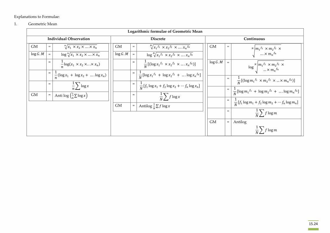
Explanations to Formulae:
1. Geometric Mean
Logarithmic formulae of Geometric Mean
Individual Observation Discrete Continuous
GM = √𝑥1 × 𝑥2 × … .× 𝑥𝑛𝑛
log 𝐺. 𝑀 = log √𝑥1 × 𝑥2 × … .× 𝑥𝑛𝑛
= 1
𝑛log(𝑥1 × 𝑥2 ×. . .× 𝑥𝑛)
= 1
𝑛(log 𝑥1 + log 𝑥2 + … . log 𝑥𝑛)
= 1
𝑛∑ log 𝑥
GM = Anti log (1
𝑛∑ log 𝑥)
GM = √𝑥1𝑓1 × 𝑥2
𝑓2 × … . 𝑥𝑛𝑓𝑛
𝑁
log 𝐺. 𝑀 = log √𝑥1𝑓1 × 𝑥2
𝑓2 × … . 𝑥𝑛𝑓𝑛
𝑁
= 1
𝑁[(log 𝑥1
𝑓1 × 𝑥2𝑓2 × … . 𝑥𝑛
𝑓𝑛)]
= 1
𝑁[log 𝑥1
𝑓1 + log 𝑥2𝑓2 + … . log 𝑥𝑛
𝑓𝑛]
= 1
𝑁[𝑓1 log 𝑥1 + 𝑓2 log 𝑥2 + ⋯ 𝑓𝑛 log 𝑥𝑛]
= 1
𝑁∑ 𝑓 log 𝑥
GM = Antilog 1
𝑁∑ 𝑓 log 𝑥
GM = √
𝑚1𝑓1 × 𝑚2
𝑓2 ×
… .× 𝑚𝑛𝑓𝑛
𝑁
log 𝐺. 𝑀 = log √
𝑚1𝑓1 × 𝑚2
𝑓2 ×
… × 𝑚𝑛𝑓𝑛
𝑁
= 1
𝑁[(log 𝑚1
𝑓1 × 𝑚2𝑓2 × … × 𝑚𝑛
𝑓𝑛)]
= 1
𝑁[log 𝑚1
𝑓1 + log 𝑚2𝑓2 + … . log 𝑚𝑛
𝑓𝑛]
= 1
𝑁[𝑓1 log 𝑚1 + 𝑓2 log 𝑚2 + ⋯ 𝑓𝑛 log 𝑚𝑛]
= 1
𝑁∑ 𝑓 log 𝑚
GM = Antilog
1
𝑁∑ 𝑓 log 𝑚
15.25
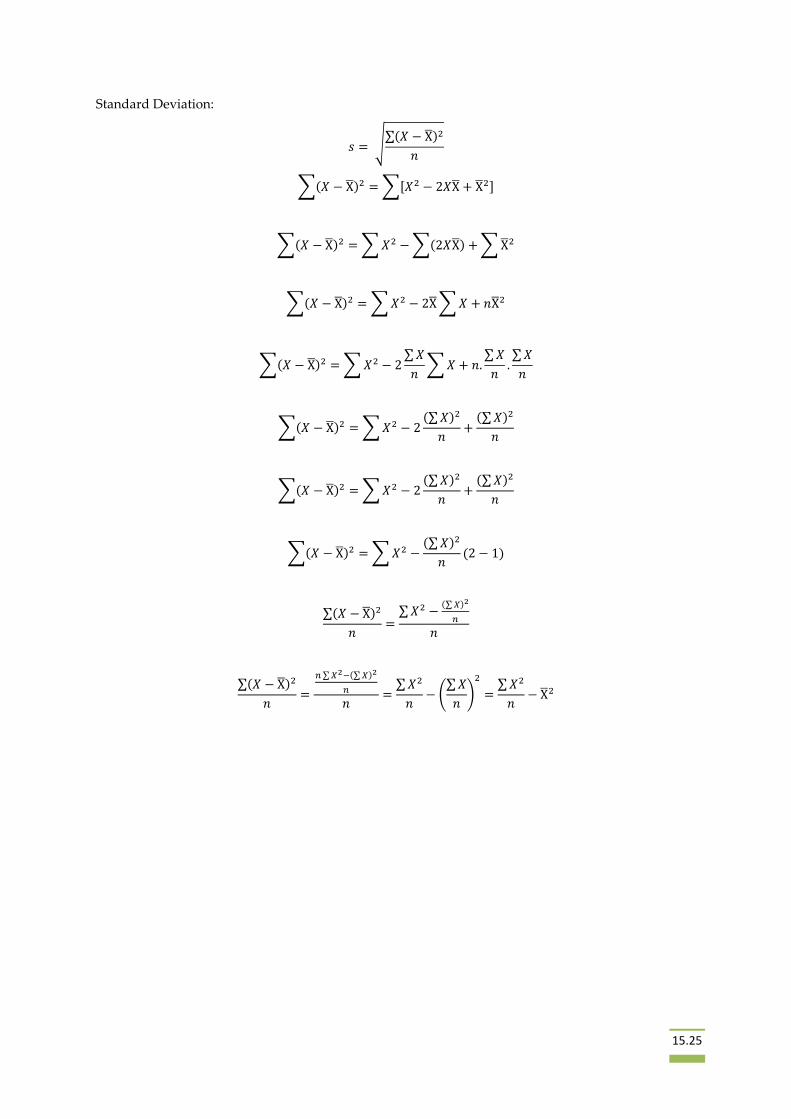
Standard Deviation:
𝑠 = √∑(𝑋 − X̅)2
𝑛
∑(𝑋 − X̅)2 = ∑[𝑋2 − 2𝑋X̅ + X̅2]
∑(𝑋 − X̅)2 = ∑ 𝑋2 − ∑(2𝑋X̅) + ∑ X̅2
∑(𝑋 − X̅)2 = ∑ 𝑋2 − 2X̅ ∑ 𝑋 + 𝑛X̅2
∑(𝑋 − X̅)2 = ∑ 𝑋2 − 2∑ 𝑋
𝑛∑ 𝑋 + 𝑛.
∑ 𝑋
𝑛.∑ 𝑋
𝑛
∑(𝑋 − X̅)2 = ∑ 𝑋2 − 2(∑ 𝑋)2
𝑛+
(∑ 𝑋)2
𝑛
∑(𝑋 − X̅)2 = ∑ 𝑋2 − 2(∑ 𝑋)2
𝑛+
(∑ 𝑋)2
𝑛
∑(𝑋 − X̅)2 = ∑ 𝑋2 −(∑ 𝑋)2
𝑛(2 − 1)
∑(𝑋 − X̅)2
𝑛=
∑ 𝑋2 −(∑ 𝑋)2
𝑛
𝑛
∑(𝑋 − X̅)2
𝑛=
𝑛 ∑ 𝑋2−(∑ 𝑋)2
𝑛
𝑛=
∑ 𝑋2
𝑛− (
∑ 𝑋
𝑛)
2
=∑ 𝑋2
𝑛− X̅2
15.26
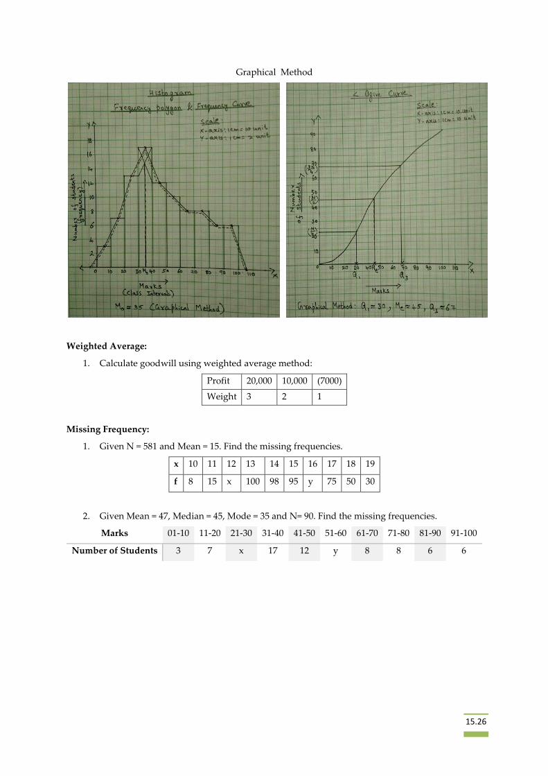
Graphical Method
Weighted Average:
1. Calculate goodwill using weighted average method:
Profit 20,000 10,000 (7000)
Weight 3 2 1
Missing Frequency:
1. Given N = 581 and Mean = 15. Find the missing frequencies.
x 10 11 12 13 14 15 16 17 18 19
f 8 15 x 100 98 95 y 75 50 30
2. Given Mean = 47, Median = 45, Mode = 35 and N= 90. Find the missing frequencies.
Marks 01-10 11-20 21-30 31-40 41-50 51-60 61-70 71-80 81-90 91-100
Number of Students 3 7 x 17 12 y 8 8 6 6