Statistics of extremes and estimation of extreme rainfall

2. Empirical investigation of long rainfall records

Demetris Koutsoyiannis

Department of Water Resources, Faculty of Civil Engineering, National Technical University of

Athens, Heroon Polytechneiou 5, GR-157 80 Zographou, Greece (dk@itia.ntua.gr)

Abstract In the first part of this study, theoretical analyses showed that the Gumbel

distribution is quite unlikely to apply to hydrological extremes and that the extreme value

distribution of type II (EV2) is a more consistent choice. Based on these theoretical analyses,

an extensive empirical investigation is performed using a collection of 169 of the longest

available rainfall records worldwide, each having 100-154 years of data. This verifies the

theoretical results. In addition, it shows that the shape parameter of the EV2 distribution is

constant for all examined geographical zones (Europe and North America), with value κ =

0.15. This simplifies the fitting and the general mathematical handling of the distribution,

which become as simple as those of the Gumbel distribution.

Keywords design rainfall; extreme rainfall; generalized extreme value distribution; Gumbel

distribution; hydrological design; hydrological extremes; probable maximum precipitation;

risk.

Statistique de valeurs extrêmes et estimation de précipitations extrêmes

2. Recherche empirique sur de longues séries de précipitations

Résumé Dans la première partie de cette étude, des analyses théoriques ont prouvé que la

distribution de Gumbel est peu susceptible de s'appliquer aux valeurs extrêmes de variables

hydrologiques et que la distribution de valeurs extrêmes du type II (EV2) est un choix plus

cohérent. Se basant sur ces analyses théoriques, une recherche empirique étendue est

effectuée en utilisant une collection de 169 parmi les séries de précipitations les plus longues

qui sont disponibles dans le monde entier, chacun comportant 100-154 ans de données. Ceci

2

vérifie les résultats théoriques. En outre, on montre que le paramètre de forme de la

distribution EV2 est constant pour toutes les zones géographiques examinées (l'Europe et

l'Amérique du Nord), avec sa valeur égale à 0.15. Ceci simplifie l'ajustement et la

manipulation mathématique générale de la distribution, qui deviennent aussi simples que ceux

de la distribution de Gumbel.

Mots-clés Précipitations de projet; précipitations extrêmes; distribution généralisée de valeurs

extrêmes; Distribution de Gumbel; conception hydrologique; valeurs extrêmes en hydrologie;

précipitation maximum probable; risque.

1. Introduction

According to the statistical theory of extremes, the distribution function H(x) of the maximum

of a number n of identically distributed random variables with distribution F(x), if n is large

enough (theoretically infinite), takes the asymptotic form, known as the Generalized Extreme

Value (GEV) distribution (Jenkinson, 1955, 1969),

H(x) = exp

–

1 + κ

x λ – ψ

–1 / κ

, κ x ≥ κ λ (ψ – 1 / κ) (1)

where ψ, λ > 0 and κ are location, scale and shape parameters, respectively. (Note that the sign

convention of κ in (1) is opposite to that most commonly used in hydrological texts and the

location parameter is dimensionless).

When κ = 0, the type I distribution of maxima (EV1 or Gumbel distribution),

H(x) = exp[–exp (–x/λ + ψ)] (2)

is obtained, which is unbounded from both below and above (–∞ < x < +∞). When κ > 0, H(x)

represents the extreme value distribution of maxima of type II (EV2), which is bounded from

below and unbounded from above (λ ψ – λ/κ ≤ x < +∞). A special case, the Fréchet

distribution, is obtained when the lower bound becomes zero (ψ = 1/κ), in which

Η(x) = exp

–

λ

κ x1/κ

, x ≥ 0 (3)

3

When κ < 0, H(x) represents the type III (EV3) distribution of maxima. This, however, is of

no practical interest in hydrology as it refers to random variables bounded from above (–∞ < x

≤ λ ψ – λ/κ).

There is a complete correspondence between the distribution of maxima H(x) and the tail

of F(x), which can be represented by the distribution of x conditional on being greater than a

certain threshold ξ, i.e., G(x) := F(x|x > ξ). For appropriate choice of ξ, it can be shown that

(see first part of the study)

G(x) = 1 –

1 + κ

x

λ – ψ –1 / κ

, x ≥ λ ψ (4)

which is the Pareto distribution. For κ > 0 this corresponds to the EV2 distribution whereas

for κ = 0 it takes the form

G(x) = 1 – exp (–x/λ + ψ), x ≥ λ ψ (5)

which is the exponential distribution and corresponds to the EV1 distribution. For the special

case ψ = 1/κ

G(x) = 1 –

λ

κ x1/κ

, x ≥ λ/κ (6)

The latter equation, is equivalentently written in the power law form x = (λ/κ) T κ, where T :=

1 / [1 – G(x)] is the return period. In the generalized Pareto case (4), the corresponding

relationship is x = (λ/κ) (T κ – 1 + κ ψ).

In hydrological applications, H(x) is fitted to annual maximum series of a hydrological

quantity such as rainfall depth of certain duration, whereas G(x) is fitted to series of values

over threshold (also known as partial duration series) of the same quantity. In the latter case,

the threshold is chosen so that the number of events (greater than the threshold) equals the

number of years of record.

The EV1 distribution has been the prevailing model for rainfall extremes despite the fact

that it results in the highest possible risk for engineering structures, i.e. it yields the smallest

possible design rainfall values in comparison to those of the EV2 for any value of the shape

parameter. The simplicity of the calculations of the EV1 distribution along with its

4

geometrical elucidation through a linear probability plot may have contributed to its

popularity in hydrologists and engineers. There is also a theoretical justification, as EV1 is the

asymptotic extreme value distribution for a wide range of parent distributions that are

common in hydrology.

However, the theoretical investigation of part 1 of this study shows that convergence of the

exact distribution of maxima to the asymptote EV1 may be extremely slow, thus making the

EV1 distribution an inappropriate approximation of the exact distribution of maxima. Besides,

the attraction of parent distributions to this asymptote relies on a stationarity assumption, i.e.

the assumption that parameters of the parent distribution are constant in time, which may not

be the case in hydrological processes. Slight relaxation of this assumption may result in the

EV2 rather than the EV1 asymptote.

Simulation experiments of part 1 of this study showed that small sizes of records, e.g. 20-

50 years, hide the EV2 distribution and display it as if it were EV1. This allowed the

conjecture that the broad use of the EV1 distribution worldwide may in fact be related to

small sample sizes rather than to the real behaviour of rainfall maxima, which should be better

described by the EV2 distribution. This conjecture is investigated thoroughly here based on

real-world long rainfall records.

2. Data

Some thousands of raingauge data sets from Europe and USA were examined in this study,

namely data from the United States Historical Climatology Network (USHCN), Land Surface

Observation Data of the UK ‘Met Office’, and data from the oldest stations of France, Italy

and Greece. Among these, a total of 169 stations were found to have at least 100 years of data

(not including the years with missing data) and were chosen for further analysis. Their

geographical locations are shown in Figure 1, classified in six geographical zones. Table 1

shows the general characteristics of raingauges of the different geographical zones and Table

2 gives the general characteristics of the top ten, in terms of record length, raingauges, which

are from all countries of this case study (USA, UK, France, Italy and Greece) and are located

in four of the six zones.

5

For all stations, all recorded data values through the station operation were available with

the exception of Athens, Greece, where only the annual maximum daily rainfall values were

available. From the continuous record of each station (except Athens), two series were

extracted, the series of annual maximum values of daily rainfall and the series of values over a

threshold chosen so that the number of values equals the number of years of the record. In

some of the records there were several missing values or values marked as incorrect, which

were deleted. Years with more than five missing daily values in two or more months were

excluded. In this way, 169 annual maximum series and 168 series of values over threshold

were constructed.

3. Initial exploration

As an initial step, the typical statistics and the L-statistics (based on probability-weighted

moments; Hosking 1990) were estimated for each annual maximum series of daily rainfall

depths. The ranges in each of the six geographical zones and the corresponding averages over

all stations of each zone are shown in Table 3. Potential relationships among these statistics

and their geographical variation were subsequently explored.

The sample mean (µ) and maximum values (xmax) over the observation period of each

annual maximum daily rainfall series are plotted in the log-log diagram of Figure 2 using

different symbols for each geographical zone. It is observed there that (a) both mean and

maximum values vary with the geographical zone (as expected): clouds of points referring to

different zones occupy different areas in the diagram; (b) there exists a clear relationship

between mean and maximum values (as expected), which seems to be independent of the

geographical zone; and (c) this relationship can be approximated by a power law with

exponent slightly higher than one (1.08). This is contrary to an observation by Hershfield

(1965) that arid areas (with small mean) tend to have higher relative extremes (ratios of

maximum to mean or standard deviation) than areas with heavy rainfall. In addition, if

Hershfield’s observation was valid, it would be manifested as a negative correlation between

mean (µ) and coefficient of variation (Cv := σ/µ, where σ is the standard deviation) or the L-

variation (τ2 := λ2/µ, where λ2 is the second L-moment.). However, Figure 3 does not suggest

6

such a negative correlation. In fact, the correlation coefficient between µ and τ2 is +0.30. The

correlation coefficient between mean (µ) and L-skewness (τ3 := λ3/λ2, where λ3 is the third L-

moment) is slightly positive, too (+0.09, a value not significant statistically).

The dispersion of both τ2 and τ3 is large as shown in Figure 3. Figure 4, in which τ3 is

plotted against τ2 using different symbols for different geographical zones, shows a positive

correlation between τ2 and τ3 (correlation coefficient = 0.52) and simultaneously indicates

independence of the geographical zone, as clouds of points referring to different zones are

homogeneously mixed in the diagram. However, the positive correlation between τ2 and τ3

does not have a physical meaning but rather is a statistical effect. To show this, 169 synthetic

samples with lengths and means equal to those of the historical records were generated from

the EV2 distribution with constant shape parameter κ = 0.103 and location parameter ψ = 3.34

(these values are the averages of the estimated parameters over all stations, as it will be

discussed in the next section). The values of the statistics τ2 and τ3 of these synthetic samples

have been plotted in Figure 5, which reveals a picture similar to that of Figure 4 with a strong

correlation between τ2 and τ3 (correlation coefficient = 0.60). Notably, the dispersion of τ3 in

Figure 5 is identical to that in Figure 4 whereas the dispersion of τ2 in the former is slightly

smaller than in the latter.

4. Fitting of distribution functions

GEV distributions were fitted to each of the 169 annual maximum series of daily depths using

three methods, maximum likelihood, moments and L-moments. The averages over all

raingauges and the dispersion characteristics (minimum and maximum values and standard

deviations) of the three parameters of the GEV distribution are shown in Table 4. Τhe shape

parameter κ is the most important as it determines the type of the distribution of maxima

(EV1 or EV2) and consequently the behaviour of the distribution in its tail. Besides, it is the

most uncertain parameter as its estimation depends on the skewness (Cs or τ3 for the method

of moments or L-moments, respectively) whose value cannot be determined accurately.

Clearly, Table 4 shows that in more than 90% of the series the estimated κ is positive, which

suggests EV2 distributions. (The smaller values of κ given by the method of moments, as

7

shown in Table 4, and the smaller percentage of positive values, 74%, is clearly a result of the

significant negative bias implied by the estimators of this method, as demonstrated in part 1 of

the study). The estimated κ values range between some slightly negative values to over 0.30.

Given the observation of the previous section on Figure 5 regarding the statistical behaviour

of τ3, which determines κ, it should be expected that the large range of κ values is rather a

statistical effect. This will be examined further below.

Figure 6 depicts the EV2 distribution functions fitted by the method of L-moments to the

annual maximum series of four of the stations included in the top ten stations of Table 2,

namely Charleston City (USA/SC), Oxford (UK), Marseille (France) and Florence (Italy).

The estimated shape parameters κ are respectively 0.083, 0.081, 0.155 and 0.120. For

comparison, Figure 6 includes also plots of the EV1 distributions fitted again by the method

of L-moments and of the empirical distributions determined using Weibull plotting positions.

Clearly, the observed maxima for high return periods are higher than the predictions of the

EV1 distributions and even from those of the EV2 distribution. Obviously, however the EV2

distribution is in closer agreement to the empirical distribution than the EV1 distribution. The

differences of EV1 and EV2 seem to be not very significant for return periods smaller than 50

years.

One may argue that, if the differences between the two distributions are insignificant for

return periods smaller than 50 years, then the entire discussion is rather scholastic and not

important in engineering design. For example, urban drainage systems are designed for return

periods 5-10 years, which for some more important components perhaps can be extended to

50 years. Indeed, for such return periods, the selection of distribution function is not an

important issue. In fact, for return periods of 5-10 years there is no need to fit a probabilistic

model at all; empirical estimations of probabilities based on the observed maxima suffice,

provided that a record with some decades of data is available. The problem becomes essential

in the design of major hydraulic constructions such as dam spillways or flood protection

works in urban rivers. For example, if a dam is studied for a design duration of n = 100 years

and the acceptable risk of the dam overtopping due to flood is R = 1%, then the design return

period wil be (e.g. Chow et al., 1988) T = 1/[1 – (1 - R)1 / n] ≈ 10 000 years. Several dams in

8

Europe have been designed on this probabilistic basis (and not on the doubtable approach of

probable maximum precipitation; see discussion in part 1) with return periods of this order of

magnitude.

In this respect, the differences of distribution functions, when extrapolated to high return

periods such as 1000-100 000 years,are extremely important. These differences are

demonstrated graphically in Figure 7, which is similar to the diagrams of Figure 6 but with

emphasis given to the tail of the distribution, for return periods higher than 200 years. Figure

7 refers to another station, Athens, Greece, again included in the top ten stations of Table 2.

The values of κ estimated by the methods of L-moments, maximum likelihood and moments

are respectively 0.170, 0.158 and 0.106. Clearly, the EV1 distribution underestimates

seriously the maximum rainfall for high return periods. For instance, at the return period

20 000 years the EV1 distribution results in a value of rainfall depth half that obtained by the

EV2 distribution. Another comparison of the two distributions can be done in terms of the

value of probable maximum precipitation (PMP). This was initially considered to be the

greatest depth of precipitation for a given duration that is physically possible over a

geographical location. However, more recently it has been considered as one high rainfall

value that has a certain return period like other, higher or lower, values of rainfall depth. Thus,

National Research Council (1994, p. 14) assessed that PMP estimates in the USA have return

periods of the order 105 to 109 and Koutsoyiannis (1999) showed that PMP values estimated

by the method of Hershfield have return periods around 60 000 years. The latter method was

used by Koutsoyiannis and Baloutsos (2000) to estimate PMP in Athens and resulted in a

value of 424.1 mm, which has been plotted in Figure 7. If the return period of this value is

estimated by the EV2 distribution, it turns out to be 37 000 to 300 000 years depending on the

parameter estimation method whereas EV1 results in the unrealistically high value 4×1010

years.

5. Study of the variation of parameters

The problem of the parameter variation and the question whether this variation corresponds to

physical (climatological) reasons or is a purely statistical (sampling) effect have been already

9

posed in the previous sections. Here they will be studied more systematically. As already

indicated, simulation is a proper means to assess the sampling effect and estimate the portion

of parameter variation that this effect explains. More specifically, a simulation can be

performed assuming that one or more statistical parameters are constant. A number of

synthetic samples can be thus generated and the sample parameters can be computed. Their

variation can then be compared with that of the historical samples.

As already discussed, the variation of the means of the annual maximum series of daily

rainfall reflects a climatic variability and is different in different geographical zones. This is

also verified by simulation: the standard deviation of means over all stations is 20.0 mm while

a simulation assuming constant mean over all stations would yield a standard deviation of

only 2.3 mm. This, however, is not the case with other parameters, if they are expressed on a

non-dimensionalized basis. Their variability is mostly a sampling effect. To demonstrate this,

169 synthetic samples with lengths and means equal to those of historical series were

generated from the GEV distribution with constant shape parameter κ = 0.103 and location

parameter ψ = 3.34 (dotted lines). These constant values are the averages of the relevant

parameters estimated by the method of L-moments (Table 4). The empirical distributions of

several dimensionless sample statistics, i.e., coefficients of variation (τ2 and Cv), skewness (τ3

and Cs) and kurtosis (τ4), ratio of maximum value (xmax) to mean value (µ), and the parameters

κ and ψ themselves (L-moments estimates), were then obtained and compared graphically to

the corresponding empirical distributions obtained from the 169 historical series (Figure 8). It

can be observed that in most cases the empirical distributions of the synthetic samples are

almost identical to those of the historical ones. The highest differences between the two

appear in the distributions of coefficients of variation τ2 and Cv, and that of the location

parameter ψ.

An additional simulation was performed assuming that the parameters κ and ψ are not

constant but random variables uniformly distributed (for simplicity) over an interval,

determined so as to match the standard deviation of the parameters shown in Table 4. The

resulting empirical distribution functions are also plotted in Figure 8. In all cases, the greater

10

dispersion of the simulated sampling distributions as compared to the historical ones is

apparent.

These simulation experiments and comparisons with historical data suggest that a

hypothesis of a common statistical law applying to all 169 series, except for a scaling

parameter to account for the different means µ, is not far from reality. In this case, a radically

improved approach to fitting a probability distribution becomes possible. If the annual

maximum daily rainfall series of each station is rescaled by an appropriate scaling factor, then

all 18 065 data values can be regarded as realizations of the same statistical law and can be

unified in one statistical record. The scaling factor can be the sample mean µ. This is an

unbiased estimate of the true mean but not the most efficient one. Hershfield (1961)

recognising this and attributing it to the fact that outliers in maximum rainfall records may

have an appreciable effect on the sample mean, introduced a correction procedure of the

sample mean which takes into account a second sample mean computed after excluding the

maximum item of the series. Here a similar procedure was devised, which is based on the

sample mean µ and the maximum item of the series xmax. A systematic simulation-

optimization experiment based on the GEV distribution with κ ranging from 0 to 0.20,

showed that the parameter

µ΄ :=

1 +

0.94n0.7 µ –

xmaxn0.87 (7)

is an approximately unbiased estimate of the true mean always more efficient than µ in the

sense that its variance is smaller that that of µ. Therefore, µ΄ was used as the rescaling factor.

The empirical distribution of the unified rescaled annual maximum series of daily rainfall

is depicted in Figure 9. To this, the EV2 distribution is fitted by several methods and also

plotted in Figure 9 whereas its parameters are shown in Table 5. It is observed that the

methods of maximum likelihood, moments and L-moments result in (a) different parameter

estimates despite the extremely large record length (18 065 station-years), and (b) estimates of

distribution quantiles that are systematically lower than the empirical estimates in the tail (for

return periods > 500 years). Both these observations may indicate that the EV2 distribution is

an imperfect model for annual series of extreme rainfall. However problem (b) can be

11

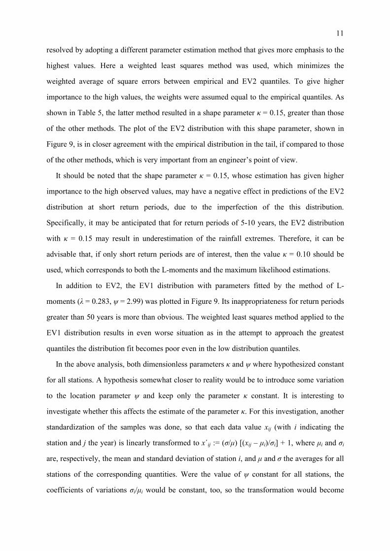
resolved by adopting a different parameter estimation method that gives more emphasis to the

highest values. Here a weighted least squares method was used, which minimizes the

weighted average of square errors between empirical and EV2 quantiles. To give higher

importance to the high values, the weights were assumed equal to the empirical quantiles. As

shown in Table 5, the latter method resulted in a shape parameter κ = 0.15, greater than those

of the other methods. The plot of the EV2 distribution with this shape parameter, shown in

Figure 9, is in closer agreement with the empirical distribution in the tail, if compared to those

of the other methods, which is very important from an engineer’s point of view.

It should be noted that the shape parameter κ = 0.15, whose estimation has given higher

importance to the high observed values, may have a negative effect in predictions of the EV2

distribution at short return periods, due to the imperfection of the this distribution.

Specifically, it may be anticipated that for return periods of 5-10 years, the EV2 distribution

with κ = 0.15 may result in underestimation of the rainfall extremes. Therefore, it can be

advisable that, if only short return periods are of interest, then the value κ = 0.10 should be

used, which corresponds to both the L-moments and the maximum likelihood estimations.

In addition to EV2, the EV1 distribution with parameters fitted by the method of L-

moments (λ = 0.283, ψ = 2.99) was plotted in Figure 9. Its inappropriateness for return periods

greater than 50 years is more than obvious. The weighted least squares method applied to the

EV1 distribution results in even worse situation as in the attempt to approach the greatest

quantiles the distribution fit becomes poor even in the low distribution quantiles.

In the above analysis, both dimensionless parameters κ and ψ where hypothesized constant

for all stations. A hypothesis somewhat closer to reality would be to introduce some variation

to the location parameter ψ and keep only the parameter κ constant. It is interesting to

investigate whether this affects the estimate of the parameter κ. For this investigation, another

standardization of the samples was done, so that each data value xij (with i indicating the

station and j the year) is linearly transformed to x΄ij := (σ/µ) [(xij – µi)/σi] + 1, where µi and σi

are, respectively, the mean and standard deviation of station i, and µ and σ the averages for all

stations of the corresponding quantities. Were the value of ψ constant for all stations, the

coefficients of variations σi/µi would be constant, too, so the transformation would become

12

x΄ij := xij/µi, which is the rescaling transformation that was already done in the previous

analysis. Similarly to the previous analysis, the corrected mean (equation (7)) was used while

for standard deviations the corrections due to Hershfield (1961) were applied.

The so transformed samples of the different stations were again unified and from the

unified series the parameters were re-estimated. Interestingly, all parameter estimation

methods resulted in virtually the same values of κ that are shown in Table 5 (the largest

difference was ±0.001). Moreover, the parameters λ and ψ were, too, almost equal to those of

Table 5 (largest difference ±2%).

6. Analysis of series of values over threshold

All previous analyses were performed on the annual maximum series. As discussed in the

Introduction, the probabilistic behaviour of the series over threshold can be theoretically

obtained from that of the annual maximum series. Here we show that this is also empirically

verified. The 168 series were rescaled by µ΄ as obtained from the annual maximum series and

then merged into a unified record. The empirical distribution of the unified record is shown in

the Pareto probability plot of Figure 10. The Pareto reduced variate that is used for the

horizontal axis is defined as yT := (T κ – 1) / κ with κ fixed to 0.15. The Pareto and exponential

distributions with parameters equal to those of the EV2 and EV1 distributions, respectively,

shown in Table 5, are also plotted in Figure 10. This figure shows that the same parameters

estimated from the unified annual maximum series are good for the Pareto distribution of the

unified series of values over threshold, so there is no need to re-estimate them. In addition, the

observations already made on Figure 9 about the superiority of the EV2 distribution fitted by

the method of least squares and the inappropriateness of the EV1 distribution are valid also

for, respectively, the Pareto and exponential distributions in Figure 10.

In addition to the Pareto probability plot of Figure 10, a log-log plot of rescaled rainfall

depth versus return period is given in Figure 11. The fact that both the empirical and fitted

theoretical distribution functions have an apparent curvature on this log-log plot suggest that

the power law relationship between rainfall depth and return period on a basis of values over

threshold (which has been called by Turcotte (1994) a fractal distribution and is equivalent to

13

the Fréchet distribution on a basis of annual maximum values) is inappropriate for modelling

rainfall extremes.

7. From EV1 to EV2 distribution

All above analyses converge to the conclusion that neither of the two-parameter special cases

of the GEV distribution, i.e. the Gumbel and Fréchet distributions, is appropriate for extreme

rainfall. On the contrary, the three-parameter EV2 distribution is an alternative much closer to

reality. In addition, they converge to the conclusion that the shape parameter of the EV2

distribution can be hypothesized to have a constant value κ = 0.15, regardless of the

geographical location of the raingauge station.

If the shape parameter of the EV2 distribution is fixed, the general handling of the

distribution becomes as simple as that of the EV1 distribution. For example, the estimation of

the remaining two parameters becomes similar to that of the EV1 distribution. That is, the

scale parameter can be estimated by the method of moments from

λ = c1 σ (8)

where c1 = κ / Γ(1 – 2 κ) – Γ 2(1 – κ) or c1 = 0.61 for κ = 0.15, while in the EV1 case c1 =

0.78. The relevant estimate for the method of L-moments is

λ = c2 λ2 (9)

where c2 = κ / [Γ(1 – κ)(2κ – 1)] or c2 = 1.23 for κ = 0.15, while in the EV1 case c2 = 1.443.

The estimate of the location parameter for both the method of moments and L-moments is

ψ = µ/λ – c3 (10)

where c3 = [Γ(1 – κ) – 1] / κ or c3 = 0.75 for κ = 0.15, while in the EV1 case c3 = 0.577.

If, in addition to λ and ψ, the shape parameter is to be estimated directly from the sample

(which is not advisable but it may be useful for comparisons) the following equations can be

used, which are approximations of the exact (but implicit) equations of the literature:

14

κ = 13 –

10.31 + 0.91 Cs + (0.91 Cs)2 + 1.8

(11)

κ = 8 c – 3 c2, c := ln 2ln 3 –

23 + τ3 (12)

The former corresponds to the method of moments and the resulting error is smaller than

±0.01 for –1 < κ < 1/3 (–2 < Cs< ∞). The latter corresponds to the method of L-moments and

the resulting error is smaller than ±0.008 for –1 < κ < 1 (–1/3 < τ3 < 1).

The construction of linear probability plots is also easy if κ is fixed. It suffices to replace in

the horizontal axis the Gumbel reduced variate zH := –ln(–ln H) with the GEV reduced variate

zH := [(-ln H)–κ – 1] / κ. Such plots are portrayed in Figure 12 for the same distributions

depicted in Figure 6 on Gumbel probability plots, but now for κ = 0.15. In addition to the

empirical and EV2 distributions, upper and lower prediction limits of the former, computed

by Monte Carlo simulation (e.g., Ripley, 1987, p. 176), have been plotted in this figure, which

demonstrate the high uncertainty of estimates for large return periods.

8. Conclusions and discussion

The conclusions of this extensive analysis based on 169 rainfall series with lengths 100-154

years and a total number of 18 065 station-years from stations in Europe and USA may be

summarized as follows.

1. Neither of the two-parameter special cases of the GEV distribution, i.e. the Gumbel and

Fréchet distributions, is appropriate for modelling annual maximum rainfall series. On the

contrary, the three-parameter EV2 distribution is a choice much closer to reality.

2. The shape parameter κ of the EV2 distribution is very hard to estimate on the basis of an

individual series, even in series with length 100 years or more. This is because of the

estimation bias and the large sampling variability of the estimators of κ, which was

demonstrated here using simulation. For example, for sample size m = 30 and κ = 0.15 the

method of moments estimates a κ almost zero and the method of L moments does not

reject the false hypothesis of EV1 distribution at 75% of cases (see first part of the study).

The analysis showed that even in the unified record with 18 065 values, the uncertainty in

estimating κ is large as different estimation methods yield different estimates of κ. The

15

most important conclusion, however, is that the observed variability in the values of κ in

the 169 series is almost entirely explained by statistical reasons as it is almost identical

with the sampling variability. This allows the hypothesis that the shape parameter of the

EV2 distribution is constant for all examined geographical zones, with value κ = 0.15.

3. The location parameter ψ of the EV2 distribution turned out to be fairly constant with a

mean value ψ = 3.54 (corresponding to κ = 0.15) and coefficient of variation as low as 0.13.

However, this small variation cannot be attributed to statistical reasons entirely as the

sampling variation seems to be slightly lower than that observed in the 169 historical

samples. This, however, is not a major problem as ψ can be estimated with relative

accuracy on the basis of an individual series.

4. The scale parameter λ of the EV2 distribution varies with the station location and there is

no need to seek a generalized law about it as it can be estimated with relative accuracy on

the basis of an individual series.

5. The behaviour of the examined series over threshold turns out to be fully consistent with

that of the annual maximum series, as the same parameter values of the EV2 distribution of

the latter are equally good for the Pareto distribution of the former. Thus, the statistical

analysis of either the annual maximum series or the series over threshold suffices to know

the behaviour of both.

6. In engineering practice, the handling of the EV2 distribution can be as easy as that of the

EV1 distribution if the shape parameter of the former is fixed to the value κ = 0.15. The

parameter estimation is virtually the same (only some constants change) and very similar

linear probability plots can be constructed (the Gumbel reduced variate zH := –ln(–ln H)

should be replaced with the GEV reduced variate zH := [(–ln H)–0.15 – 1] / 0.15, or in case

of series over threshold with the Pareto reduced variate yT := (T 0.15 – 1) / 0.15. If the

linearity of the plot is not necessary, a log-log plot of distribution quantile versus return

period is a simpler choice.

In a recent study, Koutsoyiannis (1999) revisited Hershfield’s (1961) data set (95 000

station-years from 2645 stations) and showed that this can be described by the EV2

distribution with κ = 0.13. The plot of Figure 13, indicates that the value κ = 0.15 that is

16

proposed in the present study can be acceptable for that data set too. This enhances the trust

that an EV2 distribution with κ = 0.15 can be thought of as a generalized model appropriate

for mid latitude areas of the north hemisphere. The present analyses do not confirm

Hershfield’s (1965) observation that arid areas tend to have higher relative extremes (ratios of

maximum to mean or standard deviation) than areas with heavy rainfall, which as

Koutsoyiannis (1999) showed, is equivalent to a negative correlation of κ with mean. Before a

concrete conclusion on this issue can be drawn, long records from other geographical zones,

especially tropical and south hemisphere ones, should be explored.

The results of this study also converge with other recent studies such as those by Chaouche

(2001), Chaouche et al. (2002), Coles et al., (2003) and Sisson et al. (unpublished), which all

verify the EV2/Pareto behaviour in the tail of the distribution of rainfall extremes and exclude

the possibility of EV1/exponential behaviour. Particularly, Chaouche (2001) exploited a data

base of 200 rainfall series of various time steps (month, day, hour, minute) from the five

continents, each including more than 100 years of data. Using multifractal analyses he showed

that (a) a Pareto type law describes the rainfall amounts for large return periods; (b) the

exponent of this law is scale invariant over scales greater than an hour; and (c) this exponent

is almost space invariant.

Acknowledgements The data from USA belong to the United States Historical Climatology Network (USHCN)

and are available online from http://lwf.ncdc.noaa.gov/oa/climate/research/ushcn/ushcn.html. The data from the

UK belong to the Land Surface Observation Data of the Met Office and were kindly provided through download

from the web site http://badc.nerc.ac.uk/ of the British Atmospheric Data Centre (BADC). The data from France

were kindly provided by Philippe Bois (Laboratoire d’Etudes des Transferts en Hydrologie et Environnement,

Ecole Nationale Supérieure d’Hydraulique et de Mécanique de Grenoble; LTHE-ENSHMG). The data from Italy

were kindly provided by Alberto Montanari (University of Bologna). The record from Greece was originated

from an earlier study (Koutsoyiannis and Baloutsos, 2000) and was updated with data values of the recent years

kindly provided by Vasso Kotroni (National Observatory of Athens). Thanks are also due to Christian Onof

(Imperial College) and Charles Obled (LTHE-ENSHMG) for their help in seeking datasets from UK and France

and for providing useful information and comments. With the editor’s help, the paper was so fortunate as to

bring two very encouraging, constructive and detailed reviews by Alberto Montanari and an anonymous

reviewer, which improved the paper substantially.

17

References

Chaouche K. (2001) Approche Multifractale de la Modelisation Stochastiqueen Hydrologie, thèse, Ecole

Nationale du Génie Rural, des Eaux et des Forêts, Centre de Paris (http://www.engref.fr/

thesechaouche.htm).

Chaouche, K., Hubert, P., Lang, G. (2002) Graphical characterisation of probability distribution tails, Stochastic

Environmental Research and Risk Assessment, 16(5), 342-357.

Chow V.T., Maidement D.R and Mays L.W.(1988), Applied Hydrology, McGraw-Hill, New York.

Coles, S., Pericchi, L. R., and Sisson, S., (2003) A fully probabilistic approach to extreme rainfall modeling,

Journal of Hydrology, 273(1-4), 35-50.

Hershfield, D. M. (1961) Estimating the probable maximum precipitation, Proc. ASCE, J. Hydraul. Div.,

87(HY5), 99-106.

Hershfield, D. M. (1965) Method for estimating probable maximum precipitation, J. American Waterworks

Association, 57, 965-972.

Hosking, J. R. M. (1990) L-moments: Analysis and estimation of distributions using linear combinations of

order statistics, J. R. Stat. Soc., Ser. B, 52, 105-124.

Jenkinson, A. F. (1955) The frequency distribution of the annual maximum (or minimum) value of

meteorological elements, Q. J. Royal Meteorol. Soc., 81, 158-171.

Jenkinson, A. F. (1969) Estimation of maximum floods, World Meteorological Organization, Technical Note No

98, ch. 5, 183-257.

Koutsoyiannis, D. (1999) A probabilistic view of Hershfield’s method for estimating probable maximum

precipitation, Water Resources Research, 35(4), 1313-1322.

Koutsoyiannis, D., and Baloutsos, G. (2000) Analysis of a long record of annual maximum rainfall in Athens,

Greece, and design rainfall inferences, Natural Hazards, 22(1), 31-51.

National Research Council (1994) Estimating Bounds on Extreme Precipitation Events, National Academy Press,

Washington.

Ripley, B. D. (1987) Stochastic Simulation, Wiley, New York.

Sisson, S. A., Pericchi, L. R., and Coles, S. (unpublished) A case for a reassessment of the risks of extreme

hydrological hazards in the Caribbean (www.maths.unsw.edu.au/~scott/papers/paper_caribbean_abs.html)

Turcotte, D. L. (1994) Fractal theory and the estimation of extreme floods, J. Res. Natl. Inst. Stand. Technol.,

99(4), 377-389.

18

Table 1 General characteristics of raingauges of the different geographical zones.

Geographical zone

1 2 3 4 5 6 Total

Number of stations 104 19 15 3 24 4 169

Record length min 100 100 100 100 100 128 100

max 130 131 122 103 130 154 154

Number of station-years 10942 2012 1610 304 2624 573 18065

Elevation (m) min 3 3 11 376 6 3

max 1867 917 2078 1870 107 2078

Table 2 General characteristics of the top ten, in terms of record length, raingauges.

Name

Zone/Country

/State

Latitu-

de (oN)

Longi-

tude (o)

Eleva-

tion (m)

Record

length

Start

year

End

year

Years with missing

values

Florence 6/Italy 43.80 11.20 40 154 1822* 1979 1874-77

Genoa 6/Italy 44.40 8.90 21 148 1833 1980

Athens 6/Greece 37.97 23.78 107 143 1860 2002

Charleston City 2/USA/SC 32.79 –79.94 3 131 1871 2001

Oxford 5/UK 51.72 –1.29 130 1853 1993 1930, 1933,1961-69

Cheyenne 1/USA/WY 41.16 –104.82 1867 130 1871 2001 1877

Marseille 6/France 43.45 5.20 6 128 1864 1991

Armagh 5/UK 54.35 –6.65 128 1866 1993

Savannah 2/USA/GA 32.14 –81.20 14 128 1871 2001 1969-71

Albany 1/USA/NY 42.76 –73.80 84 128 1874 2001

* Record starts in 1813 but values prior to 1822 are incorrect.

19

Table 3 Averages and ranges of statistical characteristics of annual maximum daily rainfall series for the

different geographical zones.

Geographical zone

1 2 3 4 5 6 Total

Sample mean, µ (mm) min 34.2 65.3 19.1 31.8 31.3 48.5 19.1

mean 65.7 91.0 36.5 39.4 36.1 68.9 61.4

max 90.1 109.0 75.3 48.7 46.4 110.9 110.9

Sample maximum, xmax (mm) min 88.4 146.8 40.1 84.3 54.1 140.0 40.1

mean 175.8 265.7 83.9 125.2 89.7 225.4 165.8

max 429.5 490.0 157.0 201.2 130.3 389.2 490.0

Coefficient of variation, Cv min 0.26 0.32 0.31 0.35 0.26 0.35 0.26

mean 0.38 0.42 0.36 0.41 0.34 0.42 0.38

max 0.68 0.57 0.47 0.47 0.45 0.48 0.68

Coefficient of skewness, Cs min 0.58 0.89 0.83 1.08 0.55 1.65 0.55

mean 1.69 1.81 1.19 1.93 1.70 1.92 1.67

max 4.94 3.89 1.69 3.32 3.22 2.03 4.94

L-coefficient of variation, τ2 min 0.14 0.18 0.16 0.19 0.14 0.18 0.14

mean 0.19 0.21 0.19 0.21 0.17 0.22 0.19

max 0.26 0.25 0.25 0.22 0.22 0.24 0.26

L-coefficient of skewness, τ3 min 0.12 0.16 0.14 0.16 0.15 0.22 0.12

mean 0.24 0.26 0.21 0.23 0.24 0.26 0.24

max 0.43 0.38 0.26 0.29 0.35 0.28 0.43

20

Table 4 Averages over all raingauges and dispersion characteristics of the parameters of the GEV

distribution as estimated by three different methods from the annual maximum daily rainfall series.

Estimation method

Parameter Max likelihood Moments L-Moments

κ Mean 0.103 0.052 0.103

Standard deviation 0.080 0.079 0.085

Min –0.061 –0.121 –0.080

Max 0.303 0.238 0.373

Percent positive 91% 74% 92%

λ Mean 15.39 16.64 15.52

Standard deviation 5.63 6.31 5.81

Min 4.95 5.16 4.86

Max 31.08 34.89 32.13

ψ Mean 3.36 3.14 3.34

Standard deviation 0.42 0.44 0.43

Min 2.54 2.07 2.42

Max 4.48 4.44 4.47

Table 5 Parameters of the EV2 distribution as estimated by four different methods from the unified record

of all 169 annual maximum rescaled daily rainfall series (18 065 station-years).

Estimation method

Parameter Max likelihood Moments L-moments Weighted least squares

κ 0.093 0.126 0.104 0.148

λ 0.258 0.248 0.255 0.236

ψ 3.24 3.36 3.28 3.54

21

Zone 6 (Mediterranean)

Zone 5 (UK)

Zone 1 (NE USA)

Zone 3 (NW USA)

Zone 4 (SW USA) Zone 2 (SE USA)

105th meridian

35th parallel

Figure 1 Geographical locations of raingauges.

22

10

100

1000

10 100 1000

Sample mean (mm)

Obs

erve

d m

axim

um (m

m)

1 2 34 5 6

Zone

slope = 1.08

Figure 2 Plot of the sample mean and maximum, over the observation period, of each annual maximum

daily rainfall series for the six different geographical zones.

0.1

0.15

0.2

0.25

0.3

0.35

0.4

0.45

0 20 40 60 80 100 120

Mean of annual maximum daily rainfall (mm)

L-va

riatio

n, L

-ske

wne

ss

L-variationL-skewness

Figure 3 Plot of the L-variation and L-skewness coefficients vs. the mean of the annual maximum daily

rainfall series.

23

0.1

0.15

0.2

0.25

0.3

0.35

0.4

0.45

0.1 0.15 0.2 0.25 0.3

L-variation

L-sk

ewne

ss

1 2 34 5 6

Zone

Figure 4 Plot of L-skewness vs. L-variation coefficient for the annual maximum daily rainfall series for the

six different geographical zones.

0.1

0.15

0.2

0.25

0.3

0.35

0.4

0.45

0.1 0.15 0.2 0.25 0.3

L-variation

L-sk

ewne

ss

Figure 5 Plot of L-skewness vs. L-variation coefficient for 169 synthetic samples with lengths and means

equal to those of the historical records, generated from the EV2 distribution with shape parameter κ = 0.103

and location parameter ψ = 3.34.

24

0

50

100

150

200

250

300

-2 -1 0 1 2 3 4 5 6Gumbel reduced variate

Rai

nfal

l dep

th (m

m) T= 1.01 1.2 2 5 10 20 50 100 200

(a)

0

20

40

60

80

100

-2 -1 0 1 2 3 4 5 6Gumbel reduced variate

Rai

nfal

l dep

th (m

m) T= 1.01 1.2 2 5 10 20 50 100 200

(b)

0

50

100

150

200

250

-2 -1 0 1 2 3 4 5 6Gumbel reduced variate

Rai

nfal

l dep

th (m

m) T= 1.01 1.2 2 5 10 20 50 100 200

(c)

0

25

50

75

100

125

150

-2 -1 0 1 2 3 4 5 6Gumbel reduced variate

Rai

nfal

l dep

th (m

m) T= 1.01 1.2 2 5 10 20 50 100 200

(d)

Figure 6 EV2 (continuous lines) and EV1 (dotted lines) distributions fitted by the method of L-moments

and comparison with the empirical distribution (crosses) for the annual maximum daily rainfall series of (a)

Charleston City, USA/SC; (b) Oxford, UK (c) Marseille, France; and (d) Florence, Ximeniano Observatory,

Italy (Gumbel probability plots).

25

0

50

100

150

200

250

300

350

400

450

-2 0 2 4 6 8 10 12Gumbel reduced variate

Rai

nfal

l dep

th (m

m)

EmpiricalEV2/L-momentsEV2/Max likelihoodEV2/MomentsEV1/L-moments

1.01

1.2

2 5 10 20 50 100

200

500

1000

2000

5000

1000

020

000

5000

0

1000

00Return period, years

Estimated PMP value ↑

Figure 7 EV2 and EV1 distributions fitted by several methods and comparison with the empirical

distribution for the annual maximum daily rainfall series of Athens, National Observatory, Greece (Gumbel

probability plot). The PMP value (424.1 mm) was estimated by Koutsoyiannis and Baloutsos (2000).

26

0

0.2

0.4

0.6

0.8

1

0.1 0.15 0.2 0.25 0.3 0.35τ 2

F τ2(τ

2 )

0

0.2

0.4

0.6

0.8

1

0.2 0.4 0.6 0.8C v

F cv(c

v )0

0.2

0.4

0.6

0.8

1

0 0.2 0.4 0.6τ 3

F τ3(τ

3 )

0

0.2

0.4

0.6

0.8

1

0 2 4 6 8c s

F cs(c

s )

0

0.2

0.4

0.6

0.8

1

-0.2 -0.1 0 0.1 0.2 0.3 0.4 0.5 0.6κ

F κ(κ

)

0

0.2

0.4

0.6

0.8

1

0 2 4 6 8υ = x max / µ

F υ(υ

)

0

0.2

0.4

0.6

0.8

1

0 0.1 0.2 0.3 0.4 0.5τ 4

F τ4(τ

4 )

0

0.2

0.4

0.6

0.8

1

2 3 4 5ψ

F ψ(ψ

)

Figure 8 Empirical distribution functions of several dimensionless sample statistics (coefficients of

variation τ2 and Cv, skewness τ3 and Cs, and kurtosis τ4; ratio of maximum value xmax to mean value µ; and

L-moments estimates of parameters κ and ψ of the GEV distribution), as computed from either: the 169

historical annual maximum daily rainfall series (thick continuous lines); 169 synthetic samples with lengths

and means equal to those of historical series generated from the GEV distribution with constant shape

parameter κ = 0.103 and location parameter ψ = 3.34 (dotted lines); and 169 synthetic samples with lengths

and means equal to those of historical series generated from the GEV distribution with shape parameter κ

and location parameter ψ varying following uniform distributions (dashed lines).

27

0

1

2

3

4

5

6

7

8

-2 0 2 4 6 8 10 12Gumbel reduced variate

Res

cale

d ra

infa

ll dep

th EmpiricalEV2/Least squaresEV2/MomentsEV2/L-momentsEV2/Max likelihoodEV1/L-moments

1.01

1.2

2 5 10 20 50 100

200

500

1000

2000

5000

1000

020

000

5000

010

0000Return period, years

Figure 9 EV2 and EV1 distributions fitted by several methods and comparison with the empirical

distribution for the unified record of all 169 annual maximum rescaled daily rainfall series (18 065 station-

years).

28

0

1

2

3

4

5

6

7

8

0 2 4 6 8 10 12 14 16 18 20 22 24 26 28 30 32Pareto reduced variate

Res

cale

d ra

infa

ll de

pth

EmpiricalPareto/Least squaresPareto/MomentsPareto/L-momentsPareto/Max likelihoodExponential/L-moments

2 5 10 20 50 100

200

500

1000

2000

5000

1000

0

2000

0

5000

0

1000

00

Return period, years

Figure 10 Empirical distribution of the union of the 168 series of rescaled rainfall depths over threshold

(17922 station-years) in comparison with the Pareto distribution with parameters estimated from the unified

series of annual maxima, shown in Table 5 (Pareto probability plot with κ = 0.15).

1 10 100 1000 10000 100000

Return period

Res

cale

d ra

infa

ll de

pth

EmpiricalPareto/Least squaresPareto/L-momentsExponential/L-moments

0.5

1

2

5

10

2 5

Figure 11 Empirical and Pareto distributions of the union of the 168 series of values over threshold (17922

station-years) as in Figure 10 but in a double logarithmic plot of rescaled rainfall depths vs. return period.

29

0

100

200

300

400

-2 0 2 4 6 8GEV reduced variate

Rai

nfal

l dep

th (m

m)

T= 1.01 1.2 2 5 10 20 50 100 200

(a)

0

25

50

75

100

125

-2 0 2 4 6 8GEV reduced variate

Rai

nfal

l dep

th (m

m)

T= 1.01 1.2 2 5 10 20 50 100 200

(b)

0

50

100

150

200

250

300

-2 0 2 4 6 8GEV reduced variate

Rai

nfal

l dep

th (m

m)

T= 1.01 1.2 2 5 10 20 50 100 200

(c)

0

50

100

150

200

-2 0 2 4 6 8GEV reduced variate

Rai

nfal

l dep

th (m

m)

T= 1.01 1.2 2 5 10 20 50 100 200

(d)

Figure 12 Empirical distributions (crosses), EV2 distributions (continuous lines), and 95% Monte Carlo

prediction limits for the empirical distribution (dashed lines) of the annual maximum daily rainfall series of

(a) Charleston City, USA/SC; (b) Oxford, UK (c) Marseille, France; and (d) Florence, Italy, as in Figure 6

but in GEV plot with κ = 0.15. The EV2 distribution was fitted by the method of L-moments assuming

fixed κ = 0.15.

30

0

2

4

6

8

10

12

14

16

-2 3 8 13 18 23 28 33GEV reduced variate

Her

shfie

ld-s

tand

ardi

sed

rain

fall d

epth

Empiricalκ = 0.15κ = 0.13 (Koutsoyiannis, 1999)

1.01

1.2

2 5 10 20 50 100

200

500

1000

2000

5000

1000

0

2000

0

5000

0

1000

00Return period, years

Figure 13 Empirical distribution of standardized rainfall depth k for Hershfield’s (1961) data set (95 000

station-years from 2645 stations), as determined by Koutsoyiannis (1999), and fitted EV2 distributions with

κ = 0.13 (Koutsoyiannis, 1999) and κ = 0.15 (present study) (GEV probability plots with κ = 0.15).