Embed Size (px)
Citation preview

University of Pennsylvania University of Pennsylvania
ScholarlyCommons ScholarlyCommons
Statistics Papers Wharton Faculty Research
7-2017
Customer Acquisition via Display Advertising Using Multi-Armed Customer Acquisition via Display Advertising Using Multi-Armed
Bandit Experiments Bandit Experiments
Eric M. Schwartz The University Of Michigan
Eric T. Bradlow University of Pennsylvania
Peter S. Fader University of Pennsylvania
Follow this and additional works at: https://repository.upenn.edu/statistics_papers
Part of the Business Commons, and the Statistics and Probability Commons
Recommended Citation Recommended Citation Schwartz, E. M., Bradlow, E. T., & Fader, P. S. (2017). Customer Acquisition via Display Advertising Using Multi-Armed Bandit Experiments. Marketing Science, 36 (4), 500-522. http://dx.doi.org/10.1287/mksc.2016.1023
This paper is posted at ScholarlyCommons. https://repository.upenn.edu/statistics_papers/6 For more information, please contact [email protected].

Customer Acquisition via Display Advertising Using Multi-Armed Bandit Customer Acquisition via Display Advertising Using Multi-Armed Bandit Experiments Experiments
Abstract Abstract Firms using online advertising regularly run experiments with multiple versions of their ads since they are uncertain about which ones are most effective. During a campaign, firms try to adapt to intermediate results of their tests, optimizing what they earn while learning about their ads. Yet how should they decide what percentage of impressions to allocate to each ad? This paper answers that question, resolving the well-known “learn-and-earn” trade-off using multi-armed bandit (MAB) methods. The online advertiser’s MAB problem, however, contains particular challenges, such as a hierarchical structure (ads within a website), attributes of actions (creative elements of an ad), and batched decisions (millions of impressions at a time), that are not fully accommodated by existing MAB methods. Our approach captures how the impact of observable ad attributes on ad effectiveness differs by website in unobserved ways, and our policy generates allocations of impressions that can be used in practice. We implemented this policy in a live field experiment delivering over 750 million ad impressions in an online display campaign with a large retail bank. Over the course of two months, our policy achieved an 8% improvement in the customer acquisition rate, relative to a control policy, without any additional costs to the bank. Beyond the actual experiment, we performed counterfactual simulations to evaluate a range of alternative model specifications and allocation rules in MAB policies. Finally, we show that customer acquisition would decrease by about 10% if the firm were to optimize click-through rates instead of conversion directly, a finding that has implications for understanding the marketing funnel.
Keywords Keywords multi-armed bandit, online advertising, field experiments, A/B testing, adaptive experiments, sequential decision making, explore-exploit, earn-and-learn reinforcement learning, hierarchical models
Disciplines Disciplines Business | Statistics and Probability
This journal article is available at ScholarlyCommons: https://repository.upenn.edu/statistics_papers/6

Electronic copy available at: http://ssrn.com/abstract=2368523
Customer Acquisition via Display AdvertisingUsing Multi-Armed Bandit Experiments
Forthcoming at Marketing Science
Eric M. Schwartz, Eric T. Bradlow, and Peter S. Fader ⇤
March 29, 2016
Abstract
Firms using online advertising regularly run experiments with multiple versions of theirads since they are uncertain about which ones are most effective. Within a campaign, firmstry to adapt to intermediate results of their tests, optimizing what they earn while learningabout their ads. But how should they decide what percentage of impressions to allocate to eachad? This paper answers that question, resolving the well-known “learn-and-earn” trade-offusing multi-armed bandit (MAB) methods. The online advertiser’s MAB problem, however,contains particular challenges, such as a hierarchical structure (ads within a website), attributesof actions (creative elements of an ad), and batched decisions (millions of impressions at atime), that are not fully accommodated by existing MAB methods. Our approach captureshow the impact of observable ad attributes on ad effectiveness differs by website in unobservedways, and our policy generates allocations of impressions that can be used in practice.
We implemented this policy in a live field experiment delivering over 700 million ad im-pressions in an online display campaign with a large retail bank. Over the course of two months,our policy achieved an 8% improvement in the customer acquisition rate, relative to a controlpolicy, without any additional costs to the bank. Beyond the actual experiment, we performedcounterfactual simulations to evaluate a range of alternative model specifications and allocationrules in MAB policies. Finally, we show that customer acquisition would decrease about 10%if the firm were to optimize click through rates instead of conversion directly, a finding that hasimplications for understanding the marketing funnel.
Keywords: multi-armed bandit, online advertising, field experiments, A/B testing, adaptive experiments, sequen-tial decision making, explore-exploit, earn-and-learn reinforcement learning, hierarchical models.
* Eric M. Schwartz is an Assistant Professor of Marketing at the Stephen M. Ross School of Business at theUniversity of Michigan. Eric T. Bradlow is the K. P. Chao Professor; Professor of Marketing, Statistics, andEducation; Vice Dean and Director of Wharton Doctoral Programs; and Co-Director of the Wharton CustomerAnalytics Initiative at the University of Pennsylvania. Peter S. Fader is the Frances and Pei-Yua Chia Professor;Professor of Marketing; and Co-Director of the Wharton Customer Analytics Initiative at the University of Penn-sylvania. This paper is based on the first author’s dissertation. All correspondence should be addressed to Eric M.Schwartz: [email protected], 734-936-5042; 701 Tappan Street, R5472, Ann Arbor, MI 48109-1234.

Electronic copy available at: http://ssrn.com/abstract=2368523
1 Introduction
Business experiments have a long history in marketing. As digital environments facili-
tate randomization, controlled experiments, known as A/B tests, have become an increasingly
popular part of a firm’s analytics capabilities (Anderson and Simester 2011; Davenport 2009;
Donahoe 2011; Hauser et al. 2014; Urban et al. 2014). As a result, many interactive marketing
firms are continuously testing and learning in their market environments; however they are
bypassing a more profitable option: firms could be earning while learning.
One domain frequently using such testing is online advertising. Firms typically handle
this earning vs. learning (or explore-exploit) trade-off in two phases, test then rollout. They
equally allocate impressions to each ad version (explore phase), and after stopping the test,
they shift all future impressions to the best performing ad (exploit phase). But it is impossible
to know the optimal test phase length in advance. Instead of a discrete switch from exploration
(learning) to exploitation (earning), firms should simultaneous mix the two and change the mix
with a smooth transition from one to the other (earning while learning). In practical terms, this
problem is formulated as, how should a firm decide what percentage of impressions to allocate
to each online ad on an ongoing basis to maximize earning while continuously learning?
We focus on solving this problem, but first we emphasize that it is not unique to online
advertisers; it belongs to a much broader class of sequential allocation problems that marketers
have faced for years across countless domains. Many other activities – sending emails or direct
mail catalogs, providing customer service, designing websites – can be framed as sequential
adaptive experiments. All of these problems are structured around the following questions:
Which targeted marketing action should we take, when should we take them, and with which
customers and in which contexts, should we test such actions? With limited funds, the firm
faces the resource allocation problem: how can they exploit data they have about their market-
1

Electronic copy available at: http://ssrn.com/abstract=2368523
ing actions and further explore those actions’ effectiveness to reduce their uncertainty?
We frame this class of problems as a multi-armed bandit (MAB) (Robbins 1952; Thompson
1933). The MAB problem (formally defined later) is a classic adaptive experimentation and
dynamic optimization problem. While various MAB methods have been developed, they fall
short of addressing the richness of the online advertising problem we present here.
First, within online advertising, we focus on optimizing the advertiser’s resource allocation
over time across many ad creatives and websites by sequentially learning about ad performance.
This allows us to maximize customer acquisition rates by testing many ads on many websites
while learning which ad works best on each website. Our findings have immediate marketing
implications, as they emphasize the importance of the interaction between context and ad cre-
ative in optimizing online advertising campaigns. This problem relates to other work at the
intersection of online advertising, online content optimization, and MAB problems (Agarwal
et al. 2008; Hauser et al. 2014; Scott 2010; Urban et al. 2014). Like those studies, we downplay
what the firm learns about specific ad characteristics (e.g., which ad message or which format
works best?) in favor of learning purely as a means to earning as much as possible.
We go beyond sequentially testing ad performance; we explicitly test the resulting MAB
policy’s effectiveness in a real-time and live randomized control trial. We randomly assign each
observation (i.e., consumer-ad impression) to be treated by either our proposed MAB policy or
a control policy (balanced experiment). Using the data collected, we run counterfactual policy
simulations to understand how various MAB methods would have performed in this setting. By
directly comparing distinct methodological approaches, this research provides a broader study
of MAB policies in marketing. We also study how robust these methods are to changes in our
problem setting.
Second, from a methodological perspective, we propose a method for a version of the MAB
2

that is new to the literature: a hierarchical, attribute-based, batched MAB policy. The key
novel component is incorporating unobserved heterogeneity by using a hierarchical, partially
pooled model. While some recent work has incorporated attributes into actions and/or batched
decisions (Chapelle and Li 2011; Dani et al. 2008; Keller and Oldale 2003; Rusmevichientong
and Tsitsiklis 2010; Scott 2010), no prior work has considered a MAB with action attributes
and unobserved heterogeneity; yet the combination is central to the practical problem facing an
online advertiser. By using hierarchical modeling with partial pooling in our MAB policy, we
leverage information across all websites to allocate impressions across ads within any single
website. We quantify the value of accounting for unobserved heterogeneity in responsiveness
to ads and their attributes across websites.
We implement our proposed MAB policy in a large-scale, adaptive field experiment in
collaboration with a large retail bank focused on direct marketing to acquire customers. The
field experiment generated data over two months in 2012, including more than 750 million ad
impressions, which featured 12 unique banner ads that were described by two attributes (three
different sizes and four creative concepts), yielding 532 unique units of observations (website-
ad combinations).
We apply an approach featuring a principle called Thompson Sampling (Thompson 1933)
(also known as randomized probability matching, Chapelle and Li 2011; Granmo 2010; May
et al. 2011; Scott 2010). The principle of Thompson Sampling (TS) is simply stated: the prob-
ability that an action is believed to be optimal determines the proportion of resources allocated
to that action (Thompson 1933). We discuss its details and its theoretical properties later.
While using TS with a heterogeneous response model is one approach, we also examine a
range of alternative MAB policies (models and allocation rules) from the literature. We hope
to expose the marketing and management science audience to a wider range of MAB methods
3

than have previously been compared.
Our findings suggest that “one policy does not fit all” settings equally well. We find that
the choice of model specification, in particular whether to use an pooled, unpooled, or partially
pooled model, may matter more than the specific choice of MAB algorithm. While we pro-
pose a partially pooled model with the TS allocation rule, we find that an unpooled modeling
approach can yield even better results in our particular setting. For this unpooled approach, we
also show how a set of alternative MAB allocation rules can achieve similar levels of perfor-
mance. Nevertheless, we find there is usually lower risk (i.e., variance of optimized reward)
when using the proposed partially pooled model with TS.
In addition to improving the advertiser’s ability to solve their optimization problem, we
contribute to our understanding of the growing industry of online display advertising. Previous
research has examined and questioned the effectiveness of display advertising (Goldfarb and
Tucker 2011; Hoban and Bucklin 2015; Lambrecht and Tucker 2013; Manchanda et al. 2006;
Reiley et al. 2011). Instead of focusing on that measurement question, we focus on the problem
of running ad experiments more profitably.
The rest of the paper is structured as follows. The next section provides institutional details
of the field experiment design. In Section 3, we formalize the advertiser’s problem into a
MAB, and in Section 4, we describe our two-part approach to solving the full MAB problem:
a heterogeneous generalized linear model and the TS allocation rule. The remaining sections
cover the empirical performance in the live field experiment and a series of counterfactual
simulations for alternative policies.
4

2 Field Experiment Setup and Institutional Details
To design and implement our field experiment, we worked with a major U.S. financial
services company running a marketing campaign for one of its consumer banking products.
The campaign delivered over 750 million impressions over 62 days, from June 6 to August 6,
2012. The bank’s creative agency and media buying agency had already decided on four ad
concepts and formatted them for three standard ad sizes.
The ad buyer purchased media across the Internet at the level of media placements. These
media placements, often called lines of media, are a combination of many factors. A media
placement is first described by its publisher, either large ad networks/exchanges (e.g., Google
and Yahoo), or specific websites (e.g., Time.com and Bankrate.com). Table 1 lists all publishers
involved in the campaign and field experiment. Second, a media placement can refer to a
description of the audience defined broadly (e.g., all visitors to a publisher’s site), to a targeted
group (e.g., websites attracting visitors at least 45 years old), or even to a retargeted group (e.g.,
only cookies associated with individuals who visited the advertised financial product’s website
in the past 30 days but have not yet applied for an account). Third, the media placement also
considers the size of the ad such as one of the these three industry standard formats, 300x250,
160x600, or 728x90 pixels. For exposition, we will refer to the size of the ad as an attribute of
the ad rather than as an attribute of the paid media placement. The impressions already were
purchased for specific media placements, so we will decide how many impressions each ad
creative receives within each media placement. As a result, we will not affect the cost of the
campaign, only the return on advertising expenditure.
[INSERT TABLE 1 ABOUT HERE]
The experiment yielded 532 units of observations (per period), which are unique combi-
5

nations of website, ad size, and ad concept. Of these, 348 observations come from publishers
with all three ad sizes available, 128 observations come from publishers with two ad sizes, and
56 observations come from publishers with only one ad size. Period refers to approximately
one week, the time between the updates we made in the adaptive field experiment.
For each observation per period, we observed the total number of ad impressions delivered
(impressions), whether the consumer clicked on that ad (clicks), and whether the consumer
who viewed the ad impression was acquired (conversions). We use the terms conversion and
acquisition interchangeably, and in this consumer banking context, it means that a customer
applied for a savings account.
Table 2 summarizes the media placements showing volume of impressions, clicks, and con-
versions by media category, which represents classes such as portal, contextual, and retargeting.
For example, as a publisher, Google appears in many media placements across different cate-
gories. Other publishers have placements in a single category, such as the BBC or Time Inc.,
with placements appearing only in news and information category.
[INSERT TABLE 2 ABOUT HERE]
While conversion and click-through rates differed by ad sizes and ad concepts, we find that
the heterogeneity in conversion rates across media placements is greater than the differences
across ads. This suggests that the context or customer segment may have more explanatory
power in predicting conversion than the ads, whose differential effects we intended to learn.
The histogram (Figure 1) shows the marginal distribution of these conversion rates over the
532 observations by the end of the experiment, and the scatter plot (Figure 2) illustrates the
joint distribution of conversions and total impression volume after the 62 days.
[INSERT FIGURE 1 ABOUT HERE]
6

[INSERT FIGURE 2 ABOUT HERE]
The heterogeneity of conversion rates across media placements is expected. Each media
placement represents a slice of the Internet browsing population, i.e., customers likely sharing
interests, behaviors, or demographics. Those different customer segments arise either indirectly
due to the website’s content, or directly based on the media placement’s targeting methods. In
addition to the different consumer segments, different media placements will vary with respect
to their effectiveness. Table 3 reveals that across placements, the conversion rates move to-
gether, as seen by the relatively high correlations of conversion rates across the four ad concepts
by media placement.
[INSERT TABLE 3 ABOUT HERE]
However, the nature of heterogeneity is even more complicated than different levels of
conversion rates would imply. Since context matters in advertising, it is reasonable to expect
an interaction between ad concept (e.g., design, call to action, etc.) and the media placement
(e.g., consumer segment). Indeed, these interactions do occur in the data collected (Table 3),
and our methods will allow for us to capture these effects.
3 Formalizing Online Display Advertising as a Multi-Armed Bandit Problem
3.1 Preliminaries
We translate the aforementioned advertiser’s problem into MAB language, formally defin-
ing the MAB problem and proposing our approach to solving it. Compared to the basic MAB
problem most commonly seen in the literature, our MAB problem differs along three key di-
mensions: attribute-based actions, batched decision making, and heterogeneity across contexts
in expected reward and in attribute importance.
7

The firm has ads, k = 1, . . . , K, that it can serve on any or all of a set of websites, j =
1, . . . , J . Let impressions be denoted by mjkt and conversions, by yjkt, from ad k on website
j in period t. Each ad’s unknown conversion rate, µjk, is assumed to be stationary over time
(discussed later), but is specific to each website-ad combination.
The ad conversion rates are not only unknown, but they may be correlated since they are
functions of unknown common parameters denoted by ✓, and a common set of d ad attributes.
Hence, the MAB is attribute-based. Ad k’s attributes xk may represent size, concept, message
appeal, image, or other aesthetics. The vector xk corresponds to the kth row of the whole
attribute structure, X , which is the design matrix of size K ⇥ d. In our empirical example, the
attributes are two nominal categorical variables: size (3 levels) and concept (4 levels), so we
have K = d = 12. Despite the low-dimensional attribute structure in our empirical example,
we maintain a more general notation here. To further emphasize the actions’ dependence on
those common parameters, we use the notation µjk(✓), but we note that µjk is really a function
of both xk and a subset of parameters, the corresponding coefficients, in ✓.
Since many observations are allocated simultaneously instead of one observation at-a-time,
the problem is a batched MAB (Chick and Gans 2009; Perchet et al. 2015). For each decision
period and website, the firm has a budget of Mjt =PK
k=1
mjkt impressions. In the problem
we address, this budget constraint is taken as given and exogenous due to previously arranged
media contracts, but the firm is free to decide what proportion of those impressions will be
allocated to each ad. This proportion is wjkt, wherePK
k=1
wjkt = 1.
In each decision period, the firm has the opportunity to make different allocations of impres-
sions of K ads across each of J different websites. This ad-within-website structure implies the
problem is hierarchical. Since each ad may perform differently depending on which website it
appears, we allow an ad’s conversion rate to vary by using website-specific attribute importance
8

parameters, �j . Then the impact of the ad attributes on the conversion rate can be described by
a common generalized linear model (GLM), µjk(✓) = h
�1
(x
0k�j), where h is the link function
(e.g., logit, probit).
3.2 Optimization Problem
The firm’s objective is to maximize the expected total number of customers acquired by
serving impressions. Like any dynamic optimization problem, the MAB problem requires the
firm to select a policy. We define a MAB policy, ⇡, to be a decision rule for sequentially setting
allocations, wt+1
, each period based on all that is known and observed through periods 1, . . . , t,
assuming f, h,K,X, J, T and M are given and exogenous. Let Yjkt be the reward, customers
acquired and attributed to ad k served on website j during period t. We aim to select a policy
that corresponds to an allocation schedule, w, to maximize the cumulative sum of expected
rewards, customers acquired, as follows,
max
wEf
"
TX
t=1
JX
j=1
KX
k=1
Yjkt
#
subject toKX
k=1
wjkt = 1, 8j, t, (3.1)
where Ef [Yjkt] = wjktMjtµjk(✓).
Equation 3.1 lays out the undiscounted finite-time optimization problem, but we can also
write the discounted infinite-time problem if we assume a geometric discount rate 0 < � < 1,
let T = 1, and maximize the expected value of the summations of �
tYjkt. An alternative
formulation of the optimization problem is a Bayesian decision-theoretic one, specifying the
likelihood of the data p(Y |✓) and prior p(✓). However, we will continue on with the undis-
counted finite-time optimization problem, except where otherwise mentioned.
The dynamic programming problem, however, suffers from the curse of dimensionality
(Powell 2011). Due to the interconnections among the entries of ✓ and the large number of
9

parameters, there would be a massive state space in the Markov decision process. Under some
conditions the optimization problem can be solved with an indexable solution (Gittins 1979;
Keller and Oldale 2003; Whittle 1980).
These conditions can be restrictive, and are examined closely in this literature. The condi-
tions for the Gittins index to be optimal require the following: the expected rewards for each
arm are uncorrelated; learning about one arm’s expected reward provides no information about
all other arms; the expected rewards are stationary over time; the arms are played one at a time;
and the goal is to maximize the infinite sum of rewards with geometric discounting. These
conditions have been relaxed in part (Keller and Oldale 2003; Whittle 1980), as we will discuss
later. However, in our case, the assumptions that make these index solutions exactly optimal
do not hold. Nevertheless, we utilize these index methods as approximate solutions in our
empirical section.
TS provides an alternative MAB approach that is flexible across settings and is compu-
tationally feasible (Scott 2010). The theoretical analysis arguing that TS is a viable solution
method to MAB problems is an active area of research (Kaufmann et al. 2012; Ortega and
Braun 2010; Russo and VanRoy 2014). While it may seem like a simple heuristic, TS has been
shown to be an optimal policy with respect to minimizing finite-time regret (Agrawal and Goyal
2012; Kaufmann et al. 2012), minimizing relative entropy (Ortega and Braun 2013), and min-
imizing Bayes risk consistent with a decision-theoretic perspective (Russo and VanRoy 2014),
and hence is a solution method we describe next.1
1This works stems from the correspondence between between dynamic programming and reinforcement learn-ing. In particular, there is a mathematical link between the error associated with a value function approximation(i.e., Bellman error) and regret (i.e., opportunity cost of selecting any bandit arm) (Osband et al. 2013).
10

4 Thompson Sampling with a Hierarchical Generalized Linear Model
We conceptualize the advertising allocation problem as a hierarchical, attribute-based, batched
MAB problem, and we propose the following MAB policy: a combination of a heterogeneous
generalized linear model (HGLM; the model), and TS (the MAB allocation rule). The particu-
lar model of customer acquisition is a logistic regression model with varying parameters across
websites, which we also refer to as a heterogeneous or partially pooled hierarchical model.
This assumes that all website visitors come from the same broader population, so one media
placement reflects a sample of that population. Consequently, different media placements are
heterogeneous since they naturally have different mixtures of the underlying population.
The TS allocation rule encodes model uncertainty by drawing samples from the posterior.
As a result, one draws actions randomly in proportion to the posterior probability that the
given action is the optimal one, encoding policy uncertainty. Formally, in its most general
form, TS uses the joint predictive distribution of expected rewards, p(µ1
, . . . , µK |Dt), where
µk = E[Ykt] for all t and rewards Y , and where Dt represents all data collected through t. Then
the probability that action k is the optimal action is equal to Pr (µk = max{µ1
, . . . , µK}|Dt),
the probability that it has the highest expected reward based on the data.
To begin describing how we take advantage of TS in our setting, we formalize the model of
conversions (customer acquisition) as rewards, accounting for display ad attributes and unob-
served heterogeneity across websites. The hierarchical logistic regression with varying slopes
11

is as follows:
yjkt ⇠ binomial (µjk|mjkt)
µjk = 1/ [1 + exp(�x
0k�j)]
�j ⇠ N(
¯
�,⌃), (4.1)
where xk = (xk1, . . . , xkd), {�j}J1
= {�1
, . . . , �J}, µj = (µj1(✓), . . . , µjK(✓)), and all param-
eters are contained in ✓ = ({�j}J1
,
¯
�,⌃).
After a model update at time t, we utilize the uncertainty around parameters �j to obtain the
key distribution for our implementation of TS, the joint predictive distribution of ad conversion
rates for each website, p(µj|Dt). Note that we denote all data through t as, Dt = {X,yt,mt},
and we denote all conversions and impressions we have observed through time t as the set
{yt,mt} = {yjk1,mjk1, . . . , yjkt,mjkt : j = 1, . . . , J ; k = 1, . . . , K}.
The principle of TS works with the HGLM as follows. The TS allocation rule maps the
predictive distribution of conversion rates, p(µj|Dt), into a recommended vector of allocation
probabilities, wj,t+1
, for each website in the next period. For each website, j, we compute the
probability that each of the K actions is optimal for that website and use those probabilities
for allocating impressions. We obtain the distribution p(µj|Dt), and we can carry through
our subscript j and then follow the procedures from the TS literature (Chapelle and Li 2011;
Granmo 2010; May et al. 2011; Scott 2010). For each j, suppose the optimal action’s mean is
µj⇤ = max{µj1, . . . , µjK} (e.g., the highest true conversion rate for that website). Then we can
define the set of allocation probabilities,
wj,k,t+1
= Pr (µjk = µj⇤|Dt) =
Z
µj
1 {µjk = µj⇤|µj} p(µj|Dt)dµj, (4.2)
12

where 1 {µjk = µj⇤|µj} is the indicator function of which ad has the highest conversion rate
for website j. The key to computing this probability is conditioning on µj and integrating over
our beliefs about µj for all J websites, conditional on all information Dt through time t.
Since our policy is based on the HGLM, we depart from other applications of TS because
our resulting allocations are based on a partially pooled model. While our notation shows
separate wjt and µj for each j, those values are computed from the parameters �j , which are
partially pooled. Thus, we are not obtaining the distribution of �j separately for each website;
instead, we leverage data from all websites to obtain each website’s parameters, as is common
in Bayesian hierarchical models. As a result, websites with little data (or more within-website
variability) are shrunk toward the population mean parameter vector, ¯
�, representing average
ad attribute importance across all websites. This is the case for all hierarchical models with
unobserved continuous parameter heterogeneity (Gelman et al. 2004; Gelman and Hill 2007).
Given those parameters, we use the observed attributes, X , to determine the conversion rates’
predictive distribution, p(µj|Dt). For this particular model, the integral in Equation 4.2 can be
rewritten as,
wj,k,t+1
=
Z
⌃
Z
¯�
Z
�1,...,�J
1n
�jxk = max
k�jxk|�j, X
o
p(�j|¯�,⌃, X,yt,mt)p(¯
�,⌃|�1
, . . . , �J)d�1
. . . d�Jd¯
�d⌃. (4.3)
However, it is much simpler to interpret the posterior probability, Pr (µjk(✓) = µj⇤(✓)|Dt), as
a direct function of the joint distribution of the means, µj(✓).
It is natural to compute allocation probabilities via posterior sampling (Scott 2010). In the
case of the two-armed Bernoulli MAB problem, there is a closed-form expression for the prob-
ability of one arm’s mean being greater than the other’s (Berry 1972; Thompson 1933). More
13

generally, however, no such expression exists for the integral, so we simulate g = 1, . . . , G
independent draws. Across the G draws, we approximate wj,k,t+1
by computing the fraction of
simulated draws in which each ad, k, is predicted to have the highest conversion rate,
wj,k,t+1
⇡ wj,k,t+1
=
1
G
GX
g=1
1n
µ
(g)jk = µ
(g)j⇤ |µ
(g)j
o
. (4.4)
Computed from the data through periods 1, . . . , t, the allocation weights, wj,k,t+1
, combine
with, Mj,t+1
, the total number of pre-purchased impressions, to determine the number of ads
delivered on website j across all K ads in period t + 1. Since the common automated mecha-
nism (e.g., DoubleClick for Advertisers) delivering the display ads does so in a random rotation
according to the allocation weights, (wj,1,t+1
, . . . , wj,K,t+1
), the allocation of impressions is a
multinomial random variable, (mj,k,t+1
, . . . ,mj,K,t+1
), with the budget constraint Mj,t+1
. How-
ever, since the number of impressions in the budget is generally very large in online advertising,
each observed mjkt ⇡ Mjtwjkt.
We could use a fully Bayesian approach with Markov Chain Monte Carlo simulation to
obtain the joint posterior distribution of ✓. However, for implementation in our large-scale
real-time experiment, we rely on restricted maximum likelihood estimation of the Laplace
approximation to obtain posterior draws (Bates and Watts 1988), as is done in other TS ap-
plications (e.g., Chapelle and Li 2011). After obtaining estimates using restricted maximum
likelihood, we perform model-based simulation by sampling parameters from the multivariate
normal distribution implied by the mean estimates and estimated variance-covariance matrix of
those estimates (Bates et al. 2013; Gelman and Hill 2007). Therefore, when we update system,
we re-estimate model using all available data. For alternative simpler models with closed-form
posterior distributions (e.g., beta-binomial model), updates only involve adding pseudocounts
to prior parameters.
14

One benefit of TS is that it is compatible with any model. Given a model’s predictive
distribution of each arm’s expected rewards, it is possible to compute the probability of each
arm having the highest expected reward. This means that we can examine a range of model
specifications, just as we would ordinarily do when analyzing a dataset, and we can apply the
TS allocation rule to each of those models. We will test a variety of TS-based policies explicitly
in our counterfactual analyses. This research, therefore, extends the body of work studying TS
empirically by showing how it can account for unobserved heterogeneity across J different
units via a hierarchical (partially pooled) model and comparing it explicitly to unpooled and
pooled models.
We will also consider a series of alternative MAB policies, including alternative models
less complex than our HGLM and a set of alternative allocation rules instead of TS, including
the Gittins index, Upper Confidence Bound algorithms, and a variety of heuristics, which we
describe next.
5 Alternative MAB policies
5.1 Gittins index
The Gittins index has been applied recently but sparingly in marketing and management
science (Bertsimas and Mersereau 2007; Keller and Oldale 2003; Hauser et al. 2009, 2014;
Meyer and Shi 1995; Urban et al. 2014). We recognize that Gittins (1979) optimally solved a
classic sequential decision making problem that had attracted a great deal of attention (Berry
1972; Bradt et al. 1956; Robbins 1952; Thompson 1933; Wahrenberger et al. 1977) and had
been previously thought to be intractable (Berry and Fristedt 1985; Gittins et al. 2011; Tsitsiklis
1986; Whittle 1980). For a more complete review, see recent books such as Gittins et al. (2011)
and White (2012).
15

The applications in marketing note that the Gittins index only solves a special case of the
MAB problem with restrictive assumptions. Nevertheless, these applications have also ex-
tended the use of the Gittins index and Gittins-like indices. Hauser et al. (2009) apply the
Gittins index to “web morphing,” i.e., adapting a website’s content based on a visitor’s inferred
cognitive style. While the MAB policy used in that case assumes each morph (action) to be
independent, it does account for unobserved heterogeneity via latent classes. Therefore, the
application uses the Expected Gittins Index, a weighted average of the class-specific Gittins
index over the class membership probabilities, which is an approximation shown in Krishna-
murthy and Wahlberg (2009). The web-morphing work has been extended (Hauser et al. 2014)
and directly applied to morphing online advertisements instead of website design (Urban et al.
2014).
Other index policies have attracted attention in recent years in the management sciences.
Lin et al. (2015) characterize a consumer’s dynamic discrete choice problem as a restless MAB
problem. The restless MAB problem, initially solved by Whittle (1980), relaxes some of the
Gittins assumptions as it permits the rewards to be non-stationary and allows each arm to pro-
vide information about others. Further development of index solutions illustrates an interest in
relaxing other assumptions. For instance, Keller and Oldale (2003) apply a Gittins-like index
for cases where the attributes of the actions generate a correlation among the reward distribu-
tions.
Formally, if the K ads are independent (attribute matrix X is the identity matrix) so that
their rewards are uncorrelated, then the Gittins index is the exactly optimal solution. This
applies to the infinite-time discounted problem for rewards distributions from the exponential
family. The Gittins index carries the interpretation as the certainty equivalent of each arm given
the data for that arm. For a clear illustration of this for a Bernoulli model with beta prior, see
16

Hauser et al. (2009) (Eqn. 1, pg. 208).
We will test versions of the Gittins index in our counterfactual analyses after running the
live field experiment. In particular, we will use the closed-form approximation of the Gittins
index (Brezzi and Lai 2002). For a formal definition of this easy-to-compute approximation,
see Brezzi and Lai (2002) (Eqn. 16, pg. 94), and subsequent analyses in the literature (Chick
and Frazier 2012; Gittins et al. 2011). Importantly, this approximation’s structure is the pos-
terior mean of the key parameter plus an increasing function of its posterior variance; this has
the same structure of any posterior quantile above the mean, such as the upper bound of a
confidence interval of the mean.
5.2 Upper confidence bound policies
The Upper Confidence Bound (UCB) policy comes from a different stream of work on
MAB problems, originating with Lai (1987). The UCB has been studied both theoretically and
via simulation in reinforcement learning, and it represents an intersection of statistical learn-
ing and machine learning. Reinforcement learning deals with optimization problems related
to Markov decision processes, but this field takes a less parametric perspective compared to
operations research or econometric solutions common in marketing.
Suppose we do not make distributional assumptions about the rewards, and we only know
the upper and lower bounds of the rewards. Since we deal with binary rewards {0, 1}, the
bounds are [0, 1]. Consider the case where the K arms are independent and we ignore dif-
ferences across websites. Through time t, a total of Mt impressions were served, and mkt
impressions were served for just ad k, summed across all websites. Then we can define a value
17

for each arm independently, following the UCB1 algorithm from Auer (2002) as follows,
UCB1kt = µkt +
r
2 logMt
mkt. (5.1)
The policy allocates the impressions to the ad with the highest UCB1 value. This policy is
optimal in the sense that it minimizes finite-time regret (Agrawal 1995; Auer 2002; Lai 1987).
There is a variant that performs even better empirically by incorporating the variance of the
outcome (Auer 2002). This is known as the UCB-tuned algorithm,
UCB-tunedkt = µkt +
s
logMt
mktmin
⇢
1
4
, Vkt
�
, (5.2)
where Vkt = �
2
kt +
q
2 logMt
mktand �
2
kt is the empirical sample variance of the conversion rate, so
the algorithm takes the first and second moments into account.
Despite its popularity in reinforcement learning research, UCB policies hardly make an
appearance in the management sciences with the notable exception of Bertsimas and Mersereau
(2007). They show an approach called “Interval,” an adaptation of the original UCB from
Lai (1987), which performs as well as an explicit approximation to the underlying dynamic
programming solution. Our implementation builds on this finding, but utilizes the commonly
applied UCB1 and UCB-tuned algorithms (Auer 2002).
There are other UCB variants that apply to cases when the K actions are no longer inde-
pendent and their rewards are correlated. The optimal policy for the infinite discounted version
of the attribute-based problem is an extension of the Gittins index (Keller and Oldale 2003).
The optimal policy for the finite-time version minimizing regret is an extension of the UCB
policy combined with a linear model (Dani et al. 2008; Rusmevichientong and Tsitsiklis 2010).
We refer to this as UCB-GLM, for a generalized linear regression model used to relate rewards
18

to attributes (Filippi et al. 2010). This includes situations where the observed covariates de-
scribe the actions (sometimes called, “attribute-based bandit” or “linear bandit”) and situations
where covariates describe the contexts in which actions are taken (commonly known as the
“contextual bandit”).
5.3 Simpler heuristics
We additionally evaluate some simple and less theoretically rich heuristics. One is a set
of intuitive alternative policies with clear managerial interpretation, which we call test-rollout
policies. For a fixed amount of time, the firm runs a balanced design, then identifies the best
ad, and allocates all subsequent observations to the ad with the highest-predicted conversion
rate. This reflects a complete switch from exploration (learning) to exploitation (earning), as
opposed to a simultaneous mixture of the two or a smooth transition from one to the other
(earning while learning). At the extreme, when the test lasts all periods, the test-rollout policy
reduces to a static balanced design.
In contrast, a greedy policy allocates all observations to the ad with the largest cumulative
observed mean at every decision period. The greedy policy is adaptive, myopic, and determin-
istic; it reflects pure exploitation without exploration. We considered two versions of greedy
policies by level of aggregation: one for each website-size separately (unpooled) and one aggre-
gating data across websites (pooled). While standard in academic literature (Sutton and Barto
1998), it is much less common in practice than a test-rollout because a greedy policy continu-
ously adapts and changes which ad it allocates all observations to during each period, using an
adaptive “winner-take-all” allocation. For the unpooled greedy policy, allocation for website
j is, wjk⇤j t= 1, where k
⇤j = argmaxk
�
Pt⌧=1
yjk⌧/mjk⌧
. For the pooled greedy policy, the
allocation for each website j is the same, where k
⇤= argmaxk
n
Pt⌧=1
PJj=1
yjk⌧/mjk⌧
o
.
19

An epsilon-greedy policy is a randomized policy that mixes exploitation with a predeter-
mined amount of exploration. For any " 2 [0, 1], the policy randomly allocates " of the obser-
vations allocated uniformly across the K ads, and allocates 1� " of observations to the ad with
the largest observed mean (as in the greedy policy). The allocations for any j and t across all K
are wj,k,t+1
= "/K for all k except for k⇤ which has wj,k,t+1
= "/K + (1� "). We employ this
with the exploration parameter " set to 10% and 20%. At the extremes, epsilon-greedy nests
both a balanced design of equal allocation (" = 100%) and a greedy policy (" = 0%). This is
also part of standard introductory texts to reinforcement learning (Sutton and Barto 1998), so
we find it useful to include here.
All of the alternative policies described in this section as well as the policies using TS are
summarized in Tables 4 and 5.
[INSERT TABLES 4 AND 5 ABOUT HERE]
6 Field Experiment
6.1 Implementation
We implemented a large-scale MAB field experiment by collaborating with the aforemen-
tioned bank and its online media-buying agency. They had already planned a test involving four
creative concepts, three ad sizes, and a wide range of media placements (as discussed). The
goal of the test was to increase customer acquisition rates during the campaign. This involved
learning which ad had the best acquisition rate for each media placement (e.g., website).
Recall, we ran the experiment for 62 days, for K = 12 ads J = 59 websites (133
website-by-size combinations) involving 532 website-size-concept observations. We randomly
assigned 80% of all impressions every time period to the treatment group for our proposed
TS-HGLM policy. For the treatment group, we changed allocations approximately every week
20

(T = 10 periods). The other 20% of all impressions comprised the control group, and the
impressions were always allocated equally and uniformly across each ad concept within each
website-by-size combination. We refer to the control group as the balanced policy. The total
number of impressions delivered per period is shown in Table 6. Later, we will use data at the
daily level for counterfactual simulations.
[INSERT TABLE 6 ABOUT HERE]
Testing two policies at once reflects our desire as researchers to measure the impact of
one treatment compared to a control policy in a real-time test. The field experiment can be
viewed as two parallel and identical hierarchical attribute-based batched MAB problems, with
one treatment and one control group, where their only difference was the policy used to solve
the same bandit problem. All differences in performance are due to how our policy allocated
impressions between ads within any website for each time period after the initial period (in
which both treatment and control groups received equal allocation).
Throughout this empirical portion of this paper, all conversion rates reported are rescaled
versions of the actual data from the bank (per the request of the firm to mask the exact customer
acquisition data). We performed this scaling by a small factor, so it has no effect on the relative
performance of the policies, and it is small enough so that all values of interest are within
the same order of magnitude as their actual observed counterparts. In addition, we assign
anonymous identities to media placements (j = 101, 102, . . .), ad sizes (A, B, and C), and ad
concepts (1, 2, 3, and 4).
6.2 Field Experiment Results
To compare the two groups, we examine how the overall acquisition rate changed over time,
similar to a difference-in-difference design. While we expect the control group’s aggregate ac-
21

quisition rate to remain flat, on average, we expect the rate for the treatment group to increase,
on average and relative to the control over time as the MAB policy learns which ad is the best
ad k
⇤ for each website j. Figure 3 provides evidence in support of those predictions. We ex-
amine the cumulative conversion rates at each period t, aggregated across all ads and websites,
computed as aggregate conversionsPt
⌧=1
PJj=1
PKk=1
yjk⌧ divided by aggregate impressions
Pt⌧=1
PJj=1
PKk=1
mjk⌧ . We report this cumulative conversion rate relative to the conversion
rate during the initial period of equal allocation to show a percentage increase.
[INSERT FIGURE 3 ABOUT HERE]
The key result is that the TS-HGLM policy (compared to the static balanced design) im-
proves overall acquisition rate by 8%. The economic impact of this treatment policy is mean-
ingful: the firm acquired approximately 240 additional new customers beyond the 3,000 new
customers acquired through the control policy, conversions that come at no additional cost be-
cause the total media spend did not increase.
The incremental new customers acquired are the direct result of adaptively reallocating
already-purchased impressions across ads within each website. Therefore, the cost per acquisi-
tion (CPA) decreases (CPA equals total media spend divided by number of customers acquired),
as we increased the denominator by 8%. Improving CPA is important because it provides guid-
ance for future budget decisions, such as how much the firm should spend for each expected
acquisition after considering post-acquisition activities involved in customer lifetime value.
We summarize the cumulative conversion (and click through rates) by ad concept and ad
size in Table 7. Despite these relatively small differences between ad conversion rates and the
rare incidence rates, in aggregate, we can illustrate how we learned the difference through our
policy, at an even more disaggregate level. In the Appendix we illustrate how our algorithm
learned about the ad effectiveness and heterogeneity across media placements over time.
22

[INSERT TABLE 7 ABOUT HERE]
7 Replicating the Field Experiment via Simulation
We replicate the field experiment via simulation to capture the uncertainty around the ob-
served performance of the two implemented policies, TS-HGLM and balanced. In the next
section, we will address other MAB policies that could have been run, and via simulation,
we examine their performance and properties. The replications result in simulated worlds that
allow us to compute summaries of predictive distributions.
To run these counterfactual policy simulations, we have to specify the data-generating pro-
cess. We use a non-parametric approach defining the “true” conversion rate, µTRUEjk , for each
ad on each website, to be the cumulative conversions divided by cumulative impressions for
each combination of website and ad at the end of the experiment, using data from both the
treatment and control groups. We assume a binomial model, so each website-ad combination
has a stationary conversion rate over time. In addition, we assume that the conversion rate of
any ad on a website is unaffected by the number of impressions of that ad, that website, or
any other ad or website, (µjk ? mjkt) known as the Stable Unit Treatment Value Assumption
(Rubin 1990). Therefore, while it may seem odd to mix data treatment and control groups, we
do this only for defining the data-generating process since we assume they share the same µjk.
We assume the policies do not change the underlying mean conversion rates for ads; rather,
they only change the mix of impressions mjkt across ads.
The simulated conversions are generated as binomial successes, y⇤jkt ⇠ binom(m
⇤jkt, µ
TRUEjk ),
where simulated impressions m
⇤jkt = w
⇤jktMjt come from the policies’ recommended alloca-
tion weights as described earlier. Note that we use the field experiment’s observed number of
impressions for each decision period for each website-size combination, Mjt, summed across
23

ad concepts, since this was pre-determined by the firm’s media schedule before the experiment.
Since we compute conversion rates separately for each ad-website combination, our data-
generating process does not assume there is any particular structure in how important ad at-
tributes are or how much websites differ from one another. Instead, we anticipate that our
simulation may penalize any policy involving a particular model, including our proposed pol-
icy with partial pooling, and it may favor unpooled policies because the data-generating process
is a collection of unpooled binomial models.
Our main measure of performance for each simulated replicate i is the aggregate conversion
rate, CVR⇤(i)=
P
j
P
k
P
t y⇤(i)jkt /
P
j
P
t Mjt . In addition to average overall performance
across I replications, we examine the variability. We quantify variability in performance of any
pair of policies (⇡, ⇡0) using a posterior predictive p-value, ppp =
1
I
PIi=1
CVR⇤(i)⇡ < CVR⇤(i)
⇡0 ,
the probability (computed empirically) that one policy has performance greater than or equal
to the performance of another.
We find that the observed TS-HGLM (treatment) policy that was actually implemented
achieved observed levels of improvement that are outlying with respect to the predicted distri-
bution of the simulated balanced design (control) policy. Further, we compare the full distribu-
tion of the simulated balanced design to the full distribution of the simulated TS-HGLM policy.
As expected, these results match the observed performance of the two methods: simulated TS-
HGLM achieves 8% higher mean performance than simulated balanced policy (4.717 versus
4.373 conversions per million). Despite each policy’s variability in performance across worlds,
the TS-HGLM policy out-performs the balanced policy in every sampled world (ppp=1). This
consistency gives validity to the counterfactuals to follow.
24

8 Policy Counterfactual Simulations Based on Field Experiment Data
While commonly used, the balanced design is not a particularly strong benchmark for MAB
policies, so we test a wide range of alternative MAB policies via simulation. We analyze what
would have happened if we used other models and MAB allocation rules in the field experi-
ment. As before, we assume that the different policies do not change the true stable conver-
sion rates µ
TRUEjk , just the allocations. We structure our analysis by first comparing various
model specifications (including pooled homogeneous, partially pooled heterogeneous, latent-
class, and unpooled website-specific models), and then comparing alternative allocation rules
to TS (including Gittins, UCB, greedy, epsilon-greedy, and test-rollout). For each policy, we
follow the approach in the previous section, running 100 independent simulations to describe
performance.
Table 8 reports the summary of performance for all policies tested, including comparisons to
the equal-allocation policy (Balanced) and the best possible policy (Perfect Information). The
Perfect Information policy supposes a clairvoyant knew in advance which ad would perform
best for each website and allocated all of the budget for that website to that ad for every period.
An unpooled policy treats each website-size combination as a separate bandit problem; a pooled
policy always uses the data aggregated across websites into a single bandit problem for the 12
ads. We analyze and visualize these policies in groups, and continue to refer back to this table.
[INSERT TABLE 8 ABOUT HERE]
8.1 Evaluating the Model Component of the MAB Policy
We begin examining a range of MAB policies using the TS allocation rule, differing from
complex to simple models. We obtain each one from the HGLM by shutting off model com-
ponents one at a time. In addition to the results for the heterogeneous regression (TS-HGLM;
25

partially pooled), we include results for TS with different models: homogeneous regression
(TS-GLM; pooled), latent-class regression (TS-LCGLM) where all parameters vary across the
two latent classes, common binomial model with a single beta prior (TS-BB-pooled), and sep-
arate binomial model each with a separate beta prior (TS-BB-unpooled).
To visualize these results for this group of policies, we create separate boxplots of the per-
formance distributions of CVR across replications. Figure 4 highlights the TS-based policies’
performance showing each policy’s distribution of total reward accumulated by the end of the
experiment. The results for these TS-based policies suggest that partial pooling across web-
sites is important. The TS with partial pooling performs better than the TS pooled policies
involving homogeneity across websites in terms of mean improvement above balanced design
– TS-HGLM, 8%, versus TS-GLM, 3%, and TS-BB-pooled, 3%. The TS-LCGLM policy
falls between those, but only at 4%. While there is overlap among some of these policies’
performance distributions, the pairwise ppp-values confirm that the TS-HGLM outperforms
these benchmarks. For instance, in 96% of simulations, the TS-HGLM partially pooled policy
achieves at least as high of an aggregate conversion rate as the TS-GLM pooled policy.
[INSERT FIGURE 4 ABOUT HERE]
However, the partially pooled policy (TS-HGLM) does not perform better than the TS-BB-
unpooled policy, which defeats the balanced policy by 10%, on average, as compared to 8%
for the TS-HGLM. This is interesting for a variety of reasons. Partial pooling while seemingly
flexible – between pooled and unpooled – does impose a particular parametric form which may
be wrong for a given setting. Further, any Bayesian shrinkage approach is known to gener-
ate biased estimates of the unit-level parameters compared to unbiased estimates via separate
MLEs as in the unpooled policy.
Nevertheless, one can justify using the partially pooled model over the unpooled models
26

for two reasons. First, it has a lower mean squared error (lower risk), as seen in the lower vari-
ation of performance in Table 8 and Figure 4. Second, if there are smaller sample sizes, Mjt,
then compared to partial pooling, unpooled models will have less precise estimates, especially
early and for the smallest units of observations. The partially pooled model uses shrinkage to
obtain better estimates for small sample cases. In this case, partial pooling also forces website-
level parameters towards the average, which happens to be a set of population-level parameters
showing less extreme differences among ads than many individual websites separately show.
This leads the partially pooled model to generate less “aggressive” allocations than the un-
pooled binomial, even though they both rely on the same TS allocation rule. Shrinkage is a
form of hedging – yielding slightly worse mean but better variance in performance, and the TS
allocation rule also leads to more hedging than other allocation rules.
In our data, however, we find that the website-specific sample sizes per period, Mjt, are
large even early in the data collection, allowing the unpooled models to perform very well.
Approximately 20% of impressions were delivered in the first week, aggregating across all
websites (as referenced in Section 6). Later in Section 9, we test the policies with daily updates,
using approximately 3% of total impressions in the first day, and we find similarly positive
results for the unpooled models. The issue is that one will never know a priori if this is the
case, making partially pooled models with TS a potentially safer and more reliable option.
8.2 Evaluating the Allocation Rule Component of the MAB Policy
With the mixed evidence for the partially pooled model combined with the TS allocation
rule, and strong support of unpooled models, we now evaluate a range of alternative alloca-
tion rules. These include standard heuristics from the reinforcement learning literature, such as
greedy and epsilon-greedy (Sutton and Barto 1998), and bandit solutions known to be optimal
27

for simpler MAB problems, such as UCB policy and Gittins index policy. We also test manage-
rially intuitive heuristic test-rollout policies, varying the length of the initial test period. While
we test tested both pooled and unpooled versions of these policies, we spend extra attention on
the unpooled ones given last section’s results.
8.2.1 Performance of Index Policies and Heuristics
While we know our problem setup violates the formal conditions under which a Gittins
index is guaranteed to be optimal (e.g., one-at-a-time updates without batching), we include it
to see how much those violations affect the performance of this well-known policy, especially
since it has been used recently in marketing (Hauser et al. 2009, 2014; Urban et al. 2014). The
basic UCB policy also does not optimally account for the correlations among actions, batches,
and unobserved heterogeneity. However, since the Gittins and UCB policies are important
benchmarks we implement them in their usual form. Despite being deterministic and lacking
an agreed-upon way to transform their values to proportions for batches or randomized actions,
we implement the policies using the adaptive “winner-take-all” greedy-style allocation.
We find that these policies are surprisingly robust and generate strong performance. While
the Gittins and UCB policies perform poorly in their pooled versions, their unpooled versions
outperform all of the TS-based policies, including the partially pooled TS-HGLM (Figure 5).
The Gittins unpooled and UCB-tuned unpooled have an average performance of 13% and 14%,
respectively, better than a balanced experiment (Table 8). These two unpooled policies even
defeat TS with an unpooled model by a sizable margin (Gittins unpooled ppp=0.85 and UCB-
tuned unpooled ppp=0.92).
[INSERT FIGURE 5 ABOUT HERE]
To conclude that the Gittins and UCB policies are better than TS in general may be an
28
overstatement. But the results show that the advantage TS may enjoy over those policies is
smaller than previously reported, for a range of models combined with TS, even under settings
where it would not seem to be the case. In fact, the Gittins and UCB policies may not be unique
here; their patterns of performance are more similar to greedy and epsilon-greedy policies than
any other policy.
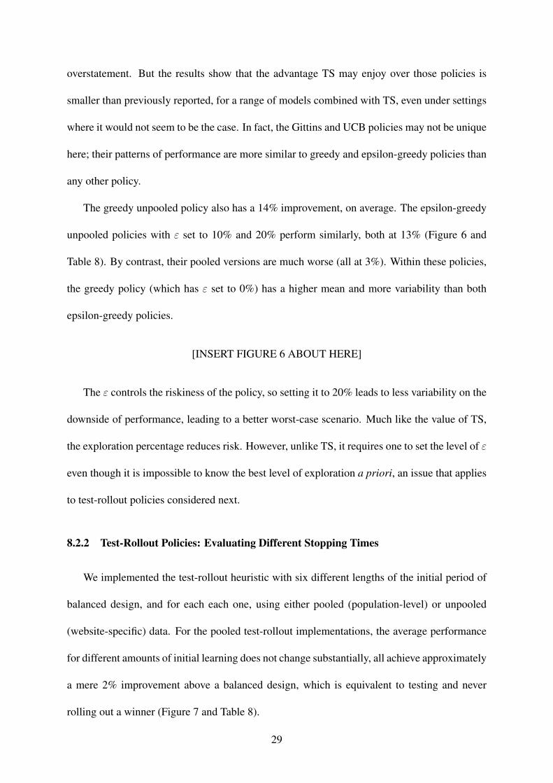
The greedy unpooled policy also has a 14% improvement, on average. The epsilon-greedy
unpooled policies with " set to 10% and 20% perform similarly, both at 13% (Figure 6 and
Table 8). By contrast, their pooled versions are much worse (all at 3%). Within these policies,
the greedy policy (which has " set to 0%) has a higher mean and more variability than both
epsilon-greedy policies.
[INSERT FIGURE 6 ABOUT HERE]
The " controls the riskiness of the policy, so setting it to 20% leads to less variability on the
downside of performance, leading to a better worst-case scenario. Much like the value of TS,
the exploration percentage reduces risk. However, unlike TS, it requires one to set the level of "
even though it is impossible to know the best level of exploration a priori, an issue that applies
to test-rollout policies considered next.
8.2.2 Test-Rollout Policies: Evaluating Different Stopping Times
We implemented the test-rollout heuristic with six different lengths of the initial period of
balanced design, and for each each one, using either pooled (population-level) or unpooled
(website-specific) data. For the pooled test-rollout implementations, the average performance
for different amounts of initial learning does not change substantially, all achieve approximately
a mere 2% improvement above a balanced design, which is equivalent to testing and never
rolling out a winner (Figure 7 and Table 8).
29

[INSERT FIGURE 7 ABOUT HERE]
The unpooled test-rollout policies perform much better than their pooled versions, and they
have a wider range of performance. The best average performance occurs when the balanced
experiment for every website-size combination lasts for 1 or 2 periods (both 10%) compared
to when it lasts for longer (between 7% and 9%). This simple policy can be surprisingly ef-
fective as it can beat the partially pooled policy, TS-HGLM, on average, and their performance
distributions overlap substantially.
These results may be somewhat idiosyncratic to the present setting. The impression volume
for period 1 included over 150 million impressions, approximately 20% of all observations,
which explains why there may have been enough information content, particularly for larger
volume websites, to learn the best ad from observed conversions alone. Nevertheless, the results
confirm that such a test-rollout policy is sensitive to the level of selecting a winner and the
choice of the test-period length, neither of which we would not know how to set in practice a
priori. In fact, setting test period length is precisely the optimal stopping problem underlying
bandit problems, as described in the introduction.
8.2.3 Discussion of Policy Counterfactuals
Our findings reveal the relative performance of each policy and which aspects of the meth-
ods are most important for improving performance. The list below collects the key findings,
which we support with evidence to follow:
• Model choice has more of an impact on policy performance than the choice of bandit
allocation rule.
• The partially pooled model with TS beats all pooled model policies.
30

• The unpooled policies beat their pooled versions, regardless of MAB allocation rule.
• The unpooled binomial model with TS and unpooled heuristic policies beat the partially
pooled model with TS.
• The partially pooled model has less variability than the unpooled binomial, among TS-
based policies.
While we may have thought that the choice of MAB allocation rule would be the most
important aspect of the policy, we find that the largest driver of policy performance is the
model choice: handling heterogeneity and the level of data aggregation – whether the model
is pooled, aggregating data across websites into a single population-level bandit problem, or
unpooled, treating each website’s bandit problem separately. Figure 8 presents the unpooled
version of each policy in order to highlight their relatively better performance and to show the
minor performance differences among them.
[INSERT FIGURE 8 ABOUT HERE]
Using a TS-based policy seems to be an attractive compromise, and even a partially pooled
TS policy layers an additional level of compromise. On one hand, the partially pooled approach
(TS-HGLM) always performs better than pooled policies. On the other hand, it does not beat
unpooled policies (including Gittins, UCB, epsilon-greedy, greedy, and test-rollout), on aver-
age, but it does have lower variability in performance than those unpooled policies. The lower
variability suggests it may be robust to changes in problem setting related to amount of data
per unit of observation.
The amount of data in each context is important. In this experiment, the Gittins, UCB,
unpooled greedy, epsilon-greedy, and test-rollout policies can outperform TS, but we note that
31

with enough data in each context, the partially pooled TS policy eventually approaches the
behavior of those unpooled policies.
9 Evaluating Sensitivity to Changes in Problem Setting
9.1 Changing the Timing of Updates, Batch Size, and Incidence Rate
While the preceding analyses evaluated different methods using these same true data gen-
erating process in the same setting, we now consider a counterfactual under a different setting.
What if we updated the allocations, wjkt, more frequently with smaller batch sizes, Mjt? What
if the conversion rates were different but still within random variation at the same order of mag-
nitude? This allows us to examine the robustness of the methods tested as well as investigate
boundary conditions of these MAB approaches.
The batching schedule in the actual experiment was weekly, so we re-ran the previously
discussed policies with daily updating instead of weekly updates, to show the impact of 62
batches instead of 10. We find the pattern of results for the policies we test is surprisingly robust
to using either weekly or daily batch sizes, with minimal to modest improvements using daily
instead of weekly updates. Our finding is consistent with the literature, but shows an attenuated
effect. TS performs better (and nearly similar to the Gittins index) for one-at-a-time updates
(batch size of 1 observation) (Scott 2010). Reducing each batch size has a slightly stronger
impact on the unpooled policies and winner-take-all policies, such as Greedy-unpooled (3%
improvement relative to the weekly batches), UCB-tuned-unpooled (3%), and Gittins-unpooled
(3%). Their corresponding pooled versions did not change. For TS-based policies, there was
less improvement for pooled (2%) and unpooled (1%). On the whole, however, decreasing
batch size improves performance, but not by much, for our dataset.
[INSERT TABLE 9 ABOUT HERE ]
32

9.2 Changing the Goal: Optimizing Clicks but Measuring Conversion
Often firms may run experiments and optimize those tests using easier to measure (or more
immediate) outcomes such as clicks instead of conversions as we used here. We re-ran the
analysis of various MAB policies using clicks as the outcome and highlight the difference
between optimizing clicks and conversions. We find that if you were to optimize click-through
rate, in hopes of having positive impact on downstream consequences such as conversions, you
would have an acquisition rate as bad as 12% worse than optimizing conversions directly.
This stems from the observation that the best ads for conversions are not the best for clicks.
The correlation is week (0.02, not significant) between click-through rate and conversion rate
across the 532 units of observation and is visible in the scatter plot contained in Figure 9. As
a result, optimizing for clicks, compared to optimizing for conversions, leads to very different
allocations.
[INSERT FIGURE 9 ABOUT HERE]
Before looking at the impact on conversions, we first examine how effective the policies
were in achieving their goal: aggregate click-through rate improvement. Since clicks occur
more frequently than conversions by multiple orders of magnitude (on average 4 clicks per
10,000 impressions), one imagines it is easier to optimize clicks. However, the relative effect
sizes between ads’ click through rates is even smaller than that for conversion rates. So there is
little systematic variation that the MAB policies can exploit to do much better than one another
for click-through rates.
As expected, all policies generate fewer conversions when optimizing for clicks, but the
size of the difference varies by policy. The policies most affected are those that perform better
when optimizing conversions (unpooled policies), and they suffer a loss between 8% to 12%.
TS attenuates this affect a bit with its variants suffering the least among unpooled policies (8%).
33

The pooled binomial (4%) and homogeneous logit (2%) are less affected. The policies nearly
unaffected are those that already do not perform well and are similar to a balanced policy.
More broadly, the differences between optimizing clicks versus conversions raises interesting
avenues of future research on consumer funnel that we discuss below.
10 General Discussion
We have intended to make two key contributions: we addressed a common problem in adap-
tive testing in online display advertising; and we drew upon a mix of disciplines to generalize
existing MAB problems in marketing. We have focused on improving the practice of real-time
adaptive experiments with online display advertisements to acquire customers. We translated
the components of the online advertiser’s problem into an MAB problem framework. The
component missing from existing MAB methods was a way to account for unobserved hetero-
geneity (e.g., ads differ in effectiveness when they appear on different websites) in the presence
of a hierarchical structure (e.g., ads within websites). We contribute this natural marriage of
hierarchical regression models and randomized allocation rules to the existing MAB policies.
We tested that policy in a live large-scale field experiment with a holdout control policy and
demonstrated it increased customer acquisition rate by 8% more than a balanced design.
However, we also show alternative MAB policies can reach similar and even better levels
of performance. By running counterfactual policy simulations, we find that the most influential
component of the MAB policies is the level of analysis: whether the policy is pooled or un-
pooled, due to significant website heterogeneity in conversion rates. Among unpooled policies,
even greedy, epsilon-greedy, and test-rollout policies perform as well as Gittins and UCB poli-
cies, all of which can perform modestly better than an unpooled or partially pooled TS policy,
in this setting. Nevertheless, due to the impact of both the TS rule and partial pooling, our
34

proposed policy controls variance of performance better than most of those alternatives, which
would be more susceptible to changes in setting, as in classic risk-reward trade-off.
The results can serve as a guide suggesting which policies are appropriate for different
settings. For instance, when consumer heterogeneity may be present, it should not be ignored.
It is even worth testing different parametric (partially pooled) and non-parametric (unpooled)
forms of heterogeneity. In addition, if it is possible to perform one-at-a-time updates, most
policies perform better. Index policies, such as Gittins and UCB policies, in particular, will
likely improve even more as they are applied at a more granular level, without batching and at
individual level.
Still there are limitations to our field experiment and simulations, which offer promising
future directions for research. We acknowledge that acquisition from a display ad is a complex
process, and we do not aim to capture all aspects of the acquisition funnel. We showed that
trying to optimize clicks leads to substantially worse conversion rates (Section 9.2).
Related to the consumer funnel, we do not explicitly address the effects of multiple expo-
sures within the campaign. But we acknowledge an individual may have seen more than one of
the ads during the experiment or the same ad multiple times. The issue of multiple campaign
exposures would raise concerns if the following conditions were true: (i) the repeated viewing
of particular types of ads has a substantially different impact on acquisition than the repeated
viewing of other types of ads; (ii) that difference is so large that a model including accounting
for repeated exposures would identify different winning ads than a model that ignores them;
and (iii) there is a difference in the identified winning ad for many of the websites with large
impression volume. While this scenario is possible, we believe it is unlikely. An additional
assumption that would be problematic more generally is the assumed stationarity of conversion
rates at the website-ad level. The data suggest the assumption of a constant µjk is reasonable
35
during our experiment, and most of the variation in aggregate conversion rates, viewed in Fig-
ure 3 can be attributed to changes in the mix of impression volume across media placements
outside of our decision-making control.
Ignoring the consumer funnel was a constraint in our data and setting. Due to the scale of
the campaign the advertiser did not collect individual-level or cookie-level panel data. Indeed
advertisers often only work at the level of media placement, ad, and time period, instead of
individual customers over time. Working with that individual data with repeated ad exposures,
however, would offer an opportunity to combine research in MAB problems with ad attribution
modeling (Braun and Moe 2013). To focus on repeated interactions with the same individ-
ual could also suggest an entirely different framework: dynamic treatment regimes, used in a
stream of clinical trials (Murphy 2005).
A second limitation is that we do not take into account the known finite-time horizon or the
potential size of the population affected by the decisions after the experiment. If the relative
cost required to run the experiment is negligible, then there is little benefit from optimizing the
experiment during that period. This reduces to a test-rollout setting where it is best to learn
then earn. By contrast, if the observations are relatively costly or if there is always earning to
be gained from learning, then it would be useful to consider a MAB experiment for an infinite
horizon. However, most MAB experiments fall somewhere between those two extremes. The
length of the MAB experiment is a decision that the experimenter should optimize and is the
subject of two streams of research. A family of methods known as expected value of informa-
tion gained and knowledge gradient optimize this extra optimal stopping problem in a bandit
setting (Chick and Gans 2009; Chick and Inoue 2001; Chick et al. 2010; Frazier et al. 2009;
Powell 2011). The other stream of research is known as patient horizon, explicitly considering
the relative number of patients in clinical trials and potential patient population affected by the
36

conclusions (Berry 1972, 2004). Both have promise for improving A/B testing practices and
research in marketing involving experiments and bandit problems.
Third, future research may aim to generalize our problem to a setting of media buying
and planning in which we had control of the batch size and allocate impression volume across
websites with varying media costs. Our analysis applied to a mix of media purchased via cost-
per-impression, cost-per-click, and cost-per-action since the budget was allocated in advance
for each media placement regardless of method of purchase. We treated batch size as exogenous
for each website and each period. Instead, however, future research could account for the
complex interplay among impression volume, type of media buy, cost per impression, and
expected conversion rate. This is relevant as real-time bidding for media on ad exchanges and
automated media buying such as programmatic advertising become even more common.
Finally, we consider another limitation in our data: we only observe conversion without
linking those customers to their subsequent behavior. It seems natural to acquire customers by
considering the relative values of their expected customer lifetime value (CLV) and cost per
acquisition (CPA) instead of merely seeking to increase acquisition rate (i.e., lower cost per
acquisition). Improving CPA alone is important since it guides future budget decisions, e.g.,
willingness to spend for each expected acquisition; however, sequentially allocating resources
to acquire customers based on predictions about their future return on acquisition investment
(CLV/CPA) seems like a promising marriage between MAB and CLV literature.
We see the MAB problem as a powerful framework for optimizing a wide range of business
operations. As we continue equipping managers and marketing researchers with these tools to
employ in a wide range of settings, we should have a more systematic understanding of the
robustness and sensitivity of these methods to common practical issues.
37

References
Agarwal, Deepak, Bee-Chung Chen, Pradheep Elango. 2008. Explore/Exploit Schemes forWeb Content Optimization. Yahoo Research paper series .
Agrawal, Rajeev. 1995. Sample Mean Based Index Policies with O(log n) Regret for the Multi-Armed Bandit Problem. Advances in Applied Probability 27(4) 1054–1078.
Agrawal, Shipra, Navin Goyal. 2012. Analysis of Thompson Sampling for the multi-armedbandit problem. Journal of Machine Learning Research Conference Proceedings, Confer-
ence on Learning Theory 23(39) 1–26.
Anderson, Eric, Duncan Simester. 2011. A Step-by-Step Guide to Smart Business Experiments.Harvard Business Review 89(3) 98–105.
Auer, Peter. 2002. Using Confidence Bounds for Exploitation-Exploration Trade-offs. Journal
of Machine Learning Research (3) 397–422.
Bates, Douglas, Martin Maechler, Ben Bolker, Steven Walker. 2013. R Package ’lme4’Http://cran.r-project.org/web/packages/lme4/lme4.pdf.
Bates, Douglas, Donald G. Watts. 1988. Nonlinear Regression Analysis and Its Applications.Wiley.
Berry, Donald A. 1972. A Bernoulli Two-Armed Bandit. Annals of Mathematical Statistics 43871–897.
Berry, Donald A. 2004. Bayesian Statistics and the Efficiency and Ethics of Clinical Trials.Statistical Science 19(1) 175–187.
Berry, Donald A., Bert Fristedt. 1985. Bandit Problems. Chapman Hall.
Bertsimas, Dimitris, Adam J. Mersereau. 2007. Learning Approach for Interactive Marketing.Operations Research 55(6) 1120–1135.
Bradt, R. N., S. M. Johnson, S. Karlin. 1956. On Sequential Designs for Maximizing the Sumof n Observations. Annals of Mathematical Statistics 27(4) 1060–1074.
Braun, Michael, Wendy W. Moe. 2013. Online Display Advertising: Modeling the Effects ofMultiple Creatives and Individual Impression Histories. Marketing Science 32(5) 753–767.
Brezzi, M., T. L. Lai. 2002. Optimal Learning and Experimentation in Bandit Problems. Jour-
nal of Economic Dynamics and Control 27 87–108.
Chapelle, Olivier, Lihong Li. 2011. An Empirical Evaluation of Thompson Sampling. Online
Trading of Exploration and Exploitation workshop 1–6.
Chick, S. E., P. Frazier. 2012. Sequential Sampling with Economics of Selection Procedures.Management Science 58(3) 550–569.
Chick, S.E., N. Gans. 2009. Economic analysis of simulation selection problems. Management
Science 55(3) 421–437.
38

Chick, S.E., K. Inoue. 2001. New Two-Stage and Sequential Procedures for Selecting the BestSimulated System. Operations Research 49(5) 732–743.
Chick, S.E., Branke J., Schmidt C. 2010. Sequential Sampling to Myopically Maximize theExpected Value of Information. INFORMS Journal on Computing 22(1) 71–80.
Dani, V., T. P. Hayes, S. M. Kakade. 2008. Stochastic Linear Optimization Under BanditFeedback. Conference on Learning Theory .
Davenport, Thomas H. 2009. How to Design Smart Business Experiments. Harvard Business
Review 87(2) 1–9.
Donahoe, John. 2011. How ebay Developed a Culture of Experimentation: HBR Interview ofJohn Donahoe. Havard Business Review 89(3) 92–97.
Filippi, Sarah, Olivier Cappe, Aurelien Garivier, Csaba Szepesvari. 2010. Parametric bandits:The generalized linear case. J. Lafferty, C. K. I. Williams, J. Shawe-Taylor, R.S. Zemel,A. Culotta, eds., Advances in Neural Information Processing Systems 23. 586–594.
Frazier, P.I., W.B. Powell, S. Dayanik. 2009. The Knowledge-Gradient Policy for CorrelatedNormal Beliefs. INFORMS Journal on Computing 21(4) 599–613.
Gelman, Andrew, John B. Carlin, Hal S. Stern, Donald B. Rubin. 2004. Bayesian Data Analy-
sis. 2nd ed. Chapman & Hall, New York, NY.
Gelman, Andrew, Jennifer Hill. 2007. Data Analysis Using Regression and Multi-
level/Hierarchical Models. Cambridge University Press, New York, NY.
Gittins, John C. 1979. Bandit Processes and Dynamic Allocation Indices. Journal of the Royal
Statistical Society, Series B 41(2) 148–177.
Gittins, John C., Kevin Glazebrook, Richard Weber. 2011. Multi-Armed Bandit Allocation
Indices. 2nd ed. John Wiley and Sons, New York, NY.
Goldfarb, Avi, Catherine Tucker. 2011. Online Display Advertising: Targeting and Obtrusive-ness. Marketing Science 30(3) 389–404.
Granmo, O.-C. 2010. Solving Two-Armed Bernoulli Bandit Problems Using a Bayesian Learn-ing Automaton. International Journal of Intelligent Computing and Cybernetics 3(2) 207–232.
Hauser, John R., Guilherme Liberali, Glen L. Urban. 2014. Website Morphing 2.0: Technicaland Implementation Advances and a Field Experiment. Management Science 60(6) 1594–1616.
Hauser, John R., Glen L. Urban, Guilherme Liberali, Michael Braun. 2009. Website Morphing.Marketing Science 28(2) 202–223.
Hoban, Paul, Randy Bucklin. 2015. TITLE. Journal of Marketing Research 40(1) 1–19.
Kaufmann, Emilie, Nathaniel Korda, Remi Munos. 2012. Thompson Sampling: An Asymp-totically Optimal Finite Time Analysis http://arxiv.org/abs/1205.4217/.
39

Keller, Godfrey, Alison Oldale. 2003. Branching Bandits: A Sequential Search Process withCorrelated Pay-offs. Journal of Economic Theory 113(2) 302–315.
Krishnamurthy, V., Bo Wahlberg. 2009. Partially Observed Markov Decision Process Multi-armed Bandits: Structural Results. Mathematics of Operations Research 34(2) 287–302.
Lai, T. L. 1987. Adaptive Treatment Allocation and the Multi-Armed Bandit Problem. Annals
of Statistics 15(3) 1091–1114.
Lambrecht, Anja, Catherine Tucker. 2013. When Does Retargeting Work? Information Speci-ficity in Online Advertising. Journal of Marketing Research 50(5) 561–576.
Lin, Song, Juanjuan Zhang, John Hauser. 2015. Learning from Experience, Simply. Marketing
Science 34(1) 1–19.
Manchanda, Puneet, Jean-Pierre Dube, K.Y. Goh, P.K. Chintagunta. 2006. The Effect of BannerAdvertising on Internet Purchasing. Journal of Marketing Research 43(February) 98–108.
May, Benedict C., Nathan Korda, Anthony Lee, David S. Leslie. 2011. Optimistic BayesianSampling in Contextual Bandit Problems. Department of Mathematics, University of Bristol
(Technical Report 11:01).
Meyer, Robert J., Y. Shi. 1995. Sequential Choice Under Ambiguity: Intuitive Solutions to theArmed-Bandit Problem. Management Science 41(5) 817–834.
Murphy, Susan A. 2005. An experimental design for the development of adaptive treatmentstrategies. Statistics in Medicine 24 1455–1481.
Ortega, Pedro A., Daniel A. Braun. 2010. A Minimum Relative Entropy Principle for Learningand Acting. Journal of Artificial Intelligence Research 38 475–511.
Ortega, Pedro A., Daniel A. Braun. 2013. Generalized Thompson Sampling for SequentialDecision-Making and Causal Inference http://arxiv.org/abs/1303.4431.
Osband, Ian, Daniel Russo, Benjamin VanRoy. 2013. (More) Efficient Reinforcement Learningvia Posterior Sampling http://arxiv.org/abs/1306.0940.
Perchet, Vianney, Philippe Rigollet, Sylvain Chassang, Erik Snowberg. 2015. Batched BanditProblems. Arxiv (1505.00369). Http://arxiv.org/abs/1505.00369.
Powell, Warren B. 2011. Approximate Dynamic Programming: Solving the Curses of Dimen-
sionality. Wiley, New Jersey.
Reiley, David, Randall Aaron Lewis, Panagiotis Papadimitriou, Hector Garcia-Molina, Prab-hakar Krishnamurthy. 2011. Display Advertising Impact: Search Lift and Social Influence.Proceedings of the 17th ACM SIGKDD Conference on Knowledge Discovery and Data Min-
ing. 1019–1027.
Robbins, H. 1952. Some Aspects of the Sequential Design of Experiments. Bulletin of the
American Mathematics Society 58(5) 527–535.
Rubin, Donald. 1990. Estimating Causal Effects of Treatments in Randomized and Nonran-domized Studies. Journal of Educational Psychology 66(5) 688–701.
40

Rusmevichientong, Paat, John N. Tsitsiklis. 2010. Linearly Parameterized Bandits. Mathemat-
ics of Operations Research 35(2) 395–411.
Russo, Daniel, Benjamin VanRoy. 2014. Learning to Optimize Via Posterior Sampling. Math-
ematics of Operations Research 39(4) 1221–1243.
Scott, Steven L. 2010. A Modern Bayesian Look at the Multi-Armed Bandit. Applied Stochastic
Models Business and Industry 26(6) 639–658.
Sutton, Richard S., Andrew G. Barto. 1998. Reinforcement Learning: An Introduction. MITPress, Cambridge, MA.
Thompson, Walter R. 1933. On the Likelihood that One Unknown Probability Exceeds Anotherin View of the Evidence of Two Samples. Biometrika 25(3) 285–294.
Tsitsiklis, John N. 1986. A Lemma on the Multi-Armed Bandit Problem. IEEE Transactions
on Automatic Control 31(6) 576–577.
Urban, Glen L., Guilherme Liberali, Robert Bordley, Erin MacDonald, John R. Hauser. 2014.Morphing Banner Advertising. Marketing Science 33(1) 27–46.
Wahrenberger, David L., Charles E. Antle, Lawarence A. Klimko. 1977. Bayesian Rules forthe Two-armed Bandit Problem. Biometrika 64(1) 1724.
White, John Myles. 2012. Bandit Algorithms for Website Optimization. O’Reilly Media.
Whittle, P. 1980. Multi-armed Bandits and the Gittins Index. Journal of Royal Statistical
Society, Series B 42(2) 143–149.
41

Appendix
We examine how the TS-HGLM policy works by focusing on the three aspects of the policy:
(1) how allocations differ across combinations of ad concept and ad size (i.e., attributes), (2)
how allocations differ across websites (i.e., heterogeneity), and (3) how allocations across ads
within a website change over time (i.e., learning). Consider two representative websites (j =
103 and 149) highlighted at two time points (t = 1 and 6) in Figure 10. The boxplots and
lines summarize the predictive marginal distributions of the corresponding µjk(✓) based on the
HGLM.
[INSERT FIGURE 10 ABOUT HERE]
[INSERT TABLES 10, 11, AND 12 ABOUT HERE]
We see ad attribute importance by noting the differences in the µjk(✓) distributions across
the ad concepts and ad sizes (within a website at any snapshot in time). In particular, it is clear
that the interactions between ad concepts and ad sizes are meaningful: the rank order of the ad
concepts’ conversion rates varies for different ad sizes. For instance, consider the snapshot of
how the TS-HGLM policy evaluated ads and allocated impressions to website j = 103 using
data through t = 6. This is shown as the second row (from the top) of four panels in Figure
10, which we continue to refer to throughout this subsection to explain the findings about ad
attributes. For ad size A, the ad concept with the best predicted mean conversion rate is ad
concept 4 (14 acquisitions per million impressions), but that same concept is neither the best
on the ad size B (mean conversion rate is 131 per million) nor on C (mean conversion rate is
47 per million). In both cases, the best predicted ad concept for sizes B and C is ad concept 3.
The distributions of µjk(✓) shown as boxplots in Figure 10 are the heart of the TS proce-
dure. They represent our current beliefs in the conversion rates reflecting our uncertainty in the
42

HGLM parameters based on the data through t periods. At the end of each period, we simulate
G draws from each of those distributions. Using these empirical distributions, we approximate
the probability that each ad has the highest mean for each website-by-size pair.
As a result of this procedure, the right side of each panel of Figure 10 shows the next set
of allocation probabilities, wj,k,t+1
, within each ad size, website, and time period for all ad
concepts. Looking at these allocation probabilities for j = 103 using data through t = 6, we
see that for sizes B and C, ad concept 1 is hardly given any impressions in the next period.
However, for size A, ad concept 1 is actually predicted to be as good as ad concept 3.
Figure 10 not only shows the importance of attributes (differences within a website across
ads), but it also shows learning (changes within an ad-website combination over time) and
heterogeneity (differences across websites). The MAB policy learns parameters over time. In
our case, it is not practical to report how all parameters are learned, but we highlight how the
TS-HGLM policy updates its beliefs about µjk(✓) for particular ad-website combinations. It is
clear from Figure 10 that the distributions are wider after the initial period (t = 1) than they are
after more data has accumulated (t = 6).
For instance, after the initial period (t = 1) for ad size B and ad concept 3, the predicted
distribution of the conversion rate has a 95% interval of (0.92, 56.65) with a mean of 7.35 per
million. The probability that it is optimal is 27%. Later on, after the policy learns more about
the parameters (t = 6), we see that the interval not only shrinks (0.82, 10.31), but also shifts its
mean to 2.93 customers per million impressions. This leads the MAB policy to assign a higher
probability that this ad concept is optimal, hence allocating 41% of impressions for the next
period.
The unobserved heterogeneity in the hierarchical model leads allocations to differ across
websites. For example, the two websites in Figure 10 have different winning ads. After t = 6
43

periods, for website j = 103, the predicted winners for each ad size (A, B, and C) are ad
concepts 4, 3, and 3, whereas those for website j = 149 are ad concepts 1, 3, and 4, respectively.
Capturing such patterns of website-to-website differences enables the proposed MAB policy to
reach greater improvement than other MAB policies that may ignore those patterns.
The key benefit of partial pooling is capturing heterogeneity across websites, but an added
benefit is providing a predictive distribution for the ads on any website in question, even in the
absence of a large amount of data on that website. Such sparse data on any one website is a nat-
ural feature of this problem. If we were to rely on the observed data alone, especially early in
the experiment, we would see that observed conversion rates would be highly misleading. After
the initial period for website j = 149, there were zero conversions in total, except for some
customer acquisition from ad concept 2 on ad size B. That would be rated the best ad concept
and ad size combination if we were only using the observed conversion rate for evaluating the
ads. But can we really trust that signal given the rare incidence rate in the environment? Trust-
ing that data alone, without leveraging other information, would be problematic; typically, such
oversight leads to significant variability in performance of any policy that relies heavily on ob-
served data (e.g., policies referred to as greedy) and independently on each unit’s observations
(e.g., policies that lack partial pooling across websites).
Tables 10, 11, and 12 provide the underlying key values illustrated in the panels of Figure
10 (one table for each ad size), as well as the observed data of cumulative conversions and
impressions broken down by two time periods (t = 1 and 6), two websites (j = 103 and
149), each ad size (A, B, and C), and each ad concept (1, 2, 3, and 4). The belief distributions
of µjk(✓) for all k and the two j are summarized by mean and 95% intervals. The resulting
allocations, wj,k,t+1
, are shown in the tables and match those shown in Figure 10.
44

11 Tables and Figures
Publishers
About.comAllRecipes.comAOL IncAT&T.comBBCCars.comCNNCurrent TVEducation.comFederated MediaGoogleGoogle Display ReserveHooklogic.comMeredith CorporationMSNNBC UniversalNew York MagazinePhilly.comSalon.comScripps NetworkSynacorTime IncTurner BroadcastingWhite PagesX plus 1YahooYelp.com
Table 1: List of online media publishers. The display ad campaign involved all of these pub-lishers.
45

Category Impressions Clicks Conversions Observations per period
Contextual 16,947,970 23,424 162 28Demand-side platform 169,904,767 69,675 288 72
Lifestyle site 37,045,487 7,283 216 28News site 85,423,919 42,188 200 112
Personal finance 290,437 169 6 8Portal 319,747,702 150,857 688 120
Reference Directory 25,447,441 3,523 72 20Retargeting 101,766,713 39,502 1,730 144
Total 756,574,436 336,621 3,362 532
Table 2: Categories of media placements. The table summarizes the data by the media cate-gories and types of advertisement methods used in the field experiment over all 62 days.
46

Pearson correlation
1 2 3 41 1 0.843 0.646 0.8472 0.843 1 0.743 0.8903 0.646 0.743 1 0.7394 0.847 0.890 0.739 1
Spearman rank-order correlation
1 2 3 4
1 1 0.657 0.526 0.6492 0.657 1 0.542 0.6603 0.526 0.542 1 0.6424 0.649 0.660 0.642 1
Table 3: Correlation of ad concept conversion rates across media placements. Pearson andSpearman rank-order correlation matrices show that conversion rates covary, across 133 uniquewebsite-ad-size combinations, but their rank ordering is less consistent than their magnitudes.
47

Balanced policy: wkt =1
K
for all t
Test-rollout(⌧) Pooled: ˆkt = argmaxk {µk} wkt =
8
>
<
>
:
1K , for t ⌧
(
1, for k =
ˆ
kt, t > ⌧
0, otherwise, t > ⌧
Test-rollout(⌧) Unpooled: ˆkjt = argmaxk {µjk} wjkt =
8
>
<
>
:
1K , for t ⌧
(
1, for k =
ˆ
kjt, t > ⌧
0, otherwise, t > ⌧
Greedy Pooled: ˆkt = argmaxk {µk} wkt =
(
1, for k =
ˆ
kt
0, otherwise
Greedy Unpooled: ˆkjt = argmaxk {µjk} wjkt =
(
1, for k =
ˆ
kjt
0, otherwise
Epsilon-greedy(") Pooled: ˆkt = argmaxk {µk} wkt =
(
(1� ") +
"K , for k =
ˆ
kt,
"K , otherwise
Epsilon-greedy(") Unpooled: ˆkjt = argmaxk {µjk} wjkt =
(
(1� ") +
"K , for k =
ˆ
kjt,
"K , otherwise
UCB1 Pooled: ˆkt = argmaxk
(
µkt +
r
2 logMt
mkt
)
wkt =
(
1, for k =
ˆ
kt
0, otherwise
UCB1 Unpooled: ˆkjt = argmaxk
(
µjkt +
s
2 logMjt
mjkt
)
wjkt =
(
1, for k =
ˆ
kjt
0, otherwise
UCB-Tuned Pooled: ˆkt = argmaxk
(
µkt +
s
logMt
mktmin
⇢
1
4
, Vkt
�
)
wkt =
(
1, for k =
ˆ
kt
0, otherwise
where Vkt = �
2kt +
r
2 logMt
mkt, and we observe �
2kt,Mt,mkt
UCB-Tuned Unpooled: ˆkjt = argmaxk
(
µjkt +
s
logMjt
mjktmin
⇢
1
4
, Vjkt
�
)
wkt =
(
1, for k =
ˆ
kt
0, otherwise
where Vjkt = �
2jkt +
s
2 logMjt
mjkt, and we observe �
2jkt,Mjt,mjkt
Table 4: MAB policies using heuristics and upper confidence bound (UCB). “Pooled”refers to a policy or model where data are aggregated across all websites and alloca-tions are the same across all websites. “Unpooled” refers to a policy or model wheredata are separated by each website and allocations are website-specific. Pooled observedmean is µk =
PJj=1
Pt�1
s=1
yjks/PJ
j=1
Pt�1
s=1
mjks. The unpooled observed mean is µjk =
Pt�1
s=1
yjks/Pt�1
s=1
mjks
48

Gittins Pooled: ˆkt = argmaxk {G(akt, bkt, �)} wkt =
(
1, for k =
ˆ
kt
0, otherwise
where akt = ak0 +
JX
j=1
t�1X
s=1
yjks, and bkt = bk0 +
JX
j=1
t�1X
s=1
(mjks � yjks)
Gittins Unpooled: ˆkjt = argmaxk {Gjkt(ajkt, bjkt, �)} wjkt =
(
1, for k =
ˆ
kjt
0, otherwise
where ajkt = ajk0 +
t�1X
s=1
yjks, and bjkt = bjk0 +
t�1X
s=1
(mjks � yjks)
TS with binomial model and beta prior distribution
TS-BB-pooled: wkt =
Z
µ1 {µk = µ⇤|µ} p(µ|yt�1,mt�1)dµ
p(µk|yt�1,mt�1) = beta(akt, bkt), for each k
akt = ak0 +
JX
j=1
t�1X
s=1
yjks, and bkt = bk0 +
JX
j=1
t�1X
s=1
(mjks � yjks)
TS-BB-unpooled: wjkt =
Z
µj
1 {µjk = µj⇤|µj} p(µj |yj,t�1,mj,t�1)dµj
p(µjk|yj,t�1,mj,t�1) = beta(ajkt, bjkt), for each j, k
ajkt = ajk0 +
t�1X
s=1
yjks, and bjkt = bjk0 +
t�1X
s=1
(mjks � yjks)
TS with a homogeneous generalized linear model (pooled)
TS-GLM: wkt =
Z
�1⇢
¯
�xk = max
k¯
�xk|¯�, X�
p(
¯
�|yt,mt)d¯
�
ykt ⇠ binomial (µk|mkt)
µk = 1/
⇥
1 + exp(�x
0k¯
�)
⇤
TS with a latent-class generalized linear model
TS-LCGLM: wkt =
Z
�1
Z
�2
Z
⇡
Z
z21,21⇢
�zjxk = max
k�zjxk|z,�zj , X
�
p(�1,�2,⇡, z|yt,mt)dzd⇡d�1d�2
yjkt|zj ⇠ binomial (µjk|mjkt)
µjk|zj = 1/ [1 + exp(�x
0k�j)]
zj |⇡ ⇠ multinomial(⇡1,⇡2), ⇡1 + ⇡2 = 1, and �j 2 {�1,�2}
TS with a hierarchical generalized linear model (partial pooling)
TS-HGLM: wjkt =
Z
⌃
Z
�
Z
�1,...,�J
1⇢
�jxk = max
k�jxk|�j , X
�
p(�j |¯�,⌃, X,yt,mt)p(¯
�,⌃|�1, . . . ,�J)d�1 . . . d�Jd¯
�d⌃
yjkt ⇠ binomial (µjk|mjkt)
µjk = 1/ [1 + exp(�x
0k�j)]
�j ⇠ N(
¯
�,⌃)
Table 5: MAB policies using Gittins index and Thompson Sampling (TS).
49

Period Impressions
1 151,404,4792 78,201,8893 78,263,7524 33,864,6495 53,628,3006 79,520,6907 73,238,4488 104,740,9329 59,557,343
10 44,153,954
Total 756,574,436
Table 6: Impression volume. Impression volumes were predetermined per period and outsideof our experimental control. We randomly split 80% and 20% of impressions into the treat-ment and control groups, respectively. Each period the Treatment policy involved changing adallocation.
50

Ad Size Ad Concept Impressions Clicks Conversions Conversion rate Observations
A1 55,214,371 26,875 287 5.20 392 29,989,021 15,635 131 4.37 393 42,180,270 20,874 203 4.81 394 48,426,287 29,981 359 7.41 39
B1 81,677,801 32,337 390 4.77 502 87,119,895 34,176 299 3.43 503 52,631,340 22,764 319 6.06 504 69,864,609 31,599 348 4.98 50
C1 46,826,804 18,575 229 4.89 442 52,164,963 20,741 215 4.12 443 77,066,851 31,930 219 2.84 444 113,412,224 51,134 363 3.20 44
Total 756,574,436 336,621 3,362 4.44 532
Table 7: Aggregate summary statistics. The table summarizes impressions, clicks, and conver-sions combined from the test and control groups, split by the 12 ads in the field experimentafter 62 days. The observations represents the number of units of observation used per period,which are unique website-size-concept combinations. Conversion rate is number of customersacquired per million impressions.
51

Policy Bandit allocation Model Relative mean Mean SD 2.5% 97.5%
Balanced Pooled 0% 4.373 0.138 4.052 4.569
Test-rollout 1 Pooled 2% 4.453 0.155 4.157 4.721Test-rollout 2 Pooled 2% 4.479 0.128 4.194 4.700Test-rollout 3 Pooled 2% 4.463 0.108 4.243 4.631Test-rollout 4 Pooled 2% 4.463 0.099 4.242 4.610Test-rollout 5 Pooled 2% 4.446 0.098 4.216 4.591Test-rollout 6 Pooled 2% 4.450 0.085 4.284 4.610
Test-rollout 1 Unpooled 10% 4.814 0.118 4.593 5.030Test-rollout 2 Unpooled 10% 4.822 0.100 4.617 5.009Test-rollout 3 Unpooled 9% 4.778 0.094 4.588 4.941Test-rollout 4 Unpooled 9% 4.751 0.093 4.588 4.941Test-rollout 5 Unpooled 8% 4.707 0.088 4.557 4.891Test-rollout 6 Unpooled 7% 4.668 0.088 4.469 4.832
Greedy Pooled 3% 4.520 0.115 4.274 4.726Greedy Unpooled 14% 4.992 0.117 4.799 5.198Epsilon-greedy(10) Pooled 3% 4.489 0.094 4.276 4.654Epsilon-greedy(20) Pooled 3% 4.504 0.089 4.348 4.663Epsilon-greedy(10) Unpooled 13% 4.951 0.086 4.754 5.088Epsilon-greedy(20) Unpooled 13% 4.957 0.094 4.784 5.127
Gittins Pooled 3% 4.513 0.112 4.278 4.705Gittins Unpooled 13% 4.954 0.086 4.807 5.097UCB1 Unpooled 0% 4.366 0.072 4.192 4.493UCB-tuned Unpooled 14% 5.005 0.103 4.789 5.190
TS-binomial-pooled Thomspon Pooled binomial 3% 4.493 0.087 4.340 4.666TS-binomial-unpooled Thomspon Unpooled binomial 10% 4.832 0.102 4.619 5.024TS-GLM Thomspon Pooled logit 3% 4.493 0.091 4.334 4.662TS-LCGLM Thomspon Latent-class logit 4% 4.527 0.088 4.353 4.682TS-HGLM Thomspon Partially pooled logit 8% 4.717 0.090 4.560 4.900
Perfect information 36% 5.932 0.078 5.785 6.080
Table 8: Summary of performance for all MAB policies tested. The mean, standard deviation,and percentiles summarize the distribution of performance from the 100 simulated replicates ofeach policy. The relative mean is defined as a percentage better than the Balanced experiment.The better performing policies appear in bold.
52

Daily batches ImprovementPolicy Mean SD (Daily / Weekly)
Balanced 4.333 0.099 -0.9%Epsilon-greedy(10) Pooled 4.547 0.068 1.3%Epsilon-greedy(20) Pooled 4.490 0.012 -0.3%Epsilon-greedy(10) Unooled 4.972 0.115 0.4%Epsilon-greedy(20) Unpooled 4.975 0.071 0.4%Greedy Pooled 4.543 0.103 0.5%Greedy Unpooled 5.124 0.060 2.6%Gittins Pooled 4.516 0.065 0.1%Gittins Unpooled 5.059 0.114 2.1%UCB1 unpooled 4.348 0.057 -0.4%UCB-tuned unpooled 5.112 0.120 2.1%TS-BB-pooled 4.576 0.067 1.8%TS-BB-unpooled 4.891 0.076 1.2%Perfect information 5.942 0.094 0.2%
Table 9: Improvement from daily instead of weekly batching. Daily batching improves meanperformance compared to weekly batching for nearly all policies. The percent improvement isbased on the mean in this table for daily batching and the mean from the previous table showingweekly batching. The mean and standard deviation summarize the distribution of performancefrom the 100 simulated replicates of the selection of policies considered.
53

size A
website time concept wj,k,t+1 µjk Mean µjk 2.5% µjk 97.5% yjkt mjkt
j103 1 1 0.30 4.76 0.42 43.70 0 130862 0.27 3.99 0.36 46.47 0 130863 0.19 2.81 0.19 40.03 0 130864 0.23 3.64 0.25 43.96 0 13086
6 1 0.24 12.99 4.52 35.13 1 964152 0.17 9.94 2.71 36.93 1 787763 0.26 12.73 3.84 44.13 1 865404 0.33 13.88 4.23 41.37 2 97296
j149 1 1 0.27 5.83 0.55 64.33 0 35722 0.25 4.84 0.34 64.83 0 35723 0.22 3.99 0.19 79.68 0 35724 0.27 4.70 0.29 85.16 0 3572
6 1 0.30 6.08 1.09 33.82 1 480282 0.16 3.43 0.47 22.71 0 389143 0.28 5.61 0.82 37.47 0 402814 0.27 5.05 0.66 37.00 0 48360
Table 10: Values from Figure 10 for ad size A. The predictive distribution of each µjk based onthe model and data through t periods, is summarized by its mean (column labeled “µjk Mean”)and 95% interval (columns labeled µjk 2.5% and µjk 97.5%). The predictive distributions arebased on the actual cumulative number of conversions and impressions (columns labeled yjkt
and mjkt, respectively). The subsequent allocation weights are for period t+1 (column labeledwj,k,t+1
). The above descriptions apply here and to Tables 11 and 12.
54

size B
website time concept wj,k,t+1 µjk Mean µjk 2.5% µjk 97.5% yjkt mjkt
j103 1 1 0.01 76.05 28.40 210.40 1 182152 0.22 165.29 56.90 492.54 5 182153 0.41 210.07 78.38 662.32 5 182154 0.37 206.97 75.22 554.49 3 18215
6 1 0.01 88.70 44.36 171.69 2 248142 0.30 147.29 71.24 303.86 14 888263 0.52 167.57 89.55 299.38 36 2072584 0.18 131.02 61.53 294.88 8 61298
j149 1 1 0.16 5.69 1.07 36.85 0 283562 0.33 9.03 1.41 63.44 1 283563 0.27 7.35 0.92 56.65 0 283564 0.23 6.81 1.03 56.76 0 28356
6 1 0.21 2.35 0.76 7.41 0 2951322 0.22 2.17 0.59 8.67 1 4043843 0.41 2.93 0.82 10.31 2 4034674 0.15 1.87 0.52 7.18 0 302950
Table 11: Values from Figure 10 for ad size B.
55

size C
website time concept wj,k,t+1 µjk Mean µjk 2.5% µjk 97.5% yjkt mjkt
j103 1 1 0.10 27.48 6.68 116.32 2 174392 0.08 21.36 4.27 93.26 1 174393 0.26 40.23 8.58 190.65 0 174394 0.57 61.37 14.87 256.00 1 17439
6 1 0.02 26.28 12.08 58.81 3 433232 0.31 45.15 17.26 119.30 4 407873 0.39 50.49 20.97 121.70 5 1024414 0.28 47.01 19.73 111.75 3 115023
j149 1 1 0.23 3.31 0.29 31.32 0 140592 0.18 2.78 0.29 31.35 0 140593 0.22 2.98 0.20 42.94 0 140594 0.37 5.01 0.50 75.27 0 14059
6 1 0.25 1.63 0.36 6.97 0 1863822 0.20 1.34 0.23 8.13 0 1579233 0.22 1.53 0.32 6.60 0 2225764 0.33 1.90 0.33 9.14 1 288744
Table 12: Values from Figure 10 for ad size C.
56

Rates less than 1/100,000
Obs. conversion rate
Freq
uenc
y
0e+00 4e−06 8e−06
050
100
150
200
Rates greater than 1/100,000
Obs. conversion rate
0.00000 0.00010 0.00020
010
2030
4050
Figure 1: Histogram of conversion rates. Each observation is the number of conversions perimpression over 62 days of the field experiment for one of the 532 unique website-size-conceptcombinations.
57

●●
●●
●
●
●●●
●●● ●
●
●
●
●
●
●
●
●
●
●●●
●●●
●
●●
●●
●
●
●
●
●
●
●
●
●
●
●
●●
●
●
●
●
●●
●
●
●
●
●
●
●●
●
●●
●
●
●
●
●
●
●
●
●
●
●
●
●
●
●
●
●
●
●
●
●
●
●
●●
●●
●
●
●
●●
●
●●
●●
●
●
● ●
●
●
●
●
●●●
●●
●
●
●●● ●●
●
●●
●
●
●
●
●
●
●
●
●
●
●●●
●
●●
●
●
●
●
●
●
●●
●
●●
●●
●
●
●●
●
●
●
●
●
●
●
●●
●●
●
●
●
●
●
●
●
●
●
●●
●●
●●
●
●
●
●
●
●
●●
●
●●
●
●●●
●
●
●●
●
●●
●
● ●
●
●●
●●
●
●
●
●
●
●●
●
●
●
●
●
●
●
●
●
●
●
●
●
●
●●
●
●
●●
●
●
●●
●●
●
●
●●●
●
●
●
●
●
●
●
●
●
●●
●●
●
●●●
●
●
●●
●
●●
●
●
●
●
●
●●
●
●
●
●
●
●
●
●
●
●
●
●
●●
●●●
●
●
●●
●
●
●
●
●
●●●
●
●
●
●
●
●●
●
●
●
●
●
●
●
●
●
●
●
●
●
●
●
Total impressions (powers of 10)
Obs
. con
vers
ion
rate
(pow
ers
of 1
0)
2 3 4 5 6 7
−6−5
−4
●●
●●
●
●
●●●
●●● ●
●
●
●
●
●
●
●
●
●
●●●
●●●
●
●●
●●
●
●
●
●
●
●
●
●
●
●
●
●●
●
●
●
●
●●
●
●
●
●
●
●
●●
●
●●
●
●
●
●
●
●
●
●
●
●
●
●
●
●
●
●
●
●
●
●
●
●
●
●●
●●
●
●
●
●●
●
●●
●●
●
●
● ●
●
●
●
●
●●●
●●
●
●
●●● ●●
●
●●
●
●
●
●
●
●
●
●
●
●
●●●
●
●●
●
●
●
●
●
●
●●
●
●●
●●
●
●
●●
●
●
●
●
●
●
●
●●
●●
●
●
●
●
●
●
●
●
●
●●
●●
●●
●
●
●
●
●
●
●●
●
●●
●
●●●
●
●
●●
●
●●
●
● ●
●
●●
●●
●
●
●
●
●
●●
●
●
●
●
●
●
●
●
●
●
●
●
●
●
●●
●
●
●●
●
●
●●
●●
●
●
●●●
●
●
●
●
●
●
●
●
●
●●
●●
●
●●●
●
●
●●
●
●●
●
●
●
●
●
●●
●
●
●
●
●
●
●
●
●
●
●
●
●●
●●●
●
●
●●
●
●
●
●
●
●●●
●
●
●
●
●
●●
●
●
●
●
●
●
●
●
●
●
●
●
●
●
●
Figure 2: Scatter plot of conversion rates by impression volume. Each point represents onof the 532 unique website-size-concept combinations’ cumulative impressions and conversionrate after 62 days of the field experiment. The 200 points shown as triangles represent the obser-vations with zero conversions throughout the experiment (and would not have been shown onthe log scale). The observations falling along the diagonal reflect one conversion for differentimpression volumes.
58
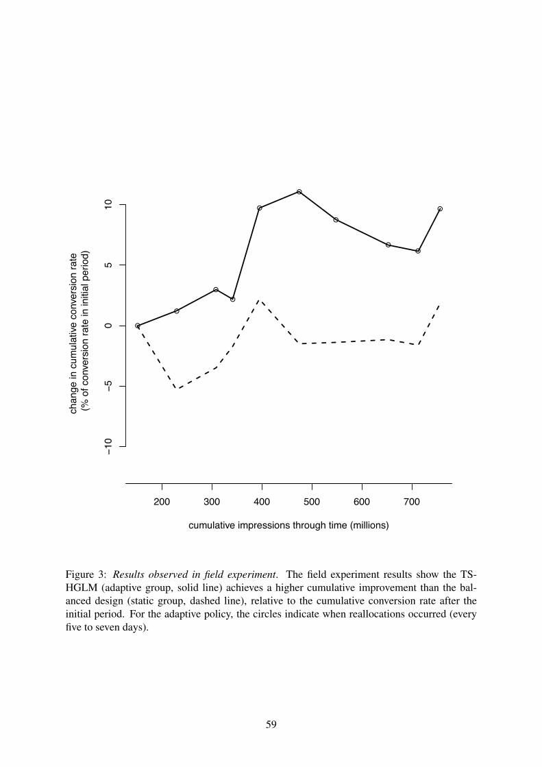
200 300 400 500 600 700
−10
−50
510
●
●
●
●
●
●
●
●●
●
cumulative impressions through time (millions)
chan
ge in
cum
ulat
ive c
onve
rsio
n ra
te
(% o
f con
vers
ion
rate
in in
itial
per
iod)
Figure 3: Results observed in field experiment. The field experiment results show the TS-HGLM (adaptive group, solid line) achieves a higher cumulative improvement than the bal-anced design (static group, dashed line), relative to the cumulative conversion rate after theinitial period. For the adaptive policy, the circles indicate when reallocations occurred (everyfive to seven days).
59

●●●●●●
●
●●●●● ●●●
●
Balanced
TS−BB−pooled
TS−GLM−pooled
TS−BB−unpooled
TS−LCGLM
TS−HGLM
Perfect Info
4.0 4.5 5.0 5.5 6.0
conversion rate (per million)
polic
y
Figure 4: Distributions of conversion rates following TS-based policies. The distributions of to-tal conversions for TS-based are compared. TS-HGLM performs better than the other versionsof TS with alternative model specifications, suggesting that the continuous parameter hetero-geneity across websites drives the improvement in performance. For all of the boxplots, thecenter line is the median, the box represents the interquartile range (IQR), the whiskers stretchto 1.5*IQR beyond the edges of the IQR, and the points are any values beyond the range of thewhiskers.
60

●●●●●●
●●●
●
●●●●● ●●●
Balanced
Gittins−pooled
Gittins−unpooled
UCB1−unpooled
UCBtuned−unpooled
TS−BB−unpooled
TS−HGLM
Perfect Info
4.0 4.5 5.0 5.5 6.0
conversion rate (per million)
polic
y
Figure 5: Distributions of conversion rates following Gittins index and Upper Confidence
Bound policies. The unpooled versions of TS, Gittins, and UCB-tuned policies outperformpooled policies as well as slightly outperforming the partially pooled TS-HGLM policy.
61

●●●●●●
●●
●● ●
●
Balanced
epsgreedy10−pooled
epsgreedy20−pooled
epsgreedy10−unpooled
epsgreedy20−unpooled
greedy−pooled
greedy−unpooled
TS−HGLM
Perfect Info
4.0 4.5 5.0 5.5 6.0
conversion rate (per million)
polic
y
Figure 6: Distributions of conversion rates following greedy and epsilon-greedy policies. Thedistributions of total conversions for greedy and epsilon-greedy policies are compared to theTS-HGLM policy and the balanced design policy. Setting epsilon to 20% performs better thansetting it to 10%.
62

●●●●●●
● ●
●●
●
●● ●
●●● ●
●
●
●
●●
●
●
Balanced
testrollout−t1
testrollout−t2
testrollout−t3
testrollout−t4
testrollout−t5
testrollout−t6
testrollout−unpooled−t1
testrollout−unpooled−t2
testrollout−unpooled−t3
testrollout−unpooled−t4
testrollout−unpooled−t5
testrollout−unpooled−t6
Perfect Info
4.0 4.5 5.0 5.5 6.0
conversion rate (per million)
polic
y
Figure 7: Distributions of conversion rates following test-rollout policies. The distributionsof total conversions for test-rollout policies are compared to the TS-HGLM policy and thebalanced design policy. Testing for only two initial periods yields better performance thantesting for any other length of time between 1 and 6 periods.
63

●●●●●●
●
●
●
●●●●● ●●●
Balanced
testrollout−unpooled−t2
epsgreedy10−unpooled
epsgreedy20−unpooled
greedy−unpooled
Gittins−unpooled
UCBtuned−unpooled
TS−BB−unpooled
Perfect Info
4.0 4.5 5.0 5.5 6.0
conversion rate (per million)
polic
y
Figure 8: Comparing unpooled policies. The relatively small differences among the unpooledpolicies suggest that allocation rule has less impact on performance than the level of model(pooled versus unpooled). Within unpooled policies, even simple heuristics, such as greedyand epsilon-greedy, perform well.
64

●
●●
●
●● ●●●
●●●
●● ● ● ●
●● ●
●
●●
●●
●
●
●●
●●●●
●●
●●
●
●●●
●
● ●●●
● ●●
●
●●
●
●●
●● ●●
●
●
●
●
● ●●●
● ●●
●
●●
●
●
●● ●
●
●
●
●● ●●
●
●● ●
●
●●
●●
●●
●
●
●●●
●●●
●
● ●●
● ●●
●●
●
●
●
●
●
●
●●
●● ●
●
●
●● ●
●
●
●
● ●
●●
●●●
●●●
●● ●
●
●● ●
●●
●●
●
●
●● ●
●●
●●
●● ●
●
●
●
●
●
●●
●
●
●● ●
●
●●
●●●●
●●●
● ●
●●
●●● ●●●
●
●●
● ●●
●
●●●
●
●●
●
●
●
●●
●
●●
●●
● ●
●
●●
●
●
●
● ●●
● ●●●
●●●●
●
●●
●
●●●●
●
●
●●
●
●● ●
● ●
●
● ●●●●●
●●●
●
●
●
●
●
●●
●
●
●●● ●●●●●●● ●
● ●●
●●●
●
●
●●●●●
●●
●
●● ●
● ●●●●● ●
●
●●
● ●●
●●
●
●●
●
●●
●
●●●
●
Obs. conversion rate (powers of 10)
Obs
. clic
k th
roug
h ra
te (p
ower
s of
10)
−7 −6 −5 −4
−5−4
−3
Figure 9: Click through rate versus conversion rate scatter plot. The best ads for conversionrate are not necessarily the best for click through rate. There is a weak correlation betweenclick through rate and conversion rate across the 532 unique website-size-concept combinations(correlation = -0.024, not significant, 95%CI = [-0.109, 0.061]). The points on the far leftrepresent the 200 observations with zero conversions throughout the experiment (and wouldnot have been shown on the log scale).
65

conversion rate (log−odds)
ad c
once
pt
size_160x600
●
●
●
●
30%
27%
19%
23%
●
●
●
●
24%
17%
26%
33%
●
●
●
●
27%
25%
22%
27%
●
●
●
●
30%
16%
28%
27%
−16 −14 −12 −10 −8
size_300x250
●
●
●
●
1%
22%
41%
37%
●
●
●
●
1%
30%
52%
18%
●
●
●
●
16%
33%
27%
23%
●
●
●
●
21%
22%
41%
15%
−16 −14 −12 −10 −8
size_728x90
●
●
●
●
10%
8%
26%
57%
●
●
●
●
2%
31%
39%
28%
●
●
●
●
23%
18%
22%
37%
●
●
●
●
25%
20%
22%
33%
−16 −14 −12 −10 −8
j103_t1j103_t6
j149_t1j149_t6
ad size A ad size B ad size C
Figure 10: Heterogeneity in conversion rates across websites and learning over time. Thelines represent the belief distributions of conversion rates, based on predictive distributions ofparameters from the HGLM (hierarchical logit model). Within each panel of a website j, timeperiod t, and an ad size, there are four ad concepts (horizontal lines, ordered from top to bottom,ad concepts 1 to 4). The allocation probabilities based on that model are printed (and shown bylevel of transparency of shading, from invisible 0% to opaque 100%). The four vertical panelsshow two different websites at two different time periods. Heterogeneity is shown throughdifferences across the two websites (j) for the same time period. Learning is shown throughthe two time periods (t) for the same website.
66