Embed Size (px)
Citation preview
1
Stats 2035 Midterm #2 Booklet Solutions G. Z-Based Confidence Intervals. Example 1.
(a) Set up a 99% confidence interval for the true population mean amount of paint contained in 5-litre cans.
1.0 , 50n , 975.4x .
01.0 , 576.22/ z .
The 99% confidence interval for is
0364.0975.450
1.0576.2975.4576.2
2/
nx
nzx
)011.5,939.4( .
(b) No, the manager cannot complain to the manufacturer because he can be 99% certain that the true mean lies between
L939.4 and L011.5 .
Example 2. (a) 100 , 64n , 350x .
05.0 , 2/z 96.1 .
The 95% confidence interval for is
)5.374,5.325(5.2435064
10096.135096.1
2/
nx
nzx
2
(b) No, since the 95% confidence interval does not contain the claimed mean of 400 hours. We are 97.5% certain that the true mean lifetime is less than 400 hours.
Example 3.
3 / 1.645 90% 3.2
0.2
/√
3.2 1.6450.2
√33.2 0.1899 3.01, 3.39
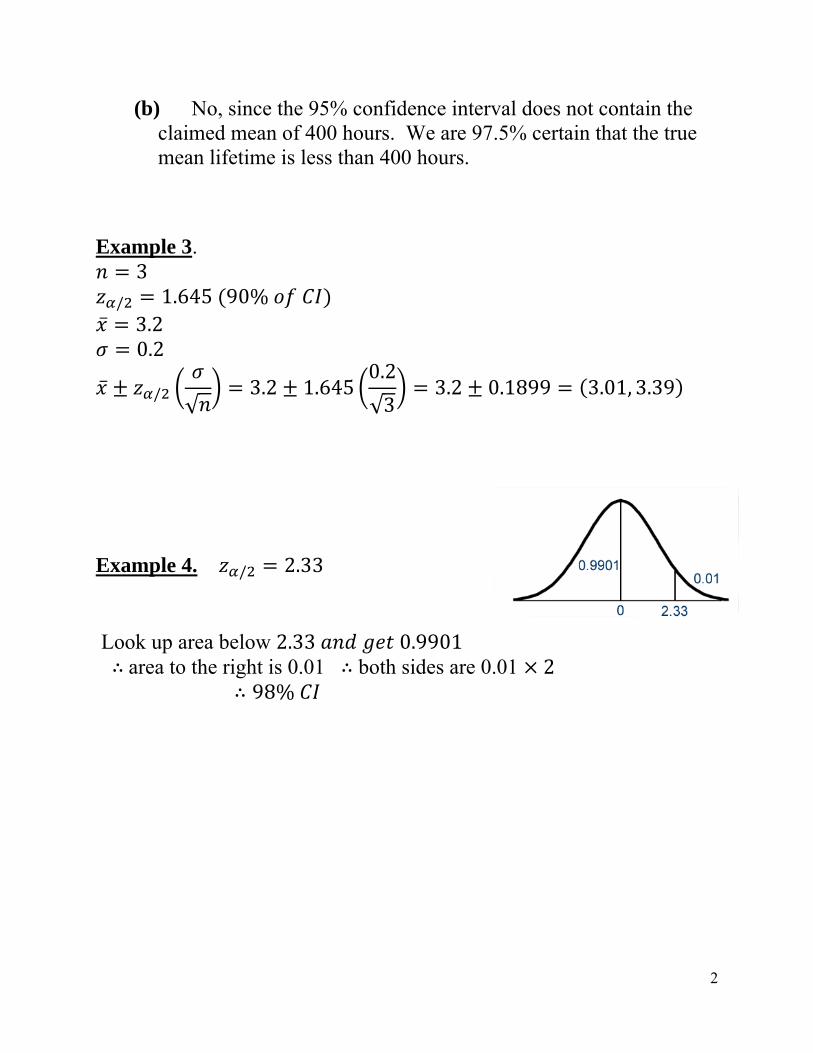
Example 4. / 2.33 Look up area below 2.33 0.9901 ∴area to the right is 0.01 ∴ both sides are 0.01 2 ∴ 98%
3
Example 5. 95% 86.52, 89.48
89.48 86.52
2.96 1.48
. . 88
∴ 1.48 1.96 2.576 1.945 ∴ 88 1.945, 88 1.945 86.06, 89.945
Example 6.
a) look up the area 0.97 (0.94 total on both sides around 0 and so there is 0.0.3 on each side) on the Z-table...you get Z=1.88
b) look up the area 0.98 on the Z-table...you get Z=2.05
G1. (a)
5.1904
762
4
0.1875.1950.1895.190
x .
14.3 , 4n .
10.0 , 645.12/z .
The 90% confidence interval for is
58.25.1904
14.3645.15.190645.1
2/
nx
nzx
)1.193,9.187( .
4
(b) The 90% confidence interval for would now be
17.55.1901
14.3645.15.190645.1
2/
nx
nzx
)7.195,3.185( .
(c) has been changed from 10.0 to 01.0 , so now 576.22/z .
The 99% confidence interval for is therefore
04.45.1904
14.3576.25.190576.2
2/
nx
nzx
)5.194,5.186( . G2. (a)
10
80
540
n
x
589.58) (490.42,
58.4954010
8096.1540
2/
n
zx
(b)
605.14) (474.86,
14.6554010
80575.2540
2/
n
zx
5
This interval is wider since in order to be more confident that the interval contains the true population mean, we need a larger range at values.
G3. n=100, 16, 3 0.05, ⁄ . 1.96
16.59) (15.41,
59.016010
396.1162/
n
zx
G4. 12n , 12.61x , 24.62 05.0 ,
The 95% confidence interval for is
93.1312.6112
62.2496.112.6196.1
2/
nx
nzx
G5.
17n , 13.28x , 05.12 .
05.0 ,
The 95% confidence interval for is
73.513.2871
05.1296.113.2896.1
2/
nx
nzx
6
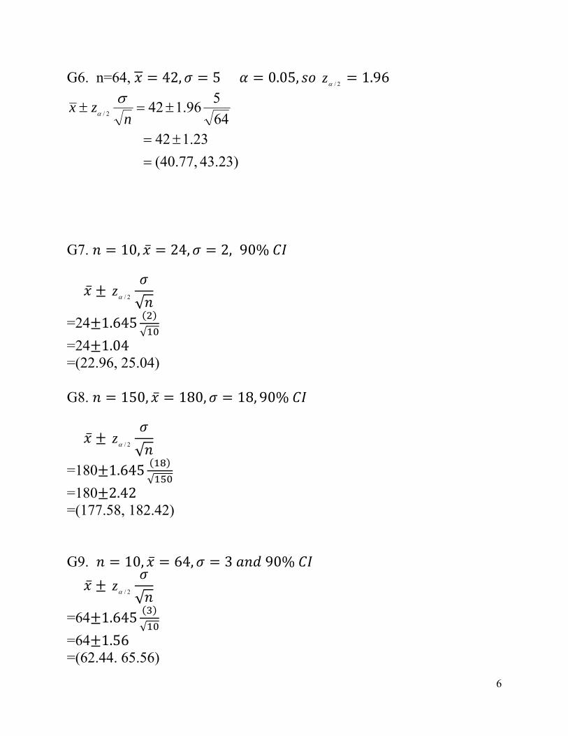
G6. n=64, 42, 5 0.05, 2/z 1.96
43.23) (40.77,
23.14264
596.142
2/
n
zx
G7. 10, 24, 2, 90%
2/z√
=24 1.645√
=24 1.04 =(22.96, 25.04) G8. 150, 180, 18, 90%
2/z√
=180 1.645√
=180 2.42 =(177.58, 182.42) G9. 10, 64, 3 90%
2/z√
=64 1.645√
=64 1.56 =(62.44. 65.56)
7
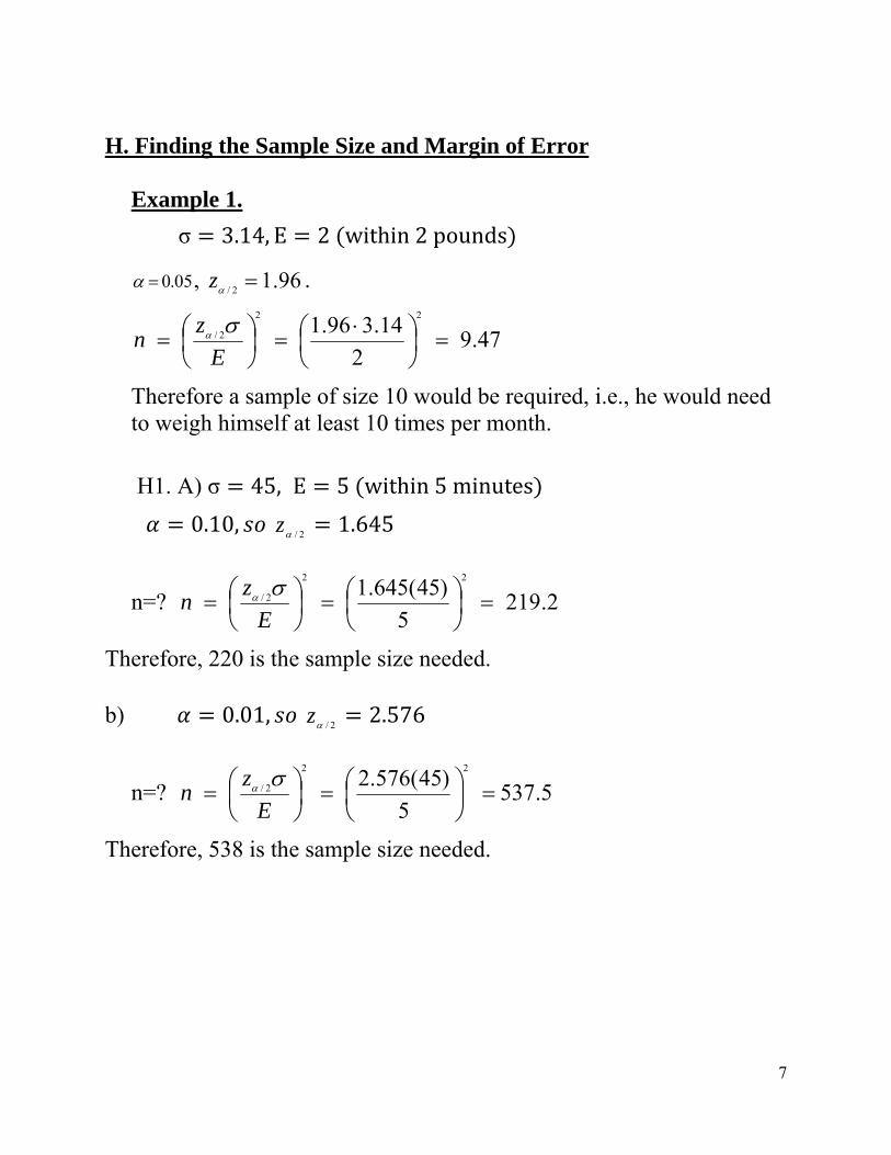
H. Finding the Sample Size and Margin of Error
Example 1.
σ 3.14, E 2 within2pounds
05.0 , 96.12/z .
47.92
14.396.122
2/
E
zn
Therefore a sample of size 10 would be required, i.e., he would need to weigh himself at least 10 times per month.
H1. A) σ 45, E 5 within5minutes
0.10, 2/z 1.645
n=? 2.2195
)45(645.122
2/
E
zn
Therefore, 220 is the sample size needed. b) 0.01,
2/z 2.576
n=? 5.5375
)45(576.222
2/
E
zn
Therefore, 538 is the sample size needed.
8
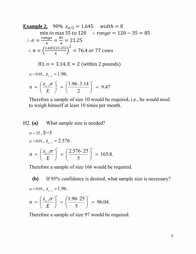
Example 2. 90% / 1.645 8 min max 35 120 ∴ 120 35 85
∴ 21.25
∴ . . 76.4 77
H1. σ 3.14, E 2 within2pounds
05.0 , 96.12/z .
47.92
14.396.122
2/
E
zn
Therefore a sample of size 10 would be required, i.e., he would need to weigh himself at least 10 times per month.
H2. (a) What sample size is needed?
25 , E=5
01.0 , 576.22/z .
8.1655
25576.222
2/
E
zn
.
Therefore a sample of size 166 would be required.
(b) If 95% confidence is desired, what sample size is necessary?
05.0 , 96.12/z .
04.965
2596.122
2/
E
zn
.
Therefore a sample of size 97 would be required.
9
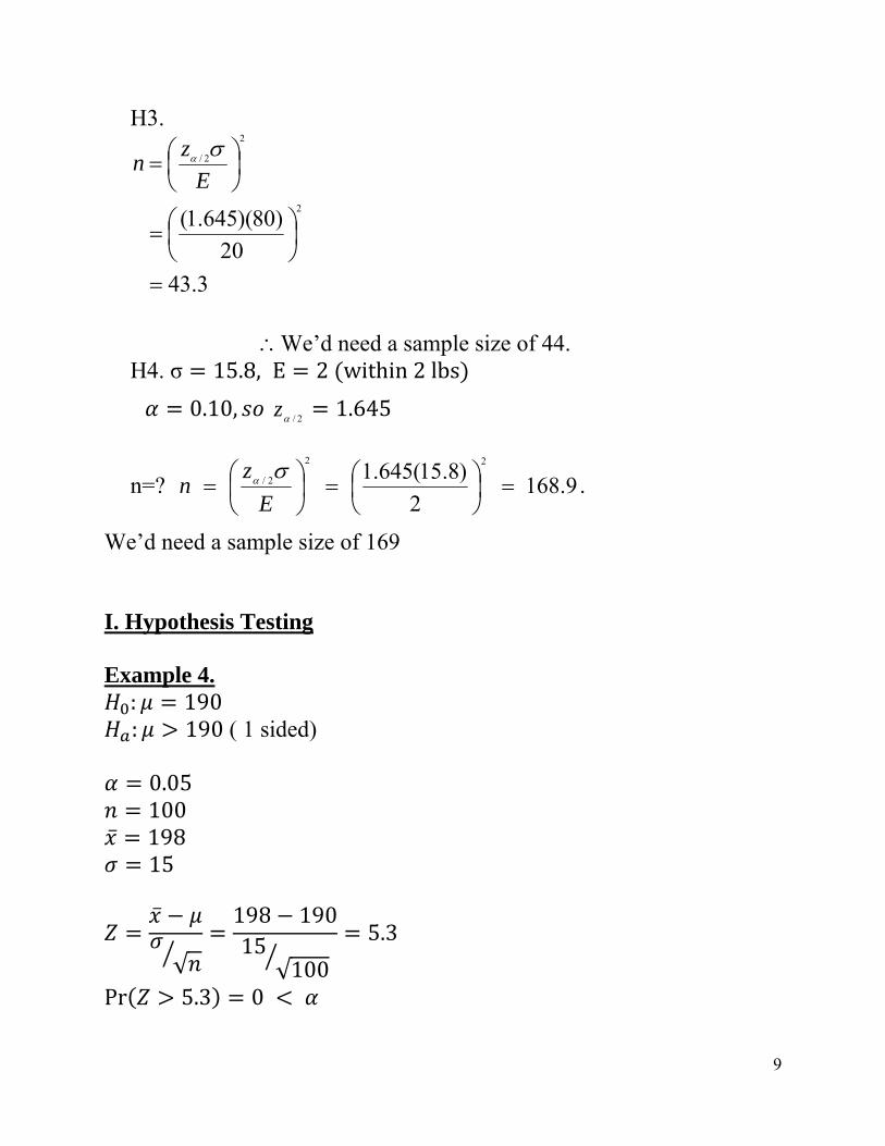
H3.
3.43
20
)80)(645.1(2
2
2/
E
zn
We’d need a sample size of 44.
H4. σ 15.8, E 2 within2lbs
0.10, 2/z 1.645
n=? 9.1682
)8.15(645.122
2/
E
zn
.
We’d need a sample size of 169 I. Hypothesis Testing Example 4. : 190 : 190 ( 1 sided)
0.05 100
198 15
√
198 19015
√100
5.3
Pr 5.3 0
10
∴ ˆ statistically significant evidence Example 5. : 7.7 : 7.7
50
7.5 0.5
√
7.5 7.70.5
√50
2.83
Pr 2.83 0.0023 1% chart p. 95 ∴ ∴ , there is stat. evidence that smokers need less sleep Example 6. : 50 : 50 ∴ 2 0.05 40
51 2
√
51 502√40
3.16
Pr 3.16 0.0008 2 0.0008 0.0016
11
∴
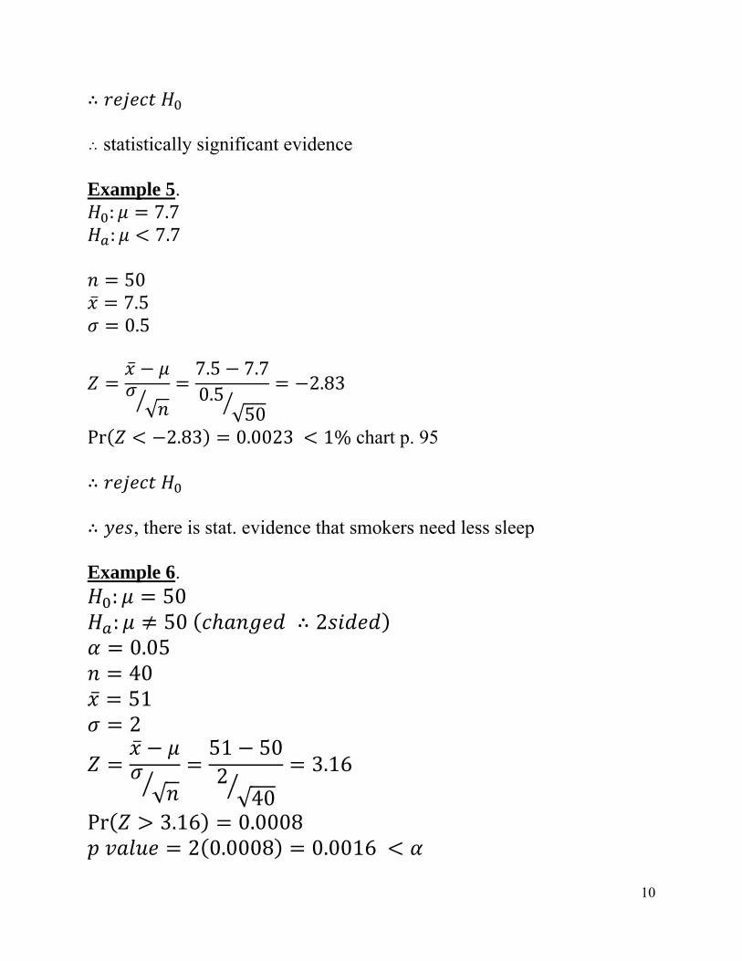
I1. (a) 250:H0 vs. 250:H a .
(b)
50n , 5.249x , 5.4 , 2500 .
05.0 , 645.12/z .
79.064.0
5.0
50/5.4
2505.249
/0
n
xz
.
Since this is a one-tailed test and 79.0z is not smaller than the critical value 645.1 z ( 2/zz ), therefore we fail to reject 0H . There is not enough evidence to suggest that the mean amount dispensed is less than 250 millilitres.
Alternatively, the p-value is 2148.0)79.0Pr( Zp .
Since the p-value 2148.0p is not less than 05.0 , we do not reject the null hypothesis.
I2. (a) True. The smaller the margin of error is, the less confidence we have in the ability of our interval to catch the population proportion.
(b) True. Larger samples are less variable, which translates to a smaller margin of error. We can be more precise at the same level of confidence.
12
(c) True. Smaller samples are more variable, leading us to be less confident in the ability of our interval to catch the true population proportion.
(d) True. The margin of error decreases as the square root of the sample size increases.
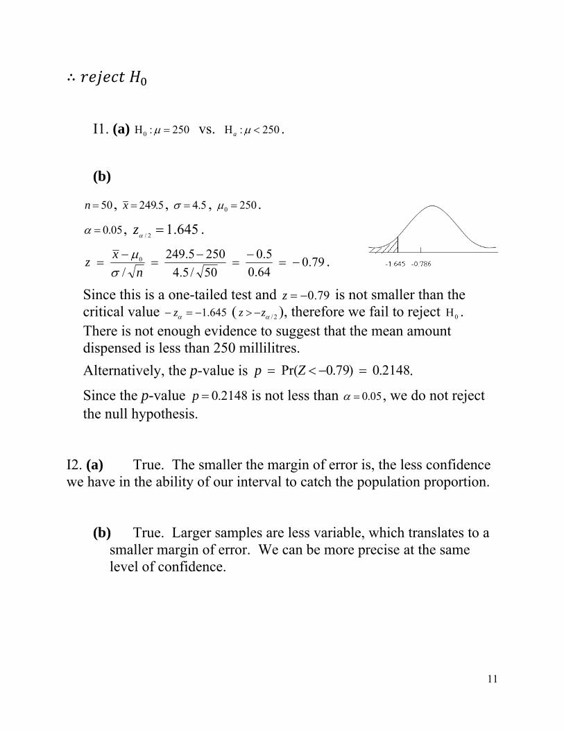
I3. H0 500 Ha 500 n=50, =96, 535
√⁄=
√⁄=2.57
Method 1: Draw the rejection
region and see if Z=2.57 lies in it
Reject H0 if Z>1.645 at
0.05 Since Z=2.57>1.645, we reject H0
Therefore, there is reason to believe the process increases the yield. Method 2: Calculate the p-value Area=p-value= Pr(Z>2.57) = 1 - 0.9949 = 0.0051 p-value<0.05 and we reject H0
13
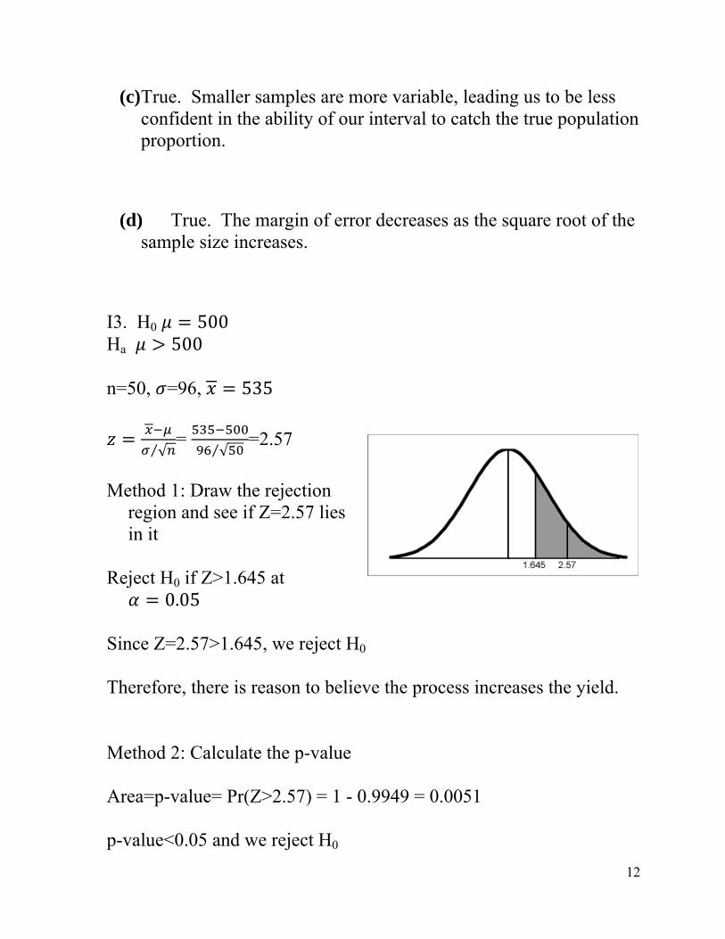
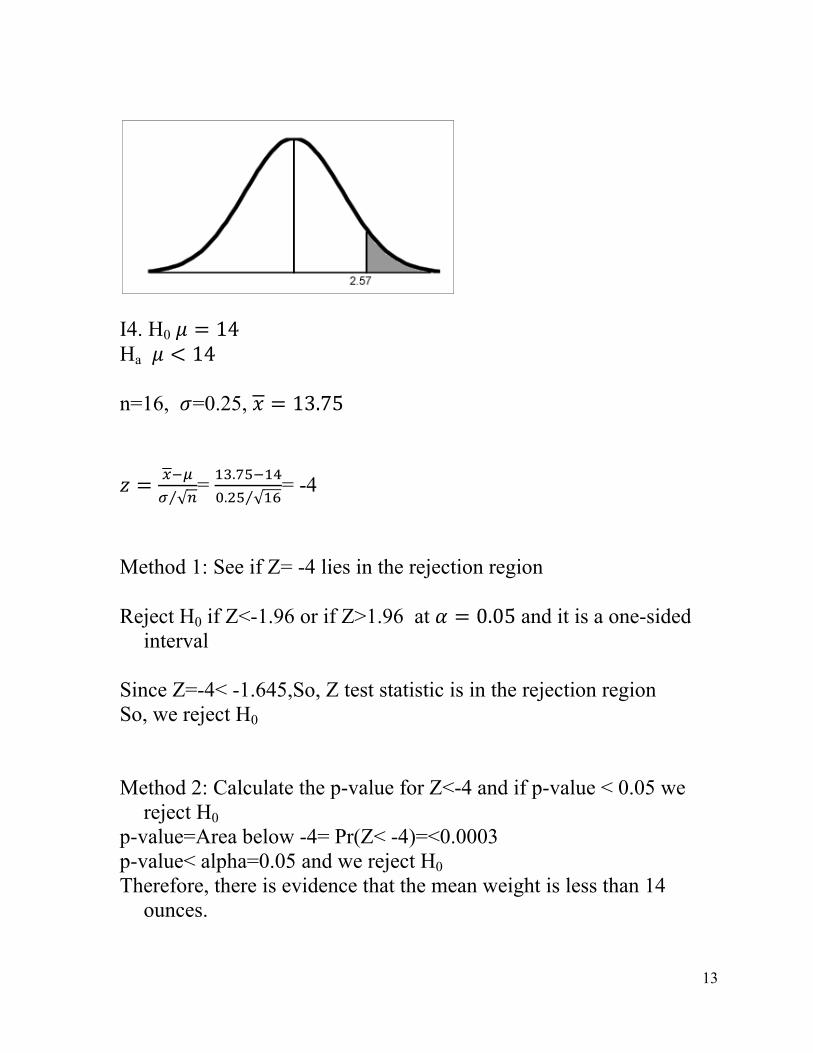
I4. H0 14 Ha 14 n=16, =0.25, 13.75
√⁄=
.
. √⁄= -4
Method 1: See if Z= -4 lies in the rejection region Reject H0 if Z<-1.96 or if Z>1.96 at 0.05 and it is a one-sided
interval Since Z=-4< -1.645,So, Z test statistic is in the rejection region So, we reject H0
Method 2: Calculate the p-value for Z<-4 and if p-value < 0.05 we
reject H0
p-value=Area below -4= Pr(Z< -4)=<0.0003 p-value< alpha=0.05 and we reject H0
Therefore, there is evidence that the mean weight is less than 14 ounces.
14
I5. a) The Confidence interval is not related to the sample mean and
different samples result in different intervals. b) This one is True. c) A confidence interval is about the mean salary of the population of
Nevada teachers, not the salaries of individual teachers. d) A confidence interval doesn't tell us about the sample or about
individual teachers. e) Nevada is the population we want to know about, not the entire
United States. I6.a) State the null and alternative hypotheses.
32:H
32:Ho
a
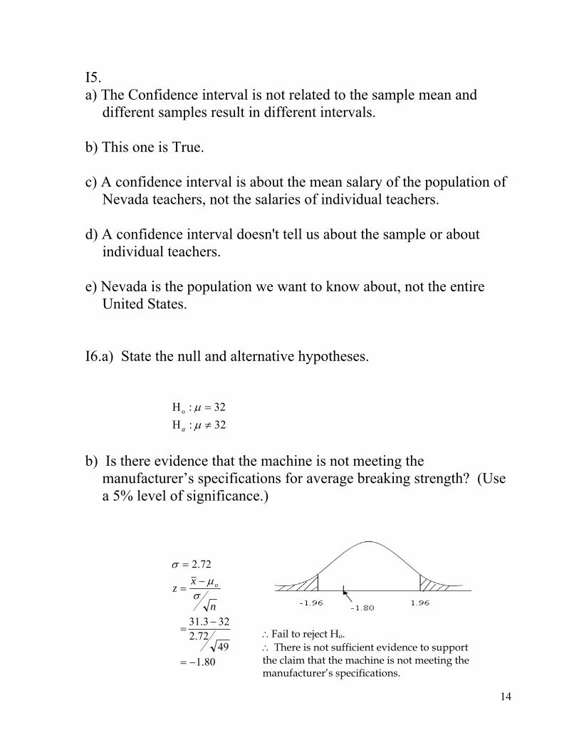
b) Is there evidence that the machine is not meeting the
manufacturer’s specifications for average breaking strength? (Use a 5% level of significance.)
80.149
72.2323.31
72.2
n
xz o
Fail to reject Ho. There is not sufficient evidence to support the claim that the machine is not meeting the manufacturer’s specifications.
15
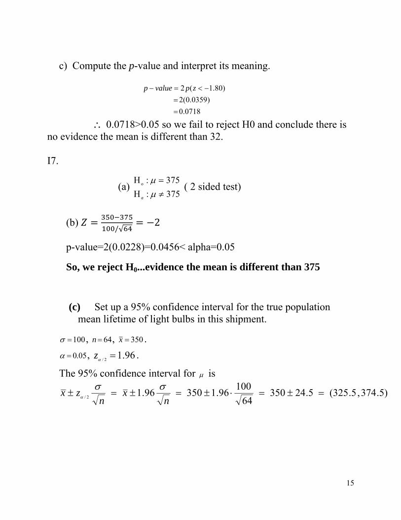
c) Compute the p-value and interpret its meaning.
0718.0
)0359.0(2
)80.1(2
zpvaluep
0.0718>0.05 so we fail to reject H0 and conclude there is no evidence the mean is different than 32. I7.
(a) 375:H
375:Ho
a
( 2 sided test)
(b) /√
2
p-value=2(0.0228)=0.0456< alpha=0.05
So, we reject H0...evidence the mean is different than 375
(c) Set up a 95% confidence interval for the true population mean lifetime of light bulbs in this shipment.
100 , 64n , 350x .
05.0 , 96.12/z .
The 95% confidence interval for is
)5.374,5.325(5.2435064
10096.135096.1
2/
nx
nzx
16
J. Confidence Intervals and Z-Tests for a Population Proportion
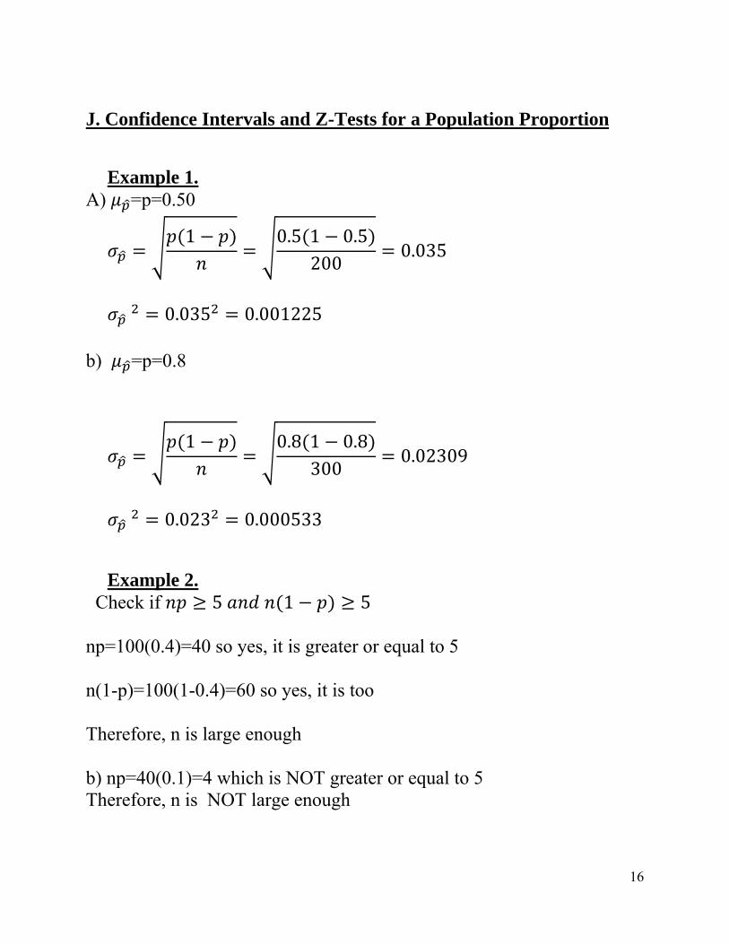
Example 1. A) =p=0.50
1 0.5 1 0.5200
0.035
0.035 0.001225
b) =p=0.8
1 0.8 1 0.8300
0.02309
0.023 0.000533
Example 2. Check if 5 1 5 np=100(0.4)=40 so yes, it is greater or equal to 5 n(1-p)=100(1-0.4)=60 so yes, it is too Therefore, n is large enough b) np=40(0.1)=4 which is NOT greater or equal to 5 Therefore, n is NOT large enough
17
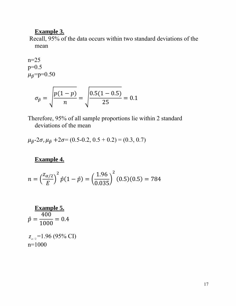
Example 3. Recall, 95% of the data occurs within two standard deviations of the
mean n=25 p=0.5
=p=0.50
1 0.5 1 0.525
0.1
Therefore, 95% of all sample proportions lie within 2 standard
deviations of the mean
-2 , 2 = (0.5-0.2, 0.5 + 0.2) = (0.3, 0.7)
Example 4.
/ 1
1.960.035
0.5 0.5 784
Example 5.
4001000
0.4
2/z =1.96 (95% CI) n=1000
18
2/z
1
=0.4 1.96 . .
=0.4 0.03 =(0.37, 0.43)
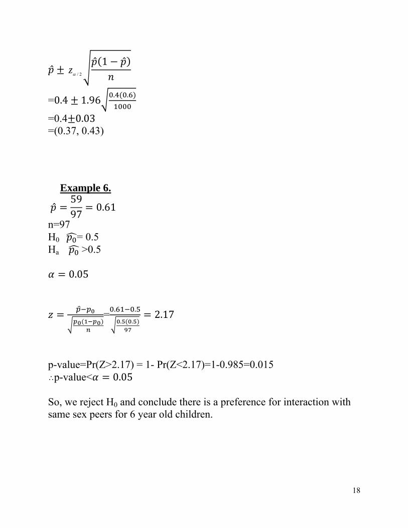
Example 6.
5997
0.61
n=97 H0 = 0.5 Ha >0.5
0.05
=. .
. .2.17
p-value=Pr(Z>2.17) = 1- Pr(Z<2.17)=1-0.985=0.015 ˆp-value< 0.05 So, we reject H0 and conclude there is a preference for interaction with same sex peers for 6 year old children.
19
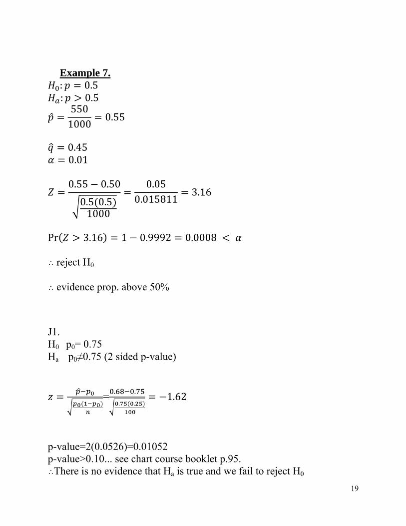
Example 7. : 0.5 : 0.5
5501000
0.55
0.45 0.01
0.55 0.50
0.5 0.51000
0.050.015811
3.16
Pr 3.16 1 0.9992 0.0008 ˆ reject H0 ˆ evidence prop. above 50%
J1. H0 p0= 0.75 Ha p0≠0.75 (2 sided p-value)
=. .
. .1.62
p-value=2(0.0526)=0.01052 p-value>0.10... see chart course booklet p.95. ˆThere is no evidence that Ha is true and we fail to reject H0
20
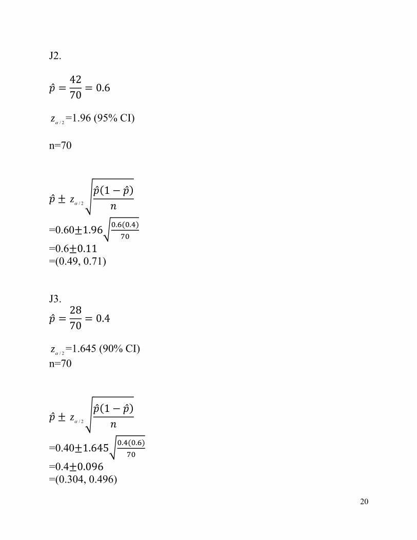
J2.
4270
0.6
2/z =1.96 (95% CI) n=70
2/z
1
=0.60 1.96 . .
=0.6 0.11 =(0.49, 0.71) J3.
2870
0.4
2/z =1.645 (90% CI) n=70
2/z
1
=0.40 1.645 . .
=0.4 0.096 =(0.304, 0.496)
21
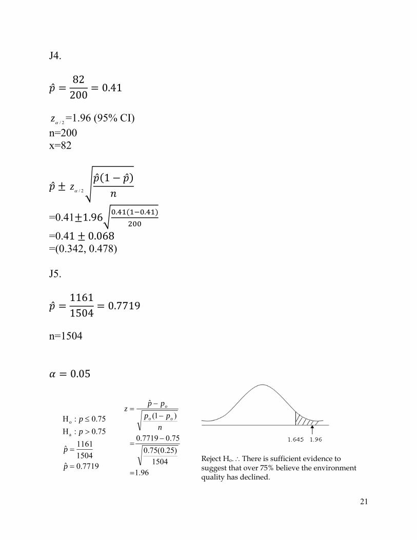
J4.
82200
0.41
2/z =1.96 (95% CI) n=200 x=82
2/z
1
=0.41 1.96 . .
=0.41 0.068 =(0.342, 0.478) J5.
11611504
0.7719
n=1504
0.05
7719.0ˆ1504
1161ˆ
75.0:H
75.0:H
a
o
p
p
p
p
96.11504
)25.0(75.0
75.07719.0
)1(
ˆ
n
pp
ppz
oo
o
Reject Ho. There is sufficient evidence to suggest that over 75% believe the environment quality has declined.
22
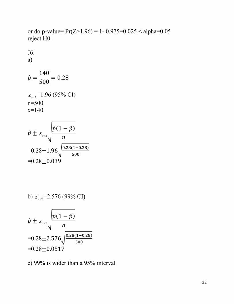
or do p-value= Pr(Z>1.96) = 1- 0.975=0.025 < alpha=0.05 reject H0. J6. a)
140500
0.28
2/z =1.96 (95% CI) n=500 x=140
2/z
1
=0.28 1.96 . .
=0.28 0.039 b)
2/z =2.576 (99% CI)
2/z
1
=0.28 2.576 . .
=0.28 0.0517 c) 99% is wider than a 95% interval
23
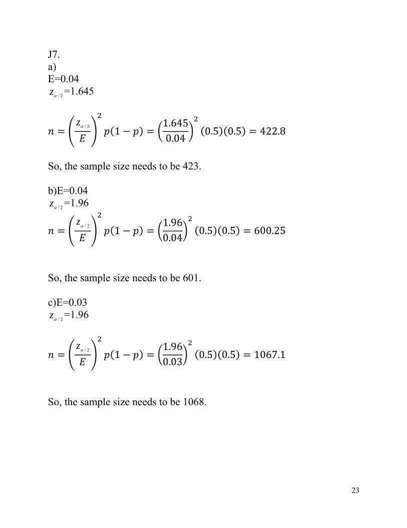
J7. a) E=0.04
2/z =1.645
2/z1
1.6450.04
0.5 0.5 422.8
So, the sample size needs to be 423. b)E=0.04
2/z =1.96
2/z1
1.960.04
0.5 0.5 600.25
So, the sample size needs to be 601. c)E=0.03
2/z =1.96
2/z1
1.960.03
0.5 0.5 1067.1
So, the sample size needs to be 1068.
24
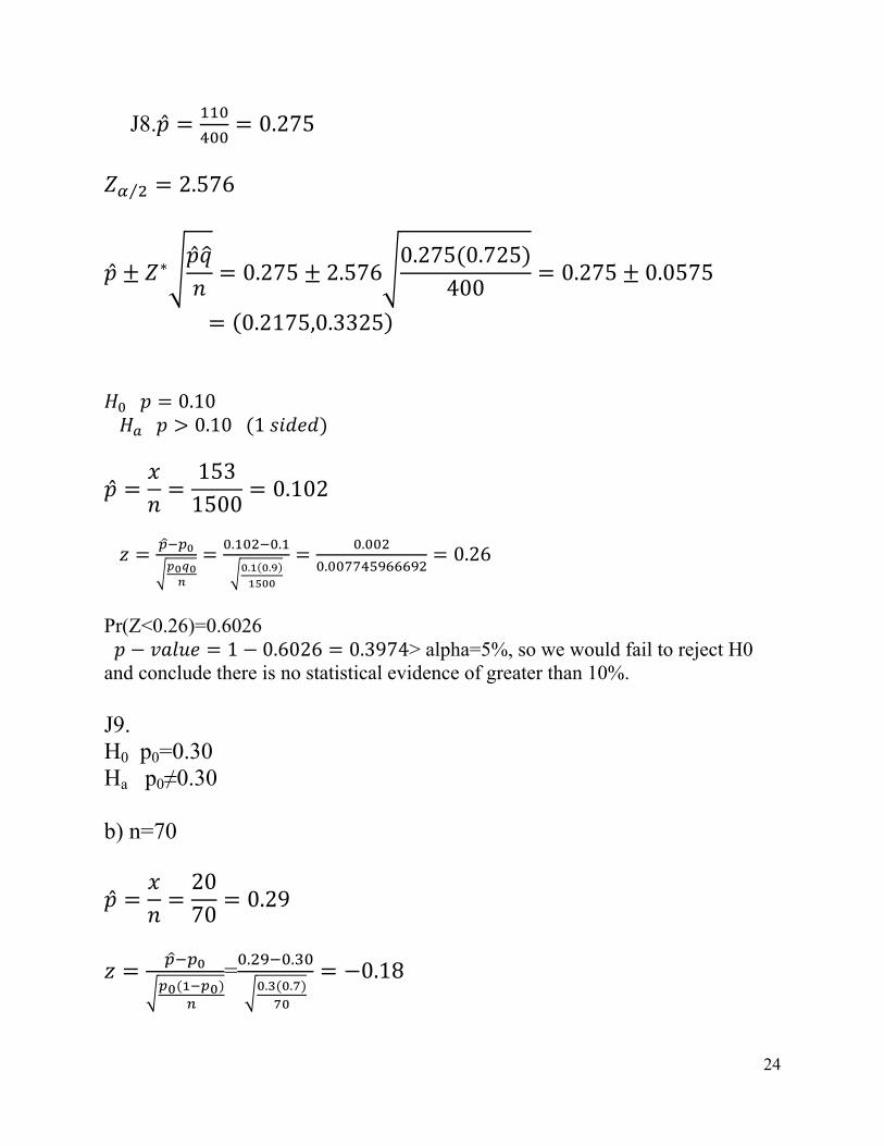
J8. 0.275
⁄ 2.576
∗ 0.275 2.576
0.275 0.725400
0.275 0.0575
0.2175,0.3325 0.10
0.10 1
1531500
0.102
. .
. .
.
.0.26
Pr(Z<0.26)=0.6026 1 0.6026 0.3974> alpha=5%, so we would fail to reject H0 and conclude there is no statistical evidence of greater than 10%. J9. H0 p0=0.30 Ha p0≠0.30 b) n=70
2070
0.29
=. .
. .0.18
25
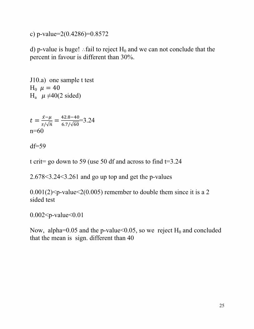
c) p-value=2(0.4286)=0.8572 d) p-value is huge! ˆfail to reject H0 and we can not conclude that the percent in favour is different than 30%. J10.a) one sample t test H0 40 Ha ≠40(2 sided)
/√
.
. /√=3.24
n=60 df=59 t crit= go down to 59 (use 50 df and across to find t=3.24 2.678<3.24<3.261 and go up top and get the p-values 0.001(2)<p-value<2(0.005) remember to double them since it is a 2 sided test 0.002<p-value<0.01 Now, alpha=0.05 and the p-value<0.05, so we reject H0 and concluded that the mean is sign. different than 40
26
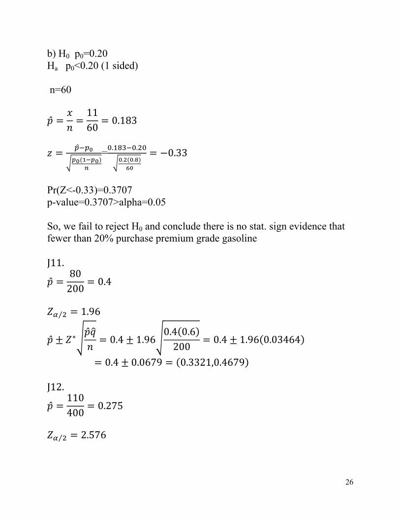
b) H0 p0=0.20 Ha p0<0.20 (1 sided) n=60
1160
0.183
=. .
. .0.33
Pr(Z<-0.33)=0.3707 p-value=0.3707>alpha=0.05 So, we fail to reject H0 and conclude there is no stat. sign evidence that fewer than 20% purchase premium grade gasoline J11.
80200
0.4
⁄ 1.96
∗ 0.4 1.96
0.4 0.6200
0.4 1.96 0.03464
0.4 0.0679 0.3321,0.4679 J12.
110400
0.275
⁄ 2.576
27
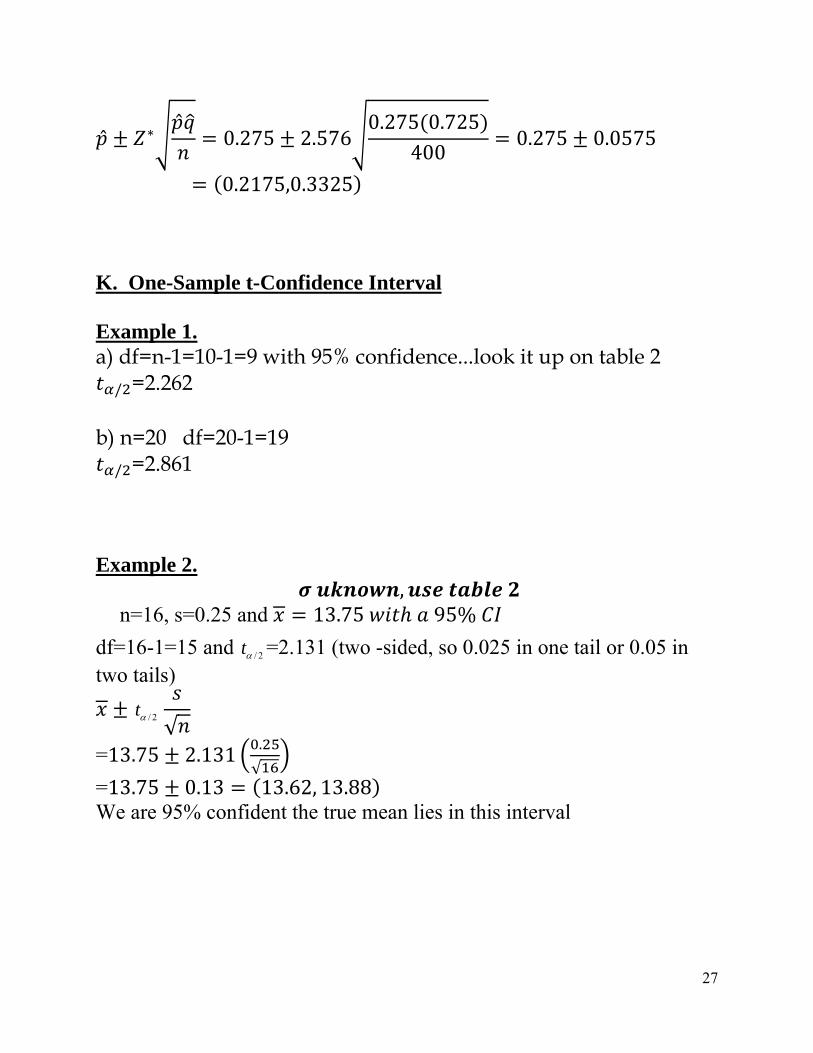
∗ 0.275 2.576
0.275 0.725400
0.275 0.0575
0.2175,0.3325 K. One-Sample t-Confidence Interval Example 1. a) df=n-1=10-1=9 with 95% confidence...look it up on table 2 / =2.262
b) n=20 df=20-1=19 / =2.861
Example 2.
, n=16, s=0.25 and 13.75 95%
df=16-1=15 and 2/t =2.131 (two -sided, so 0.025 in one tail or 0.05 in two tails)
2/t√
=13.75 2.131 .
√
=13.75 0.13 13.62, 13.88 We are 95% confident the true mean lies in this interval
28
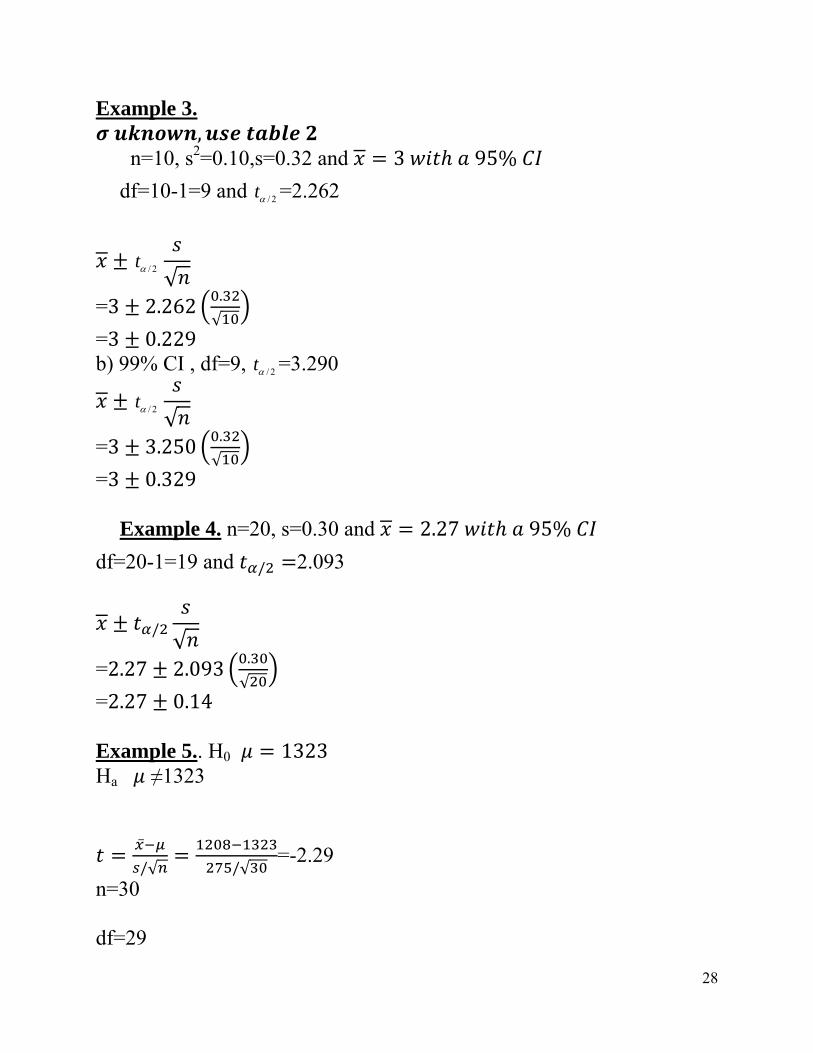
Example 3. , n=10, s2=0.10,s=0.32 and 3 95%
df=10-1=9 and 2/t =2.262
2/t√
=3 2.262 .
√
=3 0.229 b) 99% CI , df=9, 2/t =3.290
2/t√
=3 3.250 .
√
=3 0.329
Example 4. n=20, s=0.30 and 2.27 95%
df=20-1=19 and / 2.093
/√
=2.27 2.093 .
√
=2.27 0.14 Example 5.. H0 1323 Ha ≠1323
/√ /√=-2.29
n=30 df=29
29
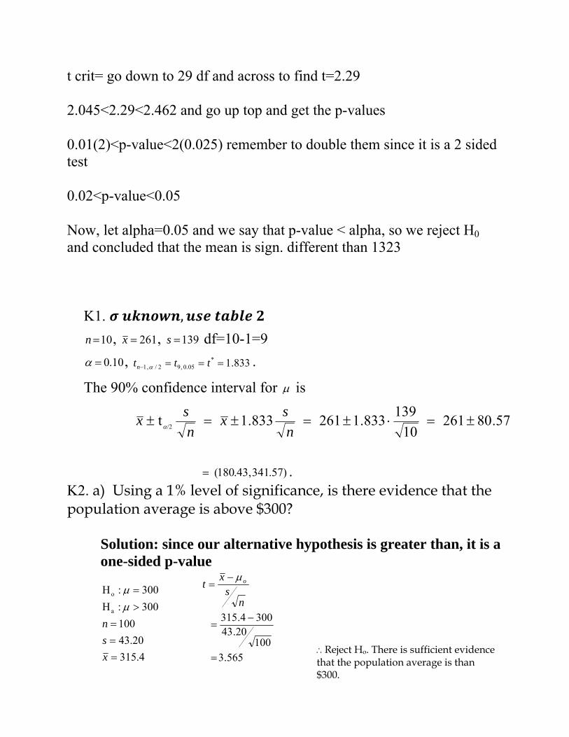
t crit= go down to 29 df and across to find t=2.29 2.045<2.29<2.462 and go up top and get the p-values 0.01(2)<p-value<2(0.025) remember to double them since it is a 2 sided test 0.02<p-value<0.05 Now, let alpha=0.05 and we say that p-value < alpha, so we reject H0 and concluded that the mean is sign. different than 1323
K1. ,
10n , 261x , 139s df=10-1=9
10.0 , 833.1*05.0,92/,1 tttn .
The 90% confidence interval for is
57.8026110
139833.1261833.1t
/2
n
sx
n
sx
)57.341,43.180( . K2. a) Using a 1% level of significance, is there evidence that the population average is above $300?
Solution: since our alternative hypothesis is greater than, it is a
one-sided p-value
4.315
20.43
100
300:H
300:H
a
o
x
s
n
565.3100
20.433004.315
ns
xt o
Reject Ho. There is sufficient evidence that the population average is than $300.
30
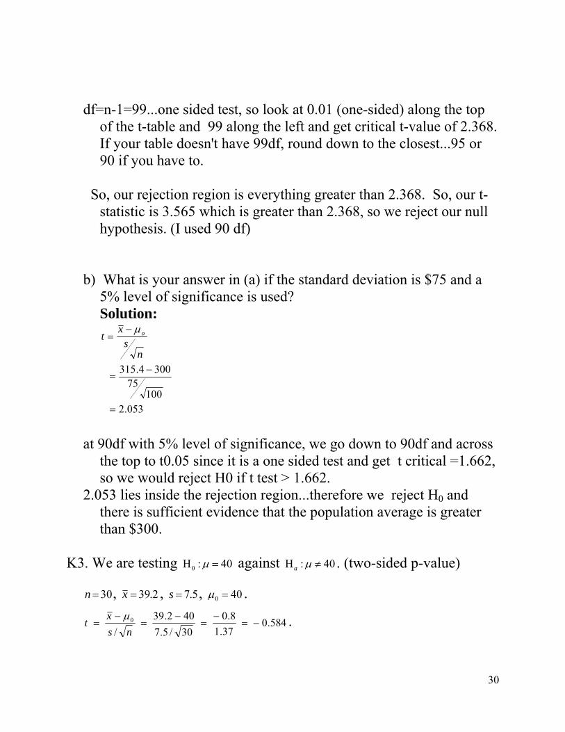
df=n-1=99...one sided test, so look at 0.01 (one-sided) along the top
of the t-table and 99 along the left and get critical t-value of 2.368. If your table doesn't have 99df, round down to the closest...95 or 90 if you have to.
So, our rejection region is everything greater than 2.368. So, our t-
statistic is 3.565 which is greater than 2.368, so we reject our null hypothesis. (I used 90 df)
b) What is your answer in (a) if the standard deviation is $75 and a
5% level of significance is used? Solution:
053.2100
753004.315
ns
xt o
at 90df with 5% level of significance, we go down to 90df and across
the top to t0.05 since it is a one sided test and get t critical =1.662, so we would reject H0 if t test > 1.662.
2.053 lies inside the rejection region...therefore we reject H0 and there is sufficient evidence that the population average is greater than $300.
K3. We are testing 40:H0 against 40:H a . (two-sided p-value)
30n , 2.39x , 5.7s , 400 .
584.037.1
8.0
30/5.7
402.39
/0
ns
xt
.
31
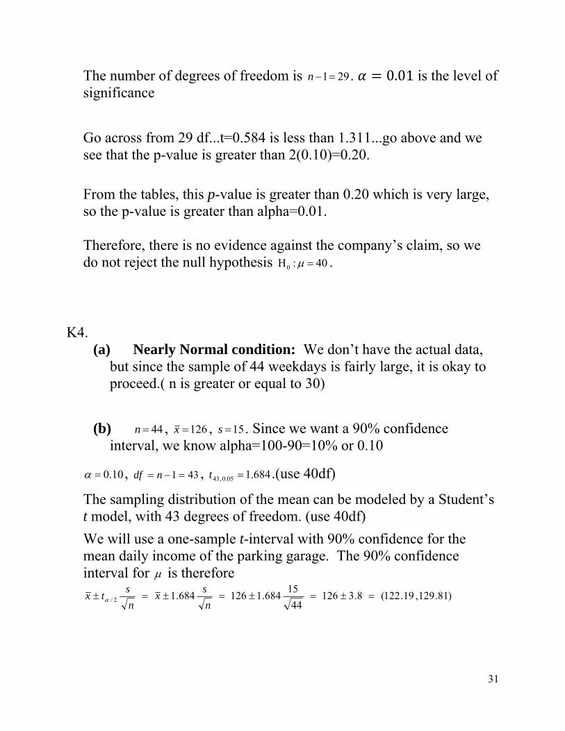
The number of degrees of freedom is 291n . 0.01 is the level of significance
Go across from 29 df...t=0.584 is less than 1.311...go above and we see that the p-value is greater than 2(0.10)=0.20.
From the tables, this p-value is greater than 0.20 which is very large, so the p-value is greater than alpha=0.01. Therefore, there is no evidence against the company’s claim, so we do not reject the null hypothesis 40:H0 .
K4. (a) Nearly Normal condition: We don’t have the actual data,
but since the sample of 44 weekdays is fairly large, it is okay to proceed.( n is greater or equal to 30)
(b) 44n , 126x , 15s . Since we want a 90% confidence
interval, we know alpha=100-90=10% or 0.10
10.0 , 431 ndf , 684.105.0,43 t .(use 40df)
The sampling distribution of the mean can be modeled by a Student’s t model, with 43 degrees of freedom. (use 40df)
We will use a one-sample t-interval with 90% confidence for the mean daily income of the parking garage. The 90% confidence interval for is therefore
)81.129,19.122(8.312644
15684.1126684.12/
n
sx
n
stx
32
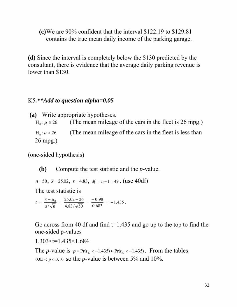
(c) We are 90% confident that the interval $122.19 to $129.81 contains the true mean daily income of the parking garage.
(d) Since the interval is completely below the $130 predicted by the consultant, there is evidence that the average daily parking revenue is lower than $130. K5.**Add to question alpha=0.05 (a) Write appropriate hypotheses.
26:H0 (The mean mileage of the cars in the fleet is 26 mpg.)
26:H a (The mean mileage of the cars in the fleet is less than 26 mpg.)
(one-sided hypothesis)
(b) Compute the test statistic and the p-value.
50n , 02.25x , 83.4s , 491 ndf . (use 40df)
The test statistic is
435.1683.0
98.0
50/83.4
2602.25
/0
ns
xt
.
Go across from 40 df and find t=1.435 and go up to the top to find the one-sided p-values
1.303<t=1.435<1.684
The p-value is )435.1Pr()435.1Pr( 5049 ttp . From the tables 10.005.0 p so the p-value is between 5% and 10%.
33
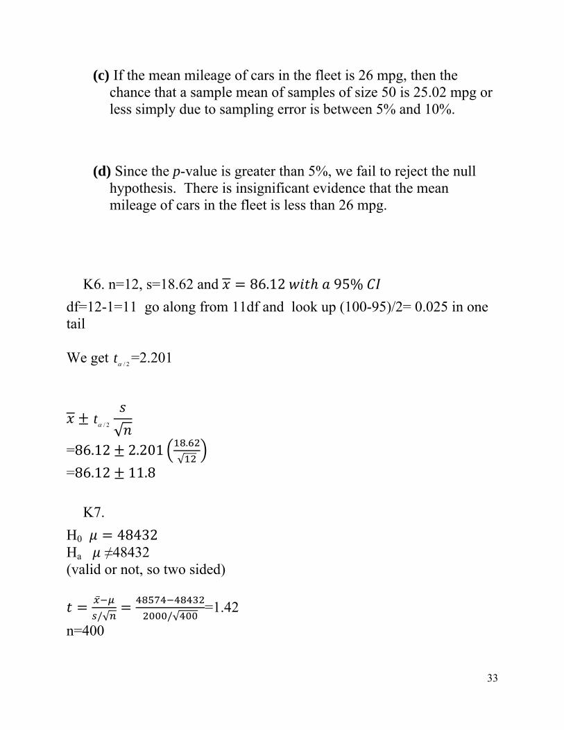
(c) If the mean mileage of cars in the fleet is 26 mpg, then the chance that a sample mean of samples of size 50 is 25.02 mpg or less simply due to sampling error is between 5% and 10%.
(d) Since the p-value is greater than 5%, we fail to reject the null hypothesis. There is insignificant evidence that the mean mileage of cars in the fleet is less than 26 mpg.
K6. n=12, s=18.62 and 86.12 95%
df=12-1=11 go along from 11df and look up (100-95)/2= 0.025 in one tail We get
2/t =2.201
2/t√
=86.12 2.201 .
√
=86.12 11.8
K7.
H0 48432 Ha ≠48432 (valid or not, so two sided)
/√ /√=1.42
n=400
34
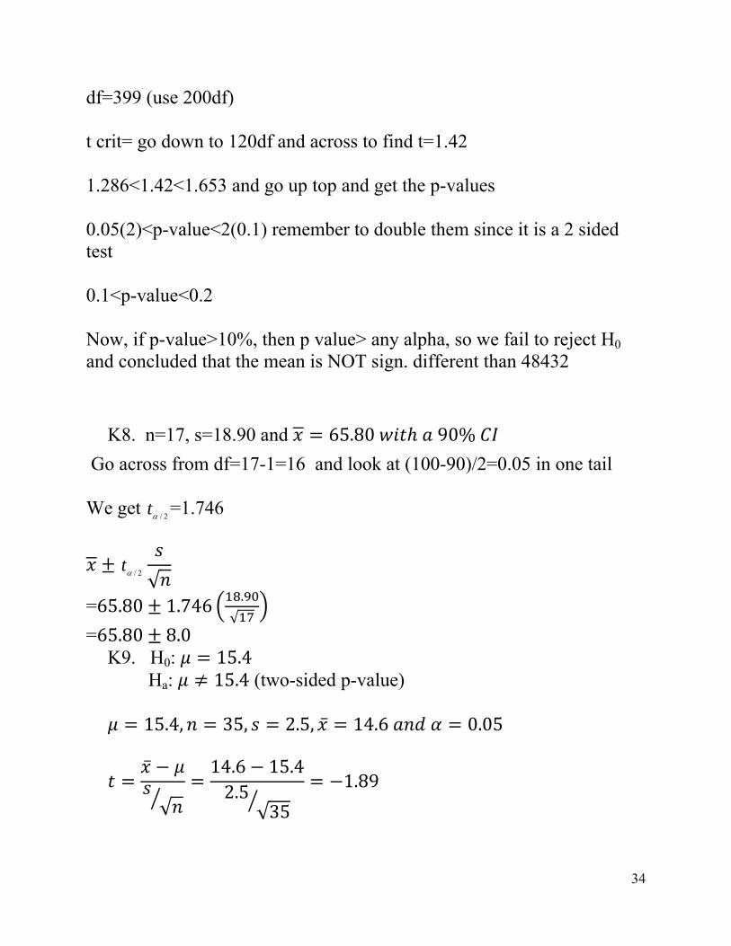
df=399 (use 200df) t crit= go down to 120df and across to find t=1.42 1.286<1.42<1.653 and go up top and get the p-values 0.05(2)<p-value<2(0.1) remember to double them since it is a 2 sided test 0.1<p-value<0.2 Now, if p-value>10%, then p value> any alpha, so we fail to reject H0 and concluded that the mean is NOT sign. different than 48432
K8. n=17, s=18.90 and 65.80 90%
Go across from df=17-1=16 and look at (100-90)/2=0.05 in one tail We get
2/t =1.746
2/t√
=65.80 1.746 .
√
=65.80 8.0 K9. H0: 15.4 Ha: 15.4 (two-sided p-value)
15.4, 35, 2.5, 14.6 0.05
√
14.6 15.42.5
√35
1.89
35
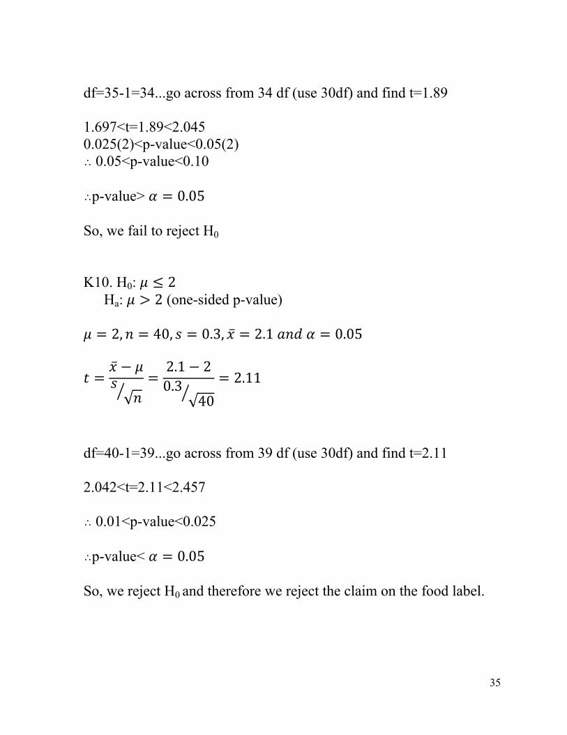
df=35-1=34...go across from 34 df (use 30df) and find t=1.89 1.697<t=1.89<2.045 0.025(2)<p-value<0.05(2) ˆ 0.05<p-value<0.10 ˆp-value> 0.05 So, we fail to reject H0 K10. H0: 2 Ha: 2 (one-sided p-value)
2, 40, 0.3, 2.1 0.05
√
2.1 20.3
√40
2.11
df=40-1=39...go across from 39 df (use 30df) and find t=2.11 2.042<t=2.11<2.457 ˆ 0.01<p-value<0.025 ˆp-value< 0.05 So, we reject H0 and therefore we reject the claim on the food label.
36
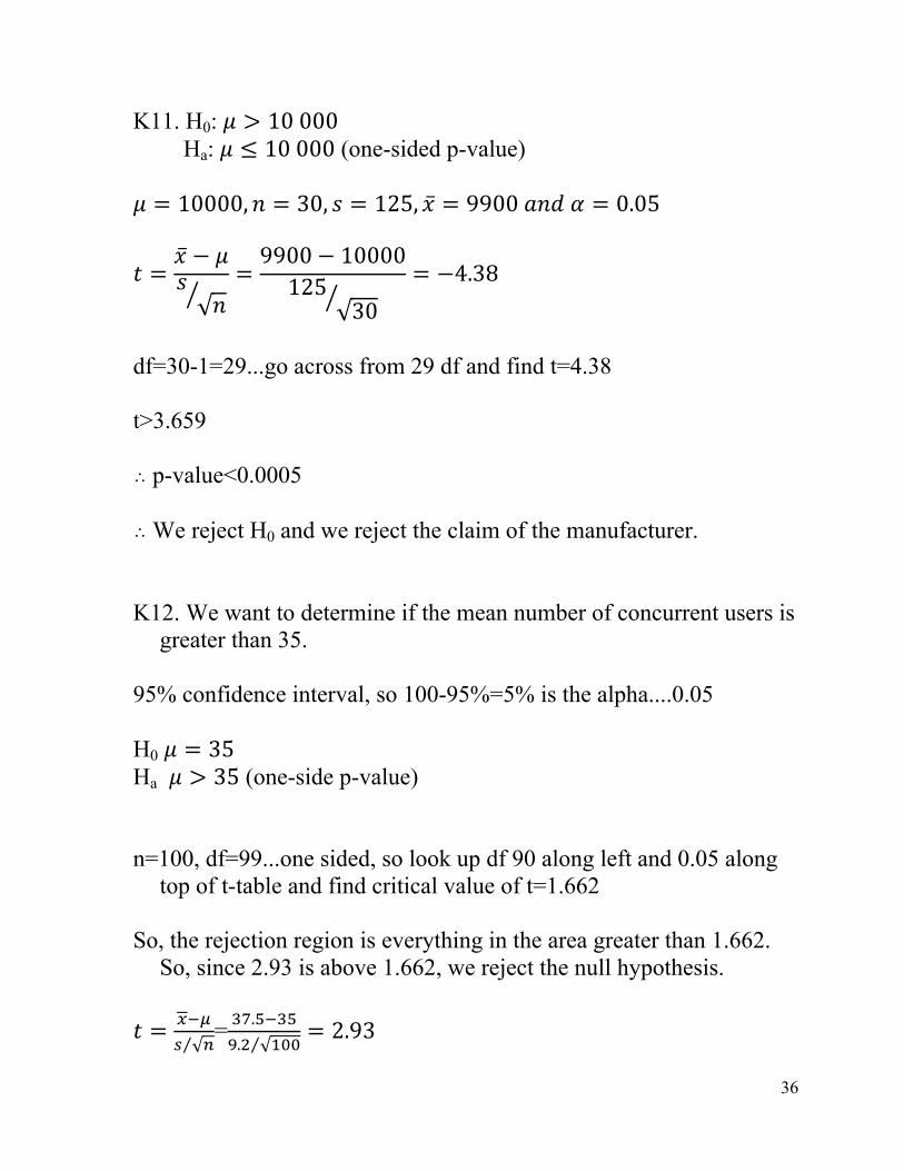
K11. H0: 10000 Ha: 10000 (one-sided p-value)
10000, 30, 125, 9900 0.05
√
9900 10000125
√30
4.38
df=30-1=29...go across from 29 df and find t=4.38 t>3.659 ˆ p-value<0.0005 ˆ We reject H0 and we reject the claim of the manufacturer. K12. We want to determine if the mean number of concurrent users is
greater than 35. 95% confidence interval, so 100-95%=5% is the alpha....0.05 H0 35 Ha 35 (one-side p-value) n=100, df=99...one sided, so look up df 90 along left and 0.05 along
top of t-table and find critical value of t=1.662 So, the rejection region is everything in the area greater than 1.662.
So, since 2.93 is above 1.662, we reject the null hypothesis.
√⁄=
.
. √⁄2.93
37
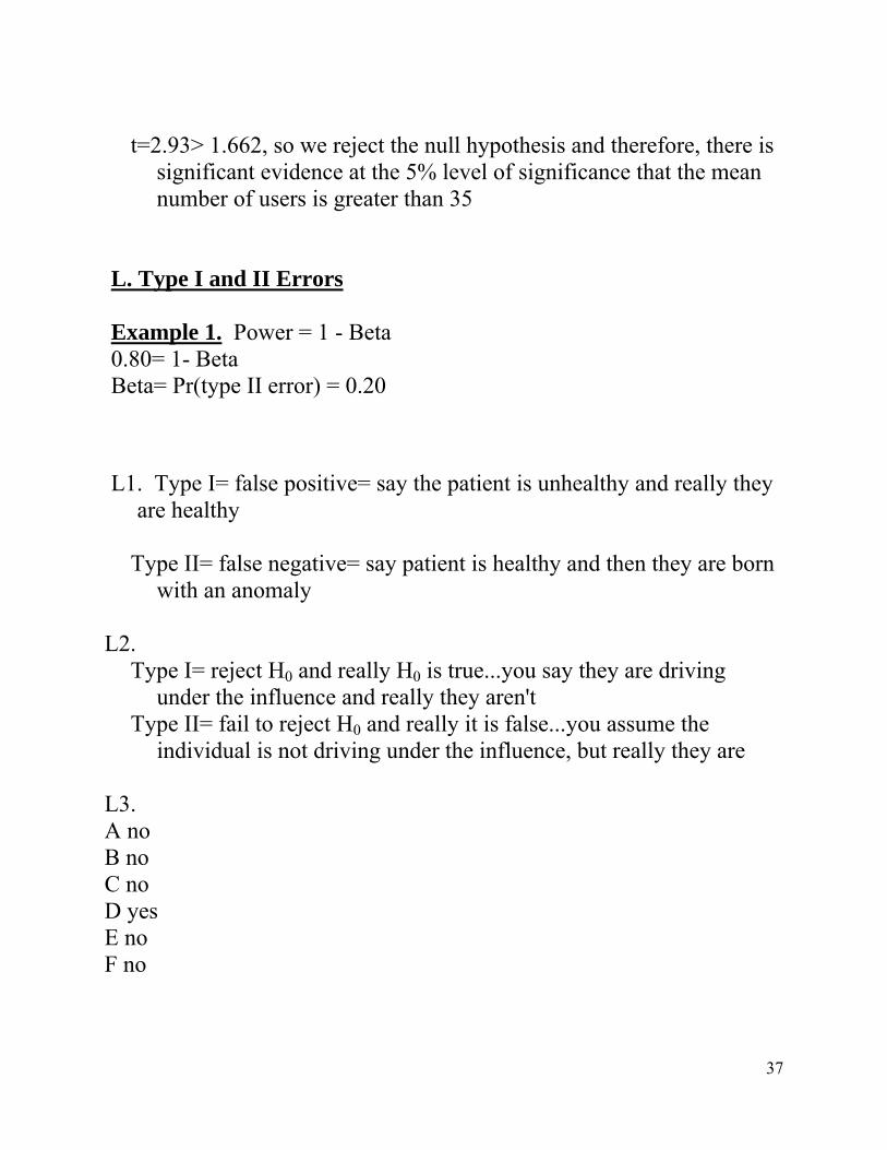
t=2.93> 1.662, so we reject the null hypothesis and therefore, there is
significant evidence at the 5% level of significance that the mean number of users is greater than 35
L. Type I and II Errors Example 1. Power = 1 - Beta 0.80= 1- Beta Beta= Pr(type II error) = 0.20
L1. Type I= false positive= say the patient is unhealthy and really they
are healthy Type II= false negative= say patient is healthy and then they are born
with an anomaly
L2. Type I= reject H0 and really H0 is true...you say they are driving
under the influence and really they aren't Type II= fail to reject H0 and really it is false...you assume the
individual is not driving under the influence, but really they are
L3. A no B no C no D yes E no F no
38
L4.
A type 1 error is to reject H0 when it is really true. So, in this case we would say the person has osteoporosis, but really they don't. The answer is B.
A type 2 error is when you fail to reject the null hypothesis and it should have been rejected because it is false. So, in this case we would say the person doesn't have osteoporosis, but they do in fact have it. So, the answer is A.
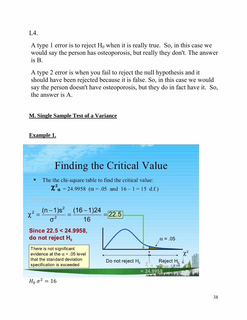
M. Single Sample Test of a Variance Example 1.
16
39
16 1- sided D.R reject H0 if 24.996 Therefore, do not reject H0 and there is no evidence that the standard deviation is exceeded Example 2. n=30 s=12.2 df=29 90% CI 1- 0.90 = 0.10
20.102
0.05
12
1,2
12
1,1 2
29 12.2229,0.05
29 12.2229,0.95
29 12.242.557
29 12.217.708
101.425 243.75
10.1 15.6 Example 3. 75
40
75 2 sided
alpha=0.05 n=35
crit = , , . 46.9792 (use 30)...upper bound
crit = , = , . 16.7908 ( use 30)...lower bound
DR. Reject H0 if 46.9792 16.7908
= 54.85
test So, 46.9792 ,
So, there is stat. evidence the variability is different than the general population M1. 20
20 (one- sided so do NOT divide alpha by 2)
n=20 s2=35 alpha=0.05 level of significance Since the test is one-sided,we only need the upper critical Chi square
crit = , = , . 30.1435
DR. reject H0 if 30.1435
41
= 33.25
test So, st >30.1435 so we reject H0 and conclude there is sign. evidence the variance is greater than 20 b) 45
45 (one- sided so do NOT divide alpha by 2)
n=8 s2=42 alpha=0.05 level of significance
crit = , = , . 2.16735...lower bound
DR.reject H0 if 2.16735
= 6.53
test So, st >2.16735 so we fail to reject H0 and conclude there is NO sign. evidence the variance is less than 45 c) 9
42
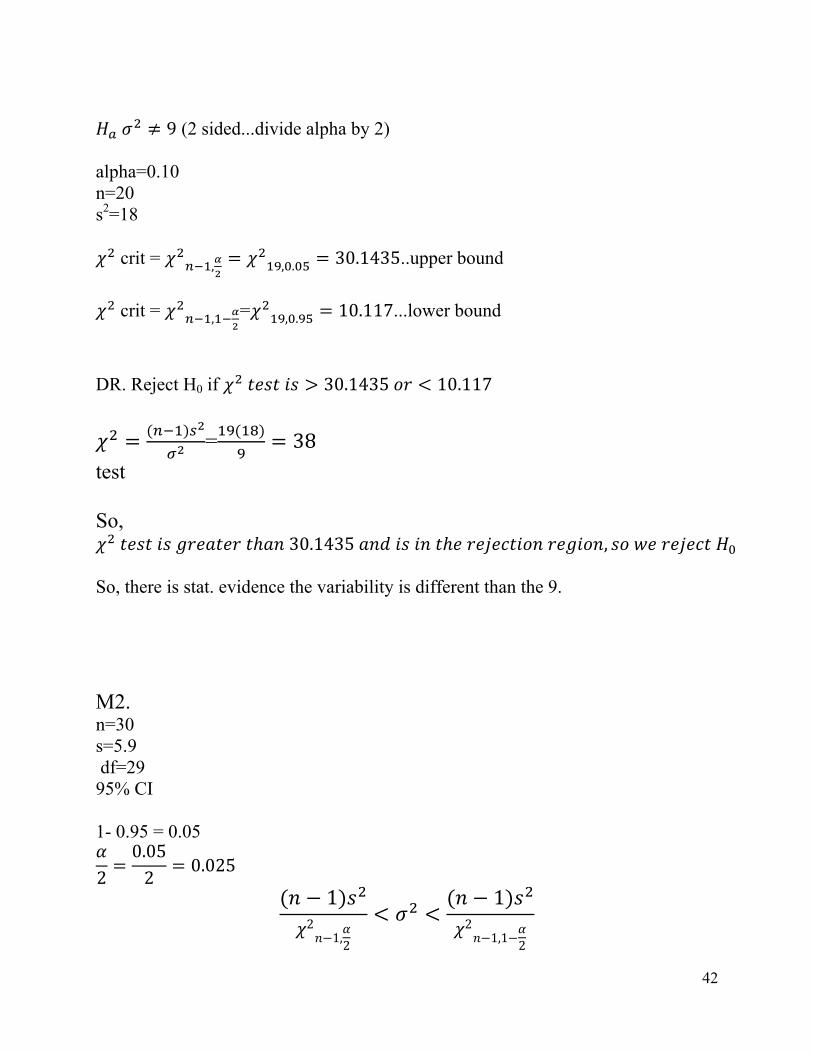
9 (2 sided...divide alpha by 2)
alpha=0.10 n=20 s2=18
crit = , , . 30.1435..upper bound
crit = , = , . 10.117...lower bound
DR. Reject H0 if 30.1435 10.117
= 38
test So, 30.1435 ,
So, there is stat. evidence the variability is different than the 9. M2. n=30 s=5.9 df=29 95% CI 1- 0.95 = 0.05
20.052
0.025
12
1,2
12
1,1 2
43
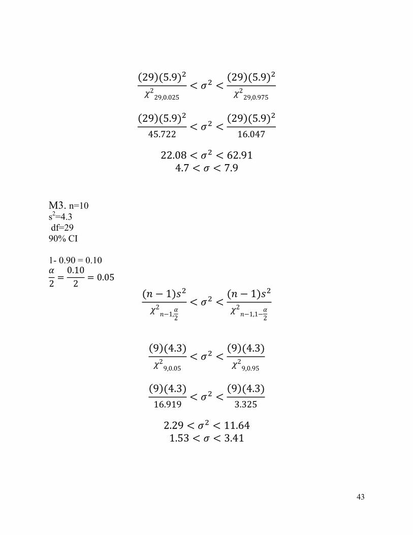
29 5.9229,0.025
29 5.9229,0.975
29 5.945.722
29 5.916.047
22.08 62.91
4.7 7.9 M3. n=10 s2=4.3 df=29 90% CI 1- 0.90 = 0.10
20.102
0.05
12
1,2
12
1,1 2
9 4.329,0.05
9 4.329,0.95
9 4.316.919
9 4.33.325
2.29 11.64 1.53 3.41
44
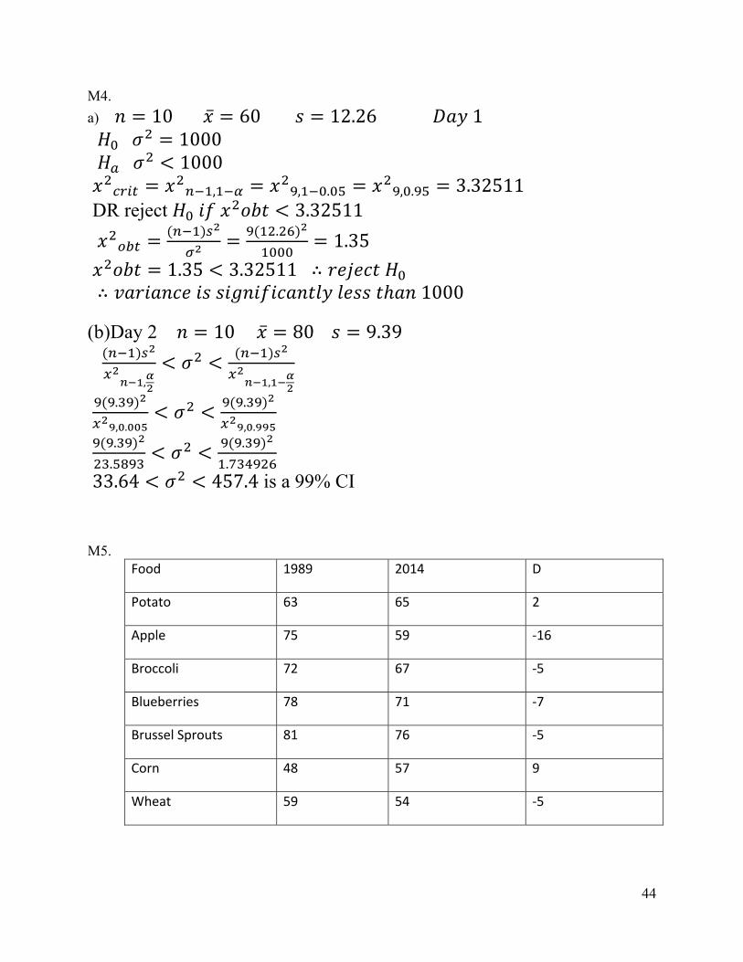
M4.
a) 10 60 12.26 1 1000 1000 , , . , . 3.32511 DR reject 3.32511
. 1.35
1.35 3.32511 ∴ ∴ 1000
(b)Day 2 10 80 9.39
, ,
.
, .
.
, .
.
.
.
.
33.64 457.4 is a 99% CI M5.
Food 1989 2014 D
Potato 63 65 2
Apple 75 59 ‐16
Broccoli 72 67 ‐5
Blueberries 78 71 ‐7
Brussel Sprouts 81 76 ‐5
Corn 48 57 9
Wheat 59 54 ‐5
45
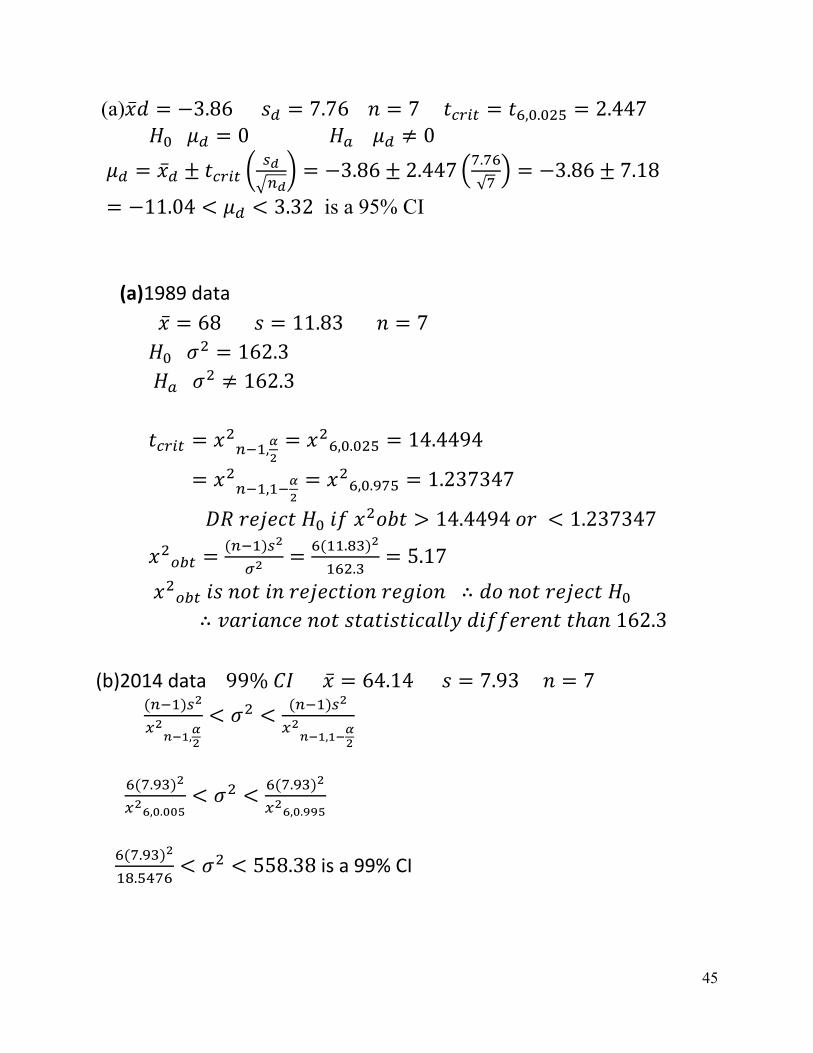
(a) 3.86 7.76 7 , . 2.447 0 0
3.86 2.447 .
√3.86 7.18
11.04 3.32 is a 95% CI
(a) 1989 data
68 11.83 7 162.3 162.3
, , . 14.4494
, , . 1.237347
14.4494 1.237347
.
.5.17
∴
∴ 162.3
(b)2014 data 99% 64.14 7.93 7
, ,
.
, .
.
, .
.
.558.38 is a 99% CI