Stats Lectures - the Department of Statistics

INTRODUCTION TO STATISTICAL MODELLING TRINITY 2002

Linear Models (continued)

Model Checking

After we have fitted a particular linear model to our data set, we can and should perform “model checking.” The first thing we should look at is whether the estimated model is reasonable: specifically, is each estimated parameter value sensible? (e.g., does it make sense that an explanatory variable would have the direction and size of effect on the response that is indicated by its slope?). After checking the reasonability of the model, we need to investigate whether the various assumptions we make when we fit and draw inference using the model are satisfied for our particular data. In addition, we should try to detect the presence of certain other phenomena, such as multicollinearity, that are potential problems for linear models. Lastly, we should check goodness of fit, which is how well the model summarises the relationship between Y and X in our data as measured by how well the response variable is explained/predicted for the data set overall.

If our checks and investigations do reveal that there is a problem with using that

particular model for our data set, then there are a number of different solutions available to us. These solutions range from abandoning that particular linear model in favour of a new one, to adopting different assumptions for our particular linear model (which will probably lead to the use of different estimation and/or inference procedures), to simply using different estimation and/or inference procedures.

Model assumptions

A number of assumptions are made, perhaps implicitly, when we fit and draw inference using a particular linear model. It is important to know what these assumptions are. Further, we should be aware of the potential consequences if an assumption were to break down (i.e., be invalid for our data set). In addition, we should be familiar with techniques, both numerical and graphical, for investigating the validity of the assumptions. Lastly, in the event that a particular assumption does appear to be invalid, it would be useful to know about some alternative models and/or fitting (estimation) and inference procedures that could be used instead of the standard linear model fitted by least squares.

Overview of assumptions 1. Error-free X Assumption: Often, the most commonly forgotten and most difficult to

IAUL & DEPARTMENT OF STATISTICS PAGE 1


understand assumption is the assumption that any error in the linear model has only to do with the response variable and not with the explanatory variables. In other words, it is assumed that the explanatory (dependent) variables are either fixed at certain values or that they are random but can measured without any error. The scenario in which this assumption breaks down and the explanatory variables are random but can only be measured with error (i.e., we observe the value Xi for unit i even though the true explanatory variable value for that unit is actually ηi) is often referred to as errors-in-variables. Often, it is assumed that the errors-in-variables are additive; in other words, the observed value Xi is some function of the true value, ηi, plus an error term. In a simple example of this, the observed and true values of the explanatory variables may be related by the error model

Xi = ηi + δi,

where δi is the error.

When the error-free X assumption breaks down, a potential consequence is that

the estimates of the linear model slopes will be biased. In the case where there is only one explanatory variable, the presence of (additive) errors in that variable will typically bias its slope estimate towards zero (i.e., the estimate will tend to be closer to zero, on average, than the slope’s true value). This phenomena is often referred to as attenuation bias and will lead us to underestimate the effect of the explanatory variable on the response variable. In the case where there is more than one explanatory variable, the effect of errors-in-variables on the estimates of their slopes is less clearcut.

There is really no way to investigate this assumption during model checking.

Sometimes, knowledge about how the data were collected will suggest that there is some error in our Xs and not just in our response variable and lead us to suspect that this assumption is invalid. However, the rest of the time, we typically just assume that this assumption is valid.

If our knowledge does lead us to believe that the error-free X assumption is

invalid, then a variety of solutions present themselves. In one data-based approach, we might keep our standard linear model but try to lessen the effect of the errors-in-variables problem by gathering new data where observations are collected for a very large range of X variable values. The idea is that, in our new data set, the measurement error of the X variables will hopefully be insignificant in comparison with the total variation in the X variables. In an alternative model-based approach, we would stick with our original data set but abandon our standard linear model in favour of a model that incorporates errors-in-variables. Models that incorporate additive errors-in-variables are often termed errors-in-variables models or measurement error models.

2. Correct Specification Assumption: The error term in the model, ε, is assumed to have

mean zero, which is equivalent to saying that the mean of the response variable is, in fact, the specified linear combination of explanatory variables. However, if the



model is not correctly specified (i.e., if the wrong explanatory variables have been included in the linear combination or if the mean response is not a linear function of the specified explanatory variables), then the error terms will not have an expectation of zero. We will refer to the scenario where the errors do not have mean zero as mis-specification or as having an inadequate or incorrectly specified model. In the non-linear instance of mis-specification, the response variable (or, rather, its mean) is not a linear function of the explanatory variables included in our model, but rather some other function: for instance, the mean of the log of the response variable might be a function of these explanatory variables. In the omitted variable instance of mis-specification, our linear model, as specified, does not include an important predictor, which is a variable that does, in fact, have an effect on the response variable even alongside the explanatory variables that are already in the model. This omitted predictor might be a new variable altogether (i.e., an “independent” variable) or, alternatively, some function of the explanatory variables already in the model (e.g., a higher order variable or a product variable). (Here, we should note that mis-specification due to the omission of various higher order and product terms might be thought of as a form of non-linearity).

The consequence of mis-specification is, simply put, that our model misleads us

as to how Y changes with the explanatory variables. For instance, when our linear model omits an important predictor variable, we are not even aware that the response variable is affected by that variable. Also, when our linear model omits a variable or when the form of the relationship between the response and the explanatory variables is actually non-linear, the effects on the response of those explanatory variables that are included in the model are not correctly measured by the values of their respective slopes. For instance, omitting an important variable can result in omitted variable bias: even if a linear relationship is appropriate, when an important predictor is omitted from the linear model, then the estimates of the model slopes for the explanatory variables included in the model will be biased estimates of the true (linear) effect of those variables on the response variable. (Further, the estimate of the conditional (on X) variance of the response variable will be upwardly biased—ie., it will be an overestimate of the amount of variance in Y that is not explained by the Xs.)

Mis-specification due to variable omission can be detected by examining the

estimated conditional variance from the model if a independent estimate of this variance is available from another analysis: a large estimate (relative to the independent estimate) suggests mis-specification. More commonly, though, non-linearity and omission of higher order and interaction terms is detected graphically by looking at plots of the observed residuals versus the predicted Y values and plots of the observed residuals versus each (included) explanatory variable. Further, one should also look at plots of the original Y variable versus each (included and candidate) explanatory variable although, for an independent candidate variable, a partial regression plot may be more useful for detecting mis-specification by omission. (The analysis of plots of residuals versus the included explanatory variables, plots of the observed responses versus each potential explanatory



variable, and partial residual plots for candidate explanatory variables will be addressed when we discuss Model Selection).

If we discover that an important predictor variable, whether independent or a

function of the already included explanatory variables, has been omitted from our linear model, then we will often expand our linear model to include that variable and then refit the expanded linear model to the data. However, deciding whether a particular variable is important enough to be included in the model is not as straightforward as it sounds and will be addressed later when we discuss Model Selection.

If we discover non-linearity in the relationship between the response variable and

explanatory variables (or if we know about it a priori), then we might want to abandon our linear model in favour of a non-linear model (which might be fit by non-linear least squares, for example); this approach is most useful when the relationship between Y and X takes one of a number of frequently used forms. Alternatively, for some particular forms of non-linearity, we might be able to use a linearising transformation where we fit a linear model to a transformed version of the response variable and/or to transformed versions of the explanatory variables. However, even if such a linearising transformation is available, violations of Assumptions 3 and 4 below for our new transformed linear model may lead us to use a non-linear model anyway if we can. However, in certain instances, neither of these approaches may work because we may not be able to specify an exact form (e.g., a specific function) for the relationship between Y and X. In these cases, non-parametric regression techniques (such as loess smoothing) may be a viable alternative: simply put, these regression techniques do not assume that the relationship between Y and X is a straight line but rather estimate the form of that relationship from the data. For example, for our Toyota data set, loess smoothing would draw a curve (not necessarily a smooth one) that describes the relationship between the mean of Mileage and Age through the scatterplot of Mileage vs. Age. If the resulting loess smoothing curve, which would probably have an upward trend but would be somewhat wavy, looks reasonably linear, then we might decide that a linear model is a reasonable enough description of the relationship between the two variables.

3. Normality Assumption: The error term in the model, ε, is assumed to follow a normal

distribution, which is equivalent to saying that the response variable Y has a normal distribution conditional on X (i.e., for each combination of explanatory variable values). The scenario where this assumption breaks down is referred to as non-normality.

In some instances, previous experience or theory may lead us not only to the

belief that the errors will be non-normal, but also to the belief that they will have a specific distribution (other than normal). Alternatively, in other instances, we may simply discover non-normality during model checking and have no idea what the actual distribution of the errors is.



Non-normality does not result in bias in the least squares estimates of the model parameter or standard errors, and the least-squares estimates of the parameters are still the “best” unbiased linear estimates in the sense that they have the smallest variances (provided the other assumptions are met). However, the least squares parameter estimates will do far worse in this sense than various non-linear estimators, even when the errors are only slightly non-normal.

In addition, because normality is needed for tests of significance and confidence

intervals to be valid, non-normality can cause problems with them. More specifically, the p-values for the overall F-test and the t-tests for each model parameter can be incorrect in the case of non-normality. In addition, confidence intervals for the model parameters and, even more so, prediction intervals for particular combinations of X values, can be seriously affected by non-normality, particularly when the distribution of the error terms is highly skewed (i.e., asymmetric). Thankfully, the p-values of significance tests and the confidence intervals for model parameters are not necessarily incorrect just because the errors cannot be assumed to be normal: large sample size can be a coup de grace that restores the validity of our significance tests and confidence intervals. More specifically, even if the error terms are not normal, the sampling distributions of the model parameters will still be approximately normal for large sample sizes according to a version of the Central Limit Theorem. Thus, the p-values for our significance tests and the bounds for our confidence intervals will be okay for large samples since their derivation relies only on the normality of the relevant parameter’s sampling distribution. (For small samples, the error terms must be normally distributed for these sampling distributions to be normal.)

When not expected a priori, non-normality is typically detected using the observed residuals: to do so, one might examine their skewness and kurtosis coefficients (are they close to the normal distribution values of 0 and 3, respectively?), look at a histogram of the residuals (does it look normal?), look at a quantile-normal plot of the residuals (is it close to a straight line?), or perform a Kolmogorov-Smirnoff test for normality (is the null hypothesis of normality not rejected?). Note that it may be very hard to detect slight departures from normality using these techniques, which is a bit worrying since, as stated above, such slight departures can render our least squares estimates far from optimal.

If it appears that the normality assumption is not met, then the typical response

is to try to transform the response variable, Y, so that the resulting model’s residuals are more normally distributed. In certain instances where the error terms are known to have a specific distribution (other than normal), the use of a specific transformation may be called for. However, in other instances, a suitable transformation may be found by trial-and-error. A more sophisticated response to dealing with non-normality is to use a robust regression estimation technique in place of least squares. These estimation procedures are robust to departures from normality in the sense that the parameter estimates they produce do not so quickly become sub-optimal (as do the least squares estimates) when the error distribution departs (moderately) from normality.



4. Constant Variance: The homoscedasticity assumption says that the error term in the

model, ε, has a common or constant variance, σ2. This is equivalent to saying that the conditional (on X) variance of Y is constant or, identically, that the variance of the responses for each combination of explanatory variables is the same. However, one can imagine a number of scenarios in which the variance is not constant; the presence of heterogeneous variances is often referred to as heteroscedasticity. For example, the size of the error term (and thus the size of its variance) might increase with the size of the response; in this instance, the variance would not be the same for all combinations of explanatory variable values since the size of the average response changes (linearly) with the explanatory variables. In another example of heteroscedasticity, the observed response for a particular combination of explanatory variable values in our data set might not correspond to one unit but instead to the average response for several units (that share the same explanatory variable values). In this case, an averaged response pertaining to more units would tend to have a smaller (conditional) variance.

The assumption of constant variance plays an important role in model fitting

(i.e., estimating the parameter values and their errors) in terms of how we weight each observation. We can think of an observation with a smaller (conditional) variance as providing more information about the regression line/plane (or, identically, about its parameters) because its contribution is more certain. Thus, the assumption that the variance is the same for all observations (regardless of their explanatory variable values) means that each observation provides the same amount of information about the parameters and, thus, that each observation should receive the same weight when the linear model is fit to the data. However, if the conditional variance is not constant, then observations with a smaller variance should receive a larger weight when fitting the model to the data.

In some instances, previous experience or theory may tell us that

heteroscedasticity will be present and may also tell us how the conditional variance changes with the explanatory variables or how it differs for each observation in our data set. In other instances, we may simply detect heteroscedasticity during model checking and may have to guess at how the variance changes with the explanatory variables.

Since least squares fitting gives each unit an equal weight, it is reliant on the

validity of the constant variance assumption. Thus, if heteroscedasticity is present, then least squares fitting may not be appropriate: although the parameter estimates it produces will still be unbiased, these estimates may no longer be the “best” (in the sense that they have the smallest variance from the true parameter values) and better estimators might be found. In addition, the constant variance assumption is made when estimating standard errors for the parameter estimates and the conditional variance, when p-values are calculated in tests of significance, and when the bounds of confidence and prediction intervals are calculated; thus, in the presence of heteroscedasticity, the estimates of the conditional variance and the



parameter standard errors are biased, and p-values for significance tests and also confidence and prediction intervals may be incorrect.

When not expected a priori, heteroscedasticity is typically detected using the observed residuals: plots of these residuals versus the predicted values or versus each explanatory variable are particularly useful for doing so. Whether expected a priori or discovered during model checking, the presence of heteroscedasticity is typically dealt with using two approaches. One is to fit the model using Generalized Least Squares (or, more specifically, a special case of GLS referred to as Weighted Least Squares) rather than with ordinary least squares; this approach is most useful when it is known how the variance changes with the explanatory variables or how it differs for the observations in the data set. The other approach is to try to find a transformation of the response variable that eliminates heteroscedasticity.

5. Independence: The error terms or, equivalently, the responses, are assumed to be independent of each other (in a statistical sense). The scenario in which this assumption breaks down is often referred to as having correlated errors or responses.

The independence assumption is often violated when some of the observations

in the data set are related to each other in the sense that they can be conceptually grouped together. For instance, the observations might be units that belong to larger groups (e.g., the data set contains information on a number of students from each of several schools), or there might be multiple observations per unit (e.g., the outcome variable is measured numerous times for each unit). In some instances, the grouping of observations is part of the design of the study or of the resulting data set (e.g., blocking was used in an experiment and there are several observations for each block); in these instances, the presence of higher level groups is obvious and, thus, so is the possibility that the responses within these groups might depend on each other. However, in other instances, a higher level grouping and a potential for correlated responses might be introduced inadvertently, such as when experimental units are grouped for convenience when exposing them to treatments or taking their measurements.

Alternatively, the independence assumption may also be violated because time

played a role in the performance of the study (e.g., a chemical solution whose effect lessens over time is applied to units one by one) or in the collection of data (e.g., the units are weighed one by one and the scale is only tared at the beginning). When time plays a role, the error (or response) associated with an observation at one time point will tend to be correlated with the errors (or responses) of the immediately preceding observations. The presence of correlation between responses and errors due to the effect of time is often referred to as serial correlation. Sometimes, it will be clear from the study design or data collection method that the observations can be ordered in a time sequence and that serial correlation may be present. Other



times, however, the presence of serial correlation can be far more subtle and difficult to detect.

Saying that the errors are positively correlated means that, with grouping error,

two members of the same group are likely to both have big errors or both have small errors or, with serial correlation, a big (small) error for one observation means that the subsequent observation (in terms of time) is likely to have a large (small) error as well.

The potential consequences when the independence assumption breaks down

are similar to the possible effects of the presence of heteroscedasticity (see 4. above). As stated above, it is sometimes very obvious from the nature of the study or the

data that the errors (and responses) are probably correlated, whether due to grouping or to a time effect. In other instances, however, the breakdown of the independence assumption may have to be detected during model checking by examining the standard errors and variances (inordinately small ones can be a sign of correlation) or, in the case of serial correlation, by plotting the residuals according to the order in which the data was collected, the treatment was administered, etc . . . ., and looking for a trend.

If correlation is present, then two approaches present themselves. For instance,

one could fit the linear model using Generalized Least Squares, which takes the correlation structure of the data set into account. Alternatively, one might use a model that is more appropriate for the particular nature of the data: for grouped data, a fixed effects, random effects, or mixed effects model could be used, or, if the data has a time effect, a model with a time series component could be used.

Graphical techniques for checking assumptions Residuals

Many of the graphical techniques available to us for trying to detect problems with the correct specification, normality, constant variance, and independence assumptions entail using the n residual values since these values can be thought of as estimates of the error terms. Here, we recall that the (raw) residual for observation i, which we will call ei, is the difference between observation i’s observed Y value and the Y value that the model predicts for observation i:

)ˆˆˆˆ(ˆ

,,22,110 ippiiiiii XXXYYYe ββββ ++++−=−= L . Using this definition, we can calculate n residuals, one associated with each observation in the data set. We should note that because of the way in which the eis are calculated, they do not have a common variance and they are correlated with each other; we reiterate that this is merely an artefact of the way in which the residuals are



calculated and is true regardless of whether the constant variance and independence assumptions about the true errors, the εis, are valid.

As just stated above, the raw residuals, as calculated, do not have a common variance: in fact, the variance of the residual term is smaller for observations with more extreme explanatory variable values (e.g., the Toyota Aged 15 years in our previous Toyota example). Thus, we may want to standardise the raw residuals by dividing each residual by its estimated standard error (the square root of its estimated variance) because doing so will give all residuals a common variance and put them on the same scale. The resulting standardized residuals (or, as they are known to some, the internally studentized residuals) are denoted by ri or by ei’ and are calculated using the equation

ii

i

ii

iiii h

eYYesYYer

−=

−

−==

1ˆ)ˆ(ˆ

ˆ'

σ,

where the denominator is the square root of the estimated variance of the ith raw residual. Here, is the estimated residual standard error (introduced previously), and h

σii is the leverage for observation i. Leverage will be discussed in greater detail later

but, essentially, is a measure of how (relatively) extreme the explanatory variable values are for a particular observation: hii is close to 1/n for observations with very typical explanatory variable values and close to 1 for observations with very extreme explanatory variable values. The n standardized residuals all have a common variance of 1 (but are still correlated with each other) and, thus, we may prefer to use the standardized residuals when checking linear model assumptions 2 – 5. However, instead of using either the raw or standardised residuals for model checking, it may be even better to use yet another type of residuals: the studentized residuals, which are also known as externally studentized residuals, jackknife residuals or deletion residuals. The studentized residual is motivated by the notion that looking at the difference Y may give us an overly optimistic view of how good the model is at predicting response values: more specifically, since Y is a prediction from the linear model fitted to a data set that includes observation i, we would expect that it should give a pretty good prediction of the response for unit i. However, what if we were to delete observation i from the data set, fit the model (i.e., estimate its parameters) using this new data set, and then calculate the predicted value for observation i under this new model? We will use Y to refer to the prediction of the response for observation i from the model fitted to the data with observation i deleted. Since this prediction comes from a model whose fit is in no way specific to observation i (in the sense that the model parameters were estimated from a data set without observation i), the difference between the actual response for observation i and Y should give us a pretty realistic view of how good the model is at predicting a response (for observation i). The studentized residual, or , looks at this distance, Y , or, rather, at a standardized version of it:

ii Y−

i

)(i

*ir

)(i

ˆi Y−*

ie )(i



)ˆ(ˆ

ˆ

)(

)(**

ii

iiii YYes

YYre

−

−== .

Regardless of whether one decides to use the raw, standardized, or studentized residuals for model checking, most methods of investigating the linear model assumptions using the residuals are graphical and involve plotting these residuals. Below, we discuss several particularly useful diagnostic plots (plots used to diagnose departures from the assumptions made when fitting the model and to detect poor fit). Scatterplot of residuals versus predicted values

This plot of (or eie i’) versus Y can be used to detect problems with the constant variance assumption and, to some extent, the correct specification and independence assumptions; checking these assumptions essentially entails looking for patterns between the (predicted) response variable and the estimated errors or residuals. If the linear model assumptions are satisfied, then you will most likely see no patterns in this plot: basically, you hope that the points in this plot will be randomly scattered around 0. However, you might look for and find patterns in the magnitude of the residuals, which can indicate heteroscedasticity (i.e., the breakdown of the constant variance assumption). For example, if the size (whether positive or negative) of the residuals increases as the predicted value increases, which will show up in the plot as a fan-shaped pattern with the fan opening to the right, then you may suspect that the variance of the errors (as portrayed by the variance of the residuals) is non-constant. Alternatively, you might look for and find patterns in the residuals themselves rather than in their magnitude: such a trend would suggest that the model, as estimated from the data, is not a good description of the relationship between the explanatory variables and the response variable. Such a trend may suggest that the estimated model is inadequate for the data because the model itself is mis-specified; hence, trends in the residuals can be an indication that the correct specification assumption has been violated. For example, if there is a curved trend in the residuals, you might suspect that the relationship between the response and explanatory variables is actually non-linear. Alternatively, however, a trend in the residuals could result from a problem with the estimation of the model’s parameters rather than a problem with the model’s specification: a linear trend might result from the presence of an influential point that has greatly affected the estimates of the model parameters and made the model a worse fit for most other points. (Influential points will be discussed below.) Lastly, a pattern in the residuals might indicate problems with the independence assumption, such as serial correlation: for example, a pattern in the residuals could result from the presence of a time effect in the data, as is the case with the Ben Johnson – Carl Lewis split time data examined in lecture.

i

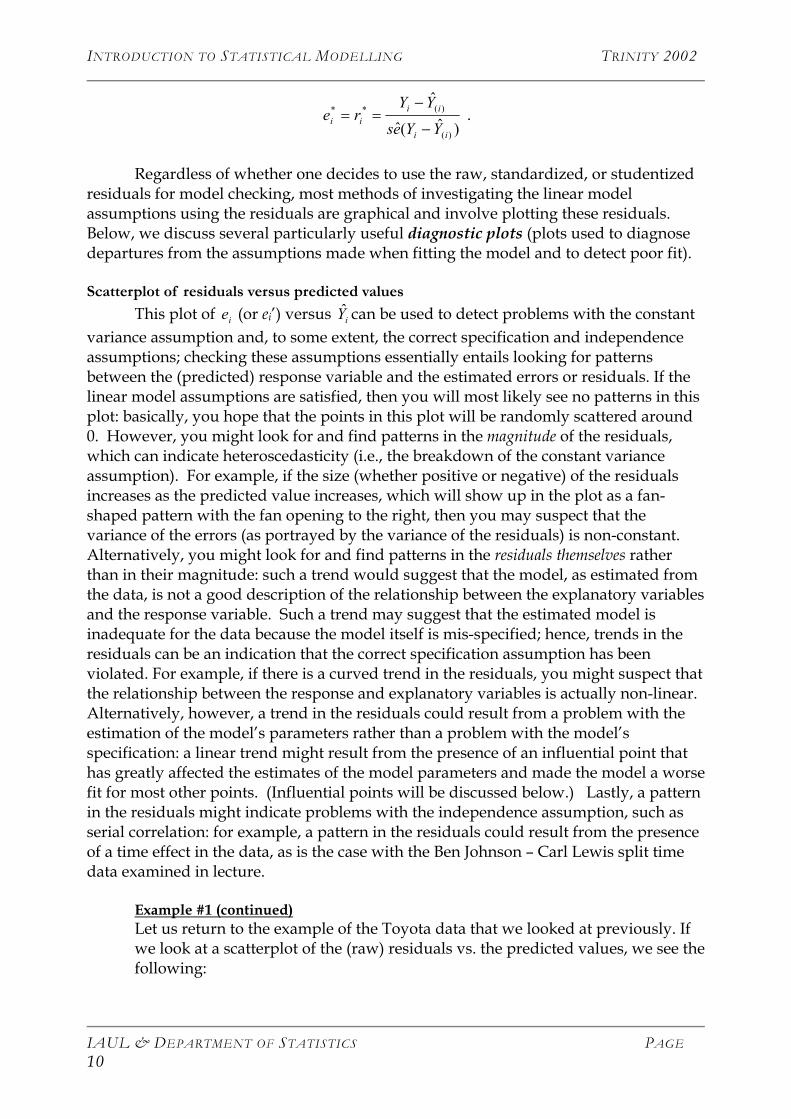
Example #1 (continued) Let us return to the example of the Toyota data that we looked at previously. If we look at a scatterplot of the (raw) residuals vs. the predicted values, we see the following:



•

•

•

•

•

•

•

•

•

•

•

Fitted : sdo.age

Res

idua

ls

75 80 85 90 95

-60

-40

-20

020

8 10

11

Figure 1: Scatterplot of raw residuals versus predicted values for the Toyota data

Looking at this plot, we note that there are a number of problems with the model we fitted. First, if we look at the size of the residuals, we note that one of the observations, 11, has a very large negative residual and is wrongly predicted by around 60,000 miles: the model does not seem particularly appropriate for point 11. Second, if observation 11 is ignored, there appears to be a linear relationship between the fitted value and the residual: in fact, this linear trend in the majority of the residuals is yet another reflection of the fact that the model does not fit observation 11 well, a subtlety which we will understand better later when we discuss influential observations ■

Scatterplot of observed response variable versus predicted values

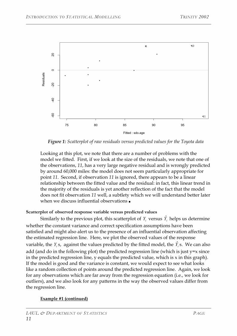
Similarly to the previous plot, this scatterplot of Y versus Y helps us determine whether the constant variance and correct specification assumptions have been satisfied and might also alert us to the presence of an influential observation affecting the estimated regression line. Here, we plot the observed values of the response variable, the Y s, against the values predicted by the fitted model, the Y s. We can also add (and do in the following plot) the predicted regression line (which is just y=x since in the predicted regression line, y equals the predicted value, which is x in this graph). If the model is good and the variance is constant, we would expect to see what looks like a random collection of points around the predicted regression line. Again, we look for any observations which are far away from the regression equation (i.e., we look for outliers), and we also look for any patterns in the way the observed values differ from the regression line.

i i

i i

Example #1 (continued)



For the Toyota data, we obtain the following Y versus Y scatterplot: i i

•

•

•

•

•

••

•

•

•

•

Fitted : sdo.age

sdo.

mile

age

75 80 85 90 95

4060

8010

012

0

Figure 2: Scatterplot of observed responses versus predicted values for the Toyota data

Again, we note that, with the exception of observation 11, there appears to be a strong pattern (as the fitted values increase) in the departure of the observed values from the predicted regression line: as did the previous plot, this suggests that the model we have fitted to our data is not an accurate description of the trend seen in the data set. We can also clearly see that there are large deviations from the predicted regression line for certain points, such as 11 ■

Normal probability plot of the residuals

The third plot that we consider for use in checking whether we have satisfied the assumptions is something called a normal probability plot or a quantile-normal plot of the residuals. This plot is used to check the normality assumption since it allows us to investigate whether the residuals are normally distributed: since the residuals can be thought of as estimates of the errors, evidence that the residuals are non-normal might lead us to suspect that the errors are not normal. A normal probability plot is based on the idea that the proportion of (standardized) residual values less than a specific value should be approximately equal to the probability that a N(0,1) random variable is less than the same specific value. However, you do not need to worry too much about the theory behind quantile-normal plots since most software packages produce these plots (sometimes called either PP or QQ plots). Instead, you should concentrate on their interpretation: what you hope to see (and would see if the residuals are normally distributed) is a trail of points that closely follows a straight line. However, even if the residuals are normal, the trail of points may deviate a bit from this line at either end. Thus, we are primarily interested in detecting large deviations (or patterned



deviations) from the line. If the points do not appear to follow the straight line, then you must suspect that the errors are probably not normally distributed.

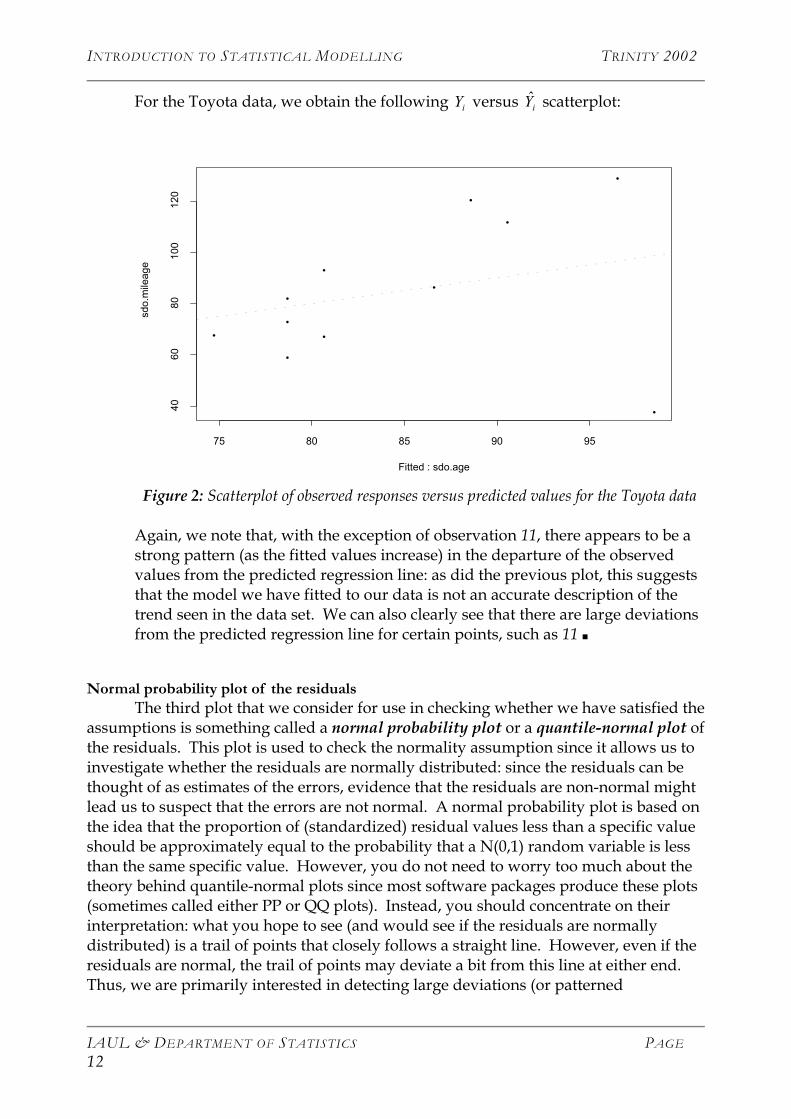
Example #1 (continued) For the Toyota data, we get the following quantile-normal plot for the (raw) residuals.

•

•

•

•

•

•

•

•

•

•

•

Quantiles of Standard Normal

Res

idua

ls

-1 0 1

-60

-40

-20

020

8 10

11

Figure 3: Quantile-normal plot of the raw residuals for the Toyota data

In this plot, there appears to be a general pattern in which the residuals snake about the line, and there are also a number of large deviations from the straight line. Thus, this plot suggests that we may have violated the normality assumption that we made when we fitted a linear model to this data ■

Residual plots for detecting serial correlation

In order to detect serial correlation, one would first order the observations according to the suspected time component (whether it corresponds to the time at which their treatments were administered, the time at which their variables were measured, etc . . . .).

Then, one might make an index plot of the residuals in which each residual value is plotted against its order number. This index plot, which is essentially a times series plot, can then be examined to determine whether there is either positive or negative correlation present in the ordered residuals. However, since it can be difficult for those unfamiliar with the analysis of times series to detect correlation in an index plot, it may be better to make a scatterplot in which every residual (except the first one in



order) is plotted against the preceding residual (in the time ordering). Any positive serial correlation in the residuals will show up as an upwardly sloping trend in this plot of ei versus ei-1; similarly, any negative serial correlation will show up as a downward sloping trend.

Some potential solutions when assumptions 2 – 5 break down Transformations

As stated above, transformations of the response variable can be useful tools for dealing with the problems of heteroscedasticity and non-normality, and transformations of the response variable and/or the explanatory variables can be used to address mis-specification because of non-linearity. However, it is often the case that a particular transformation will solve one problem while perhaps leaving the other problems worsened or unchanged. For instance, a logarithmic transformation of Y may linearise the relationship between Y and X; however, unless the original error terms (belonging to the linear model that predicted Y) were multiplicative (multiplied X rather than being added to it) and had a log-normal distribution, then the resulting error terms (belonging to the linear model that predicts log(Y) ) will not have a normal distribution with constant variance as desired.

Transforming the variables using particular transformation (say, f() for Y and g() for X1 ) entails first creating new variables in the data set (say Yt and ) by applying f() to the response variable value and g() to the explanatory variable value for every observation in the data set:

tX 1

)( iti YfY = and for i = 1, . . ., n. )( i

ti XgX =

The original linear model

pp XXXXYE ββββ ++++= L22110]|[

is then applied to the newly created response variable and to the newly created explanatory variable with all the non-transformed explanatory variables left the same:

ptp

tttp

tp

ttttt XXXgXXXXYfEXYE ββββββββ ++++=++++== LL 2211022110 )(]|)([]|[

This new linear model is fitted to the data set containing Yt, , XtX 1 2, . . . ., and Xp. In the above, it is important to note that the parameters of the new linear model (the βts) and the original linear model (the βs) are not the same in the sense that they do not describe the same aspect of the relationship between Y and X (and, thus, will not have the same values). This is true even for regression slopes pertaining to explanatory variables that have not been transformed; the interpretation (and value) of these parameters are different in the original and new models because the response variable has been transformed.



However, when we are using a transformed model and explanation is our goal, we are often not actually interested in the parameters of the new linear model (the βts); this may be the case because we want to quantify the effect of the original (untransformed) X variables on the original Y variable or because our new model is a linearisation of a non-linear model whose parameters have an interesting interpretation (an example of this will be given below). In these cases, we may be more interested in some re-transformation of the βts: if this is the case, the usual procedure is to estimate the βts and form confidence intervals for them and then to retransform the upper and lower bounds of the confidence intervals. As an example, suppose that the new linear model is in terms of the logarithm of the response variable:

110]|)[log( XXYE tt ββ += .

In the above model, describes how an increase of 1 unit in Xt1β 1 effects the mean of

log(Y): more specifically, it tells us how much is added to (subtracted from) log(Y) when X1 increases by 1. However, what if we are truly interested in the effect of X1 on the original response variable, Y? Well, as some basic mathematics can show, a re-transformed version of , namely exp( ), describes how an increase of 1 unit in Xt

1βt1β 1

effects (the median of) Y: specifically, it tells us what factor Y is multiplied by when when X1 increases by 1. We are more interested in exp( ) than in : thus, we estimate and make a confidence interval for it using the typical techniques with the above linear model, but then we apply exp() to the lower and upper bounds of the confidence intervals in order to make it relevant to exp( ).

t1β

t1β

t1β

t1β

Similarly, when we are using a transformed model and prediction is our goal, we may not be interested in predicting the transformed version of the response variable but may want to predict the response variable in its original form. If this is the case, we can calculate an estimated prediction and a prediction interval for the transformed response using our new linear model and then re-transform the bounds of the prediction interval in order to make it relevant for the original response variable. For instance, in the above example, for a specific X1 value, we would estimate a predicted value and find a prediction interval for log(Y) using the new linear model, but would then apply exp( ) to the lower and upper bounds of the interval in order to put it in terms of Y.

Sometimes, the particular transformation of Y and/or X that will solve the problem(s) at hand will be known a priori as a result of previous experience or theory. As an example, in certain scientific applications, we might know that the relationship between Y and X takes the form:

110αα XY ⋅= .

We could fit the above non-linear model to the data using a technique such as non-linear least squares. However, it might be more convenient to simply fit a linear model to transformed versions of the variables. More specifically, if we take the logarithm of



both sides of the above equation, it gives us the linear equation

)log()log()log( 110 XY αα += .

We can rename log(α0) as β0 and α1 as β1 giving us

)log()log( 110 XY ββ += ,

which is just a linear model in terms of log(Y) and log(X1). Thus, we might transform both Y and X1 using a logarithmic transformation and then fit a linear model to the transformed variables. Here, it is important to note that, if we are interested in the parameters of the original non-linear model (i.e., α0 and α1), then we will have to re-transform the confidence interval bounds for β0 using exp( ) in order to make the interval relevant for α0.

Other times, however, this will not be the case, and the data analyst will have to find the “best” transformation of Y and/or X (the transformation that minimises the problems of heteroscedasticity, non-normality, and/or non-linearity as much as possible). The best transformation may be found by exploration; this entails, for various different transformations of the response and/or explanatory variables, fitting the model to the transformed data and then looking at various statistics and graphical plots to see whether the heteroscedasticiy, non-normality, and non-linearity are present. Some particularly useful transformations to try are log() and square root(): not only do these transformations often seem to solve the aforementioned problems, but the parameters of the resulting models can often be easily re-transformed to describe the relationship between Y and X in their original form. Alternatively, instead of using exploration, the best transformation could be found by using some sort of transformation-seeking algorithm (e.g., Box-Cox, Box-Tidwell). For example, the Box-Cox procedure seeks the power transformation of the response variable (e.g., Y3, Y2, Y, Y1/2= Y , log(Y), Y-1= 1/Y) that best satisfies the assumptions that the error terms have a N(0,σ2) distribution.

For an excellent discussion of using transformations to correct heteroscedasticity, non-normality, and/or non-linearity, please see Chapter 11 of Rawlings, J. (1988), Applied Regression Analysis: A Research Tool.

Generalized Least Squares (Weighted Least Squares) Generalized Least Squares (GLS) is a fitting method that can be used instead of

Least Squares to estimate the parameters of our linear model and their standard errors when we are not comfortable making the assumptions of constant variance and independence. As stated above, the least squares estimates of the parameters are only the best (in the sense that they vary the least from the true values of these parameters) when these assumptions are satisfied. Further, the usual estimates of the parameter standard errors are only unbiased (for the true standard errors) when these assumptions are valid. However, when the constant variance and independence assumptions are not valid but we are able to specify how the conditional variance



differs for the observations in the data set and how they are correlated with each other, then GLS produces estimates of the linear model parameters that are the “best” and estimates of their standard errors that are unbiased. This said, GLS fitting is not a panacea: it only performs well in the sense described above when the form of the correlation between observations and the way in which their conditional variances differ is known from theory, previous experience, or knowledge about the data itself. In most instances, it is pretty unlikely that we will know these things, and, thus, we would have to use the data to guess at or estimate the form of the correlation and variance structure of the observations. In these cases, GLS would no longer be optimal in the sense described above; in fact, it might be even worse than just using ordinary least squares to estimate the model parameters and their standard errors.

As a note, Weighted Least Squares (WLS) is a special case of GLS for when we are still willing to assume that the observations are independent of each other but do not feel comfortable making the constant variance assumption because of prior knowledge or because of discoveries we made when checking our linear model. In WLS, we do not need to specify a correlation structure for the observations (because WLS assumes that they are independent) but we do need to specify how the conditional variance for the observations varies. For example, suppose we have a data set where each observation corresponds to a number of units (i.e., the response variable value is the average response for several units that all share the same explanatory variable values). Well, in that case, we might specify that an observation’s conditional variance is proportional to 1 over the square root of the number of units it corresponds to (recall that the standard error of the sample mean is in/σ for a sample of ni units). When WLS estimates the model parameters and their standard errors, each observation is given a weight that is inversely proportional to its specified conditional variance: in other words, observations with smaller specified conditional variances are given a bigger weight when the linear model is fit by WLS.

Other potential problems with linear models

Multicollinearity Multicollinearity is a problem that potentially occurs only when you have more

than one explanatory variable. Simply put, multicollinearity means that some of the explanatory variables are highly related to each other, making it very difficult to distinguish the separate effects of these explanatory variables on the response variable. This is a problem because our linear model, by including a separate term for each explanatory variable with its own parameter, requires that the individual effect of each explanatory variable on the response variable be estimated. As an example of multicollinearity, suppose that we are investigating the relationship between people’s height, weight, and body mass index (weight/height^2) and their effect on cholesterol levels. Clearly, weight, height and body mass index are highly correlated with each



other, and, thus, we might worry about multicollinearity. The main consequence of multicollinearity for our linear model is that the

estimates of the individual parameters tend to be highly uncertain as reflected by the fact that their estimated standard errors and, as a result, their p-values, are extremely large. If the goal of fitting a linear model is explanation, meaning that we are ultimately interested in the model parameters since they quantify the effect of the explanatory variables on the response variable, then this consequence can be a very serious one: the presence of multicollinearity can seriously damage our efforts to determine which explanatory variables are important and to measure the effect each has on the response variable. However, if our goal is prediction, then the consequences of multicollinearity are less severe: as long as the model fits the data well overall and as long as the observations whose Y values we will be predicting will also have this same pattern of multicollinearity among their X variables, then we should be okay.

One can actually check for multicollinearity before fitting the model to the data. The easiest way to do this is to examine the correlations between each pair of explanatory variables. If two of the variables are highly correlated (e.g., they have a correlation less than -0.60 or greater than 0.60), then multicollinearity may be a problem. The correlation approach can only detect when pairs of variables are highly (linearly) related. However, the form of multicollinearity can be much more complicated, involving a relationship between three or more variables, and, thus, will not necessarily be detected by the correlation approach. For this reason, multicollinearity is often looked for before fitting the model by examining the singular values of the matrix of explanatory variables (with a column for the constant or intercept term); however, this approach to detecting collinearity is beyond the scope of this course and will not be discussed here. Multicollinearity can also be detected after the model has been fitted to the data by looking at the output for the linear regression. Very unreasonable estimates or extremely large estimated standard errors for some slope parameters can be an indication that multicollinearity is present. Additionally, if the linear model seems to fit the data well overall (e.g., the null hypothesis of no effect is rejected in the F-test for overall significance or, identically, R2 is high) , but most of the explanatory variables are not significant according to their p-values, then multicollinearity might be the cause.

Once multicollinearity has been detected, what do we do about it? There are a number of possibilities. A simple approach for the case in which multicollinearity is caused by one or more pairs of highly correlated explanatory variables is to simply remove one of the variables from each pair; this process can continue until we have a model with no pairs of variables that are highly correlated. However, as stated previously, the multicollinear relationship between explanatory variables can often be very complex in nature, therefore not lending itself to this simple approach. If this is the case, then a fairly sophisticated solution would be to use one of the biased regression techniques such as ridge regression or principal components regression; these



regression techniques produce (biased) parameter estimates that are typically smaller in magnitude than the corresponding least squares estimates. The idea behind these biased estimation techniques is that, by relaxing the constraint that the estimates of the parameters must be unbiased, one might end up with estimates that vary less (from the true parameter values) than the standard least squares estimates (which are only the best or least variable out of the set of unbiased estimators.)



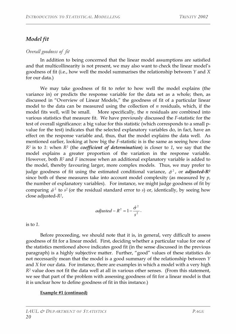
Model fit

Overall goodness of fit In addition to being concerned that the linear model assumptions are satisfied

and that multicollinearity is not present, we may also want to check the linear model’s goodness of fit (i.e., how well the model summarises the relationship between Y and X for our data.)

We may take goodness of fit to refer to how well the model explains (the variance in) or predicts the response variable for the data set as a whole; then, as discussed in “Overview of Linear Models,” the goodness of fit of a particular linear model to the data can be measured using the collection of n residuals, which, if the model fits well, will be small. More specifically, the n residuals are combined into various statistics that measure fit. We have previously discussed the F-statistic for the test of overall significance: a big value for this statistic (which corresponds to a small p-value for the test) indicates that the selected explanatory variables do, in fact, have an effect on the response variable and, thus, that the model explains the data well. As mentioned earlier, looking at how big the F-statistic is is the same as seeing how close R2 is to 1: when R2 (the coefficient of determination) is closer to 1, we say that the model explains a greater proportion of the variation in the response variable. However, both R2 and F increase when an additional explanatory variable is added to the model, thereby favouring larger, more complex models. Thus, we may prefer to judge goodness of fit using the estimated conditional variance, , or adjusted-R2σ 2

since both of these measures take into account model complexity (as measured by p, the number of explanatory variables). For instance, we might judge goodness of fit by comparing 2σ to s2 (or the residual standard error to s) or, identically, by seeing how close adjusted-R2,

2

22 ˆ1

sRadjusted σ

−=− .

is to 1.

Before proceeding, we should note that it is, in general, very difficult to assess goodness of fit for a linear model. First, deciding whether a particular value for one of the statistics mentioned above indicates good fit (in the sense discussed in the previous paragraph) is a highly subjective matter. Further, “good” values of these statistics do not necessarily mean that the model is a good summary of the relationship between Y and X for our data. For instance, there are examples in which a model with a very high R2 value does not fit the data well at all in various other senses. (From this statement, we see that part of the problem with assessing goodness of fit for a linear model is that it is unclear how to define goodness of fit in this instance.)

Example #1 (continued)



For our Toyota model, R2 = 0.08152

which means that only 8% of the variation in Mileage has been explained by fitting a linear model. This tells us that the model that we have fitted is useless. Not only does it fail to satisfy the assumptions used to fit it (as seen in our previous examination of diagnostic plots), but it doesn’t explain much of the variation in the data set ■

Poor overall fit, as measured by the aforementioned statistics, might occur because the model isn’t actually good at predicting/explaining Y for the data as a whole. If this is the cause of the poor fit, then we might want to abandon the linear model in favour of a different one (e.g., a linear model containing a different set of explanatory variables, a linear model in which the response and/or some of the explanatory variables have been transformed, or perhaps even a non-linear model.) This approach is essentially an exercise in Model Selection, which we will discuss later. However, before proceeding, it is important to note that poor overall fit (as measured by the previously mentioned statistics) might also occur because the linear model is not a good fit (in this sense) to a small number of observations, even if the model is a good fit for the vast majority of the data. To see whether a few observations are causing the poor overall fit, we need to search for outlying observations, which we will now discuss!

Fit for individual observations (cases) – a discussion of outliers If the values of the statistics mentioned above indicate that the model fits the

data poorly (in some sense), we might be interested in finding out whether the poor fit is being caused by a particular observation (or observations), which can be assessed by looking at the size of its residual. We will use the term residual outliers to refer to observations that are not well fit by the linear model as estimated (i.e., observations with large negative or large positive residual values). For example, in the Toyota data set, the Toyota Aged 15 years has a large negative residual and is thus a residual outlier. To locate residual outliers, we might look at a scatterplot of the standardized residuals against the predicted values ( versus Y ) and mark as a residual outlier any observation with a particularly extreme residual (say below –2 or above +2).

'ie i

However, we might be more interested in detecting linear outliers, which are observations that do not adhere to the linear trend exhibited by the majority of the observations. These observations may be of interest for their own sake since they are anomalous and thus may make interesting case studies. In addition, they may also be of interest because they can affect our conclusions about the general effect of the explanatory variables on the response (for all those observations that do follow the majority linear trend) and about the overall goodness of fit of the model.

Detecting linear outliers is easy enough when there is one explanatory variable

(as with the Toyota data): we can just look at a scatterplot of the response variable



against the explanatory variable and see if any points do not fit in with the general linear trend of the data. For example, in the Toyota data, we have one observation (in the lower right corner) which has a very low mileage compared to what we would expect from the rest of the data; thus, this observation is not only a residual outlier but also a linear outlier. With more than one explanatory variable, this approach cannot be used to detect linear outliers and we will often try to use the residuals to do so by noting large positive or negative residual values.

Yet there is a problem with using the magnitude of the residuals to locate linear

outliers: simply put, residual outliers are not necessarily linear outliers, and vice versa. The crux of this problem is the existence of influential observations. An influential observation is one that (considerably) affects the estimates of the linear model parameters or, identically, (considerably) affects the choice of the best fitting line/plane for the data. Essentially, an influential observation does not follow the general linear trend of the data and pulls the estimated line/plane towards itself in order to minimise the distance between its actual response and the predicted response on the line/plane. As a result, that observation’s calculated residual value may be small, and, so, just looking at the standardized residual for that point would not reveal that it is a linear outlier. Also, because this high influence observation pulls the line/plane away from other observations, those observations may end up with large residuals and appear to be linear outliers even though they actual follow the general linear trend of the data. This phenomenon is, in fact, what happens in our Toyota data example: the observation in the lower right corner (for the fifteen year old Toyota) is influential and pulls the regression line towards itself. The result is that its residual is smaller than it would be if we were to draw in the line that best fit the other 10 points, although its residual is still negative enough for us to note it above. The other result is that the regression line is pulled away from the other 10 points, giving them bigger residuals (than they would have if we were to draw in the line that best fit them) and creating a linear trend in the residuals (as seen in the above plot of versus Y ). ie i

Thus, when looking for linear outliers, we need to look at case statistics (i.e.,

statistics that are calculated for each observation in the data set rather than for the data set as a whole) other than just the raw and standardized residuals.

We might first consider checking the leverage, hii, for each observation to see

whether it is large because an observation with high leverage has the potential to influence or change the model’s parameter estimates (and the location of the best fitting line/plane) considerably. As stated before, leverage is a measure of the extremity of an observation’s X values. We should note that leverage looks at extremity in terms of all the explanatory variables together. For instance, if we have three explanatory variables, we can think of plotting them in 3D space, which will result in a cloud of points: observations near the middle of this cloud have smaller leverages, and observations near its edges have higher leverages. This idea that leverage looks at extremity in terms of all the explanatory variables together is an important one: one observation might not have an extreme value for any of the explanatory variables taken one at a time, but still might be considered to have extreme X values (i.e., high



leverage) when they are all considered together. How do we decide whether or not a particular observation has high leverage? It is common practice to say that an observation has high leverage if its hii value is above 2p/n (or, sometimes, 3p/n). (Note that hii falls between 1/n and 1 by definition, and that the average of the hiis for all n points is p/n.) And what does it mean if a particular observation has high leverage? Well, it means that this observation has only the potential to influence or change the model’s parameter estimates (and, thus, the estimated best fitting line). A high leverage observation will actually be influential only if it is also a linear outlier: if the observation does follow the general linear trend of the data, then it will not need to realise this potential of influencing the estimated regression line. When a high leverage observation is a linear outlier, then it will influence the parameter estimates and the resulting estimated line quite a bit; in this case, the observation could end up with a small (standardized) residual because it has pulled the line/plane towards it, thereby obscuring the fact that it is a linear outlier. The bottom line is as follows: if we find that an observation has a high leverage value, then we should be alerted to the possibility that it might be an linear outlier even if its (standardized) residual value is small.

A second case statistic we might want to look at is Cook's distance, which is a measure of influence. The details of calculating Cook’s distance are not given here, but most statistical packages allow us to produce a plot of the Cook's distance for each observation. Let us simply note that the Cook’s distance for observation i essentially tells us how much the estimates of the linear model parameters (and thus the estimated line) would change if that observation were left out of the data set (if they change a lot, then the point is influential). The scale on which Cook's distance is measured is not important: all you have to remember is that, the higher the Cook's distance, the more influential the observation is in calculating the estimates of the regression coefficients. Some statisticians use a cut-off of 0.8-1.0, marking as influential any observations with Cook’s distances above this range. In general, an observation cannot considerably affect the parameter estimates if it follows the general linear trend of the data: thus, it will generally be okay to consider points with large Cook’s distances as linear outliers. However, as we will note in the follow example, this is not always strictly true since an observation that is not a linear outlier can have a large Cook’s distance because of the presence of another observation that is actually a linear outlier. Is the opposite true: can we conclude that points with small Cook’s distances are not linear outliers? The answer here is unfortunately no. For instance, if there are two linear outliers that share the same data values, the Cook’s distance for each of them might still be small because Cook’s distance looks at the effect on the parameters of removing only one observation at a time from the data set (and the other linear outlier would still be in the data set, keeping the parameter estimates from changing and the line/plane from moving).

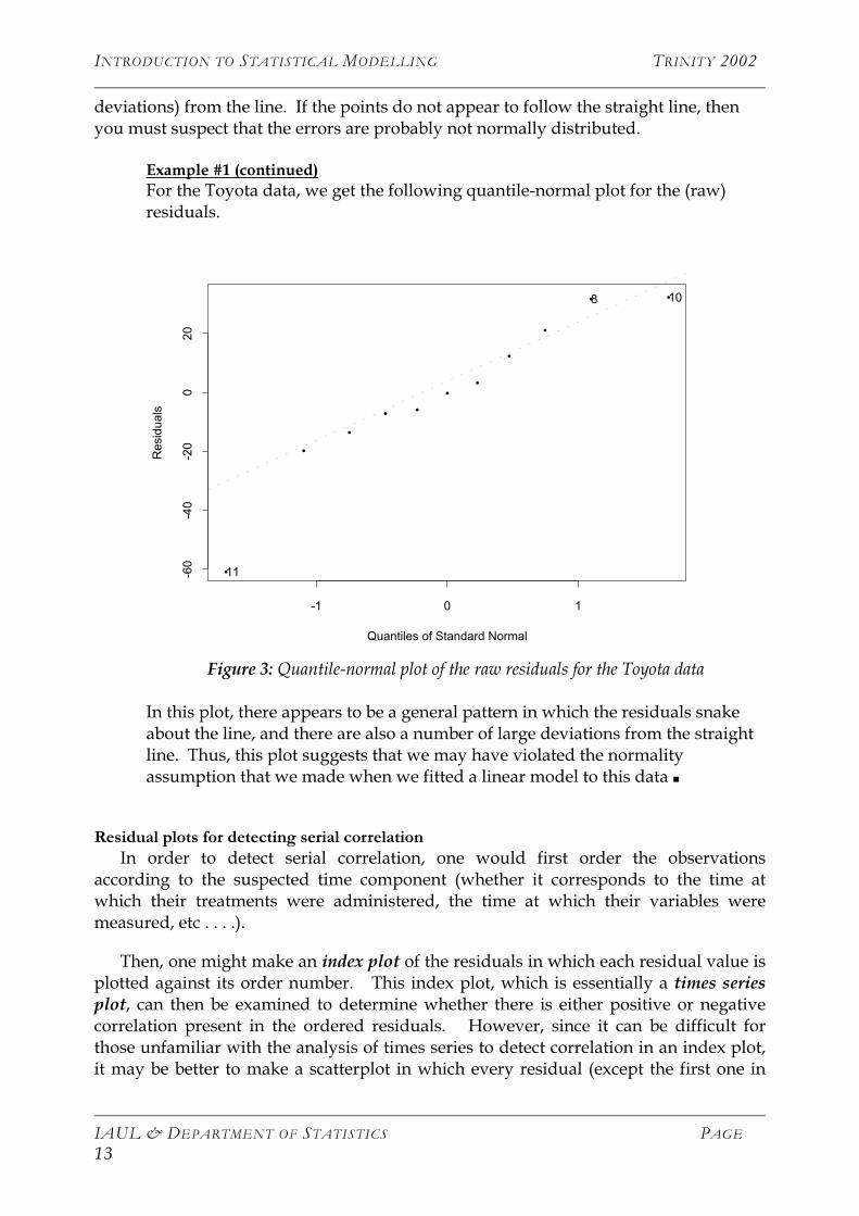
Example #1 (continued) A plot of Cook’s distance for the Toyota data is given below:



Index

Coo

k's

Dis

tanc

e

2 4 6 8 10

0.0

0.5

1.0

1.5

2.0

2.5

8

10

11

Figure 4: Cook’s distances for the 11 observations in the Toyota data example

We note from this plot that observation 11, the one that we have already marked as a residual outlier, appears to have the most weight in the estimation procedure (i.e., it is the most influential). The influence of points 8 and 10 in the above graph mainly comes from the poor quality of the fitted model because of the inclusion of point 11; we should not be concerned that they are linear outliers until we decide how to deal with point 11 ■

If, after a considerable amount of effort, we have succeeded in detecting a linear outlier, what do we do with that observation? This is a very grey area, and different people will argue for different approaches. Two things that people might suggest doing are: 1. Check the quality of the observation(s) that appear to be outliers. This could

involve simply going back to the original data and checking that values have been correctly entered into the computer. However, you might also attempt to actually check the values themselves: it might be possible to go back to the units and re-measure certain variables if they were measured incorrectly at the first attempt. You must be very careful here, though: if the variable that was incorrectly measured is something that can vary over time (e.g., a person’s blood pressure), you have to keep the original measurement. In this approach, if you notice a transcription error or are able to correct a measurement, then you can substitute the correct value into your data set and re-analyse.



2. If the quality of the outlying observation(s) appears to be okay or if it is impossible to check whether they are (as in our example), then you have to proceed very carefully. If you truly believe that the observation is a mistake (i.e., that it would be impossible to observe such a combination of variable values), then you might want to delete the observation from the data and re-analyse without it present. In addition, if you believe the observation to be an anomaly (i.e., it is exceptionally unlikely that you would observe such a combination of values) and you are interested in explaining/predicting the response variable for only those observations that follow the majority linear trend, then you might again consider deleting the observation. Be warned that deletion is a dangerous thing to do: you must be able to give full justification as to why you are deleting observations. Do not fall into the habit of deleting observations simply because doing so makes your model fit much better.

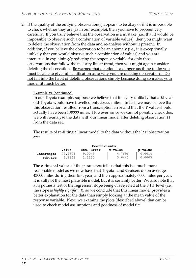
Example #1 (continued) In our Toyota example, suppose we believe that it is very unlikely that a 15 year old Toyota would have travelled only 38000 miles. In fact, we may believe that this observation resulted from a transcription error and that the Y value should actually have been 138000 miles. However, since we cannot possibly check this, we will re-analyse the data with our linear model after deleting observation 11 from the data set. The results of re-fitting a linear model to the data without the last observation are:

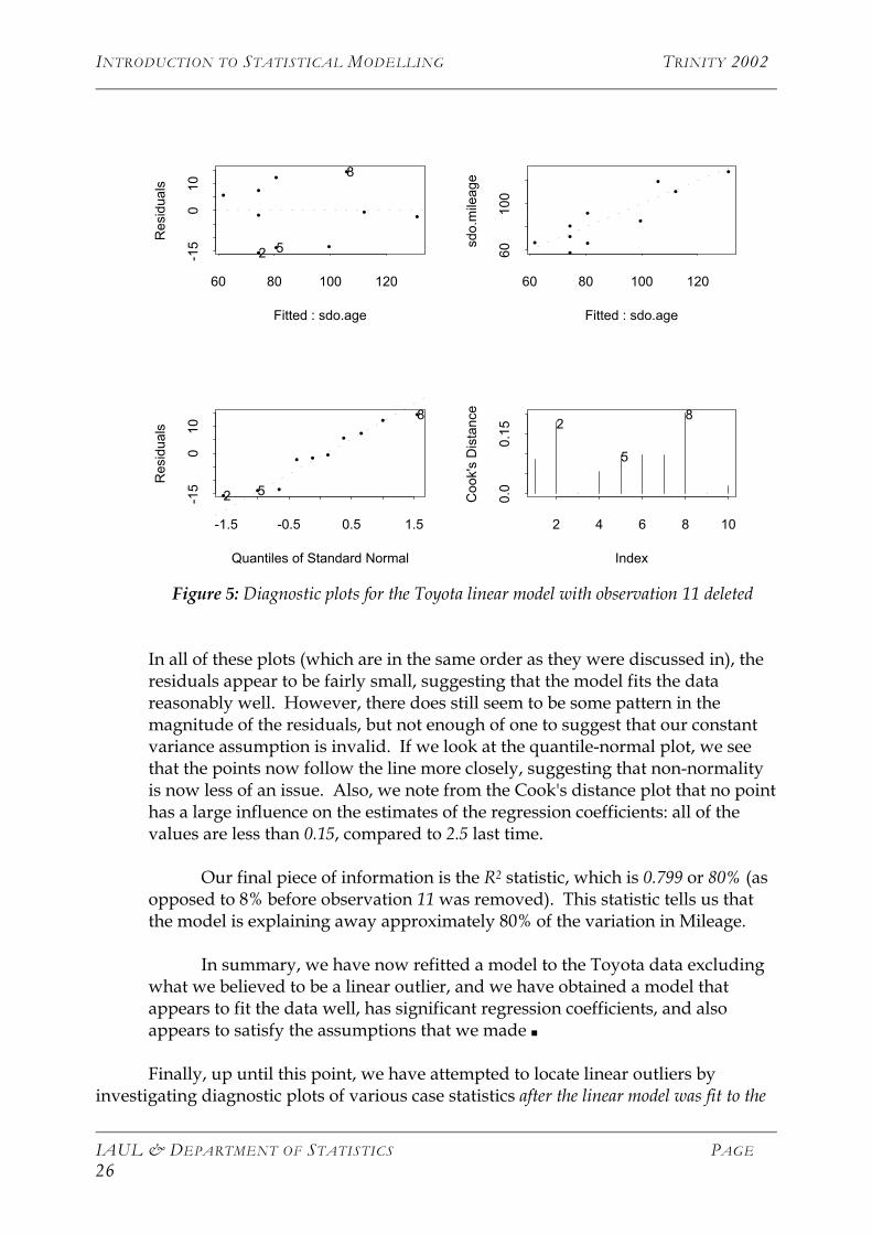
Coefficients Value Std. Error t-value p-value (Intercept) 42.9501 9.0049 4.7696 0.0014 sdo.age 6.2848 1.1135 5.6442 0.0005 The estimated values of the parameters tell us that this is a much more reasonable model as we now have that Toyota Land Cruisers do on average 43000 miles during their first year, and then approximately 6000 miles per year. It is still not the most plausible model, but it is certainly better. We also note that a hypothesis test of the regression slope being 0 is rejected at the 0.1% level (i.e., the slope is highly significant), so we conclude that this linear model provides a better explanation for the data than simply looking at the mean value of the response variable. Next, we examine the plots (described above) that can be used to check model assumptions and goodness of model fit:



•

•

•

•

•

•

•

•

• •

Fitted : sdo.age

Res

idua

ls

60 80 100 120

-15

010

52

8

••••

•

• •

••

•

Fitted : sdo.age

sdo.

mile

age

60 80 100 120

6010

0

•

•

•

•

•

•

•

•

••

Quantiles of Standard Normal

Res

idua

ls

-1.5 -0.5 0.5 1.5

-15

010

52

8

Index

Coo

k's

Dis

tanc

e

2 4 6 8 100.

00.

15

5

28

Figure 5: Diagnostic plots for the Toyota linear model with observation 11 deleted

In all of these plots (which are in the same order as they were discussed in), the residuals appear to be fairly small, suggesting that the model fits the data reasonably well. However, there does still seem to be some pattern in the magnitude of the residuals, but not enough of one to suggest that our constant variance assumption is invalid. If we look at the quantile-normal plot, we see that the points now follow the line more closely, suggesting that non-normality is now less of an issue. Also, we note from the Cook's distance plot that no point has a large influence on the estimates of the regression coefficients: all of the values are less than 0.15, compared to 2.5 last time.

Our final piece of information is the R2 statistic, which is 0.799 or 80% (as opposed to 8% before observation 11 was removed). This statistic tells us that the model is explaining away approximately 80% of the variation in Mileage.

In summary, we have now refitted a model to the Toyota data excluding

what we believed to be a linear outlier, and we have obtained a model that appears to fit the data well, has significant regression coefficients, and also appears to satisfy the assumptions that we made ■

Finally, up until this point, we have attempted to locate linear outliers by investigating diagnostic plots of various case statistics after the linear model was fit to the



data. However, rather than looking for outliers after fitting the model (and then possibly removing them from the data set), you might consider using various fitting techniques, such as least median of squares (LMS) and least trimmed squares (LTS), that are intended to produce estimates of the coefficients that are unaffected by outliers.

A. Roddam (2000), K. Javaras (2002), and W. Vos (2002)


Documents

Stats Lectures - the Department of Statistics