Status on Video Data Reduction and Air Delivery Payload ...faculty.nps.edu/oayakime/ADSC/Scoring - Yakimenko... · Status on Video Data Reduction and Air Delivery Payload Pose Estimation

Status on Video Data Reduction and Air Delivery Payload Pose Estimation

Oleg A. Yakimenko1 Naval Postgraduate School, Monterey, CA 93943-5107

and

Robert M. Berlind2 and Chad B. Albright3 Yuma Proving Ground, Yuma, AZ 85365-9110

The paper discloses a current status of the development and evaluation of an autonomous payload tracking capability for determining time, state and attitude information (TSPI) for all types of airdrop loads. This automated capability of accurately acquiring TSPI data is supposed to radically reduce the labor time and eliminate man-in-the-loop errors. The paper starts with the problem formulation and then reviews the developed software. The algorithms rely on commercial off-the-shelf feature-based video-data processing software adopted for obtaining TSPI. Having the frame coordinates of the centroid of a tracking item available from no less than three ground stationary surveyed cameras at each instant during a descent together with these cameras azimuth and elevation information allows solving the position estimation problem. If more known-geometry features of the airdrop load can reliably be extracted, the pose (position and attitude) estimation would also be possible. The paper primarily addresses the status of the payload’s position estimation portion providing examples of processing video data from up to six cameras. Yet, it also discusses the applicability of more recent computer-vision algorithm, based on establishing and tracking multiple scale-invariant keypoints. The paper ends with conclusions and suggestions for the further development.

I. Introduction Hat

survey

IS paper addresses the problem of determining three-dimensional payload position and possibly payload’s titude based on observations obtained by several fixed cameras on the ground. Figure 1 shows an example of ed camera sites for the combined Corral/Mohave drop zone (DZ), whereas Fig.2 demonstrates an example of

the stabilized Kineto Tracking Mount (KTM) that is used to record the airdrop event from aircraft exit to impact. Figure 2 shows an operator sit (in the center) with multiple cameras (having different focal length). During the drop the operator manually points cameras at the test article. All KTMs have azimuth and elevation encoders which sample Az/El data along with Coordinated Universal Time (UTC) once every video camera frame.

T

There are at least three distinctive reasons for having time, state and attitude information (TSPI) available for each test article. First, it is needed to estimate the performance of the system (e.g., a descent rate at certain altitudes and at touch down). Secondly, this information can be further used for model identification and control algorithms development (see examples in Refs. 1 and 2). Thirdly, parachute- or parafoil-payload systems (including cluster systems) are the multiple-body flexible structures, so knowing the behavior of each component (payload and canopy), as opposed to the center of the whole system, allows to model/improve their interaction.

Obviously, nowadays an inertial measurement unit (IMU) and/or global positioning system (GPS) can be used to acquire accurate TSPI of moving objects. However, when applied to massive testing of different test articles there are several reasons preventing of using those modern navigation means. To start with, you cannot install IMU/GPS 1 Research Associate Professor, Department of Mechanical and Astronautical Engineering, Code MAE/Yk, [email protected], AIAA Associate Fellow. 2 Chief, Air Delivery Systems Branch, Yuma Test Center, [email protected], AIAA Member.

1 American Institute of Aeronautics and Astronautics

3 IT Specialist, Technical Services Division, Yuma Test Center, [email protected], AIAA Member.

19th AIAA Aerodynamic Decelerator Systems Technology Conference and Seminar21 - 24 May 2007, Williamsburg, VA

AIAA 2007-2552

This material is declared a work of the U.S. Government and is not subject to copyright protection in the United States.

units on all test articles (there are to many of them). Second, the harsh condition of operating some of the articles will result in destroying IMU/GPS units each or every other test. Third, some of the test articles simply cannot accommodate IMU/GPS units either because of the size constrains (for instance, bullets and shells) or because of non-rigid structure of the object (canopies). All aforementioned makes using information, recorded by multiple KTMs for each test anyway, to determine TSPI of test articles very relevant.

Figure 1. Two drop zones (stars) with KTM

sites (rhombs). Figure 2. The KTM with the operator seat and multiple

cameras.

KTM / DIVITS VIDEOKTM / DIVITS VIDEO(1(1--10 cameras)10 cameras)

Video Scoring software(VREAD)


ASCII Video File

ASCII Video File

Transfer files to Floppy

Disc


Disc

Transfer files to LINUX


Pre-edit the video files for Time, Azimuth, Elevation and Angle

Errors


Errors

Adjusted ASCII Video

File


File

RAWINRAWIN FileserverFileserver

RAWIN ASCII SFFRAWIN

ASCII SFF

Text Editorfor creating

survey target libraries



ASCII Survey target

File(s)

ASCII Survey target

File(s)

FTP from server to LINUX


Calibrations, Aircraft,Package,

Angles, andOther points of interest



Geodetic Surveyfor camera and

calibration targets


calibration targets

Editing:Verify data

encoding and record

EVENT Times

Editing:Verify data

encoding and record

EVENT Times

TIMES:Establish

common start and stop times per

drop

TIMES:Establish


drop

KTM / DIVITS Calibration(CINCAL)


KTM / DIVITS ODLE Solution

(QDTASK)A/C and PKG


(QDTASK)A/C and PKG

Analyze output:Coordinates,

residuals, position, and

velocities



velocities

Re-runRe-run

Wind and Standard AtmosphereCorrections(NOWIND)PKG data



dynamic pressure,

position, and velocities


dynamic pressure,


Deterministic Attitude

(DETATT):Yaw, pitch, and

oscillation angles



oscillation angles


Yaw, Pitch, and Oscillation

angles



angles

Spline fitting(XPK - XWSFF)Yaw, Pitch, and

Oscillation angles


Oscillation angles

TYPICAL OUTPUTS FOR AIR DROP DATA REDUCTION

A/C Report - Time, Position and Velocity of Aircraft prior and after package release;

PKG Report - Time, Position and Velocity of package (usually center of mass);

Standard Report - Data corrected to Standard day (corrected to standard day density);

Air Drop Report - Test specific output information (impact velocity, etc…);

README - General air drop report file (Drop Zone info, EVENT Times, etc…);

RAWIN - Rawinsonde file corresponding to the closest time of the air drop;

NOWIND - Report file with wind velocities subtracted from the data (optional);

NOWIND/STANDARD - Report of the wind and standard atmosphere corrected data combined (optional).

TYPICAL OUTPUTS FOR AIR DROP DATA REDUCTIONTYPICAL OUTPUTS FOR AIR DROP DATA REDUCTION









Test specific report generation

(ATPS, ECDS, ...)

per customer request


(ATPS, ECDS, ...)


(OPTIONAL)(OPTIONAL)

KTM / DIVITS VIDEOKTM / DIVITS VIDEO(1(1--10 cameras)10 cameras)



ASCII Video File

ASCII Video File


Disc


Disc




Errors


Errors


File


File

RAWINRAWIN FileserverFileserver

RAWIN ASCII SFFRAWIN

ASCII SFF





ASCII Survey target

File(s)

ASCII Survey target

File(s)








calibration targets


calibration targets

Editing:Verify data

encoding and record

EVENT Times

Editing:Verify data

encoding and record

EVENT Times

TIMES:Establish


drop

TIMES:Establish


drop




(QDTASK)A/C and PKG


(QDTASK)A/C and PKG



velocities



velocities

Re-runRe-run




dynamic pressure,



dynamic pressure,




oscillation angles



oscillation angles



angles



angles


Oscillation angles


Oscillation angles

TYPICAL OUTPUTS FOR AIR DROP DATA REDUCTION









TYPICAL OUTPUTS FOR AIR DROP DATA REDUCTIONTYPICAL OUTPUTS FOR AIR DROP DATA REDUCTION










(ATPS, ECDS, ...)



(ATPS, ECDS, ...)


(OPTIONAL)(OPTIONAL)

Figure 3. Current air drop data reduction process.

The current method of video scoring is labor-intensive since no autonomous tracking capability exists.3 This process for capturing/processing the video imagery is summarized in Fig.3. After a drop, during which two to six fixed-zoom ground cameras record the flight, each video is manually “read” for payload position in the field of view. This is accomplished frame by frame, with the video reader clicking on a pixel that represents the visual “centroid” of the payload (from his/her standpoint). Each video frame has a bar code with the azimuth, elevation and

UTC stamp, so the data for each frame is stored automatically as the pixel is clicked. After the videos are read, the data is processed to determine position at each frame during the drop. The payload position is then numerically differentiated to calculate velocity. The automated capability of accurately acquiring TSPI is supposed to hasten the processing of each video by autonomously tracking the payload once initialized. Then data from several cameras can be ‘fused’ together to obtain TSPI (of each object in cameras’ field of view).

Once developed and capable of processing video data off-line, the system can be further transferred into on-line version allowing to exclude KTM operators from manually tracking the payload. After initialization if can be done automatically so that the test article is kept in the center of the frame based on the feedback provided by the estimates/predictions of test article position.

The development of such autonomous capability (TSPI retrieving system) should obviously address the following two independent problems. First, it should process video data itself with the goal of obtaining the frame coordinates of a certain point of the test article, say payload’s geometric center. Second, it should provide the most accurate solution of the position estimation problem assuming that information from two or more cameras situated around DZ is available.

The appropriate software to solve each of two problems has been developed and successfully tested in simulations and with the use of real drop data, so in what follows Sections II and III address each of these problems.

II. Video Data Processing The goal of the video data processing is to prepare all necessary data for the following test item position

estimation. For offline position estimation it is possible to either use a live recorded video stream or to break it onto sequences of bmp-files and to work with them instead. The software developed to support video data processing consists of several executable files as well as multiple MATLAB M-files having a user-friendly interface. To make the software more flexible (allowing dealing with different portions of algorithms separately) the video data processing was broken into four stages.4

Stage 1 deploys the PerceptiVU Snapper, developed by PerceptiVU, Inc. (www.PerceptiVU.com) to break the live digital video coming out of the video player onto the sequence of bmp-files (Fig.4 demonstrates the first and the last files of sample sequence). The output of this stage is the sequence of bmp-files to work with during the following stages.

Figure 4. The first and the last slices of the video.

Stage 2 reads the bar code from bmp-files obtained at the previous stage and renames these bmp-files to allow further batch processing. The outputs from this stage are the sequence of renamed (having uniform name) bmp-files and ASCII file containing bar-code data.

Stage 3 uses another piece of software developed by PerceptiVU, Inc., namely PerceptiVU Offline Tracker to retrieve x-/y-offsets of the center of the test item from each image (renamed bmp-file). The PerceptiVU Tracker window with several drop-down option windows is shown on Fig.5. For the batch processing a user encloses the test article to track into the appropriate-size box on the very first frame and then starts tracking. The output of this stage is the ASCII file containing x-/y-offsets.

Once the previous stages are completed on the video streams pertaining to all cameras involved in the specific drop, Stage 4 takes care of data conditioning, correction and synchronization. All Az/El files and x-/y-offsets files obtained at the previous stage for multiple cameras are being processed automatically. While checking and correcting all the data the MATLAB script displays all relevant results.

http://www.perceptivu.com/

First, it checks the time stamp in the Az/El data and displays the results for all cameras as shown on Fig.6. Upper plots display UTC time as retrieved from the bar-code versus bmp-file number. All dropouts or frames corresponding to any suspicious (non-monotonic) behavior are marked with the red vertical bars. The bottom plots show a frame rate. In case of any abnormalities with the time stamp (on the upper plots), its value is restored using an average frame rate (shown as a horizontal dashed red line on the bottom plots).

Second, the loaded x-/y-offsets for each camera are analyzed and displayed in several ways. The power spectrum for x- and y- offsets shows up as presented on Fig.7a. The yellow trace around it indicates the quality of data (standard deviation). If it is too wide, there might be some problems with the data. Another way to visually check the quality of the data is to look at the second type of plots showing up for each camera (Fig.7b). Here the user can observe the Welch power spectrum density (PSD) for both offsets as well as strip offsets themselves.

Figure 5. Setting the options for the PerceptiVU Tracker.

Figure 6. Correcting UTC stamps using the average fragmentation rate.

Third, the UTC stamp is being added to the x-/y-offset data. It is taken from the Az/El data files corresponding to the same camera. The x-/y-offsets files are synchronized with the corresponding Az/El files starting from the last frame and moving backward. Once the time stamp to x-/y-offsets files is added, the script continues with checking/correcting (eliminating corrupted lines) the data in these files. After fixing it, the program proceeds with checking the consistency of the data. It’s being done for both offsets for each camera as shown on Fig.8. The 128-point Welch window runs through the centered offsets data. If the Welch PSD approaches or drops below 10-5 (marked with the wide green strip in the bottom portion of the bottom plots), it indicates that something is wrong with the data and those suspicious points should be eliminated (the wide strip itself turns yellow or red, respectively).

Similarly the x-/y-offset data is also checked for the spikes and dropouts and corrected as presented on Fig.9.

a) b) Figure 7. Power spectrum (a) and Welch PSD estimates for x- and y- offsets for each camera.

Figure 8. Checking/correcting time histories of the x- and y- offsets.

Figure 9. Checking/correcting dropouts and spikes in azimuth/elevation data.

When all data for each specific camera has been processed, the complete information from all cameras is analyzed all together to establish the common time range. The data that falls beyond this range is eliminated.

Eventually, four aforementioned stages produce the ASCII files containing conditioned and synchronized Az/El and x-/y-offsets files for all cameras ready to be passed to the position estimation algorithm. An example of such data for three cameras is shown on Fig.10. The top plots represent Az/El data form the release point down to impact point, whereas the plots beneath them demonstrate a position of payload’s centroid within each camera’s frame. As seen, KTM operators do a very good job keeping the test article in the center of the frame.

III. Payload Position Estimation

This section discusses algorithm that finds the three-dimensional position ( ) ( ), ( ), ( )T

pl pl plt x t y t z t⎡ ⎤= ⎣ ⎦P of the

payload’s centroid, when its projection { ( , i=1,…,N onto the image plane of N cameras is available. It is

assumed that the position

), ( )}i ipl plu t v t

, ,Ti i i i

c c cx y z⎡= ⎣C ⎤⎦ ) of each camera in the local tangent plane (LTP or {u}), as well as their

focal length, fi, azimuth, ( )iAz t , and elevation, , are known. ( )iEl t

Figure 10. Example of synchronized data for three cameras.

In the absence of measurement errors the following equalities hold for each instance of time:

1

100

cos tan

i

ipliii

uAz

f−

⎡ ⎤⎢ ⎥⎡ ⎤−⎣ ⎦ ⎢ ⎥

⎛ ⎞⎢ ⎥⎣ ⎦ = +⎜ ⎟⎜ ⎟⎡ ⎤− ⎝ ⎠⎣ ⎦

R C P

R C P, 1

001

cos tan

Ti

ipliii

vEl

f−

⎡ ⎤⎢ ⎥⎡ ⎤−⎣ ⎦ ⎢ ⎥

⎛ ⎞⎢ ⎥⎣ ⎦ = +⎜⎜− ⎝ ⎠

C P

C P⎟⎟ (1)

(here ). ([1,1,0])diag=RHowever, since the measurement errors are always present these two equalities become inequalities and can be

rewritten using residuals iEl∆ and as i

Az∆

1

001

cos tan

Ti

ipli i

Elii

vEl

f−

⎡ ⎤⎢ ⎥⎡ ⎤−⎣ ⎦ ⎢ ⎥

⎛ ⎞⎢ ⎥⎣ ⎦ − + =⎜ ⎟⎜ ⎟− ⎝ ⎠

C P

C P∆ and 1

100

cos tan

i

ipli i

Azii

Ru

AzfR

−

⎡ ⎤⎢ ⎥ ⎡ ⎤−⎣ ⎦⎢ ⎥

⎛ ⎞⎢ ⎥⎣ ⎦ − + =⎜ ⎟⎜ ⎟⎡ ⎤− ⎝ ⎠⎣ ⎦

C P

C P∆

)

. (2)

Therefore, each camera contributes two nonlinear equations of the form (2). That is where it follows from that to resolve the original problem for three components of the vector P we need to have at least two cameras (N≥2).

Whereas a lot of algorithms to address the pose estimation problem (determining components of the vector ) exists (e.g., see references in Ref. 4), we cast this problem as the multivariable optimization problem. Having full information from N≥2 cameras it is needed to find the vector that minimizes the compound functional:

P

P

( 2 2

1

Ni iAz El

iJ

=

= ∆ + ∆∑ . (3)

This problem is solved using a Simulink model that employs a standard MATLAB fminsearch function for unconstrained non-linear minimization (based on the non-gradient Nelder-Mead simplex method5). The developed routine proved to be reliable and quite robust in handling both emulated and real drop data.

Figure 11 shows the results of processing the data of Fig10. It also shows the results of the descent rate estimate. For this particular drop the GPS/IMU data was also available. So comparison with this data demonstrated a perfect match (with an average error of less than 2m that corresponds to the cameras’ pixel size).

To validate developed algorithms in the field conditions, data from a personnel airdrop at Sidewinder DZ was collected from six cameras. The output plots for the personnel airdrop are shown in Fig.12. This figure shows an excellent performance of the algorithms with a smooth position output (top two plots), and nominal x-y-z coordinate display estimate (the lower left plot). The vertical velocity (time-differentiated z-position) plot in the lower right corner is typical of this type of systems, with higher frequency peaks due to jumper oscillation and small changes of the tracker lock in the vertical direction. A simple one-dimensional digital MATLAB filter function was used with a window size of 80 samples to display the running average of the descent rate as shown by the trace. A specification limit is depicted with the horizontal line for visual assessment.

Figure 11. Position and descent rate estimation using data of Fig.10.

Figure 12. Estimation of the position and descent rate for the personnel airdrop.

Figures 13 and 14 demonstrate the results for one more cargo drop (also at Sidewinder DZ), which also employed six cameras. The top-left plot on Fig.13 presents the bird’s eye view of the KTM constellation around the release point (radial lines show the direction to the test article at the release (solid lines) and impact points (dashed lines)). The bottom plot depicts the Az/El data for all six cameras. The top-right plot demonstrates the estimate of

the geometric dilution of precision (GDOP), i.e. the maximum accuracy that can be possibly achieved (primarily based on the cameras’ pixel resolution). Figure 14 shows the result of processing this six-camera data.

Figure 13. Results of the video data processing for the six-camera cargo drop.

Figure 14. Position and descent rate estimation for the cargo airdrop presented on Fig.13.

IV. Graphical User Interface To support further development, the user-friendly graphical user interface (GUI) was developed (Fig.15). This

two-page GUI allows visualizing the real drop data, as well as analyzing emulated trajectories with the goal of assessing a visibility of enough geometry-based features (for pose estimation). Based on the YPG DZ/KTM data base the first page lets a user to choose any specific drop zone from the pop-up menu and the KTM constellation used in the specific drop (Fig.15a). Then, the user navigates to the directory containing the real-drop / emulated data. Next, he/she proceeds to the second page (Fig.15b), where a 3D trajectory along with the simulated images from all (up to six) involved cameras is animated. The user can change the view point for the 3D trajectory (by moving azimuth and elevation sliders), “experiment” with the focal length of each camera, and “freeze” simulation at any instant of time.

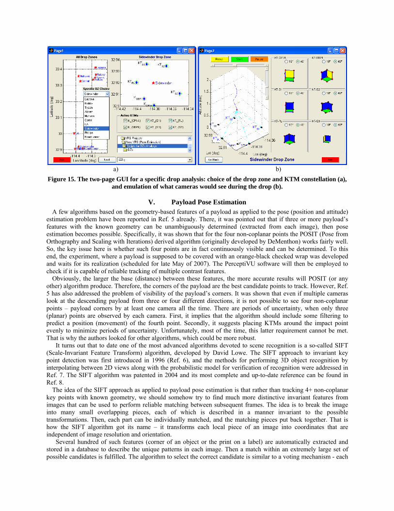
a) b)

Figure 15. The two-page GUI for a specific drop analysis: choice of the drop zone and KTM constellation (a), and emulation of what cameras would see during the drop (b).

V. Payload Pose Estimation A few algorithms based on the geometry-based features of a payload as applied to the pose (position and attitude)

estimation problem have been reported in Ref. 5 already. There, it was pointed out that if three or more payload’s features with the known geometry can be unambiguously determined (extracted from each image), then pose estimation becomes possible. Specifically, it was shown that for the four non-coplanar points the POSIT (Pose from Orthography and Scaling with Iterations) derived algorithm (originally developed by DeMenthon) works fairly well. So, the key issue here is whether such four points are in fact continuously visible and can be determined. To this end, the experiment, where a payload is supposed to be covered with an orange-black checked wrap was developed and waits for its realization (scheduled for late May of 2007). The PerceptiVU software will then be employed to check if it is capable of reliable tracking of multiple contrast features.

Obviously, the larger the base (distance) between these features, the more accurate results will POSIT (or any other) algorithm produce. Therefore, the corners of the payload are the best candidate points to track. However, Ref. 5 has also addressed the problem of visibility of the payload’s corners. It was shown that even if multiple cameras look at the descending payload from three or four different directions, it is not possible to see four non-coplanar points – payload corners by at least one camera all the time. There are periods of uncertainty, when only three (planar) points are observed by each camera. First, it implies that the algorithm should include some filtering to predict a position (movement) of the fourth point. Secondly, it suggests placing KTMs around the impact point evenly to minimize periods of uncertainty. Unfortunately, most of the time, this latter requirement cannot be met. That is why the authors looked for other algorithms, which could be more robust.

It turns out that to date one of the most advanced algorithms devoted to scene recognition is a so-called SIFT (Scale-Invariant Feature Transform) algorithm, developed by David Lowe. The SIFT approach to invariant key point detection was first introduced in 1996 (Ref. 6), and the methods for performing 3D object recognition by interpolating between 2D views along with the probabilistic model for verification of recognition were addressed in Ref. 7. The SIFT algorithm was patented in 2004 and its most complete and up-to-date reference can be found in Ref. 8.

The idea of the SIFT approach as applied to payload pose estimation is that rather than tracking 4+ non-coplanar key points with known geometry, we should somehow try to find much more distinctive invariant features from images that can be used to perform reliable matching between subsequent frames. The idea is to break the image into many small overlapping pieces, each of which is described in a manner invariant to the possible transformations. Then, each part can be individually matched, and the matching pieces put back together. That is how the SIFT algorithm got its name – it transforms each local piece of an image into coordinates that are independent of image resolution and orientation.

Several hundred of such features (corner of an object or the print on a label) are automatically extracted and stored in a database to describe the unique patterns in each image. Then a match within an extremely large set of possible candidates is fulfilled. The algorithm to select the correct candidate is similar to a voting mechanism - each

feature votes for the candidate, which includes a similar feature (e.g., a corner feature in the new image that matches a corner feature in a trained image). The correct candidate receives the largest number of votes since most of the features are in agreement. However, a single or a few votes might be incorrectly cast on wrong candidates. The likelihood that a large number of votes are cast on the wrong candidate is supposedly to be small, demonstrating that the algorithm should be very reliable in selecting the correct match.

Figure 16b show an example of such features found by SIFT for the very same image we were looking at earlier, when establishing four non-coplanar points to track (Fig.16a). For this particular image there are 137 automatically defined points versus only four, assigned manually. Suppose one fourth of the found features will not find their matches on the subsequent frame –we will still have about a hundred other matches. Compare it to what would happen when a single point in a four-point scheme is missing or found incorrectly.

Figure 16. One of the real drop images featuring 137 scale-invariant key points (b) as opposed to just four,

assigned artificially (a).

Supposedly, local invariant features allow us to efficiently match small portions of cluttered images under arbitrary rotations, scalings, change of brightness and contrast, and other transformations. Evolution Robotics ViPR™ (visual pattern recognition) technology (www.evolution.com) incorporates SIFT already and provides a reliable and robust vision solution that truly gives different electronic devices the ability to detect and recognize complex visual patterns. As claimed by the Evolution Robotics, ViPR software assures the following performance/features:

• 80-100% recognition rate depending on the character of the objects to recognize; • works for a wide range of viewing angles, lens distortion, imager noise, and lighting conditions; • works even when a large section (up to 90%) of the pattern is occluded from the view by another object; • can simultaneously recognize multiple objects; • can handle databases with thousands of visual patterns without a significant increase in computational

requirements (the computation scales logarithmically with the number of patterns); • can process 208x160 pixel images at approximately 14-18 frames per second using a 1400 MHz PC; • can automatically detect and recognize visual patterns using low- or high-end camera sensors (with heavy

distortions that can be introduced by the imaging device, a wide range of lighting conditions, and pattern occlusions).

However, as the following analysis revealed, the SIFT algorithm only works fine in a specific environment. Figure 17 demonstrates that the hope that among those over-a-hundred features found on each image (Fig.16b) the majority will find their match on the subsequent images did not prove true. To this end, Fig.17a compares Frame 1 vs. Frame 2 (taken within 1/30=0.03sec). It shows only 21 matching key points. The comparison of Frame 1 and Frame 3 (2/30=0.07sec apart) reveals as little as 10 matching key points (Fig.17b). Frame 1 vs. Frame 4 (3/30=0.1sec) yields 5 matching key points (Fig.17c), and Frame 1 vs. Frame 8 (7/30=0.23sec) – a single matching key point (Fig.17d). In just eight frames (about a quarter of a second apart) there is no match at all! Moreover, the matching points found on the further-apart images are not necessarily show up on the closer-apart images, i.e. there is no consistency.

Although the key points are claimed to be invariant to scale and rotation, so that they should provide robust matching across a substantial range of affine distortion, change in 3D point, noise, and change in illumination, the SIFT algorithm failed to demonstrate it. The main reason for the failure is that the payload in the image occupies only about 50x30 pixels. On top of that, there are huge compression artifacts. Hence, it is believed that if the camera resolution is increased and/or the amount of lossy compression is reduced, then the algorithm might work better. It

http://www.evolution.com/

would also help if the payload itself had some kind of printed pattern on it to provide more reliable SIFT features than the ones currently used. This brings us back to the idea of having payload wrapped with a contrast cover with some pattern.

a) b)

c) d)

Figure 17. The key features matches on the subsequent images: frames 1 and 2 (a), 1 and 3 (b), 1 and 4 (c), 1 and 8 (d).

VI. Conclusion All components of the combined video-data-retrieving and position estimation algorithm have been developed

and tested. Autonomous video scoring of air delivery payloads significantly improves the current method of extracting TSPI from video imagery manually. Although the manpower reduction was not quantified, the labor benefit from autonomous scoring is obvious. Without the man-in-the-loop, the potential for errors is also reduced. Being inspired by the results of estimating time histories of test articles’ position and speed, the authors continue their efforts to be also able to estimate an angular position (attitude) of the tracked test item. The four-geometry-based-non-coplanar-point algorithm reported earlier was perfected to the point, where additional tests are needed to verify the core concept. The standalone GUI was also developed to support further research. In parallel, another, not geometry-based, but rather scale-invariant-keypoints approach was tested but failed to demonstrate acceptable performance. The authors rely on the upcoming tests to try to improve this latter approach robustness via artificially adding more features to a payload.

References 1 Dobrokhodov, V.N., Yakimenko, O.A, and Junge, C.J., “Six-Degree-of-Freedom Model of a Controlled Circular

Parachute”, AIAA Journal of Aircraft, Vol.40, No.3, 2003, pp.482-493. 2 Yakimenko, O., and Statnikov, R., “Multicriteria Parametrical Identification of the Parafoil-Load Delivery

System,” Proceedings of the 18th AIAA Aerodynamic Decelerator Systems Technology Conference, Munich, Germany, 24-26 May 2005.

3 Albright, C., et al., “Processing of Time Space Position Information Data,” Process documentation, continually updated, Yuma Proving Ground, AZ, 1995-present.

4 Yakimenko, O.A., Dobrokhodov, V., Kaminer, I., and Berlind, R., “Autonomous Video Scoring and Dynamic Attitude Measurement,” Proceedings of the 18th AIAA Aerodynamic Decelerator Systems Technology Conference, Munich, Germany, 24-26 May 2005.

5 Lagarias, J.C., Reeds, J.A., Wright M.H., and Wright, P.E., “Convergence Properties of the Nelder-Mead Simplex Method in Low Dimensions,” SIAM Journal of Optimization, Vol.9, No.1, 1998, p.112-147.

6 Lowe, D.G., “Object Recognition from Local Scale-Invariant Features,” International Conference on Computer Vision, Corfu, Greece, September, 1999, pp.1150-1157.

7 Lowe, D.G., “Local Feature View Clustering for 3D Object Recognition,” IEEE Conference on Computer Vision and Pattern Recognition, Kauai, Hawaii, December 2001, pp.682-688.

8 Lowe, D.G., “Distinctive Image Features from Scale-Invariant Keypoints,” International Journal of Computer Vision, Vol.60, No.2, 2004, pp.91-110.

Documents

Status on Video Data Reduction and Air Delivery Payload ...faculty.nps.edu/oayakime/ADSC/Scoring - Yakimenko... · Status on Video Data Reduction and Air Delivery Payload Pose Estimation