Energy Conuers. Mgmt Vol. 38 No. 8, pp. 787-798, 1997 0 1997 Elsevier Science Ltd Pergamon

Pll:so196-89oq%)ooo864 Printed in GreaiBritain. AU rights reserved

0196-8904/97 $17.00 + 0.00

OPTIMIZATION OF SOLAR POND ELECTRICAL POWER GENERATION SYSTEM

R. A. HAJ KHALIL,’ B. A. JUBRAN’t and N. M. FAQIR’ Department of Mechanical Engineering, 2Department of Chemical

Amman, Jordan

(Received 21 September 1995)

Engineering, University of Jordan,

Abstract-This paper investigates the potential of using a solar pond for the generation of electricity in Jordan. A solar pond power plant model is presented to simulate and optimize such a system under the Jordanian climatic conditions. A Rankine cycle analysis is carried out using an environmentally friendly working fluid, Refrigerant 134a.

It was found that using a solar pond for the generation of electricity in Jordan has the potential, with the cost of 0.234 JDjkWh when using a pond of surface area of 1.5 km’, to generate 5 MWe. 0 1997 Elsevier Science Ltd. All rights reserved.

NOMENCLATURE A = Surface area of pond

Ab = Bottom area of pond AF = Area factor

C,, Cr = Empirical constants C, = Water specific heat dg = Distance betweeen solar pond bottom and heat sink in ground

frac(x)ncz = Fraction of solar radiation remaining at depth x H = Daily total solar radiation at horizontal surface

H, = Average of H hr = Number of hours in day

I = Hourly total solar radiation at horizontal surface i = Interest rate

k, = Brine thermal conductivity kr = Ground thermal conductivity e, = Thickness of LCZ /. = Thickness of UCZ L, = Heat extraction depth Cr = Distance of heat sink for bottom of pond m = Mass of brine at storage zone n = Number of days P = Pond perimeter x = Pond total depth

,xNCz = Nonconvective zone depth Q bO,fDm = Bottom and side heat losses

Qp,. = Energy gain by solar radiation Q,= = Total heat losses from storage zone Qtop = Top heat losses Qsh = Greenhouse load

y1 = Ratio of hourly total radiation to daily total radiation T. = Storage zone temperature r, = Ground heat sink temperature

T., = Ambient temperature T,,. = Minimum temperature T,. = Maximum temperature

t = Time 1, = Solar time

U,, = Bottom loss coefficient U,, = Top loss coefficient e, B = Empirical constant

TAuthor to whom correspondence should be addressed.

787

188 HAJ KHALIL er al.: SOLAR POND ELECTRICAL POWER

p = Brine density 6 = Declination angle 4 = Latitude angle for solar pond location o = Hour angle wI = Sunset angle r = Greenhouse cover transmittance

1. INTRODUCTION

Solar ponds are characterized by their ability to collect large amounts of solar radiation and, at the same time, provide long term energy storage. Solar ponds may be used as a heat source for many applications, one of which is the generation of electricity. Bronicki [l] pointed out some of the attractive merits for solar pond power generation plants, such as no fossil fuel is necessary, low running cost, use of local resources, and they do not pollute the environment.

Numerical modelling of solar ponds has been reported by many investigators to predict the temperature and salinity profiles in the pond, as well as the prediction of the stability of the solar ponds. A good account of this is given in a recent paper by Bardran et al. [2]. Most of these investigations make use of a one dimensional model and use either finite elements or finite difference methods to solve such models [3-51. Xe et al. [6] reported a methodology for the prediction of internal stability in solar ponds.

Most works conducted on solar pond electrical power generation systems are associated with the analysis of the system on a certain cycle and working fluid. The most common cycle used is the Rankine cycle-base heat engine operating between the high and low temperatures of the pond [7]. Bechtel[8] investigated a solar pond power plant using F-l 1 as the working fluid when the pond is 1 km2. It was concluded that the cost of the solar pond power plant is five times larger than that of a conventional power plant of equal capacity. Many studies were also reported in the literature about dual purpose plants [9] where they used the plants for electricity generation and water desalination. Numerous works on solar pond electrical power generation have been reported in Moshref [lo].

To the best of the authors’ knowledge, it appears that there is no study in the open literature regarding solar pond power plant generation under the Jordanian climate, as well as using an environment-friendly working fluid, such as Refrigerant 134a (1,l ,I ,2_tetrafluoroethane).

2. MATHEMATICAL MODEL

A one dimensional model for the solar pond has been used to predict the temperatures in the storage zone. The model is similar to that used by Al-Qassem [l 11. The power cycle analysis and the optimization procedure used are that of Moshref [lo].

A one dimensional model is used to predict the solar pond characteristics. This model assumes the storage zone to be fully mixed with the effect of convective layers generated by the side walls being negligible. Furthermore, the boundaries motion of both the upper convective and the lower convective zones have been neglected.

The energy balance equation for the lower convective zone may be written as

dTs mcp dt = Qgain - Qm - &ad (1)

where c,, m and T, are the specific heat, the mass of saline water and the temperature in the storage zone, respectively. Using finite differences, equation (1) may be written as

T,' = T, + e (Qgain - Q~oss - Qload). (2) P

The heat gain from the solar radiaton is obtained from

Qpin = frac(x)NcZ x I x A (3)

HAJ KHALIL ef al.: SOLAR POND ELECTRICAL POWER 789

where frac(x& is the fraction of solar radiation reaching depth x which is defined by one of the following equations [12, 131:

frac(x) = 0.36 - 0.08 In(x)

frac(x) = 0.3 13 exp( -0.28x). (4)

The hourly solar radiation that reaches the horizontal surface of the pond is I, which is related to the monthly average value by [14]

I=y,xz7 (5)

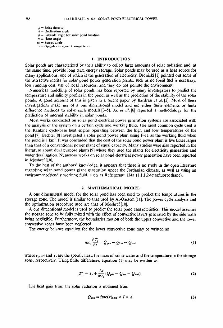
Fig. I. Flow chart for the computational program procedure.

790 HAJ KHALIL et al.: SOLAR POND ELECTRICAL POWER

Table 1. Summary of the cost of the system components

No.

1

System components

Pond Liner Waver damper Excavation Pre-heater area Boiler area Condenser area Pumps Turbine Generator

cost -

6 JD/m* 24 JD/m2 36 JD/m’

240 JD/m’ 240 JD/m’ 240 JD/m’

480 JD/kW 600 JDjkW 600 JDikW

where yr is the ratio of the hourly total to daily total radiation and it is given by

g,=$(a+bcoso) cos w - cos OS

2no * sin oS - 360 ( ) cos 0,

(6)

The coefficients a and b are given by

a = 0.409 + 0.502 sin(w, - 60) b = 0.661 + 0.477 sin(o, - 60) (7)

where oS is the sunset hour angle in degrees and is found from

0, = cos-‘( - tan 4 tan 6) (8)

where 4 is the latitude angle for the pond location and 6 is the declination angle. The hour angle o or the angular displacement of the sun east or west of the local meridian due to rotation of the earth on its axis at 15” per hour is given by

0 = lS(t, - 12). (9)

The total heat loss from the storage zone consists of two parts; one part is due to heat losses through the non-convective zone caused by the temperature difference between the storage and the ambient, and the other part is the losses from the solar pond wall and bottom, i.e.

Q~oss = Qtop + Qbottom. (10)

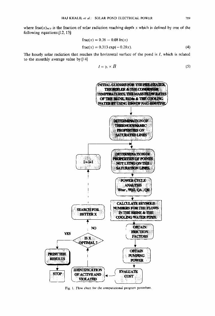
QUAKER (1991-1993)

Fig. 2. Solar radiation variation in Jordan during the period of 1991-1993.

HAJ KHALIL et al.: SOLAR POND ELECTRICAL POWER

Table 2. Summary of results of SPPP for A = 0.75 km2

791

Item Description

Solar ponds

Turbine

Surface area Heat extraction depth Temperature of LCZ Pond efficiency

Inlet temperature Inlet pressure

0.75 km2 1.5 m 79°C 14.2%

70°C 2.12 MPa

Condenser Inlet temperature Inlet nressure

26°C 0.686 MPa

Net electrical power 5.3 MW

The top heat loss is given by

Qtop = Um,(Ts - Tan+ (11)

where UtoP is the top loss heat transfer coefficient, kl/xNCZ, with k, being the brine thermal conductivity. The ambient temperature is assumed to be a sinusoidal function given by

Tamb = Tmm - (T,,, - T,,,,)cos fi x (hr) - : . (12)

Hull et al. [ 151 have developed the following empirical equation to calculate the bottom and side losses:

where Ab and P are the bottom area, and the bottom constants are expressed as

B = CA(Ts - T,).

(13)

perimeter, respectively. The empirical

(14)

(15)

The constants C, and C2 are 0.99 and 0.9 [16]. Equation (13) may be written in terms of equations (14) and (15) as

u botram = U,,(Ts - T&k (16)

G 70

C 60

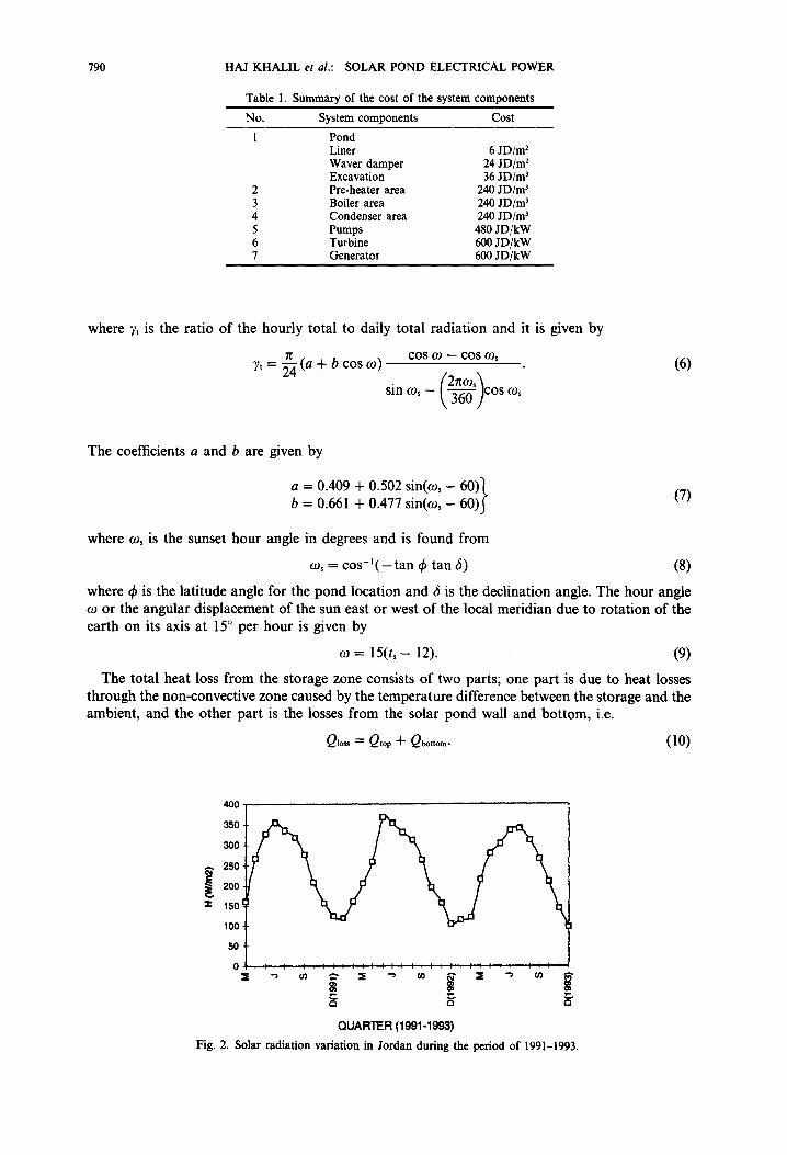
T&=3 T(twbine) T(condensw)

Fig. 3. Variations of the optimum LCZ, the turbine and condenser temperatures for Jordan when A = 0.75 km*.

792 HAJ KHALIL et al.: SOLAR POND ELECTRICAL POWER

where

&Of = Cl@ + Gk*(-g (17)

The static efficiency of a solar pond is the ratio of the average heat extracted to the average value of the solar radiation incident upon the pond surface as follows [lo]:

where % is the average of H, and 0 is given by

and F is a factor given by

(19)

where qn and pLn are weighting and absorption coefficients, respectively, where values for these are given by Rable and Nielsen [17] and Crevier [ 181. The coefficient pn* is given as

pn* = pLn set Bz (21)

where 8, is dependent on the refractive index of the air nl, the refractive index of the pond n2 and the incidence angle f3,, which is given by

t% = arcsin z sin 0, [ 1 . (22)

The working fluid used in the present work is R134a and the cycle analysis is found in Ref. [lo], and only the optimization problem will be outlined in this paper.

The cost of a solar pond power plant (SPPP) is given by a nonlinear function that is to be minimized. The total installation cost consists of the solar pond (Cpd), land (C,), pumps (C,,,,), boiler (C,), condenser (CJ, preheater (Cph), generator (C,), and turbine (Cl) costs. The total cost, Ct is given by

(23)

March

13 13.5 14 14.5 15

Pond efficiency (%)

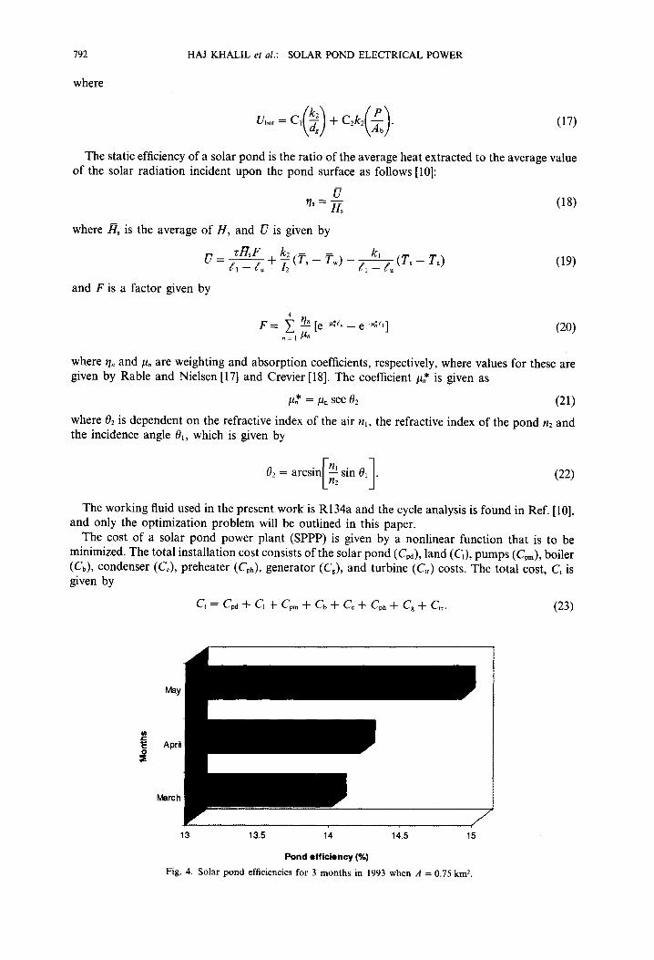
Fig. 4. Solar pond efficiencies for 3 months in 1993 when A = 0.75 km*.

HAJ KHALIL et al.: SOLAR POND ELECTRICAL POWER 793

electrical power

April

Months

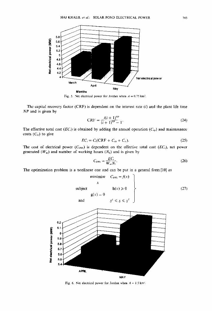
Fig. 5. Net electrical power for Jordan when A = 0.75 km’.

The capital recovery factor (CRF) is dependent on the interest rate (i) and the plant life time NP and is given by

The effective total cost (EC,) is obtained by adding the annual operation (C,,) and maintenance costs (Cm) to give

EC, = C,(CRF + Cop + C,). (25) The cost of electrical power (C,,,) is dependent on the effective total cost (EC,), net power generated (W.J and number of working hours (N,,) and is given by

The optimization problem is

C EC, -- kWh - WnrNh’

a nonlinear one and can be put in a general form [lo] as

minimize CkWh =f(x)

X

subject h(x) > 0

g(x) = 0 and .+ 6 ;u < .x1’ :

(27)

Fig. 6. Net electrical power for Jordan when A = 1.5 km’.

794 HAJ KHALIL et al.: SOLAR POND ELECTRICAL POWER

??Pond efficiency (%)

14.5 15 15.5 16 16.5 17 17.5 16

Efficiency (%)

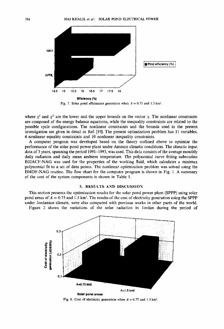
Fig. 7. Solar pond efficiencies generation when A = 0.75 and 1.5 km*.

where xL and $’ are the lower and the upper bounds on the vector x. The nonlinear constraints are composed of the energy balance equations, while the inequality constraints are related to the possible cycle configurations. The nonlinear constraints and the bounds used in the present investigation are given in detail in Ref. [19]. The present optimization problem has 11 variables, 4 nonlinear equality constraints and 10 nonlinear inequality constraints.

A computer program was developed based on the theory outlined above to optimize the performance of the solar pond power plant under Amman climatic conditions. The climatic input data of 3 years, spanning the period 1991-1993, was used. This data consists of the average monthly daily radiation and daily mean ambient temperature. The polynomial curve fitting subroutine E02ACF-NAG was used for the properties of the working fluid, which calculates a minimax polynomial fit to a set of data points. The nonlinear optimization problem was solved using the E04DF-NAG routine. The flow chart for the computer program is shown in Fig. 1. A summary of the cost of the system components is shown in Table 1.

3. RESULTS AND DISCUSSION

This section presents the optimization results for the solar pond power plant (SPPP) using solar pond areas of A = 0.75 and 1.5 km*. The results of the cost of electricity generation using the SPPP under Jordanian climate, were also compared with previous works in other parts of the world.

Figure 2 shows the variations of the solar radiation in Jordan during the period of

0.3

0.2

0.1

Solar pond areas A=1.5 kriQ T

Fig. 8. Cost of electricity generation when A = 0.75 and 1.5 km*.

HAJ KHALIL ef al.: SOLAR POND ELECTRICAL POWER 795

Steam(ACHussien)

Gas turbines/Diesel

Dieselengines

0 0.05 0.1 0.15 0.2 0.25

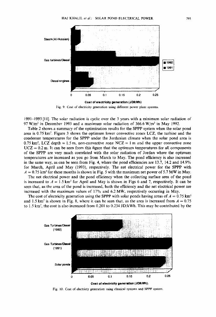
Cost of electricity generation (JMtwh) Fig. 9. Cost of electricity generation using different power plant systems.

1991-1993 [ll]. The solar radiation is cyclic over the 3 years with a minimum solar radiation of 97 W/m2 in December 1993 and a maximum solar radiation of 366.6 W/m* in May 1992.

Table 2 shows a summary of the optimization results for the SPPP system when the solar pond area is 0.75 km2. Figure 3 shows the optimum lower convective zones LCZ, the turbine and the condenser temperatures for the SPPP under the Jordanian climate when the solar pond area is 0.75 km*, LCZ depth = 1.5 m, non-convective zone NCZ = 1 m and the upper convective zone UCZ = 0.2 m. It can be seen from this figure that the optimum temperatures for all components of the SPPP are very much correlated with the solar radiation of Jordan where the optimum temperatures are increased as you go from March to May. The pond efficiency is also increased in the same way, as can be seen from Fig. 4, where the pond efficiencies are 13.7, 14.2 and 14.9% for March, April and May (1993) respectively. The net electrical power for the SPPP with A = 0.75 km* for these months is shown in Fig. 5 with the maximum net power of 5.7 MW in May.

The net electrical power and the pond efficiency when the collecting surface area of the pond is increased to A = 1.5 km* for April and May is shown in Figs 6 and 7, respectively. It can be seen that, as the area of the pond is increased, both the efficiency and the net electrical power are increased with the maximum values of 17% and 6.2 MW, respectively occurring in May.

The cost of electricity generation using the SPPP with solar ponds having areas of A = 0.75 km2 and 1.5 km2 is shown in Fig. 8, where it can be seen that, as the area is increased from A = 0.75 to 1.5 km2, the cost is also increased from 0.201 to 0.234 JD/kWh. This may be contributed by the

GasTurbinedDiesel (1992)

Gas TurbineslDil (1991)

Solarponds

0 0.05 0.1 0.15 0.2 0.25

Coat of electricity generetion (Jmtwh).

Fig. 10. Cost of electricty generation using classical systems and SPPP system.

196 HAJ KHALIL er al.: SOLAR POND ELECTRICAL POWER

Table 3. Summary of results of SPPP for Jordan and Shiraz

Item Jordan Shiraz

(Latitude 31.59”N) (Latitude 29.67”N) [lo]

Solar ponds Surface area 1.5 km2 1.63 km2 Heat extraction depth 1.5m 1.52m Temperature of LCZ 85°C 84.75”C Pond efficiency 16% 16.08%

Turbine Inlet temperaute 76.9”C 78.8” Inlet nressure 2.46 MPa 0.259 MPa

Condenser Inlet temperature 40°C 23.4”C Inlet pressure 1.018 MPa 0.042 MPa

Net electrical power

5.56 MW 6.2 MW

increase of land and the other systems components of the SPPP. A comparison of the cost of various electricity power generation systems for 2 years is shown in Fig. 9 for diesel engines, gas turbines/diesel system and Al-Hussien’s steam power plant [20]. The cost per kWh of electricity generation for the gas turbines/diesel system is the highest when compared with the other two systems. The figure also indicates that the costs of electricity generation using the gas turbines/diesel for the 2 years in question are also different due to the fact that the running costs for such system during 1991 and 1992 is 0.7 JD/kWh, while other expenses are different for these 2 years with values of 0.18 and 0.05 JDjkWh for 1991 and 1992, respectively. Figure 10 shows a comparison between the cost of electricity generation by the SPPP with a solar pond of A = 1.5 km2, and other power plants in Jordan. Clearly, the cost of electricity generation for the solar pond system is lower than that of the gas turbines/diesel (1991). However, when the SPPP is compared with the same system during the year 1992 the cost of electricity generation using the SPPP is about double that of the gas turbines/diesel system. It is expected that, with the advance of SPPP technology and the increase of the cost of fuel oil, the SPPP will be a potential system for electricity generation.

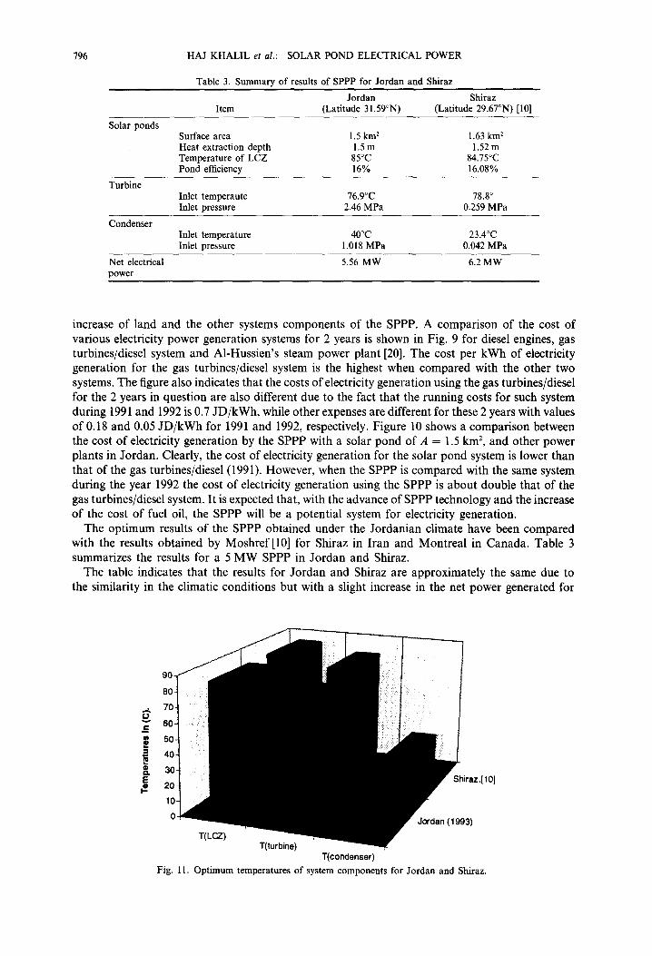
The optimum results of the SPPP obtained under the Jordanian climate have been compared with the results obtained by Moshref [lo] for Shiraz in Iran and Montreal in Canada. Table 3 summarizes the results for a 5 MW SPPP in Jordan and Shiraz.

The table indicates that the results for Jordan and Shiraz are approximately the same due to the similarity in the climatic conditions but with a slight increase in the net power generated for

2 70.

' .e 60-

I 50-

5 5 40-

z.(lO]

T(condenser) Fig. 11. Optimum temperatures of system components for Jordan and Shiraz.

HAJ KHALIL et al.: SOLAR POND ELECTRICAL POWER 197

s ‘i: e

Shim 1993($kWh)

g El > .f: .$

H Z z Jordan 1993(J.[YkWh) 'j s

0 0.05 0.1 0.15 0.2 0.25 0.3 0.35 0.4 0.45

Cost of electricity generation. Fig. 12. Cost of electricity generation using SPPP in Jordan and Shiraz.

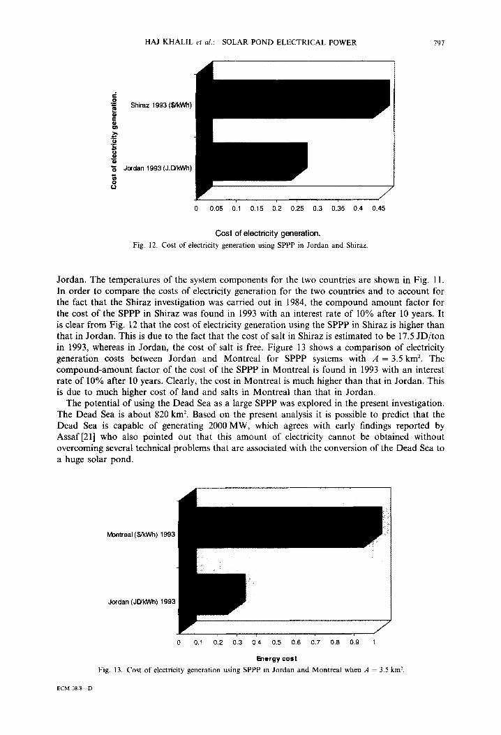
Jordan. The temperatures of the system components for the two countries are shown in Fig. 11. In order to compare the costs of electricity generation for the two countries and to account for the fact that the Shiraz investigation was carried out in 1984, the compound amount factor for the cost of the SPPP in Shiraz was found in 1993 with an interest rate of 10% after 10 years. It is clear from Fig. 12 that the cost of electricity generation using the SPPP in Shiraz is higher than that in Jordan. This is due to the fact that the cost of salt in Shiraz is estimated to be 17.5 JD/ton in 1993, whereas in Jordan, the cost of salt is free. Figure 13 shows a comparison of electricity generation costs between Jordan and Montreal for SPPP systems with A = 3.5 km2. The compound-amount factor of the cost of the SPPP in Montreal is found in 1993 with an interest rate of 10% after 10 years. Clearly, the cost in Montreal is much higher than that in Jordan. This is due to much higher cost of land and salts in Montreal than that in Jordan.

The potential of using the Dead Sea as a large SPPP was explored in the present investigation. The Dead Sea is about 820 km*. Based on the present analysis it is possible to predict that the Dead Sea is capable of generating 2000 MW, which agrees with early findings reported by Assaf [21] who also pointed out that this amount of electricity cannot be obtained without overcoming several technical problems that are associated with the conversion of the Dead Sea to a huge solar pond.

Montreal($kWh) 1993

Jordan(J[YkWh)1993

0 0.1 0.2 013 d.4 0.5 0.6 0.7 0.8 0.9 1

Energycost

Fig. 13. Cost of electricity generation using SPPP in Jordan and Montreal when A = 3.5 km?.

ECM 38/8-D

798 HAJ KHALIL et al.: SOLAR POND ELECTRICAL POWER

4. CONCLUSIONS Several points have emerged from the present work which can be summarized as follows:

Environmentally friendly refrigerants, such as R134a, can be used as the working fluid successfully with acceptable cost in organic cycles that are used with the SPPP. The electricity generation in Jordan using a solar pond in connection with an organic cycle is a rather good potential with relatively acceptable cost, especially when one considers future fuel prices as well as the advances in solar pond technology. Optimum sizing of system components of the SPPP is very much dependent on the climatic conditions, in particular the incident solar radiations.

Acknowledgements-The authors would like to thank the Jordanian Higher Research Council and the Jordanian Industrial Bank for sponsoring this work. The authors would also like to acknowledge the valuable assistance of the computer center staff at the Engineering and Technology Faculty at the University of Jordan.

REFERENCES 1. Y. L. Bronicki, IEEE Spectrum, Feb. 1981, 5659. 2. A. A. Badran, B. A. Jubran, E. M. Qasem and M. A. Hamdan, Submitted for publication. Journal Appl. Energy, 1995. 3. 2. Panahi, J. C. Batty and J. P. Riley, Journal of Solar Energy Engineering, ASME Transactions 1983, 105, 369. 4. H. Rubin and B. A. Benedict, Solar Energy, 1984, 32(32), 771. 5. R. S. Deriwul and R. Singh, Hear Recovery Systems & CHP, 1987, 7, 497. 6. H. Xe, P. Golding and C. E. Nielsen, Prediction of internal stability in a salt gradient solar pond, International Progress

in Solar Ponds Conference, Cuenavaca, Mexico, 1987. 7. H. Z. Tabor and B. Doron, The Beit Haarava 5 MWe solar pond power plant progress report, International Progress

in Solar Ponds Conference, Cuenavaca, Mexico, 1987. 8. Bectel Corporation, Technical and economic assessment of the prospects for electrical power generation by use of solar

ponds, Report to the U.S. Energy Research and Development Administration, Washington, D.C., pp. 1.1-6.3, August 1975.

9. A. Ophir and N. Nadav, Desalination, 1982, 40, 103. IO. A. Moshref A., Simulation and optimization of electric power generation by solar ponds, Ph.D. thesis, McGill

University, Canada, 1983. 11. E. Al-Qasem, Solar pond greenhouse heating system, Master Thesis, University of Jordan, Amman, Jordan, Dec. 1994. 12. S. A. Shah, T. H. Short and R. P. Flynn, Solar Energy, 1981, 27(5), 393. 13. H. C. Bryant and I. Colbeck, Solar Energy, 1977, 19, 321. 14. J. A. Duflie and W. A. Beckmen, Solar Engineering of Thermal Processes, Wiley-InterScience Publication, New York,

1980. 15. J. R. Hull, K. V. Liu and W. J. Sha, Dependence of ground heat losses upon solar pond size and parameter, Solar

Energy, 1984, 33, 25. 16. A. Arbel and M. Sokolov, ASME Trans. Solar Energy Engineering, 1991, 113, 66. 17. A. Rabel and C. E. Nielsen, Solar Energy, 1975, 17, 1. 18. D. Crevier, State of the art review of solar ponds, Solar Energy Project Report No. Pond-l, National Research Council

of Canada, August 1980. 19. R. A. Haj Khalil, Simulation and optimization of electrical power generation by solar ponds in Jordan, Master Thesis,

University of Jordan, Amman, Jordan, July 1995. 20. M. Asaad, Private Communication, Jordan Electricity Authority, 1995. 21. G. Assaf, Solar Energy, 1976, 18(4), 293.