Steady Currents

If at first you don’t succeed, try, try again. Then quit. No sense being a damn fool about it.

— W.C. Fields

Electric current: the slow average drift of chargeOne might think the discussion of charges in motion would begin with a description of the fields of a single moving point charge. But those fields are quite complicated — even if the charge is moving with constant velocity, but especially if it is accelerating.However, when we consider the average fields produced by a large number of identical charges moving (on average) relatively slowly, the situation is much simpler. Especially simple is the case where the charges move with constant average velocity. In that case, called direct current (DC), the flow of charge is much like that of mass in a perfect fluid.To describe the flow we introduce the electric current density:

Current density

Electric current density j is a vector field. Its direction is that of the flow of positive charge; its magnitude is equal to the amount of charge passing in unit time through unit area normal to the flow.

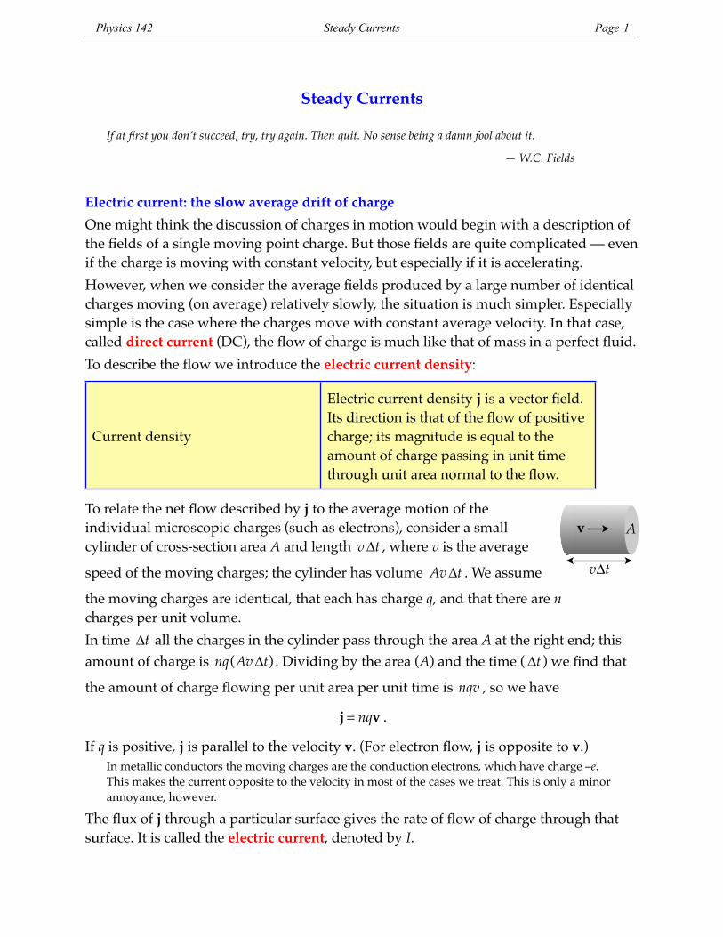
To relate the net flow described by j to the average motion of the individual microscopic charges (such as electrons), consider a small cylinder of cross-section area A and length vΔt , where v is the average

speed of the moving charges; the cylinder has volume AvΔt . We assume

the moving charges are identical, that each has charge q, and that there are n charges per unit volume.In time Δt all the charges in the cylinder pass through the area A at the right end; this amount of charge is nq(AvΔt) . Dividing by the area (A) and the time ( Δt ) we find that

the amount of charge flowing per unit area per unit time is nqv , so we have

j = nqv .

If q is positive, j is parallel to the velocity v. (For electron flow, j is opposite to v.)In metallic conductors the moving charges are the conduction electrons, which have charge –e. This makes the current opposite to the velocity in most of the cases we treat. This is only a minor annoyance, however.

The flux of j through a particular surface gives the rate of flow of charge through that surface. It is called the electric current, denoted by I.

vΔt

v A

Physics 142 Steady Currents Page 1

! !

Electric current as flux of current density I = j ⋅dA∫

In our applications the conductors will usually be in the form of wires, for which the surface in question is the cross-section of the wire. Then I is the the total amount of charge passing a particular point on the wire per unit time, which one often writes as

Electric current as charge passing by per unit time

I = dQdt

Electric current is measured in amperes (A). A current of 1 A means that 1 C of charge passes a point on the wire per second. This is a current of moderate size, about the amount passing through a 100 W incandescent light bulb.

The SI system of electrical units is in fact based on the ampere. One coulomb of charge is defined as the amount flowing in one second past a point in a wire carrying a current of one ampere.

Resistance: conversion of field energy to thermal energyWe have seen that charges in a conductor, left to themselves, quickly rearrange and come to rest in electrostatic equilibrium. To keep them moving requires continuous application of an external E-field. We will discuss below some possible sources of this external field. For now we will just assume such a field exists.For currents in ordinary conductors (not superconductors) a steady state is quickly reached, in which the energy given to the conduction electrons by the external E-field exactly balances the energy they lose in collisions with the “lattice” of atoms of which the material is made. This lost kinetic energy is manifested in the form of thermal energy of random motion of the lattice particles, a process called Joule heating.In this steady state there remains a small average velocity of the conduction electrons, called the “drift” velocity. This velocity (which is denoted by v in the discussion above) is in the direction of the force exerted by the external field. The current density j is parallel to E, and the relation between these vectors defines the resistivity of the material, a positive scalar denoted by ρ :

Resistivity E = ρj

For many common conducting materials and E-fields that are not too strong, ρ is approximately independent of E. This property is called Ohm's Law. Materials for which it is a good approximation are called “ohmic”.

This rule was discovered by Ohm in 1826. It was a significant finding, showing that the current in a circuit is proportional to the battery’s “tension,” as potential difference was called at that time.

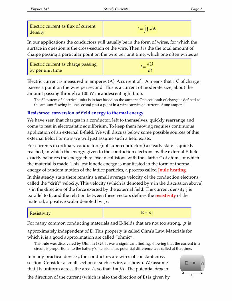
In many practical devices, the conductors are wires of constant cross-section. Consider a small section of such a wire, as shown. We assume that j is uniform across the area A, so that I = jA . The potential drop in

the direction of the current (which is also the direction of E) is given by ℓ

E A

Physics 142 Steady Currents Page 2

! !

ΔV = Eℓ . We find, using E = ρ j and j = I /A :

ΔV =

ρℓA

I .

The factor multiplying I in this equation is called the resistance. Its definition is:

Resistance

If steady current I passes through a passive element, resulting in potential drop ΔV between its ends, then the element has resistance R = ΔV /I .

A “passive” element is one that does not transfer energy into or out of the circuit except by means of its resistance; this excludes “active” elements such as batteries.

In this context, Ohm's Law is a statement that R is independent of ΔV and I.Here we have derived a useful formula for the resistance of a cylindrical conductor:

R =

ρℓA

.

The general formula for power input to a circuit elementFor any element through which current I passes, the amount of charge going in one end and out the other in time dt is given by dQ = I dt . If the potential drop between the ends

of the element is ΔV , then as this bit of charge passes through the element the system loses an amount of electrostatic potential energy dU = ΔV ⋅dQ , which is transformed into other kinds of energy. The rate at which this transformation occurs is given by

P = dU /dt = ΔV ⋅dQ/dt = I ΔV .

The current leaving the element is the same as that entering, so the speed of the charges does not change: there is no change in kinetic energy of their motion. The lost electrostatic potential energy is changed to other forms (e.g., heat), or transferred to other systems. There are many possibilities, some of which we will discuss as we go along. Regardless of where the energy goes, we have derived a simple and general formula for the amount of electrical power delivered to the element:

Power input to circuit element P = I ΔVIt is important that ΔV represents the drop in potential as the current passes through the element. If this drop is positive (the potential really does drop) then power is being delivered from the rest of the circuit to the element as electric field energy gets converted to other forms. If the drop is negative (the potential rises) then energy is being converted form other forms to electric field energy, and the element is providing power to the rest of the circuit.

In the case of an ordinary wire, in which the potential drop comes only from resistance, the energy input to the wire is converted into thermal energy by Joule heating. In this case, ΔV = IR , so we have a simple formula for that process:

Physics 142 Steady Currents Page 3

! !

Joule heating P = I2R

There are many practical applications of this direct conversion of electric energy into heat, such as incandescent light bulbs and electric space heaters.

Energy balance in a circuit: emf and the circuit equationTo maintain a steady current, there must be a supply of energy to replace that lost in Joule heating or in other energy transformations. The source of this energy maintains the E-field from which the charges draw their energy. Such a source is called a “seat of electromotive force” or simply an emf. Its energy can arise from many processes.

The strength of an emf is measured by the energy it provides per unit charge, so its unit is volts.

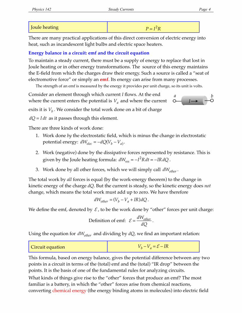
Consider an element through which current I flows. At the end where the current enters the potential is Va and where the current

exits it is Vb . We consider the total work done on a bit of charge

dQ = I dt as it passes through this element.

There are three kinds of work done:1. Work done by the electrostatic field, which is minus the change in electrostatic

potential energy: dWelec = −dQ(Vb −Va) .

2. Work (negative) done by the dissipative forces represented by resistance. This is given by the Joule heating formula: dWres = −I2Rdt = −IRdQ .

3. Work done by all other forces, which we will simply call dWother .

The total work by all forces is equal (by the work-energy theorem) to the change in kinetic energy of the charge dQ. But the current is steady, so the kinetic energy does not change, which means the total work must add up to zero. We have therefore

dWother = (Vb −Va + IR)dQ .

We define the emf, denoted by E , to be the work done by “other” forces per unit charge:

Definition of emf: E =

dWotherdQ

.

Using the equation for dWother and dividing by dQ, we find an important relation:

Circuit equation Vb −Va = E − IR

This formula, based on energy balance, gives the potential difference between any two points in a circuit in terms of the (total) emf and the (total) “IR drop” between the points. It is the basis of one of the fundamental rules for analyzing circuits.What kinds of things give rise to the “other” forces that produce an emf? The most familiar is a battery, in which the “other” forces arise from chemical reactions, converting chemical energy (the energy binding atoms in molecules) into electric field

a b I

Physics 142 Steady Currents Page 4

! !

energy. Various kinds of generators (such as the alternator in a car) convert mechanical energy of some kind—the engine in the car, falling water or steam driving a turbine, etc.—into electrical energy, often by use of Faraday's law, to be discussed later. Photocells of various kinds convert radiation into electric field energy. In all these devices, energy of a different sort is converted to electric field energy, producing an emf to sustain a current. In our applications in this section, the emf will be that of a battery.

DC circuits: Kirchhoff’s rulesA circuit is a system of elements connected by conductors in such a way that currents make complete round trips. In the process, electrical energy is brought in from emfs and transferred by means of the circuit to a “load” where it is converted into other forms, or perhaps passed on to other circuits.Here we analyze only circuits with currents that do not vary with time (DC). The sources of energy (emfs) will be batteries. The loads will be simple resistances.The two fundamental principles governing the circuit are:

• Energy balance, expressed by the circuit equation given above.• Conservation of charge.

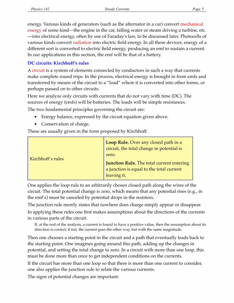
These are usually given in the form proposed by Kirchhoff:

Kirchhoff’s rules

Loop Rule. Over any closed path in a circuit, the total change in potential is zero.

Junction Rule. The total current entering a junction is equal to the total current leaving it.

One applies the loop rule to an arbitrarily chosen closed path along the wires of the circuit. The total potential change is zero, which means that any potential rises (e.g., in the emf’s) must be canceled by potential drops in the resistors.The junction rule merely states that nowhere does charge simply appear or disappear. In applying these rules one first makes assumptions about the directions of the currents in various parts of the circuit.

If, at the end of the analysis, a current is found to have a positive value, then the assumption about its direction is correct; if not, the current goes the other way, but with the same magnitude.

Then one chooses a starting point in the circuit and a path that eventually leads back to the starting point. One imagines going around this path, adding up the changes in potential, and setting the total change to zero. In a circuit with more than one loop, this must be done more than once to get independent conditions on the currents.If the circuit has more than one loop so that there is more than one current to consider, one also applies the junction rule to relate the various currents. The signs of potential changes are important:

Physics 142 Steady Currents Page 5

! !

• An emf crossed from its negative to its positive terminal gives an increase in potential. If it is crossed the other way it gives a decrease in potential.

• A resistance crossed in the direction of the current gives a decrease in potential of IR . If it is crossed against the current it give an increase in potential of IR .

We will illustrate these rules by some simple examples.

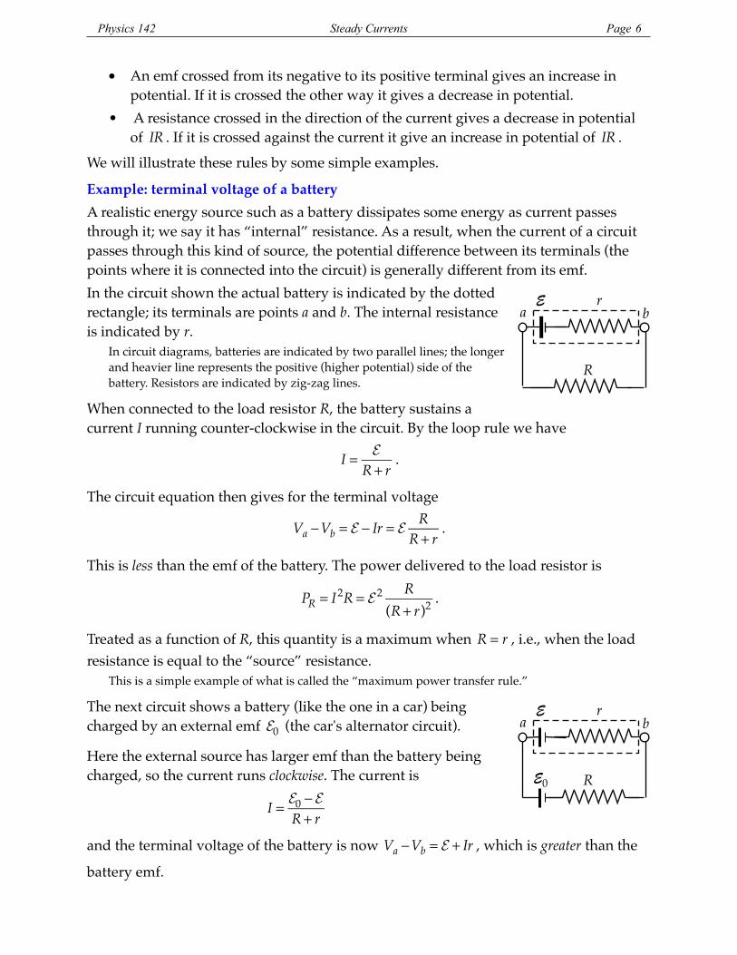
Example: terminal voltage of a batteryA realistic energy source such as a battery dissipates some energy as current passes through it; we say it has “internal” resistance. As a result, when the current of a circuit passes through this kind of source, the potential difference between its terminals (the points where it is connected into the circuit) is generally different from its emf.In the circuit shown the actual battery is indicated by the dotted rectangle; its terminals are points a and b. The internal resistance is indicated by r.

In circuit diagrams, batteries are indicated by two parallel lines; the longer and heavier line represents the positive (higher potential) side of the battery. Resistors are indicated by zig-zag lines.

When connected to the load resistor R, the battery sustains a current I running counter-clockwise in the circuit. By the loop rule we have

I = E

R + r.

The circuit equation then gives for the terminal voltage

Va −Vb = E − Ir = E

RR + r

.

This is less than the emf of the battery. The power delivered to the load resistor is

PR = I2R = E 2 R

(R + r)2 .

Treated as a function of R, this quantity is a maximum when R = r , i.e., when the load resistance is equal to the “source” resistance.

This is a simple example of what is called the “maximum power transfer rule.”

The next circuit shows a battery (like the one in a car) being charged by an external emf E0 (the car's alternator circuit).

Here the external source has larger emf than the battery being charged, so the current runs clockwise. The current is

I = E0 − E

R + r

and the terminal voltage of the battery is now Va −Vb = E + Ir , which is greater than the

battery emf.

a b r

R

E

a b r

R

E

E0

Physics 142 Steady Currents Page 6

! !

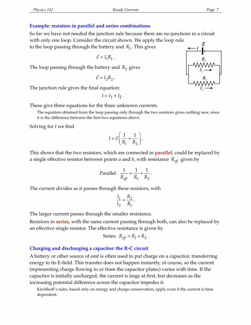
Example: resistors in parallel and series combinationsSo far we have not needed the junction rule because there are no junctions in a circuit with only one loop. Consider the circuit shown. We apply the loop rule to the loop passing through the battery and R1 . This gives

E = I1R1 .

The loop passing through the battery and R2 gives

E = I2R2 .

The junction rule gives the final equation:

I = I1 + I2 .

These give three equations for the three unknown currents. The equation obtained from the loop passing only through the two resistors gives nothing new, since it is the difference between the first two equations above.

Solving for I we find

I = E

1R1

+ 1R2

⎛⎝⎜

⎞⎠⎟

.

This shows that the two resistors, which are connected in parallel, could be replaced by a single effective resistor between points a and b, with resistance Reff given by

Parallel: 1

Reff= 1

R1+ 1

R2.

The current divides as it passes through these resistors, with

I1I2

=R2R1

.

The larger current passes through the smaller resistance.Resistors in series, with the same current passing through both, can also be replaced by an effective single resistor. The effective resistance is given by

Series: Reff = R1 + R2 .

Charging and discharging a capacitor: the R-C circuitA battery or other source of emf is often used to put charge on a capacitor, transferring energy to its E-field. This transfer does not happen instantly, of course, so the current (representing charge flowing to or from the capacitor plates) varies with time. If the capacitor is initially uncharged, the current is large at first, but decreases as the increasing potential difference across the capacitor impedes it.

Kirchhoff’s rules, based only on energy and charge conservation, apply even if the current is time dependent.

I

R1

I1R2

I2

E

Physics 142 Steady Currents Page 7

! !

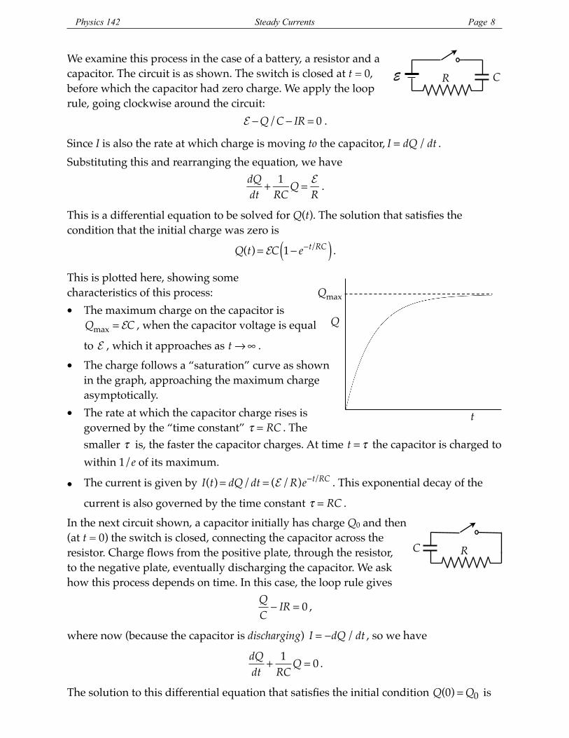
We examine this process in the case of a battery, a resistor and a capacitor. The circuit is as shown. The switch is closed at t = 0, before which the capacitor had zero charge. We apply the loop rule, going clockwise around the circuit:

E −Q/C − IR = 0 .

Since I is also the rate at which charge is moving to the capacitor, I = dQ / dt . Substituting this and rearranging the equation, we have

dQdt

+ 1RC

Q = E

R.

This is a differential equation to be solved for Q(t). The solution that satisfies the condition that the initial charge was zero is

Q(t) = EC 1− e−t/RC( ) .

This is plotted here, showing some characteristics of this process:• The maximum charge on the capacitor is

Qmax = EC , when the capacitor voltage is equal

to E , which it approaches as t →∞ .• The charge follows a “saturation” curve as shown

in the graph, approaching the maximum charge asymptotically.

• The rate at which the capacitor charge rises is governed by the “time constant” τ = RC . The smaller τ is, the faster the capacitor charges. At time t = τ the capacitor is charged to within 1/e of its maximum.

• The current is given by I(t) = dQ/dt = (E /R)e−t/RC . This exponential decay of the

current is also governed by the time constant τ = RC .In the next circuit shown, a capacitor initially has charge Q0 and then (at t = 0) the switch is closed, connecting the capacitor across the resistor. Charge flows from the positive plate, through the resistor, to the negative plate, eventually discharging the capacitor. We ask how this process depends on time. In this case, the loop rule gives

QC− IR = 0 ,

where now (because the capacitor is discharging) I = −dQ / dt , so we have

dQdt

+1

RCQ = 0 .

The solution to this differential equation that satisfies the initial condition Q(0) = Q0 is

C R E

Q

Qmax

t

C R

Physics 142 Steady Currents Page 8

! !

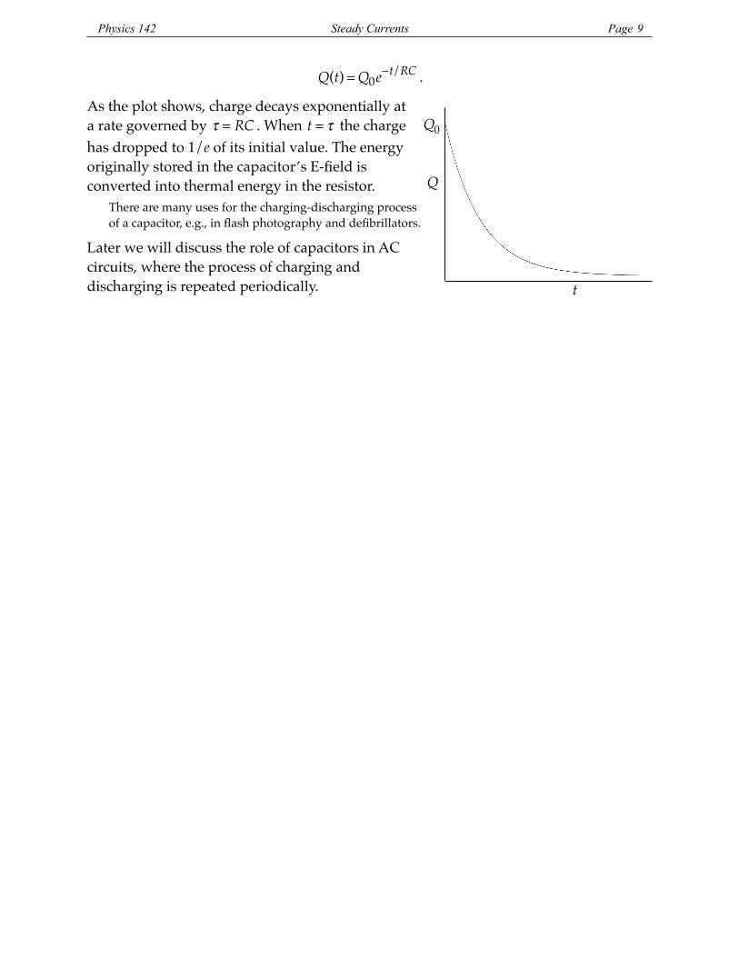
Q(t) = Q0e−t/RC .

As the plot shows, charge decays exponentially at a rate governed by τ = RC . When t = τ the charge has dropped to 1/e of its initial value. The energy originally stored in the capacitor’s E-field is converted into thermal energy in the resistor.

There are many uses for the charging-discharging process of a capacitor, e.g., in flash photography and defibrillators.

Later we will discuss the role of capacitors in AC circuits, where the process of charging and discharging is repeated periodically.

Q

Q0

t

Physics 142 Steady Currents Page 9

! !