Embed Size (px)
Citation preview
STEADY-STATE ANALYSIS OF REFLECTED
BROWNIAN MOTIONS: CHARACTERIZATION,
NUMERICAL METHODS AND QUEUEING APPLICATIONS
a dissertation
submitted to the department of mathematics
and the committee on graduate studies
of stanford university
in partial fulfillment of the requirements
for the degree of
doctor of philosophy
By
Jiangang Dai
July 1990

c© Copyright 2000 by Jiangang Dai
All Rights Reserved
ii
I certify that I have read this dissertation and that in my
opinion it is fully adequate, in scope and in quality, as a
dissertation for the degree of Doctor of Philosophy.
J. Michael Harrison(Graduate School of Business)
(Principal Adviser)
I certify that I have read this dissertation and that in my
opinion it is fully adequate, in scope and in quality, as a
dissertation for the degree of Doctor of Philosophy.
Joseph Keller
I certify that I have read this dissertation and that in my
opinion it is fully adequate, in scope and in quality, as a
dissertation for the degree of Doctor of Philosophy.
David Siegmund(Statistics)
Approved for the University Committee on Graduate Studies:
Dean of Graduate Studies
iii
Abstract
This dissertation is concerned with multidimensional diffusion processes that arise as ap-
proximate models of queueing networks. To be specific, we consider two classes of semi-
martingale reflected Brownian motions (SRBM’s), each with polyhedral state space. For
one class the state space is a two-dimensional rectangle, and for the other class it is the
general d-dimensional non-negative orthant Rd+.
SRBM in a rectangle has been identified as an approximate model of a two-station queue-
ing network with finite storage space at each station. Until now, however, the foundational
characteristics of the process have not been rigorously established. Building on previous
work by Varadhan and Williams [53] and by Taylor and Williams [50], we show how SRBM
in a rectangle can be constructed by means of localization. The process is shown to be
unique in law, and therefore to be a Feller continuous strong Markov process. Taylor and
Williams [50] have proved the analogous foundational result for SRBM in the non-negative
orthant Rd+, which arises as an approximate model of a d-station open queueing network
with infinite storage space at every station.
Motivated by the applications in queueing theory, our focus is on steady-state analy-
sis of SRBM, which involves three tasks: (a) determining when a stationary distribution
exists; (b) developing an analytical characterization of the stationary distribution; and (c)
computing the stationary distribution from that characterization. With regard to (a), we
give a sufficient condition for the existence of a stationary distribution in terms of Lia-
punov functions. With regard to (b), for a special class of SRBM’s in an orthant, Harrison
and Williams [26] showed that the stationary distribution must satisfy a weak form of an
adjoint linear elliptic partial differential equation with oblique derivative boundary condi-
tions, which they called the basic adjoint relationship (BAR). They further conjectured that
(BAR) characterizes the stationary distribution. We give two proofs of their conjecture.
For an SRBM in a rectangle, using Echeverria’s Theorem [10], we give a direct proof of their
iv
conjecture. For an SRBM in a general dimensional space, we first characterize an SRBM as
a solution to a constrained martingale problem. Then, using Kurtz’s recent theorem [32],
we prove their conjecture for general SRBM’s.
The most novel contribution of this dissertation relates to the computational task (c)
above. To make practical use of SRBM’s as approximate models of queueing networks, one
needs practical methods for determining stationary distributions, and it is very unlikely that
general analytical solutions will ever be found. We describe an approach to computation
of stationary distributions that seems to be widely applicable. That approach gives rise to
a family of algorithms, and we investigate one version of the algorithm. Under one mild
assumption, we are able to provide a full proof of the algorithm’s convergence. We compare
the numerical results from our algorithm with known analytical results for SRBM, and
also use the algorithm to estimate the performance measures of several illustrative open
queueing networks. All the numerical comparisons show that our method gives reasonably
accurate estimates and the convergence is relatively fast.
The algorithms that we have thus far implemented in computer code are quite limited
as tools for analysis of queueing systems, but the underlying computational approach is
widely applicable. Our ultimate goal is to implement this approach in a general routine for
computing the stationary distribution of SRBM in an arbitrary polyhedral state space. The
plan is to combine that routine with appropriate “front end” and “back end” program mod-
ules to form a software package, tentatively called QNET, for analysis of complex queueing
networks. This package would be much more widely applicable than the commercial pack-
ages currently available for performance analysis of queueing networks, such as PANACEA
[38] and QNA [54], but only the first tentative steps in its development have been taken
thus far.
v

Acknowledgments
I am grateful to my advisor, Professor Michael Harrison, for introducing me to reflected
Brownian motions and their connections with queueing theory, and for his advice and many
contributions to this dissertation. I am also grateful for his role in making the presentation
of this dissertation clearer.
I would like to thank Professor Ruth Williams in the Department of Mathematics,
University of California at San Diego, for her help throughout my graduate studies at
Stanford. She has been generous with her time and ideas, and has given me access to
her important current work with Lisa Taylor. In addition, Professor Williams has read
portions of this dissertation in preliminary draft form, always returning the manuscript
promptly, often with comments and corrections as extensive as the text itself. Her influence
is particularly apparent in Section 2.2.
I am grateful to Professor Thomas Kurtz in the Department of Mathematics and Statis-
tics, University of Wisconsin at Madison, for several valuable conversations while he was
visiting Stanford in the Spring of 1989. Before leaving Stanford, he wrote me a note that
basically provided a proof for Theorem 3.5. I am also grateful to Gary Lieberman in the
Department of Mathematics, Iowa State University, for many communications on elliptic
equations with oblique boundary conditions. Although many of the results he produced for
me are not quoted here, his generous help has been important.
I thank Stanford Professors Joseph Keller and David Siegmund for taking time to read
my dissertation, and Professor T. L. Lai for his guidance and encouragement in the early
stages of my career at Stanford.
My special thanks go to Professors Xuan-Da Hu and Hu-Mian Zhong at Nanjing Uni-
versity, and Professor Jia-An Yan at the Institute of Applied Mathematics, Academica
Sinica, for introducing me to the stochastic calculus, which plays an essential role in this
dissertation.
vi

I would like to thank my fellow students for proofreading parts of this dissertation, and
their friendship. Among them are Ken Dutch, David Ho, Christoph Loch, Vien Nguyen,
Mike Pich, Richard Tobias and Heping Zhang.
The final group of people whom I wish to thank for their support is my family: my
father, my sister, my late mother and my late brother. They have been a constant source
of emotional support throughout the years of my education. This dissertation is dedicated
to my beloved mother and brother.
Although many people have helped me along the way, none is more responsible for my
completing this dissertation than my wife, Li-Qin. Giving up a graduate study opportu-
nity in biochemistry, she came to Stanford and provided love, support, and understanding
through many disappointments which accompany accomplishments. Her support was par-
ticularly important during the difficult period when I lost my beloved brother at the end of
my first year at Stanford.
Thanks go to Stanford Mathematics Department and Graduate School of Business for
their financial support over the past four years.
vii
Contents
Abstract iv
Acknowledgments vi
List of Tables xi
List of Figures xiii
Frequently Used Notation xiv
1 Introduction 1
1.1 Motivation . . . . . . . . . . . . . . . . . . . . . . . . . . . . . . . . . . . . 1
1.2 A Tandem Queue . . . . . . . . . . . . . . . . . . . . . . . . . . . . . . . . . 3
1.3 Overview . . . . . . . . . . . . . . . . . . . . . . . . . . . . . . . . . . . . . 5
1.4 Notation and Terminology . . . . . . . . . . . . . . . . . . . . . . . . . . . . 7
2 SRBM in a Rectangle 9
2.1 Definition . . . . . . . . . . . . . . . . . . . . . . . . . . . . . . . . . . . . . 9
2.2 Existence and Uniqueness of an SRBM . . . . . . . . . . . . . . . . . . . . . 11
2.2.1 Construction of an RBM . . . . . . . . . . . . . . . . . . . . . . . . 11
2.2.2 Semimartingale Representation . . . . . . . . . . . . . . . . . . . . . 20
2.2.3 Uniqueness . . . . . . . . . . . . . . . . . . . . . . . . . . . . . . . . 26
2.3 Stationary Distribution . . . . . . . . . . . . . . . . . . . . . . . . . . . . . 30
2.3.1 The Basic Adjoint Relationship (BAR) . . . . . . . . . . . . . . . . 30
2.3.2 Sufficiency of (BAR)—A First Proof . . . . . . . . . . . . . . . . . . 31
2.4 Numerical Method for Steady-State Analysis . . . . . . . . . . . . . . . . . 34
viii
2.4.1 Inner Product Version of (BAR) and a Least Squares Problem . . . 34
2.4.2 An Algorithm . . . . . . . . . . . . . . . . . . . . . . . . . . . . . . 37
2.5 Numerical Comparisons . . . . . . . . . . . . . . . . . . . . . . . . . . . . . 39
2.5.1 Comparison with SC Solutions . . . . . . . . . . . . . . . . . . . . . 39
2.5.2 Comparison with Exponential Solutions . . . . . . . . . . . . . . . . 40
2.5.3 A Tandem Queue with Finite Buffers . . . . . . . . . . . . . . . . . 45
2.6 Concluding Remarks . . . . . . . . . . . . . . . . . . . . . . . . . . . . . . . 50
3 SRBM in an Orthant 52
3.1 Introduction and Definitions . . . . . . . . . . . . . . . . . . . . . . . . . . . 52
3.2 Feller Continuity and Strong Markov Property . . . . . . . . . . . . . . . . 54
3.3 Constrained Martingale Problem . . . . . . . . . . . . . . . . . . . . . . . . 58
3.4 Existence of a Stationary Distribution . . . . . . . . . . . . . . . . . . . . . 61
3.4.1 Necessary Conditions . . . . . . . . . . . . . . . . . . . . . . . . . . 61
3.4.2 A Sufficient Condition . . . . . . . . . . . . . . . . . . . . . . . . . . 63
3.5 The Basic Adjoint Relationship (BAR) . . . . . . . . . . . . . . . . . . . . . 66
3.5.1 Necessity of (BAR) . . . . . . . . . . . . . . . . . . . . . . . . . . . . 67
3.5.2 Sufficiency of (BAR)–A General Proof . . . . . . . . . . . . . . . . . 67
4 Computing the Stationary Distribution of SRBM in an Orthant 71
4.1 Introduction . . . . . . . . . . . . . . . . . . . . . . . . . . . . . . . . . . . . 71
4.2 An Inner Product Version of (BAR) . . . . . . . . . . . . . . . . . . . . . . 73
4.3 Algorithm . . . . . . . . . . . . . . . . . . . . . . . . . . . . . . . . . . . . . 74
4.4 Choosing a Reference Density and Hn . . . . . . . . . . . . . . . . . . . . 77
4.5 Numerical Comparisons . . . . . . . . . . . . . . . . . . . . . . . . . . . . . 81
4.5.1 A Two-Dimensional RBM . . . . . . . . . . . . . . . . . . . . . . . . 81
4.5.2 Symmetric RBM’s . . . . . . . . . . . . . . . . . . . . . . . . . . . . 82
4.6 Queueing Network Applications . . . . . . . . . . . . . . . . . . . . . . . . . 85
4.6.1 Queues in Series . . . . . . . . . . . . . . . . . . . . . . . . . . . . . 85
4.6.2 Analysis of a Multiclass Queueing Network . . . . . . . . . . . . . . 104
A Detailed Description of the Algorithm 108
A.1 Input Parameters and Scaling . . . . . . . . . . . . . . . . . . . . . . . . . . 108
A.2 Indexing . . . . . . . . . . . . . . . . . . . . . . . . . . . . . . . . . . . . . . 110
ix

A.3 Basis and Inner Product . . . . . . . . . . . . . . . . . . . . . . . . . . . . . 112
A.4 Stationary Density . . . . . . . . . . . . . . . . . . . . . . . . . . . . . . . . 113
A.5 “C” code for BNET . . . . . . . . . . . . . . . . . . . . . . . . . . . . . . . 115
Bibliography 125
x
List of Tables
2.1 Comparisons with SCPACK when n = 6 . . . . . . . . . . . . . . . . . . . . 41
2.2 Comparisons with Exponential Solutions when Γ = I and t3 = 0.0 . . . . . 45
2.3 Comparisons with Exponential Solutions when Γ = I and t3 = 0.5 . . . . . 46
2.4 Comparisons with Exponential Solutions when Γ = I and t3 = 1.0 . . . . . 46
2.5 Comparisons with Exponential Solutions when Γ = I and t3 = 1.5 . . . . . 46
2.6 Comparisons with Other Exponential Solutions when n = 6 . . . . . . . . . 47
2.7 Performance Estimates for the Queueing Model Pictured in Figure 2.2 . . . 49
4.1 Convergence of the Algorithm . . . . . . . . . . . . . . . . . . . . . . . . . . 82
4.2 QNET Estimates for m1 when d = 2 (n = 3) . . . . . . . . . . . . . . . . . 84
4.3 Relative Errors when d = 2 (n = 3) . . . . . . . . . . . . . . . . . . . . . . . 84
4.4 Relative Errors when d = 3 (n = 3) . . . . . . . . . . . . . . . . . . . . . . . 84
4.5 Relative Errors when d = 4 (n = 3) . . . . . . . . . . . . . . . . . . . . . . . 84
4.6 Comparisons with Fraker’s Experiments . . . . . . . . . . . . . . . . . . . . 88
4.7 Convergence of the Algorithm . . . . . . . . . . . . . . . . . . . . . . . . . . 88
4.8 Comparisons with Shimshak’s Experiment I . . . . . . . . . . . . . . . . . . 90
4.9 Comparisons with Shimshak’s Experiment III . . . . . . . . . . . . . . . . . 91
4.10 Comparisons with Shimshak’s Experiment IV . . . . . . . . . . . . . . . . . 92
4.11 Expected Waiting Times at the Second Queue: Case 1 . . . . . . . . . . . . 96
4.12 Expected Waiting Times at the Second Queue: Case 2 . . . . . . . . . . . . 97
4.13 Expected Waiting Times at the Second Queue: Case 3 . . . . . . . . . . . . 98
4.14 Expected Waiting Times at the Second Queue: Case 4 . . . . . . . . . . . . 99
4.15 Expected Waiting Times at the Second Queue: Case 5 . . . . . . . . . . . . 100
4.16 Expected Waiting Times at the Second Queue: Case 6 . . . . . . . . . . . . 101
4.17 Expected Waiting Times at the Second Queue: Case 7 . . . . . . . . . . . . 102
xi

4.18 Overall Comparisons with QNA Approximations in Heavy Traffic . . . . . . 103
4.19 Parameters for the Multiclass Queueing Network . . . . . . . . . . . . . . . 106
4.20 Mean Number of Customers for the Network Represented in Figure 4.2 . . 107
xii
List of Figures
1.1 Two Queues in Tandem . . . . . . . . . . . . . . . . . . . . . . . . . . . . . 3
1.2 State Space and Directions of Reflection for the Approximating SRBM . . . 4
2.1 State Space S and Directions of Reflection of an SRBM in a Rectangle . . . 9
2.2 Finite Queues in Tandem . . . . . . . . . . . . . . . . . . . . . . . . . . . . 47
2.3 State Space and Directions of Reflection for the Approximating SRBM . . . 48
3.1 State Space and Directions of Reflection of an SRBM when d = 2 . . . . . . 52
4.1 A Network of d Queues in Series . . . . . . . . . . . . . . . . . . . . . . . . 85
4.2 Model of an Interactive Computer . . . . . . . . . . . . . . . . . . . . . . . 104
xiii
Frequently Used Notation
I. Topological Notation. Let X be a subset of the d-dimensional Euclidean Space Rd.
1. X is the closure of X ⊂ Rd.
2. ∂X is the boundary of X ⊂ Rd.
3. BX is the Borel field of subsets of X.
4. Cb(X) is the set of bounded continuous functions f : X → R.
5. B(X) is the set of bounded BX -measurable f : X → R.
6. B(X) is the set of BX -measurable f : X → R.
7. P(X) is the set of probability measures on (X,BX).
8. ||f || ≡ supx∈X |f(x)| for f ∈ B(X).
9. CK(X) is the set of f ∈ Cb(X) having compact support.
10. Cmb (X) is the set of f : A → R possessing bounded derivatives of order up to
and including m for some open set A containing X.
11. CmK (X) ≡ Cmb (X) ∩ CK(X).
12. C0(X) is the set of f ∈ Cb(X) with limx→∞ f(x) = 0, see page 63.
II. Special Notation for Euclidean Space
1. x ∈ Rd is understood as a column vector.
2. |x| ≡ (∑di=1 x
2i )
1/2 for x ∈ Rd.
3. B(x, r) ≡ y ∈ Rd : |x− y| < r.
4. Rd+ ≡ x = (x1, . . . , xd)′ ∈ Rd, xi ≥ 0, i = 1, . . . , d.
5. 〈x, y〉 ≡∑di=1 xiyi for x, y ∈ Rd; x · y ≡ 〈x, y〉 for x, y ∈ Rd.
xiv
III. State Space and Path Space Notation for Reflected Brownian Motion
1. S is the state space, either a two-dimensional rectangle or the orthant Rd+.
2. O is the interior of S.
3. Fi is the ith face of boundary ∂S.
4. vi is a d-dimensional vector on face Fi, direction of reflection on Fi.
5. Γ is a d× d positive definite matrix, the covariance matrix.
6. µ is a d-dimensional vector, the drift vector.
7. R is a matrix whose columns are the vectors vi, the reflection matrix.
8. dx is Lebesgue measure on S.
9. dσi is Lebesgue measure on boundary face Fi.
10. ∇ is the gradient operator.
11. Dif ≡ vi · ∇f .
12. Gf = 12
∑di,j=1 Γij ∂2f
∂xi∂xj+∑di=1 µi
∂f∂xi
.
13. Af , see page 34 and page 73.
14. dλ, see page 34 and page 73.
15. dη, see page 74.
16. CS ≡ ω : [0,∞)→ S, ω is continuous .
17. ω is a generic element of CS .
18. Z = Z(t, ·), t ≥ 0 is the canonical process on CS , where Z(t, ω) ≡ ω(t), ω ∈ CS .
19. Mt ≡ σZ(s), 0 ≤ s ≤ t.
20. M≡ σZ(s), 0 ≤ s <∞.
IV. Miscellaneous Notation and Terminology
1. ⇒ weak convergence, see page 29.
2. ≈ equivalence of measures, see page 30.
3. .= approximate equality.
4. A′ is the transpose of a matrix A.
5. completely-S matrix, see Definition 3.4.
xv

6. Minkowski matrix, see Definition 3.3.
7. inf ∅ = +∞ and sup ∅ = 0, where ∅ is the empty set.
8. σ(C), where C is a set of functions on X into a measurable space, is the smallest
σ-algebra over X with respect to which every element of C is measurable.
9. r · q not an inner product, see page 73.
10. Ei: Erlang distribution.
11. M : exponential distribution.
12. D: deterministic distribution.
13. Hk: hyperexponential distribution.
V. Abbreviations
1. RBM—reflected Brownian motion, see page 11.
2. SRBM— semimartingale reflected Brownian motion, see page 9 and page 53.
3. (BAR)—basic adjoint relationship, see (2.35) and (3.30).
4. SCV— squared coefficient of variation (variance over squared mean).
5. QNA—queueing network analyzer, see page v.
6. QNET, see page v.
7. SIM—simulation estimate.
xvi
Chapter 1
Introduction
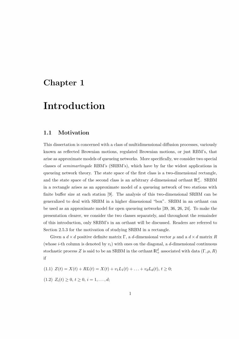
1.1 Motivation
This dissertation is concerned with a class of multidimensional diffusion processes, variously
known as reflected Brownian motions, regulated Brownian motions, or just RBM’s, that
arise as approximate models of queueing networks. More specifically, we consider two special
classes of semimartingale RBM’s (SRBM’s), which have by far the widest applications in
queueing network theory. The state space of the first class is a two-dimensional rectangle,
and the state space of the second class is an arbitrary d-dimensional orthant Rd+. SRBM
in a rectangle arises as an approximate model of a queueing network of two stations with
finite buffer size at each station [9]. The analysis of this two-dimensional SRBM can be
generalized to deal with SRBM in a higher dimensional “box”. SRBM in an orthant can
be used as an approximate model for open queueing networks [39, 36, 26, 24]. To make the
presentation clearer, we consider the two classes separately, and throughout the remainder
of this introduction, only SRBM’s in an orthant will be discussed. Readers are referred to
Section 2.5.3 for the motivation of studying SRBM in a rectangle.
Given a d× d positive definite matrix Γ, a d-dimensional vector µ and a d× d matrix R
(whose i-th column is denoted by vi) with ones on the diagonal, a d-dimensional continuous
stochastic process Z is said to be an SRBM in the orthant Rd+ associated with data (Γ, µ,R)
if
(1.1) Z(t) = X(t) +RL(t) = X(t) + v1L1(t) + . . .+ vdLd(t), t ≥ 0;
(1.2) Zi(t) ≥ 0, t ≥ 0, i = 1, . . . , d;
1
CHAPTER 1. INTRODUCTION 2
(1.3) X = X(t) is a d-dimensional Brownian motion with covariance matrix Γ and drift
vector µ;
(1.4) For i = 1, . . . , d, Li(0) = 0, Li is non-decreasing and Li(·) increases only at times t
such that Zi(t) = 0.
This definition suggests that the SRBM Z behaves like an ordinary Brownian motion with
covariance matrix Γ and drift vector µ in the interior of the orthant. When Z hits the
boundary xi = 0, the process (local time) Li(·) increases, causing an overall pushing in
the direction vi. The magnitude of the pushing is the minimal amount required to keep Z
inside the orthant.
The motivation for our study of SRBM in an orthant comes from the theory of open
queueing networks, that is, networks of interacting processors or service stations where cus-
tomers arrive from outside, visit one or more stations, perhaps repeatedly, in an order that
may vary from one customer to the next, and then depart. (In contrast, a closed queueing
network is one where a fixed customer population circulates perpetually through the sta-
tions of the network, with no new arrivals and no departures.) It was shown by Reiman
[39] that the d-dimensional queue length process associated with a certain type of open
d-station network, if properly normalized, converges under “heavy traffic” conditions to a
corresponding SRBM with state space Rd+. Peterson [36] proved a similar “heavy traffic
limit theorem” for open queueing networks with multiple customer types and deterministic,
feedforward customer routing; Peterson’s assumptions concerning the statistical distribu-
tion of customer routes are in some ways more general and in some ways more restrictive
than Reiman’s. The upshot of this work on limit theorems is to show that SRBM’s with
state space Rd+ may serve as good approximations, at least under heavy traffic conditions,
for the queue length processes, the workload processes, and the waiting time processes as-
sociated with various types of open d-station networks. Recently Harrison and Nguyen [24]
have defined a very general class of open queueing networks and articulated a systematic
procedure for approximating the associated stochastic processes by SRBM’s. This general
approximation scheme subsumes those suggested by the limit theorems of both Reiman and
Peterson, but it has not yet been buttressed by a rigorous and equally general heavy traffic
limit theory.
CHAPTER 1. INTRODUCTION 3
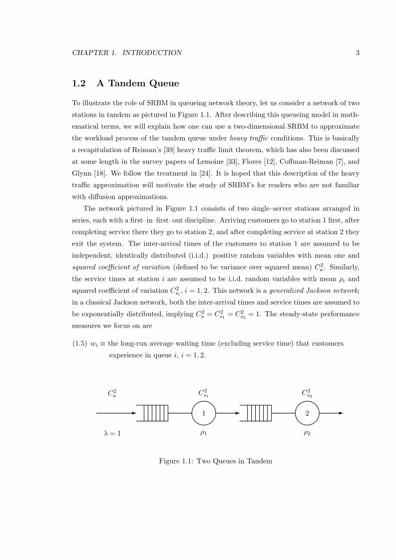
1.2 A Tandem Queue
To illustrate the role of SRBM in queueing network theory, let us consider a network of two
stations in tandem as pictured in Figure 1.1. After describing this queueing model in math-
ematical terms, we will explain how one can use a two-dimensional SRBM to approximate
the workload process of the tandem queue under heavy traffic conditions. This is basically
a recapitulation of Reiman’s [39] heavy traffic limit theorem, which has also been discussed
at some length in the survey papers of Lemoine [33], Flores [12], Coffman-Reiman [7], and
Glynn [18]. We follow the treatment in [24]. It is hoped that this description of the heavy
traffic approximation will motivate the study of SRBM’s for readers who are not familiar
with diffusion approximations.
The network pictured in Figure 1.1 consists of two single–server stations arranged in
series, each with a first–in–first–out discipline. Arriving customers go to station 1 first, after
completing service there they go to station 2, and after completing service at station 2 they
exit the system. The inter-arrival times of the customers to station 1 are assumed to be
independent, identically distributed (i.i.d.) positive random variables with mean one and
squared coefficient of variation (defined to be variance over squared mean) C2a . Similarly,
the service times at station i are assumed to be i.i.d. random variables with mean ρi and
squared coefficient of variation C2si , i = 1, 2. This network is a generalized Jackson network;
in a classical Jackson network, both the inter-arrival times and service times are assumed to
be exponentially distributed, implying C2a = C2
s1 = C2s2 = 1. The steady-state performance
measures we focus on are
(1.5) wi ≡ the long-run average waiting time (excluding service time) that customers
experience in queue i, i = 1, 2.
C2a
-
λ = 1
C2s1
"!#
1
ρ1
-
C2s2
"!#
2
ρ2
-
Figure 1.1: Two Queues in Tandem
CHAPTER 1. INTRODUCTION 4
When ρi < 1 (i = 1, 2), it is known that the network is stable (or ergodic), that is, wi <∞.
Despite its apparent simplicity, the tandem queue described above is not amenable to
exact mathematical analysis, except for the Jackson network case. But as an alternative
to simulation one may proceed with the following approximate analysis. Let Wi(t) be the
current workload at time t for server i, that is, the sum of the impending service times for
customers waiting at station i at time t, plus the remaining service time for the customer
currently in service there (if any). One can also think of Wi(t) as a virtual waiting time: if a
customer arrived at station i at time t, this customer would have to wait Wi(t) units of time
before gaining access to server i. The tandem queue is said to be in heavy traffic if ρ1 and
ρ2 are both close to one, and the heavy traffic limit theory referred to earlier suggests that
under such conditions the workload process W (t) can be well approximated by an SRBM
with state space R2+ and certain data (Γ, µ,R). To be more specific, Harrison and Nguyen
[24] propose that W (t) be approximated by an SRBM Z(t) with data
Γ =
ρ21(C2
a + C2s1) −ρ1ρ2C
2s1
−ρ1ρ2C2s1 ρ2
2(C2s1 + C2
s2)
, µ =
ρ1 − 1
ρ2/ρ1 − 1
, R =
1 0
−ρ2/ρ1 1,
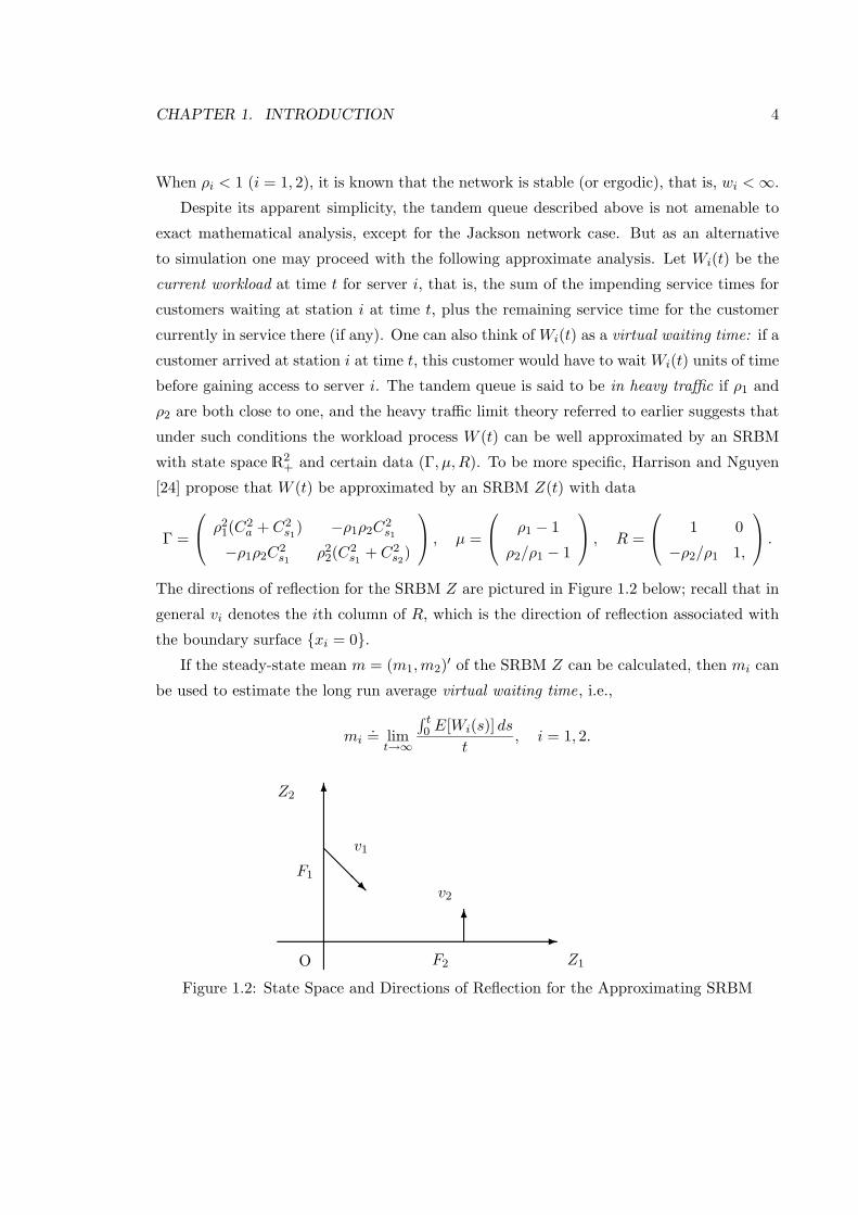
.The directions of reflection for the SRBM Z are pictured in Figure 1.2 below; recall that in
general vi denotes the ith column of R, which is the direction of reflection associated with
the boundary surface xi = 0.If the steady-state mean m = (m1,m2)′ of the SRBM Z can be calculated, then mi can
be used to estimate the long run average virtual waiting time, i.e.,
mi.= limt→∞
∫ t0 E[Wi(s)] ds
t, i = 1, 2.
-
6
O Z1
Z2
@@@R
v1
F1
6
v2
F2
Figure 1.2: State Space and Directions of Reflection for the Approximating SRBM
CHAPTER 1. INTRODUCTION 5
It is suggested in [24] that this long run average virtual waiting time be used to estimate the
long run average waiting time wi, i.e., wi.= mi (i = 1, 2). Notice that the SRBM uses only
the first two moments of the primitive queueing network data. This is typical of “Brownian
approximations”. In this dissertation we will focus on the analysis of an SRBM instead of
the original queueing network model.
1.3 Overview
There is now a substantial literature on Brownian models of queueing networks, and virtu-
ally all papers in that literature are devoted to one or more of the following tasks.
(a) Identify the Brownian analogs for various types of conventional queueing models, ex-
plaining how the data of the approximating SRBM are determined from the structure
and the parameters of the conventional model; prove limit theorems that justify the
approximation of conventional models by their Brownian analogs under “heavy traffic”
conditions.
(b) Show that the SRBM exists and is uniquely determined by an appropriate set of
axiomatic properties.
(c) Determine the analytical problems that must be solved in order to answer probabilistic
questions associated with the SRBM. These are invariably partial differential equation
problems (PDE problems) with oblique derivative boundary conditions. A question
of central importance, given the queueing applications that motivate the theory, is
which PDE problem one must solve in order to determine the stationary distribution
of an SRBM.
(d) Solve the PDE problems of interest, either analytically or numerically.
Most research to date has been aimed at questions (a) through (c) above. Topic (a) has been
discussed in Section 1.2 above. With regard to (b), Harrison and Reiman [25] proved, using
a unique path-to-path mapping, the existence and uniqueness of SRBM in an orthant when
the reflection matrix R is a Minkowski matrix (see Definition 3.3). This class of SRBM’s
corresponds to open queueing networks with homogeneous customer populations, which
means that customers occupying any given node or station of the network are essentially
indistinguishable from one another. Recently Taylor and Williams [50] proved the existence
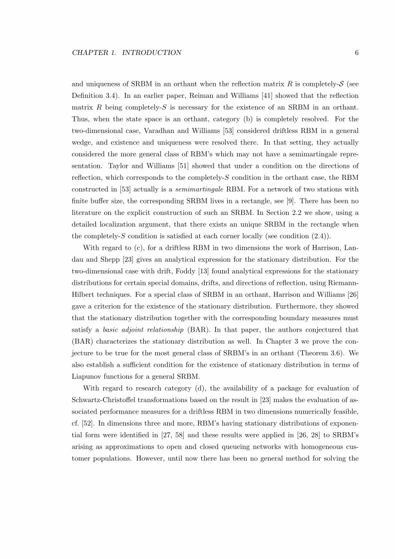
CHAPTER 1. INTRODUCTION 6
and uniqueness of SRBM in an orthant when the reflection matrix R is completely-S (see
Definition 3.4). In an earlier paper, Reiman and Williams [41] showed that the reflection
matrix R being completely-S is necessary for the existence of an SRBM in an orthant.
Thus, when the state space is an orthant, category (b) is completely resolved. For the
two-dimensional case, Varadhan and Williams [53] considered driftless RBM in a general
wedge, and existence and uniqueness were resolved there. In that setting, they actually
considered the more general class of RBM’s which may not have a semimartingale repre-
sentation. Taylor and Williams [51] showed that under a condition on the directions of
reflection, which corresponds to the completely-S condition in the orthant case, the RBM
constructed in [53] actually is a semimartingale RBM. For a network of two stations with
finite buffer size, the corresponding SRBM lives in a rectangle, see [9]. There has been no
literature on the explicit construction of such an SRBM. In Section 2.2 we show, using a
detailed localization argument, that there exists an unique SRBM in the rectangle when
the completely-S condition is satisfied at each corner locally (see condition (2.4)).
With regard to (c), for a driftless RBM in two dimensions the work of Harrison, Lan-
dau and Shepp [23] gives an analytical expression for the stationary distribution. For the
two-dimensional case with drift, Foddy [13] found analytical expressions for the stationary
distributions for certain special domains, drifts, and directions of reflection, using Riemann-
Hilbert techniques. For a special class of SRBM in an orthant, Harrison and Williams [26]
gave a criterion for the existence of the stationary distribution. Furthermore, they showed
that the stationary distribution together with the corresponding boundary measures must
satisfy a basic adjoint relationship (BAR). In that paper, the authors conjectured that
(BAR) characterizes the stationary distribution as well. In Chapter 3 we prove the con-
jecture to be true for the most general class of SRBM’s in an orthant (Theorem 3.6). We
also establish a sufficient condition for the existence of stationary distribution in terms of
Liapunov functions for a general SRBM.
With regard to research category (d), the availability of a package for evaluation of
Schwartz-Christoffel transformations based on the result in [23] makes the evaluation of as-
sociated performance measures for a driftless RBM in two dimensions numerically feasible,
cf. [52]. In dimensions three and more, RBM’s having stationary distributions of exponen-
tial form were identified in [27, 58] and these results were applied in [26, 28] to SRBM’s
arising as approximations to open and closed queueing networks with homogeneous cus-
tomer populations. However, until now there has been no general method for solving the
CHAPTER 1. INTRODUCTION 7
PDE problems alluded to in (d).
If Brownian system models are to have an impact in the world of practical performance
analysis, task (d) above is obviously crucial. In particular, practical methods are needed
for determining stationary distributions, and it is very unlikely that general analytical so-
lutions will ever be found. Thus we are led to the problem of computing the stationary
distribution of RBM in an orthant, or at least computing summary statistics of the sta-
tionary distribution. As we will explain later, the stationary distribution is the solution of
a certain highly structured partial differential equation problem (an adjoint PDE problem
expressed in weak form). In this dissertation, we describe an approach to computation of
stationary distributions that seems to be widely applicable. The method will be developed
and tested for two–dimensional SRBM’s with a rectangular state space in Section 2.4.2
through Section 2.5.3, and for higher dimensional SRBM’s in an orthant in Chapter 4. We
should point out that the proof of convergence would be complete if we could prove that
any solution to (BAR) does not change sign (see Conjecture 2.1 and Conjecture 4.1). As
readers will see, the method we use actually gives rise to a family of converging algorithms.
One particular implementation of our algorithm is tested against known analytical results
for SRBM’s as well as simulation results for queueing network models. The testing results
show that both the accuracy and speed of convergence are impressive for small networks.
We must admit that, currently, we do not have a general method to choose one “best”
algorithm from this family. In Appendix A, we will describe in detail how to implement
the version of the algorithm we use in the orthant case. As a tool for analysis of queueing
systems, the computer program described in this dissertation is obviously limited in scope,
but our ultimate goal is to implement the same basic computational approach in a general
routine that can compete with software packages like PANACEA [38] and QNA [54] in the
analysis of large, complicated networks.
1.4 Notation and Terminology
Here and later the symbol “≡” means “equals by definition”. We assume some basic notation
and terminology in probability as in Billingsley [4]. We denote the characteristic function
of a set A by 1A, i.e., 1A(x) = 1 if x ∈ A and 1A(x) = 0 otherwise. For a random variable
X and an event set A, we use E[X;A] to denote E[X1A]. Given a filtered probability space
(Ω,F , Ft, P ), a real-valued process X = X(t), t ≥ 0 defined on this space is said to be
CHAPTER 1. INTRODUCTION 8
adapted if for each t ≥ 0, X(t) is Ft-measurable. The process X is said to be an Ft-(sub)martingale under P if X is adapted, EP [|X(t)|] <∞ for each t ≥ 0 and for each pair
0 ≤ s < t and each A ∈ Fs, EP [X(s);A](≤) = EP [X(t);A], where EP is the expectation
with respect to the probability measure P .
The following are used extensively in the sequel. d ≥ 1 is an integer. S always denotes
a state space, either a two-dimensional rectangle or a d-dimensional orthant Rd+ ≡ x =
(x1, x2, . . . , xd)′ ∈ Rd : xi ≥ 0, i = 1, 2, . . . , d, where the prime is the transpose operator.
If no dimensionality is explicitly specified, a vector and a process are considered to be
d-dimensional. Vectors are treated as column vectors. Inequalities involving matrices or
vectors are interpreted componentwise. The set of continuous functions ω : [0,∞) → S is
denoted by CS . The canonical process on CS is Z = Z(t, ·), t ≥ 0 defined by
Z(t, ω) = ω(t), for ω ∈ CS .
The symbol ω is often suppressed in Z. The natural filtration associated with CS is Mt,where Mt ≡ σZ(s, ·) : 0 ≤ s ≤ t, t ≥ 0. For t ≥ 0, Mt can also be characterized as the
smallest σ-algebra of subsets of CS which makes Z(s) measurable for each 0 ≤ s ≤ t. The
natural σ-algebra associated with CS is M≡σZ(s, ·) : 0 ≤ s < ∞ =∨∞t=0Mt (
∨∞t=0Mt
is defined to be the smallest σ-algebra containing Mt for each t ≥ 0). For commonly used
notation, readers are referred to “Frequently Used Notation” on page xiv. Other notation
and terminology will be introduced as we proceed.
Chapter 2
SRBM in a Rectangle
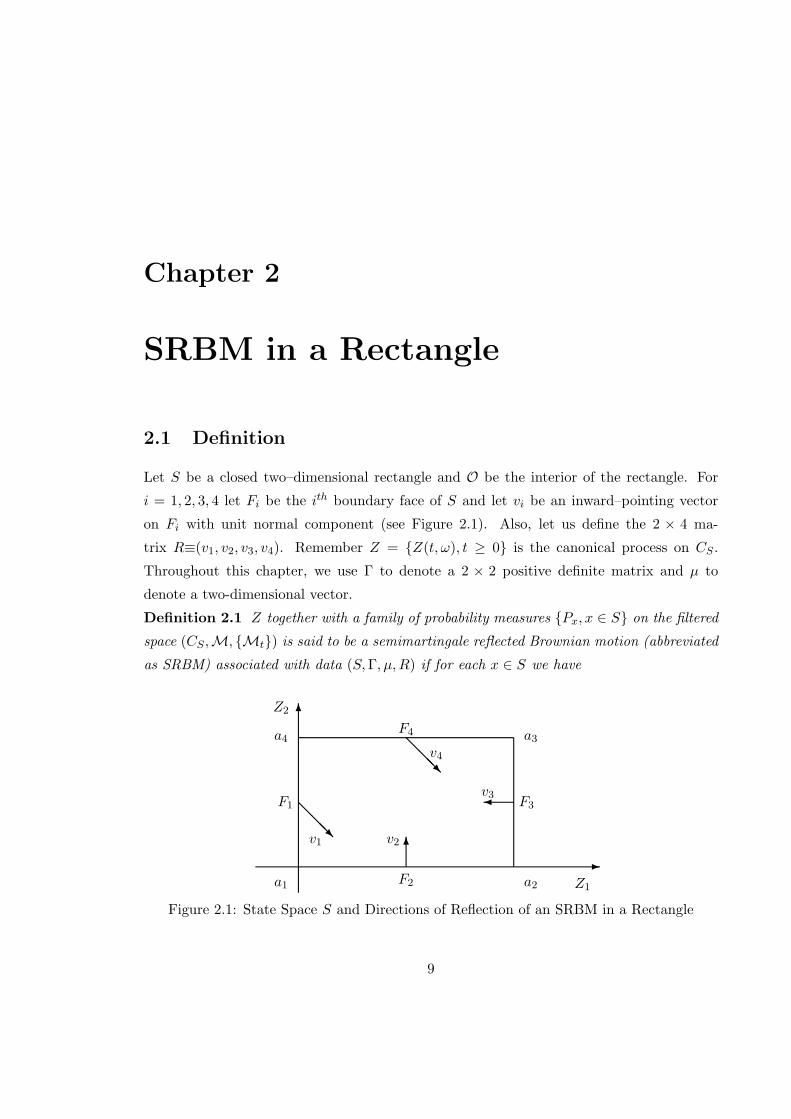
2.1 Definition
Let S be a closed two–dimensional rectangle and O be the interior of the rectangle. For
i = 1, 2, 3, 4 let Fi be the ith boundary face of S and let vi be an inward–pointing vector
on Fi with unit normal component (see Figure 2.1). Also, let us define the 2 × 4 ma-
trix R≡(v1, v2, v3, v4). Remember Z = Z(t, ω), t ≥ 0 is the canonical process on CS .
Throughout this chapter, we use Γ to denote a 2 × 2 positive definite matrix and µ to
denote a two-dimensional vector.
Definition 2.1 Z together with a family of probability measures Px, x ∈ S on the filtered
space (CS ,M, Mt) is said to be a semimartingale reflected Brownian motion (abbreviated
as SRBM) associated with data (S,Γ, µ,R) if for each x ∈ S we have
-
6
a1 Z1
Z2
a2
a4 a3
@@@Rv1
F1
6v2
F2
v3F3
@@@Rv4
F4
Figure 2.1: State Space S and Directions of Reflection of an SRBM in a Rectangle
9
CHAPTER 2. SRBM IN A RECTANGLE 10
(2.1) Z(t) = X(t) +RL(t) = X(t) +∑4i=1 viLi(t) ∀t ≥ 0, Px-a.s., where
(2.2) X(0) = x Px-a.s. and X is a 2-dimensional Brownian motion with covariance matrix
Γ and drift vector µ such that X(t)− µt,Mt, t ≥ 0 is a martingale under Px, and
(2.3) L is a continuous Mt-adapted four-dimensional process such that L(0) = 0, L
is non-decreasing, and Px-almost surely Li can increase only at times t such that
Z(t) ∈ Fi, i = 1, 2, 3, 4.
An SRBM Z as defined above behaves like a two-dimensional Brownian motion with drift
vector µ and covariance matrix Γ in the interior O of its state space. When the boundary
face Fi is hit, the process Li (sometimes called the local time of Z on Fi) increases, causing
an instantaneous displacement of Z in the direction given by vi; the magnitude of the
displacement is the minimal amount required to keep Z always inside S. Therefore, we
call Γ, µ and R the covariance matrix, the drift vector and the reflection matrix of Z,
respectively.
SRBM in a rectangle can be used as an approximate model of a two station queueing
network with finite buffer sizes at each station. Readers are referred to Section 2.5.3 and
[9] for more details.
Throughout this dissertation, when the state space S is a rectangle, we always assume
the given directions of reflection satisfy the following condition:
(2.4) there are positive constants ai and bi such that aivi + bivi+1 points into the interior
of S from the vertex where Fi and Fi+1 meet (i = 1, 2, 3, 4), where v5≡v1 and F5≡F1.
Because a Brownian motion can reach every region in the plane, it can be proved as in
Reiman and Williams [41] that (2.4) is a necessary condition for the existence of an SRBM.
In the following section, we will prove that there is a unique family Px, x ∈ S on (CS ,M)
such that Z together with Px, x ∈ S is an SRBM when the columns of the reflection
matrix R satisfy (2.4).
Definition 2.2 An SRBM Z is said to be unique (in law) if the corresponding family of
probability measures Px, x ∈ S is unique.
CHAPTER 2. SRBM IN A RECTANGLE 11
2.2 Existence and Uniqueness of an SRBM
Theorem 2.1 Let there be given a rectangle S, a non-degenerate covariance matrix Γ, a
drift vector µ and a reflection matrix R whose columns satisfy (2.4). Then there is a unique
family of probability measures Px, x ∈ S on (CS ,M, Mt) such that the canonical process
Z together with Px, x ∈ S is an SRBM associated with the data (S,Γ, µ,R). Furthermore,
the family Px, x ∈ S is Feller continuous, i.e., x → Ex[f(Z(t))] is a continuous for all
f ∈ Cb(S) and t ≥ 0, and Z together with Px, x ∈ S is a strong Markov process. Moreover,
supx∈S Ex[Li(t)] <∞ for each t ≥ 0 and i = 1, 2, 3, 4.
Remark. In this chapter, Ex is the expectation operator associated with the unique prob-
ability measure Px. We leave the proof of this theorem to the end of Section 2.2.3. To
this end, we first consider a class of reflected Brownian motions (RBM’s) as solutions to
certain submartingale problems as considered in Varadhan and Williams [53]. The main
difference between an RBM and an SRBM is that an RBM may not have a semimartin-
gale representation as in (2.1). When µ = 0, the authors in [53] showed the existence and
uniqueness of an RBM in a wedge for Γ = I, which immediately implies the existence and
uniqueness of an RBM in a quadrant with general non-degenerate covariance matrix Γ. In
Section 2.2.1, taking four RBM’s in four appropriate quadrants, we will carry out a detailed
patching argument to construct an RBM in the rectangle S. In Section 2.2.2, we show when
the reflection matrix R satisfies (2.4) that such an RBM actually has the semimartingale
representation (2.1). For µ 6= 0, the existence of an SRBM follows from that for µ = 0 and
Girsanov’s Theorem. Finally, in Section 2.2.3, we prove the uniqueness and Feller continuity
of an SRBM, and hence prove that Z together with Px, x ∈ S is a strong Markov process.
2.2.1 Construction of an RBM
Throughout this section we assume µ = 0.
Theorem 2.2 Let there be given a covariance matrix Γ, drift vector µ = 0 and reflec-
tion matrix R whose columns satisfy (2.4). Then there is a family of probability measures
Px, x ∈ S on (CS ,M, Mt) such that for each x ∈ S,
(2.5) PxZ(0) = x = 1,
(2.6) Px∫∞
0 1Z(s)∈∂S ds = 0
= 1.
CHAPTER 2. SRBM IN A RECTANGLE 12
(2.7) For each f ∈ C2(S) with Dif ≥ 0 on Fi (i = 1, 2, 3, 4),f(Z(t))−
∫ t
0Gf(Z(s)) ds,Mt, t ≥ 0
is a Px-submartingale, where
Gf =12
2∑i,j=1
Γij∂2f
∂xi∂xj+
2∑i=1
µi∂f
∂xi(2.8)
Dif = vi · ∇f, i = 1, 2, 3, 4.(2.9)
In order to carry out the construction of Px we need more notation and some prelim-
inary results. Let
ΩS ≡ ω : [0,∞)→ R2, ω(0) ∈ S, ω is continuous.
The canonical process on ΩS is w = w(t, ω), t ≥ 0 defined by
w(t, ω) ≡ ω(t), for ω ∈ ΩS .
The natural filtration on ΩS is Ft ≡ σw(s) : 0 ≤ s ≤ t, t ≥ 0 and the natural σ-field
is F ≡ σw(s) : 0 ≤ s < ∞. We intentionally use w to denote our canonical process
instead of Z used before, because they are the canonical processes on two different spaces.
Obviously, we have
w|CS = Z,
and Mt = Ft ∩ CS and M = F ∩ CS .
Without loss of generality, by rescaling of coordinates if necessary, we assume S to be
the unit square, with sides parallel to the coordinates axes and lower left corner at the
origin of the coordinate system. Let ai denote the i-th corner of the square, counting
counterclockwise starting from the origin (i = 1, 2, 3, 4), see Figure 2.1. For i = 1, 2, 3, 4,
define
Ai ≡ S ∩B(ai, 0.9) and Bi ≡ S ∩B(ai, 0.8),
where B(x, r) ≡ y ∈ R2 : |x− y| < r. Note that the Bi’s, hence Ai’s cover S. Let Si ⊃ Sbe the quadrant with vertex ai defined in an obvious way. Assume the drift vector µ = 0.
It follows from Varadhan and Williams [53] and Williams [57] or Taylor and Williams [51]
that there exists a family of probability measures P ix, x ∈ Si on (ΩS ,F , Ft) which,
together with the canonical process w(t, ·), t ≥ 0 is a (Si,Γ, µ, (vi, vi+1))-SRBM on Si
(i = 1, 2, 3, 4). That is, for each i ∈ 1, 2, 3, 4 and x ∈ Si, one has
CHAPTER 2. SRBM IN A RECTANGLE 13
(a) P ix(CSi) = 1, P ix(w(0) = x) = 1,
(b) Px-almost surely, w(t) = X(t) + viyi1(t) + vi+1y
i2(t), ∀t ≥ 0, where
(c) X is a Brownian motion, and X(t) is an Ft-martingale under P ix,
(d) For j = 1, 2, yij(0) = 0, and yij is nondecreasing and P ix-almost surely, yij(·) can increase
only at times t such that wj(t) ∈ F ′i−1+j , where F ′i−1+j is the half line passing through
Fi−1+j with ai as one end point.
In particular, it follows from Lemma 7.2 of [41], for each i = 1, 2, 3, 4, and x ∈ Si,
(e) P ix ∫∞
0 1∂Si(w(s)) ds = 0 = 1,
(f) For each f ∈ C2(S) satisfying Dkf ≥ 0 on F ′k k = i− 1 + j, j = 1, 2f(w(t))−
∫ t
0Gf(w(s)) ds,Ft, t ≥ 0
,
is a P ix-submartingale.
These four families of P ix, x ∈ S (i = 1, 2, 3, 4) are the building blocks in our construction
of Px, x ∈ S.For ω ∈ ΩS , define an increasing sequence of times τn(ω), n = 0, 1, 2, . . . and an associ-
ated sequence of neighborhood indices kn(ω), n = 1, 2, . . . by induction as follows. (From
now on, the symbol ω will be suppressed) Set τ0 = 0, let k0 be the smallest index such
that w(0) ∈ Bk0 , and define τ1 = inft ≥ 0 : w(t) ∈ S\Ak0. Then, assuming τ0, k0,
τ1, . . . , kn−1, τn have been defined for some n ≥ 1, if τn < ∞, let kn be the smallest index
such that w(τn) ∈ Bkn and define
τn+1 = inft ≥ τn : w(t) ∈ S\Akn,
or if τn =∞, let kn = kn−1 and τn+1 = τn. Then τn →∞ as n→∞. We have the following
lemma.
Lemma 2.1 For x ∈ Bi\ ∪j<i Bj, P ix(τ1 <∞) = 1, (i = 1, 2, 3, 4).
Proof. It is enough to prove the case when i = 1. The other cases can be proved similarly.
Since the matrix (v1, v2) is completely-S (cf. [41]), there is u ∈ R2+ such that u > 0, u·v1 > 0
and u · v2 > 0. Hence, for x ∈ B1, using representation (b) above,
|u| sup0≤s<∞
|w(s)| ≥ sup0≤s<∞
u · w(s) ≥ sup0≤s<∞
u ·X(s), Px-a.s.
CHAPTER 2. SRBM IN A RECTANGLE 14
Since u ·X(t) is a Brownian motion with variance u′Γu and drift 0, we have
sup0≤s<∞
u ·X(s) = +∞, P 1x -a.s.
This lemma follows since P 1x -a.s.,
τ1 = inft ≥ 0 : w(t) ∈ S\A1.
2
The following relies heavily on a compactness result of Bernard and El Kharroubi [2,
Lemma 1].
Lemma 2.2 For each t > 0 there exists ε(t) > 0 such that
max1≤i≤4
supx∈Bi
P ix(τ1 ≤ t) ≤ 1− ε(t).
Proof. Fix t > 0. It is enough to prove that there is ε(t) > 0 such that supx∈B1P 1x (τ1 ≤ t) ≤
1− ε(t). Since the matrix (v1, v2) is completely-S, there is a constant K (cf. [2, Lemma 1])
such that
sup0≤s≤t
|w(s)− w(0)| ≤ K sup0≤s≤t
|X(s)−X(0)|, P 1x -a.s.
Hence, for x ∈ B1,
P 1x (τ1 ≤ t) ≤ P 1
x
(sup
0≤s≤t|w(s)| ≥ 0.9
)
≤ P 1x
(sup
0≤s≤t|w(s)− x| ≥ 0.1
)
≤ P 1x
(sup
0≤s≤t|X(s)− x| ≥ 0.1/K
)= 1− ε(t), for some ε(t) > 0,
since X(t)− x, t ≥ 0 is a Brownian motion staring from the origin. 2
It is time for us to introduce shift operators. They are used only in this section. For
each t ≥ 0, the shift operator θt : ΩS → ΩS is defined as
θt(ω) ≡ ω(t+ ·), ω ∈ ΩS .
Obviously, for the canonical process w on ΩS ,
w(s, θt(ω)) = w(s+ t, ω).
CHAPTER 2. SRBM IN A RECTANGLE 15
We sometimes use [w(s) θt](ω) to denote w(s, θt(ω)) and often with ω being suppressed.
For a [0,∞]-valued random variable T , w(s) θT can be defined as
[w(s) θT ](ω) ≡
[w(s) θT (ω)](ω), ω ∈ T (ω) <∞,∆, ω ∈ T (ω) =∞,
where ∆ is a cemetery state, disjoint from R2. Readers should be warned, however, when
the notation w(s) θT (ω) is used, it is understood that ω is fixed, i.e.,
[w(s) θT (ω)](ω′) ≡ [w(s) θT (ω)](ω′) for ω′ ∈ ΩS .
Define
F [τn,τn+1] ≡ σw((τn + t) ∧ τn+1)1τn<∞ + 1τn=+∞∆, t ≥ 0
.
Lemma 2.3 For each n ≥ 1,
Fτn+1 = Fτn ∨ F [τn,τn+1],(2.10)
and θ−1τn
(F [τn,τn+1]
)= Fτ1.
Proof. First, it follows from Lemma 1.3.3 of [48] that, for any stopping time τ ,
Fτ = σw(t ∧ τ) : t ≥ 0.(2.11)
Equality (2.10) follows from (2.11). The rest of the proof uses the definition of the shift
operator. 2
Lemma 2.4 Let τn : n ≥ 1 be a nondecreasing sequence of stopping times and for each
n suppose Pn is a probability measure on (ΩS ,Fτn). Assume that Pn+1 equals Pn on Fτnfor each n ≥ 1. If limn→∞ Pn(τn ≤ t) = 0 for all t ≥ 0, then there is a unique probability
measure P on (ΩS ,F) such that P equals Pn on Fτn for all n ≥ 1.
Proof. See the proof of Theorem 1.3.5 of [48]. 2
Lemma 2.5 Let s ≥ 0 be given and suppose that P is a probability measure on (Ω,Fs),where Fs ≡ σw(t) : t ≥ s. If η ∈ C([0, s],Rd) and P (w(s) = η(s)) = 1, then there is a
unique probability measure δη ⊗s P on (Ω,F) such that δη ⊗s P (w(t) = η(t), 0 ≤ t ≤ s) = 1
and δη ⊗s P (A) = P (A) for all A ∈ Fs.
Proof. See the proof of Lemma 6.1.1 of [48]. 2
CHAPTER 2. SRBM IN A RECTANGLE 16
Theorem 2.3 For each x ∈ S, there is a unique probability measure Qx on (ΩS ,F) such
that Qx(CS) = 1, Qx(∫∞
0 1∂S(w(s)) ds = 0) = 1, Qx(τn <∞) = 1 for each n ≥ 1, Qx = P k0x
on Fτ1, and moreover, for each n and Qx-a.s. ω ∈ τn <∞,(P knw(τn(ω),ω) θ
−1τn
)(·) is equal
to Qnω(·) on F [τn,τn+1], where Qnω is a regular conditional probability distribution (r.c.p.d.)
of
Qx (· | Fτn) (ω).
Proof. For x ∈ S, define Q1x ≡ P k0
x on Fτ1 . Then from Lemma 2.1, Q1x(τ1 < ∞) = 1
and from the definition of τ1, Q1x(w(· ∧ τ1) ∈ CS) = 1, Q1
x(∫ τ1
0 1∂S(w(s)) ds = 0) = 1.
Suppose Qnx on Fτn has been defined, and Qnx(τn < ∞) = 1, Qnx(w(· ∧ τn) ∈ CS) = 1,
Qnx(∫ τn
0 1∂S(w(s)) ds = 0) = 1 and for Qnx-a.e. ω ∈ τn−1 <∞,(Pkn−1
w(τn−1(ω),ω) θ−1τn−1
)(·) is
equal to Qn−1ω (·) on F [τn−1,τn] where Qn−1
ω is an r.c.p.d. of Qn−1x
(· | Fτn−1
)(ω). We want
to define Qn+1x on Fτn+1 such that
Qn+1x = Qnx, on Fτn ,
Qn+1x (τn+1 <∞) = 1, Qn+1
x (w(· ∧ τn+1) ∈ CS) = 1, Qn+1x (
∫ τn+1
0 1∂S(w(s)) ds = 0) = 1 and
for Qnx-a.e. ω ∈ τn < ∞,(P knw(τn(ω),ω) θ
−1τn
)(·) is equal to Qnω(·) on F [τn,τn+1], where Qnω
is a r.c.p.d. of
Qnx (· | Fτn) (ω).
Fix a ω ∈ ΩS such that τn(ω) < ∞. Now, P kn(ω)w(τn(ω),ω) is a probability measure on
(ΩS ,F), therefore(Pkn(ω)w(τn(ω),ω) θ
−1τn(ω)
)(·) is a probability measure on Fτn(ω). Therefore
by Lemma 2.5, for each ω, we can define a probability measure on (Ω,F) via
δω ⊗τn(ω)
(Pkn(ω)w(τn(ω),ω) θ
−1τn(ω)
)(·).
For any A ∈ Fτn and B ∈ Fτ1 , since by Lemma 2.5,
δω ⊗τn(ω)
(Pkn(ω)w(τn(ω),ω) θ
−1τn(ω)
)(τn(·) = τn(ω)) = 1,
we have θτn(B) = θτn(ω)(B) almost surely under δω ⊗τn(ω)
(Pkn(ω)w(τn(ω),ω) θ
−1τn(ω)
). Hence
δω ⊗τn(ω)
(Pkn(ω)w(τn(ω),ω) θ
−1τn(ω)
)(A ∩ θτn(B)) = 1A(ω)P kn(ω)
w(τn(ω),ω)(B),(2.12)
which is of course Fτn-measurable. It follows from Lemma 2.3, that for any A ∈ Fτn+1
δω ⊗τn(ω)
(Pkn(ω)w(τn(ω),ω) θ
−1τn(ω)
)(A)
CHAPTER 2. SRBM IN A RECTANGLE 17
is Fτn-measurable. For each A ∈ Fτn+1 , define
Qn+1x (A) ≡ EQnx
[δω ⊗τn(ω)
(Pkn(ω)w(τn(ω),ω) θ
−1τn(ω)
)(A)
].(2.13)
On the Qnx null set where τn =∞, the integrand in the right member above is defined to be
δω, the Dirac measure at point ω. Then Qn+1x is a probability measure on Fτn+1 . It then
follows from (2.12) and (2.13) that Qn+1x = Qnx on Fτn , and
Qn+1x (τn+1 <∞) = Qn+1
x (τn(·) <∞, τ1(θτn(·)) <∞)
= EQnx
[1τn<∞P
kn(·)w(τn(·),·)(τ1 <∞)
]= 1.
Also,
Qn+1x (w(· ∧ τn+1) ∈ CS)
= Qn+1x (τn <∞, w(· ∧ τn) ∈ CS , w((τn + ·) ∧ τn+1)1τn<∞ ∈ CS)
+Qn+1x (τn =∞, ω(·) ∈ CS)
= EQnx
[τn <∞, w(· ∧ τn) ∈ CS ;P knw(τn) (w(· ∧ τ1) ∈ CS)
]= 1,
and similarly, we have
Qn+1x
∫ τn+1
01∂S(w(s)) ds = 0
= 1.
If we can show that for each t ≥ 0,
limn→∞
Qnx(τn ≤ t) = 0,(2.14)
then it follows from Lemma 2.4 that there is a Qx on (ΩS ,F) with the desired properties.
We leave the proof of (2.14) to the following lemma. 2
For the rest of this section, we use Enx to denote EQnx .
Lemma 2.6 For each t ≥ 0,
limn→∞
supx∈S
Qnx(τn ≤ t) = 0.(2.15)
Proof. Fix t > 0 and let ε(t) be as in Lemma 2.2. We will prove by induction on n that
supx∈S
Qnx(τn ≤ t) ≤ (1− ε(t))n.
CHAPTER 2. SRBM IN A RECTANGLE 18
This is clearly true for n = 0. Suppose it holds for some n ≥ 0. Then, for any x ∈ S,
Qn+1x τn+1 ≤ t = Qn+1
x τn ≤ t, τn + τ1 θτn ≤ t
=∫ t
0Qn+1x τn ∈ ds, τ1 θτn ≤ t− s
=∫ t
0EQ
nx
1τn∈dsP
knw(τn)τ1 ≤ t− s
≤ (1− ε(t))
∫ t
0EQ
nx
1τn≤t
= (1− ε(t))Qnx τn ≤ t
...
≤ (1− ε(t))n+1,
where from the third equality to the following inequality, we have used Lemma 2.2. Hence
limn→∞
supx∈S
Qnx(τn ≤ t) = 0.(2.16)
2
Theorem 2.4 The family of probability measures Qx, x ∈ S defined in Theorem 2.3 has
the following properties:
(i) Qx(w(·) ∈ CS) = 1,
(ii) Qx
(∫ ∞0
1w(s)∈∂S ds = 0)
= 1,
(iii) for each x ∈ S, any f ∈ C2b (S) with Dif ≥ 0 on Fi (i = 1, 2, 3, 4)
mf (t) ≡ f(w(t))−∫ t
0Gf(w(s)) ds(2.17)
is an Ft-submartingale under Qx.
Proof. Properties (i) and (ii) have already been established for Qx. For (iii), since mf (·)is bounded on each finite interval and τn → ∞, Qx-a.s., it is enough to show that, for
each n ≥ 1, mf (· ∧ τn),Ft∧τn , t ≥ 0 is a submartingale under Qx. We prove this by
induction. When n = 1, it follows from the definition of Qx = Q1x on Fτ1 and since
mf (t ∧ τ1) ∈ Fτ1 for each t ≥ 0, mf (t ∧ τ1),Ft∧τ1 , t ≥ 0 is a submartingale. Assume
mf (t∧ τn),Ft∧τn , t ≥ 0 is a submartingale under Qx, and hence under Qnx. We first show
that mf (t ∧ τn+1),Ft∧τn+1 , t ≥ 0 is a submartingale under Qn+1x . Because Qx|Fτn+1
=
Qn+1x , it follows that mf (t ∧ τn+1),Ft∧τn+1 , t ≥ 0 is a submartingale under Qx, and this
would finish our proof.
CHAPTER 2. SRBM IN A RECTANGLE 19
For any 0 ≤ t1 < t2, and any A ∈ Ft1∧τn+1 , we want to show
En+1x [mf (t2 ∧ τn+1);A] ≥ En+1
x [mf (t1 ∧ τn+1);A] .
From the definition of Qn+1x , we have
En+1x [mf (t2 ∧ τn+1);A] = Enx
[Eδω⊗τn(ω)
(Pkn(ω)
w(τn(ω,ω))θ−1τn(ω)
)[mf (t2 ∧ τn+1);A]
].(2.18)
For notational convenience, in this part of the proof only, we denote for each ω
Pnω ≡ Pkn(ω)w(τn(ω,ω)).
For each fixed ω, we consider three cases. For τn(ω) ≥ t2 we have
Eδω⊗τn(ω)P
nω θ
−1τn(ω) [mf (t2 ∧ τn+1), A] = mf (t2 ∧ τn+1)1A = mf (t2 ∧ τn)1A.
The remaining cases are (a) t1 ≤ τn(ω) < t2 and (b) τn(ω) < t1. We first consider case (a).
By the definition of δω ⊗τn(ω) Pnω θ−1
τn(ω), we have,
Eδω⊗τn(ω)P
nω θ
−1τn(ω)[mf (t2∧τn+1),A]
= 1A(ω)Eδω⊗τn(ω)Pnω θ
−1τn(ω) [mf (t2 ∧ τn+1)]
= 1A(ω)EPnω [(mf ((t2 − τn(ω)) ∧ τ1)− f(w(0)))] + 1Amf (τn(ω))
≥ 1A(ω)mf (τn(ω)) = 1A(ω)mf (t2 ∧ τn(ω)),
where we have used the fact that
mf (t2 ∧ τn+1) = f(w(t2 ∧ τn+1))−∫ t2∧τn+1
0Gf(w(s)) ds
= f(w(t2 ∧ τn+1))− f(w(τn(ω)))−∫ t2∧τn+1
τn(ω)Gf(w(s)) ds
+ f(w(τn(ω)))−∫ τn(ω)
0Gf(w(s)) ds
= (mf ((t2 − τn(ω)) ∧ τ1 − f(w(0))) θτn(ω) +mf (τn(ω)),
and EPnω [mf (t ∧ τ1)− f(w(0))] ≥ EPnω [mf (0)− f(w(0))] = 0 since mf (t ∧ τ1)− f(w(0)) is
a submartingale starting from zero under Pnω . This follows in a similar manner to that in
Lemma 7.2 of [26] using Ito’s formula and the decomposition (b) of w under P ix, stopped
CHAPTER 2. SRBM IN A RECTANGLE 20
at τ1. For case (b), suppose A = C1 ∩ C2, where C1 ∈ Fτn and C2 = θτn(B) for B ∈F(t1−τn(ω))∧τ1 . Then,
Eδω⊗τn(ω)P
nω θ
−1τn(ω) [mf (t2 ∧ τn+1);A]
= 1C1(ω)Eδω⊗τn(ω)Pnω θ−1
τn(ω) [mf (t2 ∧ τn+1);C2]
= 1C1(ω)EP
nω [(mf ((t2 − τn(ω)) ∧ τ1)− f(w(0))) ;B] +mf (τn(ω))Pnω (B)
≥ 1C1(ω)
EP
nω [(mf ((t1 − τn(ω)) ∧ τ1)− f(w(0))) ;B] +mf (τn(ω))Pnω (B)
= 1C1(ω)Eδω⊗τn(ω)P
nω
[(mf ((t1 − τn(ω)) ∧ τ1)− f(w(0))) θτn(ω), θτn(ω)(B)
]+ Eδω⊗τn(ω)P
nω [mf (τn(ω));A]
= Eδω⊗τn(ω)Pnω θ−1
τn(ω) [mf (t1 ∧ τn+1), A] .
Since sets of the form A = C1 ∩C2 generate Ft1∧τn+1 , it follows that the left member above
is greater than or equal to the last member above for all A ∈ Ft1∧τn+1 . Putting these cases
together yields
En+1x [mf (t2 ∧ τn+1);A]
= Enx
[1t1≤τnE
δω⊗τ(ω)Pkn(ω)
w(τn(ω,ω))θ−1τn(ω) [mf (t2 ∧ τn+1);A]
]+ Enx
[1t1>τnE
δω⊗τ(ω)Pkn(ω)
w(τn(ω,ω))θ−1τn(ω) [mf (t2 ∧ τn+1);A]
]≥ Enx
[1t1≤τnmf (t2 ∧ τn);A
]+ En+1
x
[1t1>τnmf (t1 ∧ τn+1);A
]≥ En+1
x
[mf (t1 ∧ τn)1t1≤τn∩A
]+ En+1
x
[1t1>τnmf (t1 ∧ τn+1);A
]= En+1
x [mf (t1 ∧ τn+1);A] ,
where for the last inequality we have used the submartingale property of mf (t∧τn),Ft∧τn ,
t ≥ 0 under Qx and the fact that A∩t1 ≤ τn ∈ Ft1∧τn . Thus, mf (t∧ τn+1),Ft∧τn+1 , t ≥0 is a Qx-submartingale. 2
Proof of Theorem 2.2. For each x ∈ S, if we define Px ≡ Qx|CS , noticing that Z = w|CS ,
Mt = Ft ∩ CS , M = F ∩ CS and Qx(CS) = 1, it is easy to check that Px, x ∈ S has the
desired properties as a family of probability measures on (CS ,M). 2
2.2.2 Semimartingale Representation
Assume µ = 0. We first prove Z together with the family Px, x ∈ S in Theorem 2.2 is an
(S,Γ, µ,R)-SRBM. Our approach follows the general line of Stroock and Varadhan [47], in
CHAPTER 2. SRBM IN A RECTANGLE 21
which only smooth domains were considered. We begin with a few lemmas. In this section,
for any subset U ⊂ S, Df ≥ g on U ∩ ∂S means Dif ≥ g on U ∩ Fi (i = 1, 2, 3, 4), and all
the (sub)martingales are with respect to the filtration Mt.
Lemma 2.7 There exists an f0 ∈ C2b (S) such that Df0 ≥ 1 on ∂S.
Proof. Fix x ∈ S. If x ∈ F oi , (the part of Fi without corner points) for some i, let (r, θ)
denote polar coordinates with origin at x and polar axis along the side Fi in the direction
from x towards ai. Let θx denote the angle between vi and the inward unit normal nx to
F oi , where θx is taken as positive if vi points towards ai−1 and is negative otherwise. Define
ψx(r, θ) = reθ tan θx .
Then ψx is a continuous function on S that is infinitely differentiable in S\x. Also,
vi · ∇ψx = 0 on F oi . Let dx = dist(x, ∂S\F oi ) and cx = 1/2 dx exp(−π/2 | tan θx|). Let h be
a C2, non-increasing function on R such that
hx(y) =
1 for y ≤ 1/2 cx0 for y ≥ cx.
(2.19)
Define
φx(z) = (nx · (z − x))hx(ψx(z)) for all z ∈ S.
Note that φx ∈ C2b (S) and φx(·) = 0 in a neighborhood of S\F oi , by the choice of cx. Now,
Ux ≡z ∈ S : ψx(z) <
12cx
is an open neighborhood of x in S where ψx(z) = nx · (z − x) and hence vi · ∇φx=1 on Ux
and on F oi ,
vi · ∇φx = (vi · nx)hx(ψx(z)) + (nx · (z − x))h′x(ψx(z))vi · ∇ψx(z)
= 1hx(ψx(z)) + 0
≥ 0.
It follows that Dφx ≥ 0 on ∂S.
On the other hand, if x = ai for some i, let (r, θ) be polar coordinates centered at x
with polar axis in the direction of Fi+1. Let θ1 be the angle that vi makes with the inward
normal to Fi and θ2 be the angle that vi+1 makes with inward normal to Fi+1. Either of
CHAPTER 2. SRBM IN A RECTANGLE 22
these angles is positive if it points towards the corner ai. Let α = 2(θ1 + θ2)/π. Then (2.4)
implies α < 1. Define, for r > 0,
ψx(r, θ) ≡
rα cos(αθ − θ2), α > 0,
r exp(θ tan θ2), α = 0,
1/(rα cos(αθ − θ2)), α < 0.
Define ψx(o) = 0 where o denotes the origin of the polar coordinates (r, θ). Observe that
c ≡ min0≤θ≤π/2 cos(αθ − θ2) ≥ cos(|θ1| ∨ |θ2|) > 0 and so ψx is continuous on S, infinitely
differentiable on S\x, ψx ≥ 0 on S and on each ray emanating from x, ψx is an increasing
function of r. Moreover (cf. Varadhan and Williams [53]),
vj · ∇ψx = 0 on F oj , j = i, i+ 1.
By condition (2.4), there is ux ∈ Si (the quadrant with vertex at x = ai that contains S)
such that ux · vi ≥ 1 and ux · vi+1 ≥ 1. Let dx = dist(x, ∂S)\(F oi ∪ F oi+1 ∪ ai
)and
cx =
1/2 dαxc if α > 0
1/2 dx exp(−π/2| tan θ2|) if α = 0
1/2 d−αx if α < 0.
Let hx be defined as in (2.19) for this cx and define
φx(z) = (ux · (z − x))hx(ψx(z)) for all z ∈ S.
Then, in a similar manner to that for the case x ∈ F oi , we have φx ∈ C2b (S), φx ≡ 0 in some
neighborhood of ∂S\(F oi ∪ F oi+1 ∪ ai
)and Dφx ≥ 0 on ∂S and vj∇φx ≥ 1 on Fj ∩ Ux,
j = i, i+ 1 where
Ux ≡z ∈ S : ψx(z) <
12cx
.
Now, Ux : x ∈ ∂S is an open cover of ∂S and so it has a finite subcover Ux1 , . . . , Uxn.Define
f0(z) =n∑i=1
φxi(z) for all z ∈ S.
Then f0 has the desired properties. 2
Suppose that f ∈ C2(S) (Since S is bounded, C2(S) = C2b (S)), and Df ≥ 0 on ∂S.
Recall the definition of mf (t) in (2.17). Since we are restricting ourself on the space CS ,
the canonical process is Z instead of w. Therefore
mf (t) = f(Z(t))−∫ t
0Gf(Z(s)) ds,
CHAPTER 2. SRBM IN A RECTANGLE 23
and for each x ∈ S, mf (t) is a bounded Px-submartingale. Hence by the Doob–Meyer
decomposition theorem (cf. Theorem 6.12 and 6.13 of Ikeda and Watanabe [29, Chapter 1]),
there exists an integrable, non-decreasing, adapted continuous function ξf : [0,∞)× CS →[0,∞) such that ξf (0) = 0 and mf (t)− ξf (t) is a Px-martingale. In general, for f ∈ C2(S),
we can find a constant c such that Df ≥ 0 on ∂S, where f = f + cf0, hence we can choose
a ξf for f . If we set ξf ≡ ξf − cξf0 , then we see that
(2.20) ξf (t) is an adapted continuous function of bounded variation such that
1. ξf (0) = 0 and Ex [|ξf |(t)] <∞ for t ≥ 0, and
2. mf (t)− ξf (t) is a Px-martingale.
Lemma 2.8 For f ∈ C2(S), there is at most one ξf satisfying (2.20). Moreover, for each
t ≥ 0 ∫ t
01O(Z(s)) d|ξf |(s) = 0, Px-a.s.
Proof. See Lemma 2.4 of [47]. 2
Lemma 2.9 If f ∈ C2(S) and U is an open neighborhood of a point x ∈ ∂S such that
f ≡ c on U , then ∫ t
01U (Z(s)) d|ξf |(s) = 0.
Proof. See the proof of Lemma 2.4 of [47]. 2
Lemma 2.10 Let f ∈ C2(S) and let U be a neighborhood of a point x ∈ ∂S such that
Df ≥ 0 on U ∩ ∂S. Then ∫ t
01U (Z(s)) dξf (s) ≥ 0.
Proof. See the proof of Lemma 2.5 of [47]. 2
Theorem 2.4 Define
ξ0(t) =∫ t
0
1Df0(Z(s))
dξf0(s),
Then ξ0(0) = 0, Ex[ξ0(t)] <∞,
ξ0(t) =∫ t
01∂S(Z(s)) dξ0(s)
and
mf (t)−∫ t
0Df(Z(s)) dξ0(s)
CHAPTER 2. SRBM IN A RECTANGLE 24
is a Px-martingale for all f ∈ C2(S) which is constant in a neighborhood of each corner
point.
Proof. It is obvious from the properties of ξf0 and Lemma 2.8 and 2.10 that ξ0 defined
satisfies all the conditions in the theorem except the last expression being a martingale.
Therefore it is enough to show that
ξf (t) =∫ t
0Df(Z(s)) dξ0(s) =
∫ t
0
Df(Z(s))Df0(Z(s))
dξf0(s).(2.21)
Notice that since Df0 ≥ 1 on ∂S and f ∈ C2(S) is constant near corners, the expression
Df(Z(s))/Df0(Z(s)) is continuous in s and so by Lemma 2.8, the integral in the right
member of (2.21) is well defined and (2.21) itself is equivalent to
(a) dξf (t) being absolutely continuous with respect to dξf0 , and
(b)dξf (t)dξf0(t)
=Df(Z(t))Df0(Z(t))
.
For (a), let f = f + cf0 and f = −f + cf0. Choose a large c such that Df ≥ 0 and Df ≥ 0
on ∂S, and so −c dξf0(t) ≤ dξf (t) ≤ c dξf0(t). Therefore (a) is true. To prove (b), let
α(t) ≡ dξf (t)/dξf0(t). For any x ∈ ∂S, let
β =Df(x)Df0(x)
.
Since f is flat near corners, Df(x)/Df0(x) is a continuous function on S. Hence, for any
ε > 0, there is an open set U ⊂ S containing x such that
(β − ε)Df0(y) ≤ Df(y) ≤ (β + ε)Df0(y), y ∈ U, dξf0-a.e.
Then it follows from Lemma 2.10 that
(β − ε)∫ t
u1U (Z(s))dξf0(s) ≤
∫ t
u1U (Z(s))α(s) dξf0(s) ≤ (β + ε)
∫ t
u1U (Z(s))dξf0(s)
for any 0 ≤ u < t. Hence
(β − ε)1U (Z(s)) ≤ 1U (Z(s))α(s) ≤ (β + ε)1U (Z(s)).
It follows that
α(t) =Df(Z(t))Df0(Z(t))
,
which proves (b) and hence the theorem. 2
CHAPTER 2. SRBM IN A RECTANGLE 25
Theorem 2.5 For i = 1, 2, 3, 4, let
Li(t) ≡∫ t
01Fi\ai+1(Z(s)) dξ0(s).
Then Px-a.s. Li(0) = 0, Li is a non-decreasing, adapted continuous. Li increases only at
times when Z(·) ∈ Fi, i.e.,∫ t
01Z(s) 6∈Fi dLi(s) = 0, (i = 1, 2, 3, 4),
and for any f ∈ C2(S)
f(Z(t))−∫ t
0Gf(Z(s)) ds−
4∑i=1
∫ t
0Dif(Z(s)) dLi(s)(2.22)
is a Px-martingale.
Proof. It is clear, except (2.22), the defined Li has all the desired properties. When f is
flat near corners, (2.22) is proved in Theorem 2.4. Suppose f ∈ C2(S), and f is flat near
corners except near corner a1. We need to prove (2.22) is a martingale for such an f . This
can be proved basically in the same was as in Theorem 5.5 and Theorem 6.2 of [56]. 2
Theorem 2.6 Define
X(t) ≡ Z(t)−4∑i=1
viLi(t),
then Px(X(0) = x) = 1, and under Px, X is an (Γ, µ)-Brownian motion, and X(t)− µt is
an Ft-martingale. Therefore
Z(t) = X(t) +RL(t)
is an (S,Γ, µ,R)-SRBM.
Proof. To prove X is a Brownian motion and a Ft-martingale, it can be accomplished
in an exact same way as the proof of Theorem 3.3. That Z is an SRBM follows from
Theorem 2.5 and X being a Brownian motion. 2
We have proved, when µ = 0, there is a family Px, x ∈ S such that Z with Px, x ∈ Sis an SRBM, that is, Z has the following semimartingale representation
Z(t) = X(t) +4∑i=1
viLi(t),(2.23)
where X and Li’s satisfy (2.2) and (2.3). For arbitrary µ we have the following theorem.
CHAPTER 2. SRBM IN A RECTANGLE 26
Theorem 2.7 Let there be given a rectangle S, covariance matrix Γ, a drift vector µ and
a reflection matrix R whose columns satisfy (2.4). Then there is a family of probability
measures Px, x ∈ S on (CS ,M, Mt) such that the canonical process Z together with
Px, x ∈ S is an SRBM associated with the data (S,Γ, µ,R).
Proof. For this proof only, to avoid confusion among different families of probability mea-
sures, we use Pµx , x ∈ S to denote the family corresponding to data (S,Γ, µ,R). Let
µ0 = 0, it follows from Theorem 2.6 that there is a family Pµ0x , x ∈ S such that Z to-
gether with this family is an SRBM. In particular, Z has the representation (2.23). Fixing
an x ∈ S, for each t ≥ 0, let
α(t) ≡ exp(µ · (X(t)− x)− 1
2|µ|2t
).
Then αt, t ≥ 0 is a martingale on (CS ,M, Mt, Pµ0x ) and it follows from Girsanov’s
Theorem (cf. [6, Chapter 9]) that there exists a unique probability measure Pµx on (CS ,M)
such thatdPµxdPµ0
x= α(t) on Mt for all t ≥ 0.
Since X is a (Γ, µ0)-Brownian motion and Mt-martingale starting from x under Pµ0x , it
also follows from Girsanov’s Theorem that X is a (Γ, µ)-Brownian motion starting with x
under Pµx , and X(t)− µt,Mt, t ≥ 0 is a martingale on (CS ,M, Pµx ). It remains to show
(2.3) is true under Pµx , i.e., for each t ≥ 0,∫ t
01Zi(s) 6∈Fi dLi(s) = 0, Pµx -a.s.
This is true because ∫ t
01Zi(s) 6∈Fi dLi(s) = 0, Pµ0
x -a.s.
and Pµx is equivalent to Pµ0x on Mt. Thus, for each x ∈ S we have constructed Pµx such
that (2.1), (2.2) and (2.3) are satisfied under Pµx . 2
2.2.3 Uniqueness
In this section, we prove that the family Px, x ∈ S is unique. Let F o denote the smooth
part of the boundary ∂S, i.e., F o is obtained by taking out four corner points from ∂S. Let
D0 =f : f ∈ C1(S) ∩ C2(O ∪ F o), Dif(x) = 0 on Fi,(2.24)
i = 1, 2, 3, 4, and Gf has a continuous extension onto S .
CHAPTER 2. SRBM IN A RECTANGLE 27
Definition 2.3 Let π be a probability measure on S. By a solution of the martingale
problem for (G, π) we mean a probability measure P on (CS ,M) such that PZ(0)−1 = π
and for each f ∈ D0,
f(Z(t))−∫ t
0Gf(Z(s)) ds(2.25)
is a P -martingale with respect to the filtration Mt.
Remark. From now on, if no filtration is explicitly given, every martingale considered will
be a martingale with respect to the filtration Mt.
Proposition 2.1 For any probability measure π on S, the measure Pπ ≡∫S Px π(dx) is a
solution of the martingale problem for (G, π).
Proof. It is enough to show that for each f ∈ D0 and each x ∈ S,
f(Z(t))−∫ t
0Gf(Z(s)) ds(2.26)
is a Px-martingale. By a standard convolution argument [56, p.30], there is a sequence fnof functions in C2(S) such that fn and ∇fn converge uniformly on S to f and ∇f , respec-
tively, and Gfn is bounded on S and converges pointwise to Gf on O ∪ F o. Since Z has
the semimartingale representation (2.1), applying Ito’s formula with fn on the completion
(CS ,M, Px) of (CS ,M, Px), we obtain Px-a.s. for all t ≥ 0:
fn(Z(t)) = fn(Z(0)) +∫ t
0∇fn(Z(s)) dξ(s) +
2∑i=1
∫ t
0Difn(Z(s)) dLi(s)(2.27)
+∫ t
0Gfn(Z(s)) ds,
where ξ(t) ≡ X(t)−µt. By the uniform convergence of ∇fn on S, the stochastic integral
(with respect to dξ) in (2.27) converges in L2(CS ,M, Px) to that with f in place of fn.
Moreover, since Gfn(Z(s)) converges boundedly to Gf(Z(s)) on s ∈ [0, t] : Z(s) ∈O ∪ F o, and by (2.6),
ζs ∈ [0, t] : Z(s) 6∈ O ∪ F o = 0 Px-a.s.,
where ζ is Lebesgue measure on R, then it follows by bounded convergence that the last
integral in (2.27) converges Px-a.s. to that with f in place of fn. The remaining terms in
(2.27) converge in a similar manner. Hence, (2.27) holds with f in place of fn. Then it
follows by Dif = 0 on Fi (i = 1, 2, 3, 4) and (2.3) that
f(Z(t))−∫ t
0Gf(Z(s)) ds(2.28)
CHAPTER 2. SRBM IN A RECTANGLE 28
is a martingale on (CS ,M, Mt, Px) where Mt denotes the augmentation of Mt by the
Px-null sets in M. But since (2.28) is adapted to Mt, it is in fact a martingale on
(CS ,M, Mt, Px). This proves the proposition.
Lemma 2.11 The operator (G,D0) is dissipative, i.e., for every f ∈ D0 and every λ > 0:
||λf −Gf | | ≥ λ ||f | |(2.29)
where the norm || · || is the supremum norm on C(S).
Proof. For x ∈ S, let δx be the Dirac measure at x. By Proposition 2.1, Px is a solution of
the martingale problem for (G, δx). Hence for f ∈ D0,
f(Z(t))− f(Z(0))−∫ t
0Gf(Z(s)) ds(2.30)
is a Px-martingale. It follows that for λ > 0
e−λtf(Z(t))− f(Z(0))−∫ t
0e−λs(λ−G)f(Z(s)) ds(2.31)
is also a Px-martingale. Therefore, by taking expectation Ex with respect to Px in (2.31),
we obtain
Ex[e−λtf(Z(t))
]− f(x) = Ex
[∫ t
0e−λs(λ−G)f(Z(s)) ds
].(2.32)
Letting t→∞, we yields
f(x) = Ex
[∫ ∞0
e−λs(λ−G)f(Z(s)) ds],(2.33)
and from (2.33) one immediately gets λ||f || ≤ ||(λ−G)f ||.
Theorem 2.8 For every probability measure π on S, the martingale problem (G, π) has the
unique solution Pπ.
Proof. It has been proved in Proposition 2.1 that Pπ is a solution of the martingale problem
for (G, π). Now we will show that the solution is unique. For every Holder continuous
function g on S and every λ > 0, by using Lieberman’s theorem [34, Theorem 1], there is
u ∈ C1(S) ∩ C2(O) such that (λ−G)u = g on O and Diu(x) = 0 on Fi (i = 1, 2, 3, 4). By
the classical regularity properties of elliptic partial differential equations (cf. Gilbarg and
Trudinger [17, Lemma 6.18]), u is twice differentiable on the smooth part of the boundary
F o. Since Gu(x) = λu(x)−g(x) for x ∈ O, Gu has continuous extension to S, and therefore
CHAPTER 2. SRBM IN A RECTANGLE 29
we have u ∈ D0 and (λ−G)u = g. Because the set of Holder continuous functions is dense
in C(S) (with the sup norm topology), the range of λ − G is dense in C(S) for every
λ > 0. Also, by Lemma 2.11, the operator (G,D0) is dissipative. Therefore we can apply
the uniqueness theorem of Ethier and Kurtz [11, Theorem 4.1 of Chapter 4] to assert that
the solution of the martingale problem for (G, π) is unique.
Now we are ready to prove Theorem 2.1.
Proof of Theorem 2.1. Existence of a family Px,∈ S is given in Theorem 2.7 and the
uniqueness is given in Theorem 2.8. To show Feller continuity, it is enough to show for
any x ∈ S and sequence xn in S such that xn → x ∈ S, that one has Pxn ⇒ Px, where
the symbol “⇒” means that the left member converges weakly to the right member. To
see this, notice that since the state space S is compact, by tightness, the family Pxnis tight, and hence it is precompact in the topology of weak convergence, see Billingsley
[3]. Assume Pxnk ⇒ P∗ for some subsequence nk. Using an argument similar to that in
the proof of Theorem 3.1 later in this dissertation and using the uniqueness of a solution
to the martingale problem for (G, δx) (Theorem 2.8), we can show P∗ = Px. Therefore
Pxnk ⇒ Px for any convergent subsequence Pxnk , hence Pxn ⇒ Px and this proves the Feller
continuity. It follows from uniqueness for the martingale problem (G, δx), Feller continuity
and Theorem 4.2 in Chapter 4 of [11] that Z with Px, s ∈ S is a strong Markov process,
i.e.,
Ex [f(Z(τ + t))|Mτ ] = EZ(τ)f(Z(t)), Px-a.s.
for any f ∈ B(S), t ≥ 0, and Px-a.s. finite Mt-stopping time τ .
It remains to prove that
supx∈S
Ex [Li(t)] <∞
for each t ≥ 0 (i = 1, 2, 3, 4). To see this, for the function f0 defined in Lemma 2.7,
f0(Z(t))− f0(Z(0))−∫ t
0Gf0(Z(s)) ds−
4∑i=1
∫ t
0Dif0(Z(s)) dLi(s)
is a martingale. Taking expectation with respect Px, we have
Ex [f0(Z(t))]− f0(x)− Ex[∫ t
0Gf0(Z(s)) ds
]= Ex
[4∑i=1
∫ t
0Dif0(Z(s)) dLi(s)
]Because Dif0 ≥ 1 on Fi, we have
supx∈S
Ex
[4∑i=1
Li(t)
]≤ 2||f0||+ ||Gf0||t.
CHAPTER 2. SRBM IN A RECTANGLE 30
2
2.3 Stationary Distribution
2.3.1 The Basic Adjoint Relationship (BAR)
For a probability measure π on S, recall that Pπ has been defined as Pπ(A)≡∫S Px(A)π(dx).
Let Eπ denote the expectation with respect to Pπ. A probability measure π on S is called
a stationary distribution of the SRBM Z if for every bounded Borel function f on S and
every t > 0 ∫SEx[f(Zt)]π(dx) =
∫Sf(x)π(dx).
Because the state space S is compact, there is a stationary distribution for Z (see Dai
[8]). Also, noticing from Theorem 2.1 that supx∈S Ex [Li(t)] < ∞ (i = 1, 2, 3, 4) and using
arguments virtually identical to those in [26], one can show that
Proposition 2.2 Any stationary distribution for an SRBM Z is unique. If π is the sta-
tionary distribution,
(a) π is equivalent to Lebesgue measure dx on S, denoted as π ≈ dx, and for each x ∈ Sand f ∈ C(S)
limn→∞
1n
n∑i=1
Ex [f(Z(i))] =∫Sf(z) dπ(z).
(b) there is a finite Borel measure νi on Fi such that νi ≈ σi, where σi is Lebesgue measure
on Fi, and for each bounded Borel function f on Fi and t ≥ 0,
Eπ
[∫ t
0f(Z(s)) dLi(s)
]= t
∫Fi
f dνi, (i = 1, 2, 3, 4).
2
For an f ∈ C2(S), applying Ito’s formula to the process Z exactly as in [26], one has
that
f(Z(t)) = f(Z(0)) +2∑i=1
∫ t
0
∂
∂xif(Z(s)) dξi(s) +
∫ t
0Gf(Z(s)) ds(2.34)
+4∑i=1
∫ t
0Dif(Z(s)) dLi(s)
where ξi(t) = Xi(t)−µit. Again proceeding exactly as in [26], we can then take Eπ of both
sides of (2.34) to prove the following theorem.
CHAPTER 2. SRBM IN A RECTANGLE 31
Theorem 2.9 The stationary density p0 (≡ dπ/dx) and the boundary densities pi (≡dνi/dσ) (i = 1, 2, 3, 4) jointly satisfy the following basic adjoint relationship (BAR):∫
S(Gf ·p0) dx+
4∑i=1
∫Fi
(Dif ·pi) dσi = 0 for all f ∈ C2(S).(2.35)
2
2.3.2 Sufficiency of (BAR)—A First Proof
The argument given in the previous section shows that (2.35) is necessary for p0 to be
the stationary density of Z. The following theorem says that the converse is true. It is
an essential part of an algorithm that we are going to develop to compute the stationary
density numerically. Note that π is not initially assumed to have a density, nor are ν1, . . . , ν4
initially assumed to have densities.
Theorem 2.10 Suppose that π is a probability measure on S and ν1, . . . , ν4 are positive
finite Borel measures on F1, . . . , F4 respectively. If they jointly satisfy∫SGf dπ +
4∑i=1
∫Fi
Dif dνi = 0 for all f ∈ C2(S),(2.36)
then π is the stationary distribution p0 dx of Z and the νi are the corresponding boundary
measures defined in Proposition 2.2.
Remark. We are going to give a more or less direct proof of the main part of this theorem.
This proof establishes that π is the stationary distribution but does not show that ν1, . . . , ν4
are the corresponding boundary measures defined in Proposition 2.2. Nevertheless, the
theorem is true. By considering a corresponding constrained martingale problem, we are
able to provide a complete proof of the theorem. That general proof is left to Chapter 4
where we deal with SRBM in an orthant. Before we present the proof of Theorem 2.10, two
lemmas are needed.
Lemma 2.12 The operator (G,D0) satisfies the positive maximum principle, i.e., when-
ever f ∈ D0, x0 ∈ S, and supx∈S f(x) = f(x0) ≥ 0, we have Gf(x0) ≤ 0.
Proof. Suppose that f ∈ D0, x0 ∈ S, and supx∈S f(x) = f(x0), Because (2.26) is a Px0-
martingale, by taking expectations under Px0 , we have
Ex0 [f(Z(t))]− f(x0) = Ex0
[∫ t
0Gf(Z(s)) ds
].(2.37)
CHAPTER 2. SRBM IN A RECTANGLE 32
The left hand side of (2.37) is non-positive because of x0 being a maximum point of f .
Dividing the right hand side of (2.37) by t and taking t → 0, by the continuity of Gf and
the continuity of the process Z, we get Gf(x0) ≤ 0. 2
The proof of the following lemma is adapted from Williams [56, Lemma 4.4]. Note that
the symbol θ is used in the following proof to denote the angle in polar coordinates.
Lemma 2.13 D0 is dense in C(S) (with the sup norm topology).
Proof. It is easy to check that D0 is an algebra, i.e., for any pair f, g ∈ D0, αf + βg ∈ D0
and f · g ∈ D0 for any real constants α and β. Since S is compact and all the constant
functions are in D0, by the Stone–Weierstrass theorem [42, p.174], it is enough to show that
D0 separates points in S, i.e., for any distinct pair z0 and z∗ in S, there is an f ∈ D0 such
that f(z0) = 0 and f(z∗) = 1.
If one of the z’s is in the interior O, then such a function f separating z0 and z∗ can
be trivially constructed. Now assume both the z0 and z∗ are in ∂S, but at least one of
them, say z0, is in the interior part of the boundary F o. We can further assume z0 is in
the interior of F1, the proof for z0 ∈ Fi (i = 2, 3, 4) is similar. Let v⊥1 = (v12,−1)′ be a
vector perpendicular to v1, where v12 is the second component of v1. For any ε > 0, choose
g : R→ [0, 1] to be twice continuously differentiable function satisfying
g(y) =
1 for |y| ≤ ε2 ,
0 for |y| ≥ ε.(2.38)
Define
f(z) = 1− g(z1)g((z − z0) · v⊥1
), z = (z1, z2).(2.39)
Then f ∈ C2(S), f(z0) = 0 and for z ∈ F1,
D1f(z) = −g′(0)g((z − z0) · v⊥1
)− g(0)g′
((z − z0) · v⊥1
)v⊥1 · v1
= 0
since g′(0) = 0 and v⊥1 ·v1 = 0. Also, on z : |z−z0| > (|v12|+2)ε∩S, f(z) ≡ 1. Therefore,
by choosing a small enough ε, we have f(z∗) = 1 and Djf(z) = 0 on Fj (j = 2, 3, 4). Thus,
f ∈ D0 and f separating z0 and z∗.
The remaining cases are when both z0 and z∗ are at corners. Without loss of generality,
we can assume z0 to be the origin, and |z∗| > 1. Let θi denote the angle that the direction
of reflection on Fi makes with the inward normal to the side Fi (i = 1, 2), positive angles
CHAPTER 2. SRBM IN A RECTANGLE 33
being toward the origin (−π2 < θ1, θ2 <
π2 ). Then v1 = (1,− tan θ1)′ and v2 = (− tan θ2, 1)′.
Also, let α≡2(θ1 + θ2)/π. Then condition (2.4) implies that α < 1.
Let us first assume that α > 0. Define
Φ(r, θ) = rα cos(αθ − θ2) for (r, θ) ∈ S.(2.40)
Proceeding exactly as in [56], we have for r > 0
D1Φ(r,π
2
)= 0, D2Φ(r, 0) = 0.(2.41)
If we define
c≡ minθ∈[0,π
2]cos(αθ − θ2),(2.42)
then c is strictly positive. Let g : [0,∞) → [0, 1] be a twice continuously differentiable
function satisfying
g(y) =
0 for 0 ≤ y ≤ c2
1 for y ≥ c,(2.43)
and let f(z) = g(Φ(z)). It is easy to check that f is identically zero when |z| < ( c2)1/α,
therefore f ∈ C2(S) and f(z0) = 0. Also one can check that
f(z) ≡ 1, for |z| ≥ 1.(2.44)
Therefore f(z∗) = 1, and by (2.41), (2.41) and (2.44), we get Djf = 0 (i = 1, 2, 3, 4). Hence
f ∈ D0 separates z0 from z∗.
For α < 0, we let
Φ(r, θ) = r−α cos(αθ − θ2) for (r, θ) ∈ S,(2.45)
and construct f as in the previous case. Proceeding almost exactly as in the previous case,
we can show that the function f ∈ D0 separates z0 from z∗.
The last case we are now considering is when α = 0. In this case, we let
Φ(r, θ) = reθ tan θ2 , for (r, θ) ∈ S,(2.46)
and use the same g as in (2.43) with c ≡ infθ∈[0,π/2] eθ tan θ2 . It can be checked that f ≡
g (Φ) ∈ D0 separating z0 from z∗. This finishes the proof of the lemma. 2
Proof of Theorem 2.10. For f ∈ D0, the basic adjoint relationship (2.35) reduces to∫SGf(x) dπ(x) = 0.(2.47)
CHAPTER 2. SRBM IN A RECTANGLE 34
As shown in the proof of Lemma 2.13, D0 is an algebra and D0 is dense in C(S). Moreover,
by Lemma 2.12, the operator (G,D0) satisfies the positive maximum principle, and therefore
Echeverria’s theorem ( see [10] or [11, Theorem 9.17 of Chapter 4]) can be applied to assert
that π is a stationary distribution for a solution of the martingale problem for (G, π). By
Theorem 2.8, the law of Z = Z(t) under Pπ is the unique solution to the martingale
problem for (G, π). Therefore, π is a stationary distribution for Z. Because the stationary
distribution of Z is unique, dπ(x) = p0 dx on S. 2
2.4 Numerical Method for Steady-State Analysis
In this section we develop an algorithm for computing the stationary density p0 and the
boundary densities pi (i = 1, 2, 3, 4). The higher dimensional analog will be discussed in
Chapter 4. The following conjecture is vital assumption in our proof of the convergence of
the algorithm that we develop.
Conjecture 2.1 Suppose that p0 is an integrable Borel function in S such that∫S p0 dx = 1
and p1, . . . , p4 are integrable on F1, . . . , F4 respectively. If they jointly satisfy the basic
adjoint relationship (2.36), then pi is non-negative (i = 0, 1, 2, 3, 4).
2.4.1 Inner Product Version of (BAR) and a Least Squares Problem
Readers might naturally assume that it is best to convert (2.35) into a direct PDE for p0,
but that gets very complicated because of auxiliary conditions associated with the singular
parts of the boundary; we are just going to work with (2.35) directly. We start this section
by converting (2.35) into a compact form that will be used later. Let
Af = (Gf ;D1f,D2f,D3f,D4f),(2.48)
dλ = (dx; dσ1, dσ2, dσ3, dσ4).(2.49)
We also incorporate the stationary density p0 with the boundary densities pi into a new
function p, i.e.
p = (p0; p1, p2, p3, p4).(2.50)
CHAPTER 2. SRBM IN A RECTANGLE 35
Hereafter, we simply call p the stationary density of the corresponding SRBM. For a subset
E of Rd, let B(E) denote the set of functions which are BE measurable. For i = 1, 2, let
Li(S, dλ) ≡
g = (g0; g1, . . . , g4) ∈ B(S)× B(F1)× · · · × B(F4) :(2.51)
∫S|g0|i dx+
4∑j=1
∫Fj
|gj |i dσj <∞
,and for g ∈ L1(S, dλ), let
∫Sgdλ ≡
∫Sg0 dx+
4∑i=1
∫Fi
gi dσi.
For g, h ∈ B(S)× B(F1)× · · · × B(F4), we put g · h ≡ (g0h0; g1h1, . . . , g4h4), and for h > 0
(hi > 0, i = 0, 1, . . . , 4), we put g/h ≡ (g0/h0; g1/h1, . . . , g4/h4). With these notation the
basic adjoint relationship (2.35) can be rewritten as∫S
(Af ·p) dλ = 0, for all f ∈ C2(S).(2.52)
Next we convert the problem of solving (2.52) into a least squares problem, and then
propose an algorithm to solve the least squares problem. Our approach is similar in spirit
to that of Bramble and Schatz [5], who considered a Rayleigh-Ritz-Galerkin method for
solutions of the Dirichlet problem using a subspace without boundary conditions. The
purpose of their method was to avoid finding boundary elements when the boundary of the
domain is complicated. In our problem, the domain is not complicated at all except that it
is non-smooth, but the boundary condition is implicit in (2.52) and is not known to us.
We start with the compact form (2.52) of the basic adjoint relationship (2.35). Let
L2 = L2(S, dλ), and denote by || · || the usual L2 norm and by (· , ·) the usual inner product.
It is evident that Af ∈ L2 for any f ∈ C2(S). Hence we can define
H = Af : f ∈ C2(S),
where the closure is taken in L2. If one assumes that the unknown density p is in L2, then
(2.52) says simply that Af ⊥ p for all f ∈ C2(S), or equivalently p ∈ H⊥. Conversely if
w ∈ H⊥, then w satisfies (2.52).
Let us assume for the moment that the unknown density function p defined by (2.50) is
in L2. That is, assume p0 is square integrable with respect to Lebesgue measure in S, and pi
CHAPTER 2. SRBM IN A RECTANGLE 36
is square integrable with respect to one-dimensional Lebesgue measure on Fi (i = 1, 2, 3, 4).
In order to construct a function w ∈ H⊥, let
φ0(x) = (1; 0, 0, 0, 0).(2.53)
Because p0 is a probability density, we have (p, φ0) =∫S(p · φ0) dλ =
∫S p0 dx = 1, so p is
not orthogonal to φ0. On the other hand, we know from (2.52) that p ⊥ h for all h ∈ H,
and therefore φ0 is not in H. Let φ0 be the projection of φ0 onto H. That is,
φ0≡argminφ∈H ||φ0 − φ||2.(2.54)
Because φ0 is not in H, we know that
φ0≡φ0 − φ0 6= 0.(2.55)
Obviously, φ0 ∈ H⊥. Simple algebra gives
α≡∫S
(φ0(x) · φ0(x)
)dλ(dx) = (φ0, φ0) > 0.
Proposition 2.3 Suppose that p ∈ L2. Then w = (w0, w1, . . . , w4) ≡ 1αφ0 satisfies the
basic adjoint relationship (2.52) and∫S w0 dx = 1. Therefore, assuming that Conjecture 2.1
is true, we have w = p almost everywhere with respect to dλ.
Proof. Let w≡ 1αφ0. Then, by construction, w satisfies the basic adjoint relationship (2.52).
Because∫S w0 dx = 1, Conjecture 2.1 asserts that wi are non-negative. Thus Theorem 2.10
can be applied to assert w = p almost everywhere with respect to dλ 2
As we will see later, the assumption that p is in L2 is not satisfied in all cases of practical
interest. However, when that assumption is satisfied, Proposition 2.3 says that in order to
find the unknown stationary density p, it suffices to solve the least squares problem (2.54).
We now define some quantities that are of interest in the queueing theoretic applications
of SRBM. Let mi =∫S(xi ·w0(x)) dx (i = 1, 2) and δi =
∫Fiwi(x) dσi (i = 1, 2, 3, 4). As-
suming Conjecture 2.1 is true, mi =∫S(xi ·p0(x)) dx, which represents the long-run average
value of Zi, and δi =∫Fipi(x) dσi, which represents the long-run average amount of pushing
per unit of time needed on boundary Fi in order to keep Z inside the rectangle S. That is,
Ex[Li(t)] ∼ δit as t→∞ for each x ∈ S (k = 1, 2, 3, 4), see Proposition 2.2 for details.
CHAPTER 2. SRBM IN A RECTANGLE 37
2.4.2 An Algorithm
Given Proposition 2.3, we will now propose an algorithm for approximate computation of p
based on L2 projection. In the examples presented later, it will be seen that the algorithm
works well even in cases where p is known not to be in L2.
Proposition 2.4 Suppose that we can construct a sequence of finite dimensional subspaces
Hn of H such that Hn ↑ H as n ↑ ∞ (Hn ↑ H means that H1,H2, . . . are increasing and
every h ∈ H can be approximated by a sequence hn with hn ∈ Hn for each n). Let
ψn≡argminφ∈Hn ||φ0 − φ||2.
Then ||φ0 − ψn||2 → 0 as n→∞. Furthermore, if
wn≡φ0 − ψn,(2.56)
then wn → φ0 in L2(S, dλ) as n→∞.
Proof. We can find an orthonormal basis φii≥1 in H, such that φ1, . . . , φn is an
orthonormal basis for Hn. Then
φ0 =∞∑i=1
(φ0, φi)φi, and ψn =n∑i=1
(φ0, φi)φi.
Hence
||φ0 − ψn||2 =∞∑
i=n+1
(φ0, φi)2 → 0.
Let wn≡φ0 − ψn. Then
||wn − φ0||2 = ||(φ0 − ψn)− (φ0 − φ0)||2 = ||ψn − φ0||2 → 0.
2
Now the problem is to find the projections ψn. The way to find the projection is
standard. Suppose that φ1, . . . , φn is a basis for Hn (it need not be an orthonormal
basis). Let
ψn =n∑i=1
aiφi
where (a1, a2, . . . , an)′ is the unique solution x of the following normal equations:
Ax = b, where(2.57)
CHAPTER 2. SRBM IN A RECTANGLE 38
A =
(φ1, φ1) . . . (φ1, φn)
.... . .
...
(φn, φ1) . . . (φn, φn)
, and b =
(φ0, φ1)
...
(φ0, φn)
.(2.58)
Because A is positive definite, the normal equations do have a unique solution. Finally, we
have
wn = φ0 −n∑i=1
aiφi.
As pointed out in Serbin [44, 43], the normal matrix A in the normal equations (2.57)
is generally ill conditioned. There are many alternatives for solving the normal equations.
However, we have chosen to use Gram-Schmidt orthogonalization to find the projections ψndirectly.
There are many ways to choose the approximating subspaces Hn, each of which yields
a different version of the algorithm. We choose Hn as
Hn = span of Afk,i : k = 1, 2, . . . , n; i = 0, 1, . . . , k
where fk,i = xi1xk−i2 . The dimension of Hn is
(n+ 1)(n+ 2)2
− 1.
Proposition 2.5 If Hn is defined as above, then Hn ↑ H. Let wn be defined as in (2.56);
then αn≡(wn, wn) 6= 0. Therefore we can define pn≡ 1αnwn. Furthermore, if p ∈ L2, then
pn → 1αφ0 in L2 as n→∞.
Proof. The proof of Hn ↑ H is an immediate consequence of Proposition 7.1 and Remark 6.2
in the appendices of Ethier and Kurtz [11]. Because φ0 6∈ Hn for each n, we know that
wn 6= 0 and αn≡(wn, wn) 6= 0. Hence we can define pn≡ 1αnwn. If we assume p ∈ L2, then
α 6= 0. Because wn → φ0 and αn → α, it is immediate that pn → 1αφ0. 2
Several considerations lie behind our choice of approximating subspaces. First, more
complicated subspaces (e.g., those used in the finite element method) may lead to problems
in higher dimensions. Second, when low order polynomials are substituted into (2.35),
one obtains exact relations among some quantities associated with the stationary density
p. These relations resemble energy preserving relations in the finite element method. We
believe that this property will enhance the accuracy of our computational method. Finally
as the following section will show, our choice seems to give reasonably good results.
Proposition 2.6 Suppose that p ∈ L2. Let pn be defined as in Proposition 2.5. Let m(n)1 =∫
O (x1 ·pn(x)) dx and m(n)2 =
∫O (x2 ·pn(x)) dx. Then m
(n)1 → m1 and m
(n)2 → m2 as
n→∞.
CHAPTER 2. SRBM IN A RECTANGLE 39
Proof. ∣∣∣m(n)1 −m1
∣∣∣ ≤ ∫Ox1 |pn(x)− w0(x)| dx =
∫Ox1
∣∣∣∣pn(x)− 1αφ0(x)
∣∣∣∣ dx≤
(∫Sx2
1 dx
) 12
(∫S
∣∣∣∣pn(x)− 1αφ0(x)
∣∣∣∣2 dx) 1
2
≤(a3
2a4
3
) 12∣∣∣∣∣∣∣∣pn − 1
αφ0
∣∣∣∣∣∣∣∣2 → 0,
as n → ∞, where the constants a2 and a4 are indicated in Figure 2.3. Similarly we have
m(n)2 → m2 as n→∞. #
Remark. If p 6∈ L2 and Conjecture 2.1 holds, then φ0 in (2.55) must be zero in L2. However,
as stated in Proposition 2.5, each pn is well defined. I conjecture that pn still converges to
p in a weak sense, and the weak convergence would imply m(n)i → mi as n→∞ (i = 1, 2).
2.5 Numerical Comparisons
2.5.1 Comparison with SC Solutions
In this section we consider a special case of the SRBM described in Section 2.1, comparing
results obtained with our algorithm against a known analytic solution. The special case
considered has µ = 0 and Γ = 2I (I is the 2×2 identity matrix), so our differential operator
G is the ordinary Laplacian. Before going further, we introduce some additional notation.
Let ni be the unit normal vector on Fi, and θi be the angle between the vector vi and the
normal ni, with θi being positive when vi lies to the right of ni as one traces the boundary
counter clockwise, and non-positive otherwise (i = 1, 2, 3, 4). Let βi = 2(θi+1 − θi)/π
(i = 1, 2, 3, 4) with θ5≡θ1. It can be shown that (2.4) is equivalent to βi > −1 for all i.
From the results in [23] it follows that p0 is always square integrable in S with respect to
Lebesgue measure, whereas pi is square integrable on Fi with respect to one-dimensional
Lebesgue measure if and only if
βi > −12, (i = 1, 2, 3, 4).(2.59)
Hence we conclude that p ∈ L2(S, dλ) if and only if (2.59) is true.
In addition to the restrictions mentioned earlier, we assume that θ1 = π/4, θ2 = 0,
CHAPTER 2. SRBM IN A RECTANGLE 40
θ3 = 0 and θ4 = −π/4. The corresponding reflection matrix is
R =
1 0 −1 1
−1 1 0 −1
.(2.60)
We fix the height of the rectangle at b = 1 and let the length a of the rectangle change
freely. The SRBM in this case corresponds to the heavy traffic limit of two balanced finite
queues in tandem. It is easy to calculate that β1 = −1/2, β2 = 0, β3 = −1/2 and β4 = 1.
Therefore (2.59) is not satisfied, implying that p 6∈ L2(S, dλ). Readers will see that our
algorithm gives very accurate approximations even in this case. This is consistent with our
conjecture explained at the end of Section 2.4.
For various values of the length parameter a, Table 2.1 compares two different estimates
of m1,m2, δ1, δ2, δ3, δ4. The QNET estimate is that obtained with our algorithm (see Sec-
tion 2.4), using n = 6. The SC estimate is that obtained by Trefethen and Williams [52]
using a software package called SCPACK; for the special case under discussion (the re-
striction to two dimensions and the assumption of zero drift are both essential), Harrison,
Landau and Shepp [23] used complex variable methods to compute the stationary density
function p0 in terms of a certain Schwartz–Christoffel transformation, and then SCPACK
allows numerical evaluation of these formulas. The SC estimates on our Table 2.1 are taken
from Table 2 on page 244 of [52], and the rows labelled DIFF give the differences between
those SC estimates and our QNET estimates. It should be mentioned that our algorithm
also applies to problems with non–zero drift, and its basic logic extends readily to higher
dimensions; neither of those statements is true of the methods used in [23] and [52]. Inciden-
tally, the QNET estimates in Table 2.1 were obtained using n = 6 and double precision on
a VAX machine; about 32 seconds of CPU time were required to generate all the numbers
in the table.
2.5.2 Comparison with Exponential Solutions
In this section, we first derive a criterion for the stationary density p to be of exponential
form. Under the criterion, the stationary density is of exponential form and all of the per-
formance measures have explicit formulas. Therefore we can compare our QNET estimates
with the ones calculated from those exponential densities. Recall from Section 2.5.1 the
definition of the angle θi between vi and the normal ni on Fi (i = 1, 2, 3, 4). Let ti = tan(θi)
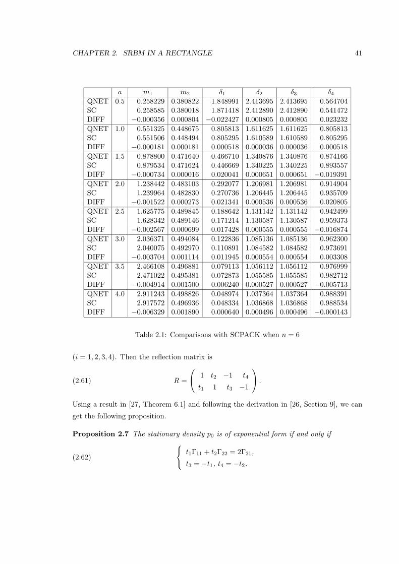
CHAPTER 2. SRBM IN A RECTANGLE 41
a m1 m2 δ1 δ2 δ3 δ4
QNET 0.5 0.258229 0.380822 1.848991 2.413695 2.413695 0.564704SC 0.258585 0.380018 1.871418 2.412890 2.412890 0.541472DIFF −0.000356 0.000804 −0.022427 0.000805 0.000805 0.023232QNET 1.0 0.551325 0.448675 0.805813 1.611625 1.611625 0.805813SC 0.551506 0.448494 0.805295 1.610589 1.610589 0.805295DIFF −0.000181 0.000181 0.000518 0.000036 0.000036 0.000518QNET 1.5 0.878800 0.471640 0.466710 1.340876 1.340876 0.874166SC 0.879534 0.471624 0.446669 1.340225 1.340225 0.893557DIFF −0.000734 0.000016 0.020041 0.000651 0.000651 −0.019391QNET 2.0 1.238442 0.483103 0.292077 1.206981 1.206981 0.914904SC 1.239964 0.482830 0.270736 1.206445 1.206445 0.935709DIFF −0.001522 0.000273 0.021341 0.000536 0.000536 0.020805QNET 2.5 1.625775 0.489845 0.188642 1.131142 1.131142 0.942499SC 1.628342 0.489146 0.171214 1.130587 1.130587 0.959373DIFF −0.002567 0.000699 0.017428 0.000555 0.000555 −0.016874QNET 3.0 2.036371 0.494084 0.122836 1.085136 1.085136 0.962300SC 2.040075 0.492970 0.110891 1.084582 1.084582 0.973691DIFF −0.003704 0.001114 0.011945 0.000554 0.000554 0.003308QNET 3.5 2.466108 0.496881 0.079113 1.056112 1.056112 0.976999SC 2.471022 0.495381 0.072873 1.055585 1.055585 0.982712DIFF −0.004914 0.001500 0.006240 0.000527 0.000527 −0.005713QNET 4.0 2.911243 0.498826 0.048974 1.037364 1.037364 0.988391SC 2.917572 0.496936 0.048334 1.036868 1.036868 0.988534DIFF −0.006329 0.001890 0.000640 0.000496 0.000496 −0.000143
Table 2.1: Comparisons with SCPACK when n = 6
(i = 1, 2, 3, 4). Then the reflection matrix is
R =
1 t2 −1 t4
t1 1 t3 −1
.(2.61)
Using a result in [27, Theorem 6.1] and following the derivation in [26, Section 9], we can
get the following proposition.
Proposition 2.7 The stationary density p0 is of exponential form if and only if t1Γ11 + t2Γ22 = 2Γ21,
t3 = −t1, t4 = −t2.(2.62)
CHAPTER 2. SRBM IN A RECTANGLE 42
In this case, the stationary density is an exponential function
x→ c·exp(λ · x),(2.63)
where
λ =
λ1
λ2
with λ1 =2(µ1 − t2µ2)(1− t1t2)Γ11
and λ2 =2(µ2 − t1µ1)(1− t1t2)Γ22
(2.64)
and c is a normalizing constant such that∫S p0(x) dx = 1.
Remark. The denominators in the expressions for λ1 and λ2 are not zero because 1− t1t2 =
(t21 Γ11 − 2t1 Γ12 + Γ22)/Γ22 > 0 by the positive definiteness of Γ.
Proof. Define two matrices
N =
1 0
0 1
-1 0
0 -1
and Q =
0 t1
t2 0
0 t3
t4 0
.
The i-th column of N ′ and the i-th column of Q′ are the unit normal and the tangential
component of vi, respectively, on Fi (i = 1, 2, 3, 4), that is,
R = N ′ +Q′.
Let U be the rotation matrix whose rows are the orthonormal eigenvectors of the covariance
matrix Γ and let A be the corresponding diagonal matrix of eigenvalues such that Γ = U ′AU ,
where U ′ = U−1. Let V = A−1/2U and define Z = V Z, X = V X and R = V R. Then X is
a (I, V µ)-Brownian motion. The i-th row of the matrix
N ≡ Λ−1/2NU ′A1/2(2.65)
is the inward unit normal to the face of the state space of Z on which Li increases, where
Λ ≡
Γ11 0 0 0
0 Γ22 0 0
0 0 Γ11 0
0 0 0 Γ22
≡ Λ1 0
0 Λ1
.
Similar to the derivation in [26, Theorem 9.23], we have R = (N ′ + Q′)Λ−1/2, where
Q′ = A−1/2U(N ′ +Q′)Λ1/2 −A1/2UN ′Λ−1/2.(2.66)
CHAPTER 2. SRBM IN A RECTANGLE 43
In a similar manner to that in the proof of Theorem 8.2 of [28], it follows from [27, 58]
that Z has an exponential form stationary distribution if and only if the following skew
symmetric condition holds
NQ′ + QN ′ = 0.(2.67)
In this case Z has a stationary distribution π such that
dπ = c exp(λ · z)dz,
where λ = 2(I − N−1Q)−1V µ and N is any nonsingular 2× 2 submatrix of N obtained by
deleting 2 rows from N and Q is the submatrix obtained by deleting the corresponding two
rows from Q. A simple algebraic manipulation gives that (2.67) is equivalent to
2NΓN ′ = N(N ′ +Q′)Λ + Λ(N +Q)N ′.(2.68)
Writing N ′ = (I,−I) and R = (R1, R2), where R1 is a 2 × 2 matrix consisting of the first
two columns of R and R2 is defined similarly, we have that the left hand side of (2.68) is
equal to 2Γ −2Γ
−2Γ 2Γ
,and the right hand side of (2.68) is equal to R1Λ1 + Λ1R
′1 R2Λ1 − Λ1R
′1
−R1Λ1 + Λ1R′2 −R2Λ1 − Λ1R
′2
.Therefore we have that (2.68) is equivalent to
2Γ = R1Λ1 + Λ1R′1(2.69)
−2Γ = R2Λ1 − Λ1R′1(2.70)
−2Γ = −R1Λ1 + Λ1R′2(2.71)
2Γ = −R2Λ1 − Λ1R′2.(2.72)
It is easy to check that (2.69) is equivalent to
t1Γ11 + t2Γ22 = 2Γ21.(2.73)
Equations (2.70) and (2.71) are redundant and they are equivalent to
t4Γ22 − t1Γ11 = −2Γ21(2.74)
t3Γ11 − t2Γ22 = −2Γ21.(2.75)
CHAPTER 2. SRBM IN A RECTANGLE 44
From equations (2.73)–(2.75), we see that they are equivalent to (2.62). Notice that (2.72),
being equivalent to t3Γ11 + t4Γ22 = −2Γ21, is satisfied when (2.62) holds.
When (2.62) holds, by taking
N1 =
1 0
0 1
, and Q1 =
0 t1
t2 0
,we can get a particular pair of N , Q by replacing N and Q in (2.65) (2.66) by N1 and Q1
respectively, i.e.,
N = Λ1/21 U ′A1/2, Q = Λ1/2
1 R′1U′A−1/2 − Λ−1/2
1 U ′A1/2.
Hence
λ = 2(I − N−1Q
)−1V µ
= 2(2I −A−1/2UΛ1R
′1U′A−1/2
)−1V µ
= 2(2I − V Λ1R
′1V′)−1
V µ
= 2(2I − V (2Γ−R1Λ1)V ′
)−1V µ
= 2(2I − 2V ΓV ′ + V R1Λ1V
′)−1V µ
= 2V ′−1Λ−11 R−1
1 µ,
where the fourth equality is obtained from (2.69). It then follows that Z has a product
form stationary distribution with density given by
z → c exp(λ · z),
where
λ = V ′λ = 2Λ−11 R−1
1 µ =(
2(µ1 − t2µ2)(1− t1t2)Γ11
,2(µ2 − t1µ1)(1− t1t2)Γ22
)′.(2.76)
This proves the proposition. 2
Let c1 and c2 satisfy
c1
∫ a
0eλ1x1dx1 = 1 and c2
∫ b
0eλ2x2dx2 = 1,
where a is the length of the rectangle and b is the height of the rectangle. Then c1c2 is the
normalizing constant for the density p0 and
m1 = c1
∫ a
0x1e
λ1x1dx1, δ1 = c1, δ3 = c1eλ1a,(2.77)
m2 = c2
∫ b
0x2e
λ2x2dx2, δ2 = c2, δ4 = c2eλ2b.(2.78)
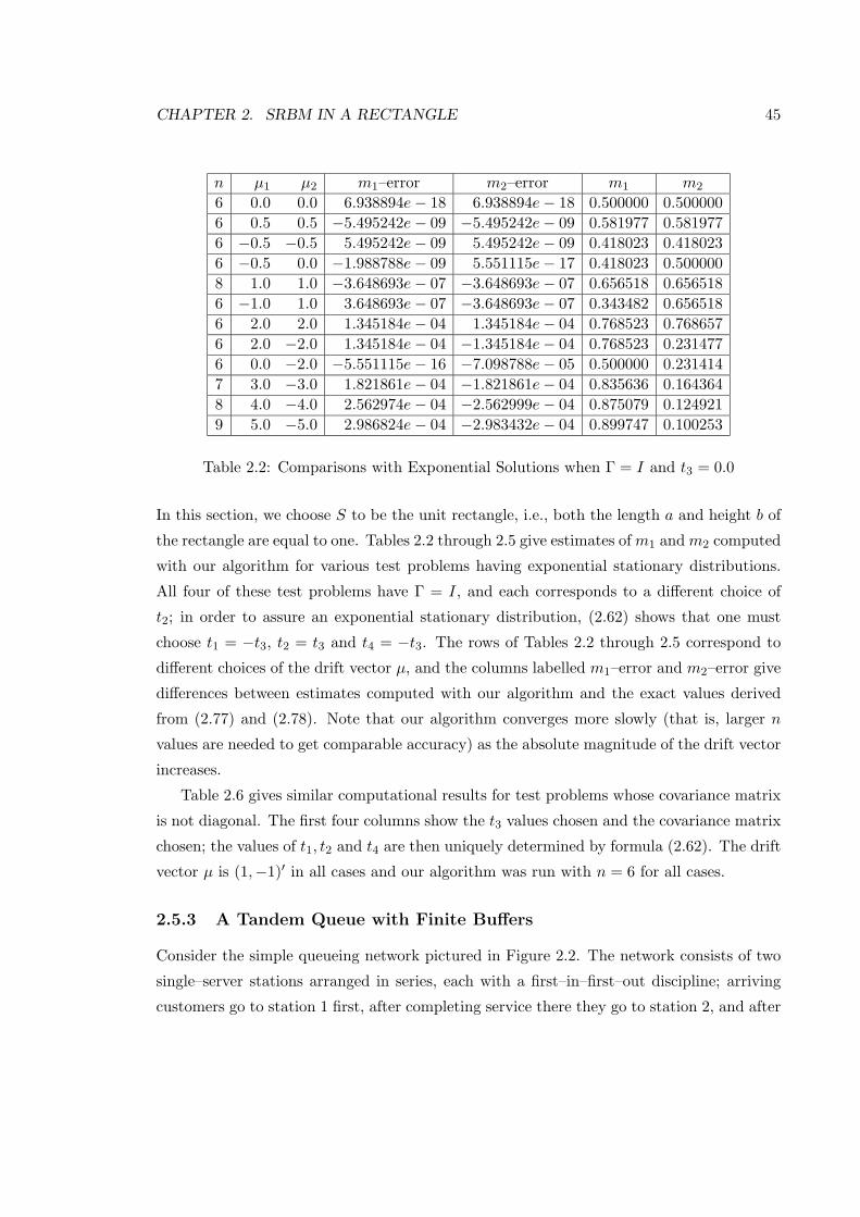
CHAPTER 2. SRBM IN A RECTANGLE 45
n µ1 µ2 m1–error m2–error m1 m2
6 0.0 0.0 6.938894e− 18 6.938894e− 18 0.500000 0.5000006 0.5 0.5 −5.495242e− 09 −5.495242e− 09 0.581977 0.5819776 −0.5 −0.5 5.495242e− 09 5.495242e− 09 0.418023 0.4180236 −0.5 0.0 −1.988788e− 09 5.551115e− 17 0.418023 0.5000008 1.0 1.0 −3.648693e− 07 −3.648693e− 07 0.656518 0.6565186 −1.0 1.0 3.648693e− 07 −3.648693e− 07 0.343482 0.6565186 2.0 2.0 1.345184e− 04 1.345184e− 04 0.768523 0.7686576 2.0 −2.0 1.345184e− 04 −1.345184e− 04 0.768523 0.2314776 0.0 −2.0 −5.551115e− 16 −7.098788e− 05 0.500000 0.2314147 3.0 −3.0 1.821861e− 04 −1.821861e− 04 0.835636 0.1643648 4.0 −4.0 2.562974e− 04 −2.562999e− 04 0.875079 0.1249219 5.0 −5.0 2.986824e− 04 −2.983432e− 04 0.899747 0.100253
Table 2.2: Comparisons with Exponential Solutions when Γ = I and t3 = 0.0
In this section, we choose S to be the unit rectangle, i.e., both the length a and height b of
the rectangle are equal to one. Tables 2.2 through 2.5 give estimates of m1 and m2 computed
with our algorithm for various test problems having exponential stationary distributions.
All four of these test problems have Γ = I, and each corresponds to a different choice of
t2; in order to assure an exponential stationary distribution, (2.62) shows that one must
choose t1 = −t3, t2 = t3 and t4 = −t3. The rows of Tables 2.2 through 2.5 correspond to
different choices of the drift vector µ, and the columns labelled m1–error and m2–error give
differences between estimates computed with our algorithm and the exact values derived
from (2.77) and (2.78). Note that our algorithm converges more slowly (that is, larger n
values are needed to get comparable accuracy) as the absolute magnitude of the drift vector
increases.
Table 2.6 gives similar computational results for test problems whose covariance matrix
is not diagonal. The first four columns show the t3 values chosen and the covariance matrix
chosen; the values of t1, t2 and t4 are then uniquely determined by formula (2.62). The drift
vector µ is (1,−1)′ in all cases and our algorithm was run with n = 6 for all cases.
2.5.3 A Tandem Queue with Finite Buffers
Consider the simple queueing network pictured in Figure 2.2. The network consists of two
single–server stations arranged in series, each with a first–in–first–out discipline; arriving
customers go to station 1 first, after completing service there they go to station 2, and after
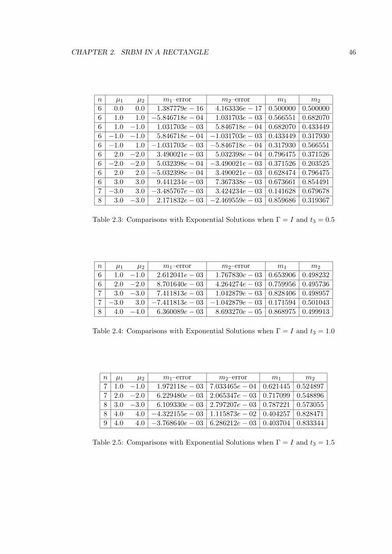
CHAPTER 2. SRBM IN A RECTANGLE 46
n µ1 µ2 m1–error m2–error m1 m2
6 0.0 0.0 1.387779e− 16 4.163336e− 17 0.500000 0.5000006 1.0 1.0 −5.846718e− 04 1.031703e− 03 0.566551 0.6820706 1.0 −1.0 1.031703e− 03 5.846718e− 04 0.682070 0.4334496 −1.0 −1.0 5.846718e− 04 −1.031703e− 03 0.433449 0.3179306 −1.0 1.0 −1.031703e− 03 −5.846718e− 04 0.317930 0.5665516 2.0 −2.0 3.490021e− 03 5.032398e− 04 0.796475 0.3715266 −2.0 −2.0 5.032398e− 04 −3.490021e− 03 0.371526 0.2035256 2.0 2.0 −5.032398e− 04 3.490021e− 03 0.628474 0.7964756 3.0 3.0 9.441234e− 03 7.367338e− 03 0.673661 0.8544917 −3.0 3.0 −3.485767e− 03 3.424234e− 03 0.141628 0.6796788 3.0 −3.0 2.171832e− 03 −2.469559e− 03 0.859686 0.319367
Table 2.3: Comparisons with Exponential Solutions when Γ = I and t3 = 0.5
n µ1 µ2 m1–error m2–error m1 m2
6 1.0 −1.0 2.612041e− 03 1.767830e− 03 0.653906 0.4982326 2.0 −2.0 8.701640e− 03 4.264274e− 03 0.759956 0.4957367 3.0 −3.0 7.411813e− 03 1.042879e− 03 0.828406 0.4989577 −3.0 3.0 −7.411813e− 03 −1.042879e− 03 0.171594 0.5010438 4.0 −4.0 6.360089e− 03 8.693270e− 05 0.868975 0.499913
Table 2.4: Comparisons with Exponential Solutions when Γ = I and t3 = 1.0
n µ1 µ2 m1–error m2–error m1 m2
7 1.0 −1.0 1.972118e− 03 7.033465e− 04 0.621445 0.5248977 2.0 −2.0 6.229480e− 03 2.065347e− 03 0.717099 0.5488968 3.0 −3.0 6.109330e− 03 2.797207e− 03 0.787221 0.5730558 4.0 4.0 −4.322155e− 03 1.115873e− 02 0.404257 0.8284719 4.0 4.0 −3.768640e− 03 6.286212e− 03 0.403704 0.833344
Table 2.5: Comparisons with Exponential Solutions when Γ = I and t3 = 1.5
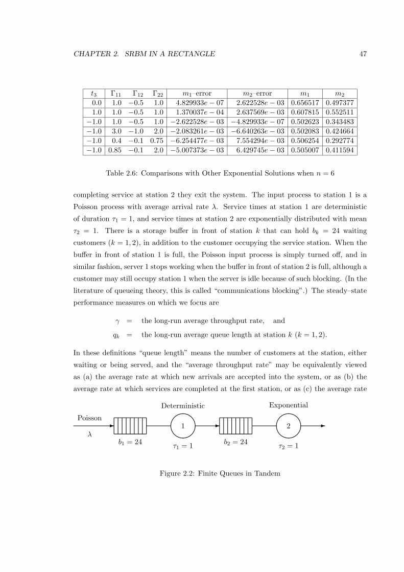
CHAPTER 2. SRBM IN A RECTANGLE 47
t3 Γ11 Γ12 Γ22 m1–error m2–error m1 m2
0.0 1.0 −0.5 1.0 4.829933e− 07 2.622528e− 03 0.656517 0.4973771.0 1.0 −0.5 1.0 1.370037e− 04 2.637569e− 03 0.607815 0.552511−1.0 1.0 −0.5 1.0 −2.622528e− 03 −4.829933e− 07 0.502623 0.343483−1.0 3.0 −1.0 2.0 −2.083261e− 03 −6.640263e− 03 0.502083 0.424664−1.0 0.4 −0.1 0.75 −6.254477e− 03 7.554294e− 03 0.506254 0.292774−1.0 0.85 −0.1 2.0 −5.007373e− 03 6.429745e− 03 0.505007 0.411594
Table 2.6: Comparisons with Other Exponential Solutions when n = 6
completing service at station 2 they exit the system. The input process to station 1 is a
Poisson process with average arrival rate λ. Service times at station 1 are deterministic
of duration τ1 = 1, and service times at station 2 are exponentially distributed with mean
τ2 = 1. There is a storage buffer in front of station k that can hold bk = 24 waiting
customers (k = 1, 2), in addition to the customer occupying the service station. When the
buffer in front of station 1 is full, the Poisson input process is simply turned off, and in
similar fashion, server 1 stops working when the buffer in front of station 2 is full, although a
customer may still occupy station 1 when the server is idle because of such blocking. (In the
literature of queueing theory, this is called “communications blocking”.) The steady–state
performance measures on which we focus are
γ = the long-run average throughput rate, and
qk = the long-run average queue length at station k (k = 1, 2).
In these definitions “queue length” means the number of customers at the station, either
waiting or being served, and the “average throughput rate” may be equivalently viewed
as (a) the average rate at which new arrivals are accepted into the system, or as (b) the
average rate at which services are completed at the first station, or as (c) the average rate
Poisson-
λb1 = 24
Deterministic
"!#
1
τ1 = 1
-
b2 = 24
Exponential
"!#
2
τ2 = 1
-
Figure 2.2: Finite Queues in Tandem
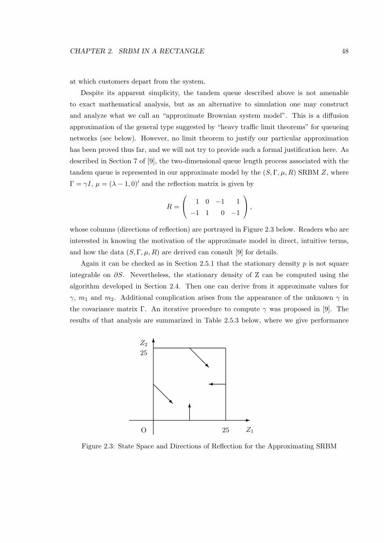
CHAPTER 2. SRBM IN A RECTANGLE 48
at which customers depart from the system.
Despite its apparent simplicity, the tandem queue described above is not amenable
to exact mathematical analysis, but as an alternative to simulation one may construct
and analyze what we call an “approximate Brownian system model”. This is a diffusion
approximation of the general type suggested by “heavy traffic limit theorems” for queueing
networks (see below). However, no limit theorem to justify our particular approximation
has been proved thus far, and we will not try to provide such a formal justification here. As
described in Section 7 of [9], the two-dimensional queue length process associated with the
tandem queue is represented in our approximate model by the (S,Γ, µ,R) SRBM Z, where
Γ = γI, µ = (λ− 1, 0)′ and the reflection matrix is given by
R =
1 0 −1 1
−1 1 0 −1
,whose columns (directions of reflection) are portrayed in Figure 2.3 below. Readers who are
interested in knowing the motivation of the approximate model in direct, intuitive terms,
and how the data (S,Γ, µ,R) are derived can consult [9] for details.
Again it can be checked as in Section 2.5.1 that the stationary density p is not square
integrable on ∂S. Nevertheless, the stationary density of Z can be computed using the
algorithm developed in Section 2.4. Then one can derive from it approximate values for
γ, m1 and m2. Additional complication arises from the appearance of the unknown γ in
the covariance matrix Γ. An iterative procedure to compute γ was proposed in [9]. The
results of that analysis are summarized in Table 2.5.3 below, where we give performance
-
6
O Z1
Z2
25
25
@@@R
6
@@@R
Figure 2.3: State Space and Directions of Reflection for the Approximating SRBM
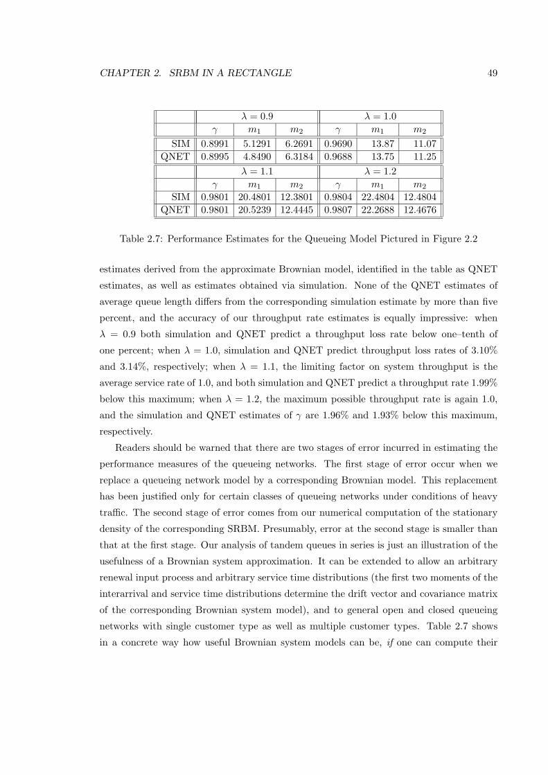
CHAPTER 2. SRBM IN A RECTANGLE 49
λ = 0.9 λ = 1.0γ m1 m2 γ m1 m2
SIM 0.8991 5.1291 6.2691 0.9690 13.87 11.07QNET 0.8995 4.8490 6.3184 0.9688 13.75 11.25
λ = 1.1 λ = 1.2γ m1 m2 γ m1 m2
SIM 0.9801 20.4801 12.3801 0.9804 22.4804 12.4804QNET 0.9801 20.5239 12.4445 0.9807 22.2688 12.4676
Table 2.7: Performance Estimates for the Queueing Model Pictured in Figure 2.2
estimates derived from the approximate Brownian model, identified in the table as QNET
estimates, as well as estimates obtained via simulation. None of the QNET estimates of
average queue length differs from the corresponding simulation estimate by more than five
percent, and the accuracy of our throughput rate estimates is equally impressive: when
λ = 0.9 both simulation and QNET predict a throughput loss rate below one–tenth of
one percent; when λ = 1.0, simulation and QNET predict throughput loss rates of 3.10%
and 3.14%, respectively; when λ = 1.1, the limiting factor on system throughput is the
average service rate of 1.0, and both simulation and QNET predict a throughput rate 1.99%
below this maximum; when λ = 1.2, the maximum possible throughput rate is again 1.0,
and the simulation and QNET estimates of γ are 1.96% and 1.93% below this maximum,
respectively.
Readers should be warned that there are two stages of error incurred in estimating the
performance measures of the queueing networks. The first stage of error occur when we
replace a queueing network model by a corresponding Brownian model. This replacement
has been justified only for certain classes of queueing networks under conditions of heavy
traffic. The second stage of error comes from our numerical computation of the stationary
density of the corresponding SRBM. Presumably, error at the second stage is smaller than
that at the first stage. Our analysis of tandem queues in series is just an illustration of the
usefulness of a Brownian system approximation. It can be extended to allow an arbitrary
renewal input process and arbitrary service time distributions (the first two moments of the
interarrival and service time distributions determine the drift vector and covariance matrix
of the corresponding Brownian system model), and to general open and closed queueing
networks with single customer type as well as multiple customer types. Table 2.7 shows
in a concrete way how useful Brownian system models can be, if one can compute their
CHAPTER 2. SRBM IN A RECTANGLE 50
stationary distributions.
2.6 Concluding Remarks
Let us return to the setting of Section 2.4, where the problem of computing the stationary
density p was cast as a least squares problem. The treatment given there can be generalized
in the following way, which may be important for both practical and theoretical purposes.
(In this section the letter q will be re–used with a new meaning, but that should cause no
confusion.) Let q0 be a strictly positive function on the interior S of the rectangle S, and
let q1, . . . , q4 be strictly positive functions on the boundary surfaces F1, . . . , F4 respectively.
Defining
q(x) = (q0; q1, q2, q3, q4).(2.79)
we call q a “reference density” and we define a corresponding “reference measure” η via
η(dx) ≡ qdλ = (q0 dx; q1 dσ1, . . . , q4 dσ4).(2.80)
If we work in the Hilbert space L2(S, η) rather than the space L2(S, dλ) used in Section 2.4,
then the focus is on the unknown function r defined by
r(x) ≡ p/q = (p0/q0; p1/q1, · · · , p4/q4).(2.81)
That is, with the inner product defined by (f, g) =∫S(f ·g) dη, our basic adjoint relationship
(2.35) says that Af ⊥ r for all f ∈ C2(S), and hence one may proceed exactly as in
Sections 2.4 to devise an algorithm for approximate computation of r by projection in
L2(S, η). Of course, the final estimate of r is converted to an estimate of p via p = rq,
where q is the reference density chosen.
A different computational procedure is obtained depending on how one chooses the
reference density q and the functions f1, f2, . . . that are used to build up the approximating
subspaces H1,H2, . . . via Hn = spanAf1, . . . ,Afn. Recall that in Section 2.4 we took
f1, f2, . . . to be polynomial functions, but other choices are obviously possible. One wants to
choose q and f1, f2, . . . in such a way that the inner products (Afm,Afn) can be determined
analytically, and in such a way as to accelerate convergence of the algorithm. From a
theoretical standpoint, the freedom to choose q is important because one may have r ∈L2(S, η) even though p 6∈ L2(S, dλ) (e.g. by choosing q = p, we have r = 1 ∈ L2(S, η)),
and thus a judicious choice of reference density enables a rigorous proof of convergence in

CHAPTER 2. SRBM IN A RECTANGLE 51
L2(S, η). From a practical standpoint, one may be able to choose q in such a way that
convergence is accelerated, taking q to be a “best guess” of the unknown density p based on
either theory or prior computations. In Chapter 4, we will discuss computation of stationary
distributions on unbounded regions, where a proper choice of reference density is essential
to efficient computation.
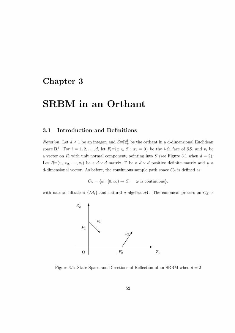
Chapter 3
SRBM in an Orthant
3.1 Introduction and Definitions
Notation. Let d ≥ 1 be an integer, and S≡Rd+ be the orthant in a d-dimensional Euclidean
space Rd. For i = 1, 2, . . . , d, let Fi≡x ∈ S : xi = 0 be the i-th face of ∂S, and vi be
a vector on Fi with unit normal component, pointing into S (see Figure 3.1 when d = 2).
Let R≡(v1, v2, . . . , vd) be a d × d matrix, Γ be a d × d positive definite matrix and µ a
d-dimensional vector. As before, the continuous sample path space CS is defined as
CS = ω : [0,∞)→ S, ω is continuous,
with natural filtration Mt and natural σ-algebra M. The canonical process on CS is
-
6
O Z1
Z2
@@@R
v1
F1
v2
F2
Figure 3.1: State Space and Directions of Reflection of an SRBM when d = 2
52
CHAPTER 3. SRBM IN AN ORTHANT 53
denoted by Z = Z(t, ω), t ≥ 0 defined by
Z(t, ω) = ω(t).
The symbol ω is often suppressed in Z. The SRBM in an orthant S is defined as follows.
Definition 3.1 Z is said to be a semimartingale reflected Brownian motion (abbreviated as
SRBM) associated with data (S,Γ, µ,R) if there is a family of probability measures Px, x ∈S defined on the filtered probability space (CS ,M, Mt) such that for each x ∈ S we
have
(3.1) Z(t) = X(t) +RL(t) = X(t) +∑di=1 Li(t) · vi ∀t ≥ 0, Px-a.s.,
(3.2) X(0) = x, Px-a.s. and X is a d-dimensional Brownian motion with covariance matrix
Γ and drift vector µ such that X(t)− µt,Mt, t ≥ 0 is a martingale under Px,
(3.3) L is a continuous Mt-adapted d-dimensional process such that L(0) = 0 Px-a.s, L
is non-decreasing, and Li increases only at times t when Zi(t) = 0, i = 1, . . . , d.
Remark. This is the definition of SRBM used by Reiman and Williams [41]. It was pointed
out by those authors that X(t)−µt being an Mt-martingale is necessary for an SRBM
to have certain desired properties.
The SRBM Z defined above behaves like a d-dimensional Brownian motion with drift
vector µ and covariance matrix Γ in the interior of its state space. When the boundary
face Fi is hit, the process Li (sometimes called the local time of Z on Fi) increases, causing
an instantaneous displacement of Z in the direction given by vi; the magnitude of the
displacement is the minimal amount required to keep Z always inside S. Therefore, we
call Γ, µ and R the covariance matrix, the drift vector and the reflection matrix of Z,
respectively.
Definition 3.2 The SRBM is said to be unique if the family Px, x ∈ S is unique.
Definition 3.3 The matrix R is said to be Minkowski if I −R ≥ 0 and I −R is transient,
that is, all the eigenvalues of I −R are less than one, where I is the d× d identity matrix.
Definition 3.4 A d× d matrix A is said to be an S matrix if there exists a d-dimensional
vector u ≥ 0 such that Au > 0, and to be a completely-S matrix if each of its principal
submatrices is an S matrix.
CHAPTER 3. SRBM IN AN ORTHANT 54
Harrison and Reiman [25], by using a unique path-to-path mapping, defined an SRBM in
S when the reflection matrix R is Minkowski. This class of SRBM’s arise naturally from
queueing networks with homogeneous customers. It is known [24] that the reflection matrix
R of an SRBM which arises from a queueing network with heterogeneous customers is, in
general, not Minkowski. Reiman and Williams [41] proved that R being completely-S is a
necessary condition for the existence of an SRBM in S.
Recently Taylor and Williams [50], by considering solutions of local submartingale prob-
lems, proved the existence and uniqueness of an SRBM when R is a completely-S matrix.
We state their result in the following proposition.
Proposition 3.1 Assume R is a completely-S matrix. For any positive definite matrix Γ
and vector µ, there exists a unique family of probability measures Px, x ∈ S on the filtered
space (CS ,M, Mt) such that Z together with Px, x ∈ S is an (S,Γ, µ,R)-SRBM.
In this chapter, Ex will denote the expectation operator with respect to the probability
measure Px, and for a probability measure π on S, define
Pπ(·) ≡∫SPx(·)π(dx);
then Eπ denotes the corresponding expectation.
Readers should keep in mind that there are RBM’s which are not SRBM’s, see Harrison,
Landau and Shepp [23] and Varadhan and Williams [53]. However, in this dissertation we
only consider the class of RBM’s which have the semimartingale representation (3.1) as
defined in Definition 3.1 above.
In this chapter we first prove the Feller continuity of an SRBM, and therefore prove
that an SRBM is a strong Markov process. It is reported that Taylor and Williams [50]
give a different proof of the Feller continuity of an SRBM. Then we give an alternative
characterization of an SRBM via a solution to a constrained martingale problem. This
alternative characterization is critical in proving sufficiency of a basic adjoint relationship
governing the stationary distribution of an SRBM, which was conjectured by Harrison and
Williams [26] when R is Minkowski.
3.2 Feller Continuity and Strong Markov Property
Definition 3.5 The Z with Px, x ∈ S is said to be Feller continuous if for any f ∈ Cb(S),
Ttf ∈ Cb(S) for each t ≥ 0. Here Ttf(x) ≡ Exf(Z(t)).
CHAPTER 3. SRBM IN AN ORTHANT 55
Theorem 3.1 Let Z with Px, x ∈ S be an SRBM. Suppose xn is a sequence in S which
converges to x ∈ S. Then Pxn converges weakly to Px.
Proof. In this proof only, we need a bigger probability space. Let C+Rd
denote the space
of continuous functions x(·) : [0,∞) → Rd with x(0) ≥ 0 and Λd denote the space of
continuous functions l(·) : [0,∞) → Rd+ such that l(0) = 0 and each component of l(·) is
a non-decreasing function. Both CRd+and Λd are endowed with the Skorohod topology.
For z(·) ∈ CS , x(·) ∈ C+Rd
and l(·) ∈ Λd, define ω(t) = (z(t), x(t), l(t)) for each t ≥ 0.
Then ω is a generic element of ΩS ≡ CS × C+Rd× Λd. Define three canonical processes
Z,X and L via Z(t, ω) = z(t), X(t, ω) = x(t) and L(t, ω) = l(t), and filtration M0t via
M0t ≡ σZ(s), X(s), L(s) : 0 ≤ s ≤ t, t ≥ 0. It is obvious that the family Px, x ∈ S on
CS induces a family of probability measures Qx, x ∈ S on the sample space (ΩS , M0t ),
such that, for each x ∈ S, the following holds.
(3.4) For each t ≥ 0, Z(t) = X(t) +RL(t), Qx-a.s.
(3.5) Under Qx, X is a (Γ, µ)-Brownian motion starting from x and X(t)−µt is a M0t -
martingale.
(3.6) Li increases only when at times Z(·) ∈ Fi almost surely in Qx, i.e.,∫ ∞0
Zi(t) dLi(t) = 0, Qx-a.s. (i = 1, 2, . . . , d).
Let xn be a sequence in S such that xn → x, obviously QxnX−1 ⇒ QxX
−1, therefore
QxnX−1 is tight. Hence for any ε > 0, there exists a compact set A ⊂ C+Rd
such that
QxnX−1(A) > 1− ε, for all n.
Let A ⊂ ΩS be defined as ω = (z, x, l) ∈ A if and only if x ∈ A and
z = x+Rl,
∫ ∞0
z(t) dl(t) = 0,(3.7)
where ∫ t
0z(s) dl(s) ≡
(∫ t
0z1(s) dl1(s), . . . ,
∫ t
0zd(s) dld(s)
)′, t ≥ 0.
It follows from Proposition 1 of [2] that A is precompact. Because
Qxn(A) = QxnX−1(A) > 1− ε,
CHAPTER 3. SRBM IN AN ORTHANT 56
we have proved that the family Qxn is tight, and Prohorov’s Theorem, see [3, Theorem 6.1
of Chapter 1], asserts that Qxn is weakly relatively compact. Let Q∗ be any accumulation
point of Qxn. There is a subsequence of Qxn that converges to Q∗ weakly. For notational
convenience, we assume the sequence itself converges, that is, Qxn ⇒ Q∗. We are going to
prove that Z is an SRBM starting from x under Q∗, i.e.,
Q∗Z−1 = Px,(3.8)
Then it follows from (3.8) that
Pxn = QxnZ−1 ⇒ Q∗Z
−1 = Px.
To prove (3.8), we prove that (3.4) through (3.6) hold under Q∗. It is clear that under Q∗,
X is a (Γ, µ)-Brownian motion starting from x. If X(t) were bounded for each t, because
X(t)− µt is a M0t -martingale under each Qxn and Qxn ⇒ Q∗, X(t)− µt is a M0
t -martingale under each Q∗. A general argument can be obtained through standard localizing
arguments. Therefore (3.5) holds under Q∗. To show that (3.4) and (3.6) hold under Q∗,
define two functions ΩS → CRd as
f1(ω)(t) ≡ z(t)− x(t)− l(t), t ≥ 0,
f2(ω)(t) ≡∫ t
0z(s) dl(s), t ≥ 0.(3.9)
It is obvious that f1 is continuous and it follows from the following Lemma 3.1 that f2 is
continuous. Hence Ai ≡ ω : fi(ω) = 0 is a closed set in ΩS (i = 1, 2). Because (3.4) and
(3.6) hold under Qxn , Qxn(Ai) = 1 for each n (i = 1, 2). Therefore, see [3, Theorem 2.1 of
Chapter 1],
1 = lim supn→∞
Qxn(Ai) ≤ Q∗(Ai), (i = 1, 2).
Thus Q∗(Ai) = 1 (i = 1, 2), which implies that (3.4) and (3.6) hold under Q∗. Therefore we
have proved Z under Q∗ is an SRBM starting from x, and by the uniqueness of the SRBM,
Px = Q∗Z−1. This proves (3.8) and thus proves the theorem. 2
Lemma 3.1 The function f2 : ΩS → CRd defined in (3.9) is continuous.
Proof. Let zn ∈ CS be a sequence converging to z ∈ CS and ln ∈ Λd be a sequence
converging to l ∈ Λd. Fix a T > 0, we like to show
sup0≤t≤T
∣∣∣∣∫ t
0zn(s) dln(s)−
∫ t
0z(s) dl(s)
∣∣∣∣→ 0,
CHAPTER 3. SRBM IN AN ORTHANT 57
as n→∞. To see this, for each positive integer k, define a step function z(k) as
z(k)(t) ≡ z (iT/k) , ifi
kT ≤ t < i+ 1
kT.
It is clear that sup0≤t<T |z(k)(t)− z(t)| → 0 as k →∞, and
sup0≤t≤T
∣∣∣∣∫ t
0zn(s) dln(s)−
∫ t
0z(s) dl(s)
∣∣∣∣≤ sup
0≤t≤T
∫ t
0|zn(s)− z(s)| dln(s) + sup
0≤t≤T
∣∣∣∣∫ t
0z(s) d (ln(s)− l(s))
∣∣∣∣≤ sup
0≤s≤T|zn(s)− z(s)|ln(T ) +
∫ T
0|z(s)− z(k)(s)|d (ln(s) + l(s))
+ sup0≤t≤T
∣∣∣∣∫ t
0z(k)(s) d(ln(s)− l(s))
∣∣∣∣≤ sup
0≤s≤T|zn(s)− z(s)|ln(T ) + sup
0≤s<T|z(s)− z(k)(s)|(ln(T ) + l(T ))
+k∑i=1
z (iT/k) |(ln ((i+ 1)T/k)− l ((i+ 1)T/k))− (ln (iT/k)− l (iT/k))| .
Since ln(T ) is bounded in n, for any ε > 0, choose k big enough so that the middle term
in the previous expression is less than ε/2, then for n large enough we have the first term
adding the third term is less than ε/2. This proves our lemma. 2
Corollary 3.1 Z with Px, x ∈ S is Feller continuous, i.e., for any f ∈ Cb(S) and any
t ≥ 0, x→ Ex [f(Z(t))] is continuous.
Proof. Obviously, for any f ∈ Cb(S), g : CS → R defined by g(z(·)) ≡ f(z(t)) is a bounded
continuous function on CS , hence, from Theorem 3.1 and the definition of weak convergence,
Ttf(x) ≡ Ex [f(Z(t))] = Ex [g(Z(·))] is a continuous function of x. 2
It is now easy to show that the probability family associated with an SRBM Z is Borel
measurable, i.e., for any A ∈ M, x→ Px(A) is a Borel measurable function on S. In fact,
we are going to show
Corollary 3.2 Suppose h : CS → R is bounded and M-measurable. Then the function
x→ Ex [h(Z(·))] , ∀x ∈ S
is a Borel measurable function on S.
CHAPTER 3. SRBM IN AN ORTHANT 58
Proof. The corollary can be obtained from Theorem 3.1 directly. 2
Now we have the following theorem, which ensures that an SRBM is a strong Markov
process.
Theorem 3.2 An SRBM Z together with a measurable family Px,∈ S on a filtered space
(Ω,F , Ft) is a strong Markov process, i.e., for each x ∈ S,
Ex [f(Z(τ + t))|Fτ ] = T (t)f(Z(τ)), Px-a.s.
for all f ∈ B(S), t ≥ 0, and Px-a.s. finite Ft-stopping time τ .
Proof. Since the SRBM Z with the family Px, x ∈ S is unique and Feller continuous, it
follows from the proof of Theorem 4.2 in Chapter 4 of [11] that Z together with Px, x ∈ Sis strong Markov. 2
3.3 Constrained Martingale Problem
Using the ideas of Kurtz [32, 31], we now characterize an SRBM as a solution of a corre-
sponding constrained martingale problem. This alternative characterization of an SRBM
plays a key role in proving the sufficiency of a basic adjoint relationship for the stationary
distribution in Section 3.5. For f ∈ C2(S), define
Gf≡12
d∑i=1
d∑j=1
Γij∂2f
∂xi∂xj+
d∑i=1
µi∂f
∂xi,(3.10)
Dif(x)≡vi · ∇f(x) for x ∈ Fi (i = 1, 2, . . . , d).(3.11)
The operatorsG andDi defined in (3.10) and (3.11), respectively, can be viewed as mappings
from C2K(Rd) → CK(Rd). Denote D ≡ (D1, . . . , Dd). From now on, C2
K(Rd) will be taken
implicitly as the domain of (G,D). In the following, P(S) denotes the set of probability
measures on S.
Definition 3.6 For any π ∈ P(S), by a local time solution of the constrained martingale
problem for (S,G,D;π) we mean a pair of d-dimensional continuous processes (Z,L) on
some filtered probability space (Ω, Ft,F , P ) such that
(3.12) Z(t) ∈ S for all t ≥ 0 and PZ(0)−1 = π.
CHAPTER 3. SRBM IN AN ORTHANT 59
(3.13) f(Z(t))−∫ t
0 Gf(Z(s)) ds−∑di=1
∫ t0 Dif(Z(s)) dLi(s)
is a Ft-martingale under P .
(3.14) P -almost surely, Li(0) = 0, Li(·) non-decrease, and Li(·) increases only at times t
when Z(t) ∈ Fi (i = 1, . . . , d).
The following theorem gives the equivalence of an SRBM to a local time solution of the
corresponding constrained martingale problem.
Theorem 3.3 For π ∈ P(S), suppose Z together with Px, x ∈ S on (CS , Mt,M) is
an SRBM and L is the associated local time defined in (3.3). Then, under Pπ, (Z,L) on
(CS , Mt,M) is a solution of the constrained martingale problem for (S,G,D;π). Con-
versely, suppose (Z,L) on a filtered probability space (Ω, Ft,F , P ) is a local time solution
of the constrained martingale problem for (S,G,D;π). Then Z is an SRBM starting with
π, i.e.,
(a) Z(t) = X(t) +RL(t) = X(t) +∑di=1 Li(t) · vi ∈ S ∀t ≥ 0, P -a.s., where
(b) PX(0)−1 = π and X is a d-dimensional Brownian motion with covariance matrix Γ
and drift vector µ such that X(t)− µt,Ft, t ≥ 0 is a martingale under P , and
(c) L is a continuous Ft-adapted d-dimensional process such that P -a.s. L(0) = 0, L is
non-decreasing, and Li increases only at times t when Zi(t) = 0, i = 1, . . . , d.
Proof. Suppose that Z together Px, x ∈ S on (CS , Mt,M) is an SRBM, associated
with X and L as in (3.2) and (3.3). Then, Z(t) ∈ S, and under Pπ, it is obvious that
Z(0) = X(0) has the distribution π. For f ∈ C2b (S), by Ito’s formula, it is clear that
(3.13) is a Mt-martingale. The conditions on L in (c) is equivalent to the condition in
(3.14). Therefore, (Z,L) is a local time solution of the constrained martingale problem for
(G,D;π).
Conversely, suppose (Z,L) on a filtered probability space (Ω, Ft,F , P ) is a local time
solution of the constrained martingale problem for (G,D;π). Define
ξ(t) ≡ Z(t)− Z(0)−RL(t)− µt = Z(t)− Z(0)−d∑i=1
viLi(t)− µt,
we first show that ξ is a Ft-Brownian motion with covariance matrix Γ and zero drift.
For each integer n > 0, let
σn = inft ≥ 0 : |ξ(t)| > n.
CHAPTER 3. SRBM IN AN ORTHANT 60
Then σn is a stopping time. Taking an f ∈ C2K(Rd) such that f(x) = xi on x : |x| ≤ n,
since (3.13) is a martingale for the f , by the optional sampling theorem,
f(Z(t ∧ σn))−∫ t∧σn
0Gf(Z(s)) ds−
d∑i=1
∫ t∧σn
0Dif(X(s)) dLi(s)(3.15)
is a continuous Ft-martingale. Because f(x) = xi, Gf(x) = µi, and Djf(x) = vij for
|x| ≤ n, we see from (3.15) that ξi(t ∧ σn) is a martingale, i = 1, . . . , d. Since σn ↑ ∞ as
n → ∞, ξi is a continuous local martingale. Similarly, by choosing f ∈ C2K(Rd) such that
f(x) = xixj for x ∈ x : |x| ≤ n, (3.13) gives that
Zi(t ∧ σn)Zj(t ∧ σn) − Γij(t ∧ σn)−∫ t∧σn
0(µiZj(s) + µjZi(s)) ds(3.16)
−d∑
k=1
∫ t∧σn
0
(vikZj + vikZi
)dLk(s)
is a martingale. On the other hand, by Ito’s formula, we have
Zi(t ∧ σn)Zj(t ∧ σn) = Zi(0)Zj(0) +∫ t∧σn
0Zi dξj(s) +
∫ t∧σn
0Zj(s) dξi(s)(3.17)
+∫ t∧σn
0(µiZj(s) + µjZi(s)) ds+ 〈ξi, ξj〉(t ∧ σn)
+d∑
k=1
∫ t∧σn
0
(vikZj + vikZi
)dLk(s),
where 〈ξi, ξj〉(t) is the quadratic variational process of ξi and ξj . The first two stochastic
integrals on the right hand side of (3.17) are martingales. From this and from (3.16) and
(3.17), we have
〈ξi, ξj〉(t ∧ σn)− Γij(t ∧ σn)
is a martingale. Therefore, we have the quadratic variational process of ξi and ξj
〈ξi, ξj〉(t) = Γijt.
By Theorem 7.1 of [29, Chapter 2], we can find a d-dimensional standard Ft−Brownian
motion B = (B(t)) on the same probability space (Ω,F , P ) such that
ξi(t) =d∑
k=1
(Γ12 )ikBk(t), i = 1, · · · , d,
where Γ12 is the square root of the positive definite covariance matrix Γ. Therefore, ξ is a
d-dimensional Brownian motion starting from zero with covariance matrix Γ and drift zero.
CHAPTER 3. SRBM IN AN ORTHANT 61
By letting X(t) ≡ Z(0) + ξ(t) + µt, then X is a Brownian motion with initial distribution
PX(0)−1 = π, covariance matrix Γ, and drift vector µ. Clearly, under P , (Z,X,L) satisfies
the equations (3.1) to (3.3) with X(0) = x replaced by PX(0)−1 = π in (3.2). This proves
our theorem. 2
3.4 Existence of a Stationary Distribution
From Theorem 3.2, an SRBM Z is a strong Markov process. We ask when its stationary
distribution exists, and if there is one, how to characterize such a stationary distribution.
Definition 3.7 A probability measure π on S is called a stationary distribution of the
SRBM Z if for every bounded Borel function f on S and every t > 0∫STtf(x)π(dx) =
∫Sf(x)π(dx),
where Tt, t ≥ 0 is the semigroup as defined in Definition 3.5 associated with the strong
Markov process Z.
In this section, we first establish a criterion for the existence of a stationary distribution
via Liapunov functions. Then we show when R−1 ≥ 0 and R is symmetric, Z has a
stationary distribution if and only if R−1µ < 0. This case was not covered by Harrison and
Williams [26], who considered only the case of a Minkowski reflection matrix.
3.4.1 Necessary Conditions
Let σi denote (d− 1)-dimensional Lebesgue measure (surface measure) on the face Fi. The
following proposition was proved in [26] when the reflection matrix R is Minkowski, and the
proof can be generalized to the case when R is completely-S by using the following lemma.
Lemma 3.2 Suppose that Z is an SRBM with local time L as in (3.3). Then for each
t ≥ 0,
supx∈S
ExLi(t) <∞.
Proof. R is a completely-S matrix, hence it is completely saillante. Therefore, the lemma
is an immediate consequence of Lemma 1 in [2]. 2
Proposition 3.2 Any stationary distribution for an SRBM Z is unique. If π is the sta-
tionary distribution,
CHAPTER 3. SRBM IN AN ORTHANT 62
(a) π is equivalent to Lebesgue measure on S, and for each x ∈ S and each f ∈ Cb(S),
limn→∞
1n
n∑i=1
Ex [f(Z(i))] =∫Sf(z) dπ(z);
(b) there is a finite Borel measure νi on Fi such that νi ≈ σi and for each bounded Borel
function f on Fi and t ≥ 0,
Eπ
[∫ t
0f(Z(s)) dLi(s)
]= t
∫Fi
f dνi, (i = 1, 2, . . . , d).
Proof. The proof of part (a) is essentially the same as the proof of Theorem 7.1 of [26],
and with Lemma 3.2 replacing Lemma 8.4 in [26], the proof of part (b) can also be readily
carried over from that of Theorem 8.1 of [26]. 2
In terms of the primitive data (Γ, µ,R) of an SRBM, we have the following necessary
conditions.
Theorem 3.4 If Z has a stationary distribution, then
(a) the reflection matrix R is invertible, and
(b) R−1µ < 0 if R−1 ≥ 0.
Proof. Suppose that π is a stationary distribution of an SRBM Z. (a) Assume R is singular.
Then there exists a non-trivial vector v such that v′R = 0, where “prime” is the transpose
operator. For the SRBM Z, we have the semimartingale representation (3.1). Therefore
v′Z(t) = v′X(t) + v′RL(t) = v′X(t),(3.18)
since v′R = 0. From Proposition 3.2 (a), Z is ergodic, and hence v′Z is ergodic. On
the other hand, v′X is a one-dimensional (v′Γv, v′µ)-Brownian motion, which can not be
ergodic, contradicting to (3.18). Thus, R can not be singular, this proves part (a).
(b) From part (a), R is invertible and from representation (3.1),
Z∗(t) ≡ R−1Z(t) = R−1X(t) + L(t), t ≥ 0.
Since R−1 ≥ 0, we have Z∗(t) ≥ 0. The rest of arguments can follow from the proof of
Lemma 6.14 in [26]. 2
CHAPTER 3. SRBM IN AN ORTHANT 63
3.4.2 A Sufficient Condition
When R is Minkowski, Harrison and Williams [26] proved that Z has a stationary distri-
bution if and only if R−1µ < 0. Their proof relied heavily on the fact that R is Minkowski,
in which case the SRBM Z has an alternative characterization as in the Appendix of [39].
By using the alternative characterization, they were able to show a transformed process of
Z is stochastically monotone, and thus proved the above assertion. In the following, for a
general completely-S reflection matrix R with R−1 ≥ 0, we establish a sufficient condition
for the existence of a stationary distribution via existence of a Liapunov function. If R is
further assumed to be symmetric, we are able to construct such a Liapunov function when
R−1µ < 0; thus Z has a stationary distribution in this case.
Let C0(S) be the set of f ∈ Cb(S) such that limx→∞ f(x) = 0, i.e., for any ε > 0, there
exists an R > 0 such that for all x ∈ |x| > R ∩ S, |f(x)| < ε.
Definition 3.8 An SRBM Z is said to be C0(S)-Feller if for every f ∈ C0(S), Ttf(x) ≡Exf(Z(t)) ∈ C0(S) for each t ≥ 0.
Remark. Let P (t, x, ·) ∈ P(S), t ≥ 0, x ∈ S be the transition probabilities of Z, that
is, for each A ∈ BS , (t, x) → P (t, x,A) is a Borel measurable function and Ttf(x) =∫S f(y)P (t, x, dy) for each f ∈ B(S). Since Z is Feller, it can be checked [8] that Z is
C0(S)-Feller if and only if for any compact subset K ⊂ S,
limx→∞
P (t, x,K) = 0.(3.19)
A Markov process Z = Z(t), t ≥ 0 taking values in S is said to be stochastically
continuous if for every f ∈ Cb(S), t → Exf(Z(t)) is a continuous function for each x ∈ S.
The following proposition, tailored to the present setting, was proved in [8] for a Markov
process taking values in any complete separable metric state space.
Proposition 3.3 If Z is stochastically continuous, C0(S)-Feller Markov process valued in
S, then the following two statements are equivalent.
(a) For any x ∈ S and any compact subset K ⊂ S,
limT→∞
1T
∫ T
0P (t, x,K) dt = 0;
(b) There exists no stationary distribution for the Markov process Z. 2
CHAPTER 3. SRBM IN AN ORTHANT 64
Lemma 3.3 If R−1 ≥ 0, then any SRBM Z with reflection matrix R is C0(S)-Feller.
Proof. From representation (3.1), we have
Z∗ ≡ R−1Z = R−1X + L.
For any given r > 0, let
f(x) =r2
r2 + |x|2, x ∈ Rd,
then f ∈ C2 and we have
∂f
∂xi(x) = −2xi
r2f2(x),(3.20)
∂2f
∂xi∂xj(x) =
8xixjr4
f3(x)− 2δijr2
f2(x),(3.21)
where δij = 0 if i 6= j and δij = 1 otherwise. Hence f ∈ C2b (Rd). For each x ∈ S, applying
Ito’s formula with f on the completion (CS ,M, Px) of (CS ,M, Px), we obtain Px-a.s. for
all t ≥ 0
f(Z∗(t)) = f(Z∗(0)) +∫ t
0G∗f(Z∗(s))ds+
d∑i=1
∫ t
0
∂f
∂xi(Z∗(s)) dξi(s)(3.22)
+d∑i=1
∫ t
0
∂f
∂xi(Z∗(s)) dLi(s),
where G∗f is a second order elliptic operator associated with covariance matrix R−1ΓR′−1
and drift vector R−1µ defined exactly the same way as Gf was defined in (3.10), and
ξ(t) ≡ R−1 (X(t)− µt). Since the derivatives of f are bounded, the third term on the right
hand side of (3.22) is a martingale, therefore, by taking expectation, we have
Ex [f(Z∗(t))] = f(x) + Ex
[∫ t
0G∗f(Z∗(s)) ds
](3.23)
+ Ex
[d∑i=1
∫ t
0
∂f
∂xi(Z∗(s)) dLi(s)
].
From (3.20) and (3.21), there exists a constant α > 0 such that
|G∗f(x)| ≤ αf(x),
and the last term of (3.23) is equal to
Ex
[−2r
d∑i=1
∫ t
0Z∗i (s)f2(Z(s)) dLi(s)
],
CHAPTER 3. SRBM IN AN ORTHANT 65
which is non-positive since Z∗(t) ≥ 0. Therefore, from (3.23), we have
Ex [f(Z∗(t))] ≤ f(x) + α
∫ t
oEx [f(Z∗(s))] ds.
Bellman’s inequality gives
Ex [f(Z∗(t))] ≤ f(x)eαt,
and by generalized Chebyshev inequality, we have
Px|Z∗(t)| ≤ r ≤ 2Ex [f(Z∗(t))] ≤ 2f(x)eαt → 0,
as x → ∞. That is, (3.19) is true and from the Remark after Definition 3.8, Z∗ is C0(S)-
Feller, which implies Z is C0(S)-Feller. 2
Now we are ready to prove the following sufficient condition for the existence of a
stationary distribution. An f satisfying the conditions in the theorem is called a Liapunov
function.
Theorem 3.5 Assume R−1 ≥ 0 and Z is a corresponding SRBM. Suppose that there is
a non-negative f ∈ C2(S) such that Ex[∫ t
0 |∇f |2(Z(s)) ds]< ∞ for each x ∈ S and each
t ≥ 0, and for some r > 0
Gf(x) ≤ −1, x ∈ |x| ≥ r ∩ S,(3.24)
Dif(x) ≤ 0, x ∈ Fi (i = 1, 2 . . . , d).(3.25)
Then Z has a stationary distribution.
Proof. For the f , as before, applying Ito’s formula as before to Z, and taking expectation
with respect to Px, we have
Ex [f(Z(t))] = f(x) + Ex
[∫ t
0Gf(Z(s)) ds
]+
d∑i=1
Ex
[∫ t
0Dif(Z(s)) dLi(s)
].(3.26)
Because Dif(x) ≤ 0 on Fi (i = 1, 2, . . . , d), the last summation in (3.26) is non-positive.
Since the right side of (3.26) is non-negative, we have
f(x) +∫ t
0Gf(Z(s)) ds ≥ 0.(3.27)
CHAPTER 3. SRBM IN AN ORTHANT 66
Let M = supx∈|x|≤r∩S Gf(x), noticing the condition (3.24), we have
Ex
[∫ t
0Gf(Z(s)) ds
]= Ex
[∫ t
01|Z(s)|≤rGf(Z(s)) ds
](3.28)
+ Ex
[∫ t
01|Z(s)|>rGf(Z(s)) ds
]≤ M
∫ t
0Px|Z(s)| ≤ r ds−
∫ t
0Px|Z(s)| > r ds
= (M + 1)∫ t
0Px|Z(s)| ≤ r ds− t.
From (3.27) and (3.28), we have∫ t
0Px|Z(s)| ≤ r ds ≥ t
M + 1− f(x)M + 1
.
Therefore
lim inft→∞
1t
∫ t
0Px|Z(s)| ≤ r ds ≥ 1
M + 1> 0.
Since Z is continuous, it is stochastically continuous. Also from Lemma (3.3), Z is C0(S)-
Feller. Hence, Proposition 3.3 asserts that there is a stationary distribution for Z. 2
Corollary 3.3 Assume R−1 ≥ 0. If R is symmetric, then the corresponding SRBM has a
stationary distribution if and only if
γ ≡ −R−1µ > 0.(3.29)
Proof. The necessity is given in Theorem 3.4. As to the sufficiency, it is easy to check that
f(x) = x′R−1x
is a Liapunov function as in Theorem 3.5, and hence the sufficiency is immediately from
Theorem 3.5. 2
3.5 The Basic Adjoint Relationship (BAR)
In this section we will first derive a necessary condition, called the basic adjoint relation-
ship (BAR), for the stationary distribution to satisfy. Then we will prove that (BAR)
characterizes the stationary distribution, which was first conjectured in [26].
CHAPTER 3. SRBM IN AN ORTHANT 67
3.5.1 Necessity of (BAR)
The following proposition was first derived by Harrison and Williams [26] for the case where
the reflection matrix R is Minkowski.
Proposition 3.4 Suppose π is the stationary distribution for Z associated with boundary
measures νi (i = 1, 2, . . . , d) defined as in Proposition (3.2) (b). Then for each f ∈ C2b (S),
∫SGf dπ +
d∑i=1
∫Fi
Dif dνi = 0. (BAR)(3.30)
Proof. Applying Ito’s formula, and taking expectation Ex, we have
Ex [f(Z(t))] = f(x) + Ex
[∫ t
0Gf(Z(s)) ds
]+
d∑i=1
Ex
[∫ t
0Dif(Z(s)) dLi(s)
].
Integrating both sides with respect to the stationary distribution π, we obtain
0 = t
∫SGf dπ + t
d∑i=1
∫Fi
Dif dνi,
where part (b) of Proposition 3.2 was used to obtain the first integral term and Fubini’s
theorem for the second. Now (3.30) can be readily obtained. 2
3.5.2 Sufficiency of (BAR)–A General Proof
Theorem 3.6 Assume R is a completely-S matrix. Suppose that π0 is a probability mea-
sure on S with support in O, and π1, . . ., πd are positive finite measures with supports
on F1, . . . , Fd respectively. If they jointly satisfy the basic adjoint relationship (3.30), then
π0 is the stationary distribution for a (Γ, µ,R)-SRBM Z, and πi is the boundary measure
associated with the SRBM as in Proposition 3.2 (b), i.e.,
Eπ0
[∫ t
0f(Z(s)) dLi(s)
]= t
∫Fi
f dπi, f ∈ B(Fi), (i = 1, 2, . . . , d).
Remark. This theorem was first conjectured in [26], when the reflection matrix is Minkowski.
The authors proved the conjecture is true when a certain skew symmetry condition on the
data (Γ, R) is satisfied.
We have already given one proof of the theorem in Theorem 2.10 when the state space
of an SRBM is two-dimensional rectangle. The key assumption in Theorem 2.10 is the
CHAPTER 3. SRBM IN AN ORTHANT 68
dimension being equal to two. There, we can uses Echeverria’s theorem [10] or [11, Theo-
rem 9.17 of Chapter 4] directly and the key to the proof is to prove D0 is dense in C0(S).
However, it is not clear if D0 is dense in C0(S) when d ≥ 3, and it seems hard to generalize
the proof to the higher dimensional case. Also, recall that in Theorem 2.10 nothing was
proved regarding the boundary measures πi.
The new idea of proving Theorem 3.6 in general is to consider an SRBM as a solution of
a constrained martingale problem as considered in Kurtz [32, 31], instead of the martingale
problem considered in Theorem 2.10. Remember in Theorem 2.10, in order to stay within the
framework of martingales, we had to select a relatively small domain D0 for the operator
G. The smaller domain D0 made the existence of a solution to the martingale problem
a relatively easy task, but made the proof of uniqueness much harder. A solution of a
constrained martingale problem is a pair of processes (Z,L), where Z takes values in S and
L is the local time (or control process) of Z satisfying (3.3). In other words, by considering
the constrained martingale problem, we keep track of all the boundary behavior of an
SRBM. It was shown in Theorem 3.3 that an SRBM is equivalent to a solution to the
constrained martingale. Therefore we can use the known uniqueness result of the SRBM,
which enables us to provide a general complete proof of Theorem 3.6.
In the following, we first extend Echeverria-Weiss’s theorem to the constrained martin-
gale problem. This is basically a recapitulation of Theorem 4.1 of Kurtz [31].
Proposition 3.5 Let π0 be a probability measure on S with π0(∂S) = 0, and π1, . . . , πd be
finite positive measures on S with the support of πi contained in Fi, and suppose that∫SGf dπ0 +
d∑i=1
∫Fi
Dif dπi = 0 for each f ∈ C2K(Rd).(3.31)
Then there exists a solution (Z,L) on some probability space (Ω, Ft,F , P ) of the con-
strained martingale problem for (S,G,D;π0) such that Z is stationary, and
E
[∫ t
01A(Z(s)) dLi(s)
]= tπi(A), for all A ∈ B(Fi).
To get a direct solution of a constrained martingale problem is sometimes difficult. The
indirect method to get such a solution is usually by way of solving the patchwork martingale
problem as discussed in Kurtz [32].
Definition 3.9 For any π ∈ P(S), by a solution of the patchwork martingale problem for
(S,G,D;π) we mean a continuous process (Z,L0, L1, . . . , Ld) on some filtered probability
CHAPTER 3. SRBM IN AN ORTHANT 69
space (Ω, Ft,F , P ) such that Z(t) ∈ S for all t ≥ 0, PZ(0)−1 = π, P -a.s. Li(0) = 0, Li(·)is non-decreasing, (i = 0, 1, . . . , d),
∑di=0 Li(t) = t, L0(·) increases only at times t when
Z(t) ∈ O and Li(·) increases only at times t when Z(t) ∈ Fi (i = 1, . . . , d) and
f(Z(t))−∫ t
0Gf(Z(s)) dL0(s)−
d∑i=1
∫ t
0Dif(Z(s)) dLi(s)
is a Ft-martingale for all f ∈ C2K(Rd).
Lemma 3.4 Suppose (π0, π1, . . . , πd) is as in Proposition 3.5. Then there exists a solu-
tion (Z,L0, L1 . . . , Ld) on some filtered probability space (Ω, Ft,F , P ) of the patchwork
martingale problem for (S,G,D) such that for each h > 0,
(Z(·), L0(·+ h)− L0(·), . . . , Ld(·+ h)− Ld(·))
is a stationary process, Z(t) has distribution C−1∑di=0 πi where C = 1 +
∑di=1 πi(Fi) and
E[Li(t+ h)− Li(t)] = C−1hπi(Fi).
Proof. Define Hf(x, u) = u0Gf(x) +∑di=1 uiDif(x) for f ∈ C2
K(Rd) and u = (u0, · · · , ud) ∈U , the set of vectors with components 0 or 1 and
∑di=0 ui = 1. It is clear that the following
four conditions are satisfied.
1. C2K(Rd) is dense in C0(S),
2. For each f ∈ C2K(Rd) and u ∈ U , Hf(·, u) ∈ C0(S),
3. For each f ∈ C2K(Rd),
limx→∞
supu∈U
Hf(x, u) = 0,
4. For each u ∈ U , Hf(·, u) satisfies the positive maximum principle, i.e., if f(x) =
supz f(z) > 0, then Hf(x, u) ≤ 0.
Define ν ∈ P(S × U) so that
∫S×U
h(x, u)ν(dx× du) = C−1
(∫Sh(x, e0)π0(dx) +
d∑i=1
∫Fi
h(x, ei)πi(dx)
).
Then∫S×U Hf dν = 0 for each f ∈ C2
K(Rd), hence H and ν satisfy the conditions of
Theorem 4.1 of Stockbridge [46]. Therefore there exists a stationary solution (Z,Λ) of the
CHAPTER 3. SRBM IN AN ORTHANT 70
controlled martingale problem for H; that is, (Z,Λ) is a stationary S×P(U)-valued process
adapted to a filtration Ft on a probability space (Ω,F , P ) such that
f(Z(t))−∫ t
0
∫UHf(Z(s), u)Λ(s, du) ds(3.32)
= f(Z(t))−∫ t
0Gf(Z(s))Λ(s, e0) ds−
d∑i=1
∫ t
0Dif(Z(s))Λ(s, ei) ds
is a Ft-martingale for each f ∈ C2K(Rd), and for t ≥ 0,
E [1A(Z(t))Λ(t, E)] = ν(A× E), A ∈ BS , E ∈ BU .(3.33)
Furthermore, the process Z can be taken as continuous. Defining
Li(t) ≡∫ t
0Λ(s, ei) ds, (i = 0, 1, . . . , d),(3.34)
and noting that by (3.33),
E
[∫ t
01O(Z(s)) dL0(s)
]= t ν(O × e0) = t C−1π0(O)
E
[∫ t
0χFi(Z(s)) dLi(s)
]= t ν(Fi × ei) = t C−1πi(Fi) (i = 1, 2, . . . , d)
so L0 increase only when Z(t) ∈ O and Li increases only when Z is in Fi (i = 1, 2, . . . , d)
and∑di=0 Li(t) = t. Therefore (Z,L0, L1, . . . , Ld) is a solution of the patchwork martingale
problem. 2
Proof of Proposition 3.5. Consider a sequence of patchwork martingale problems with
G fixed, but Di replaced by nDi. Then (π0, n−1π1, . . . , n
−1πd) satisfies (3.31) for the new
family. Lemma 3.4 gives a sequence of processes (Zn, Ln0 , . . . , Lnd ) satisfying the stationary
conclusion of Lemma 3.4. Note that E[Ln0 (t)] → t and nE[Lni (t)] is bounded in n for
i = 1, 2, . . . , d. This boundedness implies that the sequence of processes satisfies the Meyer–
Zheng conditions (see Corollary 1.3 of Kurtz [30]), and it follows that there exists a limiting
process (at least along a subsequence) which will be a stationary solution of the constrained
martingale problem. 2
Proof of Theorem 3.6. Because π0 and (π1, . . . , πd) in Theorem 3.6 satisfy all the conditions
in Proposition 3.5, there is a stationary local time solution Z of the constrained martingale
problem for (S,G,D;π0), and πi (1, 2, . . . , d) is the corresponding boundary measure. By
Theorem 3.3, this solution Z is an SRBM, and the uniqueness of an SRBM asserts π0 is the
stationary distribution of the SRBM and πi is related as in part (b) of Proposition 3.2. 2
Chapter 4
Computing the Stationary
Distribution of SRBM in an
Orthant
4.1 Introduction
Let Z be a (Γ, µ,R)-SRBM whose stationary distribution π exists. It follows from Propo-
sition 3.2 that π and its associated boundary measures νi are absolutely continuous with
respect to Lebesgue measure dx on S and dσi on Fi, respectively, (i = 1, 2, . . . , d). Denote
p0 ≡ dπ/dx on S, pi ≡ dνi/dσi on Fi, and
p = (p0; p1, . . . , pd).(4.1)
Although p contains both the stationary density p0 and its associated boundary densities
pi, we simply call p the stationary density of the SRBM Z. In Section 11 of [26], the authors
made two conjectures and raised one open problem.
(a) (Conjecture) The boundary density pi = 12Γiip0|Fi , i = 1, 2, . . . , d;
(b) (Conjecture) The basic adjoint relationship (3.30) characterizes the stationary distri-
bution;
(c) (Problem) How to solve (3.30), which presumably means developing efficient numerical
methods for computing important performance measures associated with the station-
ary density p, such as the means of the marginal distributions.
71
CHAPTER 4. COMPUTING THE STATIONARY DISTRIBUTION 72
Conjecture (a) is not resolved in this dissertation. But for computation of the performance
measures associated with the stationary density, whether the conjecture is true or not does
not matter. In fact, the algorithm that we are going to propose will compute p0 as well as
the pi’s. As to Conjecture (b), it is resolved in Theorem 3.6. Problem (c) is the focus of
this chapter.
With regard to Problem (c), for a driftless RBM in two dimensions the work of Harrison,
Landau and Shepp [23] gives an analytical expression for the stationary distribution, and
the availability of a package for computation of Schwartz-Christoffel transformations makes
evaluation of the associated performance measures numerically feasible, cf. [52]. For the
two-dimensional case with drift, Foddy [13] found analytical expressions for the stationary
distributions for certain special domains, drifts, and directions of reflection, using Riemann-
Hilbert techniques. In dimensions three and more, RBM’s having stationary distributions
of exponential form were identified in [27, 58] and these results were applied in [26, 28] to
RBM’s arising as approximations to open and closed queueing networks with homogeneous
customer populations.
In this chapter we describe an approach to computation of stationary distributions p
that seems to be widely applicable. Assuming the following Conjecture 4.1, we are able to
provide a full proof of the convergence of the algorithm; all the numerical comparisons done
thus far show that our algorithm gives reasonable accurate estimates and the convergence
is relatively fast.
Conjecture 4.1 Suppose that p0 is an integrable Borel function in O such that∫S p0 dx = 1
and p1, . . . , pd are integrable on F1, . . . , Fd respectively. If they jointly satisfy the basic
adjoint relationship∫S
(Gf · p0) dx+d∑i=1
∫Fi
(Dif · pi) dσi = 0 for all f ∈ C2b (S),
then pi is non-negative (i = 0, 1, . . . , d).
If Brownian system models are to have an impact in the world of practical performance
analysis, solving Problem (c) above is obviously crucial. In particular, practical methods
are needed for determining stationary distributions, and it is very unlikely that general
analytical solutions will ever be found. As a tool for analysis of queueing systems, the
computer program described in this dissertation is obviously limited in scope, but our
ultimate goal is to implement the same basic computational approach in a general routine
CHAPTER 4. COMPUTING THE STATIONARY DISTRIBUTION 73
that can compete with software packages like PANACEA [38] and QNA [54] in the analysis
of large, complicated networks.
Sections 4.2–4.3 focus on a description of a general method for computing the stationary
density, and Section 4.4 describes a particular choice we made in order to implement the
general method. (Readers will see that other choices are certainly possible). In Section 4.5,
we consider a number of test problems, comparing the numerical results obtained with our
algorithm against known exact results. Finally, Section 4.6 presents a number of concrete
examples to show how our algorithm can be practically used for the performance analysis
of queueing networks.
4.2 An Inner Product Version of (BAR)
In terms of the density function p, our basic adjoint relationship (3.30) becomes
∫S
(Gf · p0) dx+d∑i=1
∫Fi
(Dif · pi) dσi = 0 for all f ∈ C2b (S).(4.2)
We first convert (4.2) into a compact form that will be used in the next section. Given an
f ∈ C2b (S), let
Af ≡ (Gf ;D1f, . . . , Ddf)(4.3)
and
dλ ≡ (dx; dσ1, . . . , dσd).(4.4)
For a subset E of Rd, let B(E) denote the set of functions which are BE-measurable. Let
Li(S, dλ) ≡
g = (g0; g1, . . . , gd) ∈ B(S)× B(F1)× · · · × B(Fd) :(4.5)
∫S|g0|i dx+
d∑j=1
∫Fj
|gj |i dσj <∞
, i = 1, 2,
and for g ∈ L1(S, dλ), let
∫Sgdλ ≡
∫Sg0 dx+
d∑i=1
∫Fi
gi dσi.
For g, h ∈ B(S)×B(F1)× · · · × B(Fd), we put g · h ≡ (g0h0; g1h1, . . . , gdhd), and for h > 0,
we put g/h ≡ (g0/h0; g1/h1, . . . , gd/hd). With this notation, the basic adjoint relationship
CHAPTER 4. COMPUTING THE STATIONARY DISTRIBUTION 74
(4.2) can be rewritten as∫S
(Af ·p) dλ = 0, for all f ∈ C2b (S).(4.6)
We start with the compact form of the basic adjoint relationship (4.6). Suppose Afand p were in L2(S, dλ) for all f ∈ C2
b (S); then the basic adjoint relationship (4.6) would
amount to saying that p is orthogonal to Af for each f ∈ C2b (S). Unfortunately, there are
functions f ∈ C2b (S) for which Af is not in L2(S, dλ), since the state space S is unbounded.
Nevertheless, the above observation is the key to the algorithm that we are going to describe.
In fact, based on the above observation, Dai and Harrison [9] developed an algorithm for
computing the stationary density of an RBM in a two-dimensional rectangular state space;
see Section 2.4 for details.
In order to carry over the algorithm in Chapter 2 to the case with unbounded state
space, we need to introduce the concept of “reference measure”. Let
q = (q0; q1, . . . , qd) ,
where q0 is a probability density in S and qi is a positive integrable function over Fi (with
respect to (d − 1)-dimensional Lebesgue measure dσi). The function q will be called a
reference density. In the following, we assume a reference density q has been chosen. We
will come back the question of how to choose a reference density in Section 4.4. For the
reference density q, we define the reference measure
dη ≡ q dλ = (q0dx; q1dσ1, . . . , qddσd)(4.7)
where the measure dλ is defined in (4.4). Similar to the definition of Li(S, dλ) and∫S g dλ
for g ∈ L1(S, dλ), we can define Li(S, dη) and∫S g dη for g ∈ L1(S, dη). If we introduce a
new unknown r = p/q, then our basic adjoint relationship (4.6) takes the form∫S
(Af · r) dη = 0 for all f ∈ C2b (S).(4.8)
4.3 Algorithm
In the following, we actually develop an algorithm to solve for this new unknown r. Of
course, once one has r, one can get the stationary density p (interior density p0 and boundary
densities p1, . . . , pd) from p = r · q.
CHAPTER 4. COMPUTING THE STATIONARY DISTRIBUTION 75
Associated with the measure η, we can define L2 ≡ L2(S, dη) similarly as defining
L2(S, dλ) in (4.5), taken with usual inner product (· , ·) and norm || · ||. Unless specified
otherwise, all inner products and norms are taken in L2(S, dη). Because η is a finite measure
and Af is bounded, we have Af ∈ L2 for each f ∈ C2b (S). We define H ⊂ L2 to be the
closed subspace
H ≡ the closure ofAf : f ∈ C2
b (S),(4.9)
where the closure is taken in the usual L2 norm. Let φ0 be defined on S by
φ0 = (1; 0, . . . , 0).(4.10)
Proposition 4.1 If the unknown function r ∈ L2, then r is orthogonal to H and (r, φ0) = 1.
Conversely, if there is a non-negative r ∈ L2 such that r is orthogonal to H and (r, φ0) = 1,
then r · q is the stationary density, where q is the chosen reference density.
Proof. Assume r ∈ L2. Since r satisfies the basic adjoint relationship (4.8), r is orthogonal
to Af for every f ∈ C2b (S). By taking a limit, we have that r is orthogonal to H. Also,
(r, φ0) =∫Sr(x) · φ0(x) dη =
∫S
p
q· φ0 · q dλ
=∫Sp · φ0 dλ =
∫Sp0 dx = 1.
The last equality holds because p is a probability density function in O.
Conversely, assume there is a non-negative r ∈ L2 such that r is orthogonal to H. Then
r is orthogonal to Af for every f ∈ C2b (S), or equivalently, r satisfies (4.8). Therefore, by
definition, r · q satisfies (4.6). Since r · q is non-negative and∫S(r · q) dx = 1, it follows from
Theorem 3.6 that r · q is the stationary density of the corresponding RBM. 2
Proposition 4.2 If r ∈ L2, then the orthogonal complement φ0 ≡ φ0− φ0 of φ0 is non-zero
in L2 and is orthogonal to H, where φ0 is the projection of φ0 onto H defined by
φ0 ≡ argminφ∈H ||φ0 − φ||.(4.11)
Therefore, assuming Conjecture 4.1 to be true, we arrive at the following formula for the
stationary density
p =1
||φ0||2φ0 · q.(4.12)
CHAPTER 4. COMPUTING THE STATIONARY DISTRIBUTION 76
Proof. Assume r ∈ L2. From Proposition 4.1, (r, φ0) = 1, and thus r is not orthogonal to
φ0. Also from Proposition 4.1, we know that r is orthogonal to H. Hence we conclude that
φ0 is not in H. Because H is closed and φ0 6∈ H, the projection φ0 defined in (4.11) of φ0
is not equal to itself, which implies that φ0 is not zero in L2. Of course, the orthogonal
complement φ0 is orthogonal to H. Since
(φ0, φ0) =∫Oφ0 · q dx =
∫Sφ0 · φ0 dη
= (φ0, φ0 − φ0) = (φ0 − φ0, φ0 − φ0)
= ||φ0||2 > 0,
assuming Conjecture 4.1 to be true, then φ0 does not change sign and r ≡ (φ0, φ0)−1φ0
satisfies all the conditions in Proposition 4.1. Therefore the assertion of Proposition 4.2
follows from Proposition 4.1. 2
Proposition 4.3 Let Hn be a sequence of increasing subspaces of H, such that Hn ↑ H.
For each n, define φn to be the orthogonal complement of φ0 onto Hn, i.e., φn = φ0 − ψnwhere
ψn ≡ argminφ∈Hn ||φ0 − φ||.(4.13)
If r ∈ L2, and if we assume Conjecture 4.1 to be true, then
rn ≡φn||φn||2
→ r in L2, as n→∞.(4.14)
Furthermore, by setting pn = rn · q, one has for all f ∈ L2,∫Sf · pn dλ→
∫Sf · p dλ,
and if q is taken to be bounded, then pn → p in L2(S, dλ) as n→∞.
Proof. Since Hn ↑ H, φn → φ0 as n→∞. Because r ∈ L2, φ0 is non-zero in L2. Therefore
||φn||2 → ||φ0|| 6= 0, and hence rn ≡ φn/||φn||2 goes (in L2) to r, which is φ0/||φ0||2 under
the assumption that Conjecture 4.1 is true. If f ∈ L2, then∣∣∣∣∫Sf · pn dλ−
∫Sf · p dλ
∣∣∣∣ =∣∣∣∣∫Sf (rn − r) q dλ
∣∣∣∣(4.15)
=∣∣∣∣∫Sf (rn − r) dη
∣∣∣∣ ≤ ||f ||1/2||rn − r||1/2.When q is bounded, then∫
S|pn − p|2 dλ =
∫S|rn − r|2q2 dλ ≤ max
x∈Sq(x)||rn − r||2.(4.16)
CHAPTER 4. COMPUTING THE STATIONARY DISTRIBUTION 77
The rest of proof can be readily obtained from (4.15) and (4.16). 2
Proposition 4.3 says that, when r ∈ L2, we can calculate the corresponding stationary
density p numerically by choosing appropriate finite dimensional subspaces Hn. However,
when r 6∈ L2, we can still define pn via rn as in (4.14). We conjecture that, in this case, pnconverges to p weakly , i.e.,∫
Sf · pn dλ→
∫Sf · p dλ as n→∞ for all f ∈ Cb(S).
4.4 Choosing a Reference Density and Hn
In this section we will choose a particular q to serve as the reference density function
of the previous section. We will first define some quantities that are of interest in the
queueing theoretic application of RBM. Let p be the stationary density of an RBM, and for
i = 1, 2, . . . , d let
mi ≡∫S
(xi ·p0(x)) dx.(4.17)
Then, m ≡ (m1, . . . ,md)′ represents the long run mean position of the SRBM Z. For an
SRBM arising from queueing networks, mi corresponds to some performance measure of the
corresponding queueing network (for example, the average waiting time or average queue
length at station i). There are, of course, other quantities associated with p0 that are of
interest, such as the second moments or quantities like∫S max(xi, xj)p0(x) dx for i 6= j;
see Nguyen [35]. Because our algorithm gives estimates for the density function itself, such
extensions are trivial and we will only focus on the quantity m. Proposition 4.4 below
indicates that, in calculating the steady-state mean vector m, it is enough to consider only
“standard SRBM’s”.
Definition 4.1 A semimartingale RBM with data (Γ, µ,R) is said to be standard if Γii =
1 for i = 1, 2, . . . , d, R is invertible and max1≤i≤d∣∣(R−1µ
)i
∣∣ = 1.
Proposition 4.4 Suppose that Z with Px, x ∈ S is an SRBM with data (S,Γ, µ,R), that
Z has a stationary distribution, and that the steady-state mean vector m = (m1, . . . ,md)′
is defined via (4.17). Let Z∗ = Z∗(t), t ≥ 0 be defined byZ∗1 (t)
...
Z∗d(t)
=
γmax√
Γ11Z1
(t
γ2max
)...
γmax√Γdd
Zd
(t
γ2max
) .
CHAPTER 4. COMPUTING THE STATIONARY DISTRIBUTION 78
Then Z∗ is a standard SRBM with data (S,Γ∗, µ∗, R∗), where
Γ∗ij =Γij√
Γii√
Γjj, µ∗i =
µi√Γiiγmax
, R∗ij =RijRjj
√Γjj√Γii
, 1 ≤ i ≤ d, 1 ≤ j ≤ d,
where γmax = max1≤i≤d |γi| with
γ ≡ −R∗−1
µ1/√
Γ11
...
µd/√
Γdd
.Moreover, Z∗ has a stationary distribution and its steady-state mean vector m∗ is related
to m via
mi =√
Γiiγmax
m∗i , i = 1, 2, . . . , d.(4.18)
Proof. Suppose that Z with Px, x ∈ S is a (S,Γ, µ,R)-SRBM. Let m be the steady-
state mean vector associated with the (S,Γ, µ,R)-SRBM. Let Γ∗ = (Γ∗ij)1≤i,j≤d and R∗ =
(R∗ij)1≤i,j≤d be two d× d matrices defined by
Γ∗ij =Γij√
Γii√
Γjj, R∗ij =
RijRjj
√Γjj√Γii
, 1 ≤ i ≤ d, 1 ≤ j ≤ d.
Let µ∗ = (µ∗1, . . . , µ∗d)′ where
µ∗i =µi√
Γiiγmax, 1 ≤ i ≤ d
and γmax = max1≤i≤d |γi| with
γ ≡ −R∗−1
µ1/√
Γ11
...
µd/√
Γdd
.Because Z is an (S,Γ, µ,R)-SRBM in the orthant Rd
+. Then (3.1)–(3.3) hold. In particular,
for each x ∈ S,
Z(t) = X(t) +RL(t), t ≥ 0, Px-a.s.
It follows then, Px-almost surely, for each t ≥ 0,γmax√
Γ11Z1
(t
γ2max
)...
γmax√Γdd
Zd
(t
γ2max
) =
γmax√
Γ11X1
(t
γ2max
)...
γmax√Γdd
Xd
(t
γ2max
)+(4.19)
CHAPTER 4. COMPUTING THE STATIONARY DISTRIBUTION 79
+
R11
R11
√Γ11√Γ11
· · · R1d
Rdd
√Γdd√Γ11
.... . .
...Rd1
R11
√Γ11√Γdd
· · · RddRdd
√Γdd√Γdd
γmax√
Γ11L1
(t
γ2max
)...
γmax√Γdd
Ld
(t
γ2max
) .
Let Z∗(t) be the left hand side of (4.19), then Z∗ = Z∗(t), t ≥ 0 is an (S,Γ∗, µ∗, R∗)-
SRBM. By the definition of (Γ∗, µ∗, R∗), we have Γ∗ii = 1, R∗ii = 1 (i = 1, . . . , d) and
max1≤i≤d |γ∗i | = 1 where
γ∗ ≡ −R∗−1µ∗ =γ
γmax.
Therefore Z∗ is a standard SRBM. Let m∗ = (m∗1, . . . ,m∗d)′ be the steady-state mean of the
SRBM Z∗. It follows that
mi =√
Γiiγmax
m∗i , i = 1, 2, . . . , d,
and hence m can be computed in terms of m∗. 2
When the SRBM is standard, all the associated data are properly scaled, and therefore
the algorithm described in the next section is more stable.
Definition 4.2 We say a stationary density for Z is of product form (or has a separable
density) if the stationary density p0 can be written as
p0(z) = Πdk=1p
k0(zk), z = (z1, . . . , zk) ∈ S,(4.20)
where p′0, . . ., pd0 are all probability densities relative to Lebesgue measure on R+.
The following proposition is due to Harrison and Williams. (For a proof, see [26] Theo-
rem 9.2.)
Proposition 4.5 A standard SRBM Z has a product form stationary distribution if and
only if (3.29) holds and the following condition holds:
2Γjk = (Rkj +Rjk) for j 6= k.(4.21)
In this case, there is a constant C such that the density p is the exponential
z → C exp(−2γ · z), z = (z1, . . . , zd) ∈ S,(4.22)
i.e., p0 is given by (4.22) and pi is the restriction of this exponential to Fi (i = 1, 2, . . . , d),
where γ is defined in (3.29).
CHAPTER 4. COMPUTING THE STATIONARY DISTRIBUTION 80
Remark. Condition (4.21) holds if and only if I − R is skew symmetric; Harrison and
Williams [26] refer to (4.21) as a skew symmetry condition.
The above proposition asserts that the density p is of exponential form precisely when
the skew symmetry condition (4.21) is satisfied. If we choose q to be the above exponential
in (4.22), then r ≡ p/q is identically one when (4.21) is satisfied. When the skew symmetry
condition (4.21) is not satisfied, but is almost satisfied, we expect the density p is only
slightly perturbated from the above exponential. That is, r is nearly equal to one. Therefore,
we can think of r as some adjusting factor of how far the actual stationary density p is from
the exponential solution. Based on these observations, we choose q to be the exponential
in (4.22).
Corollary 4.1 Fix the reference density function q to be the exponential in (4.22), and
let dη be as in (4.7). If all the assumptions in Proposition 4.3 are satisfied, then for each
f ∈ L2 ∫Sf(x)pn(x) dx→
∫Sf(x)p(x) dx, as n→∞.
In particular, the approximating moment mni ≡
∫S xipn dx converges to mi (i = 1, 2, . . . , d).
Proof. Since q is decaying exponentially, f(x) ≡ xi ∈ L2 = L2(S, dη). Therefore, the proof
of the corollary is an immediate consequence of Proposition 4.3. 2
Remark. Since the chosen q is smooth, our approximating function pn = rn ·q is also smooth,
whereas most of the time the stationary density p is singular. If we knew in advance the
order of the singularities at the non-smooth parts of the boundary, we might be able to
incorporate these singularities into the reference density function q, so that r = p/q would
be smooth. This would yield an algorithm which would converge faster. Unfortunately,
there is no general result on the order of the singularities of the stationary density of an
RBM in high dimensions.
The next proposition tells us how to choose a finite dimensional subspace Hn approxi-
mating H.
Proposition 4.6 For each integer n ≥ 1, let
Hn = Af : f is a polynomial of degree ≤ n .(4.23)
Then Hn ↑ H.
CHAPTER 4. COMPUTING THE STATIONARY DISTRIBUTION 81
Proof. It is obvious that Hn is increasing. The proof of the convergence Hn → H is an
immediate consequence of Proposition 7.1 and Remark 6.2 in the appendices of Ethier and
Kurtz [11]. 2
4.5 Numerical Comparisons
In this section, we will compare numerical results (QNET estimates) from our algorithm
with some known analytical results for particular RBM’s. The two cases discussed in this
section are the only cases for which explicit analytical solutions are known, except for
SRBM’s with exponential stationary densities. Because the exponential solutions are in-
corporated in our algorithm, these are the only exact solutions available for checking the
algorithm.
4.5.1 A Two-Dimensional RBM
Consider a two-dimensional RBM with covariance matrix Γ = I, drift vector of the form
µ = (µ1, 0)′ and reflection matrix
R =
1 0
−1 1
.An RBM with these data (Γ, µ,R) arises as a Brownian approximation for a special type
of tandem queue, cf. [21]. For this RBM, our stationary condition (3.29) reduces to µ1 < 0.
This type of RBM was studied in Harrison [22]. There, after a transformation, the author
was able to obtain a solution of product form for the stationary density in polar coordinates.
The explicit form of the stationary density is
p(x) = Cr−1/2eµ1(r+x1) cos (θ/2) , x = (x1, x2) = (r cos θ, r sin θ),(4.24)
where C = π−1/2 (2|µ1|)3/2. Notice that x = 0 is the singular point of the density. The
above density p is square integrable in O with respect to interior Lebesgue measure, but
p is not square integrable over the boundary with respect to boundary Lebesgue measure.
Therefore, p is not in L2. By the scaling argument given in Proposition 4.4, it is enough to
consider the case when µ1 = −1. It follows from (4.24) (cf. Greenberg [19]) that
m1 =12, m2 =
34.
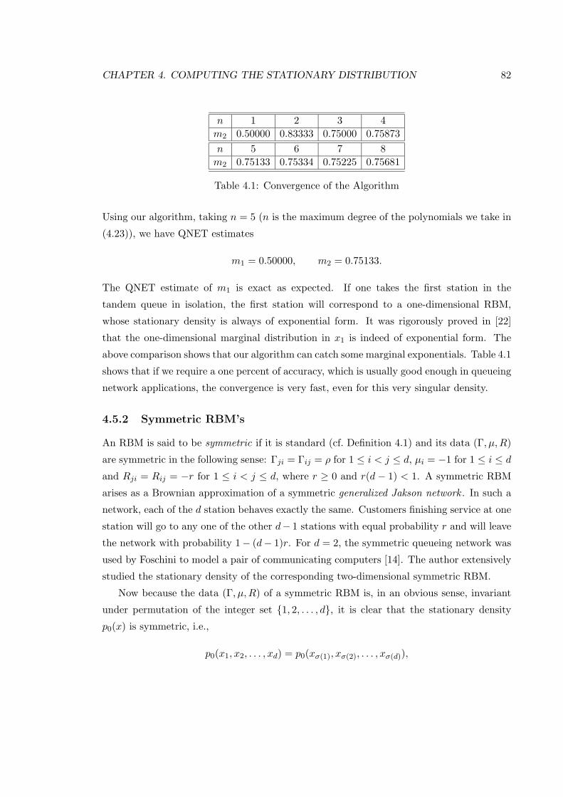
CHAPTER 4. COMPUTING THE STATIONARY DISTRIBUTION 82
n 1 2 3 4m2 0.50000 0.83333 0.75000 0.75873n 5 6 7 8m2 0.75133 0.75334 0.75225 0.75681
Table 4.1: Convergence of the Algorithm
Using our algorithm, taking n = 5 (n is the maximum degree of the polynomials we take in
(4.23)), we have QNET estimates
m1 = 0.50000, m2 = 0.75133.
The QNET estimate of m1 is exact as expected. If one takes the first station in the
tandem queue in isolation, the first station will correspond to a one-dimensional RBM,
whose stationary density is always of exponential form. It was rigorously proved in [22]
that the one-dimensional marginal distribution in x1 is indeed of exponential form. The
above comparison shows that our algorithm can catch some marginal exponentials. Table 4.1
shows that if we require a one percent of accuracy, which is usually good enough in queueing
network applications, the convergence is very fast, even for this very singular density.
4.5.2 Symmetric RBM’s
An RBM is said to be symmetric if it is standard (cf. Definition 4.1) and its data (Γ, µ,R)
are symmetric in the following sense: Γji = Γij = ρ for 1 ≤ i < j ≤ d, µi = −1 for 1 ≤ i ≤ dand Rji = Rij = −r for 1 ≤ i < j ≤ d, where r ≥ 0 and r(d − 1) < 1. A symmetric RBM
arises as a Brownian approximation of a symmetric generalized Jakson network . In such a
network, each of the d station behaves exactly the same. Customers finishing service at one
station will go to any one of the other d− 1 stations with equal probability r and will leave
the network with probability 1− (d− 1)r. For d = 2, the symmetric queueing network was
used by Foschini to model a pair of communicating computers [14]. The author extensively
studied the stationary density of the corresponding two-dimensional symmetric RBM.
Now because the data (Γ, µ,R) of a symmetric RBM is, in an obvious sense, invariant
under permutation of the integer set 1, 2, . . . , d, it is clear that the stationary density
p0(x) is symmetric, i.e.,
p0(x1, x2, . . . , xd) = p0(xσ(1), xσ(2), . . . , xσ(d)),
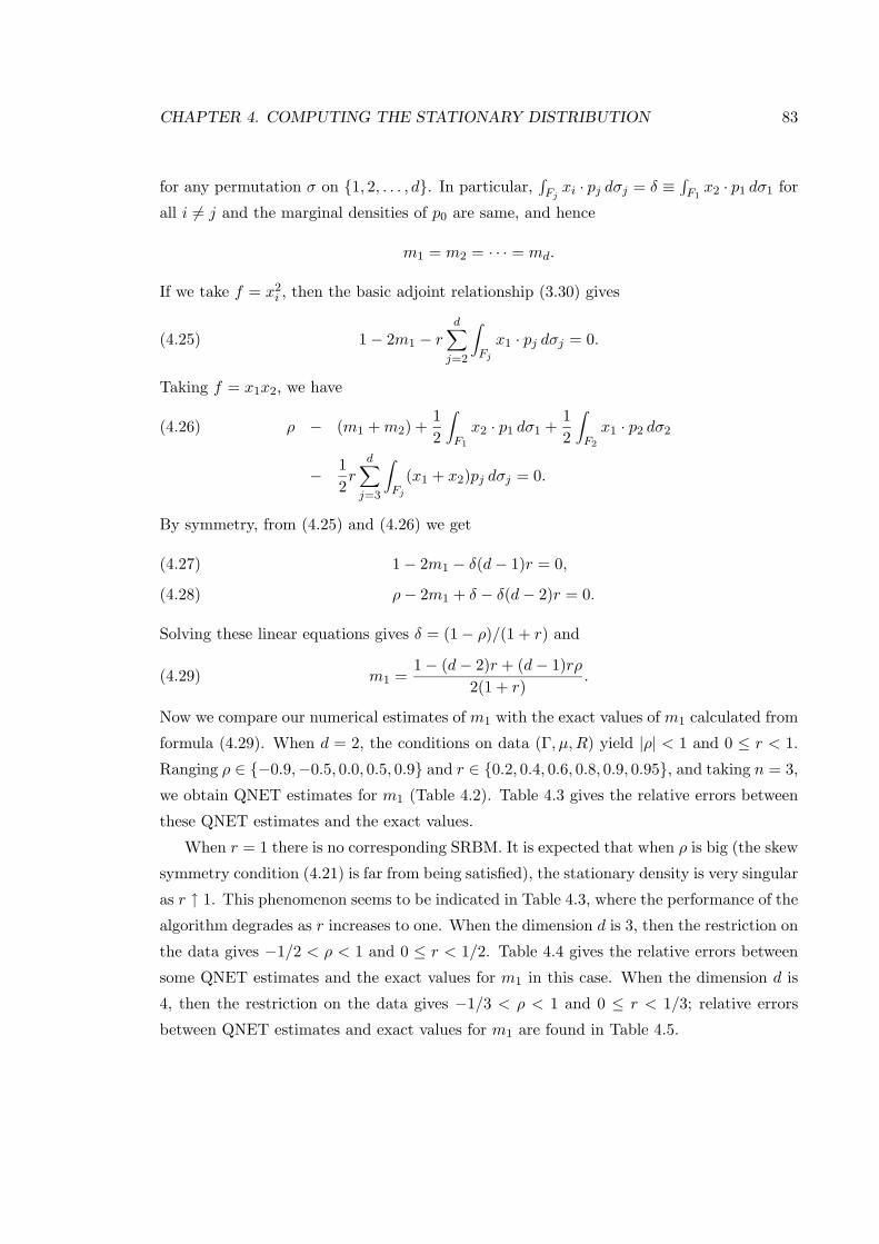
CHAPTER 4. COMPUTING THE STATIONARY DISTRIBUTION 83
for any permutation σ on 1, 2, . . . , d. In particular,∫Fjxi · pj dσj = δ ≡
∫F1x2 · p1 dσ1 for
all i 6= j and the marginal densities of p0 are same, and hence
m1 = m2 = · · · = md.
If we take f = x2i , then the basic adjoint relationship (3.30) gives
1− 2m1 − rd∑j=2
∫Fj
x1 · pj dσj = 0.(4.25)
Taking f = x1x2, we have
ρ − (m1 +m2) +12
∫F1
x2 · p1 dσ1 +12
∫F2
x1 · p2 dσ2(4.26)
− 12r
d∑j=3
∫Fj
(x1 + x2)pj dσj = 0.
By symmetry, from (4.25) and (4.26) we get
1− 2m1 − δ(d− 1)r = 0,(4.27)
ρ− 2m1 + δ − δ(d− 2)r = 0.(4.28)
Solving these linear equations gives δ = (1− ρ)/(1 + r) and
m1 =1− (d− 2)r + (d− 1)rρ
2(1 + r).(4.29)
Now we compare our numerical estimates of m1 with the exact values of m1 calculated from
formula (4.29). When d = 2, the conditions on data (Γ, µ,R) yield |ρ| < 1 and 0 ≤ r < 1.
Ranging ρ ∈ −0.9,−0.5, 0.0, 0.5, 0.9 and r ∈ 0.2, 0.4, 0.6, 0.8, 0.9, 0.95, and taking n = 3,
we obtain QNET estimates for m1 (Table 4.2). Table 4.3 gives the relative errors between
these QNET estimates and the exact values.
When r = 1 there is no corresponding SRBM. It is expected that when ρ is big (the skew
symmetry condition (4.21) is far from being satisfied), the stationary density is very singular
as r ↑ 1. This phenomenon seems to be indicated in Table 4.3, where the performance of the
algorithm degrades as r increases to one. When the dimension d is 3, then the restriction on
the data gives −1/2 < ρ < 1 and 0 ≤ r < 1/2. Table 4.4 gives the relative errors between
some QNET estimates and the exact values for m1 in this case. When the dimension d is
4, then the restriction on the data gives −1/3 < ρ < 1 and 0 ≤ r < 1/3; relative errors
between QNET estimates and exact values for m1 are found in Table 4.5.
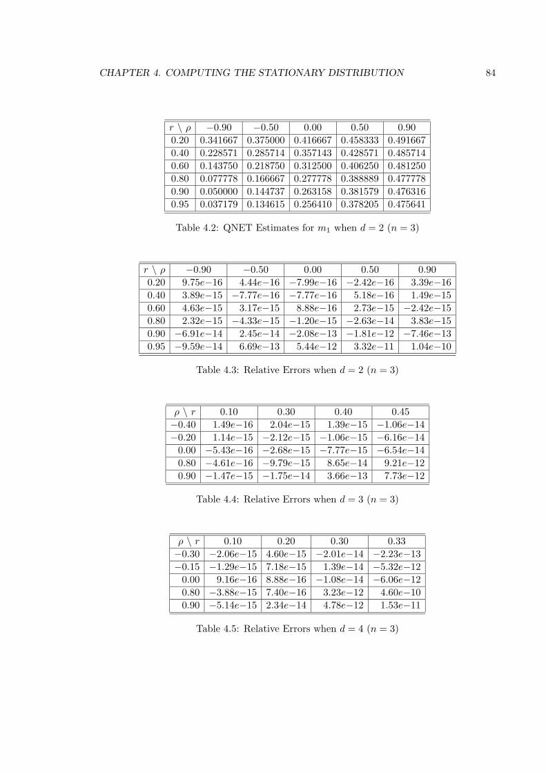
CHAPTER 4. COMPUTING THE STATIONARY DISTRIBUTION 84
r \ ρ −0.90 −0.50 0.00 0.50 0.900.20 0.341667 0.375000 0.416667 0.458333 0.4916670.40 0.228571 0.285714 0.357143 0.428571 0.4857140.60 0.143750 0.218750 0.312500 0.406250 0.4812500.80 0.077778 0.166667 0.277778 0.388889 0.4777780.90 0.050000 0.144737 0.263158 0.381579 0.4763160.95 0.037179 0.134615 0.256410 0.378205 0.475641
Table 4.2: QNET Estimates for m1 when d = 2 (n = 3)
r \ ρ −0.90 −0.50 0.00 0.50 0.900.20 9.75e−16 4.44e−16 −7.99e−16 −2.42e−16 3.39e−160.40 3.89e−15 −7.77e−16 −7.77e−16 5.18e−16 1.49e−150.60 4.63e−15 3.17e−15 8.88e−16 2.73e−15 −2.42e−150.80 2.32e−15 −4.33e−15 −1.20e−15 −2.63e−14 3.83e−150.90 −6.91e−14 2.45e−14 −2.08e−13 −1.81e−12 −7.46e−130.95 −9.59e−14 6.69e−13 5.44e−12 3.32e−11 1.04e−10
Table 4.3: Relative Errors when d = 2 (n = 3)
ρ \ r 0.10 0.30 0.40 0.45−0.40 1.49e−16 2.04e−15 1.39e−15 −1.06e−14−0.20 1.14e−15 −2.12e−15 −1.06e−15 −6.16e−14
0.00 −5.43e−16 −2.68e−15 −7.77e−15 −6.54e−140.80 −4.61e−16 −9.79e−15 8.65e−14 9.21e−120.90 −1.47e−15 −1.75e−14 3.66e−13 7.73e−12
Table 4.4: Relative Errors when d = 3 (n = 3)
ρ \ r 0.10 0.20 0.30 0.33−0.30 −2.06e−15 4.60e−15 −2.01e−14 −2.23e−13−0.15 −1.29e−15 7.18e−15 1.39e−14 −5.32e−12
0.00 9.16e−16 8.88e−16 −1.08e−14 −6.06e−120.80 −3.88e−15 7.40e−16 3.23e−12 4.60e−100.90 −5.14e−15 2.34e−14 4.78e−12 1.53e−11
Table 4.5: Relative Errors when d = 4 (n = 3)
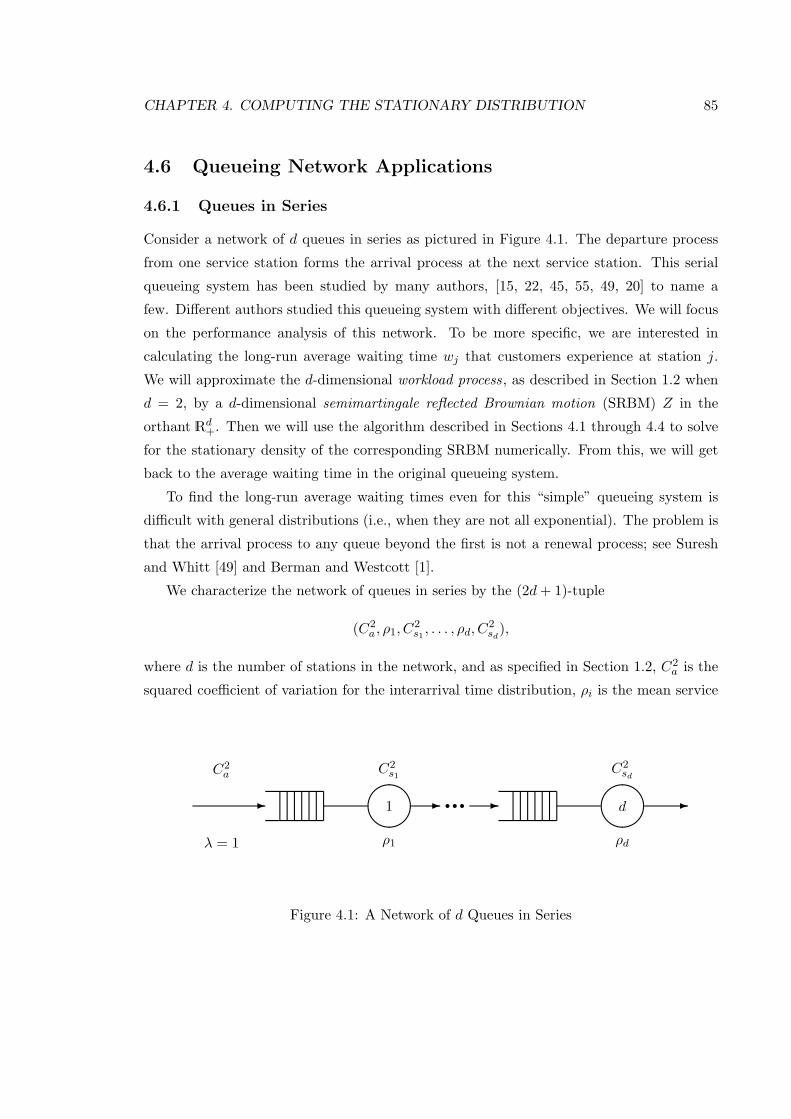
CHAPTER 4. COMPUTING THE STATIONARY DISTRIBUTION 85
4.6 Queueing Network Applications
4.6.1 Queues in Series
Consider a network of d queues in series as pictured in Figure 4.1. The departure process
from one service station forms the arrival process at the next service station. This serial
queueing system has been studied by many authors, [15, 22, 45, 55, 49, 20] to name a
few. Different authors studied this queueing system with different objectives. We will focus
on the performance analysis of this network. To be more specific, we are interested in
calculating the long-run average waiting time wj that customers experience at station j.
We will approximate the d-dimensional workload process, as described in Section 1.2 when
d = 2, by a d-dimensional semimartingale reflected Brownian motion (SRBM) Z in the
orthant Rd+. Then we will use the algorithm described in Sections 4.1 through 4.4 to solve
for the stationary density of the corresponding SRBM numerically. From this, we will get
back to the average waiting time in the original queueing system.
To find the long-run average waiting times even for this “simple” queueing system is
difficult with general distributions (i.e., when they are not all exponential). The problem is
that the arrival process to any queue beyond the first is not a renewal process; see Suresh
and Whitt [49] and Berman and Westcott [1].
We characterize the network of queues in series by the (2d+ 1)-tuple
(C2a , ρ1, C
2s1 , . . . , ρd, C
2sd
),
where d is the number of stations in the network, and as specified in Section 1.2, C2a is the
squared coefficient of variation for the interarrival time distribution, ρi is the mean service
C2a
-
λ = 1
C2s1
1
ρ1
- r r r -C2sd
d
ρd
-
Figure 4.1: A Network of d Queues in Series
CHAPTER 4. COMPUTING THE STATIONARY DISTRIBUTION 86
time at station i and C2si is the squared coefficient of variation of the service time distribution
at station i. We assume the arrival rate to station 1 is one so that ρi is the traffic intensity
at station i. Using the method proposed in Harrison and Nguyen [24], as illustrated in
Section 1.2, the d-dimensional current workload process W (t) = (W1(t), . . . ,Wd(t))′ can be
replaced (approximated) by a d-dimensional SRBM Z in the orthant Rd+ associated with
data (Γ, µ,R). When d = 2, it has been derived in Section 1.2 that
Γ =
ρ21(C2
a + C2s1) −ρ1ρ2C
2s1
−ρ1ρ2C2s1 ρ2
2(C2s1 + C2
s2)
, µ =
ρ1 − 1
ρ2/ρ1 − 1
, R =
1 0
−ρ2/ρ1 1,
.Using the algorithm developed in an earlier part of this chapter, we can calculate the steady
state mean m = (m1,m2, . . . ,md)′ of Z. It is suggested in [24] that the expected waiting
times w = (w1, . . . , wd)′ be approximated by the long-run average workload levels, and
hence we have the estimates
wj.= mj , j = 1, . . . , d.
In the following, we will compare our QNET estimates of average waiting times for
many system configurations and a variety of system parameters with simulation estimates
as well as with estimates from other approximation schemes. Readers should notice that in
using QNET to estimate w, there are two levels of errors that might occur. The first level
comes from the model replacement (wj.= mj), and the second level of error comes from the
numerical calculation of mj .
Fraker’s Experiment
Here we consider Fraker’s [15] experiment. Fraker simulated eight different cases of eight
single-server queues in series. In all cases, the external arrival process is Possion, and
all service time distributions are Erlang. Each of four traffic intensities (ρ = 0.3, 0.5, 0.7
and 0.9) and each of four Erlang service-time distributions (M = E1, E4, E8, and D =
E∞) is assigned randomly to two of the eight nodes (M for exponential distributions or
memoryless, and D for deterministic). Fraker’s simulations consisted of three separate runs
of 2500 customers each, with the first 500 being discarded to damp out the transient effects.
Statistics were collected for six blocks of 1000 customers each. As pointed out by Whitt
[55], the simulation runs were not long enough for good statistical accuracy, and no single
estimate can be relied upon, but the total experiment clearly yields meaningful comparisons
of approximations.
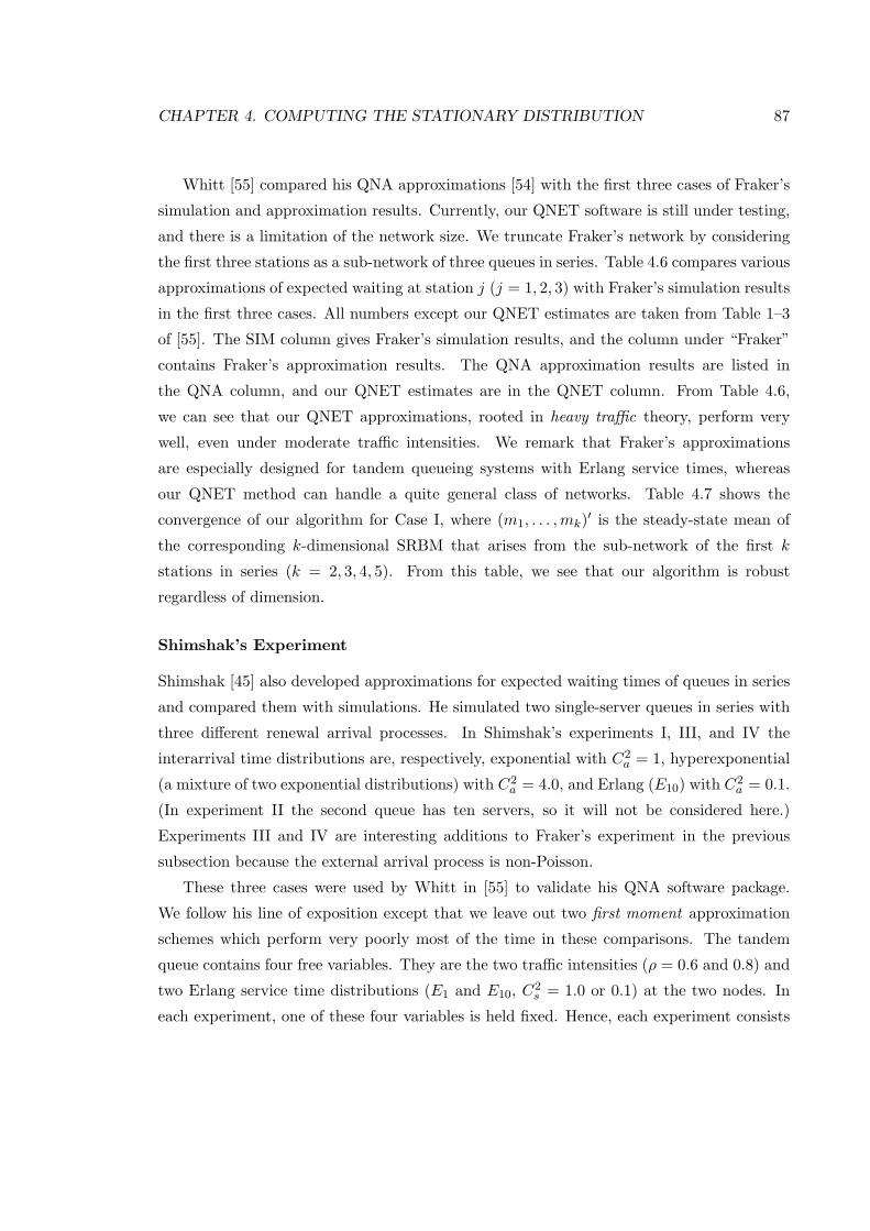
CHAPTER 4. COMPUTING THE STATIONARY DISTRIBUTION 87
Whitt [55] compared his QNA approximations [54] with the first three cases of Fraker’s
simulation and approximation results. Currently, our QNET software is still under testing,
and there is a limitation of the network size. We truncate Fraker’s network by considering
the first three stations as a sub-network of three queues in series. Table 4.6 compares various
approximations of expected waiting at station j (j = 1, 2, 3) with Fraker’s simulation results
in the first three cases. All numbers except our QNET estimates are taken from Table 1–3
of [55]. The SIM column gives Fraker’s simulation results, and the column under “Fraker”
contains Fraker’s approximation results. The QNA approximation results are listed in
the QNA column, and our QNET estimates are in the QNET column. From Table 4.6,
we can see that our QNET approximations, rooted in heavy traffic theory, perform very
well, even under moderate traffic intensities. We remark that Fraker’s approximations
are especially designed for tandem queueing systems with Erlang service times, whereas
our QNET method can handle a quite general class of networks. Table 4.7 shows the
convergence of our algorithm for Case I, where (m1, . . . ,mk)′ is the steady-state mean of
the corresponding k-dimensional SRBM that arises from the sub-network of the first k
stations in series (k = 2, 3, 4, 5). From this table, we see that our algorithm is robust
regardless of dimension.
Shimshak’s Experiment
Shimshak [45] also developed approximations for expected waiting times of queues in series
and compared them with simulations. He simulated two single-server queues in series with
three different renewal arrival processes. In Shimshak’s experiments I, III, and IV the
interarrival time distributions are, respectively, exponential with C2a = 1, hyperexponential
(a mixture of two exponential distributions) with C2a = 4.0, and Erlang (E10) with C2
a = 0.1.
(In experiment II the second queue has ten servers, so it will not be considered here.)
Experiments III and IV are interesting additions to Fraker’s experiment in the previous
subsection because the external arrival process is non-Poisson.
These three cases were used by Whitt in [55] to validate his QNA software package.
We follow his line of exposition except that we leave out two first moment approximation
schemes which perform very poorly most of the time in these comparisons. The tandem
queue contains four free variables. They are the two traffic intensities (ρ = 0.6 and 0.8) and
two Erlang service time distributions (E1 and E10, C2s = 1.0 or 0.1) at the two nodes. In
each experiment, one of these four variables is held fixed. Hence, each experiment consists
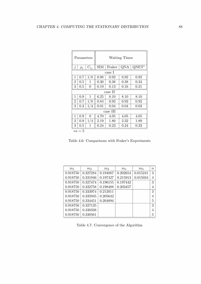
CHAPTER 4. COMPUTING THE STATIONARY DISTRIBUTION 88
Parameters Waiting Times
j ρj Csj SIM Fraker QNA QNET∗
case I1 0.7 1/8 0.98 0.92 0.92 0.922 0.5 1 0.30 0.38 0.38 0.343 0.5 0 0.19 0.13 0.16 0.21
case II1 0.9 1 6.25 8.10 8.10 8.102 0.7 1/8 0.84 0.92 0.92 0.923 0.3 1/4 0.01 0.04 0.04 0.03
case III1 0.9 0 4.70 4.05 4.05 4.052 0.9 1/4 2.19 1.80 2.32 1.893 0.5 1 0.24 0.23 0.24 0.33∗n = 5
Table 4.6: Comparisons with Fraker’s Experiments
m1 m2 m3 m4 m5 n
0.918750 0.327284 0.194887 0.202654 0.015241 30.918750 0.331946 0.197427 0.215913 0.015034 40.918750 0.327474 0.196155 0.197442 30.918750 0.332758 0.198488 0.203457 40.918750 0.333974 0.212011 30.918750 0.335945 0.205642 40.918750 0.334451 0.204894 50.918750 0.327135 30.918750 0.330338 40.918750 0.330561 5
Table 4.7: Convergence of the Algorithm
CHAPTER 4. COMPUTING THE STATIONARY DISTRIBUTION 89
of eight cases, containing all combinations of three variables, each with two possible values.
In experiment I the service time distribution at node 1 is always E10; in experiments III
and IV the traffic intensity at node 1 is always 0.8.
Shimshak’s simulations were obtained using GPSS and the regenerative method. The
number of customers simulated in each case ranged from 15,000 to 25,000, depending on
the traffic intensity. The statistical reliability is indicated by 95% confidence intervals. The
simulation results and the approximations for expected total waiting times appear in Ta-
bles 4.8–4.10. The Fraker, Page and Marchal approximations are approximations devised by
Shimshak using earlier methods. All the numbers except QNET estimates are taken from
Table 6–8 of [55]. The half width of the 95% confidence interval is in parentheses below
the simulation estimates. The estimated relative error appears below the approximation in
parentheses. It is the approximation value minus the simulation value divided by the simu-
lation value. The blanks in the Fraker column in Table 4.9 mean his approximation failed
in these cases. We take n = 6 for our QNET calculations. In Table 4.8, except for Case 7,
our QNET estimates give very good approximations of the total waiting times. In case 7,
the squared coefficient of variation of the interarrivals is C2a = 1, which is big compared to
the squared coefficient of variation of the service times at both stations, C2s1 = C2
s2 = 0.1.
Case 7 in Table 4.8 shows that our QNET method fails to catch the high variability of
the arrival process to the second queue, and therefore underestimates the average waiting
time at the second station. Table 4.9 shows that our QNET approximations are uniformly
better than QNA approximations, whereas in Table 4.10, our QNET approximations fail
to get good approximations at all. Notice that in Table 4.10, for Case 2, Case 4, Case 6
and Case 8, because C2a = C2
s1 = 0.1, there is a product form formula to calculate the
corresponding steady-state mean m. In other words, the QNET calculation for m is exact ,
and all errors come from the model replacement. Presumably, this is due to the fact that
traffic intensities are not high enough, and Table 4.10 confirms this. The rows with the
largest errors have very small waiting times. This suggests that more validation of QNET
is needed.
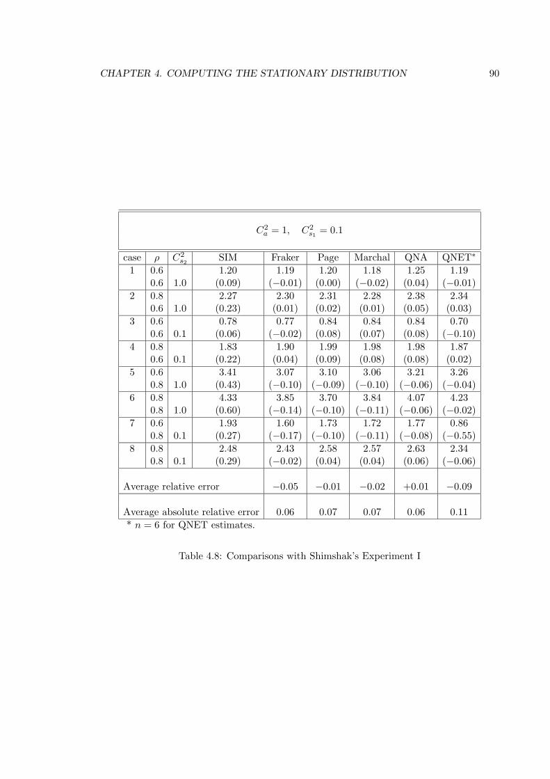
CHAPTER 4. COMPUTING THE STATIONARY DISTRIBUTION 90
C2a = 1, C2
s1 = 0.1
case ρ C2s2 SIM Fraker Page Marchal QNA QNET∗
1 0.6 1.20 1.19 1.20 1.18 1.25 1.190.6 1.0 (0.09) (−0.01) (0.00) (−0.02) (0.04) (−0.01)
2 0.8 2.27 2.30 2.31 2.28 2.38 2.340.6 1.0 (0.23) (0.01) (0.02) (0.01) (0.05) (0.03)
3 0.6 0.78 0.77 0.84 0.84 0.84 0.700.6 0.1 (0.06) (−0.02) (0.08) (0.07) (0.08) (−0.10)
4 0.8 1.83 1.90 1.99 1.98 1.98 1.870.6 0.1 (0.22) (0.04) (0.09) (0.08) (0.08) (0.02)
5 0.6 3.41 3.07 3.10 3.06 3.21 3.260.8 1.0 (0.43) (−0.10) (−0.09) (−0.10) (−0.06) (−0.04)
6 0.8 4.33 3.85 3.70 3.84 4.07 4.230.8 1.0 (0.60) (−0.14) (−0.10) (−0.11) (−0.06) (−0.02)
7 0.6 1.93 1.60 1.73 1.72 1.77 0.860.8 0.1 (0.27) (−0.17) (−0.10) (−0.11) (−0.08) (−0.55)
8 0.8 2.48 2.43 2.58 2.57 2.63 2.340.8 0.1 (0.29) (−0.02) (0.04) (0.04) (0.06) (−0.06)
Average relative error −0.05 −0.01 −0.02 +0.01 −0.09
Average absolute relative error 0.06 0.07 0.07 0.06 0.11* n = 6 for QNET estimates.
Table 4.8: Comparisons with Shimshak’s Experiment I
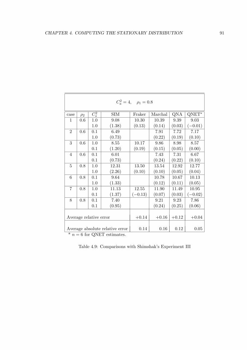
CHAPTER 4. COMPUTING THE STATIONARY DISTRIBUTION 91
C2a = 4, ρ1 = 0.8
case ρ2 C2s SIM Fraker Marchal QNA QNET∗
1 0.6 1.0 9.08 10.30 10.39 9.39 9.031.0 (1.38) (0.13) (0.14) (0.03) (−0.01)
2 0.6 0.1 6.49 7.91 7.72 7.171.0 (0.73) (0.22) (0.19) (0.10)
3 0.6 1.0 8.55 10.17 9.86 8.98 8.570.1 (1.20) (0.19) (0.15) (0.05) (0.00)
4 0.6 0.1 6.01 7.43 7.31 6.670.1 (0.73) (0.24) (0.22) (0.10)
5 0.8 1.0 12.31 13.50 13.54 12.92 12.771.0 (2.26) (0.10) (0.10) (0.05) (0.04)
6 0.8 0.1 9.64 10.78 10.67 10.131.0 (1.33) (0.12) (0.11) (0.05)
7 0.8 1.0 11.13 12.55 11.90 11.49 10.950.1 (1.37) (−0.13) (0.07) (0.03) (−0.02)
8 0.8 0.1 7.40 9.21 9.23 7.860.1 (0.95) (0.24) (0.25) (0.06)
Average relative error +0.14 +0.16 +0.12 +0.04
Average absolute relative error 0.14 0.16 0.12 0.05* n = 6 for QNET estimates.
Table 4.9: Comparisons with Shimshak’s Experiment III
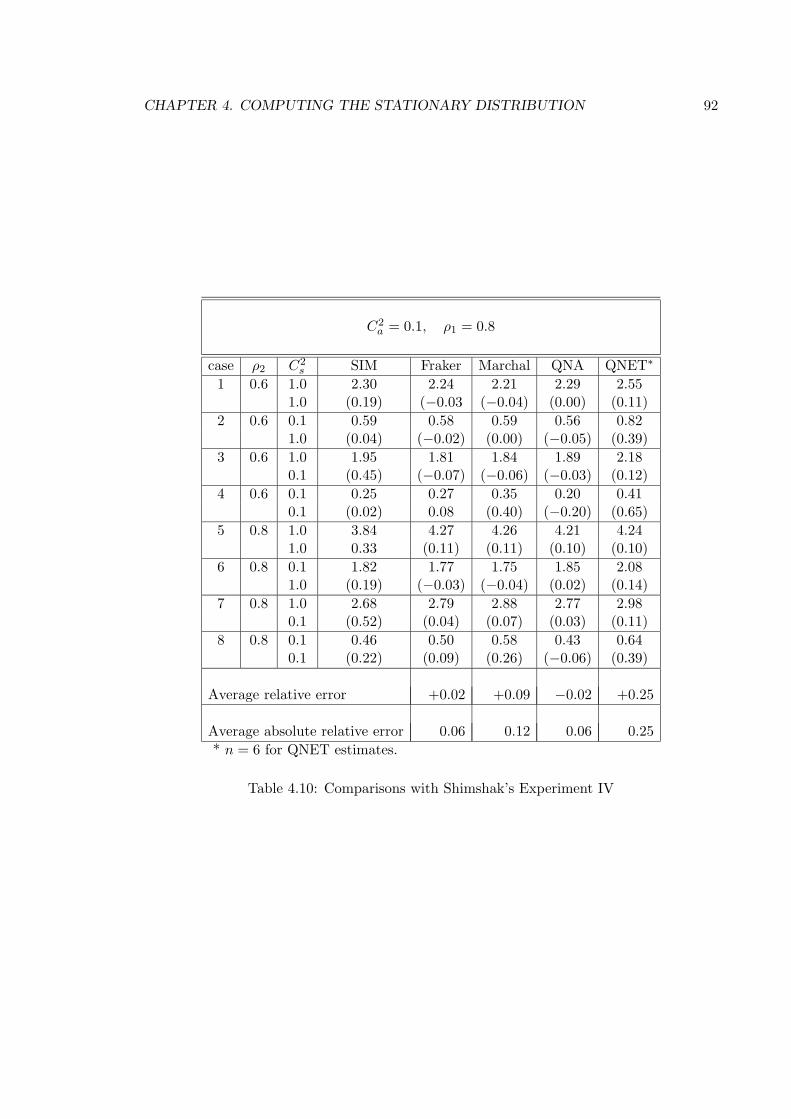
CHAPTER 4. COMPUTING THE STATIONARY DISTRIBUTION 92
C2a = 0.1, ρ1 = 0.8
case ρ2 C2s SIM Fraker Marchal QNA QNET∗
1 0.6 1.0 2.30 2.24 2.21 2.29 2.551.0 (0.19) (−0.03 (−0.04) (0.00) (0.11)
2 0.6 0.1 0.59 0.58 0.59 0.56 0.821.0 (0.04) (−0.02) (0.00) (−0.05) (0.39)
3 0.6 1.0 1.95 1.81 1.84 1.89 2.180.1 (0.45) (−0.07) (−0.06) (−0.03) (0.12)
4 0.6 0.1 0.25 0.27 0.35 0.20 0.410.1 (0.02) 0.08 (0.40) (−0.20) (0.65)
5 0.8 1.0 3.84 4.27 4.26 4.21 4.241.0 0.33 (0.11) (0.11) (0.10) (0.10)
6 0.8 0.1 1.82 1.77 1.75 1.85 2.081.0 (0.19) (−0.03) (−0.04) (0.02) (0.14)
7 0.8 1.0 2.68 2.79 2.88 2.77 2.980.1 (0.52) (0.04) (0.07) (0.03) (0.11)
8 0.8 0.1 0.46 0.50 0.58 0.43 0.640.1 (0.22) (0.09) (0.26) (−0.06) (0.39)
Average relative error +0.02 +0.09 −0.02 +0.25
Average absolute relative error 0.06 0.12 0.06 0.25* n = 6 for QNET estimates.
Table 4.10: Comparisons with Shimshak’s Experiment IV
CHAPTER 4. COMPUTING THE STATIONARY DISTRIBUTION 93
Suresh and Whitt’s Experiment
Recently, Suresh and Whitt [49] did extensive simulations for a network of two queues in
tandem. Their objective is to find a best order of two queues to minimize the average total
waiting time, or equivalently to minimize the average sojourn time. They also compare their
simulations with QNA approximations. For the purpose of this section, we are interested
in comparing simulation results and approximation results for the expected waiting time at
the second station only, because, in both QNA and QNET, the expected waiting time at
the first station is approximated by Kingman’s heavy traffic formula
w1 = ρ1
(ρ1
1− ρ1
)(C2a + C2
s1
2
),
which has been tested intensively and found to be relatively good, see [54]. If the departure
process from station 1 were a renewal process and its squared coefficient of variation C2d
could be calculated in some way, Kingman’s formula could be used again to yield an estimate
for the expected waiting at the second station. Unfortunately, the arrival process to the
second queue (or the departure process from the first queue) is typically not renewal, see [49]
and Berman and Westcott [1]. It is this difficulty which is challenging queueing performance
analysts, and Whitt’s QNA is trying to overcome the difficulty. The QNET method now
provides another way for us to estimate the expected waiting at the second station. We
should emphasize that QNET can do more in this respect, that is, it gives an approximation
of the joint densities of the waiting times at the two stations.
Suresh and Whitt used the SIMAN simulation program to get the simulation estimates
of the expected steady-state waiting times. In each case, they performed ten independent
replications, using 30,000 arrivals in each replication, and they estimated 90% confidence
intervals using t-statistics. An initial portion of each run (2000 customers) was discarded
to allow the system to approach steady state. They considered various variability pa-
rameter triples (C2a , C
2s1 , C
2s2) for all combinations of the traffic intensities ρ1 and ρ2 in a
representative range. For C2s1 6= C2
s2 they considered five variability triples (C2a , C
2s1 , C
2s2),
namely, (0.5, 0.5, 2.0), (1.0, 0.5, 8.0), (1.0, 2.0, 4.0), (4.0, 0.5, 1.0) and (4.0, 1.0, 4.0), ordered
lexicographically; we will refer to them as Case 1, Case 2, Case 3, Case 4 and Case 5,
respectively. For C2s1 = C2
s2 , they considered two variability triples (C2a , C
2s1 , C
2s2), namely,
(1.0, 0.5, 0.5) and (1.0, 4.0, 4.0); we refer to them as Case 6 and Case 7. When C2s1 6= C2
s2 ,
for each queue they considered four values of ρi: 0.3, 0.6, 0.8, 0.9. Thus, associated with
each variability triple are 32 cases of two queues in series:
CHAPTER 4. COMPUTING THE STATIONARY DISTRIBUTION 94
(4 values of ρ1)× (4 values of ρ2)× (2 orders) = 32 cases.
When C2s1 = C2
s2 , they consider five values of ρi: 0.1, 0.2, 0.3, 0.6 and 0.9. Thus for each triple
there are 15 cases of two queues in series (they consider only ρ1 6= ρ2, because otherwise
the order does not matter).
When C2 = 0.5, the E2 distribution (Erlang of order 2, the convolution of two exponen-
tials) is used in the simulation; when C2 = 1.0, the exponential (M) distribution is used;
when C2 > 1, the H2 distribution (hyperexponential, a mixture of two exponentials) with
balanced means is used. Tables 4.11–4.17 give simulation estimates, Whitt’s QNA estimates
and QNET estimates of the average waiting time at the second station for all seven cases
and two orders. In all tables, “Order I” refers to the given triple, and “Order II” is the
reverse order. “Di” denotes the difference between the approximation and the simulation
estimate. This difference is the minimum of the absolute difference and the absolute relative
difference, where
absolute relative difference =|approximation− simulation estimate|
simulation estimate.
“D1” stands for QNET difference, and “D2” stands for QNA difference. We take n = 5 for
all QNET estimates. The estimated 90% confidence interval appears below the simulation
estimate in each case. From Table 4.11-4.17, we see that except for Table 4.14 (Case 5), the
QNET estimates give very good approximations most of the time. In situation (Order II of
Case 2), the overall QNET estimates are not best, but still under heavy traffic (ρ1, ρ2 ≥ 0.8),
the QNET estimates are much better than the QNA approximations. This confirms the so
called “heavy traffic theory”, which asserts that QNET estimates are “good” under heavy
traffic. These Tables clearly demonstrate that even under moderate traffic intensities, the
QNET estimates are still good, and Table 4.16-4.17 show that QNET performs surprising
well under low traffic intensities.
In Table 4.14, QNET performs very badly when the traffic intensities are not heavy or
are unbalanced heavy. In fact, from Table 4.14, we see that in “Order I” (similarly in “Order
II”, when ρ1 ≥ ρ2), station 1 is heavier loaded than station 2. The high variability of the
arrival process to station 1 is smoothed out to a certain extent, and QNET is able to catch
the correct variability for the arrival process to the second station. When ρ1 < ρ2, QNET
performs badly. At this point, we do not know exactly why this happens. Intuitively, the
first station is lightly loaded, and service time variability is small, therefore, customers need
almost no waiting at station 1, get serviced with low variability and go to the second queue.
CHAPTER 4. COMPUTING THE STATIONARY DISTRIBUTION 95
Therefore, the high variability of the arrival process to station 1 is carried over to the arrival
process to station 2, see Reiman [40]. Somehow, QNET fails to catch this high variability
of the arrival process to the second station and significantly underestimates the expected
waiting time at the second station. This again demonstrate the need for more validation
of the QNET method. Table 4.18 aggregates all balanced heavy traffic cases and gives an
overall comparison of QNET estimates with QNA estimates under heavy traffic. It is clear
from this table that QNET approximations are much better than QNA approximations
under balanced heavy traffic conditions.
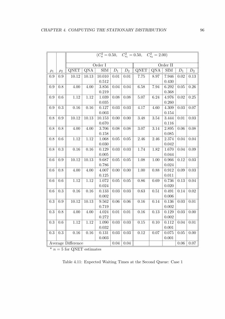
CHAPTER 4. COMPUTING THE STATIONARY DISTRIBUTION 96
(C2a = 0.50, C2
s1 = 0.50, C2s2 = 2.00)
Order I Order IIρ1 ρ2 QNET QNA SIM D1 D2 QNET QNA SIM D1 D2
0.9 0.9 10.12 10.13 10.010 0.01 0.01 7.75 8.97 7.946 0.02 0.130.512 0.430
0.9 0.8 4.00 4.00 3.856 0.04 0.04 6.58 7.94 6.292 0.05 0.260.219 0.368
0.9 0.6 1.12 1.12 1.039 0.08 0.08 5.07 6.24 4.976 0.02 0.250.035 0.260
0.9 0.3 0.16 0.16 0.127 0.03 0.03 4.17 4.60 4.309 0.03 0.070.003 0.154
0.8 0.9 10.12 10.13 10.153 0.00 0.00 3.48 3.54 3.444 0.01 0.030.670 0.116
0.8 0.8 4.00 4.00 3.706 0.08 0.08 3.07 3.14 2.895 0.06 0.080.158 0.085
0.8 0.6 1.12 1.12 1.068 0.05 0.05 2.46 2.46 2.374 0.04 0.040.030 0.042
0.8 0.3 0.16 0.16 0.129 0.03 0.03 1.74 1.82 1.670 0.04 0.090.005 0.044
0.6 0.9 10.12 10.13 9.687 0.05 0.05 1.08 1.00 0.966 0.12 0.030.786 0.024
0.6 0.8 4.00 4.00 4.007 0.00 0.00 1.00 0.88 0.912 0.09 0.030.125 0.011
0.6 0.6 1.12 1.12 1.072 0.05 0.05 0.86 0.69 0.736 0.13 0.040.024 0.020
0.6 0.3 0.16 0.16 0.133 0.03 0.03 0.63 0.51 0.491 0.14 0.020.002 0.006
0.3 0.9 10.12 10.13 9.562 0.06 0.06 0.16 0.14 0.136 0.03 0.010.719 0.002
0.3 0.8 4.00 4.00 4.024 0.01 0.01 0.16 0.13 0.129 0.03 0.000.272 0.002
0.3 0.6 1.12 1.12 1.090 0.03 0.03 0.15 0.10 0.112 0.04 0.010.032 0.001
0.3 0.3 0.16 0.16 0.131 0.03 0.03 0.12 0.07 0.075 0.05 0.000.003 0.001
Average Difference 0.04 0.04 0.06 0.07* n = 5 for QNET estimates
Table 4.11: Expected Waiting Times at the Second Queue: Case 1
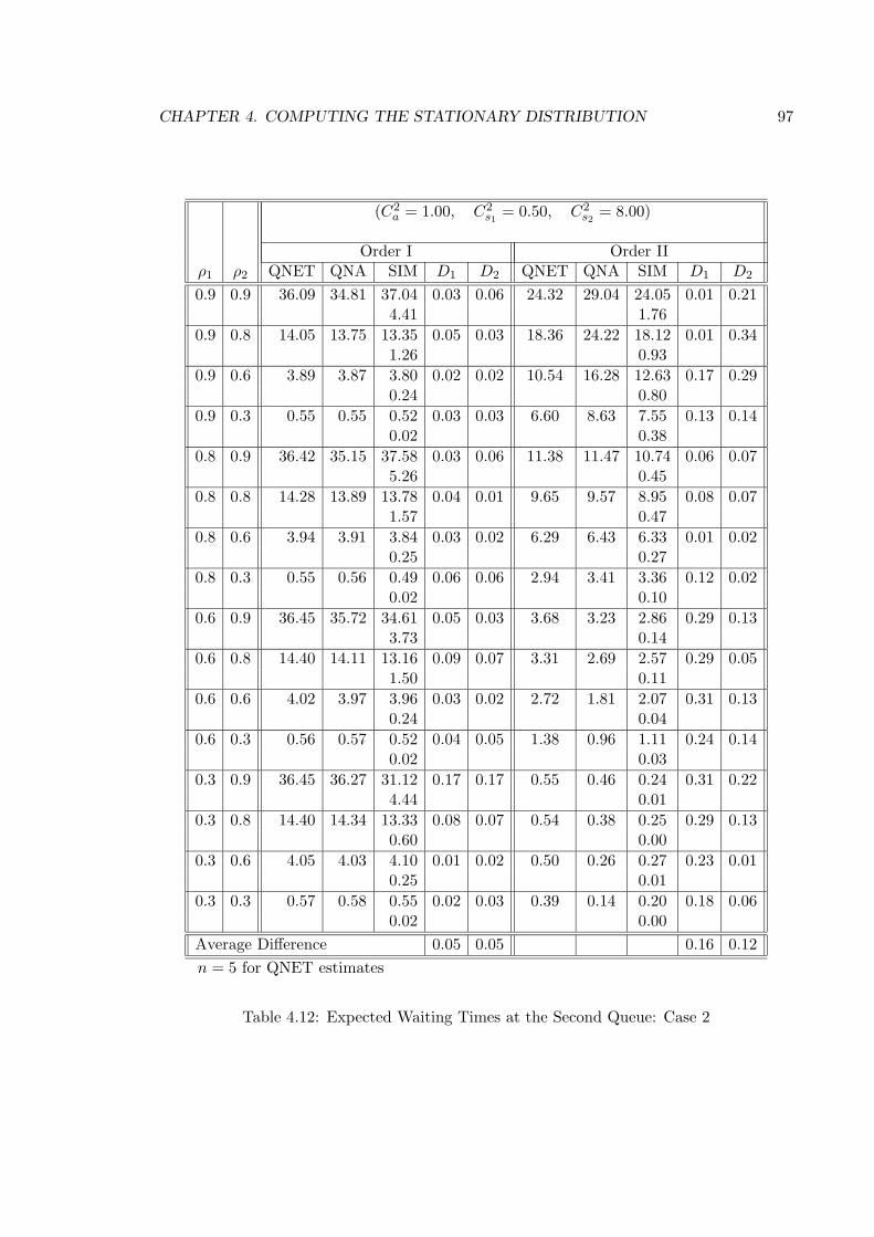
CHAPTER 4. COMPUTING THE STATIONARY DISTRIBUTION 97
(C2a = 1.00, C2
s1 = 0.50, C2s2 = 8.00)
Order I Order IIρ1 ρ2 QNET QNA SIM D1 D2 QNET QNA SIM D1 D2
0.9 0.9 36.09 34.81 37.04 0.03 0.06 24.32 29.04 24.05 0.01 0.214.41 1.76
0.9 0.8 14.05 13.75 13.35 0.05 0.03 18.36 24.22 18.12 0.01 0.341.26 0.93
0.9 0.6 3.89 3.87 3.80 0.02 0.02 10.54 16.28 12.63 0.17 0.290.24 0.80
0.9 0.3 0.55 0.55 0.52 0.03 0.03 6.60 8.63 7.55 0.13 0.140.02 0.38
0.8 0.9 36.42 35.15 37.58 0.03 0.06 11.38 11.47 10.74 0.06 0.075.26 0.45
0.8 0.8 14.28 13.89 13.78 0.04 0.01 9.65 9.57 8.95 0.08 0.071.57 0.47
0.8 0.6 3.94 3.91 3.84 0.03 0.02 6.29 6.43 6.33 0.01 0.020.25 0.27
0.8 0.3 0.55 0.56 0.49 0.06 0.06 2.94 3.41 3.36 0.12 0.020.02 0.10
0.6 0.9 36.45 35.72 34.61 0.05 0.03 3.68 3.23 2.86 0.29 0.133.73 0.14
0.6 0.8 14.40 14.11 13.16 0.09 0.07 3.31 2.69 2.57 0.29 0.051.50 0.11
0.6 0.6 4.02 3.97 3.96 0.03 0.02 2.72 1.81 2.07 0.31 0.130.24 0.04
0.6 0.3 0.56 0.57 0.52 0.04 0.05 1.38 0.96 1.11 0.24 0.140.02 0.03
0.3 0.9 36.45 36.27 31.12 0.17 0.17 0.55 0.46 0.24 0.31 0.224.44 0.01
0.3 0.8 14.40 14.34 13.33 0.08 0.07 0.54 0.38 0.25 0.29 0.130.60 0.00
0.3 0.6 4.05 4.03 4.10 0.01 0.02 0.50 0.26 0.27 0.23 0.010.25 0.01
0.3 0.3 0.57 0.58 0.55 0.02 0.03 0.39 0.14 0.20 0.18 0.060.02 0.00
Average Difference 0.05 0.05 0.16 0.12n = 5 for QNET estimates
Table 4.12: Expected Waiting Times at the Second Queue: Case 2
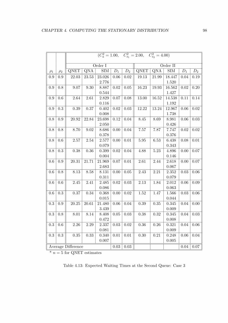
CHAPTER 4. COMPUTING THE STATIONARY DISTRIBUTION 98
(C2a = 1.00, C2
s1 = 2.00, C2s2 = 4.00)
Order I Order IIρ1 ρ2 QNET QNA SIM D1 D2 QNET QNA SIM D1 D2
0.9 0.9 22.03 23.53 23.026 0.06 0.02 19.13 21.99 18.447 0.04 0.192.776 1.520
0.9 0.8 9.07 9.30 8.887 0.02 0.05 16.23 19.93 16.562 0.02 0.200.544 1.427
0.9 0.6 2.64 2.61 2.829 0.07 0.08 13.00 16.52 14.538 0.11 0.140.116 1.192
0.9 0.3 0.39 0.37 0.402 0.02 0.03 12.22 13.24 12.967 0.06 0.020.008 1.738
0.8 0.9 20.92 22.84 23.698 0.12 0.04 8.45 8.69 8.981 0.06 0.032.050 0.426
0.8 0.8 8.70 9.02 8.686 0.00 0.04 7.57 7.87 7.747 0.02 0.020.378 0.376
0.8 0.6 2.57 2.54 2.577 0.00 0.01 5.95 6.53 6.438 0.08 0.010.079 0.343
0.8 0.3 0.38 0.36 0.399 0.02 0.04 4.88 5.23 4.896 0.00 0.070.004 0.146
0.6 0.9 20.31 21.71 21.969 0.07 0.01 2.61 2.44 2.618 0.00 0.072.683 0.067
0.6 0.8 8.13 8.58 8.131 0.00 0.05 2.43 2.21 2.352 0.03 0.060.311 0.079
0.6 0.6 2.45 2.41 2.485 0.02 0.03 2.13 1.84 2.012 0.06 0.090.086 0.063
0.6 0.3 0.37 0.34 0.368 0.00 0.02 1.52 1.47 1.566 0.03 0.060.015 0.044
0.3 0.9 20.25 20.61 21.480 0.06 0.04 0.39 0.35 0.345 0.04 0.003.439 0.009
0.3 0.8 8.01 8.14 8.408 0.05 0.03 0.38 0.32 0.345 0.04 0.030.472 0.008
0.3 0.6 2.26 2.29 2.337 0.03 0.02 0.36 0.26 0.321 0.04 0.060.081 0.009
0.3 0.3 0.35 0.33 0.340 0.01 0.01 0.30 0.21 0.248 0.06 0.040.007 0.005
Average Difference 0.03 0.03 0.04 0.07* n = 5 for QNET estimates
Table 4.13: Expected Waiting Times at the Second Queue: Case 3
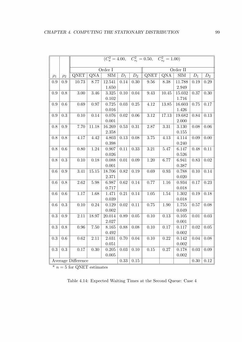
CHAPTER 4. COMPUTING THE STATIONARY DISTRIBUTION 99
(C2a = 4.00, C2
s1 = 0.50, C2s2 = 1.00)
Order I Order IIρ1 ρ2 QNET QNA SIM D1 D2 QNET QNA SIM D1 D2
0.9 0.9 10.73 8.77 12.541 0.14 0.30 9.56 8.38 11.788 0.19 0.291.650 2.949
0.9 0.8 3.00 3.46 3.325 0.10 0.04 9.43 10.45 15.032 0.37 0.300.102 1.716
0.9 0.6 0.69 0.97 0.725 0.03 0.25 4.12 13.85 16.603 0.75 0.170.016 1.426
0.9 0.3 0.10 0.14 0.076 0.02 0.06 3.12 17.13 19.682 0.84 0.130.001 2.000
0.8 0.9 7.70 11.18 16.269 0.53 0.31 2.87 3.31 3.130 0.08 0.062.358 0.155
0.8 0.8 4.17 4.42 4.803 0.13 0.08 3.75 4.13 4.114 0.09 0.000.398 0.240
0.8 0.6 0.80 1.24 0.907 0.11 0.33 3.21 5.47 6.147 0.48 0.110.026 0.526
0.8 0.3 0.10 0.18 0.088 0.01 0.09 1.20 6.77 6.941 0.83 0.020.001 0.387
0.6 0.9 3.41 15.15 18.706 0.82 0.19 0.69 0.93 0.788 0.10 0.142.371 0.020
0.6 0.8 2.62 5.98 6.987 0.62 0.14 0.77 1.16 0.934 0.17 0.230.717 0.018
0.6 0.6 1.17 1.68 1.471 0.21 0.14 1.05 1.54 1.302 0.19 0.180.039 0.018
0.6 0.3 0.10 0.24 0.129 0.02 0.11 0.75 1.90 1.755 0.57 0.080.002 0.049
0.3 0.9 2.11 18.97 20.014 0.89 0.05 0.10 0.13 0.105 0.01 0.032.027 0.001
0.3 0.8 0.96 7.50 8.165 0.88 0.08 0.10 0.17 0.117 0.02 0.050.492 0.002
0.3 0.6 0.62 2.11 2.031 0.70 0.04 0.10 0.22 0.142 0.04 0.080.051 0.002
0.3 0.3 0.17 0.30 0.205 0.03 0.10 0.15 0.27 0.178 0.03 0.090.005 0.002
Average Difference 0.33 0.15 0.30 0.12* n = 5 for QNET estimates
Table 4.14: Expected Waiting Times at the Second Queue: Case 4
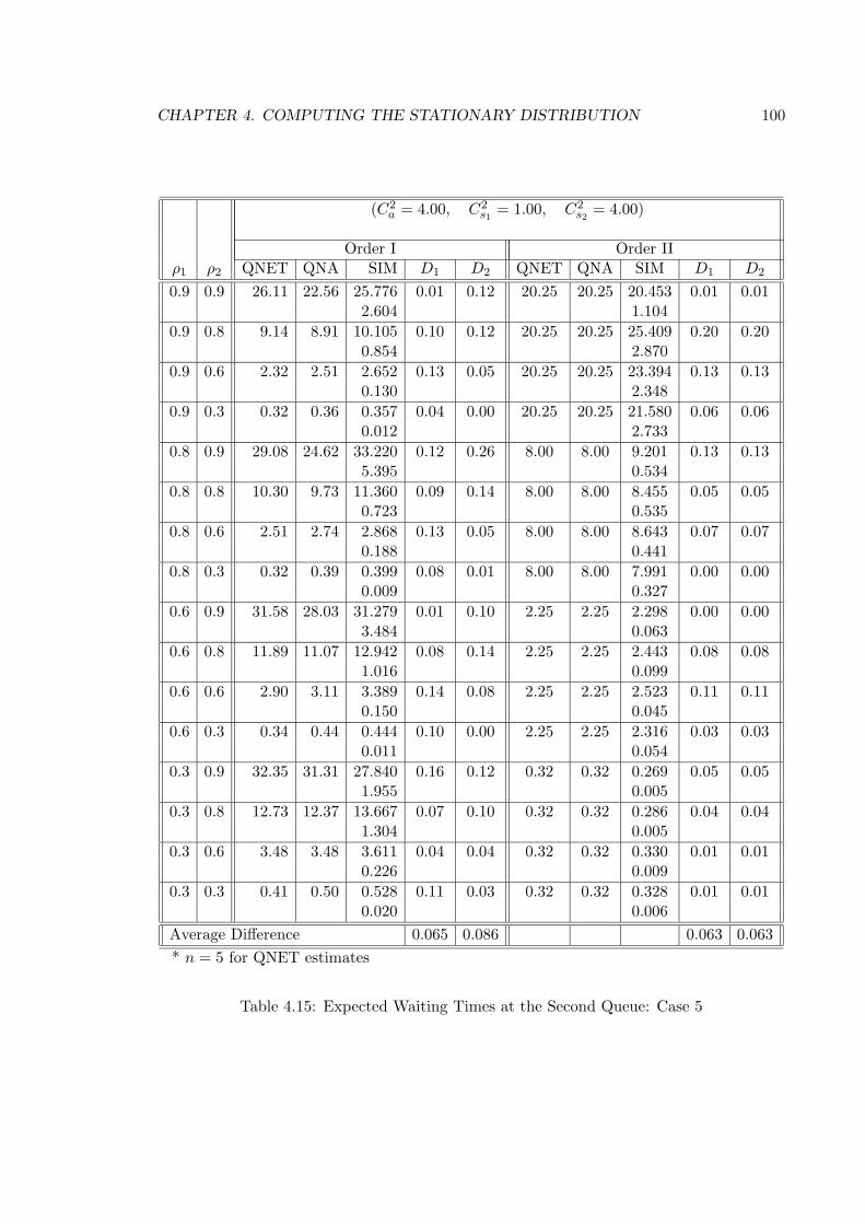
CHAPTER 4. COMPUTING THE STATIONARY DISTRIBUTION 100
(C2a = 4.00, C2
s1 = 1.00, C2s2 = 4.00)
Order I Order IIρ1 ρ2 QNET QNA SIM D1 D2 QNET QNA SIM D1 D2
0.9 0.9 26.11 22.56 25.776 0.01 0.12 20.25 20.25 20.453 0.01 0.012.604 1.104
0.9 0.8 9.14 8.91 10.105 0.10 0.12 20.25 20.25 25.409 0.20 0.200.854 2.870
0.9 0.6 2.32 2.51 2.652 0.13 0.05 20.25 20.25 23.394 0.13 0.130.130 2.348
0.9 0.3 0.32 0.36 0.357 0.04 0.00 20.25 20.25 21.580 0.06 0.060.012 2.733
0.8 0.9 29.08 24.62 33.220 0.12 0.26 8.00 8.00 9.201 0.13 0.135.395 0.534
0.8 0.8 10.30 9.73 11.360 0.09 0.14 8.00 8.00 8.455 0.05 0.050.723 0.535
0.8 0.6 2.51 2.74 2.868 0.13 0.05 8.00 8.00 8.643 0.07 0.070.188 0.441
0.8 0.3 0.32 0.39 0.399 0.08 0.01 8.00 8.00 7.991 0.00 0.000.009 0.327
0.6 0.9 31.58 28.03 31.279 0.01 0.10 2.25 2.25 2.298 0.00 0.003.484 0.063
0.6 0.8 11.89 11.07 12.942 0.08 0.14 2.25 2.25 2.443 0.08 0.081.016 0.099
0.6 0.6 2.90 3.11 3.389 0.14 0.08 2.25 2.25 2.523 0.11 0.110.150 0.045
0.6 0.3 0.34 0.44 0.444 0.10 0.00 2.25 2.25 2.316 0.03 0.030.011 0.054
0.3 0.9 32.35 31.31 27.840 0.16 0.12 0.32 0.32 0.269 0.05 0.051.955 0.005
0.3 0.8 12.73 12.37 13.667 0.07 0.10 0.32 0.32 0.286 0.04 0.041.304 0.005
0.3 0.6 3.48 3.48 3.611 0.04 0.04 0.32 0.32 0.330 0.01 0.010.226 0.009
0.3 0.3 0.41 0.50 0.528 0.11 0.03 0.32 0.32 0.328 0.01 0.010.020 0.006
Average Difference 0.065 0.086 0.063 0.063* n = 5 for QNET estimates
Table 4.15: Expected Waiting Times at the Second Queue: Case 5
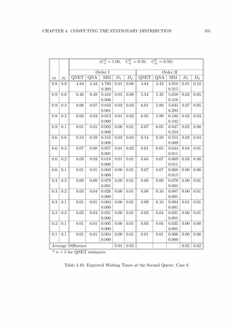
CHAPTER 4. COMPUTING THE STATIONARY DISTRIBUTION 101
(C2a = 1.00, C2
s1 = 0.50, C2s2 = 0.50)
Order I Order IIρ1 ρ2 QNET QNA SIM D1 D2 QNET QNA SIM D1 D2
0.9 0.9 4.84 4.43 4.793 0.01 0.08 4.84 4.43 4.910 0.01 0.100.269 0.215
0.9 0.6 0.46 0.49 0.410 0.05 0.08 5.54 5.35 5.658 0.02 0.050.006 0.410
0.9 0.3 0.06 0.07 0.043 0.02 0.03 6.01 5.89 5.635 0.07 0.050.001 0.293
0.9 0.2 0.03 0.03 0.013 0.01 0.02 6.05 5.99 6.180 0.02 0.030.000 0.442
0.9 0.1 0.01 0.01 0.002 0.00 0.01 6.07 6.05 6.047 0.02 0.000.000 0.253
0.6 0.6 0.54 0.59 0.552 0.02 0.04 0.54 0.59 0.552 0.02 0.040.008 0.009
0.6 0.3 0.07 0.08 0.057 0.01 0.02 0.61 0.65 0.644 0.04 0.010.001 0.011
0.6 0.2 0.03 0.03 0.018 0.01 0.01 0.64 0.67 0.669 0.03 0.000.000 0.011
0.6 0.1 0.01 0.01 0.003 0.00 0.01 0.67 0.67 0.668 0.00 0.000.000 0.015
0.3 0.3 0.08 0.09 0.079 0.00 0.01 0.08 0.09 0.079 0.00 0.010.001 0.001
0.3 0.2 0.03 0.04 0.026 0.00 0.01 0.08 0.10 0.087 0.00 0.010.000 0.001
0.3 0.1 0.01 0.01 0.004 0.00 0.01 0.09 0.10 0.094 0.01 0.010.000 0.001
0.2 0.2 0.03 0.04 0.031 0.00 0.01 0.03 0.04 0.031 0.00 0.010.000 0.001
0.2 0.1 0.01 0.01 0.005 0.00 0.01 0.03 0.04 0.035 0.00 0.000.000 0.001
0.1 0.1 0.01 0.01 0.004 0.00 0.01 0.01 0.01 0.006 0.00 0.000.000 0.000
Average Difference 0.01 0.02 0.02 0.02* n = 5 for QNET estimates
Table 4.16: Expected Waiting Times at the Second Queue: Case 6
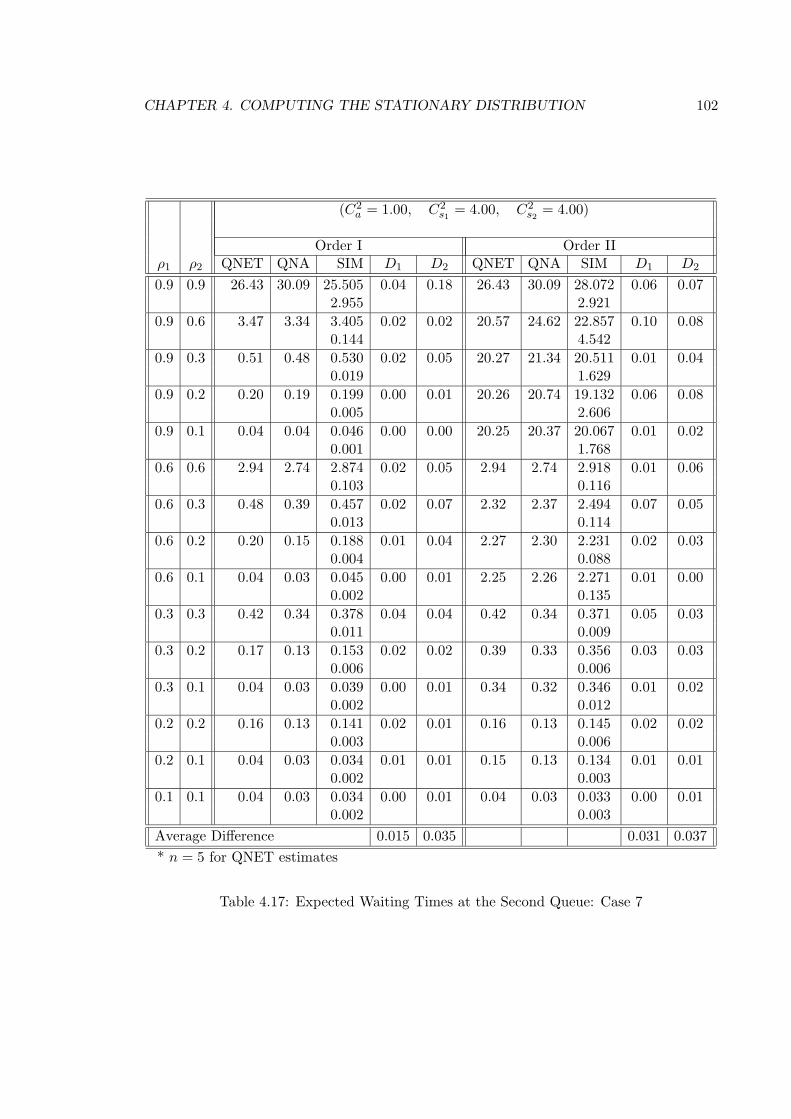
CHAPTER 4. COMPUTING THE STATIONARY DISTRIBUTION 102
(C2a = 1.00, C2
s1 = 4.00, C2s2 = 4.00)
Order I Order IIρ1 ρ2 QNET QNA SIM D1 D2 QNET QNA SIM D1 D2
0.9 0.9 26.43 30.09 25.505 0.04 0.18 26.43 30.09 28.072 0.06 0.072.955 2.921
0.9 0.6 3.47 3.34 3.405 0.02 0.02 20.57 24.62 22.857 0.10 0.080.144 4.542
0.9 0.3 0.51 0.48 0.530 0.02 0.05 20.27 21.34 20.511 0.01 0.040.019 1.629
0.9 0.2 0.20 0.19 0.199 0.00 0.01 20.26 20.74 19.132 0.06 0.080.005 2.606
0.9 0.1 0.04 0.04 0.046 0.00 0.00 20.25 20.37 20.067 0.01 0.020.001 1.768
0.6 0.6 2.94 2.74 2.874 0.02 0.05 2.94 2.74 2.918 0.01 0.060.103 0.116
0.6 0.3 0.48 0.39 0.457 0.02 0.07 2.32 2.37 2.494 0.07 0.050.013 0.114
0.6 0.2 0.20 0.15 0.188 0.01 0.04 2.27 2.30 2.231 0.02 0.030.004 0.088
0.6 0.1 0.04 0.03 0.045 0.00 0.01 2.25 2.26 2.271 0.01 0.000.002 0.135
0.3 0.3 0.42 0.34 0.378 0.04 0.04 0.42 0.34 0.371 0.05 0.030.011 0.009
0.3 0.2 0.17 0.13 0.153 0.02 0.02 0.39 0.33 0.356 0.03 0.030.006 0.006
0.3 0.1 0.04 0.03 0.039 0.00 0.01 0.34 0.32 0.346 0.01 0.020.002 0.012
0.2 0.2 0.16 0.13 0.141 0.02 0.01 0.16 0.13 0.145 0.02 0.020.003 0.006
0.2 0.1 0.04 0.03 0.034 0.01 0.01 0.15 0.13 0.134 0.01 0.010.002 0.003
0.1 0.1 0.04 0.03 0.034 0.00 0.01 0.04 0.03 0.033 0.00 0.010.002 0.003
Average Difference 0.015 0.035 0.031 0.037* n = 5 for QNET estimates
Table 4.17: Expected Waiting Times at the Second Queue: Case 7
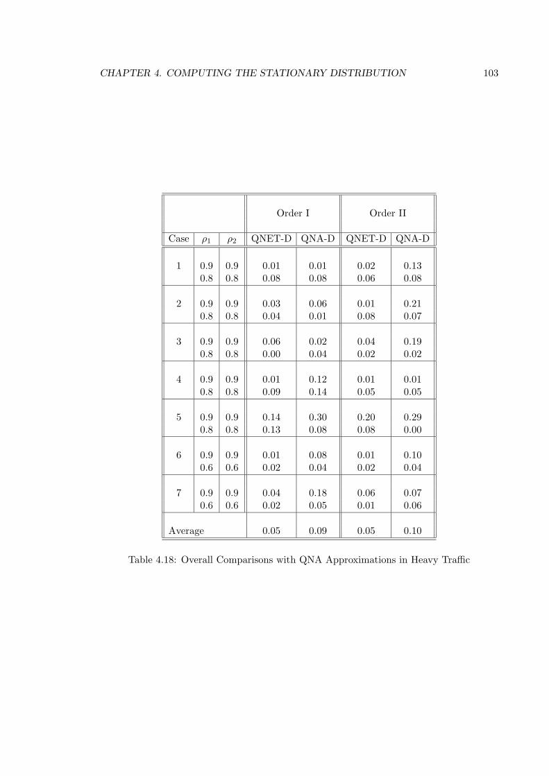
CHAPTER 4. COMPUTING THE STATIONARY DISTRIBUTION 103
Order I Order II
Case ρ1 ρ2 QNET-D QNA-D QNET-D QNA-D
1 0.9 0.9 0.01 0.01 0.02 0.130.8 0.8 0.08 0.08 0.06 0.08
2 0.9 0.9 0.03 0.06 0.01 0.210.8 0.8 0.04 0.01 0.08 0.07
3 0.9 0.9 0.06 0.02 0.04 0.190.8 0.8 0.00 0.04 0.02 0.02
4 0.9 0.9 0.01 0.12 0.01 0.010.8 0.8 0.09 0.14 0.05 0.05
5 0.9 0.9 0.14 0.30 0.20 0.290.8 0.8 0.13 0.08 0.08 0.00
6 0.9 0.9 0.01 0.08 0.01 0.100.6 0.6 0.02 0.04 0.02 0.04
7 0.9 0.9 0.04 0.18 0.06 0.070.6 0.6 0.02 0.05 0.01 0.06
Average 0.05 0.09 0.05 0.10
Table 4.18: Overall Comparisons with QNA Approximations in Heavy Traffic
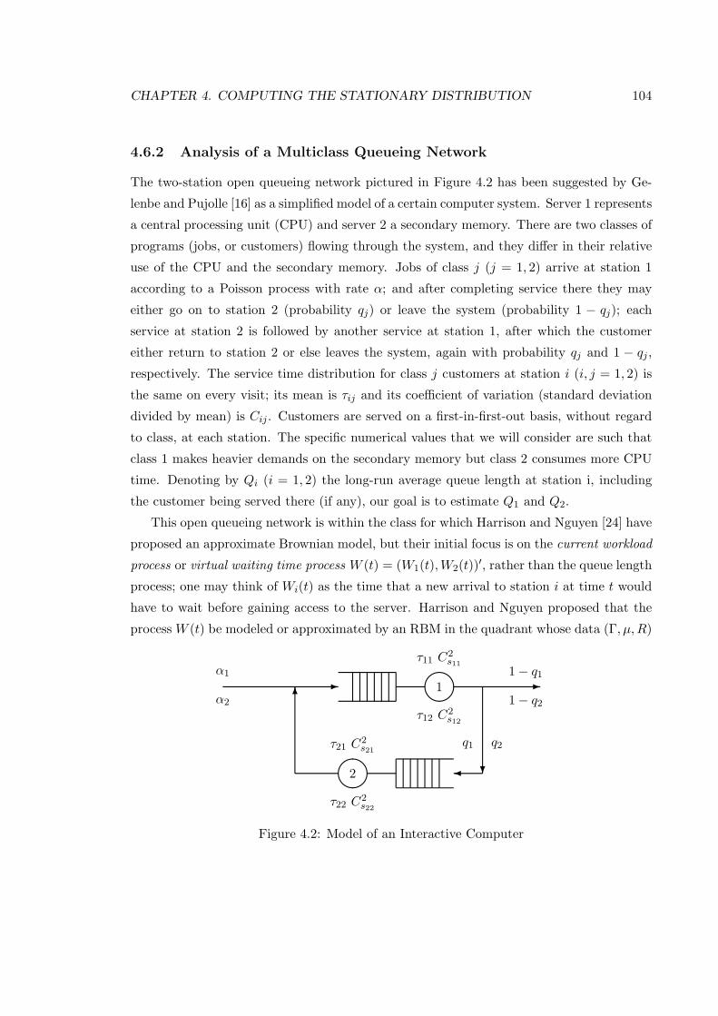
CHAPTER 4. COMPUTING THE STATIONARY DISTRIBUTION 104
4.6.2 Analysis of a Multiclass Queueing Network
The two-station open queueing network pictured in Figure 4.2 has been suggested by Ge-
lenbe and Pujolle [16] as a simplified model of a certain computer system. Server 1 represents
a central processing unit (CPU) and server 2 a secondary memory. There are two classes of
programs (jobs, or customers) flowing through the system, and they differ in their relative
use of the CPU and the secondary memory. Jobs of class j (j = 1, 2) arrive at station 1
according to a Poisson process with rate α; and after completing service there they may
either go on to station 2 (probability qj) or leave the system (probability 1 − qj); each
service at station 2 is followed by another service at station 1, after which the customer
either return to station 2 or else leaves the system, again with probability qj and 1 − qj ,respectively. The service time distribution for class j customers at station i (i, j = 1, 2) is
the same on every visit; its mean is τij and its coefficient of variation (standard deviation
divided by mean) is Cij . Customers are served on a first-in-first-out basis, without regard
to class, at each station. The specific numerical values that we will consider are such that
class 1 makes heavier demands on the secondary memory but class 2 consumes more CPU
time. Denoting by Qi (i = 1, 2) the long-run average queue length at station i, including
the customer being served there (if any), our goal is to estimate Q1 and Q2.
This open queueing network is within the class for which Harrison and Nguyen [24] have
proposed an approximate Brownian model, but their initial focus is on the current workload
process or virtual waiting time process W (t) = (W1(t),W2(t))′, rather than the queue length
process; one may think of Wi(t) as the time that a new arrival to station i at time t would
have to wait before gaining access to the server. Harrison and Nguyen proposed that the
process W (t) be modeled or approximated by an RBM in the quadrant whose data (Γ, µ,R)
α1-
α2
1
τ11 C2s11
τ12 C2s12
-1− q1
1− q2
?
q1 q2
τ21 C2s21
τ22 C2s22
2
6
Figure 4.2: Model of an Interactive Computer
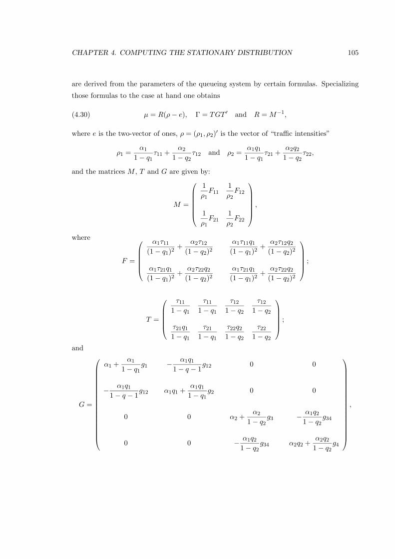
CHAPTER 4. COMPUTING THE STATIONARY DISTRIBUTION 105
are derived from the parameters of the queueing system by certain formulas. Specializing
those formulas to the case at hand one obtains
µ = R(ρ− e), Γ = TGT ′ and R = M−1,(4.30)
where e is the two-vector of ones, ρ = (ρ1, ρ2)′ is the vector of “traffic intensities”
ρ1 =α1
1− q1τ11 +
α2
1− q2τ12 and ρ2 =
α1q1
1− q1τ21 +
α2q2
1− q2τ22,
and the matrices M , T and G are given by:
M =
1ρ1F11
1ρ2F12
1ρ1F21
1ρ2F22
,
where
F =
α1τ11
(1− q1)2+
α2τ12
(1− q2)2
α1τ11q1
(1− q1)2+
α2τ12q2
(1− q2)2
α1τ21q1
(1− q1)2+
α2τ22q2
(1− q2)2
α1τ21q1
(1− q1)2+
α2τ22q2
(1− q2)2
;
T =
τ11
1− q1
τ11
1− q1
τ12
1− q2
τ12
1− q2
τ21q1
1− q1
τ21
1− q1
τ22q2
1− q2
τ22
1− q2
;
and
G =
α1 +α1
1− q1g1 − α1q1
1− q − 1g12 0 0
− α1q1
1− q − 1g12 α1q1 +
α1q1
1− q1g2 0 0
0 0 α2 +α2
1− q2g3 − α1q2
1− q2g34
0 0 − α1q2
1− q2g34 α2q2 +
α2q2
1− q2g4
,
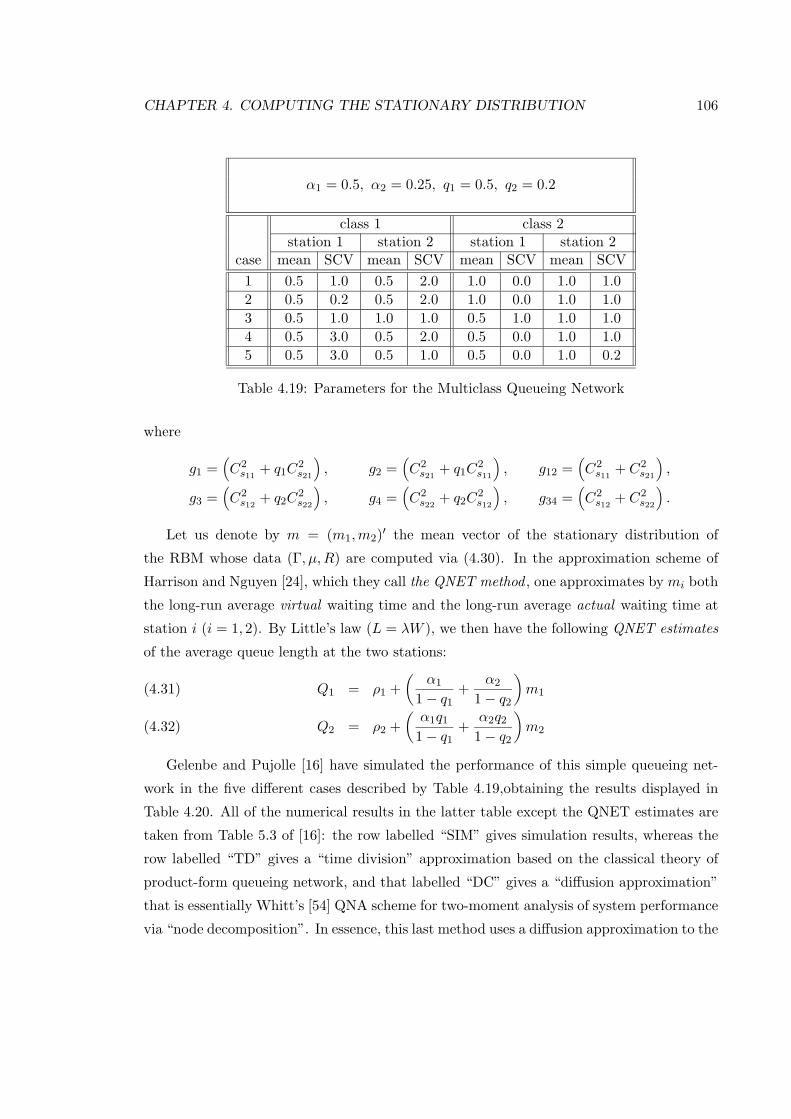
CHAPTER 4. COMPUTING THE STATIONARY DISTRIBUTION 106
α1 = 0.5, α2 = 0.25, q1 = 0.5, q2 = 0.2
class 1 class 2station 1 station 2 station 1 station 2
case mean SCV mean SCV mean SCV mean SCV1 0.5 1.0 0.5 2.0 1.0 0.0 1.0 1.02 0.5 0.2 0.5 2.0 1.0 0.0 1.0 1.03 0.5 1.0 1.0 1.0 0.5 1.0 1.0 1.04 0.5 3.0 0.5 2.0 0.5 0.0 1.0 1.05 0.5 3.0 0.5 1.0 0.5 0.0 1.0 0.2
Table 4.19: Parameters for the Multiclass Queueing Network
where
g1 =(C2s11
+ q1C2s21
), g2 =
(C2s21
+ q1C2s11
), g12 =
(C2s11
+ C2s21
),
g3 =(C2s12
+ q2C2s22
), g4 =
(C2s22
+ q2C2s12
), g34 =
(C2s12
+ C2s22
).
Let us denote by m = (m1,m2)′ the mean vector of the stationary distribution of
the RBM whose data (Γ, µ,R) are computed via (4.30). In the approximation scheme of
Harrison and Nguyen [24], which they call the QNET method , one approximates by mi both
the long-run average virtual waiting time and the long-run average actual waiting time at
station i (i = 1, 2). By Little’s law (L = λW ), we then have the following QNET estimates
of the average queue length at the two stations:
Q1 = ρ1 +(
α1
1− q1+
α2
1− q2
)m1(4.31)
Q2 = ρ2 +(α1q1
1− q1+
α2q2
1− q2
)m2(4.32)
Gelenbe and Pujolle [16] have simulated the performance of this simple queueing net-
work in the five different cases described by Table 4.19,obtaining the results displayed in
Table 4.20. All of the numerical results in the latter table except the QNET estimates are
taken from Table 5.3 of [16]: the row labelled “SIM” gives simulation results, whereas the
row labelled “TD” gives a “time division” approximation based on the classical theory of
product-form queueing network, and that labelled “DC” gives a “diffusion approximation”
that is essentially Whitt’s [54] QNA scheme for two-moment analysis of system performance
via “node decomposition”. In essence, this last method uses a diffusion approximation to the
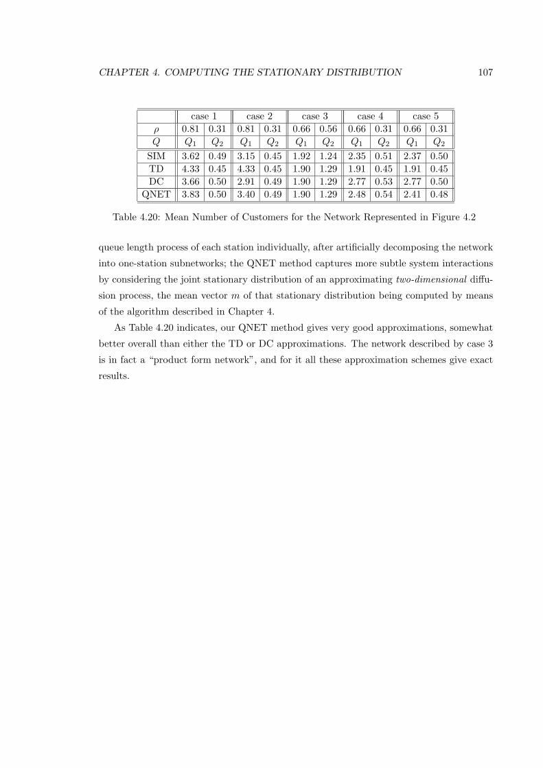
CHAPTER 4. COMPUTING THE STATIONARY DISTRIBUTION 107
case 1 case 2 case 3 case 4 case 5ρ 0.81 0.31 0.81 0.31 0.66 0.56 0.66 0.31 0.66 0.31Q Q1 Q2 Q1 Q2 Q1 Q2 Q1 Q2 Q1 Q2
SIM 3.62 0.49 3.15 0.45 1.92 1.24 2.35 0.51 2.37 0.50TD 4.33 0.45 4.33 0.45 1.90 1.29 1.91 0.45 1.91 0.45DC 3.66 0.50 2.91 0.49 1.90 1.29 2.77 0.53 2.77 0.50
QNET 3.83 0.50 3.40 0.49 1.90 1.29 2.48 0.54 2.41 0.48
Table 4.20: Mean Number of Customers for the Network Represented in Figure 4.2
queue length process of each station individually, after artificially decomposing the network
into one-station subnetworks; the QNET method captures more subtle system interactions
by considering the joint stationary distribution of an approximating two-dimensional diffu-
sion process, the mean vector m of that stationary distribution being computed by means
of the algorithm described in Chapter 4.
As Table 4.20 indicates, our QNET method gives very good approximations, somewhat
better overall than either the TD or DC approximations. The network described by case 3
is in fact a “product form network”, and for it all these approximation schemes give exact
results.
Appendix A
Detailed Description of the
Algorithm
In this appendix, we will give a detailed description of one version of the general algorithm
described in Chapter 4. This version has been implemented in a software package, called
BNET, to calculate the stationary density of a semimartingale Reflected Brownian motion
(SRBM) in an orthant Rd+. BNET will be the kernel of a larger software package, tentatively
called QNET, that can be used for performance analysis for a wide class of queueing network
models. This implementation of BNET is by no means “optimal”. However, the numerical
results in Sections 4.5–4.6 show that it performs quite well.
The actual code of BNET for this implementation is in “C”. In the first four sections,
we will give a description of the algorithm that is independent of any particular language,
and in Section 5 we will give the “C” code for most essential functions (routines) in BNET.
A.1 Input Parameters and Scaling
Inputs
The input parameters to BNET are (d,Γ, µ,R, n), where
a) d is a positive integer. It is the dimension of the state space of an SRBM;
b) Γ is a d× d positive definite matrix. It is the covariance matrix of an SRBM;
c) µ is a d-dimensional vector. It is the drift vector of an SRBM;
108
APPENDIX A. DETAILED DESCRIPTION OF THE ALGORITHM 109
d) R is a d× d matrix with diag(R) > 0. It is the reflection matrix of an SRBM;
e) n is a positive integer. It is the maximum degree of polynomials that we used in (4.23).
In input mode, BNET will exit immediately and send a corresponding error message to a
user, if one of the following happens:
i) d or n is not a positive integer;
ii) Γ is not symmetric or not positive definite;
iii) diag(R) 6> 0, SRBM does not exist;
iv) R is not invertible, stationary distribution does not exist;
v) R−1µ 6< 0, stationary distribution does not exist.
Scaling
After all the input parameters have passed the five tests above, we then scale parameters
(Γ, µ,R) as follows.
Γ∗ij =Γij√
Γii√
Γjj, R∗ij =
RijRjj
√Γjj√Γii
, µ∗i =µi√
Γiiγmax,
where γmax is the largest component of
γ ≡ −R∗−1
µ1/√
Γ11
...
µd/√
Γdd
> 0.
The idea of the scaling above is to obtain a (Γ∗, µ∗, R∗)-SRBM with Γ∗ii = 1, R∗ii = 1 and
max1≤i≤d γ∗i = 1, where
γ∗ ≡ −R∗−1µ∗ =γ
γmax.
We believe that using this normalized set of data (Γ∗, µ∗, R∗) will make BNET more robust.
The logic of the scaling was explained in Proposition 4.4. Suppose that m∗ is the steady-
state mean of a (Γ∗, µ∗, R∗)-SRBM. Then we have the steady state mean m = (m1, . . . ,md)′
of the SRBM Z given by
mi =√
Γiiγmax
m∗i , i = 1, 2, . . . , d.(A.1)
APPENDIX A. DETAILED DESCRIPTION OF THE ALGORITHM 110
The memory spaces of (Γ, µ,R) can be used to store the converted data (Γ∗, µ∗, R∗).
The spaces of off-diagonal elements of Γ can be used to store the corresponding element of
Γ∗. Since the diagonal elements of Γ∗ are one, the spaces of diagonal elements of Γ still
keep old values, i.e., Γii’s. The old Γii values are needed in (A.1). Similarly, the spaces of
µ and R can be used to store the corresponding element of µ∗ and R∗. In the mean time,
we need additional spaces to keep the constant γmax, which is needed in (A.1).
From now on, (d,Γ, µ,R, n, γmax) refers to converted data (with the asterisk omitted),
instead of original input data. Notice that γmax and the diagonal elements of Γ are not
accessed until the final output routine, see (A.1).
A.2 Indexing
In light of the definition of Hn in (4.23), we need a systematic and efficient way to enumerate
the elements of the following family of functions:xi11 x
i22 · · ·x
idd : 0 < i1 + i2 + · · ·+ id ≤ n, ij ’s are non-negative integers
.
It is equivalent to enumerate the elements of following subset of Zd+:
I(d, n) ≡ (i1, i2, . . . , id) : i1 + i2 + · · ·+ id ≤ n, ij ’s are non-negative integers .
First, we have #I(d, n) = Cdn+d ≡ (d+1)(d+2) · · · (d+n)/n!. To see this, suppose that there
are n balls and d vertical bars. Mix these d+n objects, and arrange them on a straight line.
For each such arrangement, let i1 be the number of balls to the left of the first bar, and i2
be the number of balls between the first bar and the second bar. Similarly we can define i3,
. . ., id. Obviously, such an (i1, . . . , id) ∈ I(d, n), and each arrangement corresponds exactly
one element in I(d, n). The total number of such arrangements is Cdd+n (Balls and bars are
assumed to be indistinguishable). Therefore, we have shown #I(d, n) = Cdd+n. Since the
dimensions of these sets I are used frequently, we can pre-compute them and store them in
a d× (n+ 1) matrix C, i.e.,
Clk ≡ #I(l, k) = C ll+k =(l + 1)(l + 2) · · · (l + k)
k!, 1 ≤ l ≤ d, 0 ≤ k ≤ n.
Now for an I = (i1, i2, . . . , id) ∈ I(d, n), we are going to map it into an integer, denoted
as Index(d, I), between 1 and Cdn. In the future, we are going to access this I through the
APPENDIX A. DETAILED DESCRIPTION OF THE ALGORITHM 111
integer. The function Index() is defined as follows:
Index(d, I) ≡ #I(d, i1 + i2 + · · ·+ id − 1) +(A.2)
+ #I(d− 1, i2 + · · ·+ id − 1) + · · ·+
+ #I(1, id − 1) + 1.
From this definition, we have Index(d, (0, . . . , 0)) = 1 and Index(d, (0, . . . , 0, n)) = Cdn.
Conversely, given an 1 ≤ i ≤ Cdn, we need to find the unique I = (i1, i2, . . . , id) ∈ I(d, n)
so that i = Index(d, I). Such an I is going to be denoted as InverseIndex(d, i), or simply
Ii. We are going to add one more component for Ii, i.e.,
Ii = (i0, i1, . . . , id), with i0 = i1 + . . .+ id.
Keeping track of i0 sometimes makes our description easier as we will see shortly. Let kdbe the smallest k such that
#I(d, k − 1) < i ≤ #I(d, k),
and kd−1 be the smallest k such that
#I(d− 1, k − 1) < i−#I(d, kd − 1) ≤ #I(d− 1, k).
Inductively, we can define kd−2, . . ., and k1, where k1 is the smallest k such that
#I(1, k− 1) < i−#I(d, kd − 1)−#I(d− 1, kd−1 − 1) + . . .+ #I(2, k2 − 1) ≤ #I(d− 1, k).
We can use either linear search or binary search to locate above k. Having found (kd, kd−1,
. . ., k1), we define
i0 = kd, i1 = kd − kd−1, i2 = kd−1 − kd−2
...
id−1 = k2 − k1, id = k1.
Then I = (i0, i1, . . . , id) has the desired property. Again, like C’s, these I’s can be pre-
computed and stored in a Cdn × (d+ 1) matrix I, i.e., for i = 1, . . . , Cdn,
Ii = (Ii0, Ii1, . . . , Iid).
APPENDIX A. DETAILED DESCRIPTION OF THE ALGORITHM 112
A.3 Basis and Inner Product
Natural Basis of Hn
Now we are able to enumerate the polynomials in Hn as Af2, . . ., AfCnd . The typical
element of fi’s looks like
fi(x1, x2, . . . , xd) = xIi11 xIi22 · · ·xIidd .
For 2 ≤ i ≤ Cdn, the first step is to store Afi. It has two parts, interior part which is equal
to Gfi and boundary part which is equal to (D1fi, . . . , Ddfi). Function Gfi is a polynomial
of degree Ii0 − 1 with d variables and Dlfi is a polynomial of degree Ii0 − 1 with d − 1
variable (l = 1, . . . , d). Following the enumeration scheme in the previous section, only the
coefficients of these polynomials need to be stored. For each i, we enumerate the coefficients
of Gfi from 1, . . . , Cd(Ii0−1). For j = 1, 2, . . . , d,
a. if Iij ≥ 1,
Gfi(Ii1, . . . , Ii(j−1), Iij − 1, Ii(j+1), . . . , Iid) ≡ Iijµj ;
b. if Iij ≥ 2, because Γjj = 1,
Gfi(Ii1, . . . , Ii(j−1), Iij − 2, Ii(j+1), . . . , Iid) ≡12Iij(Iij − 1);
c. if Iij ≥ 1 & Iik ≥ 1, k = j + 1, . . . , d,
Gfi(Ii1, . . . , , Iij − 1, . . . , Iik − 1, . . . , Iid) ≡ IijIikΓjk;
d. for all the other cases of (i1, . . . , id) with i1 + · · ·+ id ≤ Ii0 − 1,
Gfi(i1, · · · , id) = 0.
Similarly, for l = 1, 2, . . . , d, we enumerate the coefficients of Dlfi from 1, . . . , C(d−1)(Ii0−1).
Dlfi has only d− 1 variable because xl = 0. For j = 1, 2, . . . , d,
e. if Iil = 1,
Dlfi(Ii1, . . . , Iil, Iid) ≡ Rll;
f. if Iil = 0 & Iij ≥ 1,
DlfI(Ii1, . . . , Iij − 1, . . . , Iil, . . . , Iid) ≡ IijRjl;
APPENDIX A. DETAILED DESCRIPTION OF THE ALGORITHM 113
g. all the other cases
Dlfi(i1, . . . , il, . . . , id) = 0,
where il means this component is missing in a vector. Therefore we can store Afi in a
sequence of records
Afi =
Afi ·itr = Gfi
Afi ·bd[1 . . . d] = (D1fi, . . . , Ddfi),i = 2, 3, . . . , Cdn,
(Af1 = 0 and is omitted).
Inner product
Let f = (f · itr, f · bd1, . . . , f · bdd) be a polynomial of degree k, i.e., f · itr is a d variable
polynomial of degree k and f · bdl is a d − 1 variable polynomial of degree k. Let g =
(g · itr, g ·bd1, . . . , g ·bdd) be another polynomial of degree m, the inner product 〈f, k, g,m〉between f and g is defined as
〈f, k, g,m〉 ≡∫S
(f ·itr)(g ·itr) exp(−2γ ·x) dx+12
d∑l=1
∫Fl
(f ·bdl)(g ·bdl) exp(−2γ ·x) dσl
=∑
i1+...+id≤k
∑j1+...+jd≤m
(f ·itr)(i1, i2, . . . , id)(g ·itr)(j1, j2, . . . , jd)×
× (i1 + j1)!(2γ1)i1+j1+1
× · · · × (id + jd)!(2γd)id+jd+1
+12
d∑l=1
∑i1+...+il+...id≤k
∑j1+...+jl+...jd≤m
(f ·bdl)(i1, . . . , il, . . . id)×
× (g ·bdl)(j1, . . . , jl, . . . , jd)(i1 + j1)!
(2γ1)i1+j1+1× · · · l term · · · × (id + jd)!
(2γd)id+jd+1.
Because this inner product function is used frequently in BNET, reducing its run time will
significantly improve the efficiency of BNET. Function call to calculate weighting factor
(il + jl)/(2γl)i1+j1+1 is expensive. Therefore we can also pre-compute them and store them
as w, i.e.,
w[l][i] ≡ i!(2γl)i+1
, 1 ≤ l ≤ d, 0 ≤ i ≤ 2n.
A.4 Stationary Density
There are several ways to find rn defined in Proposition 4.3. In this section, we present two
ways to do it. One is to use orthogonalization, the other is to solve a linear equation.
APPENDIX A. DETAILED DESCRIPTION OF THE ALGORITHM 114
Orthogonalizing Basis Elements
Let ψ2 = Af2, and for i = 3, . . . , Cdn, let
ψi ≡ Afi −i−1∑k=2
〈Afi, ψk〉〈ψk, ψk〉
ψk.
Then ψ2, ψ3, . . . , ψCdn is an orthogonal basis of Hn. Let
ψ1 = (1, 1, . . . , 1) and φ0 = (1, 0, . . . , 0).
Then the orthogonal complement φn (see Proposition 4.3) of ψ1 onto Hn is given by
φn ≡ ψ1 −Cdn∑k=2
〈ψk, ψ1〉〈ψk, ψk〉
ψk.
Hence
rn ≡φn
〈φn, φ0〉.
Letting
pn = rn exp(−2γ ·x),
we have ∫S
(pn ·itr) dx = 1, mj.=∫S
(xi pn ·itr) dx = 〈xi, rn〉,
where xi is the polynomial (xi, 0, . . . , 0).
Solving Linear Equation
The orthogonal complement φn of ψ1 on to Hn is equal to
φn = ψ1 − ψ1,
where ψ1 is the projection of ψ1 on to Hn. Because Afi, 2 ≤ i ≤ Cdn is a basis for Hn,
there exist constants a2, . . . , aCdn such that
ψ1 =Cdn∑i=2
aiAfi.
Therefore
φn = ψ1 −Cdn∑i=2
aiAfi.
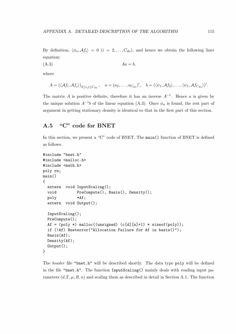
APPENDIX A. DETAILED DESCRIPTION OF THE ALGORITHM 115
By definition, 〈φn,Afi〉 = 0 (i = 2, . . . , Cdn), and hence we obtain the following liner
equation:
Aa = b,(A.3)
where
A = (〈Afi,Afj〉)2≤i,j≤Cdn , a = (a2, . . . , aCdn)′, b = (〈ψ1,Af2〉, . . . , 〈ψ1,AfCdn〉)′.
The matrix A is positive definite, therefore it has an inverse A−1. Hence a is given by
the unique solution A−1b of the linear equation (A.3). Once φn is found, the rest part of
argument in getting stationary density is identical to that in the first part of this section.
A.5 “C” code for BNET
In this section, we present a “C” code of BNET. The main() function of BNET is defined
as follows.
#include "bnet.h"#include <malloc.h>#include <math.h>poly rn;main()
extern void InputScaling();void PreCompute(), Basis(), Density();poly *Af;extern void Output();
InputScaling();PreCompute();Af = (poly *) malloc((unsigned) (c[d][n]+1) * sizeof(poly));if (!Af) Bneterror("Allocation Failure for Af in basis()");Basis(Af);Density(Af);Output();
The header file "bnet.h" will be described shortly. The data type poly will be defined
in the file "bnet.h". The function InputScaling() mainly deals with reading input pa-
rameters (d,Γ, µ,R, n) and scaling them as described in detail in Section A.1. The function
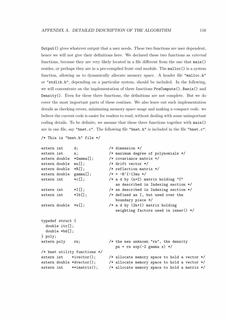
APPENDIX A. DETAILED DESCRIPTION OF THE ALGORITHM 116
Output() gives whatever output that a user needs. These two functions are user dependent,
hence we will not give their definitions here. We declared these two functions as external
functions, because they are very likely located in a file different from the one that main()
resides, or perhaps they are in a pre-compiled front–end module. The malloc() is a system
function, allowing us to dynamically allocate memory space. A header file "malloc.h"
or "stdlib.h", depending on a particular system, should be included. In the following,
we will concentrate on the implementation of three functions PreCompute(), Basis() and
Density(). Even for these three functions, the definitions are not complete. But we do
cover the most important parts of these routines. We also leave out such implementation
details as checking errors, minimizing memory space usage and making a compact code. we
believe the current code is easier for readers to read, without dealing with some unimportant
coding details. To be definite, we assume that these three functions together with main()
are in one file, say "bnet.c". The following file "bnet.h" is included in the file "bnet.c".
/* This is "bnet.h" file */
extern int d; /* dimension */extern int n; /* maximum degree of polynomials */extern double *Gamma[]; /* covariance matrix */extern double mu[]; /* drift vector */extern double *R[]; /* reflection matrix */extern double gamma[]; /* = -R^-1mu */extern int *c[]; /* a d by (n+2) matrix holding "C"
as described in Indexing section */extern int *I[]; /* as described in Indexing section */extern int *Ib[]; /* defined as I, but used over the
boundary piece */extern double *w[]; /* a d by (2n+1) matrix holding
weighting factors used in inner() */
typedef struct double itr[];double *bd[];
poly;extern poly rn; /* the new unknown "rn", the density
pn = rn exp(-2 gamma x) *//* bnet utility functions */extern int *ivector(); /* allocate memory space to hold a vector */extern double *dvector(); /* allocate memory space to hold a vector */extern int **imatrix(); /* allocate memory space to hold a matrix */
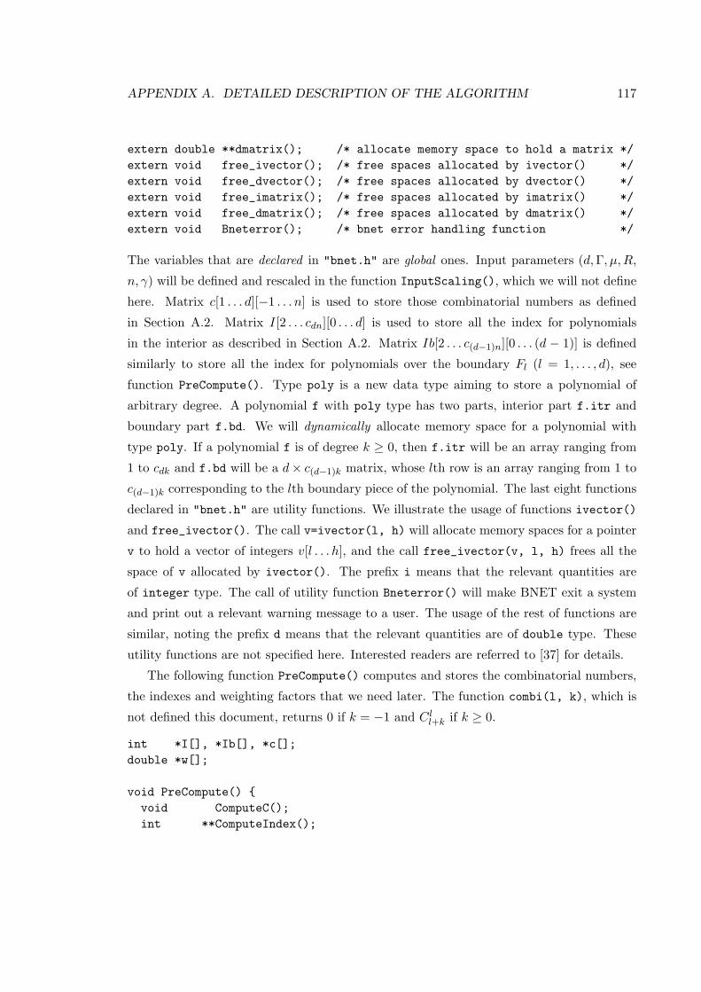
APPENDIX A. DETAILED DESCRIPTION OF THE ALGORITHM 117
extern double **dmatrix(); /* allocate memory space to hold a matrix */extern void free_ivector(); /* free spaces allocated by ivector() */extern void free_dvector(); /* free spaces allocated by dvector() */extern void free_imatrix(); /* free spaces allocated by imatrix() */extern void free_dmatrix(); /* free spaces allocated by dmatrix() */extern void Bneterror(); /* bnet error handling function */
The variables that are declared in "bnet.h" are global ones. Input parameters (d,Γ, µ,R,
n, γ) will be defined and rescaled in the function InputScaling(), which we will not define
here. Matrix c[1 . . . d][−1 . . . n] is used to store those combinatorial numbers as defined
in Section A.2. Matrix I[2 . . . cdn][0 . . . d] is used to store all the index for polynomials
in the interior as described in Section A.2. Matrix Ib[2 . . . c(d−1)n][0 . . . (d − 1)] is defined
similarly to store all the index for polynomials over the boundary Fl (l = 1, . . . , d), see
function PreCompute(). Type poly is a new data type aiming to store a polynomial of
arbitrary degree. A polynomial f with poly type has two parts, interior part f.itr and
boundary part f.bd. We will dynamically allocate memory space for a polynomial with
type poly. If a polynomial f is of degree k ≥ 0, then f.itr will be an array ranging from
1 to cdk and f.bd will be a d× c(d−1)k matrix, whose lth row is an array ranging from 1 to
c(d−1)k corresponding to the lth boundary piece of the polynomial. The last eight functions
declared in "bnet.h" are utility functions. We illustrate the usage of functions ivector()
and free_ivector(). The call v=ivector(l, h) will allocate memory spaces for a pointer
v to hold a vector of integers v[l . . . h], and the call free_ivector(v, l, h) frees all the
space of v allocated by ivector(). The prefix i means that the relevant quantities are
of integer type. The call of utility function Bneterror() will make BNET exit a system
and print out a relevant warning message to a user. The usage of the rest of functions are
similar, noting the prefix d means that the relevant quantities are of double type. These
utility functions are not specified here. Interested readers are referred to [37] for details.
The following function PreCompute() computes and stores the combinatorial numbers,
the indexes and weighting factors that we need later. The function combi(l, k), which is
not defined this document, returns 0 if k = −1 and C ll+k if k ≥ 0.
int *I[], *Ib[], *c[];double *w[];
void PreCompute() void ComputeC();int **ComputeIndex();
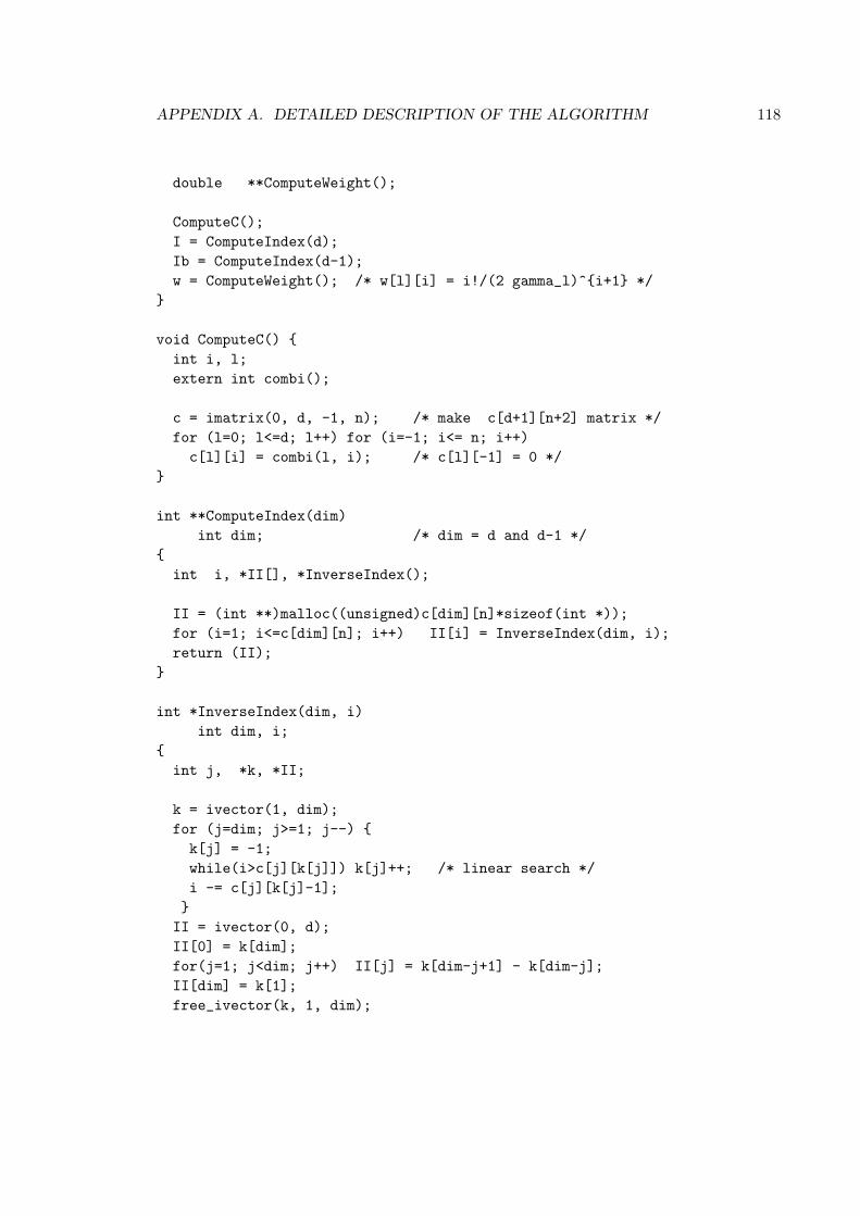
APPENDIX A. DETAILED DESCRIPTION OF THE ALGORITHM 118
double **ComputeWeight();
ComputeC();I = ComputeIndex(d);Ib = ComputeIndex(d-1);w = ComputeWeight(); /* w[l][i] = i!/(2 gamma_l)^i+1 */
void ComputeC() int i, l;extern int combi();
c = imatrix(0, d, -1, n); /* make c[d+1][n+2] matrix */for (l=0; l<=d; l++) for (i=-1; i<= n; i++)c[l][i] = combi(l, i); /* c[l][-1] = 0 */
int **ComputeIndex(dim)int dim; /* dim = d and d-1 */
int i, *II[], *InverseIndex();
II = (int **)malloc((unsigned)c[dim][n]*sizeof(int *));for (i=1; i<=c[dim][n]; i++) II[i] = InverseIndex(dim, i);return (II);
int *InverseIndex(dim, i)int dim, i;
int j, *k, *II;
k = ivector(1, dim);for (j=dim; j>=1; j--) k[j] = -1;while(i>c[j][k[j]]) k[j]++; /* linear search */i -= c[j][k[j]-1];II = ivector(0, d);II[0] = k[dim];for(j=1; j<dim; j++) II[j] = k[dim-j+1] - k[dim-j];II[dim] = k[1];free_ivector(k, 1, dim);
APPENDIX A. DETAILED DESCRIPTION OF THE ALGORITHM 119
return (II);
void ComputeWeight()
int i, l;/* extern double pow() is a math library function */long factorial();int twon;
twon = 2 * n;w = dmatrix(1, d, 0, twon);for (l=1; l<=d ; l++) for (i=0; i<= twon; i++)w[l][i] = factorial(i)/pow(2*gamma[l], (double) i+1);
In the following routine Basis(), we find the natural basis Af2, . . . ,Afcdn . Readers can
refer to Section A.3 for more details. Function Index() is straightforwardly implemented
according to the description in Section A.2. Function initpoly() is nothing but allocate
enough space to hold a ith degree polynomial and initialize to be zero.
void Basis(Af)poly *Af;
int i, j, l, k;int *II, *IIb;poly initpoly();long Index();
II = ivector(0, d);IIb= ivector(0, d-1);for (i=2; i<=c[d][n]; i++)
initpoly(A+i, I[i][0]-1);/* starts filling interior polynomial */for (j=0; j<=d; j++) II[j] = I[i][j];for (j=1; j<=d; j++)
if (II[j]>=1) II[0]--; II[j]--;Af[i].itr[Index(d, II)]=I[i][j]*mu[j];if (II[j]>=1)
II[0]--; II[j]--;Af[i].itr[Index(d,II)] = I[i][j]*(I[i][j]-1)/2;
APPENDIX A. DETAILED DESCRIPTION OF THE ALGORITHM 120
II[0]++; II[j]++;II[0]++; II[j]++;
for (j=1; j<=d; j++) for (l=j+1; l<=d; l++)
if (II[j] >=1 && II[l] >=1) II[0] -= 2; II[j]--; II[l]--;Af[i].itr[Index(d, II)] = I[i][j] * I[i][l] * Gamma[j][l];II[0] += 2; II[j]++; II[l]++;
/* starts filling boundary polynomials */for (j=1; j<=d; j++)
if (II[j] == 1) IIb[0] = II[0] - 1;for (l=1; l<j; l++) IIb[l] = II[l];for (l=j; l<d; l++) IIb[l] = II[l+1];Af[i].bd[j][Index(d-1, IIb)] = R[j][j];
if (II[j] == 0) for (l=1; l<=d; l++) if (II[l] >= 1)
II[l]--;for (k=0; k<j; k++) IIb[k] = II[k];for (k=j; k<d; k++) IIb[k] = II[k+1];IIb[0]--; II[l]++;Af[i].bd[j][Index(d-1, IIb)] = II[l] * R[l][j];
free_ivector(II, 0, d);free_ivector(IIb, 0, d-1);
void initpoly(f, k)poly *f;int k;
int l, i;
f->itr = dvector(1, c[d][k]);for (i=1; i<=c[d][k]; i++)(f->itr)[i] = 0.0;
APPENDIX A. DETAILED DESCRIPTION OF THE ALGORITHM 121
f->bd = dmatrix(1, d, 1, c[d-1][k]);for (l=1; l<=d; l++)for (i=1; i<=c[d-1][k]; i++)
(f->bd)[l][i] = 0.0;
long Index(dim, II)int dim, *II;
long tmp=1;int l, k=II[0]-1;
for (l=dim; l>=1; l--) tmp += c[l][k];k -= II[dim-l+1];
return (tmp);
Our next task is to define the function Density() to find the weighted density function
rn. In the definition, we need to calculate the inner product of two polynomials. Suppose
that f and g are two polynomials with type poly of degree k and m, respectively. Then
function inner(f, t, g, m) should return the inner product of f and g. It is implemented
according the formula given in the “Inner Product” section. We comment that in calculat-
ing a term like (i1 + j1)!/(2γ1)i1+j1+1, one would like to use those pre-compute weighted
factors w[l][i]. Apparently, storage for these quantities is not a problem, however, it saves
tremendous number of functions calls to calculate (i1 + j1)! and (2γ1)i1+j1+1 in real time.
The function half_linear(f, t, a, g, m, h) performs h = f + ag with m ≤ t, where
f and g are polynomials of degree k and m, respectively, and a is a real number.
void Density(Af)poly *Af;
int i, j, l, k;poly phi_0;double tmp;extern double inner();extern void half_linear();extern void initpoly();
APPENDIX A. DETAILED DESCRIPTION OF THE ALGORITHM 122
extern void orthogonalize();
/* give space and initialize */initpoly(&rn, n-1);initpoly(&phi_0, 0);phi_0.itr[1] = 1.0; /*phi_0 = (1; 0, 0, ..., 0) */rn.itr[1] = 1.0; /*p = psi_1=(1; 1, 1, ..., 1) */for (l=1; l<=d; l++) rn.bd[l][1] = 1.0;phi_0.bd[l][1] = 1.0;
/* set phi_0 = phi_1 *//* end of initialization */
orthogonalize(Af);for ( k=2; k<=c[d][n]; k++) tmp = inner(Af[k], I[k][0]-1, Af[k], I[k][0]-1);if ( tmp ==0.0)
Bneterror(" Can not be normalized when finding density");tmp = - inner(phi_0, 0 , Af[k], I[k][0]-1)/tmp;half_linear( rn, n-1, tmp, Af[k], I[k][0]-1, &rn);
/* normalize */for (l=1; l<=d; l++) /* set phi_0 back to phi_0 */phi_0.bd[l][1] = 0.0;
tmp = inner( phi_0, 0, rn, n-1);if ( tmp==0.0) Bneterror(" can not be noramlized into a density");tmp = 1/tmp;for ( i=1; i<=c[d][n-1]; i++)rn.itr[i] *= tmp;
for ( j =1; j<=d; j++)for ( i=1; i<=c[d-1][n-1]; i++)
rn.bd[j][i] *= tmp;
void orthogonalize(Af)poly *Af;
int t, i;double tmp;extern double inner();extern void half_linear();extern void Bneterror();
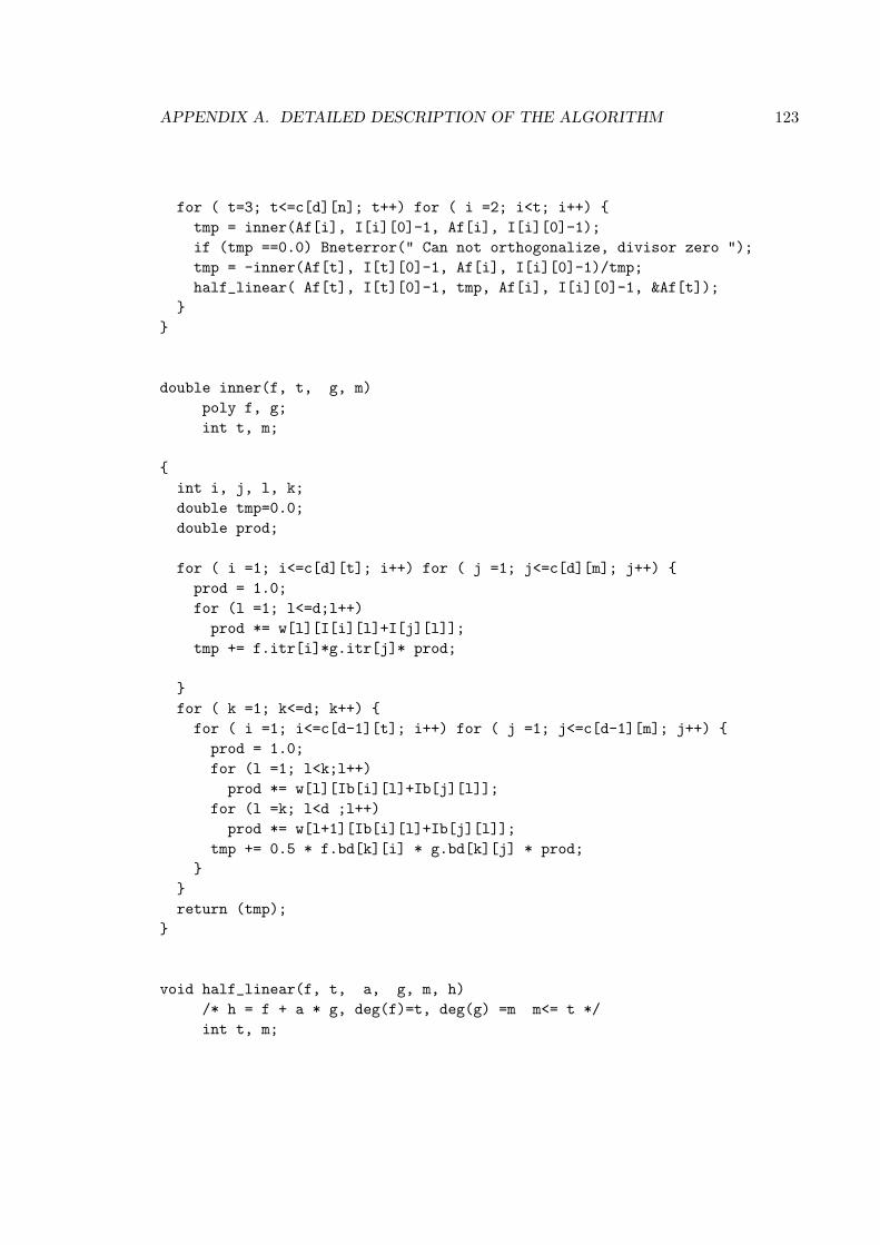
APPENDIX A. DETAILED DESCRIPTION OF THE ALGORITHM 123
for ( t=3; t<=c[d][n]; t++) for ( i =2; i<t; i++) tmp = inner(Af[i], I[i][0]-1, Af[i], I[i][0]-1);if (tmp ==0.0) Bneterror(" Can not orthogonalize, divisor zero ");tmp = -inner(Af[t], I[t][0]-1, Af[i], I[i][0]-1)/tmp;half_linear( Af[t], I[t][0]-1, tmp, Af[i], I[i][0]-1, &Af[t]);
double inner(f, t, g, m)poly f, g;int t, m;
int i, j, l, k;double tmp=0.0;double prod;
for ( i =1; i<=c[d][t]; i++) for ( j =1; j<=c[d][m]; j++) prod = 1.0;for (l =1; l<=d;l++)
prod *= w[l][I[i][l]+I[j][l]];tmp += f.itr[i]*g.itr[j]* prod;
for ( k =1; k<=d; k++) for ( i =1; i<=c[d-1][t]; i++) for ( j =1; j<=c[d-1][m]; j++)
prod = 1.0;for (l =1; l<k;l++)
prod *= w[l][Ib[i][l]+Ib[j][l]];for (l =k; l<d ;l++)
prod *= w[l+1][Ib[i][l]+Ib[j][l]];tmp += 0.5 * f.bd[k][i] * g.bd[k][j] * prod;
return (tmp);
void half_linear(f, t, a, g, m, h)/* h = f + a * g, deg(f)=t, deg(g) =m m<= t */int t, m;
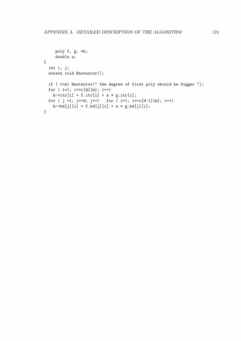
APPENDIX A. DETAILED DESCRIPTION OF THE ALGORITHM 124
poly f, g, *h;double a;
int i, j;extern void Bneterror();
if ( t<m) Bneterror(" the degree of first poly should be bigger ");for ( i=1; i<=c[d][m]; i++)
h->itr[i] = f.itr[i] + a * g.itr[i];for ( j =1; j<=d; j++) for ( i=1; i<=c[d-1][m]; i++)
h->bd[j][i] = f.bd[j][i] + a * g.bd[j][i];
Bibliography
[1] M. Berman and M. Westcott. On queueing systems with renewal departure processes.
Adv. Appl. Prob., 15:657–673, 1983.
[2] A. Bernard and A. El Kharroubi. Regulations de processus dans le premier “orthant”
de Rn. Stochastics, to appear.
[3] P. Billingsley. Convergence of Probability Measures. Wiley, New York, 1968.
[4] P. Billingsley. Probability and Measure. Wiley, 2nd edition, 1986.
[5] J. Bramble and A. Schatz. Rayleigh–Ritz–Galerkin methods for Dirichlet’s problem
using subspaces without boundary conditions. Comm. Pure Appl. Math., 23:653–675,
1970.
[6] K. L. Chung and R. J. Williams. Introduction to Stochastic Integration. Birkhauser,
Boston, 2nd edition, 1990.
[7] E. G. Coffman and M. I. Reiman. Diffusion approximations for computer/comunica-
tion systems. In G. Iazeolla, P. J. Courtois, and A. Hordijk, editors, Mathematical
Computer Performance and Reliability, Amsterdam, 1984. North-Holland.
[8] J. G. Dai. The existence of invariant probability measures for a class of Feller processes.
Journal of Nanjing University: Natural Science Edition, 21:245–252, 1985. (in Chinese
with English abstract).
[9] J. G. Dai and J. M. Harrison. Steady-state analysis of RBM in a rectangle: numerical
methods and a queueing application. Annals of Applied Probability, to appear in 1991.
[10] P. E. Echeverria. A criterion for invariant measures of Markov processes. Z. Wahrsch.
verw. Gebiete, 61:1–16, 1982.
125
BIBLIOGRAPHY 126
[11] S. N. Ethier and T. G. Kurtz. Markov Processes: Characterization and Convergence.
Wiley, New York, 1986.
[12] C. Flores. Diffusion approximations for computer communications networks. In
B. Gopinath, editor, Computer Communications, Proc. Symp. Appl. Math., Provi-
dence, R. I., 1985. Amer. Math. Soc.
[13] M. Foddy. Analysis of Brownian motion with drift, confined to a quadrant by oblique
reflection. PhD thesis, Department of Mathematics, Stanford University, 1983.
[14] G. J. Foschini. Equilibria for diffusion models of pairs of communicating computers–
symmetric case. IEEE Trans. Inform. Theory, 28:273–284, 1982.
[15] J. R. Fraker. Approximate techniques for the analysis of tandem queueing systems.
PhD thesis, Department of Industrial Engineering, Clemson University, 1971.
[16] E. Gelenbe and G. Pujolle. Introduction to Queueing Networks. Wiley, New York,
1987.
[17] D. Gilbard and N. S. Trudinger. Elliptic Partial Differential Equations of Second Order.
Springer-Verlag, New York, 2nd edition, 1983.
[18] P. W. Glynn. Diffusion approximations. Technical Report 38, Department of Opera-
tions Research, Stanford University, 1989.
[19] B. S. Greenberg. Queueing systems with returning customers and the order of tandem
queues. PhD thesis, University of California, Berkeley, 1986.
[20] B. S. Greenberg and R. W. Wolff. Optimal order of servers for tandem queues in light
traffic. Management Science, 34:500–508, 1988.
[21] J. M. Harrison. The heavy traffic approximation for single server queues in series. J.
Appl. Prob., 10:613–629, 1973.
[22] J. M. Harrison. The diffusion approximation for tandem queues in heavy traffic. Adv.
Appl. Prob., 10:886–905, 1978.
[23] J. M. Harrison, H. Landau, and L. A. Shepp. The stationary distribution of reflected
Brownian motion in a planar region. Annals of Probability, 13:744–757, 1985.
BIBLIOGRAPHY 127
[24] J. M. Harrison and V. Nguyen. The QNET method for two-moment analysis of open
queueing networks. Queueing Systems: Theory and Applications, 6:1–32, 1990.
[25] J. M. Harrison and M. I. Reiman. Reflected Brownian motion on an orthant. Annals
of Probability, 9:302–308, 1981.
[26] J. M. Harrison and R. J. Williams. Brownian models of open queueing networks with
homogeneous customer populations. Stochastics, 22:77–115, 1987.
[27] J. M. Harrison and R. J. Williams. Multidimensional reflected Brownian motions
having exponential stationary distributions. Annals of Probability, 15:115–137, 1987.
[28] J. M. Harrison, R. J. Williams, and H. Chen. Brownian models of closed queueing
networks with homogeneous customer populations. Stochastics, 29:37–74, 1990.
[29] N. Ikeda and S. Watanabe. Stochastic Differential Equations and Diffusion Processes.
North-Holland, New York, 1981.
[30] T. G. Kurtz. Random time change and convergence in distribution. to appear.
[31] T. G. Kurtz. A control formulation for constrained Markov processes. In Proceedings
of the AMS-SIAM Summer Seminar on Mathematics of Random Media, Blacksburg,
VA, May 29–June 9 1989. Virginia Polytechnic Institute and State University.
[32] T. G. Kurtz. Martingale problems for constrained markov processes. University of
Maryland Distinguished Lecture Series on Stochastic Calculus, to appear.
[33] A. J. Lemoine. Networks of queues–a survey of weak convergence results. Management
Science, 24:1175–1193, 1978.
[34] G. M. Lieberman. Oblique derivative problems in Lipschitz domains: II. discontinuous
boundary data. J. Reine Angew. Math., to appear.
[35] V. Nguyen. Analysis of processing networks with parallel and sequential tasks. PhD
thesis, Department of Operations Research, Stanford University, 1990.
[36] W. P. Peterson. A heavy traffic limit theorem for networks of queues with multiple
customer types. Math. of Ops. Rsch., to appear.
BIBLIOGRAPHY 128
[37] W. H. Press, B. P. Flannery, S. A. Teukolsky, and W. T. Vetterling. Numerical Recipes
in C : The Art of Scientific Computing. Cambridge University Press, New York, 1988.
[38] K. G. Ramakrishnan and D. Mitra. An overview of PANACEA, a software package for
analyzing Markovian queueing networks. Bell Sys. Tech. J., 61:2849–2872, 1982.
[39] M. I. Reiman. Open queueing networks in heavy traffic. Mathematics of Operations
Research, 9:441–458, 1984.
[40] M. I. Reiman. Asymptotocally exact decomposition approximations for queueing net-
works. Talk at the ORSA/TIMS National Meeting, Washington D. C., April 1988.
[41] M. I. Reiman and R. J. Williams. A boundary property of semimartingale reflecting
Brownian motions. Probability Theory and Related Fields, 77:87–97, 1988 and 80:633,
1989.
[42] H. L. Royden. Real analysis. MacMillan, New York, 2nd edition, 1968.
[43] S. Serbin. A computational investigation of least squares and other projection methods
for the approximate solution of boundary value problems. PhD thesis, Cornell Univer-
sity, Ithaca, New York, 1971.
[44] S. Serbin. Computational investigations of least–squares type methods for the approx-
imate solution of boundary value problems. Math. Comp., 29:777–793, 1975.
[45] D. G. Shimshak. A comparison of waiting time approximations in series queueing
systems. Naval Research Logistics Quarterly, 26:499–509, 1979.
[46] R. H. Stockbridge. Time-average control of martingale problems: existence of a sta-
tionary solution. Annals of Probability, 18:190–205, 1990.
[47] D. W. Stroock and S. R. S. Varadhan. Difussion processes with boundary conditions.
Comm. Pure and Appl. Math., 24:147–225, 1971.
[48] D. W. Stroock and S. R. S. Varadhan. Multidimensional Diffusion Processes. Springer-
Verlag, New York, 1979.
[49] S. Suresh and W. Whitt. Arranging queues in series: a simulation experiment. Man-
agement Science, submitted.
BIBLIOGRAPHY 129
[50] L. M. Taylor and R. J. Williams. Existence and uniqueness of semimartingale reflecting
Brownian motions on an orthant. in preparation.
[51] L. M. Taylor and R. J. Williams. Notes on SRBM. Private communication.
[52] L. N. Trefethen and R. J. Williams. Conformal mapping solution of Laplace’s equation
on a polygon with oblique derivative boundary conditions. Journal of Computational
and Applied Mathematics, 14:227–249, 1986.
[53] S. R. S. Varadhan and R. J. Williams. Brownian motion in a wedge with oblique
reflection. Comm. Pure Appl. Math., 38:405–443, 1985.
[54] W. Whitt. The queueing network analyzer. Bell Sys. Tech. J., 62:2817–2843, 1983.
[55] W. Whitt. Approximations for departure processes and queues in series. Naval Research
Logistics Quarterly, 31:499–521, 1984.
[56] R. J. Williams. Brownian motion in a wedge with oblique reflection at the boundary.
PhD thesis, Department of Mathematics, Stanford University, 1983.
[57] R. J. Williams. Reflected Brownian motion in a wedge: semimartingale property. Z.
Wahrsch. verw. Gebiete, 69:161–176, 1985.
[58] R. J. Williams. Reflected Brownian motion with skew symmetric data in a polyhedral
domain. Probability Theory and Related Fields, 75:459–485, 1987.


![Fractional Brownian Motions in Financial Models and Their ......Fractional Brownian motion (fBm) was first introduced within a Hilbert space framework by Kolmogorov [1], and further](https://img.pdfslide.net/doc/110x75/6135608adfd10f4dd73c557f/fractional-brownian-motions-in-financial-models-and-their-fractional-brownian.jpg)