Embed Size (px)
Citation preview

Steady-State and Step Response for the Flow System
Report By: Dianah Dugan
Red Squad: Ben Klinger, Ben Gordon
UTC, Engineering 329
September 19, 2007

Dianah Dugan Page 2 9/26/2007 2
Introduction:
The objectives of this experiment are to observe the time response of the output
function with a given input step function and to observe steady-state gain, dead time, and
response time for the flow system. These objectives will allow for better determination of
the first-order plus dead time parameters.
To achieve the objectives described, nine tests were performed based on various
inputs found on the flow’s steady-state operating curve. The operating region, found by
the steady-state operating curve, was separated into a lower, middle, and upper section.
Each test was then analyzed to better determine the steady-state gain, dead time, and time
constant of the flow system. Each test performed was graphed through excel and then
analyzed by hand.
This report explains the background and theory of the filter wash flow system, as
well as the steady-state operating curve. The experiment is theorized on how the behavior
of the tests should respond. A detailed explanation of the processes is explained, and then
results from the procedure are graphed to show the relationship between each of the
sections in the operating region. A discussion summarizes the results observed, and then
conclusions were made about the experiment as a whole, in terms of how the filter wash
flow system performs under conditions of steady-state and step response.

Dianah Dugan Page 3 9/26/2007 3
Background and Theory:
The filter wash flow system is used at Publicly Owned Treatment Works to filter
out the sewerage sludge solids, in order to send the sewerage to the landfill and the
filtrate water back into the Tennessee River. The filter presses, which operate in batch
mode, must be washed between each batch. The flow rate of the nozzles in each of the
filter presses is required to operate between 20 and 23 pounds per minute, which is
maintained by a variable speed centrifugal pump. Figure 1, below, shows the diagram for
this control system, nozzles, and pump.
Figure 1. Schematic diagram of the POTW Filters
For this flow system, the input, expressed in terms of a percentage of power over
a course of time, is a function called the manipulated variable, represented by m(t). The
output of the flow, expressed in pounds per minute, is a function called the control
variable, represented by c(t). The operational diagram is represented in Figure 2, shown

Dianah Dugan Page 4 9/26/2007 4
below. Note that the filter wash pump system is also recognized as the transfer function,
G(s) for the flow system.
Figure 2. Block diagram of Filter Wash System
A previous experiment required manipulation of various power inputs, which
produced a correlated output. This enabled a steady-state operating curve of the flow
system to be determined. By producing this curve, the normal operating region was
obtained, which allowed each group member to focus on a specific region of the curve.
The operating region for this curve ranged from 40 to 100 percent power input. Figure 3,
below, shows the steady-state operating curve for the given flow system.
Steady-State Operating Curve
0
5
10
15
20
25
0 10 20 30 40 50 60 70 80 90 100
m(t) Power Input (% )
c(t)
Ave
rage
Out
put (
lb/m
in
Figure 3: Steady-State Operating Curve for Flow System

Dianah Dugan Page 5 9/26/2007 5
Figure 4, below, shows the steady-state operating curve for the given operating region.
The slope of the curve is 0.25 pounds per minute percent, which should be equivalent to
the gain when determining the first order plus dead time parameters. The slope remains
steady throughout the operating region.
Steady-State Operating Curve for Operating Region
y = 0.25x - 1.4
7
9
11
13
15
17
19
21
23
25
40 50 60 70 80 90 100
m(t) Power Input (% )
c(t)
Ave
rage
Out
put (
lb/m
in
Figure 4: Steady-State Operating Curve for the Operating Region
In theory, when a step function input is given a specific value, the output will
have a response. Note that the step input can be given a negative or positive value based
on whether the step needs to step up or down with the power input. The step occurs at the
time and power input specified in the test. At the specific time the step occurs, the
response occurs at Δm, which is the percent power. The output response is expressed in
terms of Δc, which are pounds per minute. Below, Figure 5a shows a positive step input,
and Figure 5b shows the systems response.

Dianah Dugan Page 6 9/26/2007 6
(a) Step Input
(b) Step Response (Output)
Figure 5. Step response input and output functions
The transfer function, a Laplace domain expression, enables one to
determine the first order plus dead time parameters for a system. The equation
for the transfer function is shown below in Figure 6. K represents the gain, 0t
represents the dead time, and τ is the time constant. K is determined by dividing
Δc by Δm. The dead time is found by using a tangential line at the steepest slope
on the response curve, and cross-referencing it with a line of minimum output.
Subtract this cross-referenced line from the start of the step to achieve dead
time. To determine the time constant, a maximum output is drawn, while using
the same tangential line. Then, that cross-referenced point is subtracted by the
minimum cross-referenced point.
1)(
0
+=
−
sKesG
st
s τ
Figure 6: Equation for Transfer Function of a System

Dianah Dugan Page 7 9/26/2007 7
Procedure:
Nine tests were performed on the filter wash flow system based on the assigned
regions of power. Ben Gordon performed three tests on region one, from 40 to 60
percent power; Ben Klinger performed three tests on region two, from 60 to 80 percent
power, and Dianah Dugan performed three tests on region three, from 80 to 100 percent
power. The time at which the step occurs was based on when the function reached steady-
state at the baseline. The experiment length was determined appropriately by the time at
which the steady-state occurred after the step input function was induced. The valves all
remained open for the duration of each test. Once all of the tests were complete, Excel
was used to graph the data in terms of the input of the step function, the output of the
flow and the duration of the test, as shown below in Figure 7.
Step Response
75
80
85
90
95
100
0 5 10 15 20 25 30 35
Time (sec)
Inpu
t (%
)
0
5
10
15
20
25
30
Out
put (
lb/m
in)
Figure 7: Example of Step Response Performed in Region 3
Once each graph was created, the region after the step input was focused to
manually determine the gain, dead time, and time constant. These first order plus dead
time parameters were then averaged together for each section to obtain a confidence level
within 95 percent. To gain a better understanding of step response, a step down test was

Dianah Dugan Page 8 9/26/2007 8
then performed. This was done by using a negative as apposed to a positive number for
the input step.

Dianah Dugan Page 9 9/26/2007 9
Results:
Figure 8 shows the time constant with a 95 percent confidence level, as described
by each section in the operating region. The areas in red represent a positive step, and the
areas in blue represent a negative step.
Time Constant Values for Positive and Negative Step Response
0
0.5
1
1.5
2
2.5
3
3.5
4
4.5
5
Lower Middle Upper
Operational Region on SSOC Curve
Seco
nds
Figure 8: Time Constant Values for Step Response with 95% Confidence
As shown in Figure 9, the upper region of the positive step response produced the
greatest average time constant, at a value of 1.7 seconds, with the smallest standard
deviation, a value of zero; whereas the lower region produced the smallest average time
constant, at a value of 1.2 seconds, with the largest standard deviation, a value of 0.17
seconds. The entire operating region for the positive step response averages a time
constant value of 1.4 seconds.

Dianah Dugan Page 10 9/26/2007 10
(τ) Positive Step Test 1 Test 2 Test 3 Average Std. Dev. Lower Section (sec) 1 1.3 1.3 1.2 0.17 Middle Section (sec) 1.5 1.5 1.2 1.4 0.17 Upper Section (sec) 1.7 1.7 1.7 1.7 0
Figure 9: Calculated Data on the Time Constant for a Positive Step Response
As shown in Figure 10, the lower region produced the greatest time constant, at a
value of 2.0 seconds with a standard deviation of 0.65 seconds. The entire operating
region for the negative step response averages a value of 1.5 seconds.
(τ) Negative Step Test 1 Test 2 Test 3 Average Std. Dev. Lower Section (sec) 2 2.6 1.3 2 0.65 Middle Section (sec) 1.5 1.7 1.6 1.6 0.1 Upper Section (sec) 0.7 1 0.9 0.87 0.15 Figure 10: Calculated Data on the Time Constant for a Negative Step Response
Figure 11, below, shows the results of dead time values with a 95 percent
confident range. The bars in red represent a positive step, and the bars in blue represent a
negative step.

Dianah Dugan Page 11 9/26/2007 11
Dead Time Values for Positive and Negative Step Response
0
0.5
1
1.5
2
Lower Middle Upper
Operational Region on SSOC Curve
Seco
nds
Figure 11: Dead Time Values for Step Response with 95% Confidence
The dead time values, as shown in Figure 12, were consistent throughout the
entire operating range, averaging approximately 0.5 seconds for the positive step.
(to) Positive Step Test 1 Test 2 Test 3 Average Std. Dev. Lower Section (sec) 0.39 0.54 0.5 0.488 0.078 Middle Section (sec) 0.75 0.75 0.4 0.63 0.2 Upper Section (sec) 0.2 0.5 0.5 0.4 0.17
Figure 12: Calculated Data on the Dead Time for Positive Step Response
The negative step response was also consistent for dead time values, as shown in
Figure 13. The range for the entire operating region was between 0.47 and 0.80 seconds.
The average was 0.61 seconds, which is consistent with the 60 to 100 percent power
input regions for the positive step response.

Dianah Dugan Page 12 9/26/2007 12
(to) Negative Step Test 1 Test 2 Test 3 Average Std. Dev. Lower Section (sec) 0.5 0.15 0.75 0.47 0.3
Middle Section (sec) 0.75 0.85 0.8 0.8 0.05
Upper Section (sec) 0.6 0.5 0.6 0.57 0.058 Figure 13: Calculated Data on the Dead Time for Negative Step Response
Figure 14, below, shows the average gain values for both a positive and negative
step in the operating region. Bars in red represent a positive step response, whereas bars
in blue show a negative step response.
Gain Values for Positive and Negative Step Response
0
0.1
0.2
0.3
0.4
0.5
0.6
Lower Middle Upper
Operational Region on SSOC Curve
lb/ m
in %
Figure 14: Gain Values for Step Response with 95% Confidence
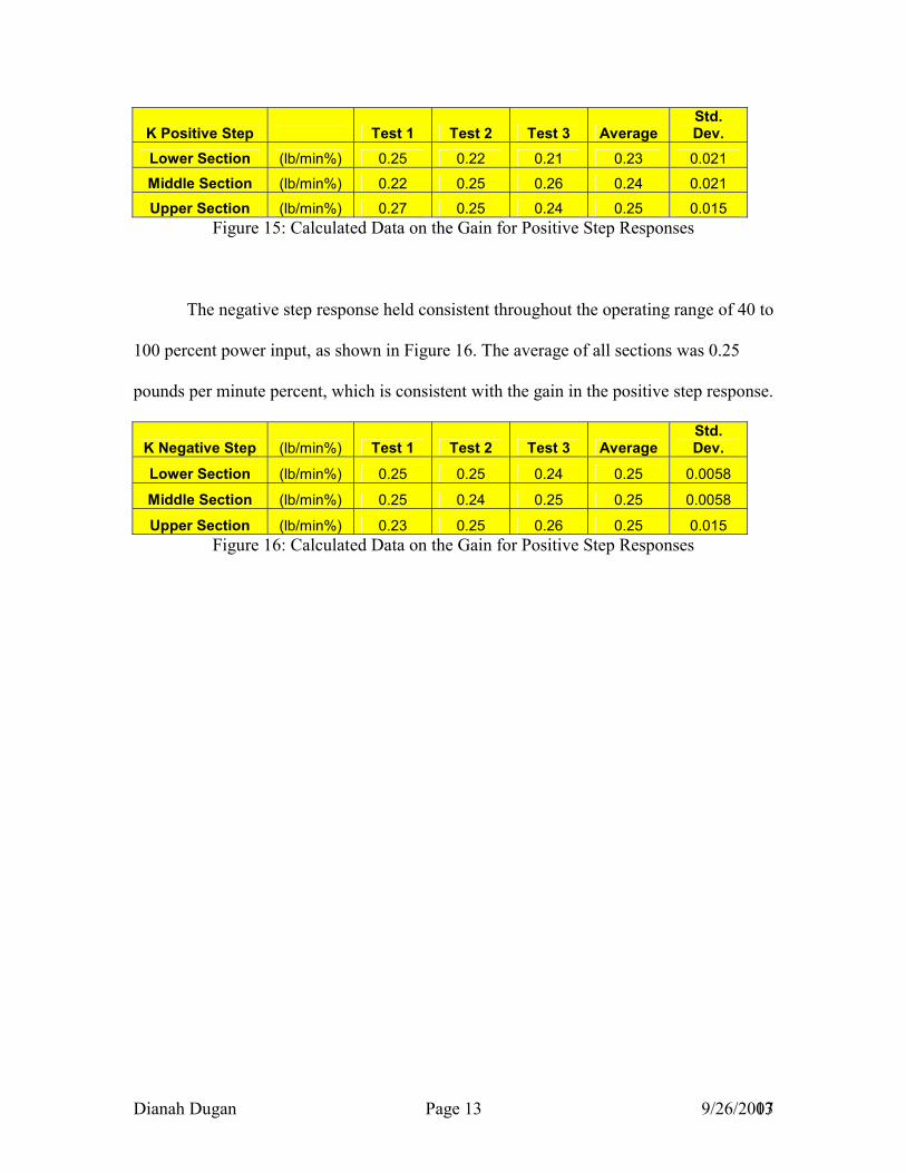
Throughout the operating range of the positive step response, the gain averaged a
value of 0.25 pounds per minute percent, as shown in Figure 15.
Dianah Dugan Page 13 9/26/2007 13
K Positive Step Test 1 Test 2 Test 3 Average Std. Dev.
Lower Section (lb/min%) 0.25 0.22 0.21 0.23 0.021
Middle Section (lb/min%) 0.22 0.25 0.26 0.24 0.021
Upper Section (lb/min%) 0.27 0.25 0.24 0.25 0.015 Figure 15: Calculated Data on the Gain for Positive Step Responses
The negative step response held consistent throughout the operating range of 40 to
100 percent power input, as shown in Figure 16. The average of all sections was 0.25
pounds per minute percent, which is consistent with the gain in the positive step response.
K Negative Step (lb/min%) Test 1 Test 2 Test 3 Average Std. Dev.
Lower Section (lb/min%) 0.25 0.25 0.24 0.25 0.0058
Middle Section (lb/min%) 0.25 0.24 0.25 0.25 0.0058
Upper Section (lb/min%) 0.23 0.25 0.26 0.25 0.015 Figure 16: Calculated Data on the Gain for Positive Step Responses

Dianah Dugan Page 14 9/26/2007 14
Discussion:
The results for the lower section of the operating region, which is between 40 and
60 percent power input, there is a 95 percent confidence that the time constant will be
between 1.03 and 1.37 seconds, the dead time will be between 0.40 and 0.56 seconds, and
the gain will be between 0.21 and 0.25 seconds. The middle section of the operating
region, which is between 60 and 80 percent power input are 95 percent confident of
falling between 1.23 and 1.57 seconds for the time constant, 0.43 and 0.83 seconds for
the dead time, and 0.23 and 0.26 pounds per minute percent for the gain. The results
show that for the upper section of the operating region, which is between 80 and 100
percent power input, there is a 95 percent confidence that the time constant will be
between zero and 1.71 seconds, the dead time will be between 0.23 and 0.57 seconds, and
the gain will be between 0.24 and 0.27 pounds per minute times percent.
For the entire operating range of 40 to 100 percent power, the average gain of the
first order plus dead time parameter agrees with the slope of the steady-state operating
curve of approximately 0.25 pounds per minute percent, both as a positive and negative
step response.
Dianah Dugan Page 15 9/26/2007 15
Conclusions:
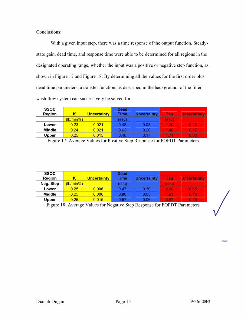
With a given input step, there was a time response of the output function. Steady-
state gain, dead time, and response time were able to be determined for all regions in the
designated operating range, whether the input was a positive or negative step function, as
shown in Figure 17 and Figure 18. By determining all the values for the first order plus
dead time parameters, a transfer function, as described in the background, of the filter
wash flow system can successively be solved for.
SSOC Region K Uncertainty
Dead Time Uncertainty Tau Uncertatinty
(lb/min%) (sec) (sec) Lower 0.23 0.021 0.48 0.08 1.20 0.17 Middle 0.24 0.021 0.63 0.20 1.40 0.17 Upper 0.25 0.015 0.40 0.17 1.71 0.00
Figure 17: Average Values for Positive Step Response for FOPDT Parameters
SSOC Region K Uncertainty
Dead Time Uncertainty Tau Uncertatinty
Neg. Step (lb/min%) (sec) (sec) Lower 0.25 0.006 0.47 0.30 2.00 0.65 Middle 0.25 0.006 0.80 0.05 1.63 0.10 Upper 0.25 0.015 0.57 0.06 0.87 0.15
Figure 18: Average Values for Negative Step Response for FOPDT Parameters

Dianah Dugan Page 16 9/26/2007 16
Appendices:
The following three graphs were obtained and analyzed in the upper region by Dianah
Dugan.
(Step Up #1)
Step Response Graph
75
80
85
90
95
100
10 11 12 13 14 15 16
Time (sec)
Inpu
t (%
)
16
18
20
22
24
Out
put (
lb/m
in)
K = 0.27 t0 = 0.20 τ = 1.71

Dianah Dugan Page 17 9/26/2007 17
(Step Up #2)
Step Response for Experiment #2
75
80
85
90
95
100
10 11 12 13 14 15 16
Time (sec)
Inpu
t (%
)
16
18
20
22
24
Out
put (
lb/m
in)
K = 0.25 t0 = 0.50 τ = 1.71 (Step Up #3)
Step Response for Experiment #3
75
80
85
90
95
100
10 11 12 13 14 15 16
Time (sec)
Inpu
t (%
)
16
18
20
22
24
Out
put (
lb/m
in)
K = 0.24 t0 = 0.50 τ = 1.71

Dianah Dugan Page 18 9/26/2007 18
The following five graphs were obtained and analyzed in the middle region by Ben
Klinger.
(Step Up #4)
Step Response Graph
60
65
70
75
80
85
90
20 22 24 26 28 30 32 34 36 38 40
Time (s)
Pow
er In
put (
%)
10
12
14
16
18
20
22
24
26
28
30
Flow
Out
put (
lb/m
in)
K = 0.22 t0 = 0.75 τ = 1.5
Dianah Dugan Page 19 9/26/2007 19
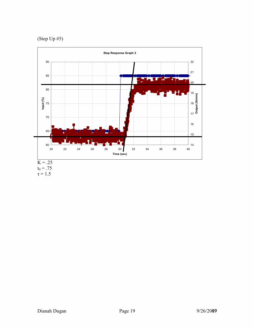
(Step Up #5)
Step Response Graph 2
60
65
70
75
80
85
90
20 22 24 26 28 30 32 34 36 38 40
Time (sec)
Inpu
t (%
)
14
15
16
17
18
19
20
21
22
Out
put (
lb/m
in)
K = .25 t0 = .75 τ = 1.5

Dianah Dugan Page 20 9/26/2007 20
(Step Up #6)
Step Response Graph
60
65
70
75
80
85
90
20 22 24 26 28 30 32 34 36 38 40
Time (sec)
Inpu
t (%
)
10
12
14
16
18
20
22
24
Out
put (
lb/m
in)
K = .26 t0 = .40 τ =1.2

Dianah Dugan Page 21 9/26/2007 21
The following graphs were obtained and analyzed for the lower region by Ben Gordon. (Step Up #7)
Step Response Graph
5051525354555657585960
25 27 29 31 33 35
Time (sec)
Inpu
t (%
)
1010.51111.51212.51313.51414.515
Out
put (
lb/m
in)
K = 0.25 t0 = .39 τ = 1.0 (Step Up #8)
Step Response Graph
5051525354555657585960
25 27 29 31 33 35
Time (sec)
Inpu
t (%
)
1010.51111.51212.51313.51414.515
Out
put (
lb/m
in)
K= 0.22 t0 = 0.54 τ =1.3

Dianah Dugan Page 22 9/26/2007 22
(Step Up #9)
Step Response Graph
5051525354555657585960
25 27 29 31 33 35
Time (sec)
Inpu
t (%
)
1010.51111.51212.51313.51414.515
Out
put (
lb/m
in)
K = 0.21 t0 = .50 τ = 1.3
The following three graphs were obtained and analyzed in the upper region by Dianah
Dugan.

Dianah Dugan Page 23 9/26/2007 23
(Step Down #1)
Step Down #1
80828486889092949698
100
8 10 12 14 16
Time (sec)
Inpu
t (%
)
15
20
25
Out
put (
lb/m
in)
K = 0.23 t0 = 0.60 τ =0.70 (Step Down #2)
Step Down #2
80828486889092949698
100
8 10 12 14 16
Time (sec)
Inpu
t (%
)
15
20
25
Out
put (
lb/m
in)
K = 0.25 t0 = 0.50 τ =1.0

Dianah Dugan Page 24 9/26/2007 24
(Step Down #3)
Step Down #3
75
80
85
90
95
100
8 10 12 14 16
Time (sec)
Inpu
t (%
)
15
20
25
Out
put (
lb/m
in)
K = 0.26 t0 = 0.60 τ =0.90

Dianah Dugan Page 25 9/26/2007 25
The following three graphs were obtained and analyzed in the middle region by Ben
Klinger.
(Step Down #4)
Negative Response 1
60
65
70
75
80
85
90
20 22 24 26 28 30 32 34 36 38 40
Time (s)
Inpu
t (%
)
10
12
14
16
18
20
22
24
Out
put (
lb/m
in)
K = 0.25 t0 = 0.75 τ = 1.5

Dianah Dugan Page 26 9/26/2007 26
(Step Down #5)
Negative Response 2
60
65
70
75
80
85
90
20 22 24 26 28 30 32 34 36 38 40
Time (s)
Inpu
t (%
)
10
12
14
16
18
20
22
24
Out
put (
lb/m
in)
K = 0.24 t0 = 0.85 τ = 1.7 (Step Down # 6)
Negative Response 3
60
65
70
75
80
85
90
20 22 24 26 28 30 32 34 36 38 40
Time (s)
Inpu
t (%
)
10
12
14
16
18
20
22
24
Out
put (
lb/m
in)

Dianah Dugan Page 27 9/26/2007 27
K = 0.25 t0 = 0.80 τ = 1.6 The following graphs were obtained and analyzed for the lower region by Ben Gordon.
(Step Down #7)
Step Down
4042444648505254565860
25 27 29 31 33 35
Time (sec)
Inpu
t (%
)
56789101112131415
Out
put (
lb/m
in)
K = 0.25 t0 = 0.5 τ = 2.0

Dianah Dugan Page 28 9/26/2007 28
(Step Down #8)
Step Down
4042444648505254565860
25 27 29 31 33 35
Time (sec)
Inpu
t (%
)
56789101112131415
Out
put(
lb/m
in)
K= 0.25 t0 = 0.15 τ = 2.6 (Step Down #9)
Step Down
4042444648505254565860
25 27 29 31 33 35
Time (sec)
Inpu
t (%
)
56789101112131415
Out
put (
lb/m
in)
K= 0.24 t0 = 0.75 τ = 1.3

Dianah Dugan Page 29 9/26/2007 29
References:
Figure 1 and Figure 2 were obtained by the following website, as well as information
regarding the background and theory:
http://chem.engr.utc.edu/green-engineering/Filter-Wash/Filter-Wash-System-Detail.htm
Figure 5 and Figure 6 were obtained by the following website:
http://chem.engr.utc.edu/green-engineering/Filter-Wash/Filter-Wash-System-Step.htm
The internet site where the tests were performed:
http://chem.engr.utc.edu/green-engineering/Filter-Wash/Filter-Wash-Step.htm