Steady-state dependability verification for very largesystems

Diana El Rabih Gael Gorgo Nihal Pekergin Jean-Marc Vincent

September 2010

TR–LACL–2010–9

Laboratoire d’Algorithmique, Complexite et Logique (LACL)Departement d’Informatique

Universite Paris 12 – Val de Marne, Faculte des Science et Technologie61, Avenue du General de Gaulle, 94010 Creteil cedex, France

Tel.: (33)(1) 45 17 16 47, Fax: (33)(1) 45 17 66 01

Laboratory of Algorithmics, Complexity and Logic (LACL)University Paris 12 (Paris Est)

Technical Report TR–LACL–2010–9

D. ELRABIH, G. GORGO, N. PEKERGIN, J.M. VINCENTSteady-state dependability verification for very large systems

c© Diana ELRABIH, Gael GORGO, Nihal PEKERGIN, Jean-Marc VINCENT Septem-bre 2010.

Steady-state dependability verification for very large systems ∗

Diana El Rabih1 Gael Gorgo2 Nihal Pekergin1 Jean-Marc Vincent2

1 LACL, University of Paris-Est (Paris 12),61 avenue General de Gaulle 94010, Creteil, France

2 LIG, University of Grenoble (Joseph Fourrier),51, av. Jean Kuntzmann, 38330 MONTBONNOT, France

delrabih@univ-paris12.fr, gael.gorgo@imag.fr,nihal.pekergin@univ-paris12.fr, jean-marc.vincent@imag.fr

Abstract

Probabilistic model checking can be done either by numerical analysis or by simu-lation and statistical methods. In the paper presented in [12], we have compared theefficiency of the numerical model checking implemented in PRISM tool and our statisti-cal model checking approach which combines perfect sampling and statistical hypothesistesting to study the steady-state properties of large Markovian models. In this researchreport we extend this work by considering also the statistical module of the MRMCmodel checker. Therefore the comparisons are established between the numerical modelchecker PRISM, the statistical module of MRMC and our statistical verification engineincluded to the perfect sampler Ψ2. In fact, we compare the efficiency and the scalabilityof these approaches when they are applied to the verification of steady-state propertiesof very large models. We show that our statistical approach using perfect sampling isgenerally more efficient than the two other approaches and it allows us to consider verylarge models and to verify rare event properties efficiently.

Extension of recent work

1. We have enriched the experimental studies. This is done by considering a largerset of input parameters. We have also considered a tandem queue with 10 queuesessentially for the comparison with MRMC statistical model checking module.

2. We have included a section to briefly introduce the new considered tools (MRMCtool) (subsection 4.2) and a section to illustrate the tools differences (subsection4.4).

3. We have included a subsection ( subsection 3.3) for the complexity and the applica-bility of the proposed approach. The section for the brief introduction of tools havebeen extended and MRMC is included. Moreover the paper is reorganised for thesake of readability and sections are extended to make it self-contained (subsection3.3.1).

1 Introduction

Model Checking is a technique for automated verification of software, hardware and networksystems. It has been introduced to verify functional properties of systems expressed in a

∗This work is supported by a french research project CHECKBOUND, ANR-06-SETI-002

3

4

formal logic like Computational Tree Logic (CTL). It is done by accepting as input systemmodels and the properties or specifications that the final system is expected to satisfy and bygiving outputs Yes if the model satisfies given specifications and No otherwise. Probabilisticmodel checking is an extension for the formal verification of systems exhibiting stochastic be-havior. The system model is usually specified as a state transition system, with probabilityvalues attached to transitions, like for example Markov chains. A wide range of quantitativeperformance, reliability, and dependability measures can be specified by means of tempo-ral logics: PCTL for Discrete Time Markov Chains (DTMC) and CSL for Continuous TimeMarkov Chains (CTMC) [3]. Dependability verification of computerised systems is gainingconsiderable importance in daily life. Ensuring minimum breakdown probabilities of, for in-stance, components of real-life computer systems, is vital to fulfil safety requirement specifi-cations. The study of the worst case risk to hit by a safety-critical system at equilibrium inthe system design process is becoming indispensable. In fact, to ensure that a system designmeets its safety requirement specification, one method consists of creating and analysing aformal model of the envisaged design by using model checking techniques. The underlyingstochastic models which are usually Markov chains is defined by high-level formalisms suchas stochastic Petri nets, stochastic process algebras, and queueing networks. We considerqueueing networks as high level formalism for the case studies in this research report.

There are two distinct approaches to perform probabilistic model checking: Numericaltechniques based on computation of transient-state or steady-state distributions of the un-derlying Markov chain [2] and statistical techniques applied on samples obtained by means ofdiscrete event simulation or by measurement. In fact, numerical approach is highly accuratebut it suffers from state space explosion problem while statistical approach can overcome thestate space explosion problem but it provides verification results with probabilistic guaran-tees of correctness. Thus statistical model checking techniques can be seen as an alternativeto numerical techniques and they can be applied when it is infeasible to use numerical tech-niques. In the last years, different statistical model checkers have been proposed [16, 20, 7]especially for properties specified by time-bounded until formulas. Moreover, the statisti-cal model checker MRMC [9] has been proposed and extended to support CSL steady-stateformula. For this formula the probability is estimated based on steady-state simulation ofbottom strongly connected components (BSCCs) and estimates for the probabilities to reachthose BSCCs. On the other hand, the PRISM model checker [8] is largely used. It makesuse of symbolic data representation in order to reduce memory requirements for numericaltechniques and it supports the verification of CSL steady-state formula.

In [6] numerical and statistical techniques have been compared when they are applied tothe verification of time-bounded until formulas in the temporal stochastic logic CSL. In [12],we have compared the efficiency of the numerical model checking implemented in PRISMtool [8] and our statistical model checking approach proposed in [15, 14] which combinesperfect sampling and statistical hypothesis testing to study the steady-state properties oflarge Markovian models. In this research report, we extend this comparison by consideringalso the statistical module of the MRMC model checker. We have also enriched experimentalstudies. This is done by considering a larger set of input parameters. We have also considereda tandem queue with 10 queues essentially for the comparison with MRMC statistical modelchecking module. The significant advantage of perfect sampling is that it permits to analyserare event probabilities efficiently and it provides an unbiased sampling of the steady-statedistribution, hence the accuracy of the verification only depends on the statistical testing. Inother words, we ensure the correctness of our results considering a specified precision level.

This research report is organized as follows: Section 2 briefly presents the perfect sam-

5

pling. In section 3 we present our proposed approach based on perfect sampling. We give abrief introduction of the studied tools in section 4. Section 5 is devoted to the case studies.First we present the models and their validation. Next, we compare and analyze the resultsof our experiments. Finally, in section 6 we summarize the conclusions and provide the futureworks.

2 Perfect Sampling

Let {Xn}n∈N be an irreducible and aperiodic discrete time Markov chain with a finite statespace X and a transition matrix P = (pi,j). Let π denote the steady-state distribution of thechain: π = πP . The evolution of the Markov chain can always be described by a stochasticrecurrence sequence

Xn+1 = η (Xn, en+1) (1)

with {en}n∈N an independent and identically distributed sequence of events en ∈ E , n ∈ N.The transition function η : X × E → X verifies the property that P (η(i, e) = j) = pi,j forevery pair of states (i, j) ∈ X × X and a random event e ∈ E . An execution of the Markovchain is defined by an initial state x0 and a sequence of events {en}n∈N. The sequence ofstates {xn}n∈N defined by equation (1) is called a trajectory.

Algorithm 1 Backward monotone steady-state property-sampling of a Markov chain

Require:η a monotone transition function{en}n≤0 a backward event process{This sequence is previously given or built as the execution of the algorithm}M� the set of extremal elements (Max and Min) of the state space Xrϕ the reward function associated to the checked property ϕ

1: n ← 02: repeat3: {Start from the past at time −2n }4: Z ← M�5: for i = −2n + 1 downto 0 do6: Z ← η(Z, ei) ;7: end for8: { η(2n)(X , e−2n+1→0) ⊂ Z the bounding set of all possible states at time 0 knowing the

event process starting at time −2n }9: n = n+ 1

10: until |rϕ(Z)| = 111: return rϕ(Z) { rϕ(Z) is reduced to one value, 0 or 1 }

Trajectories are generated with the same sequence of events {en}n∈N. If at time t, twotrajectories are in the same state, we say that they couple. Propp and Wilson [11] haveintroduced the perfect/exact sampling method which is based on a backward coupling, alsocalled coupling from the past: by coming from a distant time −τ sufficiently far in the past,if all trajectories (trajectories that come from all possible initial states in X at time −τ) arecoupled in one state at time 0, then the sampled state is exactly distributed according to thestationary distribution. The backward coupling provides steady-state sample in a controlledfinite number of steps, that could not be obtained by a forward coupling scheme unless themodel have a strong stationary time which is rare in our examples [10].

6

The backward coupling called also coupling from the past is especially efficient when theunderlying system is monotone. We first give the definition of monotone systems.

Definition 2.1 Given a partial order � on X , an event e is said to be monotone if it pre-serves the partial ordering � on X . That is

∀(x, y) ∈ X x � y ⇒ η(x, e) � η(y, e)

If all events are monotone, the global system is said to be monotone.

According to an order � on X , there exists a setM� ⊂ X of extremal states (maximaland minimal states). When a Markov chain is monotone, all trajectories issued from X arealways bounded by trajectories issued fromM�. Thus, it is sufficient to compute trajectoriesissued from M� since when they couple, global coupling also occurs. As the size of M� isusually drastically smaller than the size of X , monotone perfect sampling [11] significantlyimproves the sampling time.

Efficiency of simulations is also improved by functional perfect sampling [19]. The algo-rithm sample a reward value, according to a user defined reward function r : X → R; Thealgorithm then stops when all trajectories are in a set of states at time 0 that belong to thesame reward value (going further in the past will inevitably couple in a state that belong tothis reward value). To combine monotone and functional perfect sampling, the reward func-tion r must be monotone, that is x � y ⇒ r(x) � r(y). As |R| is smaller than |X |, thistechnique may lead to an important reduction of the coupling time.

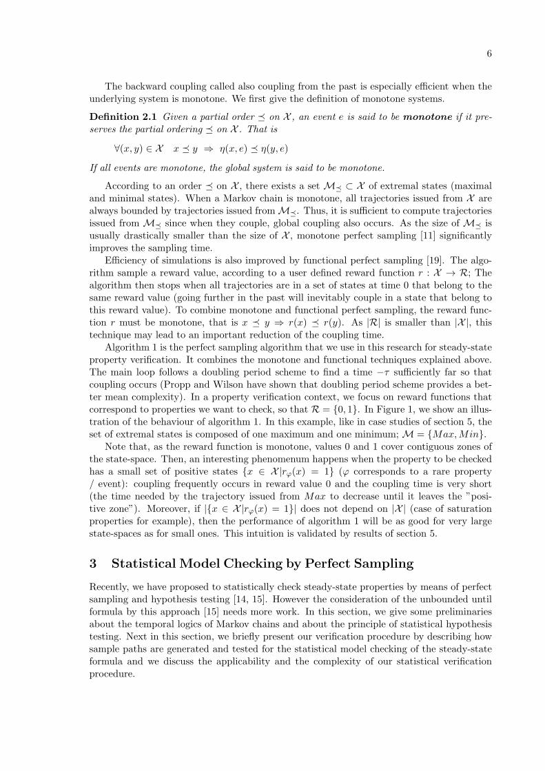
Algorithm 1 is the perfect sampling algorithm that we use in this research for steady-stateproperty verification. It combines the monotone and functional techniques explained above.The main loop follows a doubling period scheme to find a time −τ sufficiently far so thatcoupling occurs (Propp and Wilson have shown that doubling period scheme provides a bet-ter mean complexity). In a property verification context, we focus on reward functions thatcorrespond to properties we want to check, so that R = {0, 1}. In Figure 1, we show an illus-tration of the behaviour of algorithm 1. In this example, like in case studies of section 5, theset of extremal states is composed of one maximum and one minimum;M = {Max,Min}.

Note that, as the reward function is monotone, values 0 and 1 cover contiguous zones ofthe state-space. Then, an interesting phenomenum happens when the property to be checkedhas a small set of positive states {x ∈ X |rϕ(x) = 1} (ϕ corresponds to a rare property/ event): coupling frequently occurs in reward value 0 and the coupling time is very short(the time needed by the trajectory issued from Max to decrease until it leaves the ”posi-tive zone”). Moreover, if |{x ∈ X |rϕ(x) = 1}| does not depend on |X | (case of saturationproperties for example), then the performance of algorithm 1 will be as good for very largestate-spaces as for small ones. This intuition is validated by results of section 5.

3 Statistical Model Checking by Perfect Sampling

Recently, we have proposed to statistically check steady-state properties by means of perfectsampling and hypothesis testing [14, 15]. However the consideration of the unbounded untilformula by this approach [15] needs more work. In this section, we give some preliminariesabout the temporal logics of Markov chains and about the principle of statistical hypothesistesting. Next in this section, we briefly present our verification procedure by describing howsample paths are generated and tested for the statistical model checking of the steady-stateformula and we discuss the applicability and the complexity of our statistical verificationprocedure.

7

Figure 1: Example of a backward monotone steady-state property-sampling

3.1 Temporal logics for Markov chains

In this subsection we give a brief introduction for the considered temporal logics operators.The stochastic behaviour of the underlying system is described by a labelled Markov chain,M, which may be a discret-time Markov chain (DTMC) or a continous-time Markov chain(CTMC). The CSL (resp. PCTL) is a branching-time temporal logic with state and pathformulas over CTMCs (resp. DTMCs) [2]. Thus it is useful to specify performance anddependability measures as logical formulas over Markov chains.

We consider indeed a labelled Markov chainM defined over a finite state space X . LetAP denote the finite set of atomic propositions. L : X → 2AP is the labeling function whichassigns to each state s ∈ X the list of atomic propositions satisfied in this state. Intuitivelyspeaking, when the system is in state s, the properties defined by the set of atomic proposi-tions L(s) assigned to this state are satisfied. The satisfaction operator is denoted by |=. Forall state s ∈ X , s |= true. Atomic proposition a is satisfied by state s (s |= a) iff a ∈ L(s).In this research report, we consider essentially the CSL (resp. PCTL) steady-state opera-tor for long run behaviours of the underlying model. The steady-state operator (formula)S⊲⊳θ(ϕ) (resp. L⊲⊳θ(ϕ)) allows us to analyze the long-run behaviour of the system where θ isa probability threshold, ⊲⊳ a comparison operator: ⊲⊳∈ {<,>,≤,≥}, ϕ is a state formula.

Computing whether s |= S⊲⊳θ(ϕ) amounts to solving a system of linear equations com-bined with graph analysis methods, namely a search for all bottom strongly connected com-ponents (BSCC), which takes O(|X | + |E|) time where |X | denotes the number of states in aCTMC (resp. DTMC) and |E| denotes the number of transitions with non-zero probability.A steady-state analysis is performed for each BSCC, after which the probabilities of reachingthe individual BSCCs are computed. If the sum of steady-state probabilities of states sat-isfying ϕ meets θ, this operator is satisfied. According to [8], steady-state analysis can beperformed with a worst case time complexity of O(|X |3). In this work, we consider ergodicMarkov chainsM, hence there is a unique steady-state distribution independent of the initialstate. Note that for a CSL (resp. PCTL) steady-state formula, the verification for exampleof S≥θ(ϕ) is the same as S≤1−θ(¬ϕ) and also is the same as ¬S<θ(ϕ).

8

3.2 Statistical verification of steady-state properties

For the statistical verification, we have as input parameters: the model defined by a labelledMarkov chain M , the property ϕ (to be verified on each sample). Formally, the CSL (resp.PCTL) steady-state property is specified by ψ = S≥θ(ϕ) Moreover, the threshold θ, the in-difference region δ, the statistical hypothesis testing strength (α, β) are the other input pa-rameters. We propose to apply functional perfect sampling (Algorithm 1, Figure 1), so attime 0, we test if the rewards are coupled at reward 0 or 1. In other words, we test if it is apositive or negative sample. Thus we associate the reward rϕ(x) to each state x ∈ X for thegiven property ϕ:

rϕ(x) = 1, if x |= ϕ (2)

rϕ(x) = 0, otherwise x 6|= ϕ

The statistical decision method that we use is inspired from the Single Sampling Plan(SSP) method [22]. In fact, this decision method counts the number of positive samplesobtained in the considered sample size n, when we test if ϕ is verified (positive sample) ornot (negative sample) on each generated sample path by using functional perfect sampling.Then this decision method provides decision either Yes if the obtained number of positivesamples is greater or equal to the acceptance threshold m (ψ is satisfied) or No otherwise (ψis not satisfied).

3.2.1 Hypothesis Testing

Let p be the probability that the system satisfies the underlying property ϕ, then the verifi-cation problem of ψ = S≥θ(ϕ) can be formulated as an hypothesis testing problem: H : p ≥ θagainst the alternative hypothesis K : p < θ. In fact, the strength of the statistical test wasdetermined by two parameters: α and β, where α is a bound on the probability of accept-ing K when H holds (known as a type I error, or false negative) and β is a bound on theprobability of accepting H when K holds (a type II error, or false positive). In practice, twothresholds, p0 and p1 are defined in terms of the probability threshold, θ, and the half-widthδ of the indifference region: p0 = θ + δ and p1 = θ − δ. Then instead of testing H : p ≥ θagainst K : p < θ, we test H0 : p ≥ p0 against H1 : p ≤ p1. Suppose that we have generated nsamples, and a sample Xi is a positive sample (Xi = 1) if it satisfies ϕ and negative (Xi = 0)otherwise. Xi is a random variable with Bernoulli distribution with parameter p. Thus theprobability to obtain a positive sample is p. In this research report, we only explain the Sin-gle Sampling Plan (SSP) decision method for statistical hypothesis testing, that we apply inthe case studies when using Ψ2.

Single Sampling Plan (SSP): It is based on the acceptance sampling with fixed sam-ple size and with a given acceptance strength (α, β). If

∑ni=1Xi ≥ m, then H0 is accepted

otherwise H1 is accepted, where m is the acceptance threshold. The hypothesis H1 willbe accepted with probability F (m,n, p) and the null hypothesis H0 will be accepted withthe probability 1 − F (m,n, p), where F (m,n, p) is a binomial distribution: F (m,n, p) =∑m

i=1

(

n

i

)

pi(1−p)n−i with

(

n

i

)

is the combination of i from n. It is required that the prob-

ability of accepting H1 when H0 holds is at most α, and the probability of accepting H0 whenH1 holds is at most β. These constraints can be illustrated as below:

• Pr[H1 is accepted | H0 is true] ≤ α which implies F (m,n, p0) ≤ α (C1)

9

• Pr[H0 is accepted | H1 is true] ≤ β which implies 1− F (m,n, p1) ≤ β (C2)

The number of samples n and the acceptance threshold m must be chosen under theseconstraints and can be determined as explained in the following [22]:

The constraints (C1) and (C2) can be expressed as given in [21, 22] where φ−1 is theinverse cumulative distribution function for the standard normal distribution:

• m−np0√(np0(1−p0))

=φ−1(α) (E1)

• - m−np1√(np1(1−p1))

=φ−1(β) (E2)

Then by adding (E1) and (E2), the approximation formula of n to optimise performancecan be derived as follows:

n = (φ−1(α)√(p0(1−p0))+φ−1(β)

√(p1(1−p1)))2

(p0−p1)2(E3)

From [21, 22] the following approximation formula for the inverse normal cumulative dis-tribution function with υ=

√(-log α2) can be used as follows:

φ−1(α) ≈ −υ + a0+a1υ1+b1υ+b2υ2

where a0=2.30753, b1=0.99229, a1=0.27061, b2=0.04481.After computing the sample size n using (E3), the acceptance threshold m can be com-

puted by using either (E1) or (E2).Note that, the acceptance threshold can be approximated to m = ⌊n.θ⌋ where θ is the

threshold of the considered formula.

3.3 Applicability and complexity of proposed approach

Perfect simulation can be applied to monotone systems as proposed in [19, 18] and to nonmonotone systems as proposed in [1]. It can be applied to queuing networks, Markov chains[19, 18] and to stochastic automata networks [4]. Therefore perfect sampling can be appliedto monotone and to non monotone systems modeled by Markov chains, queuing networks orstochastic automata networks. Moreover the functional perfect sampling is particularly usefulin the model checking since we do not look for the exact values but only for the satisfactionor not of a given property.

The complexity of our approach is related to statistical model checking complexity whichdepends on the computed sample size, on the perfect simulation effort (or complexity) and onthe trajectory length in case of path formulas. The computed sample size depends on appliedhypothesis testing decision method. In this work, we use the Single Sampling Plan decisionmethod. Then the sample size will be computed using the approximation formulas given in[22]. It has been shown that if the complexity of the backward simulation algorithm in thenumber of transition function evaluation is bounded by |X |.(2.Eτ∗) [19], then the mean timecomplexity C can be bounded by C ≤ |X |.(2.Eτ∗).cη where τ∗ is the coupling time of thebackward scheme (coupling from the past scheme), |X | is the state space size, cη is the meancomputation cost of η(x, e). The memory complexity (storage of the set of generated events)is bounded by 2Eτ∗ and could be reduced to Elog2τ

∗ + 1 [19].Thus the complexity of the perfect simulation is clearly modest in case of monotone sys-

tems because we consider only maximal and minimal states as initial values among all states.

10

In fact, the simulation time reduction is proportional to the size of the state space in thiscase [18], which is usually very large. It has been shown in [18] when studying coupling timedistribution, that simulation times per sample for the studied queueing networks examplesare just a few milli-seconds on a standard PC. In case of non monotone systems, it has beenshown in [1] that there is only a need to compute two trajectories: an infimum and supre-mum envelopes, then the complexity of perfect simulation in this case will be also modest.Moreover, because of the independence of generated samples, the perfect simulation methodcan be parallelized efficiently [4].

4 Probabilistic Model Checking Tools

We now give a brief presentation of the considered tools.

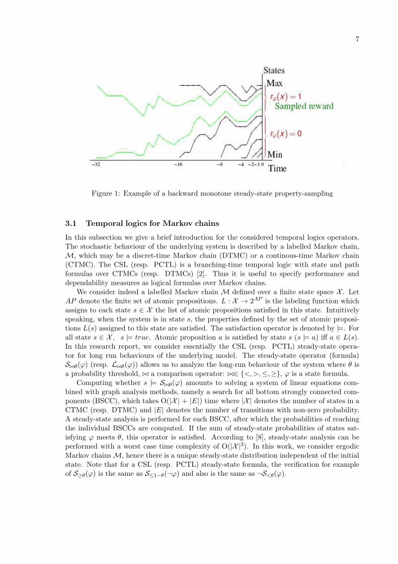
4.1 PRISM: Probabilistic Symbolic Model Checker

PRISM [8] is a largely used probabilistic model checker developped at the University of Ox-ford (http://www.prismmodelchecker.org/). It supports three types of probabilistic mod-els: discrete-time Markov chains (DTMCs), continuous-time Markov chains (CTMCs) andMarkov decision processes (MDPs). PRISM has been used to analyse systems from a widerange of application domains, including communication and multimedia protocols, randomiseddistributed algorithms, security protocols, biological systems and many others. Models aredescribed using the PRISM language, a high level language. PRISM supports automatedanalysis of a wide range of quantitative properties of these models. In fact, the propertyspecification language incorporates the temporal logics PCTL, CSL.

PRISM is a based on numerical techniques solving a system of linear equations combinedwith graph analysis methods, namely a search for all bottom strongly connected components(BSCC). It also features discrete-event simulation functionality for generating approximateresults to quantitative analysis but it does not support steady-state properties.

In addition, PRISM incorporates symbolic data structures and algorithms used for statespace representation, based on BDDs (Binary Decision Diagrams) and MTBDDs (Multi-Terminal Binary Decision Diagrams). For numerical computation, PRISM includes threeseparate engines making varying use of symbolic methods. These engines use different datastructures: The first engine generates an MTBDD to represent the transition matrix, thesparse engine permits to convert the transition matrix to a sparse matrix. The hybrid en-gine is generally faster than MTBDD one, and while handling larger systems is expected tobe faster and to consume less memory than sparse matrices, and hence is the one used inthis research report. The user interface and parsers of PRISM are written in Java; the corealgorithms are mostly implemented in C++.

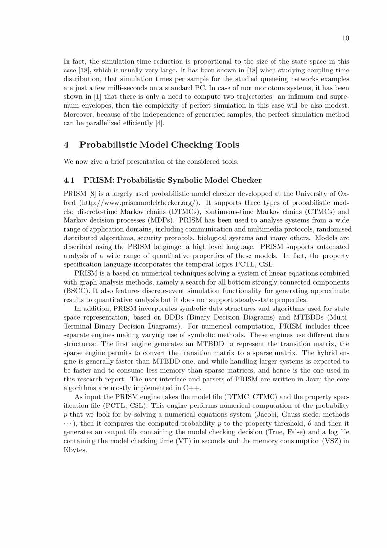
As input the PRISM engine takes the model file (DTMC, CTMC) and the property spec-ification file (PCTL, CSL). This engine performs numerical computation of the probabilityp that we look for by solving a numerical equations system (Jacobi, Gauss siedel methods· · · ), then it compares the computed probability p to the property threshold, θ and then itgenerates an output file containing the model checking decision (True, False) and a log filecontaining the model checking time (VT) in seconds and the memory consumption (VSZ) inKbytes.

11

Figure 2: The PRISM Tool

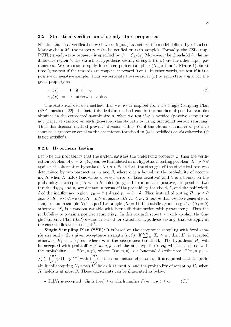
4.2 MRMC: Markov Reward Model Checker

MRMC [9] stands for Markov Reward Model Checker developped at the University of Twente(http://www.mrmc-tool.org/trac/). It has first implemented numerical model-checking tech-niques for DTMC and CTMC models. It is a command-line tool implemented in C. MRMCrepresents the state space by sparse matrices. In fact, it uses simple but high-performancedata structures, such as: a slightly modified version of the well-known compressed-row, compressed-column representation of probability (rate) matrices, and bit vectors for representing sets ofstates. Since v1.4.1, it has a full support for the statistical model checking of CSL propertieson CTMC models.

For the steady-state formulae the probability is estimated based on steady-state sim-ulation (based on the regeneration method) [9] of bottom strongly connected components(BSCCs) and estimates for the probabilities to reach those BSCCs. In fact, the formula isverified by estimating its probability using a confidence interval of desired width and thenby comparing it against the formula probability bound. MRMC does not employ standardsequential confidence interval but rather emulates it by gradually increasing the sample size.

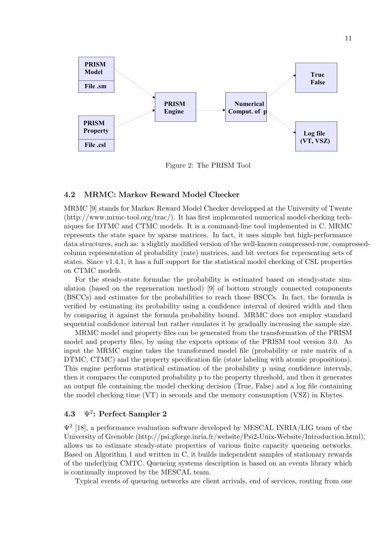
MRMC model and property files can be generated from the transformation of the PRISMmodel and property files, by using the exports options of the PRISM tool version 3.0. Asinput the MRMC engine takes the transformed model file (probability or rate matrix of aDTMC, CTMC) and the property specification file (state labeling with atomic propositions).This engine performs statistical estimation of the probability p using confidence intervals,then it compares the computed probability p to the property threshold, and then it generatesan output file containing the model checking decision (True, False) and a log file containingthe model checking time (VT) in seconds and the memory consumption (VSZ) in Kbytes.

4.3 Ψ2: Perfect Sampler 2

Ψ2 [18], a performance evaluation software developed by MESCAL INRIA/LIG team of theUniversity of Grenoble (http://psi.gforge.inria.fr/website/Psi2-Unix-Website/Introduction.html),allows us to estimate steady-state properties of various finite capacity queueing networks.Based on Algorithm 1 and written in C, it builds independent samples of stationary rewardsof the underlying CMTC. Queueing systems description is based on an events library whichis continually improved by the MESCAL team.

Typical events of queueing networks are client arrivals, end of services, routing from one

12

Figure 3: The MRMC Tool

13

queue to another, negative clients, and batch means arrivals. Complex routing strategies hadbeen captured in a common framework, based on index functions [17], so that a large scope ofmonotone queueing networks can be studied. Moreover, the sandwiching principle of mono-tone backward coupling had been generalized to non-monotone queueing networks (envelopestechniques [1]) and implemented in Ψ2. This tool has been used in various domains, includ-ing networks dimensioning, telecommunications systems, resource brokering problems, etc.Ψ2 is well suited for probabilistic model checking, and in particular for steady state formulaverification, since it provides an unbiased sampling of stationary rewards and guarantees in-dependence of samples. It is specifically suited for rare event probability estimation, as wasalready done in [17].

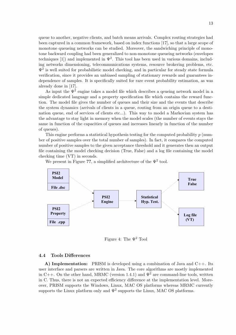
As input the Ψ2 engine takes a model file which describes a qeueing network model in asimple dedicated language and a property specification file which contains the reward func-tion. The model file gives the number of queues and their size and the events that describethe system dynamics (arrivals of clients in a queue, routing from an origin queue to a desti-nation queue, end of services of clients etc...). This way to model a Markovian system hasthe advantage to stay light in memory when the model scales (the number of events stays thesame in function of the capacities of queues and increases linearly in function of the numberof queues).

This engine performs a statistical hypothesis testing for the computed probability p (num-ber of positive samples over the total number of samples). In fact, it compares the computednumber of positive samples to the given acceptance threshold and it generates then an outputfile containing the model checking decision (True, False) and a log file containing the modelchecking time (VT) in seconds.

We present in Figure ??, a simplified architecture of the Ψ2 tool.

Figure 4: The Ψ2 Tool

4.4 Tools Differences

A) Implementation: PRISM is developed using a combination of Java and C++. Itsuser interface and parsers are written in Java. The core algorithms are mostly implementedin C++. On the other hand, MRMC (version 1.4.1) and Ψ2 are command-line tools, writtenin C. Thus, there is not an expected efficiency difference at the implementation level. More-over, PRISM supports the Windows, Linux, MAC OS platforms whereas MRMC currentlysupports the Linux platform only and Ψ2 supports the Linux, MAC OS platforms.

14

B) Model and specification: For PRISM, system models are described using the PRISMprogramming language, which is a high-level state-based description language. In this lan-guage a system is described as the parallel composition of a set of modules. A module stateis determined by a set of finite-range variables and its behaviour is given using a guarded-command based notation. Communication between modules takes place either via globalvariables or synchronisation over common action labels. PRISM is able to export models inmany different formats, including the ones accepted by MRMC. The PRISM model descrip-tion is translated (by the tool) into one of the three supported probabilistic models (DTMC,CTMC, MDP). In PRISM, properties can be specified using PCTL (for DMTCs and MDPs)or CSL (for CTMCs). It is possible to either determine if a probability satisfies a given boundor obtain the actual value. There is also support for the specification and analysis of prop-erties based on costs and rewards. For MRMC, input models are described in a text formatwhere each line specifies one transition consisting of an action name, the source state, thetarget state, the transition rate and the type, which is set to M (Markovian). Input model isdefined by a .tra file and the state labelling by a .lab file. MRMC supports DTMC, CTMCas input models, and their reward extensions DMRM, CMRM. In MRMC, properties can bespecified using PCTL, CSL temporal logics and their reward extensions PRCTL, CSRL. ForΨ2, input models are described in a text format (.dsc file) where lines specifies number ofqueues, events type and number, transition consisting of an event execution. In Ψ2, DTMCand CTMC are supported as input models and properties can be specified by PCTL andCSL temporal logics. Ψ2 can only verify properties in the initial state of the model. Thus,the results correspond to model checking formulae in the initial state. Moreover, it does notprovide the probability estimates.

C) Verification algorithms: PRISM is based on symbolic and numerical algorithms rep-resenting the state space implicitly using a compact data structure and offering a range ofmethods for solving a system of linear equations. The advantage of using numerical meth-ods is their high accuracy, but the drawback is that they require a large amount of memory(caused by the state-space explosion problem). MRMC and Ψ2 are based on statistical algo-rithms using simulation and sampling. They will then estimate if the property holds basedon the generated samples. Choosing a better confidence level (lower probability of gettingwrong answers) results in more samples being taken, which in turn causes the model checktime of the statistical method to increase. Then this method will obviously not provide thehigh level of accuracy as in numerical methods, since it is statistical in nature.

D) State space representation: PRISM (Hybrid engine) use a combination of Multi Ter-minal Binary Decision Diagram (MTBDD) and sparse matrix for state space representation.MRMC represents the state space by sparse matrices by using simple but high-performancedata structures, such as: a slightly modified version of the well-known compressed-row, compressed-column representation of probability (rate) matrices, and bit vectors for representing sets ofstates. In Ψ2, instead of building a complete state-space and verifying properties in eachstate, the statistical method implemented in Ψ2 uses the model description to generate sam-ple execution paths. In fact, Ψ2 unlike PRISM and MRMC has on-the-fly model generation.PRISM and MRMC accept pre-generated CTMCs, and thus their memory values should de-pend on the model size.

15

E) Statistical techniques: The statistical algorithm of MRMC implements criteria dif-ferent from the acceptance criteria used in model checking by hypothesis testing used in Ψ2.The difference between these two statistical techniques, is the requirement to use confidenceinterval of the width ≺ δ, whereas under the same conditions in hypothesis testing we wouldhave to use the indifference region of the width less than only 2.δ. This can cause MRMCmodel checking algorithms to require more samples than needed for the ones based on hy-pothesis testing used in Ψ2.

G) Simulation methods: The simulation by regeneration method used in MRMC hassome disadvantages over the perfect simulation used in Ψ2. First, the lengths of the regener-ation cycle are unpredictable. Then it is not possible to plan the simulation time beforehand.Second, finding the regeneration point is not trivial since it may require a lot of checking afterevery event. In fact, when the number of queues in a regenerative system increases, the regen-eration points become rarer and regeneration cycles become longer. However, not all systemsare regenerative. Third, many of variance reduction techniques such as antithetic variablesfor example cannot be used due to the variable length of the regeneration cycles. Fourth,in the regeneration method, the mean and variance estimators are biased in the sense thattheir expected values from a random sampling are not equal to the quantity being estimated.Finaly, when using the regeneration method for analysing rare events (rare probabilities), thesimulation become longer.

5 Experimental Comparison Study

We now evaluate four case studies, taken from Ψ2 and PRISM benchmarks, on which we willbase our performance and scalability comparison. In fact, we verify the steady-state formulafor these four case studies using the numerical approach implemented in PRISM tool, thestatistical approach implemented in MRMC tool, and our statistical approach implementedin Ψ2 tool, by varying the problem size (state space size related to the maximal queue capac-ity), the precision parameters of the considered verification tools, and the number of queues(number of events). We illustrate the verification time in seconds for these case studies asa function of the maximal queue capacity (state space size) and we determine the memorylimit for each case when using the verification tools. Since the considered Markovian modelsare ergodic (by construction), thus the steady-state probabilities are independent of the ini-tial state. Thus, the considered steady-state formula is satisfied or not whatever the initialstates. In fact, these four case studies are modelised by three formal models as described inthe following.

5.1 Tandem network

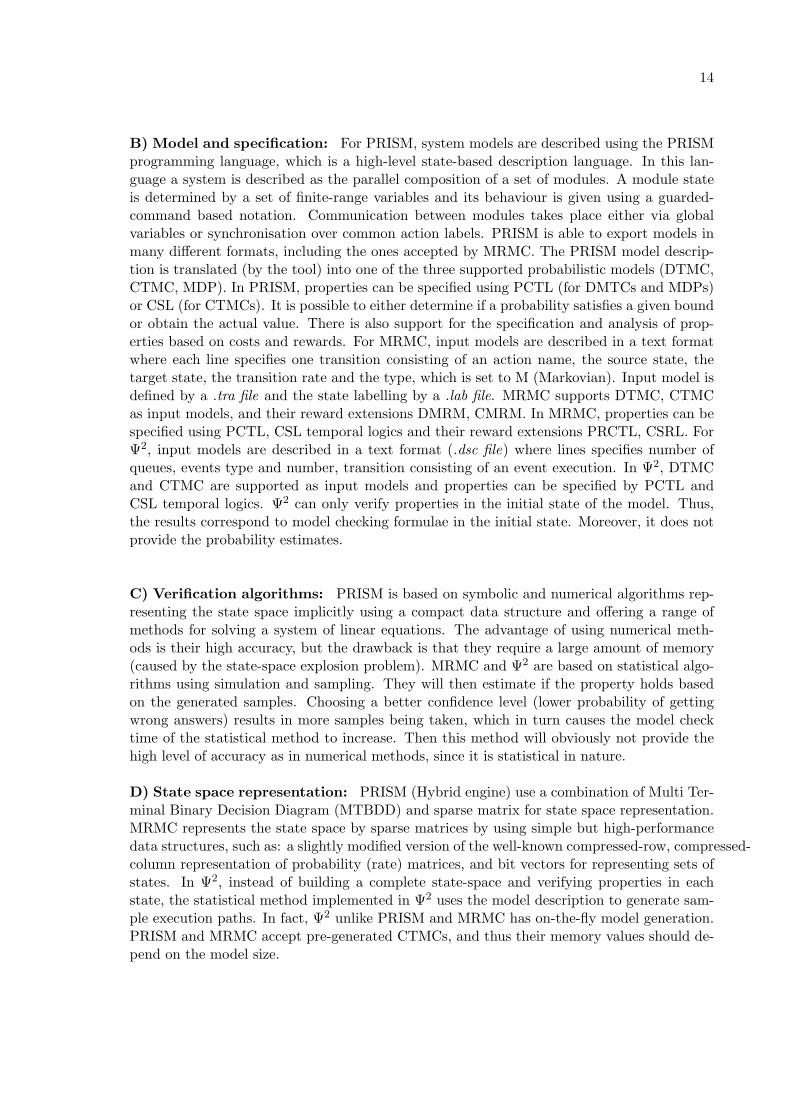
This model is taken from the Ψ2 benchmark. We have implemented and validated [12, 13]this model as a PRISM model. We consider b finite buffers in tandem where each buffer is aM/M/1/Nmax queue (Figure 5). This tandem network is defined by an input Poisson process(rate λ) at the first stage and by an exponential service rates in each stage. Let µi be theservice rate in stage i. In fact, the end of service in stage i, 1 ≤ i ≤ b−1 constitutes an arrivalto stage i + 1. The packet acceptance mechanism is the rejection: a packet which arrives toa full buffer is lost. Denote by Nmax the maximal capacity of each queue. The state spaceassociated with this tandem network is defined by (Nmax + 1)b. Three types of events occur

16

in this system : Arrival from exterior, end of service in stage i and arrival to stage i+1, anddeparture to exterior after end of service in the last stage. The monotonicity of these eventsis shown in [17]. Thus this considered model is monotone. Let Ni, 1 ≤ i ≤ b be the number of

Figure 5: Tandem network

packets in buffer i. Thus (N1, N2, · · · , Nb) is a CTMC of size (Nmax +1)b . In the sequel, wedenote by s = (n1, n2, · · · , nb) a state of this Markov chain. We are interested in saturationproperties in the last stage and we can also conclude about availability properties. Since allearlier stages must be taken into account to compute saturation probabilities in the last bufferb, we must consider whole Markov chain of (Nmax + 1)b size. Thus the numerical complexityto solve the underlying model increases rapidly with Nmax. We define the following atomicproposition related to buffer b : last-full is valid if the bth buffer is full. Based on this atomicproposition, we check the following steady-state formula: S≤θ (last-full) to check whether theprobability that buffer b is full in steady-state is less than θ or not.

5.2 Multistage Delta Network (MDN)

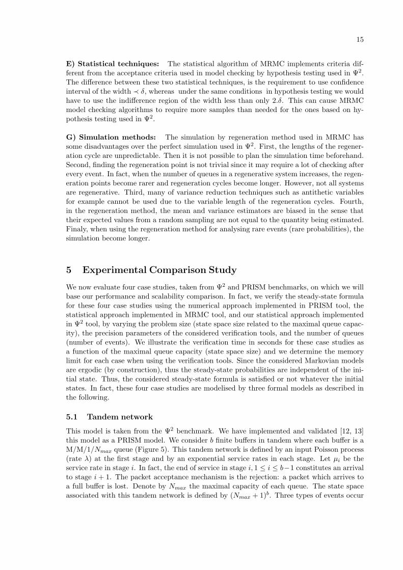
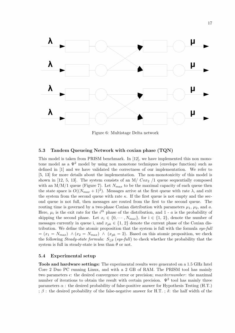
This model is taken from the Ψ2 benchamrk. We have implemented and validated [12, 13]this model as a PRISM model. The considered model is a delta network with y stages andz buffers at each stage (Figure 6). Thus the total number of queues (buffers) is b = y ∗ z.With Markovian arrival and service hypothesis, the model can be defined as a CTMC witha state vector (N1, N2, · · · , Nb) where Ni is the number of packets in the ith queue. Thesize of the state space is (Nmax + 1)b, if the maximum queue size is Nmax. We suppose anhomogeneous input trafic with arrival rate λ to the first stage and service rate is µ in eachqueue. The routing policy is rejection (packets are lost if the queue is full) and at the end ofa service in stage i the routing service rates to stage i + 1 are (τrout1, τrout2) with 1 ≤ i ≤y − 1. There are events (z external arrivals at the 1st stage, z departures at the yth stage, 2× z routing events between stage i and stage i + 1 with 1 ≤ i ≤ y − 1. The monotonicityof these events and thus the monotonicity of this model has been shown in [17]. State labelsare defined through atomic propositions depending on the number of packets in queues. Fora given k ∈ {0, · · · , Nmax}, the atomic proposition ai(k) is true if Ni ≥ k and false otherwise.For example, ai (Nmax) is true if the ith buffer is full. The underlying CTMC is labelledwith these atomic propositions depending on the considered property. It is indeed possibleto express different interesting availability and reliability measures for the underlying systemby means of these atomic propositions. For instance, with formula ψ=S<θ(ai (Nmax)) wecan check the saturation property in the ith buffer to see whether the long run saturationprobability of the ith buffer is less than θ or not. This allows us also to check the availabilityproperty, S>1−θ(¬ ai(Nmax)). We define the atomic proposition last-stage-full that is validif at least a queue at the second level is saturated. Thus it is defined as the disjunction ofatomic propositions ai(Nmax), 4 ≤ i ≤ 7. Based on this atomic proposition, we considerto verify the following steady-state formula ψ = S<θ(last-stage-full) that let us to studysaturation or availability properties (S>1−θ(¬ last-stage-full)).

17

Figure 6: Multistage Delta network

5.3 Tandem Queueing Network with coxian phase (TQN)

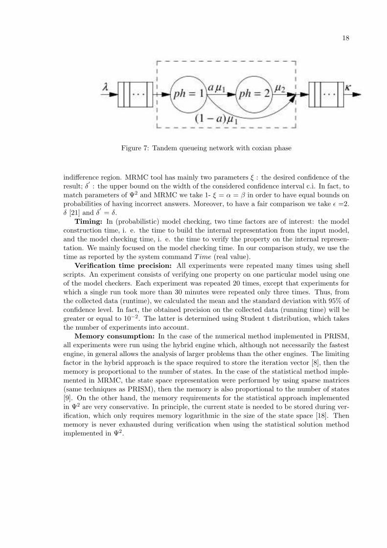
This model is taken from PRISM benchmark. In [12], we have implemented this non mono-tone model as a Ψ2 model by using non monotone techniques (envelope function) such asdefined in [1] and we have validated the correctness of our implementation. We refer to[5, 13] for more details about the implementation. The non-monotonicity of this model isshown in [12, 5, 13]. The system consists of an M/ Cox2 /1 queue sequentially composedwith an M/M/1 queue (Figure 7). Let Nmax to be the maximal capacity of each queue thenthe state space is O((Nmax + 1)2). Messages arrive at the first queue with rate λ, and exitthe system from the second queue with rate κ. If the first queue is not empty and the sec-ond queue is not full, then messages are routed from the first to the second queue. Therouting time is governed by a two-phase Coxian distribution with parameters µ1, µ2, and a.Here, µi is the exit rate for the ith phase of the distribution, and 1 - a is the probability ofskipping the second phase. Let xi ∈ {0, · · · , Nmax}, for i ∈ {1, 2}, denote the number ofmessages currently in queue i, and xph ∈ {1, 2} denote the current phase of the Coxian dis-tribution. We define the atomic proposition that the system is full with the formula sys-full= (x1 = Nmax) ∧ (x2 = Nmax) ∧ (xph = 2). Based on this atomic proposition, we checkthe following Steady-state formula: S≤θ (sys-full) to check whether the probability that thesystem is full in steady-state is less than θ or not.

5.4 Experimental setup

Tools and hardware settings: The experimental results were generated on a 1.5 GHz IntelCore 2 Duo PC running Linux, and with a 2 GB of RAM. The PRISM tool has mainlytwo parameters ǫ: the desired convergence error or precision; maxiternumber: the maximalnumber of iterations to obtain the result with certain precision. Ψ2 tool has mainly threeparameters α : the desired probability of false-positive answer for Hypothesis Testing (H.T.); β : the desired probability of the false-negative answer for H.T. ; δ: the half width of the

18

Figure 7: Tandem queueing network with coxian phase

indifference region. MRMC tool has mainly two parameters ξ : the desired confidence of theresult; δ

′

: the upper bound on the width of the considered confidence interval c.i. In fact, tomatch parameters of Ψ2 and MRMC we take 1- ξ = α = β in order to have equal bounds onprobabilities of having incorrect answers. Moreover, to have a fair comparison we take ǫ =2.δ [21] and δ

′

= δ.Timing: In (probabilistic) model checking, two time factors are of interest: the model

construction time, i. e. the time to build the internal representation from the input model,and the model checking time, i. e. the time to verify the property on the internal represen-tation. We mainly focused on the model checking time. In our comparison study, we use thetime as reported by the system command Time (real value).

Verification time precision: All experiments were repeated many times using shellscripts. An experiment consists of verifying one property on one particular model using oneof the model checkers. Each experiment was repeated 20 times, except that experiments forwhich a single run took more than 30 minutes were repeated only three times. Thus, fromthe collected data (runtime), we calculated the mean and the standard deviation with 95% ofconfidence level. In fact, the obtained precision on the collected data (running time) will begreater or equal to 10−2. The latter is determined using Student t distribution, which takesthe number of experiments into account.

Memory consumption: In the case of the numerical method implemented in PRISM,all experiments were run using the hybrid engine which, although not necessarily the fastestengine, in general allows the analysis of larger problems than the other engines. The limitingfactor in the hybrid approach is the space required to store the iteration vector [8], then thememory is proportional to the number of states. In the case of the statistical method imple-mented in MRMC, the state space representation were performed by using sparse matrices(same techniques as PRISM), then the memory is also proportional to the number of states[9]. On the other hand, the memory requirements for the statistical approach implementedin Ψ2 are very conservative. In principle, the current state is needed to be stored during ver-ification, which only requires memory logarithmic in the size of the state space [18]. Thenmemory is never exhausted during verification when using the statistical solution methodimplemented in Ψ2.

19

5.5 Experimental results

5.5.1 Tandem network verification results

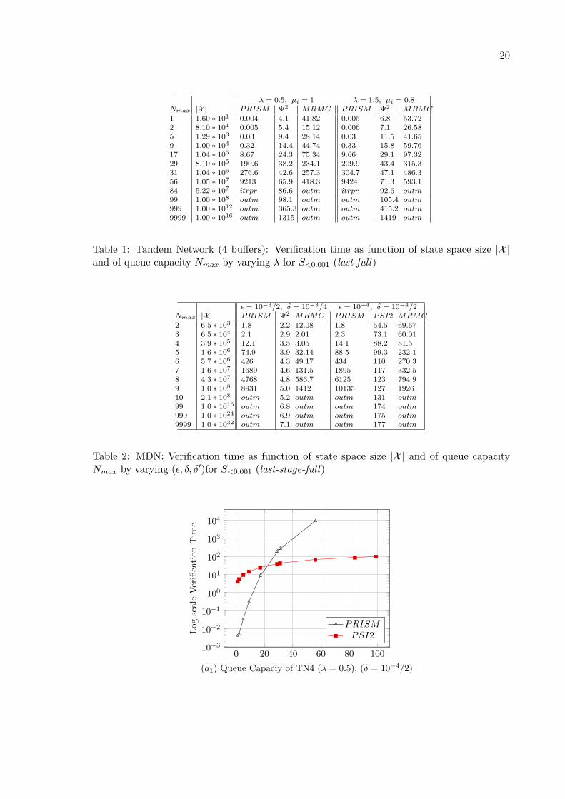
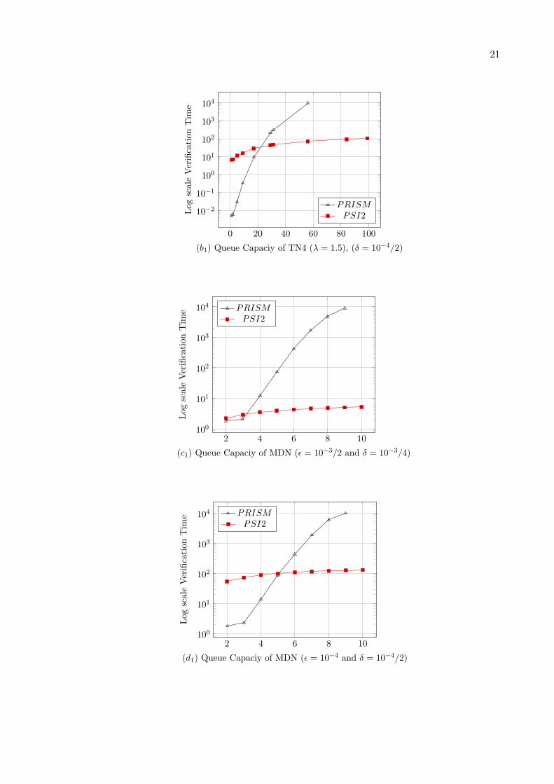
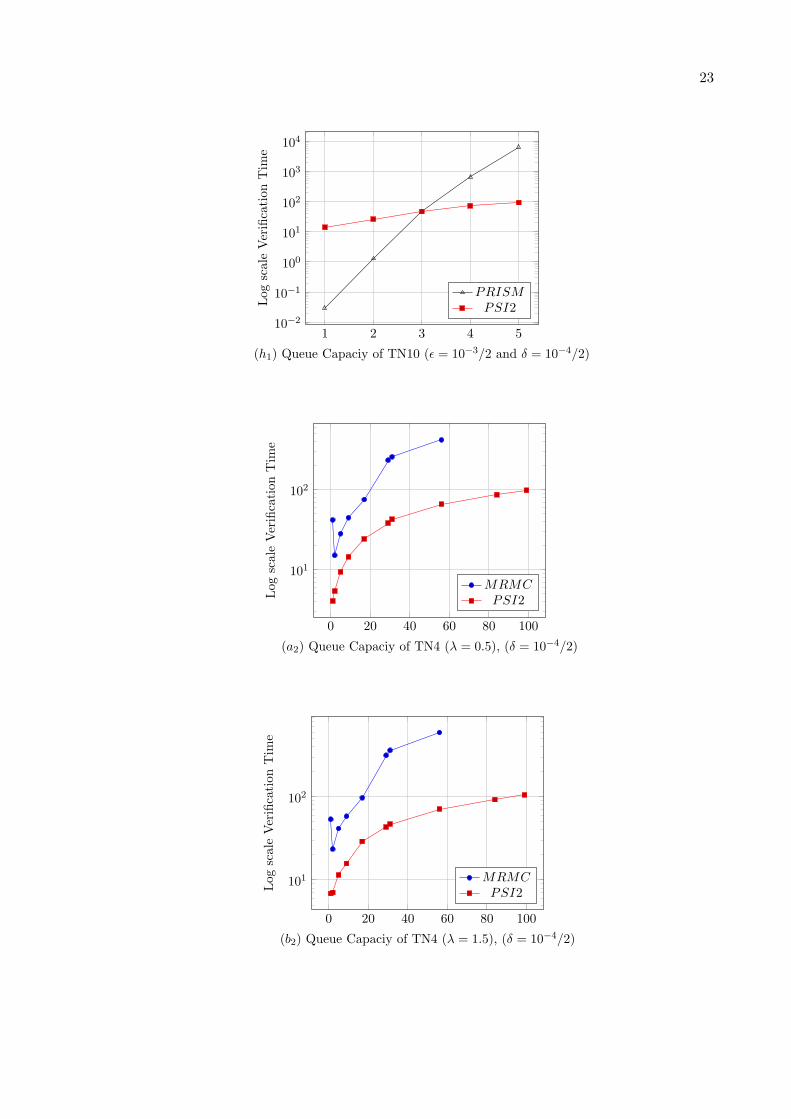
For numerical application, first we consider b = 4 and λ = {0.5 or 1.5}, all service rates willbe state-independent with rate µi = 1, 1 ≤ i ≤ b. We give in Table 1 for b = 4, θ = 0.001and ǫ = {10−3/2 or 10−4}, the numerical verification time for the considered steady-stateformula S<θ (last-full) by using PRISM Hybrid engine and Jacobi iterative method. Also wegive in the same table for b = 4, θ = 0.001, δ = δ′ = {10−3/4 or 10−4/2} respectively, and1− ξ = α = β = 10−2 the verification time for the same steady-state formula S<θ (last-full)by using statistical verification methods implemented in MRMC and in Ψ2 (section 3). Nextwe present part of these results (Nmax ≤ 99) in the Figures (a1), (a2), (b1) and (b2). In fact,for Nmax = 99 we obtain an out of memory message with PRISM and with MRMC.

Moreover, we consider b = 10 and for the same values of model parameters and of toolsparameters as in the case of b = 4, we give in Table 4 the numerical verification time byusing PRISM Hybrid engine and Jacobi iterative method. Also we give in the same table forb = 10, the verification time for the steady-state formula S<θ (last-full) by using statisticalverification methods implemented in MRMC and in Ψ2 (section 3). Next we present part ofthese results (Nmax ≤ 6) in the Figures (g1), (g2), (h1) and (h2). In fact, for b = 10 we obtainan out of memory message with PRISM and with MRMC for Nmax = 6.

In all of the tables and figures we denote by:PRISM : numerical model checking time in seconds for the steady-state formula by using

PRISM hybrid engine.Ψ2 : statistical model checking time in seconds for the steady-state formula by using our

verification method (section 3) implemented in Ψ2 engine.MRMC : statistical model checking time in seconds for the steady-state formula by using

MRMC engine. Note that we have used MRMC with PHC options, where P (pure simula-tion), H (hybrid regenaration method), C (fixed sample size) options.

outm : an out of memory message in PRISM tool or in MRMC tool.itrpr: a maximal iteration number problem (we consider maxiternumber = 100000 in

PRISM tool).

5.5.2 Multistage delta network (MDN) verification results

For numerical application, we consider y = 2 stages and z = 4 buffers/stage, λ = 0.9,µ = 1, (τrout1, τrout2) = (0.8, 0.6). Note that, for y = 4 stages and z = 8 buffers/stage wehave obtain efficient results by using Ψ2 [15, 14] while it is not possible to do numerical modelchecking PRISM nor statistical model checking MRMC (memory problem for Nmax=1) inthis case due to the huge state space size O((Nmax + 1)32).

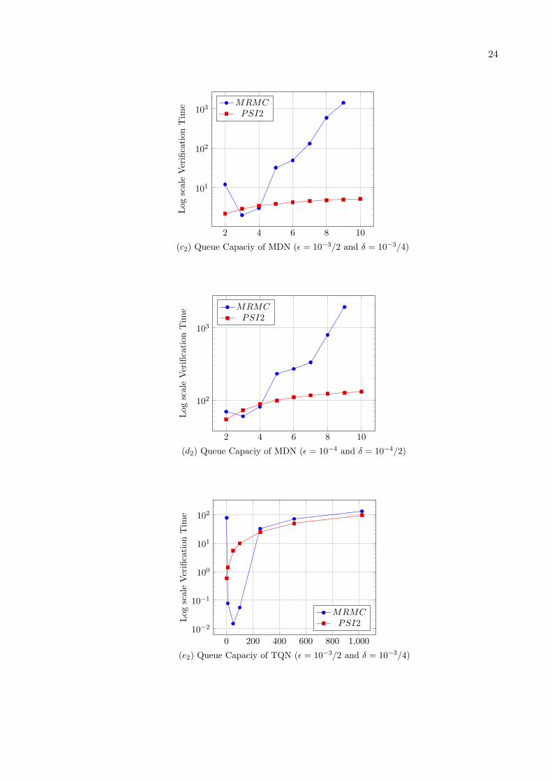
We give in Table 2 for θ = 0.001 and for ǫ = {10−3/2 or 10−4}, the numerical verificationtime for the considered steady-state formula S<θ (last-stage-full) by using PRISM Hybridengine and Jacobi iterative method. Also we give in the same table for θ = 0.001, δ =δ′ = {10−3/4 or 10−4/2} respectively, and 1 − ξ = α = β = 10−2, the verification time forthe same steady-state formula S<θ (last-stage-full) by using statistical verification methodsimplemented in MRMC and in Ψ2 (section 3). We present part of these results (Nmax ≤ 10)in the Figures (c1), (c2), (d1) and (d2). In fact, for Nmax = 10 we obtain an out of memorymessage with PRISM and with MRMC.

20

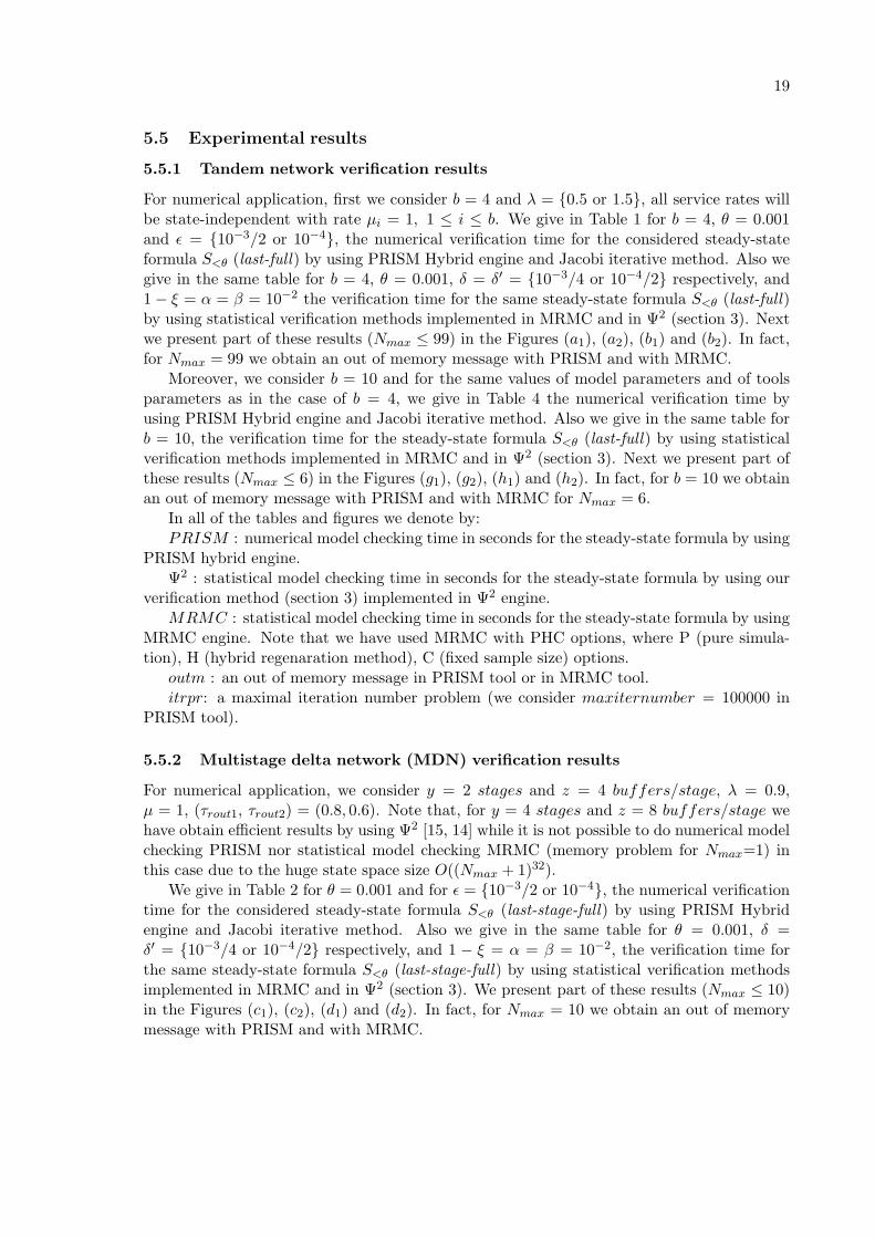
λ = 0.5, µi = 1 λ = 1.5, µi = 0.8Nmax |X | PRISM Ψ2 MRMC PRISM Ψ2 MRMC1 1.60 ∗ 101 0.004 4.1 41.82 0.005 6.8 53.722 8.10 ∗ 101 0.005 5.4 15.12 0.006 7.1 26.585 1.29 ∗ 103 0.03 9.4 28.14 0.03 11.5 41.659 1.00 ∗ 104 0.32 14.4 44.74 0.33 15.8 59.7617 1.04 ∗ 105 8.67 24.3 75.34 9.66 29.1 97.3229 8.10 ∗ 105 190.6 38.2 234.1 209.9 43.4 315.331 1.04 ∗ 106 276.6 42.6 257.3 304.7 47.1 486.356 1.05 ∗ 107 9213 65.9 418.3 9424 71.3 593.184 5.22 ∗ 107 itrpr 86.6 outm itrpr 92.6 outm99 1.00 ∗ 108 outm 98.1 outm outm 105.4 outm999 1.00 ∗ 1012 outm 365.3 outm outm 415.2 outm9999 1.00 ∗ 1016 outm 1315 outm outm 1419 outm

Table 1: Tandem Network (4 buffers): Verification time as function of state space size |X |and of queue capacity Nmax by varying λ for S<0.001 (last-full)

ǫ = 10−3/2, δ = 10−3/4 ǫ = 10−4, δ = 10−4/2Nmax |X | PRISM Ψ2 MRMC PRISM PSI2 MRMC2 6.5 ∗ 103 1.8 2.2 12.08 1.8 54.5 69.673 6.5 ∗ 104 2.1 2.9 2.01 2.3 73.1 60.014 3.9 ∗ 105 12.1 3.5 3.05 14.1 88.2 81.55 1.6 ∗ 106 74.9 3.9 32.14 88.5 99.3 232.16 5.7 ∗ 106 426 4.3 49.17 434 110 270.37 1.6 ∗ 107 1689 4.6 131.5 1895 117 332.58 4.3 ∗ 107 4768 4.8 586.7 6125 123 794.99 1.0 ∗ 108 8931 5.0 1412 10135 127 192610 2.1 ∗ 108 outm 5.2 outm outm 131 outm99 1.0 ∗ 1016 outm 6.8 outm outm 174 outm999 1.0 ∗ 1024 outm 6.9 outm outm 175 outm9999 1.0 ∗ 1032 outm 7.1 outm outm 177 outm

Table 2: MDN: Verification time as function of state space size |X | and of queue capacityNmax by varying (ǫ, δ, δ′)for S<0.001 (last-stage-full)

0 20 40 60 80 10010−3

10−2

10−1

100

101

102

103

104

(a1) Queue Capaciy of TN4 (λ = 0.5), (δ = 10−4/2)

Logscale

Verification

Tim

e

PRISMPSI2

21

0 20 40 60 80 100

10−2

10−1

100

101

102

103

104

(b1) Queue Capaciy of TN4 (λ = 1.5), (δ = 10−4/2)

Log

scaleVerification

Tim

e

PRISMPSI2

2 4 6 8 10100

101

102

103

104

(c1) Queue Capaciy of MDN (ǫ = 10−3/2 and δ = 10−3/4)

Log

scaleVerification

Tim

e PRISMPSI2

2 4 6 8 10100

101

102

103

104

(d1) Queue Capaciy of MDN (ǫ = 10−4 and δ = 10−4/2)

LogscaleVerificationTim

e PRISMPSI2

22

0 200 400 600 800 1,000

10−2

10−1

100

101

102

103

104

(e1) Queue Capaciy of TQN (ǫ = 10−3/2 and δ = 10−3/4)

Log

scaleVerification

Tim

e

PRISMPSI2

0 200 400 600 800 1,000

10−2

10−1

100

101

102

103

104

(f1) Queue Capaciy of TQN (ǫ = 10−4 and δ = 10−4/2)

Log

scaleVerification

Tim

e

PRISMPSI2

1 2 3 4 510−2

10−1

100

101

102

103

104

(g1) Queue Capaciy of TN10 (ǫ = 10−3/2 and δ = 10−3/4)

Log

scale

Verification

Tim

e

PRISMPSI2

23

1 2 3 4 510−2

10−1

100

101

102

103

104

(h1) Queue Capaciy of TN10 (ǫ = 10−3/2 and δ = 10−4/2)

Log

scaleVerification

Tim

e

PRISMPSI2

0 20 40 60 80 100

101

102

(a2) Queue Capaciy of TN4 (λ = 0.5), (δ = 10−4/2)

Log

scaleVerification

Tim

e

MRMCPSI2

0 20 40 60 80 100

101

102

(b2) Queue Capaciy of TN4 (λ = 1.5), (δ = 10−4/2)

Logscale

Verification

Tim

e

MRMCPSI2

24

2 4 6 8 10

101

102

103

(c2) Queue Capaciy of MDN (ǫ = 10−3/2 and δ = 10−3/4)

Log

scaleVerification

Tim

e MRMCPSI2

2 4 6 8 10

102

103

(d2) Queue Capaciy of MDN (ǫ = 10−4 and δ = 10−4/2)

Log

scaleVerification

Tim

e MRMCPSI2

0 200 400 600 800 1,000

10−2

10−1

100

101

102

(e2) Queue Capaciy of TQN (ǫ = 10−3/2 and δ = 10−3/4)

Logscale

Verification

Tim

e

MRMCPSI2

25

0 200 400 600 800 1,000

101

102

103

(f2) Queue Capaciy of TQN (ǫ = 10−3/2 and δ = 10−4/2)

Log

scaleVerification

Tim

e

MRMCPSI2

1 2 3 4 5

101

102

103

(g2) Queue Capaciy of TN10 (ǫ = 10−3/2 and δ = 10−3/4)

Log

scaleVerification

Tim

e

MRMCPSI2

1 2 3 4 5101

102

103

(h2) Queue Capaciy of TN10 (ǫ = 10−3/2 and δ = 10−4/2)

Logscale

VerificationTim

e

MRMCPSI2

26

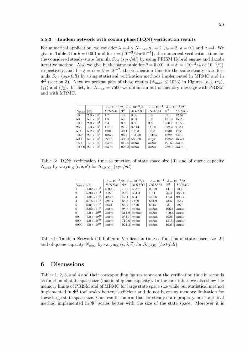
5.5.3 Tandem network with coxian phase(TQN) verification results

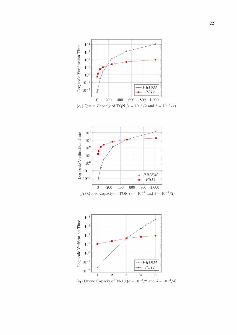
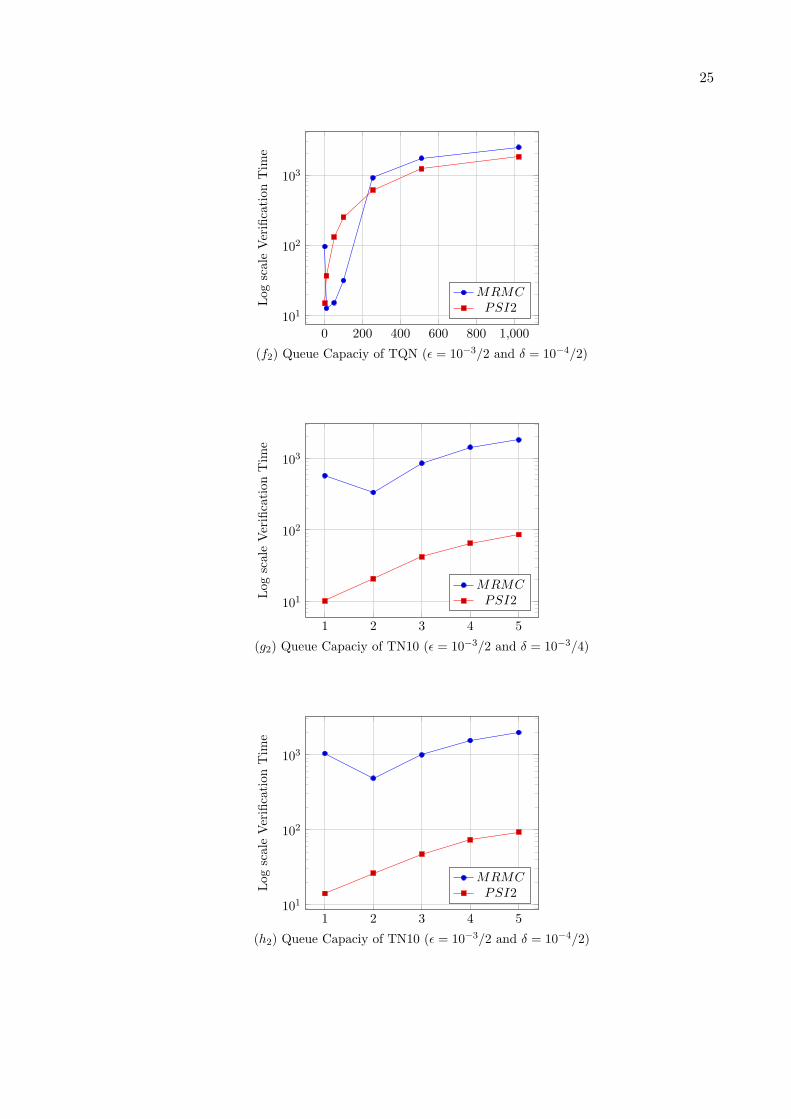
For numerical application, we consider λ = 4×Nmax, µ1 = 2, µ2 = 2, a = 0.1 and κ =4. Wegive in Table 3 for θ = 0.001 and for ǫ = {10−3/2or10−4}, the numerical verification time forthe considered steady-state formula S<θ (sys-full) by using PRISM Hybrid engine and Jacobiiterative method. Also we give in the same table for θ = 0.001, δ = δ′ = {10−3/4 or 10−4/2}respectively, and 1 − ξ = α = β = 10−2, the verification time for the same steady-state for-mula S<θ (sys-full) by using statistical verification methods implemented in MRMC and inΨ2 (section 3). Next we present part of these results (Nmax ≤ 1023) in Figures (e1), (e2),(f1) and (f2). In fact, for Nmax = 7500 we obtain an out of memory message with PRISMand with MRMC.

ǫ = 10−3/2, δ = 10−3/4 ǫ = 10−4, δ = 10−4/2Nmax |X | PRISM Ψ2 MRMC PRISM Ψ2 MRMC10 2.3 ∗ 102 1.7 1.4 0.08 1.8 37.1 12.6750 5.1 ∗ 103 1.8 5.4 0.01 1.9 131.4 15.23100 2.0 ∗ 104 3.4 9.8 0.05 3.6 250.7 31.56255 1.3 ∗ 105 117.9 24.2 32.14 119.0 612.4 912.4511 5.2 ∗ 105 1201 49.1 70.93 1208 1230 17351023 2.1 ∗ 106 10879 96.4 131.50 13105 1822 24795000 5.1 ∗ 107 itrpr 493.2 586.70 itrpr 12258 153217500 1.1 ∗ 108 outm 819.6 outm outm 19153 outm10000 2.1 ∗ 108 outm 925.3 outm outm 23219 outm

Table 3: TQN: Verification time as function of state space size |X | and of queue capacityNmax by varying (ǫ, δ, δ′) for S<0.001 (sys-full)

ǫ = 10−3/2, δ = 10−3/4 ǫ = 10−4, δ = 10−4/2Nmax |X | PRISM Ψ2 MRMC PRISM Ψ2 MRMC1 1.02 ∗ 103 0.023 10.2 553.7 0.029 14.1 10392 5.90 ∗ 104 1.27 20.9 334.4 1.31 26.4 485.13 1.04 ∗ 106 42.78 42.1 854.1 46.06 47.3 993.74 9.76 ∗ 106 591.7 65.3 1429 661.9 73.5 15475 6.04 ∗ 107 5821 86.2 1810 6315 93.1 19766 2.82 ∗ 108 outm 98.8 outm outm 196.1 outm9 1.0 ∗ 1010 outm 311.9 outme outm 619.6 outm99 1.0 ∗ 1020 outm 2311 outm outm 4926 outm999 1.0 ∗ 1030 outm 719.6 outm outm 15156 outm9999 1.0 ∗ 1040 outm 921.3 outm outm 19216 outm

Table 4: Tandem Network (10 buffers): Verification time as function of state space size |X |and of queue capacity Nmax by varying (ǫ, δ, δ′) for S<0.001 (last-full)

6 Discussions

Tables 1, 2, 3, and 4 and their corresponding figures represent the verification time in secondsas function of state space size (maximal queue capacity). In the four tables we also show thememory limits of PRISM and of MRMC for large state space size while our statistical methodimplemented in Ψ2 tool scales better, is efficient and do not have any memory limitation forthese large state space size. Our results confirm that for steady-state property, our statisticalmethod implemented in Ψ2 scales better with the size of the state space. Moreover it is

27

generally faster than the numerical method implemented in PRISM and than the statisticalmethod implemented in MRMC. However, high accuracy comes at a greater price than fornumerical method.

In fact, when comparing the efficiency of PRISM (numerical) and of Ψ2 (statistical) wefound that: For the smaller models (monotone and non-monotone cases), the PRISM toolis slightly faster. However, for the larger models (monotone and non-monotone cases), ourstatistical method implemented in Ψ2 is faster than PRISM.

When comparing the efficiency of MRMC (statistical) and of Ψ2 (statistical) and whencomparing the scalability of the three considered tools we found that: For Tandem network(4 buffers) case, Ψ2 is faster than MRMC for large state space size |X | (due to monotonicityof model), and we obtain an out of memory message in PRISM and in MRMC from the value|X | = 1.0 ∗ 108 (corresponding to Nmax = 99). For Multistage delta network case, MRMCis slightly faster for the small |X | while Ψ2 becomes faster than MRMC for large |X | (dueto the considered rare event property), and we obtain an out of memory message in PRISMand in MRMC from the value |X | = 2.1 ∗ 108 (corresponding to Nmax = 10). For Tandemnetwork with coaxian phase case, MRMC is slightly faster for the small |X | while Ψ2 becomesslightly faster than MRMC for large |X | (due to non monotonicity of model and to the smallqueue number), and we obtain an out of memory message in PRISM and in MRMC from thevalue |X | = 1.1∗108 (corresponding to Nmax = 7500). For Tandem network (10 buffers) case,Ψ2 is faster than MRMC for large |X | (due to large queue number and to rare regenerationpoints), and we obtain an out of memory message in PRISM and in MRMC from the value|X | = 2.8 ∗ 108 (corresponding to Nmax = 6).

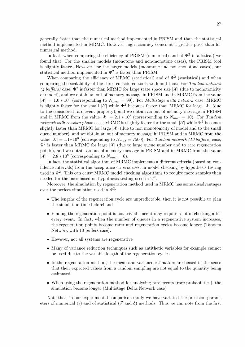
In fact, the statistical algorithm of MRMC implements a different criteria (based on con-fidence intervals) from the acceptance criteria used in model checking by hypothesis testingused in Ψ2. This can cause MRMC model checking algorithms to require more samples thanneeded for the ones based on hypothesis testing used in Ψ2.

Moreover, the simulation by regeneration method used in MRMC has some disadvantagesover the perfect simulation used in Ψ2:

• The lengths of the regeneration cycle are unpredictable, then it is not possible to planthe simulation time beforehand

• Finding the regeneration point is not trivial since it may require a lot of checking afterevery event. In fact, when the number of queues in a regenerative system increases,the regeneration points become rarer and regeneration cycles become longer (TandemNetwork with 10 buffers case).

• However, not all systems are regenerative

• Many of variance reduction techniques such as antithetic variables for example cannotbe used due to the variable length of the regeneration cycles

• In the regeneration method, the mean and variance estimators are biased in the sensethat their expected values from a random sampling are not equal to the quantity beingestimated

• When using the regeneration method for analysing rare events (rare probabilities), thesimulation become longer (Multistage Delta Network case)

Note that, in our experimental comparison study we have variated the precision param-eters of numerical (ǫ) and of statistical (δ′ and δ) methods. Thus we can note from the first

28

four tables that the numerical verification time dependence on ǫ is negligible while the sta-tistical verification time dependence on δ and on δ′ is considerable. Moreover, we refer tosection 2 to explain why in some of our case studies, the obtained statistical verification timewhen using Ψ2 does not depend on |X |. Finally, note that even if we do not use sequentialacceptance sampling which is more efficient than single one used in our statistical methodimplemented in Ψ2, we obtain more efficient and more scalable results than other methods.

7 Conclusion and future works

In this research report, we have empirically compared numerical and two different statisticalsolutions implemented in PRISM, MRMC and Ψ2 tools for probabilistic model checking oncase studies taken from the PRISM and Ψ2 benchmarks. We focused our attention on steady-state properties. For these properties, we have found that our statistical method implementedin Ψ2 scales better with the state space size and it is faster than PRISM and MRMC toolsespecially for large models. In fact, we aim to find the limiting problem sizes for the consid-ered case studies. We see that our statistical approach scales well with the problem size andit allows us to consider very large models. We see that our statistical approach scales wellwith the problem size, it is generally more efficient than the PRISM (numerical) and MRMC(statistical) approaches and it allows us to consider very large models and to verify rare eventproperties efficiently.

References

[1] J. M. Vincent A. Busic and B. Gaujal. Perfect simulation and non-monotone (marko-vian) systems. In VALUETOOLS08. ACM, 2008.

[2] C. Baier, B. Haverkort, H. Hermanns, and J.P. Katoen. Model-checking algorithms forcontinuous-time markov chains. IEEE Trans. Software Eng., 29(6):524–541, 2003.

[3] C. Baier and J. P. Katoen. Principles of Model Checking. The MIT Press, 2008.

[4] P. Fernandes, J. M. Vincent, and T. Webber. Perfect simulation of stochastic automatanetworks. In ASMTA08, volume 5055 of LNCS, pages 249–263, 2008.

[5] G. Gorgo, J.M. Vincent, and B. Gaujal. Envelope perfect sampling of phase-type serversin queueing networks. Technical report, INRIA-University of Grenoble, 2010.

[6] G. Norman H. L. S. Younes, M. Z. Kwiatkowska and D. Parker. Numerical vs. statisticalprobabilistic model checking. STTT, 8(3):216–228, 2006.

[7] T. Herault, R. Lassaigne, and S. Peyronnet. Apmc 3.0: Approximate verification of dis-crete and continuous time markov chains. In QEST06, pages 129–130. IEEE ComputerSociety, 2006.

[8] A. Hinton, M. Kwiatkowska, G. Norman, and D. Parker. Prism: A tool for automaticverification of probabilistic systems. In TACAS06, volume 3922 of LNCS, pages 441–444,2006.

[9] J. P. Katoen, I. S. Zapreev, E. M. Hahn, H. Hermanns, and D. N. Jansen. The insand outs of the probabilistic model checker mrmc. In QEST09, pages 167–176. IEEEComputer Society, 2009.

29

[10] D.A. Levin, Y. Peres, and E.L. Wilmer. Markov Chains and Mixing Times. AMS, 2009.

[11] D. Propp and J. Wilson. Exact sampling with coupled markov chains and applicationsto statistical mechanics. Random Structures and Algorithms, 9(1 and 2):223–252, 1996.

[12] D. El Rabih, G. Gorgo, N. Pekergin, and J. M. Vincent. Steady state property verifi-cation: a comparison study. In VECOS10, pages 4–15. ewic, British Computer Society,2010.

[13] D. El Rabih, G. Gorgo, N. Pekergin, and J.M. Vincent. Steady-state dependability ver-ification by perfect sampling: Comparison study. Technical report, LACL-University ofParis Est, 2010.

[14] D. El Rabih and N. Pekergin. Statistical model checking for steady state dependabilityverification. In DEPEND09, pages 166–169. IEEE Computer Society, 2009.

[15] D. El Rabih and N. Pekergin. Statistical model checking using perfect simulation. InATVA09, volume 5799 of LNCS, pages 120–134. Springer, 2009.

[16] K. Sen, M. Viswanathan, and G. Agha. Vesta: A statistical model-checker and analyzerfor probabilistic systems. In QEST05, pages 251–252. IEEE Computer Society, 2005.

[17] J. M. Vincent. Perfect simulation of monotone systems for rare event probability esti-mation. In Winter Simulation Conference, pages 528–537. ACM, 2005.

[18] J. M. Vincent and J. Vienne. ψ2 a software tool for the perfect simulation of finitequeueing networks. In QEST07, pages 113–114. IEEE Computer Society, 2007.

[19] J.M. Vincent and C. Marchand. On the exact simulation of functionals of stationarymarkov chains. Linear Algebra and its Applications, 386:285–310, 2004.

[20] H. L. S. Younes. Ymer: A statistical model checker. In CAV05, volume 3576 of LNCS,pages 429–433, 2005.

[21] H. L. S. Younes. Error control for probabilistic model checking. In VMCAI06, volume3855 of LNCS, pages 142–156, 2006.

[22] H. L. S. Younes and R. G. Simmons. Statistical probabilistic model checking with afocus on time-bounded properties. Inf. Comput., 204(9):1368–1409, 2006.