Embed Size (px)
Citation preview

arX
iv:0
810.
4832
v1 [
astr
o-ph
] 27
Oct
200
8Astronomy & Astrophysicsmanuscript no. 0137 c© ESO 2008October 27, 2008
Stellar abundances and ages for metal-rich Milky Way globul arclusters
Stellar parameters and elemental abundances for 9 HB stars in NGC 6352⋆⋆⋆
S. Feltzing1, F. Primas2, and R.A. Johnson3
1 Lund Observatory, Box 43, SE-221 00 Lund, Swedene-mail:[email protected]
2 European Southern Observatory, Karl-Schwarzschild Str. 2, 85748 Garching b. Munchen, Germanye-mail:[email protected]
3 Astrophysics, Oxford University, Denys Wilkinson Building, Keble Road, Oxford, OX1 3RH, UKe-mail:[email protected]
Received 2008-05-06; Accepted 2008-09-16
ABSTRACT
Context. Metal-rich globular clusters provide important tracers ofthe formation of our Galaxy. Moreover, and not less important,they are very important calibrators for the derivation of properties of extra-galactic metal-rich stellar populations. Nonetheless, onlya few of the metal-rich globular clusters in the Milky Way have been studied using high-resolution stellar spectra to derive elementalabundances. Additionally, Rosenberg et al. identified a small group of metal-rich globular clusters that appeared to beabout 2 billionyears younger than the bulk of the Milky Way globular clusters. However, it is unclear if like is compared with like in thisdataset aswe do not know the enhancement ofα-elements in the clusters and the amount ofα-elements is well known to influence the derivationof ages for globular clusters.Aims. To derive elemental abundances for the metal-rich globularcluster NGC 6352 and to present our methods to be used in up-coming studies of other metal-rich globular clusters.Methods. We present a study of elemental abundances forα- and iron-peak elements for nine HB stars in the metal-rich globularcluster NGC 6352. The elemental abundances are based on high-resolution, high signal-to-noise spectra obtained with the UVESspectrograph on VLT. The elemental abundances have been derived using standard LTE calculations and stellar parameters have beenderived from the spectra themselves by requiring ionizational as well as excitational equilibrium.Results. We find that NGC 6352 has [Fe/H]= −0.55, is enhanced in theα-elements to about+0.2 dex for Ca, Si, and Ti relativeto Fe. For the iron-peak elements we find solar values. Based on the spectroscopically derived stellar parameters we find that anE(B − V) = 0.24 and (m − M) ≃ 14.05 better fits the data than the nominal values. An investigation of logg f -values for suitable Feilines lead us to the conclusion that the commonly used correction to the May et al. (1974) data should not be employed.Conclusions.
Key words. (Galaxy:) globular clusters: individual:NGC 6352, Stars:horizontal-branch, Stars: abundances
1. Introduction
The globular clusters in a galaxy trace (part of) the formationhistory of their host galaxy, in particular merger events havebeen shown to trigger intense periods of formation of stellarclusters (e.g. Forbes 2006). The perhaps most spectacular ev-idence of such an event is provided by the Antennae galaxies(Whitmore & Schweizer 1995; Whitmore et al. 1999). Resultsfor the recent merger system NGC 1052/1316 appear to showthat indeed some of the clusters that form in a merger eventbetween gas-rich galaxies may result in what we today iden-tify as globular clusters (Forbes 2006; Goudfrooij et al. 2001;Pierce et al. 2005).
Send offprint requests to: S. Feltzing⋆ Based on observations collected at the European Southern
Observatory, Chile, ESO No. 69.B-0467⋆⋆ Table 3 is only available in the on-line version of the paper or inelectronic form at the CDS via anonymous ftp to cdsarc.u-strasbg.fr(130.79.128.5) or via http://cdsweb.u-strasbg.fr/cgi-bin/qcat?J/A+A/
Even though globular clusters are thought to probe importantepisodes in the formation of galaxies there is increasing evidencethat they may not be a fair representation of the underlying stellarpopulations. For example, VanDalfsen & Harris (2004) pointoutthe increasing evidence that the metallicity distributionfunctionsfor globular clusters in other galaxies less and less resemble themetallicity distribution functions of the field stars in their hostgalaxies.
Nevertheless, globular clusters provide one of the most pow-erful tools for studying the past history of galaxies outside theLocal Group and in order to fully utilize this it becomes impor-tant to find local templates that can be used to infer the propertiesof the extra-galactic clusters. Such templates can be providedby the Milky Way globular clusters and clusters in the LMCand SMC. There is a large literature on this, especially for themetal-poor clusters (i.e. for clusters with iron abundances lessthan –1 dex, see e.g. Gratton et al. 2004, and references therein).However, for the metal-rich clusters with with iron abundanceslarger than−1 dex (which are extremely important for studies

2 S. Feltzing et al.: Stellar abundances and ages for metal-rich Milky Way globular clusters
of e.g. bulges and other metal-rich components of galaxies)thesituation is less developed.
The Milky Way has around 150 globular clusters. Theseshow a bimodal distribution in colour as well as in metallic-ity (e.g. Zinn 1985). Such bimodalities are quite commonly ob-served also in other galaxies. The source of the bimodality couldbe a period of heightened star formation, perhaps triggeredby amajor merger or a close encounter with another (large) galaxy.For example, Casuso & Beckman (2006) advocates a picturewhere the metal-rich globular clusters in the Milky Way formedduring times of enhanced star formation (perhaps triggeredby aclose passing by by the LMC and/or SMC) and that some, butnot all, of these new young clusters were “expelled” to altitudesmore akin to the thick than the thin disk or that the clusters actu-ally formed at these higher altitudes. That second possibility issomewhat related to the model by Kroupa (2002) which was de-veloped to explain the scale height of the Milky Way thick disk.In contrast, VanDalfsen & Harris (2004) advocates a fairly sim-ple chemical evolution model of the “accreting-box” sort toex-plain the bimodal metallicity distribution of the globularclustersin the Milky Way. This model is able to reproduce the observedmetallicity distribution function but offers no explicit explana-tion of why the different epochs of heightened star formationhappened.
To put constraints on these types of models it thus becomesinteresting to study the age-structure for the globular clustersin the Milky Way. Rosenberg et al. (1999) found that a smallgroup of metal-rich clusters, NGC 6352, 47 Tuc, NGC 6366, andNGC 6388 (all with [Fe/H] > −0.9), show apparent young ages,around 2 Gyr younger than the bulk of the cluster system. As dis-cussed in detail in Rosenberg et al. (1999) the ages of this groupare model dependent, but, the internal consistency is remarkableand intriguing. However, it is not clear if like is compared withlike in this group of clusters. The reasons are (at least) two, firstthis group includes a mixture of disk and halo clusters, secondlyknowledge of theα-enhancement is not available for all of theclusters. In fact these concerns are connected. We know, fromthe local field dwarfs, that the chemical evolution in the halo andthe disk are different, i.e. the majority of the stars in the halohave a largeα-enhancement, while in the disk we see a declineof theα-enhancement starting somewhere around the metallici-ties of these clusters (see e.g. Bensby et al. 2005). Thus it couldwell be that the halo and disk clusters have distinct profilesasconcerns their elemental abundances. In that case the derivationof the ages of the clusters in relation to each other might be er-roneous asα-enhancement clearly affect age determinations (seee.g. Salasnich et al. 2000; Kim et al. 2002).
We have therefore constructed a program to provide a homo-geneous set of elemental abundances for a representative set ofmetal-rich globular clusters, including both halo and bulge clus-ters. The two globular clusters NGC 6352 and NGC 6366 pro-vide an unusually well-suited pair to target for a detailed abun-dance analysis. NGC 6352 is a member of thedisk cluster pop-ulation while NGC 6366, although it is metal-rich, unambigu-ously, due to its kinematics, belong to thehalopopulation.
Further, both clusters are ideal for spectroscopic studiessince they are sparsely populated. This means that it is easytoposition the slit on individual stars even in the very central partsof the cluster. 47 Tuc on the other hand is around 100 times morecrowded and spectroscopy of single stars becomes increasinglydifficult. The fourth cluster, NGC 6388, is also very centrallyconcentrated and therefore less amenable to spectroscopicstud-ies. For both NGC 6352 and NGC 6366 the background contam-
ination is minimal so that the selected horizontal branch (HB)stars should all be members.
Good colour-magnitude diagrams exist for both clusters;for NGC 6352 based on HST/WFPC2 observations and forNGC 6366 a good ground-based CMD exists (Alonso et al.1997). Combined with our new elemental abundances we wouldthus be in a position to do a relative age dating of these two clus-ters.
We have obtained spectra for nine HB stars in NGC 6352 andeight in NGC 6366. In addition we also have data for six HB andred giant branch stars (RGB) in NGC 6528 from our own obser-vations which will be combined with observations of additionalstars present in the VLT archive. Additional archival materialexist for other metal-rich globular clusters. Also for NGC 6528decent CMDs exist (e.g. Feltzing & Johnson 2002).
Here we report on the first determinations of elemental abun-dances for one of the globular clusters, NGC 6352, in the pro-gram. We also spend extra time explaining the methods that wewill use also for the other cluster, especially as concerns thechoice of atomic data for the abundance analysis.
The paper is organized as follows: in Sect. 2 we describethe selection of target stars for the spectroscopic observationsin NGC 6352. Section 3 deals with the observations, data reduc-tion and analysis of the stellar spectra. Section 4 describes in de-tail our abundance analysis, including a discussion of the atomicdata used. In Sect. 5 the elemental abundance results are pre-sented. The results are discussed in Sect. 6 in the context ofothermetal-rich globular clusters and the Milky Way stellar popula-tions in general. Section 7 provides a summary of our findings.
2. Selection of stellar sample for our spectroscopicprogramme for NGC 6532
Stars for the spectroscopic observations were selected based ontheir position in the CMD. Only a few stars in NGC 6352 havepreviously been studied with spectroscopy and hence there wasno prior knowledge of cluster membership. Therefore we de-cided to select only stars on the HB in order to maximize the pos-sibility for them to be members. Selecting HB stars rather thenRGB and AGB stars has the further advantage that the stars willhave fairly high effective temperatures (Teff) which significantlywill facilitate the analysis of the stellar spectra. At lower temper-atures the amount of molecular lines start to become rather prob-lematic (see e.g. the discussion in Barbuy 2000; Carretta etal.2001; Cohen et al. 1999).
The HB in NGC 6352 is situated atV555 ∼ 15.2. Data for thetarget stars for the spectroscopic programme are listed in Table 1.In Fig. 1 we show a mosaic image based on HST/WFPC2 imageswith the stars observed in the spectroscopic programme labeledby their corresponding numbers from Table 1. The table alsoincludes a cross-identification with designations used in othermajor studies of NGC 6352 (Alcaino 1971; Hartwick & Hesser1972).
3. Spectroscopy
3.1. Observations and data reduction
Observations were carried out in service mode as part of ob-serving programme 69.B-0467 with the UVES spectrograph onKueyen. We used the red CCD with a standard setting centeredat 580.0 nm. With this setting we cover the stellar spectra from480.0 to 680.0 nm with a gap between 576.0 nm and 583.5 nm.Each star was observed for 4800 s in a single exposure.

S. Feltzing et al.: Stellar abundances and ages for metal-rich Milky Way globular clusters 3
Table 1. Data for our sample. The first column gives our designation for the stars (compare Fig. 1), second and third give al-ternative designations of the stars from Alcaino (1971) (marked by A×××) and Hartwick & Hesser (1972) (marked by H×××).Column four and five give the stellar coordinates (taken fromthe 2MASS survey, Skrutskie et al. 2006). Columns six and sevengive the HST/WFPC2 in-flight magnitudes and colours. The last column lists theK magnitude for the stars from the 2MASS survey(Skrutskie et al. 2006).
Star A××× H××× α δ V555 V555− I814 K
NGC 6352-01 – – 261.378121 -48.425865 15.32 1.28 12.437NGC 6352-02 – H220 261.400858 -48.420418 15.34 1.33 12.181NGC 6352-03 A61 H56 261.392403 -48.428165 15.24 1.18 12.320NGC 6352-04 A58 H234 261.409088 -48.432890 15.30 1.20 12.325NGC 6352-05 A56 H237 261.405980 -48.436588 15.22 1.17 12.342NGC 6352-06 A155 H250 261.384160 -48.440037 15.28 1.16 12.445NGC 6352-07 A152 H252 261.377315 -48.441895 15.26 1.20 12.420NGC 6352-08 A151 – 261.376366 -48.443417 15.25 1.16 12.406NGC 6352-09 A150 H253 261.373965 -48.443913 15.30 1.21 12.354
Fig. 1. HST/WFPC2 mosaic image ofNGC 6352 (the PC image is excluded).The stars with UVES spectra aremarked with the corresponding num-bers from Table 1. This image is createdfrom the following three HST/WFPC2datasets: u28q0404t, u28q0405t, andu28q040bt.
The spectra were pipeline calibrated as part of the servicemode operation. As our spectra are of moderate S/N (in the redup to 80, but in the blue more like 60) we have visually inspectedthe reduced and extracted one-dimensional spectra for knownfoibles and found them to not suffer from any of these problems.
3.2. Radial velocity measurements and cluster membership
Radial velocities were measured from the stellar spectra usingtherv suite of programs insideiraf1. From the observed radialvelocities helio centric velocities and velocities relative to the
1 IRAF is distributed by National Optical Astronomy Observatories,operated by the Association of Universities for Research inAstronomy,Inc., under contract with the National Science Foundation,USA.
local standard of rest (LSR) were calculated and are listed inTable 2. We find the cluster to have a mean velocity relative tothe LSR of –120.7 km s−1 with σ = 3.7 km s−1. All of ourprogram stars have velocities that deviate less then 2σ from themean velocity. Hence they are all members.
The most recent value forVLSR in the catalogue of globularclusters (Harris 1996, catalogue2) is −116.7km s−1. This is inreasonably good agreement with our new result based on datafor nine stars. The Harris (1996) value is based on a weightedaverage from three studies (Rutledge et al. 1997; Zinn & West1984; Hesser et al. 1986). Rutledge et al. (1997) foundVHelio =
2 We have used the latest revision (2003) available athttp://www.physics.mcmaster.ca/Globular.html

4 S. Feltzing et al.: Stellar abundances and ages for metal-rich Milky Way globular clusters
Table 2. Measured and derived velocities. The second columngives the radial velocity of the star as measured from the stellarspectrum. The third column the derived helio centric velocityand the fourth the velocity relative to the local standard ofrest(LSR). The last line gives the mean helio centric velocity for allthe stars and the corresponding standard deviation as well as themean LSR velocity with its corresponding standard deviation.
Star V0bs VHelio VLSR
km s−1 km s−1 km s−1
NGC 6352-01 –154.30 –146.18 –127.36NGC 6352-02 –147.13 –142.05 –123.24NGC 6352-03 –141.65 –136.72 –117.90NGC 6352-04 –140.71 –135.87 –117.06NGC 6352-05 –144.62 –139.90 –121.09NGC 6352-06 –137.72 –133.75 –114.94NGC 6352-07 –143.60 –139.52 –120.71NGC 6352-08 –144.81 –140.63 –121.82NGC 6352-09 –148.53 –141.31 –122.50
NGC 6352 –139.5σ = 3.7 –120.7σ = 3.7
−122.8km s−1 for a sample of 23 stars. Using the followingequation
VLSR = VHelio + 11.0 cosb cosl + 14.0 cosb sinl + 7.5 sinb
(Ratnatunga et al. 1989), withl = 341.4 and b = −7.2 forNGC 6352, this corresponds to aVLSR = −117.9 km s−1. We notethat Rutledge et al. (1997) estimate their external errors for themeasurement of the radial velocities for stars in NGC 6352 tobeon the order of 10 km s−1. More recently, Carrera et al. (2007)find VHelio = −114 km s−1 based on 23 stars, which is equiva-lent to VLSR = −109 km s−1. No estimate of external errors aregiven in their study. Their value is more similar to that mea-sured by Hartwick & Hesser (1972),VHelio = −112.2km s−1,than to ours. There are no stars in common between our studyand Carrera et al. (2007)3.
Hence, it does appear that our estimate ofVLSR forNGC 6352 is somewhat high when compared to other estimatesavailable in the literature. However, as we do not have a goodes-timate of zero-point errors for the various studies and as nodoubtdifferent types of stars have been used in the various studies, e.g.we use only HB stars whilst some of the earliest studies clearlywill have relied on very cool giants where e.g. motions in thestellar atmospheres might play a role (Carney et al. 2003), andsince we have no information on binarity for any of these starsthe current value should be regarded as being in good agreementwith previous estimates.
3.3. Measurement of equivalent widths
Equivalent widths were measured using thesplot task iniraf. For each line the local continuum was estimated withthe help of synthetic spectra generated using appropriate stel-lar parameters and a line-list, typical for a K giant, fromVALD, see Piskunov et al. (1995), Ryabchikova et al. (1999),
3 We thank the authours for making the coordinates of their sampleavailable to us so that we could check for common stars. None werefound.
and Kupka et al. (1999). The equivalent widths used in the abun-dance analysis are listed in Table 34.
4. Abundance analysis
We have performed a standard Local ThermodynamicEquilibrium (LTE) analysis to derive chemical abundancesfrom the measured values ofWλ using the MARCS stellarmodel atmospheres (Gustafsson et al. 1975; Edvardsson et al.1993; Asplund et al. 1997).
When selecting spectral lines suitable for analysis in a gi-ant star spectrum we made much use of the VALD database(Kupka et al. 1999; Ryabchikova et al. 1999; Piskunov et al.1995). VALD also provided damping constants as well as termdesignations which were used in the calculation of the linebroadening.
4.1. logg f -values – general comments
The elemental abundance is, for not too strong lines, basicallyproportional to the oscillator strength (logg f ) of the line, hencecorrect logg f -values are important for the accuracy of the abun-dances. Oscillator strengths may be determined in two ways(apart from theoretical calculations) – either through measure-ments in laboratories or from a stellar, most often solar, spec-trum. The latter types of logg f -values are normally called astro-physical. The astrophysical logg f -values are determined by re-quiring the line under study to yield the, pre-known, abundanceof that element for the star used. Since the Sun is the star forwhich we have the best determined elemental abundances nor-mally a solar spectrum is used. An advantage of the astrophys-ical logg f -values is that, if the solar spectrum is taken with thesame equipment as the stellar spectra are, any irregularities inthe recorded spectrum that arise from the instrumentation andparticular model atmospheres used will, to first order, cancel.
The laboratory data have a specific value in that they al-low absolute determination of the stellar abundances. Obviouslyalso these data have associated errors and therefore one shouldexpect some line-to-line scatter in the final stellar abundances.Furthermore, the absolute scale of a set of laboratory logg f -values can be erroneous and then the resulting abundances willbe erroneous with the same systematic error as present in thelaboratory data (see e.g. our discussion as concerns the logg f -values for Cai).
We have chosen different options for different elements de-pending on the data available. Our ambition has been to createa line-list that is homogeneous for each element and which canbe used in forthcoming studies of giant stars in other globularclusters.
Whenever possible we have chosen homogeneous data setsof laboratory data. When these do not exist we have chosen be-tween different options: to use purely theoretical data (if theyexist), to use only astrophysical data, or use a combinationoflaboratory and astrophysical data. In cases when we have chosenthe last option we have always checked the consistency betweenthe two sets and in general found them to be internally consistent(see below). For each element we detail which solution we optedfor and why.
As our spectra are roughly of the same resolution as the spec-tra in Bensby et al. (2003) and we do not have our own solar
4 Table 3 only appear in the online material. Table 3 is also availablein electronic form at the CDS via anonymous ftp to cdsarc.u-strasbg.fr(130.79.128.5) or via http://cdsweb.u-strasbg.fr/cgi-bin/qcat?J/A+A/.
S. Feltzing et al.: Stellar abundances and ages for metal-rich Milky Way globular clusters 5
Fig. 2. Comparison of the logg f -values for Fei lines fromMay et al. (1974) (uncorrected) and values from other studies.• mark logg f -values for lines measured by both May et al.and O’Brian et al. (1991) and the open stars mark logg f -values for lines measured by May et al. (1974) and a com-bined data set from Bard & Kock (1994), Blackwell et al.(1979), Blackwell et al. (1982c), Blackwell et al. (1982d),andO’Brian et al. (1991). The dotted line marks the one-to-one rela-tion.
observations we decided to use astrophysical logg f -values forthese lines by Bensby et al. (2003). Their analysis is based ona solar spectrum recorded with FEROS which has a resolutioncomparable to that of our UVES spectra.
4.1.1. logg f – for individual elements
Na i To our knowledge there exist no laboratory data for thelines in our spectra, however, they can be readily calculated fromtheory. We use the theoretically calculated logg f -values fromLambert & Warner (1968) as this provides a homogeneous data-set for all our Nai lines.
Si i There exist no consistent set of logg f -values for thoseSi i lines that we are able to measure in our HB spectra. Garz(1973) provides a fairly long list of laboratory Sii logg f -valuesin the visual, however, most of the wavelength region that wehave available is not covered. Out of the 16 Sii lines we canmeasure in our spectra only 5 have logg f -values from Garz(1973). A further four lines have astrophysical logg f -valuesfrom Bensby et al. (2003). We have therefore chosen to mea-sure the remaining lines in a solar spectrum and derive our ownastrophysical logg f -values for the lines not measured by Garz(1973) in order to have two homogeneous sets of logg f -valuesand in this way reduce the line-to-line scatter. We note thattheagreement between the abundances derived from lines with Garz(1973) logg f -values compares very well with those derived us-ing astrophysical logg f -values. The mean difference betweenthe two sets for all stars is 0.03 dex. For NGC 6352-08 the dif-
ference is larger, about 0.18 dex. We have no direct explanationfor this difference.
Ca i For Ca we have decided to use the laboratory logg f -valuesfrom Smith & Raggett (1981) as this data set has a high internalconsistency. We note, however, that the absolute scale of this setof logg f -values might be in error as at least two recent studies,Bensby et al. (2003) and Chen et al. (2000), have been unableto reproduce the solar Cai abundance using these logg f -values.We note that the absolute Smith & Raggett (1981) scale is basedon the logg f -value for the line at 534.9 nm. Hence if this valueshould change in the future (as the solar analyses indicates) thenour results should simply be changed by the difference betweenthe Smith & Raggett (1981) logg f -value for this line and thenew one.
Ti i The majority of the logg f -values for Tii are laboratorydata from Blackwell et al. (1982b), Blackwell et al. (1982a),Blackwell et al. (1983), and Blackwell et al. (1986) with correc-tions according to Grevesse et al. (1989). For lines not measuredby the Oxford group we apply values from Nitz et al. (1998) andKuehne et al. (1978).
Ti ii logg f -values for Tiii are taken from Tables 1 and 3 inPickering et al. (2001). Of the 21 values 5 are from Table 3 inPickering et al. which are purely theoretical values.
Fe i Our main source for identifying suitable Fei lines has beenthe compilation by Nave et al. (1994). We note that this compila-tion, although comprehensive, does not provide a critical assess-ment of the quality of the data. Therefore, we have, wheneverpossible consulted, and referenced, the original source for thelogg f -values.
One of the most important sources for experimental logg f -values for medium strong Fei lines is the work by May et al.(1974). Commonly, following Fuhr et al. (1988), a correc-tion factor is applied to the May et al. (1974) logg f -values.However, Bensby et al. (2003) found that when the correctionfactor was applied to the May et al. data their logg f -values didresult in an overabundance for the sun of 0.12 dex. Other logg f -values did not produce such a large overabundance. In Fig. 2 weshow a non-exhaustive comparison of May et al. logg f -valuesand data from several other sources (in particular O’Brian et al.(1991) and several works by Blackwell and collaborators, seefigure text). We find that the uncorrected May et al. (1974) val-ues agree very well indeed with data from other studies. Thissupport the conclusion by Bensby et al. (2003) that the correc-tion factors should not be applied to the May et al. (1974) logg f -values. We thus use the original values from May et al. (1974).
Fe ii In order to get a homogeneous data-set we have cho-sen to use the theoretically calculated logg f -values fromRaassen & Uylings (1998). They have been shown to agreevery well with data from theferrum project, see Karlsson et al.(2001) and Nilsson et al. (2000).
Ni i We have 28 Ni lines available for abundance analysis inour spectra. For 7 of these laboratory logg f -values are availablefrom Wickliffe & Lawler (1997). For the remainder (i.e. the ma-jority) no homogeneous data set is available. We thus decided to

6 S. Feltzing et al.: Stellar abundances and ages for metal-rich Milky Way globular clusters
Fig. 3. Comparison of resulting nickel abundances for eachstar when either only lines with astrophysical logg f -values areused ([Ni/H]AstPhys) or when laboratory logg f -values are used([Ni /H]Lab). The dotted line indicates the mean difference.
follow Bensby et al. (2003) and use astrophysical logg f -valuesfor these lines.
In Fig. 3 we compare the resulting [Ni/H] values when onlyastrophysical or only laboratory logg f -values are used. The dif-ference between the two line sets is small (in the mean< 0.05dex) and will thus not influence our final conclusions in any sig-nificant way. However, they show the desirability in obtaininglarger sets of laboratory logg f -values for the analysis of stellarspectra.
Al i, Mg i, Cr i, Cr ii, and Zn i No laboratory measurements ex-ist for the lines we use for these elements and we thus use as-trophysical logg f -values based on FEROS spectra taken fromBensby et al. (2003).
4.1.2. Line broadening parameters
Collisional broadening is taken into account in the calcula-tion of the stellar abundances. The abundance program fromUppsala includes cross-sections from Anstee & O’Mara (1995),Barklem & O’Mara (1997), Barklem & O’Mara (1998) 1998),Barklem et al. (1998), and Barklem et al. (2000) for over 5000lines. In particular the abundances for all but one Cai line, allCr i lines, most of the Nii, Ti i, and Fei lines are calculated inthis fashion. At the time of our first calculations we did not havedata for the Feii lines. We thus had a chance to test the influenceon the final Fe abundances as derived from the Feii lines dueto the inclusion of the more detailed treatment for the collisionsand found it to be negligible.
For the remainder of the lines we apply the classical Unsoldapproximation for the collisional broadening and use a cor-rection term (γ6). For those few Fei lines with no cross-sections we follow Bensby et al. (2003) and take theγ6 fromSimmons & Blackwell (1982) ifχl < 2.6 eV and for lines withgreater excitation potentials we follow Chen et al. (2000) anduse a value of 1.4.
As noted by Carretta et al. (2000) the collisional dampingparameters are a concern for our Nai lines. For the lines at568.265 and 568.822 nm we use the cross sections as imple-mented in the code, whilst for the lines at 615.422 and 616.075nm we use aγ6 of 1.4. The mean difference between the two setsof lines (for an LTE analysis) is 0.14 dex. This could indicate thattheγ6 used for the two redder lines is too large, however, NLTEis an additional concern for the determination of Na abundances(see Sect. 5.3).
Table 4.Reddening estimates for NGC 6352 from the literature.
E(B-V) Ref. Comment
0.44 Alcaino (1971)0.32±0.05 Hartwick & Hesser (1972)
Hesser (1976)0.29 Mould & Bessell (1984)0.21±0.03 Fullton et al. (1995)0.33 Schlegel et al. (1998) from NEDa
a The NASA/IPAC Extragalactic Database athttp://nedwww.ipac.caltech.edu/index.html
Fig. 4. Teff – (V − I)0 calibrations from Alonso et al. (1999)(dashed line), Houdashelt et al. (2000) (solid line with×), andBessell et al. (1998) (solid line with◦). The latter for modelswith and without overshooting. The colours of our target stars inNGC 6352 are indicated by vertical lines, Table 5.
For the Sii lines we use aγ6 of 1.3.If no other information is available for the collisional broad-
ening term we follow Mackle et al. (1975) and use a value of 2.5(Mg, Al, Cr ii, Ti ii, and Zn).
4.2. Stellar parameters
4.2.1. Effective temperatures
Initial estimates of the effective temperatures (Teff) for the starswere derived using our HST/WFPC2 photometry, Table 1. Thesemagnitudes are in the in-flight HST/WFPC2 system and musttherefore be dereddened and then corrected to standard Cousinscolours before the temperature can be derived.
Estimates, from the literature, of the reddening towardsNGC 6352 are collected in Table 4. Reddening towards globu-lar clusters are often determined in relation to another clusterof similar metallicity and with a well-known, and low, redden-ing value. For NGC 6352 47 Tuc has been considered a suitable

S. Feltzing et al.: Stellar abundances and ages for metal-rich Milky Way globular clusters 7
Table 5.Stellar parameters. The first column identifies the stars (see Table 1), the second gives the colour corrected for the interstellarreddening, as described in Sect. 4.2.1. The third column gives the reddening corrected colour transfered to the standard system. Itis this value that is used to derive theTeff listed in the fourth column (T phot
eff ). Column five lists theTeff derived from spectroscopy(T spec
eff ). Column six to eight list the finally adopted logg, [Fe/H], andξt (as derived in Sect. 4.2).
Star (V − I)0,HST (V − I)0 T phot,aeff T spec
eff loggspec [Fe/H] ξt(K) (K) km s−1
NGC 6352-01 1.0257 1.0382 4706 4950 2.50 –0.55 1.40NGC 6352-02 1.0709 1.0841 4609 4900 2.30 –0.55 1.30NGC 6352-03 0.9238 0.9349 4947 5000 2.50 –0.55 1.40NGC 6352-04 0.9470 0.9585 4890 4950 2.50 –0.50 1.30NGC 6352-05 0.9164 0.9274 4966 4950 2.30 –0.60 1.40NGC 6352-06 0.9056 0.9164 4994 4950 2.30 –0.55 1.40NGC 6352-07 0.9379 0.9492 4912 5050 2.70 –0.50 1.45NGC 6352-08 0.9060 0.9169 4992 5050 2.50 –0.55 1.45NGC 6352-09 0.9566 0.9681 4866 4900 2.30 –0.60 1.40
a Based on Houdashelt et al. calibration
match based on their similar metallicities. In fact their metallic-ities might differ, such that NGC 6352 is somewhat more metal-rich. This would indicate that the reddening relative to 47 Tucis an upper limit. Fullton et al. (1995) provide the latest investi-gation of the reddening estimate based on the cluster data them-selves. Their determinations are based on WFPC1 data. Theyuse two different techniques; comparison with the RGB of 47Tuc yielded 0.22 ± 0.03 mag and solving for both metallicityand reddening, using the equations in Sarajedini (1994), yielded0.21± 0.03 mag which is their recommended value. Another re-cent estimate, from the NED database, based on the galactic ex-tinction map of Schlegel et al. (1998), is 0.33 mag (see Table4).Given that this is a more general evaluation than the study byFullton et al. (1995) we have opted for the value in the latterstudy.
Differential reddening along the line-of-sight towardsNGC 6352 has been estimated to be small. Fullton et al. (1995)find it to be less then 0.02 mag for WFPC1 CCD nos. 6–8 andless than 0.07 mag for CCD No. 5. Given the various other errorsources in the photometry: the HST/WFPC2 reddening values(see below), the transformation to standard values (Eq. 1),andthe temperature calibrations (Fig. 4) we consider the reddeningtowards NGC 6352 to be constant for all our stars.
To deredden the colours in Table 1 we used the relations inHoltzman et al. (1995) Table 12. The reddening correction inV555 − I814 corresponding toE(B − V) = 0.21 is thus 0.258,which was applied to all stars.
After correcting the magnitudes for extinction we can trans-form the in-flight magnitudes to standard colours. As we haveused the relations in Dolphin (2000) to calibrate our in-flightmagnitudes5 we also use his relations to transform our in-flightmagnitudes and colours to standard Cousins colours.
V0 = V555,0 − 0.052(V − I)0 + 0.027(V − I)20
I0 = I814,0 − 0.062(V − I)0 + 0.025(V − I)20
Where,V0, I0, and (V − I)0 are the standard magnitudes andcolours, respectively, andV555,0 andI814,0 are the dereddened in-flight magnitudes. Incidentally, for these filters the coefficients
5 We have used the most updated values that are available on A.Dolphin’s web-site at http://purcell.as.arizona.edu/wfpc2 calib/
by Dolphin are identical to those by Holtzman et al. (1995) (theirTable 7).
Solving for (V − I)0 we obtain (the other solution is un-physical)
(V − I)0 =0.99−
√
0.992 + 0.004(V555− I814)0
0.004. (1)
Eq. 1 is then used to obtain the final (V − I)0 to be used toderiveTeff.
In the literature several calibrations, both empirical andthe-oretical, of colours in terms ofTeff are available. In Fig. 4 wecompare one empirical and two theoretical calibrations. Ine.g.Houdashelt et al. (2000) a more extensive comparison is avail-able. The calibration by Alonso et al. (1999) is originally calcu-lated using colours in the Johnson system, while the calibrationsby Bessell et al. (1998) and Houdashelt et al. (2000) as well asthe HST/WFPC2 in-flight UBVRI system are in the Johnson-Cousin system. The Alonso et al. (1999) calibration was trans-formed to the Johnson-Cousin system using the relations inFernie (1983).
It is noteworthy that all three calibrations, at the coloursofour stars, agree within less than 100 K. As we have no reason tobelieve that either calibration is superior and, more importantly,our colours most likely have large errors (since the variouscali-bration steps when going from in-flight HST/WFPC2 colours tostandard colours are not too well calibrated) we choose to usethe Houdashelt et al. (2000) calibration for our starting values.In Table 5 we list the derived standard colours and theTeff fromthe Houdashelt et al. (2000) calibration.
4.2.2. The metallicity of NGC 6352
The metallicity of a globular cluster is often estimated fromthe colour magnitude diagram. Several such estimates existforNGC 6352. They are listed in Table 6.
Spectroscopy of stars as faint as those in NGC 6352 is obvi-ously difficult with smaller telescopes, however, measurementsof strong lines like the IR Caii triplet lines are useful toolsand Rutledge et al. (1997) observed 23 stars in the field ofNGC 6352. They derived a metallicity of−0.5 or −0.7 dex de-pending on which calibration for the IR Caii triplet they used.
8 S. Feltzing et al.: Stellar abundances and ages for metal-rich Milky Way globular clusters
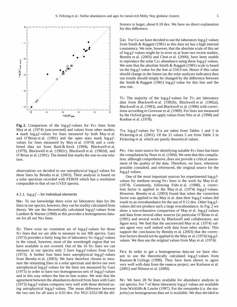
Table 6.Metallicity estimates for NGC 6352 from the literature.
[Fe/H] Method Ref. Comment
≥ 0.1± 0.1 Two-colour diagram relative to Hyades Hartwick & Hesser (1972)−1.3± 0.1 Detailed abundance analysis Geisler & Pilachowski (1981)1 star−0.3847Tuc High-resolution spectra Cohen (1983) 8 stars, 47 Tuc at−0.8 dex−0.51± 0.08 Based onQ39 Zinn & West (1984)−0.50± 0.2 TiO band strength Mould & Bessell (1984) 8 stars−0.79± 0.06 Detailed abundance analysis Gratton (1987) 3 stars−0.64± 0.06 Re-analysis ofWλ from Gratton (1987) Carretta & Gratton (1997) σ = 0.11, 3 stars−0.80 High-resolution spectra Francois (1991) 1 star
−0.50± 0.08 Caii triplet Rutledge et al. (1997) 23 stars, Based on ZW84 scalea
−0.70± 0.02 23 stars, Based on CG97 scaleb
−0.78 Re-calibration using Feiic Kraft & Ivans (2003) MARCS−0.70 Kurucz conv. overshoot−0.69 Kurucz no conv. overshoot
a ZW84= Zinn & West (1984)b CG97= Carretta & Gratton (1997).c Three different types of model atmospheres were used in the re-calibration. These are indicated in the comment column. For a full discussion
of these atmospheres as well as the results see Kraft & Ivans (2003).
Narrow-band photometry of e.g. TiO can also provide metallic-ity estimates, see e.g. Mould & Bessell (1984) who found an ironabundance of−0.50± 0.2 dex.
Detailed abundance analysis requires higher resolution andcould thus only be done for the brightest stars prior to the 8m-class telescopes. This normally means that the stars under studywill be rather cold (e.g. around 4000− 4300 K). For such coolstars detailed abundance analysis becomes harder as molecularlines become stronger when the temperature decreases. In spiteof these difficulties early studies provide interesting results fromdetailed abundance analysis. Analyzing the spectra of one starGeisler & Pilachowski (1981) derived an [Fe/H] of −1.3 ± 0.1dex while Gratton (1987) analyzed three stars and found a valueof −0.79±0.06 dex (the error being the internal error). Gratton’sWλ were later reanalyzed by Carretta & Gratton (1997) using up-dated atomic data as well as correcting the Gratton (1987)Wλs.They derived an [Fe/H] of −0.64± 0.06 dex. Cohen (1983) an-alyzed 8 stars in NGC 6352 using high-resolution spectra andfound the cluster to have a mean iron abundance of+0.38 rela-tive to 47 Tuc. With 47 Tuc at−0.8 dex this puts NGC 6352 at−0.42 dex.
Apart from the Geisler & Pilachowski (1981) value all stud-ies listed in Table 6 appear to point to an [Fe/H] for NGC 6352between−0.5 and−0.8 dex. To be perfectly sure we will ex-plore a somewhat larger range of [Fe/H] in our initial analysis(Sect. 4.2.4).
4.2.3. First estimate of logg
Assuming that the metallicities in the literature are approxi-mately correct we can use stellar evolutionary models to getan estimate of the range of surface gravities that our pro-gramme stars should have. In particular we consulted the stellarisochrones by Girardi et al. (2002) forZ = 0.001, 0.004, 0.008which corresponds to−1.33,−0.70,−0.40 dex, respectively, ac-cording to the calibration given in Bertelli et al. (1994). In thesemodels HB stars have logg between 2.2 and 2.4 dex and RGBstars at the same magnitude also have logg in this range. So evenif one or two of our stars are RGB stars (which have less redden-ing than the HB stars) exploring the same logg range will be
enough. To be entirely safe we have explored a range of loggfrom 1.7 to 2.5 dex.
4.2.4. Derivation of final stellar parameters
In this study we will assume that all the stellar parameters can bederived from the spectra themselves, what is sometimes called adetailed or fine abundance analysis. This means that we require:
– ionizational equilibrium, i.e. [Fei/H] = [Feii/H], this sets thesurface gravity,
– excitation equilibrium, that [Fei/H] as a function ofχl shouldshow no trend, this setsTeff ,
– that lines of different strengths should give the same abun-dance, i.e. [Fei/H] as a function of logW/λ should show notrend, this sets the microturbulence, and
– last but not least important, the [Fei/H] derived shouldclosely match the metallicity used to create the model at-mosphere
Often in stellar abundance analysis the investigator has a setof stellar parameters that are assumed to be rather close to the fi-nal value and a model is created with those values and the trendsdiscussed above are inspected and the parameters changed ina prescribed iterative fashion until no trends are found. Here,however, we can not be very certain about our starting values,even if we have done our best to find the most likely range(see Sect. 4.2.1, 4.2.2, and 4.2.3). Especially the reddening posesa specific uncertainty. The assumed value for the reddeningstrongly influencesTeff. We have therefore opted for a slightlydifferent approach by calculating abundances for each star for agrid of model atmospheres spanning the whole range of possiblestellar parameters. After inspecting the first grid we were thenable to refine the grid around the most likely values and producea more finely spaced grid. This grid then allowed the derivationof the stellar parameters for the final model.
First we constructed a grid of MARCS model atmospheres(Gustafsson et al. 1975, Edvardsson et al. 1993, Asplund et al.1997). The grid spans the following rangeTeff= 4500, 4600,4700, 4800, 4900, 5000, 5100 , [Fe/H]=−0.25 − 0.5,−0.75,

S. Feltzing et al.: Stellar abundances and ages for metal-rich Milky Way globular clusters 9
and logg= 1.7, 2.0, 2.3, 2.5. Using these models, the mea-sured equivalent widths and the line parameters discussed abovewe calculated Fei and Feii abundances for all models foreach star and for three different values of the microturbulence,ξt=1.0, 1.5, 2.0.This grid of results was inspected with regards tothe criteria discussed above and it turned out to be very straight-forward to identify the range of temperatures that were applica-ble. We then created a finer grid around the appropriate tempera-tures and inspected the same criteria again and from this inspec-tion it was, again, straightforward to find the stellar parametersthat fulfilled all of the criteria listed above.
An example of the final fit for NGC 6352-03 of the slopes aregiven in Fig. 5. Here we see how well the excitation and strengthcriteria are met by the set of final parameters.
In the ideal situation the four criteria listed at the be-ginning of this section should be “perfectly” met. In prac-tice we assumed that ionizational equilibrium was met when|[Fei/H]−[Feii/H]| < 0.025, that the excitation equilibrium wasachieved when the absolute value of the slope in the [Fei/H] vsχl diagram was≤ 0.005. Similarly, that theξt was found whenthe slope in the [Fei/H] vs logW/λ diagram was≤ 0.005. Forsome stars we relaxed the criterion for the absolute value oftheslope in the [Fei/H] vs χl diagram somewhat as it proved impos-sible to satisfy that at the same time as satisfying the criterionfor line strength equilibria. The final slopes are listed in Table 7and the values for [Fei/H] and [Feii/H] can be found in Table 10.We note that with the method adopted here we did only find onecombination of stellar parameters that fulfilled all four ofourcriteria, no degeneracies were found.
4.2.5. A new reddening estimate and final loggs – discussion
New reddening estimate As discussed in Sect. 4.2 and summa-rized in Table 4 the reddening estimates vary quite considerablybetween different studies. We used the reddening to derive de-reddened colours used to determineTeff in Sect. 4.2 but thesewere merely used as starting values and we subsequently foundnewTeffs. The difference between the first estimates and the fi-nal, adoptedTeff is around+90 K. We may use this temperatureoffset to derive a new estimate for the reddening. The new red-dening estimate is found by changing the reddening such thatwe minimize the difference between our spectroscopicTeff andthe photometricTeff. We find a minimum difference of 0± 20 Kif we add a further 0.036 mag to the reddening as measured inthe HST/WFPC2 in-flight system, which we found in Sect. 4.2.1to be 0.258. ThusE(V555− I814) = 0.294 which corresponds toE(B − V) = 0.24.
Surface gravity (logg) We note that although we allow logg tovary freely we did indeed, by requiring ionizational equilibrium,derive final logg values that are consistent with stellar evolution-ary tracks (e.g. Girardi et al. 2002).
NGC 6352-07 appears to have an unusually large logg forbeing situated on the HB. From its location in the CMD the starappears as a bona fide HB star (unless the reddening towardsthis particular star is significantly less than towards the stars ingeneral). The reason for this is not clear to us.
As an additional test we have used infraredK magnitudesfrom the 2MASS survey (Skrutskie et al. 2006) and the basicformula loggstar = 4.44+ 4 logTstar/T⊙ + 0.4(Mbol,star− Mbol,⊙)to estimate the loggs. For the Sun we adopted a temperatureof 5770 K andMbol,⊙ = 4.75. For the stars we used a mass of0.8 M⊙ and theTeff from Table 5. When infrared data are avail-
Fig. 5.Diagnostic check that the final parameters for NGC 6352-03 give no trends for [Fe/H] as a function ofχl and logW/λ.Parameters used to create the model atmosphere are indicatedon the top. Aξt = 1.40 was used when deriving the stellar abun-dances. The mean [Fe/H] is indicated with a dotted line in eachpanel and the trends of [Fe/H] vs χl and logW/λ are indicatedwith full lines (the dotted and full lines almost completelyover-lap). The slopes are: vsχl −0.0037 and vs logW/λ +0.0077
Table 7. Slopes for [Fe/H] for individual lines as a function ofχl and logW/λ, compare Fig. 5
Star Slope(χl) Slope(logW/λ)
NGC 6352-01 –0.0026 –0.0265NGC 6352-02 0.0002 0.0062NGC 6352-03 –0.0037 0.0077NGC 6352-04 –0.0066 –0.0225NGC 6352-05 –0.0001 0.0120NGC 6352-06 –0.0041 0.0140NGC 6352-07 –0.0059 –0.0400NGC 6352-08 –0.0023 –0.0040NGC 6352-09 0.0081 0.0068
able they are a better choice for deriving the bolometric magni-tude than the visual data as they suffer less from reddening andmetallicity effects. The bolometric magnitudes were derived us-ing Mbol = MK + BCK , where the bolometric correction was setto 1.83 (from Houdashelt et al. 2000). Using this procedure wefound a logg around 2 for all our stars withE(B − V) = 0.21and (m − M) = 14.44 (Harris 1996). However, as shown aboveour spectroscopically derivedTeffs appear to indicate a higherreddening,∼ 0.24. We also note that the error on the distancemodulus is±0.15 magnitudes (Fullton et al. 1995). Changing(m − M) to 14.05 and adopting our new reddening estimate wederive loggs of∼ 2.2 dex. However, as discussed in Sect. 4.3 andsummarized in Tables 8 and 9, the effect on the final elementalabundances from such a small change in logg is negligible.
We may thus conclude that the loggs derived by requiringionizational equilibrium for Fe is a valid method for abundanceanalysis of the type of stars studied here.

10 S. Feltzing et al.: Stellar abundances and ages for metal-rich Milky Way globular clusters
Table 8. Error estimates for NGC 6352–03. Investigation of the effect on the resulting abundances from changes of the stellarparameters. Here we changeTeff with −100 K, logg with +0.4 dex, [Fe/H] with +0.1 dex andξt with ±0.20 km s−1. The elementalabundances are given as [X/H], where X is the element indicated in the first column. For three elements we also include datafor abundances derived from lines arising from singly ionized atoms (as indicated in the first column). The second columngivesthe final elemental abundances as reported in Table 10. Here also the oneσ (standard deviation) and the number of lines used areindicated. The following columns report the changes in the abundances relative to the results reported in column two when the stellarparameters are varied as indicated in the table header. The differences are given in the sense [X/H]Final − [X/H]Modified = ∆[X/H]and [X/Fe]Final − [X/Fe]Modified = ∆[X/Fe], respectively, where X is any element. Hence the values for the modified models areequal to [X/H]Final + ∆[X/H] and [X/Fe]Final + ∆[X/Fe], respectively.
Element Final abundances ∆[X /H] ∆[X /Fe]∆Teff ∆ logg ∆[Fe/H] ∆ξt ∆Teff ∆ logg ∆[Fe/H] ∆ξt
–100K +0.4 +0.1 +0.2 –0.2 –100K +0.4 +0.1 +0.2 –0.2
Na –0.16± 0.14 (4) +0.07 +0.05 –0.01 +0.03 –0.05 –0.02 +0.04 –0.01 –0.04 +0.01Mg –0.08 (1) +0.08 +0.07 –0.01 +0.06 –0.06 –0.01 +0.06 –0.01 –0.01 0.00Al –0.11± 0.01 (2) +0.06 +0.01 0.00 +0.01 –0.02 –0.03 0.00 0.00 –0.06 +0.04Si –0.36± 0.16 (11) +0.00 –0.05 –0.01 +0.02 –0.02 –0.09 –0.05 –0.01 –0.05 +0.04Ca –0.39± 0.08 (12) +0.10 +0.05 0.00 +0.09 –0.08 +0.01 +0.04 0.00 +0.02 –0.02Ti –0.39± 0.15 (40) +0.14 +0.02 0.00 +0.06 –0.06 +0.05 +0.01 0.00 –0.01 0.00Tiii –0.24± 0.17 (14) –0.01 –0.15 –0.03 +0.08 –0.08 –0.10 –0.16 –0.03 +0.02 –0.02Cr –0.61± 0.11 (6) +0.14 +0.02 0.00 +0.07 –0.07 +0.05 +0.01 0.00 0.00 –0.01Crii –0.53± 0.15 (6) –0.05 –0.16 –0.02 +0.04 –0.04 –0.14 –0.17 –0.02 –0.03 +0.02Fe –0.54± 0.16 (193) +0.09 +0.01 0.00 +0.07 –0.06Feii –0.55± 0.11 (18) –0.07 –0.19 –0.05 –0.08+0.04 –0.17 –0.20 –0.05 –0.14 +0.11Ni –0.60± 0.10 (26) +0.07 –0.03 –0.01 +0.05 –0.06 –0.02 –0.04 –0.01 –0.02 0.00Zn –0.22± 0.05 (2) –0.03 –0.08 –0.02 +0.07 –0.07 –0.12 –0.09 –0.02 0.00 –0.01
Table 9.Slopes for NGC 6352-03 for [Fe/H] for individual linesas a function ofχl and logW/λ for the same changes in stellarparameters as in Table 8
Parameter Change Slope (χl ) Slope (logW/λ)
Final slopes –0.0037 +0.0077
∆Teff –100 K +0.0229 –0.0356∆ logg +0.4 dex –0.0029 –0.0625∆[Fe/H] +0.1 dex –0.0042 +0.0123∆ξt +0.2 km s−1 +0.0162 –0.1466
–0.2 km s−1 –0.0237 +0.1620
4.3. Stellar abundances - error budget
To investigate the effect of erroneous stellar parameters on thederived elemental abundances we have for one star, NGC 6352-03, varied the stellar parameters and re-derived the elementalabundances. The results are presented in Table 8. Note that theNa abundances reported in this table have not been correctedforNLTE effects (see Sect. 5.3)
We see that, for lines from neutral elements, errors in thetemperature scale are in general the largest error source, whilstchanges in logg generally causes smaller changes. The oppo-site is true for abundances derived from lines arising from singlyionized species.
It is notable that an error in the temperature causes essen-tially the same error in e.g. the Ca abundance as in the Fe abun-dance (from neutral lines). This means that the ratio of Ca toFeremains constant. It is also interesting to note that the Si abun-dance appears particularly robust against any erroneous param-eter. Changes in metallicity in the model cause neglible changesin the final abundances.
In Table 9 we list the slopes for the diagnostic checks forexcitation equilibrium and line strength equilibrium (compare
Fig.5 and Table 7) for each of the models used to calculate theerror estimates in Table 8. As can be seen changes inTeff as wellas inξt causes notable changes and these models would henceeasily be discarded as not fulfilling the prerequisite for a goodfit. Changes in logg and [Fe/H] causes smaller changes in theslopes. However, as can be seen in Table 8 a change in loggcauses a real change in the ionizational equilibrium and sucha model would also thus be discarded. Finally, even though achange in [Fe/H] in the model has very limited effect on slopesas well as on (most) derived elemental abundances, we requirethe model to have a [Fe/H] that is the same as that derived usingthe final model. Hence, also models with offset [Fe/H] would bediscarded.
In summary, these final considerations show that we havederived model parameters that are self-consistent and thaterrorsin [X /Fe], where X is any element, are reasonably robust againsterrors in the adopted parameters (with the exception of singlyionized species and Zn, which all have at least one change in aparameter causing a change in abundance larger than 0.1 dex.Table 8).
Additionally, we note that our internal line-to-line scatter (σ)is on par with what is found in other studies of HB and RGB starsin metal-rich globular and open clusters (e.g. Sestito et al. 2007,Carretta et al. 2001, Carretta et al. 2007, and clusters listed inTable 12).
5. Results
We have derived elemental abundances for 9 horizontal branchstars in NGC 6352. Our results are reported in Table 10 andFigs. 6 and 7.
All our abundances have been determined based on a 1DLTE analysis, though we did check the most up-to-date refer-ences on NLTE studies of all the elements investigated here.When relevant, a note has been added in the discussion below,but we note that most of the NLTE investigations have been car-

S. Feltzing et al.: Stellar abundances and ages for metal-rich Milky Way globular clusters 11
Table 10.Stellar abundances. For each star we give the mean abundance([X /H], X being the element indicated in the first column),theσ and the number of lines used in the final abundance derivation. The error in the mean is thusσ divided by
√Nlines. In the two
last entries we give the mean and median values for the cluster. For the mean value we also give theσ. The mean and median valuesare based on all nine stars.
El NGC 6352-01 NGC 6352-02 NGC 6352-03 NGC 6352-04 NGC 6352-05 NGC 6352-06
Na I –0.46 0.05 4 –0.38 0.15 4 –0.16 0.14 4 –0.49 0.12 4 –0.16 0.09 4 –0.51 0.09 4Mg I –0.18 0.00 1 –0.04 0.00 1 –0.08 0.00 1 –0.07 0.00 1 –0.09 0.00 1 –0.07 0.00 1Al I –0.22 0.21 2 –0.24 0.11 2 –0.11 0.01 2 –0.30 0.00 1 –0.30 0.23 2 –0.22 0.08 2Si I –0.31 0.13 13 –0.28 0.11 13 –0.36 0.16 11 –0.34 0.15 13 –0.40 0.14 12 –0.41 0.15 11Ca I –0.35 0.12 13 –0.19 0.11 12 –0.39 0.08 12 –0.36 0.10 12 –0.42 0.08 11 –0.40 0.11 12Ti I –0.40 0.14 35 –0.40 0.17 38 –0.39 0.15 40 –0.31 0.16 36 –0.45 0.13 36 –0.44 0.15 38Ti II –0.21 0.14 16 –0.27 0.16 15 –0.24 0.17 14 –0.09 0.39 16 –0.30 0.37 15 –0.23 0.39 16Cr I –0.59 0.11 8 –0.55 0.18 7 –0.61 0.11 6 –0.60 0.15 8 –0.70 0.07 7 –0.69 0.09 7Cr II –0.53 0.06 6 –0.56 0.12 4 –0.53 0.15 6 –0.54 0.12 3 –0.63 0.07 6 –0.70 0.16 4Fe I –0.53 0.17 201 –0.54 0.16 193 –0.54 0.16 193 –0.51 0.17 191–0.60 0.15 194 –0.57 0.16 196Fe II –0.54 0.09 18 –0.55 0.11 16 –0.55 0.11 18 –0.51 0.14 17 –0.58 0.10 17 –0.59 0.10 19Ni I –0.54 0.24 28 –0.46 0.23 28 –0.60 0.10 27 –0.57 0.11 27 –0.65 0.09 28 –0.65 0.09 26Zn I –0.21 0.17 2 –0.07 0.45 2 –0.22 0.05 2 –0.29 0.40 2 –0.49 0.00 1 –0.43 0.24 2
El NGC 6352-07 NGC 6352-08 NGC 6352-09 NGC 6352-mean NGC 6352-median
Na I –0.48 0.06 4 –0.27 0.05 4 –0.46 0.10 4 –0.37 0.14 –0.46Mg I –0.09 0.00 1 –0.03 0.00 1 –0.07 0.00 1 –0.08 0.05 –0.07Al I –0.22 0.04 2 –0.29 0.00 1 –0.16 0.00 1 –0.23 0.06 –0.22Si I –0.30 0.06 12 –0.42 0.20 12 –0.31 0.11 12 –0.35 0.05 –0.34Ca I –0.38 0.05 11 –0.38 0.09 12 –0.38 0.11 12 –0.36 0.07 –0.38Ti I –0.34 0.13 38 –0.42 0.15 36 –0.42 0.14 38 –0.40 0.05 –0.40Ti II –0.08 0.37 16 –0.16 0.38 14 –0.20 0.41 15 –0.20 0.08 –0.21Cr I –0.58 0.16 7 –0.65 0.10 7 –0.64 0.12 7 –0.62 0.05 –0.61Cr II –0.45 0.07 5 –0.64 0.08 4 –0.69 0.11 6 –0.59 0.08 –0.56Fe I –0.53 0.17 201 –0.55 0.17 196 –0.57 0.18 197 –0.55 0.03 –0.54Fe II –0.54 0.09 18 –0.56 0.10 17 –0.59 0.11 18 –0.55 0.03 –0.55Ni I –0.57 0.14 26 –0.65 0.11 26 –0.61 0.09 26 –0.59 0.06 –0.60Zn I –0.27 0.03 2 –0.45 0.16 2 –0.28 0.04 2 –0.30 0.13 –0.28
ried out for solar-type dwarf stars, hence they rarely covertheparameter space spanned by our stars.
5.1. Results – Fe, Ni and other iron-peak elements
The mean iron abundance for NGC 6352 (relative to the Sun)is −0.55± 0.03 dex. Although it is thought that Fei lines suf-fer from NLTE effects (e.g. Collet et al. 2005; Thevenin & Idiart1999), the magnitude of these effects are not yet fully estab-lished. Opposing results (very small or very large effects) havebeen found by different authors, even when studying the sameobjects. NLTE effects are expected to be of the order of 0.05 dexin stars like the Sun, and possibly increase at low metallicitiesand gravities. Feii lines remain the safest solution, but since wehave imposed the ionization balance in order to derive logg forour stars, our metallicity scale has not been corrected for anynon-LTE effect.
Ni appears somewhat under-abundant compared to iron at[Ni /Fe]= −0.04, and also Cr is slightly less abundant than ironat [Cr/Fe]= −0.07. Both results are very compatible with what isseen for local field dwarf stars at the same [Fe/H], one example isgiven by Bensby et al. (2005), as well as with results for galacticbulge stars (see Sect. 5.4).
NGC 6352-02 has a higher [Ni/H] abundance than the restof the stars and NGC 6352-01 and NGC 6352-02 have a higherline-to-line scatter. We have few direct explanations for these re-sults, although it is expected that the scatter in general should in-crease as we go to cooler stars (Luck & Heiter 2007, their Fig.1)and NGC 6352-02 is our coolest star and NGC 6352-01 one of
the cooler ones. It is also true that NGC 6352-02 has the largestscatter in Crii abundances too.
Zn shows large error-bars. We note that Bensby et al. (2003)found that, for dwarf stars more metal-rich than the sun, oneofthe lines started to give higher and higher Zn abundances whilethe other line gave lower values. The reason for this is not clearbut could have to do with that either the line is blended or thatthe line experience non-LTE effects as it gets stronger. In the HBstars the line is rather strong (75− 100 mÅ).
As reported by Asplund (2005), no NLTE analyses for iron-peak elements (except iron) have been published so far.
5.2. Results – α-elements
The cluster is clearly enhanced in theα-elements; for Si andCa the enhancement is around 0.2 dex relative to iron, (Fig. 7),while Ti is somewhat less enhanced and Mg is more enhanced.The [Mg/Fe] should be taken with a pinch of salt as we haveonly been able to measure one line and that line, although cleanand in a nice spectral region, is fairly strong in the HB stars(112–118 mÅ). Nevertheless, these enhancements are typical fordwarf stars in the solar neighbourhood that belong to the thickdisk and for galactic bulge stars (see Sect. 5.4).
We note that [Ca/H] for star NGC 6352-02 deviates substan-tially from those of the other stars. It appears that the differenceis real as we can not attribute it to e.g. continuum placementorsignificantly different stellar parameters. We include this star inour mean abundance for the cluster. If this star was excludedthe

12 S. Feltzing et al.: Stellar abundances and ages for metal-rich Milky Way globular clusters
Fig. 6.Elemental abundances for individual stars. On they-axes we show [X/H], where X is the element indicated in the upper lefthand corner in each plot. On thex-axes are the ID numbers of the stars (as defined in Table 1). For each star we also plot the errorin the mean as an error-bar. For Na we also show the NLTE corrected data (Table 1) as×. For Mg we have only analyzed one line,hence no error-bar. The same is true for three stars as concerns Al. For each element we indicate the cluster mean with a solid lineand the associatedσ (based on the values for all nine stars) with a dashed line above and below (see Table 10, penultimate column).
Fig. 7.Elemental abundances for the globular cluster NGC 6352.• with error bars indicate the mean abundance for the clusterwith it’s associated scatter (see Table 10). The dashed, horizontalline indicate the mean [Fe/H] value for the cluster stars. For eachelement we also plot the abundances using a so called box-plot.In the boxplots the central vertical line represents the medianvalue. The lower and upper quartiles are represented by the outeredges of the boxes, i.e. the box encloses 50% of the sample.The whiskers extend to the farthest data point that lies within1.5 times the inter-quartile distance. Those stars that do not fallwithin the reach of the whiskers are regarded as outliers andaremarked by dots.
Table 11.NLTE-corrected Na abundances. See Sect. 5.3 for de-tails of the correction. The first column identifies the starsac-cording to Table 1. Column two and three gives the uncorrectedNa abundances and those corrected for NLTE, respectively. Thelast column gives theσ.
Star [Na/H] [Na/H] σ
Uncorrected NLTE corrected
NGC 6352-01 –0.46 –0.60 0.04NGC 6352-02 –0.38 –0.52 0.13NGC 6352-03 –0.15 –0.30 0.12NGC 6352-04 –0.49 –0.63 0.10NGC 6352-05 –0.15 –0.30 0.07NGC 6352-06 –0.50 –0.65 0.07NGC 6352-07 –0.47 –0.62 0.04NGC 6352-08 –0.26 –0.41 0.03NGC 6352-09 –0.46 –0.60 0.08
resulting abundance would be [Ca/H]= −0.38± 0.02 as com-pared with−0.36± 0.07 if it is included.
Among these threeα-elements, only the abundances of mag-nesium could be corrected for non-LTE effects, which for mostlines are positive (in the range 0.1–0.2 dex going from the Sunto metal-poor stars). However, Asplund et al. (2005) mentions aminor dependence of the non-LTE effects on the effective tem-perature and gravity, which in turn means that the abundancesof our stars should have relatively small corrections. Correctionsfor Si are expected to be negligible, and the situation of Ca ishighly uncertain.
5.3. Results – Na and Al
Na is represented by four lines in each stellar spectrum, whilstAl is represented by two lines in most of the stars (Table 3 and10).
S. Feltzing et al.: Stellar abundances and ages for metal-rich Milky Way globular clusters 13
Both Al and Na (as well as O) are known to vary from star tostar in globular clusters (see e.g. review by Gratton et al. 2004).In fact, for RGB stars several clusters show correlations betweenAl and Na abundances (see e.g. Fig. 14 in Ramırez & Cohen2002, for a compilation of several, mainly metal-poor, globu-lar clusters) such that as [Al/Fe] increases so does [Na/Fe]. Theinterpretation of this result is complicated due to the factthatboth elements are subject to NLTE effects, although the effect islargest at low metallicities.
For Na, different studies (Baumuller et al. 1998;Mashonkina et al. 2000; Takeda et al. 2003; Shi et al. 2004) findvery similar results: non-LTE effects are stronger for warm,metal-poor stars and for low gravity stars, and they dependon the lines employed in the analysis. The smallest NLTEcorrections apply to the Nai doublet at 615.4 and 616.0 nm(corrections are less than 0.1 dex for disk stars), and to thedoublet at 568.2 and 568.8 nm (a correction of≈0.1 dex fordwarfs, though the correction seem to increase for sub-giants).Mashonkina et al. (2000) have studied the statistical equilibriumof Nai lines for a large range of stellar parameters, includingthe ones characteristic of our sample. Hence, for Na, we arein the position to be able to correct our Na abundances witha certain confidence. Based on Fig. 6 of Mashonkina et al.(2000), we have estimated non-LTE corrections of the order of−0.12 dex for the 615.4/616.0 nm doublet and of−0.16 dexfor the abundances derived from the 568.4/568.8 nm doublet.We list the revised Na abundances in Table 11 and in Fig. 6 (Napanel) we show both sets of results.
For Al, instead, the situation is not as clear as for Na.According to Baumuller & Gehren (1997), non-LTE effects forthe excited lines at 669.6/669.8 nm (the ones we have used inthis analysis) are smaller than for the Al resonance lines, butthey increase with decreasing metallicity, and they are thehigh-est at low gravities. Unfortunately, no study of NLTE in Al hasyet included mildly metal-poor giant stars, hence it is verydif-ficult to apply any correction to our abundances. In Table 2 ofBaumuller & Gehren (1997), the coolest and lowest gravity ob-ject for which non-LTE effects for the excited lines have beencomputed and found to be around+0.1 dex is a star with ef-fective temperature of 5630 K, logg = 3.08, and [Fe/H]=−0.18.Because of these uncertainties, we have decided to discuss bothNa and Al as derived from our 1D LTE analysis, and only showwhat would change in the [Na/Fe] vs. [Fe/H] diagram should weapply the corrections discussed above.
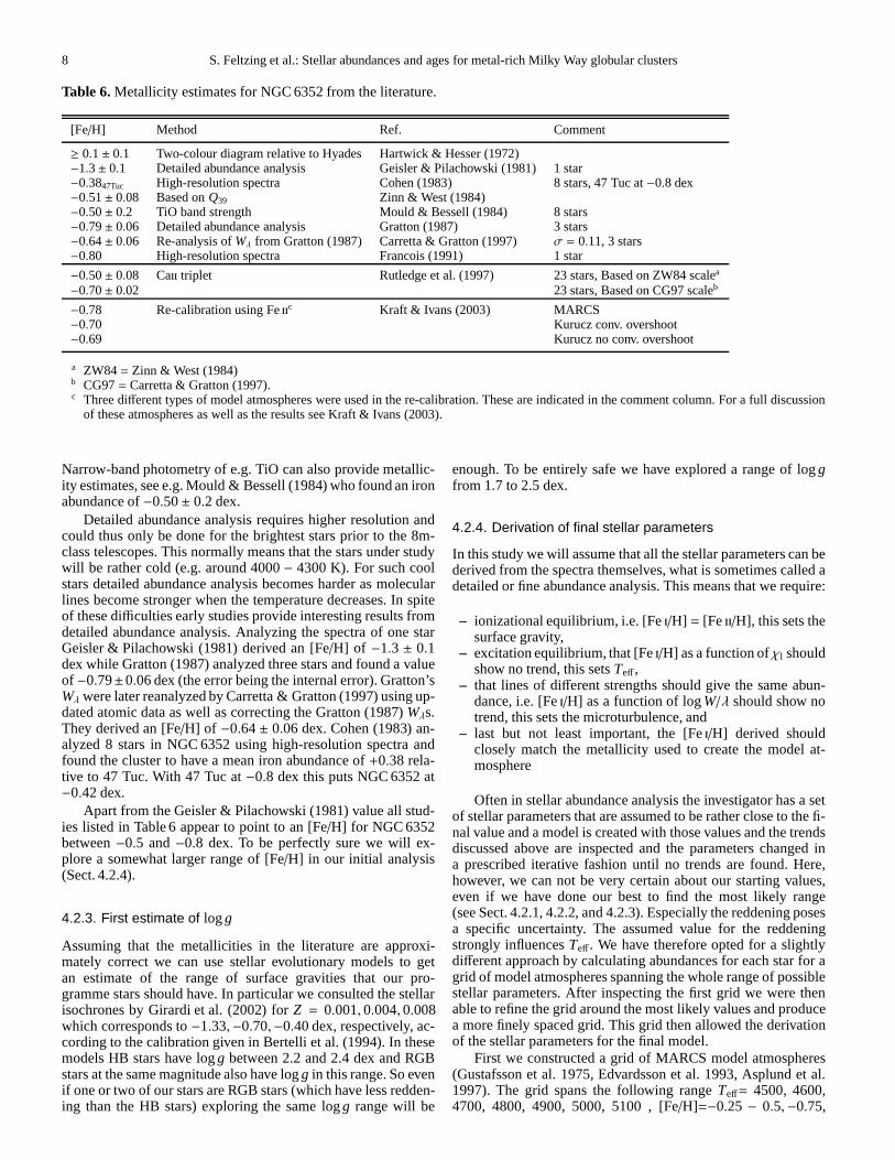
In Fig. 8 we show our [Al/Fe] vs. [Na/Fe] and compare themto those of Ramırez & Cohen (2002) for the globular clustersM 71 and M 4 (taken from Ramırez & Cohen 2002). M 71 issimilar to NGC 6352 in that it has an intermediate metallicity([Fe/H]=–0.71, Ramırez & Cohen (2002). M 4 is a metal-poorcluster (at –1.18 dex, Harris 1996). The data used to derivethe relation for M 71 included one HB star, the rest are RGBstars, both above and below the HB. Hence the comparison maybe somewhat unfair. Nevertheless we find that NGC 6352 ap-pears more enhanced in Al than M 71 and less enhanced in Nabut the slope of the correlation is similar. NGC 6352 falls be-low the trend of M 4. Both M 71 and M 4 are less metal-richthan NGC 6352. All data in Fig. 8 is without NLTE corrections.Hence, there are additional problems with this comparison inthat different types of stars (RGB vs HB) would have differentcorrections thanks to their differentTeff .
We can conclude that it appears that our data indicate thatalso on the HB there is a trend in Al and Na abundances, andthat, in metal-rich globular clusters, these correlate in amanner
Fig. 8. [Al /Fe] vs. [Na/Fe] for our stars. The dashed line indi-cates the relation found by Ramırez & Cohen (2002) for M 71.The dotted line is also taken from that paper and representthe correlation for M 4. Error-bars are shown for all stars for[Na/Fe]. Three stars only have one Al line measured. These donot have errorbars for [Al/Fe].
similar to that found for stars on the RGB in other globular clus-ters.
5.4. Comparison of elemental abundances with results fromprevious studies
In Fig. 9 we compare our abundances relative to Fe withthose derived by Geisler & Pilachowski (1981), Gratton (1987),and Francois (1991). The relative measure of [Element/Fe]should be more robust against erroneous model parameters than[Element/H] (see Table 8). Geisler & Pilachowski (1981) ana-lyzed the spectrum of one star (H37). The Geisler & Pilachowskistar was found to have an effective temperature of 4200 K, a loggof 0.9 dex, and [Fe/H]=−1.3± 0.1. Their abundances agree wellwith ours for Cr and Ni and reasonably well for Ca and Ti whilethe lighter elements differs significantly. This is probably mainlydue to the small number of lines available for those elementsin the study by Geisler & Pilachowski (1981) which means thatan error inWλ and/or logg f -value for a single line will have alarger impact than when many lines are available. We note thattheir [Fe/H] differs significantly from ours. The material avail-able in the literature does not allow a deeper investigationof thisdiscrepancy.
Gratton (1987) analyzed spectra of five metal-rich globularclusters. He analyzed spectra of three NGC 6352 stars and de-rived a mean [Fe/H] of −0.79 dex. Rutledge et al. (1997) laterconfirmed the cluster membership for two of these stars (H111and H142). Carretta & Gratton (1997) later reanalyzed the starsmeasured by Gratton (1987). ComparingWλs from their newand old spectra (for a few of the clusters where such materialwas available) they concluded that theWλs in Gratton (1987)were overestimated and derived a correction formula. Usingthe

14 S. Feltzing et al.: Stellar abundances and ages for metal-rich Milky Way globular clusters
Fig. 9.Comparison of our abundances (•) with those derived byGeisler & Pilachowski (1981) (◦) and Gratton (1987) (×), andFrancois (1991) (∗). The Gratton (1987) abundances have beencorrected, see Sect. 5.4. Error bars on our data indicate thestar-to-star scatter while those on the Geisler & Pilachowski (1981)data indicate their quoted total errors. There are no error barsavailable for the two other data sets.
correctWλ they derived an [Fe/H] of −0.64 dex. They only re-analyzed the Fei lines from Gratton (1987). As Gratton (1987)did not measure any Feii lines we are not in a position to re-analyse his data using our method as described in Sect. 4.2.4as that requires ionizational equilibrium. Instead we havede-rived a scaling of the abundances in Gratton (1987) using thestrength of the tabulatedWλs in his Table 6 using Eq. (1) inCarretta & Gratton (1997). Note that this equationis valid forNGC 6352 as it has essentially the same metallicity as Arcturus(see their discussion). The applied corrections are essentially+0.1 dex for all the elements apart from Sii which has a correc-tion of+0.2 dex. This is due to that Sii is represented by weakerlines for which the correction is larger.
In Fig. 9 we compare our data with the data from Gratton(1987) corrected as described above. For some elements, e.g.Mg, Si, and Ti, the data for his three stars agree very wellwith each other while for other elements, notably Ca and Cr,one of the stars deviates significantly from the two other stars.Comparing with our data the agreement is very good for Ca andSi but less good for the lighter elements, i.e. Mg. We also notethat there is a large discrepancy between the Cr and Ti abun-dances from the two studies. As before most of this is likely at-tributable to the few lines available for the light elementsand forCr (in Gratton only one line, we use six lines). We are more con-cerned about the discrepancy between the Ti abundances. Onepossible explanation could be the different treatment we use forthe collisional broadening.
Francois (1991) derived elemental abundances for six giantstars in three globular clusters (four stars in NGC 1904 and onestar in NGC 5927 and NGC 6352, respectively). The compari-son with our data (Fig. 9) shows an overall agreement in that
α-elements are enhanced while iron group elements are solar.There is one notable difference: Si. There is not enough infor-mation available to further investigate this discrepancy.
Overall we find that the agreement between our results andresults from earlier investigations is remarkably good consid-ering the difficulties facing the study of faint, metal-rich starsin globular clusters. This compassion further strengthensourconfidence in our abundance analysis and the conclusions thatNGC 6352 is clearly enhanced in [α/Fe] and have roughly solar[Cr/Fe] and [Ni/Fe].
6. Discussion – putting NGC 6352 into context
We now attempt a first comparison of the elemental abundanceswe find in NGC 6352 with those in other globular clusters as wellas for stars in the field (solar neighbourhood and the GalacticBulge). Our selection of comparison clusters is outlined belowand then follows a brief discussion putting NGC 6352 into con-text.
6.1. Selection of studies of other metal-rich globular clustersto compare NGC 6352 with
When compiling stellar abundances from different studies thereare a number of considerations to take into account. For giantstars there are two main issues that stands out:a) increasingimportance of molecular lines in the stellar spectra as the starsget cooler (Fulbright et al. 2006), andb) the need to include thesphericity of the stars in the calculation of model atmospheresand elemental abundances (Heiter & Eriksson 2006).
In our study of NGC 6352 we have only included HB stars toavoid the issue of molecular lines (as they are warmer than theRGB stars). HB stars are also in the region where plane paral-lel stellar models can be used (Heiter & Eriksson 2006). A firstconsideration would therefore be to only compare our elementalabundances with those of other studies of HB stars in globu-lar clusters. This, it turns out, is however, rather limiting as fewstudies have focused on HB stars.
An additional concern when selecting studies to comparewith is the different methods used by different studies to derivethe stellar parameters. In our study we have used ionizationalequilibrium to derive logg (i.e. requiring that iron abundancesderived from Fei and Feii lines yield the same iron abundance).As discussed in Sect. 4.2.5 this method is valid for our stars. Wehave therefore chosen to use only data from studies that employthe same methods as we do when deriving the stellar parame-ters or studies that even though the route is different their analy-sis yields ionizational equilibrium. For the latter type ofstudieswe have only included stars for which ionizational equilibriumis achieved. Obviously, through this process a number of stud-ies were excluded. We would like to note that this decision andhence exclusion of some studies should not be taken as judg-ment regarding these studies. We believe that it is more interest-ing to make a comparison between studies that use methods thatare closely related and hence that systematic differences betweenthe studies will be minimized and we will thus be in a positionto make an (almost) differential comparison.
We used Harris’ catalogue (Harris 1996) to source a list ofall globular clusters with [Fe/H]> −1 and searched the literature(with the help of ADS and ArXiv/astro-ph) for spectroscopicstudies of the stars in these clusters. The clusters, and numberof stars selected from each study, are listed in Table 12.
Additionally, there is an emerging literature were NIR spec-tra are deployed. This is, of course, especially beneficial for the

S. Feltzing et al.: Stellar abundances and ages for metal-rich Milky Way globular clusters 15
Fig. 10.Comparison of [Element/Fe], where Element is Mg, Si, Ca, and Ti, for NGC 6352 with the clusters listed in Table 12. Ourdata for NGC 6352 is indicated in all four panels, whilst the other clusters are identified in the second panel ([Si/Fe]). Table 12 givesthe references and the number of stars included from each study. Section 6.1 discusses our selection of comparison data.The datafor each study are shown in the form of box-plots. The lower and upper quartiles are represented by the outer edges of the boxes,i.e. the box encloses 50% of the sample. The whiskers extend to the farthest data point that lies within 1.5 times the inter-quartiledistance. Those stars that do not fall within the reach of thewhiskers are regarded as outliers and are marked by solid circles. Thereis no Mg data for the RG sample for M 71 and the two stars in HP-1 have the same [Si/Fe] abundance.
study of heavily obscured clusters and clusters with differentialreddening. However, for our comparison we decided not to in-clude these studies, as it would be difficult to make comparisonswith the data obtained from visual spectra.
We have not attempted to normalize the elemental abun-dances that we have taken from the different studies. Althoughthe studies all give ionizational equilibrium they have notallused the same type of model atmosphere nor the same set ofatomic line data. As there are no stars overlapping between thedifferent studies a normalization becomes difficult and it mightin the end only add noise to the data. We have chosen to lookat the data “as is” as we are especially concerned with generaltrends rather than detailed comparisons or very small differenceswe believe that this approach is the more advisable at this stage.
In Figs. 10 and 11 we compare our results for NGC 6352with elemental abundances relative to Fe for the clusters inTable 12. [X/Fe] is preferred to [X/H] (where X is any element)as that ratio is relatively more robust against errors in thestellarparameters (compare Sect. 4.3).
6.2. Discussion
The major features of the elemental abundances in metal-richglobular clusters is that they are enhanced in theα-elements(Fig.10) and that Ni and Cr closely follow Fe (Fig.11). This ap-pears to be the case regardless of the [Fe/H] for the clusters (seeTable 12). Thus the abundance patterns in the metal-rich globu-lar clusters over-all resembles that found in the halo, the thickdisk, and the Bulge (e.g. Arnone et al. 2005; Bensby et al. 2005;Fulbright et al. 2007, respectively, for the halo, thick disk andbulge) with the exception of NGC 6528 which shows consistentsolar values for allα-elements. The observation that the metal-rich globular clusters are enhanced in theα-elements indicates
Fig. 11.Comparison of [Cr/Fe] and [Ni/Fe] for NGC 6352 withthe clusters listed in Table 12 and that have Cr and Ni abundancesmeasured. Our data for NGC 6352 is identified in both panelsand the other clusters are identified in the panel that shows theNi abundances. The number of stars from each study are given inTable 12. The data for each study are shown in the form of box-plots. The lower and upper quartiles are represented by the outeredges of the boxes, i.e. the box encloses 50% of the sample.The whiskers extend to the farthest data point that lies within1.5 times the inter-quartile distance. Those stars that do not fallwithin the reach of the whiskers are regarded as outliers andaremarked by solid circles. There are no Cr data for the RG stars inM 71.

16 S. Feltzing et al.: Stellar abundances and ages for metal-rich Milky Way globular clusters
Table 12.References for the clusters used in Figs. 10 and 11. The first column gives the cluster name, the second to fourth list thenumber of various types of stars: turn-off (TO), horizontal branch (HB), and red giants/asymptotic giant branch stars (RGB/AGB)taken from the study and used in our comparison, the fifth column lists the mean [Fe/H] quoted in the study (i.e. this includes allstars in their study, we may be using a subset of those stars, compare Sect. 6.1), and the reference is given in the penultimate columnwith additional comments in the last column.
Cluster # of stars <[Fe/H]> Reference CommentTO HB RGB/AGB
47 Tucanae 1 4 –0.66±0.12 Alves-Brito et al. (2005)NGC 6528 1 2 –0.10±0.20 Zoccali et al. (2004)NGC 6388 8 –0.80 Wallerstein et al. (2007) Used the data for which ionizational equilibrium
was used to derive loggNGC 6441 9 –0.34±0.02 Gratton et al. (2007) Only stars where ionizational equilibrium occurred
are included (see Sect. 6.1)NGC 6553 3 1 –0.20 Alves-Brito et al. (2006) NMARCS (Plez et al. 1992)M 71 10 –0.79±0.01 Sneden et al. (1994)M 71 5 –0.80±0.02 Boesgaard et al. (2005)HP–1 2 –1.00±0.20 Barbuy et al. (2006) NMARCS (Plez et al. 1992)
that the stars formed in these clusters were formed out of gasthat had been rapidly enriched in heavy elements produced inSN II but to lesser extent, if at all, from SN Ia and hence moreresemble the halo and thick disk than the thin disk (compareFig. 12).
A few old, metal-rich open clusters have been studied (e.g.Carretta et al. 2007; Sestito et al. 2007; Yong et al. 2005). ForNGC 6253 and NGC 6791 Carretta et al. (2007) find bothα-elements as well as iron group elements to follow Fe. Thusthey more resemble the metal-rich thin disk (compare plots inCarretta et al. 2007; Bensby et al. 2005). It is interesting to notethat the most metal-rich stars in the thin disk in the solar neigh-bourhood not necessarily are the youngest ones (compare Fig.4 in Bensby et al. 2007) and hence the mean age of those fieldstars are rather compatible with what is found for the old openclusters discussed here.
This would indicate that, unless self-enrichment is a key el-ement for globular clusters, globular clusters in the MilkyWay(in general) trace the older stellar populations (as their ages alsowould indicate) and, apparently, to no extent that of the thin disk.Whilst the open clusters (at least the most metal-rich ones)fol-low the same abundance pattern as that of the metal-rich thindisk.
In the Milky Way∼150 globular clusters have been detected.They present a bimodal metallicity distribution (e.g. Zinn1985),which may point to a period of enhanced cluster formation per-haps triggered by a merger (compare e.g. models and discus-sion in Casuso & Beckman (2006). All the globular clusters inthe Milky Way appear to be old (see e.g. De Angeli et al. 2005;Rosenberg et al. 1999).
Zinn (1985) divided the globular clusters in the Milky Wayinto two groups according to their metallicity and showed thatthe majority have metallicities peaking at−1.6 dex and are spa-tially and kinematically distributed in a fashion similar to thehalo stars. On the other hand the clusters with [Fe/H]≥ −0.8 dexpeak at−0.5 dex and are strongly concentrated around the galac-tic nucleus, see van den Bergh (1993) for an excellent figure.This system is thought to be physically and kinematically dis-tinct from the more metal-poor clusters (Zinn 1985; Armandroff1989). Further divisions of the metal-rich clusters into disk andbulge clusters have been discussed but this remains an openquestion (e.g. Minniti 1995; Zinn 1996; Harris 1998). Recently,Bica et al. (2006) found that the metal-rich globular clusters inthe Milky Way have a spatial distribution that is spherical which
Fig. 12.Comparison of abundances in metal-rich globular clus-ter with elemental abundance trends in the field (solar neigh-bourhood) and the Galactic bulge. The globular clusters arethesame as in Table 12 and Figs. 10 and 11. Here we show the meanvalue of [Si/Fe] for the selected stars as a function of [Fe/H] (aslisted in the table). The TO stars in M71 are shown with a� andthe two stars in HP-1 with an◦. The unshaded area marked witha solid and dashed line shows the trend for the thick disk and themore densely dashed area that of the thin disk (e.g. Bensby etal.2005). The trend in the galactic Bulge is the other dashed areaand this is based on Fulbright et al. (2007). No attempt to nor-malize the studies has been done.
thus appear to point more to a bulge than a thick disk con-nection. This is somewhat in contradiction with the resultsbyDinescu et al. (2003) who, using the full spatial velocity for aset of globular clusters find that at least one of them (NGC 6528)is associated with the bar.
For NGC 6352 we do not have the full set of space velocitiesas no proper motion study of this cluster has ever been attempted.NGC 6352 is situated outside the bar but in the Galactic plane,it has a measured radial velocity along the line of sight (VLSR =
−120 km s−1). Thus its position and velocity (as far as we know)are consistent with disk membership. At 5.4 kpc away from thebulge it is sufficiently far away that a Bulge membership cannot be confirmed, at least not until proper motions have beenobtained.

S. Feltzing et al.: Stellar abundances and ages for metal-rich Milky Way globular clusters 17
7. Summary
We present a study of elemental abundances forα- and iron-peak elements for nine HB stars in the metal-rich globular clus-ter NGC 6352. The elemental abundances are based on high-resolution, high signal-to-noise spectra obtained with the UVESspectrograph on VLT. The elemental abundances have been de-rived using standard LTE calculations and stellar parametershave been derived from the spectra themselves by requiring ion-izational as well as excitational equilibrium.
Our major findings are that the cluster:
– has [Fe/H]= −0.55– is enhanced in theα-elements– shows solar values for the iron peak elements
NGC 6352 is a bulge/disk cluster. The final classification ofthis cluster (based on its kinematic properties) must awaitthemeasurement of proper motions and hence the derivation of thefull space velocity vector. However, the elemental abundancesmay appear to indicate a disk rather than a bulge membership(if we believe that the clusters accurately trace the underlyingstellar populations).
Based on the stellar parameters derived from spectroscopywe suggest that the reddening towards NGC 6352 is∼ 0.24and that the distance modulus is∼ 14.05, which is somewhatsmaller than the nominal value of 14.44 quoted in the literature.However, our new suggested distance modulus and reddeningestimate are well within the error-bars of previous estimates.
This is a first paper in a series of papers dealing with theelemental abundances and ages of metal-rich globular clusters.We therefore spent time on creating a homogeneous line-listthatcould be used for all clusters. During this work we noted thatthere is a lack of homogeneous data sets of line data for severalof the iron group elements. In particular do we lack laboratorydata for Nii as well as Cri and Crii for lines that are useful inthe studies of HB stars.
When evaluating the available logg f -values for Fei lines wefound that the correction factor to the May et al. (1974) oscillatorstrengths suggested by Fuhr et al. (1988) is not needed for thelines we are employing in our abundance analysis and we hencerecommend the usage of the May et al. (1974) data as is.
Acknowledgements. We would like to thank Bengt Gustafsson, BengtEdvardsson, and Kjell Eriksson for usage of the MARCS model atmosphere pro-gram and their suite of stellar abundance (EQWIDTH) and synthetic spectrumgenerating programs. We would also like to acknowledge the staff at Paranal andat the ESO headquarters who, as part of their job, took and reduced our stellarspectra. SF is a Royal Swedish Academy of Sciences Research Fellow supportedby a grant from the Knut and Alice Wallenberg Foundation. This work has madeuse of the NED, SIMBAD, and VALD databases. This publicationmakes useof data products from the Two Micron All Sky Survey, which is ajoint projectof the University of Massachusetts and the Infrared Processing and AnalysisCenter/California Institute of Technology, funded by the NationalAeronauticsand Space Administration and the National Science Foundation.
ReferencesAlcaino, G. 1971, A&A, 11, 7Alonso, A., Arribas, S., & Martınez-Roger, C. 1999, A&AS, 140, 261Alonso, A., Salaris, M., Martinez-Roger, C., Straniero, O., & Arribas, S. 1997,
A&A, 323, 374Alves-Brito, A., Barbuy, B., Ortolani, S., et al. 2005, A&A,435, 657Alves-Brito, A., Barbuy, B., Zoccali, M., et al. 2006, A&A, 460, 269Anstee, S. D. & O’Mara, B. J. 1995, MNRAS, 276, 859Armandroff, T. E. 1989, AJ, 97, 375Arnone, E., Ryan, S. G., Argast, D., Norris, J. E., & Beers, T.C. 2005, A&A,
430, 507Asplund, M. 2005, ARA&A, 43, 481
Asplund, M., Grevesse, N., Sauval, A. J., Allende Prieto, C., & Blomme, R.2005, A&A, 431, 693
Asplund, M., Gustafsson, B., Kiselman, D., & Eriksson, K. 1997, A&A, 318,521
Barbuy, B. 2000, in From Extrasolar Planets to Cosmology: The VLT OpeningSymposium: Proceedings of the ESO Symposium Held at Antofagasta, Chile,1-4 March 1999, ESO ASTROPHYSICS SYMPOSIA. ISBN 3-540-67163-3. Edited by J. Bergeron and A. Renzini. Springer-Verlag, 2000, p. 357, ed.J. Bergeron & A. Renzini, 357–+
Barbuy, B., Zoccali, M., Ortolani, S., et al. 2006, A&A, 449,349Bard, A. & Kock, M. 1994, A&A, 282, 1014Barklem, P. S. & O’Mara, B. J. 1997, MNRAS, 290, 102Barklem, P. S. & O’Mara, B. J. 1998, MNRAS, 300, 863Barklem, P. S., O’Mara, B. J., & Ross, J. E. 1998, MNRAS, 296, 1057Barklem, P. S., Piskunov, N., & O’Mara, B. J. 2000, A&AS, 142,467Baumuller, D., Butler, K., & Gehren, T. 1998, A&A, 338, 637Baumuller, D. & Gehren, T. 1997, A&A, 325, 1088Bensby, T., Feltzing, S., & Lundstrom, I. 2003, A&A, 410, 527Bensby, T., Feltzing, S., Lundstrom, I., & Ilyin, I. 2005, A&A, 433, 185Bensby, T., Zenn, A. R., Oey, M. S., & Feltzing, S. 2007, ApJ, 663, L13Bertelli, G., Bressan, A., Chiosi, C., Fagotto, F., & Nasi, E. 1994, A&AS, 106,
275Bessell, M. S., Castelli, F., & Plez, B. 1998, A&A, 333, 231Bica, E., Bonatto, C., Barbuy, B., & Ortolani, S. 2006, A&A, 450, 105Blackwell, D. E., Booth, A. J., Menon, S. L. R., & Petford, A. D. 1986, MNRAS,
220, 289Blackwell, D. E., Menon, S. L. R., & Petford, A. D. 1983, MNRAS, 204, 883Blackwell, D. E., Menon, S. L. R., Petford, A. D., & Shallis, M. J. 1982a,
MNRAS, 201, 611Blackwell, D. E., Petford, A. D., & Shallis, M. J. 1979, MNRAS, 186, 657Blackwell, D. E., Petford, A. D., Shallis, M. J., & Leggett, S. 1982b, MNRAS,
199, 21Blackwell, D. E., Petford, A. D., Shallis, M. J., & Simmons, G. J. 1982c,
MNRAS, 199, 43Blackwell, D. E., Petford, A. D., & Simmons, G. J. 1982d, MNRAS, 201, 595Boesgaard, A. M., King, J. R., Cody, A. M., Stephens, A., & Deliyannis, C. P.
2005, ApJ, 629, 832Carney, B. W., Latham, D. W., Stefanik, R. P., Laird, J. B., & Morse, J. A. 2003,
AJ, 125, 293Carrera, R., Gallart, C., Pancino, E., & Zinn, R. 2007, AJ, 134, 1298Carretta, E., Bragaglia, A., & Gratton, R. G. 2007, A&A, 473,129Carretta, E., Cohen, J. G., Gratton, R. G., & Behr, B. B. 2001,AJ, 122, 1469Carretta, E. & Gratton, R. G. 1997, A&AS, 121, 95Carretta, E., Gratton, R. G., & Sneden, C. 2000, A&A, 356, 238Casuso, E. & Beckman, J. E. 2006, A&A, 448, 571Chen, Y. Q., Nissen, P. E., Zhao, G., Zhang, H. W., & Benoni, T.2000, A&AS,
141, 491Cohen, J. G. 1983, ApJ, 270, 654Cohen, J. G., Gratton, R. G., Behr, B. B., & Carretta, E. 1999,ApJ, 523, 739Collet, R., Asplund, M., & Thevenin, F. 2005, A&A, 442, 643De Angeli, F., Piotto, G., Cassisi, S., et al. 2005, AJ, 130, 116Dinescu, D. I., Girard, T. M., van Altena, W. F., & Lopez, C. E. 2003, AJ, 125,
1373Dolphin, A. E. 2000, PASP, 112, 1397Edvardsson, B., Andersen, J., Gustafsson, B., et al. 1993, A&A, 275, 101Feltzing, S. & Johnson, R. A. 2002, A&A, 385, 67Fernie, J. D. 1983, PASP, 95, 782Forbes, D. A. 2006, ArXiv Astrophysics e-printsFrancois, P. 1991, A&A, 247, 56Fuhr, J. R., Martin, G. A., & Wiese, W. L. 1988, Atomic transition probabil-
ities. Iron through Nickel (New York: American Institute ofPhysics (AIP)and American Chemical Society, 1988)
Fulbright, J. P., McWilliam, A., & Rich, R. M. 2006, ApJ, 636,821Fulbright, J. P., McWilliam, A., & Rich, R. M. 2007, ApJ, 661,1152Fullton, L. K., Carney, B. W., Olszewski, E. W., et al. 1995, AJ, 110, 652Garz, T. 1973, A&A, 26, 471Geisler, D. & Pilachowski, C. A. 1981, in IAU Colloq. 68: Astrophysical
Parameters for Globular Clusters, ed. A. G. D. Philip & D. S. Hayes, 91–+Girardi, L., Bertelli, G., Bressan, A., et al. 2002, A&A, 391, 195Goudfrooij, P., Mack, J., Kissler-Patig, M., Meylan, G., & Minniti, D. 2001,
MNRAS, 322, 643Gratton, R., Sneden, C., & Carretta, E. 2004, ARA&A, 42, 385Gratton, R. G. 1987, A&A, 179, 181Gratton, R. G., Lucatello, S., Bragaglia, A., et al. 2007, A&A, 464, 953Grevesse, N., Blackwell, D. E., & Petford, A. D. 1989, A&A, 208, 157Gustafsson, B., Bell, R. A., Eriksson, K., & Nordlund, A. 1975, A&A, 42, 407Harris, W. E. 1996, AJ, 112, 1487Harris, W. E. 1998, in Astronomical Society of the Pacific Conference Series,

18 S. Feltzing et al.: Stellar abundances and ages for metal-rich Milky Way globular clusters
Vol. 136, Galactic Halos, ed. D. Zaritsky, 33–+Hartwick, F. D. A. & Hesser, J. E. 1972, ApJ, 175, 77Heiter, U. & Eriksson, K. 2006, A&A, 452, 1039Hesser, J. E. 1976, PASP, 88, 849Hesser, J. E., Shawl, S. J., & Meyer, J. E. 1986, PASP, 98, 403Holtzman, J. A., Burrows, C. J., Casertano, S., et al. 1995, PASP, 107, 1065Houdashelt, M. L., Bell, R. A., & Sweigart, A. V. 2000, AJ, 119, 1448Karlsson, H., Sikstrom, C. M., Johansson, S., Li, Z. S., & Lundberg, H. 2001,
A&A, 371, 360Kim, Y., Demarque, P., Yi, S. K., & Alexander, D. R. 2002, ApJS, 143, 499Kraft, R. P. & Ivans, I. I. 2003, PASP, 115, 143Kroupa, P. 2002, MNRAS, 330, 707Kuehne, M., Danzmann, K., & Kock, M. 1978, A&A, 64, 111Kupka, F., Piskunov, N., Ryabchikova, T. A., Stempels, H. C., & Weiss, W. W.
1999, A&AS, 138, 119Lambert, D. L. & Warner, B. 1968, MNRAS, 138, 181Luck, R. E. & Heiter, U. 2007, AJ, 133, 2464Mackle, R., Holweger, H., Griffin, R., & Griffin, R. 1975, A&A, 38, 239Mashonkina, L. I., Shimanskii, V. V., & Sakhibullin, N. A. 2000, Astronomy
Reports, 44, 790May, M., Richter, J., & Wichelmann, J. 1974, A&AS, 18, 405Minniti, D. 1995, AJ, 109, 1663Mould, J. R. & Bessell, M. S. 1984, PASP, 96, 800Nave, G., Johansson, S., Learner, R. C. M., Thorne, A. P., & Brault, J. W. 1994,
ApJS, 94, 221Nilsson, H., Sikstrom, C. M., Li, Z. S., et al. 2000, A&A, 362, 410Nitz, D. E., Wickliffe, M. E., & Lawler, J. E. 1998, ApJS, 117, 313O’Brian, T. R., Wickliffe, M. E., Lawler, J. E., Whaling, J. W., & Brault, W.
1991, Optical Society of America Journal B Optical Physics,8, 1185Pickering, J. C., Thorne, A. P., & Perez, R. 2001, ApJS, 132, 403Pierce, M., Brodie, J. P., Forbes, D. A., et al. 2005, MNRAS, 358, 419Piskunov, N. E., Kupka, F., Ryabchikova, T. A., Weiss, W. W.,& Jeffery, C. S.
1995, A&AS, 112, 525Plez, B., Brett, J. M., & Nordlund, A. 1992, A&A, 256, 551Raassen, A. J. J. & Uylings, P. H. M. 1998, A&A, 340, 300Ramırez, S. V. & Cohen, J. G. 2002, AJ, 123, 3277Ratnatunga, K. U., Bahcall, J. N., & Casertano, S. 1989, ApJ,339, 106Rosenberg, A., Saviane, I., Piotto, G., & Aparicio, A. 1999,AJ, 118, 2306Rutledge, G. A., Hesser, J. E., & Stetson, P. B. 1997, PASP, 109, 907Ryabchikova, T., Piskunov, N., Stempels, H., Kupka, F., & Weiss, W. 1999,
Physica Scripta, T83, 162Salasnich, B., Girardi, L., Weiss, A., & Chiosi, C. 2000, A&A, 361, 1023Sarajedini, A. 1994, AJ, 107, 618Schlegel, D. J., Finkbeiner, D. P., & Davis, M. 1998, ApJ, 500, 525Sestito, P., Randich, S., & Bragaglia, A. 2007, A&A, 465, 185Shi, J. R., Gehren, T., & Zhao, G. 2004, A&A, 423, 683Simmons, G. J. & Blackwell, D. E. 1982, A&A, 112, 209Skrutskie, M. F., Cutri, R. M., Stiening, R., et al. 2006, AJ,131, 1163Smith, G. & Raggett, D. S. J. 1981, Journal of Physics B AtomicMolecular
Physics, 14, 4015Sneden, C., Kraft, R. P., Langer, G. E., Prosser, C. F., & Shetrone, M. D. 1994,
AJ, 107, 1773Takeda, Y., Zhao, G., Takada-Hidai, M., et al. 2003, ChineseJournal of
Astronomy and Astrophysics, 3, 316Thevenin, F. & Idiart, T. P. 1999, ApJ, 521, 753van den Bergh, S. 1993, ApJ, 411, 178VanDalfsen, M. L. & Harris, W. E. 2004, AJ, 127, 368Wallerstein, G., Kovtyukh, V. V., & Andrievsky, S. M. 2007, AJ, 133, 1373Whitmore, B. C. & Schweizer, F. 1995, AJ, 109, 960Whitmore, B. C., Zhang, Q., Leitherer, C., et al. 1999, AJ, 118, 1551Wickliffe, M. E. & Lawler, J. E. 1997, ApJS, 110, 163Yong, D., Carney, B. W., & Teixera de Almeida, M. L. 2005, AJ, 130, 597Zinn, R. 1985, ApJ, 293, 424Zinn, R. 1996, in Astronomical Society of the Pacific Conference Series, Vol. 92,
Formation of the Galactic Halo...Inside and Out, ed. H. L. Morrison &A. Sarajedini, 211–+
Zinn, R. & West, M. J. 1984, ApJS, 55, 45Zoccali, M., Barbuy, B., Hill, V., et al. 2004, A&A, 423, 507

S. Feltzing et al.: Stellar abundances and ages for metal-rich Milky Way globular clusters, Online Material p 1
Table 3.Measured equivalent widths used in the abundance analysis.Column one lists the element and the ionizational state for the line, col. 2 thewavelength (in Å), col. 3 the excitation energy of the lower level involved in the transition, col. 4 the oscillator strength (see Sect. 4 for references).Cols. 5 to 13 then lists the measured equivalenth widths in mÅfor each star, as indicated in the header. The stars are identified in Fig. 1 andTable 1).
El λ χl logg f NGC 6352-01 -02 -03 -04 -05 -06 -07 -08 -09
Nai 5682.65 2.10 -0.71 89.6 98.7 119.2 93.1 115.6 89.9 88.6 102.592.4Nai 5688.22 2.10 -0.40 113.5 112.6 128.4 111.6 128.4 110.3 110.2119.3 116.4Nai 6154.22 2.10 -1.57 36.3 32.2 43.2 30.9 49.4 31.3 28.8 41.2 30.3Nai 6160.75 2.10 -1.27 49.8 53.5 70.0 43.7 70.2 44.1 47.6 60.2 56.1Mg i 5711.09 4.33 -1.87 112.7 115.3 116.9 118.1 116.8 118.3 116.5118.5 121.7Al i 6696.03 3.14 -1.63 52.0 45.4 46.8 47.0 45.6 41.0 35.5 48.3Al i 6698.67 3.14 -1.92 21.3 23.6 31.9 23.8 17.5 24.8 23.5Si i 5128.03 5.08 -2.60 16.0 18.3 18.9 22.2 15.5 22.0Si i 5517.53 5.08 -2.38 16.2 15.1 18.0 18.8 22.0 16.4 17.6 17.2 17.9Si i 5621.60 5.08 -2.50 8.0 10.9 6.3 8.2 7.7 5.6 12.7 6.1Si i 5645.61 4.92 -2.04 40.4 44.1 41.0 40.8 37.0 40.6 41.6 45.1 44.5Si i 5665.55 4.93 -1.94 50.7 49.2 46.7 48.9 43.8 51.9 44.8 45.3Si i 5684.48 4.95 -1.55 66.5 65.7 67.4 57.2 61.1 64.9 65.3 65.8 67.0Si i 5701.12 4.93 -1.95 45.0 42.9 38.0 42.6 35.9 49.9 44.1 45.0 44.0Si i 5948.54 5.08 -1.13 94.1 87.1 91.3 92.6 91.7 83.6 90.5 88.6 94.0Si i 6125.03 5.61 -1.52 30.6 33.7 27.4 33.1 28.8 30.5 31.3 28.5 33.2Si i 6142.49 5.62 -1.50 34.9 37.7 31.1 29.8 30.4 32.9 33.2 32.4 38.2Si i 6145.02 5.61 -1.46 33.5 36.4 32.8 31.8 36.1 36.9 35.4 29.9 34.5Si i 6155.14 5.62 -0.72 76.6 73.5 70.6 70.7 67.4 69.2 75.0 73.2 72.0Si i 6555.46 5.98 -1.00 48.4 44.5 30.6 31.8 14.2 38.3Cai 5260.39 2.52 -1.71 44.6 46.7 39.6 42.1 34.6 36.9 36.4 39.6Cai 5512.98 2.93 -0.44 89.5 88.7 86.2 89.2 87.5 87.5 86.7 85.9 91.9Cai 5581.97 2.52 -0.55 101.2 102.5 97.6 103.4 102.2 97.9 101.8 96.7 103.9Cai 5601.28 2.53 -0.52 124.1 116.0 108.7 109.3 105.3 112.9 105.0110.0 102.1Cai 6161.30 2.52 -1.26 76.4 76.3 65.1 71.6 62.5 74.4 69.3 68.2 75.8Cai 6166.44 2.52 -1.14 81.1 83.0 77.6 76.9 75.4 77.0 76.6 73.9 85.5Cai 6169.04 2.52 -0.79 101.4 100.6 92.6 98.0 100.0 95.6 96.9 96.5109.1Cai 6169.56 2.52 -0.47 118.9 110.9 113.3 115.0 112.5 111.1 109.3110.1 120.1Cai 6439.08 2.52 0.39 164.5 168.8 160.0 172.4 168.6 168.4 163.4 170.0 164.6Cai 6455.61 2.52 -1.29 65.1 70.1 64.9 57.2 62.6 64.0 61.7 60.4Cai 6471.67 2.52 -0.68 102.6 105.1 102.4 99.0 94.7 96.9 101.1 94.7 107.1Cai 6493.79 2.52 -0.10 139.9Cai 6499.65 2.52 -0.81 96.9 96.9 99.0 100.4 94.1 99.5 95.5 96.2 102.9Ti i 4885.08 1.88 0.41 100.7 92.4 99.1 92.5 101.7 91.9 91.6 106.8Ti i 4913.62 1.87 0.22 76.0 79.1 76.1 79.5 75.9 76.5 74.3 72.2 79.8Ti i 4915.23 1.88 -0.96 15.5 21.5 11.2 20.6 16.9 17.0 15.9 11.5Ti i 4981.73 0.84 0.56 155.4 152.6 141.6 148.2 139.4 150.2 135.3 146.3 154.0Ti i 4997.09 0.00 -2.06 83.8 84.0 74.6 79.8 73.3 73.8 71.1 72.6 75.2Ti i 5000.99 1.99 0.02 62.5 55.5 55.5 71.1 51.5 62.2 54.2 55.9 61.8Ti i 5016.16 0.85 -0.52 103.5 106.1 100.0 106.4 95.2 102.2 101.7 98.8 101.6Ti i 5020.02 0.83 -0.35 118.0 118.3 116.0 117.9 117.8 116.1 120.0113.5 116.5Ti i 5022.87 0.83 -0.38 114.7 107.8 113.2 113.9 104.7 108.2 104.7110.3Ti i 5024.85 0.82 -0.55 110.6 107.3 101.8 104.3 104.1 100.7 102.796.2 109.8Ti i 5043.59 0.83 -1.67 45.4 48.9 46.7 58.4 45.4 43.3 45.3 41.6 49.2Ti i 5062.10 2.16 -0.40 29.1 25.2 23.1 23.9 23.2 25.8 21.7 25.1Ti i 5071.46 1.46 -1.00 43.3 50.4 44.2 46.6 47.5 43.4 47.0Ti i 5087.06 1.43 -0.78 57.7 54.8 63.9 47.8 54.4 48.3 59.7Ti i 5113.45 1.44 -0.73 54.3 55.4 50.5 56.2 49.4 49.2 46.7 46.0 55.0Ti i 5145.46 1.46 -0.51 61.0 63.6 60.7 66.6 64.0 60.7 60.8 57.8 67.0Ti i 5147.47 0.00 -1.95 85.0 88.1 78.6 84.1 79.0 81.4 78.4 73.1 87.7Ti i 5201.08 2.09 -0.69 22.6 18.7 23.7 25.4 27.3 21.0 22.7 19.0 26.2Ti i 5210.38 0.04 -0.82 138.7 148.5 140.5 145.2 131.5 137.5 136.8134.0 142.5Ti i 5219.70 0.02 -2.24 71.7 71.5 70.2 71.5 68.3 65.3 66.1 61.7 71.5Ti i 5223.62 2.09 -0.50 32.3 28.6 34.4 29.6 33.9 27.8 30.1 26.8 30.0Ti i 5426.26 0.02 -2.95 28.6 27.9 29.9 34.2 24.9 31.6 27.4 23.7 28.4Ti i 5471.20 1.44 -1.40 21.8 24.8 26.0 21.8 15.3 24.6 23.5 20.7 21.1Ti i 5474.23 1.46 -1.23 23.0 32.2 26.7 36.8 31.4 26.5 38.1 30.2 34.4
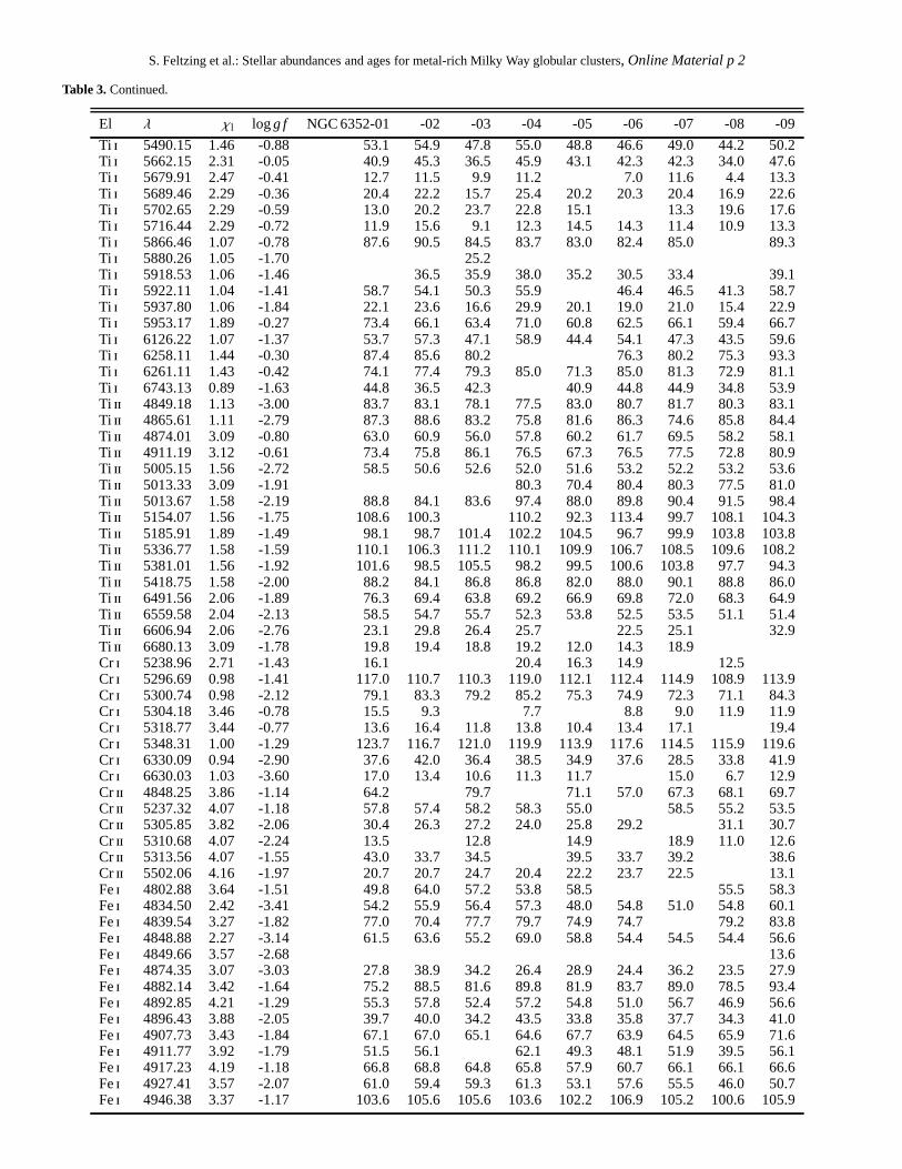
S. Feltzing et al.: Stellar abundances and ages for metal-rich Milky Way globular clusters, Online Material p 2
Table 3.Continued.
El λ χl logg f NGC 6352-01 -02 -03 -04 -05 -06 -07 -08 -09
Ti i 5490.15 1.46 -0.88 53.1 54.9 47.8 55.0 48.8 46.6 49.0 44.2 50.2Ti i 5662.15 2.31 -0.05 40.9 45.3 36.5 45.9 43.1 42.3 42.3 34.0 47.6Ti i 5679.91 2.47 -0.41 12.7 11.5 9.9 11.2 7.0 11.6 4.4 13.3Ti i 5689.46 2.29 -0.36 20.4 22.2 15.7 25.4 20.2 20.3 20.4 16.9 22.6Ti i 5702.65 2.29 -0.59 13.0 20.2 23.7 22.8 15.1 13.3 19.6 17.6Ti i 5716.44 2.29 -0.72 11.9 15.6 9.1 12.3 14.5 14.3 11.4 10.9 13.3Ti i 5866.46 1.07 -0.78 87.6 90.5 84.5 83.7 83.0 82.4 85.0 89.3Ti i 5880.26 1.05 -1.70 25.2Ti i 5918.53 1.06 -1.46 36.5 35.9 38.0 35.2 30.5 33.4 39.1Ti i 5922.11 1.04 -1.41 58.7 54.1 50.3 55.9 46.4 46.5 41.3 58.7Ti i 5937.80 1.06 -1.84 22.1 23.6 16.6 29.9 20.1 19.0 21.0 15.4 22.9Ti i 5953.17 1.89 -0.27 73.4 66.1 63.4 71.0 60.8 62.5 66.1 59.4 66.7Ti i 6126.22 1.07 -1.37 53.7 57.3 47.1 58.9 44.4 54.1 47.3 43.5 59.6Ti i 6258.11 1.44 -0.30 87.4 85.6 80.2 76.3 80.2 75.3 93.3Ti i 6261.11 1.43 -0.42 74.1 77.4 79.3 85.0 71.3 85.0 81.3 72.9 81.1Ti i 6743.13 0.89 -1.63 44.8 36.5 42.3 40.9 44.8 44.9 34.8 53.9Ti ii 4849.18 1.13 -3.00 83.7 83.1 78.1 77.5 83.0 80.7 81.7 80.3 83.1Ti ii 4865.61 1.11 -2.79 87.3 88.6 83.2 75.8 81.6 86.3 74.6 85.8 84.4Ti ii 4874.01 3.09 -0.80 63.0 60.9 56.0 57.8 60.2 61.7 69.5 58.2 58.1Ti ii 4911.19 3.12 -0.61 73.4 75.8 86.1 76.5 67.3 76.5 77.5 72.8 80.9Ti ii 5005.15 1.56 -2.72 58.5 50.6 52.6 52.0 51.6 53.2 52.2 53.2 53.6Ti ii 5013.33 3.09 -1.91 80.3 70.4 80.4 80.3 77.5 81.0Ti ii 5013.67 1.58 -2.19 88.8 84.1 83.6 97.4 88.0 89.8 90.4 91.5 98.4Ti ii 5154.07 1.56 -1.75 108.6 100.3 110.2 92.3 113.4 99.7 108.1 104.3Ti ii 5185.91 1.89 -1.49 98.1 98.7 101.4 102.2 104.5 96.7 99.9 103.8 103.8Ti ii 5336.77 1.58 -1.59 110.1 106.3 111.2 110.1 109.9 106.7 108.5109.6 108.2Ti ii 5381.01 1.56 -1.92 101.6 98.5 105.5 98.2 99.5 100.6 103.8 97.7 94.3Ti ii 5418.75 1.58 -2.00 88.2 84.1 86.8 86.8 82.0 88.0 90.1 88.8 86.0Ti ii 6491.56 2.06 -1.89 76.3 69.4 63.8 69.2 66.9 69.8 72.0 68.3 64.9Ti ii 6559.58 2.04 -2.13 58.5 54.7 55.7 52.3 53.8 52.5 53.5 51.1 51.4Ti ii 6606.94 2.06 -2.76 23.1 29.8 26.4 25.7 22.5 25.1 32.9Ti ii 6680.13 3.09 -1.78 19.8 19.4 18.8 19.2 12.0 14.3 18.9Cr i 5238.96 2.71 -1.43 16.1 20.4 16.3 14.9 12.5Cr i 5296.69 0.98 -1.41 117.0 110.7 110.3 119.0 112.1 112.4 114.9108.9 113.9Cr i 5300.74 0.98 -2.12 79.1 83.3 79.2 85.2 75.3 74.9 72.3 71.1 84.3Cr i 5304.18 3.46 -0.78 15.5 9.3 7.7 8.8 9.0 11.9 11.9Cr i 5318.77 3.44 -0.77 13.6 16.4 11.8 13.8 10.4 13.4 17.1 19.4Cr i 5348.31 1.00 -1.29 123.7 116.7 121.0 119.9 113.9 117.6 114.5115.9 119.6Cr i 6330.09 0.94 -2.90 37.6 42.0 36.4 38.5 34.9 37.6 28.5 33.8 41.9Cr i 6630.03 1.03 -3.60 17.0 13.4 10.6 11.3 11.7 15.0 6.7 12.9Cr ii 4848.25 3.86 -1.14 64.2 79.7 71.1 57.0 67.3 68.1 69.7Cr ii 5237.32 4.07 -1.18 57.8 57.4 58.2 58.3 55.0 58.5 55.2 53.5Cr ii 5305.85 3.82 -2.06 30.4 26.3 27.2 24.0 25.8 29.2 31.1 30.7Cr ii 5310.68 4.07 -2.24 13.5 12.8 14.9 18.9 11.0 12.6Cr ii 5313.56 4.07 -1.55 43.0 33.7 34.5 39.5 33.7 39.2 38.6Cr ii 5502.06 4.16 -1.97 20.7 20.7 24.7 20.4 22.2 23.7 22.5 13.1Fei 4802.88 3.64 -1.51 49.8 64.0 57.2 53.8 58.5 55.5 58.3Fei 4834.50 2.42 -3.41 54.2 55.9 56.4 57.3 48.0 54.8 51.0 54.8 60.1Fei 4839.54 3.27 -1.82 77.0 70.4 77.7 79.7 74.9 74.7 79.2 83.8Fei 4848.88 2.27 -3.14 61.5 63.6 55.2 69.0 58.8 54.4 54.5 54.4 56.6Fei 4849.66 3.57 -2.68 13.6Fei 4874.35 3.07 -3.03 27.8 38.9 34.2 26.4 28.9 24.4 36.2 23.5 27.9Fei 4882.14 3.42 -1.64 75.2 88.5 81.6 89.8 81.9 83.7 89.0 78.5 93.4Fei 4892.85 4.21 -1.29 55.3 57.8 52.4 57.2 54.8 51.0 56.7 46.9 56.6Fei 4896.43 3.88 -2.05 39.7 40.0 34.2 43.5 33.8 35.8 37.7 34.3 41.0Fei 4907.73 3.43 -1.84 67.1 67.0 65.1 64.6 67.7 63.9 64.5 65.9 71.6Fei 4911.77 3.92 -1.79 51.5 56.1 62.1 49.3 48.1 51.9 39.5 56.1Fei 4917.23 4.19 -1.18 66.8 68.8 64.8 65.8 57.9 60.7 66.1 66.1 66.6Fei 4927.41 3.57 -2.07 61.0 59.4 59.3 61.3 53.1 57.6 55.5 46.0 50.7Fei 4946.38 3.37 -1.17 103.6 105.6 105.6 103.6 102.2 106.9 105.2100.6 105.9

S. Feltzing et al.: Stellar abundances and ages for metal-rich Milky Way globular clusters, Online Material p 3
Table 3.Continued.
El λ χl logg f NGC 6352-01 -02 -03 -04 -05 -06 -07 -08 -09
Fei 4950.10 3.41 -1.67 82.4 87.5 80.1 87.0 81.7 74.2 83.6 85.1Fei 4961.92 3.63 -2.19 32.8 31.3 33.4 32.3 35.4 34.1 28.9 30.1 34.7Fei 4962.57 4.18 -1.18 57.7 51.9 54.1 55.3 52.3 52.9 52.9 49.6 54.4Fei 4969.91 4.21 -0.71 78.7 78.1 76.9 79.5 72.8 80.2 80.2 73.6 83.1Fei 4979.58 3.64 -2.58 24.2 28.7 21.2 26.3 19.6 22.3 19.9 20.8 24.2Fei 4985.25 3.92 -0.56 95.2 94.4 83.3 92.9 91.5 95.9 98.7 93.5 97.0Fei 4985.54 2.86 -1.33 116.6 119.2 111.7 115.0 105.6 111.9 111.2112.4 116.7Fei 4986.22 4.21 -1.39 49.1 49.2 52.1 55.6 43.3 48.3 47.5 40.6 50.2Fei 4999.11 4.18 -1.74 37.6 31.6 48.2 40.3 25.0 35.3 28.8 34.9Fei 5001.86 3.88 0.01 118.6 114.0 119.1 115.0 113.6 116.3 115.9 118.0 113.5Fei 5004.04 4.20 -1.40 47.8 45.2 48.6 57.8 44.0 44.4 48.7 45.5 51.7Fei 5012.69 4.28 -1.79 36.6 39.0 35.2 37.9 32.2 36.2 32.3 32.0 39.7Fei 5014.94 3.94 -0.30 114.5 110.9 112.2 118.2 116.2 111.3 111.5111.8 118.1Fei 5016.47 4.25 -1.69 18.7 31.4 32.4 36.3 34.2 32.7 26.0 31.5Fei 5028.12 3.57 -1.12 95.8 94.6 91.2 95.8 90.2 91.1 91.5 84.7 92.6Fei 5031.91 4.37 -1.67 28.9 26.2 27.9 35.4 21.1 19.3 21.1 20.3 27.1Fei 5044.21 2.85 -2.06 90.2 91.0 95.1 90.7 92.2 90.1 90.7 88.4 93.2Fei 5054.64 3.64 -1.92 40.5 42.5 35.5 45.5 37.0 38.4 43.3 32.8 40.6Fei 5056.84 4.26 -1.96 30.8 35.1 25.1 29.2 21.1 24.5 29.6 21.4 35.7Fei 5058.49 3.64 -2.83 13.9 16.5 13.3 13.5 8.1 13.6 8.7 6.3 12.0Fei 5067.16 4.22 -0.97 72.0 75.5 70.3 70.0 67.0 69.5 68.1 68.6 71.9Fei 5083.33 0.95 -2.96 146.9 152.7 141.0 147.2 146.8 144.9 142.1138.1Fei 5088.15 4.15 -1.68 36.0 35.0 25.1 35.5 32.5 32.9 32.5 29.0 37.6Fei 5090.77 4.26 -0.40 81.9 91.8 83.5 90.7 85.8 90.5 92.4 86.5 88.9Fei 5104.44 4.28 -1.59 37.1 39.2 35.7 36.3 37.9 36.4 34.2 35.1 42.3Fei 5109.66 4.30 -0.98 67.7 68.8 71.1 73.7 66.9 64.2 71.7 63.0Fei 5115.77 3.57 -2.74 28.3 30.7 14.6 26.9 18.4 22.3 26.2 16.3 25.3Fei 5127.37 0.91 -3.31 130.2 129.4 129.7 123.7 132.1 133.3 130.7129.6 136.9Fei 5127.67 0.05 -6.12 55.7 56.9 50.3 62.0 55.2 51.6 48.7 49.5 55.9Fei 5141.75 2.42 -2.24 103.5 104.2 101.6 103.9 105.5 101.9 102.299.1 106.9Fei 5143.72 2.19 -3.79 44.4 38.3 37.1 44.7 33.2 35.2 35.3 32.7 43.0Fei 5145.09 2.19 -2.88 79.3 75.5 69.9 69.2 69.9 71.7 71.7 70.0 76.4Fei 5159.05 4.28 -0.82 64.7 63.5 68.3 67.5 59.1 61.8 65.5 64.6 65.8Fei 5187.91 4.14 -1.37 63.8 57.4 58.0 55.5 55.9 55.5 57.0 55.2 54.5Fei 5197.93 4.30 -1.64 34.9 35.1 32.5 41.8 40.4 28.8 34.8 30.4 32.1Fei 5198.71 2.22 -2.14 123.9 125.5 119.1 118.4 120.6 113.6 120.1112.5 121.0Fei 5209.88 3.23 -3.26 37.4 23.7 27.0 17.8 15.8 14.0Fei 5217.38 3.21 -1.16 117.0 117.2 109.8 111.6 111.0 113.6 110.3108.8 111.4Fei 5223.18 3.63 -1.78 30.2 39.0 29.7 32.9 28.3 37.7 29.8 31.8Fei 5242.49 3.63 -0.97 92.3 91.7 92.3 93.4 90.1 93.6 90.2 85.6Fei 5249.10 4.47 -1.48 35.3 38.4 24.2 39.8 30.8 36.6 34.3 30.7 36.8Fei 5253.03 2.27 -3.84 30.5 26.7 27.9 32.2 27.9 27.8 32.7 23.9 30.1Fei 5262.88 3.25 -2.66 25.5 25.9 29.4 20.0 31.3 28.4 21.1 21.9Fei 5263.86 3.57 -2.14 71.4 66.7 66.1 67.2 49.5 52.7 54.7 66.2Fei 5267.26 4.37 -1.77 26.3 23.8 23.7 30.3 19.8 20.4 31.4 20.0 19.2Fei 5285.12 4.43 -1.64 33.4 26.8 23.5 21.9 23.6 21.1 20.1 25.0Fei 5288.53 3.68 -1.51 65.2 62.3 69.3 65.6 62.9 64.7 66.3 62.6 65.8Fei 5293.95 4.14 -1.87 32.3 28.4 26.1 26.1 28.7 26.1 27.5 25.1 28.0Fei 5294.54 3.64 -2.76 15.6 16.5 10.5 16.0 18.1 13.9 12.1 12.4 11.6Fei 5295.31 4.41 -1.59 28.3 28.2 23.4 25.8 23.4 26.5 19.9 21.3 23.9Fei 5307.36 1.61 -2.99 121.1 119.3 111.6 123.7 119.7 117.8 117.6112.9 122.6Fei 5321.10 4.43 -0.95 39.2 41.3 38.8 39.7 37.8 39.5 39.0 38.9 41.7Fei 5322.04 2.28 -2.80 84.0 83.5 81.0 80.7 81.1 77.9 78.7 76.4 82.8Fei 5364.87 4.44 0.23 107.2 110.8 108.2 106.3 107.5 109.1 111.7 108.2 109.9Fei 5365.39 3.57 -1.02 86.0 92.4 87.6 82.4 91.2 83.3 87.9 84.5 85.3Fei 5367.46 4.41 0.44 113.1 121.8 115.6 114.3 119.4 109.0 116.5 112.9 121.2Fei 5373.69 4.47 -0.76 62.2 59.0 60.5 59.8 59.3 56.1 63.0 57.3 58.9Fei 5379.57 3.69 -1.51 65.3 69.3 69.8 64.4 65.1 64.2 64.9 57.6 66.1Fei 5383.36 4.31 0.64 127.8 134.7 130.6 128.6 130.4 131.6 133.0 124.0 130.9Fei 5386.33 4.15 -1.67 34.5 35.8 25.0 28.4 24.0 29.0 29.5 23.8 29.1
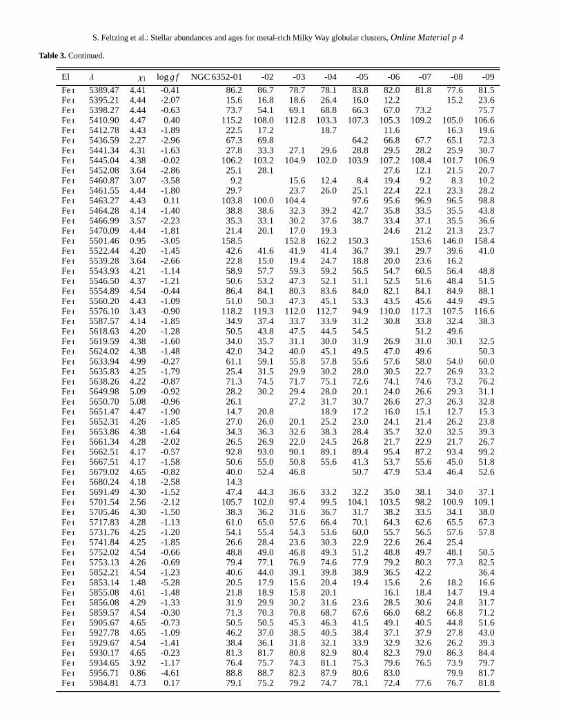
S. Feltzing et al.: Stellar abundances and ages for metal-rich Milky Way globular clusters, Online Material p 4
Table 3.Continued.
El λ χl logg f NGC 6352-01 -02 -03 -04 -05 -06 -07 -08 -09
Fei 5389.47 4.41 -0.41 86.2 86.7 78.7 78.1 83.8 82.0 81.8 77.6 81.5Fei 5395.21 4.44 -2.07 15.6 16.8 18.6 26.4 16.0 12.2 15.2 23.6Fei 5398.27 4.44 -0.63 73.7 54.1 69.1 68.8 66.3 67.0 73.2 75.7Fei 5410.90 4.47 0.40 115.2 108.0 112.8 103.3 107.3 105.3 109.2 105.0 106.6Fei 5412.78 4.43 -1.89 22.5 17.2 18.7 11.6 16.3 19.6Fei 5436.59 2.27 -2.96 67.3 69.8 64.2 66.8 67.7 65.1 72.3Fei 5441.34 4.31 -1.63 27.8 33.3 27.1 29.6 28.8 29.5 28.2 25.9 30.7Fei 5445.04 4.38 -0.02 106.2 103.2 104.9 102.0 103.9 107.2 108.4101.7 106.9Fei 5452.08 3.64 -2.86 25.1 28.1 27.6 12.1 21.5 20.7Fei 5460.87 3.07 -3.58 9.2 15.6 12.4 8.4 19.4 9.2 8.3 10.2Fei 5461.55 4.44 -1.80 29.7 23.7 26.0 25.1 22.4 22.1 23.3 28.2Fei 5463.27 4.43 0.11 103.8 100.0 104.4 97.6 95.6 96.9 96.5 98.8Fei 5464.28 4.14 -1.40 38.8 38.6 32.3 39.2 42.7 35.8 33.5 35.5 43.8Fei 5466.99 3.57 -2.23 35.3 33.1 30.2 37.6 38.7 33.4 37.1 35.5 36.6Fei 5470.09 4.44 -1.81 21.4 20.1 17.0 19.3 24.6 21.2 21.3 23.7Fei 5501.46 0.95 -3.05 158.5 152.8 162.2 150.3 153.6 146.0 158.4Fei 5522.44 4.20 -1.45 42.6 41.6 41.9 41.4 36.7 39.1 29.7 39.6 41.0Fei 5539.28 3.64 -2.66 22.8 15.0 19.4 24.7 18.8 20.0 23.6 16.2Fei 5543.93 4.21 -1.14 58.9 57.7 59.3 59.2 56.5 54.7 60.5 56.4 48.8Fei 5546.50 4.37 -1.21 50.6 53.2 47.3 52.1 51.1 52.5 51.6 48.4 51.5Fei 5554.89 4.54 -0.44 86.4 84.1 80.3 83.6 84.0 82.1 84.1 84.9 88.1Fei 5560.20 4.43 -1.09 51.0 50.3 47.3 45.1 53.3 43.5 45.6 44.9 49.5Fei 5576.10 3.43 -0.90 118.2 119.3 112.0 112.7 94.9 110.0 117.3 107.5 116.6Fei 5587.57 4.14 -1.85 34.9 37.4 33.7 33.9 31.2 30.8 33.8 32.4 38.3Fei 5618.63 4.20 -1.28 50.5 43.8 47.5 44.5 54.5 51.2 49.6Fei 5619.59 4.38 -1.60 34.0 35.7 31.1 30.0 31.9 26.9 31.0 30.1 32.5Fei 5624.02 4.38 -1.48 42.0 34.2 40.0 45.1 49.5 47.0 49.6 50.3Fei 5633.94 4.99 -0.27 61.1 59.1 55.8 57.8 55.6 57.6 58.0 54.0 60.0Fei 5635.83 4.25 -1.79 25.4 31.5 29.9 30.2 28.0 30.5 22.7 26.9 33.2Fei 5638.26 4.22 -0.87 71.3 74.5 71.7 75.1 72.6 74.1 74.6 73.2 76.2Fei 5649.98 5.09 -0.92 28.2 30.2 29.4 28.0 20.1 24.0 26.6 29.3 31.1Fei 5650.70 5.08 -0.96 26.1 27.2 31.7 30.7 26.6 27.3 26.3 32.8Fei 5651.47 4.47 -1.90 14.7 20.8 18.9 17.2 16.0 15.1 12.7 15.3Fei 5652.31 4.26 -1.85 27.0 26.0 20.1 25.2 23.0 24.1 21.4 26.2 23.8Fei 5653.86 4.38 -1.64 34.3 36.3 32.6 38.3 28.4 35.7 32.0 32.5 39.3Fei 5661.34 4.28 -2.02 26.5 26.9 22.0 24.5 26.8 21.7 22.9 21.7 26.7Fei 5662.51 4.17 -0.57 92.8 93.0 90.1 89.1 89.4 95.4 87.2 93.4 99.2Fei 5667.51 4.17 -1.58 50.6 55.0 50.8 55.6 41.3 53.7 55.6 45.0 51.8Fei 5679.02 4.65 -0.82 40.0 52.4 46.8 50.7 47.9 53.4 46.4 52.6Fei 5680.24 4.18 -2.58 14.3Fei 5691.49 4.30 -1.52 47.4 44.3 36.6 33.2 32.2 35.0 38.1 34.0 37.1Fei 5701.54 2.56 -2.12 105.7 102.0 97.4 99.5 104.1 103.5 98.2 100.9 109.1Fei 5705.46 4.30 -1.50 38.3 36.2 31.6 36.7 31.7 38.2 33.5 34.1 38.0Fei 5717.83 4.28 -1.13 61.0 65.0 57.6 66.4 70.1 64.3 62.6 65.5 67.3Fei 5731.76 4.25 -1.20 54.1 55.4 54.3 53.6 60.0 55.7 56.5 57.6 57.8Fei 5741.84 4.25 -1.85 26.6 28.4 23.6 30.3 22.9 22.6 26.4 25.4Fei 5752.02 4.54 -0.66 48.8 49.0 46.8 49.3 51.2 48.8 49.7 48.1 50.5Fei 5753.13 4.26 -0.69 79.4 77.1 76.9 74.6 77.9 79.2 80.3 77.3 82.5Fei 5852.21 4.54 -1.23 40.6 44.0 39.1 39.8 38.9 36.5 42.2 36.4Fei 5853.14 1.48 -5.28 20.5 17.9 15.6 20.4 19.4 15.6 2.6 18.2 16.6Fei 5855.08 4.61 -1.48 21.8 18.9 15.8 20.1 16.1 18.4 14.7 19.4Fei 5856.08 4.29 -1.33 31.9 29.9 30.2 31.6 23.6 28.5 30.6 24.8 31.7Fei 5859.57 4.54 -0.30 71.3 70.3 70.8 68.7 67.6 66.0 68.2 66.8 71.2Fei 5905.67 4.65 -0.73 50.5 50.5 45.3 46.3 41.5 49.1 40.5 44.8 51.6Fei 5927.78 4.65 -1.09 46.2 37.0 38.5 40.5 38.4 37.1 37.9 27.8 43.0Fei 5929.67 4.54 -1.41 38.4 36.1 31.8 32.1 33.9 32.9 32.6 26.2 39.3Fei 5930.17 4.65 -0.23 81.3 81.7 80.8 82.9 80.4 82.3 79.0 86.3 84.4Fei 5934.65 3.92 -1.17 76.4 75.7 74.3 81.1 75.3 79.6 76.5 73.9 79.7Fei 5956.71 0.86 -4.61 88.8 88.7 82.3 87.9 80.6 83.0 79.9 81.7Fei 5984.81 4.73 0.17 79.1 75.2 79.2 74.7 78.1 72.4 77.6 76.7 81.8

S. Feltzing et al.: Stellar abundances and ages for metal-rich Milky Way globular clusters, Online Material p 5
Table 3.Continued.
El λ χl logg f NGC 6352-01 -02 -03 -04 -05 -06 -07 -08 -09
Fei 6003.01 3.88 -1.12 80.8 87.0 81.7 83.5 82.3 84.6 82.3 82.4 86.7Fei 6012.20 2.22 -4.20 36.4 37.0 28.8 30.2 29.5 34.6 36.2 29.7 31.9Fei 6024.05 4.54 -0.12 95.6 93.7 101.2 97.6 91.4 93.5 99.4 94.4 97.5Fei 6027.05 4.07 -1.09 66.6 68.3 63.5 62.7 65.4 62.0 69.4 61.1 68.2Fei 6056.00 4.73 -0.46 65.7 64.9 61.5 61.7 58.4 60.4 61.4 62.4 65.7Fei 6065.48 2.61 -1.53 136.8 135.7 135.2 131.2 141.6 128.3 125.9124.8 147.1Fei 6079.00 4.65 -1.12 33.2 41.9 36.1 39.0 30.0 33.7 42.3 40.7 38.9Fei 6082.72 2.22 -3.57 55.3 49.5 50.9 51.5 47.3 51.6 50.8 54.0Fei 6085.26 2.75 -2.71 66.4 70.8 64.4 69.2 61.7 65.2 64.7 55.0 69.6Fei 6093.64 4.60 -1.40 21.8 27.9 24.3 24.5 23.6 22.2 27.0 21.8 28.1Fei 6094.37 4.65 -1.84 16.6 17.3 14.5 14.9 12.2 16.9 16.3 29.0 21.5Fei 6096.66 3.98 -1.83 37.8 37.6 33.8 38.2 40.1 36.2 26.3 36.6Fei 6120.24 0.91 -5.95 9.8 15.6 9.5 14.4 11.1 8.6 7.9 17.9Fei 6127.90 4.14 -1.40 50.4 52.6 46.5 49.1 47.9 52.5 47.6 45.2 55.6Fei 6137.69 2.58 -1.40 149.9 154.0 159.8 150.4 152.4 149.3 149.5141.8Fei 6151.61 2.17 -3.27 70.1 70.5 70.4 68.0 63.8 70.8 68.3 64.0 71.1Fei 6157.72 4.07 -1.16 70.7 66.8 67.0 59.3 65.6 66.3 67.5 62.5 68.7Fei 6159.37 4.60 -1.97 12.7 15.8 11.2 15.3 8.2 6.7 14.7 9.4 10.3Fei 6165.36 4.14 -1.47 44.0 45.1 44.4 45.2 38.3 43.4 46.6 41.3 46.3Fei 6173.34 2.22 -2.88 97.4 93.7 84.6 89.9 91.7 86.6 86.9 86.5 93.3Fei 6180.20 2.72 -2.59 77.0 71.4 68.9 73.0 71.4 72.2 70.5 66.9 76.5Fei 6187.99 3.94 -1.62 51.8 50.3 44.9 53.6 46.7 43.7 47.2 46.7 51.3Fei 6200.31 2.60 -2.44 94.2 87.4 85.3 83.0 88.2 85.6 88.0 82.2 89.6Fei 6213.43 2.22 -2.48 91.5 108.1 102.1 105.1 101.7 99.9 102.0 102.6 108.3Fei 6219.28 2.19 -2.42 118.5 116.7 101.1 112.0 110.3 115.1 111.7110.0 119.8Fei 6226.73 3.88 -2.12 26.7 26.8 22.2 25.2 23.6 27.7 25.4 19.2 29.2Fei 6229.22 2.84 -2.87 50.3 49.1 49.2 49.6 52.6 49.7 50.1 46.2 49.9Fei 6232.64 3.65 -0.96 90.5 87.0 86.3 85.6 87.7 84.7 89.4 82.2 89.8Fei 6246.31 3.60 -0.88 112.9 111.2 112.0 112.7 103.5 112.3 112.5106.6 118.8Fei 6252.55 2.40 -1.69 144.3 142.5 143.7 138.1 138.8 138.5 157.1134.0 152.4Fei 6265.14 2.18 -2.55 110.7 113.3 114.0 113.4 114.3 108.9 111.5115.5 114.9Fei 6270.22 2.85 -2.61 72.3 64.8 68.0 60.4 59.6 62.6 66.3 60.4 69.0Fei 6297.79 2.22 -2.73 99.5 102.9 96.1 100.3 97.1 97.4 105.5Fei 6302.49 3.68 -0.91 98.7 109.6 84.2 77.3 86.4 94.6 64.5Fei 6311.50 2.83 -3.23 40.3 47.1 38.3 40.2 44.3 38.9 40.1 37.0Fei 6322.68 2.58 -2.43 100.3 72.7 89.4 95.3 89.2 97.4 98.6 96.0 98.7Fei 6330.84 4.73 -1.74 33.6 24.3 24.4 22.8 22.8 23.8 25.3 24.0 25.8Fei 6335.33 2.19 -2.18 126.2 123.2 115.5 118.6 113.3 119.0 119.3116.9 122.4Fei 6336.82 3.68 -1.05 101.7 105.2 99.6 101.6 97.6 97.2 102.6 99.4 101.8Fei 6344.14 2.43 -2.92 83.9 79.6 72.6 76.7 72.9 73.6 79.7 70.5 81.0Fei 6355.02 2.84 -2.29 93.1 97.5 95.6 88.3 87.8 92.2Fei 6380.75 4.19 -1.38 57.6 55.1 52.2 51.8 51.6 56.2 57.4 75.6 60.1Fei 6392.53 2.27 -4.03 23.7 32.4 21.3 29.4 28.0 28.4 26.3 28.4 25.0Fei 6393.60 2.43 -1.58 148.0 147.2 152.6 143.0 156.9 140.4 140.0146.5 166.0Fei 6411.64 3.65 -0.72 121.3 120.7 115.3 112.7 116.3 117.6 120.9112.6 118.7Fei 6421.35 2.27 -2.03 144.1 141.5 137.3 135.6 141.5 141.1 139.3145.1Fei 6430.84 2.17 -2.01 145.4 142.2 138.0 139.9 139.7 135.0 138.9135.2 147.1Fei 6475.62 2.55 -2.94 75.0 77.3 72.0 76.1 72.2 71.8 73.1 68.6 75.4Fei 6481.87 2.27 -2.96 86.8 80.7 88.5 80.7 82.1 86.2 78.5 81.3 87.8Fei 6498.94 0.96 -4.70 95.4 90.4 86.1 95.1 87.4 91.7 82.7 75.2 100.4Fei 6533.92 4.55 -1.46 36.3 29.2 32.4 23.0 30.9 29.8 35.8Fei 6546.23 2.75 -1.54 127.7 127.8 124.0 115.4 118.6 118.0 120.0113.6 125.5Fei 6569.21 4.73 -0.42 72.9 73.4 77.2 76.1 69.6 60.6 70.1 74.7Fei 6574.22 0.99 -5.02 60.7 62.5 57.2 58.2 53.7 53.7 54.6 49.5 60.0Fei 6575.01 2.58 -2.71 86.0 81.7 85.5 84.7 85.0 83.2 81.9 82.0 86.6Fei 6592.91 2.73 -1.47 136.1 138.5 134.3 129.6 130.8 128.0 127.1134.5Fei 6593.87 2.43 -2.42 111.3 107.7 109.2 104.1 102.5 115.1 112.1106.9 109.3Fei 6597.56 4.79 -1.07 36.1 36.3 38.7 33.2 33.8 36.8 37.4 32.1 40.6Fei 6627.56 4.55 -1.58 18.2 23.2 28.1 26.9 25.2 19.7 25.2 23.8 20.7Fei 6646.93 2.60 -3.99 14.2 17.2 13.9 18.0 17.4 20.3 18.0 19.5 21.9
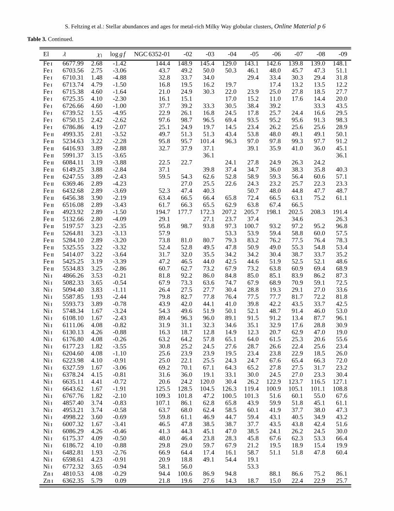
S. Feltzing et al.: Stellar abundances and ages for metal-rich Milky Way globular clusters, Online Material p 6
Table 3.Continued.
El λ χl logg f NGC 6352-01 -02 -03 -04 -05 -06 -07 -08 -09
Fei 6677.99 2.68 -1.42 144.4 148.9 145.4 129.0 143.1 142.6 139.8139.0 148.1Fei 6703.56 2.75 -3.06 43.7 49.2 50.0 50.3 46.1 48.0 45.7 47.3 51.1Fei 6710.31 1.48 -4.88 32.8 33.7 34.0 29.4 33.4 30.3 29.4 31.8Fei 6713.74 4.79 -1.50 16.8 19.5 16.2 19.7 17.4 13.2 13.5 12.2Fei 6715.38 4.60 -1.64 21.0 24.9 30.3 22.0 23.9 25.0 27.8 18.5 27.7Fei 6725.35 4.10 -2.30 16.1 15.1 17.0 15.2 11.0 17.6 14.4 20.0Fei 6726.66 4.60 -1.00 37.7 39.2 33.3 30.5 38.4 39.2 33.3 43.5Fei 6739.52 1.55 -4.95 22.9 26.1 16.8 24.5 17.8 25.7 24.4 16.6 29.5Fei 6750.15 2.42 -2.62 97.6 98.7 96.5 69.4 93.5 95.2 95.6 91.3 98.3Fei 6786.86 4.19 -2.07 25.1 24.9 19.7 14.5 23.4 26.2 25.6 25.6 28.9Feii 4993.35 2.81 -3.52 49.7 51.3 51.3 43.4 53.8 48.0 49.1 49.1 50.1Feii 5234.63 3.22 -2.28 95.8 95.7 101.4 96.3 97.0 97.8 99.3 97.7 91.2Feii 6416.93 3.89 -2.88 32.7 37.9 37.1 39.1 35.9 41.0 36.0 45.1Feii 5991.37 3.15 -3.65 36.1 36.1Feii 6084.11 3.19 -3.88 22.5 22.7 24.1 27.8 24.9 26.3 24.2Feii 6149.25 3.88 -2.84 37.1 39.8 37.4 34.7 36.0 38.3 35.8 40.3Feii 6247.55 3.89 -2.43 59.5 54.3 62.6 52.8 58.9 59.3 56.4 60.6 57.1Feii 6369.46 2.89 -4.23 27.0 25.5 22.6 24.3 23.2 25.7 22.3 23.3Feii 6432.68 2.89 -3.69 52.3 47.4 40.3 50.7 48.0 44.8 47.7 48.7Feii 6456.38 3.90 -2.19 63.4 66.5 66.4 65.8 72.4 66.5 63.1 75.2 61.1Feii 6516.08 2.89 -3.43 61.7 66.3 65.5 62.9 63.8 67.4 66.5Feii 4923.92 2.89 -1.50 194.7 177.7 172.3 207.2 205.7 198.1 202.5208.3 191.4Feii 5132.66 2.80 -4.09 29.1 27.1 23.7 37.4 34.6 26.3Feii 5197.57 3.23 -2.35 95.8 98.7 93.8 97.3 100.7 93.2 97.2 95.2 96.8Feii 5264.81 3.23 -3.13 57.9 53.3 53.9 59.4 58.8 60.0 57.5Feii 5284.10 2.89 -3.20 73.8 81.0 80.7 79.3 83.2 76.2 77.5 76.4 78.3Feii 5325.55 3.22 -3.32 52.4 52.8 49.5 47.8 50.9 49.0 55.3 54.8 53.4Feii 5414.07 3.22 -3.64 31.7 32.0 35.5 34.2 34.2 30.4 38.7 33.7 35.2Feii 5425.25 3.19 -3.39 47.2 46.5 44.0 42.5 44.6 51.9 52.5 52.1 48.6Feii 5534.83 3.25 -2.86 60.7 62.7 73.2 67.9 73.2 63.8 60.9 69.4 68.9Ni i 4866.26 3.53 -0.21 81.8 92.2 86.0 84.8 85.0 85.1 83.9 86.2 87.3Ni i 5082.33 3.65 -0.54 67.9 73.3 63.6 74.7 67.9 68.9 70.9 59.1 72.5Ni i 5094.40 3.83 -1.11 26.4 27.5 27.7 30.4 28.8 19.3 29.1 27.0 33.6Ni i 5587.85 1.93 -2.44 79.8 82.7 77.8 76.4 77.5 77.7 81.7 72.2 81.8Ni i 5593.73 3.89 -0.78 43.9 42.0 44.1 41.0 39.8 42.2 43.5 33.7 42.5Ni i 5748.34 1.67 -3.24 54.3 49.6 51.9 50.1 52.1 48.7 91.4 46.0 53.0Ni i 6108.10 1.67 -2.43 89.4 96.3 96.0 89.1 91.5 91.2 13.4 87.7 96.1Ni i 6111.06 4.08 -0.82 31.9 31.1 32.3 34.6 35.1 32.9 17.6 28.8 30.9Ni i 6130.13 4.26 -0.88 16.3 18.7 12.8 14.9 12.3 20.7 62.9 47.0 19.0Ni i 6176.80 4.08 -0.26 63.2 64.2 57.8 65.1 64.0 61.5 25.3 20.6 55.6Ni i 6177.23 1.82 -3.55 30.8 25.2 24.5 27.6 28.7 26.6 22.4 25.6 23.4Ni i 6204.60 4.08 -1.10 25.6 23.9 23.9 19.5 23.4 23.8 22.9 18.5 26.0Ni i 6223.98 4.10 -0.91 25.0 22.1 25.5 24.3 24.7 67.6 65.4 66.3 72.0Ni i 6327.59 1.67 -3.06 69.2 70.1 67.1 64.3 65.2 27.8 27.5 31.7 23.2Ni i 6378.24 4.15 -0.81 31.6 36.0 19.1 33.1 30.0 24.5 27.0 23.3 30.4Ni i 6635.11 4.41 -0.72 20.6 24.2 120.0 30.4 26.2 122.9 123.7 116.5 127.1Ni i 6643.62 1.67 -1.91 125.5 128.5 104.5 126.3 119.4 100.9 105.1101.1 108.8Ni i 6767.76 1.82 -2.10 109.3 101.8 47.2 100.5 101.3 51.6 60.1 55.0 67.6Ni i 4857.40 3.74 -0.83 107.1 86.1 62.8 65.8 43.9 59.9 51.8 45.1 61.1Ni i 4953.21 3.74 -0.58 63.7 68.0 62.4 58.5 60.1 41.9 37.7 38.0 47.3Ni i 4998.22 3.60 -0.69 59.8 61.1 46.9 44.7 59.4 43.1 40.5 34.9 43.2Ni i 6007.32 1.67 -3.41 46.5 47.8 38.5 38.7 37.7 43.5 43.8 42.4 51.6Ni i 6086.29 4.26 -0.46 41.3 44.3 45.1 47.0 38.5 24.1 26.2 24.5 30.0Ni i 6175.37 4.09 -0.50 48.0 46.4 23.8 28.3 45.8 67.6 62.3 53.3 66.4Ni i 6186.72 4.10 -0.88 29.8 29.0 59.7 67.9 21.2 19.5 18.9 15.4 19.9Ni i 6482.81 1.93 -2.76 66.9 64.4 17.4 16.1 58.7 51.1 51.8 47.8 60.4Ni i 6598.61 4.23 -0.91 20.9 18.8 49.1 54.4 19.1Ni i 6772.32 3.65 -0.94 58.1 56.0 53.3Zn i 4810.53 4.08 -0.29 94.4 100.6 86.9 94.8 88.1 86.6 75.2 86.1Zn i 6362.35 5.79 0.09 21.8 19.6 27.6 14.3 18.7 15.0 22.4 22.9 25.7


![, M. Kramer , J. Cordes arXiv:0811.0211v1 [astro-ph] 3 Nov ... · Lorimer & Kramer 2005) in the study of the Milky Way, globular clusters, the evolution and collapse of massive stars,](https://img.pdfslide.net/doc/110x75/5c6de26d09d3f2fe088c47d1/-m-kramer-j-cordes-arxiv08110211v1-astro-ph-3-nov-lorimer-kramer.jpg)