Embed Size (px)
Citation preview

Stellar Atmospheres: Radiative Equilibrium
1
Radiative Equilibrium
Energy conservation
Stellar Atmospheres: Radiative Equilibrium
2
Radiative Equilibrium
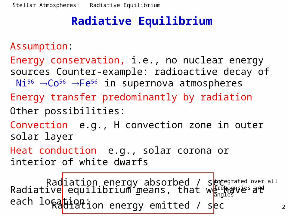
Assumption:
Energy conservation, i.e., no nuclear energy sources Counter-example: radioactive decay of Ni56 Co56 Fe56 in supernova atmospheres
Energy transfer predominantly by radiation
Other possibilities:
Convection e.g., H convection zone in outer solar layer
Heat conduction e.g., solar corona or interior of white dwarfs
Radiative equilibrium means, that we have at each location:
Radiation energy absorbed / sec =
Radiation energy emitted / sec
integrated over allfrequencies andangles

Stellar Atmospheres: Radiative Equilibrium
3
Radiative Equilibrium
Absorption per cm2 and second:
Emission per cm2 and second:
Assumption: isotropic opacities and emissivities
Integration over d then yields
Constraint equation in addition to the radiative transfer equation; fixes temperature stratification T(r)
4 0
)( vIvdvd
4 0
)(vdvd
0)( )()(000
dvSJvvdvJvdv vvv

Stellar Atmospheres: Radiative Equilibrium
4
Conservation of fluxAlternative formulation of energy equation
In plane-parallel geometry: 0-th moment of transfer equation
Integration over frequency, exchange integration and differentiation:
vvv SJ
dt
dH
0 0
4eff
0
4eff
0 0
0 because of radiative equilibrium
const for all depths. Alternatively written:4
(1st moment of transfer equat4
v v v
v
v
v
dH dv J S dv
dt
H H dv T
dv T dvdK
Hd
4eff
0
ion)
( ) (definiton of Eddington factor)
4
v vddv T
d
f J

Stellar Atmospheres: Radiative Equilibrium
5
Which formulation is good or better?
I Radiative equilibrium: local, integral form of energy equation
II Conservation of flux: non-local (gradient), differential form of radiative equilibrium
I / II numerically better behaviour in small / large depths
Very useful is a linear combination of both formulations:
A,B are coefficients, providing a smooth transition between formulations I and II.
0)(
00
Hdvd
JfdBdvSJA vv
vv
Stellar Atmospheres: Radiative Equilibrium
6
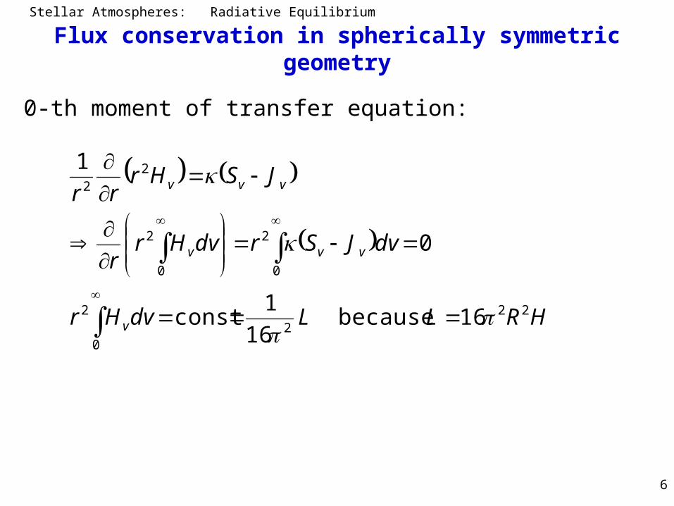
Flux conservation in spherically symmetric geometry
0-th moment of transfer equation:
HRLLdvHr
dvJSrdvHrr
JSHrrr
v
vvv
vvv
222
0
2
0
2
0
2
22
16 because 16
1const
0
1

Stellar Atmospheres: Radiative Equilibrium
7
Another alternative, if T de-couples from radiation field
Thermal balance of electrons
mllmlml
C
mllmlmm
H
kl
kThvv
lkvlkk
C
kl
lkvlkl
H
j
kThvvjj
C
jvjj
H
CH
hvTqnnQ
hvTqnnQ
dvec
hvJ
v
vJvnQ
dvv
vJvnQ
dvec
hvJTvNnQ
dvJTvNnQ
,ec
,ec
, 02
3
bf,bf
, 0
bf,bf
02
3
ff,eff
0
ff,eff
)(
)(
21)( 4
1)( 4
2
),( 4
),( 4
0

Stellar Atmospheres: Radiative Equilibrium
8
The gray atmosphereSimple but insightful problem to solve the transfer equation together with the constraint equation for radiative equilibrium
Gray atmosphere:
Moments of transfer equation
with
Integration over frequency
Radiative equilibrium ( ) ( ) 0
and because
v vv v v
v v v v
dH dKI J S II H dt
d d
dH dKI
J
J S II Hd d
J S dv J S dv J
S
S
I
1 2 1 2
2
2
of conservation of flux 0
from follows , see below0
dH
d
dKII K c c II c H
d
dc
K
d
Stellar Atmospheres: Radiative Equilibrium
9
The gray atmosphere
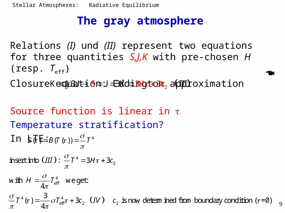
Relations (I) und (II) represent two equations for three quantities S,J,K with pre-chosen H (resp. Teff)
Closure equation: Eddington approximation
Source function is linear in Temperature stratification?
In LTE:
2K 1 3J J 3K IIIS 3H 3c
4
42
4eff
4 4eff 2 2
( ) ( ( ))
insert into : 3 3
with we get: 43
( ) 3 is now determined from boundary condition ( =0)4
S B T T
III T H c
H T
T T c IV c

Stellar Atmospheres: Radiative Equilibrium
10
Gray atmosphere: Outer boundary condition
Emergent flux:
3
23 ,
3
2
4
3
3
2
2
1
3
1
2
3)0(
)(12
1)( and
!)(with
)()( 2
3
)(332
1
from with )()(2
1)0(
4eff
4
22
12
0
0
22
0
2
0
22
0
2
HSTT
HccHH
ttEetEnl
ldttEt
dEcdEH
dEcH
IIISdESH
tn
l
from (IV): (from III)

Stellar Atmospheres: Radiative Equilibrium
11
Avoiding Eddington approximation
Ansatz:
Insert into Schwarzschild equation:
Approximate solution for J by iteration (“Lambda iteration“)
))((4
3)(
function Hopf )(
oftion generaliza ))((3)(
4eff
qTJ
q
IIIqHJ
0
1)(2
1)(
Jfor equation integral )(
dEqq
JSJ
)(2
1)(
3
1
3
23)32(3
)32(3
32)1()2(
)1(
EEHHJJ
HJ
(*) integral equation for q, see below
i.e., start with Eddington approximation
(was result for linear S)
Stellar Atmospheres: Radiative Equilibrium
12
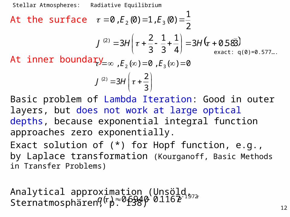
At the surface
At inner boundary
Basic problem of Lambda Iteration: Good in outer layers, but does not work at large optical depths, because exponential integral function approaches zero exponentially.
Exact solution of (*) for Hopf function, e.g., by Laplace transformation (Kourganoff, Basic Methods in Transfer Problems)
Analytical approximation (Unsöld, Sternatmosphären, p. 138)
358.034
1
3
1
3
23
2
1)0( , 1)0( , 0
)2(
32
HHJ
EE
2 3
(2)
, ( ) 0 , ( ) 0
23
3
E E
J H
972.11167.06940.0)( eq
exact: q(0)=0.577….

Stellar Atmospheres: Radiative Equilibrium
13
Gray atmosphere: Interpretation of resultsTemperature gradient
The higher the effective temperature, the steeper the temperature gradient.
The larger the opacity, the steeper the (geometric) temperature gradient.
Flux of gray atmosphere
d
dT
dt
dT
Td
dT
Td
dTTT
d
d
4eff
4eff
34
~
4
34
2 2
0
1/ 4
eff eff
LTE: ( ( ))
1 1( ) ( ( )) ( ) ( ( )) ( )
2 2
with , 3 4( ( )) ( ) ( )
and
v v
v v v
v
S B T
H B T E t dt B T E t dt
hv kT T T q p hv kT p
H d H dv H
3 3 3
2 3 3
4eff
43eff 2 2
4 3 2eff 0
1 2 4
2
4
( ) ( )4 4( ) /
exp( ( )) 1 exp( ( )) 1v
v
hv k k
hc h v
T
H kT E t E tdv kH H H dt dt
H d T h h c p p

Stellar Atmospheres: Radiative Equilibrium
14
Gray atmosphere: Interpretation of resultsLimb darkening of total radiation
i.e., intensity at limb of stellar disk smaller than at center by 40%, good agreement with solar observations
Empirical determination of temperature stratification
Observations at different wavelengths yield different T-structures, hence, the opacity must be a function of wavelength
4 4eff
3 2I( 0, ) S( ) B(T( )) T ( ) T
4 3
I(0, ) 2 / 3 2 3(1 cos )
I(0,1) 1 2 / 3 5 2
TTBSSI ))(()()( ),0( measure

Stellar Atmospheres: Radiative Equilibrium
15
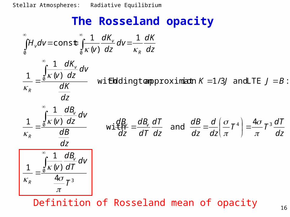
The Rosseland opacityGray approximation (=const) very coarse, ist there a good mean value ? What choice to make for a mean value?
For each of these 3 equations one can find a mean , with which the equations for the gray case are equal to the frequency-integrated non-gray equations. Because we demand flux conservation, the 1st moment equation is decisive for our choice: Rosseland mean of opacity
transfer equation
0-th moment
1st moment
non-gray gray
)( ISdz
dI ))(( vvv ISv
dz
dI
))(( vvv JSv
dz
dH
vv Hv
dz
dK)(
0)( JSdz
dH
Hdz
dK
Stellar Atmospheres: Radiative Equilibrium
16
The Rosseland opacity
Definition of Rosseland mean of opacity
3
0
340
0
00
4)(
1
1
4 and with
)(1
1
: LTE and 3/1ion approximatEddington with )(
1
1
1
)(
1const
T
dvdTdB
v
dz
dTTT
dz
d
dz
dB
dz
dT
dT
dB
dz
dB
dzdB
dvdzdB
v
BJJK
dzdK
dvdzdK
v
dz
dKdv
dz
dK
vdvH
v
R
vv
v
R
v
R
R
vv

Stellar Atmospheres: Radiative Equilibrium
17
The Rosseland opacity
The Rosseland mean is a weighted mean
of opacity with weight function
Particularly, strong weight is given to those frequencies, where the radiation flux is large. The corresponding optical depth is called Rosseland depth
For the gray approximation with is very good,
i.e.
R1
)(
1
v dT
dBv
R1Ross
z
RRoss zdzz0
)()(
))((4
3)( 4
eff4
RossRossRoss qTT
Stellar Atmospheres: Radiative Equilibrium
18
Convection
Compute model atmosphere assuming • Radiative equilibrium (Sect. VI) temperature stratification• Hydrostatic equilibrium pressure stratification
Is this structure stable against convection, i.e. small perturbations?
• Thought experiment
Displace a blob of gas by r upwards, fast enough that no heat exchange with surrounding occurs (i.e., adiabatic), but slow enough that pressure balance with surrounding is retained (i.e. << sound velocity)

Stellar Atmospheres: Radiative Equilibrium
19
Inside of blob outside
Stratification becomes unstable, if temperature gradient
rises above critical value.
( ), ( )T r r
ad ad
ad ad
( )
( )
T T T r r
r r
r
( ), ( )T r r
rad rad
rad rad
( )
( )
T T T r r
r r
ad rad
ad rad
ad rad
a
sta
( ) ( ) further buoyancy,
( ) ( ) gas blob falls back,
i.e.
with ideal gas equation p= and pressure balance
ble
stable
unstable
unsta
ble
H
r r r r
r r r r
d d
dr dr
kT
Am
d ad rad rad
ad radunstable
s
=
table
T T
dT dT
dr dr
addT dr
Stellar Atmospheres: Radiative Equilibrium
20
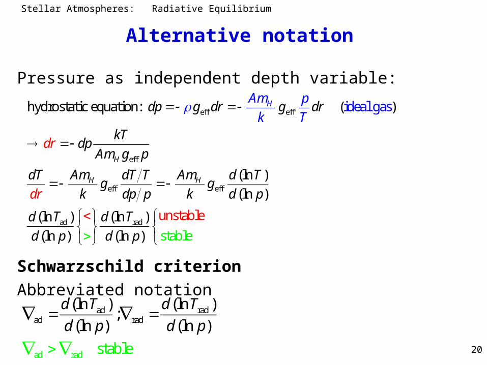
Alternative notation
Pressure as independent depth variable:
Schwarzschild criterion
Abbreviated notation
eff eff
eff
eff eff
ad rad
hydrostatic equation: ( )
(ln )
(ln )
(ln ) (ln )
(ln ) (
ide
unstabl
al gas
stabln
e
le )
H
H
H H
dp g dr g dr
kTdp
Am g p
Am AmdT dT T d Tg g
k dp p k d p
d T d T
d
d
Am p
k T
p d
r
dr
p
ad rada
ad d
d rad
ra
(ln ) (ln );
(ln ) (l
sta
n
b
)
le
d T d T
d p d p

Stellar Atmospheres: Radiative Equilibrium
21
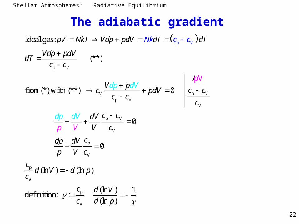
The adiabatic gradient
Internal energy of a one-atomic gas excluding effects of ionisation and excitation
But if energy can be absorbed by ionization:
Specific heat at constant pressure
V V
0 (no heat exchange)
(1st law of therm
intern 0 (al
ody
energy
namic
*)
s)
dQ
dQ pdV
c d
dE
dE c dT T pdV
V
3 3
2 2E NkT c Nk
V
3
2c Nk
p V Vt t
p V
( )
p cons p cons
c c
Q dE dV d NkT p Nkc p c p c p
T dT dT dT
Nk
p
Stellar Atmospheres: Radiative Equilibrium
22
The adiabatic gradient
p V
p VVp V
V
p
p V
V
V
p
V
p
V
Ideal gas:
(**)
/
from(*) with (**) 0
0
0
(ln ) (l
pV
n )
defi
pV NkT Vdp pdV dT dT
Vdp pdVdT
c c
V pc cc pdV
c cc
c cdV
p V c
cdp dV
dp d
p V c
cd V d p
V
d
Nk c
p d
V
c
c
V
p
V
(ln ) 1nition: :
(ln ) c d V
c d p
Stellar Atmospheres: Radiative Equilibrium
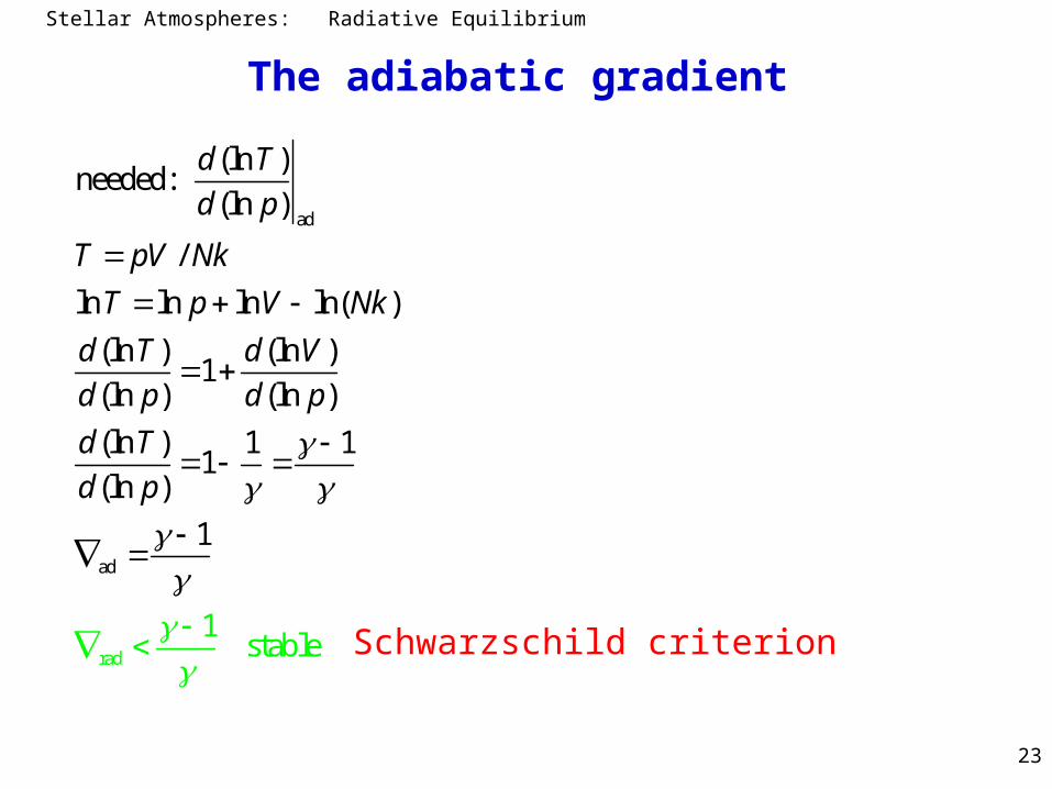
23
The adiabatic gradient
ad
ad
rad
(ln )needed:
(ln )
/
ln ln ln ln( )
(ln ) (ln )1
(ln ) (ln )
(ln ) 1 1
1 st
1(ln )
b e
1
a l
d T
d p
T pV Nk
T p V Nk
d T d V
d p d p
d T
d p
Schwarzschild criterion

Stellar Atmospheres: Radiative Equilibrium
24
The adiabatic gradient
• 1-atomic gas
• with ionization• Most important example: Hydrogen (Unsöld p.228)
V p V
ad
3 2 5 2
5 3 2 5 0.4
c Nk c c Nk Nk
ad1 0 convection starts effect
2Ion
ad 22Ion
2
2 5 2
5 5 2
( ) ( ) ( )with ionization degree
2 2
x x E kT
x x E kT
f T f T f Tx
N N N
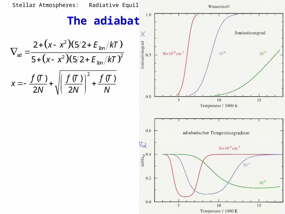
Stellar Atmospheres: Radiative Equilibrium
25
The adiabatic gradient
2Ion
ad 22Ion
2
2 5 2
5 5 2
( ) ( ) ( )
2 2
x x E kT
x x E kT
f T f T f Tx
N N N

Stellar Atmospheres: Radiative Equilibrium
26
Example: Grey approximation
4 4eff
4eff
1
3 2( ) 4 3
3 24ln ln ln4 3
2ln 34
hydrostatic equation: Ansatz: ( here a mass absorption coefficient)
(ln ) 124 3
1 integrate
1
b
b bb
T T
T T
d
d
dp gAp
dg g g
p pA b A
d T
Ap
dp
d
d
1
1
rad
rad
1
( 1)
1 1
( 1)24 3
becomes large, if opacity strongly increases with depth (i.e
(ln ) 1
(
. exponent b large).
The absolute value of is
1)
l
not
l
essenti
n
n
b b
b
g g
p p
d T
A
d
d p
d b
d p
p
p
d p
d
d
A
b
rad ad
a
l but
large
the change o
(> ): c
f with depth (g
onvection starts,
radient
-Ef ekt
)
f
Stellar Atmospheres: Radiative Equilibrium
27
Hydrogen convection zone in the Sun
-effect and -effect act together
Going from the surface into the interior: At T~6000K ionization of hydrogen begins
ad decreases and increases, because a) more and more
electrons are available to form H and b) the excitation of H is responsible for increased bound-free opacity
In the Sun: outer layers of atmosphere radiative
inner layers of atmosphere convective
In F stars: large parts of atmosphere convective
In O,B stars: Hydrogen completely ionized, atmosphere radiative; He I and He II ionization zones, but energy transport by convection inefficient
Video
Stellar Atmospheres: Radiative Equilibrium
28
Transport of energy by convectionConsistent hydrodynamical simulations very costly;
Ad hoc theory: mixing length theory (Vitense 1953)
Model: gas blobs rise and fall along distance l (mixing length). After moving by distance l they dissolve and the surrounding gas absorbs their energy.
Gas blobs move without friction, only accelerated by buoyancy;
detailed presentation in Mihalas‘ textbook (p. 187-190)
( ) = pressure scale height
mixing length parameter
=0.5 2
l H r H
Stellar Atmospheres: Radiative Equilibrium
29
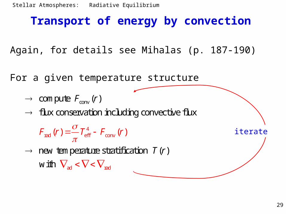
Transport of energy by convection
Again, for details see Mihalas (p. 187-190)
For a given temperature structure
4rad eff
conv
conv
ad rad
( )
compute ( )
flux conservation including convective flux
new temperature stratification ( )
wit
(
h
)
F r T F r
F r
T r
iterate

Stellar Atmospheres: Radiative Equilibrium
30
Summary: Radiative Equilibrium

Stellar Atmospheres: Radiative Equilibrium
31
Radiative Equilibrium:
Schwarzschildt Criterion:
Temperature of a gray Atmosphere
0)(
00
Hdvd
JfdBdvSJA vv
vv
4 4eff
3 2
4 3T T
ad rad(ln ) (ln )
(
unst
stable ln ) (
bl
ln
e
)
ad T d T
d p d p