Embed Size (px)
Citation preview
Step-by-step guide to creating webapps that display R script results on
Google dynamic maps with Rwui
Richard Newton and Lorenz Wernisch
July 7, 2012
1 Simple example
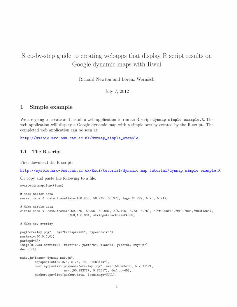
We are going to create and install a web application to run an R script dynmap_simple_example.R. Theweb application will display a Google dynamic map with a simple overlay created by the R script. Thecompleted web application can be seen at:
http://sysbio.mrc-bsu.cam.ac.uk/dynmap_simple_example.
1.1 The R script
First download the R script:
http://sysbio.mrc-bsu.cam.ac.uk/Rwui/tutorial/dynamic_map_tutorial/dynmap_simple_example.R
Or copy and paste the following to a file:
source(dynmap_functions)
# Make marker data
marker.data <- data.frame(lat=c(50.965, 50.975, 50.97), lng=c(5.722, 5.75, 5.74))
# Make circle data
circle.data <- data.frame(c(50.975, 50.96, 50.98), c(5.725, 5.73, 5.76), c("#0000FF","#FFD700","#DC143C"),
c(50,150,90), stringsAsFactors=FALSE)
# Make toy overlay
png("overlay.png", bg="transparent", type="cairo")
par(mai=c(0,0,0,0))
par(xpd=NA)
image(0,0,as.matrix(0), xaxt="n", yaxt="n", xlab=NA, ylab=NA, bty="n")
dev.off()
make.js(fname="dynmap_sub.js",
mapops=list(50.975, 5.74, 14, "TERRAIN"),
overlayops=list(pngname="overlay.png", sw=c(50.965783, 5.731112),
ne=c(50.992717, 5.76517), def.op=45),
markersops=list(marker.data, iconimage=NULL),
1
circlesops=list(circle.data),
clickable=FALSE)
1.2 Helper functions
You will also need to download the file dynmap_functions.R from:
http://sysbio.mrc-bsu.cam.ac.uk/Rwui/tutorial/dynamic_map_tutorial/dynmap_functions.R
1.3 Creating the webapp with Rwui
• Go to Rwui at: http://sysbio.mrc-bsu.cam.ac.uk/Rwui and click Start Rwui
• Enter a title for the application
Type Dynamic map simple example in the top box and click Enter
• Enter an introductory explanation (optional)
Leave blank and click Enter
• Include further instructions (optional)
Leave blank and click Enter
• Choose a variable input item
Ignore and click Finished composing page
• Validation
Leave as default and click Enter
• Enter a name for the application
Type dynmap_simple_example and click Enter
• Enter the name of a results file to be displayed (optional)
Type dynmap_sub.js
Tick the checkbox by ‘Tick box if file is a dynamic geographic map’
Click Enter
Click Finished entering filenames
• Enter the name of a list of results files (optional)
Ignore and click Finished entering filenames
• Layout of results files
Leave as default and click Enter
2
• Number of columns in the layout tables
Leave as default and click Enter
• Display results on the analysis page?
Tick check box by ‘Tick box to display results on the analysis page’ and click Enter
• Process information
Ignore and click Enter
• Graphical process information
Ignore and click Enter
• Upload R script
Browse to location where you have saved the downloaded R script dynmap_simple_example.R andclick Enter
• Upload subsidiary R scripts and data sources (optional)
In the top box type dynmap_functions
Browse to location where you have saved the downloaded file dynmap_functions.R and click Enter
Click Finished entering subsidiary files
• Add an initial Login page?
Leave as default and click Enter
• Which way to return results to user?
Leave as default and click Enter
• Include a Cancel button on the web page
Ignore and click Enter
• Create application
Click Create application
• Completed
Click dynmap_simple_example.tgz (or dynmap_simple_example.zip, unpacked they are identical)and save file to your PC
• You are now finished with Rwui.
1.4 Installing Java
• Download the Java SE Runtime Environment (JRE) from:
http://www.oracle.com/technetwork/java/javase/downloads/index.html
3
• Install the JRE on your PC according to the instructions included with the release, or linked to onthe above page.
• Set an environment variable named JRE_HOME to the pathname of the directory into which youinstalled the JRE:
On Windows if the path is e.g. c:\jre6.0, then
– Right click on the My Computer icon on your desktop and select properties
– Click the Advanced Tab
– Click the Environment Variables button
– Under System Variable, click New
– Enter the variable name as JRE HOME
– Enter the variable value as the install path for the JRE e.g. c:\jre6.0
– Click OK
– Click Apply Changes
Or on Linux if the path is e.g. /usr/local/java/jre6.0 then
– Add the line export JRE_HOME=/usr/local/java/jre6.0 to file .bash_profile
– Save
– Run source ~/.bash_profile
• You may also use the full JDK rather than just the JRE. In this case set the JAVA_HOME environmentvariable to the pathname of the directory into which you installed the JDK, e.g. c:\jdk6.0 or/usr/local/java/jdk6.0.
1.5 Installing Tomcat
• Download a binary distribution of Tomcat from:
http://tomcat.apache.org
• Unpack the binary distribution into a convenient location on your PC.
• This will create a directory called eg. apache-tomcat-6.0.35.
• NB. On Windows - install into a directory called, for example, C:\tomcat\apache-tomcat-6-0-35.The path must not have any spaces, which prevent applications from running. Dots in the directorynames also cause problems, as might other characters, so just use alphanumerics and hyphens asshown in the example.
• From here on we will refer to the path to Tomcat (eg /usr/local/apache-tomcat-6.0.35 orc:\tomcat\apache-tomcat-6-0-35) as TOMCAT_HOME
4
• Tomcat can be started by executing the following commands:
\TOMCAT_HOME\bin\startup.bat (Windows)
/TOMCAT_HOME/bin/startup.sh (Linux)
• NB. On Linux make sure startup.sh is executable first
• Open a browser and type http://localhost:8080 in the address bar and this should take you toTomcat’s home page on your machine, indicating Tomcat is installed correctly and working.
1.6 Path to R
1.6.1 Linux
Nothing needs to be done on a Linux machine.
1.6.2 Windows
Need to set the path to R’s bin directory
• Right click on the My Computer icon on your desktop and select properties
• Click the Advanced Tab
• Click the Environment Variables button
• In the ‘System Variables’ box scroll down and select variable ‘Path’ and press ’Edit’
• Add the path to R’s bin directory by adding eg. C:\Program Files\R\R-2.12.0\bin to the ‘;’separated list
• Click OK
• Click Apply Changes
1.7 Installing the web application
• If you downloaded the tgz file unpack it: tar zxvf dynmap_simple_example.tgz
• Or if you downloaded the zip file unpack it: unzip dynmap_simple_example.zip
• A directory called dynmap_simple_example will have been created by the unpacking
• Copy the file dynmap_simple_example/deploy/dynmap_simple_example.war to the directory:
/TOMCAT_HOME/webapps
• Tomcat should unpack the .war file automatically, but if not simply stop and start Tomcat and the.war file should unpack.
(Tomcat can be stopped by executing the following command:
5
\TOMCAT_HOME\bin\shutdown (Windows)
/TOMCAT_HOME/bin/shutdown.sh (Unix) )
• This will give a directory /TOMCAT_HOME/webapps/dynmap_simple_example
1.8 ProjectedOverlay.js
• Download file ProjectedOverlay.js from:
http://code.google.com/p/geoxml3/source/browse/trunk/
• Copy file ProjectedOverlay.js to directory /TOMCAT_HOME/webapps/dynmap_simple_example/
• Windows users note: care should be taken that downloading doesn’t surreptitiously add an extraextension to the filename eg. ProjectedOverlay.js.txt will not work. If in doubt copy and pastethe code from the web page into a file called ProjectedOverlay.js.
1.9 Sorting out the API key
• Follow the instructions for obtaining an Google Maps API key at:
https://developers.google.com/maps/documentation/javascript/tutorial#api_key
• Then, in a text editor, open file /TOMCAT_HOME/webapps/dynmap_simple_example/EnterData.jsp
• Locate the line (approx. line 31) reading:
src="http://maps.googleapis.com/maps/api/js?key=YOUR_API_KEY&sensor=false&libraries=geometry"
• Replace YOUR_API_KEY with the api key you have just obtained from Google.
• (Note: if you don’t currently have an API key you can simply remove the characters key=YOUR_API_KEY&from the above line)
• Do the same for file /TOMCAT_HOME/webapps/dynmap_simple_example/Results.jsp
1.10 Using the web application
• Open a browser and type http://localhost:8080/dynmap_simple_example in the address bar.
• You should see your webapp, the same as http://sysbio.mrc-bsu.cam.ac.uk/dynmap_simple_example
• Click Analyse
• You should see the Google dynamic map with overlay as shown in Figure 1.
• The opacity of the png overlay can be varied by the controls below the map.
• The map can be zoomed and panned and the type changed to satellite etc using the usual Googlemap controls.
6
1.11 Technical note
Note that the R script uses png() to create the overlay. png() allows you to create png files withtransparent backgrounds which is just what you need for an overlay. png uses ‘cairo’, ‘Xlib’ or ‘quartz’to create the png so R does need to be compiled with support for at least one of these in order to createthe overlay successfully. And for type = "Xlib", png() may not be usable unless the X11 display isavailable to the owner of the R process. type = "cairo" requires cairo 1.2 or later.
If png() is not supported, as a temporary measure you could substitute the following code to create theoverlay:
bitmap(file="overlay.png")
par(mai=c(0,0,0,0))
par(xpd=NA)
image(0,0,as.matrix(0), xaxt="n", yaxt="n", xlab=NA, ylab=NA, bty="n")
dev2bitmap(file="overlay.png")
dev.off()
The background will not be transparent but since this simple overlay has no background areas, in thiscase it doesn’t matter. bitmap requires ‘ghostscript’ to be installed.
7
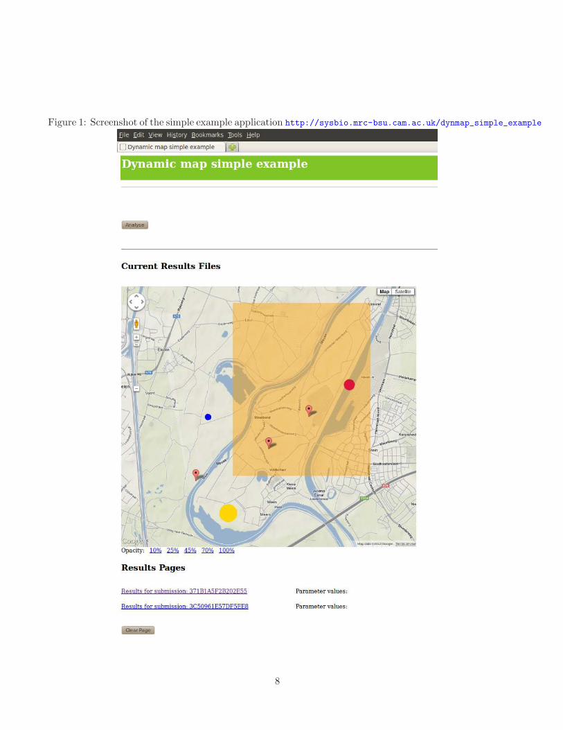
Figure 1: Screenshot of the simple example application http://sysbio.mrc-bsu.cam.ac.uk/dynmap_simple_example
8
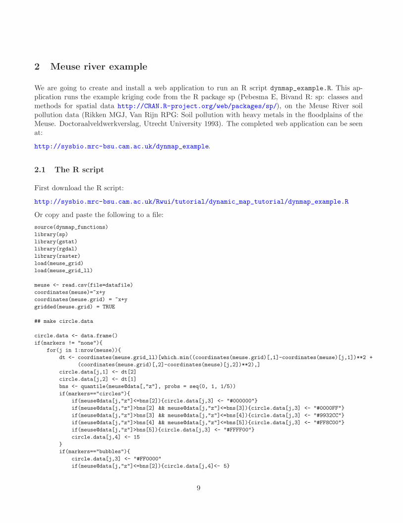
2 Meuse river example
We are going to create and install a web application to run an R script dynmap_example.R. This ap-plication runs the example kriging code from the R package sp (Pebesma E, Bivand R: sp: classes andmethods for spatial data http://CRAN.R-project.org/web/packages/sp/), on the Meuse River soilpollution data (Rikken MGJ, Van Rijn RPG: Soil pollution with heavy metals in the floodplains of theMeuse. Doctoraalveldwerkverslag, Utrecht University 1993). The completed web application can be seenat:
http://sysbio.mrc-bsu.cam.ac.uk/dynmap_example.
2.1 The R script
First download the R script:
http://sysbio.mrc-bsu.cam.ac.uk/Rwui/tutorial/dynamic_map_tutorial/dynmap_example.R
Or copy and paste the following to a file:
source(dynmap_functions)
library(sp)
library(gstat)
library(rgdal)
library(raster)
load(meuse_grid)
load(meuse_grid_ll)
meuse <- read.csv(file=datafile)
coordinates(meuse)=~x+y
coordinates(meuse.grid) = ~x+y
gridded(meuse.grid) = TRUE
## make circle.data
circle.data <- data.frame()
if(markers != "none"){
for(j in 1:nrow(meuse)){
dt <- coordinates(meuse.grid_ll)[which.min((coordinates(meuse.grid)[,1]-coordinates(meuse)[j,1])**2 +
(coordinates(meuse.grid)[,2]-coordinates(meuse)[j,2])**2),]
circle.data[j,1] <- dt[2]
circle.data[j,2] <- dt[1]
bns <- quantile(meuse@data[,"z"], probs = seq(0, 1, 1/5))
if(markers=="circles"){
if(meuse@data[j,"z"]<=bns[2]){circle.data[j,3] <- "#000000"}
if(meuse@data[j,"z"]>bns[2] && meuse@data[j,"z"]<=bns[3]){circle.data[j,3] <- "#0000FF"}
if(meuse@data[j,"z"]>bns[3] && meuse@data[j,"z"]<=bns[4]){circle.data[j,3] <- "#9932CC"}
if(meuse@data[j,"z"]>bns[4] && meuse@data[j,"z"]<=bns[5]){circle.data[j,3] <- "#FF8C00"}
if(meuse@data[j,"z"]>bns[5]){circle.data[j,3] <- "#FFFF00"}
circle.data[j,4] <- 15
}
if(markers=="bubbles"){
circle.data[j,3] <- "#FF0000"
if(meuse@data[j,"z"]<=bns[2]){circle.data[j,4]<- 5}
9
if(meuse@data[j,"z"]>bns[2] && meuse@data[j,"z"]<=bns[3]){circle.data[j,4] <- 10}
if(meuse@data[j,"z"]>bns[3] && meuse@data[j,"z"]<=bns[4]){circle.data[j,4] <- 20}
if(meuse@data[j,"z"]>bns[4] && meuse@data[j,"z"]<=bns[5]){circle.data[j,4] <- 30}
if(meuse@data[j,"z"]>bns[5]){circle.data[j,4] <- 40}
}
}
}else{
circle.data <- NULL
}
circlesops <- list(circle.data)
### Krige and make overlay
overlayops <- NULL
if(kri != "none"){
v.ok = variogram(log(z)~1, meuse)
ok.model = fit.variogram(v.ok, vgm(1, "Exp", 500, 1))
v.uk = variogram(log(z)~sqrt(dist), meuse)
uk.model = fit.variogram(v.uk, vgm(1, "Exp", 300, 1))
meuse[["ff"]] = factor(meuse[["ffreq"]])
meuse.grid[["ff"]] = factor(meuse.grid[["ffreq"]])
v.sk = variogram(log(z)~ff, meuse)
sk.model = fit.variogram(v.sk, vgm(1, "Exp", 300, 1))
if(kri=="ordinary"){
kg = krige(log(z)~1, meuse, meuse.grid, model = ok.model)
}
if(kri=="universal"){
kg = krige(log(z)~sqrt(dist), meuse, meuse.grid, model = uk.model)
}
if(kri=="stratified"){
kg = krige(log(z)~ff, meuse, meuse.grid, model = sk.model)
}
kg[["se"]] = sqrt(kg[["var1.var"]])
if(disp == "prediction"){
dat <- cbind(kg@coords, kg@data[,1])
}
if(disp == "se"){
dat <- cbind(kg@coords, kg@data[,3])
}
## Project the data from Rijksdriehoek (RDH) (Netherlands topographical) map coordinates to google map coordinates
r<-rasterFromXYZ(dat)
projection(r)<-paste("+init=epsg:28992","+towgs84=565.237,50.0087,465.658,-0.406857,0.350733,-1.87035,4.0812")
r.goog <- projectRaster(r, crs="+init=epsg:3857")
## Find the UTM lat/longs of the corners of the google maps coordinates raster
r.utm.ext <- projectExtent(r.goog, crs="+init=epsg:4326")
sw <- c(ymin(r.utm.ext), xmin(r.utm.ext))
ne <- c(ymax(r.utm.ext), xmax(r.utm.ext))
## Create overlay png
10
png("overlay.png", type="cairo", bg="transparent", width=5*ncol(r.goog), height=5*nrow(r.goog),res=72)
par(mai=c(0,0,0,0))
par(xpd=NA)
image(rotate.image(as.matrix(r.goog)), main="", bty="n", xaxt="n", yaxt="n", col=topo.colors(30))
dev.off()
overlayops <- list(pngname="overlay.png", sw=sw, ne=ne, def.op=45)
}
make.js("dynmap_sub.js", mapops=list(50.975, 5.74, 14, "TERRAIN"), overlayops=overlayops, circlesops=circlesops)
### Make title and legend
if(kri=="none"){
title <- chem
}else{
if(disp=="prediction"){
title <- paste(chem, " - ", kri, " kriging", " - ", "prediction", sep="")
}else{
title <- paste(chem, " - ", kri, " kriging", " - ", "standard errors", sep="")
}
}
if(markers == "circles"){
legend <- c(paste("<", bns[2], sep=" "),
paste(bns[2], "-", bns[3], sep=" "),
paste(bns[3], "-", bns[4], sep=" "),
paste(bns[4], "-", bns[5], sep=" "),
paste(">", bns[5], sep=" "))
cols <- c("#000000","#0000FF", "#9932CC", "#FF8C00", "#FFFF00")
}
if(markers == "bubbles"){
legend <- c(paste("<", bns[2], sep=" "),
paste(bns[2], "-", bns[3], sep=" "),
paste(bns[3], "-", bns[4], sep=" "),
paste(bns[4], "-", bns[5], sep=" "),
paste(">", bns[5], sep=" "))
pt.cex <- c(5/6,10/6,20/6,30/6,40/6)
cols <- c("#FF0000")
}
png("legend.png", type="cairo", width=750, height=750,res=72)
if(kri != "none"){
rng <- range(as.matrix(r.goog), na.rm=T)
lz <- seq(rng[1],rng[2], len=100)
legend.z <- NULL
for(i in 1:10){
legend.z <- rbind(legend.z, lz)
}
image.default(1:10, lz, legend.z, main = title, xlim=c(1,100), cex.main=2, cex.axis=2, xlab=NA, ylab=NA,
bty="n", xaxt="n", col=topo.colors(30))
}else{
plot(0,1, main=title, xlab=NA, ylab=NA, bty="n", xaxt="n", yaxt="n", type="n", cex.main=2)
}
if(markers == "circles"){
legend("center", legend=legend, pch=19, col=cols, title="Measurements", cex=2, y.intersp=1.5)
11
}
if(markers == "bubbles"){
legend("center", legend=legend, pch=19, pt.cex=pt.cex, col=cols, title="Measurements",
cex=2, y.intersp=1.5)
}
dev.off()
This web application also requires two .Rdata files, meuse_grid.Rdata and meuse_grid_ll.Rdata, whichyou will upload as subsidiary files when creating the application with Rwui. You can download the twofiles at:
http://sysbio.mrc-bsu.cam.ac.uk/Rwui/tutorial/dynamic_map_tutorial/meuse_grid.Rdata
http://sysbio.mrc-bsu.cam.ac.uk/Rwui/tutorial/dynamic_map_tutorial/meuse_grid_ll.Rdata
2.2 Helper functions
You will also need to download the file dynmap_functions.R from:
http://sysbio.mrc-bsu.cam.ac.uk/Rwui/tutorial/dynamic_map_tutorial/dynmap_functions.R
2.3 Creating the webapp with Rwui
• Go to Rwui at: http://sysbio.mrc-bsu.cam.ac.uk/Rwui and click Start Rwui
• Enter a title for the application
Type Dynamic map example in the top box and click Enter
• Enter an introductory explanation (optional)
Paste the following in the box:
This demonstration application runs the example kriging code from the
<A href=http://cran.r-project.org/web/packages/sp/index.html target="_blank">sp</A> package of
Edzer Pebesma, Roger Bivand and others, on the data of M G J Rikken and R P G Van Rijn
(Soil pollution with heavy metals in the floodplains of the Meuse, Utrecht University, 1993).
<P>
Here are some data files that can be downloaded for analysis by this webapp:
<P>
<ul>
<li>
<A href=http://sysbio.mrc-bsu.cam.ac.uk/Rwui/tutorial/dynamic_map_tutorial/meuse_zinc.csv>Zinc</A>
</li>
<li>
<A href=http://sysbio.mrc-bsu.cam.ac.uk/Rwui/tutorial/dynamic_map_tutorial/meuse_copper.csv>Copper</A>
</li>
<li>
<A href=http://sysbio.mrc-bsu.cam.ac.uk/Rwui/tutorial/dynamic_map_tutorial/meuse_cadmium.csv>Cadmium</A>
12
</li>
<li>
<A href=http://sysbio.mrc-bsu.cam.ac.uk/Rwui/tutorial/dynamic_map_tutorial/meuse_lead.csv>Lead</A>
</li>
</ul>
Click Enter
• Include further instructions (optional)
Leave blank and click Enter
• Choose a variable input item
– Select Section heading from the drop-down list and click Enter
Type Enter name of pollutant in the top box and click Enter
– Select Text box from the drop-down list and click Enter
Type chem in the top box and click Enter
– Select Section heading from the drop-down list and click Enter
Type Upload data file in the top box and click Enter
– Select File Upload Box from the drop-down list and click Enter
Type datafile in the top box and click Enter
– Select Section heading from the drop-down list and click Enter
Type Display measurement points in the top box and click Enter
– Select Drop-down List from the drop-down list and click Enter
Type markers in the top box and click Enter
Leave on default radio-button (Text) and click Enter
Type circles and click Enter
Type bubbles and click Enter
Type none and click Enter
Click Finished entering list entries
– Select Section heading from the drop-down list and click Enter
Type Display Kriging in the top box and click Enter
– Select Drop-down List from the drop-down list and click Enter
Type kri in the top box and click Enter
Leave on default radio-button (Text) and click Enter
Type none and click Enter
13
Type ordinary and click Enter
Type universal and click Enter
Type stratified and click Enter
Click Finished entering list entries
– Select Section heading from the drop-down list and click Enter
Type Display prediction or standard errors in the top box
Check the lowest radio-button to reduce the font size.
Click Enter
– Select Drop-down List from the drop-down list and click Enter
Type disp in the top box and click Enter
Leave on default radio-button (Text) and click Enter
Type prediction and click Enter
Type se and click Enter
Click Finished entering list entries
– Click Finished composing page
• Validation
Leave as default and click Enter
• Enter a name for the application
Type dynmap_example and click Enter
• Enter the name of a results file to be displayed (optional)
Type dynmap_sub.js in the top box
Tick the checkbox by ‘Tick box if file is a dynamic geographic map’
Change the ‘Width’ to 750
Click Enter
Type legend.png in the top box
DO NOT Tick the checkbox by ‘Tick box if file is a dynamic geographic map’
Change the ‘Width’ to 750
Click Enter
Click Finished entering filenames
14
• Enter the name of a list of results files (optional)
Ignore and click Finished entering filenames
• Layout of results files
Leave as default and click Enter
• Number of columns in the layout tables
Change ‘Number of columns’ to 2 and click Enter
• Display results on the analysis page?
Tick check box by ‘Tick box to display results on the analysis page’ and click Enter
• Process information
Ignore and click Enter
• Graphical process information
Ignore and click Enter
• Upload R script
Browse to location where you have saved the downloaded R script dynmap_example.R and clickEnter
• Upload subsidiary R scripts and data sources (optional)
In the top box type dynmap_functions
Browse to location where you have saved the downloaded file dynmap_functions.R and click Enter
In the top box type meuse_grid
Browse to location where you have saved the downloaded file meuse_grid.Rdata and click Enter
In the top box type meuse_grid_ll
Browse to location where you have saved the downloaded file meuse_grid_ll.Rdata and click Enter
Click Finished entering subsidiary files
• Add an initial Login page?
Leave as default and click Enter
• Which way to return results to user?
Leave as default and click Enter
• Include a Cancel button on the web page
Ignore and click Enter
• Create application
Click Create application
15
• Completed
Click dynmap_example.tgz (or dynmap_example.zip, unpacked they are identical) to save file toyour PC
• You are now finished with Rwui.
2.4 Installing Java
• Download the Java SE Runtime Environment (JRE) from:
http://www.oracle.com/technetwork/java/javase/downloads/index.html
• Install the JRE on your PC according to the instructions included with the release, or linked to onthe above page.
• Set an environment variable named JRE_HOME to the pathname of the directory into which youinstalled the JRE:
On Windows if the path is e.g. c:\jre6.0, then
– Right click on the My Computer icon on your desktop and select properties
– Click the Advanced Tab
– Click the Environment Variables button
– Under System Variable, click New
– Enter the variable name as JRE HOME
– Enter the variable value as the install path for the JRE e.g. c:\jre6.0
– Click OK
– Click Apply Changes
Or on Linux if the path is e.g. /usr/local/java/jre6.0 then
– Add the line export JRE_HOME=/usr/local/java/jre6.0 to file .bash_profile
– Save
– Run source ~/.bash_profile
• You may also use the full JDK rather than just the JRE. In this case set the JAVA_HOME environmentvariable to the pathname of the directory into which you installed the JDK, e.g. c:\jdk6.0 or/usr/local/java/jdk6.0.
2.5 Installing Tomcat
• Download a binary distribution of Tomcat from:
http://tomcat.apache.org
16
• Unpack the binary distribution into a convenient location on your PC.
• This will create a directory called eg. apache-tomcat-6.0.35.
• NB. On Windows - install into a directory called, for example, C:\tomcat\apache-tomcat-6-0-35.The path must not have any spaces, which prevent applications from running. Dots in the directorynames also cause problems, as might other characters, so just use alphanumerics and hyphens asshown in the example.
• From here on we will refer to the path to Tomcat (eg /usr/local/apache-tomcat-6.0.35 orc:\tomcat\apache-tomcat-6-0-35) as TOMCAT_HOME
• Tomcat can be started by executing the following commands:
\TOMCAT_HOME\bin\startup.bat (Windows)
/TOMCAT_HOME/bin/startup.sh (Linux)
• NB. On Linux make sure startup.sh is executable first
• Open a browser and type http://localhost:8080 in the address bar and this should take you toTomcat’s home page on your machine, indicating Tomcat is installed correctly and working.
2.6 Path to R
2.6.1 Linux
Nothing needs to be done on a Linux machine.
2.6.2 Windows
Need to set the path to R’s bin directory
• Right click on the My Computer icon on your desktop and select properties
• Click the Advanced Tab
• Click the Environment Variables button
• In the ‘System Variables’ box scroll down and select variable ‘Path’ and press ’Edit’
• Add the path to R’s bin directory by adding eg. C:\Program Files\R\R-2.12.0\bin to the ‘;’separated list
• Click OK
• Click Apply Changes
17
2.7 R package requirements
The R script requires the following packages to be available: sp, gstat, rgdal, raster.
R package rgdal requires two libraries installed:
• PROJ.4: Cartographic Projections Library http://trac.osgeo.org/proj/
• GDAL: Geospatial Data Abstraction Library http://www.gdal.org/
2.8 Installing the web application
• If you downloaded the tgz file unpack it: tar zxvf dynmap_example.tgz
• Or if you downloaded the zip file unpack it: unzip dynmap_example.zip
• A directory called dynmap_example will have been created by the unpacking
• Copy the file dynmap_example/deploy/dynmap_example.war to the directory:
/TOMCAT_HOME/webapps
• Tomcat should unpack the .war file automatically, but if not simply stop and start Tomcat and the.war file should unpack.
(Tomcat can be stopped by executing the following command:
\TOMCAT_HOME\bin\shutdown (Windows)
/TOMCAT_HOME/bin/shutdown.sh (Unix) )
• This will give a directory /TOMCAT_HOME/webapps/dynmap_example
2.9 ProjectedOverlay.js
• Download file ProjectedOverlay.js from:
http://code.google.com/p/geoxml3/source/browse/trunk/
• Copy file ProjectedOverlay.js to directory /TOMCAT_HOME/webapps/dynmap_example/
2.10 Sorting out the API key
• Follow the instructions for obtaining an Google Maps API key at:
https://developers.google.com/maps/documentation/javascript/tutorial#api_key
• Then, in a text editor, open file /TOMCAT_HOME/webapps/dynmap_example/EnterData.jsp
• Locate the line (approx. line 31) reading:
src="http://maps.googleapis.com/maps/api/js?key=YOUR_API_KEY&sensor=false&libraries=geometry"
18
• Replace YOUR_API_KEY with the api key you have just obtained from Google.
• (Note: if you don’t currently have an API key you can simply remove the characters key=YOUR_API_KEY&from the above line)
• Do the same for file /TOMCAT_HOME/webapps/dynmap_example/Results.jsp
2.11 Using the web application
• First download a data file to analyse, eg. the zinc data file from:
http://sysbio.mrc-bsu.cam.ac.uk/Rwui/tutorial/dynamic_map_tutorial/meuse_zinc.csv
• Open a browser and type http://localhost:8080/dynmap_example in the address bar.
• You should see your webapp, the same as http://sysbio.mrc-bsu.cam.ac.uk/dynmap_example
• Type zinc in the text box at the top
• In the File Upload box browse to location where you have saved the data file meuse_zinc.csv
• Select ordinary in the ‘Display Kriging’ drop-down list
• Click Analyse
• You should see the Google dynamic map with data points as color-coded circles and overlay ofkriging predictions as shown in Figure 2.
• The opacity of the kriging predictions overlay can be varied by the controls below the map.
• The map can be zoomed and panned and the type changed to satellite imagery etc using the usualGoogle dynamic map controls.
• You will notice a link at the bottom of the page Results for submission: ###########, where########## is a string of characters. Clicking on this link opens a results page for this submission.
• Change the ‘Display measurement points’ to bubbles, the ‘Display Kriging’ selection to universal,and the ‘Display prediction or standard errors’ drop-down list to se and click Analyse.
• The display on the Google map will change according to the new selections and a further link to aresults page will appear at the bottom of the page. The link to the first results page is still theretoo. In this way the results of previous submissions can still be accessed
2.12 Technical note
Note that the R script uses png() to create the overlay. png() allows you to create png files withtransparent backgrounds which is just what you need for an overlay. png uses ‘cairo’, ‘Xlib’ or ‘quartz’to create the png so R does need to be compiled with support for at least one of these in order to createthe overlay successfully. And for type = "Xlib", png() may not be usable unless the X11 display isavailable to the owner of the R process. type = "cairo" requires cairo 1.2 or later.
19
If png() is not supported as a temporary measure you could substitute the following code to create theoverlay:
bitmap(file="overlay.png")
par(mai=c(0,0,0,0))
par(xpd=NA)
image(rotate.image(as.matrix(r.goog)), main="", bty="n", xaxt="n", yaxt="n", col=topo.colors(30))
dev2bitmap(file="overlay.png")
dev.off()
although the background will not be transparent. bitmap requires ‘ghostscript’ to be installed.
20
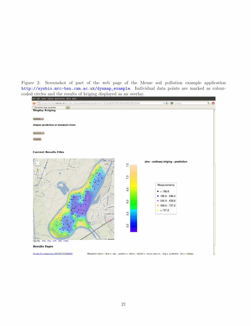
Figure 2: Screenshot of part of the web page of the Meuse soil pollution example applicationhttp://sysbio.mrc-bsu.cam.ac.uk/dynmap_example. Individual data points are marked as colour-coded circles and the results of kriging displayed as an overlay.
21