Embed Size (px)
Citation preview

Step by Step
Tutorial for AxisVM X4
Edited by: Inter-CAD Kft.
©2018 Inter-CAD Kft.
All rights reserved
All brand and product names are trademarks or registered trademarks.

Intentionally blank page

Step by step tutorial 3
TABLE OF CONTENTS
1. BEAM MODEL .................................................................................................................................................................................. 5
2. FRAME MODEL ............................................................................................................................................................................. 29
3. SLAB MODEL ................................................................................................................................................................................. 63
4. MEMBRANE MODEL .................................................................................................................................................................. 103
4.1. GEOMETRY DEFINITION USING PARAMETRIC MESH ..................................................................................................................... 103 4.2. GEOMETRY DEFINITION USING DOMAINS.................................................................................................................................... 112
5. SHELL MODEL ............................................................................................................................................................................ 127

4
Intentionally blank page

Step by step tutorial 5
1. BEAM MODEL
Objective The objective of this design example is to determine the internal forces, longitudinal reinforcement and
shear links of the two-span continuous reinforced concrete beam illustrated below. The loads will be
presented subsequently.
The cross-section is uniform along the beam: 400 mm*720 mm rectangle shape. The beam is analysed
according to Eurocode 2 standard.
Start
Start AxisVMX4 by double-clicking on AxisVMX4 icon in its installation folder, found in Start – Pro-
grams menu.
New
Create a new model by clicking on New icon. In the dialogue window replace Model file name with
‘beam’, select Eurocode from Design codes and set Unit and formats to EU.
If necessary, enter the name of Project and designer (Analysis by) at Page header. Company logo
also can be uploaded. This set page header will appear on the print image and documentation.
Click OK to close the dialog window.
Views
Check the view (workplane) of the model when starting a new model. On the left side of the main win-
dow find Views icon, open it with moving the cursor over the icon and select X-Z view. The actual view
is presented by the global coordinate system sign at the left bottom corner of the main window.
The global coordinate system can be changed during modelling, several local coordinate systems or
workplanes can be set. The directions of global coordinate system are marked with capital letters (X, Y
or Z). Please note that gravity force acts in -Z direction according to the default settings, but it can be
modified by the user.
Define of geometry - Elements
Select Elements tab to define geometry and structural properties of the beam. On the tab the icons of
available functions are displayed.
6
Draw objects
directly
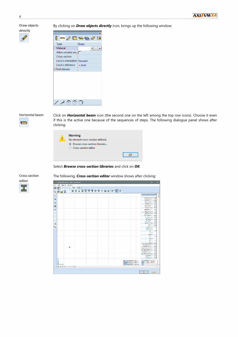
By clicking on Draw objects directly icon, brings up the following window:
Horizontal beam
Click on Horizontal beam icon (the second one on the left among the top row icons). Choose it even
if this is the active one because of the sequences of steps. The following dialogue panel shows after
clicking:
Select Browse cross-section libraries and click on OK.
Cross-section
editor
The following, Cross-section editor window shows after clicking:
Step by step tutorial 7
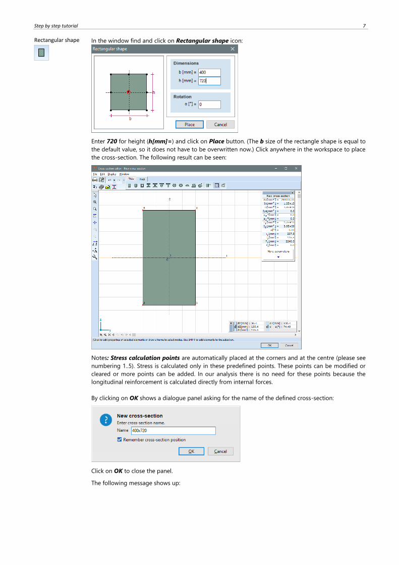
Rectangular shape
In the window find and click on Rectangular shape icon:
Enter 720 for height (h[mm]=) and click on Place button. (The b size of the rectangle shape is equal to
the default value, so it does not have to be overwritten now.) Click anywhere in the workspace to place
the cross-section. The following result can be seen:
Notes: Stress calculation points are automatically placed at the corners and at the centre (please see
numbering 1..5). Stress is calculated only in these predefined points. These points can be modified or
cleared or more points can be added. In our analysis there is no need for these points because the
longitudinal reinforcement is calculated directly from internal forces.
By clicking on OK shows a dialogue panel asking for the name of the defined cross-section:
Click on OK to close the panel.
The following message shows up:

8
By clicking on OK shows the following window:
Roll down in the list of Materials by using the vertical sliding bar (or simply roll down the mouse
wheel) and select C25/30, then click on OK to close the window.
Reference Leaving the references on auto option, the local x axis of the beam will be pointed in the direction of
the beam and the local z axis will be in the vertical plane.
The setup panel shows the following:
Step by step tutorial 9
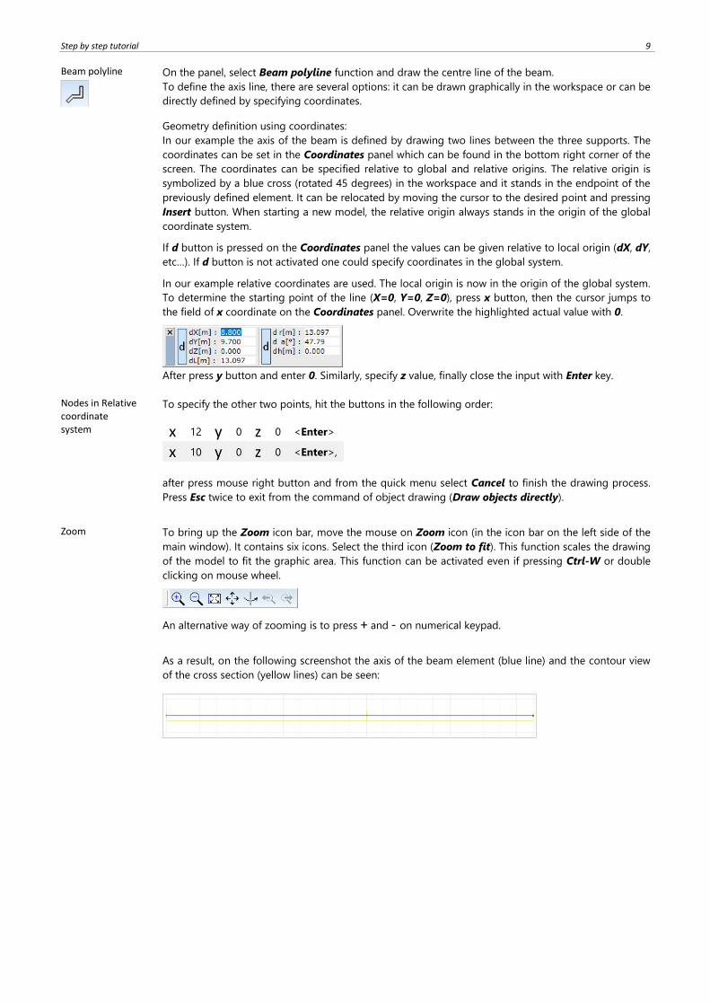
Beam polyline
On the panel, select Beam polyline function and draw the centre line of the beam.
To define the axis line, there are several options: it can be drawn graphically in the workspace or can be
directly defined by specifying coordinates.
Geometry definition using coordinates:
In our example the axis of the beam is defined by drawing two lines between the three supports. The
coordinates can be set in the Coordinates panel which can be found in the bottom right corner of the
screen. The coordinates can be specified relative to global and relative origins. The relative origin is
symbolized by a blue cross (rotated 45 degrees) in the workspace and it stands in the endpoint of the
previously defined element. It can be relocated by moving the cursor to the desired point and pressing
Insert button. When starting a new model, the relative origin always stands in the origin of the global
coordinate system.
If d button is pressed on the Coordinates panel the values can be given relative to local origin (dX, dY,
etc…). If d button is not activated one could specify coordinates in the global system.
In our example relative coordinates are used. The local origin is now in the origin of the global system.
To determine the starting point of the line (X=0, Y=0, Z=0), press x button, then the cursor jumps to
the field of x coordinate on the Coordinates panel. Overwrite the highlighted actual value with 0.
After press y button and enter 0. Similarly, specify z value, finally close the input with Enter key.
Nodes in Relative coordinate system
To specify the other two points, hit the buttons in the following order:
after press mouse right button and from the quick menu select Cancel to finish the drawing process.
Press Esc twice to exit from the command of object drawing (Draw objects directly).
x 12 y 0 z 0 <Enter>
x 10 y 0 z 0 <Enter>,
Zoom
To bring up the Zoom icon bar, move the mouse on Zoom icon (in the icon bar on the left side of the
main window). It contains six icons. Select the third icon (Zoom to fit). This function scales the drawing
of the model to fit the graphic area. This function can be activated even if pressing Ctrl-W or double
clicking on mouse wheel.
An alternative way of zooming is to press + and - on numerical keypad.
As a result, on the following screenshot the axis of the beam element (blue line) and the contour view
of the cross section (yellow lines) can be seen:
10
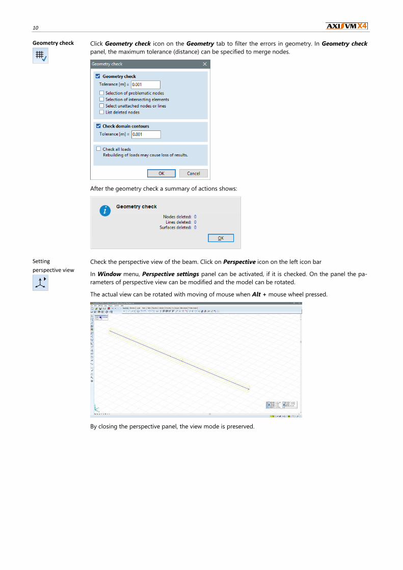
Geometry check
Click Geometry check icon on the Geometry tab to filter the errors in geometry. In Geometry check
panel, the maximum tolerance (distance) can be specified to merge nodes.
After the geometry check a summary of actions shows:
Setting
perspective view
Check the perspective view of the beam. Click on Perspective icon on the left icon bar
In Window menu, Perspective settings panel can be activated, if it is checked. On the panel the pa-
rameters of perspective view can be modified and the model can be rotated.
The actual view can be rotated with moving of mouse when Alt + mouse wheel pressed.
By closing the perspective panel, the view mode is preserved.
Step by step tutorial 11
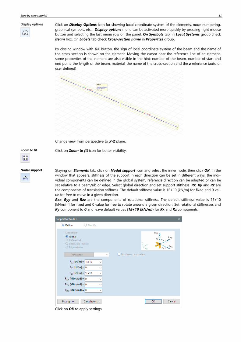
Display options
Click on Display Options icon for showing local coordinate system of the elements, node numbering,
graphical symbols, etc… Display options menu can be activated more quickly by pressing right mouse
button and selecting the last menu row on the panel. On Symbols tab, in Local Systems group check
Beam box. On Labels tab check Cross-section name in Properties group.
By closing window with OK button, the sign of local coordinate system of the beam and the name of
the cross-section is shown on the element. Moving the cursor near the reference line of an element,
some properties of the element are also visible in the hint: number of the beam, number of start and
end point, the length of the beam, material, the name of the cross-section and the z reference (auto or
user defined)
Change view from perspective to X-Z plane.
Zoom to fit
Click on Zoom to fit icon for better visibility.
Nodal support
Staying on Elements tab, click on Nodal support icon and select the inner node, then click OK. In the
window that appears, stiffness of the support in each direction can be set in different ways: the indi-
vidual components can be defined in the global system, reference direction can be adapted or can be
set relative to a beam/rib or edge. Select global direction and set support stiffness. Rx, Ry and Rz are
the components of translation stiffness. The default stiffness value is 1E+10 [kN/m] for fixed and 0 val-
ue for free to move in a given direction.
Rxx, Ryy and Rzz are the components of rotational stiffness. The default stiffness value is 1E+10
[kNm/m] for fixed and 0 value for free to rotate around a given direction. Set rotational stiffnesses and
Ry component to 0 and leave default values (1E+10 [kN/m]) for Rx and Rz components.
Click on OK to apply settings.
12
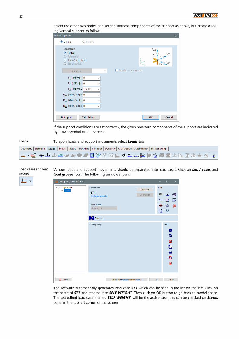
Select the other two nodes and set the stiffness components of the support as above, but create a roll-
ing vertical support as follow:
If the support conditions are set correctly, the given non-zero components of the support are indicated
by brown symbol on the screen.
Loads To apply loads and support movements select Loads tab.
Load cases and load groups
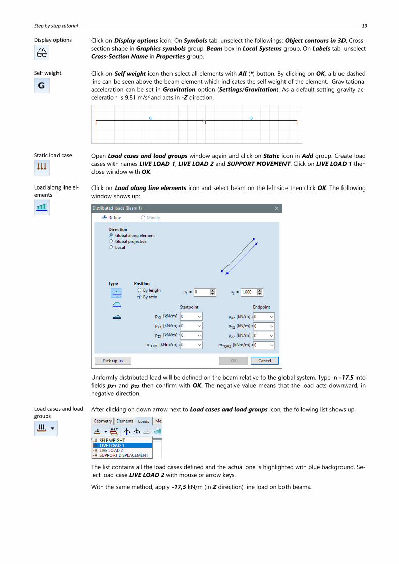
Various loads and support movements should be separated into load cases. Click on Load cases and
load groups icon. The following window shows:
The software automatically generates load case ST1 which can be seen in the list on the left. Click on
the name of ST1 and rename it to SELF WEIGHT. Then click on OK button to go back to model space.
The last edited load case (named SELF WEIGHT) will be the active case, this can be checked on Status
panel in the top left corner of the screen.
Step by step tutorial 13
Display options
Click on Display options icon. On Symbols tab, unselect the followings: Object contours in 3D, Cross-
section shape in Graphics symbols group, Beam box in Local Systems group. On Labels tab, unselect
Cross-Section Name in Properties group.
Self weight
Click on Self weight icon then select all elements with All (*) button. By clicking on OK, a blue dashed
line can be seen above the beam element which indicates the self weight of the element. Gravitational
acceleration can be set in Gravitation option (Settings/Gravitation). As a default setting gravity ac-
celeration is 9.81 m/s2 and acts in -Z direction.
Static load case
Open Load cases and load groups window again and click on Static icon in Add group. Create load
cases with names LIVE LOAD 1, LIVE LOAD 2 and SUPPORT MOVEMENT. Click on LIVE LOAD 1 then
close window with OK.
Load along line el-ements
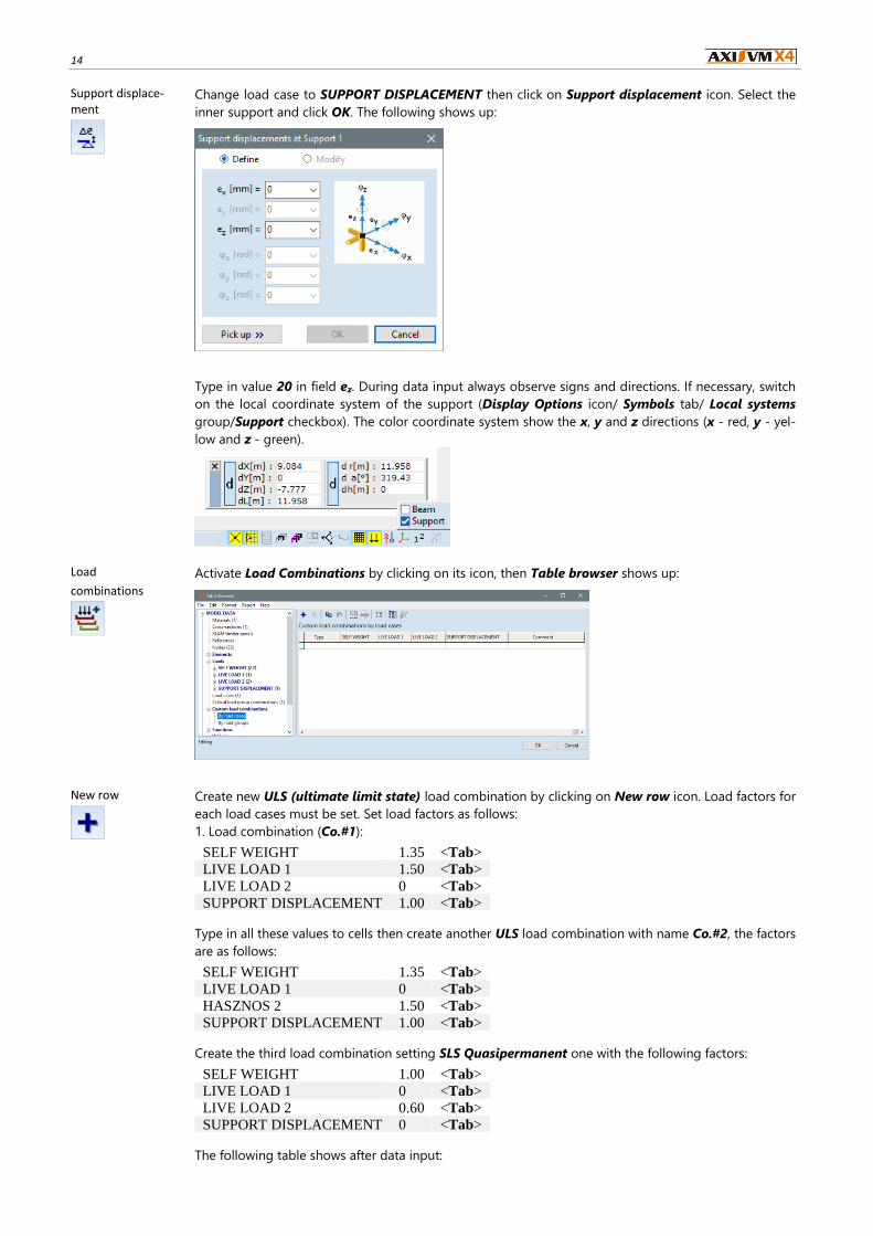
Click on Load along line elements icon and select beam on the left side then click OK. The following
window shows up:
Uniformly distributed load will be defined on the beam relative to the global system. Type in -17.5 into
fields pZ1 and pZ2 then confirm with OK. The negative value means that the load acts downward, in
negative direction.
Load cases and load groups
After clicking on down arrow next to Load cases and load groups icon, the following list shows up.
The list contains all the load cases defined and the actual one is highlighted with blue background. Se-
lect load case LIVE LOAD 2 with mouse or arrow keys.
With the same method, apply -17,5 kN/m (in Z direction) line load on both beams.
14
Support displace-ment
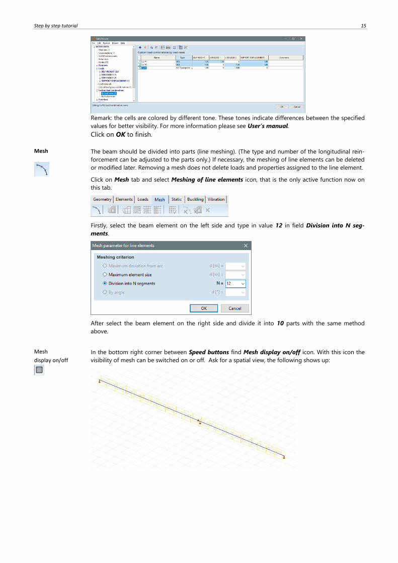
Change load case to SUPPORT DISPLACEMENT then click on Support displacement icon. Select the
inner support and click OK. The following shows up:
Type in value 20 in field ez. During data input always observe signs and directions. If necessary, switch
on the local coordinate system of the support (Display Options icon/ Symbols tab/ Local systems
group/Support checkbox). The color coordinate system show the x, y and z directions (x - red, y - yel-
low and z - green).
Load
combinations
Activate Load Combinations by clicking on its icon, then Table browser shows up:
New row
Create new ULS (ultimate limit state) load combination by clicking on New row icon. Load factors for
each load cases must be set. Set load factors as follows:
1. Load combination (Co.#1):
Type in all these values to cells then create another ULS load combination with name Co.#2, the factors
are as follows:
Create the third load combination setting SLS Quasipermanent one with the following factors:
The following table shows after data input:
SELF WEIGHT 1.35 <Tab>
LIVE LOAD 1 1.50 <Tab>
LIVE LOAD 2 0 <Tab>
SUPPORT DISPLACEMENT 1.00 <Tab>
SELF WEIGHT 1.35 <Tab>
LIVE LOAD 1 0 <Tab>
HASZNOS 2 1.50 <Tab>
SUPPORT DISPLACEMENT 1.00 <Tab>
SELF WEIGHT 1.00 <Tab>
LIVE LOAD 1 0 <Tab>
LIVE LOAD 2 0.60 <Tab>
SUPPORT DISPLACEMENT 0 <Tab>
Step by step tutorial 15
Remark: the cells are colored by different tone. These tones indicate differences between the specified
values for better visibility. For more information please see User’s manual.
Click on OK to finish.
Mesh
The beam should be divided into parts (line meshing). (The type and number of the longitudinal rein-
forcement can be adjusted to the parts only.) If necessary, the meshing of line elements can be deleted
or modified later. Removing a mesh does not delete loads and properties assigned to the line element.
Click on Mesh tab and select Meshing of line elements icon, that is the only active function now on
this tab.
Firstly, select the beam element on the left side and type in value 12 in field Division into N seg-
ments.
After select the beam element on the right side and divide it into 10 parts with the same method
above.
Mesh
display on/off
In the bottom right corner between Speed buttons find Mesh display on/off icon. With this icon the
visibility of mesh can be switched on or off. Ask for a spatial view, the following shows up:
16
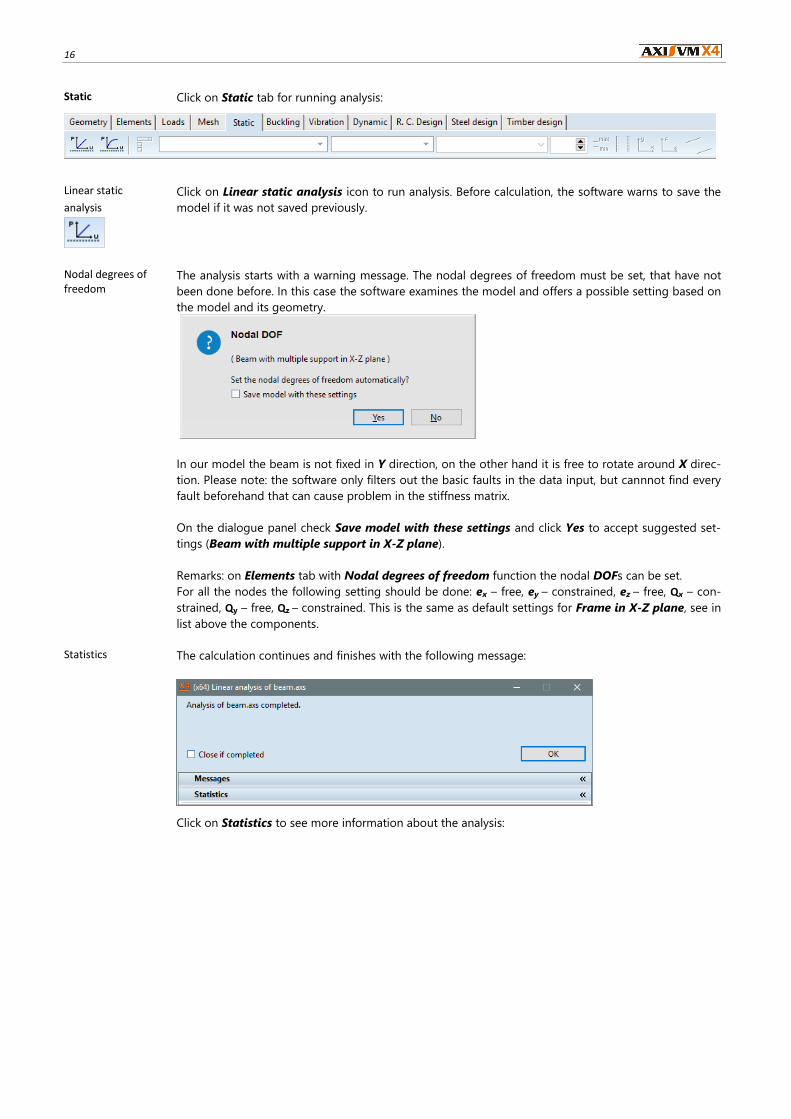
Static Click on Static tab for running analysis:
Linear static
analysis
Click on Linear static analysis icon to run analysis. Before calculation, the software warns to save the
model if it was not saved previously.
Nodal degrees of freedom
The analysis starts with a warning message. The nodal degrees of freedom must be set, that have not
been done before. In this case the software examines the model and offers a possible setting based on
the model and its geometry.
In our model the beam is not fixed in Y direction, on the other hand it is free to rotate around X direc-
tion. Please note: the software only filters out the basic faults in the data input, but cannnot find every
fault beforehand that can cause problem in the stiffness matrix.
On the dialogue panel check Save model with these settings and click Yes to accept suggested set-
tings (Beam with multiple support in X-Z plane).
Remarks: on Elements tab with Nodal degrees of freedom function the nodal DOFs can be set.
For all the nodes the following setting should be done: ex – free, ey – constrained, ez – free, Qx – con-
strained, Qy – free, Qz – constrained. This is the same as default settings for Frame in X-Z plane, see in
list above the components.
Statistics The calculation continues and finishes with the following message:
Click on Statistics to see more information about the analysis:
Step by step tutorial 17
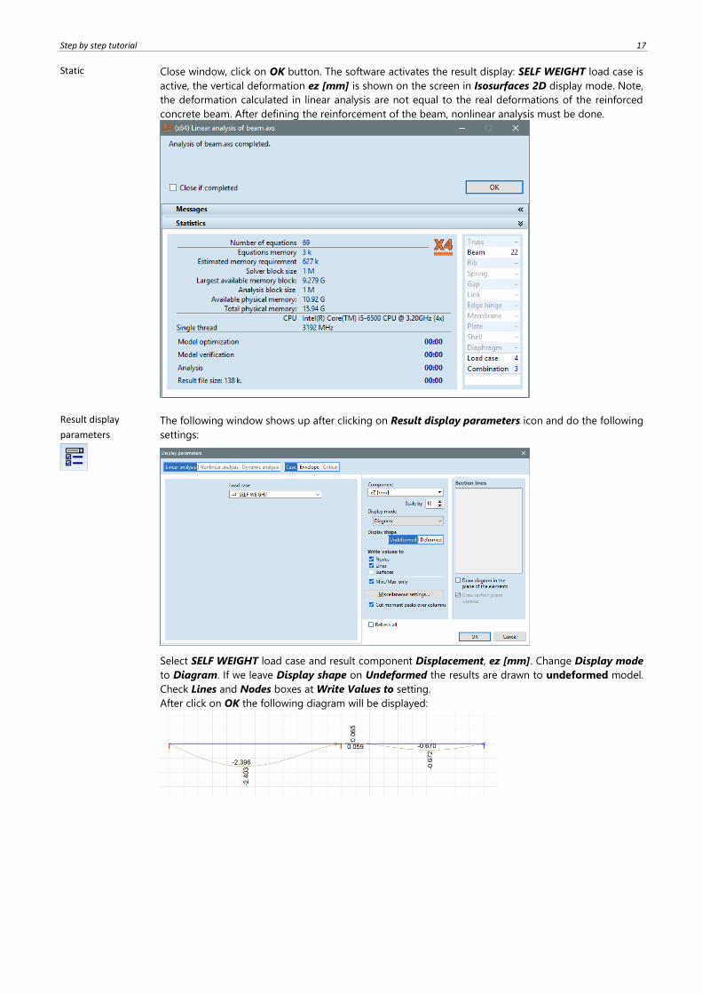
Static Close window, click on OK button. The software activates the result display: SELF WEIGHT load case is
active, the vertical deformation ez [mm] is shown on the screen in Isosurfaces 2D display mode. Note,
the deformation calculated in linear analysis are not equal to the real deformations of the reinforced
concrete beam. After defining the reinforcement of the beam, nonlinear analysis must be done.
Result display
parameters
The following window shows up after clicking on Result display parameters icon and do the following
settings:
Select SELF WEIGHT load case and result component Displacement, ez [mm]. Change Display mode
to Diagram. If we leave Display shape on Undeformed the results are drawn to undeformed model.
Check Lines and Nodes boxes at Write Values to setting.
After click on OK the following diagram will be displayed:
18
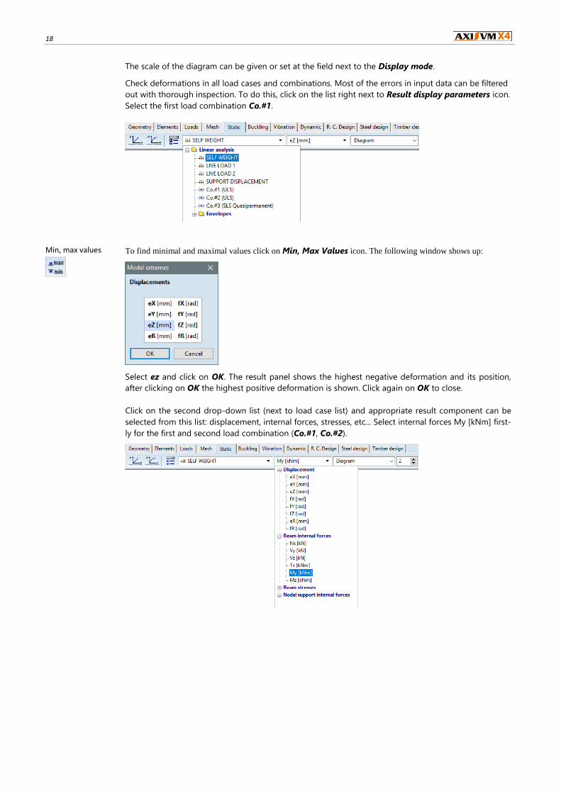
The scale of the diagram can be given or set at the field next to the Display mode.
Check deformations in all load cases and combinations. Most of the errors in input data can be filtered
out with thorough inspection. To do this, click on the list right next to Result display parameters icon.
Select the first load combination Co.#1.
Min, max values
To find minimal and maximal values click on Min, Max Values icon. The following window shows up:
Select ez and click on OK. The result panel shows the highest negative deformation and its position,
after clicking on OK the highest positive deformation is shown. Click again on OK to close.
Click on the second drop-down list (next to load case list) and appropriate result component can be
selected from this list: displacement, internal forces, stresses, etc... Select internal forces My [kNm] first-
ly for the first and second load combination (Co.#1, Co.#2).
Step by step tutorial 19
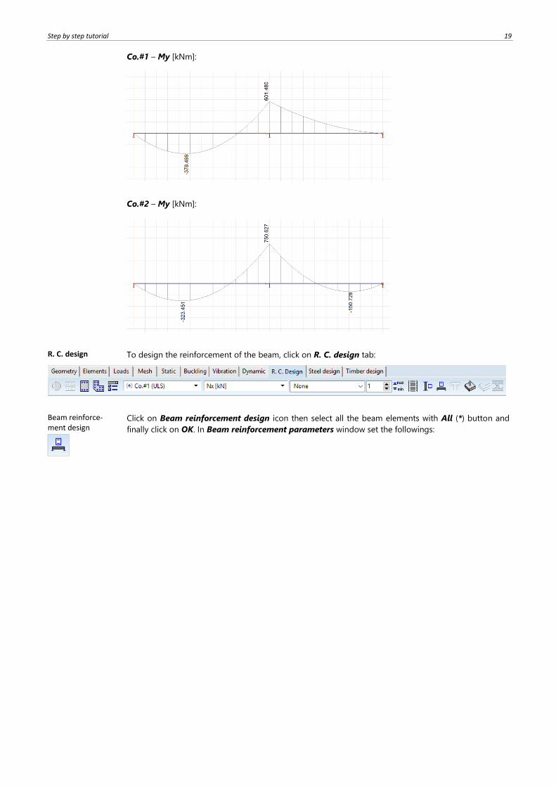
Co.#1 – My [kNm]:
Co.#2 – My [kNm]:
R. C. design To design the reinforcement of the beam, click on R. C. design tab:
Beam reinforce-ment design
Click on Beam reinforcement design icon then select all the beam elements with All (*) button and
finally click on OK. In Beam reinforcement parameters window set the followings:
20
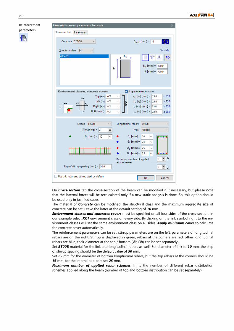
Reinforcement
parameters
On Cross-section tab the cross-section of the beam can be modified if it necessary, but please note
that the internal forces will be recalculated only if a new static analysis is done. So, this option should
be used only in justified cases.
The material of Concrete can be modified, the structural class and the maximum aggregate size of
concrete can be set. Leave the latter at the default setting of 16 mm.
Environment classes and concretes covers must be specified on all four sides of the cross-section. In
our example select XC1 environment class on every side. By clicking on the link symbol right to the en-
vironment classes will set the same environment class on all sides. Apply minimum cover to calculate
the concrete cover automatically.
The reinforcement parameters can be set: stirrup parameters are on the left, parameters of longitudinal
rebars are on the right. Stirrup is displayed in green, rebars at the corners are red, other longitudinal
rebars are blue, their diameter at the top / bottom (Øt, Øb) can be set separately.
Set B500B material for the link and longitudinal rebars as well. Set diameter of link to 10 mm, the step
of stirrup spacing should be the default value of 50 mm.
Set 25 mm for the diameter of bottom longitudinal rebars, but the top rebars at the corners should be
16 mm, for the internal top bars set 25 mm.
Maximum number of applied rebar schemes limits the number of different rebar distribution
schemes applied along the beam (number of top and bottom distribution can be set separately).
Step by step tutorial 21
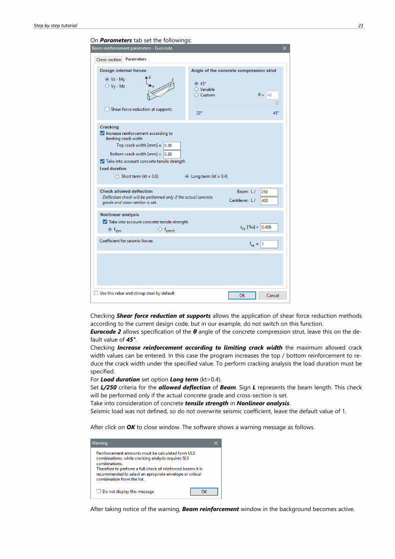
On Parameters tab set the followings:
Checking Shear force reduction at supports allows the application of shear force reduction methods
according to the current design code, but in our example, do not switch on this function.
Eurocode 2 allows specification of the θ angle of the concrete compression strut, leave this on the de-
fault value of 45°.
Checking Increase reinforcement according to limiting crack width the maximum allowed crack
width values can be entered. In this case the program increases the top / bottom reinforcement to re-
duce the crack width under the specified value. To perform cracking analysis the load duration must be
specified.
For Load duration set option Long term (kt=0.4).
Set L/250 criteria for the allowed deflection of Beam. Sign L represents the beam length. This check
will be performed only if the actual concrete grade and cross-section is set.
Take into consideration of concrete tensile strength in Nonlinear analysis.
Seismic load was not defined, so do not overwrite seismic coefficient, leave the default value of 1.
After click on OK to close window. The software shows a warning message as follows.
After taking notice of the warning, Beam reinforcement window in the background becomes active.
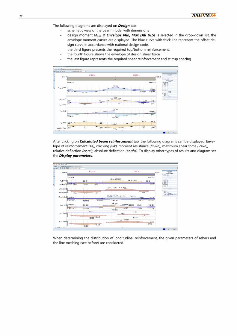
22
The following diagrams are displayed on Design tab:
- schematic view of the beam model with dimensions
- design moment My,Ed. If Envelope Min, Max (All ULS) is selected in the drop-down list, the
envelope moment curves are displayed. The blue curve with thick line represent the offset de-
sign curve in accordance with national design code.
- the third figure presents the required top/bottom reinforcement.
- the fourth figure shows the envelope of design shear force
- the last figure represents the required shear reinforcement and stirrup spacing.
After clicking on Calculated beam reinforcement tab, the following diagrams can be displayed: Enve-
lope of reinforcement (As), cracking (wk), moment resistance (MyRd), maximum shear force (VzRd),
relative deflection (ez,rel), absolute deflection (ez,abs). To display other types of results and diagram set
the Display parameters.
When determining the distribution of longitudinal reinforcement, the given parameters of rebars and
the line meshing (see before) are considered.
Step by step tutorial 23
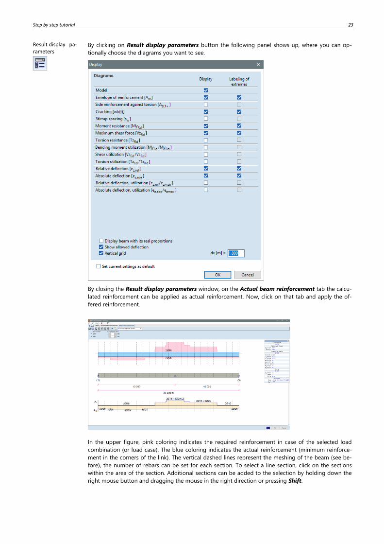
Result display pa-rameters
By clicking on Result display parameters button the following panel shows up, where you can op-
tionally choose the diagrams you want to see.
By closing the Result display parameters window, on the Actual beam reinforcement tab the calcu-
lated reinforcement can be applied as actual reinforcement. Now, click on that tab and apply the of-
fered reinforcement.
In the upper figure, pink coloring indicates the required reinforcement in case of the selected load
combination (or load case). The blue coloring indicates the actual reinforcement (minimum reinforce-
ment in the corners of the link). The vertical dashed lines represent the meshing of the beam (see be-
fore), the number of rebars can be set for each section. To select a line section, click on the sections
within the area of the section. Additional sections can be added to the selection by holding down the
right mouse button and dragging the mouse in the right direction or pressing Shift.

24
The number of the longitudinal reinforcement can be modified. Edit boxes allow changing the number
of top and bottom rebars in the selected elements. The – and + buttons decrease/increase the number
of rebars.
Apply calculated reinforcement
Select Envelope Min, Max (ULS) combination in the dropped-down list next to Apply calculated re-
inforcement icon. The following result will show up:
The software generates the actual reinforcement followings the shape of the internal forces by increas-
ing or decreasing the number of rebars.
If Co.#3 (SLS Quasipermanent) load combination is selected in the drop-down list, the deflection and
crack width can be queried.
Step by step tutorial 25
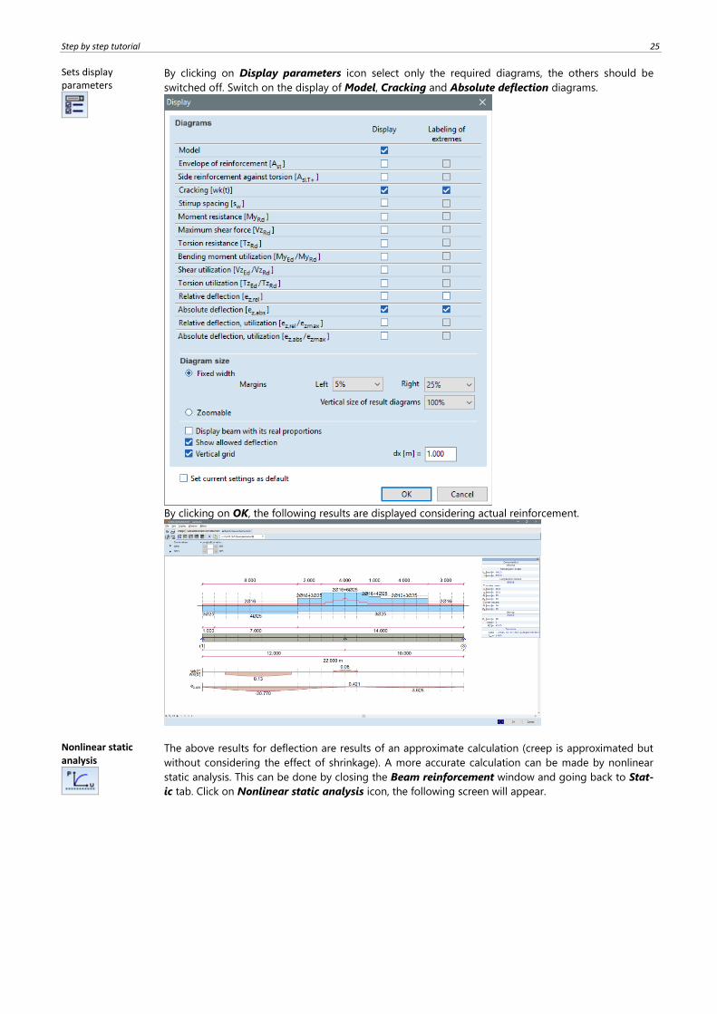
Sets display parameters
By clicking on Display parameters icon select only the required diagrams, the others should be
switched off. Switch on the display of Model, Cracking and Absolute deflection diagrams.
By clicking on OK, the following results are displayed considering actual reinforcement.
Nonlinear static analysis
The above results for deflection are results of an approximate calculation (creep is approximated but
without considering the effect of shrinkage). A more accurate calculation can be made by nonlinear
static analysis. This can be done by closing the Beam reinforcement window and going back to Stat-
ic tab. Click on Nonlinear static analysis icon, the following screen will appear.
26
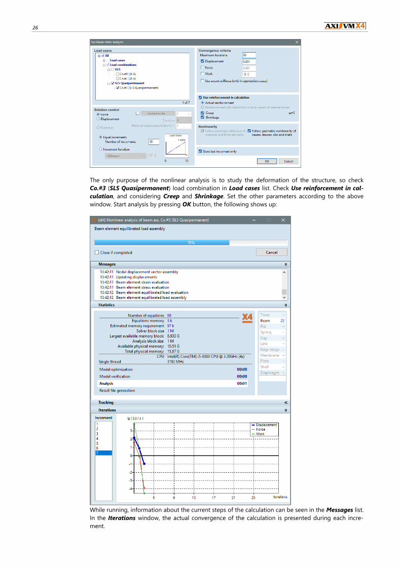
The only purpose of the nonlinear analysis is to study the deformation of the structure, so check
Co.#3 (SLS Quasipermanent) load combination in Load cases list. Check Use reinforcement in cal-
culation, and considering Creep and Shrinkage. Set the other parameters according to the above
window. Start analysis by pressing OK button, the following shows up:
While running, information about the current steps of the calculation can be seen in the Messages list.
In the Iterations window, the actual convergence of the calculation is presented during each incre-
ment.

Step by step tutorial 27
The calculation finishes with the following message:
Finishing the calculation, the result of the nonlinear analysis can be found in the drop-down list.
28
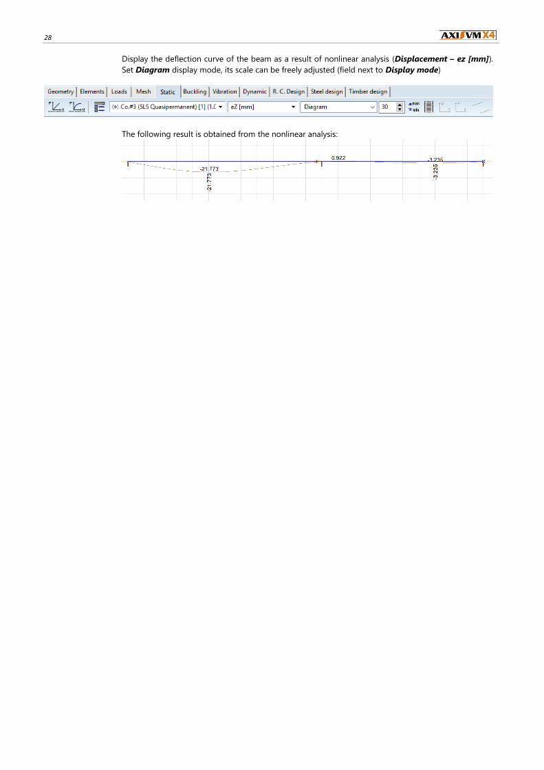
Display the deflection curve of the beam as a result of nonlinear analysis (Displacement – ez [mm]).
Set Diagram display mode, its scale can be freely adjusted (field next to Display mode)
The following result is obtained from the nonlinear analysis:
Step by step tutorial 29
2. FRAME MODEL
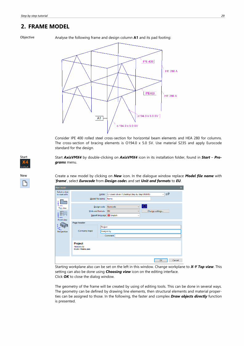
Objective
Analyse the following frame and design column A1 and its pad footing:
Consider IPE 400 rolled steel cross-section for horizontal beam elements and HEA 280 for columns.
The cross-section of bracing elements is O194.0 x 5.0 SV. Use material S235 and apply Eurocode
standard for the design.
Start
Start AxisVMX4 by double-clicking on AxisVMX4 icon in its installation folder, found in Start – Pro-
grams menu.
New
Create a new model by clicking on New icon. In the dialogue window replace Model file name with
‘frame’, select Eurocode from Design codes and set Unit and formats to EU.
Starting workplane also can be set on the left in this window. Change workplane to X-Y Top view. This
setting can also be done using Choosing view icon on the editing interface.
Click OK to close the dialog window.
The geometry of the frame will be created by using of editing tools. This can be done in several ways.
The geometry can be defined by drawing line elements, then structural elements and material proper-
ties can be assigned to those. In the following, the faster and complex Draw objects directly function
is presented.

30
Define of geometry -
Elements
Select Elements tab to bring up Elements toolbar.
Draw objects
directly
Firstly, the columns will be defined. By clicking on Draw objects directly icon shows following win-
dow:
Click on Column icon even it is already selected.
The following window shows after clicking:
Select Browse cross-section libraries… and click on OK. The following window shows up:
Roll down in the list of Cross-section tables by using vertical sliding bar (or roll mouse wheel) and se-
lect HE European wide flange beams, and click on HEA 280 A. Finish with OK.

Step by step tutorial 31
The following message shows up:
Roll down in the list of Materials by using vertical sliding bar (or roll mouse wheel) and click on S235,
then click on OK.
The selected cross-section and material are displayed in the Drawing objects directly window.
Set Height to 3.5 m in the window:
Note: in the window several parameters can be set which are not
mentioned here. End releases can also be specified or the local co-
ordinate system of the element can be modified. In our example, we
use default setting for these. (The end releases of an element are
fixed by default settings.)
Views
Change view to top view (X-Y plane), if it is not the actual view. Note: if necessary, view can be modi-
fied with this icon, even if an editing command is active.
Column
Click on Column icon below to place the columns.
Click on the following positions in the graphical interface:
(0; 0) – (6; 0) – (0; 5) – (6; 5) – (0; 10) – (6; 10).
The next figure shows the result, the columns in X-Y plane view:
32
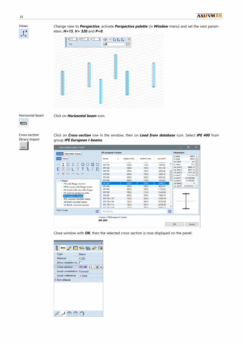
Views
Change view to Perspective, activate Perspective palette (in Window menu) and set the next param-
eters: H=15, V= 320 and P=0:
Horizontal beam
Click on Horizontal beam icon.
Cross-section library import
Click on Cross-section row in the window, then on Load from database icon. Select IPE 400 from
group IPE European I-beams.
Close window with OK, then the selected cross-section is now displayed on the panel:
Step by step tutorial 33
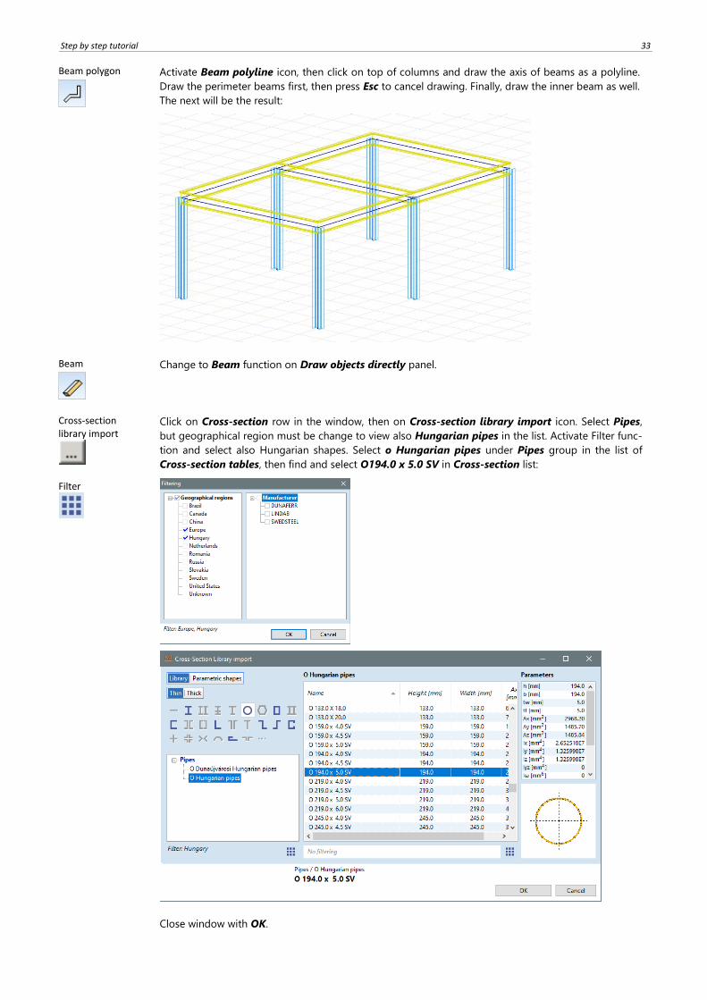
Beam polygon
Activate Beam polyline icon, then click on top of columns and draw the axis of beams as a polyline.
Draw the perimeter beams first, then press Esc to cancel drawing. Finally, draw the inner beam as well.
The next will be the result:
Beam
Change to Beam function on Draw objects directly panel.
Cross-section library import
Filter
Click on Cross-section row in the window, then on Cross-section library import icon. Select Pipes,
but geographical region must be change to view also Hungarian pipes in the list. Activate Filter func-
tion and select also Hungarian shapes. Select o Hungarian pipes under Pipes group in the list of
Cross-section tables, then find and select O194.0 x 5.0 SV in Cross-section list:
Close window with OK.
34
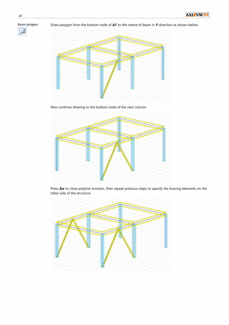
Beam polygon
Draw polygon from the bottom node of A1 to the centre of beam in Y direction as shown below:
then continue drawing to the bottom node of the next column.
Press Esc to close polyline function, then repeat previous steps to specify the bracing elements on the
other side of the structure.
Step by step tutorial 35
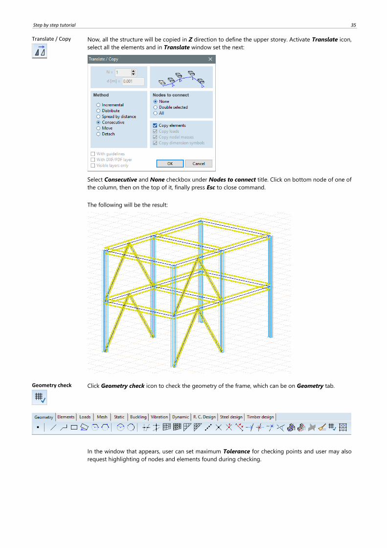
Translate / Copy
Now, all the structure will be copied in Z direction to define the upper storey. Activate Translate icon,
select all the elements and in Translate window set the next:
Select Consecutive and None checkbox under Nodes to connect title. Click on bottom node of one of
the column, then on the top of it, finally press Esc to close command.
The following will be the result:
Geometry check
Click Geometry check icon to check the geometry of the frame, which can be on Geometry tab.
In the window that appears, user can set maximum Tolerance for checking points and user may also
request highlighting of nodes and elements found during checking.
36
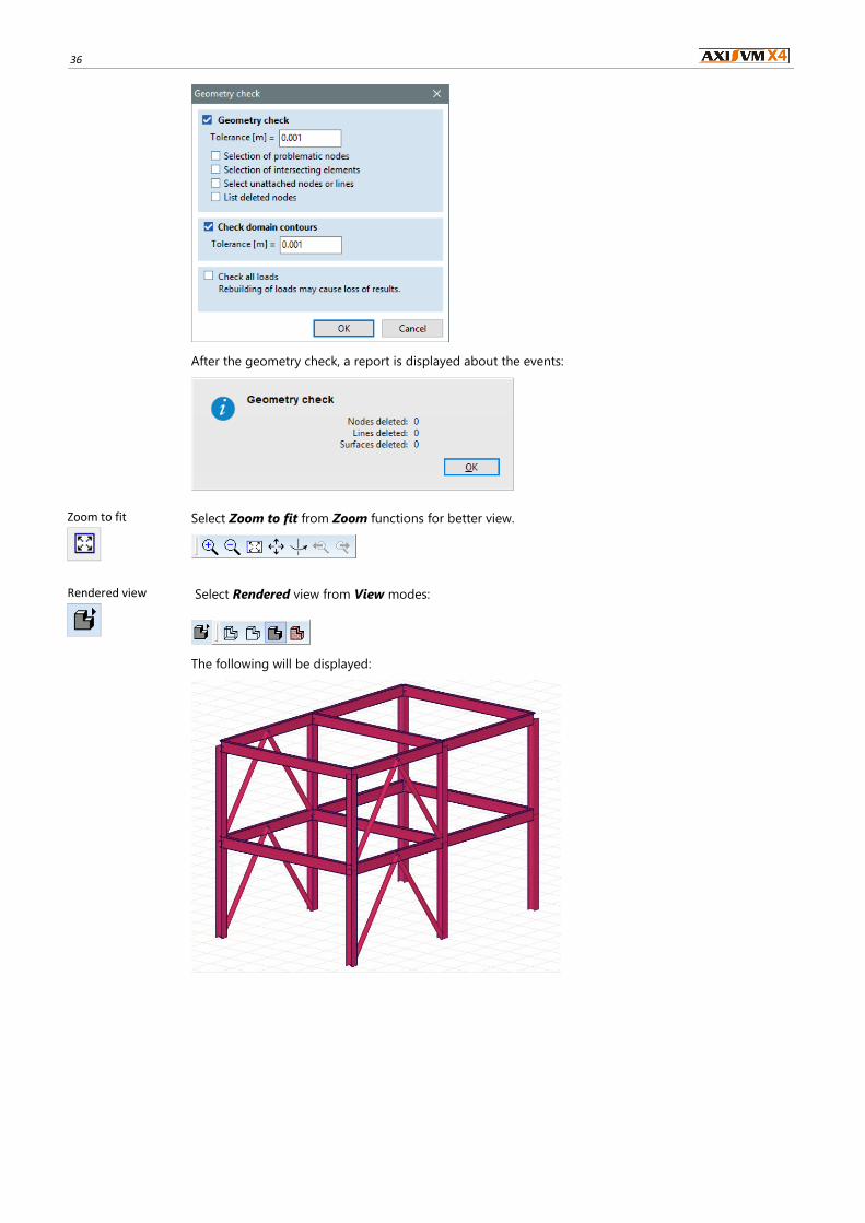
After the geometry check, a report is displayed about the events:
Zoom to fit
Select Zoom to fit from Zoom functions for better view.
Rendered view
Select Rendered view from View modes:
The following will be displayed:

Step by step tutorial 37
Display options
Activate Display options and uncheck Object contours in 3D on Symbols tab.
Wireframe view
Change back to Wireframe view:
Elements To create nodal supports change tab to Elements:
Nodal support
Click on Nodal support icon and select bottom nodes of columns, then confirm with OK. In the next
window the stiffness can be set for the supports:

38
Set rotational stiffness components to 0, but leave translational stiffness on default value (1E+10), as
shown below:
then close window with OK.
Loads To specify the loads on the frame, change tab to Loads:
Load cases and
load groups
Various loads should be separated into load cases. Click on Load cases and load groups icon to add
new load cases.

Step by step tutorial 39
In the window that appears, click on the name ST1 in the top left corner and rename it to LIVE 1. (ST1
is an automatically generated load case, which should be renamed in our example.) Close window with
OK, then the previously edited load case (LIVE LOAD 1) is active. The actual load case is indicated on
Info palette, shown below:
Load along line
elements
Add line loads to all horizontal beams. Specify 50 kN/m to beams at lower level and 25 kN/m to
beams at upper level in -Z direction. Activate the Load along line elements function and select upper
beams with selection rectangle.
Confirm selection with OK, then in the following window set load parameters.
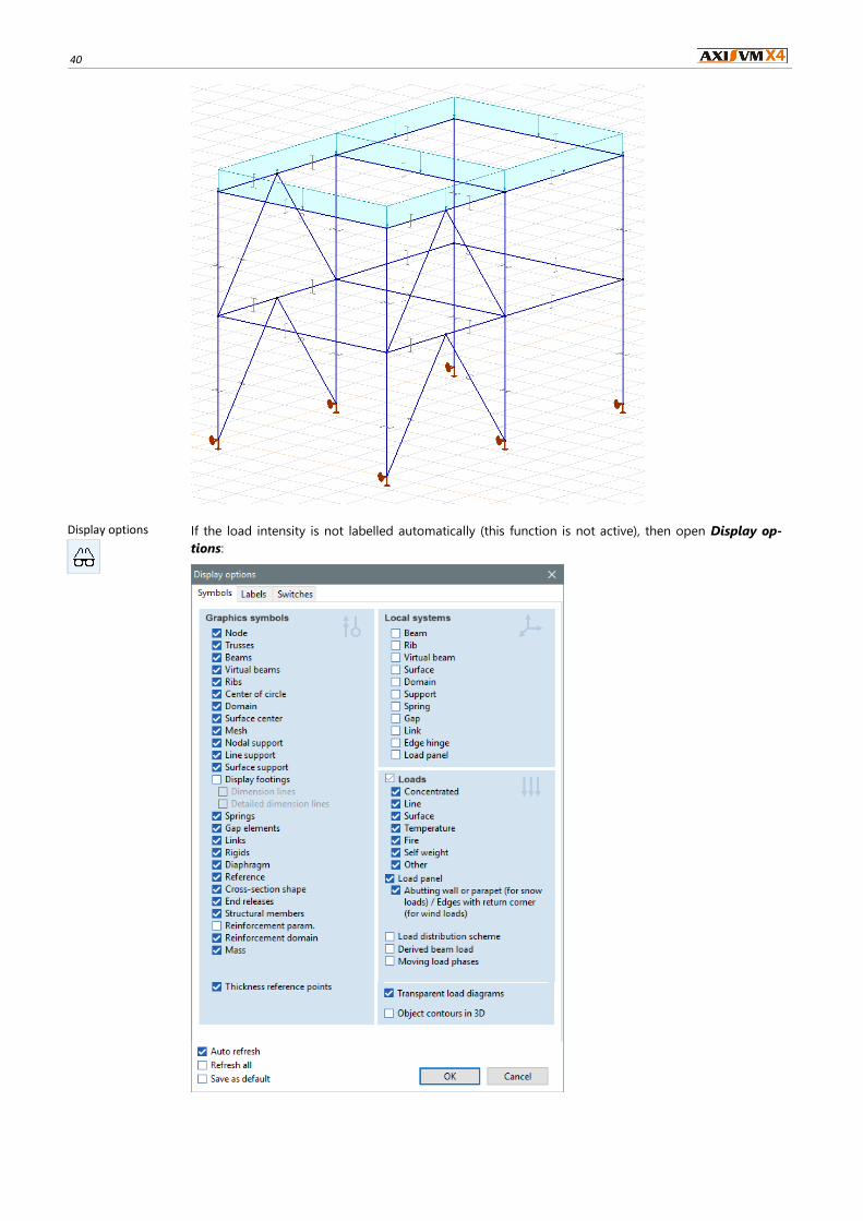
Set pZ1 and pZ2 to –25, then finish with OK, then the load is indicated on the beam elements in cyan:
40
Display options
If the load intensity is not labelled automatically (this function is not active), then open Display op-
tions:
Step by step tutorial 41
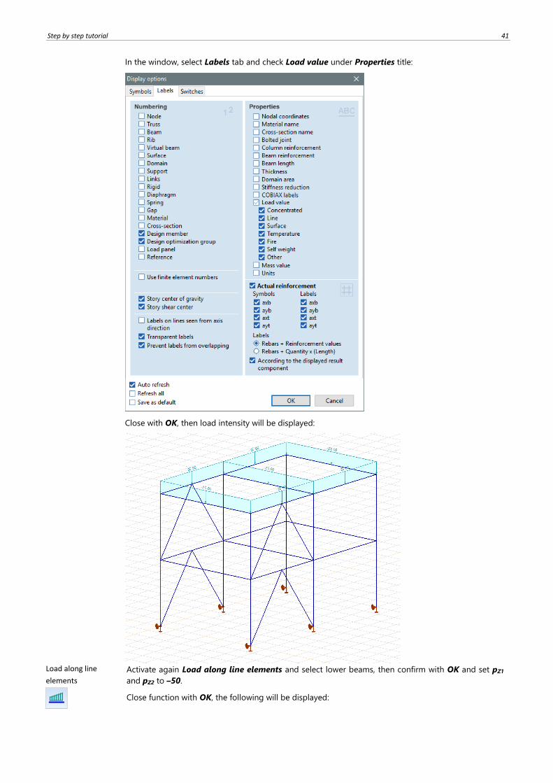
In the window, select Labels tab and check Load value under Properties title:
Close with OK, then load intensity will be displayed:
Load along line
elements
Activate again Load along line elements and select lower beams, then confirm with OK and set pZ1
and pZ2 to –50.
Close function with OK, the following will be displayed:
42
Load cases and
load groups
Click on Load cases and load groups icon.
Static load case
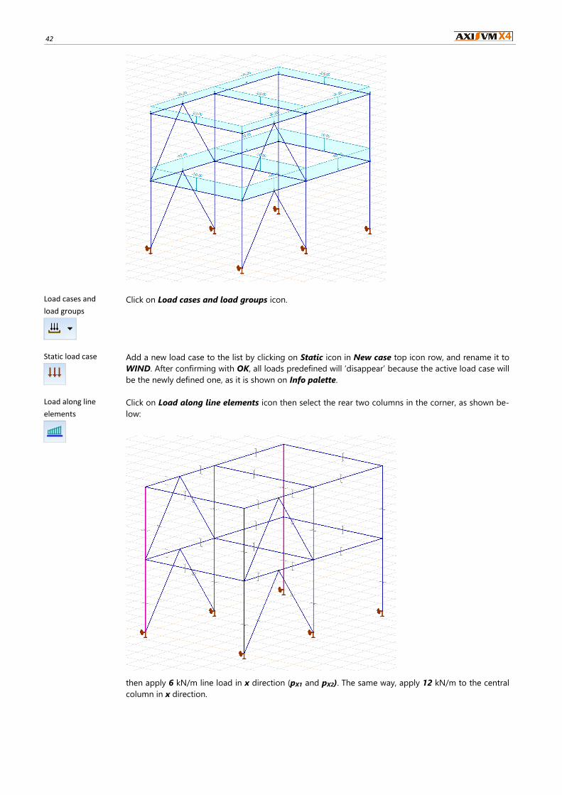
Add a new load case to the list by clicking on Static icon in New case top icon row, and rename it to
WIND. After confirming with OK, all loads predefined will ‘disappear’ because the active load case will
be the newly defined one, as it is shown on Info palette.
Load along line
elements
Click on Load along line elements icon then select the rear two columns in the corner, as shown be-
low:
then apply 6 kN/m line load in x direction (pX1 and pX2). The same way, apply 12 kN/m to the central
column in x direction.
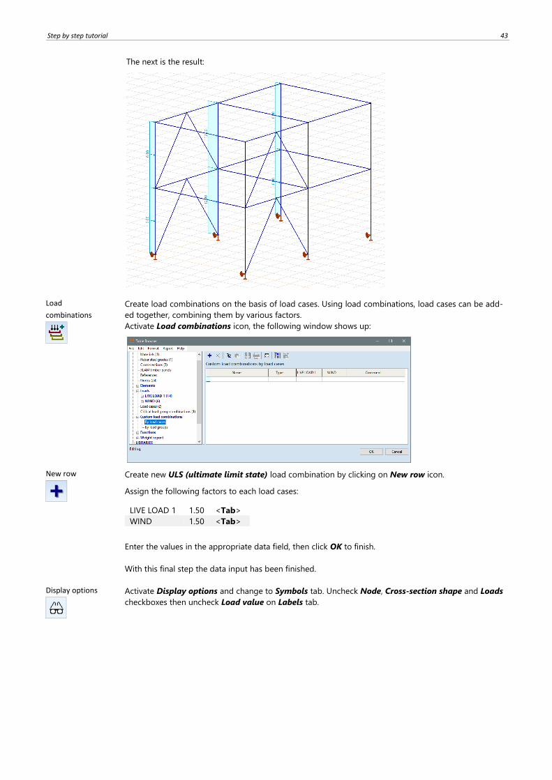
Step by step tutorial 43
The next is the result:
Load
combinations
Create load combinations on the basis of load cases. Using load combinations, load cases can be add-
ed together, combining them by various factors.
Activate Load combinations icon, the following window shows up:
New row
Create new ULS (ultimate limit state) load combination by clicking on New row icon.
Assign the following factors to each load cases:
LIVE LOAD 1 1.50 <Tab>
WIND 1.50 <Tab>
Enter the values in the appropriate data field, then click OK to finish.
With this final step the data input has been finished.
Display options
Activate Display options and change to Symbols tab. Uncheck Node, Cross-section shape and Loads
checkboxes then uncheck Load value on Labels tab.
44
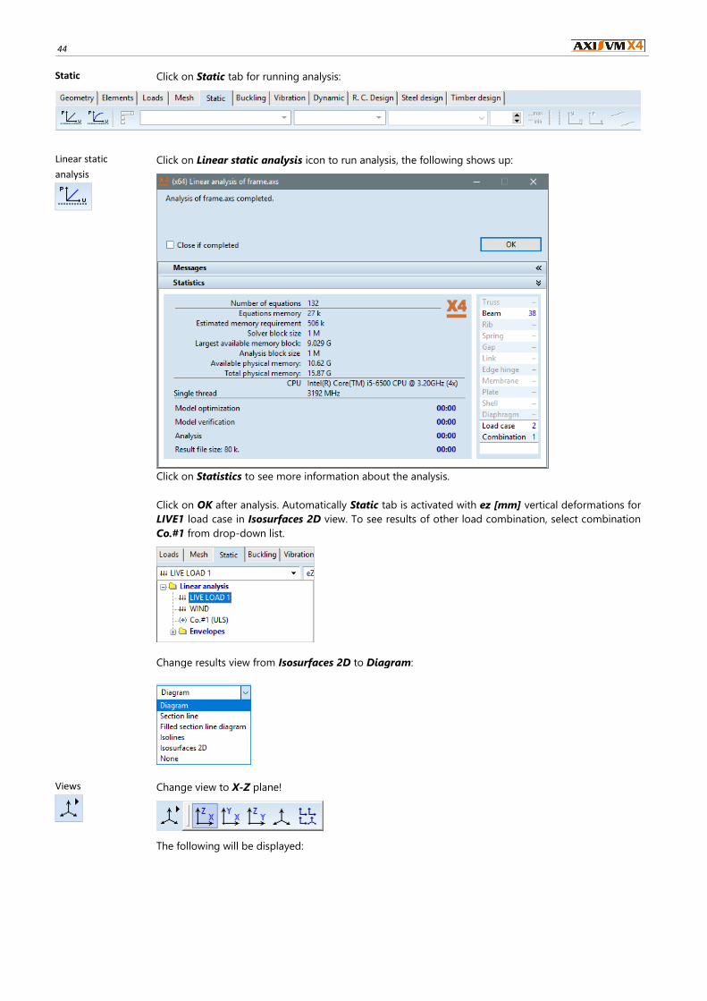
Static Click on Static tab for running analysis:
Linear static
analysis
Click on Linear static analysis icon to run analysis, the following shows up:
Click on Statistics to see more information about the analysis.
Click on OK after analysis. Automatically Static tab is activated with ez [mm] vertical deformations for
LIVE1 load case in Isosurfaces 2D view. To see results of other load combination, select combination
Co.#1 from drop-down list.
Change results view from Isosurfaces 2D to Diagram:
Views
Change view to X-Z plane!
The following will be displayed:
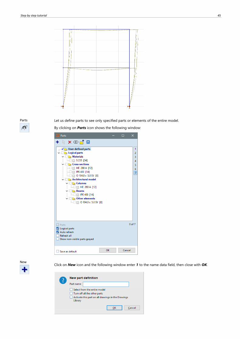
Step by step tutorial 45
Parts
Let us define parts to see only specified parts or elements of the entire model.
By clicking on Parts icon shows the following window:
New
Click on New icon and the following window enter 1 to the name data field, then close with OK.
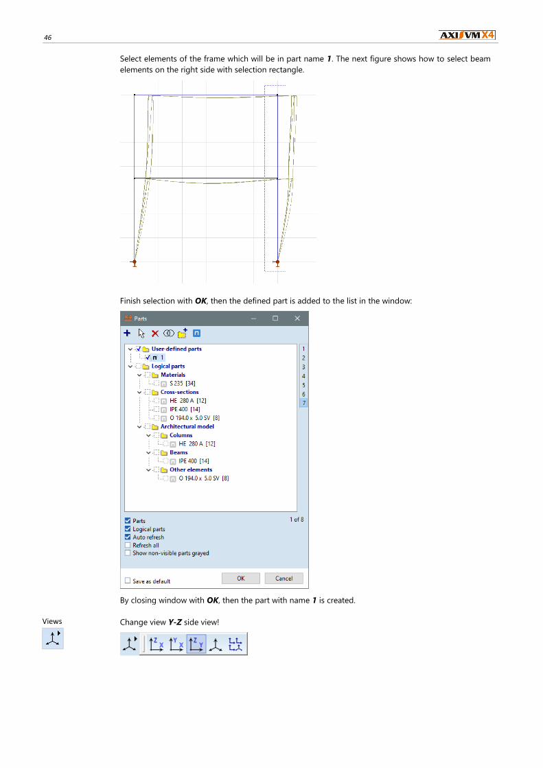
46
Select elements of the frame which will be in part name 1. The next figure shows how to select beam
elements on the right side with selection rectangle.
Finish selection with OK, then the defined part is added to the list in the window:
By closing window with OK, then the part with name 1 is created.
Views
Change view Y-Z side view!
Step by step tutorial 47
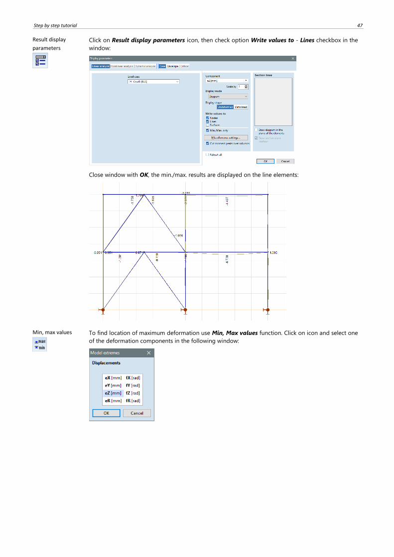
Result display
parameters
Click on Result display parameters icon, then check option Write values to - Lines checkbox in the
window:
Close window with OK, the min./max. results are displayed on the line elements:
Min, max values
To find location of maximum deformation use Min, Max values function. Click on icon and select one
of the deformation components in the following window:
48
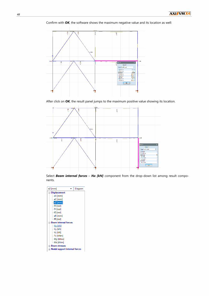
Confirm with OK, the software shows the maximum negative value and its location as well:
After click on OK, the result panel jumps to the maximum positive value showing its location.
Select Beam internal forces – Nx [kN] component from the drop-down list among result compo-
nents.
Step by step tutorial 49
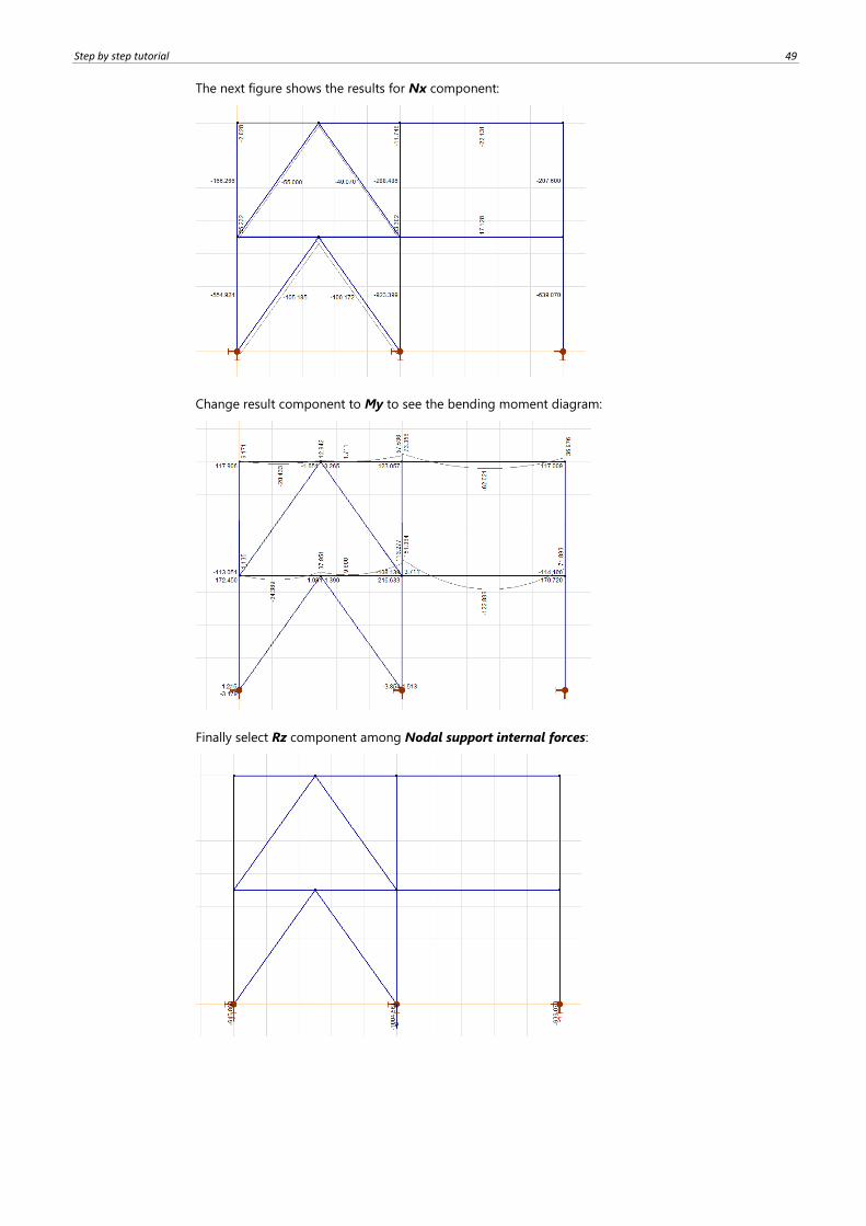
The next figure shows the results for Nx component:
Change result component to My to see the bending moment diagram:
Finally select Rz component among Nodal support internal forces:
50
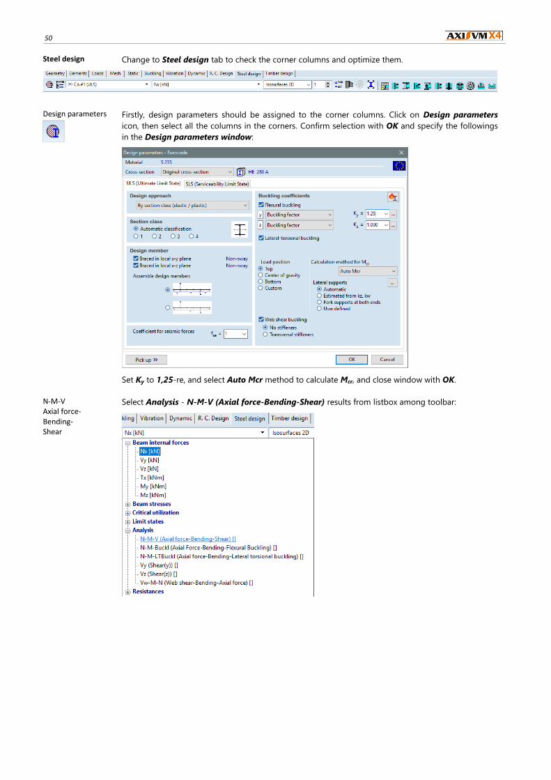
Steel design Change to Steel design tab to check the corner columns and optimize them.
Design parameters
Firstly, design parameters should be assigned to the corner columns. Click on Design parameters
icon, then select all the columns in the corners. Confirm selection with OK and specify the followings
in the Design parameters window:
Set Ky to 1,25-re, and select Auto Mcr method to calculate Mcr, and close window with OK.
N-M-V Axial force- Bending- Shear
Select Analysis - N-M-V (Axial force-Bending-Shear) results from listbox among toolbar:
Step by step tutorial 51
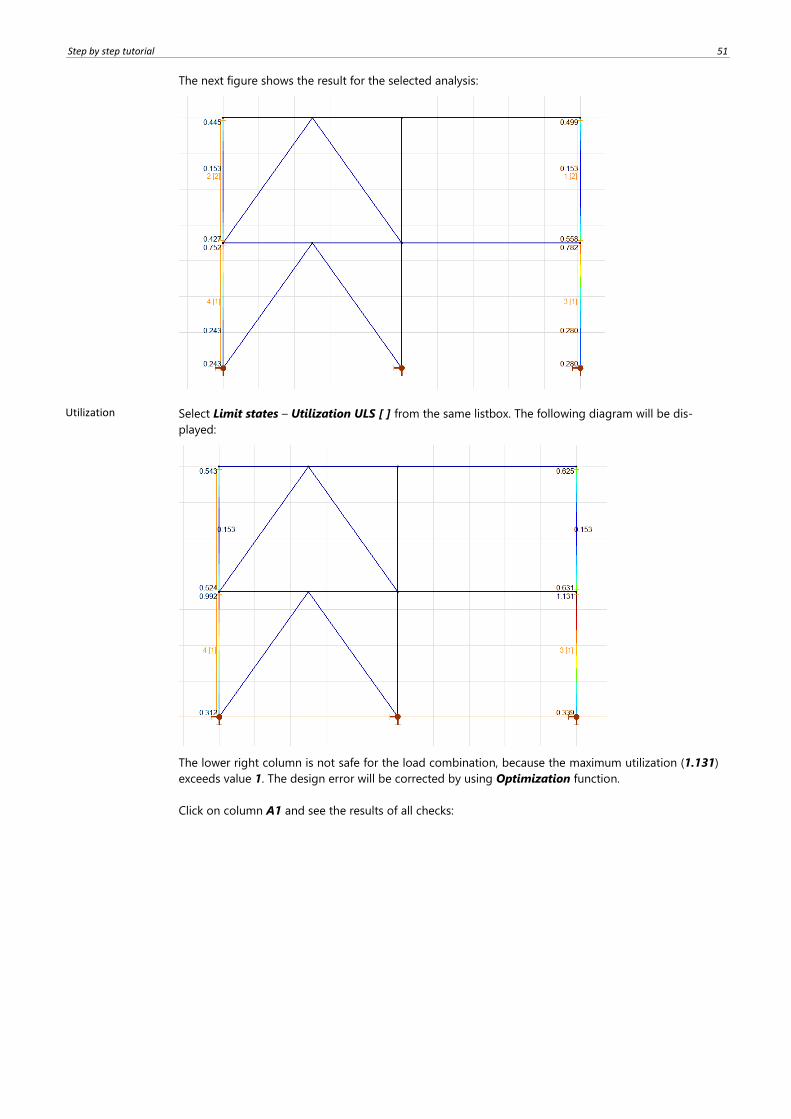
The next figure shows the result for the selected analysis:
Utilization Select Limit states – Utilization ULS [ ] from the same listbox. The following diagram will be dis-
played:
The lower right column is not safe for the load combination, because the maximum utilization (1.131)
exceeds value 1. The design error will be corrected by using Optimization function.
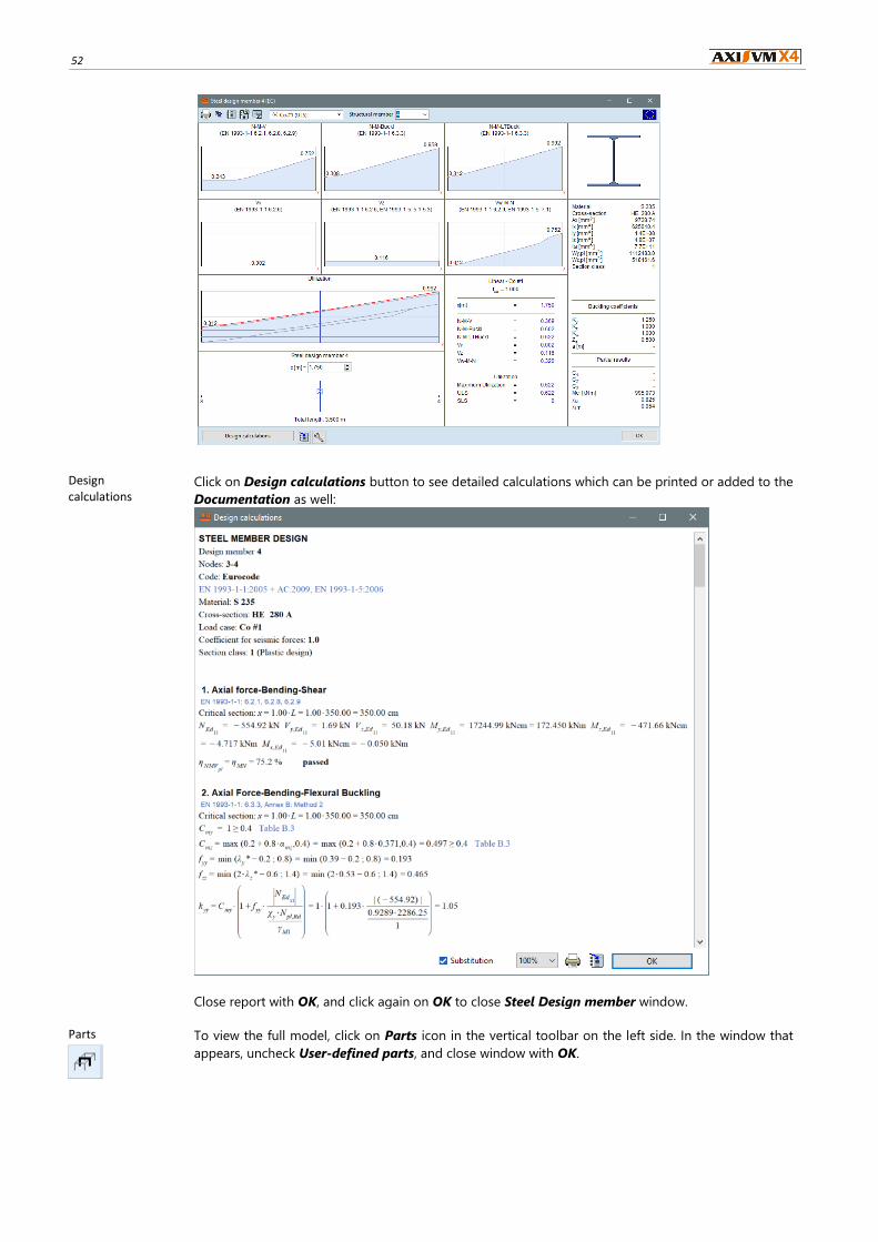
Click on column A1 and see the results of all checks:
52
Design calculations
Click on Design calculations button to see detailed calculations which can be printed or added to the
Documentation as well:
Close report with OK, and click again on OK to close Steel Design member window.
Parts
To view the full model, click on Parts icon in the vertical toolbar on the left side. In the window that
appears, uncheck User-defined parts, and close window with OK.
Step by step tutorial 53
Views
Change view to Perspective!
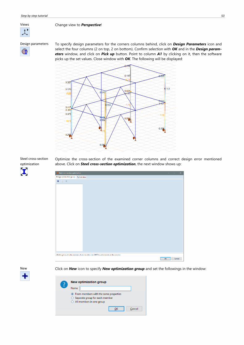
Design parameters
To specify design parameters for the corners columns behind, click on Design Parameters icon and
select the four columns (2 on top, 2 on bottom). Confirm selection with OK and in the Design param-
eters window, and click on Pick up button. Point to column A1 by clicking on it, then the software
picks up the set values. Close window with OK. The following will be displayed:
Steel cross-section
optimization
Optimize the cross-section of the examined corner columns and correct design error mentioned
above. Click on Steel cross-section optimization, the next window shows up:
New
Click on New icon to specify New optimization group and set the followings in the window:
54
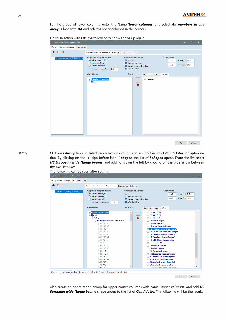
For the group of lower columns, enter the Name ‘lower columns’ and select All members in one
group. Close with OK and select 4 lower columns in the corners.
Finish selection with OK, the following window shows up again:
Library
Click on Library tab and select cross-section groups, and add to the list of Candidates for optimiza-
tion. By clicking on the ‘+’ sign before label I-shapes, the list of I shapes opens. From the list select
HE European wide flange beams, and add to list on the left by clicking on the blue arrow between
the two listboxes.
The following can be seen after setting:
Also create an optimization group for upper corner columns with name ‘upper columns’ and add HE
European wide flange beams shape group to the list of Candidates. The following will be the result:
Step by step tutorial 55
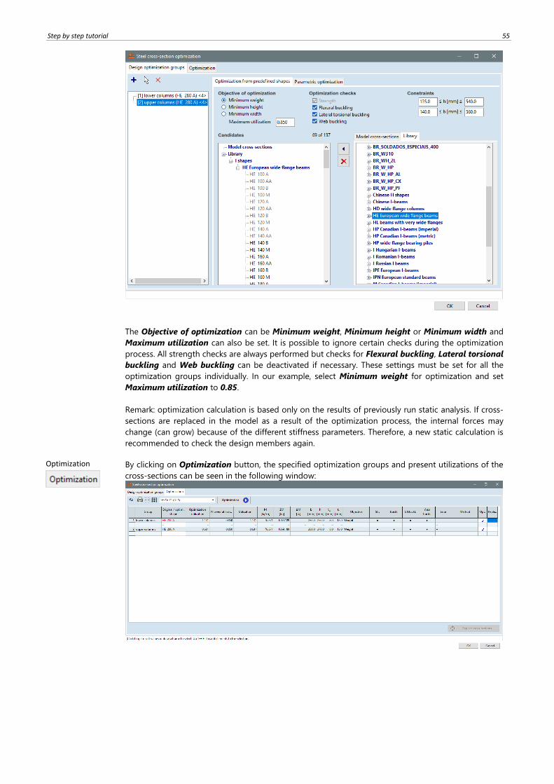
The Objective of optimization can be Minimum weight, Minimum height or Minimum width and
Maximum utilization can also be set. It is possible to ignore certain checks during the optimization
process. All strength checks are always performed but checks for Flexural buckling, Lateral torsional
buckling and Web buckling can be deactivated if necessary. These settings must be set for all the
optimization groups individually. In our example, select Minimum weight for optimization and set
Maximum utilization to 0.85.
Remark: optimization calculation is based only on the results of previously run static analysis. If cross-
sections are replaced in the model as a result of the optimization process, the internal forces may
change (can grow) because of the different stiffness parameters. Therefore, a new static calculation is
recommended to check the design members again.
Optimization
By clicking on Optimization button, the specified optimization groups and present utilizations of the
cross-sections can be seen in the following window:
56
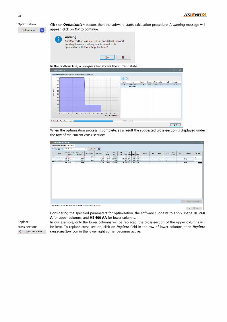
Optimization
Click on Optimization button, then the software starts calculation procedure. A warning message will
appear, click on OK to continue.
In the bottom line, a progress bar shows the current state.
When the optimization process is complete, as a result the suggested cross-section is displayed under
the row of the current cross-section:
Considering the specified parameters for optimization, the software suggests to apply shape HE 260
A for upper columns, and HE 400 AA for lower columns.
Replace
cross-sections
In our example, only the lower columns will be replaced, the cross-section of the upper columns will
be kept. To replace cross-section, click on Replace field in the row of lower columns, then Replace
cross-section icon in the lower right corner becomes active:

Step by step tutorial 57
Activate Replacing cross-section icon, then software offers to save the model under a new name be-
fore replacing cross-sections:
Click on No, keep the original file name.
In the following window click on Yes:
Changing the model by replacing cross-sections, the model must be saved and previous results of
static analysis will be deleted.
Linear static
analysis
On Static tab, run a new Linear static analysis.
58
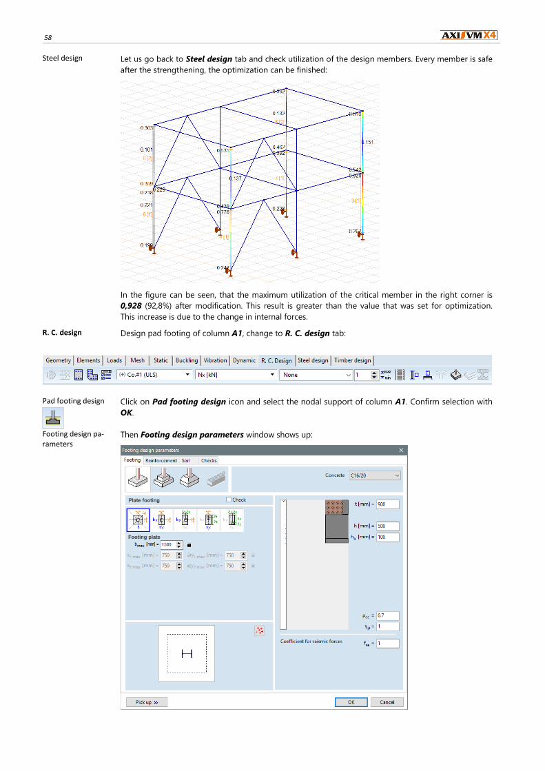
Steel design Let us go back to Steel design tab and check utilization of the design members. Every member is safe
after the strengthening, the optimization can be finished:
In the figure can be seen, that the maximum utilization of the critical member in the right corner is
0,928 (92,8%) after modification. This result is greater than the value that was set for optimization.
This increase is due to the change in internal forces.
R. C. design Design pad footing of column A1, change to R. C. design tab:
Pad footing design
Click on Pad footing design icon and select the nodal support of column A1. Confirm selection with
OK.
Footing design pa-rameters
Then Footing design parameters window shows up:
Step by step tutorial 59
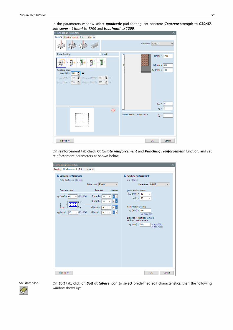
In the parameters window select quadratic pad footing, set concrete Concrete strength to C30/37,
soil cover - t [mm] to 1700 and bmax [mm] to 1200:
On reinforcement tab check Calculate reinforcement and Punching reinforcement function, and set
reinforcement parameters as shown below:
Soil database
On Soil tab, click on Soil database icon to select predefined soil characteristics, then the following
window shows up:
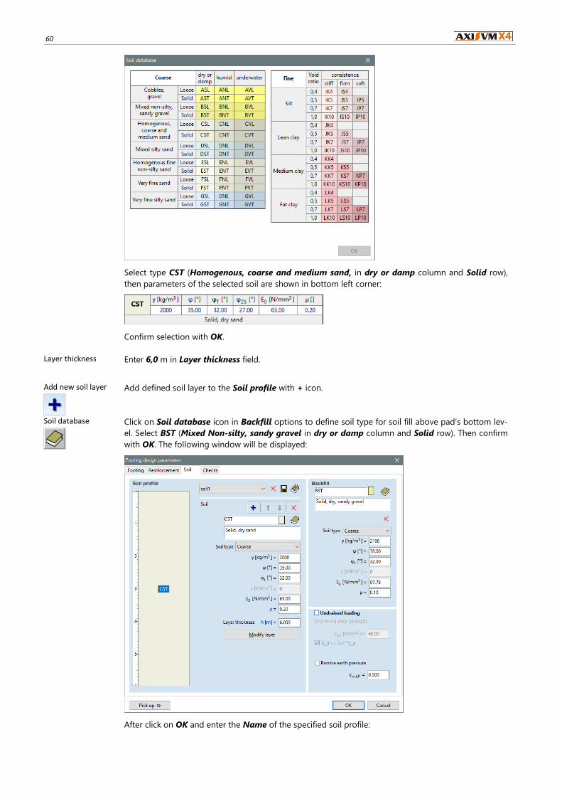
60
Select type CST (Homogenous, coarse and medium sand, in dry or damp column and Solid row),
then parameters of the selected soil are shown in bottom left corner:
Confirm selection with OK.
Layer thickness Enter 6,0 m in Layer thickness field.
Add new soil layer
Add defined soil layer to the Soil profile with + icon.
Soil database
Click on Soil database icon in Backfill options to define soil type for soil fill above pad’s bottom lev-
el. Select BST (Mixed Non-silty, sandy gravel in dry or damp column and Solid row). Then confirm
with OK. The following window will be displayed:
After click on OK and enter the Name of the specified soil profile:
Step by step tutorial 61
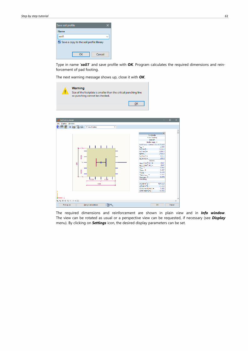
Type in name ‘soil1’ and save profile with OK. Program calculates the required dimensions and rein-
forcement of pad footing.
The next warning message shows up, close it with OK.
The required dimensions and reinforcement are shown in plain view and in Info window.
The view can be rotated as usual or a perspective view can be requested, if necessary (see Display
menu). By clicking on Settings icon, the desired display parameters can be set.
62
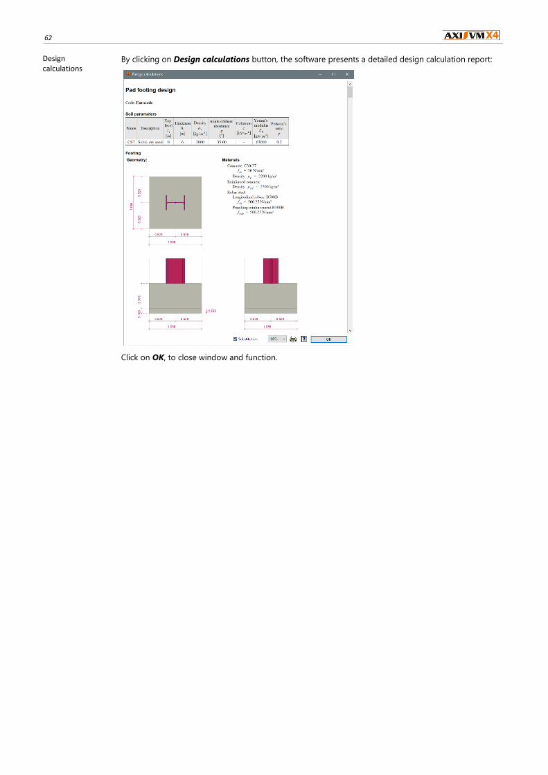
Design calculations
By clicking on Design calculations button, the software presents a detailed design calculation report:
Click on OK, to close window and function.
Step by step tutorial 63
3. SLAB MODEL
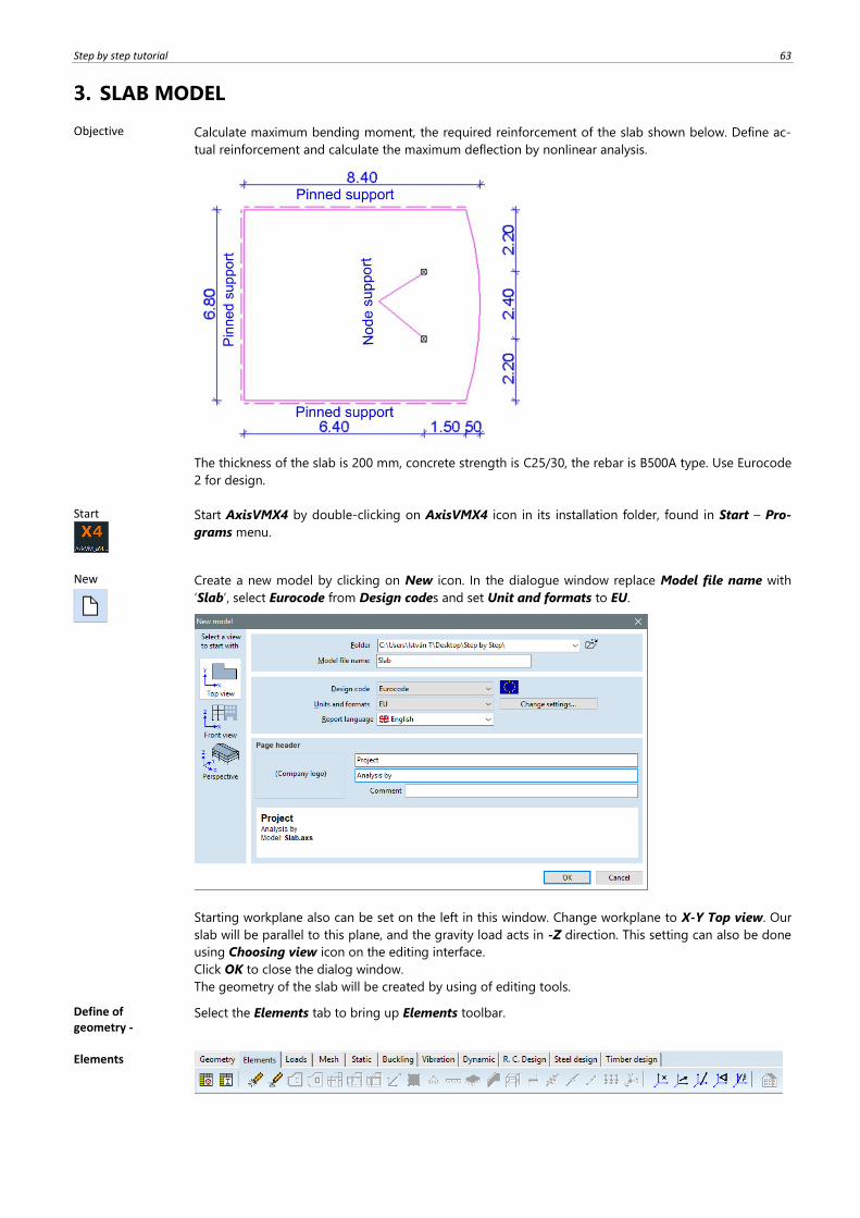
Objective Calculate maximum bending moment, the required reinforcement of the slab shown below. Define ac-
tual reinforcement and calculate the maximum deflection by nonlinear analysis.
The thickness of the slab is 200 mm, concrete strength is C25/30, the rebar is B500A type. Use Eurocode
2 for design.
Start
Start AxisVMX4 by double-clicking on AxisVMX4 icon in its installation folder, found in Start – Pro-
grams menu.
New
Create a new model by clicking on New icon. In the dialogue window replace Model file name with
‘Slab’, select Eurocode from Design codes and set Unit and formats to EU.
Starting workplane also can be set on the left in this window. Change workplane to X-Y Top view. Our
slab will be parallel to this plane, and the gravity load acts in -Z direction. This setting can also be done
using Choosing view icon on the editing interface.
Click OK to close the dialog window.
The geometry of the slab will be created by using of editing tools.
Define of geometry -
Select the Elements tab to bring up Elements toolbar.
Elements
64
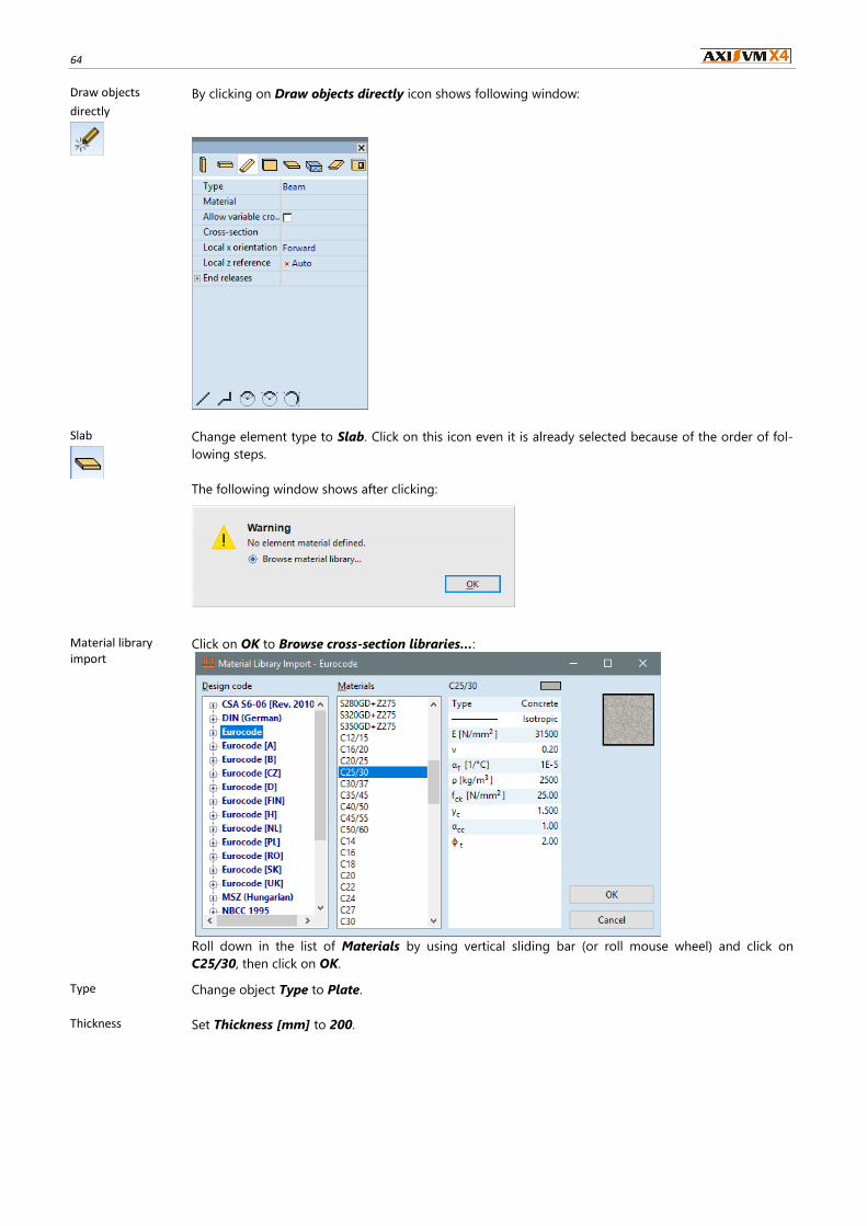
Draw objects
directly
By clicking on Draw objects directly icon shows following window:
Slab
Change element type to Slab. Click on this icon even it is already selected because of the order of fol-
lowing steps.
The following window shows after clicking:
Material library import
Click on OK to Browse cross-section libraries…:
Roll down in the list of Materials by using vertical sliding bar (or roll mouse wheel) and click on
C25/30, then click on OK.
Type Change object Type to Plate.
Thickness Set Thickness [mm] to 200.
Step by step tutorial 65
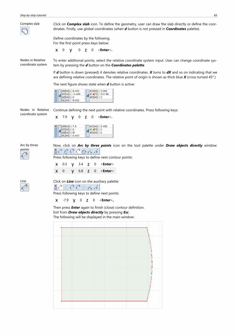
Complex slab
Click on Complex slab icon. To define the geometry, user can draw the slab directly or define the coor-
dinates. Firstly, use global coordinates (when d button is not pressed in Coordinates palette).
Define coordinates by the following.
For the first point press keys below:
x 0 y 0 z 0 <Enter>.
Nodes in Relative coordinate system
To enter additional points, select the relative coordinate system input. User can change coordinate sys-
tem by pressing the d button on the Coordinates palette.
If d button is down (pressed) it denotes relative coordinates. X turns to dX and so on indicating that we
are defining relative coordinates. The relative point of origin is shown as thick blue X (cross turned 45°.)
The next figure shows state when d button is active:
Nodes in Relative coordinate system
Continue defining the next point with relative coordinates. Press following keys:
x 7.9 y 0 z 0 <Enter>.
Arc by three points
Now, click on Arc by three points icon on the tool palette under Draw objects directly window:
Press following keys to define next contour points:
x 0.5 y 3.4 z 0 <Enter>
x 0 y 6.8 z 0 <Enter>
Line
Click on Line icon on the auxiliary palette:
Press following keys to define next points:
Then press Enter again to finish (close) contour definition.
x -7.9 y 0 z 0 <Enter>,
Exit from Draw objects directly by pressing Esc.
The following will be displayed in the main window:
66
To move the origin of the local coordinate system to the bottom left corner of the slab, move cursor to
that position and press Insert key.
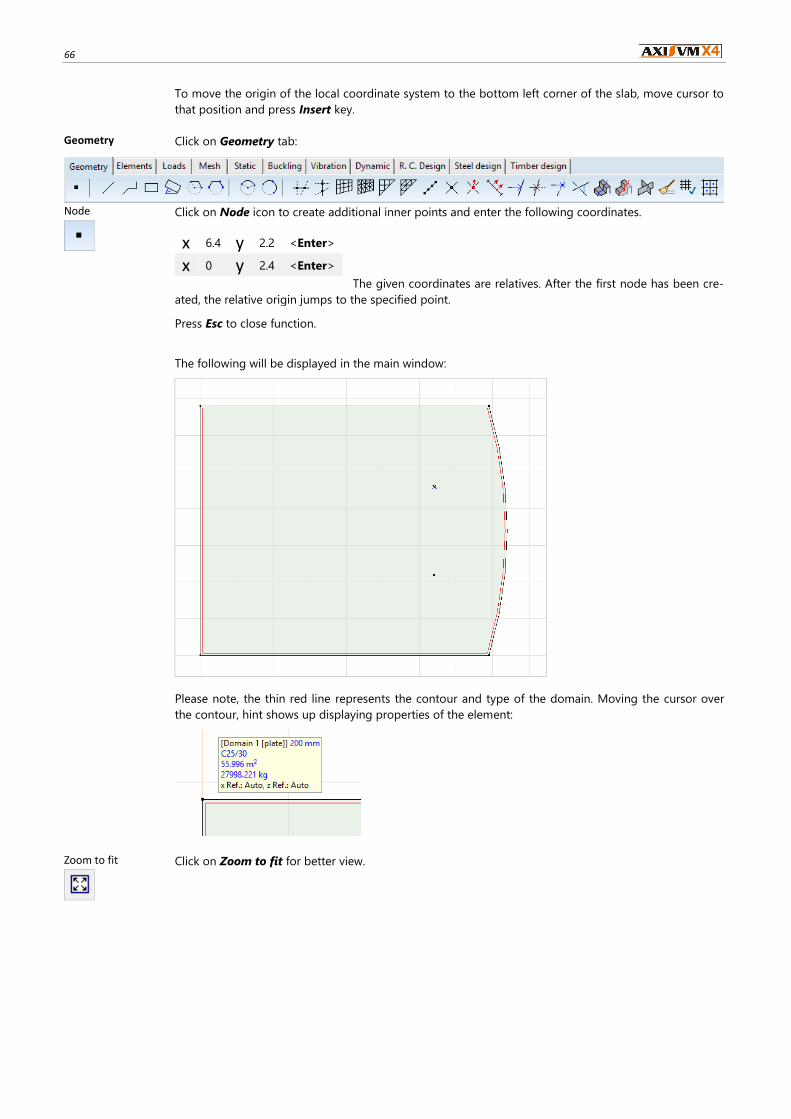
Geometry Click on Geometry tab:
Node
Click on Node icon to create additional inner points and enter the following coordinates.
The given coordinates are relatives. After the first node has been cre-
ated, the relative origin jumps to the specified point.
x 6.4 y 2.2 <Enter>
x 0 y 2.4 <Enter>
Press Esc to close function.
The following will be displayed in the main window:
Please note, the thin red line represents the contour and type of the domain. Moving the cursor over
the contour, hint shows up displaying properties of the element:
Zoom to fit
Click on Zoom to fit for better view.
Step by step tutorial 67
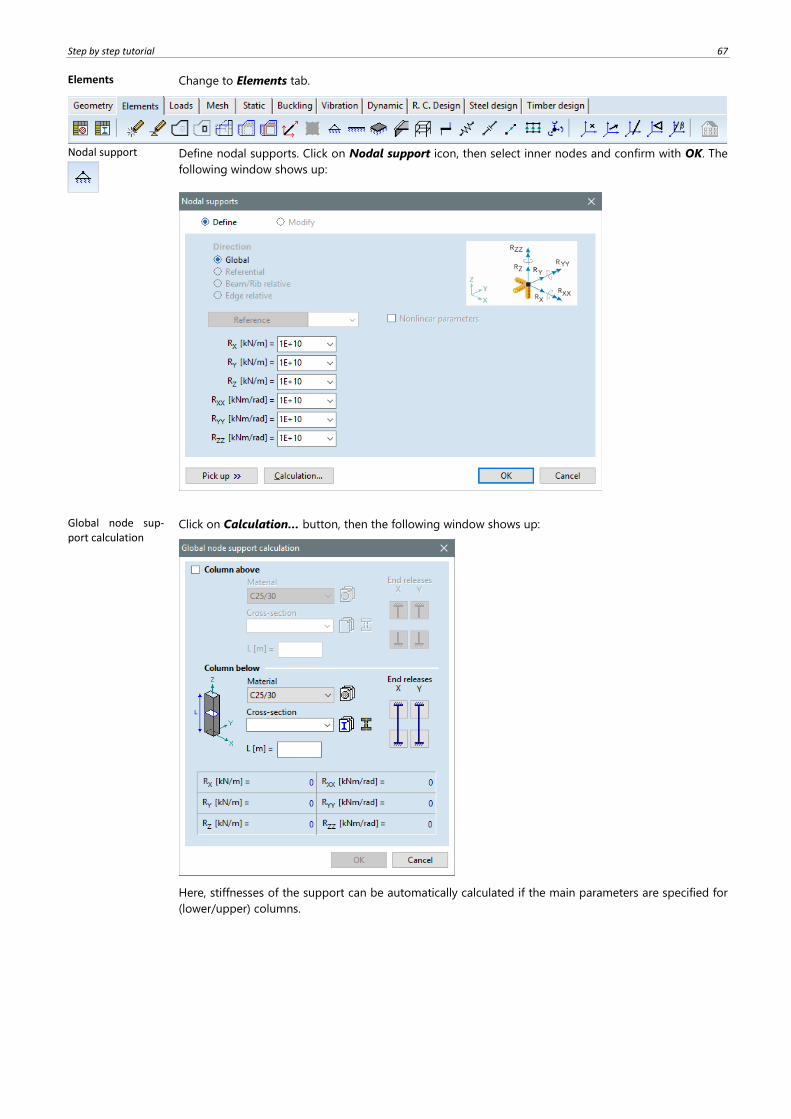
Elements Change to Elements tab.
Nodal support
Define nodal supports. Click on Nodal support icon, then select inner nodes and confirm with OK. The
following window shows up:
Global node sup-port calculation
Click on Calculation… button, then the following window shows up:
Here, stiffnesses of the support can be automatically calculated if the main parameters are specified for
(lower/upper) columns.
68
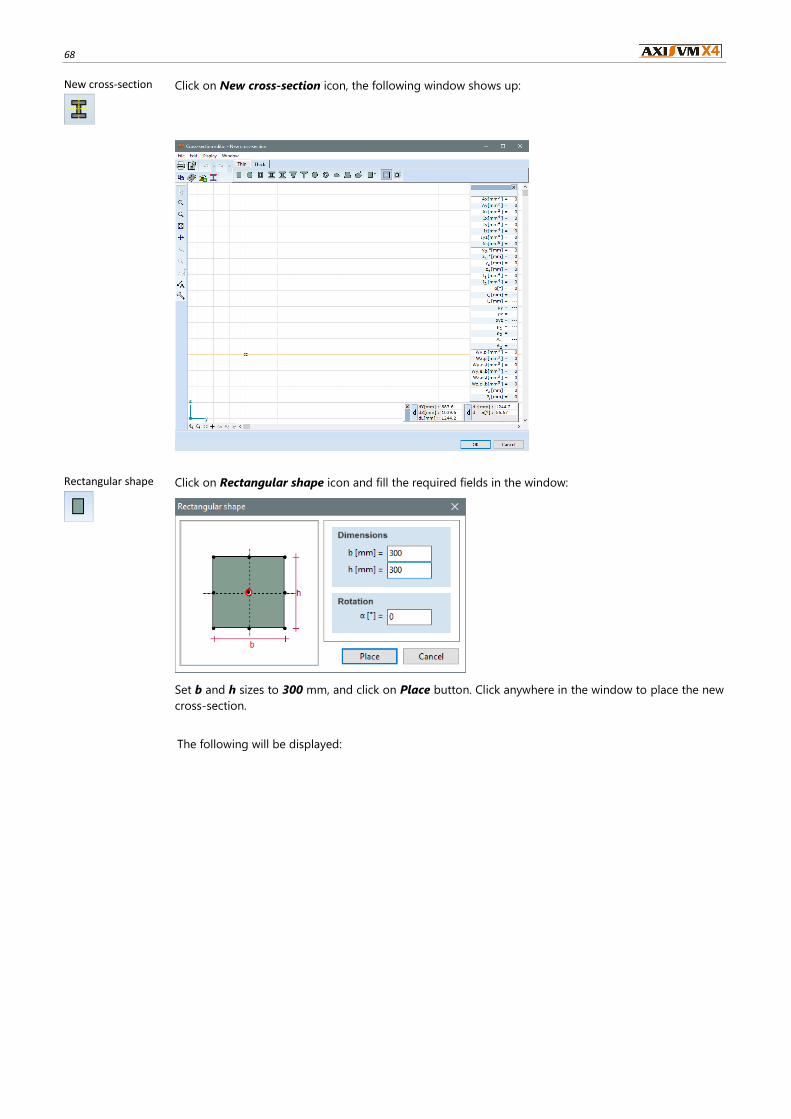
New cross-section
Click on New cross-section icon, the following window shows up:
Rectangular shape
Click on Rectangular shape icon and fill the required fields in the window:
Set b and h sizes to 300 mm, and click on Place button. Click anywhere in the window to place the new
cross-section.
The following will be displayed:
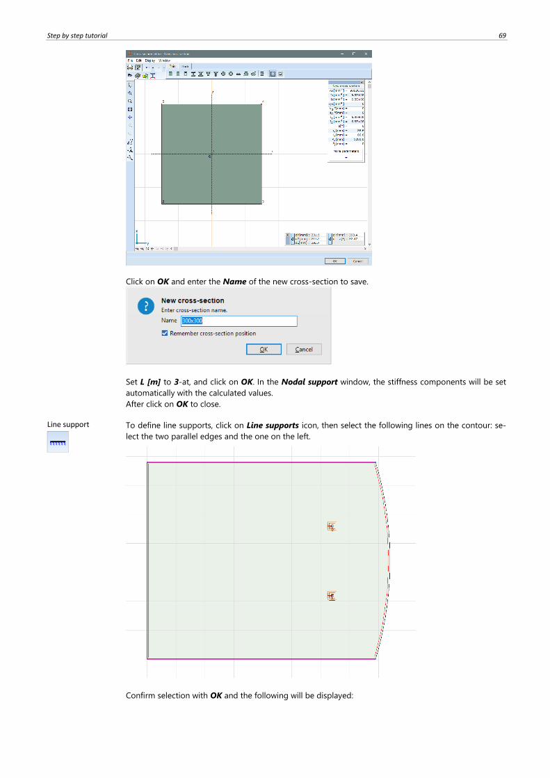
Step by step tutorial 69
Click on OK and enter the Name of the new cross-section to save.
Set L [m] to 3-at, and click on OK. In the Nodal support window, the stiffness components will be set
automatically with the calculated values.
After click on OK to close.
Line support
To define line supports, click on Line supports icon, then select the following lines on the contour: se-
lect the two parallel edges and the one on the left.
Confirm selection with OK and the following will be displayed:

70
Local line support Calculation
Click again on Calculation.. button to calculate the stiffnesses automatically considering support con-
ditions. In the next window set L [m] to 3 and d [m] to 300:
To set End Releases to pinned, click on both icons:
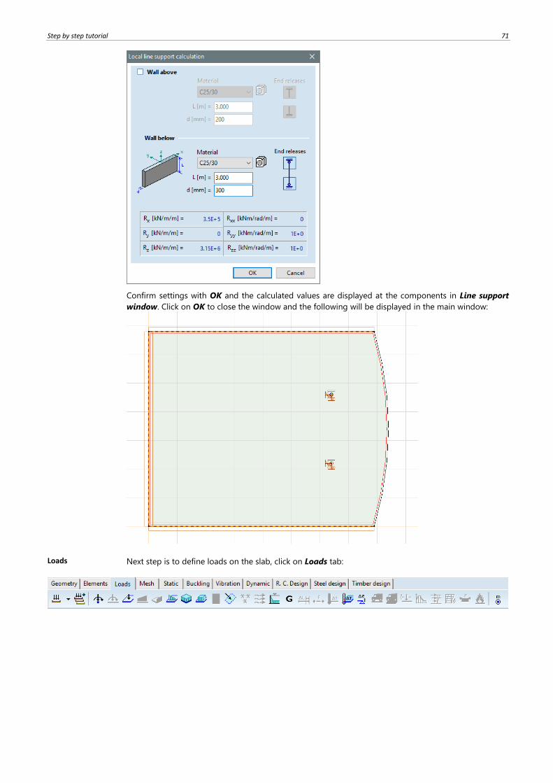
Step by step tutorial 71
Confirm settings with OK and the calculated values are displayed at the components in Line support
window. Click on OK to close the window and the following will be displayed in the main window:
Loads Next step is to define loads on the slab, click on Loads tab:
72
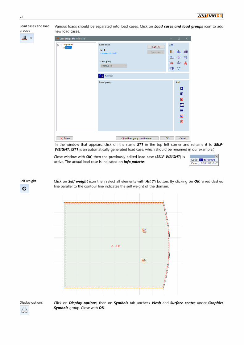
Load cases and load groups
Various loads should be separated into load cases. Click on Load cases and load groups icon to add
new load cases.
In the window that appears, click on the name ST1 in the top left corner and rename it to SELF-
WEIGHT. (ST1 is an automatically generated load case, which should be renamed in our example.)
Close window with OK, then the previously edited load case (SELF-WEIGHT) is
active. The actual load case is indicated on Info palette:
Self weight
Click on Self weight icon then select all elements with All (*) button. By clicking on OK, a red dashed
line parallel to the contour line indicates the self weight of the domain.
Display options
Click on Display options, then on Symbols tab uncheck Mesh and Surface centre under Graphics
Symbols group. Close with OK.
Step by step tutorial 73
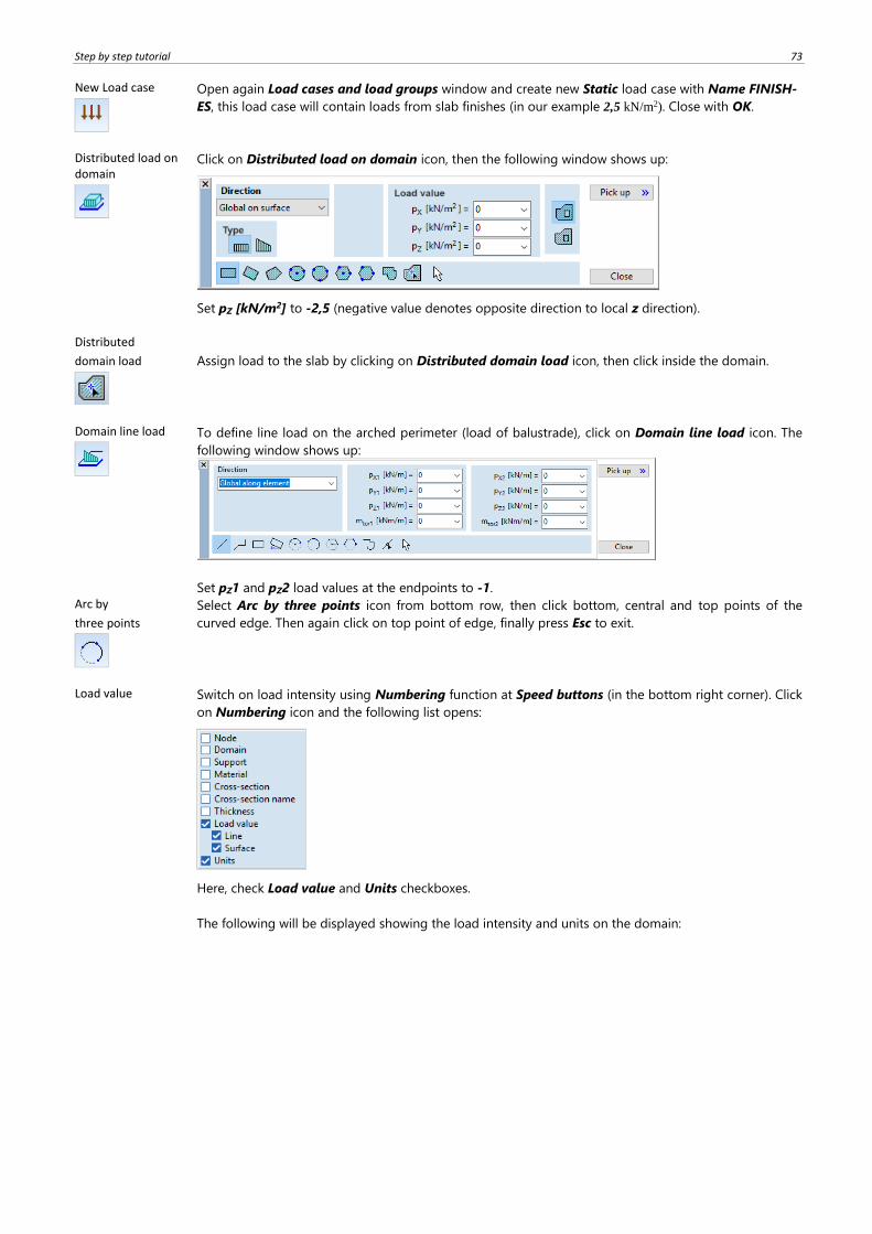
New Load case
Open again Load cases and load groups window and create new Static load case with Name FINISH-
ES, this load case will contain loads from slab finishes (in our example 2,5 kN/m2). Close with OK.
Distributed load on domain
Click on Distributed load on domain icon, then the following window shows up:
Set pZ [kN/m2] to -2,5 (negative value denotes opposite direction to local z direction).
Distributed
domain load
Assign load to the slab by clicking on Distributed domain load icon, then click inside the domain.
Domain line load
To define line load on the arched perimeter (load of balustrade), click on Domain line load icon. The
following window shows up:
Set pZ1 and pZ2 load values at the endpoints to -1.
Arc by
three points
Select Arc by three points icon from bottom row, then click bottom, central and top points of the
curved edge. Then again click on top point of edge, finally press Esc to exit.
Load value Switch on load intensity using Numbering function at Speed buttons (in the bottom right corner). Click
on Numbering icon and the following list opens:
Here, check Load value and Units checkboxes.
The following will be displayed showing the load intensity and units on the domain:
74
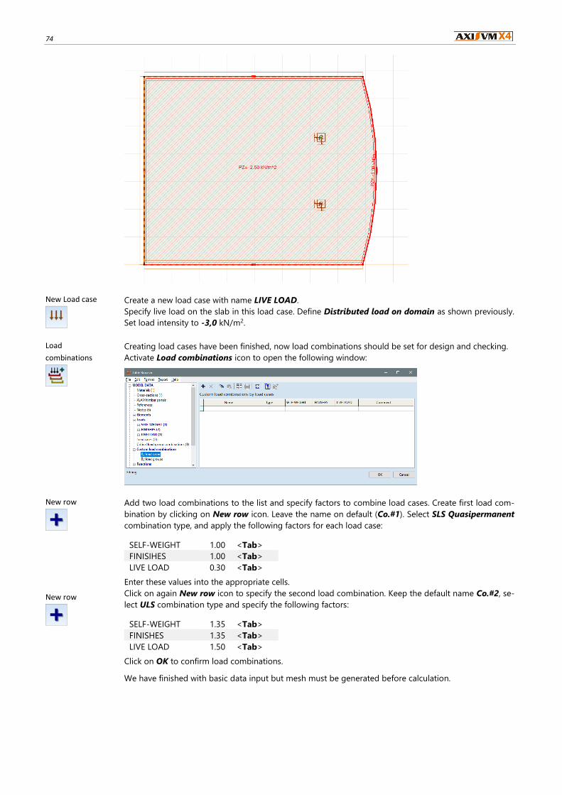
New Load case
Create a new load case with name LIVE LOAD.
Specify live load on the slab in this load case. Define Distributed load on domain as shown previously.
Set load intensity to -3,0 kN/m2.
Load
combinations
Creating load cases have been finished, now load combinations should be set for design and checking.
Activate Load combinations icon to open the following window:
New row
Add two load combinations to the list and specify factors to combine load cases. Create first load com-
bination by clicking on New row icon. Leave the name on default (Co.#1). Select SLS Quasipermanent
combination type, and apply the following factors for each load case:
SELF-WEIGHT 1.00 <Tab>
FINISIHES 1.00 <Tab>
LIVE LOAD 0.30 <Tab>
Enter these values into the appropriate cells.
New row
Click on again New row icon to specify the second load combination. Keep the default name Co.#2, se-
lect ULS combination type and specify the following factors:
Click on OK to confirm load combinations.
SELF-WEIGHT 1.35 <Tab>
FINISHES 1.35 <Tab>
LIVE LOAD 1.50 <Tab>
We have finished with basic data input but mesh must be generated before calculation.
Step by step tutorial 75
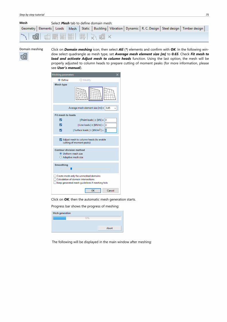
Mesh Select Mesh tab to define domain mesh:
Domain meshing
Click on Domain meshing icon, then select All (*) elements and confirm with OK. In the following win-
dow select quadrangle as mesh type, set Average mesh element size [m] to 0.65. Check Fit mesh to
load and activate Adjust mesh to column heads function. Using the last option, the mesh will be
properly adjusted to column heads to prepare cutting of moment peaks (for more information, please
see User’s manual).
Click on OK, then the automatic mesh generation starts.
Progress bar shows the progress of meshing:
The following will be displayed in the main window after meshing:
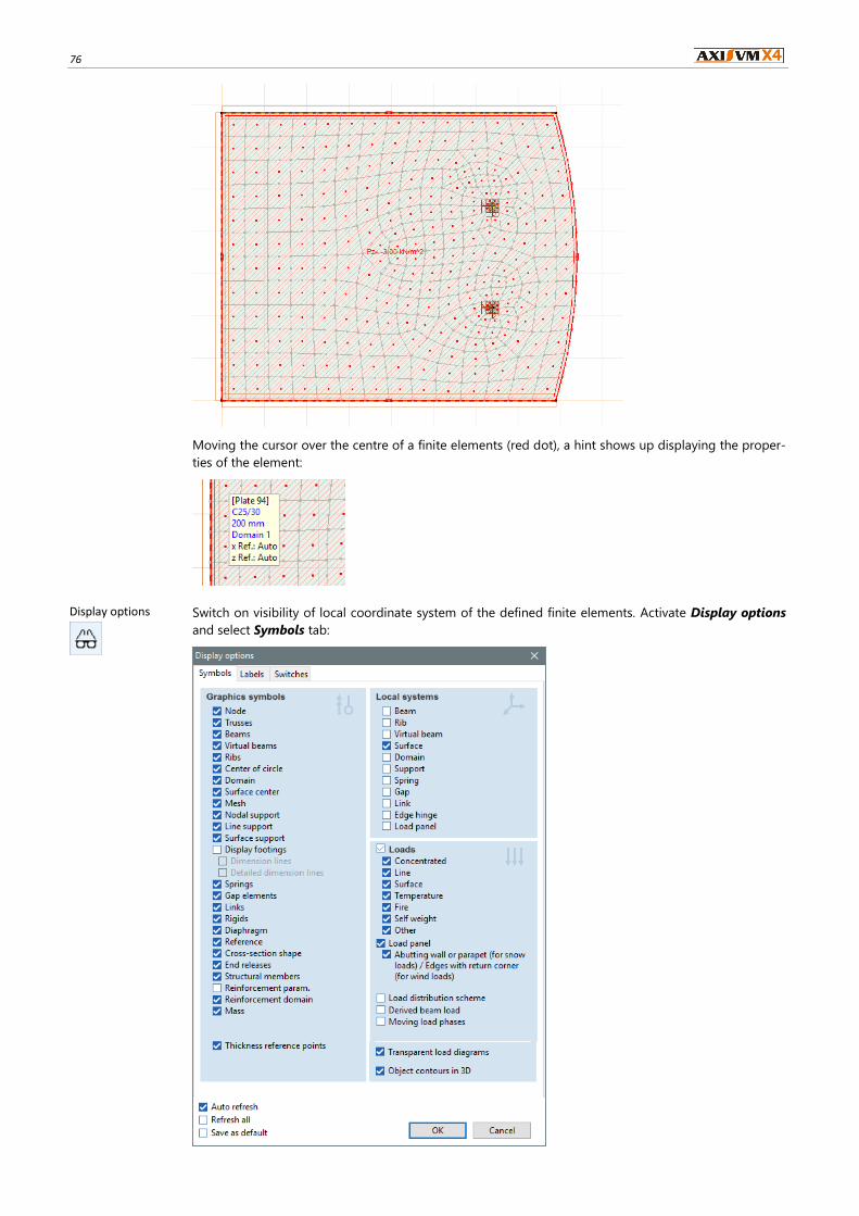
76
Moving the cursor over the centre of a finite elements (red dot), a hint shows up displaying the proper-
ties of the element:
Display options
Switch on visibility of local coordinate system of the defined finite elements. Activate Display options
and select Symbols tab:

Step by step tutorial 77
In Local systems group, check Surface checkbox and close window with OK.
Now, the local system is shown on every finite element: the red line denotes x direction, yellow for y
direction and green for z direction.
Display options
Switch off Local system of Surface elements in Display options window, this will not be necessary
now.
Static Click on Static tab to analyse the model:
Linear static
analysis
Click on Linear static analysis icon to run analysis.
Nodal degrees of freedom
Program checks the model, warns to set nodal degrees of freedom and offers one type in the following
dialog box:
Check Save model with these settings checkbox and degree of freedom settings will be saved. Click
on Yes to accept suggestion (Plane in X-Y plane), then program continues analysis.
The progress bar shows the calculation process:
Click on Statistics to see more information about the analysis.

78
The top progress bar shows progress of the actual task. The progress bar bellow is showing the total
progress. Estimated Memory Requirement shows size of used virtual memory for analysis. If the PC’s
memory size is less than this, error message regarding size of virtual memory will be displayed.
The calculation closes with the next window, then click on OK to close window.
Returning to the main window, the program displays automatically vertical deformations ez [mm] con-
sidering SELF-WEIGHT load case in Isosurfaces 2D display mode.
Select load combination Co.#1 (SLS) to check serviceability limit states (note: this is only the result of
linear analysis):
Deformation values are negative because the positive direction of global Z axis is opposite to the direc-
tion of the specified loads.
Min, max values
To find location of maximum deformation, use Min, max values function. By clicking on icon, shows up
following window:
Step by step tutorial 79
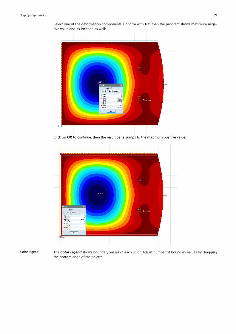
Select one of the deformation components. Confirm with OK, then the program shows maximum nega-
tive value and its location as well:
Click on OK to continue, then the result panel jumps to the maximum positive value:
Color legend The Color legend shows boundary values of each color. Adjust number of boundary values by dragging
the bottom edge of the palette:
80
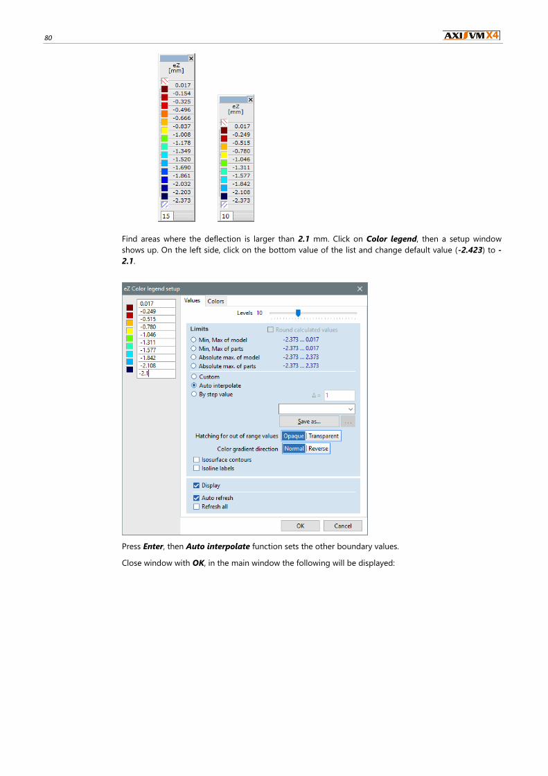
Find areas where the deflection is larger than 2.1 mm. Click on Color legend, then a setup window
shows up. On the left side, click on the bottom value of the list and change default value (-2.423) to -
2.1.
Press Enter, then Auto interpolate function sets the other boundary values.
Close window with OK, in the main window the following will be displayed:
Step by step tutorial 81
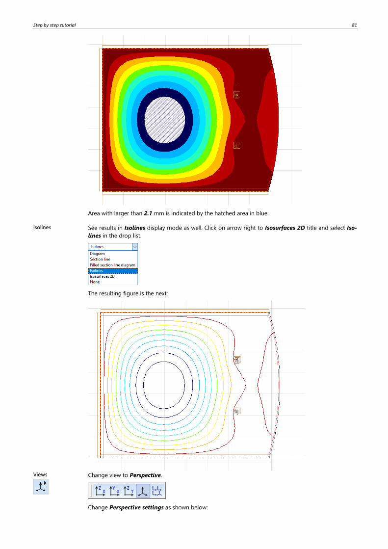
Area with larger than 2.1 mm is indicated by the hatched area in blue.
Isolines See results in Isolines display mode as well. Click on arrow right to Isosurfaces 2D title and select Iso-
lines in the drop list.
The resulting figure is the next:
Views
Change view to Perspective.
Change Perspective settings as shown below:
82
then click on X in the top right corner to close window.
Result display
parameters
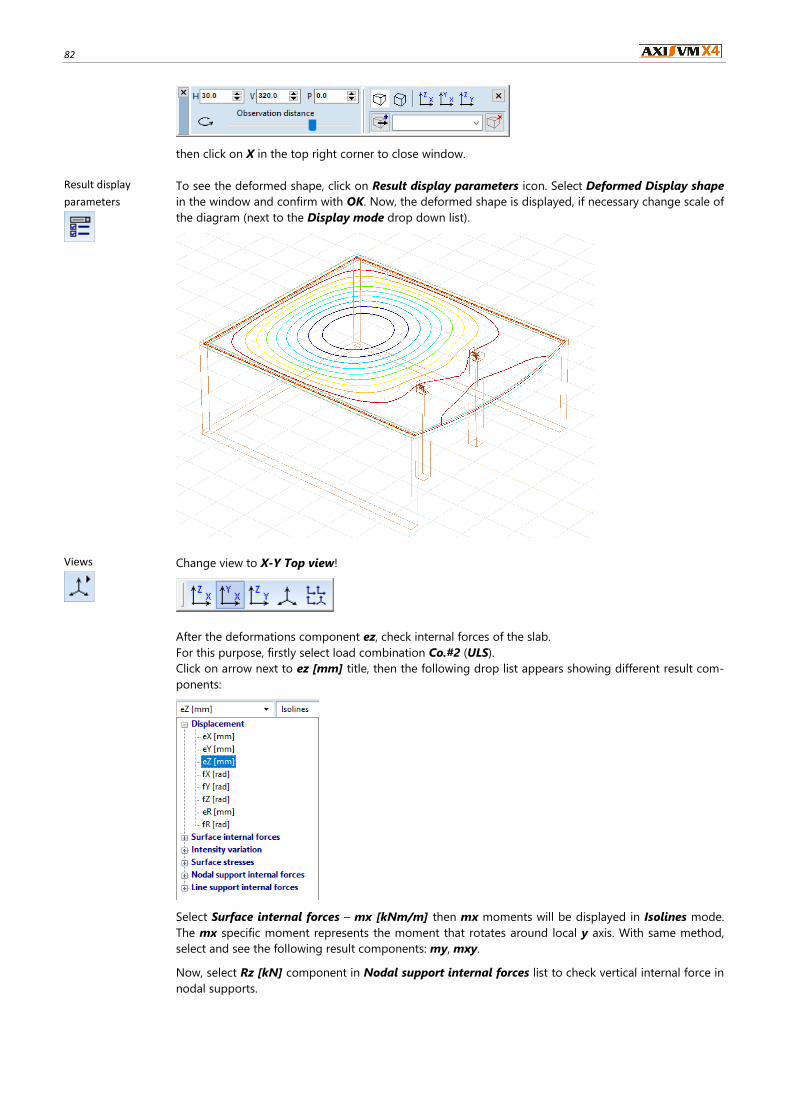
To see the deformed shape, click on Result display parameters icon. Select Deformed Display shape
in the window and confirm with OK. Now, the deformed shape is displayed, if necessary change scale of
the diagram (next to the Display mode drop down list).
Views
Change view to X-Y Top view!
After the deformations component ez, check internal forces of the slab.
For this purpose, firstly select load combination Co.#2 (ULS).
Click on arrow next to ez [mm] title, then the following drop list appears showing different result com-
ponents:
Select Surface internal forces – mx [kNm/m] then mx moments will be displayed in Isolines mode.
The mx specific moment represents the moment that rotates around local y axis. With same method,
select and see the following result components: my, mxy.
Now, select Rz [kN] component in Nodal support internal forces list to check vertical internal force in
nodal supports.
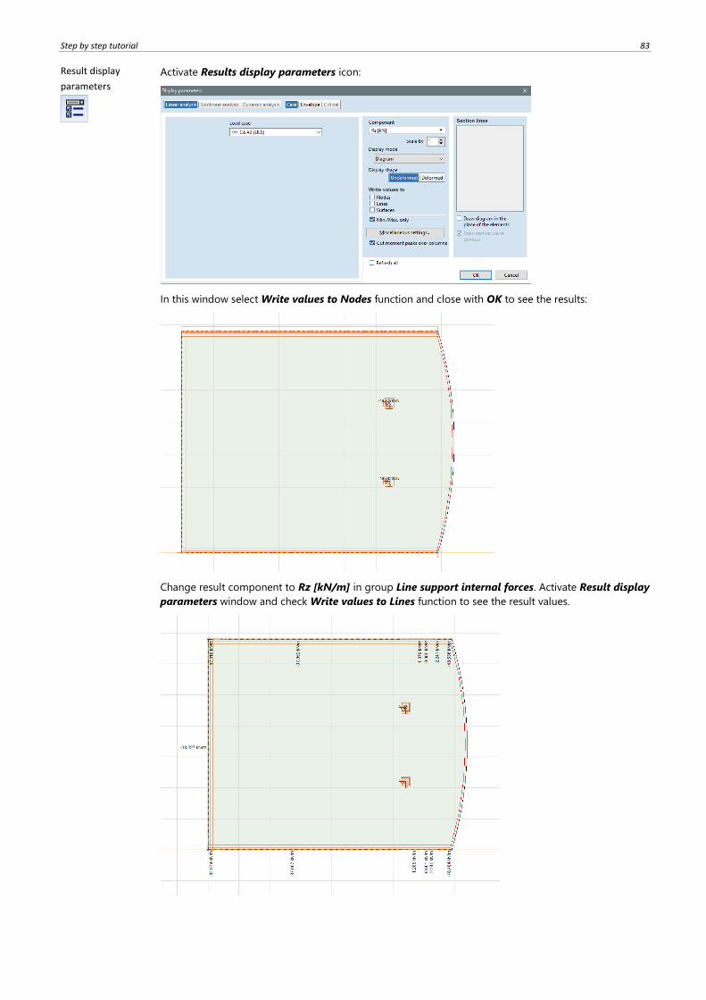
Step by step tutorial 83
Result display
parameters
Activate Results display parameters icon:
In this window select Write values to Nodes function and close with OK to see the results:
Change result component to Rz [kN/m] in group Line support internal forces. Activate Result display
parameters window and check Write values to Lines function to see the result values.
84
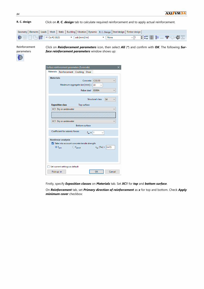
R. C. design Click on R. C. design tab to calculate required reinforcement and to apply actual reinforcement.
Reinforcement
parameters
Click on Reinforcement parameters icon, then select All (*) and confirm with OK. The following Sur-
face reinforcement parameters window shows up:
Firstly, specify Exposition classes on Materials tab. Set XC1 for top and bottom surface.
On Reinforcement tab, set Primary direction of reinforcement as x for top and bottom. Check Apply
minimum cover checkbox:
Step by step tutorial 85
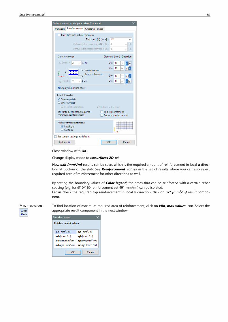
Close window with OK.
Change display mode to Isosurfaces 2D-re!
Now axb [mm2/m] results can be seen, which is the required amount of reinforcement in local x direc-
tion at bottom of the slab. See Reinforcement values in the list of results where you can also select
required area of reinforcement for other directions as well.
By setting the boundary values of Color legend, the areas that can be reinforced with a certain rebar
spacing (e.g. for Ø10/160 reinforcement set 491 mm2/m) can be isolated.
Let us check the required top reinforcement in local x direction, click on axt [mm2/m] result compo-
nent.
Min, max values
To find location of maximum required area of reinforcement, click on Min, max values icon. Select the
appropriate result component in the next window:
86
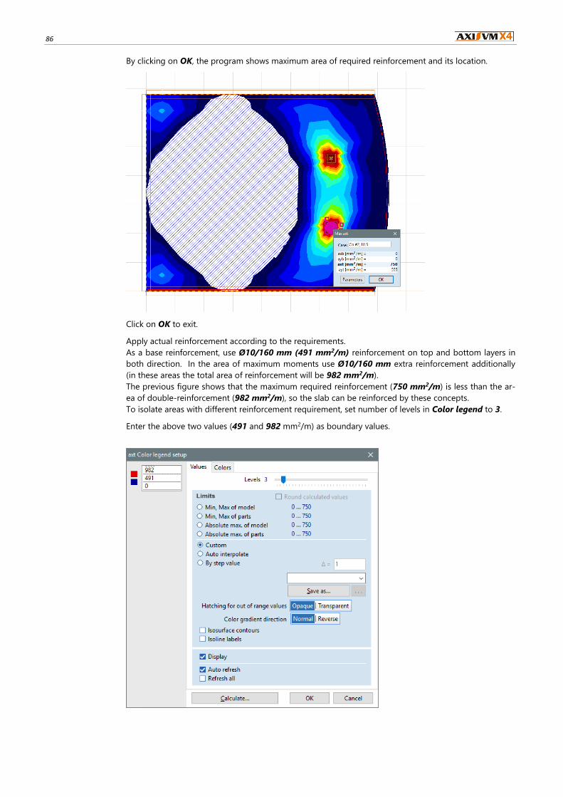
By clicking on OK, the program shows maximum area of required reinforcement and its location.
Click on OK to exit.
Apply actual reinforcement according to the requirements.
As a base reinforcement, use Ø10/160 mm (491 mm2/m) reinforcement on top and bottom layers in
both direction. In the area of maximum moments use Ø10/160 mm extra reinforcement additionally
(in these areas the total area of reinforcement will be 982 mm2/m).
The previous figure shows that the maximum required reinforcement (750 mm2/m) is less than the ar-
ea of double-reinforcement (982 mm2/m), so the slab can be reinforced by these concepts.
To isolate areas with different reinforcement requirement, set number of levels in Color legend to 3.
Enter the above two values (491 and 982 mm2/m) as boundary values.
Step by step tutorial 87
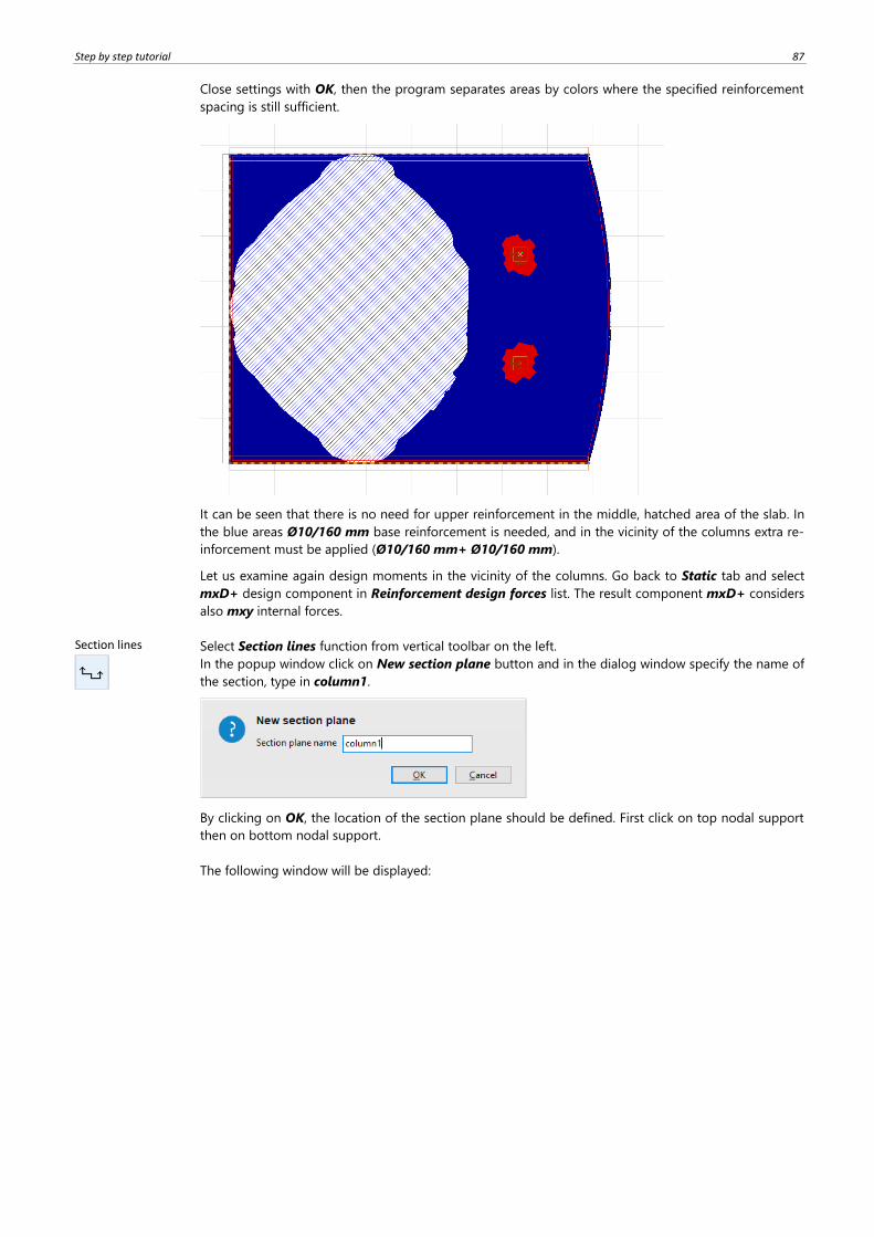
Close settings with OK, then the program separates areas by colors where the specified reinforcement
spacing is still sufficient.
It can be seen that there is no need for upper reinforcement in the middle, hatched area of the slab. In
the blue areas Ø10/160 mm base reinforcement is needed, and in the vicinity of the columns extra re-
inforcement must be applied (Ø10/160 mm+ Ø10/160 mm).
Let us examine again design moments in the vicinity of the columns. Go back to Static tab and select
mxD+ design component in Reinforcement design forces list. The result component mxD+ considers
also mxy internal forces.
Section lines
Select Section lines function from vertical toolbar on the left.
In the popup window click on New section plane button and in the dialog window specify the name of
the section, type in column1.
By clicking on OK, the location of the section plane should be defined. First click on top nodal support
then on bottom nodal support.
The following window will be displayed:
88
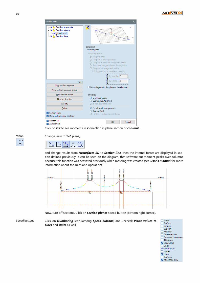
Click on OK to see moments in x direction in plane section of column1.
Views
Change view to Y-Z plane,
and change results from Isosurfaces 2D to Section line, then the internal forces are displayed in sec-
tion defined previously. It can be seen on the diagram, that software cut moment peaks over columns
because this function was activated previously when meshing was created (see User’s manual for more
information about the rules and operation).
Now, turn off sections. Click on Section planes speed button (bottom right corner).
Speed buttons Click on Numbering icon (among Speed buttons) and uncheck Write values to
Lines and Units as well.
Step by step tutorial 89
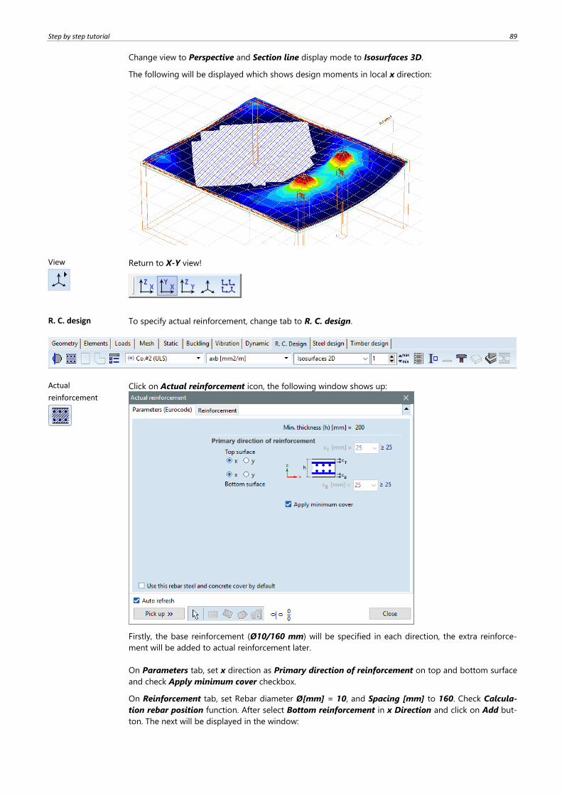
Change view to Perspective and Section line display mode to Isosurfaces 3D.
The following will be displayed which shows design moments in local x direction:
View
Return to X-Y view!
R. C. design To specify actual reinforcement, change tab to R. C. design.
Actual
reinforcement
Click on Actual reinforcement icon, the following window shows up:
Firstly, the base reinforcement (Ø10/160 mm) will be specified in each direction, the extra reinforce-
ment will be added to actual reinforcement later.
On Parameters tab, set x direction as Primary direction of reinforcement on top and bottom surface
and check Apply minimum cover checkbox.
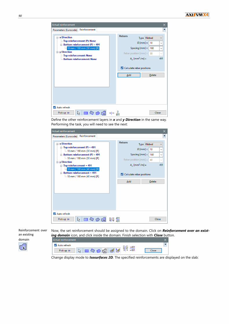
On Reinforcement tab, set Rebar diameter Ø[mm] = 10, and Spacing [mm] to 160. Check Calcula-
tion rebar position function. After select Bottom reinforcement in x Direction and click on Add but-
ton. The next will be displayed in the window:
90
Define the other reinforcement layers in x and y Direction in the same way.
Performing the task, you will need to see the next:
Reinforcement over an existing
domain
Now, the set reinforcement should be assigned to the domain. Click on Reinforcement over an exist-
ing domain icon, and click inside the domain. Finish selection with Close button.
Change display mode to Isosurfaces 2D. The specified reinforcements are displayed on the slab:
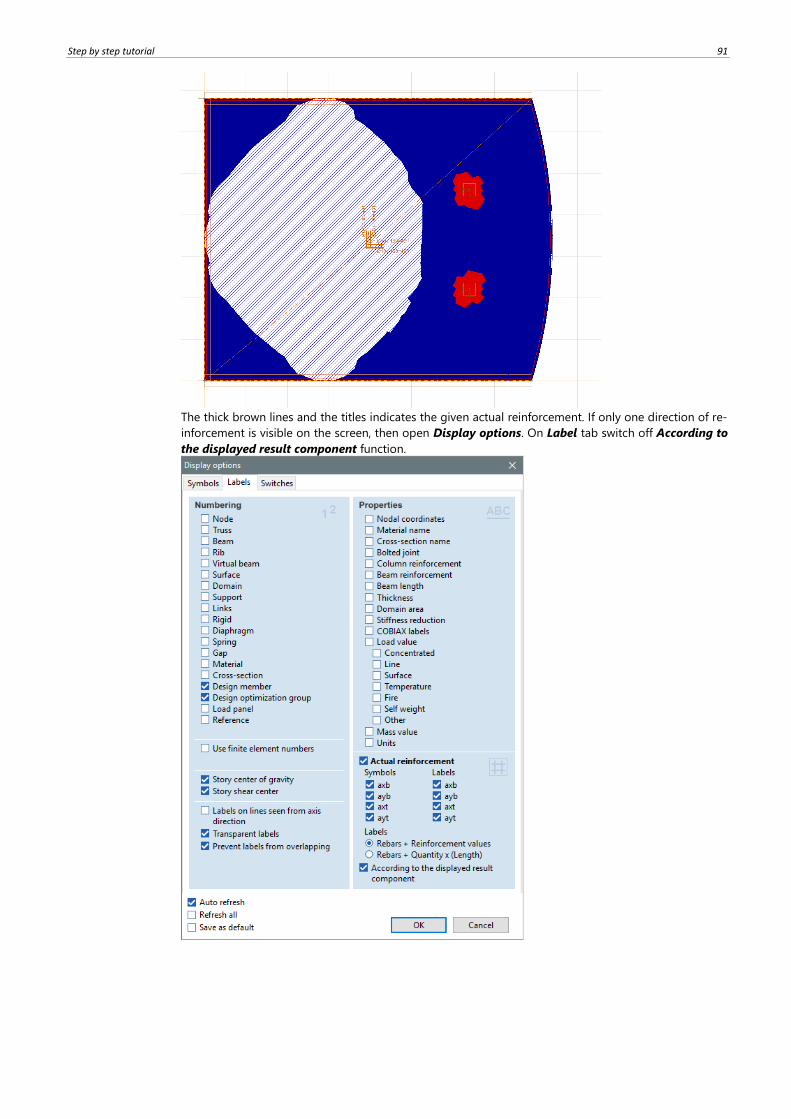
Step by step tutorial 91
The thick brown lines and the titles indicates the given actual reinforcement. If only one direction of re-
inforcement is visible on the screen, then open Display options. On Label tab switch off According to
the displayed result component function.
92
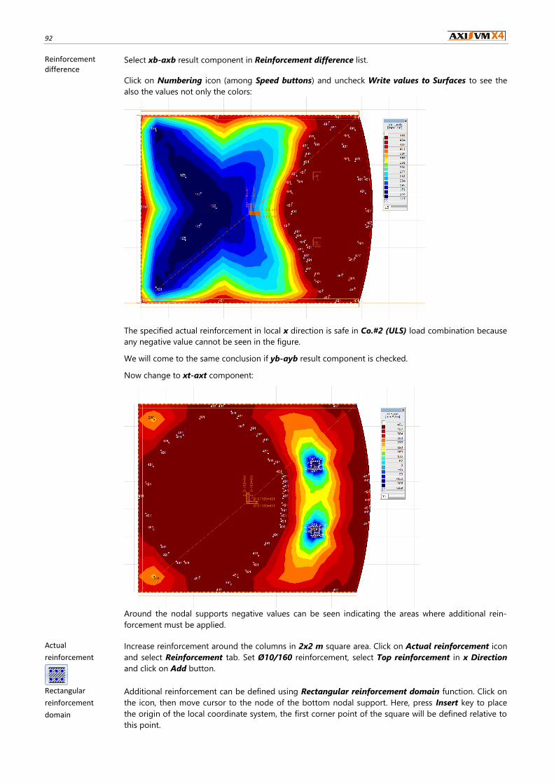
Reinforcement difference
Select xb-axb result component in Reinforcement difference list.
Click on Numbering icon (among Speed buttons) and uncheck Write values to Surfaces to see the
also the values not only the colors:
The specified actual reinforcement in local x direction is safe in Co.#2 (ULS) load combination because
any negative value cannot be seen in the figure.
We will come to the same conclusion if yb-ayb result component is checked.
Now change to xt-axt component:
Around the nodal supports negative values can be seen indicating the areas where additional rein-
forcement must be applied.
Actual
reinforcement
Increase reinforcement around the columns in 2x2 m square area. Click on Actual reinforcement icon
and select Reinforcement tab. Set Ø10/160 reinforcement, select Top reinforcement in x Direction
and click on Add button.
Rectangular
reinforcement
domain
Additional reinforcement can be defined using Rectangular reinforcement domain function. Click on
the icon, then move cursor to the node of the bottom nodal support. Here, press Insert key to place
the origin of the local coordinate system, the first corner point of the square will be defined relative to
this point.

Step by step tutorial 93
Using relative coordinates, enter the following coordinates:
finally press Esc twice to exit.
The following will be the result:
x -1 y -1 z 0 <Enter>
x 2 y 2 z 0 <Enter>
The results of xt-axt component around the bottom lower nodal support are positive, so the actual re-
inforcement is sufficient with the additional reinforcement.
Translate / Copy
Copy this actual reinforcement domain to the upper nodal support. Click on Translate icon:
Then move the cursor over the contour of reinforcement domain and click on it to select. Confirm with
OK to finish selection. In the Translate window select Incremental Method and set N=1:
Close window with OK and define translation vector by clicking on lower and after on upper nodal sup-
port. Performing these steps, we have copied the actual domain reinforcement, the following will be
displayed:
94
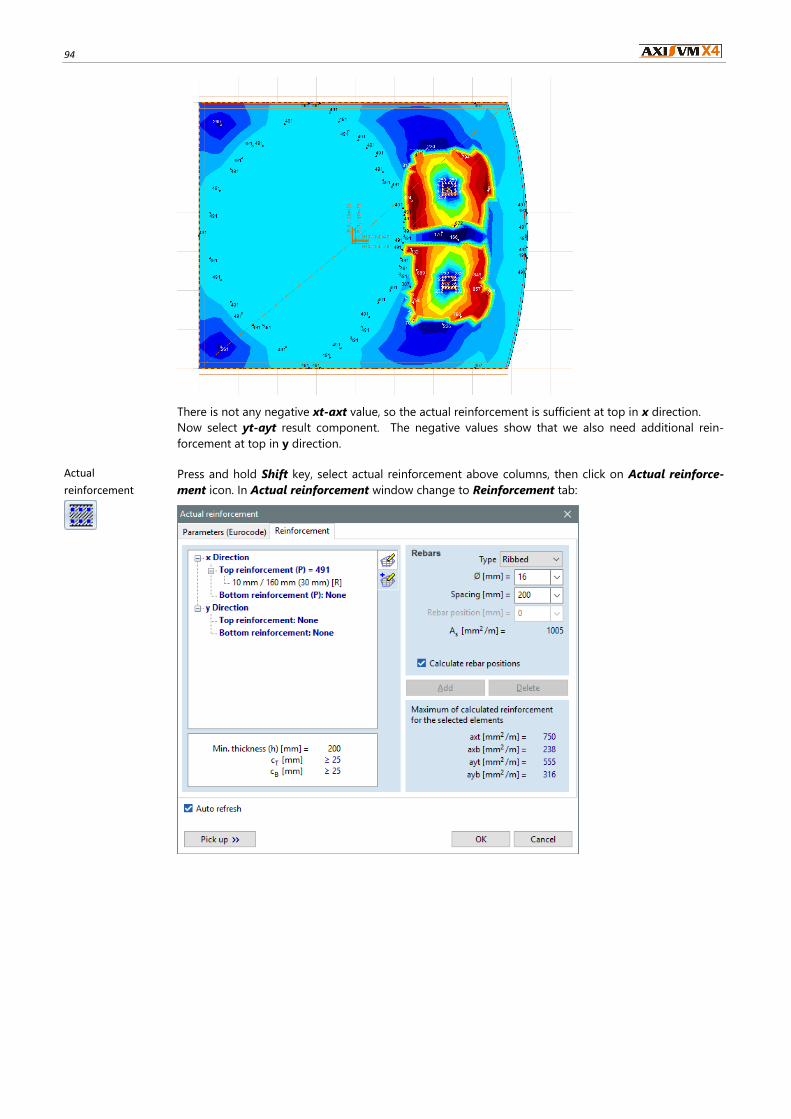
There is not any negative xt-axt value, so the actual reinforcement is sufficient at top in x direction.
Now select yt-ayt result component. The negative values show that we also need additional rein-
forcement at top in y direction.
Actual
reinforcement
Press and hold Shift key, select actual reinforcement above columns, then click on Actual reinforce-
ment icon. In Actual reinforcement window change to Reinforcement tab:
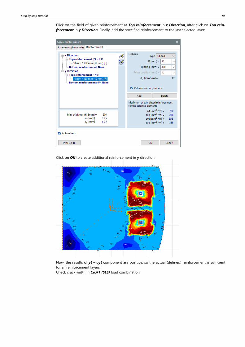
Step by step tutorial 95
Click on the field of given reinforcement at Top reinforcement in x Direction, after click on Top rein-
forcement in y Direction. Finally, add the specified reinforcement to the last selected layer:
Click on OK to create additional reinforcement in y direction.
Now, the results of yt – ayt component are positive, so the actual (defined) reinforcement is sufficient
for all reinforcement layers.
Check crack width in Co.#1 (SLS) load combination.
96
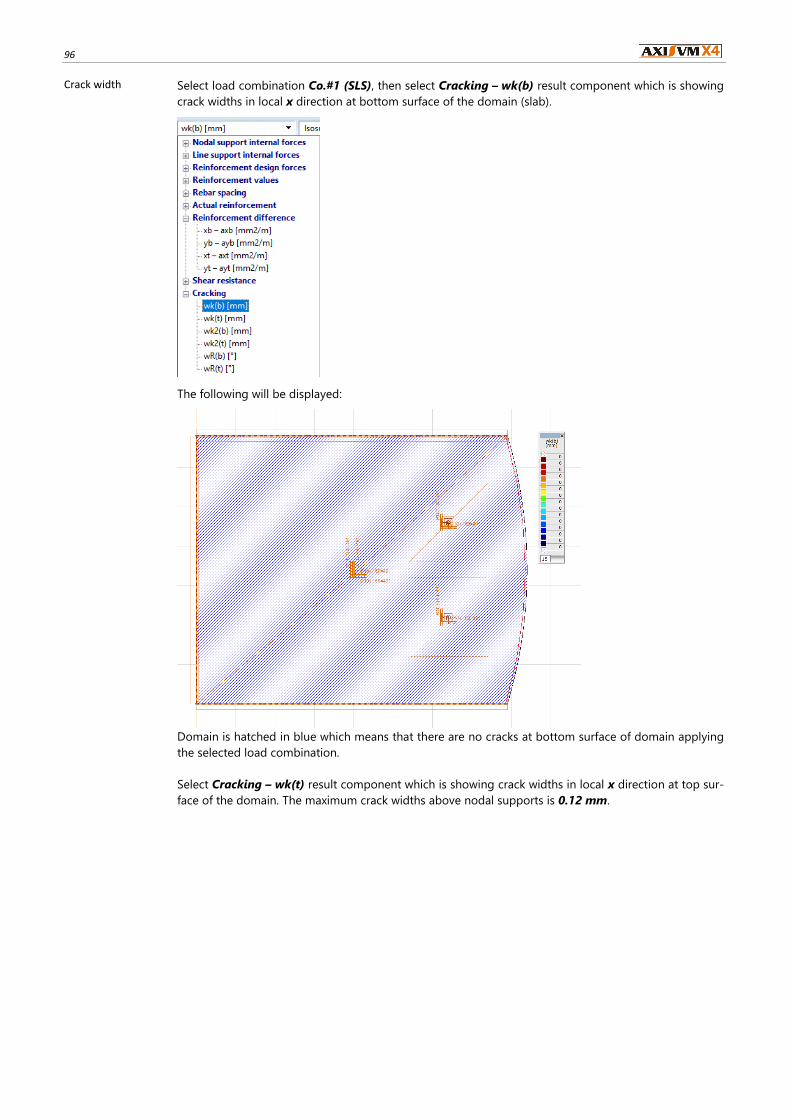
Crack width Select load combination Co.#1 (SLS), then select Cracking – wk(b) result component which is showing
crack widths in local x direction at bottom surface of the domain (slab).
The following will be displayed:
Domain is hatched in blue which means that there are no cracks at bottom surface of domain applying
the selected load combination.
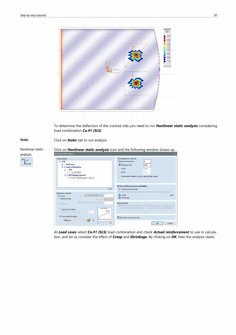
Select Cracking – wk(t) result component which is showing crack widths in local x direction at top sur-
face of the domain. The maximum crack widths above nodal supports is 0.12 mm.
Step by step tutorial 97
To determine the deflection of the cracked slab you need to run Nonlinear static analysis considering
load combination Co.#1 (SLS).
Static Click on Static tab to run analysis.
Nonlinear static
analysis
Click on Nonlinear static analysis icon and the following window shows up:
At Load cases select Co.#1 (SLS) load combination and check Actual reinforcement to use in calcula-
tion, and let us consider the effect of Creep and Shrinkage. By clicking on OK, then the analysis starts:
98
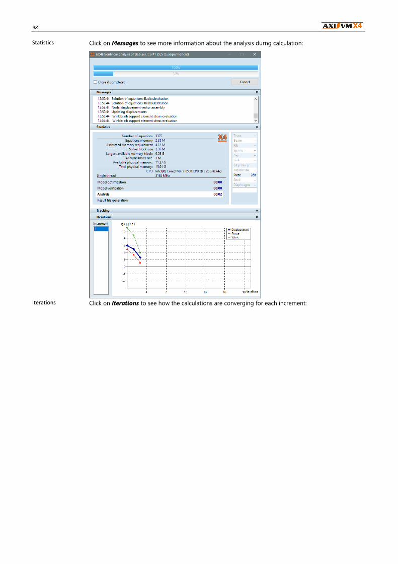
Statistics Click on Messages to see more information about the analysis durng calculation:
Iterations Click on Iterations to see how the calculations are converging for each increment:
Step by step tutorial 99
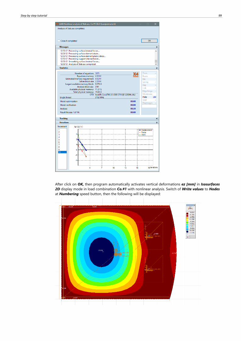
After click on OK, then program automatically activates vertical deformations ez [mm] in Isosurfaces
2D display mode in load combination Co.#1 with nonlinear analysis. Switch of Write values to Nodes
at Numbering speed button, then the following will be displayed:
100
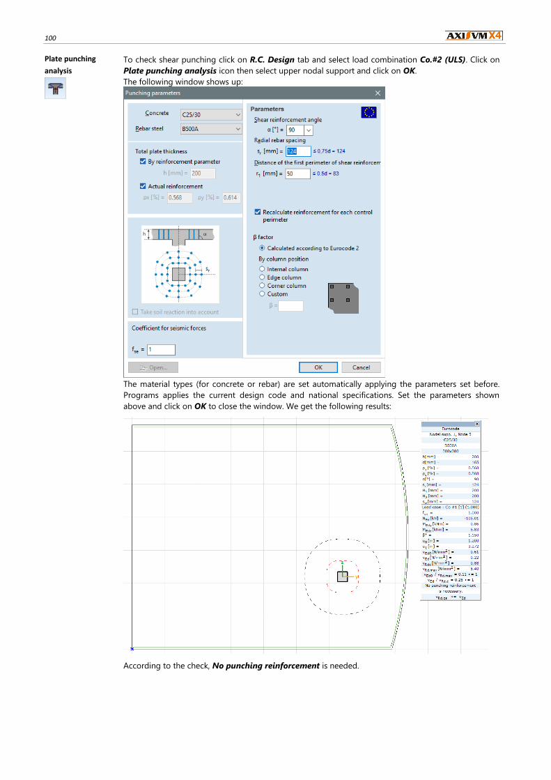
Plate punching
analysis
To check shear punching click on R.C. Design tab and select load combination Co.#2 (ULS). Click on
Plate punching analysis icon then select upper nodal support and click on OK.
The following window shows up:
The material types (for concrete or rebar) are set automatically applying the parameters set before.
Programs applies the current design code and national specifications. Set the parameters shown
above and click on OK to close the window. We get the following results:
According to the check, No punching reinforcement is needed.
Step by step tutorial 101
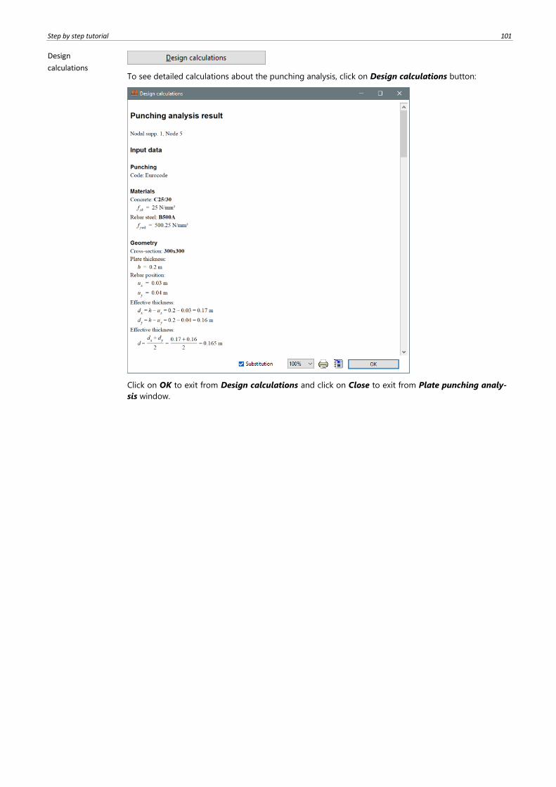
Design
calculations
To see detailed calculations about the punching analysis, click on Design calculations button:
Click on OK to exit from Design calculations and click on Close to exit from Plate punching analy-
sis window.

102
Intentionally blank page
Step by step tutorial 103
4. MEMBRANE MODEL
4.1. Geometry definition using parametric mesh
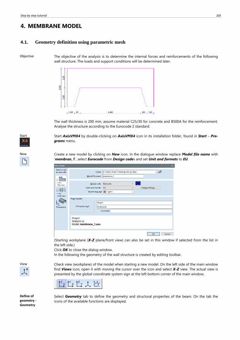
Objective The objective of the analysis is to determine the internal forces and reinforcements of the following
wall structure. The loads and support conditions will be determined later.
The wall thickness is 200 mm, assume material C25/30 for concrete and B500A for the reinforcement.
Analyse the structure according to the Eurocode 2 standard.
Start
Start AxisVMX4 by double-clicking on AxisVMX4 icon in its installation folder, found in Start – Pro-
grams menu.
New
Create a new model by clicking on New icon. In the dialogue window replace Model file name with
‘membran_1’, select Eurocode from Design codes and set Unit and formats to EU.
(Starting workplane (X-Z plane/front view) can also be set in this window if selected from the list in
the left side.)
Click OK to close the dialog window.
In the following the geometry of the wall structure is created by editing toolbar.
View
Check view (workplane) of the model when starting a new model. On the left side of the main window
find Views icon, open it with moving the cursor over the icon and select X-Z view. The actual view is
presented by the global coordinate system sign at the left bottom corner of the main window.
Define of geometry - Geometry
Select Geometry tab to define the geometry and structural properties of the beam. On the tab the
icons of the available functions are displayed.
104
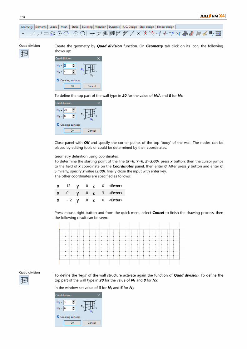
Quad division
Create the geometry by Quad division function. On Geometry tab click on its icon, the following
shows up:
To define the top part of the wall type in 20 for the value of N1A and 8 for N2:
Close panel with OK and specify the corner points of the top ‘body’ of the wall. The nodes can be
placed by editing tools or could be determined by their coordinates.
Geometry definition using coordinates:
To determine the starting point of the line (X=0, Y=0, Z=3.00), press x button, then the cursor jumps
to the field of x coordinate on the Coordinates panel, then enter 0. After press y button and enter 0.
Similarly, specify z value (3.00), finally close the input with enter key.
The other coordinates are specified as follows:
Press mouse right button and from the quick menu select Cancel to finish the drawing process, then
the following result can be seen:
x 12 y 0 z 0 <Enter>
x 0 y 0 z 3 <Enter>
x -12 y 0 z 0 <Enter>
Quad division
To define the ‘legs’ of the wall structure activate again the function of Quad division. To define the
top part of the wall type in 20 for the value of N1 and 8 for N2:
In the window set value of 3 for N1 and 6 for N2:
Step by step tutorial 105
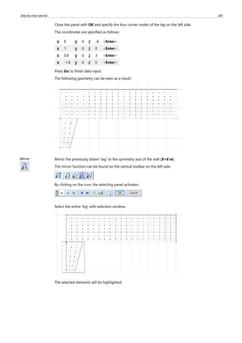
Close the panel with OK and specify the four corner nodes of the leg on the left side.
The coordinates are specified as follows:
Press Esc to finish data input.
x 0 y 0 z -6 <Enter>
x 1 y 0 z 0 <Enter>
x 0.8 y 0 z 3 <Enter>
x -1.8 y 0 z 0 <Enter>
The following geometry can be seen as a result:
Mirror
Mirror the previously drawn ‘leg’ to the symmetry axis of the wall (X=6 m).
The mirror function can be found on the vertical toolbar on the left side.
By clicking on the icon, the selecting panel activates:
Select the entire ‘leg’ with selection window.
The selected elements will be highlighted:

106
Finish the selection with OK and the following dialogue panel will be displayed:
Select Multiple Mirror type and set None for Nodes to connect.
After clicking on OK, the mirror plane should be specified. First select any point on the symmetric
plane of the wall, then select any point in the vertical direction above or below that point.
As a result of mirroring the following can be seen:
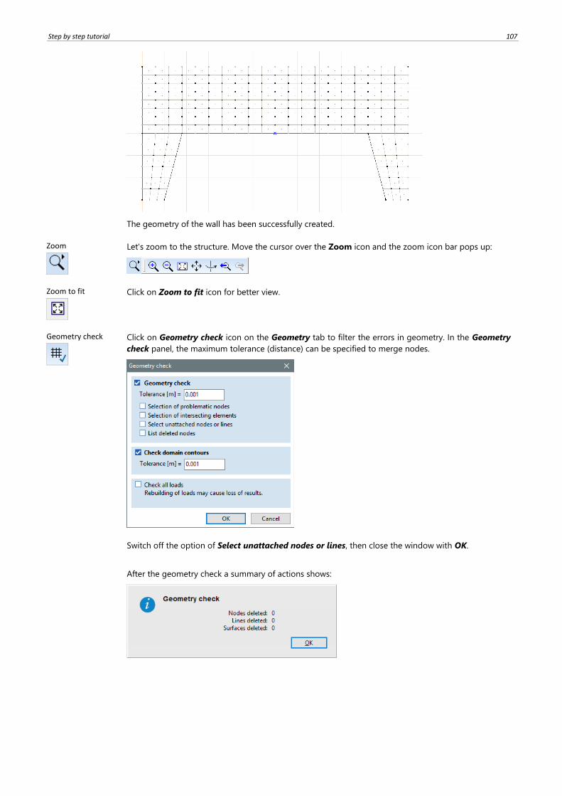
Step by step tutorial 107
The geometry of the wall has been successfully created.
Zoom
Let's zoom to the structure. Move the cursor over the Zoom icon and the zoom icon bar pops up:
Zoom to fit
Click on Zoom to fit icon for better view.
Geometry check
Click on Geometry check icon on the Geometry tab to filter the errors in geometry. In the Geometry
check panel, the maximum tolerance (distance) can be specified to merge nodes.
Switch off the option of Select unattached nodes or lines, then close the window with OK.
After the geometry check a summary of actions shows:
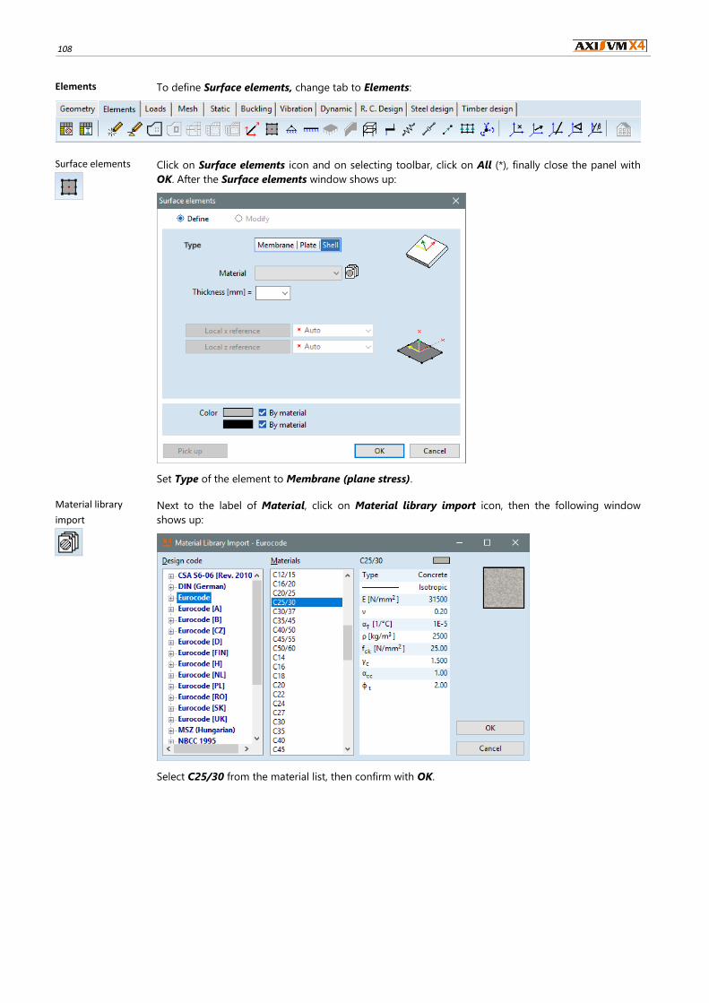
108
Elements To define Surface elements, change tab to Elements:
Surface elements
Click on Surface elements icon and on selecting toolbar, click on All (*), finally close the panel with
OK. After the Surface elements window shows up:
Set Type of the element to Membrane (plane stress).
Material library
import
Next to the label of Material, click on Material library import icon, then the following window
shows up:
Select C25/30 from the material list, then confirm with OK.
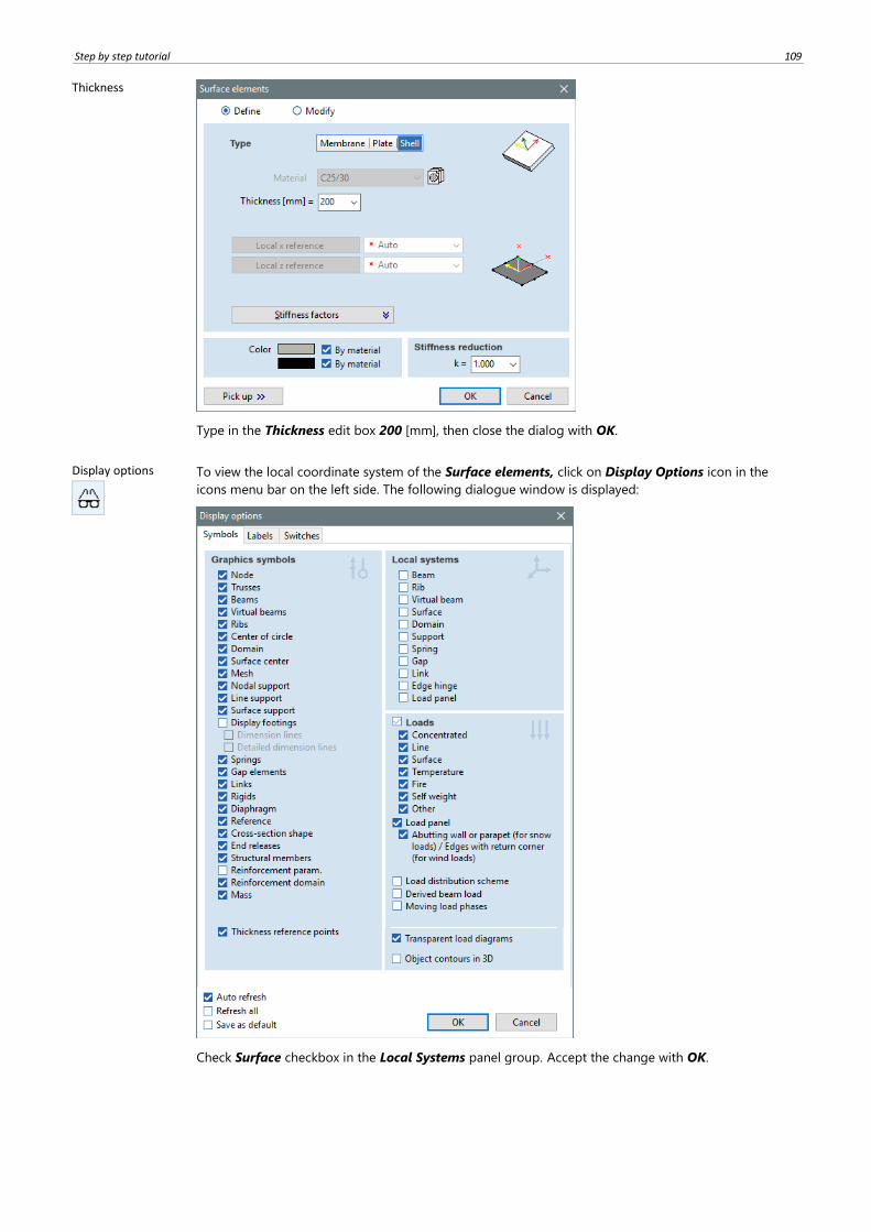
Step by step tutorial 109
Thickness
Type in the Thickness edit box 200 [mm], then close the dialog with OK.
Display options
To view the local coordinate system of the Surface elements, click on Display Options icon in the
icons menu bar on the left side. The following dialogue window is displayed:
Check Surface checkbox in the Local Systems panel group. Accept the change with OK.
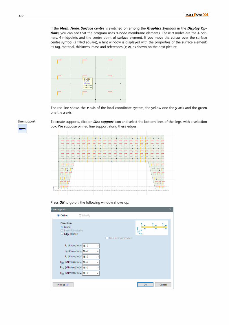
110
If the Mesh, Node, Surface centre is switched on among the Graphics Symbols in the Display Op-
tions, you can see that the program uses 9-node membrane elements. These 9 nodes are the 4 cor-
ners, 4 midpoints and the centre point of surface element. If you move the cursor over the surface
centre symbol (a filled square), a hint window is displayed with the properties of the surface element:
its tag, material, thickness, mass and references (x, z), as shown on the next picture:
The red line shows the x axis of the local coordinate system, the yellow one the y axis and the green
one the z axis.
Line support
To create supports, click on Line support icon and select the bottom lines of the ‘legs’ with a selection
box. We suppose pinned line support along these edges.
Press OK to go on, the following window shows up:
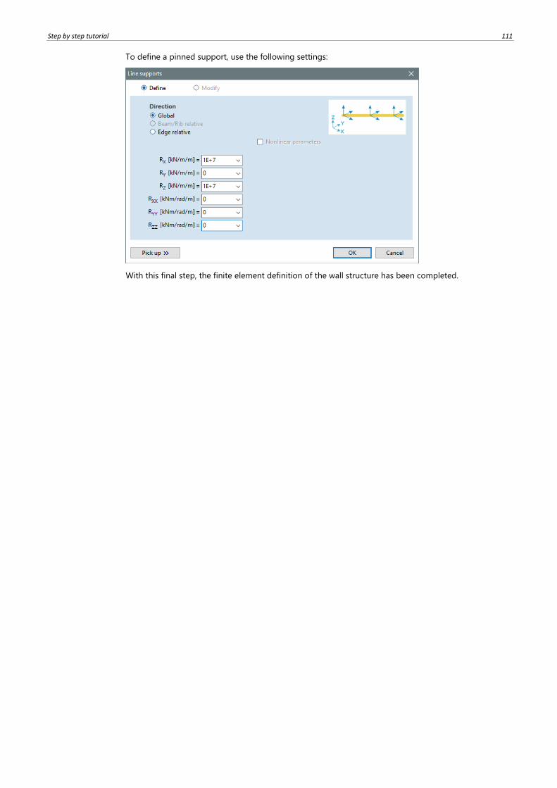
Step by step tutorial 111
To define a pinned support, use the following settings:
With this final step, the finite element definition of the wall structure has been completed.
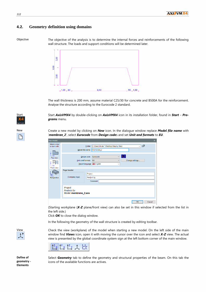
112
4.2. Geometry definition using domains
Objective The objective of the analysis is to determine the internal forces and reinforcements of the following
wall structure. The loads and support conditions will be determined later.
The wall thickness is 200 mm, assume material C25/30 for concrete and B500A for the reinforcement.
Analyse the structure according to the Eurocode 2 standard.
Start
Start AxisVMX4 by double-clicking on AxisVMX4 icon in its installation folder, found in Start – Pro-
grams menu.
New
Create a new model by clicking on New icon. In the dialogue window replace Model file name with
‘membran_2’, select Eurocode from Design codes and set Unit and formats to EU.
(Starting workplane (X-Z plane/front view) can also be set in this window if selected from the list in
the left side.)
Click OK to close the dialog window.
In the following the geometry of the wall structure is created by editing toolbar.
View
Check the view (workplane) of the model when starting a new model. On the left side of the main
window find Views icon, open it with moving the cursor over the icon and select X-Z view. The actual
view is presented by the global coordinate system sign at the left bottom corner of the main window.
Define of geometry - Elements
Select Geometry tab to define the geometry and structural properties of the beam. On this tab the
icons of the available functions are actives.

Step by step tutorial 113
Draw objects
directly
By clicking on Draw objects directly icon brings up the following window:
Domain
Click on Domain icon (the second one on the right among the top row icons). Choose it even if this is
the active icon because of the sequences of steps. The following dialogue panel shows after clicking:
Material library import
The following, Cross-section editor window shows after clicking.
Select C25/30 from the Materials list, then confirm with OK.
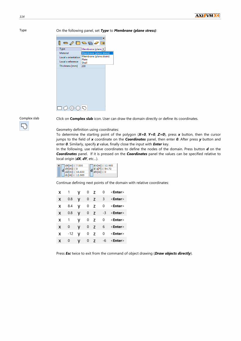
114
Type On the following panel, set Type to Membrane (plane stress):
Complex slab
Click on Complex slab icon. User can draw the domain directly or define its coordinates.
Geometry definition using coordinates:
To determine the starting point of the polygon (X=0, Y=0, Z=0), press x button, then the cursor
jumps to the field of x coordinate on the Coordinates panel, then enter 0. After press y button and
enter 0. Similarly, specify z value, finally close the input with Enter key.
In the following, use relative coordinates to define the nodes of the domain. Press button d on the
Coordinates panel. If it is pressed on the Coordinates panel the values can be specified relative to
local origin (dX, dY, etc…).
Continue defining next points of the domain with relative coordinates:
Press Esc twice to exit from the command of object drawing (Draw objects directly).
x 1 y 0 z 0 <Enter>
x 0.8 y 0 z 3 <Enter>
x 8.4 y 0 z 0 <Enter>
x 0.8 y 0 z -3 <Enter>
x 1 y 0 z 0 <Enter>
x 0 y 0 z 6 <Enter>
x -12 y 0 z 0 <Enter>
x 0 y 0 z -6 <Enter>
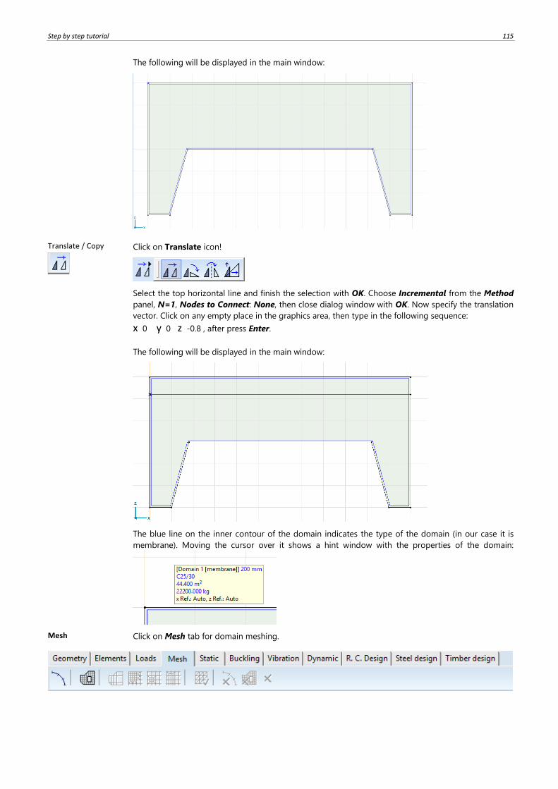
Step by step tutorial 115
The following will be displayed in the main window:
Translate / Copy
Click on Translate icon!
Select the top horizontal line and finish the selection with OK. Choose Incremental from the Method
panel, N=1, Nodes to Connect: None, then close dialog window with OK. Now specify the translation
vector. Click on any empty place in the graphics area, then type in the following sequence:
x 0 y 0 z -0.8 , after press Enter.
The following will be displayed in the main window:
The blue line on the inner contour of the domain indicates the type of the domain (in our case it is
membrane). Moving the cursor over it shows a hint window with the properties of the domain:
Mesh Click on Mesh tab for domain meshing.
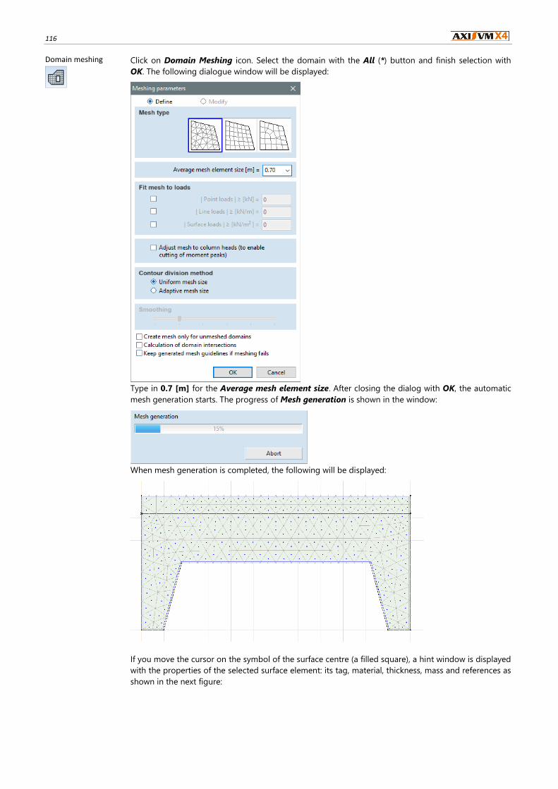
116
Domain meshing
Click on Domain Meshing icon. Select the domain with the All (*) button and finish selection with
OK. The following dialogue window will be displayed:
Type in 0.7 [m] for the Average mesh element size. After closing the dialog with OK, the automatic
mesh generation starts. The progress of Mesh generation is shown in the window:
When mesh generation is completed, the following will be displayed:
If you move the cursor on the symbol of the surface centre (a filled square), a hint window is displayed
with the properties of the selected surface element: its tag, material, thickness, mass and references as
shown in the next figure:
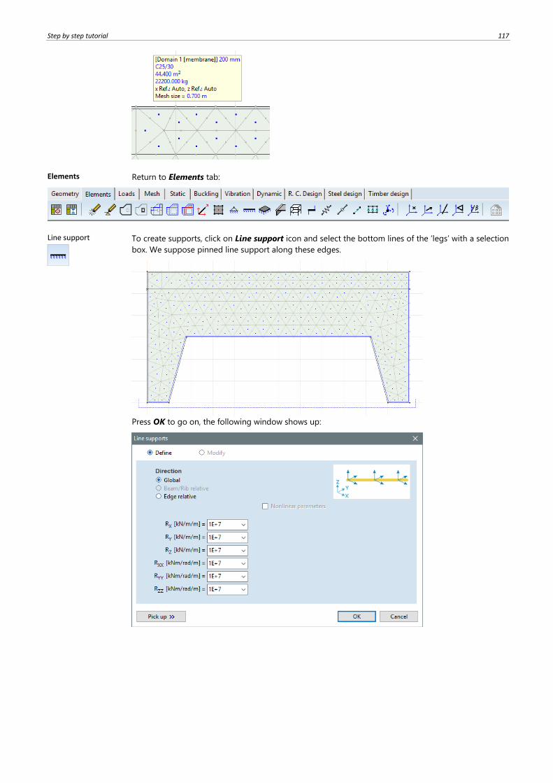
Step by step tutorial 117
Elements Return to Elements tab:
Line support
To create supports, click on Line support icon and select the bottom lines of the ‘legs’ with a selection
box. We suppose pinned line support along these edges.
Press OK to go on, the following window shows up:

118
To define a pinned support, use the following settings:
Close window with OK, the following result can be seen:
With this final step, the finite element definition of the wall structure has been completed. In the fol-
lowing, we proceed the analysis with this model (Geometry definition using domains).
Loads The next step is to specify the loads on the wall structure. Click on Loads tab:

Step by step tutorial 119
Surface edge loads
Assume a 50 kN/m vertical distributed load. Click on Surface Edge Load icon, then select the second
line from top (created with the translate command before):
Finish the selection with OK and type in py [kN/m] to 50:
Press OK and the load is applied.
The following result is displayed:
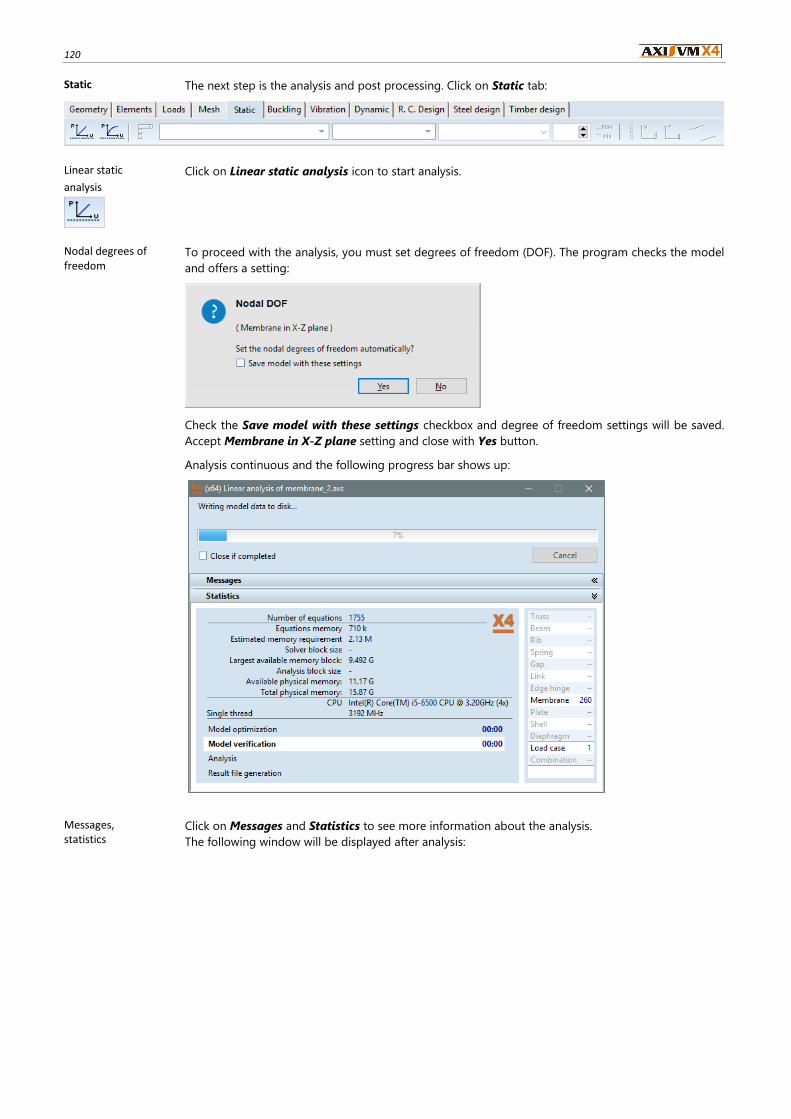
120
Static The next step is the analysis and post processing. Click on Static tab:
Linear static
analysis
Click on Linear static analysis icon to start analysis.
Nodal degrees of freedom
To proceed with the analysis, you must set degrees of freedom (DOF). The program checks the model
and offers a setting:
Check the Save model with these settings checkbox and degree of freedom settings will be saved.
Accept Membrane in X-Z plane setting and close with Yes button.
Analysis continuous and the following progress bar shows up:
Messages, statistics
Click on Messages and Statistics to see more information about the analysis.
The following window will be displayed after analysis:
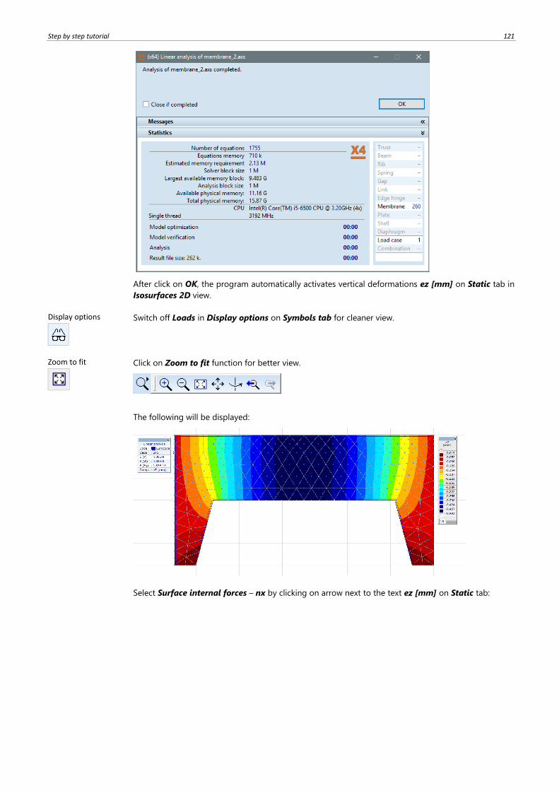
Step by step tutorial 121
After click on OK, the program automatically activates vertical deformations ez [mm] on Static tab in
Isosurfaces 2D view.
Display options
Switch off Loads in Display options on Symbols tab for cleaner view.
Zoom to fit
Click on Zoom to fit function for better view.
The following will be displayed:
Select Surface internal forces – nx by clicking on arrow next to the text ez [mm] on Static tab:

122
The nx diagram shows the membrane force in local x direction.
Min, max values
To find location of minimum and maximum values use Min, Max values function. By clicking on its
icon shows following window:
Select one of the Surface force components. Confirm with OK, and the program shows the negative
maximum value and its location as well.
After click on OK, then the maximum positive value will be showed and its location will be marked.
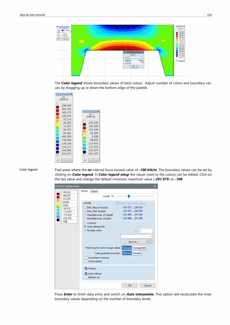
Step by step tutorial 123
The Color legend shows boundary values of each colour. Adjust number of colors and boundary val-
ues by dragging up or down the bottom edge of the palette.
Color legend Find areas where the nx internal force exceed value of -100 kN/m. The boundary values can be set by
clicking on Color legend. In Color legend setup the values (next to the colors) can be edited. Click on
the last value and change the default minimum maximum value (-291.975) to -100:
Press Enter to finish data entry and switch on Auto interpolate. This option will recalculate the inner
boundary values depending on the number of boundary levels.
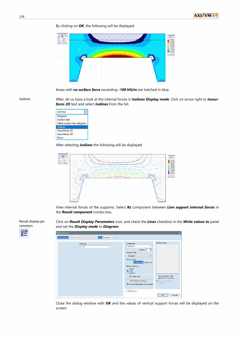
124
By clicking on OK, the following will be displayed:
Areas with nx surface force exceeding -100 kN/m are hatched in blue.
Isolines After, let us have a look at the internal forces in Isolines Display mode. Click on arrow right to Isosur-
faces 2D text and select Isolines from the list.
After selecting Isolines the following will be displayed:
View internal forces of the supports. Select Rz component between Line support internal forces in
the Result component combo box.
Result display pa-rameters
Click on Result Display Parameters icon, and check the Lines checkbox in the Write values to panel
and set the Display mode to Diagram:
Close the dialog window with OK and the values of vertical support forces will be displayed on the
screen:

Step by step tutorial 125
R. C. design
The next step is to calculate the required reinforcement of the wall structure. Click on R. C. design tab:
Reinforcement
parameters
Click on Reinforcement Parameters icon, and select all surface elements with All (*) button. Com-
plete selection with OK, and set the followings on Materials tab:
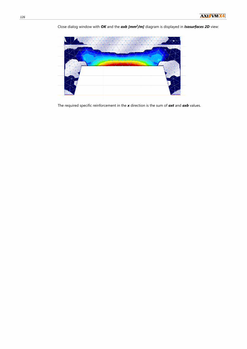
126
Close dialog window with OK and the axb [mm2/m] diagram is displayed in Isosurfaces 2D view:
The required specific reinforcement in the x direction is the sum of axt and axb values.

Step by step tutorial 127
5. SHELL MODEL
Objective Determine the specific internal forces and the amount of reinforcement for the water reservoir shown
below.
The thickness of the walls and the bottom slab is 250 mmm, the cross section of the ribs on the upper
edges is 300x600 mm. The reservoir is made of concrete C25/30, the type of rebar is B500B. Use Euro-
code 2 for design.
Start
Start AxisVMX4 by double-clicking on AxisVMX4 icon in its installation folder, found in Start – Pro-
grams menu.
New
Create a new model by clicking on New icon. In the dialogue window replace Model file name with
‘reservoir’, select Eurocode from Design codes and set Unit and formats to EU.
Options Change settings for grid and cursor step. Click Settings/ Options/ Grid & cursor and set the followings
in the window:

128
Replace each value under Cursor step to 0.2.
,
With these settings, the mouse cursor moves in 0.2 m steps (geometric imperfection or editing error
can be avoided while drawing the model).
Now, create the geometry using enhanced editing functions.
Define of geometry – Elements
Select Elements tab to bring up Elements toolbar.
Draw objects
directly
By clicking on Draw objects directly icon shows following window:
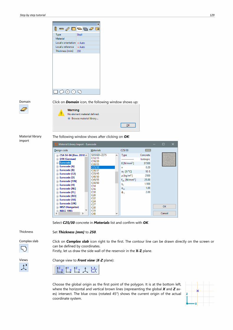
Step by step tutorial 129
Domain
Click on Domain icon, the following window shows up:
Material library import
The following window shows after clicking on OK:
Select C25/30 concrete in Materials list and confirm with OK.
Thickness Set Thickness [mm] to 250.
Complex slab
Click on Complex slab icon right to the first. The contour line can be drawn directly on the screen or
can be defined by coordinates.
Firstly, let us draw the side wall of the reservoir in the X-Z plane.
Views
Change view to Front view (X-Z plane):
Choose the global origin as the first point of the polygon. It is at the bottom left,
where the horizontal and vertical brown lines (representing the global X and Z ax-
es) intersect. The blue cross (rotated 45°) shows the current origin of the actual
coordinate system.
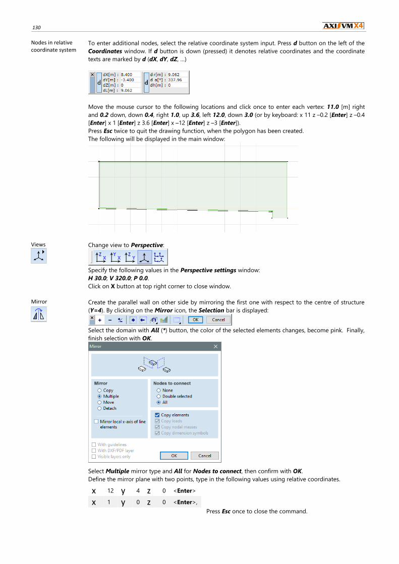
130
Nodes in relative coordinate system
To enter additional nodes, select the relative coordinate system input. Press d button on the left of the
Coordinates window. If d button is down (pressed) it denotes relative coordinates and the coordinate
texts are marked by d (dX, dY, dZ, …)
Move the mouse cursor to the following locations and click once to enter each vertex: 11.0 [m] right
and 0.2 down, down 0.4, right 1.0, up 3.6, left 12.0, down 3.0 (or by keyboard: x 11 z –0.2 [Enter] z –0.4
[Enter] x 1 [Enter] z 3.6 [Enter] x –12 [Enter] z –3 [Enter]).
Press Esc twice to quit the drawing function, when the polygon has been created.
The following will be displayed in the main window:
Views
Change view to Perspective:
Specify the following values in the Perspective settings window:
H 30.0; V 320.0; P 0.0.
Click on X button at top right corner to close window.
Mirror
Create the parallel wall on other side by mirroring the first one with respect to the centre of structure
(Y=4). By clicking on the Mirror icon, the Selection bar is displayed:
Select the domain with All (*) button, the color of the selected elements changes, become pink. Finally,
finish selection with OK.
Select Multiple mirror type and All for Nodes to connect, then confirm with OK.
Define the mirror plane with two points, type in the following values using relative coordinates.
Press Esc once to close the command.
x 12 y 4 z 0 <Enter>
x 1 y 0 z 0 <Enter>,
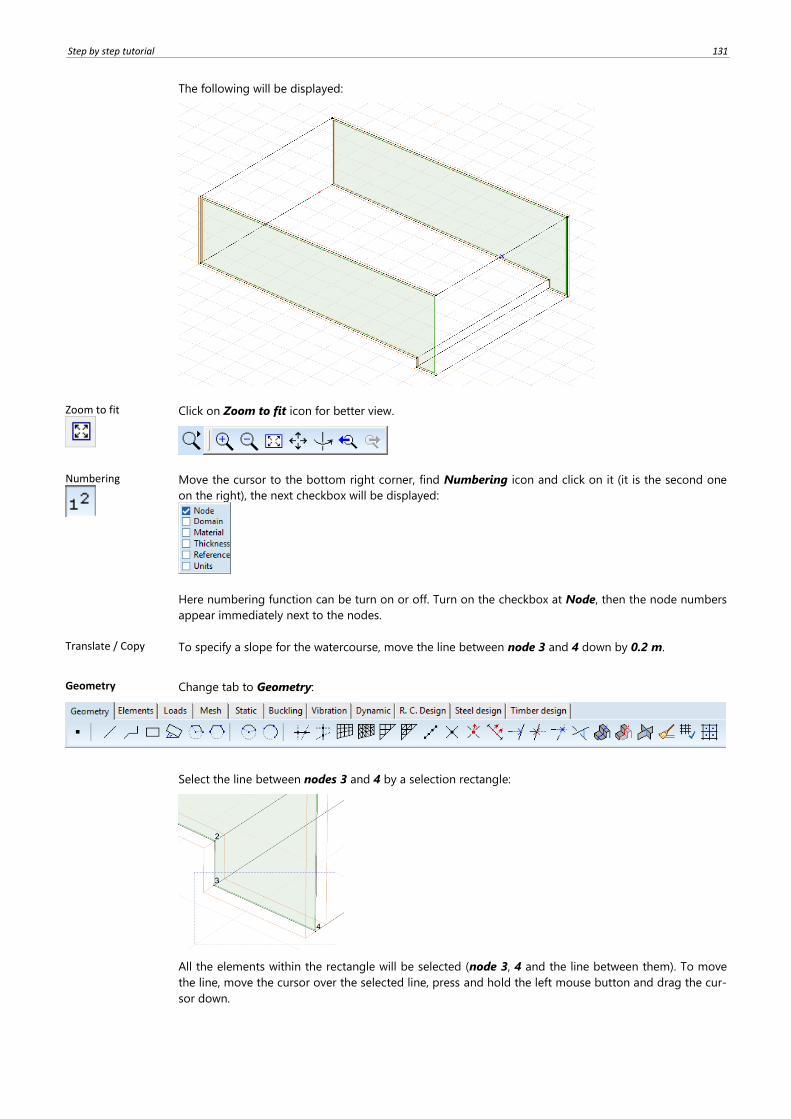
Step by step tutorial 131
The following will be displayed:
Zoom to fit
Click on Zoom to fit icon for better view.
Numbering
Move the cursor to the bottom right corner, find Numbering icon and click on it (it is the second one
on the right), the next checkbox will be displayed:
Here numbering function can be turn on or off. Turn on the checkbox at Node, then the node numbers
appear immediately next to the nodes.
Translate / Copy To specify a slope for the watercourse, move the line between node 3 and 4 down by 0.2 m.
Geometry Change tab to Geometry:
Select the line between nodes 3 and 4 by a selection rectangle:
All the elements within the rectangle will be selected (node 3, 4 and the line between them). To move
the line, move the cursor over the selected line, press and hold the left mouse button and drag the cur-
sor down.
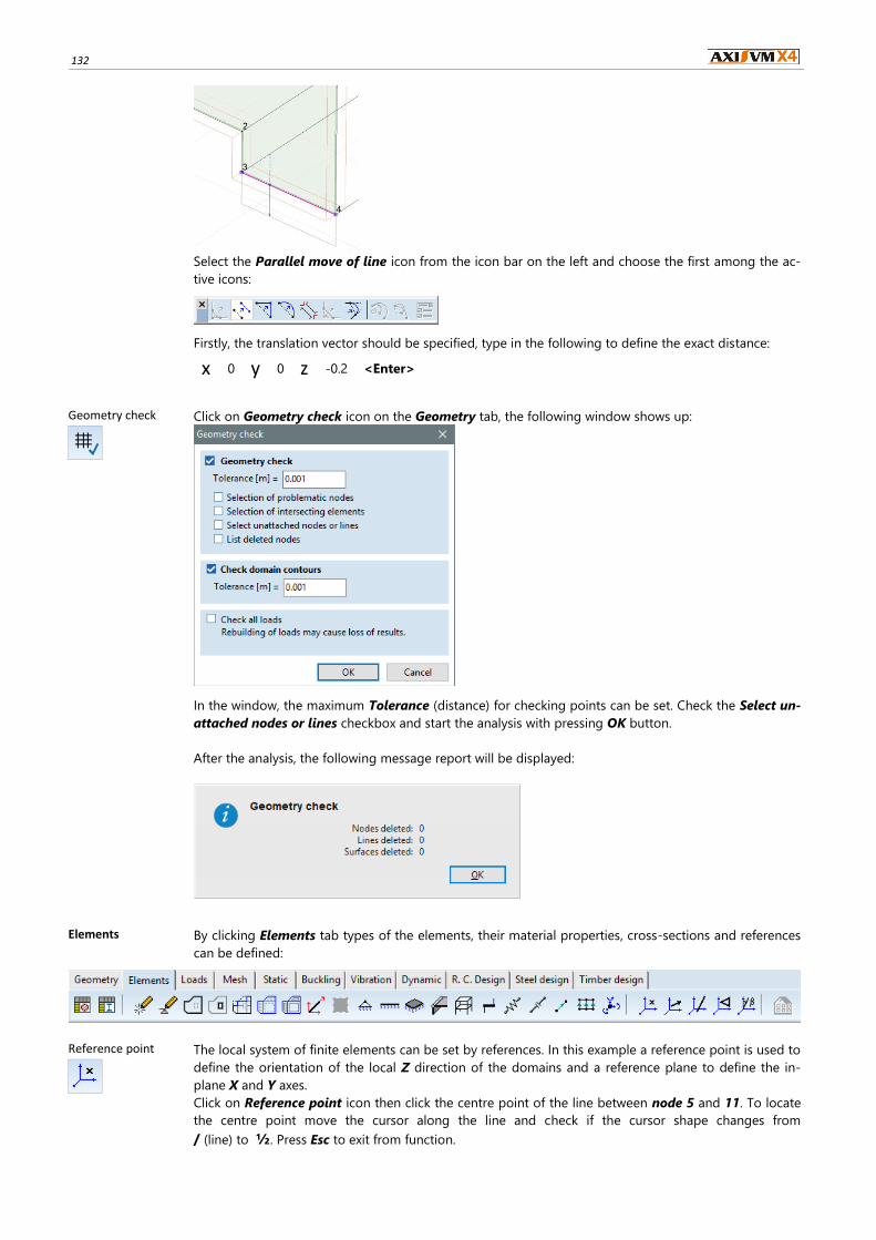
132
Select the Parallel move of line icon from the icon bar on the left and choose the first among the ac-
tive icons:
Firstly, the translation vector should be specified, type in the following to define the exact distance:
x 0 y 0 z -0.2 <Enter>
Geometry check
Click on Geometry check icon on the Geometry tab, the following window shows up:
In the window, the maximum Tolerance (distance) for checking points can be set. Check the Select un-
attached nodes or lines checkbox and start the analysis with pressing OK button.
After the analysis, the following message report will be displayed:
Elements By clicking Elements tab types of the elements, their material properties, cross-sections and references
can be defined:
Reference point
The local system of finite elements can be set by references. In this example a reference point is used to
define the orientation of the local Z direction of the domains and a reference plane to define the in-
plane X and Y axes.
Click on Reference point icon then click the centre point of the line between node 5 and 11. To locate
the centre point move the cursor along the line and check if the cursor shape changes from
/ (line) to ½. Press Esc to exit from function.
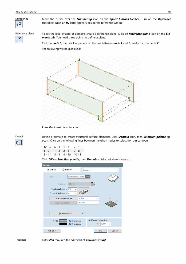
Step by step tutorial 133
Numbering
Move the cursor over the Numbering icon on the Speed buttons toolbar. Turn on the Reference
checkbox. Now, an R2 label appears beside the reference symbol.
Reference plane
To set the local system of domains create a reference plane. Click on Reference plane icon on the Ele-
ments tab. You need three points to define a plane.
Click on node 6, then click anywhere on the line between node 1 and 2, finally click on node 2.
The following will be displayed:
Press Esc to exit from function.
Domain
Define a domain to create structural surface elements. Click Domain icon, then Selection palette ap-
pears. Click on the following lines between the given nodes to select domain contours:
12 - 6 6 - 1 1 - 7 7 - 12
1 - 7 1 - 2 2 - 8 7 - 8
5 - 11 5 - 4 4 - 10 10 - 11
Click OK on Selection palette, then Domains dialog window shows up:
Thickness Enter 250 mm into the edit field of Thickness[mm].

134
Reference Set the Local x reference to R3:
then close window with OK.
A green contour can be seen along the domain boundary showing the shape of the domain. The colour
depends on the element type, shell domains always have a green contour.
Local systems Turn on the display of the local systems of Domains by clicking on the Local systems speed button in
the bottom right Speed buttons toolbar (fourth icon on the right).
Domain
Define the other wall elements. Click on Domain icon, then Selection palette appears and select lines
between the following nodes:
then finish selection with OK. Choose Shell element type and R3 for Local x reference and R2 for Lo-
cal z reference, finally press OK.
2 - 8 8 - 9 3 - 9 2 – 3,
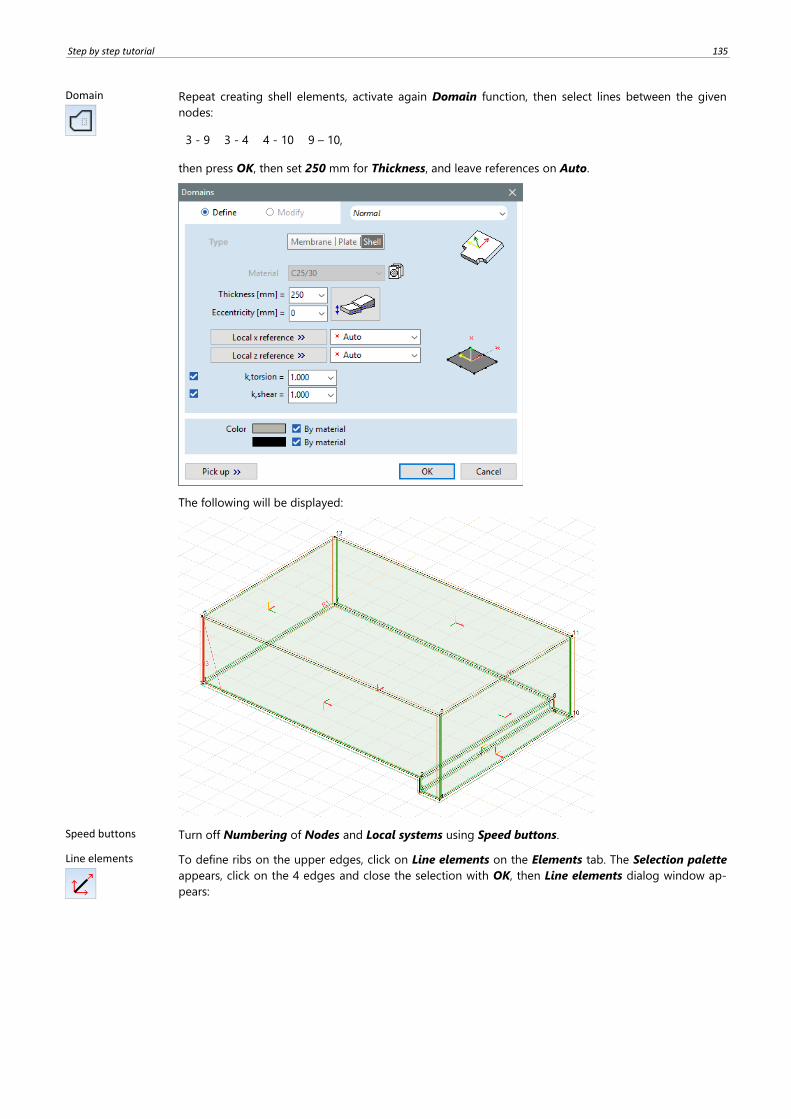
Step by step tutorial 135
Domain
Repeat creating shell elements, activate again Domain function, then select lines between the given
nodes:
then press OK, then set 250 mm for Thickness, and leave references on Auto.
3 - 9 3 - 4 4 - 10 9 – 10,
The following will be displayed:
Speed buttons Turn off Numbering of Nodes and Local systems using Speed buttons.
Line elements
To define ribs on the upper edges, click on Line elements on the Elements tab. The Selection palette
appears, click on the 4 edges and close the selection with OK, then Line elements dialog window ap-
pears:
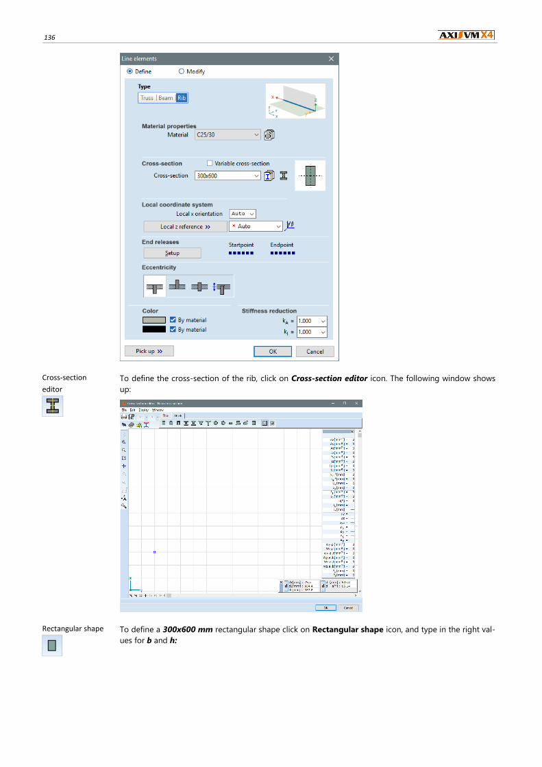
136
Cross-section
editor
To define the cross-section of the rib, click on Cross-section editor icon. The following window shows
up:
Rectangular shape
To define a 300x600 mm rectangular shape click on Rectangular shape icon, and type in the right val-
ues for b and h:

Step by step tutorial 137
Finishing the data input, press Place button to place the cross-section in the editor window. Click any-
where in the window. We get the next result:
The 1st and 2nd principal direction of the cross section indicated by the crossing dashed lines on the
cross-section, marked with numbers 1 and 2. The centre of gravity is marked with G. The other cross-
section parameters are displayed within the property window. Click More parameters if you want to see
all parameters calculated automatically by a finite element analysis of the shape.
Click OK to close Cross-section editor, in the dialog window change default name of cross-section if
required. Click on OK again to confirm.
Bottom rib
Set eccentricity to Bottom rib then finish settings with OK. Rib centre lines are displayed in blue and
the contour of the rib is shown in yellow.
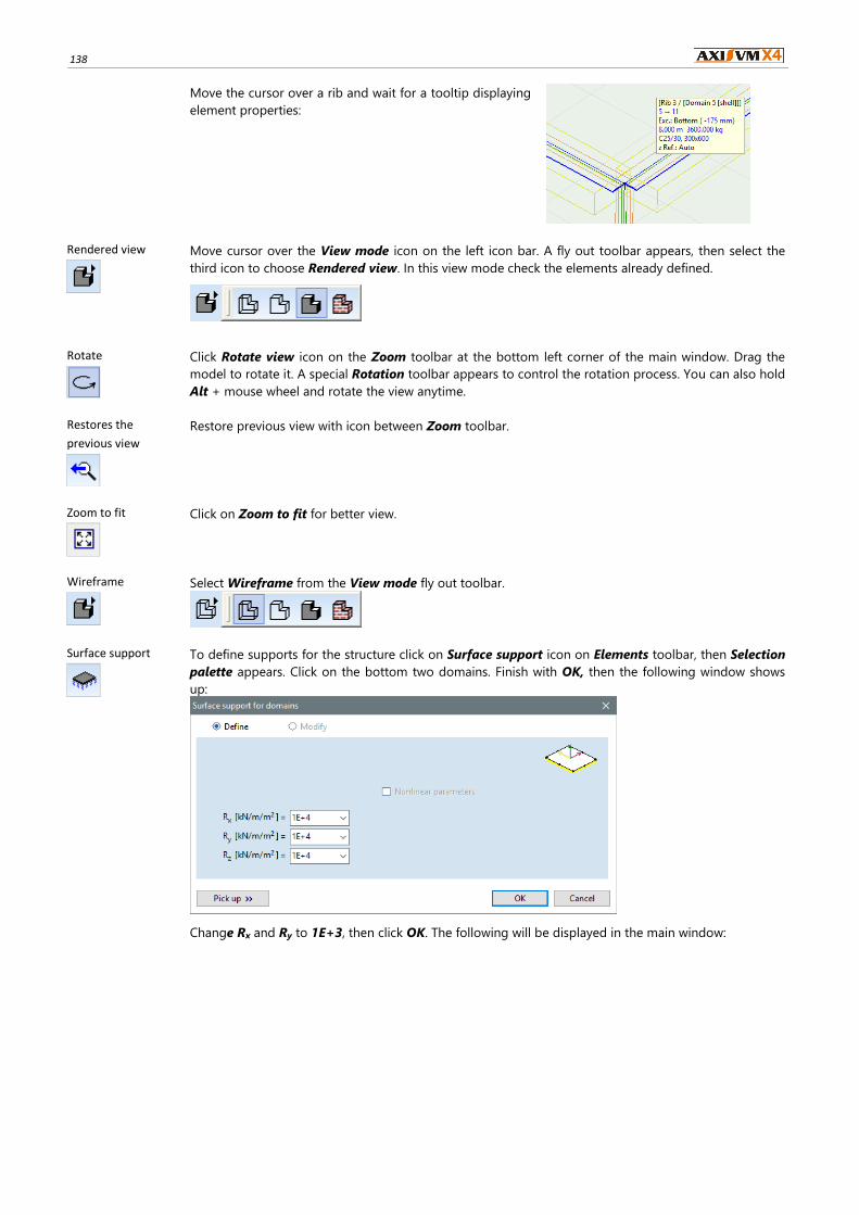
138
Move the cursor over a rib and wait for a tooltip displaying
element properties:
Rendered view
Move cursor over the View mode icon on the left icon bar. A fly out toolbar appears, then select the
third icon to choose Rendered view. In this view mode check the elements already defined.
Rotate
Click Rotate view icon on the Zoom toolbar at the bottom left corner of the main window. Drag the
model to rotate it. A special Rotation toolbar appears to control the rotation process. You can also hold
Alt + mouse wheel and rotate the view anytime.
Restores the
previous view
Restore previous view with icon between Zoom toolbar.
Zoom to fit
Click on Zoom to fit for better view.
Wireframe
Select Wireframe from the View mode fly out toolbar.
Surface support
To define supports for the structure click on Surface support icon on Elements toolbar, then Selection
palette appears. Click on the bottom two domains. Finish with OK, then the following window shows
up:
Change Rx and Ry to 1E+3, then click OK. The following will be displayed in the main window:
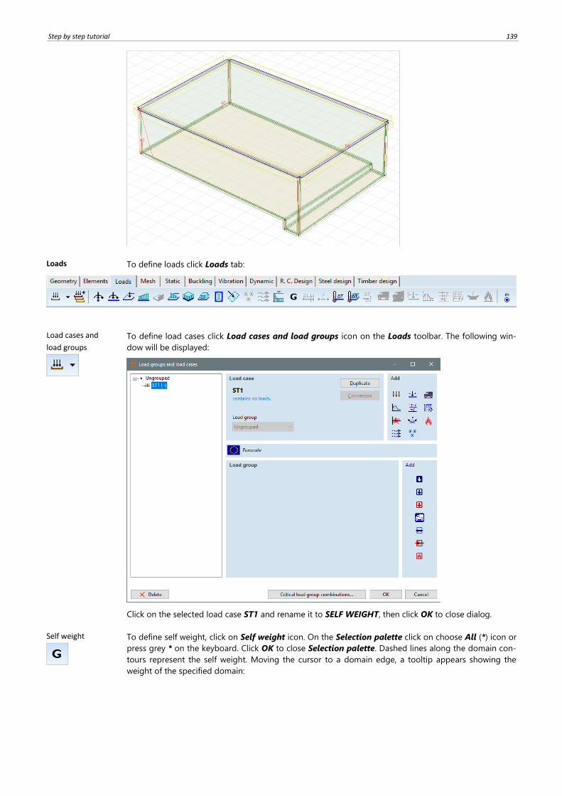
Step by step tutorial 139
Loads To define loads click Loads tab:
Load cases and
load groups
To define load cases click Load cases and load groups icon on the Loads toolbar. The following win-
dow will be displayed:
Click on the selected load case ST1 and rename it to SELF WEIGHT, then click OK to close dialog.
Self weight
To define self weight, click on Self weight icon. On the Selection palette click on choose All (*) icon or
press grey * on the keyboard. Click OK to close Selection palette. Dashed lines along the domain con-
tours represent the self weight. Moving the cursor to a domain edge, a tooltip appears showing the
weight of the specified domain:
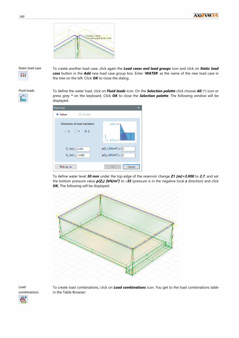
140
Static load case
To create another load case, click again the Load cases and load groups icon and click on Static load
case button in the Add new load case group box. Enter ’WATER’ as the name of the new load case in
the tree on the left. Click OK to close the dialog.
Fluid loads
To define the water load, click on Fluid loads icon. On the Selection palette click choose All (*) icon or
press grey * on the keyboard. Click OK to close the Selection palette. The following window will be
displayed:
To define water level 30 mm under the top edge of the reservoir change Z1 [m]=3.000 to 2.7, and set
the bottom pressure value p(Z2) [kN/m2] to –35 (pressure is in the negative local z direction) and click
OK. The following will be displayed:
Load
combinations
To create load combinations, click on Load combinations icon. You get to the load combinations table
in the Table Browser:

Step by step tutorial 141
New row
To create new load combinations, click on New row icon. Leave the name on default Co.#1 then select:
– (user defined combination). Then enter 1.35 into the column of case SELF WEIGHT and 1.00 into
the column of WATER load case. Use Tab or Enter to jump to the next cell. Click OK to close the dialog.
Speed buttons Use the speed buttons: turn off Supports, Reference and Object contours in 3D on Graphic symbols
tab.
Mesh To create finite element mesh change tab to Mesh.
Speed buttons Using speed button turn off Load display (the fifth icon on the right).
Domain meshing
Click on Domain meshing icon. On Selection palette click Select all (*) icon or press grey * on the
keyboard. Click on OK to close the Selection palette. Select rectangular mesh type (in centre) and set
Average Mesh Element Size to 0.60 m.
Click on OK to close dialog. Meshing process is can be followed on the status bar:
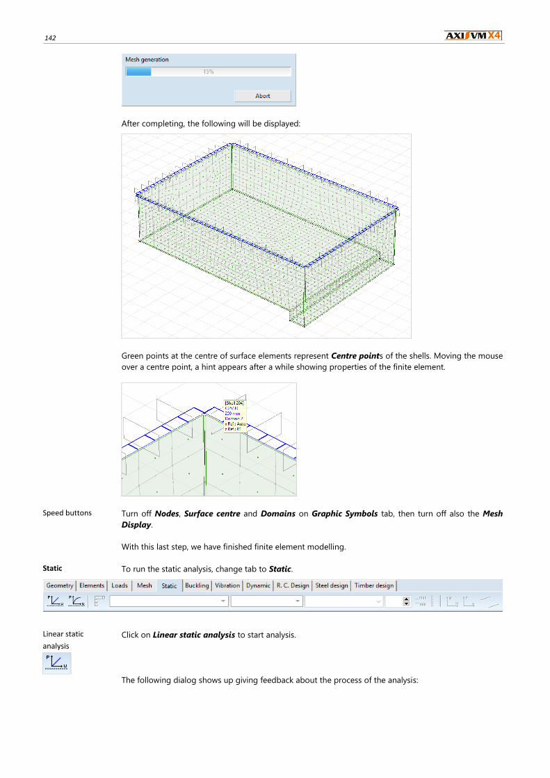
142
After completing, the following will be displayed:
Green points at the centre of surface elements represent Centre points of the shells. Moving the mouse
over a centre point, a hint appears after a while showing properties of the finite element.
Speed buttons Turn off Nodes, Surface centre and Domains on Graphic Symbols tab, then turn off also the Mesh
Display.
With this last step, we have finished finite element modelling.
Static To run the static analysis, change tab to Static.
Linear static
analysis
Click on Linear static analysis to start analysis.
The following dialog shows up giving feedback about the process of the analysis:
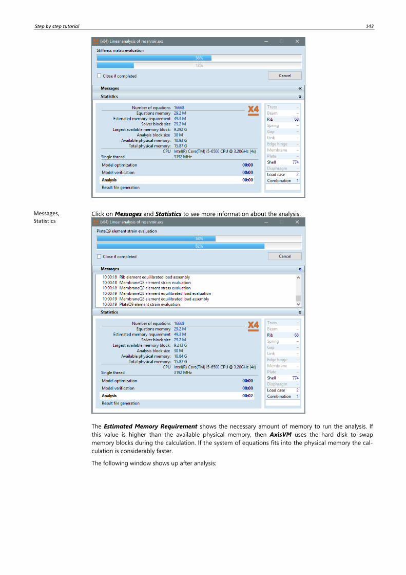
Step by step tutorial 143
Messages, Statistics
Click on Messages and Statistics to see more information about the analysis:
The Estimated Memory Requirement shows the necessary amount of memory to run the analysis. If
this value is higher than the available physical memory, then AxisVM uses the hard disk to swap
memory blocks during the calculation. If the system of equations fits into the physical memory the cal-
culation is considerably faster.
The following window shows up after analysis:
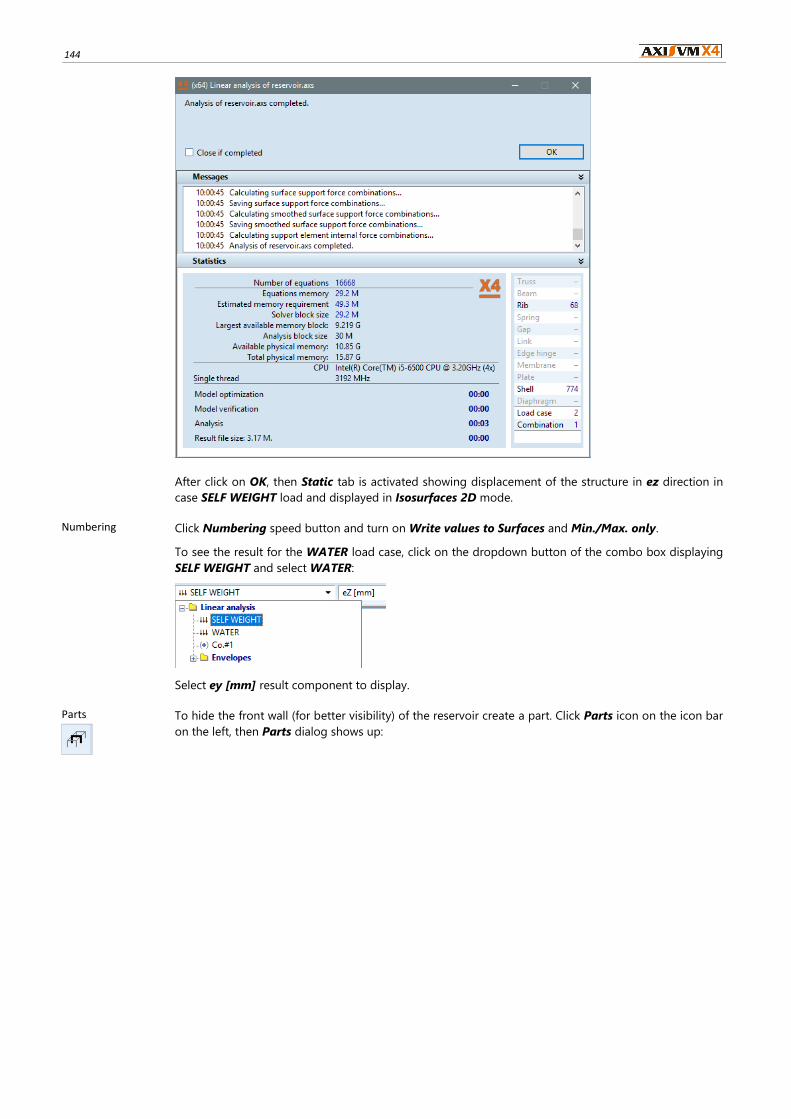
144
After click on OK, then Static tab is activated showing displacement of the structure in ez direction in
case SELF WEIGHT load and displayed in Isosurfaces 2D mode.
Numbering Click Numbering speed button and turn on Write values to Surfaces and Min./Max. only.
To see the result for the WATER load case, click on the dropdown button of the combo box displaying
SELF WEIGHT and select WATER:
Select ey [mm] result component to display.
Parts
To hide the front wall (for better visibility) of the reservoir create a part. Click Parts icon on the icon bar
on the left, then Parts dialog shows up:
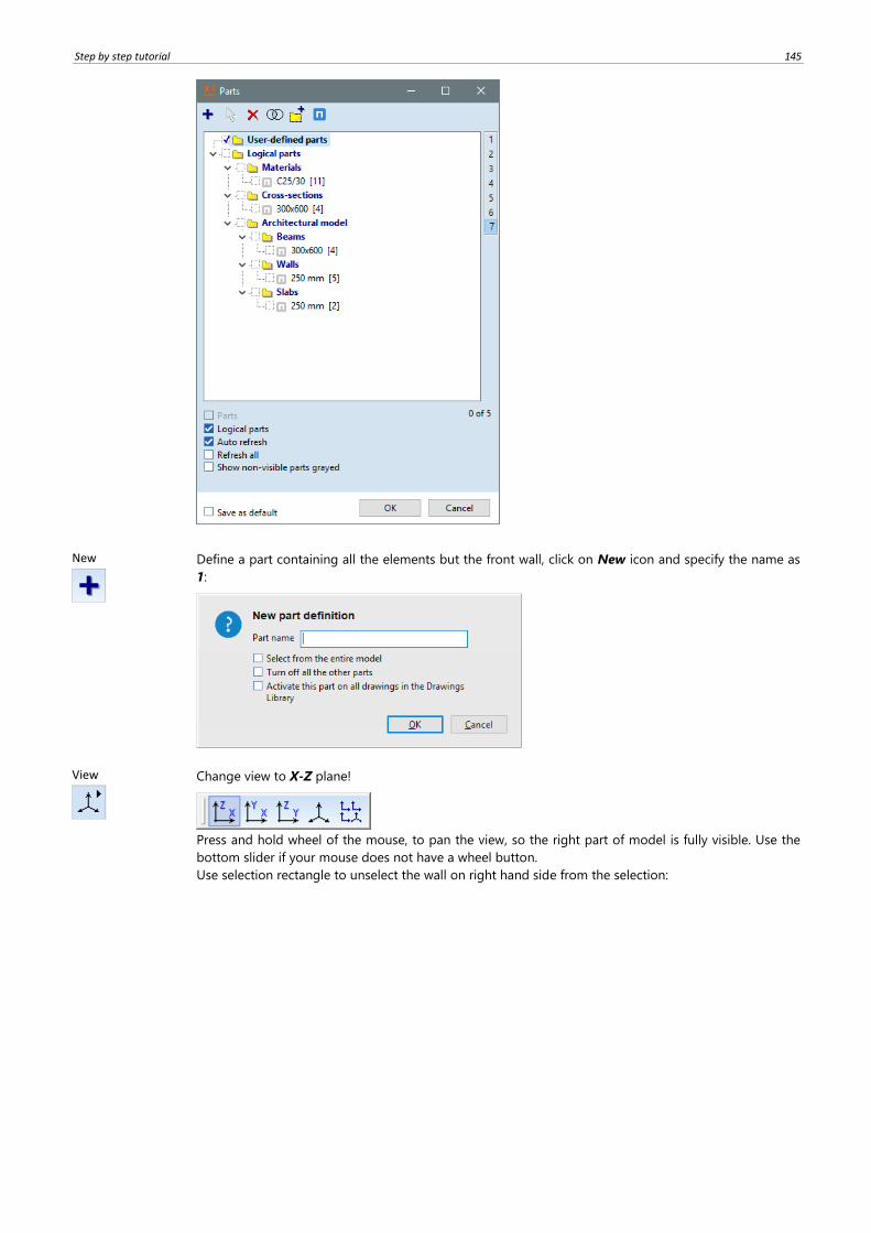
Step by step tutorial 145
New
Define a part containing all the elements but the front wall, click on New icon and specify the name as
1:
View
Change view to X-Z plane!
Press and hold wheel of the mouse, to pan the view, so the right part of model is fully visible. Use the
bottom slider if your mouse does not have a wheel button.
Use selection rectangle to unselect the wall on right hand side from the selection:

146
Click on OK on the Selection palette, then close Parts dialog window with OK.
Restore the
previous view
Restore the previous view with clicking the icon among Zoom toolbar – or activate Perspective view
with Ctrl+4 keys. Defining the part, the front wall is not visible in the next view:
Min, max values
To find extreme values of horizontal displacements, click Min, max values icon. The following window
shows up:
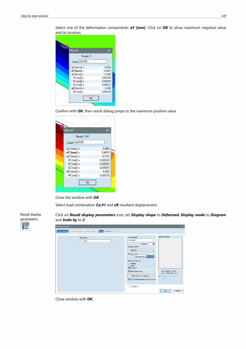
Step by step tutorial 147
Select one of the deformation components: eY [mm]. Click on OK to show maximum negative value
and its location.
Confirm with OK, then result dialog jumps to the maximum positive value.
Close the window with OK.
Select load combination Co.#1 and eR resultant displacement.
Result display parameters
Click on Result display parameters icon, set Display shape to Deformed, Display mode to Diagram
and Scale by to 2:
Close window with OK.
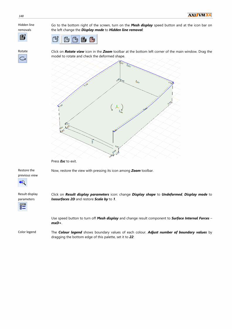
148
Hidden line
removals
Go to the bottom right of the screen, turn on the Mesh display speed button and at the icon bar on
the left change the Display mode to Hidden line removal:
Rotate
Click on Rotate view icon in the Zoom toolbar at the bottom left corner of the main window. Drag the
model to rotate and check the deformed shape.
Press Esc to exit.
Restore the
previous view
Now, restore the view with pressing its icon among Zoom toolbar.
Result display
parameters
Click on Result display parameters icon: change Display shape to Undeformed, Display mode to
Isosurfaces 2D and restore Scale by to 1.
Use speed button to turn off Mesh display and change result component to Surface Internal Forces –
mxD+.
Color legend The Colour legend shows boundary values of each colour. Adjust number of boundary values by
dragging the bottom edge of this palette, set it to 22:
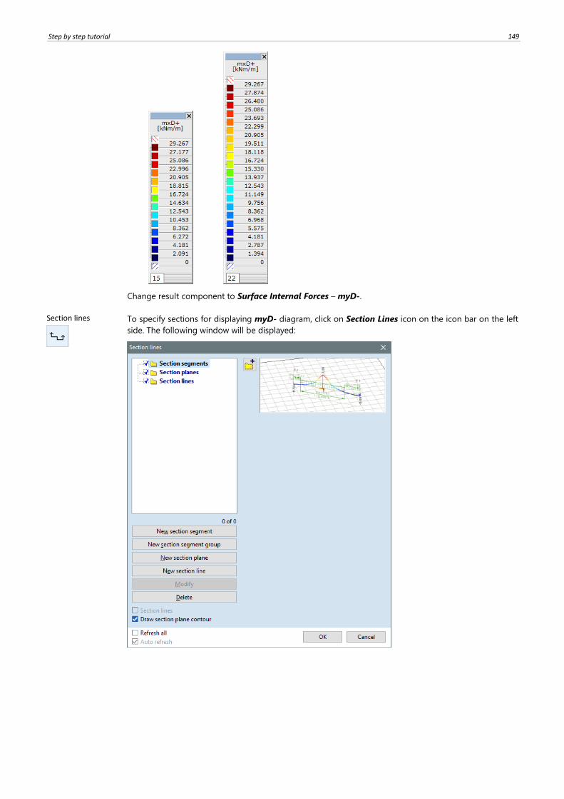
Step by step tutorial 149
Change result component to Surface Internal Forces – myD-.
Section lines
To specify sections for displaying myD- diagram, click on Section Lines icon on the icon bar on the left
side. The following window will be displayed:
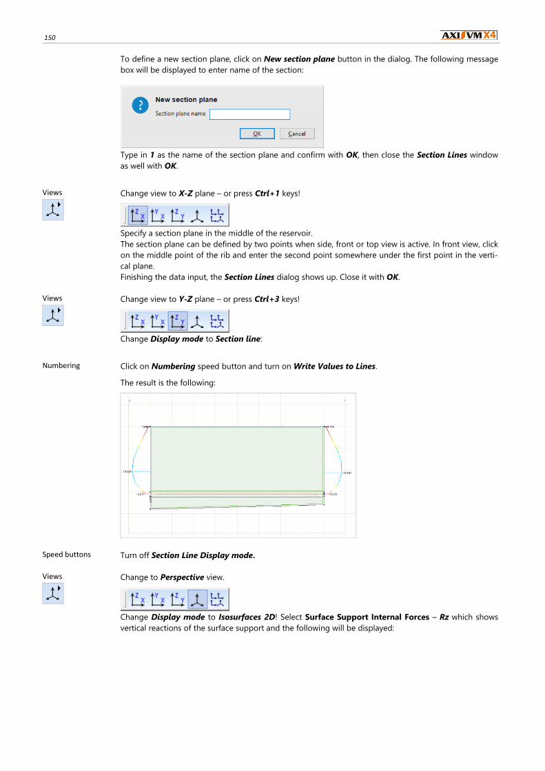
150
To define a new section plane, click on New section plane button in the dialog. The following message
box will be displayed to enter name of the section:
Type in 1 as the name of the section plane and confirm with OK, then close the Section Lines window
as well with OK.
Views
Change view to X-Z plane – or press Ctrl+1 keys!
Specify a section plane in the middle of the reservoir.
The section plane can be defined by two points when side, front or top view is active. In front view, click
on the middle point of the rib and enter the second point somewhere under the first point in the verti-
cal plane.
Finishing the data input, the Section Lines dialog shows up. Close it with OK.
Views
Change view to Y-Z plane – or press Ctrl+3 keys!
Change Display mode to Section line:
Numbering Click on Numbering speed button and turn on Write Values to Lines.
The result is the following:
Speed buttons Turn off Section Line Display mode.
Views
Change to Perspective view.
Change Display mode to Isosurfaces 2D! Select Surface Support Internal Forces – Rz which shows
vertical reactions of the surface support and the following will be displayed:
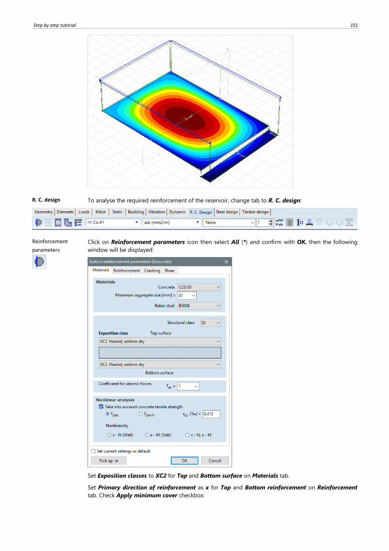
Step by step tutorial 151
R. C. design To analyse the required reinforcement of the reservoir, change tab to R. C. design:
Reinforcement
parameters
Click on Reinforcement parameters icon then select All (*) and confirm with OK, then the following
window will be displayed:
Set Exposition classes to XC2 for Top and Bottom surface on Materials tab.
Set Primary direction of reinforcement as x for Top and Bottom reinforcement on Reinforcement
tab. Check Apply minimum cover checkbox:
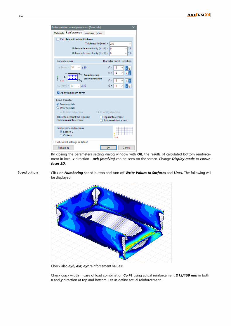
152
By closing the parameters setting dialog window with OK, the results of calculated bottom reinforce-
ment in local x direction - axb [mm2/m] can be seen on the screen. Change Display mode to Isosur-
faces 2D.
Speed buttons Click on Numbering speed button and turn off Write Values to Surfaces and Lines. The following will
be displayed:
Check also ayb, axt, ayt reinforcement values!
Check crack width in case of load combination Co.#1 using actual reinforcement Ø12/150 mm in both
x and y direction at top and bottom. Let us define actual reinforcement.
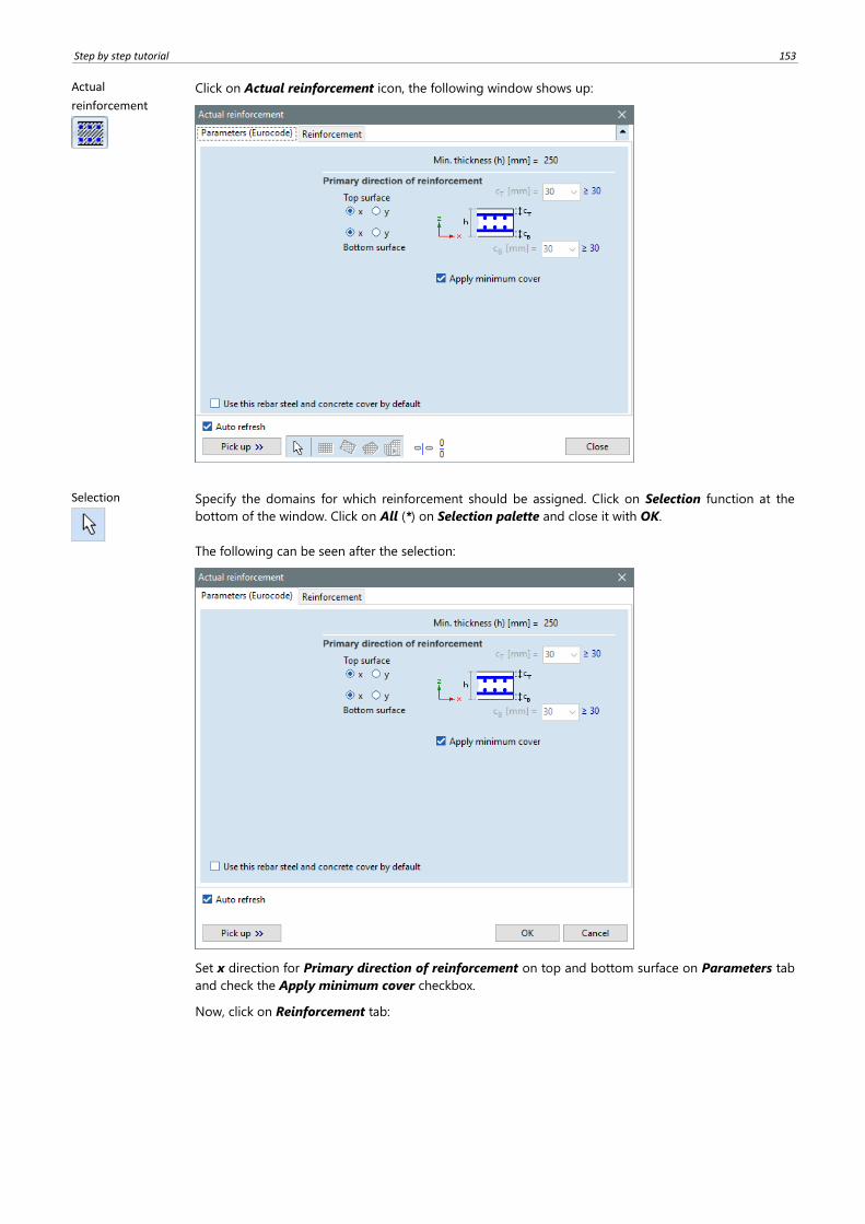
Step by step tutorial 153
Actual
reinforcement
Click on Actual reinforcement icon, the following window shows up:
Selection
Specify the domains for which reinforcement should be assigned. Click on Selection function at the
bottom of the window. Click on All (*) on Selection palette and close it with OK.
The following can be seen after the selection:
Set x direction for Primary direction of reinforcement on top and bottom surface on Parameters tab
and check the Apply minimum cover checkbox.
Now, click on Reinforcement tab:
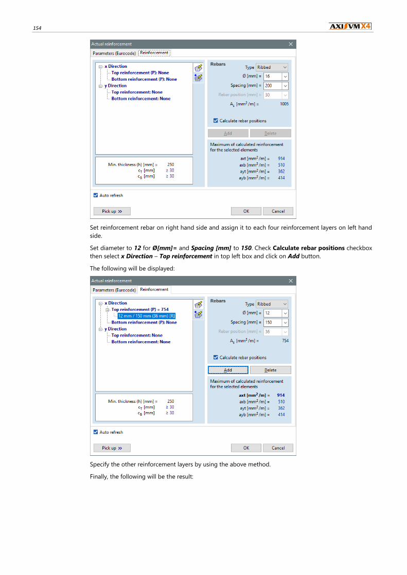
154
Set reinforcement rebar on right hand side and assign it to each four reinforcement layers on left hand
side.
Set diameter to 12 for Ø[mm]= and Spacing [mm] to 150. Check Calculate rebar positions checkbox
then select x Direction – Top reinforcement in top left box and click on Add button.
The following will be displayed:
Specify the other reinforcement layers by using the above method.
Finally, the following will be the result:
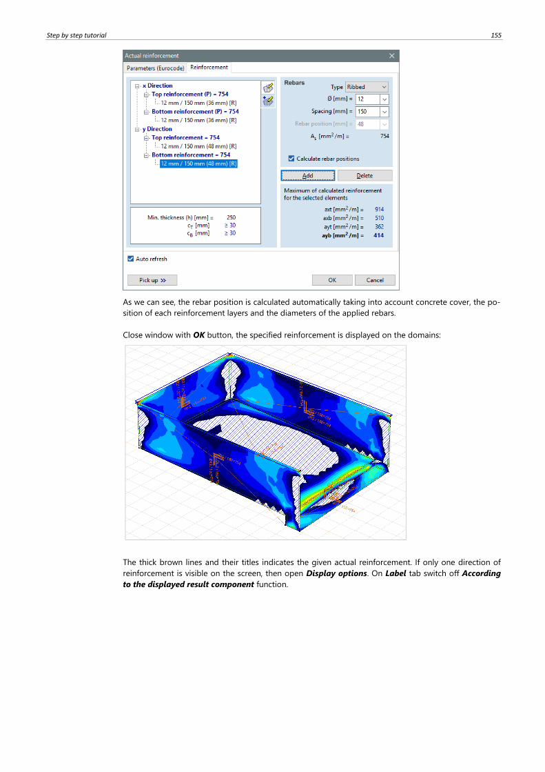
Step by step tutorial 155
As we can see, the rebar position is calculated automatically taking into account concrete cover, the po-
sition of each reinforcement layers and the diameters of the applied rebars.
Close window with OK button, the specified reinforcement is displayed on the domains:
The thick brown lines and their titles indicates the given actual reinforcement. If only one direction of
reinforcement is visible on the screen, then open Display options. On Label tab switch off According
to the displayed result component function.
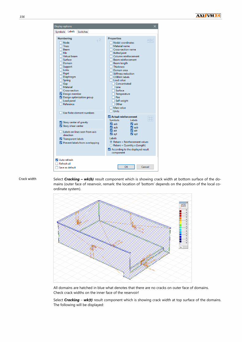
156
Crack width Select Cracking – wk(b) result component which is showing crack width at bottom surface of the do-
mains (outer face of reservoir, remark: the location of ’bottom’ depends on the position of the local co-
ordinate system).
All domains are hatched in blue what denotes that there are no cracks on outer face of domains.
Check crack widths on the inner face of the reservoir!
Select Cracking – wk(t) result component which is showing crack width at top surface of the domains.
The following will be displayed:
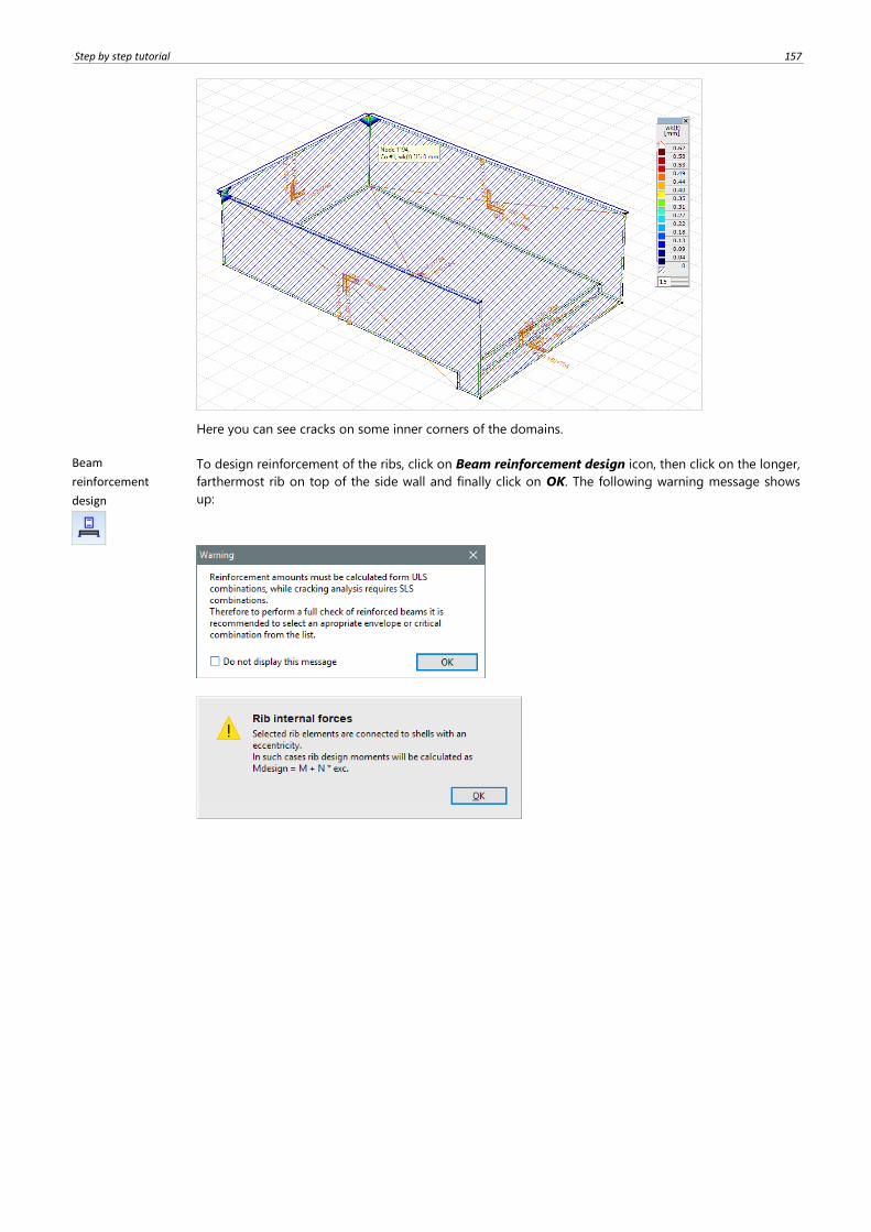
Step by step tutorial 157
Here you can see cracks on some inner corners of the domains.
Beam
reinforcement
design
To design reinforcement of the ribs, click on Beam reinforcement design icon, then click on the longer,
farthermost rib on top of the side wall and finally click on OK. The following warning message shows
up:
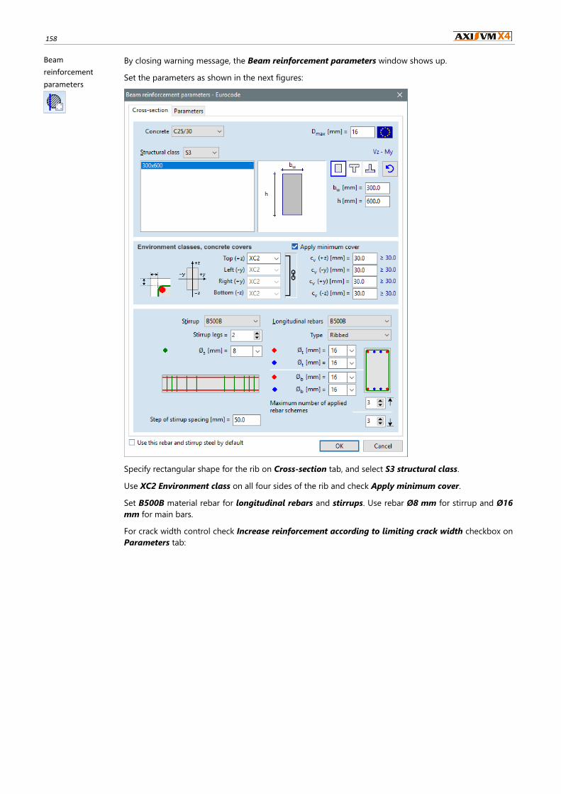
158
Beam
reinforcement
parameters
By closing warning message, the Beam reinforcement parameters window shows up.
Set the parameters as shown in the next figures:
Specify rectangular shape for the rib on Cross-section tab, and select S3 structural class.
Use XC2 Environment class on all four sides of the rib and check Apply minimum cover.
Set B500B material rebar for longitudinal rebars and stirrups. Use rebar Ø8 mm for stirrup and Ø16
mm for main bars.
For crack width control check Increase reinforcement according to limiting crack width checkbox on
Parameters tab:
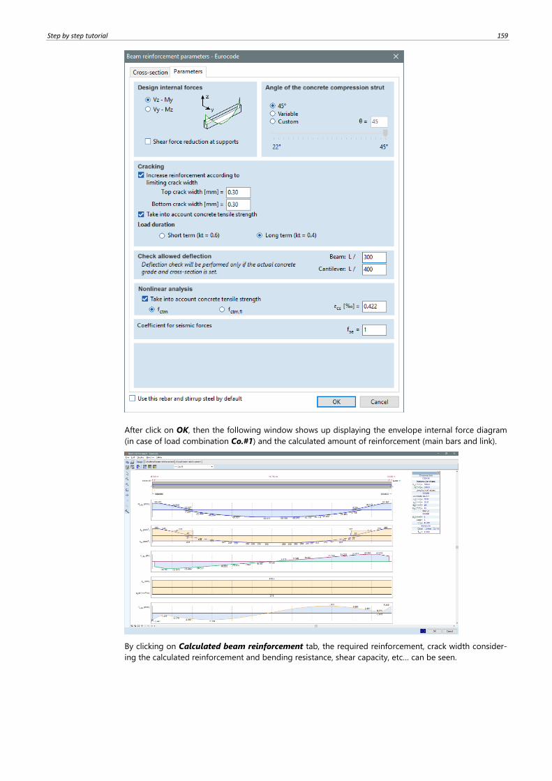
Step by step tutorial 159
After click on OK, then the following window shows up displaying the envelope internal force diagram
(in case of load combination Co.#1) and the calculated amount of reinforcement (main bars and link).
By clicking on Calculated beam reinforcement tab, the required reinforcement, crack width consider-
ing the calculated reinforcement and bending resistance, shear capacity, etc… can be seen.
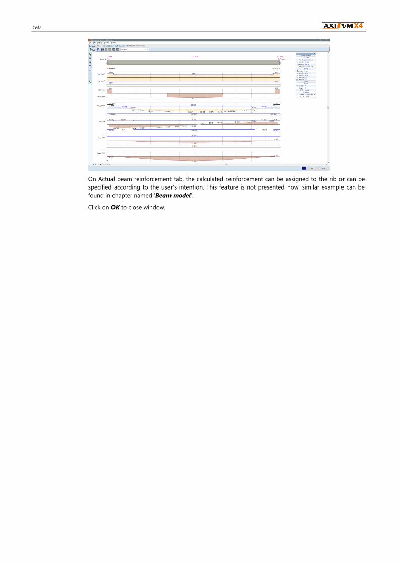
160
On Actual beam reinforcement tab, the calculated reinforcement can be assigned to the rib or can be
specified according to the user’s intention. This feature is not presented now, similar example can be
found in chapter named ‘Beam model’.
Click on OK to close window.

Step by step tutorial 161
Notes

162
Notes