Embed Size (px)
Citation preview


S T E P - B Y - S T E P U S E R G U I D E
Mastering the SIGÉOM Data
http://sigeom.mines.gouv.qc.ca
Gouvernment of Québec Ministère de l’Énergie et des Ressources naturelles
General Direction of Géologie Québec
Version : February 2019
This document describes three ways to access the data in SIGÉOM using the same functions in three different work environments. Reading this document is like reading a cookbook: step by step. At the end of this exercise, you will be able to master the SIGÉOM data.

Table of contents
1. INTRODUCTION 3
2. THE INTERACTIVE MAP 4
2.1 Access to Data 4
2.2 Layer Display 6
2.3 Displaying Geophysical Data 9
2.4 Adding Data from External Sources 10
2.5 Relational Data Model 10
2.6 Querying the Data 11
2.7 Data Editing 13
2.8 Dynamic Location 14
2.9 Location with a Coordinate 15
2.10 Placing a Freehand Marker 17
2.11 Sharing the Map 18
2.12 Searching for Gold Anomalies in
Drilling 20
2.13 Printing 22
3. DATA LAYER 23
3.1 Types of Geometric Layouts of
Layers 23
3.2 Extracting Data Layers from SIGÉOM 24
3.3 Symbology of Layers 25
3.4 Coordinate System 26
4. QGIS – FREE GIS SOFTWARE
(GEOGRAPHICAL INFORMATION SYSTEM) 27
4.1 Cost 27
4.2 Installation 27
4.3 Access to Data 29
4.4 Layer Display in QGIS 31
4.4.1 Project Preparation 31
4.4.2 Import Shapefiles (Form Files) and an
Entity Class from a FGDB 32
4.4.3 Changing the Colours of Geological
Zones 35
4.5 Display of Geophysics 42
4.6 Adding Data from External Sources 45
4.6.1 Import a Map Background to the Project 45
4.6.2 Import Data from a Microsoft Excel
Spreadsheet 47
4.7 Relational Data Model 49
4.8 Querying Data 49
4.9 Editing Data 52
4.10 Dynamic Location 52
4.11 Location with Coordinates 53
4.12 Place a Freehand Marker 53
4.13 Sharing a Map 54
4.14 Looking for Gold Anomalies in
Drillings 54
4.14.1 With QGIS 54
4.14.2 With SIGÉOM à la carte 59
4.15 Printing 61
5. ESRI FGDB FORMAT 62
5.1 Cost 62
5.2 Access to Data 62
5.3 Layer Display 62
5.4 Display of Geophysics 63
5.5 Adding Data from External Sources 65
5.6 Import Data from a Microsoft Excel
Spreadsheet 66
5.7 Relational Data Model 69
5.8 Querying Data 71
5.9 Data Editing 77
5.10 Dynamic Location 78
5.11 Location with Coordinates 80
5.12 Sharing a Map 81
5.13 Looking for Gold Anomalies in
Drillings 84
5.14 Printing 88
5.15 Difference Between Shapefile and
FGDB 89
CONCLUSION 91
Comparison Table 92
CONTACT US 93
APPENDIX 1 – SITE SELECTION METHODS
(SPATIAL QUERIES) 94
APPENDIX 2 – DATA AND COORDINATE
SYSTEM 103
ArcGIS Software 103
Change the coordinate system at the source 103
Change the coordinate system for viewing 104
QGIS Software 104
Change the coordinate system for viewing 104
APPENDIX 3 – LIST OF LINKS 105
WMS Mapping Services 105
Others 105

3
1. Introduction
SIGÉOM data is a rich Quebec heritage. They cover more than 150 years of geoscience surveys and combine information and surveys from government, mining exploration companies, academic researchers and other sources. We estimate that this collective wealth represents an undiscounted value of $4.4 billion.
SIGÉOM, whose first map was produced in 1993, has changed over the years, as have the formats for accessing and processing data provided. The 1993 customer offer, although not exhaustive, was published in Bentley’s digital DGN format. Today, this offer has evolved into formats and modes of consultation that enable the acquisition and visualization of all the information available in SIGÉOM in terms of descriptive and geometric data. Information can also be accessed using the latest Internet technologies such as the Web Map Service (WMS) or the Interactive Map.
The purpose of this document is to guide the user in the choice of different access modes to the data so that they can compare them, understand the advantages and limitations of each technology (format) available. This guide is intended for all users of SIGÉOM, from the occasional user looking for general information on the geology of Quebec, through the geomatics professional who wants to compare data access technologies.
A summary table at the end of this guide compares the results obtained for the various functions presented. We designed this guide as a recipe book so that the reader could follow the steps and repeat them. We also recognize that we do not address all aspects of each technology and hope to improve this guide based on user feedback and enrich it over time.
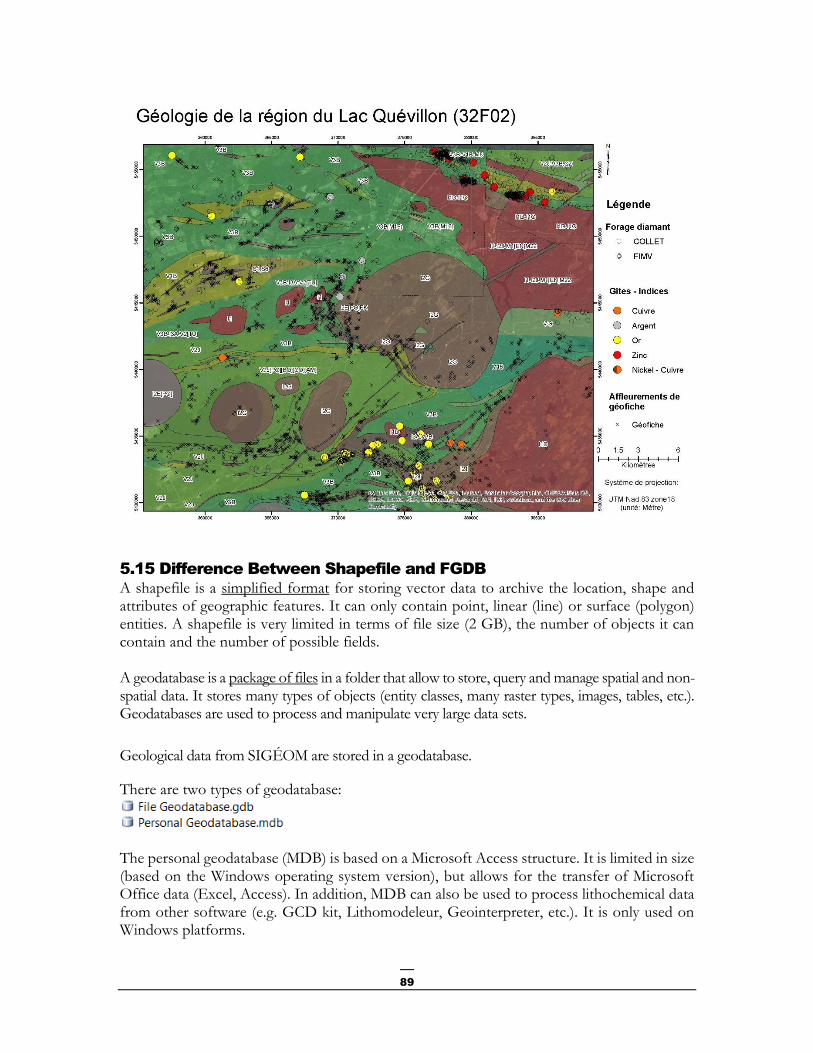
The territory chosen for this guide covers NTS sheet 32F02, an area northeast of Val-d'Or near the town of Lebel-sur-Quévillon. This territory contains enough data to provide good examples, particularly for mineralization research. We have included some data that are available on the Ministère de l’Énergie et des Ressources naturelles FTP site, with the exception of sheet 32F02 geology data that can be obtained from the SIGÉOM website.
It is our hope that this guide will allow you to discover the richness of SIGÉOM geoscientific data and make it your own by choosing the format and/or technology that works for you.

4
2. The Interactive Map
The interactive map is Géologie Québec’s web mapping application. This interactive map, available free of charge, allows you to locate and visualize a multitude of geological and mining data on the Quebec territory (geological units, mineral deposits, diamond drillings, mines and projects, etc.) and to link it to mining information (mining activities, mining titles) and geographic information (satellite images, hydrography, topography, etc.). The use of the interactive map does not require any installation.
This map is compatible with Microsoft Internet 8+, Google Chrome 20+, Firefox 14+ Windows and Mac OS browsers.
During this demonstration, the Google Chrome 34 browser in Windows XP is used.
2.1 Access to Data
Consultation of the interactive map is free and does not require any authentication.
Direct URL: http://carte-geomine.mrn.gouv.qc.ca
OR
From the Ministère page: http://www.mern.gouv.qc.ca/
in the horizontal menu bar, click the mines tab:
in the right section, under Quick links, click SIGÉOM

5
on the SIGÉOM home page, click on Access to open the interactive map.
The page is divided into three sections:
The menu
The map section
The location section
3
2
1

6
2.2 Layer Display
1. From the References menu, check the NTS mapsheet layer.
2. Click the Zoom in tool for a larger view of the selected area.
3. Expand the area of sheet 32F. To do this, hold the left mouse button to delimit the contour of the area of interest.
4. Click the Zoom in tool again and frame sheet 32F02 to outline the enlargement contour.

7
5. In the Data layers menu
Check off the following layers:
Use the slide bar to adjust
the transparency of the
layer.
The icon opens the
legend at the top of the
map on the right. To close
the legend, click on the
in the window.
The interactive map offers
simplified symbolization
compared to that used in
SIGÉOM à la carte.
The download
icon creates a
png image of the
legend.

8

9
2.3 Displaying Geophysical Data
Static layers are matrix images that are usually the result of data synthesis. They are updated once a year.
In the Static layers menu, check the Vertical gradient of high resolution residual total magnetic
field layer.
In the Data layers menu, uncheck the Regional geology layer for a better view of the vertical gradient map.

10
2.4 Adding Data from External Sources
It is not possible to add external data layers of your choice.
However, a choice of basic maps is available for the topographic background. This data comes from Google and OpenStreetmap.
1. In the Static layers menu, uncheck the Vertical gradient of high resolution residual total
magnetic field layer.
2. Click the button
3. Click on the image to activate the Google
satellite layer.
4. Check the option to display the names of cities, roads, etc.
To return to the initial baseline map, click on the image
to activate the layer Google plan.
2.5 Relational Data Model
Not represented. Data is simplified.

11
2.6 Querying the Data
To query an item, simply click on an item on the screen using the left mouse button and view the information in the dialogue box.
The information displayed is a simplified version of the data found in SIGÉOM à la carte. For more detailed information, links are available for several types of items.
1. In the Data layers menu, uncheck the Geofiche outcrops (GO) and Regional faults layers to lighten the map.
2. Click on the Zoom in tool to get a larger view.
3. Enlarge the map of the area identified in the image below, on the top right. To do this, hold the left mouse button to delimit the area of interest.

12
4. Click on the Diamond drillings item , identified by orange arrows on the image below.
Note that the system displays information for all active layers and overlaid data.
5. In the information box, click on the 01-MFS-04EXT link of the second diamond drilling.
At this stage of the guide, we want to demonstrate the links that exist with SIGÉOM à la carte. A drilling other than 01-MFS-04EXT could be selected.

13
A new window opens and directs you to the corresponding item in SIGÉOM à la carte.
This page displays all the information available in SIGÉOM. It provides, among other things, access to Examine documents related to this drilling. A hyperlink is available pointing to GM59766 and allows access to the original document.
6. Close the page Géologie Québec – Results of the query.
When you return to the interactive map page, you can close the information box by clicking .
2.7 Data Editing
Data editing is not possible.

14
2.8 Dynamic Location
Text can be freely entered in the search field to look for a place, city, address or postal code.
1. In the Address, place, postal code field located in the Location section, type: bachelor and
click on .
The system zooms in on Lac Bachelor, Baie-James and creates a marker. Push the “Markers” button to access the markers' information box. Note that a List of markers is available.
A marker is a point created on the map with wording (name). Markers are retained as long as the internet browser is open.
It is possible to change the name, delete a marker or zoom in on a marker from the List of
markers information box.

15
2.9 Location with a Coordinate
It is possible to locate a point on the map from its coordinates. The system will zoom in on this location and place a marker.
1. Click on the button
2. Type the following values in the UTM section and click the Ok button (example of coordinates from document GM 59766):
X: 293460 Y: 5454639 Zone: 18
A new marker is added to the List of markers.

16
3. Select the default text from the last marker and delete it.
4. Replace the default name with GM 56766, drilling x by typing in the text box of the marker.
The wording (name) is automatically changed on the map.
17
2.10 Placing a Freehand Marker
1. Click the button if the markers' information box is not visible.
2. In the Freehand on the map section, click the button . The information box
closes and the cursor is replaced by .
If you do not see the Freehand on the map section, click on the button to expand the window.
3. Place a marker somewhere by clicking on the map. This new marker is added to the List of
markers.

18
2.11 Sharing the Map
It is possible to share your map as it appears on the screen with other users.
1. If necessary, close information boxes on the map by clicking on .
2. Zoom out to get an overview of the data and markers. To do this, use the slide bar of navigation tools or simply the mouse wheel.
In this example, the Regional geology, Regional faults, Metallic deposits and Diamond drillings layers were activated.
3. Click the button and select the first link.
4. Copy the selected link to a new web window to see the result. The map opens as it appears in the source window.
19
This example shows that the result is similar in both windows. These sharing links can be used to share information among collaborators, add a map to a blog, wiki or web page, etc.
Several ways to share the map
- sharing links via Facebook, Twitter and Google+
- Copy and paste a link: this field contains an URL that you can copy and paste into an email, an instant message (Facebook, Twitter, LinkIn, etc.) or add to a collaborative tool (blog, wiki).
- *Paste the HTML code to a website: you can copy and paste this HTML code to add the map to your website.

20
2.12 Searching for Gold Anomalies in Drilling
Using the search functions of SIGÉOM à la carte, gold anomalies in drilling can be identified. In this example, we will select drillings that contain an intermediate volcanics (V2) description with geochemical analysis exceeding a threshold of 1000 ppb (1 g/t) gold.
1. From the SIGÉOM à la carte homepage [http://sigeom.mines.gouv.qc.ca], click on the highlighted title in the Drilling/Diamond drilling section. You will be directed to the right place in the list of themes belonging to SIGÉOM.
Click on the desired topic of the theme (Diamond drilling) to submit the subject’s query form.
2. Enter the following values in the appropriate fields.

21
3. Click the Search button on the left hand menu to run the query.
4. Click the button on the left menu.
A new tab opens and the query generation is initiated. When completed, a zoom is applied to the elements of the Diamond drilling query.
By default, the symbol used to identify drillings that meet the criteria is an orange circle. You can change the colour of the queries by clicking on the button .
For the Diamond drilling query, click on the orange square and select a new colour.
A KML file (Keyhole Markup
Language) is generated for each
query made in SIGÉOM à la
carte. However, results of the
query must not exceed a limit.

22
2.13 Printing
To print the interactive map, use the Printscreen function on your keyboard.
There are several freewares available to save screenshots in different formats (PDF, jpeg, gif, png, etc.). Here are some links:
Picpick: http://www.picpick.org/en/
FastStone capture: http://www.faststone.org/FSCaptureDetail.htm
However, the Ministère de l’Énergie et des Ressources naturelles and Géologie Québec does not endorse or support these freeware programs in any way.

23
3. Data Layer
3.1 Types of Geometric Layouts of Layers
Entity classes represent homogeneous sets of common entities, all with the same spatial representation (such as points, lines or polygons) and a common set of attribute columns (descriptive). The four most commonly used types of layouts are points, lines, polygons and annotations (name of map text in geodatabases).
Entity Class Type
Points Entities too small to be represented as lines or polygons, and point locations (e.g. GPS observations).
Lines (polylines) Represent the shape and location of geographic objects too narrow to be displayed as surfaces. Lines can also represent entities that have a length but no surface, such as isolines and boundaries.
Polygons A set of surface features with many sides representing the shape and location of homogeneous entity types such as states, departments, parcels, soil types and land use zones.
Annotations Map text including text rendering properties. Annotations can also be linked to entities and contain subclasses.

24
3.2 Extracting Data Layers from SIGÉOM
Extracting SIGÉOM data is free and requires no authentication. For a layer order, please refer to the “Vector data and web Service” stream by clicking “SIGÉOM à la carte” on the home page.
Products offered via SIGÉOM:
Quebec-wide SIGÉOM database in FGDB format;
Quebec-wide SIGÉOM database in Shapefile (shp) format;
database by entity (à la carte data) with the ability to filter results using a query.
Products available through the Government of Quebec’s open data site (https://www.donneesquebec.ca):
Quebec-wide SIGÉOM database by entity group in FGDB format;
Quebec-wide SIGÉOM database by entity group in Shapefile (shp) format;
Note that within each entity group, a layer exists for each of the SIGÉOM entities.

25
3.3 Symbology of Layers
Symbols are graphic elements used in map views. There are four basic types of symbols:
Point symbols are used to display the position of points or embellish other types of
symbols.
Linear symbols are used to display linear boundaries and features.
Fill symbols are used to fill polygons or other surfaces such as map backgrounds.
Text symbols are intended for the font, size, colour and other properties of label and
annotation text.
The value of specifying the symbology of a layer in the project (not in the database) is to be able to modify it based on representation needs. ArcMap offers you the opportunity to use the information contained in the layer database to define how entities will be represented. A layer used in two different projects may have a different representation in each. A layer used several times in the same project may also have several different representations for each of its occurrences. The aspect you give your data will be very important in how the user may understand and use it. Symbols can be used to meet two needs:
The first, the most obvious, is the need for representation to produce a printed
document (a map). The choice of symbolization should allow the user to understand
the message the map is intended to convey.
The second need would be to facilitate various data work. For example, symbolization
may be modified to facilitate editing (adding or deleting entities), validations or data
inspections.
When retrieving data from SIGÉOM, symbology is unique to each of the layers of the .mxd project extraction. The information in this symbology is stored in the SIGEOM.style file in the extraction Symbolization folder. In the same folder, refer to the Installation.txt files for the use of this style file.

26
3.4 Coordinate System
SIGÉOM spatial data is designed in a system of specific coordinates, whether points, lines or polygons. It is therefore possible to consult the geometric information precisely using the coordinate system on Quebec territory.
Data extracted from SIGÉOM in SHAPEFILE and FGDB format are recorded in geographic coordinates in the geodetic reference system NAD83 based on the ellipsoid GRS80. It is possible to change the coordinate system at the data source or only when viewing the data in a GIS.
Refer to Annex 2 for different ways of doing this using ArcGIS and QGIS GIS softwares.

27
4. QGIS – Free GIS Software (Geographical Information
System)
QGIS provides the ability to visualize, create, edit, generate, explore and analyze data, and integrates many vector, matrix, database and other formats. It manages matrix image formats (GRASS GIS, GeoTIFF, TIFF, JPG, etc.) and vector data (Shapefile, ArcInfo, FGDB, Mapinfo, GRASS GIS, etc.) as well as databases.
4.1 Cost
GGIS is free and distributed under the GNU General Public Licence [http://fr.wikipedia.org/wiki/Licence_publique_generale_GNU].
4.2 Installation
QGIS is software designed to operate on multiple platforms. It is compatible with Windows, Linux, Unix, Mac OS X and Android.
For this demonstration, version 2.18 (Las Palmas) is used on Windows 7 Professional.
1. To download the software, go to:
https://www.qgis.org/fr/site/forusers/download.html
2. Select the download for your operating system, make sure you have the correct version.
Wait until the installation run file is uploaded to your station.
3. Select Run and follow the installation steps.

28
4. Start QGIS Desktop
5. You need to install the following extensions for the next demonstration:
GeoCoding (to find an address, a place)
Pin Point (to manually place a point)
ZoomToCoordinates (to zoom in on a coordinate area)
6. From the top menu of the window, click Plugins and Manage and Install Plugins…
7. For each extension, you must select it from the list and click Install plugin at the bottom right of the window.
8. When all three extensions are installed, close the window.

29
4.3 Access to Data
Access to SIGÉOM geomatics data (FGDB and Shapefile) is available at the following address: http://sigeom.mines.gouv.qc.ca/signet/classes/I1102_aLaCarte?l=A
Vector data are available individually via Data retrieval with SIGÉOM à la carte, or by NTS-sheet
number.
1. Click the button on the SIGÉOM à la carte page. In the search environment, enter the 32F02 NTS sheet number. Then, click Search from the menu on the left.
2. Click on Download (FGDB/SHP) from the left menu.
30
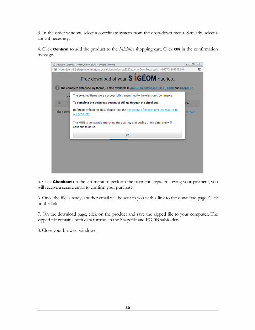
3. In the order window, select a coordinate system from the drop-down menu. Similarly, select a zone if necessary.
4. Click Confirm to add the product to the Ministère shopping cart. Click OK in the confirmation message.
5. Click Checkout on the left menu to perform the payment steps. Following your payment, you will receive a secure email to confirm your purchase.
6. Once the file is ready, another email will be sent to you with a link to the download page. Click on the link.
7. On the download page, click on the product and save the zipped file to your computer. The zipped file contains both data formats in the Shapefile and FGDB subfolders.
8. Close your browser windows.
31
4.4 Layer Display in QGIS
4.4.1 Project Preparation
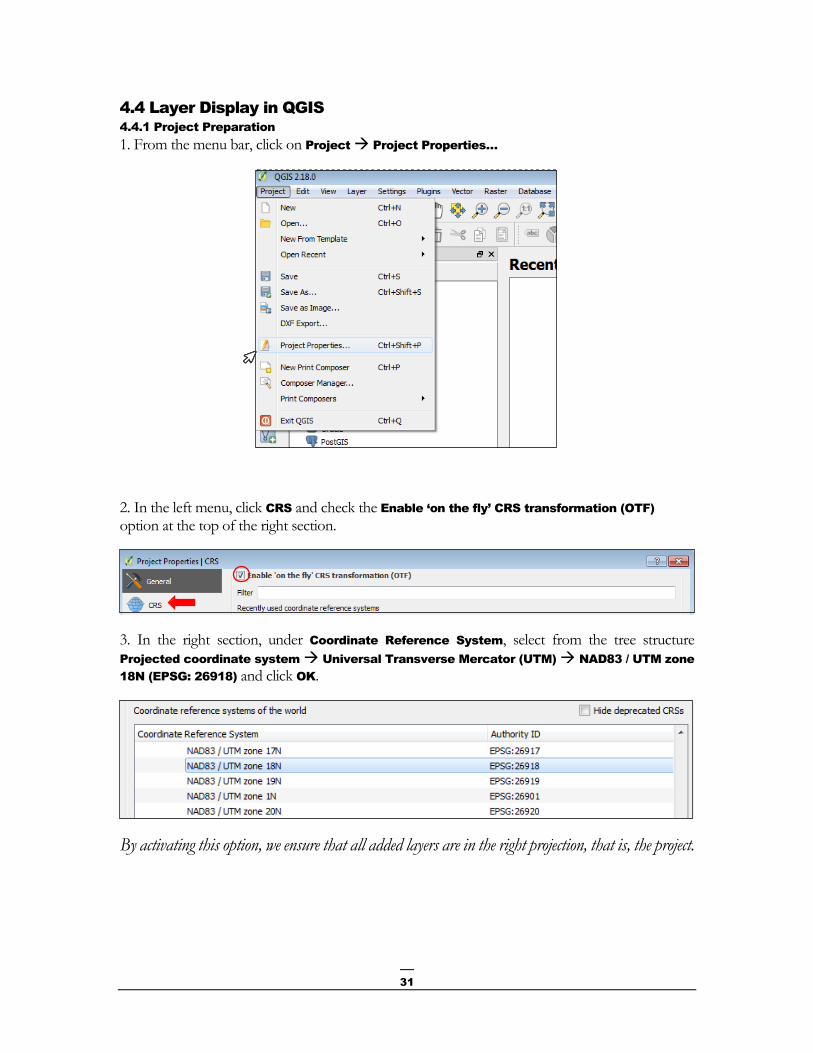
1. From the menu bar, click on Project Project Properties…
2. In the left menu, click CRS and check the Enable ‘on the fly’ CRS transformation (OTF) option at the top of the right section.
3. In the right section, under Coordinate Reference System, select from the tree structure
Projected coordinate system Universal Transverse Mercator (UTM) NAD83 / UTM zone
18N (EPSG: 26918) and click OK.
By activating this option, we ensure that all added layers are in the right projection, that is, the project.

32
4.4.2 Import Shapefiles (Form Files) and an Entity Class from a FGDB
For the demonstration we will use the following layers:
Geofiche outcrop
Diamond drilling
Regional fault
Metallic deposit
Geological zone
1:50 000 NTS sheet
1. To add data in Shapefile format, click on the button (Add Vector Layer).
2. For the Encoding field, select Latin1 (accented characters) from the drop-down menu.

33
3. In the same window, click Browse and select data of the Shapefile subsystem 32F02 from your folder. To do so:
- Select from the drop-down menu Type files, ESRI Shapefiles (*.shp *.SHP)
- Hold CRTL on the keyboard and select the desired layers.
4. Click Open to confirm the file choice.
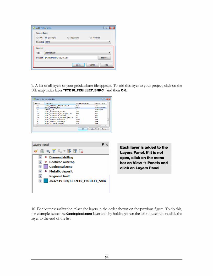
5. Click Open in the Add vector layer window to add layers to your project.
6. In extracting your data from sheet 32F02, an entity class of the 50k map index is located within
the geodatabase file. Click the (Add vector layer) button to add this layer.
7. For the Source Type, click on Directory and for the Encoding field, select Latin1 (accented characters) from the drop-down menu.
8. For the Source, click on the drop-down menu to select the OpenFileGDB Type. Note that this type of pilot does not allow you to edit the FGDB, only to consult the data. Click Browse to select your work folder and click the Open button.
34
9. A list of all layers of your geodatabase file appears. To add this layer to your project, click on the 50k map index layer “F7E10_FEUILLET_SNRC” and then OK.
10. For better visualization, place the layers in the order shown on the previous figure. To do this, for example, select the Geological zone layer and, by holding down the left mouse button, slide the layer to the end of the list.
Each layer is added to the
Layers Panel. If it is not
open, click on the menu
bar on View Panels and
click on Layers Panel

35
4.4.3 Changing the Colours of Geological Zones
To change the colour of geological zones, you can do two things:
A) QGIS Solution – Random Colours
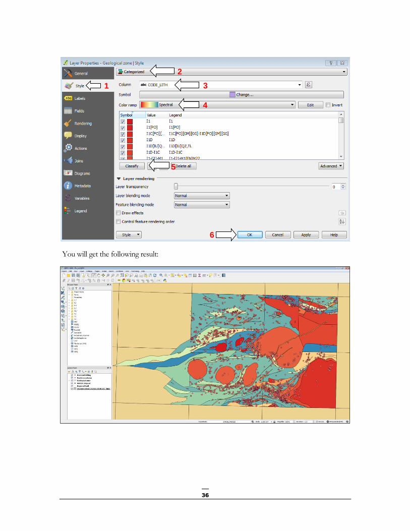
1. Double-click on the Geological zone layer (list on the left) to open the Layer Properties –
Geological zone window and click on the Style menu.
2. Choose Categorized from the first drop-down list.
3. Select CODE_LITH from the Column drop-down list.
4. Choose Spectral from the Color ramp drop-down list.
5. In the middle section, click the Classify button.
6. Click the OK button.
36
You will get the following result:
2
3
4
5
6
1

37
B) QGIS Solution – Default SIGÉOM Colours
For some information layers, it is possible to apply the different SIGÉOM colours when the “RGB” field is present in the layer. The values in this field reconstruct a colour by additive synthesis from three primary colours, red (R), green (G) and blue (B).
Beforehand, apply the SIGÉOM colours to the Geological zone layer, following these steps:
1. Double-click on the Geological zone layer (list on the left) to open the Layer Properties –
Geological zone window and click on the Style menu.
2. At the top of the window, select Single Symbol from the first drop-down list.
3. For the Symbol layer type property, click Simple fill to change the values on the right.
4. Click the icon to access the data-defined value options for filling the symbol:
4. Click on the Field type: string option and click on the RGB (string) field to associate each value in that field to the colour that will be given to the records in that layer.
5. Click the Apply button.
Your project will look like this image:

38
C) WMS Sigéom Solution (Searchable) – Palette of the Geological Map of Quebec
First, apply transparency to the Geological zone layer by following these steps:
1. Double-click on the Geological zone layer (list on the left) to open the Layer Properties –
Geological zone window and click on the Style menu.
2. At the top of the window, select Single Symbol from the first drop-down list.
3. For the Fill property, click Single fill to change the values on the right.
4. Select No brush from the Fill style drop-down list.
5. Click the OK button.
6. Repeat these steps to apply transparency to the “F7E10_FEUILLET_SNRC” layer.
Your project will look like this image:
To reference the geological map layer, with the Ministère’s official colour palette, from the WMS
SIGÉOM (searchable) service, follow these steps:
1. Click the button (Add WMS/WMTS Layer) and in the window displayed, click the New button to create a WMS connection.

39
2. In the Create a new WMS Connection window, enter the following values:
Name = “WMS SIGEOM interrogeable”
URL = http://sigeom.mines.gouv.qc.ca/SIGEOM_WMS/service.svc/get?
For more information on SIGÉOM web services, please visit http://sigeom.mines.gouv.qc.ca/signet/classes/I0000_serviceWeb
3. Click the OK button.
4. Select the “WMS SIGÉOM interrogeable” connection from the drop-down list and click the Connect button to display the list of available layers.
5. Select the data to be displayed. To do this, double-click on Geologie_Socle to display the sub-list and select “Geologie_régionale”.

40
6. Make sure that the coordinate system is the same as the project system: NAD83 / UTM zone 18N. If this is not the case, click the Change... button and select the contact system from the list.
7. Click the Add button to add the “Geologie_regionale” layer to your project.
8. Click the Close button to close the window.
9. Place the WMS layer between the Geological zone and “F7E10_FEUILLET_SNRC” layers.
41
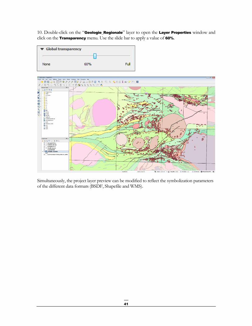
10. Double-click on the “Geologie_Regionale” layer to open the Layer Properties window and click on the Transparency menu. Use the slide bar to apply a value of 60%.
Simultaneously, the project layer preview can be modified to reflect the symbolization parameters of the different data formats (BSDF, Shapefile and WMS).

42
4.5 Display of Geophysics
There are two types of geophysical data provided by SIGÉOM (vector data):
1) Total magnetic field isovalue curves (from the Geological Survey of Canada magnetic maps). – Isovalue curve.shp
2) Punctual geophysical anomalies from the Ministère’s surveys and assessment works (input anomalies and Megatem anomalies). – Anomaly.shp
The provincial and federal WMS web services are also available to view geophysical maps in matrix format. To do this, follow these steps:
1. Click the button (Add WMS/WMTS Layer) and in the window displayed, click the New button to create a WMS connection.
2. In the Create a new WMS connection window, enter the following values:
Name = “WMS SIGEOM geophysique”
URL= http://sigeom.mines.gouv.qc.ca/ApolloCatalogWMSPublic/service.svc/get?version=1.3.0&layers=CARTE_INTERACTIVE
For more information on SIGÉOM web services, please visit http://sigeom.mines.gouv.qc.ca/signet/classes/I0000_serviceWeb
3. Click the OK button.
Federal Geophysical WMS Web Service
URL :http://wms.agg.nrcan.gc.ca/wms2/wms2.aspx?request=GetCapabilities

43
4. Select the “WMS SIGEOM geophysique” connection from the drop-down list and click the Connect button to display the list of available layers.
5. Select the data to be displayed. To do this, double-click on “Carte interactive” to display the sub-list, double-click on “Geophysique_MERN” and select “Gradient_HR”.
6. Make sure that the coordinate system is the same as the project system: NAD83 / UTM zone 18N. If this is not the case, click the Change... button and select the contact system from the list.
7. Click the Add button to integrate the Gradient_HR layer into your project and click the Close button to close the window.
44
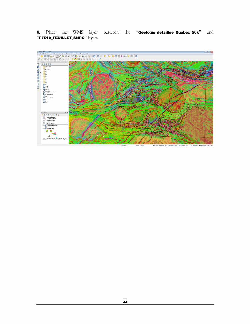
8. Place the WMS layer between the “Geologie_detaillee_Quebec_50k” and “F7E10_FEUILLET_SNRC” layers.

45
4.6 Adding Data from External Sources
4.6.1 Import a Map Background to the Project
A topographic background can be easily integrated into your project. To do this, use the “Carte de
Base du Canada (CBC)” map WMS service.
1. Uncheck the “Geologie_Regionale” and “Gradient_HR” layers.
2. Click the button (Add WMS/WMTS Layer) and in the window displayed, click the New button to create a WMS connection.
3. In the Create a new WMS connection window, enter the following values:
Name = “Carte de Base du Canada”
URL = http://geogratis.gc.ca/cartes/CBCT?
4. Click the OK button.
5. Select the “Carte de base du Canada” connection from the drop-down list and click the Connect button to display the list of available layers.
6. Select the data to be displayed. To do so, click on “CBCT”

46
7. Make sure that the coordinate system is the same as the project system: NAD83 / UTM zone 18N. If this is not the case, click the Change... button and select the contact system from the list.
8. Click the Add button to include the “Carte de base du Canada - Transport” layer in your project and click the Close button to close the window.
9. Place the layer at the end in the list of layers.
47
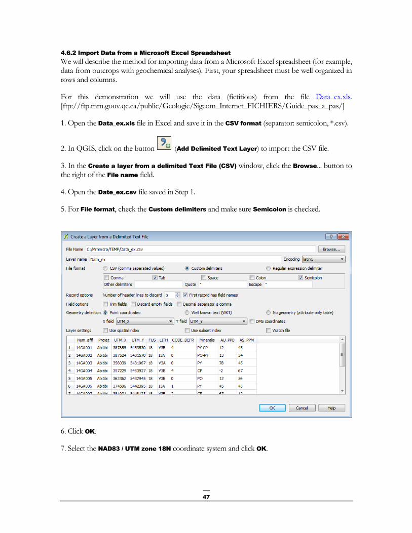
4.6.2 Import Data from a Microsoft Excel Spreadsheet
We will describe the method for importing data from a Microsoft Excel spreadsheet (for example, data from outcrops with geochemical analyses). First, your spreadsheet must be well organized in rows and columns.
For this demonstration we will use the data (fictitious) from the file Data_ex.xls. [ftp://ftp.mrn.gouv.qc.ca/public/Geologie/Sigeom_Internet_FICHIERS/Guide_pas_a_pas/]
1. Open the Data_ex.xls file in Excel and save it in the CSV format (separator: semicolon, *.csv).
2. In QGIS, click on the button (Add Delimited Text Layer) to import the CSV file.
3. In the Create a layer from a delimited Text File (CSV) window, click the Browse... button to the right of the File name field.
4. Open the Date_ex.csv file saved in Step 1.
5. For File format, check the Custom delimiters and make sure Semicolon is checked.
6. Click OK.
7. Select the NAD83 / UTM zone 18N coordinate system and click OK.

48
8. Place the Data_ex layer before the Geological zone layer in the list of layers.
9. You can change the symbol. To do this, double-click the Data_ex layer to open the Layer
Properties window and click the Style menu. Choose the symbol of your choice. For this
demonstration, the symbol being used is .
You can change the color of the other layers in order to differentiate them.

49
4.7 Relational Data Model
Not represented. Data is simplified.
4.8 Querying Data
Before doing so, add labels to the Diamond drilling layer by following these steps:
1. Double-click on the Diamond drilling layer to open the Layer Properties window and click on the Labels menu.
2. At the top, select from the first drop-down menu Show labels for this layer and select from the second drop-down menu NUMR_ORGN that represents the name of the field to be labeled.
3. Click the Color button to open the color palette and choose black.
4. Click OK.

50
Querying drilling 01-MFS-04EXT
1. Select the Diamond drilling layer.
2. Select the tool (Zoom +) to zoom into the top right corner of the project.
3. Select the tool (Identify Features) in the menu bar and click on drilling 01-MFS-04EXT.
If the item in another layer is also identified, remove this layer by unchecking its checkbox in the “Layers” tab .

51
4. The Identify Results window displays the drilling information.

52
4.9 Editing Data
QGIS allows for data editing. For example, you can add objects to a layer (e.g., drilling, outcrop, etc.). This can be done by selecting the layer to be edited from the table of contents and clicking
to toggle to Edit mode. You will then be able to add entities , move entities and more.
When you are finished, simply Save Layer Edits and Quit the update session.
4.10 Dynamic Location
Text can be freely entered in the input field and searched for a place, city, address or postal code. To do this, use the Geocoding extension installed in section 3.2 Installation.
1. From the menu bar, click on Extension GeoCoding Settings. For Geocoder engine,
select Google from the drop-down list and click OK.
2. Click on the tool (GeoCoding) and enter in the Address field: Lac Bachelor.
3. Select the NAD83 / UTM zone 18N coordinate system and click OK. The Geocoding Plugin
Results layer is added to the list of layers.
4. Change the colour of the label. To do this, double-click on the Geocoding plugin Results layer to open the Layer Properties window and click on the Labels menu. At the top, check the Show
labels for this layer option and choose black as the colour.

53
4.11 Location with Coordinates
The window can be centred on XY coordinates. To do this, use the ZoomToCoordinates extension installed in section 3.2 Installation.
1. Click on the tool (Zoom To Coordinates) and enter coordinates X: 293460 and Y: 5454639.
2. Click on (Pan to) of the tool to center the project on this coordinate.
4.12 Place a Freehand Marker
It is possible to manually place a marker somewhere in your project. To do this, use the Pin Point
extension installed in section 3.2 Installation.
1. Click on the tool (Place a Pin).
2. Choose the NAD83 / UTM zone 18N coordinate system, click OK and place your marker somewhere in your project.
3. Enter a short description and click OK. The Pins layer is added to the layers menu.
You can customize your Marker. To do this, double-click on the Pins layer to open the Layer
Properties window and click on the Labels menu. At the top, select the Label this layer with and choose the colour of your choice.

54
4.13 Sharing a Map
Does not apply.
4.14 Looking for Gold Anomalies in Drillings
Gold anomalies in drillings can be identified. Two methods are demonstrated in this guide.
4.14.1 With QGIS
We will only display drillings that contains an intermediate volcanics (V2) description and gold geochemical analysis.
1. From the list of layers, select Diamond drilling, right click and select Filter….
In the Query Builder window, it is possible to select a subset of drilling data using a SQL query. The first SELECT * FROM part of the SQL is already automatically provided to you and is not visible in the QGIS software.
For simple queries, the following general form is used:
<field_name> <operator> <value or chain>
For composite queries, the following form is used:
<field_name> <operator> <value or chain> <connector>
<field_name> <operator> <value or chain>
You can use parentheses () to define the order of operations in composite queries.
55
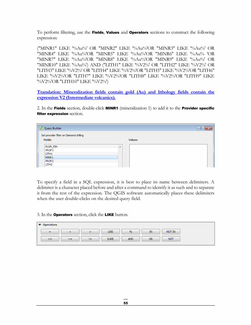
To perform filtering, use the Fields, Values and Operators sections to construct the following expression:
("MINR1" LIKE '%Au%' OR "MINR2" LIKE '%Au%'OR "MINR3" LIKE '%Au%' OR "MINR4" LIKE '%Au%'OR "MINR5" LIKE '%Au%'OR "MINR6" LIKE '%Au% 'OR "MINR7" LIKE '%Au%'OR "MINR8" LIKE '%Au%'OR "MINR9" LIKE '%Au%' OR "MINR10" LIKE '%Au%') AND ("LITH1" LIKE '%V2%' OR "LITH2" LIKE '%V2%' OR "LITH3" LIKE '%V2%' OR "LITH4" LIKE '%V2%'OR "LITH5" LIKE '%V2%'OR "LITH6" LIKE '%V2%'OR "LITH7" LIKE '%V2%'OR "LITH8" LIKE '%V2%'OR "LITH9" LIKE '%V2%'OR "LITH10" LIKE '%V2%')
Translation: Mineralization fields contain gold (Au) and lithology fields contain the expression V2 (Intermediate volcanics).
2. In the Fields section, double-click MINR1 (mineralization 1) to add it to the Provider specific
filter expression section.
To specify a field in a SQL expression, it is best to place its name between delimiters. A delimiter is a character placed before and after a command to identify it as such and to separate it from the rest of the expression. The QGIS software automatically places these delimiters when the user double-clicks on the desired query field.
3. In the Operators section, click the LIKE button.

56
Here are the possible operators to use when filtering SQL in QGIS:
Yellow: Generic characters used to search by partial string
Red: comparison operators
Green: logical operators
Operator Description
= x Selects a record if it has a value equal to x for the specified attribute.
< x Selects a record if it has a value less than x for the specified attribute.
<= x Selects a record if it has a value less than or equal to x for the specified attribute.
> x Selects a record if it has a value greater than x for the specified attribute.
>= x Selects a record if it has a value greater than or equal to x for the specified attribute.
!= x Selects a record if it has a different value of x for the specified attribute. This is equivalent to the following operators: NOT =
IN (x, y, z) Selects a record if it contains an element in a field from several chains or values (x, y or z).
LIKE
To search using a partial string, use the LIKE operator and add generic characters. The percentage symbol (%) means that it can be replaced by anything: one character, a hundred characters or no characters. However, to perform a search with a generic character representing a single character, use the underscore character (_). LIKE works with character-type data on both sides of the expression. * Operator of this query *
ILIKE Unlike LIKE, chain correspondence is case-insensitive.
% Represents zero, one or more characters that are not part of the partial chain
when using the LIKE or ILIKE operator. * Operator of this query *
NOT Selects a record if it does not match the expression.

57
AND Combines two conditions together and selects a record if both conditions are true.
OR Combines two conditions together and selects a record if at least one
condition is true. * Operator of this query * NOT IN
Selects a record that has no value.
4. In the Provider specific filter expression section, enter, following the LIKE, ‘%Au%’. Thus, the display filter will be on items that contain this part of the text as a value.
5. In the Operators section, click the OR button.
6. Repeat steps 1 to 6 for MINR2, MINR3 fields up to MINR10.
7. Put the mineralization expression in parentheses.
8. In the Operators section, click the AND button.
9. In the Fields section, double-click LITH1 (lithology 1) to add it to the Provider specific filter
expression section.
10. In the Operators section, click the LIKE button.
11. In the Provider specific filter expression section, enter, following the LIKE, ‘%V2%’.
12. In the Operators section, click the OR button.
13. Repeat steps 10 to 13 for LITH2, LITH 3 fields, up to LITH 10.

58
14. Put the second part of the expression on the lithologies in parentheses.
15. Click OK.
16. To validate the result of your query, right click on the Diamond drilling layer and then click on Open Attribute Table. The number of entities filtered based on your query is displayed in the attribute table dialogue box header:
If you want to see the total number of entities in your layer without filtering, you must open the Filter tool again, delete the entered query and click OK. Note the total number of entities without filters in the column header of the attribute table dialogue box.
Note:
Shapefile geometric data is always associated with a dbf file that contains descriptive information. The dbf format has several limitations, including the total number and length of fields, as well as a limit on the total volume of data. In order to integrate the SIGÉOM data into this data format, a de-normalization of the relational model of the data was performed to present it in the form of a single table instead of several linked tables as is the case in a relational model. Some descriptive information from several tables in the relational model is used to complete a single table in the Shapefile data format.
This has an impact on the ability to make requests, in particular to select drillings with a certain content. The following example comes from a drilling with several intersections.
The search for drillings with a gold content greater than 1000 ppb is not possible since it is a text field. We propose the following method for dealing with this limitation.

59
4.14.2 With SIGÉOM à la carte
A drilling KML file containing a description of intermediate volcanics (V2) and geochemical analysis exceeding a threshold of 1000 ppb (1 g/t) gold can be obtained by SIGÉOM à la carte.
1. On the SIGÉOM à la carte homepage, click on Drilling to be directed to its entities and descriptions. Then click on the Diamond drilling entity.
2. Enter the following values in the appropriate fields.
3. Click the button on the left menu to run the query.
4. Quelques secondes s’écouleront afin que le fichier KML soit disponible pour son téléchargement. Cliquez ensuite sur le bouton « Télécharger le KML » :
85
60
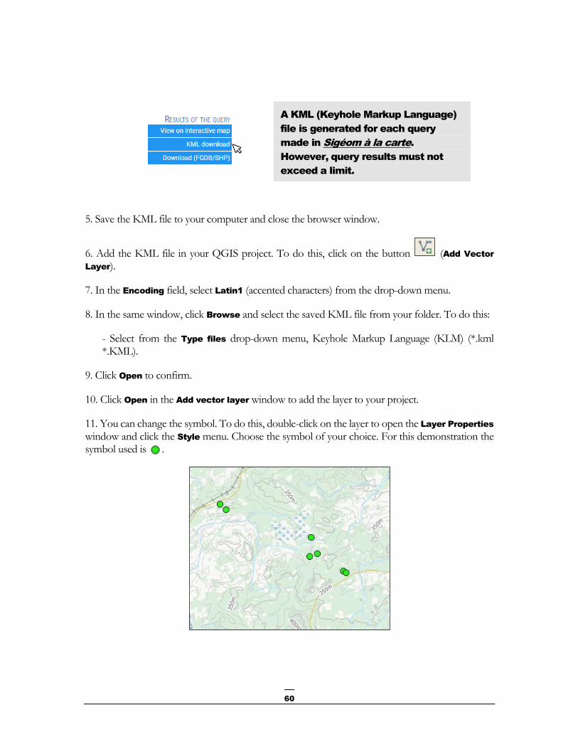
5. Save the KML file to your computer and close the browser window.
6. Add the KML file in your QGIS project. To do this, click on the button (Add Vector
Layer).
7. In the Encoding field, select Latin1 (accented characters) from the drop-down menu.
8. In the same window, click Browse and select the saved KML file from your folder. To do this:
- Select from the Type files drop-down menu, Keyhole Markup Language (KLM) (*.kml *.KML).
9. Click Open to confirm.
10. Click Open in the Add vector layer window to add the layer to your project.
11. You can change the symbol. To do this, double-click on the layer to open the Layer Properties window and click the Style menu. Choose the symbol of your choice. For this demonstration the symbol used is .
A KML (Keyhole Markup Language)
file is generated for each query
made in Sigéom à la carte.
However, query results must not
exceed a limit.
61
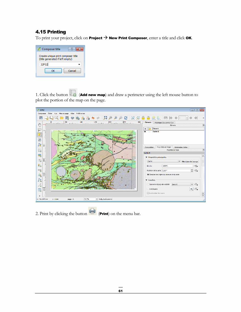
4.15 Printing
To print your project, click on Project New Print Composer, enter a title and click OK.
1. Click the button (Add new map) and draw a perimeter using the left mouse button to plot the portion of the map on the page.
2. Print by clicking the button (Print) on the menu bar.

62
5. ESRI FGDB Format
In this example, we use the ArcGIS 10 software from ESRI.
5.1 Cost
Paid use. Refer to ESRI Canada website: https://www.esri.ca/fr.
5.2 Access to Data
You can access geoscientific data via the SIGÉOM home page. You must follow the steps outlined in Section 4.3 Access to Data to download the Atlas data in FGDB and Shapefile.
Following your order, you will receive a secure email to download your data.
Then, by opening the .MXD file (example: 1017030-REQT1.MXD), geological data should be displayed with the specific symbolization of each entity type. Note that a .MXD file exists for each data types, FGDB and Shapefile.
5.3 Layer Display
After opening the .MXD, all the layers of the FGDB will be displayed in the ArcMap session and in the Table of Contents list. If the table of contents is not visible, click on Windows in the pop-up menu and then Table of Contents. You can then turn on or off the layers of your choice.
Hold the CRTL key down and uncheck the first layer of the table of contents. All layers will now be turned off. Then check only the following layers: Diamond drilling, Mineralized body, Geofiche outcrops, Geological contact, Regional fault and Geological zone. Then right click on the Geological zone layer and click Zoom to layer. You should have on screen an image similar to the following figure:
To apply transparency to a layer, go to the layer’s property (right click on the layer – Properties…). Then, under the Display tab, apply the desired transparency percentage.

63
5.4 Display of Geophysics
There are two types of geophysical data provided in SIGÉOM FGDB (vector data):
1) Total magnetic field iso value curves (from the Geological Survey of Canada’s magnetic maps).
2) Punctual geophysical anomalies from the Ministère's surveys and assessment works (input anomalies and Megatem anomalies).
However, it is also possible to access the provincial and federal WMS servers to display geophysical maps in matrix format. To do this, you must open the ArcCatalog utility and open the GIS
Server tab in the Location window.
Then double-click on the Add WMS Server tab and the following window appears:
64
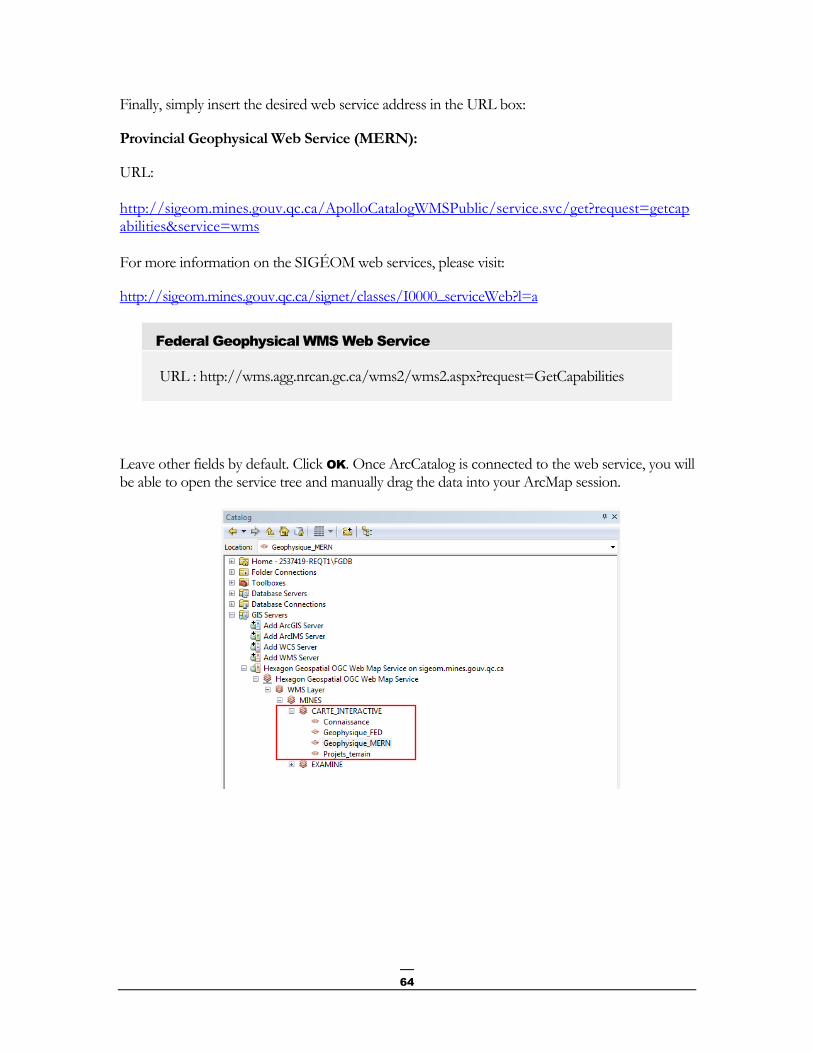
Finally, simply insert the desired web service address in the URL box:
Provincial Geophysical Web Service (MERN):
URL: http://sigeom.mines.gouv.qc.ca/ApolloCatalogWMSPublic/service.svc/get?request=getcapabilities&service=wms
For more information on the SIGÉOM web services, please visit:
http://sigeom.mines.gouv.qc.ca/signet/classes/I0000_serviceWeb?l=a
Federal Geophysical WMS Web Service
URL : http://wms.agg.nrcan.gc.ca/wms2/wms2.aspx?request=GetCapabilities
Leave other fields by default. Click OK. Once ArcCatalog is connected to the web service, you will be able to open the service tree and manually drag the data into your ArcMap session.

65
5.5 Adding Data from External Sources
To add data from external sources, simply use the Add Data button: .
One can thus include a variety of file types, such as Shapefile, entity classes, rasters, images, Microsoft Excel spreadsheets, Microsoft Access databases, text files (txt), etc.
Import a map background to the ArcMap project:
To import a map background to the project, click the black arrow to the right of the Add Data button and click Add Basemap.
You can then add imagery, streets, topography, etc.
Click on the desired map background and click Add. Next, you can apply transparency to your Geological zone layer:

66
5.6 Import Data from a Microsoft Excel Spreadsheet
We will detail how to import data from a Microsoft Excel spreadsheet (for example, outcrop data with geochemical analyses). First, your spreadsheet must be well organized in rows and columns. Click on File – Add data and Add XY data.
Then navigate to the Excel file in question by clicking on the button with the small yellow folder.
If your table contains multiple
sheets, you must specify which
one contains data to import into
your project.

67
Select Sheet 1 and click Add.
Afterwards, you must specify which column of your spreadsheet contains the X coordinates (X
Field) and which contains the Y coordinates (Y Field). Then you have to specify to the software what geographic projection it is. To do so, click Edit... and select the correct projection from the Spatial Reference Properties window.
Click OK and also click OK in the Add XY data window.
The selected sheet now appears in the table of contents (e.g. Événements Feuil1$) and corresponding points on the map.
To export the file to a Form file or geodatabase, right click on the layer, click on Data and Export
Data… .

68
Click the button with the yellow folder to select the directory where you want to save your geodatabase file. Then you will have the option to save your file as a Form file or entity class (for a geodatabase).

69
5.7 Relational Data Model
SIGÉOM data relational models are illustrated in PDF documents which are provided when ordering data from “SIGÉOM à la carte”. A PDF document is available for each entity. As an example, we will be detailing here the Diamond drilling entity to better understand the data structure.
The entity class (green) contains basic diamond drilling information such as azimuth, dip, coordinates, altitude, year, source, comment, etc.
The linked tables contain detailed information on lithology. As drilling can contain several lithological types, the information is contained in separate tables. Each lithology is associated with a drilling by a unique number.
Feature class
Connected table

70
In addition, the PDF document of the relational model provides, where applicable, the value domains including the specific description of each value:
In the example above, values in the “CODE_PREC_LOCL” field must contain one of the values displayed in the list. For each of these values, it is possible to see their description (the assignment).

71
5.8 Querying Data
Here are three simple ways to query data in the ArcGIS environment: by using the Identify button, by looking at the entity class tables and by using SQL queries.
1) By using the Identify button:
You can query data directly using the Identify button: .
By clicking on the object, a window appears with the object information contained in the entity class or form file table.
You can view the information in the linked tables by clicking on the + on the left of the drill number.
This will allow you to view the tables containing lithological information (F5E05_UNITE_LITHOLOGIQUE) and mineralization information (F5E06_SEQUENCE_MINERALISATION).

72
SIGÉOM
Fields
column
Layer
informations
column

73
Information on the field definition can be found in the SIGÉOM field glossary at:
http://sigeom.mines.gouv.qc.ca/signet/classes/I3202_glosElmnDonn?l=a
2) By consulting the entity class tables:
For each layer, you can also consult the entity class table and linked tables associated with that layer. To do this, right click on the Open Attribute Table layer. All layer information is then displayed. You can also access the linked table information by clicking on the Related Tables button .
By clicking on the link below the button, you can access the table containing lithological information (F5E05_UNITE_LITHOLOGIQUE).

74
Once in table F5E05_UNITE_LITHOLOGICAL, you have the option to display table F5E06_SEQUENCE_MINERALISATION by clicking on the Related Tables button or you can return to the original drilling table.
3) Using SQL queries :
It is also possible to query data using SQL queries. Click Selection from the pop-up menu and Select by attribute…
. The following window will appear:
The SQL query operation in ArcMap is similar to that of QGIS (Section 4.14).
First, you must choose which entity you want to query using the Layer drop-down menu. Then, at the bottom of the window, in the white field, you can query data using SQL operators such as LIKE, AND, OR, =, +, -, etc.
The Select by attribute tool interface from the Selection menu:
The SQL query operation in ArcMap is
similar to that of QGIS
<field name> <operator> <value or chain>
Select the target layer, i.e. the layer you want to select from.
You can limit the list of target layers to only selectable layers, but by default, all layers are available.
You can choose the type of selection to be made based on your needs:
List of fields in the target layer; double-click on a field to insert it into the query expression.
List of unique values of the selected field; double-click on a value to insert it into the query expression.
Key operator dial; click once on an operator to insert into the query expression.
Click the Get Unique Values button to view the selected field's values when creating an expression.
Compose a query expression using the following methods:
Create a query using expression creation tools;
ompose a query in the selection window;
Load a record.

75
The Select by attribute tool interface from the Table:
You can check the validity of the expression at any time.
You can choose the type of selection to be made based on your needs:
List of fields in the target layer; double-click on a field to insert it into the query expression.
List of unique values of the selected field; double-click on a value to insert it into the query expression..
Key operator dial; click once on an operator to insert into the query expression.
Click the Get Unique Values button to view the selected field's values when creating an expression.
Compose a query expression using the following methods:
Create a query using expression creation tools;
ompose a query in the selection window;
Load a record.

76
The possible results are: An error was detected in the expression. SQL instruction used is not valid...
There is a syntax error in the request expression.
The expression was successfully processed but no records were found.
There are no errors in the expression syntax, but no record meets the criteria and will therefore not be selected.
The expression was successfully processed.
There are no errors in the expression syntax and at least one record meets the criteria and will be selected.
REC ORD A ND LOA D A QU ERY EX PRE SS IO N
You can save and reload selection expressions using the Save and Load buttons at the bottom of the Apply tool. This option allows you to quickly recreate a selected set of records by loading a saved expression.
The format of an expression recorded using ArcMap is .EXP.
Examples of queries (in the Diamond drilling layer):
1) "NUMR_ORGN_FORG" = '01-MFS-04EXT'
Translation: The original Drilling number is equal to 01-MFS-04EXT.
2) "NUMR_ORGN_FORG" LIKE '%MFS%'
Translation: The original Drilling number contains the term “MFS”.
3) "AN_FORG" > 2003 AND "NUMR_RAPR" = 'GM 66733'
Translation: The drilling's year of publication is greater than 2003 and the drilling comes from the Examine GM 66733 report.

77
5.9 Data Editing
Unlike the interactive map and server, WMS and ArcGIS allow data editing. You can add objects (e.g., drilling, outcrop, etc.), remove objects or modify objects (e.g., geological polygons). To do this, the editing bar must be added. Simply right-click in a grey space above the data page and add the Editor toolbar. Then click the Editor button and Start Editing.
To create or add objects, simply click on the Create Features button from the toolbar, select the entity to be added/edited from the Create Features window and plot/add the object directly to the map. When you are finished, simply Save Edits (under Editor) and Stop Editing.
78
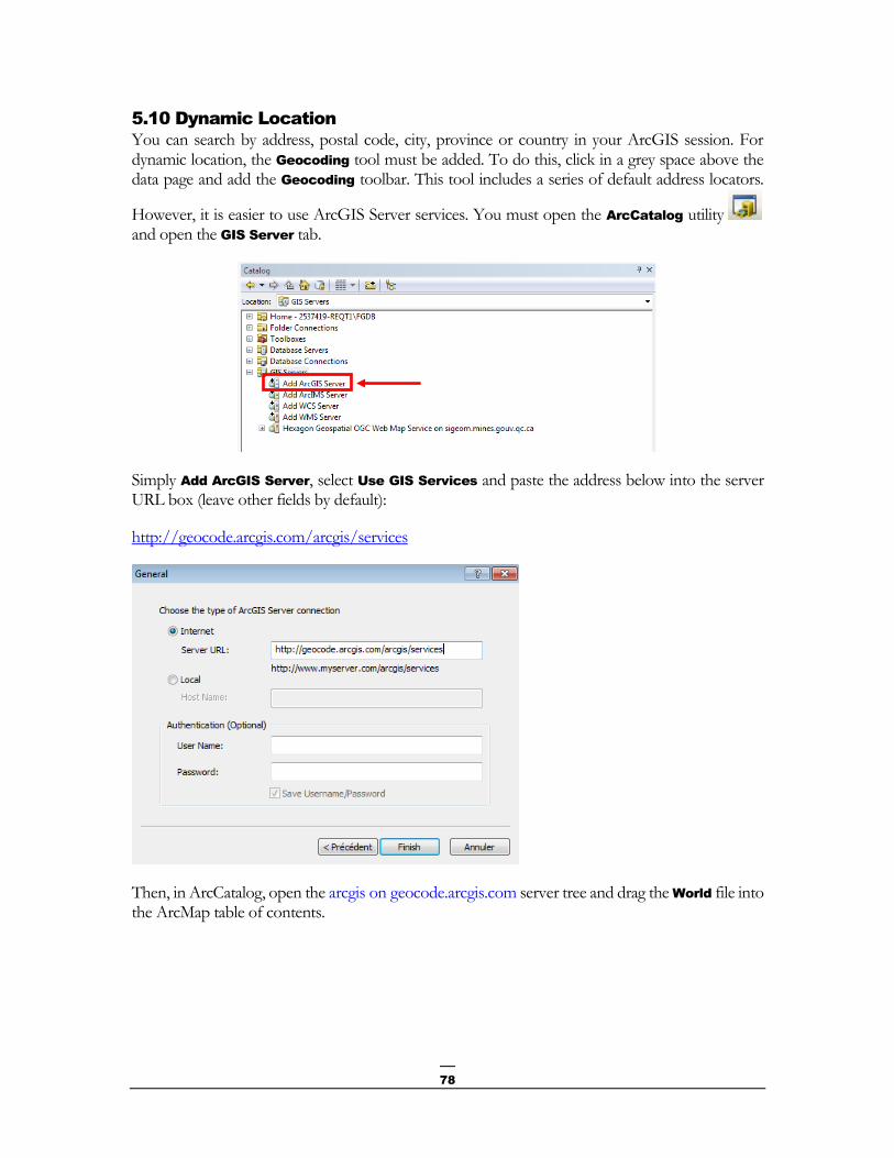
5.10 Dynamic Location
You can search by address, postal code, city, province or country in your ArcGIS session. For dynamic location, the Geocoding tool must be added. To do this, click in a grey space above the data page and add the Geocoding toolbar. This tool includes a series of default address locators.
However, it is easier to use ArcGIS Server services. You must open the ArcCatalog utility and open the GIS Server tab.
Simply Add ArcGIS Server, select Use GIS Services and paste the address below into the server URL box (leave other fields by default):
http://geocode.arcgis.com/arcgis/services
Then, in ArcCatalog, open the arcgis on geocode.arcgis.com server tree and drag the World file into the ArcMap table of contents.

79
Then, simply select World from the Geocoding tool and enter the desired address:
Then, with a right click on the address, you have the option to create the point, locate the address on the map (Zoom To) or add a geomarker to that location.

80
5.11 Location with Coordinates
You can search by coordinates by clicking on the tool Go to XY . This tool allows you to enter coordinates to locate a point on the map. You must select the unit Meters to enter UTM coordinates.
There is also a dynamic locator at the bottom right of the screen. Coordinates for your mouse pointer is provided. To change the locator view, simply click on Display – Data block properties
– General – Units. You will then be able to select the unit of your choice.

81
5.12 Sharing a Map
In the ArcGIS environment, there are different ways to export and share a map:
1) You can export your map in a georeferenced image format. This way, other users will be able to view your map in the AcrGIS environment, but will not be able to edit it (this is an image file). To do this, you must click on the File and Export Map… menu. Next, you will need to select the file type and Save. Your map is then saved in a georeferenced image format.
2) You can send all of your data (GDF, Shapefile, etc.) with a MXD file. However, by sharing your map this way, you run the risk of forgetting data or files. In addition, other users will only be able to open your ArcMap project if they use the same version of ArcGIS as you (or a newer version). Map Package are preferred (option #3).
3) You can create a Map Package. To do so, click on File from the pop-up menu and Share As and Map Package… .
Then, in the Map package window, click Save package to file and indicate where to save this file to your station. You must also check Include company geodatabase data instead of referencing
the data.

82
Then, you must open the Item Description tab in the left menu.
Item description fields (abstract, tags and description) are mandatory fields to create the map package. Check the Update missing metadata option. You can add Additional files (if any) with the package.

83
You can then click on the Share button at the top right. The layer package is then exported to your station. This is an MPK extension file, a zipped file format. You can now send this package to other users.
To open a layer package (MPK file), you must use the Extract a package tool.
To do this, click ArcToolbox and open the Data management tools toolbox. In this box, open the Package toolset and finally the Extract package tool. The following window will appear:
Indicate in the Input package space where the MPK compressed file is located on your station and in the Output Folder where you want to extract the data. Click OK. You will find the MXD file and the geodatabase in the Output Folder.

84
5.13 Looking for Gold Anomalies in Drillings
The ArcGIS environment allows for much more specific and detailed queries than the interactive map and QGIS freeware.
Here we will detail an example of a SIGÉOM data query to better understand the relational model of these data. First, we will identify drillings that are within 100 metres of a regional fault or shear zone. Of these, we will then select those that contain an intermediate volcanic (V2) description whose geochemical analysis exceeded a 1000 ppb (1 g/t) gold threshold.
Method:
1) First, you must select drillings within 100 metres of a regional fault or shear zone. To do this, in the Selection menu, click Select by location. In the window that appears, you must select the selection method by selecting select feature from and select Diamond drilling as the target layer (this is the layer you want to select from). Then select Regional fault as the source layer. For the spatial selection method, you must select Target layer(s) features intersect the Source layer
feature. The search distance here will be 100 metres. Click OK. Drillings within 100 metres of a regional fault or shear zone are now selected.

85
The Select By Location tool allows you to select entities based on their relative position in another layer.
About selection methods
You can choose the type of selection to be made based on your needs:
Select target layer(s) from which entities will be selected – you understand this, you can perform a spatial selection over multiple layers at the same time.
You can limit the list of target layers to only selectable layers, but by default, all layers are available.
Select the source layer to be used to select entities in the target layer. For example, if you want to select diamond drillings that cut regional faults, the target layer would be diamond drillings and the source layer would be regional faults.
You can use all the entities in the source layer or only the
previously selected entities . Select the selection method (spatial relationship rule) to use for selection.
You can also use a search distance, i.e. extend the reference surface of your source layer by a certain distance (buffer zone, tolerance).
The proposed spatial selection methods depend on the type of data (points, lines, polygons) in the target layer and source layer. The Search distance option is available only with certain selection methods. All methods can be found in Appendix 1 of this document.

86
2) From drillings selected in Step 1, you must now find drillings that contain an intermediate volcanic (V2) description. To do this, you must open the Diamond drilling layer attribute table and go to the linked table: Lithological unit. In the attribute table, click once on the Related Tables button to go to table F5E05_UNITE_LITHOLOGIQUE. Once in the table, to select V2 lithologies, you must click on Table Options and Select By Attribute.
For the selection method, choose Select from current selection because you want to select only from the entities already selected (within 100 m of a fault). Now write this query in the white space at the bottom of the window:
"LITH" LIKE '%V2%'
Meaning: The lithology column contains the expression V2 (Intermediate volcanics).
Click Apply.
3) From drillings selected in Steps 1 and 2, you must now find drillings that contain >1000 ppb of gold (1 g/t). To do this you have to go to the linked table Mineralization sequence. Click once on the Relateded Tables button to go to table F5E06_SEQUENCE_MINERALISATION. Once in the table, to select gold levels above 1000 ppb, you must click on Table Options and select by attributes.

87
For the selection method, choose Select from current selection because you want to select only from entities already selected (within 100 m of a fault and containing V2 lithology). Now write this query in the white space at the bottom of the window:
"CODE_ELMN_CHIM" = 'Au' AND "TENR" >= 1000
Meaning: Chemical element equals Gold and content is greater or equal to 1000.
Click Apply and Close the window.
Drillings located less than 100 metres from a fault or shear zone and that contain an intermediate volcanic (V2) description, whose geochemical analysis exceeded a threshold of 1000 ppb of gold, are now selected.

88
5.14 Printing
To print a map, it is best to put ArcMap into Layout mode. To add a legend, the ArcMap session must be formatted (View – Layout View). Then, under the Insert tab, you can add a legend, north arrow, scale bar, etc. In Layout mode, you can also adjust the scale of the map.
Once the layout is complete, click on File – Page and Print Setup.
The Page and Print Setup window allows you to select the printer, print area size (Paper) and map size. Once the layout is complete, click File – Print to start printing. You can also install a PDF utility (e.g., PDFCreator) to create a PDF file.
89
5.15 Difference Between Shapefile and FGDB
A shapefile is a simplified format for storing vector data to archive the location, shape and attributes of geographic features. It can only contain point, linear (line) or surface (polygon) entities. A shapefile is very limited in terms of file size (2 GB), the number of objects it can contain and the number of possible fields. A geodatabase is a package of files in a folder that allow to store, query and manage spatial and non-spatial data. It stores many types of objects (entity classes, many raster types, images, tables, etc.). Geodatabases are used to process and manipulate very large data sets.
Geological data from SIGÉOM are stored in a geodatabase.
There are two types of geodatabase:
The personal geodatabase (MDB) is based on a Microsoft Access structure. It is limited in size (based on the Windows operating system version), but allows for the transfer of Microsoft Office data (Excel, Access). In addition, MDB can also be used to process lithochemical data from other software (e.g. GCD kit, Lithomodeleur, Geointerpreter, etc.). It is only used on Windows platforms.

90
The file geodatabase is based on an ArcGIS structure. It is virtually unlimited in size (1 TB). This limit can be as high as 256 TB for large image sets. Each entity class in a FGDB can contain more than 2 billion vector entities per dataset. The FGDB is a unique tool that allows for optimal organization of data. It allows a multitude of files to be grouped into a single database (one file). It can be used on multiple platforms. This type of geodatabase uses about one third of the storage space for the same information with respect to personal geodatabases or shapefiles. To create a shapefile, a personal geodatabase or a file geodatabase file, you must open the ArcCatalog utility and navigate to the folder of your choice. Then right click on the folder and select New.

91
Conclusion
We have shown you how to access, analyze and edit SIGÉOM data using three technologies that use different formats. Our objective was to guide you so that you could use Quebec geoscientific data managed by the Ministère.
Highlights related to each technology are:
1. Interactive map: The map allows different geoscientific layers to be viewed using Internet Explorer, Firefox or Google Chrome. Active and in-demand mining titles linked to the GESTIM system are also available. The interactive map is free of charge and we receive about 30 000 visits a year. This approach is aimed at the general public and geoscientists. The interactive map has been available since late 2012.
2. Web Map Service (WMS) informatics service: The service provides the ability to
display SIGÉOM geoscientific information layers. This service can be used with freeware such as QGIS – which is used in this guide – or other software such as MapInfo (used by several exploration companies). Use of the WMS service is free of charge. This approach is aimed at a clientele with more specific consultation needs (mining exploration, academia, government departments, etc.). WMS service has been available since 2012.
3. File Geodatabase (FGDB) data: It is a format that can be exploited in the ArcGIS
environment or with other software. Data are sold to the customer. This format allows analysis and modelling of SIGÉOM data by applying filters and selecting and discriminating the information they want to process. Because data format is more complex, prior knowledge is required to exploit it. This format has been available since 2010.
The following table provides a summary of the functions that were exploited during the demonstrations. The major differences between the interactive map environment and QGIS are that the interactive map data model is simplified and the addition of external data – including WMS services – is not possible. In terms of the differences between ArcGIS and QGIS, there are many. ArcGIS is a sophisticated software program that allows the entire SIGÉOM geometric and descriptive data model to be used at home. It requires a significant financial investment for its acquisition and for user training. Before acquiring ArcGIS, we have to realize that we will find ourselves in an environment designed by geomatics specialists for geomatics users. For QGIS, it’s a freeware that never ceases to amaze us. This version announces the possibility of opening a FGDB. The software has faults in its qualities, like all open source software that requires a fair amount of user resourcefulness.

92
In conclusion:
Free consultation of SIGÉOM data - Interactive map;
Pooling of SIGÉOM data, other data sources and ours - QGIS and others via the SIGÉOM WMS service.
Editing, data relational model and sophisticated spatial data queries - ArcGIS.
Comparison Table
Different Work Environments
Demonstration Object MAP QGIS ARCGIS
Layer display (drilling, geology, outcrop, deposit and fault)
Display of geophysics
Adding data from external sources
Querying data
Data editing
Dynamic location
Location with coordinates
Placing a freehand marker
Map sharing with web link
Looking for gold anomalies in drillings
Data relational model
Difference between shapeFile and FGDB
Printing

93
Contact us
If you have any questions or comments, please do not hesitate to contact us.
Email: [email protected]
Mines Service Centre
Telephone: (418) 627-6278
Toll-free line: 1-800-363-7233
Fax: (418) 643-2816
94
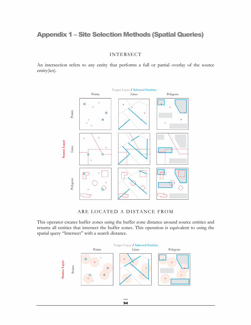
Appendix 1 – Site Selection Methods (Spatial Queries)
IN TERSEC T
An intersection refers to any entity that performs a full or partial overlay of the source entity(ies).
Target Layer / Selected Entities Points Lines Polygons
So
urc
e L
ayer
Po
ints
Lin
es
Po
lygo
ns
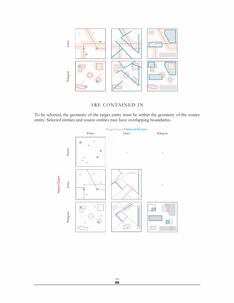
ARE LOC A TED A D I S TA NCE FR O M
This operator creates buffer zones using the buffer zone distance around source entities and returns all entities that intersect the buffer zones. This operation is equivalent to using the spatial query “Intersect” with a search distance.
Target Layer / Selected Entities Points Lines Polygons
So
urc
e L
ayer
Po
ints
95
Lin
es
Po
lygo
ns
ARE C ON TA INE D I N
To be selected, the geometry of the target entity must be within the geometry of the source entity. Selected entities and source entities may have overlapping boundaries.
Target Layer / Selected Entities Points Lines Polygons
So
urc
e L
ayer
Po
ints
-- --
Lin
es
--
Po
lygo
ns

96
ARE C OM P LE TE LY CO N TA INED IN
To be selected, all parts of target entities must be within the source entity(ies) geometry and cannot touch the source boundary. The source entity must be a polygon, where you must apply a buffer zone around point and linear entities to use that operator. This operator is the reverse of "Contain completely".
Target Layer / Selected Entities Points Lines Polygons
So
urc
e L
ayer
Po
ints
-- -- --
Lin
es
-- -- --
Po
lygo
ns
C ON TA IN
To be selected, the geometry of the source entity must be within the geometry of the target entity that includes its boundaries. This is the reverse of the operator “Are in”.
Target Layer / Selected Entities Points Lines Polygons
So
urc
e L
ayer
Po
ints
Lin
es
--

97
Po
lygo
ns
-- --
C ON TA IN CO M P LE TE LY
To be selected, all parts of the target entity must contain the complete geometry of the source entity. In addition, the source entity cannot touch or superimpose on the boundaries of the target. The source entity must be a polygon, where you must apply a buffer zone around point and linear entities to use that operator.
Target Layer / Selected Entities Points Lines Polygons
So
urc
e L
ayer
Po
ints
-- --
Lin
es
-- --
Po
lygo
ns
-- --

98
H AVE THE IR CENTR O ID IN
A target entity is selected by that operator if the centroid of its geometry is in the geometry of the source entity or its boudaries.
Target Layer / Selected Entities Points Lines Polygons
So
urc
e L
ayer
Po
ints
Lin
es
Po
lygo
ns
S HARE A L INE SEG M EN T W ITH
With this method, source and target entities are considered to share a line segment if their geometries share at least two contiguous apexes in common. The source and target entities must be lines or polygons.
Target Layer / Selected Entities Points Lines Polygons
So
urc
e L
ayer
Po
ints
-- -- --
Lin
es
--

99
Po
lygo
ns
--
ARE BOR DER ING TH E L IM IT OF
A target entity is selected if the intersection of its geometry with the source entity geometry is not empty while the intersection of their interiors is empty. This is the definition of the touch operator Clementini. Therefore, if the target entity touches the source entity, it is selected. Clementini indicates that the limit of a polygon is distinct from its interior and exterior. The source and target entities must be lines or polygons. An additional case is also supported - an inner line or polygon wholly contained in a polygon is selected if its geometry shares segments of line, apexes or ends with the polygon boundary.
Target Layer / Selected Entities
Points Lines Polygons
So
urc
e L
ayer
Po
ints
-- -- --
Lin
es
--
Po
lygo
ns
--

100
ARE ID EN TICA L TO
Two entities are considered identical if their geometries are strictly equal. Entity types must be the same.
Target Layer / Selected Entities Points Lines Polygons
So
urc
e L
ayer
Po
ints
-- --
Lin
es
--
--
Po
lygo
ns
--
--
ARE CR OSSE D BY THE C O N TOUR OF
With this operator, the boundary of the source and target entities must have at least one common segment, apex or end, but must not share a line segment. The source and target entities must be lines or polygons.
Target Layer / Selected Entities Points Lines Polygons
So
urc
e L
ayer
Po
ints
-- -- --
Lin
es
--

101
Po
lygo
ns
--
C ON TA I N (C LE ME N TIN I )
This operator gives the same results as the operator Contain unless the source entity is entirely located on the target entity boundary and no part of the source entity is within the target entity. In this case, the operator Contain (Clementini) does not select the target entity, unlike the operator Contain. Clementini indicates that the polygon boundary is distinct from its interior and exterior.
Target Layer / Selected Entities Points Lines Polygons
So
urc
e L
ayer
Po
ints
Lin
es
--
Po
lygo
ns
-- --

102
ARE C ON TA INE D I N (C LE ME N TIN I)
This operator provides the same results as the operator “Are contained in” unless the target entity is entirely located on the source entity boundary and no part of the target entity is within the source entity. In this case, the operator Are contained in (Clementini) does not select the target entity, unlike the operator Are contained in. Clementini indicates that the polygon boundary is distinct from its interior and exterior.
Target Layer / Selected Entities Points Lines Polygons
So
urc
e L
ayer
Po
ints
Lin
es
Po
lygo
ns

103
Appendix 2 – Data and Coordinate System
Data extracted from SIGÉOM in “SHAPEFILE” and “FGDB” format are recorded in geographic coordinates in the geodetic reference system NAD83 based on the GRS80 ellipsoid. It is possible to change the coordinate system at the data source or only when viewing the data in a GIS. This annex outlines the different ways in which this can be achieved using ArcGIS and QGIS GIS software.
ArcGIS Software
Change the coordinate system at the source
1st solution:
In ArcCatalog, double-click on the appropriate Shapefile or entity class (FGDB) to access the properties. On the XY Coordinate System tab, click the Select... button. If you want to project your data into Modified Transverse Mercator (MTM), Universal Transverse Mercator (UTM) or Lambert concordant conic projection, then click on Projected Coordinate Systems \ National
Grids \ Canada and select the desired coordinate system.
2nd solution :
Using ArcToolbox’s Data Management Tools\Projections and
Transformations\Feature\Project, set up the tool with the desired coordinate system:

104
Change the coordinate system for viewing
When your data are displayed in ArcMap, it is possible to change the coordinate system only to view it without changing the system at the source. To do this, the coordinate system must be modified in the properties of the data block. Double-click on the data block to access properties. In the Coordinate system tab, click Modify… and project your data only into the ArcMap view by selecting the desired coordinate system.
QGIS Software
Change the coordinate system for viewing
Overall specification of a project coordinate system:
The coordinate system for a QGIS project can be changed in its properties. It can be accessed through the Project menu and then clicking on Project properties… or simply by clicking on the button at the bottom right of the software interface. Once in the Project properties, the Enable “on the fly” CRS transformation (OTF) checkbox must be activated, and it is possible, afterwards, to access the different coordinate systems for the change.
Coordinate system specification for a layer:
The coordinate system of a layer found in a QGIS project can be changed in its properties. It can be accessed by right-clicking on the layer and clicking on Properties or double-clicking on the layer. In the General tab of the layer properties and in the Coordinate Reference System section, click on the button to open the Coordinate Reference System Selector window. If you wish to project your data into Modified Transverse Mercator (MTM), Universal Transverse Mercator (UTM) or Lambert Concordant Conic Projection, select the desired system under Projected
Coordinate systems (1) of the Coordinate Reference System section. Also, the system list can be filtered to the appropriate location (2).

105
Appendix 3 – List of Links
Ministère’s website: http://www.mern.gouv.qc.ca/
Interactive map: http://carte-geomine.mrn.gouv.qc.ca
SIGÉOM à la carte: http://sigeom.mines.gouv.qc.ca/signet/classes/I1102_aLaCarte?l=F
Definition of SIGÉOM fields: http://sigeom.mrn.gouv.qc.ca/signet/classes/I3202_glosElmnDonn
FTP site of files related to this document: ftp://ftp.mrn.gouv.qc.ca/public/Geologie/Sigeom_Internet_FICHIERS/Guide_pas_a_pas/
WMS Mapping Services
Web Mapping Services (WMS) for SIGÉOM data: http://sigeom.mrn.gouv.qc.ca/signet/classes/I0000_serviceWeb WMS SIGÉOM (Queryable): http://sigeom.mrn.gouv.qc.ca/SIGEOM_WMS/Request.aspx? WMS SIGÉOM (Matrix): http://sigeom.mines.gouv.qc.ca/ApolloCatalogWMSPublic/service.svc/get?version=1.3.0&layers=CARTE_INTERACTIVE Federal geophysical web service (GSC): http://wms.agg.nrcan.gc.ca/wms2/wms2.aspx?request=GetCapabilities
Canada Basic Map (CBM): http://geogratis.gc.ca/cartes/CBCT?service=wms&version=1.1.1&request=GetCapabilities
Geobase (NTS sheet, hydrography...): http://www.rncan.gc.ca/sciences-terre/geographie/information-topographique/donnees-gratuites-geogratis/services-web-geogratis/17294
Others
QGIS: http://www.qgis.org/fr/site/
Esri Canada: https://esri.ca/fr
ArcGIS geocoding service: http://geocode.arcgis.com/arcgis/index.html
Picpick: http://www.picpick.org/en/
FastStone capture: http://www.faststone.org/FSCaptureDetail.htm