StepwiseSearchingfor FeatureVariables in High ...stats.lse.ac.uk/q.yao/qyao.links/paper/ahyz08.pdf · StepwiseSearchingfor FeatureVariables in High-DimensionalLinearRegression

Stepwise Searching for Feature Variables in

High-Dimensional Linear Regression

Hongzhi An1, Da Huang2, Qiwei Yao3 and Cun-Hui Zhang4

1Institute of Applied Mathematics, Chinese Academy of Sciences, Beijing 100080, China

2Guanghua School of Management, Peking University

Beijing 100871, China

3Department of Statistics, London School of Economics, London, WC2A 2AE, UK

4Department of Statistics, Rutgers University, Piscataway, NJ08854-8019, USA

Abstract

We investigate the classical stepwise forward and backward search methods for selecting

sparse models in the context of linear regression with the number of candidate variables p

greater than the number of observations n. In the noiseless case, we give definite upper

bounds for the number of forward search steps to recover all relevant variables, if each step

of the forward search is approximately optimal in reduction of residual sum of squares, up to

a fraction. These upper bounds for the number of steps are of the same order as the size of

a true sparse model under mild conditions. In the presence of noise, traditional information

criteria such as BIC and AIC are designed for p < n and may fail spectacularly when p is

greater than n. To overcome this difficulty, two information criteria BICP and BICC are

proposed to serve as the stopping rules in the stepwise searches. The forward search with

noise is proved to be approximately optimal with high probability, compared with the optimal

forward search without noise, so that the upper bounds for the number of steps still apply.

The proposed BICP is proved to stop the forward search as soon as it recovers all relevant

variables and remove all extra variables in the backward deletion. This leads to the selection

consistency of the estimated models. The proposed methods are illustrated in a simulation

study which indicates that the new methods outperform a counterpart LASSO selector with

a penalty parameter set at a fixed value.

1

Keyword: adjusted information criterion, backward deletion, forward addition, BICP, BICC,

consistency, least squares, sparsity, stepwise regression, variable selection, sweep operation.

1 Introduction

Modern statistical applications often encounter the situation when a regression model is fitted

with the number of candidate variables (i.e. regressors) p greater or far greater than the number of

available observations n. Examples where such a scenario arises include radiology and biomedical

imaging, gene expression studies, signal processing and even nonparametric estimation for curve

or surface based on finite number of noisy observations. Without any assumptions on the structure

of such a regression model, it is impossible to fit any practically useful models. One frequently

used assumption is the so-called sparsity condition which assumes that the effective contribution

to a dependent variable rests on a much small number of regressors than n. The challenge then

is to find those ‘true’ regressors from a much larger number of candidate variables. This leads to

a surging interest in new methods and theory for regression model selection with p > n.

In this paper we revisit the classical forward and backward stepwise regression methods for

model selection and adapt them to the cases with p > n or p ≫ n. Forward stepwise regression

is also know as matching pursuit (Mallat and Zhang, 1993) or greedy search. An and Gu (1985,

1987) showed that a forward addition followed by a backward deletion with the stopping rules

defined by, for example, the Bayesian information criterion (BIC) leads to a consistent model

selection when p is fixed. However the criteria such as BIC are designed for p < n. They may fail

spectacularly when p is greater than or even close to n, leading to excessively overfitted models.

We propose two new information criteria BICP and BICC in this paper. The BICP increases

the penalty to overcome overfitting; see (5) below. The BICC controls the residuals in the sense

that it will stop the search before the residuals diminish to 0 as the number of selected variables

increases to n (Remark 1(i) in section 2.2 below). A simulation study shows that both methods

work very well even when p is as ten times large as n.

Any attempt to develop the asymptotic theory in the setting of p > n has to deal with

the difficulties caused by the fact that the number of the candidate models also diverges to

infinity. This unfortunately makes the approach of An and Gu (1985, 1987) inapplicable. We

2

take a radically different road by first considering approximately optimal forward search in the

noiseless case which attains within a fraction the optimal reduction of the sum of residual squares.

Under mild conditions on the design variables and the regression coefficients, we provide an upper

bound for approximately optimal forward search steps to recover all nonzero coefficients. The

upper bound is of the optimal order of the number of nonzero coefficients when the average

and minimum of the squares of the nonzero coefficients are of the same order, and is no more

than the square of the optimal order in general. We then prove that the cardinality of such

approximate forward search strategies for the first k steps is of much smaller order than the

conventional upper bound(pk

). In the presence of noise, this entropy calculation leads to much

smaller Bonferroni adjustments for the noise level, so that the forward search path lie within those

deterministic collections of approximately optimal rules with high probability. Furthermore, we

show that with high probability, the BICP criteria stops the forward addition search as soon

as it recovers all nonzero regression coefficients and then ensures the removal of all variables

with zero regression coefficients in backward deletion. Although we only deal with the stepwise

search methods coupled with the BICP in this paper, our proofs also provide building blocks for

investigating the theoretical properties of the other search procedures such as the ℓ2 boosting

(Buhlmann, 2006).

Regression with p > n is a vibrant research area in statistics at present. Recent significant

developments in the estimation of regression coefficients and prediction include Greenshtein and

Ritov (2004), Candes and Tao (2007), Bunea, Tsybakov and Wegkamp (2007), van de Geer (2008),

Zhang and Huang (2008), Meinshausen and Yu (2009), Bickel, Ritov and Tsybakov (2009), and

Zhang (2009a). Important advances have also been made in selection consistency. The sign-

consistency of the LASSO (Tibshirani, 1996; Chen and Donoho, 1994) was proved by Meinshausen

and Buhlmann (2006), Tropp (2006), Zhao and Yu (2006) and Wainwright (2009a). However,

due to the interference of the estimation bias, these results are obtained under quite strong

conditions on the feature matrix and the minimum magnitude of the unknown nonzero regression

coefficients. A number of approaches have been taken to achieve selection consistency by reducing

the estimation bias, including concave penalized least squares (Frank and Friedman, 1993; Fan

and Li, 2001; Fan and Peng, 2004; Zhang, 2008, 2010), adaptive LASSO (Zou, 2006; Huang,

3

Ma and Zhang, 2008), and correlation screening (SIS; Fan and Lv, 2008). Stepwise regression,

widely used for feature selection, also aims nearly unbiased selection. In this direction, Zhang

(2009b) provided sufficient conditions for the selection consistency of his FoBa stepwise search

algorithm. Meanwhile, Bunea (2008), Wainwright (2009b) and Zhang (2007) proved that the

minimum nonzero coefficients should be in the order of√(log p)/n in order to achieve the variable

selection consistency in linear regression.

For penalization approaches, including LASSO, SCAD (Fan and Li 2001) and MCP (Zhang,

2008), selecting new variables were effectively carried out by a series of z-tests. Therefore one has

to overcome the difficulties caused by the unknown variance of the error term in the regression

model. In contrast, we employ a BIC-based approach which penalizes the logarithmic SSR, select-

ing new variables effectively by F -tests; see (32) below. Hence we do not require the knowledge

of the variance of the error term or a computationally intensive method to choose the penalty

parameter.

The asymptotic properties of a different extended BIC criterion for selecting sparse models

have been investigated by Chen and Chen (2008). Under the assumption that the number of true

regressors remains fixed while log p = O(logn), they shows that with probability converging to

1 all the models with j regressors have the extended BIC values greater than that of the true

model, where j > 0 is any finite integer (Theorem 1, Chen and Chen, 2008). Our approaches do

not require the number of the regressors to be fixed, and can handle much larger p than O(nc)

for a fixed constant c > 0.

The rest of the paper is organized as follows. The new methods and the associated algorithm

are presented in section 2. It also contains a heuristic approach for the consistency of the stepwise

forward addition. The numerical results are presented in section 3. A formal investigation into

the consistency is presented in section 4. All the proofs are collected in the Appendix.

4

2 Methodology

2.1 Model

Consider linear regression model

y = Xβ + ε, (1)

where y = (y1, · · · , yn)′ is an n-vector of random responses, X ≡ (xij) ≡ (x1, · · · ,xp) is an n× p

design matrix, β is a p-vector of regression coefficients, ε = (ε1, · · · , εn)′ ∼ N(0, σ2In), where

σ2 > 0 is an unknown but fixed constant and In denotes the n × n identity matrix. We use

x1, · · · ,xp to denote the column vectors of X. In the above model, we assume the regression

coefficient vector β ≡ βn = (βn,1, · · · , βn,p)′ varies with n, and furthermore, the number of

coefficients p goes to infinity together with n. In fact p may be greater, or much greater than n.

For such a highly under-determined regression model, it is necessary to impose some regularity

condition, such as the sparsity, on β. We assume that the contribution to the response y is from

merely a much smaller number (than p) of xi. Let

In = 1 ≤ i ≤ p : βn,i 6= 0, (2)

and d ≡ dn = |In|, denoting the number of elements in In. We assume that d is smaller or much

smaller than p, although we allow d→ ∞ together with n and p (at a much slower rate; see (20)

below).

2.2 Algorithm

We introduce some notation first. For any subset J ⊂ 1, · · · , p, let XJ denote the n × |J |matrix consisting of the columns of X corresponding to the indices in J , and βJ the |J |-vectorconsisting of the components β corresponding to the indices in J . Put

PJ = XJ (X′JXJ )

−X′J , P

⊥J = In −PJ , Lu,v(J ) = u′P⊥

Jv, u,v ∈ Rn, (3)

i.e. PJ is the projection matrix onto the linear space spanned by the columns of XJ , and Ly,y(J )

is the sum of the squared residuals resulted from the least squares fitting y = XJ βJ = PJy.

The algorithm concerned is based on a combined use of the standard stepwise addition and

deletion with some adjusted information criteria. The adjustment is necessary in order to ensure

5

that the algorithm works even when p is (much) greater than n. The searching consists of two

stages: First we start with the optimal regression set with only one regressor J1. By adding one

variable each time, we obtain an optimum regression set Jk with k regressors for k = 2, 3, · · · .The newly added variable is selected such that the decrease in the sum of the squared residuals is

maximized. Note that Jk is not necessarily the optimal regression set with k regressors. We adopt

this stepwise addition searching for its computational efficiency. The forward search continues

as long as the adjusted BIC value decreases. When the forward search stops at step k, we set

In,1 ≡ Jkas an initial estimator for In. The second stage starts with J ∗

k= In,1. We delete

one variable each time; obtaining an optimum regression set J ∗k for k = k − 1, k − 2, · · · . The

variable deleted at each step is specified such that the increase in the sum of the squared residuals

is minimized. The backward deletion continues as long as the adjusted BIC decreases. When

the backward deletion stops at k, we set In,2 ≡ J ∗kas the final estimator for In. Note that the

searching in Stage II is among k (instead of p) variables only, and k ≤ n with probability 1 even

when p >> n. In practice it is often the case that k is much smaller than n. The computation

involved is a standard stepwise regression problem which can be implemented in an efficient

manner using the standard elimination algorithms; see Remark 1(ii) below.

Stage I – Forward addition:

1. Let J1 = j1, wherej1 = arg min

1≤i≤pLy,y(i). (4)

Put

BICP1 = logLy,y(J1)/n+ 2 log p/n.

2. Continue with k = 2, 3, · · · , provided BICPk < BICPk−1, where

BICPk = logLy,y(Jk)/n+2k

nlog p. (5)

In the above expression, Jk = Jk−1 ∪ jk, and

jk = arg maxi 6∈Jk−1

[Ly,y(Jk−1)− Ly,y(Jk−1 ∪ i)] (6)

= arg maxi 6∈Jk−1

L2y,xi

(Jk−1)/Lxi,xi(Jk−1).

6

3. For BICPk ≥ BICPk−1, let k = k − 1, and In,1 = Jk.

Stage II – Backward deletion:

4. Let BICP∗k= BICP

kand J ∗

k= In,1.

5. Continue with k = k − 1, k − 2, · · · , provided BICP∗k ≤ BICP∗

k+1, where

BICP∗k = logLy,y(J ∗

k )/n+2k

nlog p. (7)

In the above expression, J ∗k = J ∗

k+1 \ jk, and

jk = arg mini∈J ∗

k+1

[Ly,y(J ∗k+1 \ i)− Ly,y(J ∗

k+1)].

6. For BICP∗k > BICP∗

k+1, let k = k + 1, and In,2 = J ∗k.

Remark 1. (i) In the above algorithm, the criterion BICP (abbreviating for BIC modified for the

cases with large p) is used, which replaces the penalty log n/n in the standard BIC by 2 log p/n

and is designed for the cases p ≈ n or p > n. One alternative is to use the BICC (abbreviating

for BIC with an added constant) defined as follows:

BICCk = logLy,y(Jk)/n) + c0+k

nlogn, (8)

where c0 > 0 is a constant. Note that BICC uses exactly the same penalty term log n/n as in the

standard BIC. The only difference is to insert a positive constant c0 in the logarithmic function.

This modification is necessary when p is greater than n. Note that for k sufficiently close to n,

Ly,y(Jk) is very close to 0. Therefore

logLy,y(Jk−1) − logLy,y(Jk) ≈ Ly,y(Jk−1)− Ly,y(Jk)/Ly,y(Jk)

may be very large even when the decrease in residual Ly,y(Jk−1)−Ly,y(Jk) is negligible. Inserting

c0 overcomes this problem. In practical implementation, we may simply set c0 equal to 0.2 times

of the sample variance of y. Although the theoretical properties of the BICC for p ≥ n are

unknown, our stimulation study shows that it outperforms the BICP. We also note that when p

is fixed (as n → ∞), the asymptotic properties of BIC established by An and Gu (1985, 1987)

also apply to the BICC.

7

(ii) The stepwise addition and deletion may be implemented in terms of the so-called sweep

operation. For the stepwise addition in Stage I, we set L0 = (X,y)′(X,y) ≡ (ℓ0i,j) which is a

(p + 1) × (p + 1) matrix. Adding one variable, say, xi, in the k-th step corresponds to transfer

Lk−1 = (ℓk−1i,j ) to Lk = (ℓki,j) by the sweep operation:

ℓki,i = 1/ℓk−1i,i , ℓkj,m = ℓk−1

j,m − ℓk−1i,m ℓk−1

j,i /ℓk−1i,i for j 6= i and m 6= i,

ℓki,j = ℓk−1i,j /ℓk−1

i,i and ℓkj,i = −ℓk−1j,i /ℓk−1

i,i for j 6= i.

Then

Ly,y(Jk−1)− Ly,y(Jk−1 ∪ i) =(ℓk−1i,p+1

)2/ℓk−1

i,i , i 6∈ Jk−1.

For the stepwise deletion in Stage II, the same sweep operation applies with the initial matrix

L0 = Lk obtained in Stage I. For k = k − 1, k − 2, · · · ,

Ly,y(J ∗k+1 \ i)− Ly,y(J ∗

k+1) =(ℓk−k+1i,p+1

)2/ℓk−k+1

i,i , i ∈ J ∗k+1.

(iii) It always holds that rank(XJk) = k. As Lxi,xi

(Jk−1) = 0 for any xi in the linear space

spanned by the columns of XJk−1, adding such an xi to Jk−1 will not reduce the sum of the

squared residuals and, therefore, will only increase the BICP (or BICC) value. Hence the new

entry to Jk, for k ≤ k, must not be in the linear space spanned by the columns of XJk−1.

Furthermore, k ≤ n with probability 1.

(iv) In the forward search, if it happens that Ly,y(Jk−1) − Ly,y(Jk−1 ∪ i) is practically 0

for some i 6∈ Jk−1, xi should be excluded from the further search. This is more likely to happen

when p >> n, and then the elimination would improve the computation efficiency.

(v) When p ≥ n, the true mean µ = XInβIn = Xβ may be represented as linear combinations

of any full-ranked n × n submatrix of X. There is a possibility in theory, although unlikely in

practice, that our forward stepwise addition estimator In,1 misses the majority of the members

in In. In practice, we may start the forward search based on the subset of j regressors with the

optimal fit, where j ≥ 1 is a small integer. This should further reduce the small probability of

the event that In,1 ends as a non-sparse set.

8

2.3 Performance of the forward search: heuristics

Before presenting the formal asymptotic results in section 4 below, we first study the performance

of the forward search.

Given Jk−1, the objective of the k-th step of the forward search is to find an index j = jk

with large µj,k ≡ ‖PJk−1∪jP⊥Jk−1

µ‖. Theorem 1 below states that the forward search finds all j

with βj 6= 0 within k∗1 ∧ k∗2 steps, if µjk,k is within a γ fraction of the maximum µ∗k ≡ maxj µjk,k,

where γ ∈ [0, 1) is a constant, and k∗1 and k∗2 are positive integers satisfying

dn log( e‖µ‖2c∗dnnβ2∗

)+ 1 + log

√dn/(2π) ≤ (1− γ)2

k∗1∑

k=1

ψk−1, (9)

and

min ‖µ‖2(1− γ)2nβ2∗

,dn(dn + 1)

2(1− γ)2

≤

k∗2∑

k=1

ψ2k−1. (10)

In the above expressions, µ = Xβ, dn = |In| (see (2)), β∗ = minj ∈ In : |βj |, 0 < c∗ ≤ ψk∗1∧k∗

2−1,

φmin(J ) denotes the minimum eigenvalue of X′JXJ /n, and

ψk = minφmin(J ∪ In) : |J | ≤ k. (11)

Theorem 1 Let Jk = Jk−1 ∪ jk be a sequence of models satisfying µjk,k ≥ (1 − γ)µ∗k. Then,

Jk ⊇ In for a certain k ≤ k∗ = k∗1 ∧ k∗2.

If ψk does not vanish too fast, Theorem 1 asserts the upper bound k∗ = O(dn) when ‖µ‖2 ≍dnnβ

2∗ and k∗ = O(d2n) in the worst case. In sparse recovery where y = µ, the forward search

attains the optimal µ∗k in each step, so that γ = 0 in Theorem 1. For ε 6= 0, Theorem 1 allows

sub-optimal choices up to an error of γµ∗k. To this end, the essential difficulty is to deal with

the fact that the number of candidate models goes to infinity. Our idea is to find a series of

collections Ck of deterministic models such that (i) the cardinality |Ck| diverges not too fast, and

(ii) the forward search selects models in these collections, Jk ∈ Ck, with high probability. Note

that the identification of those collections of deterministic models is purely for the purpose of our

theoretical investigation, which is not required in the implementation of our stepwise search.

The natural choice of the Ck based on Theorem 1 is

Ck =j1, . . . , jk : µjk,k ≥ (1− γ)µ∗k > 0

, k ≥ 1, (12)

9

where µj,k = ‖Pj1,...,jk−1,jP⊥j1,...,jk−1

µ‖ and µ∗k = maxj≤p µj,k. Since

1− PJk ∈ Ck ∀µ∗

k > 0≤

d∗n∑

k=1

PJk−1 ∈ Ck−1, µjk,k < (1− γ)µ∗k

, (13)

the probability calculation with step k only involves |Ck−1|(p−k+1) combinations of Jk−1, jk.This could be much smaller that the cardinality

(pk

)k! for the collection of all possible realizations

of Jk.

3 Numerical properties

We illustrate the proposed methods by two simulated examples. For BICC, we set c0 = 0.2s2y,

where s2y denotes the sample variance of y. For the comparison purpose, we also include three

other model selection methods: a version of LASSO, the extended BIC (EBIC) of Chen and Chen

(2008), and the greedy forward-backward search (FoBa) of Zhang (2009b).

A LASSO estimator is defined as the minimizer of the function

1

2n||y −Xβ||2 + λ

p∑

j=1

|βn,j |. (14)

To make it comparable with our BICP stepwise selector, we set λ = σ√2(log p)/n and standardize

the data such that ||xj || =√n for all j, where σ2 is the true value of Var(εi), and is only known

in simulation. It can be seen from (31) and Lemma 3 below, the BICP adds a new variable by

performing an F1,n−k−1 test at the threshold (n−k−1)e2 log p/n−1 ≈ 2 log p, while the LASSO

selects a new variable xj by performing approximately a z-test χ21 > n2λ2/||xj ||2σ2 = 2 log p.

As F1,q ≈ χ21 for large q, the two methods are approximately comparable.

The EBIC proposed by Chen and Chen (2008) represents an alternative extension of the

classical BIC. Instead of BICP and BICC defined in (5) and (8) respectively, it uses the information

criterion

EBICk = logLy,y(Jk)/n+ k log n/n+ 2k log p

/n,

which adds an additional penalty term 2 log p/n in dealing with the case p > n.

Different from the method of forward addition followed by backward deletion, the FoBa ad-

vocated by Zhang (2009b) performs (as many as possible) backward deletions after each forward

10

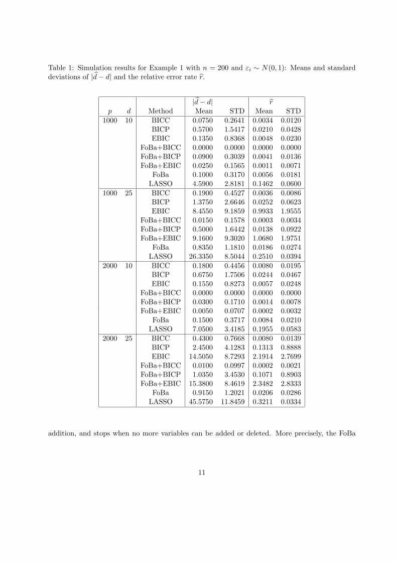
Table 1: Simulation results for Example 1 with n = 200 and εi ∼ N(0, 1): Means and standarddeviations of |d− d| and the relative error rate r.

|d− d| rp d Method Mean STD Mean STD

1000 10 BICC 0.0750 0.2641 0.0034 0.0120BICP 0.5700 1.5417 0.0210 0.0428EBIC 0.1350 0.8368 0.0048 0.0230

FoBa+BICC 0.0000 0.0000 0.0000 0.0000FoBa+BICP 0.0900 0.3039 0.0041 0.0136FoBa+EBIC 0.0250 0.1565 0.0011 0.0071

FoBa 0.1000 0.3170 0.0056 0.0181LASSO 4.5900 2.8181 0.1462 0.0600

1000 25 BICC 0.1900 0.4527 0.0036 0.0086BICP 1.3750 2.6646 0.0252 0.0623EBIC 8.4550 9.1859 0.9933 1.9555


FoBa 0.8350 1.1810 0.0186 0.0274LASSO 26.3350 8.5044 0.2510 0.0394

2000 10 BICC 0.1800 0.4456 0.0080 0.0195BICP 0.6750 1.7506 0.0244 0.0467EBIC 0.1550 0.8273 0.0057 0.0248


FoBa 0.1500 0.3717 0.0084 0.0210LASSO 7.0500 3.4185 0.1955 0.0583

2000 25 BICC 0.4300 0.7668 0.0080 0.0139BICP 2.4500 4.1283 0.1313 0.8888EBIC 14.5050 8.7293 2.1914 2.7699


FoBa 0.9150 1.2021 0.0206 0.0286LASSO 45.5750 11.8459 0.3211 0.0334

addition, and stops when no more variables can be added or deleted. More precisely, the FoBa

11

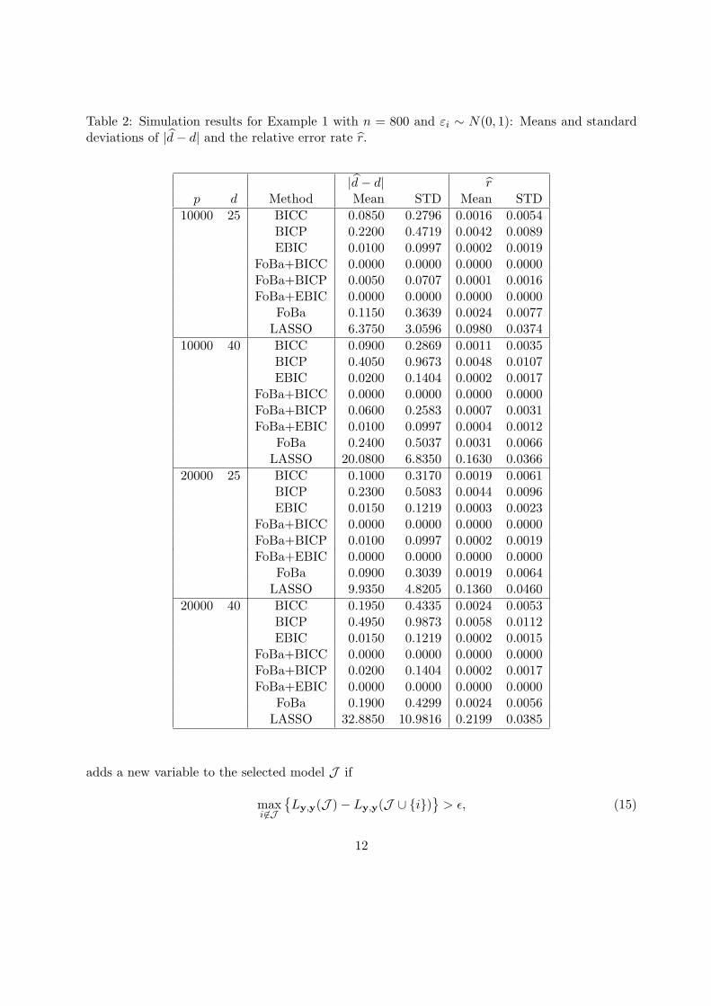
Table 2: Simulation results for Example 1 with n = 800 and εi ∼ N(0, 1): Means and standarddeviations of |d− d| and the relative error rate r.

|d− d| rp d Method Mean STD Mean STD

10000 25 BICC 0.0850 0.2796 0.0016 0.0054BICP 0.2200 0.4719 0.0042 0.0089EBIC 0.0100 0.0997 0.0002 0.0019


FoBa 0.1150 0.3639 0.0024 0.0077LASSO 6.3750 3.0596 0.0980 0.0374

10000 40 BICC 0.0900 0.2869 0.0011 0.0035BICP 0.4050 0.9673 0.0048 0.0107EBIC 0.0200 0.1404 0.0002 0.0017


FoBa 0.2400 0.5037 0.0031 0.0066LASSO 20.0800 6.8350 0.1630 0.0366

20000 25 BICC 0.1000 0.3170 0.0019 0.0061BICP 0.2300 0.5083 0.0044 0.0096EBIC 0.0150 0.1219 0.0003 0.0023


FoBa 0.0900 0.3039 0.0019 0.0064LASSO 9.9350 4.8205 0.1360 0.0460

20000 40 BICC 0.1950 0.4335 0.0024 0.0053BICP 0.4950 0.9873 0.0058 0.0112EBIC 0.0150 0.1219 0.0002 0.0015


FoBa 0.1900 0.4299 0.0024 0.0056LASSO 32.8850 10.9816 0.2199 0.0385

adds a new variable to the selected model J if

maxi 6∈J

Ly,y(J )− Ly,y(J ∪ i)

> ǫ, (15)

12

Table 3: Simulation results for Example 1 with εi ∼ N(0, σ2): Means and standard deviations of|d− d| and the relative error rate, where n = 800, p = 10000 and d = 25.

|d− d| rσ2 Method Mean STD Mean STD

4 BICC 0.2800 0.5596 0.0063 0.0133BICP 0.2900 0.5266 0.0067 0.0123EBIC 0.4150 0.6893 0.0088 0.0150

FoBa+BICC 0.1500 0.4103 0.0032 0.0087FoBa+BICC.1 0.6750 0.8620 0.0146 0.0192FoBa+BICC.2 2.1850 1.4286 0.0501 0.0358FoBa+BICP 0.1050 0.3530 0.0022 0.0075FoBa+EBIC 0.4150 0.6966 0.0089 0.0152

FoBa 0.3550 0.6566 0.0076 0.0143LASSO 5.2300 2.6328 0.0909 0.0348

9 BICC 1.4850 1.4283 0.0569 0.0370BICP 1.7850 1.3520 0.0485 0.0358EBIC 3.5600 1.9430 0.0884 0.0553


FoBa 0.8950 0.8471 0.0272 0.0236LASSO 3.3850 2.2963 0.1262 0.0448

16 BICC 4.7800 3.6508 0.1648 0.0616BICP 4.8000 2.2551 0.1383 0.0753EBIC 7.7000 2.6581 0.2421 0.1272


FoBa 8.3100 3.2133 0.1564 0.0403LASSO 2.4900 1.9231 0.1887 0.0588

25 BICC 10.7500 6.0623 0.2811 0.0687BICP 8.0650 2.6939 0.2691 0.1269EBIC 11.3100 2.8574 0.4569 0.2153


FoBa 29.0550 6.1220 0.2998 0.0310LASSO 4.3400 2.7718 0.2734 0.0851

13

where ǫ > 0 is a prescribed constant. After adding j = argmaxi 6∈J Ly,y(J )− Ly,y(J ∪ i) to

model J , the FoBa deletes a variable if

mini∈J ⋆

Ly,y(J ⋆\i)− Ly,y(J ⋆)

Ly,y(J )− Ly,y(J ⋆)< ν, (16)

where J ⋆ = J ∪ j, and ν ∈ (0, 1) is a prescribed constant. In our implementation below, we

set ǫ = 9.766 log(2p)/n and ν = 0.5.

While the idea of deleting all the redundant variables after each addition is appealing and may

improve the search, it is computationally more time-consuming than the algorithm presented in

section 2.2 with one-way forward search followed by one-way backward deletion, although the

difference is less substantial when p is large or very large, as then the computation of the initial

matrix L0 (see Remark 1(ii)) contributes a major part of the computing time for those greedy

algorithms.

Example 1. First we consider model (1) with all xij and εi independent N(0, 1). We let sample

size n = 200 or 800. For n = 200, we set the number of regression variables p = 1000 or 2000,

and the number of non-zero coefficients d = 10 or 25. For n = 800, we set p = 10000 or 20000,

and d = 25 or 40. The non-zero regression coefficients are of the form (−1)u(b + |v|), where

b = 2.5√

2 log p/n, u is a Bernoulli random variable with P (u = 1) = P (u = 0) = 0.5, and

v ∼ N(0, 1). For each setting, we replicate the simulation 200 times.

The simulation results are reported in Figure 1 which plots the selected numbers of regression

variables from the 200 replications in the ascending order. For BICP, BICC and EBIC, both d,

the number of variables selected by the forward search, and d, the number of variables selected by

the backward search, are plotted together. By the definitions, it holds that d ≥ d, though d = d

in most the replications. Note both LASSO and FoBa only produce one estimated model.

Figure 1 indicates that the algorithm with the BICP works well in the sense that d = d in most

replications, especially when n = 800. Both BICC and FoBa provide better performance in every

settings. When n = 200 and d = 25, EBIC tends to select too fewer covariates due to the heavier

penalty (than BICP) when the sample size n = 200. But for large samples with n = 800, BICC,

EBIC and FoBa perform about equally well. However the version of LASSO employed turned out

not competitive with the other four methods, although it has the advantage for knowing σ which

is not required by the other methods.

14

To have a fair comparisons on the different stopping rules used in the greedy searches, Figure

1 also includes the results from the using the FoBa algorithm but with both the stopping rules

(15) and (16) replaced by BICP, BICC or EBIC. Now the FoBa coupled with BICC seems to

further improve the performance. It is also clear that EBIC does not work as well as the other

stopping rules for small sample size n = 200.

Tables 1 and 2 present the means and the standard deviations of the absolute difference |d−d|in the 200 replications for the different estimation methods with n = 200 and 800 respectively.

Also listed are the means and the standard deviations of a relative error of a fitted model defined

as

r = (number of selected wrong variables

+ number of unselected true variables)/(2 d).

Similar to the pattern in Figure 1, BICP, BICC and FoBa provided comparable performances

while BICC is slightly better than FoBa, and BICP is slightly worse than FoBa. EBIC did not

performed well when n = 200. The improvement from using BICC as the stopping rule instead of

(15) and (16) in FoBa is also noticeable. However it is more striking that the LASSO estimation

so defined is not competitive in comparison with all the other greedy search methods, in spite of

its computational efficiency. Note that using λ = σ√

(log n)/n in (14) leads to poorer estimates.

To examine the robustness with respect to the signal-to-noise ratio, we repeated the simulation

with σ2 = Var(εi) = 4, 9, 16 and 25. To save the space, we only report the results from the setting

(n, p, d) = (800, 10000, 25); see Figure 2 and Table 3. As we would expect, the methods penalizing

log(RSS) such as BICP and EBIC are robust against the increase of σ2. The methods penalizing

RSS directly such as FoBa are less so. The version of LASSO method appeared to work well.

This is an artifact as we used λ = σ√2(log p)/n in (14) in the simulation with σ2 being the true

value of Var(εi). It is noticeable that BICC is less robust that BICP, as the choice of c0 should

depend on σ2; see (8).

Example 2. We use the same setting as in Example 1 with the added dependence structure as

follows: for any 1 ≤ k ≤ n and 1 ≤ i 6= j ≤ d,

Corr(Xki, Xkj) = (−1)u1(0.5)|i−j|, Corr(Xki, Xk,i+d) = (−1)u2ρ,

15

Corr(Xki, Xk,i+2d) = (−1)u3(1− ρ2)1/2,

where ρ is drawn from the uniform distribution on the interval [0.2, 0.8], and u1, u2 and u3

are independent and are of the same distribution as u in Example 1. All xki, for i > 3d, are

independent. We assume that the first d regression variables have the non-zero coefficients. The

simulation results are depicted in Figure 3 which shows the similar pattern to that of Figure 1,

although the performance is hampered slightly by the dependence among the regressors.

4 Main theoretical result

Theorem 2 below shows that with probability converging to 1, the estimator In,1 from the forward

addition alone contains the true model In, and with a backward deletion following the forward

addition, In,2 is a consistent estimator for In.We introduce some notation first. Let φmin(J ) and φmax(J ) denote, respectively, the minimum

and the maximum eigenvalues of X′JXJ /n. Let ψk be as in (11) and define

φk = min|J |=k

φmin(J ), φ∗k = max|J |=k

φmax(J ), (17)

mk = infm : dnφ

∗m/m < (1− γ)2φk−1ψk

. (18)

We will prove in the Appendix that the cardinality of the collection Ck in (12) is bounded by

|Ck| ≤∏k

j=1(mk − 1). Let ||xj ||2 = n for all 1 ≤ j ≤ p and In,µ, dn, β∗, c∗, γ, k∗1, k∗2 be as in (9)

and (10) with a fixed c∗ > 0. Some regularity conditions are now in order.

C1 (Conditions on dn, p, β∗ and k∗ = k∗1 ∧ k∗2)

β∗ ≥M0σ√2(log p)/n,

∑k∗

k=1 logmk ≤ η1 log p, (19)

with M0 ≥ (√1 + η1 +

√η1)/(c∗γ) and η1 > 0, and

dn ≤M1n/(2 log p), k∗(log p)/n = O(1), (k∗ + log p)/n→ 0, (20)

with c∗M20M1 < (c∗M0 −

√η1)

2/(1 + η0)− 1.

16

C2 (Adjustment for BICP) The estimators I1,n and I2,n are defined as in section 2.2 but with

BICPk adjusted by a factor (1 + η0) to

BICPk = logLy,y(Jk)/n+ 2k(1 + η0)(log p)/n, (21)

and BICP∗k adjusted in the same manner.

C3 (Additional condition on k∗ for backward deletion.)

log(k∗!) ≤ η2 log p with η1 + η2 ≤ min1 + η0, c∗(M0/2)2. (22)

Theorem 2 Suppose conditions C1 and C2 hold with η0 ≥ η1. Then,

PIn,1 ⊃ In, k < k∗, |σn,1 − σ| ≤ ǫ

→ 1 ∀ ǫ > 0, (23)

where σ2n,1 = ‖P⊥In,1

y‖2/(n− |In,1|). If in addition condition C3 hold, then

PIn,2 = In

→ 1 (24)

and the efficient estimation of µ, β and σ2 is attained with

µ = PIn,2

y, β = (X′In,2

XIn,2

)−1X′In,2

y, σ2n =‖(In −P

In,2)y‖2

n− |In,2|. (25)

Remark 2. (i) The sparse Riesz condition (Zhang and Huang, 2008) asserts

c∗ ≤ φd∗n ≤ φ∗d∗n ≤ c∗ (26)

with fixed 0 < c∗ < c∗ < ∞ and d∗n → ∞, which weakens the restricted isometry condition

(Candes and Tao 2005) by allowing c∗ − 1 6= 1− c∗. Such conditions are often used in the ‘large

p and and small n’ literature. Random matrix theory provides (26) with d∗n log(p/d∗n) = a0n for

fixed c∗, c∗ and certain small a0, allowing p≫ n. Under (26), k∗ = k∗1 ≤ d∗n in (9) for the vector

β when

dn log( e‖µ‖2c∗dnnβ2∗

)+ 1 + log

√dn/(2π) ≤ c∗(d

∗n − dn)

and for k∗ + dn ≤ d∗n,

mk ≤ dnc∗/(1− γ)2c2∗+ 1.

17

Thus, (26) can be viewed as a crude sufficient condition to guarantee manageable growth of

k∗ and |Ck| in conditions C1 and C3, with maxk≤k∗ mk = O(dn) and k∗ = O(dn) in the case

of ‖µ‖2 = O(dnnβ2∗). Under such scenarios, the main sparsity requirement of Theorem 2 is

dn log dn = O(log p).

(ii) Condition C1 requires that the non-zero regression coefficient in model (1) be at least of the

order O((log p)/n1/2

), the smallest order possible for consistent variable selection (Wainwright,

2009b; Zhang, 2007).

(iii) To prove the consistency in (23) and (24), we need to increase the penalty level in the

BICP by a fraction η0 as in condition C2. Meanwhile, conservative Bonferroni estimates of

multiple testing errors are used in all stages of the proofs of our theorems. For highly sparse β,

we prove in Theorem 3 that the conclusions of Theorem 2 holds for the simple BICP (5). Thus, it

is reasonable to use the slightly more aggressive (5) for both the forward and backward stopping

rules. Our simulation results, not reported here, also conforms with this recommendation.

Theorem 2 is proved in the appendix by showing that with high probability, (a) the forward

search stays within Jk ∈ Ck before it finds all variables with βj 6= 0, (b) BICP stops the forward

search as soon as all the variables with βj 6= 0 are found, and (c) the backward deletion deletes

exactly all falsely discovered variables in the forward addition. The fact (b) is of independent

interest, although it is not a consequence of Theorem 2.

For highly sparse β satisfying dn log dn ≤ (log log p)/2, a modification of Theorem‘2 provides

the selection consistency of the simpler and more explicit BICP in (5). We state this result in the

theorem below. Note that when dn is bounded, the conditions C1, C3 and (27) below are easily

fulfilled.

Theorem 3 Suppose condition C1 holds with η0 = 0 and

k∗∑

k=1

|Ck| ≪√log p. (27)

Then, (23) holds for the BICPk in (5). If in addition condition C3 holds, then (24) and (25) hold

for the BICPk in (5).

Although we focus in this paper on the BICP criterion, the methods developed for the proofs

18

can be used for investigating a number of related forward search procedures and also, for example,

the ℓ2- boosting of Buhlmann (2006).

5 Appendix

Here we prove Theorems 1, 2 and 3. We introduce technical lemmas and their proofs as needed.

The proof of Theorem 1 uses the following lemma to derive lower bounds for the reduction of

residual sum of squares in an approximate forward search.

Lemma 1 Let ψk be as in (11), β∗ in (9), µj,k = ‖PJk−1∪jP⊥Jk−1

µ‖ with a certain Jk−1 of size

|Jk−1| = k − 1, and µ∗k = maxj µj,k. Then,

|In \ Jk−1|(µ∗k)2 ≥ ψk−1‖P⊥Jk−1

µ‖2 ≥ ψ2k−1n

∑j∈In\Jk−1

β2j . (28)

In particular, for In \ Jk−1 6= ∅, µ∗k ≥ ψk−1√nβ∗.

Proof of Lemma 1. Let A = In ∪ Jk−1 and B = In \ Jk−1. By (11), φmin(A) ≥ ψk−1. Since

µj,k = 0 for j ∈ Jk−1 and ‖PJk−1xj‖2 ≤ n,

|B|(µ∗k)2 ≥∑

j∈B

|x′jP

⊥Jk−1

µ|2

n= µ′P⊥

Jk−1(XAX

′A/n)P

⊥Jk−1

µ.

This gives (28) since P⊥Jk−1

µ is in the column space of XA and ‖P⊥Jk−1

µ‖2 ≥ ψk−1n‖βB‖2 as in

Lemma 1 of Zhang and Huang (2008).

Proof of Theorem 1. Let km = mink : |Jk∩In| = m, Bm = In\Jkm and ξm = ‖βBm‖2/|Bm|.

Since kdn ≤ k∗2 iff ‖P⊥Jd∗

µ‖ = 0, we assume ‖P⊥Jd∗

µ‖ > 0. Since ‖PJkP⊥

Jk−1µ‖ ≥ (1 − γ)µ∗k,

Lemma 1 implies

kj∧k∗2∑

k=kj−1+1

ψ2k−1 ≤

kj∧k∗2∑

k=kj−1+1

‖PJkP⊥

Jk−1µ‖2

(1− γ)2nξj−1≤

‖PJkj∧k∗2

P⊥Jkj−1

µ‖2

(1− γ)2nξj−1. (29)

Since ξj−1 ≥ β2∗ and ‖PJkjP⊥

Jkj−1

µ‖2 ≤ ‖XBj−1βBj−1

‖2 ≤ nφmax(In)‖βBj−1‖2,

kdn∧k∗2∑

k=1

ψ2k−1 < min

‖µ‖2(1− γ)2nβ2∗

,φmax(In)dn(dn + 1)

2(1− γ)2

≤

k∗2∑

k=1

ψ2k−1.

19

The inequality is strict due to ‖P⊥Jd∗

µ‖ > 0. This gives kdn ≤ k∗2. For k∗1,

(1− γ)2kdn∧k

∗1∑

k=1

ψk−1 ≤dn∑

j=1

kj∧k∗1∑

k=kj−1∧k∗1+1

(m− j + 1)‖PJkP⊥

Jk−1µ‖2

max‖P⊥Jk−1

µ‖2, nc∗β2∗

≤dn∑

j=1

∫ ‖P⊥Jkj−1∧k∗

1

µ‖2

‖P⊥Jkj∧k∗

1

µ‖2

(m− j + 1)dx

maxx, nc∗β2∗

=

dn∑

j=1

∫ ‖PJk∗1

µ‖2

‖P⊥Jkj∧k∗

1

µ‖2

dx

maxx, nc∗β2∗.

Since ‖P⊥Jkj∧k∗

1

µ‖2 ≥ (dn − j)nc∗β2∗ and dn! > d

dn+1/2n e−dn

√2π by Stirling,

(1− γ)2kdn∧k

∗1∑

k=1

ψk−1 <

dn∑

j=1

∫ ‖µ‖2

(dn−j)c∗nβ2∗

dx

maxx, nc∗β2∗

= dn log( ‖µ‖2c∗nβ2∗

)+ 1− log((dn − 1)!)

< dn log( e‖µ‖2c∗dnnβ2∗

)+ 1 + log

√dn/(2π).

This gives kdn ≤ k∗1 by (9).

The proof of Theorem 2 requires two lemmas. Lemma 2 provides upper bounds for the

cardinality of the collection of models in (12), while Lemma 3 gives a sharp large deviation bound

for the tail of the t-distribution.

Lemma 2 For the Ck,mk in (12) and (18), |Ck| ≤∏k

m=1(mk − 1).

Proof of Lemma 2. It suffices to prove #j : µj,k ≥ (1− γ)µ∗k ≤ mk − 1 for all k. For a fixed

Jk−1, let v = P⊥Jk−1

µ, x⊥j = P⊥

Jk−1xj and sj = sgn(x′

jv). For any A ⊂j : µj,k ≥ (1 − γ)µ∗k

,

(28) gives

∑

j∈A

µj,k‖v‖ ≥ |A|(1− γ)µ∗k/‖v‖ ≥ |A|(1− γ)

√ψk−1/|In \ Jk−1|.

On the other hand, for |A| ≤ mk, the upper bound in (17) gives

∑

j∈A

sjx′jv

‖v‖ ≤∥∥∥∑

j∈A

sjxj

∥∥∥ ≤(nφ∗mk

∑

j∈A

s2j

)2=

√nφ∗mk

|A|.

20

Since µj,k = |x′jv|/‖x⊥

j ‖ ≤ |x′jv|/

√φkn, the above two inequalities yield

|A| ≤ mk ⇒ |A| ≤ φ∗mk|In \ Jk−1|

(1− γ)2φkψk−1< mk

in view of the definition of mk in (18). This gives #j : µj,k ≥ (1− γ)µ∗k < mk.

Lemma 3 Let Tm have the t-distribution with m degrees of freedom, or equivalently T 2m ∼ F1,m.

Then, there exists ǫm → 0 such that for all t > 0

PT 2m > m(e2t

2/(m−1) − 1)≤ 1 + ǫm√

πte−t2 . (30)

Proof of Lemma 3. Let x =√m(e2t2/(m−1) − 1). Since Tm has the t-distribution,

PT 2m > x2

=

2Γ((m+ 1)/2)

Γ(m/2)√mπ

∫ ∞

x

(1 +

u2

m

)−(m+1)/2du

≤ 2Γ((m+ 1)/2)

xΓ(m/2)√mπ

∫ ∞

x

(1 +

u2

m

)−(m+1)/2udu

=2Γ((m+ 1)/2)m

xΓ(m/2)√mπ(m− 1)

(1 +

x2

m

)−(m−1)/2.

Since x ≥ t√2m/(m− 1),

PT 2m > x2

≤

√2Γ((m+ 1)/2)

Γ(m/2)√m− 1

e−t2

t√π= (1 + ǫm)

e−t2

t√π,

where ǫm =√2Γ((m+ 1)/2)/Γ(m/2)

√m− 1 − 1 → 0 as m→ ∞.

Proof of Theorem 2. We prove P∩5j=1Ωj → 1 in five steps, where

Ω1 =Jk ∈ Ck ∀ ‖P⊥

Jk−1µ‖ > 0

, Ω2 =

‖P⊥

Jkµ‖ = 0, k ≥ k

,

Ω3 =‖P⊥

Jkµ‖ > 0, k < k

, Ω4 =

|σn,1 − σ| ≤ ǫ

, Ω5 =

In = In,2

.

In ∩5j=1Ωj , the forward search finds all variables with βj 6= 0 reasonably quickly by Theorem 1, the

stopping rule k does not stop the forward search too early, k stops the forward search immediately

after finding all βj 6= 0, the estimation error for σ is no greater than ǫ, and the backward deletion

removes all extra variables. Let Φ(t) be the standard normal distribution function.

Step 1. We prove PΩc1 → 0. This does not involve the stopping rule for the forward search.

Let zj,k = ‖PJk−1∪jP⊥Jk−1

ε‖ and j∗k = argmaxj µj,k. Since ‖PJ∪jP⊥Jv‖2 = L2

v,xj(J )/Lxj ,xj

(J ),

21

(6) implies µ∗k − µjk,k ≤ zj∗k,k + maxj zj,k. Since ‖PJ∪jP

⊥J ε‖/σ ∼ |N(0, 1)| for deterministic

J , j and µ∗k ≥ ψk−1√nβ∗ ≥ c∗

√nβ∗ ≥ c∗M0σ

√2 log p by Lemma 1 and (19),

PJk 6∈ Ck, µ

∗k > 0,Jk−1 ∈ Ck−1

≤ Pzj∗

k,k +max

jzj,k ≥ γc∗M0σ

√2 log p, Jk−1 ∈ Ck−1

≤ 2p|Ck−1|Φ(−√(1 + η1)2 log p

)+ 2|Ck−1|Φ

(−√η12 log p

),

due to γc∗M0 ≥√1 + η1+

√η1. Thus, since |Ck−1| ≤

∏k−1ℓ=1 (mℓ−1) by Lemma 2 and

∑k∗

k=1 logmk ≤η1 log p by (19), (13) gives

PΩc1

≤

k∗∑

k=1

2|Ck−1|pΦ

(−√(1 + η1)2 log p

)+Φ

(−

√η12 log p

)

≤ eη1 log ppΦ

(−√(1 + η1)2 log p

)+Φ

(−√η12 log p

)→ 0.

Step 2. We prove PΩ1 ∩ Ωc2 → 0. Let an = e2(1+η0)(log p)/n − 1. By (21)

BICPk < BICPk−1 ⇔ ‖PJkP⊥

Jk−1y‖2/‖P⊥

Jk−1y‖2 > an/(1 + an). (31)

Let ǫ0 > 0 be small and Ak = Jk ∪ In. Consider events

Ω2,k =‖PJk

P⊥Jk−1

y‖ ≥ µ∗k − σ√2η1 log p > 0,

‖PAk−1ε‖ ≤ ǫ0σ

√n, |(σ2n)−1‖ε‖2 − 1| ≤ ǫ0

.

It follows from Lemma 1 that in the event Ω2,k,

‖P⊥Jk−1

y‖2 = ‖PAk−1P⊥

Jk−1y‖2 + ‖P⊥

Ak−1ε‖2

≤ ‖P⊥Jk−1

µ‖2 + 2‖P⊥Jk−1

µ‖ × ‖PAk−1ε‖+ ‖ε‖2

≤ (1 + ǫ0)dn(µ∗k)

2/ψk−1 + (1 + 2ǫ0)σ2n.

Since µ∗k ≥ c∗M0σ√2 log p as in Step 1 with c∗M0 >

√η1, we have in Ω2,k,

‖PJkP⊥

Jk−1y‖2

‖P⊥Jk−1

y‖2 ≥ (µ∗k − σ√2η1 log p)

2

(1 + ǫ0)dn(µ∗k)2/ψk−1 + (1 + 2ǫ0)σ2n

≥ (2 log p)(c∗M0 −√η1)

2

(1 + ǫ0)dn(c∗M0)2(2 log p)/c∗ + (1 + 2ǫ0)n.

22

Since log p = o(n) by (20), an/(1+ an) ≤ (1+ ǫ0)(1+ η0)(2 log p)/n for k ≤ k∗ and large n. Thus,

for sufficiently small ǫ0 > 0 and in Ω2,k,

‖PJkP⊥

Jk−1y‖2

‖P⊥Jk−1

y‖2an/(1 + an)≥ (c∗M0 −

√η1)

2/(1 + η0)(1 + ǫ0)(1 + ǫ0)c∗M2

0 (2dn log p)/n+ (1 + 2ǫ0)> 1,

due to c∗M20 (2dn log p)/n ≤ c∗M

20M1 < (c∗M0−

√η1)

2/(1+η0)−1 by (20). Thus, Ω2 ⊇ ∩k∗

k=1Ω2,k

and as in the probability calculation in Step 1,

PΩ1 ∩ Ωc2 − P

|(σ2n)−1‖ε‖2 − 1| ≤ ǫ0

≤k∗∑

k=1

P‖PJk−1∪j

∗kP

⊥Jk−1

ε‖ > σ√

2η1 log p, Jk−1 ∈ Ck−1

+k∗∑

k=1

P‖PAk−1

ε‖ > ǫ0σ√n,Jk−1 ∈ Ck−1

≤k∗∑

k=1

|Ck−1|(Φ(−√

2η1 log p)+ P

χ2dn+k−1 > ǫ20n

)

≤ pη1Φ(−√2η1 log p

)+ o(1) = o(1),

since P√χ2d >

√d+ t ≤ Φ(−t) and ǫ0

√n−

√dn + k∗ ≫ √

2η1 log p.

Step 3. We prove PΩ1 ∩ Ω2 ∩ Ωc3 → 0. It follows from (31) that

BICPk < BICPk−1 ⇔ ‖PJkP⊥

Jk−1y‖2/‖P⊥

Jky‖2 > an, (32)

which is an F1,n−k test for the random model Jk against Jk−1. Since k(log p)/n ≤ k∗(log p)/n =

O(1), by Lemma 3 the threshold (n−k)an gives an F1,n−k-test of size O(1)p−1−η0+(k+1)/n/√log p .

p−1−η0/√log p. Since η0 ≥ η1 in (19),

PΩ1 ∩ Ω2 ∩ Ωc3 ≤

k∗∑

k=1

Pµ∗k = 0,BICPk < BICPk−1,Jk−1 ∈ Ck−1

.

k∗∑

k=1

(p− k + 1)|Ck−1|p1+η0

√log p

=pη1

pη0√log p

= o(1). (33)

Step 4. We prove PΩ1 ∩ Ωc4 → 0. Consider a fixed ǫ > 0. In Ω1 ∩ Ω2,k, k = k implies

‖PIn,1ε‖ = ‖PAk−1

ε‖ ≤ ǫ0σ√n and |(σ2n)−1‖ε‖2 − 1| ≤ ǫ0. Since |In,1| ≤ k∗ = o(n) and

‖P⊥In,1

y‖2 = ‖ε‖2−‖PIn,1ε‖2, for sufficiently small ǫ0, (σ−ǫ)2 ≤ ‖PIn,1

⊥ y‖2/(n− k) ≤ (σ+ǫ)2.

Thus, PΩ1 ∩ Ωc4 ≤ ∑

k≤k∗ PΩ1 ∩ Ωc2,k → 0 by Step 2.

23

Step 5. We prove PΩ1 ∩ Ω2 ∩ Ω3 ∩ Ωc5 → 0. Let

Ω5,k =maxj∈J ∗

k

‖PJ ∗kP⊥

J ∗k\jε‖2/σ2 < (η1 + η2)2 log p,

maxj 6∈In

‖PJ ∗kP⊥

J ∗k\jε‖2/‖P⊥

J ∗kε‖2 ≤ an,J ∗

k ⊃ In. (34)

In the event J ∗k ⊃ In, minj∈In ‖PJ ∗

kP⊥

J ∗k\jµ‖ ≥ β∗

√c∗ ≥M0σ

√c∗2(log p)/n. Since (c∗M0/2)

2 ≥η1 + η2 and P⊥

Jy = P⊥J ε for J ⊇ In, in the event Ω5,k,

minj∈In

‖PJ ∗kP⊥

J ∗k\jy‖ − max

j∈J ∗k\In

‖PJ ∗kP⊥

J ∗k\jy‖

> β∗√c∗ − 2σ

√(η1 + η2)2 log p ≥ 0,

so that the backward deletion does not delete the elements of In for k > dn. Moreover, since

the forward addition and backward deletion are based on the same tests, by (32) and the second

inequality in Ω5,k, the backward deletion does not stop in for k > dn. Thus,

PΩ1 ∩ Ω2 ∩ Ω3 ∩ Ωc

5

≤ PJ ∗dn = In, k < dn

+

k∗∑

k=dn+1

PΩ1 ∩ Ω2 ∩ Ω3 ∩ Ωc

5,k

.

In Ω1∩Ω2∩Ω3, k = k implies In ⊂ In,1 = Jk and Jk ∈ Ck, so that the backward deletion involves

at most N∗k−1 combinations of j,J ∗

k , where N∗k = (k∗!/k!)

∑k∗

k=1 |Ck| ≤ pη2+η1/k!. Since the

inequalities in (34) involve χ21 and F1,n−k variables in random models,

k∗∑

k=dn+1

PΩ1 ∩ Ω2 ∩ Ω3 ∩ Ωc

5,k

. (35)

≤∑

k

pη1+η2

(k − 1)!

(Pχ2

1 > 2(η1 + η2) log p+ PF1,n−k > (n− k)an)→ 0.

Since η1 + η2 ≤ 1 + η0, the bound here for the tail of F1,n−k is identical to that of Step 3. The

proof of PJ ∗dn

= In, k < dn→ 0 is simpler than Step 2 and omitted. This completes the step.

Proof of Theorem 3. For the BICPk in (5), an = e2(log p)/n − 1. Since k∗(log p)/n = O(1),

the size of the test F1,n−k > (n − k)an is O(p−1(log p)−1/2) by Lemma 3 uniformly for k ≤ k∗.

Since the condition η0 ≥ η1 is used only in (33), the proof of Theorem 2 is still valid when∑k∗

k=1 |Ck| ≪√log p.

24

References

[1] An, H. and Gu, L. (1985). On the selection of regression variables. ACTA MathematicaeApplicatae Sinica, 2, 27-36.

[2] An, H. and Gu, L. (1987). Fast stepwise procedures of selection of variables by using AICand BIC criteria. ACTA Mathematicae Applicatae Sinica, 5, 60-67.

[3] Bickel, P., Ritov Y. and Tsybakov, A. (2009). Simultaneous analysis of Lasso andDantzig selector. Ann. Statist. 37 1705-1732.

[4] Buhlmann, P. (2006). Boosting for high-dimensional linear models. Ann. Statist. 34 559-583.

[5] Bunea, F. (2008). Honest variable selection in linear and logistic regression models via ℓ1and ℓ1 + ℓ2 penalization. Electronic Journal of Statistics, 2 11531194.

[6] Bunea, F., Tsybakov, A. and Wegkamp, M. (2007). Sparsity oracle inequalities for thelasso. Electron. J. Statist. 1 169-194 (electronic).

[7] Candes, E. and Tao, T. (2005). Decoding by linear programming. IEEE Trans. Inform.Theory 51 4203-4215.

[8] Candes, E. and Tao, T. (2007). The Dantzig selector: statistical estimation when p is muchlarger than n (with discussion). Ann. Statist. 35 2313-2404.

[9] Chen, J. and Chen, Z. (2008). Extended Bayesian information criteria for model selectionwith large model spaces. Biometrika, 95, 759-771.

[10] Fan, J. and Li, R. (2001). Variable selection via nonconcave penalized likelihood and itsoracle properties. J. Amer. Statist. Assoc. 96 13481360.

[11] Fan, J. and Lv, J. (2008). Sure independence screening for ultra-high dimensional featurespace. J. Roy. Stats. Soc. B, 70, 849-911.

[12] Fan, J. and Peng, H. (2004). On non-concave penalized likelihood with diverging numberof parameters. Ann. Stats. 32 928-961.

[13] Greenshtein E. and Ritov Y. (2004). Persistence in high-dimensional linear predictorselection and the virtue of overparametrization. Bernoulli 10 971-988.

[14] Huang, J., Ma, S. and Zhang, C.-H. (2008). Adaptive LASSO for sparse high-dimensionalregression models. Statistica Sinica 18 1603-1618.

[15] Knight, K. and Fu, W. J. (2000). Asymptotics for lasso-type estimators. Ann. Statist. 281356-1378.

[16] Mallows, C.L. (1973). Some comments on Cp. Technometrics 12 661-675.

[17] Mallat, S. and Zhang, Z. (1993). Matching pursuits with time-frequency dictionaries.IEEE Transa. Signal Processing 41 3397-3415.

25

[18] Meinshausen, N. andBuhlmann, P. (2006) High dimensional graphs and variable selectionwith the Lasso. Ann. Statist. 34 1436-1462.

[19] Meinshausen, N. and Yu, B. (2009). Lasso-type recovery of sparse representations forhigh-dimensional data. Ann. Statist. 37 246-270.

[20] Schwarz, G. (1978). Estimating the dimension of a model. Ann. Statist. 6 461-464.

[21] Tibshirani, R. (1996). Regression shrinkage and selection via the Lasso. J. Roy. Statist.Soc. Ser. B 58 267-288.

[22] Tropp, J.A. (2006). Just relax: convex programming methods for identifying sparse signalsin noise. IEEE Trans. Inform. Theory 52 1030-1051.

[23] van de Geer, S. (2008). High-dimensional generalized linear models and the Lasso. Ann.Statist. 36 614-645.

[24] Wainwright, M.J. (2009a). Sharp thresholds for noisy and high-dimensional recovery ofsparsity using ℓ1-constrained quadratic programming (Lasso). IEEE Trans. Info. Theory 55

2183–2202.

[25] Wainwright, M.J. (2009b). Information-theoretic limitations on sparsity recovery in thehigh-dimensional and noisy setting. IEEE Trans. Info. Theory 55 5728–5741.

[26] Zhang, C.-H. (2007). Information-theoretic optimality of variable selection with concavepenalty. Technical Report 2007-008, Department of Statistics and Biostatistics, Rutgers Uni-versity.

[27] Zhang, C.-H. (2008). Discussion: One-step sparse estimates in nonconcave penalized likeli-hood models. Ann. Statist. 36 1553-1560.

[28] Zhang, C.-H. (2010). Nearly unbiased variable selection under minimax concave penalty.Ann. Statist. 38 894-942.

[29] Zhang, C.-H. and Huang, J. (2008). The sparsity and bias of the LASSO selection inhigh-dimensional regression. Ann. Statist. 36 1567-1594.

[30] Zhang, T. (2009a). Some sharp performance bounds for least squares regression with L1

regularization. Ann. Statist. 37 2109-2144.

[31] Zhang, T. (2009b). Adaptive forward-backward greedy algorithm for sparse learning withlinear models. In NIPS 2008, Koller, Schuurmans, Bengio and Bottou, Eds. pages 1921-1928.

[32] Zhao, P. andYu, B. (2006). On model selection consistency of LASSO. J. Machine LearningResearch 7 2541-2567.

[33] Zou, H. (2006). The adaptive lasso and its oracle properties. J. Amer. Statist. Assoc. 1011418-1429.

26

050

150

0 20 40 60 80

BIC

C

(n,p)=(200,1000)

050

150

0 20 40 60 80

BIC

P

050

150

0 20 40 60 80

EB

IC

050

150

0 20 40 60 80

Fo

Ba+B

ICC

050

150

0 20 40 60 80

Fo

Ba+B

ICP

050

150

0 20 40 60 80

Fo

Ba+E

BIC

050

150

0 20 40 60 80

Fo

Ba

050

150

0 20 40 60 80

LA

SS

O

050

150

0 20 40 60 80

(n,p)=(200,2000)

050

150

0 20 40 60 80

050

150

0 20 40 60 80

050

1500 20 40 60 80

050

150

0 20 40 60 80

050

150

0 20 40 60 80

050

150

0 20 40 60 80

050

150

0 20 40 60 80

050

150

0 20 40 60 80

(n,p)=(800,10000)

050

150

0 20 40 60 80

050

150

0 20 40 60 80

050

150

0 20 40 60 80

050

150

0 20 40 60 80

050

150

0 20 40 60 80

050

150

0 20 40 60 80

050

150

0 20 40 60 80

050

150

0 20 40 60 80

(n,p)=(800,20000)

050

150

0 20 40 60 80

050

150

0 20 40 60 80

050

150

0 20 40 60 80

050

150

0 20 40 60 80

050

150

0 20 40 60 80

050

150

0 20 40 60 80

050

150

0 20 40 60 80

Figure 1: Simulation results for Example 1 with εi ∼ N(0, 1). Plots of the numbers of selected

regression variables by the forward search and backward search in 200 replications. Two upper

rows with n = 200: d = 10 (solid lines), and d = 25 (dashed lines). Two lower rows with n = 800:

d = 25 (solid lines), and d = 40 (dashed lines).

27

0 50 150

020

4060

80

BICC

σ2=

4

0 50 150

020

4060

80

BICP

0 50 150

020

4060

80EBIC

0 50 150

020

4060

80

FoBa+BICC

0 50 150

020

4060

80

FoBa+BICP

0 50 150

020

4060

80

FoBa+EBIC

0 50 150

020

4060

80

FoBa

0 50 150

020

4060

80

LASSO

0 50 150

020

4060

80

BICC

σ2=

9

0 50 150

020

4060

80

BICP

0 50 150

020

4060

80

EBIC

0 50 150

020

4060

80

FoBa+BICC

0 50 150

020

4060

80

FoBa+BICP

0 50 150

020

4060

80

FoBa+EBIC

0 50 150

020

4060

80

FoBa

0 50 150

020

4060

80

LASSO

0 50 150

020

4060

80

BICC

σ2=

16

0 50 150

020

4060

80

BICP

0 50 150

020

4060

80

EBIC

0 50 150

020

4060

80

FoBa+BICC

0 50 150

020

4060

80

FoBa+BICP

0 50 150

020

4060

80

FoBa+EBIC

0 50 1500

2040

6080

FoBa

0 50 150

020

4060

80

LASSO

0 50 150

020

4060

80

BICC

σ2=

25

0 50 150

020

4060

80

BICP

0 50 150

020

4060

80

EBIC

0 50 150

020

4060

80

FoBa+BICC

0 50 150

020

4060

80

FoBa+BICP

0 50 150

020

4060

80

FoBa+EBIC

0 50 150

020

4060

80

FoBa

0 50 150

020

4060

80

LASSO

Figure 2: Simulation results for Example 1 with εt ∼ N(0, σ2): Plots of the numbers of selected

regression variables in 200 replications, where (n, p, d) = (800, 10000, 25).

28

050

150

0 20 40 60 80

BIC

C

(n,p)=(200,1000)

050

150

0 20 40 60 80

BIC

P

050

150

0 20 40 60 80

EB

IC

050

150

0 20 40 60 80

Fo

Ba+B

ICC

050

150

0 20 40 60 80

Fo

Ba+B

ICP

050

150

0 20 40 60 80

Fo

Ba+E

BIC

050

150

0 20 40 60 80

Fo

Ba

050

150

0 20 40 60 80

LA

SS

O

050

150

0 20 40 60 80

(n,p)=(200,2000)

050

150

0 20 40 60 80

050

150

0 20 40 60 80

050

1500 20 40 60 80

050

150

0 20 40 60 80

050

150

0 20 40 60 80

050

150

0 20 40 60 80

050

150

0 20 40 60 80

050

150

0 20 40 60 80

(n,p)=(800,10000)

050

150

0 20 40 60 80

050

150

0 20 40 60 80

050

150

0 20 40 60 80

050

150

0 20 40 60 80

050

150

0 20 40 60 80

050

150

0 20 40 60 80

050

150

0 20 40 60 80

050

150

0 20 40 60 80

(n,p)=(800,20000)

050

150

0 20 40 60 80

050

150

0 20 40 60 80

050

150

0 20 40 60 80

050

150

0 20 40 60 80

050

150

0 20 40 60 80

050

150

0 20 40 60 80

050

150

0 20 40 60 80

Figure 3: Simulation results for Example 2: Plots of the numbers of selected regression variables

by the forward search and backward search in 200 replications. Ten upper panels: n = 200,

d = 10 (solid lines), and d = 25 (dashed lines). Ten lower panels: n = 800, d = 25 (solid lines),

and d = 40 (dashed lines).

29

Documents

StepwiseSearchingfor FeatureVariables in High ...stats.lse.ac.uk/q.yao/qyao.links/paper/ahyz08.pdf · StepwiseSearchingfor FeatureVariables in High-DimensionalLinearRegression