Stereo Fusion: Combining Refractive

and Binocular Disparity

Seung-Hwan Baek Min H. Kim⇤

KAIST, 291 Daehak-ro, Yuseong-gu, Daejeon, South Korea

Abstract

The performance of depth reconstruction in binocular stereo relies on how ad-

equate the predefined baseline for a target scene is. Wide-baseline stereo is

capable of discriminating depth better than the narrow-baseline stereo, but it

often suffers from spatial artifacts. Narrow-baseline stereo can provide a more

elaborate depth map with fewer artifacts, while its depth resolution tends to be

biased or coarse due to the short disparity. In this paper, we propose a novel

optical design of heterogeneous stereo fusion on a binocular imaging system with

a refractive medium, where the binocular stereo part operates as wide-baseline

stereo, and the refractive stereo module works as narrow-baseline stereo. We

then introduce a stereo fusion workflow that combines the refractive and binoc-

ular stereo algorithms to estimate fine depth information through this fusion

design. In addition, we propose an efficient calibration method for refractive

stereo. The quantitative and qualitative results validate the performance of our

stereo fusion system in measuring depth in comparison with homogeneous stereo

approaches.

Keywords: stereo fusion, refractive stereo, multi-view stereo

1. Introduction

There have been many approaches to acquiring depth information of real scenes

such as passive stereo [1], active stereo [2], time-of-flight imaging [3], depth

⇤e-mail addresses: {shwbaek;minhkim(corresponding author)}@vclab.kaist.ac.kr

Preprint submitted to Computer Vision and Image Understanding February 14, 2016

(a) Binocular stereo(high depth resolution)

Scene

(b) Refractive stereo(high spatial resolution)

(c) Stereo fusion (high spatial and depth resolution)

Figure 1: (a) Binocular stereo detects depth accurately, whereas it suffers from spatial arti-

facts caused by occlusions and featureless regions. (b) Refractive stereo improves the spatial

resolution with fewer artifacts, but its depth resolution is coarse with fewer steps. (c) Our

stereo fusion significantly improves both spatial and depth resolution by combining these two

heterogeneous stereo methods.

from defocus [4], etc. Among them, passive stereo imaging has been commonly

used for distant measurements to understand scene shapes. Classical stereo algo-

rithms employ a pair of binocular stereo images. Such stereo algorithms estimate

depth by evaluating the distance of corresponding features, so-called disparity,

via computing matching costs and aggregating the costs [1]. However, owing to

the nature of triangulation in depth estimation, depth accuracy strongly depends

on the baseline between a stereo pair. For instance, a wide baseline elongates

the range of the correspondence search so that the matching problem cannot be

solved with high precision in typical locally-optimizing approaches [5]. On the

contrary, a narrow baseline shortens the resolution of disparity; therefore, the

accuracy of estimated depth could be degraded [6, 7].

Recently, Gao and Ahuja [8, 9] introduced a single-depth camera based on

refraction. Chen et al. [10] further extended this refractive mechanism. Such

refractive stereo systems estimate depth from the change of light direction;

therefore, the disparity in refractive stereo in general is smaller than that in

binocular stereo, i.e., its performance is similar to that of binocular stereo with

a narrow baseline.

We take inspiration from refractive stereo to combine these two heteroge-

2

neous stereo systems, where a stereo fusion system is designed with a refractive

medium placed on one of the binocular stereo cameras. In this paper, we in-

troduce a novel optical design that combines binocular and refractive stereo

and its depth process workflow that allows us to fuse heterogeneous stereo in-

puts seamlessly to achieve fine depth estimates. Our system comprises a pair

of stereo cameras, one of which is covered with a transparent medium, allowing

for enhanced depth accuracy. The proposed approach offers benefits compared

to the typical multiview stereo [7] in terms of building cost as our system em-

ploys just the same number of cameras as a binocular stereo does. It is also

more advantageous than multiview stereo, which consists of two cameras on a

linear slider [11], by providing physical stability, i.e., spinning the medium is

less undemanding than moving a camera on the slider frequently at different

distances.

The refractive calibration process that we propose in this paper is a natural

evolution of our previously published research [12]. We increase the efficiency of

the tedious refractive calibration process in the prior work [12]. In this paper, we

propose a novel refractive calibration method that requires fewer angle samples

(at least three angles), rather than the dense angle samples, from 0 to 360 degrees

at 10-degree intervals. As such, the novel calibration method can accelerate the

cumbersome calibration process that hinders the usefulness of refractive stereo.

We believe that this calibration method increases the usefulness of the proposed

stereo fusion method.

Figure 1 shows a brief overview of our method. The following contributions

have been made:

· A stereo fusion system that combines refractive and binocular

stereo. We propose a stereo fusion system that combines a refractive

medium on a binocular base. The medium is placed in front of a camera

in binocular stereo.

· Calibration methods for stereo fusion. We develop a workflow of cal-

ibration for this fusion system that includes radiometric, geometric and

3

refractive calibration methods. In particular, we propose an efficient cali-

bration method of refractive stereo based on xyz-Euler angles, which re-

quires a smaller number of angle measurements (at least three angles),

rather than dense measurements of complete angle variation. This cali-

bration enables us to obtain the essential points of the entire angles from

sub-sampled angle measurements.

· Depth fusion workflow that combines two heterogeneous stereo

images. Our calibration methods allow us to estimate depth from two

heterogeneous stereos. The resulting depth map achieves a higher depth

resolution with fewer artifacts than that of traditional homogeneous stereo.

2. Binocular vs. Refractive Disparity

This section describes the foundational differences of binocular and refractive

stereo, surveying state-of-the-art depth-from-stereo methods.

2.1. Multi-Baseline Stereo

Binocular disparity in stereo imaging describes pixel-wise displacement of par-

allax between corresponding points on a pair of stereo images taken from dif-

ferent positions. Searching correspondence on an epipolar line is necessary prior

to computing disparity. As disparity d depends on its depth, we can recover the

depth z using simple trigonometry as follows:

z = fb/d, (1)

where f is the focal length of the camera lens, and b is the distance between the

center of projections for the two cameras, the so-called baseline. In particular,

the baseline b determines the depth resolution of the stereo system, and b is also

related with occlusion error. Therefore, baseline must be adapted to the scene

configuration for optimal performance. There is no universal configuration of

baseline for real-world conditions.

4

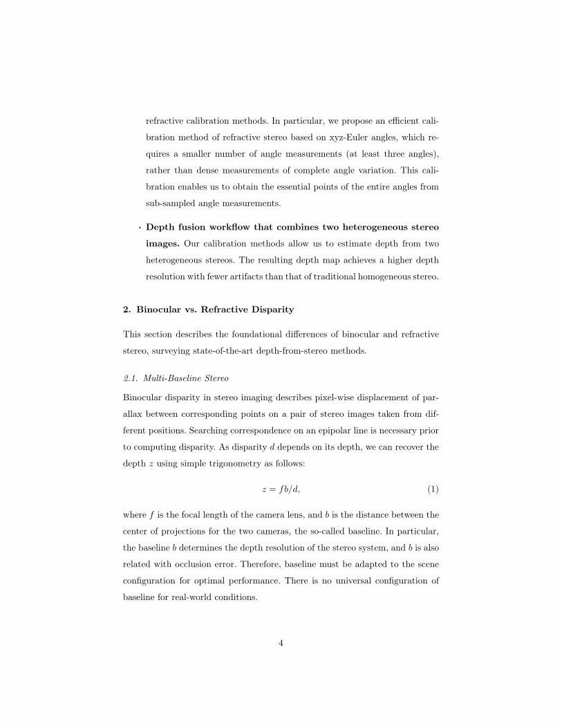
Wide-baseline stereo reserves more pixels for disparity than narrow-baseline

stereo does. Therefore, wide-baseline systems can discriminate depth with a

higher resolution. On the other hand, the search range of correspondences in-

creases, and in turn, it increases the chances of false matching. The estimated

disparity map is plausible in terms of depth, but it includes many small regions

without depth as spatial artifacts (of holes) on the depth map. This missing

information is caused by occlusion and false matching in featureless or pattern-

repeated regions, where the corresponding point search fails.

Narrow-baseline stereo has a relatively short search range of correspondence.

The search range of correspondence is shorter than that of wide-baseline stereo.

There are fewer chances for false matching, so accuracy and efficiency in cost

computation can be enhanced. In addition, the level of spatial noise in the dis-

parity map is low because the occluded area is small. However, narrow-baseline

stereo reserves a small number of pixels for depth discrimination. The depth-

discriminative power decreases accordingly, whereas the spatial artifacts in the

disparity map are reduced. It trades off the discriminative power for the reduced

spatial artifacts in the disparity map.

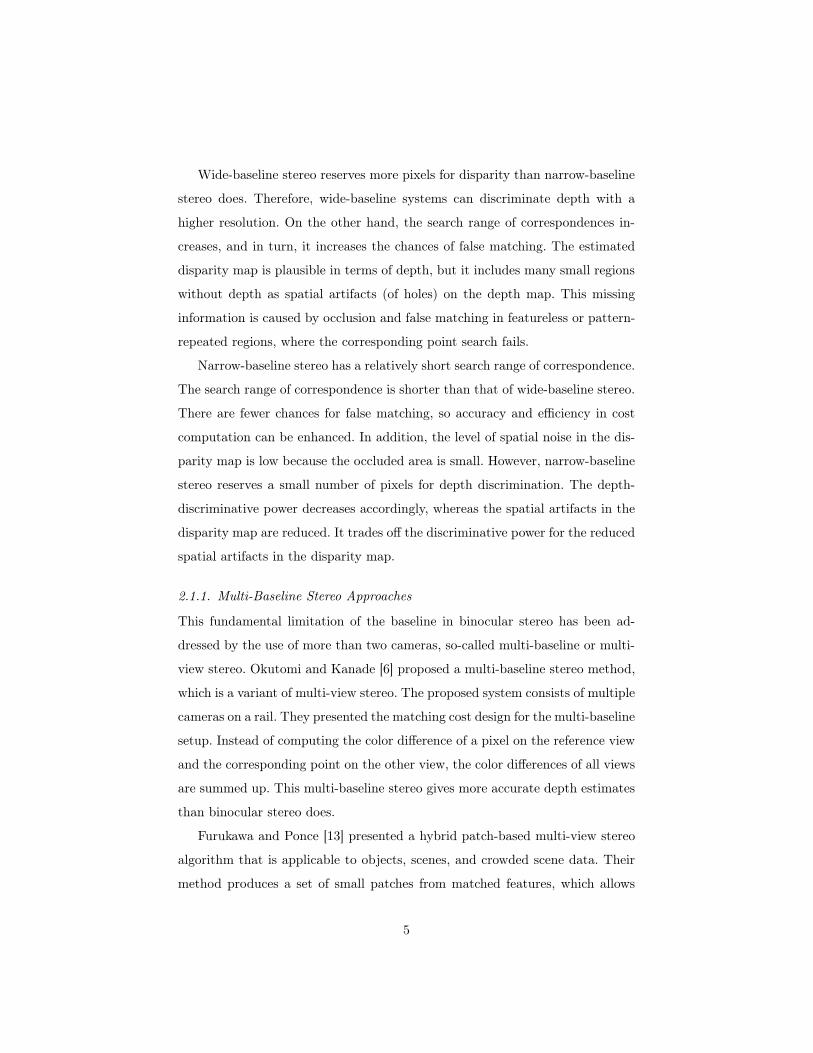
2.1.1. Multi-Baseline Stereo Approaches

This fundamental limitation of the baseline in binocular stereo has been ad-

dressed by the use of more than two cameras, so-called multi-baseline or multi-

view stereo. Okutomi and Kanade [6] proposed a multi-baseline stereo method,

which is a variant of multi-view stereo. The proposed system consists of multiple

cameras on a rail. They presented the matching cost design for the multi-baseline

setup. Instead of computing the color difference of a pixel on the reference view

and the corresponding point on the other view, the color differences of all views

are summed up. This multi-baseline stereo gives more accurate depth estimates

than binocular stereo does.

Furukawa and Ponce [13] presented a hybrid patch-based multi-view stereo

algorithm that is applicable to objects, scenes, and crowded scene data. Their

method produces a set of small patches from matched features, which allows

5

the gaps between neighboring feature points to be filled in, yielding a fine mesh

model. Gallup et al. [14] estimated the depth of a scene by adjusting the base-

line and the resolutions of images from multiple cameras so that depth estima-

tion becomes computationally efficient. This system exploits the advantages of

multi-baseline stereo while requiring the mechanical support of moving cameras.

Nakabo et al. [11] presented a variable-baseline stereo system on a linear slider.

They controlled the baseline of the stereo system in relation to the target scene

to estimate the accurate depth map.

Zilly et al. [7] introduced a multi-baseline stereo system with various base-

lines. Four cameras are configured in multiple baselines on a rail. The two inner

cameras establish a narrow-baseline stereo pair while two outer cameras form a

wide-baseline stereo pair. They then merge depth maps from two different base-

lines. The camera viewpoints in the multi-baseline systems are secured mechan-

ically at fixed locations in general. This design restricts the spatial resolution

along the camera array while the depth map is being reconstructed. Refer to

[15] for the in-depth investigation of other multi-view methods.

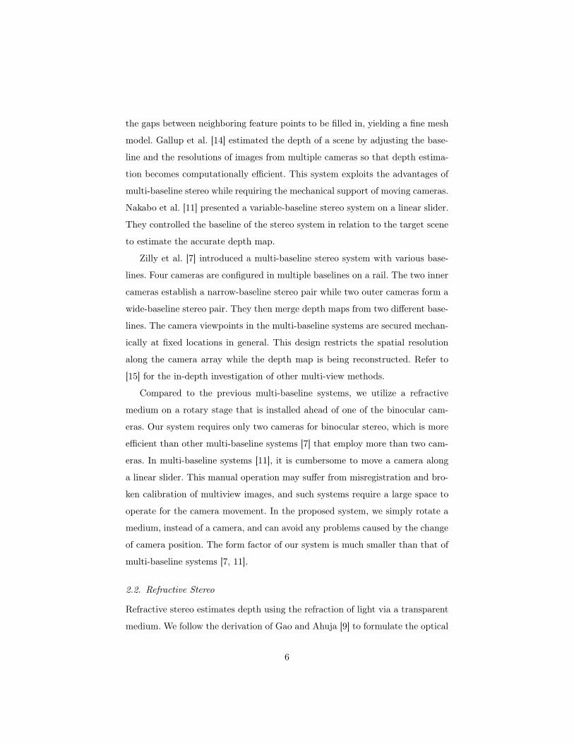
Compared to the previous multi-baseline systems, we utilize a refractive

medium on a rotary stage that is installed ahead of one of the binocular cam-

eras. Our system requires only two cameras for binocular stereo, which is more

efficient than other multi-baseline systems [7] that employ more than two cam-

eras. In multi-baseline systems [11], it is cumbersome to move a camera along

a linear slider. This manual operation may suffer from misregistration and bro-

ken calibration of multiview images, and such systems require a large space to

operate for the camera movement. In the proposed system, we simply rotate a

medium, instead of a camera, and can avoid any problems caused by the change

of camera position. The form factor of our system is much smaller than that of

multi-baseline systems [7, 11].

2.2. Refractive Stereo

Refractive stereo estimates depth using the refraction of light via a transparent

medium. We follow the derivation of Gao and Ahuja [9] to formulate the optical

6

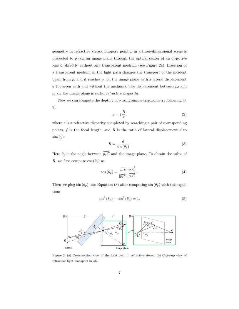
geometry in refractive stereo. Suppose point p in a three-dimensional scene is

projected to p

d

on an image plane through the optical center of an objective

lens C directly without any transparent medium (see Figure 2a). Insertion of

a transparent medium in the light path changes the transport of the incident

beam from p, and it reaches p

r

on the image plane with a lateral displacement

d (between with and without the medium). The displacement between p

d

and

p

r

on the image plane is called refractive disparity.

Now we can compute the depth z of p using simple trigonometry following [8,

9]:

z = f

R

r

, (2)

where r is a refractive disparity completed by searching a pair of corresponding

points, f is the focal length, and R is the ratio of lateral displacement d to

sin(✓

p

):

R =

d

sin (✓

p

)

. (3)

Here ✓

p

is the angle between−−!p

r

C and the image plane. To obtain the value of

R, we first compute cos (✓

p

) as

cos (✓

p

) =

−!p

r

e ·−−!pr

C

|−!pr

e|���−−!p

r

C

���. (4)

Then we plug sin (✓

p

) into Equation (3) after computing sin (✓

p

) with this equa-

tion:

sin

2(✓

p

) + cos

2(✓

p

) = 1. (5)

e

p

rp

dpCrt

R

z f

diθ pθ

Scene Image plane

Cedp

rp

Imageplane

r(a) (b)

iθ iθ

Figure 2: (a) Cross-section view of the light path in refractive stereo. (b) Close-up view of

refractive light transport in 3D.

7

Lateral displacement d, the parallel-shifted length of the light passing through

the medium, is determined as [16]

d =

1−

s1− sin

2(✓

i

)

n

2 − sin

2(✓

i

)

!t sin (✓

i

) , (6)

where t is the thickness of the medium, n is the refractive index of the medium,

and ✓

i

is the incident angle of the light. Here, sin (✓i

) can be obtained in a similar

manner as the case of sin (✓p

) using the following equation:

cos (✓

i

) =

−−!p

r

C ·−!eC���−−!p

r

C

������−!eC

���. (7)

The refracted point p

r

lies on a line, the so-called essential line, passing

through essential point e (an intersecting point of the normal vector of the

transparent medium to the image plane) and p

d

(see Figure 2b). This property

can be utilized to narrow down the search range of correspondences onto the

essential line, allowing us to compute matching costs efficiently. It is worth

noting that disparity in refractive stereo depends on not only the depth z of

p but also the projection position p

d

of light and the position of the essential

point e, whereas disparity in traditional stereo depends on only the depth z of

the point p. Before estimating a depth, we calibrate these optical properties in

refractive stereo in advance.

2.2.1. Refractive Stereo Approaches

Nishimoto and Shirai [17] first introduced a refractive camera system in which a

refractive medium is placed in front of a camera. Rather than computing depth

from refraction, their method estimates depth using a pair of a direct image

and a refracted one, assuming that the refracted image is equivalent to one

of the binocular stereo images. Lee and Kweon [18] presented a single camera

system that captures a stereo pair with a bi-prism. The bi-prism is installed in

front of the objective lens to separate the input image into a stereo pair with

refractive shift. The captured image includes a stereo image pair with a baseline.

Depth estimation is analogous to the traditional methods. Gao and Ahuja [8, 9]

8

proposed a seminal refractive stereo method that captures multiple refractive

images with a glass medium tilted at different angles. This method requires the

optical calibration of every pose of the medium. It was extended by placing a

glass medium on a rotary stage in [9]. The rotation axis of the tilted medium is

mechanically aligned to the optical axis of the camera. Although the mechanical

alignment is cumbersome, this method achieves more accurate depth than the

previous one does.

Shimizu and Okutomi [19, 20] introduced a mixed approach that combines

refraction and reflection phenomena. This method superposes a pair of reflection

and refraction images via the surface of a transparent medium. These overlap-

ping images are utilized as a pair of stereo images. Chen et al. [10, 21] proposed a

calibration method for refractive stereo. This method finds the pairs of matching

points on refractive images with the SIFT algorithm [22] to estimate the pose

of a transparent medium. They then search corresponding features using the

SIFT flow [23]. By estimating the rough scene depth, they recover the refractive

index of a transparent medium.

3. System Implementation

We propose a novel stereo fusion system that exploits the advantages of refrac-

tive and binocular stereo. This section describes technical details of the hardware

design and calibration methods for the proposed system.

3.1. Hardware Design

Our stereo fusion system consists of two cameras and a transparent medium

on a mechanical support structure. The focal length of both camera lenses is

8 mm. The cameras are placed on a rail in parallel with a baseline of 10 cm to

configure binocular stereo. We place a transparent medium on a rotary stage

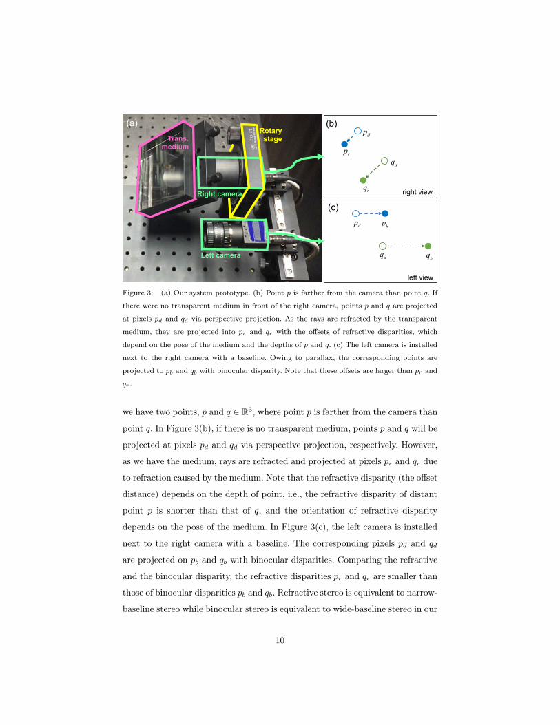
for refractive stereo in front of one of the binocular stereo cameras. Figure 3(a)

presents our system prototype. Figures 3(b) and (c) compare disparity changes

by the refractive medium (b) and the baseline in stereo (c), respectively. Suppose

9

Trans. medium

Rotary stage

Left camera

Right camera

dp

rpdq

rq

(a) (b)

(c)

dq qb

dp pb

right view

left view

Figure 3: (a) Our system prototype. (b) Point p is farther from the camera than point q. If

there were no transparent medium in front of the right camera, points p and q are projected

at pixels pd

and qd

via perspective projection. As the rays are refracted by the transparent

medium, they are projected into pr

and qr

with the offsets of refractive disparities, which

depend on the pose of the medium and the depths of p and q. (c) The left camera is installed

next to the right camera with a baseline. Owing to parallax, the corresponding points are

projected to pb

and qb

with binocular disparity. Note that these offsets are larger than pr

and

qr

.

we have two points, p and q 2 R3, where point p is farther from the camera than

point q. In Figure 3(b), if there is no transparent medium, points p and q will be

projected at pixels p

d

and q

d

via perspective projection, respectively. However,

as we have the medium, rays are refracted and projected at pixels pr

and q

r

due

to refraction caused by the medium. Note that the refractive disparity (the offset

distance) depends on the depth of point, i.e., the refractive disparity of distant

point p is shorter than that of q, and the orientation of refractive disparity

depends on the pose of the medium. In Figure 3(c), the left camera is installed

next to the right camera with a baseline. The corresponding pixels p

d

and q

d

are projected on p

b

and q

b

with binocular disparities. Comparing the refractive

and the binocular disparity, the refractive disparities pr

and q

r

are smaller than

those of binocular disparities pb

and q

b

. Refractive stereo is equivalent to narrow-

baseline stereo while binocular stereo is equivalent to wide-baseline stereo in our

10

system.

Our transparent medium is a block of clear glass. The measured refractive

index of the medium is 1.41 (⌘ = sin(20.00

◦)/ sin(14.04

◦)), and the thickness of

the medium is 28mm. We built a customized cylinder to hold the medium, cut

in 45◦ from the axis of the cylinder. The tilted medium spins around the optical

axis from 0◦ to 360◦ with angle intervals while capturing images. The binocular

stereo baseline and the tilted angle of the medium are fixed rigidly during image

capturing. For the input images of a scene, multiple images refracted by the

medium are captured on a camera and another image is obtained from the other

camera without the glass. Note that the refractive medium is not detached while

capturing the input.

3.2. Calibration

Our stereo fusion system requires several stages of prior calibration to estimate

depth information. This section summarizes our calibration processes.

3.2.1. Geometric Calibration

We first calibrate the extrinsic/intrinsic parameters of the cameras, including

the focal length of the objective lens, the center point of the image plane and

the lens distortion in order to convert the image coordinates into the global

coordinates. For the geometric calibration, we captured 14 different positions

on a chessboard. This allows us to derive an affine relationship between the

two cameras and rectify the coordinates of these cameras with respect to the

constraint epipolar line [24].

3.2.2. Refractive Calibration

Refractive stereo demands several optical calibrations related with the glass

medium, such as thickness, its refractive index, and the essential points of glass

orientation. This section presents our novel calibration method for refractive

stereo.

Analogous to the rectification of the epipolar line in binocular stereo, re-

fractive stereo requires calibration of the essential point e, where essential lines

11

Horizontal coordinate [px]180 200 220 240 260

Ver

tical

coo

rdin

ate

[px]

730

740

750

760

770

780

790

800

810

Horizontal coordinate [px]-2000 0 2000 4000

Ver

tical

coo

rdin

ate

[px]

-2000

-1000

0

1000

2000

3000

Direct point

(a) (b)

Refracted points

Angl

e of

the

med

ium

[deg

ree]

Image plane

Original essential points

50

100

150

200

250

300

350

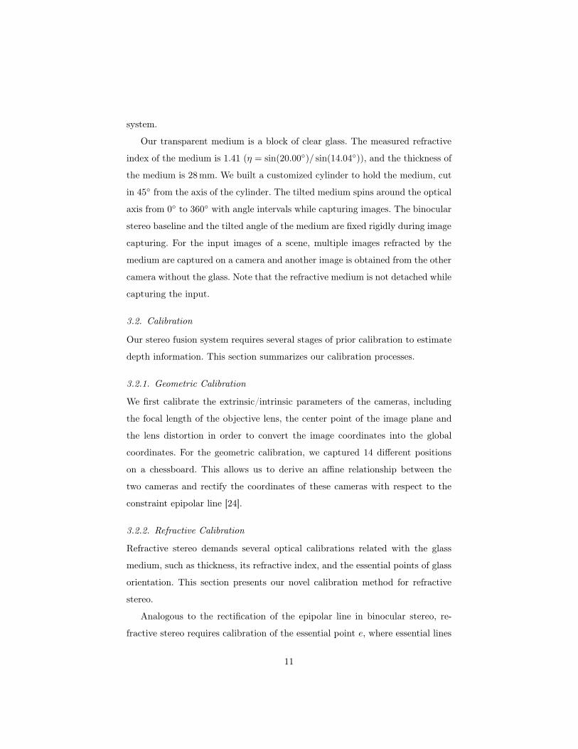
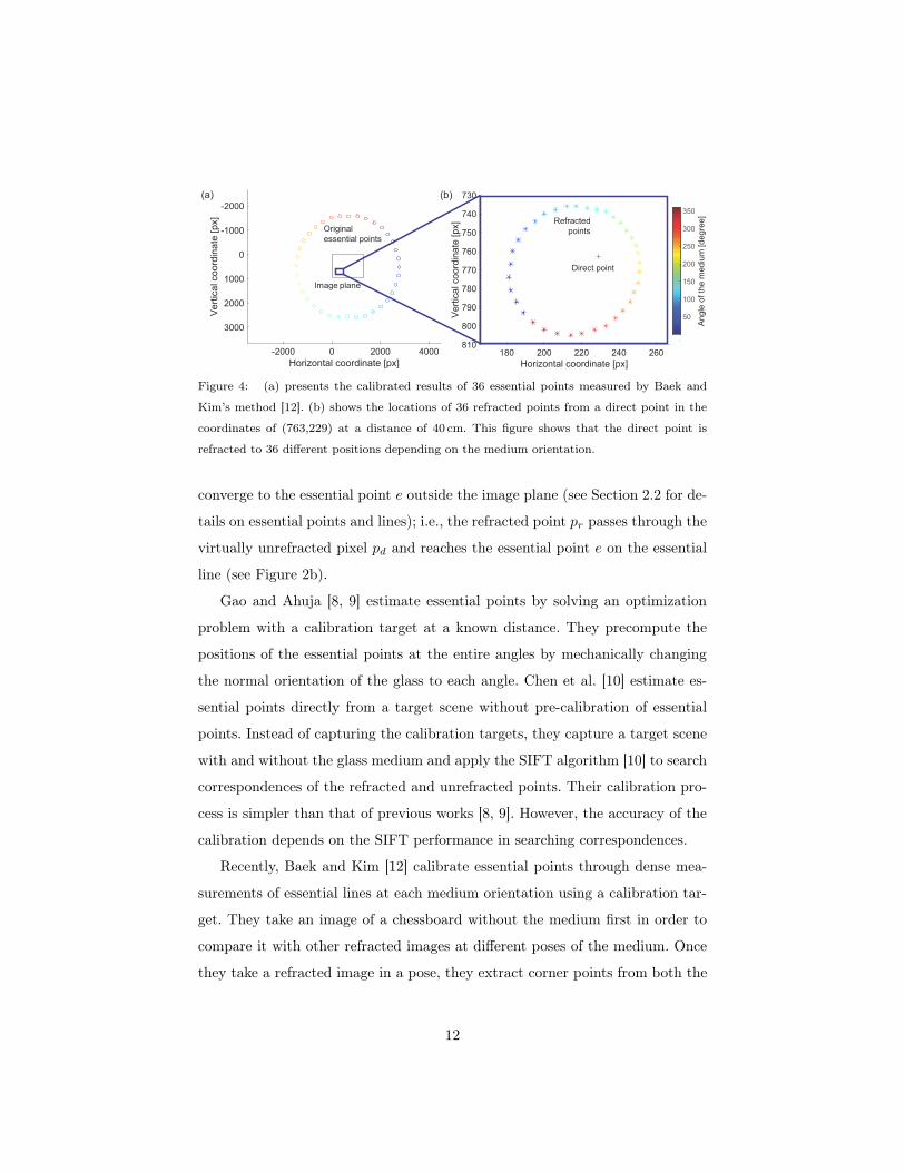
Figure 4: (a) presents the calibrated results of 36 essential points measured by Baek and

Kim’s method [12]. (b) shows the locations of 36 refracted points from a direct point in the

coordinates of (763,229) at a distance of 40 cm. This figure shows that the direct point is

refracted to 36 different positions depending on the medium orientation.

converge to the essential point e outside the image plane (see Section 2.2 for de-

tails on essential points and lines); i.e., the refracted point pr

passes through the

virtually unrefracted pixel pd

and reaches the essential point e on the essential

line (see Figure 2b).

Gao and Ahuja [8, 9] estimate essential points by solving an optimization

problem with a calibration target at a known distance. They precompute the

positions of the essential points at the entire angles by mechanically changing

the normal orientation of the glass to each angle. Chen et al. [10] estimate es-

sential points directly from a target scene without pre-calibration of essential

points. Instead of capturing the calibration targets, they capture a target scene

with and without the glass medium and apply the SIFT algorithm [10] to search

correspondences of the refracted and unrefracted points. Their calibration pro-

cess is simpler than that of previous works [8, 9]. However, the accuracy of the

calibration depends on the SIFT performance in searching correspondences.

Recently, Baek and Kim [12] calibrate essential points through dense mea-

surements of essential lines at each medium orientation using a calibration tar-

get. They take an image of a chessboard without the medium first in order to

compare it with other refracted images at different poses of the medium. Once

they take a refracted image in a pose, they extract corner points from both the

12

direct and the refracted images, where corresponding feature points appear at

different positions due to refraction. Superposing these two images, they draw

lines by connecting the corresponding points with all feature corners following

Chen et al. [10]. They then compute the arithmetic mean of the intersection

points’ coordinates to approximate essential point e

φ

per angle φ. They repeat

this process for every angle φ 2 Φ, where Φ is the set of angles for calibra-

tion. Figure 4(a) presents the calibrated essential points for Φ measured from

36 different orientations.

Whereas Gao and Ahuja [8, 9] require the measurement between the target

and the camera in addition to measuring essential lines, the method proposed

by Baek and Kim [12] does not require measurement of the distance from the

camera to the chessboard, and thus is more convenient. Note that Gao and

Ahuja [9] should capture four angles of the medium iteratively, until the rota-

tion axis of the medium meets the principal axis of the camera. Contrary to

Chen et al. [10], Baek and Kim [12] employ a calibration target to enhance

the reliability of refractive calibration. However, since their calibration requires

rigorous measurements of the entire angle variation, their measurement step

in refractive calibration is very cumbersome and introduces any measurement

errors.

In order to overcome the problem of cumbersome measurements in the cal-

ibration process, we propose a modified approach of the previous refractive

calibration introduced by Baek and Kim [12]. We were motivated to reduce

the number of per-angle measurements of correspondences while estimating the

entire essential points.

Euler Angle-Based Calibration. We propose a novel parametric approach of

refractive calibration on essential points. The key idea is to approximate the

entire essential points of every angle by using a parametric rotation of xyz-Euler

angles, where the rotation axis vector is optimized from a subset of measured

essential points.

Suppose we already estimated a certain number of essential points e

φ

for

13

sampled angles φ 2 Φ following Baek and Kim [12]. Let the rotation axis of the

medium be a unit vector u = [u

x

, u

y

, u

z

]

|, where kuk2 = 1. We denote the unit

normal vector of the medium at angle ' as n (') = [n

x

(') , n

y

(') , n

z

(')]

|,

where kn (')k2 = 1. Without loss of generality, we set the reference angle (one

of the measured angles) as zero degree. When we rotate the medium by degree '

from the reference angle with respect to the rotation axis u, the corresponding

normal vector n (') of the medium can be computed as follows:

n (') = T (',u)n (0) , (8)

where T (',u) is a rotation matrix that rotates a given vector n(0) by degree '

with respect to u. T (',u) is defined as an xyz-Euler angle rotation matrix with

a rotation axis u following [25]:

T (',u) =

2

6664

u

2x

v + c u

x

u

y

v − u

z

s u

x

u

z

v + u

y

s

u

y

u

x

v + u

z

s u

2y

v + c u

y

u

z

v − u

x

s

u

z

u

x

v − u

y

s u

z

u

y

v + u

x

s u

2z

v + c

3

7775, (9)

where c is defined as cos', s is sin', and v := 1− c.

e

C n

f

Imag

e pl

ane

e C

2

e Ce C

xyz

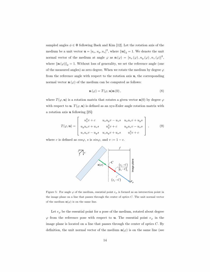
Figure 5: For angle ' of the medium, essential point e'

is formed as an intersection point in

the image plane on a line that passes through the center of optics C. The unit normal vector

of the medium n(') is on the same line.

Let e'

be the essential point for a pose of the medium, rotated about degree

' from the reference pose with respect to u. The essential point e

'

in the

image plane is located on a line that passes through the center of optics C. By

definition, the unit normal vector of the medium n(') is on the same line (see

14

Figure 5). We then formulate this relation between the essential point e

'

and

the normal n (') as follows:

n (') =

e

'

− C

ke'

− Ck2. (10)

We denote the right-hand side in Equation (10), (e

φ

− C)

�ke

φ

− Ck2, as

K

φ

. Our goal is to formulate essential points from any given angle rotation as a

parametric calibration model. This axis vector u and the reference normal n̂ (0)

satisfy Equations (8) and (10) from known values K

φ

and can be formulated as

an objective function:

min

u,n̂(0)

X

φ2

kT (φ,u) n̂ (0)−K

φ

k2 s.t. kn̂ (0)k2 = 1and kuk2 = 1, (11)

where n̂ (0) is the optimized reference normal of the medium. Note that it is

feasible to use n(0) directly instead of introducing n̂(0) using Equation (10).

However, we found that when one of direct measured normals is used as n(0)

in optimization of Equation (11), optimized essential points can be biased oc-

casionally upon an initial measurement error of n(0). We therefore choose to

apply a joint optimization approach to find both optimal n̂(0) and u in order

to enhance global accuracy.

We solve this non-linear objective function using a non-linear optimization

algorithm [26]. Note that we have six unknown variables of u and n̂(0). Since

the unit normal vector n(') has rank 2, Equation (11) gives us two equations

per angle φ. Therefore, we need at least three samples to solve Equation (11).

See Figure 12 for the impact of the number of input angles.

After optimizing u, we can compute the essential point e

'

at any arbitrary

angle ' of the medium. The essential point e'

is the intersection point of a line

that passes through the center of optic C displaced with f along the −z axis

(see Figure 5). Therefore, we can compute the essential point e

'

as follows:

e

'

=

T (',u) n̂ (0)

−T

z

(',u) n̂ (0)

f + C, (12)

where T

z

(',u) is the z-axis vector of T (',u).

15

In our experiment, we select a set of angles ⇥ to be used to estimate corre-

sponding essential points from the estimated u with Equation (8). We denote

the set of essential points as E for depth estimation.

3.2.3. Radiometric Calibration

Matching costs are calculated by comparing the intrinsic properties of color at

feature points. Since we attach a transparent medium on one of the stereo cam-

eras, it is critical to achieve consistent camera responses with and without the

medium. In our system, the right camera is attached with the glass medium

while the left camera is without any medium. We found that there are mis-

matches of colors captured in the same scene. We therefore characterize these

two cameras via radiometric calibration to match colors with each other. To do

this, we employed a GretagMacbeth ColorChecker target of 24 color patches.

We first captured an image from the refractive module with the medium and

an image from the other camera without the medium. Then, we linearized these

two RGB images with known gamma values as inverse gamma correction. Since

we had two sets of the linear RGB colors for the 24 patches, A and B (with

and without the medium), of which the dimensions were 24⇥ 3 each, we deter-

mined an affine transformation M of A to B as a camera calibration function

(a 3 ⇥ 3 matrix) using least-squares [27]. Once we characterized two camera

responses, we applied this color transform M for the linear RGB image which

was reconstructed from the images taken by the camera with the medium (see

Section 4.1.3). This color characterization allowed us to evaluate matching costs

for disparity through identical color reproductions of the two different cameras.

4. Depth Reconstruction in Stereo Fusion

Our stereo fusion workflow is composed of two stages. We first estimate an

intermediate depth map from a set of refractive stereo images (from the camera

with the refractive medium) and reconstruct a synthetic direct image. Then, this

virtual image and a direct image (from the other camera without the medium in

a baseline) are used to estimate the final depth map referring to the intermediate

16

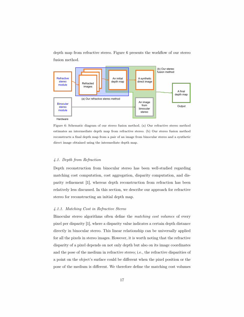
depth map from refractive stereo. Figure 6 presents the workflow of our stereo

fusion method.

Refracted images

A synthetic direct image Recover a

direct image

A final depth map

An image from

binocular stereo

Refractive stereo module

Binocular stereo module

An initial depth map

(a) Our refractive stereo method

(b) Our stereo fusion method

Hardware

Output

Figure 6: Schematic diagram of our stereo fusion method. (a) Our refractive stereo method

estimates an intermediate depth map from refractive stereo. (b) Our stereo fusion method

reconstructs a final depth map from a pair of an image from binocular stereo and a synthetic

direct image obtained using the intermediate depth map.

4.1. Depth from Refraction

Depth reconstruction from binocular stereo has been well-studied regarding

matching cost computation, cost aggregation, disparity computation, and dis-

parity refinement [1], whereas depth reconstruction from refraction has been

relatively less discussed. In this section, we describe our approach for refractive

stereo for reconstructing an initial depth map.

4.1.1. Matching Cost in Refractive Stereo

Binocular stereo algorithms often define the matching cost volumes of every

pixel per disparity [1], where a disparity value indicates a certain depth distance

directly in binocular stereo. This linear relationship can be universally applied

for all the pixels in stereo images. However, it is worth noting that the refractive

disparity of a pixel depends on not only depth but also on its image coordinates

and the pose of the medium in refractive stereo; i.e., the refractive disparities of

a point on the object’s surface could be different when the pixel position or the

pose of the medium is different. We therefore define the matching cost volumes

17

based on the depth, rather than the disparity, in our refractive stereo algorithm,

following a plane sweeping stereo method [28]. This approach allows us to apply

a cost volume approach for refractive stereo.

Suppose we have a geometric position set P of the refracted points pr

(p

d

, z, e)

of direct point p

d

at depth z (see Figure 2) with essential point e (e 2 E):

P (p

d

, z) = {pr

(p

d

, z, e)|e 2 E} . (13)

This set P can be derived analytically by refractive calibration (Section 3.2.2)

so that we precompute this set P for computational efficiency.

We denote L as the set of colors observed at the refracted positions P , where

l is a color vector in a linear RGB color space (l 2 L). Assuming that the surface

of the direct point p

d

is Lambertian, the colors of the refracted points L(p

d

, z)

would be the same. We use the similarity of L(pd

, z) for the matching cost C

of pd

with hypothetical depth z [29]. Note that our definition of the matching

cost is proportional to the similarity, different from the typical definition of the

matching cost in traditional stereo algorithms. The definition of the matching

cost is as follows:

C(p

d

, z) =

1

|L(pd

, z)|X

l2L(pd,z)

K(l − l). (14)

K is an Epanechnikov kernel [30] following:

K(l) =

8<

:1− kl/hk2, kl/hk 1

0, otherwise

, (15)

where h is a normalization constant (h = 0.01). Here, l is a mean color vector

of all elements in a set of L. We compute ¯

l with five iterations in L(p

d

, z) using

the mean shift method [31] as follows:

¯

l =

Pl2L(pd,z)

K(l − ¯

l)l

Pl2L(pd,z)

K(l − ¯

l)

. (16)

z in our refractive stereo is a discrete depth, the range of which is set between

60 cm and 120 cm at 3 cm intervals. Note that we build a refractive cost volume

per depth for all the pixels in the refractive image.

18

4.1.2. Cost Aggregation for Depth Estimation

To improve the spatial resolution of the intermediate depth map in refractive

stereo, we aggregate the refractive matching cost using a window kernel G.

Advanced cost aggregation techniques, such as guided image [32] and bi-

lateral weights [33], require a prior knowledge of the scene, i.e., a unrefracted

direct image. However, we do not capture the direct image in our experiments

because this requires detachment of the medium for every scene. Therefore, we

first aggregate the refractive matching costs using a Gaussian kernel G:

G(p

d

, q

d

) =

1

2⇡σ

2exp

✓−||p

d

− q

d

||2

2σ

2

◆, (17)

where σ is set to 9.6 as a parameter.

We filter the refractive matching cost at a pixel pd

in a depth z, where this

kernel convolves C(p

d

, z) with the matching costs of neighboring pixels with a

weighting factor G(p

d

, q

d

) [34]:

C

A

(p

d

, z) =

X

qd2w

G(p

d

, q

d

)C(q

d

, z), (18)

where q

d

is a pixel inside a squared window w, the size of which is 7⇥ 7.

Finally, we compute the optimal depth Z(p

d

) of the point pd

that maximizes

the aggregated matching costs:

Z(p

d

) = argmax

z

C

A

(p

d

, z). (19)

4.1.3. Reconstructing a Synthetic Direct Image

Even though the levels of the two cameras are the same on a rail as traditional

binocular stereo, our stereo pair includes more than horizontal parallax due

to the refraction effect. Prior to combining the estimated refractive depth and

the binocular stereo input, we reconstruct a synthetic image I

d

(a direct image

without the medium) by computing the mean radiance of the set L(p

d

, Z(p

d

))

using the mean shift method (Equation (16)). Note that this set L consists of

colors gathered from the refracted images.

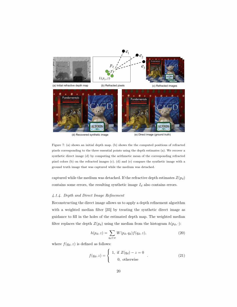
Figure 7 presents the initial depth map Z (a) and the reconstructed synthetic

direct image I

d

(d), which is compared with a ground truth image (e) that was

19

(a) Initial refractive depth map (c) Refracted images

(e) Direct image (ground truth)

dp 3e

2e1e

( , )dL p z

(b) Refracted pixels

(d) Recovered synthetic image

Figure 7: (a) shows an initial depth map. (b) shows the the computed positions of refracted

pixels corresponding to the three essential points using the depth estimates (a). We recover a

synthetic direct image (d) by computing the arithmetic mean of the corresponding refracted

pixel colors (b) on the refracted images (c). (d) and (e) compare the synthetic image with a

ground truth image that was captured while the medium was detached.

captured while the medium was detached. If the refractive depth estimates Z(p

d

)

contains some errors, the resulting synthetic image I

d

also contains errors.

4.1.4. Depth and Direct Image Refinement

Reconstructing the direct image allows us to apply a depth refinement algorithm

with a weighted median filter [35] by treating the synthetic direct image as

guidance to fill in the holes of the estimated depth map. The weighted median

filter replaces the depth Z(p

d

) using the median from the histogram h(p

d

, ·):

h(p

d

, z) =

X

qd2w

W (p

d

, q

d

)f(q

d

, z), (20)

where f(q

d

, z) is defined as follows:

f(q

d

, z) =

8<

:1, if Z(q

d

)− z = 0

0, otherwise

. (21)

20

Here, W is a weight function with a guided image filter [32], defined as

W (p

d

, q

d

) =

1

|w|2X

k:(pd,qd)2wk

(1 + (l

d

(p

d

)− µ

k

)(⌃

k

+ ✏U)

−1(l

d

(q

d

)−µ

k

)), (22)

where ld

(p

d

) is the linear RGB color of pd

on the direct image Id

, U is an identity

matrix, k is the center pixel of window w

k

including p

d

and q

d

, |w| is the number

of pixels in w

k

, and µ

k

and ⌃

k

are the mean vector and covariance matrix of Id

in w

k

. In our experiments, we set the size of wk

as 9⇥ 9, and we set ✏ as 0.001.

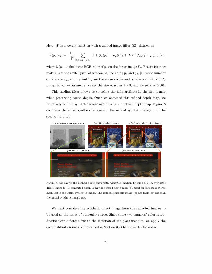
This median filter allows us to refine the hole artifacts in the depth map

while preserving sound depth. Once we obtained this refined depth map, we

iteratively build a synthetic image again using the refined depth map. Figure 8

compares the initial synthetic image and the refined synthetic image from the

second iteration.

(a) Refined refractive depth map (c) Refined synthetic direct image(b) Initial synthetic image

(d) Close-up view of (b) (e) Close up view of (c)

Figure 8: (a) shows the refined depth map with weighted median filtering [35]. A synthetic

direct image (c) is computed again using the refined depth map (a), used for binocular stereo

later. (b) is the initial synthetic image. The refined synthetic image (e) has more details than

the initial synthetic image (d).

We next complete the synthetic direct image from the refracted images to

be used as the input of binocular stereo. Since these two cameras’ color repro-

ductions are different due to the insertion of the glass medium, we apply the

color calibration matrix (described in Section 3.2) to the synthetic image.

21

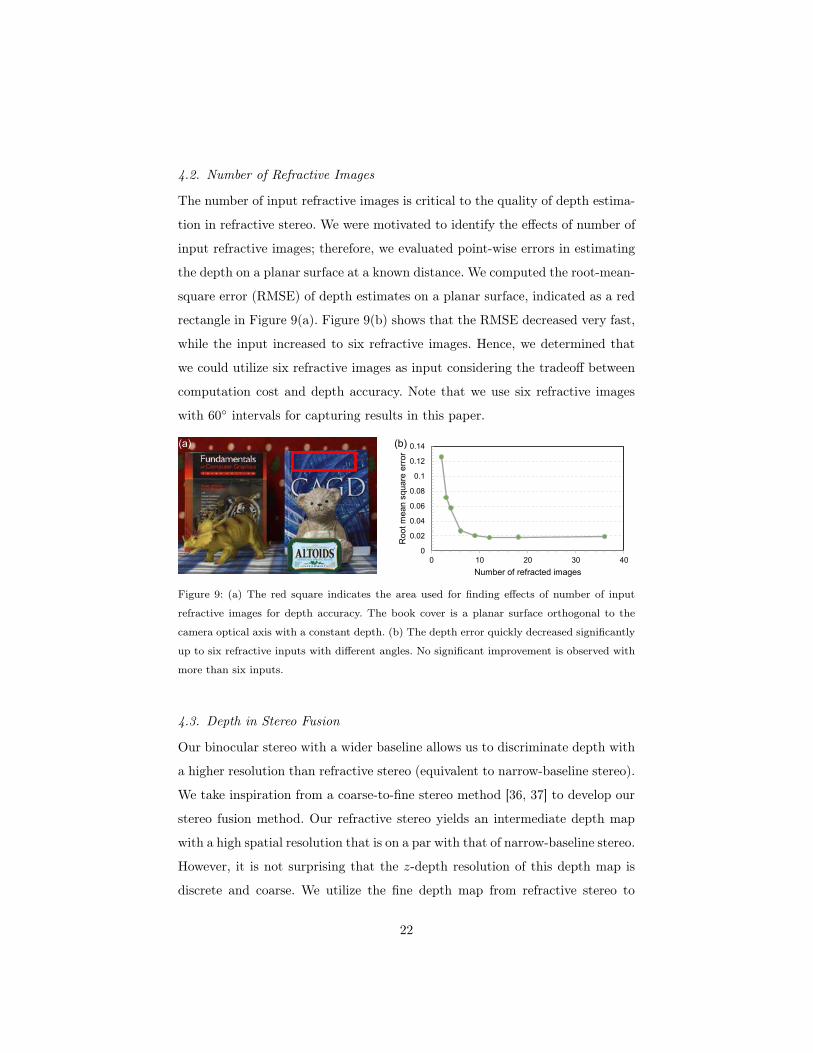
4.2. Number of Refractive Images

The number of input refractive images is critical to the quality of depth estima-

tion in refractive stereo. We were motivated to identify the effects of number of

input refractive images; therefore, we evaluated point-wise errors in estimating

the depth on a planar surface at a known distance. We computed the root-mean-

square error (RMSE) of depth estimates on a planar surface, indicated as a red

rectangle in Figure 9(a). Figure 9(b) shows that the RMSE decreased very fast,

while the input increased to six refractive images. Hence, we determined that

we could utilize six refractive images as input considering the tradeoff between

computation cost and depth accuracy. Note that we use six refractive images

with 60◦ intervals for capturing results in this paper.

0

0.02

0.04

0.06

0.08

0.1

0.12

0.14

0 10 20 30 40

Roo

t mea

n sq

uare

err

or

Number of refracted images

(b)(a)

Figure 9: (a) The red square indicates the area used for finding effects of number of input

refractive images for depth accuracy. The book cover is a planar surface orthogonal to the

camera optical axis with a constant depth. (b) The depth error quickly decreased significantly

up to six refractive inputs with different angles. No significant improvement is observed with

more than six inputs.

4.3. Depth in Stereo Fusion

Our binocular stereo with a wider baseline allows us to discriminate depth with

a higher resolution than refractive stereo (equivalent to narrow-baseline stereo).

We take inspiration from a coarse-to-fine stereo method [36, 37] to develop our

stereo fusion method. Our refractive stereo yields an intermediate depth map

with a high spatial resolution that is on a par with that of narrow-baseline stereo.

However, it is not surprising that the z-depth resolution of this depth map is

discrete and coarse. We utilize the fine depth map from refractive stereo to

22

increase the z-depth resolution as high as possible with a high spatial resolution

by limiting the search range of matching cost computation in binocular stereo

using the refractive depth map. To this end, we can significantly reduce the

chances of false matching while estimating depth from binocular stereo between

direct and synthetic images. This enables us to achieve a fine depth map from

binocular stereo, taking advantages of a high spatial resolution in refractive

stereo.

4.3.1. Matching Cost in Stereo Fusion

Now we have a direct image I

b

from the camera without the medium in the

binocular module and the synthetic image I

d

reconstructed from the refrac-

tive stereo module (Section 4.1.4) with its depth map. Depth candidates with

uniform intervals are not related linearly to the disparities with pixel-based in-

tervals. Hence, we define a cost volume for stereo fusion on the disparity instead

in order to fully utilize the image resolution. To fuse the depth from binocular

and refractive stereo, we build a fusion matching cost volume F (p

d

, d) per dis-

parity for all pixels as follows. The fusion matching cost F is defined as a norm

of the intensity difference:

F (p

d

, d) = kld

(p

d

)− l

b

(p

0d

)k , (23)

where p

0d

is a pixel shifted by a disparity d from p

d

, and l

b

(p

0d

) is a color vector

of p0d

on image I

b

.

4.3.2. Cost Aggregation in Stereo Fusion

In order to aggregate sparse matching costs, we first tried to use a guided image

filter that consists of multiple box filters, as done when refining refractive depth.

Prior to applying this filter, we reduce the search range of correspondence differ-

ently per each pixel using the depth map obtained from refractive stereo. Since

the guided filter exploits integral images, which need to be constructed for every

pixel and every depth candidate, its computational cost increases significantly

due to the wide range of valid depth candidates for high depth resolution. In-

stead of the guided filter, we use a bilateral filter W in Equation (24), as the

23

filter can be applied to the different ranges of depths per pixel independently.

We achieve a significant improvement in computational cost by applying the

bilateral image filter within a narrowed search range using the depth prior from

refractive stereo, while maintaining high depth resolution. The size of the kernel

w is 9⇥ 9, and the value of ✏ is 0.001 in our experiments. The aggregated cost

of the fusion matching costs in our method is defined as

F

A

(p

d

, d) =

X

qd2w

W (p

d

, q

d

)F (q

d

, d). (24)

Here W is the bilateral image filter [34] defined as

W (p

d

, q

d

) = exp

⇢−d(p

d

, q

d

)

σ

2s

− c(p

d

, q

d

)

σ

2c

�, (25)

where d(p

d

, q

d

) is the Euclidean distance between p

d

and q

d

, c(pd

, q

d

) is the sum

of differences of colors of RGB channels, and σ

s

and σ

c

are the standard devi-

ations for spatial distance and color difference, respectively. In our experiment,

we selected the window size, σs

, and σ

c

as 9, 7, and 0.07 respectively.

Suppose the depth of point p

d

is estimated as Z(p

d

) from refractive stereo.

As we compute the refractive matching cost and aggregate the cost per discrete

depth interval ∆z in refractive stereo, let the actual depth of p

d

be between

(Z(p

d

)−∆z) and (Z(p

d

) +∆z) as Z

prev

and Z

post

. The corresponding dispari-

ties of Zprev

and Z

post

can be computed as d

prev

and d

post

using Equation(1).

Note that dpost

is smaller than d

prev

. We therefore estimate the optimal dispar-

ity D(p

d

) by searching the aggregated cost volume F

A

(p

d

, d) within the range

[d

post

, d

prev

] as follows:

D(p

d

) = argmin

d

F

A

(p

d

, d). (26)

Note that we compute Equation (24) within the range of [dpost

, d

prev

] exclusively

for computational efficiency.

The ground true disparity of an orange pixel in Figure 10(a) is approxi-

mately 200. However, the disparity from binocular stereo was estimated as 160

because the minimum aggregated cost of binocular disparity has a local mini-

mum, yielding a wrong depth estimate. As a result, we were motivated to take

24

(a) Depth map from binocular stereo

(b) Depth map from our stereo fusion

0.00

0.05

0.10

0.15

0.20

0.25

0.30

142 152 162 172 182 192 202 212 222 232 242 252 262 272 282 292

Depth search range in our stereo fusion

Minimal cost in binocular stereo

Minimal cost in our stereo fusion

Aggr

egat

ed c

ost o

f dis

parit

y

Disparity (corresponding to the depth)

(c) Aggregated cost FA of disparity at pd=(339,213)

dpost dprev

Figure 10: The binocular depth map (a) includes artifacts due to false matching caused by

occlusions, featureless regions and repeated patterns. Using the intermediate refractive depth

map (b), we can limit the search range of a corresponding point pd

between dpost

and dprev

for instance. This significantly reduces false matching frequency in estimating depth.

a coarse-to-fine approach using both binocular and refractive disparity maps.

As shown in Figure 10(b), the refractive depth map tends to have fewer spa-

tial artifacts. We use this refractive disparity map as a guide map for searching

aggregated disparities. The search range is set to [d

post

, d

prev

] around the refrac-

tive depth estimate with a threshold. To this end, we are capable of preventing

faulty estimates in our stereo fusion.

5. Results

5.1. Implementations

We conducted several experiments to evaluate the performance of our stereo

fusion method. We computed depth maps, the resolution of which was 1280⇥960

with 140 depth steps, on a machine equipped with an Intel i7-3770 CPU and

16GB RAM with CPU parallelization. The computation times for estimating

the depth map from six refractive inputs was about 77 seconds for the first

stage of refractive stereo and about 33 seconds for the second-half stage of

stereo fusion. The total computation time on runtime is about 110 seconds

25

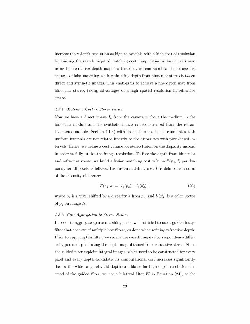
We precomputed the refracted essential points per pixel in the image plane

beforehand for computational efficiency.

(b) Refractive only stereo(a) Binocular only stereo (c) Our stereo fusion

Target

point

Binocular

only stereo

[mm]

Refractive

only stereo

[mm]

Our stereo

fusion

[mm]

Ground

truth [mm]

(i) 856 (+2) 863 (+9) 856 (+2) 854

(ii) 784 (+2) 784 (+2) 784 (+2) 782

(iii) 873 (+3) 863 (-7) 873 (+3) 870

(d)

Figure 11: The top rows compares the three different depth maps of binocular only stereo (a),

refractive only stereo (b) from the intermediate stage of our fusion method and our stereo

fusion (c) for a scene (d). Our stereo fusion method (c) does not suffer from false matchings

occurring at binocular only stereo (a). The bottom-right table presents the measured depth

values on three points in the scene, demonstrating that our method can discriminate close

surfaces, such as (i) and (iii), as much as binocular stereo does. Note that refractive stereo

cannot distinguish the depth differences between (i) and (iii).

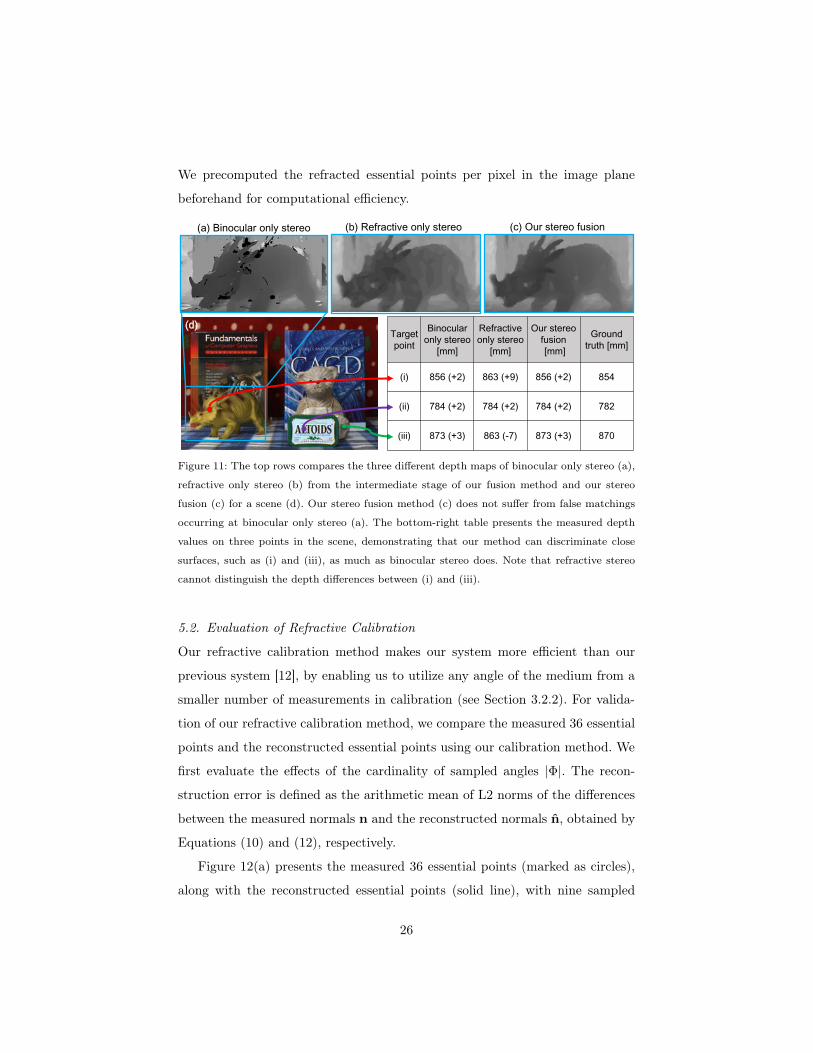
5.2. Evaluation of Refractive Calibration

Our refractive calibration method makes our system more efficient than our

previous system [12], by enabling us to utilize any angle of the medium from a

smaller number of measurements in calibration (see Section 3.2.2). For valida-

tion of our refractive calibration method, we compare the measured 36 essential

points and the reconstructed essential points using our calibration method. We

first evaluate the effects of the cardinality of sampled angles |Φ|. The recon-

struction error is defined as the arithmetic mean of L2 norms of the differences

between the measured normals n and the reconstructed normals n̂, obtained by

Equations (10) and (12), respectively.

Figure 12(a) presents the measured 36 essential points (marked as circles),

along with the reconstructed essential points (solid line), with nine sampled

26

angles (|Φ| = 9). Calibration error decreases rapidly up to nine samples, as

shown in Figure 12(b). We therefore chose nine angles for our calibration. We

estimate two depth maps (see Figures 12(c) and (d)): one from 36 measured

essential points, and the other from 36 reconstructed points, with calibration of

nine sampled angles.

Horizontal coordinate [px]-2000 0 2000 4000

Ver

tical

coo

rdin

ate

[px]

-2000

-1000

0

1000

2000

3000

Number of angle samples

0 10 20 30 40

Reconstr

uction e

rror

0.021

0.022

0.023

0.024

0.025

0.026

0.027

Image

plane

(a) (b)

Measured

essential points

Reconstructed

essential points

( )9Φ =

50

100

150

200

250

300

350

(c) (d)

Figure 12: (a) shows the measured essential points (circles), and the essential points (solid line)

calibrated from nine sampled angles. (b) describes the averaged calibration error of normals.

The calibration error decreases rapidly up to nine sampled angles. We therefore chose nine

angles for our calibration. (c) shows the refractive depth map obtained by 36 essential points

measured. We reconstruct a plausible depth map (d), with 36 reconstructed essential points,

obtained by nine sampled angles for calibration. Quantization artifacts shown in the depth

maps will be handled by our stereo fusion stage.

5.3. Quantitative Evaluation

The first row in Figure 11 compares three different depth maps obtained by

binocular only stereo (a), refractive only stereo (b) and our proposed stereo

fusion method (c). Although the depth estimation of binocular only stereo (a)

27

appears sound, (a) suffers from typical false matching artifacts around the edges

of the front object due to occlusion. Refractive only stereo (b), obtained from the

intermediate stage of our fusion method, presents depth without artifacts, but

the depth resolution is significantly discretized and coarse. Our stereo fusion (c)

overcomes the disadvantages of the homogeneous stereo methods. It estimates

depth as well as binocular stereo without severe artifacts.

We quantitatively evaluated the accuracy of our stereo fusion method in

comparison with the other methods in Figure 11(d). We measured three points

in the scene using a laser distance meter (Bosch GLM 80) and compared the

measurements by the three methods. The accuracy of our method is as high as

that of the binocular only method (averaged distance error: ⇠2 mm), while it is

superior to that of the refractive only method (aver. error: ⇠6 mm).

5.4. Qualitative Evaluation

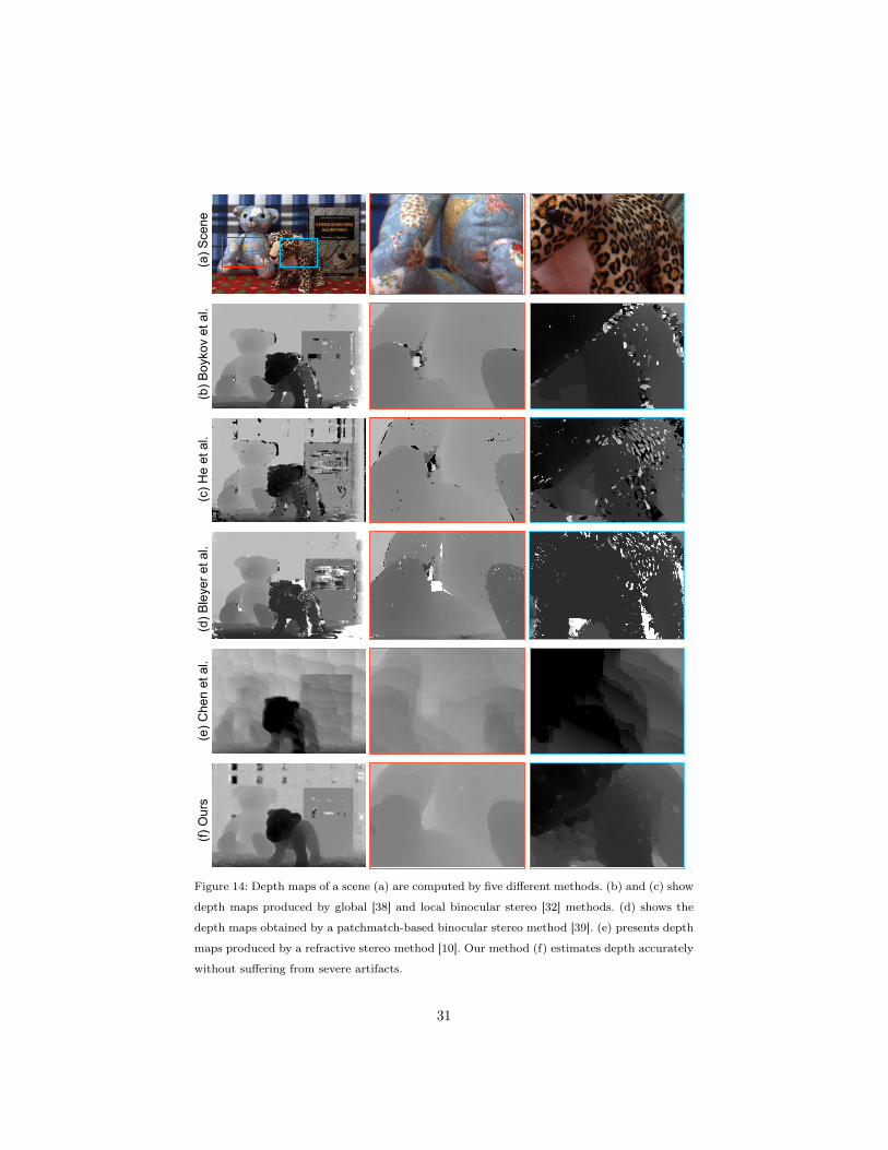
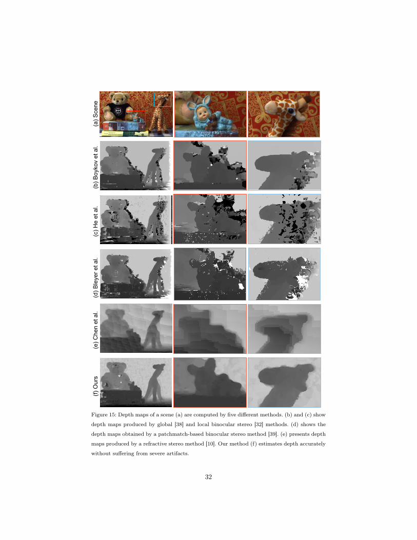
The first rows (a) in Figures 13, 14 and 15 present input images. The second

rows (b) in these figures are results of the graphcut-based method [38]. The

third rows (c) are results of a local binocular stereo method [32]. The fourth

rows present results of a patchmatch-based stereo method [39]. Note that we

utilize left and right images captured without any transparent medium as input

for the compared binocular stereo methods [38, 32, 39]. The fifth rows (e) show

results of a refractive stereo method [10]. The last rows (f) present results of

our stereo fusion method.

We compared our proposed method with a renowned graphcut-based al-

gorithm [38] with an image of the same resolution. Global stereo methods in

general allow for an accurate depth map, while requiring high computational

cost. It is not surprising that this global method was about eight times slower

than our method, although it produces an elaborate depth map.

We also compared our method with two local binocular methods [32, 39],

which compute matching cost as the norm of the intensity difference. In binocu-

lar methods [32, 39], the range of depth candidates is the same globally for every

pixel. He et al. [32] produce depth maps with some notable artifacts, and it took

28

about 212 seconds to compute, which is two times slower than our method. The

patchmatch-based stereo method [39] presents depth accuracy similar to that of

the graphcut-based algorithm [38]. It took about 720 seconds, which is slightly

faster than the graphcut-based method [38]. Thanks to the reduced range in

searching matching cost, our stereo fusion method outperforms other two lo-

cal stereo methods in terms of computational time, without sacrificing depth

accuracy.

A refractive method using SIFT flow [10] was also compared to ours. Six

refractive images were employed for both methods. While the refractive method

suffers from wavy artifacts caused by SIFT flow and its depth resolution is very

coarse, typical of refractive stereo, our method estimates depth accurately with

fewer spatial artifacts in all test scenes.

6. Future Work

Our hardware design requires at least one rotation of the medium to obtain a

depth map using more than two refracted images. The transparent medium was

manually rotated in our experiments. It restricts the applications of our system

to static scenes. Making the medium smaller and motorizing the rotation unit

to apply our system to dynamic scenes remains to be explored in our future

work.

Our pipeline currently consists of two stages: refractive depth estimation

and stereo fusion. As our stereo fusion follows a coarse-to-fine approach, errors

on the refractive depth map could be transferred to the final depth estimates.

In our future work, we would like to resolve this problem by accounting for

depth estimation and stereo fusion as a unified optimization problem to obtain

a high-fidelity depth map.

Since optical refraction is related with spectral dispersion, we would like

to apply our stereo fusion paradigm to hyperspectral imaging, exploiting re-

fraction effects on spectral dispersion. We anticipate that the combination of

hyperspectral imaging and refractive stereo imaging can broaden various fields

29

(e) C

hen

et a

l. (c

) He

et a

l. (b

) Boy

kov

et a

l. (a

) Sce

ne

(f) O

urs

(d) B

leye

r et a

l.

Figure 13: Depth maps of a scene (a) are computed by five different methods. (b) and (c) show

depth maps produced by global [38] and local binocular stereo [32] methods. (d) shows the

depth maps obtained by a patchmatch-based binocular stereo method [39]. (e) presents depth

maps produced by a refractive stereo method [10]. Our method (f) estimates depth accurately

without suffering from severe artifacts.30

(e) C

hen

et a

l. (c

) He

et a

l. (b

) Boy

kov

et a

l. (a

) Sce

ne

(f) O

urs

(d) B

leye

r et a

l.

Figure 14: Depth maps of a scene (a) are computed by five different methods. (b) and (c) show

depth maps produced by global [38] and local binocular stereo [32] methods. (d) shows the

depth maps obtained by a patchmatch-based binocular stereo method [39]. (e) presents depth

maps produced by a refractive stereo method [10]. Our method (f) estimates depth accurately

without suffering from severe artifacts.

31

(e) C

hen

et a

l. (c

) He

et a

l. (b

) Boy

kov

et a

l. (a

) Sce

ne

(f) O

urs

(d) B

leye

r et a

l.

Figure 15: Depth maps of a scene (a) are computed by five different methods. (b) and (c) show

depth maps produced by global [38] and local binocular stereo [32] methods. (d) shows the

depth maps obtained by a patchmatch-based binocular stereo method [39]. (e) presents depth

maps produced by a refractive stereo method [10]. Our method (f) estimates depth accurately

without suffering from severe artifacts.

32

of hyperspectral 3D imaging applications [40, 41, 42, 43].

7. Conclusions

We proposed a novel optical design combining binocular and refractive stereo

and introduced a stereo-fusion workflow. Our stereo fusion system is capable of

estimating depth information with a high depth resolution and fewer artifacts

at a speed that is competitive with other local and global binocular methods.

We validated that our proposed method combines the advantages of both tra-

ditional binocular and refractive stereo. Also, our refractive calibration method

makes our system more efficient than the previous method [12] by reducing the

calibration cost of refractive stereo. Our quantitative and qualitative evaluation

demonstrates that our fusion method outperforms the traditional homogeneous

methods in terms of artifacts and depth resolution. In addition to these ad-

vantages, our stereo fusion can be easily integrated into any existing binocular

stereo systems by simply introducing a transparent medium in front of a camera,

allowing for a significant improvement in a depth map with fewer artifacts.

Acknowledgements

Min H. Kim, the corresponding author, gratefully acknowledges Korea NRF

grants (2013R1A1A1010165 and 2013M3A6A6073718) and additional support

by an ICT R&D program of MSIP/IITP (10041313).

[1] D. Scharstein, R. Szeliski, A taxonomy and evaluation of dense two-frame

stereo correspondence algorithms, Int. J. Comput. Vision (IJCV) 47 (1-3)

(2002) 7–42.

[2] K. Kawashima, S. Kanai, H. Date, As-built modeling of piping system from

terrestrial laser-scanned point clouds using normal-based region growing,

J. Computational Design and Engineering 1 (1) (2014) 13–26.

[3] A. Kadambi, R. Whyte, A. Bhandari, L. V. Streeter, C. Barsi, A. A. Dor-

rington, R. Raskar, Coded time of flight cameras: sparse deconvolution

33

to address multipath interference and recover time profiles, ACM Trans.

Graphics (TOG) 32 (6) (2013) 167.

[4] A. Levin, R. Fergus, F. Durand, W. T. Freeman, Image and depth from a

conventional camera with a coded aperture, ACM Trans. Graphics (TOG)

26 (3) (2007) 70:1–9.

[5] C. Rhemann, A. Hosni, M. Bleyer, C. Rother, M. Gelautz, Fast cost-volume

filtering for visual correspondence and beyond, in: Proc. Computer Vision

and Pattern Recognition (CVPR), IEEE, 2011, pp. 3017–3024.

[6] M. Okutomi, T. Kanade, A multiple-baseline stereo, IEEE Trans. Pattern

Anal. Mach. Intell. (PAMI) 15 (4) (1993) 353–363.

[7] F. Zilly, C. Riechert, M. Müller, P. Eisert, T. Sikora, P. Kauff, Real-time

generation of multi-view video plus depth content using mixed narrow and

wide baseline, J. Visual Communication and Image Representation 25 (4)

(2013) 632–648.

[8] C. Gao, N. Ahuja, Single camera stereo using planar parallel plate, in: Proc.

Int. Conf. Pattern Recognition (ICPR), Vol. 4, 2004, pp. 108–111.

[9] C. Gao, N. Ahuja, A refractive camera for acquiring stereo and super-

resolution images, in: Proc. Comput. Vision and Pattern Recognition

(CVPR), 2006, pp. 2316–2323.

[10] Z. Chen, K.-Y. K. Wong, Y. Matsushita, X. Zhu, Depth from refraction

using a transparent medium with unknown pose and refractive index, Int.

J. Comput. Vision (ICJV) (2013) 1–15.

[11] Y. Nakabo, T. Mukai, Y. Hattori, Y. Takeuchi, N. Ohnishi, Variable base-

line stereo tracking vision system using high-speed linear slider, in: Proc.

Int. Conf. on Robotics and Automation (ICRA), 2005, pp. 1567–1572.

[12] S.-H. Baek, M. H. Kim, Stereo fusion using a refractive medium on a binoc-

ular base, in: Proc. Asian Conference on Computer Vision (ACCV 2014),

34

Vol. 9004 of Lecture Notes in Computer Science (LNCS), Springer, Singa-

pore, Singapore, 2015, pp. 503–518.

[13] Y. Furukawa, J. Ponce, Accurate, dense, and robust multiview stereopsis,

IEEE Trans. Pattern Anal. Mach. Intell. (PAMI) 32 (8) (2010) 1362–1376.

[14] D. Gallup, J.-M. Frahm, P. Mordohai, M. Pollefeys, Variable base-

line/resolution stereo, in: Proc. Comput. Vision and Pattern Recognition

(CVPR), 2008, pp. 1–8.

[15] S. M. Seitz, B. Curless, J. Diebel, D. Scharstein, R. Szeliski, A comparison

and evaluation of multi-view stereo reconstruction algorithms, in: Proc.

Comput. Vision and Pattern Recognition (CVPR), 2006, pp. 519–528.

[16] E. Hecht, Optics, Addison-Wesley, Reading, Mass, 1987.

[17] Y. Nishimoto, Y. Shirai, A feature-based stereo model using small dispari-

ties, in: Proc. Comput. Vision and Pattern Recognition (CVPR), 1987, pp.

192–196.

[18] D. Lee, I. Kweon, A novel stereo camera system by a biprism, IEEE Trans.

Robotics and Automation 16 (5) (2000) 528–541.

[19] M. Shimizu, M. Okutomi, Reflection stereo-novel monocular stereo using a

transparent plate, in: Proc. Canadian Conf. Computer and Robot Vision

(CRV), IEEE, 2006, pp. 14–14.

[20] M. Shimizu, M. Okutomi, Monocular range estimation through a double-

sided half-mirror plate, in: Proc. Canadian Conf. Computer and Robot

Vision (CRV), IEEE, 2007, pp. 347–354.

[21] Z. Chen, K. Wong, Y. Matsushita, X. Zhu, M. Liu, Self-calibrating depth

from refraction, in: Proc. Int. Conf. Comput. Vision (ICCV), 2011, pp.

635–642.

[22] D. G. Lowe, Distinctive image features from scale-invariant keypoints, Int.

J. Comput. Vision (IJCV) 60 (2) (2004) 91–110.

35

[23] C. Liu, J. Yuen, A. Torralba, Sift flow: Dense correspondence across scenes

and its applications, Pattern Analysis and Machine Intelligence, IEEE

Transactions on 33 (5) (2011) 978–994.

[24] Z. Zhang, A flexible new technique for camera calibration, IEEE Trans.

Pattern Anal. Mach. Intell. (PAMI) 22 (11) (2000) 1330–1334.

[25] S. J. Gortler, Foundations of 3D computer graphics, MIT Press, London,

2012.

[26] R. A. Waltz, J. L. Morales, J. Nocedal, D. Orban, An interior algorithm

for nonlinear optimization that combines line search and trust region steps,

Mathematical Programming 107 (3) (2006) 391–408.

[27] M. H. Kim, J. Kautz, Characterization for high dynamic range imaging,

Computer Graphics Forum (Proc. EUROGRAPHICS 2008) 27 (2) (2008)

691–697.

[28] R. T. Collins, A space-sweep approach to true multi-image matching, in:

Computer Vision and Pattern Recognition, 1996. Proceedings CVPR’96,

1996 IEEE Computer Society Conference on, IEEE, 1996, pp. 358–363.

[29] C. Kim, H. Zimmer, Y. Pritch, A. Sorkine-Hornung, M. Gross, Scene re-

construction from high spatio-angular resolution light fields, ACM Trans.

Graph. (TOG) 32 (4) (2013) 73:1–12.

[30] R. O. Duda, P. E. Hart, Pattern Classification and Scene Analysis, Wiley,

1973.

[31] D. Comaniciu, P. Meer, Mean shift: A robust approach toward feature

space analysis, IEEE Trans. Pattern Anal. Mach. Intell. (PAMI) 24 (5)

(2002) 603–619.

[32] K. He, J. Sun, X. Tang, Guided image filtering, in: Proc. European Con-

ference on Computer Vision (ECCV), Springer, 2010, pp. 1–14.

36

[33] S. Mattoccia, S. Giardino, A. Gambini, Accurate and efficient cost aggre-

gation strategy for stereo correspondence based on approximated joint bi-

lateral filtering, in: Proc. Asian Conference on Computer Vision (ACCV),

Springer, 2010, pp. 371–380.

[34] K.-J. Yoon, I. S. Kweon, Adaptive support-weight approach for correspon-

dence search, IEEE Trans. Pattern Anal. Mach. Intell. (PAMI) 28 (4) (2006)

650–656.

[35] Z. Ma, K. He, Y. Wei, J. Sun, E. Wu, Constant time weighted median

filtering for stereo matching and beyond, in: Proc. Int. Conf. Computer

Vision (ICCV), 2013, pp. 1–8.

[36] S. T. Barnard, Stochastic stereo matching over scale, Int. J. Comput. Vision

(IJCV) 3 (1) (1989) 17–32.

[37] J.-S. Chen, G. Medioni, Parallel multiscale stereo matching using adaptive

smoothing, in: Proc. European Conference on Computer Vision (ECCV),

1990, pp. 99–103.

[38] Y. Boykov, O. Veksler, R. Zabih, Fast approximate energy minimization

via graph cuts, IEEE Trans. Pattern Anal. Mach. Intell. (PAMI) 23 (11)

(2001) 1222–1239.

[39] M. Bleyer, C. Rhemann, C. Rother, Patchmatch stereo-stereo matching

with slanted support windows., in: BMVC, Vol. 11, 2011, pp. 1–11.

[40] G. Nam, M. H. Kim, Multispectral photometric stereo for acquiring high-

fidelity surface normals, IEEE Computer Graphics and Applications 34 (6)

(2014) 57–68.

[41] H. Lee, M. H. Kim, Building a two-way hyperspectral imaging system with

liquid crystal tunable filters, in: Proc. Int. Conf. Image and Signal Process-

ing (ICISP) 2014, Lecture Notes in Computer Science, Vol. 8509, Springer,

Normandy, France, 2014, pp. 26–34.

37

[42] M. H. Kim, T. A. Harvey, D. S. Kittle, H. Rushmeier, J. Dorsey, R. O.

Prum, D. J. Brady, 3D imaging spectroscopy for measuring hyperspectral

patterns on solid objects, ACM Trans. Graph. (Proc. SIGGRAPH 2014)

31 (4) (2012) 38:1–11.

[43] M. H. Kim, H. Rushmeier, J. ffrench, I. Passeri, D. Tidmarsh, Hyper3d: 3d

graphics software for examining cultural artifacts, ACM Journal on Com-

puting and Cultural Heritage 7 (3) (2014) 1:1–19.

38