Embed Size (px)
Citation preview

Stiffness and Capacity of
Foundations on Layered Clays
October 2018
This thesis is submitted for the degree of Master of Civil Engineering of the University of Western Australia Faculty of Engineering and Mathematical Sciences
Yishan Tian

Abstract This paper presents the laboratory results for the ultimate bearing capacity for layered clays. The clays
consist of a thin layer of stiff crust lying over a thick layer of soft clay which are both consolidated
from the same batch of kaolin mix. The two samples were consolidated under different pressure to
achieve different undrain shear strength and were compiled thereafter. Aluminium footings with
diameter 20, 40, 60 and 80mm were utilized respectively to verify the correlation between footing
diameter and depth of the stiff soil. To obtain the soils’ undrain shear strength value, CPT and T-bar
tests were conducted respectively. The experiment data was compared with the result from predictions
from previous studies results conducted by Brown & Meyerhof and Merifield and finite element
simulation using Plaxis.

Contents Abstract ................................................................................................................................................... 0
1. Introduction ..................................................................................................................................... 4
2. Literature review ............................................................................................................................. 5
3. Experiment ...................................................................................................................................... 6
3.1 Overview ....................................................................................................................................... 6
3.2 Experiment premise and assumed model ...................................................................................... 6
3.3 Experimental Apparatus and preparation ...................................................................................... 6
3.3.1 Chamber ................................................................................................................................. 6
3.3.2 Footings .................................................................................................................................. 6
3.3.3 Actuator .................................................................................................................................. 7
3.3.4 Evacuation Auger ................................................................................................................... 7
3.3.5 Sample consolidation ............................................................................................................. 9
3.3.6 Soil transportation ................................................................................................................ 11
3.4 Experiment procedure ................................................................................................................. 12
3.5 Soil profile result ......................................................................................................................... 12
3.6 Conducted experiment ................................................................................................................ 13
4. Data Comparison .......................................................................................................................... 15
4.1 Experiment data process ............................................................................................................. 15
4.1.1 The isotropic linear elastic perfectly plastic model .............................................................. 17
4.1.2 Comparison between the experiment data with the Mohr-Coulomb model ........................ 18
4.1.3 The change of Nc factor with respect of H/B ...................................................................... 20
5. Compare the measured capacity with predictions from previous theories .................................... 23
5.1 Brown and Meyerhof’s Method .............................................................................................. 23
5.2 Merifield’s table ...................................................................................................................... 23
6. Numerical analysis ........................................................................................................................ 25
6.1 Model construction ..................................................................................................................... 25
6.1.1 Initial soil model .................................................................................................................. 25
6.1.2Structural Restriction ............................................................................................................ 25
6.1.3 Select mesh resolution ......................................................................................................... 26
6.1.4 Stage construction ................................................................................................................ 27
6.2 Result comparison ....................................................................................................................... 27
7. Conclusion .................................................................................................................................... 33
Reference .............................................................................................................................................. 34
Appendix ............................................................................................................................................... 36

Before everything starts, allow me to express my gratitude to my supervisor Professor Barry Lehane,
who has assisted me with my experiment and research throughout the past year. The same thanks go
to Dr. Qingbing Liu who has given me a great deal of help academically. The experiment was
prepared in the civil lab in UWA and it couldn’t be done without the help from Mr. Jim Waters.
Special thanks go to Mr. Manuel Palacios who not only created and printed the evacuation ring,
which is the coolest part of this experiment and taught me how to use the actuator as well so I am
able to conduct the experiment.
Finally, I’d like to thank my parents who have supported me both financially and mentally. I couldn’t
have done it without them. The past five years has not always been easy, but fortunately it is coming
to an end.
That’s probably enough digression for now, let’s begin.

1. IntroductionThe theory of continental drift was proposed by Alfred Wegener in 1912, which was able to explain
crustal movement from ancient time. Although seems motionless, the soil moves slowly but
persistently since the beginning of time. The tectonic movement caused volcano, earthquake and other
geological instabilities, which resulted in soil not being uniform (Wegener, 1966). Layered soil is
extremely common under natural condition. A layer of weak soil underlying a layer of think crust is a
common situation due to its universality and unpredictable nature. The ultimate bearing capacity is
reached when the contribution of the soft clay is completely incorporated, the failure in such a pattern
is denoted punching failure since the top layer was punched into the bottom layer. (Brown&
Meyerhof, 1969)
Over the past few decades, extensive studies were conducted on the subject of bearing capacity on
layered clays. However due to the complication of creating such two-layered soil sample artificially,
almost all researches are conducted by finite element analysis method. The two widely recognized
experiments-based researches are conducted by Brown and Meyerhof in 1969 using both circular and
strip footings and Merifield’s rigorous plasticity solution in 1999. It was proposed in both papers that
the ultimate bearing capacity has a relationship with the thickness of the upper crust and the
respective undrained shear strength of the two layers.
The intention of this report is to ascertain what would the actual bearing capacity of the layered clay
be and how does the result compare to the previous developed solution and the finite element analysis.
The experiment was used kaolin mix as the material both the top crust and the bottom layer, which
can both be classified as undrained. Each of the layers possesses relatively uniform properties that
was consolidated separately to achieve different undrained shear strength. Smooth circular aluminium
footings were utilized during the experiment to avoid undesirable effect to the result.

2. Literature reviewThe bearing capacity factor was first proposed by Terzaghi in 1943 and was studied on widely after
that. As the researches on the subject of single layered soil have matured, geotechnical engineers have
the opportunity to study the response of non-homogeneous soil when loaded by a foundation, which is
more realistic as it resembles the real-life soil condition.
The subject of two-layered clay was first touched by Button in 1953, he determined an upper bound
solution by assuming a circular failure mode. The same failure mechanism was later adopted by
Reddy and Sirnivasan (1967) for another upper bound solution by using limit equilibrium. Another
study by Chen in 1975 was conducted and a sequential formula was derived on the subject by
assuming a similar circular rupture failure. However, the three methodologies were criticized by
Davis and Booker (1973) due to the overestimation of the bearing capacity.
Based on experiment results, a semi-empirical solution was developed by Brown and Meyerhof (1969)
and an empirical solution by Meyerhof and Hanna (1975). Since these two methods were based on
experimental results rather than finite element analysis, they were used as guidelines to be studied and
compared by all the researches carried after them. Which would also be used to compare with the
experiment result in this report.
Merifield et al. (1999) developed rigorous plasticity solutions for bearing capacity of layered clays
based on the finite element analysis by Sloan (1988) and Sloan and Kleeman (1995). Goss and
Griffiths (2001) adopted a small displacement FE analysis which allows Zhu and Michalowski (2005)
and Merifield and Nguyen (2006) to utilize the same method to conduct extensive studies on various
shapes of foundations. Wang and Carter (2002) and Yu et al. (2011) used large deformation finite
element analysis to run the estimation of layered soil’s bearing capacity.
The all the studies conducted in the past two decades on this subject are solely based on finite element
analysis. While the advantage of such method is obvious, which is easy to conduct and the extinction
of possible mistake, there could be some unknown interaction between the layered soil that could not
possibly beknown to mathematical matrices. The reliability of FE analysis needs to be further
analysed.
Four previously obtained solutions were studied in this report and compared with the experiment
result, including: the semi-empirical and empirical solution developed respectively by Brown&
Meyerhof and Meyerhof& Hannah, Meyerhof’s rigorous plasticity solution and Chen’s upper bound
circular shaped failure.
3. Experiment
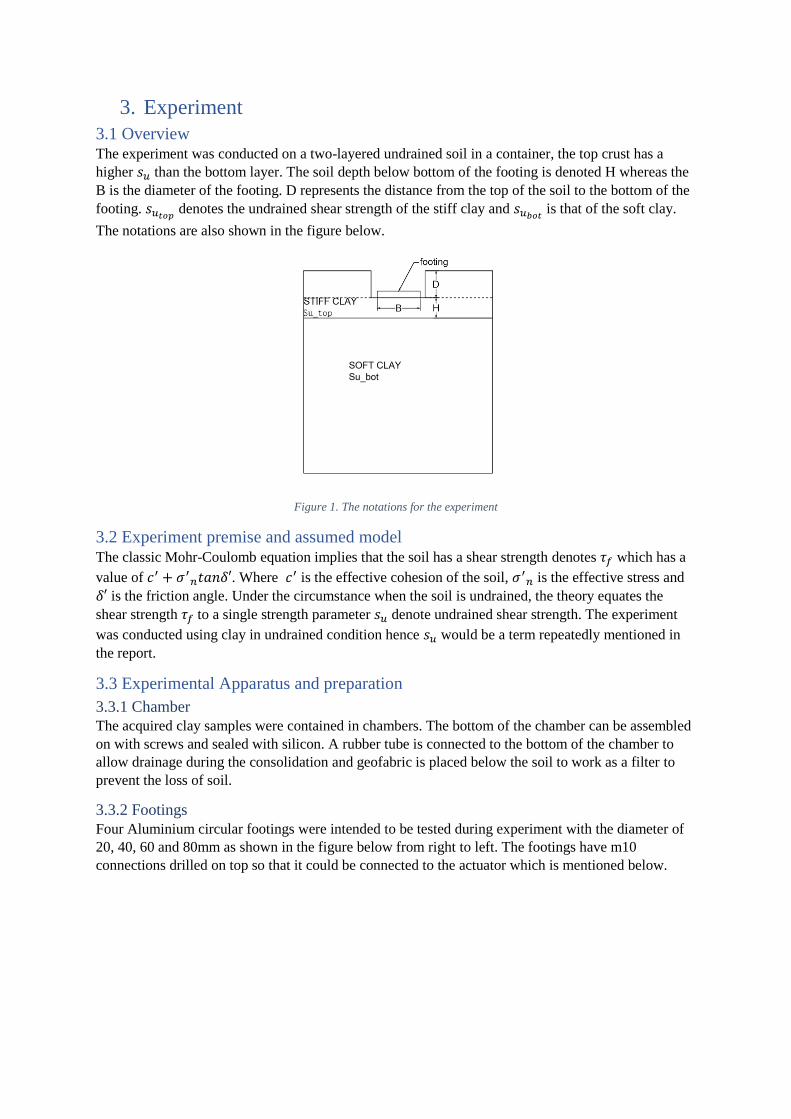
3.1 Overview The experiment was conducted on a two-layered undrained soil in a container, the top crust has a
higher 𝑠𝑢 than the bottom layer. The soil depth below bottom of the footing is denoted H whereas the
B is the diameter of the footing. D represents the distance from the top of the soil to the bottom of the
footing. 𝑠𝑢𝑡𝑜𝑝 denotes the undrained shear strength of the stiff clay and 𝑠𝑢𝑏𝑜𝑡
is that of the soft clay.
The notations are also shown in the figure below.
Figure 1. The notations for the experiment
3.2 Experiment premise and assumed model The classic Mohr-Coulomb equation implies that the soil has a shear strength denotes 𝜏𝑓 which has a
value of 𝑐′ + 𝜎′𝑛𝑡𝑎𝑛𝛿′. Where 𝑐′ is the effective cohesion of the soil, 𝜎′
𝑛 is the effective stress and
𝛿′ is the friction angle. Under the circumstance when the soil is undrained, the theory equates the
shear strength 𝜏𝑓 to a single strength parameter 𝑠𝑢 denote undrained shear strength. The experiment
was conducted using clay in undrained condition hence 𝑠𝑢 would be a term repeatedly mentioned in
the report.
3.3 Experimental Apparatus and preparation
3.3.1 Chamber
The acquired clay samples were contained in chambers. The bottom of the chamber can be assembled
on with screws and sealed with silicon. A rubber tube is connected to the bottom of the chamber to
allow drainage during the consolidation and geofabric is placed below the soil to work as a filter to
prevent the loss of soil.
3.3.2 Footings
Four Aluminium circular footings were intended to be tested during experiment with the diameter of
20, 40, 60 and 80mm as shown in the figure below from right to left. The footings have m10
connections drilled on top so that it could be connected to the actuator which is mentioned below.

Figure 2. The foundations tested with a diameter of 20, 40, 60 and 80mm (from right to left)
3.3.3 Actuator
To measure the force and displacement provided on the footing, an actuator is required, which is
shown in Figure 3 below. The actuator has two axis which enables it to move both horizontally and
vertically, two output slots were connected to the computer. It was clamped onto the chamber for
steadiness. The computer can control and read the displacement of the actuator. An extension rod is
supposed to be fixed along the actuator and connect both the footing and a load cell which was also
plugged into a computer.
Figure 3. The actuator used in the experiment.
3.3.4 Evacuation Auger
The layered clays were consolidated under high pressure to achieve a certain value of undrained shear
strength which would be absent just before and during the experiment. This would cause the very top
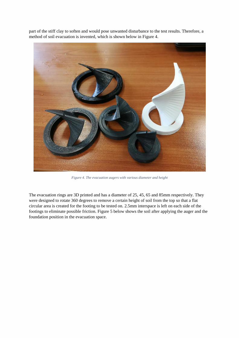
part of the stiff clay to soften and would pose unwanted disturbance to the test results. Therefore, a
method of soil evacuation is invented, which is shown below in Figure 4.
Figure 4. The evacuation augers with various diameter and height
The evacuation rings are 3D printed and has a diameter of 25, 45, 65 and 85mm respectively. They
were designed to rotate 360 degrees to remove a certain height of soil from the top so that a flat
circular area is created for the footing to be tested on. 2.5mm interspace is left on each side of the
footings to eliminate possible friction. Figure 5 below shows the soil after applying the auger and the
foundation position in the evacuation space.

Figure 5a (on the left). The soil appearance after having applied the auger.
Figure 5b (on the right). the position of the footing relative to the evacuation space.
3.3.5 Sample consolidation
The two kaolin mix samples were acquired fully saturated and with 120% water content, is intended
to be consolidated separately to achieve different undrained shear strength. The samples were
contained in chambers and were pressed using the lever arm system shown in the figure below. The
intended stiff crust is to be consolidated under a pressure up to 200kPa whereas the intended soft clay
would be consolidated under 32kPa.
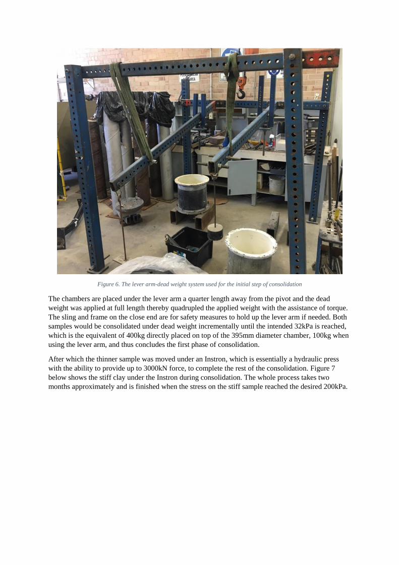
Figure 6. The lever arm-dead weight system used for the initial step of consolidation
The chambers are placed under the lever arm a quarter length away from the pivot and the dead
weight was applied at full length thereby quadrupled the applied weight with the assistance of torque.
The sling and frame on the close end are for safety measures to hold up the lever arm if needed. Both
samples would be consolidated under dead weight incrementally until the intended 32kPa is reached,
which is the equivalent of 400kg directly placed on top of the 395mm diameter chamber, 100kg when
using the lever arm, and thus concludes the first phase of consolidation.
After which the thinner sample was moved under an Instron, which is essentially a hydraulic press
with the ability to provide up to 3000kN force, to complete the rest of the consolidation. Figure 7
below shows the stiff clay under the Instron during consolidation. The whole process takes two
months approximately and is finished when the stress on the stiff sample reached the desired 200kPa.

Figure 7. Stiff clay consolidated under the Instron
3.3.6 Soil transportation
After having the two soil samples ready separately, the stiff clay needs to be transferred onto the soft
clay to complete the layered clay configuration. However this posed a certain conundrum regarding
the soil transfer. The stiff clay cannot be direct drop on top of the soft clay since that might cause
cracks and thus compromise the integrity of the clay which is extremely undesirable.
The method developed was exploiting the cohesion between the cap of the chamber and the soil. The
cap, which could also be referred to as the platen, is utilized to bear the pressure and apply it
uniformly onto the soil. The bottom of the chamber can be removed after untightening the screws
from the chamber. The stiff clay can be pushed out of the chamber by putting weight onto the platen
while the chamber was lifted by a crane. The set up can be observed in the figures below.
Figure 8a (on the left) shows the set up during the soil transfer.
Figure 8b (on the right) shows the soil after it was pushed out.

As shown on Figure 8a, the soil was gently pushed out by the weight on the platen, below which is
foam covered with black plastic to mitigate the possible dropping. Figure 8b shows the shape of the
stiff clay after it was pushed out. Since the air is depleted between the interface of the soil and the
platen, the stiff clay can be lifted by the handles and placed on to the soft clay. To remove the platen
from the soil, a thin steel wire is applied to cleave the soil thus complete the process of soil transfer.
The compiled soil was subsequently consolidated under 32kPa again for compaction, after which the
soil would be ready for the experiment.
3.4 Experiment procedure The experiment set up is shown in the figure below.
Figure 9a. The actuator used in the experiment.
Figure 9b. The extention rod with load cell connected to the footing.
The actuator was clamped onto the chamber for steadiness and the extension rod with the footing and
load cell shown in Figure 9b which would be connected to the actuator. After which the footing can
be controlled by the actuator to load the layered soils. CPT and T-bar tests were conducted first to
obtain the undrained shear strength profile of the compiled soil.
Soil was evacuated using the printed auger before each footing test was conducted. The footing
moved downward at the speed of 0.01mm/s and stoped after having reached a total of 20% of its
diameter to reach the soil’s ultimate bearing capacity and the corresponding load was recorded and
transferred back to the computer.
3.5 Soil profile result Two sets of experiments were conducted over the time of two semesters with different properties. The
two sets of experiments, denote EXP01 and EXP02, have the 𝑠𝑢 profile illustrated in Figure 10 below.
From the results from the soil property test, a best estimated 𝑠𝑢 value is given for each experiment as
the theoretical number used in the calculation.

Figure 10. The CPT and T-bar result and best estimation for Su for EXP01&02.
The stiff soil’s thickness was 74mm for EXP01 and has an undrained shear strength of 15.3kPa
whereas that of the soft soil is 7.4kPa. For EXP02, the layered soil has a Su value of 20kPa and 4kPa
respectively and the thickness of the stiff clay is 108mm. The information gathered from the CPT and
T-bar tests indicated that the top crust is about twice as stiff as the soft layer for EXP01 whereas for
EXP02 it is five times. The soil properties are summarized in the table below.
Table 1. The summarized soil properties for the two experiments
Thickness for stiff soil
(mm) 𝑠𝑢,𝑡𝑜𝑝 for stiff soil
(kPa)
𝑠𝑢,𝑏𝑜𝑡 for soft soil
(kPa)
𝑠𝑢,𝑡𝑜𝑝
𝑠𝑢,𝑏𝑜𝑡 ratio
EXP01 74 15.3 7.4 2.07
EXP02 108 20 4 5
3.6 Conducted experiment Three footings tests were conducted during EXP01 using 40,60 and 80mm foundation while the auger
applied has the depth of 32mm, which leaves a H value of 42mm.
For EXP02, all four footings were tested with the 32mm auger. After which the 40mm footings were
test separately with an evacuation depth of 80mm and again directly on the soft clay.
The table below contains the list of all the tests and the regarding parameters.
-200
-150
-100
-50
0
0 10 20 30 40
De
pth
(m
m)
Su (kPa)EXP02
CPT01 CPT02 best estimate Su profile-140
-120
-100
-80
-60
-40
-20
0
0 10 20 30 40
Dep
th (
mm
)
su (kPa)
EXP01
Tbar4
CPT01
CPT02
Best estimate su profile
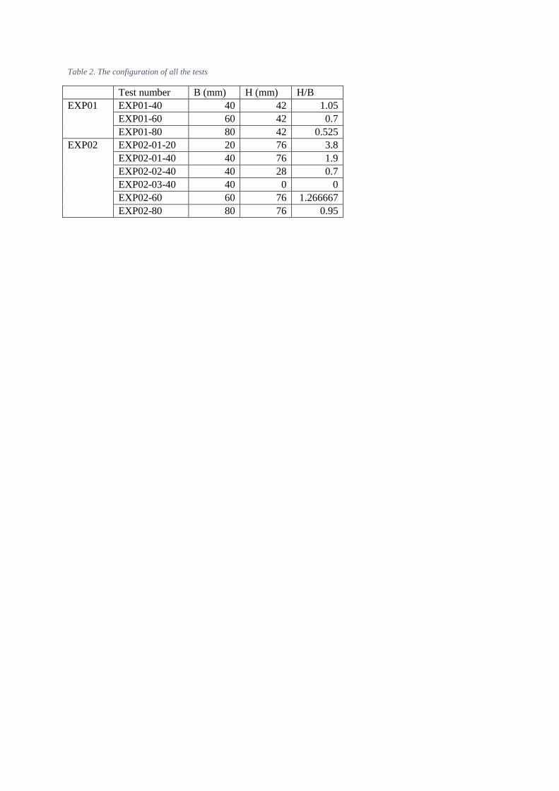
Table 2. The configuration of all the tests
Test number B (mm) H (mm) H/B
EXP01 EXP01-40 40 42 1.05
EXP01-60 60 42 0.7
EXP01-80 80 42 0.525
EXP02 EXP02-01-20 20 76 3.8
EXP02-01-40 40 76 1.9
EXP02-02-40 40 28 0.7
EXP02-03-40 40 0 0
EXP02-60 60 76 1.266667
EXP02-80 80 76 0.95

4. Data Comparison
4.1 Experiment data process The original feedback direct from the computer has two entries, the displacement and the force. The
force can be converted to pressure by dividing the respective area of the footing and the displacement
is divided by the diameter to a dimensionless term s/B. Plot the pressure against s/B. Figure 11 shows
the plot for EXP01-80.
Figure 11. The raw data for EXP01-80
The orange line is the unprocessed raw data. Due to the nature of model experiment, the measurement
taken at the start of each test was not accurate. Adhering to the principle of retaining as much real data
as possible, the initial part of the data is ignored and extrapolated by the rest of the data. After which
the starting point of the plot is moved to the origin depicted by the blue line. The same process is done
for all the tests and is shown in the figure below.
0
10
20
30
40
50
60
70
80
90
100
0 0.05 0.1 0.15 0.2 0.25
q/k
Pa
s/B
test data
test data

Figure 12. The experiment data for EXP01
Figure 13. The experiment data for EXP02
0
20
40
60
80
100
120
140
0 0.05 0.1 0.15 0.2 0.25
q (
kPa)
s/B
Plot for EXP01
EXP01-60
EXP01-80
EXP01-40
0
50
100
150
200
250
0 0.02 0.04 0.06 0.08 0.1 0.12 0.14 0.16 0.18 0.2
q (
kPa)
s/B
Plot for EXP02
EXP02-01-20 EXP02-01-40 EXP02-60 EXP02-80 EXP02-03-40 EXP02-02-40

4.1.1 The isotropic linear elastic perfectly plastic model
An important point cannot be stress enough in soil mechanics is that, soil is not a elastic material.
However, for the purpose of studying soil, the soil properties have to be put in the form of numbers
for the soil to be able to be studied. The Mohr-Coulomb circle is a theory that was recognized
universally in the geotechnics community, which is displayed in the figure below.
Figure 14. The soil property relationship for the soil’s Mohr Coulomb circle.
The Mohr-Coulomb soil model is idealized to go through completely linear elastic at first and
becomes entirely plastic after reached a turning point. (Lehane, 2017) The model can also be referred
to as the isotropic linear elastic perfectly plastic model for soil. The idealized stress-strain curve for
undrained soil is shown in the figure below.

Figure 15. The idealized stress-strain curve for undrained soil under Mohr-Coulomb Model. (Lehane, 2017)
According to this model, the initial part of the line depends directly on the soil’s Elastic modulus and
the elastic limit is reached when the stress increases to the value of 2𝑠𝑢.
4.1.2 Comparison between the experiment data with the Mohr-Coulomb model
As it can be observed from Figure 12 and Figure 13, the shape of the curves is analogous to the plot
shown in Figure 15, even though the real soil is not perfectly linear elastic- plastic, the gradient hardly
changes at the beginning of the test and then gradually decreases to zero. Hence, the stress-strain
curve for the layered soil is the same as isotropic soil, the initial part of the test data is directly related
to the Modulus of the soil, and the bearing capacity depends on the undrained shear stress.
Another key observation can be made from Figure 13 is that the initial gradient is almost identical for
H/B>0.95 (EXP02-20, EXP02-01-40, EXP02-60 and EXP02-80), for Figure 12 as well. The smaller
the value of H/B is, the sooner the gradient reduces. The explanation can be made is that the
foundation is only affected by the upper layer of stiff clay at first, but as the foundation was pushed
deeper, the threshold of no soft clay influence was crossed, then the soft clay contributes to the
bearing capacity and hence the gradient becomes smaller. In the extreme case of H/B=0, indicating
the nonexistence of stiff clay, the bearing capacity would be depended entirely on the soft clay, hence
there is no coincide of soil stiffness whatsoever with the rest of the experiment data.
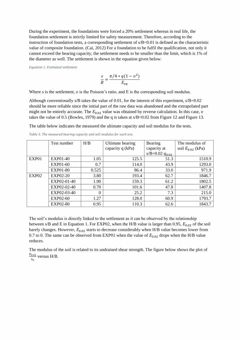
During the experiment, the foundations were forced a 20% settlement whereas in real life, the
foundation settlement is strictly limited for safety measurement. Therefore, according to the
instruction of foundation tests, a corresponding settlement of s/B=0.01 is defined as the characteristic
value of composite foundation. (Cai, 2012) For a foundation to be fulfil the qualification, not only it
cannot exceed the bearing capacity, the settlement needs to be smaller than the limit, which is 1% of
the diameter as well. The settlement is shown in the equation given below:
Equation 1. Estimated settlement
𝑠
𝐵=
𝜋 4⁄ ∗ 𝑞(1 − 𝜐2)
𝐸𝑒𝑞
Where s is the settlement, 𝜐 is the Poisson’s ratio, and E is the corresponding soil modulus.
Although conventionally s/B takes the value of 0.01, for the interest of this experiment, s/B=0.02
should be more reliable since the initial part of the raw data was abandoned and the extrapolated part
might not be entirely accurate. The 𝐸0.02 value was obtained by reverse calculation. In this case, 𝜐takes the value of 0.5 (Bowles, 1979) and the q is taken at s/B=0.02 from Figure 12 and Figure 13.
The table below indicates the measured the ultimate capacity and soil modulus for the tests.
Table 3. The measured bearing capacity and soil modulus for each test.
Test number H/B Ultimate bearing
capacity q (kPa)
Bearing
capacity at
s/B=0.02 𝑞0.02
The modulus of
soil 𝐸0.02 (kPa)
EXP01 EXP01-40 1.05 125.5 51.3 1510.9
EXP01-60 0.7 114.0 43.9 1293.0
EXP01-80 0.525 86.4 33.0 971.9
EXP02 EXP02-20 3.80 193.4 62.7 1846.7
EXP02-01-40 1.90 159.3 61.2 1802.5
EXP02-02-40 0.70 101.6 47.8 1407.8
EXP02-03-40 0 25.2 7.3 215.0
EXP02-60 1.27 128.0 60.9 1793.7
EXP02-80 0.95 110.3 62.6 1843.7
The soil’s modulus is directly linked to the settlement as it can be observed by the relationship
between s/B and E in Equation 1. For EXP02, when the H/B value is larger than 0.95, 𝐸0.02 of the soil
barely changes. However, 𝐸0.02 starts to decrease considerably when H/B value becomes lower from
0.7 to 0. The same can be observed from EXP01 when the value of 𝐸0.02 drops when the H/B value
reduces.
The modulus of the soil is related to its undrained shear strength. The figure below shows the plot of 𝐸0.02
𝑠𝑢 versus H/B.

Figure 16. The plot of E/Su versus H/B
From Figure 16, it could be postulated that when H/B exceeds 0.95, the equivalent soil modulus
remains the same however big H/B is. However, when H/B is smaller than 0.95, the equivalent soil
modulus is affected by the H/B value. This postulate is of significant meaning if it were true. A
relationship between H/B and E can be established thus the prediction accuracy for settlement on
layered soil would be increased drastically. Due to the limitation of time and resources, the data point
obtained is not enough to depict the relationship between 𝐸0.02
𝑠𝑢 and H/B.
An assumption could be made here is that they have a linear relationship before H/B=0.95, after
which 𝐸0.02
𝑠𝑢 remains the same as the line drawn in Figure 16 indicates.
Also, it could be observed that the value of 𝐸0.02
𝑠𝑢 for both EXP01 and EXP02 is around the value of 95,
after E0.02 was fully developed.
4.1.3 The change of Nc factor with respect of H/B
The comprehensive bearing capacity theory was initially proposed by Karl von Terzaghi which given
the bearing capacity factor 𝑁𝑐 a value of 5.14 for undrained soil. (Terzaghi, 1943). The general
bearing capacity theory for the undrained case is shown as Equation 2 below:
Equation 2. General bearing capacity theory for undrained soil (Lehane, 2017)
𝑞𝑓 = 𝑁𝑐𝑠𝑐𝑑𝑐𝑖𝑐𝑠𝑢
Where 𝑠𝑐 is the shape factor and has the value of 1.2 for circular footing.
𝑑𝑐 is the depth factor and 𝑖𝑐 is the inclination factor which has the value of one for vertical load.
Equation 3. The determination of the depth factor dc (Lehane, 2017)
𝑑𝑐 = 1 + 0.4 (𝐷
𝐵) 𝑓𝑜𝑟
𝐷
𝐵< 1
𝑑𝑐 = 1 + 0.4𝑡𝑎𝑛−1 (𝐷
𝐵) 𝑓𝑜𝑟
𝐷
𝐵> 1
0
20
40
60
80
100
120
0 0.5 1 1.5 2 2.5 3 3.5 4
𝐸0
.02
/S𝑢
_to
p
H/B
E/Su_top versus H/B
EXP01
EXP02

However, the value of 𝑁𝑐 factor is not constantly 5.14. In the case of inhomogeneous soil, 𝑁𝑐 factor
was the main focus of study. The ultimate bearing capacity could be determined by using 𝑁𝑐 times the
undrained shear strength for the stiff clay.
Use the bearing capacity obtained from the experiment to reverse calculate the value of 𝑁𝑐 for each
test. The table and figure below present all the tests and their corresponding 𝑁𝑐.
Table 4. The back calculated Nc factor corresponding to each test
Test number H/B Ultimate
bearing
capacity q
(kPa)
𝑠𝑢_𝑡𝑜𝑝 Foundation
depth D
(mm)
Depth
factor 𝑑𝑐
Bearing
capacity
factor 𝑁𝑐
EXP01-40 1.05 125.5 15.3 32 1.32 5.18
EXP01-60 0.7 114.0 15.3 32 1.21 5.13
EXP01-80 0.525 86.4 15.3 32 1.16 4.06
EXP02-20 3.80 193.4 20 32 1.64 4.91
EXP02-01-40 1.90 159.3 20 32 1.32 5.03
EXP02-02-40 0.70 101.6 20 80 1.80 2.35
EXP02-03-40 0 25.2 4 (no stiff
clay)
108 2.08 2.52
EXP02-60 1.27 128.0 20 32 1.21 4.41
EXP02-80 0.95 110.3 20 32 1.16 3.96
Figure 17. Plot the back calculated Nc versus H/B for each test
Though there are only three measurement points from EXP01, the trend can be unequivocally
observed. The Nc factor increases with the increment of H/B until it reaches the maximum value of
approximately 5.14 for circular footings. (Bienen, 2018)
0
1
2
3
4
5
6
0 0.5 1 1.5 2 2.5 3 3.5 4
Nc
fact
or
H/B
Nc versus H/B
EXP01 Su ratio=2.07
EXP02 Su ratio=5

Another observation could be made based on the plot is that for EXP01, the Nc factor reaches 5.14
sooner than EXP02. The Su ratio for EXP01 is much larger than EXP02, which means the soft clay in
EXP01 is stiffer than the soft clay in EXP02. Therefore, EXP02 is relatively more sensitive to the
ratio of H/B. The Nc value reached its limit when H/B is around 1.7 for EXP01, whereas for EXP02,
Nc’s maximum is reached when H/B is only 0.7. The larger the Su ratio is, the larger H/B must be for
Nc to become maximum.
The conclusion that can be drawn is that, for fixed 𝑠𝑢𝑡𝑜𝑝
𝑠𝑢𝑏𝑜𝑡
value, Nc factor increases when H/B
increases until Nc reaches 5.14. The larger 𝑠𝑢𝑡𝑜𝑝
𝑠𝑢𝑏𝑜𝑡
is, the larger H/B has to be for Nc to reaches its
maximum. This coincides with the findings from Brown& Meyerhof, Meyerhof& Hanna, Chen and
Merifield. In the next section, the experiment results would be used to compared with all those
aforementioned previous studies’ predictions.
5. Compare the measured capacity with predictions from previous
theories
5.1 Brown and Meyerhof’s Method
The analytical equation developed by Brown and Meyerhof is
Equation 4. Equation developed by Brown& Meyerhof (1969)
𝑁𝑐 =3𝐻
𝐵+
6.05𝑠𝑢𝑏𝑜𝑡
𝑠𝑢𝑡𝑜𝑝
The equation can only be used to predict the circumstance of a punching failure.
Calculate the bearing capacity factor using Equation 4 for each test and compare the value with the 𝑁𝑐
from the experiment.
Table 5. Comparison between the measured capacity and Brown& Meyerhof's prediction
Test number H/B Bearing capacity
factor 𝑁𝑐
𝑁𝑐 Predicted using
Equation 4
Error percentage (%)
EXP01-40 1.05 5.18 6.08 17.37
EXP01-60 0.7 5.13 5.03 1.95
EXP01-80 0.525 4.06 4.5 10.84
EXP02-20 3.80 4.91 12.61 (not applicable) -
EXP02-01-40 1.90 5.03 6.91 37.38
EXP02-02-40 0.70 2.35 3.31 40.85
EXP02-03-40 0 2.52 1.21 (not applicable) -
EXP02-60 1.27 4.41 5.02 13.83
EXP02-80 0.95 3.96 4.06 2.53
Compare the experiment data to the prediction, Brown& Meyerhof’s formula generally overestimate
which is mentioned in the paper. Some of the prediction is quite accurate with the error around 10%.
Other estimation, however, were not satisfactory.
The study was conducted and published in the 1960s. The precision of the apparatus has enhanced
substantially during the past few decades. Now that the failure capacity can be more accurately
detected, the prediction made by an equation developed over half a century ago naturally becomes
inadequate. However, Brown& Meyerhof’s method was certainly ahead of its time and still is
mentioned, cited and compared to as a guideline for the layered clay studies.
For EXP02-01-20 and EXP02-03-40, the two-layered clay punching shear model was not applicable.
The stiff clay was too thick hence the top crust was not punched through for the former and no
presence of the top crust for the latter.
5.2 Merifield’s table
A rigorous solution for two-layered clays’ bearing capacity was developed by Merifield, Sloan and
Yu. They have compared the Nc factor they derived with others. The number were provided and
compared with the previous result from the experiment in the table below. The original table from the
paper is attached in the appendix in Figure 29 and Figure 30.

Table 6. Compare the obtained value with three other predictions
Test number Bearing
capacity
factor
Merifield
et al
Chen,
1975
Meyerhof&
Hanna, 1978
EXP01-40 5.18 4.63 5.11 4.46
EXP01-60 5.13 4.18 4.43 3.99
EXP01-80 4.06 3.7 3.94 3.51
EXP02-20 4.91 - - -
EXP02-01-40 5.03 4.96 5.53 4.2
EXP02-02-40 2.35 2.71 3.13 2.14
EXP02-03-40 2.52 - - -
EXP02-60 4.41 3.8 4.58 3.05
EXP02-80 3.96 3.22 3.75 2.54
Combine Table 5 and Table 6 together, the Nc value from the experiment and the prediction of the
other four studies is shown in the table below for a better comparison.
Table 7. The compiled Nc factor table from the experiment and four previous studies.
Test number Bearing
capacity
factor
Merifield
et al,
1999
Chen,
1975
Meyerhof&
Hanna, 1978
Brown &
Meyerhof, 1969
EXP01-40 5.18 4.63 5.11 4.46 6.08
EXP01-60 5.13 4.18 4.43 3.99 5.03
EXP01-80 4.06 3.7 3.94 3.51 4.5
EXP02-20 4.91 - - - -
EXP02-01-40 5.03 4.96 5.53 4.2 6.91
EXP02-02-40 2.35 2.71 3.13 2.14 3.31
EXP02-03-40 2.52 - - - -
EXP02-60 4.41 3.8 4.58 3.05 5.02
EXP02-80 3.96 3.22 3.75 2.54 4.06
Compare between the three previous studies, Chen’s prediction is the most accurate, Merifield’s
method is the second. Meyerhof & Hanna’s method shows a gross underestimation across the board,
whereas Brown& Meyerhof’s method shows a certain amount of overestimation generally.
All the studies made the assumption that the stiff soil went through punching failure and general
failure was fully developed at the bottom layer. Such a failure pattern would occur when H/B is
smaller than 2 (Meyerhof et al, 1999), hence the test EXP02-01-20 does not fulfil this requirement.

6. Numerical analysis To simulate the exact condition and soil parameter in the experiment, soil mechanics analyse software
Plaxis were used to run the FE analysis. The identical experimental procedure and soil properties were
input into the software.
6.1 Model construction
6.1.1 Initial soil model
First a borehole needs to be created to construct the soil body. In the software, a layer of stiff clay on
the top and another layer of soft clay was created where the Mohr-Coulomb model is selected. Soil
parameters, such as unit weight, Young’s Modulus and undrained shear strength, were entered, and
the soil body constructed is shown in the figure below. The blue block represents the stiff clay
whereas the pink block is the soft clay.
Figure 18. The soil model created in the software.
The axis-symmetry option was selected for the model, which means the actual soil volume created in
the software is symmetrical around the y-axis. Therefore, the soil model actually constructed in the
software is twice as big as presented in Figure 18.
6.1.2Structural Restriction
Certain restriction conditions have to be input to prevent the soil from prematurely collapse and the
soil evacuation depth needs to be defined afterwards. The appearance of the model is shown in Figure
19 below.

Figure 19. The soil model after having defined the boundary condition and evacuation depth.
The rectangular on the top left corner of Figure 19 is the prepared position for the footing. The soil on
the left boundary of the model is only allowed to move vertically, close to where the footings was
supposed to be put in afterwards, the horizontal movement is restricted which results in the several
sets of short parallel green lines. The soil on the right boundary and at the bottom was forbade to
undergo any movement whatsoever since they are too far away from the footing, hence the green
pound signs.
6.1.3 Select mesh resolution
The soil model was completed regarding soil structure. The model needs to be meshed like any FE
analysis and the calculation can be conducted afterwards. The mesh of the model is shown in the
figure below.
Figure 20. The fraction of the soil model meshed.

There are five rectangles in Figure 20 are shown in the colour green which are the regions that were
meshed. It is important to mesh the region that are of interest in Plaxis since it would be extremely
time consuming when the whole model was meshed. The darker green represents a mesh generating
resolution of 1, which is the default set for the software. The brighter green represents a resolution of
0.25, which is 4 times more refined and the generated nodes and matrices are also four times. The left
three rectangles are closer to the footing hence a mesh with higher standard is desired. The grey shape
at the top left corner is the position of the footing that doesn’t require mesh hence it was left in the
unmeshed grey form.
6.1.4 Stage construction
Multiple stages need to be constructed for the software to operate. Three stages were designed in the
order of left to right for the analysis to match the experiment which are shown in the figure below.
Figure 21. Constructed stage in the software.
a (left). Initial stage- the default stage where no change was made.
b (middle). First stage- evacuation of soil and put in aluminium footing.
c (right). Second stage- apply displacement
The initial stage was the default stage that was built into the software, no change of the soil structure
was made in this stage. The soil was evacuated, and the footing was put in during the first stage, the
footing is shown in the colour of green and is showed in Figure 21b. Notice that the soil to the right of
the footing was restricted to prevent soil collapse simultaneously. A displacement of 20% footing
length was prescribed at the start of the second stage, which is designed to be exactly the same as the
experiment.
The result can be output from the software after went through the three stages. Select the cartesian
total stress in the vertical direction as y-axis and use the value of displacement divided by footing
diameter as x-axis. The result from the FE analysis can be placed into excel and plotted against Figure
12 and Figure 13 to compare.
6.2 Result comparison Using the aforementioned method of construction to create the soil model for each test, the output
from Plaxis was plotted to compare with the measured data. To find the best fit for the experiment, the
undrained shear strength of the clay in the software changed while the ratio between 𝑠𝑢𝑡𝑜𝑝
𝑠𝑢𝑏𝑜𝑡
is obtained.

The best fit is found when 𝑠𝑢𝑡𝑜𝑝= 21𝑘𝑃𝑎 and 𝑠𝑢𝑏𝑜𝑡
= 10.2𝑘𝑃𝑎. The corresponding plot comparison
for the three tests conducted in EXP01 is presented in the three figures below.
Figure 22. The experiment data against Plaxis output for EXP01-40
0
20
40
60
80
100
120
140
160
0 0.02 0.04 0.06 0.08 0.1 0.12 0.14 0.16 0.18
q/k
Pa
S/B
EXP01-40
exp data
plaxis output
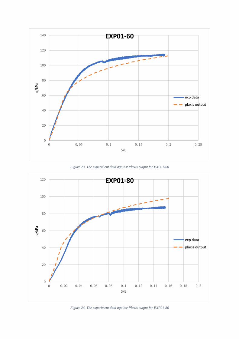
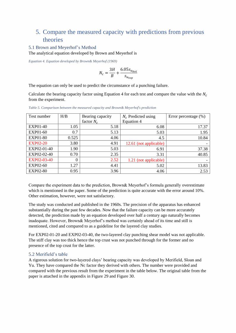
Figure 23. The experiment data against Plaxis output for EXP01-60
Figure 24. The experiment data against Plaxis output for EXP01-80
0
20
40
60
80
100
120
140
0 0.05 0.1 0.15 0.2 0.25
q/k
Pa
S/B
EXP01-60
exp data
plaxis output
0
20
40
60
80
100
120
0 0.02 0.04 0.06 0.08 0.1 0.12 0.14 0.16 0.18 0.2
q/k
Pa
S/B
EXP01-80
exp data
plaxis output

It can be observed that the trend from the FE analysis generally overlaps with the experiment data for
all three tests.
Subsequently, four simulation was conducted for EXP02 and the comparison plot can be found in the
figures below.
Figure 25. The experiment data against Plaxis output for EXP02-20
Figure 26. The experiment data against Plaxis output for EXP02-01-40
-50
0
50
100
150
200
250
0 0.05 0.1 0.15 0.2 0.25 0.3 0.35
q (
kPa)
s/B
EXP02-20
exp data
Su=24/4.93 E=2250/462.5
0
20
40
60
80
100
120
140
160
180
0 0.02 0.04 0.06 0.08 0.1 0.12 0.14 0.16 0.18 0.2
q (
kPa)
s/B
EXP02-01-40
exp data
Su=24/4.93 E=2250/462.5

Figure 27. The experiment data against Plaxis output for EXP02-60
Figure 28. The experiment data against Plaxis output for EXP02-80
The best fit for EXP02 is found when 𝑠𝑢𝑡𝑜𝑝= 24𝑘𝑃𝑎 and 𝑠𝑢𝑏𝑜𝑡
= 4.93𝑘𝑃𝑎, which again confirms the
resemblance between the FE analysis and the experiment data.
Table 8 below summarizes the comparison between the obtained Su value by experiment and by
Plaxis.
0
20
40
60
80
100
120
140
0 0.02 0.04 0.06 0.08 0.1 0.12 0.14 0.16 0.18
q (
kPa)
s/B
EXP02-60
exp data
Su=24/4.93 E=2250/462.5
-20
0
20
40
60
80
100
120
-0.02 0 0.02 0.04 0.06 0.08 0.1 0.12 0.14
q (
kPa)
s/B
80mm Footing
exp data
Su=24/4.93 E=2250/463.5

Table 8. The two sets of Su value obtained by experiment and Plaxis
Thickness for
stiff soil (mm) 𝑠𝑢 from experiment (kPa) 𝑠𝑢,𝑡𝑜𝑝
𝑠𝑢,𝑏𝑜𝑡 ratio 𝑠𝑢 from Plaxis (kPa)
𝑠𝑢,𝑡𝑜𝑝 𝑠𝑢,𝑏𝑜𝑡 𝑠𝑢,𝑡𝑜𝑝 𝑠𝑢,𝑏𝑜𝑡
EXP01 74 15.3 7.4 2.07 21 10.2
EXP02 108 20 4 5 24 4.93
Therefore, a conclusion can be drawn here based on the figures is that given the appropriate, the result
from the FE analysis can be used as a reliable method of predicting bearing capacity.

7. Conclusion The conducted experiments are proved to be successful and reasonably accurate to be used to draw
conclusions. Therefore, the separate soil consolidation and soil transfer afterwards turns out to be an
effective mean of creating two layers of soil. Hence, this method can be generalized for multiple
layered clay without having to apply the centrifuge. This provides a reliable and extremely
inexpensive way to create layered clay compare to using centrifuge, which can cost an enormous
amount of money. Besides conclusion reached relating to the research expenditure, several other facts
can be concluded in the aspect of numerical results:
1. The obtained soil stress-stain curve conforms with the soil linear-elastic plastic model.
Having the same soil properties, original gradient for all H/B value is the same at the initial
part. However, the lower the H/B value is, the sooner the gradient decreases, and ends at a
value decided by the composition of the two undrained shear strength value.
2. At low value of H/B, 𝐸0.02
𝑠𝑢 increases with the increment of H/B until it reaches a limit, with the
value around 95, after which 𝐸0.02
𝑠𝑢 remains unchanged. There is a quasi-linear relationship
between 𝐸0.02
𝑠𝑢 versus H/B but the linear relationship needs to be further investigated.
3. At low value of H/B, the bearing capacity factor Nc increases with H/B until it reaches the
limit of 5.14, after which the Nc value stays the same. The larger 𝑠𝑢𝑡𝑜𝑝
𝑠𝑢𝑏𝑜𝑡
is, the higher H/B
value need to be for Nc to reach the 5.14.
4. The soil is assumed to go through punching failure at the top crust with the bearing capacity
at the bottom failure fully developed. When H/B>2, the soil bearing capacity cannot be
estimated with any predictions derived previously.
5. For the tests that actually complies with H/B<2, after comparing the obtained bearing
capacity Nc with the previous published results, Chen’s prediction approximates the
experiment the best, Merifield’s result is moderately close. Brown and Meyerhof’s method
shows a general overestimation across the board whereas Meyerhof and Hannah’s method
grossly underestimates the Nc factor.
6. The trend of Nc in this experiment is generally in agreement with other studies.
7. The resemblance between the experiment data and the Plaxis output indicates that finite
element analysis is capable of conducting an accurate prediction, provided the correct
undrained shear strength for each soil layer is obtained.

Reference Bienen, B., 2018, “Offshore Geomechanics-shallow foundations”, Lecture notes, 72, The university
of Western Australia.
Bowles, J.E., 1979. Physical and geotechnical properties of soils.
Brown, J.D. and Meyerhof, G.G., 1969. Experimental study of bearing capacity in layered clays.
In Soil Mech & Fdn Eng Conf Proc/Mexico/.
Button, S.J., 1953. The bearing capacity of footings on a two-layer cohesive subsoil. In Proc. 3rd Int.
Conf. Soil Mech. Found. Engng, Zurich (Vol. 1, pp. 332-335).
Cai, M. ed., 2011. Rock mechanics: achievements and ambitions. CRC Press.
Chen, WF., 1975. Limit analysis and soil plasticity. Til Elsevier Scientific Publishing Company. New
York.
Davis, E.H. and Booker, J.R., 1985. The effect of increasing strength with depth on the bearing
capacity of clays. Golden Jubilee of the International Society for Soil Mechanics and Foundation
Engineering: Commemorative Volume, p.185.
Goss, C.M. and Griffiths, D.V., 2001. Rigorous plasticity solutions for the bearing capacity of two-
layered clays. Geotechnique, 51(2), pp.179-183.
Lehane, B.M., 2017. “Applied Geomechanics.” Course reader, 49,94, The university of Western
Australia.
Merifield, R.S. and Nguyen, V.Q., 2006. Two-and three-dimensional bearing-capacity solutions for
footings on two-layered clays. Geomechanics and Geoengineering: An International Journal, 1(2),
pp.151-162.
Merifield, R.S., Sloan, S.W. and Yu, H.S., 1999. Rigorous plasticity solutions for the bearing capacity
of two-layered clays. Geotechnique, 49(4), pp.471-490.
Meyerhof, G.G. and Hanna, A.M., 1978. Ultimate bearing capacity of foundations on layered soils
under inclined load. Canadian Geotechnical Journal, 15(4), pp.565-572.
Reddy, A.S. and Srinivasan, R.J., 1967. Bearing capacity of footings on layered clays. Journal of the
Soil Mechanics and Foundations Division, 93(2), pp.83-99.
Sloan, S.W., 1988. Lower bound limit analysis using finite elements and linear
programming. International Journal for Numerical and Analytical Methods in Geomechanics, 12(1),
pp.61-77.
Sloan, S.W. and Kleeman, P.W., 1995. Upper bound limit analysis using discontinuous velocity
fields. Computer methods in applied mechanics and engineering, 127(1-4), pp.293-314.
Terzaghi, K., 1943, Theoretical Soil Mechanics, John Wiley & Sons, New York.
Wang, C.X. and Carter, J.P., 2002. Deep penetration of strip and circular footings into layered
clays. International Journal of Geomechanics, 2(2), pp.205-232.
Wegener, A., 1966. The origin of continents and oceans. Courier Corporation.
Yu, L., Liu, J., Kong, X.J. and Hu, Y., 2010. Three-dimensional large deformation FE analysis of
square footings in two-layered clays. Journal of geotechnical and geoenvironmental
engineering, 137(1), pp.52-58.

Zhu, M. and Michalowski, R.L., 2005, September. Bearing capacity of rectangular footings on two-
layer clay. In Proceedings of the International Conference on Soil Mechanics and Geotechnical
Engineering (Vol. 16, No. 2, p. 997). AA BALKEMA PUBLISHERS.

Appendix
Figure 29. The bearing capacity factor Nc for Meyerhof (row 345), Chen and Meyerhof& Hanna's solution

Figure 30. The bearing capacity factor Nc for Meyerhof (row 345), Chen and Meyerhof& Hanna's solution (cont)