Stiffness Estimation and Nonlinear Control of Robots with

Stiffness Estimation and Nonlinear Controlof Robots with Variable Stiffness Actuation

Fabrizio Flacco Alessandro De Luca

Dipartimento di Informatica e SistemisticaUniversita di Roma “La Sapienza”, Via Ariosto 25, 00185 Roma, Italy

{fflacco,deluca}@dis.uniroma1.it

Abstract: We consider the problem of estimating on line the nonlinear stiffness of flexibletransmissions in robots with variable stiffness actuation in agonistic-antagonistic configuration.Stiffness estimation is obtained using a dynamic residual that provides a filtered version ofthe unmeasured flexibility torques, combining it with a recursive least squares algorithm thatfits a polynomial model to the data, and proceeding then by analytical derivation. Onlymotor position/velocity and link position measurements are used, while knowledge of dynamicparameters is required for the motors but not for the links. The estimated stiffness function,together with its first two derivatives with respect to the deformation, is used within a feedbacklinearization controller designed for simultaneous tracking of desired trajectories for the linksand the device stiffnesses. Simulation results provided for the VSA-II device demonstrate theperfomance of the estimation process and the effectiveness of the complete control approach.

Keywords: Flexible transmissions, Variable stiffness actuation, Stiffness estimation, Recursiveleast squares, Feedback linearization control, Robot motion control

1. INTRODUCTION

For a safer physical Human-Robot Interaction (pHRI),compliant elements are introduced in robot manipulatorsat different levels in the structure, including end-effectortools, link surfaces, and robot joints, transmissions, andactuation devices (De Santis et al. (2008)). A compliant(non-stiff) robot allows to milden the danger of injuries tothe human user due to accidental collisions. In particular,the use of flexible transmissions reduces the effective in-ertia seen during a dynamic impact with the environmentthanks to the mechanical decoupling between the relativelylarge motor inertias and the inertia of the (lightweight)robot links. On the other hand, flexible transmissionswill challenge the control performance in preventing vi-brations, accurately tracking reference trajectories, andlimiting energy consumption (De Luca and Book (2008)).

One recent trend in pHRI is to design robots using variablestiffness actuation (VSA) devices, see Bicchi and Tonietti(2004); Tonietti et al. (2005); Wolf and Hirzinger (2008);Catalano et al. (2010). In this context, the mechanicalstiffness of a robot joint is defined as the relation betweenthe displacement at the link side of the transmission andthe flexibility torque that arises in reaction. The jointsof an industrial robot equipped with harmonic drivesdisplay a constant stiffness, i.e., the transmissions canbe modeled by springs that work in their linear elasticdomain. In contrast, in order to obtain a (passive or active)variation of joint stiffness during robot motion, the flexibletransmission should behave in a nonlinear way. This canbe obtained either through a spring with nonlinear (e.g.,cubic or exponential) deformation-torque characteristic orwith an elastic spring of constant stiffness mounted in a

nonlinear kinematic arrangement. In VSA-based robots,two independent motors are used at each joint and motionis transmitted through nonlinear flexible transmissionsassembled in various configurations. One example, whichwill be used in this paper, is given by the VSA-II devicedeveloped at the University of Pisa by Schiavi et al. (2008),where the two actuators work in a parallel, agonistic-antagonistic, bi-directional, and (nominally) symmetricmode. With two actuators, it is possible to actively controlthe motion of the links/load while modifying on line(from softer to harder and viceversa) the stiffness of thejoints. A safe and energy efficient behavior is obtained,e.g., by imposing a small stiffness at high link velocitiesand a large stiffness at low velocities, as in the safebrachistochrone planning solution introduced by Bicchiand Tonietti (2004).

Feedback control laws intended for regulation and/or tra-jectory tracking in robots with flexible joints typically needa good knowledge of the robot dynamic parameters, in-cluding joint stiffness, see, e.g., De Luca and Book (2008);Tonietti et al. (2005). Under the ideal assumptions that aperfect model is available and that the full robot state ismeasured, De Luca et al. (2009) have shown that a singlelink moving under gravity and driven by a VSA antagonis-tic device can be exactly linearized by means of nonlinearfeedback. This result can be easily extended to the gen-eral multi-link case. The proposed feedback linearizationdesign enables simultaneous and decoupled control of linkmotion and joint stiffness, achieving exponentially stabletracking of sufficiently smooth reference profiles for thesequantities.

Unfortunately, there are no available sensors for a directmeasure of stiffness. This physical quantity is usually

Proceedings of the 18th World CongressThe International Federation of Automatic ControlMilano (Italy) August 28 - September 2, 2011

978-3-902661-93-7/11/$20.00 © 2011 IFAC 6872 10.3182/20110828-6-IT-1002.03299

computed from position and/or joint torque sensor data,based on a nominal model and static calibration. Thisprocedure is especially critical in VSA-based robots, sincethe stiffness is intrinsically a nonlinear function of thejoint deformation, its model may have a quite complex(and uncertain) expression, and the rigid body dynamicsof the driven robot links is highly nonlinear. In addition,since the device stiffness that should be controlled is notdirectly measured, an intrinsic robustness limitation arises:at best, the nominal or estimated stiffness output (and notthe actual one) can track the desired reference.

The above considerations motivated the need for on-line methods of stiffness estimation in VSA-based robots.While some authors have dealt with stiffness estimation inthe contact between the end-effector of a rigid robot andthe environment/human (see, e.g., Diolaiti et al. (2005);Verscheure et al. (2009); Ludvig and Kearney (2009);Coutinho and Cortesao (2010)), work on estimation ofvariable, nonlinear stiffness of single- or double-actuatedflexible joints is still at the beginning. Grioli and Bicchi(2010) have introduced a stiffness estimator based on theknowledge of the flexibility torque, which is in turn explic-itly measured by a sensor. Their estimator processes thetime derivative of the measured flexibility torque, whichmay give problems due to noise. A batch (almost on-line)estimation method that does not use joint torque sensingnor acceleration estimation has been recently proposedby Flacco and De Luca (2011).

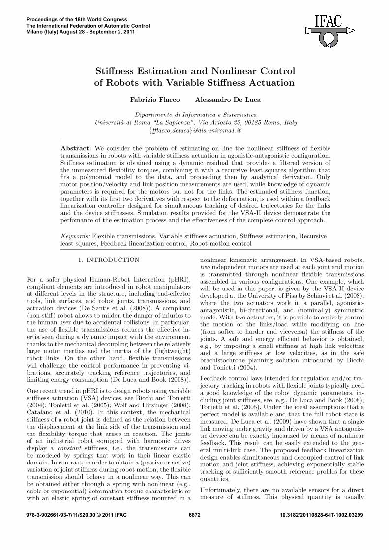
In this paper, we present a new method for on-line stiffnessestimation for VSA-based robots and its use within a feed-back linearization control scheme. The developments aremade for a single-dof agonistic-antagonistic system undergravity, but can be easily extended to multi-dof robots.For stiffness estimation, we will only use the knowledgeof dynamic parameters (inertia and viscous friction coeffi-cient) of the two motors and measures of the motor posi-tion and velocity and of the link position. Our estimationapproach uses two basic tools: i) a residual-based method,as inherited from FDI techniques (see, e.g., De Luca andMattone (2003); Haddadin et al. (2008)), which providesa filtered version of the (unmeasured) flexibility torquesat the joint, and ii) a standard Recursive Least Squares(RLS) algorithm that fits the residual data to a generalparametrized model, which is chosen as a polynomial inthe transmission deformation. From this estimated model,we can compute analytically the stiffness and its firsttwo derivatives with respect to the joint deformation, asneeded by the feedback linearization controller of De Lucaet al. (2009). Based on the certainty equivalence principle,the resulting on-line estimates are fed into the nonlinearcontroller. The proposed estimation/control approach issummarized in the scheme of Fig. 1.

The paper is organized as follows. In Sect. 2 we present thedynamic modeling framework. The residual design for on-line estimation of the flexibility torque is given in Sect. 3.The model-based estimation of transmission stiffness usinga RLS algorithm is discussed in Sect. 4, together withan error recovery scheme to compensate for the filteringaction of the residual (Sect. 4.1). In Sect. 5, numericalresults on stiffness estimation are reported for the VSA-IIdevice moving a link under gravity. Finally, Section 6revisits the feedback linearization control law introduced

VSAII

FBL

control

Motor torques

Residual

generator

Motorposition andvelocity

RLS

+

RER

Linkposition

Estimates offlexibility transmission

components

Linear

control

[v1, v2]Link positionand stiffnessreferences

+

Estimatedstiffness

-

Fig. 1. Scheme of stiffness estimation and its use infeedback linearization control

by De Luca et al. (2009) when on-line estimates of allquantities related to stiffness are used, and illustrates theobtained closed-loop performance by simulations.

2. DYNAMIC MODELING

Consider a flexible transmission that connects a drivingmotor to the driven link. The deformation φ = q − θ ofthe transmission is the difference between the motor angleθ and the link angle q. A potential function Ue(φ) ≥ 0is associated to the deformation φ, with Ue(φ) = 0 iffφ = 0. The flexibility torque across the transmission isτe(φ) = ∂Ue(φ)/∂φ, and based on physical arguments andcurrent implementations it can be assumed that

τe(0) = 0, τe(−φ) = −τe(φ), ∀φ. (1)The stiffness of the transmission is defined as the variationof the flexibility torque w.r.t. link displacements

σ(φ) =∂τe(φ)∂q

=∂τe(φ)∂φ

> 0. (2)

For a single motor driving a rigid link subject to gravitythrough a (nonlinear) flexible transmission, the dynamicmodel takes the form

Mq +Dq q + τe(φ) + g(q) = 0 (3)

Bθ +Dθ θ − τe(φ) = τ, (4)where M > 0 and B > 0 are the link and motor inertias,Dq ≥ 0 and Dθ ≥ 0 are the viscous friction coefficients atthe two sides of the transmission, τ is the torque providedby the motor (after gear reduction), and g(q) is the gravitytorque acting on the link.

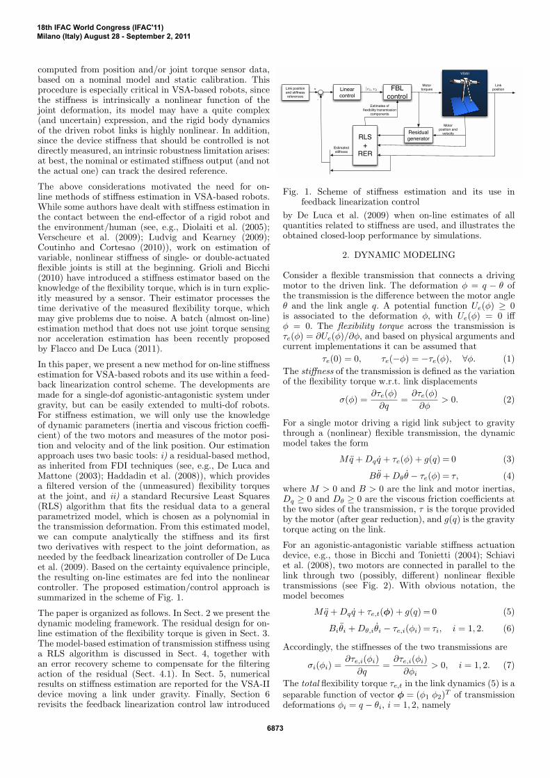
For an agonistic-antagonistic variable stiffness actuationdevice, e.g., those in Bicchi and Tonietti (2004); Schiaviet al. (2008), two motors are connected in parallel to thelink through two (possibly, different) nonlinear flexibletransmissions (see Fig. 2). With obvious notation, themodel becomes

Mq +Dq q + τe,t(φ) + g(q) = 0 (5)

Biθi +Dθ,iθi − τe,i(φi) = τi, i = 1, 2. (6)

Accordingly, the stiffnesses of the two transmissions are

σi(φi) =∂τe,i(φi)

∂q=∂τe,i(φi)∂φi

> 0, i = 1, 2. (7)

The total flexibility torque τe,t in the link dynamics (5) is aseparable function of vector φ = (φ1 φ2)T of transmissiondeformations φi = q − θi, i = 1, 2, namely

18th IFAC World Congress (IFAC'11)Milano (Italy) August 28 - September 2, 2011

6873

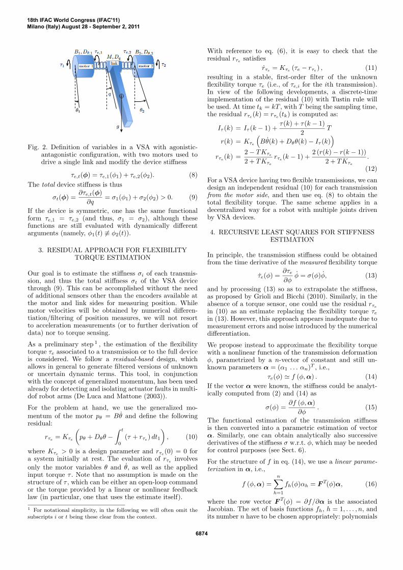
Fig. 2. Definition of variables in a VSA with agonistic-antagonistic configuration, with two motors used todrive a single link and modify the device stiffness

τe,t(φ) = τe,1(φ1) + τe,2(φ2). (8)The total device stiffness is thus

σt(φ) =∂τe,t(φ)∂q

= σ1(φ1) + σ2(φ2) > 0. (9)

If the device is symmetric, one has the same functionalform τe,1 = τe,2 (and thus, σ1 = σ2), although thesefunctions are still evaluated with dynamically differentarguments (namely, φ1(t) 6≡ φ2(t)).

3. RESIDUAL APPROACH FOR FLEXIBILITYTORQUE ESTIMATION

Our goal is to estimate the stiffness σi of each transmis-sion, and thus the total stiffness σt of the VSA devicethrough (9). This can be accomplished without the needof additional sensors other than the encoders available atthe motor and link sides for measuring position. Whilemotor velocities will be obtained by numerical differen-tiation/filtering of position measures, we will not resortto acceleration measurements (or to further derivation ofdata) nor to torque sensing.

As a preliminary step 1 , the estimation of the flexibilitytorque τe associated to a transmission or to the full deviceis considered. We follow a residual-based design, whichallows in general to generate filtered versions of unknownor uncertain dynamic terms. This tool, in conjunctionwith the concept of generalized momentum, has been usedalready for detecting and isolating actuator faults in multi-dof robot arms (De Luca and Mattone (2003)).

For the problem at hand, we use the generalized mo-mentum of the motor pθ = Bθ and define the followingresidual:

rτe= Kτe

(pθ +Dθθ −

∫ t

0

(τ + rτe) dt1

), (10)

where Kτe> 0 is a design parameter and rτe

(0) = 0 fora system initially at rest. The evaluation of rτe

involvesonly the motor variables θ and θ, as well as the appliedinput torque τ . Note that no assumption is made on thestructure of τ , which can be either an open-loop commandor the torque provided by a linear or nonlinear feedbacklaw (in particular, one that uses the estimate itself).

1 For notational simplicity, in the following we will often omit thesubscripts i or t being these clear from the context.

With reference to eq. (6), it is easy to check that theresidual rτe

satisfiesrτe

= Kτe(τe − rτe

) , (11)resulting in a stable, first-order filter of the unknownflexibility torque τe (i.e., of τe,i for the ith transmission).In view of the following developments, a discrete-timeimplementation of the residual (10) with Tustin rule willbe used. At time tk = kT , with T being the sampling time,the residual rτe

(k) = rτe(tk) is computed as:

Iτ (k) = Iτ (k − 1) +τ(k) + τ(k − 1)

2T

r(k) = Kτe

(Bθ(k) +Dθθ(k)− Iτ (k)

)rτe(k) =

2− TKτe

2 + TKτe

rτe(k − 1) +2 (r(k)− r(k − 1))

2 + TKτe

.

(12)

For a VSA device having two flexible transmissions, we candesign an independent residual (10) for each transmissionfrom the motor side, and then use eq. (8) to obtain thetotal flexibility torque. The same scheme applies in adecentralized way for a robot with multiple joints drivenby VSA devices.

4. RECURSIVE LEAST SQUARES FOR STIFFNESSESTIMATION

In principle, the transmission stiffness could be obtainedfrom the time derivative of the measured flexibility torque

τe(φ) =∂τe∂φ

φ = σ(φ)φ, (13)

and by processing (13) so as to extrapolate the stiffness,as proposed by Grioli and Bicchi (2010). Similarly, in theabsence of a torque sensor, one could use the residual rτe

in (10) as an estimate replacing the flexibility torque τein (13). However, this approach appears inadequate due tomeasurement errors and noise introduced by the numericaldifferentiation.

We propose instead to approximate the flexibility torquewith a nonlinear function of the transmission deformationφ, parametrized by a n-vector of constant and still un-known parameters α = (α1 . . . αn)T , i.e.,

τe(φ) ' f (φ,α) . (14)If the vector α were known, the stiffness could be analyt-ically computed from (2) and (14) as

σ(φ) =∂f (φ,α)

∂φ. (15)

The functional estimation of the transmission stiffnessis then converted into a parametric estimation of vectorα. Similarly, one can obtain analytically also successivederivatives of the stiffness σ w.r.t. φ, which may be neededfor control purposes (see Sect. 6).

For the structure of f in eq. (14), we use a linear parame-terization in α, i.e.,

f (φ,α) =n∑h=1

fh(φ)αh = F T(φ)α, (16)

where the row vector F T(φ) = ∂f/∂α is the associatedJacobian. The set of basis functions fh, h = 1, . . . , n, andits number n have to be chosen appropriately: polynomials


6874

of increasing order are a general and convenient choice. Inparticular, taking into account the physical property (1) ofthe flexibility torque, we select only the first n odd powersof φ up to the order 2n− 1:

fh(φ) = φ2h−1, h = 1, . . . , n. (17)

To obtain an estimate α of the parameter vector α, weadopt a least squares method in discrete time. At timetk = kT , the deformation φ(k) = φ(tk) and the resid-ual rτe

(k) = rτe(tk) are collected as data points. The

parameters estimate α is chosen so as to minimize thecost function E given by the sum of the squared differ-ences between the observed residuals and the estimatedtransmission flexibility torque, i.e.,

E =12

p∑k=1

(rτe(k)− f (φ(k), α)

)2, (18)

where p > n is a sufficient number of collected data points.The solution of the estimation problem in batch form is

α =

(p∑k=1

F (k)F T(k)

)−1( p∑k=1

F (k) rτe(k)

), (19)

where the Jacobian F T(k) is

F T(k) =(φ(k) φ3(k) . . . φ2n−1(k)

). (20)

Since on-line parameter estimation is more suitable forcontrol purposes, the estimate (19) should be updatedrecursively at each sampling time. The standard RecursiveLeast Squares (RLS) algorithm is

α(k) = α(k − 1) + ∆α(k), (21)with

∆α(k) = L(k)(rτe(k)− F T(k)α(k − 1)

)(22)

where

L(k) =P (k − 1)F (k)

1 + F T(k)P (k − 1)F (k)(23)

andP (k) =

(I −L(k)F T(k)

)P (k − 1), (24)

being P (k) the n×n covariance matrix and I the identitymatrix. As opposed to (19), the recursive algorithm suffersless from possible ill-conditioning of F . The algorithm isinitialized with an a priori estimate α(0) and a positivedefinite (usually, diagonal) choice P (0) for the covariancematrix. This matrix is typically initialized with largevalues, considering no a priori knowledge about the trueparameter vector α. For a convergence analysis of the RLSalgorithm, see, e.g., Johnson (1988).

The degree n of the polynomial f (φ(k),α) in (16) shouldbe large enough to capture the nonlinearities of the trans-mission flexibility torque, especially if large deformationsoccur. Otherwise, even when the estimate converges andthe covariance matrix P becomes small, the RLS estimatewill no longer track efficiently the residual data (see alsothe example in Sect. 5). The appropriate degree of thepolynomial approximation can be tested using a numberof indicators, the simplest of which is E itself in (18).

Summarizing, for any parametrized model (16) used toapproximate the flexibility torque, the current estimateα(k) obtained with the RLS algorithm provides a stiffnessestimate given by

σ(k) =∂f (φ, α(k))

∂φ=

n∑h=1

∂fh(φ)∂φ

αh(k). (25)

Indeed, this stiffness estimation procedure can be applied(simultaneously) to both transmissions of the VSA system,yielding σ1(k) and σ2(k) and thus σt(k) = σ1(k) + σ2(k)for the total device stiffness, according to (9).

4.1 Residual Error Recovery (RER)

A simple improvement of the residual-based RLS estima-tion of the flexibility torque, and thus of the transmissionstiffness, can be obtained as follows. From eq. (11), theresidual error can be expressed as

εr = τe(φ)− rτe=

rτe

Kτe

. (26)

Therefore, a first possibility is to approximate the residualerror εr with backward differences in discrete time, namelyusing

εr(k) =rτe

(k)− rτe(k − 1)

TKτe

. (27)

A second possibility is based on the approximate relationrτe ≈ τe(φ). (28)

Using (13), with the current estimate σ(k) given by (25)and a measure of φ(k) = q(k) − θ(k), an estimate of theresidual error εr in (26) is provided at each step k by

εr(k) =σ(k)φ(k)Kτe

. (29)

The choice between (27) and (29) depends on the kind ofsensors used and on the measurement noise. In any event,we can use εr(k) to compensate for the time lag introducedby the residual, replacing (22) with

∆α(k) = L(k)(rτe

(k) + εr(k)− F T (k)α(k − 1)). (30)

5. ESTIMATION RESULTS

We illustrate the performance of the proposed residual-based RLS estimation of stiffness on the VSA-II devicedeveloped by Schiavi et al. (2008). In this antagonisticVSA device, the nonlinear characteristics of each of thetwo flexible transmissions is obtained thanks to a pair of4-bar linkages with linear springs. The flexibility torque ofeach transmission can be modeled as

τe,i(φi) = 2 ki β(φi)∂β(φi)∂φi

, i = 1, 2, (31)

where ki > 0 is the constant stiffness of the spring in thei-th transmission, and

β(φi) = arcsin(Ci sin

(φi2

))− φi

2, i = 1, 2, (32)

being Ci > 1 a geometric non-dimensional parameter ofthe linkage. The total flexibility torque τe,t acting on thelink dynamics (5) is given by eq. (8). Note that in themodel of τe,i the two uncertain parameters ki and Ciappear, respectively, in a linear and nonlinear way.

The nominal dynamic parameters for the simulations ofthis robotic system are those reported by Schiavi et al.(2008). In particular, the four parameters that charac-terize the flexible transmissions are Ci = 1.75 and ki =


6875

0 1 2 3 4 5 6 7 8 9 10−0.8

−0.6

−0.4

−0.2

0

0.2

0.4

0.6

Time (s)

Tra

nsm

issio

n D

efo

rma

tio

n (

rad

)

Φ1

Φ2

Fig. 3. Transmission deformations φ1, φ2 for the VSA-IIdevice under the sinusoidal torque inputs (33)

0 1 2 3 4 5 6 7 8 9 10−120

−100

−80

−60

−40

−20

0

20

Time (s)

Fle

xib

ility

To

rqu

e (

Nm

m)

Estimated

Actual

(a)

0 1 2 3 4 5 6 7 8 9 10−150

−100

−50

0

50

100

150

Time (s)

Fle

xib

ility

To

rqu

e (

Nm

m)

Estimated

Actual

(b)

Fig. 4. Comparison of residual rτe in (12) and nominalflexibility torque τe for the first (a) and second (b)transmission

500 [N·mm/rad], for i = 1, 2. Applying for 10 sec the open-loop torquesτ1 = 10 · sin 0.1π τ2 = 10 · sin 0.2π [N·mm], (33)

starting from an undeformed equilibrium configurationwith the link pointing downward (under gravity), weobtained the transmission deformations φ1 and φ2 shownin Fig. 3. Figure 4 compares the associated residualscomputed by (12), using Kτe = 300 and a sampling timeT = 0.1 msec, with the evolution of the nominal flexibilitytorques of the two transmissions. No differences can beappreciated in practice.

For stiffness estimation, the residual-based RLS algo-rithm (21–24) has been applied with n = 4 polynomialterms in (16–17), an initial parameter estimate α(0) = 0and an initial 4 × 4 covariance matrix P (0) = 106I. Foreach of the two VSA-II transmissions, Figures 5 and 6 showthe time evolution of the estimated stiffness in comparisonwith the nominal one and a few snapshots (at t = 0.5, 1,and 10 sec) of how the approximating function progressestoward the nominal stiffness characteristic. Convergenceto the actual current value of stiffness occurs within onethird of the total motion time. On the other hand, the

0 1 2 3 4 5 6 7 8 9 100

50

100

150

200

250

300

350

Time (s)

Stiff

ne

ss (

Nm

m/r

ad

)

Estimated

Actual

(a)

−1 −0.8 −0.6 −0.4 −0.2 0 0.2 0.4 0.6 0.8 1−2500

−2000

−1500

−1000

−500

0

500

1000

1500

2000

2500

Transmission Deformation (rad)

Stiff

ne

ss (

Nm

m/r

ad

)

Estimated 0.5 sec

Estimated 1 sec

Estimated 10 sec

Actual

(b)

Fig. 5. Comparison of estimated and nominal stiffness (a)and the approximating stiffness function at selectedinstants (b) for the first transmission of the VSA-II

0 1 2 3 4 5 6 7 8 9 100

50

100

150

200

250

300

350

Time (s)

Stiff

ne

ss (

Nm

m/r

ad

)

Estimated

Actual

(a)

−1 −0.8 −0.6 −0.4 −0.2 0 0.2 0.4 0.6 0.8 10

1000

2000

3000

4000

5000

6000


Stiff

ne

ss (

Nm

m/r

ad

)

Estimated 0.5 sec

Estimated 1 sec

Estimated 10 sec

Actual

(b)

Fig. 6. Same plots as in Fig. 5 for the second transmission

curve fitting of the complete characteristics is poor fordeformations that are larger in module than 0.6 rad. Thisshould not be unexpected since such large deformations(see Fig. 3) do not occur during the specific motion ob-tained under the torque commands (33).

Next, we have evaluated the effects of the residual errorrecovery scheme of Sect. 4.1 in the RLS stiffness estimator.Figures 7 and 8 show the benefit obtained when using (30).The time needed to converge to the the nominal stiffnessis largely reduced, while spurious transient phenomena


6876

0 1 2 3 4 5 6 7 8 9 100

50

100

150

200

250

300

350

Time (s)

Stiff

ne

ss (

Nm

m/r

ad

)

Estimated

Actual

(a)

−1 −0.8 −0.6 −0.4 −0.2 0 0.2 0.4 0.6 0.8 10

500

1000

1500

2000

2500


Stiff

ne

ss (

Nm

m/r

ad

)

Estimated 0.5 sec

Estimated 1 sec

Estimated 10 sec

Actual

(b)

Fig. 7. Comparison of estimated and nominal stiffness (a)and the approximating stiffness function at selectedinstants (b) for the first transmission of the VSA-II,when using the residual error recovery

0 1 2 3 4 5 6 7 8 9 100

50

100

150

200

250

300

350

Time (s)

Stiff

ne

ss (

Nm

m/r

ad

)

Estimated

Actual

(a)

−1 −0.8 −0.6 −0.4 −0.2 0 0.2 0.4 0.6 0.8 10

500

1000

1500

2000

2500


Stiff

ne

ss (

Nm

m/r

ad

)

Estimated 0.5 sec

Estimated 1 sec

Estimated 10 sec

Actual

(b)

Fig. 8. Same plots as in Fig. 7 for the second transmission

on the approximating function are eliminated —compare,e.g., the situation at t = 1 sec in Figs. 5(b) and 7(b).

Finally, to illustrate the problems of an under-parametrizedmodel, we report in Fig. 9 the results on stiffness estima-tion when the number of terms in the polynomial (16–17)approximating the flexibility torque is reduced to n = 2.A permanent and recurrent error is clearly left.

0 1 2 3 4 5 6 7 8 9 100

50

100

150

200

250

300

350

Time (s)

Stiff

ne

ss (

Nm

m/r

ad

)

Estimated

Actual

(a)

0 1 2 3 4 5 6 7 8 9 100

50

100

150

200

250

300

350

Time (s)

Stiff

ne

ss (

Nm

m/r

ad

)

Estimated

Actual

(b)

Fig. 9. Stiffness estimation for the VSA-II device whenusing n = 2 terms in the polynomial approximation(16–17); first (a) and second (b) transmission

6. FEEDBACK LINEARIZATION CONTROL

In this section, we combine the proposed on-line stiffnessestimator with the feedback linearization (FBL) controllerfor the VSA-II robotic system introduced by De Lucaet al. (2009). For the details on the feedback linearizationdesign, the reader is referred to the original publication.The linearizing coordinates for system (5–6) are the linkposition q together with its first three time derivatives,and the device stiffness σt with its first derivative. Thestate x = (q, q, θ1, θ1, θ2, θ2) is thus diffeomorphic to thetransformed state z = (q, q, q, q[3], σt, σt). Therefore, thedynamics of the VSA-II system can be rewritten as(

q[4]

σt

)= A(x)

(τ1τ2

)+ b(x), (34)

where A(x) is the so called decoupling matrix

A(x) = Γ

σ1 σ2

∂σ1

∂φ1

∂σ2

∂φ2

, (35)

being Γ a constant, diagonal, and invertible matrix, andb(x) a computable function of x. The complete expressionsof Γ and b(x) are given in Appendix A. It can be shownthat the decoupling matrix is always invertible providedthat φ1 6= φ2, a condition that can be safely avoided by asuitable pre-charging of the system.

The dynamic equations (34) can be exactly linearized(and input-output decoupled) using the nonlinear statefeedback law(

τ1τ2

)= A−1(x)

((v1v2

)− b(x)

), (36)

where v1 and v2 are the new control inputs. These canbe designed for stable trajectory tracking purposes onthe linear and decoupled side of the problem. In fact,the closed-loop system given by (34) and (36) is made


6877

by two independent chains of input-output integrators(four integrators between v1 and the link position q andtwo between v2 and the device stiffness σt). The trackingerrors with respect to smooth reference trajectories qd(t)for the link position and σt,d(t) for the device stiffness isexponentially stabilized by a PD3 error feedback law forv1 (with suitable positive gains characterizing a Hurwitzpolynomial) and a PD error feedback law for v2 (withpositive gains), plus the feedforward terms, respectivelyq[4]d (t) and σt,d(t).

Assume now that all dynamic parameters in eqs. (5–6) areknown, except for those related to the transmission flexi-bility. The unknown components required for implement-ing the feedback linearization law (36) are the flexibilitytorques τe1 and τe2 and the transmission stiffnesses σ1 andσ2, together with their first and second derivatives w.r.t.the deformations φ1 and φ2. More explicitly, we need ∂σ1

∂φ1,

∂σ2∂φ2

, ∂2σ1∂φ2

1, and ∂2σ2

∂φ22

. The last two quantities are used inthe evaluation of b(x), see again Appendix A.

Using the proposed estimator, for each transmission of theVSA-II we can evaluate (dropping the index i = 1, 2)

τe(φ) = f (φ, α) =n∑h=1

φ2h−1 αh (37)

σ(φ) =n∑h=1

(2h− 1)φ2h−2 αh (38)

∂σ(φ)∂φ

=n∑h=2

(4h2 − 6h+ 2)φ2h−3 αh (39)

∂2σ(φ)∂φ2

=n∑h=2

(8h3 − 24h2 + 22h− 6)φ2h−4 αh, (40)

and insert these in place of the unknown terms. Theintegration of the proposed estimator within the FBLcontroller leads to the scheme shown in Fig. 1.

0 0.5 1 1.5 2 2.5 3 3.5 4 4.5 50

0.2

0.4

0.6

0.8

1

1.2

1.4

1.6

Time (s)

Lin

k p

ositio

n (

rad

)

Actual

Desired

(a)

0 0.5 1 1.5 2 2.5 3 3.5 4 4.5 5−0.005

0

0.005

0.01

0.015

0.02

0.025

0.03

0.035

Time (s)

Lin

k p

ositio

n e

rror

(rad)

(b)

Fig. 10. Reference and actual link position with FBL con-trol using stiffness estimation (a) and link trajectorytracking error (b)

0 0.5 1 1.5 2 2.5 3 3.5 4 4.5 50

200

400

600

800

1000

1200

1400

1600

1800

2000

Time (s)

Stiff

ne

ss (

Nm

m/r

ad

)

Actual

Estimated

Reference

(a)

0 0.5 1 1.5 2 2.5 3 3.5 4 4.5 5

−0.1

−0.05

0

0.05

0.1

0.15

Time (s)

Stiffness c

ontr

ol err

or

(Nm

m/r

ad)

(b)

0 0.5 1 1.5 2 2.5 3 3.5 4 4.5 5−20

−10

0

10

20

30

40

Time (s)

Stiffness e

stim

ation e

rror

(Nm

m/r

ad)

(c)

Fig. 11. Reference, estimated, and actual stiffness trajec-tory obtained with FBL control using stiffness estima-tion (a), reference−estimated stiffness control error(b), and stiffness estimation error (c)

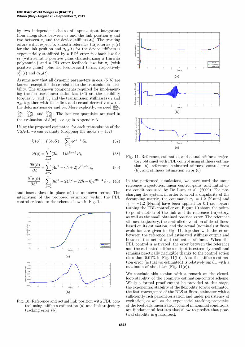
In the performed simulations, we have used the samereference trajectories, linear control gains, and initial er-ror conditions used by De Luca et al. (2009). For pre-charging the system, in order to avoid a singularity of thedecoupling matrix, the commands τ1 = 1.2 [N·mm] andτ2 = −1.2 [N·mm] have been applied for 0.1 sec, beforeturning the FBL controller on. Figure 10 shows the point-to-point motion of the link and its reference trajectory,as well as the small obtained position error. The referencestiffness trajectory, the controlled evolution of the stiffnessbased on its estimation, and the actual (nominal) stiffnessevolution are given in Fig. 11, together with the errorsbetween the reference and estimated stiffness output andbetween the actual and estimated stiffness. When theFBL control is activated, the error between the referenceand the estimated stiffness output is extremely small andremains practically negligible thanks to the control action(less than 0.01% in Fig. 11(b)). Also the stiffness estima-tion error (actual vs. estimated) is relatively small, with amaximum of about 2% (Fig. 11(c)).

We conclude this section with a remark on the closed-loop stability of the complete estimation-control scheme.While a formal proof cannot be provided at this stage,the exponential stability of the flexibility torque estimator,the fast convergence of the RLS stiffness estimator with asufficiently rich parameterization and under persistency ofexcitation, as well as the exponential tracking propertiesof the feedback linearization control in nominal conditions,are fundamental features that allow to predict that prac-tical stability is guaranteed.


6878

7. CONCLUSIONS

A novel on-line stiffness estimation method for robotswith variable stiffness actuation in agonistic-antagonisticconfiguration has been proposed, and its output has beencombined with an advanced motion/stiffness controllerbased on feedback linearization and input-output decou-pling. Since the stiffness of each transmission is estimatedindependently and locally at each motor side, the esti-mator requires no information on the link dynamics andlimited sensing, in particular no joint torque sensor. Theintegration of the stiffness estimator with the feedbacklinearizing controller has been presented for a single-linkdevice (also with non-symmetric dynamic and flexibilityproperties), but can be extended to the case of multi-linkrobots using VSA in a straightforward way.

After the satisfactory results obtained in simulations, weare planning an experimental verification on the VSA-IIsystem, in collaboration with the University of Pisa. More-over, we are currently extending the estimation approachalso to other VSA configurations, e.g., using harmonicdrives with variable stiffness (Wolf and Hirzinger (2008);Catalano et al. (2010)). In Flacco et al. (2011), we presentpreliminary experiments on the stiffness estimation for theIIT AwAS, a VSA device in serial configuration where aprimary motor controls link motion and a secondary motoris used to adjust stiffness.

REFERENCES

Bicchi, A. and Tonietti, G. (2004). Fast and soft armtactics: Dealing with the safety-performance trade-offin robot arms design and control. IEEE Robotics andAutomation Mag., 11(2), 22–33.

Catalano, M., Schiavi, R., and Bicchi, A. (2010). Designof variable stiffness actuators mechanisms based onenumeration and analysis of performance. In Proc. IEEEInt. Conf. on Robotics and Automation, 3285–3291.

Coutinho, F. and Cortesao, R. (2010). System stiffnessestimation with the candidate observers algorithm. InProc. 18th Mediterranean Conf. on Control and Au-tomation, 796–801.

De Luca, A. and Book, W. (2008). Robots with flexibleelements. In B. Siciliano and O. Khatib (eds.), SpringerHandbook of Robotics, 287–319. Springer.

De Luca, A., Flacco, F., Bicchi, A., and Schiavi, R.(2009). Nonlinear decoupled motion-stiffness controland collision detection/reaction for the VSA-II variablestiffness device. In Proc. IEEE/RSJ Int. Conf. onIntelligent Robots and Systems, 5487–5494.

De Luca, A. and Mattone, R. (2003). Actuator failuredetection and isolation using generalized momenta. InProc. IEEE Int. Conf. on Robotics and Automation,634–639.

De Santis, A., Siciliano, B., De Luca, A., and Bicchi, A.(2008). An atlas of physical human-robot interaction.Mechanism and Machine Theory, 43(3), 253–270.

Diolaiti, N., Melchiorri, C., and Stramigioli, S. (2005).Contact impedance estimation for robotic systems.IEEE Trans. on Robotics, 21(5), 925–935.

Flacco, F. and De Luca, A. (2011). Residual-based stiffnessestimation in robots with flexible transmissions. To bepresented at IEEE Int. Conf. on Robotics and Automa-tion, Shanghai, PRC (May 2011).

Flacco, F., De Luca, A., Sardellitti, I., and Tsagarakis, N.(2011). Robust estimation of variable stiffness in flexiblejoints. Submitted to IEEE/RSJ Int. Conf. on IntelligentRobots and Systems, San Francisco, CA (Sep. 2011).

Grioli, G. and Bicchi, A. (2010). A non-invasive real-time method for measuring variable stiffness. In Proc.Robotics Science and Systems (RSS 2010), Zaragoza, E.

Haddadin, S., Albu-Schaffer, A., De Luca, A., andHirzinger, G. (2008). Collision detection and reaction:A contribution to safe physical human-robot interaction.In Proc. IEEE/RSJ Int. Conf. on Intelligent Robots andSystems, 3356–3363.

Johnson, C. (1988). Lectures on Adaptive ParameterEstimation. Prentice Hall.

Ludvig, D. and Kearney, R.E. (2009). Estimation of jointstiffness with a compliant load. In Proc. 31st IEEE Int.Conf. on EMBS, 2967–2970.

Schiavi, R., Grioli, G., Sen, S., and Bicchi, A. (2008). VSA-II: A novel prototype of variable stiffness actuator forsafe and performing robots interacting with humans.In Proc. IEEE Int. Conf. on Robotics and Automation,2171–2176.

Tonietti, G., Schiavi, R., and Bicchi, A. (2005). Designand control of a variable stiffness actuator for safe andfast physical human/robot interaction. In Proc. IEEEInt. Conf. on Robotics and Automation, 528–533.

Verscheure, D., Scharf, I., Bruyninckx, H., Swevers, J.,and De Schutter, J. (2009). Identification of contactdynamics parameters for stiff robotic payloads. IEEETrans. on Robotics, 25(2), 240–252.

Wolf, S. and Hirzinger, G. (2008). A new variable stiff-ness design: Matching requirements of the next robotgeneration. In Proc. IEEE Int. Conf. on Robotics andAutomation, 1741–1746.

Appendix A. FEEDBACK LINEARIZATION TERMS

The remaining terms of the feedback linearization law (36)of the VSA-II system are given. We have

Γ =

1BM

0

0 − 1B

, (A.1)

while, for b(x) = ( bq(x) bσ(x) )T ,

bq(x) = − 1M

(σ1

B

(Dθ θ1 − τe1

)+σ2

B

(Dθ θ2 − τe2

)+ (σ1 + σ2 +Dq) q +

∂σ1

∂φ1φ2

1 +∂σ2

∂φ2φ2

2 + g(q))

(A.2)and

bσ(x) = − 1B

(∂σ1

∂φ1

(τe1 −Dθ θ1

)+∂σ2

∂φ2

(τe2 −Dθ θ2

))+(∂σ1

∂φ1+∂σ2

∂φ2

)q +

∂2σ1

∂φ21

φ21 +

∂2σ2

∂φ22

φ22.

(A.3)

The link acceleration q, which appears explicitly in (A.2)and (A.3) and through g(q) in (A.2), is evaluated fromeq. (5) and will thus depend also on τe,t(φ).


6879

Documents

Stiffness Estimation and Nonlinear Control of Robots with