Stimulus Bias, Asymmetric Similarity, and Classification · COGNITIVE PSYCHOLOGY 23, 94-140 (1991) Stimulus Bias, Asymmetric Similarity, and Classification ROBERT M. NOSOFSKY Indiana

COGNITIVE PSYCHOLOGY 23, 94-140 (1991)

Stimulus Bias, Asymmetric Similarity, and Classification

ROBERT M. NOSOFSKY

Indiana University

This article proposes that patterns of proximity data that have been characterized in terms of “asymmetric similarity” may be alternatively characterized in terms of differential “bias.” Bias is a characteristic pertaining to an individual object, as opposed to similarity, which is a relation between two objects. It is proposed that biases can be stimulus based as well as response based, and numerous examples are provided. Part 1 of the article reviews an additive similarity and bias model proposed by Holman (1979, Journal of Mathematical Psychology, 20, l-15), which generalizes various extant models that have successfully characterized asymmetric proximities. Part 1 then discusses relations between asymmetric proximities and differences in self-proximities, and also discusses multidimensional scaling models that are supplemented with stimulus bias terms. Part 2 of the article reviews and integrates a variety of phenomena in the perceptual classification literature involving asymmetries that can be characterized in terms of symmetric similarity together with differential stimulus bias. Part 3 provides examples of limitations of the additive similarity and bias model. A main thesis of the article is that models of proximity and classification data that incorporate properties of the individual stimulus may not always require recourse to the positing of asymmetric similarities. 0 1991 Academic PESS, Inc.

INTRODUCTION

The construct of similarity is fundamental in virtually all areas of psychological research. In his well-known paper, “Features of Similarity,” Tversky (1977) argued that similarity is an asymmetric relation, and provided empirical demonstrations supporting this view. For example, in direct rating tasks, the judged similarity of North Korea to China exceeds the judged similarity of China to North Korea (Tversky & Gati, 1978). Likewise, in tasks of perceptual classification, interstimulus confusions are often highly asymmetric. That is, an object i may be confused with an object j far more than j is confused with i.

This work was supported by Grant BNS 87-19938 from the National Science Foundation to Indiana University. I am indebted to J. E. Keith Smith for numerous helpful discussions that stimulated this work. I also thank Phipps Arabie, Wes Hutchinson, Rich Shiffrin, and Linda Smith for useful advice and discussions, and Eric Holman, Doug Medin, Jim Townsend, and two anonymous reviewers for their comments and suggestions regarding earlier versions of the manuscript. Correspondence and reprint requests should be addressed to Robert Nosofsky, Department of Psychology, Indiana University, Bloomington, IN 47405.

94 OOlO-0285/91 $7.50 Copyright 0 1991 by Academic Press, Inc. AU rights of reproduction in any fom reserved.

BIAS AND ASYMMETRIC SIMILARITY 95

Tversky’s (1977) demonstrations of asymmetric similarity are puzzling, however, when considered in juxtaposition with certain results in the perceptual classification literature. Consider the case of a complete identification paradigm in which there are 12 unique stimuli, with each stimulus assigned a unique response. The data are summarized in an nxn stimulus- response confusion matrix, where cell (i, J) of the matrix gives the conditional probability with which stimulus i is identified as stimulus j. A classic model for predicting identification confusion data is the similarity choice model (Lute, 1963; Shepard, 1957; Smith, 1980; Townsend 8z Landon, 1982). According to the model, the probability that stimulus i is identified as stimulus j is given by

P(RjlSi) = bjrlij

I&i’ (1)

k

where bj (0 G bj) is the “bias” associated with itemj, and Q (0 < Q, Q = qji) is the “similarity” between items i and j. (Without loss of gener- ality, it is assumed for scaling convenience that Ebk = 1 and rlii = 1 for all i.)

Note that similarity in the choice model is assumed to be a symmetric relation (i.e., -qij = rlji). This assumption is intriguing in view of the fact I that the model “works”! Over the past 30 years since its inception, the similarity choice model continues to serve as a standard against which alternative models of identification confusion are compared (e.g., Ashby & Pert-in, 1988; Smith, 1980; Townsend & Landon, 1983). The ubiquitous success of the symmetric-similarity choice model is puzzling when considered in juxtaposition with Tversky’s (1977) ideas about asymmetric similarity. ’

One argument that may be advanced is that the choice model “works” simply because it has a large number of parameters. Assuming n stimuli, there are IZ - 1 freely varying bias parameters and n(n - 1)/2 freely varying similarity parameters (one similarity parameter for each pair of distinct stimuli). However, other conceptually well-motivated models with an equal or greater number of parameters often fail to predict identification confusion data (e.g., Smith, 1980; Townsend & Ashby, 1982). Furthermore, with appropriately structured stimulus sets, it is often possible to achieve accurate quantitative fits using restricted versions of the

’ When I say that the model works, I mean that it compares favorably with other competing models of identification performance. Of course, the model can often be rejected on the basis of statistical tests of overall goodness of tit. Given collection of enough data, however, this will be a problem for any unsaturated model used to fit psychological data.

96 ROBERT M. NOSOFSKY

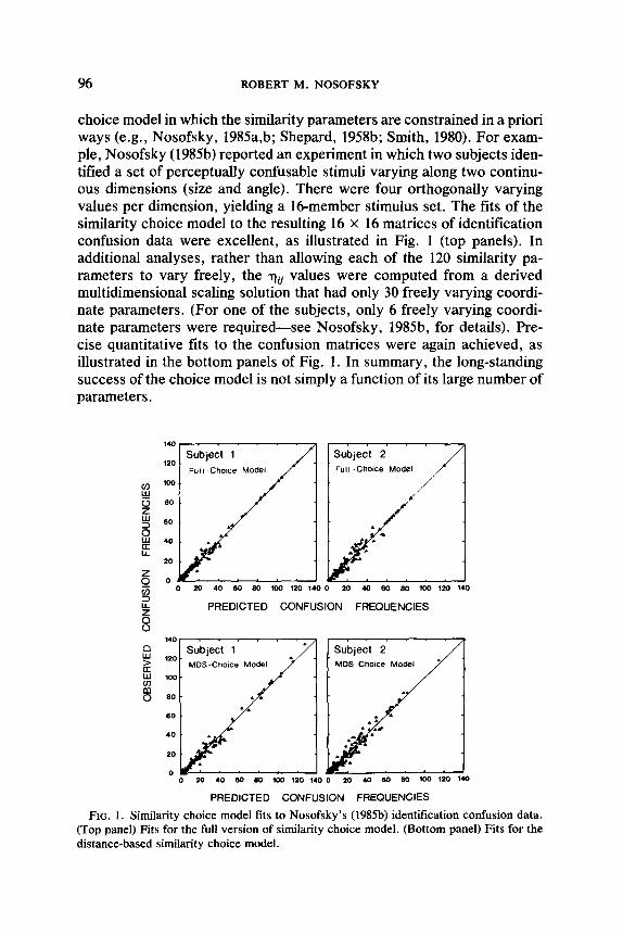
choice model in which the similarity parameters are constrained in a priori ways (e.g., Nosofsky, 1985a,b; Shepard, 1958b; Smith, 1980). For example, Nosofsky (1985b) reported an experiment in which two subjects identified a set of perceptually confusable stimuli varying along two continuous dimensions (size and angle). There were four orthogonally varying values per dimension, yielding a 16-member stimulus set. The fits of the similarity choice model to the resulting 16 x 16 matrices of identification confusion data were excellent, as illustrated in Fig. 1 (top panels). In additional analyses, rather than allowing each of the 120 similarity parameters to vary freely, the rtii values were computed from a derived multidimensional scaling solution that had only 30 freely varying coordi- nate parameters. (For one of the subjects, only 6 freely varying coordi- nate parameters were required-see Nosofsky, 1985b, for details). Pre- cise quantitative fits to the confusion matrices were again achieved, as illustrated in the bottom panels of Fig. 1. In summary, the long-standing success of the choice model is not simply a function of its large number of parameters.

z 0 20 40 60 en 1M) 120 1.0 0 20 40 Bo 8.3 100 120 MO

? PREDICTED CONFUSION FREQUENCIES PREDICTED CONFUSION FREQUENCIES

MDS-Choce Model

PREDICTED CONFUSION FREQUENCIES

FIG. 1. Similarity choice model fits to Nosofsky’s (1985b) identification confusion data. (Top panel) Fits for the full version of similarity choice model. (Bottom panel) Fits for the distance-based similarity choice model.


Many of the confusion matrices that are accurately fitted by the similarity choice model are highly asymmetric. How can a model that assumes symmetric similarity accurately predict asymmetric confusions? The answer lies in the bias parameters (bJ that are part of the model. Generally speaking, if the bias associated with itemj is larger than the bias associated with item i, then i will tend to be confused with j more than the reverse. (Actually, there are two forms of bias in the model, with only one form being reflected by the bj parameters-the other form of bias will be considered shortly.)

The thesis of the present article is that many phenomena that have been characterized in terms of “asymmetric similarity” may be alternatively characterized in terms of differential “bias.” The emphasis in the article is on perceptual classification data, but the ideas are extendable to con- ceptual similarity judgments. Following previous investigators (e.g., Kruskal & Wish, 1978), I use the neutral term “proximity” data in refer- ring to the wide variety of “similarity” data of interest, including direct judgments, identification confusions, same-different errors, and so forth. The main question addressed concerns the extent to which asymmetric proximities can be characterized in terms of symmetric similarity together with differential bias. The influence of bias on other aspects of proximity data besides asymmetry is also discussed.

The idea that asymmetric proximity data are reflecting differential bias is not new, and forms part of the mathematical psychology and statistical literature (e.g., Bishop, Fienberg, & Holland, 1975; Constantine & Gower, 1978; Gower, 1977; Holman, 1979; Shepard, 1957; Smith, 1980, 1982). Yet, the idea has not infiltrated the cognitive psychology main- stream at present. Accordingly, a central goal of this article is one of communication, which is vital given the fundamental importance of similarity in psychological research.

Similarity and Bias, Stimuli and Responses

To begin, it is important to formalize what we mean by similarity and bias. Similarity is a fundamental construct describing a relation between two objects. Formally, it is a function of two variables, which we express as s(i, 1). It makes no sense to speak of the “similarity of i,” although one can speak of the similarity of i to itself, s(i, i). At issue in this article is whether or not similarity can be assumed to be a symmetric relation, with s(i, j) = so’, i).

Whereas similarity is a relation between two objects, bias is defined in this article to be a function of only a single object i, which we express as b(i).

In most experimental situations, one speaks of stimulus similarity and of response bias. That is, similarity is viewed as a relation between stim-


uli, whereas bias is a characteristic pertaining to responses. Independent of the stimulus that is presented, people may have prior biases to use certain responses, e.g., due to payoffs, knowledge of prior probabilities, and so forth (Green & Swets, 1966; Lute, 1963).

The present article suggests a reconceptualization, in which the constructs of similarity and bias are viewed as being orthogonal to stimuli and responses. Thus, one can speak of both stimulus similarity and response similarity, and of both stimulus bias and response bias.

Clearly, just as stimuli have differing degrees of similarity to one another, so do responses. Although in most perceptual classification paradigms the stimuli are confusable and the responses are highly distinctive, the reverse methodology can be used. For example, Shepard (1958b) conducted an experiment in which subjects indicated response assign- ments for highly distinctive symbols by positioning a rod along confusable locations on a unidimensional continuum.

Likewise, it seems sensible to speak of stimulus bias. For example, a particular stimulus may be highly salient in perception or memory, be easily encoded, be easily attended, and so forth. These properties pertain to individual stimuli, not to relations between stimuli, and therefore may be better characterized as biases than as similarities. The intuition is that, independent of the stimulus that is actually presented, there may be prior biases to perceive or remember certain stimuli-not simply to use the responses associated with them.

In many situations it is difficult to determine whether forms of bias arise from the decision/response side of the information processing system or from the perception/memory side. In this article numerous situations are reviewed that appear more easily interpretable in terms of stimulus bias than in terms of response bias.

The interpretation of asymmetric proximities in terms of differential bias-whether response-related or stimulus-related-has a long history. Indeed, in the original formulation of the similarity choice model, Shepard (1957) distinguished between confusability based on stimulus and response processes, and also suggested “. . . it may be that apparent violations of distance symmetry can always be traced to some factor, like familiarity, which pertains to individual (rather than to pairs of) stimuli” (Shepard, 1957, p. 336). It is also of interest to note that although in the modem perceptual classification literature the bias terms in the choice model are uniformly termed “response bias” parameters, Shepard (1957) originally referred to them as “stimulus weights.”

The emphasis in this article on stimulus bias may also be viewed as recapitulating a recurrent theme in the work of Garner and his associates (e.g., Gamer, 1970, 1974; Garner & Clement, 1963; Pomerantz & Gamer, 1973), who have pointed repeatedly to the importance of the individual


stimulus in information processing. In Garner’s work, individual stimuli are viewed as varying in their goodness, with good stimuli being processed more efficiently than poor ones. His argument has not been that interitem similarities are unimportant, but rather that complete models of information processing need to incorporate the roles of both interitem similarities and individual stimulus properties. A main suggestion in this article is that models of proximity data that incorporate properties of the individual stimulus may not require recourse to the positing of “asymmetric similarities. ”

Organization of the Article

The article is organized as follows: In Part 1, I review a mathematical model proposed by Holman (1979) that describes asymmetric proximities in terms of a symmetric similarity function and bias functions on the individual items. This symmetric similarity and bias model generalizes some well-known models that account for asymmetric proximity data, although the role of “bias” in these models is not always widely recog- nized. Consideration is also given in Part 1 to multidimensional scaling approaches that are supplemented by stimulus bias terms. In Part 2, I review and integrate a wide variety of empirical phenomena involving asymmetric patterns of classification data that are interpretable in terms of differential bias. The emphasis is on the potential role of stimulus bias as opposed to response bias. Finally, Part 3 illustrates hypothetical and empirical patterns of asymmetric proximity data that are not interpretable in these terms.

1. DESCRIPTIVE MODELS OF ASYMMETRIC PROXIMITY INCORPORATING SIMILARITY AND BIAS

Additive Similarity and Bias Model

Holman (1979) presented a series of hierarchically organized models for describing asymmetric proximities among stimuli. These models incorporate a symmetric similarity function and bias functions on the individual items. I start the discussion with one of the stronger models that he presents, but it should be emphasized that more general models are possible. According to what I will refer to as the additive similarity and bias model, the proximity of stimulus i to stimulus j [p(i, J] is given by

kG 39 = F[s(i, 59 + 49 + 491, (2)

where F is an increasing function, s(i, 5) is a symmetric similarity function, and r and c are bias functions on the individual objects. Proximity data are typically arranged in matrices in which the rows correspond to the first object in the pair and the columns to the second object. For example, in


an identification confusion matrix, the cell in row i and column j would give the probability with which stimulus i was identified as stimulusj. The function r(i) in Eq. (2) gives the “row” bias for item i, and the function c(j) gives the “column” bias for item j.

Special cases. A number of well-known models that have been applied successfully to account for asymmetric proximity data are closely related to the additive similarity and bias model. Krumhansl (1978) proposed a distance-density model to account for asymmetric proximities and related phenomena. The distance-density between items i and j [d(i, j)] in a multidimensional space is given by

ci(i, 11 = 8d(i, 1) + d(i) + f380, (3)

where d(i, j] is the symmetric distance between i and j, 6(i) is the “density” associated with item i in the psychological space, and 8, IX, and p are weighting factors. Asymmetries arise when the conditions OL # p and 6(i) # S(j) are simultaneously satisfied. With suitable functions for trans- forming distances into proximities, Krumhansl’s distance-density model can be viewed as a special case of the additive similarity and bias model. For example, if the proximity between i and j is given by exp[ -&, 111, then

Ai, 59 = exp[ - Wi, 531 exp[ - 01Wl exp[ - PWI. (4)

This is a special case of Eq. (2) in which F(r) = exp(t), s(i, ~1 = - tkf(i, ~1, r(i) = - c&(i), and C(Z) = - P&(Z).

It is critical to realize that Krumhansl (1978) gave an explicit psychological interpretation to the bias terms, namely, that they reflect “density” in a psychological space. Although density may (or may not; see Cotter, 1987) be one factor that affects bias, there are numerous other possible determinants, many of which will be discussed in this article. The approach taken here is to view the additive similarity and bias model as a general descriptive framework, with the problem of uncovering psychological process interpretations of the bias and similarity terms then being left for further inquiry and discovery.

Tversky (1977) proposed a highly influential similarity model based on feature matching, in which the proximity of item i to item j is given by

p(i, 59 = mm n 4 - c-&Z - 4 - PflJ - 1)1, (5)

where F is an increasing function; Z and J are the feature sets that com- pose items i and j; Z fl J denotes the set of features common to Z and J; Z - J and J - Z denote the features that are distinctive to Z and J, respectively; f is a measure function of the features; and 8, a, and p are weighting factors. Asymmetries arise when the conditions flZ - .Z) # f(J - Z) and cx # l3 are simultaneously satisfied. As noted by Holman (1979),


when the measure functionfis taken to be an additive set function [so that flZ U J) = AZ) + f(J) when Z and .Z are disjoint], then Tversky’s feature model can be rewritten as

P(i, 59 = F[@ + a + PI AZ f-l .o - %m - Pfol. (6)

This is a special case of the additive similarity and bias model, where s(i, 3’) = (13 + (Y + p) f(r n .Z), r(i) = -oLf(Z), and ~$1 = - l3fl.Z). In other words, the asymmetric proximities predicted by the additive version of Tversky’s feature matching model are characterizable in terms of a symmetric similarity function and bias functions on the individual stimuli (see Smith, 1982, for a related analysis). According to the additive version of Tversky’s model, the biases associated with the individual stimuli measure the salience of the stimuli’s features. Again, note that the salience of a stimulus’ features is a property of that particular stimulus, not of relations between stimuli. Therefore, it seems well characterized as a stimulus bias. Although the additive version of Tversky’s model is most often applied, it should be acknowledged that less restrictive, nonadditive versions of his model are not in general decomposable into symmetric similarity and individual bias components (Holman, 1979, p. 7).

As discussed in the introduction, one of the classic models for predicting identification confusion data is the similarity choice model [Eq. (l)]. Holman (1979) noted that the similarity choice model is also a special case of the additive similarity and bias model [Eq. (2)], where s(i, I] = log Q, r(i) = -log Cbkqik, co) = log bj, and F(t) = exp(t). Earlier in the discussion, I noted that there are two forms of bias in the choice model, only one of which is directly reflected by the bj parameters. The bj parameters are column biases. The other form of bias in the choice model is row bias, i.e., the expression in the denominator of Eq. (1). Defining the value bjqti as the “strength of association” from object i to objectj, then the row bias measures the total strength of association between a given item and all other items in the set. Note that even if all column biases are equal, the row bias values will generally not be equal, because Q = -qji does not imply that Zqik = Cqjk. Thus, even without use of the column bias parameters, the symmetric-similarity choice model will still predict asymmetric confusions. Getty, Swets, Swets, and Green (1979, Fig. 1) have provided a useful illustration of this point.

Self-proximity. A question closely related to asymmetric proximity re- gards differences in self-proximities. For example, in a similarity judgment task, a given item may be rated as having greater self-similarity than another item (Gati & Tversky, 1982). Or, in a same-different task, the percentage of correct “same” responses may vary across items (Roth- kopf, 1957).

According to the additive similarity and bias model, differences in self-


proximity may arise because of differential bias associated with the individual items. Assuming that self-similarities are equal, the self-proximity for itemj will be greater than the self-proximity for item i whenever r(~] + co > r(i) + c(i).

For the general version of the additive similarity and bias model, there is no necessary relationship between the direction of asymmetric proximities and the magnitude of self-proximities. That is, the relationpo, j) > p(i, i) in and of itself implies nothing about the relation between p(i, 1) and pG, i). However, for some of the special cases of the additive similarity and bias model (as they are currently articulated), specific implications are involved.

According to Tversky (1977), when people rate the similarity of item i to item j (a directional judgment), the weight cx in Eq. (6) is greater than the weight B because item i serves as the subject of the comparison. Thus, the rated similarity of item i to item j will exceed the rated similarity ofj to i wheneverfo >flZ). In other words, the less salient stimulus is rated as more similar to the salient stimulus than the reverse. But ifA. >fo, then it is also the case that the self-proximity for item j will exceed the self-proximity for item i, i.e., the self-proximity for the salient stimulus will exceed the self-proximity for the nonsalient stimulus. To summarize, in Tversky’s approach to modeling similarity judgments, the relation p(i, J) > p(j, i) implies the relation p(j, j) > p(i, i).

The opposite state of affairs exists for Krumhansl’s distancedensity model. Following Tversky (1977), Krumhansl(l978) assumed that in judg- ing the similarity of i to j, the weight cx in Eq. (3) is greater than the weight p. In this case, the distance-density from i to j exceeds the distance density from j to i whenever 6(i) > S(J). Thus, because similarity is a decreasing function of distance-density, the similarity of i to j would exceed the similarity ofj to i whenever So) > 6(i). In other words, an item in an isolated region of the space is rated as more similar to an item in a dense region than the reverse. But if S(j) > 6(i), then the distance-density ofj to itself exceeds the distance-density of i to itself, and so the self- proximity for i exceeds the self-proximity for j. To summarize, in Krum- hansl’s approach to modeling similarity judgments, the relation p(i, ~3 > p(j, i) implies the relation p(i, i) > p(j, J), which is opposite to the prediction stemming from Tversky’s (1977) model.

To my knowledge, this sharp contrast between Tversky’s (1977) and Krumhansl’s (1978) models regarding implication relations between asymmetric proximities and self-proximities has not been noted in previous work. With regard to similarity judgments, it seems likely that Tver- sky’s model would be favored. Tversky and Gati (1978) obtained systematic evidence that less prominent countries (e.g., North Korea) were rated as more similar to prominent countries (e.g., China) than the reverse. Ac-


cording to Krumhansl’s (1978) analysis, China would be located in a dense region of psychological space. Therefore, it should have lower rated self-similarity than North Korea. Although I am aware of no published data that bear directly on this issue, it seems likely that the reverse empirical result would be observed. Evidence consistent with this con- jecture is provided by Gati and Tversky (1982), who showed that increasing the prominence of schematic-face stimuli by adding common features to them increased their rated self-similarity. Also, faces with fewer features were rated as more similar to faces with many features than the reverse.

Although Tversky’s model may be favored in the domain of similarity judgments, later in this article I will review some patterns of same- different judgment data that favor Krumhansl’s model (see also Krum- hansl, 1982). The important point is that although differential stimulus bias may influence both asymmetric proximities and self-proximities, the precise manner in which it operates varies with experimental conditions.

Stimulus Bias, Multidimensional Scaling, and Tversky’s Feature-Contrast Model

Multidimensional scaling (MDS) theory is a classic approach to representing proximity data (Shepard, 1980). In MDS models, objects are represented as points in a multidimensional space, and proximity is assumed to be a decreasing function of distance in the space, p(i, j) = g[d(i, ~11, where g is a decreasing function. Traditional MDS models compute distance using versions of the Minkowski power model formula,

(7)

where xim is the psychological value of stimulus i on dimension m, and M is the number of dimensions. Standard values of r are r = 1, the city-block metric; and r = 2, the Euclidean metric (e.g., Attneave, 1950; Gamer, 1974; Shepard, 1964, 1987).

As elucidated by Tversky and his colleagues (e.g., Gati & Tversky, 1982; Krantz & Tversky, 1975; Tversky, 1977; Tversky & Gati, 1978, 1982; Tversky & Hutchinson, 1986), numerous assumptions that underlie traditional MDS models are not upheld in sets of proximity data, with the existence of asymmetric proximities and differences in self-proximities forming only a subset of the problems. Elegant accounts of these problematic phenomena have been provided within the framework of Tver- sky’s (1977) feature-contrast model. The purpose of the present section is


to consider the relation between the feature-contrast model and MDS models that are supplemented with stimulus bias terms.

In the following it is assumed that the stimulus set is constructed from M “additive” features, with each feature being either present or absent. (Stimulus sets constructed from “substitutive” features can be given an additive feature representation, so the following analysis holds for these sets as well.) An object i is represented as a vector Z = (Ii, Z2, . . . , I&, with each Z, equal either to pm (indicating presence of feature m) or zero (indicating absence). Using this notation, the additive version of Tver- sky’s (1977) feature-contrast model can be written as

pG9.8==Fe+a+P) C flL)-~~AZm)--P~flJm). [ t?l:I,=J m m m 1

Q-3)

(The index m:Z,,, = J,,, indicates that the summation is over all features that are in both Z and J.)

A bias-supplemented MDS model for representing proximities among these stimuli can be formulated as follows:

p(i, j) = F[utii) + vc0 - wd(i, 311, (9)

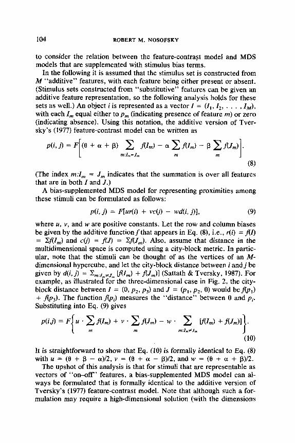
where u, v, and w are positive constants. Let the row and column biases be given by the additive functionfthat appears in Eq. (8), i.e., r(i) = AZ) = XflZ,,J and C(Z) = fl.Z) = EflJ,). Also, assume that distance in the multidimensional space is computed using a city-block metric. In particular, note that the stimuli can be thought of as the vertices of an M- dimensional hypercube, and let the city-block distance between i andj be given by d(i, 11 = &rl,+Jm [f(Z,J + fl.Z,,,)] (Sattath & Tversky, 1987). For example, as illustrated for the three-dimensional case in Fig. 2, the city- block distance between Z = (0, p2, p3) and .Z = (pi, p2, 0) would be&,) + &+). The function f(pi) measures the “distance” between 0 and pi. Substituting into Eq. (9) gives

It is straightforward to show that Eq. (10) is formally identical to Eq. (8) with u = (0 + l3 - CX)/~, v = (fl + OL - p)/2, and w = (6 + cx + j3)/2.

The upshot of this analysis is that for stimuli that are representable as vectors of “on-off’ features, a bias-supplemented MDS model can always be formulated that is formally identical to the additive version of Tversky’s (1977) feature-contrast model. Note that although such a formulation may require a high-dimensional solution (with the dimensions

BIAS AND ASYMMETRIC SIMILARITY

uJ,P2’0)

yq

? I 9 1’ 2’

I

(0.0.P3) A- /

- - -- - - --(

/

/

/ /

105

) (P1’P*‘P+

(P1’O,O)

FIG. 2. Three-dimensional cube for illustrating city-block distances between featural stimuli. The right, top, and back faces of the cube represent the presence of features 1, 2, and 3, respectively.

being binary-valued), there is no logical necessity that MDS solutions consist of only a few continuous dimensions. From this perspective, the additive version of Tversky’s (1977) feature-contrast model can be viewed as providing a theory of the stimulus bias terms in bias-supplemented MDS models.

It follows from the preceding analysis that any of the phenomena that proved problematic for traditional MDS models, but which are well accounted for by the additive version of Tversky’s feature-contrast model, are in principle explicable in terms of bias-supplemented MDS models. An interesting example involves nearest-neighbor analyses of proximity data (e.g., Tversky & Hutchinson, 1986). The relation “i is the nearest neighbor ofj” means that, among all items in the stimulus set, item i is the most proximal to itemj. The centrality of an item i with respect to a given set S is defined as the number of elements in S whose nearest neighbor is item i. The centrality statistic is important because it places severe constraints on traditional MDS models of proximity data. For example, it can be shown that in a two-dimensional Euclidean scaling solution, a given item can be the nearest neighbor of no more than five objects.

Tversky and Hutchinson (1986) reported a data set collected by Mervis, Rips, Rosch, Shoben, and Smith (1975) in which this centrality constraint was severely violated. The items in the stimulus set had a hierarchical structure. In particular, Mervis et al. (1975) collected relatedness ratings


for names of 19 different fruits plus the category name fruit. The relatedness ratings indicated that the category name fruit was the nearest neighbor of all but two instances in the 20-item set. Although the category name was centrally located in a two-dimensional Euclidean scaling solution for the relatedness ratings data (see Tversky & Hutchinson, 1986, p. 6), it nevertheless was the nearest neighbor of only two points in the spatial configuration, The Euclidean model was able to account for only 47% of the linearly explained variance in the proximity data.

The main alternative model that Tversky and Hutchinson (1986) compared to the Euclidean spatial model was the additive tree representation (Sattath & Tversky, 1977). However, they also discussed a hybrid model (Carroll, 1976) that combined spatial and hierarchical components. In Carroll’s hybrid model, the (symmetric) dissimilarity between items i and j is given by

D(i, 51 = d(i, 31 + h(i) + W, (11)

where d(i, j) is the distance between i and j in a common Euclidean space, and h(i) and h(j) are hierarchical components reflecting the distance from i and j to the common space. These hierarchical components are examples of stimulus biases.

Use of the hierarchical components dramatically improved the fit of the Euclidean scaling model to the relatedness ratings data, increasing the percentage of linearly explained variance from 47 to 91%. (A three- dimensional Euclidean scaling solution with the same number of parameters as the hybrid model accounted for only 54% of the variance.) Thus, the stimulus bias terms were critical for achieving an accurate quantitative fit to the data.

The hybrid model accounted for the high centrality of the category namefruit by making its hierarchical component very small relative to the hierarchical components associated with the category instances. Thus, any distance involving h(fruit) tended to be relatively small, so fruit was the nearest neighbor of most objects in the set.

Summary

In summary, a variety of extant models for describing asymmetric proximities are special cases of a model incorporating a symmetric similarity function and bias functions on the individual objects (Holman, 1979). This symmetric-similarity and bias model can also characterize differences in self-proximities. Implication relations between the direction of asymmetric proximities and self-proximities were considered and shown to place constraints on some of the special cases of the similarity and bias model. Finally, it was noted that the additive version of Tver-


sky’s (1977) feature-contrast model can be viewed as a special case of bias-supplemented MDS models.

2. STIMULUS BIAS AND CLASSIFICATION DATA: A REVIEW AND INTEGRATION

The aim in this section is to review and integrate a variety of phenomena involving classification data that are well characterized by models incorporating a symmetric similarity function and bias functions. Al- though the emphasis is on asymmetries, the role of bias in intluencing other aspects of classification data is also considered. A key point in this section is to illustrate that in many cases the biases appear to be reflecting stimulus properties as opposed to pure response processes.

It is worth reemphasizing that “bias” is defined in this article in a very general sense, namely, as a function of an individual object. In the up- coming review, therefore, numerous diverse phenomena come under the unified heading of bias. In each of the cases considered, it is argued that in addition to the role of similarity relations, properties of individual objects are exerting dramatic impact on patterns of classification performance. Moreover, across domains, the joint impact of these similarities and individual item biases is modeled in essentially the same way. I make no claim that the specific psychological processes and mechanisms underlying these diverse phenomena are the same-only that they can be given a common abstract characterization in terms of symmetric similarities together with individual item biases.

On several occasions in the review, alternative models are compared on their ability to fit matrices of identification and same-different confusion data. The models are often evaluated using the likelihood ratio statistic G*, given by

(W

wherefi is the observed frequency in cell i of the matrices, and x is the maximum-likelihood predicted frequency (Bishop et al., 1975). The statistic G* is distributed asymptotically as x2 with degrees of freedom equal to the number of freely varying data points minus the number of free parameters. A restricted version of a model arises when some of its parameters are constrained on a priori grounds. Let G*(F) denote the fit for a full model under consideration, and let G*(R) denote the fit for a restricted version of the model. Assuming that the restricted model is correct, the difference G*(R) - G*(F) is distributed asymptotically as x2 with degrees of freedom equal to the number of constrained parameters. If the


difference in G* is statistically significant, then one would conclude thal some of the parameters were constrained inappropriately.*

A. Density and Identification Confusions

As noted in Part 1, Krumhansl’s (1978) distance-density model predicts that an item in a sparse region of a space will be judged as more similar to an item in a dense region than the reverse. Krumhansl reviewed a wide array of similarity data that supported this prediction. When Krumhansl’s model is linked to the similarity choice model [Eq. (I)], however, it makes a rather surprising and counterintuitive prediction with regard to identification confusion data. Following Shepard (1958a, 1987), assume that similarity between items i and j is an exponential decay function of their distance in psychological space. Then the “similarity-density” between items i and j would be given by

flu = exp[ - 8d(i, ~11 exp[ - &3(i)] exp[ - l3Sb)]. (13)

Following Takane and Shibayama (1985), we now substitute the expression for Fiji into the choice model [Eq. (l)]. The term exp[ - c&(i)] cancels out of numerator and denominator and we obtain

P@jlSi) = bjid bj exp[ - Bd(i, ~91 exp[ - P WI s = c bk exd-8dk Ml exp[- PWI

k k

bjhij =C’

k

(14)

where qij = exp[ - 8d(i, 311 and b; = bj exp[ - p&J]. Thus, the asymmetric portion of flij computed from Krumhansl’s model is absorbed by the column bias parameters of the choice model.

In other words, if Krumhansl’s ideas about the role of density are correct, then a portion of the choice model column bias parameters should be reflecting stimulus density. Furthermore, it can be seen that as the density around itemj decreases, the column bias bj* should increase. This means that in an identification experiment, an item in a dense region of a space would tend to be confused with an item in a sparse region more

’ Most of the ensuing statistical analyses should be considered as merely illustrative, however, because various underlying assumptions of the tests are often not met (e.g., data may be averaged over conditions and subjects, or some cell frequencies may be too small for the G* statistic to reliably follow the x2 distribution).


than the reverse-precisely the opposite prediction that is made for patterns of asymmetric similarity judgments!3

Shepard (1958b) and Nosofsky (1987) provide examples of choice model analyses of identification confusion data that support this density prediction. In Nosofsky’s (1987) study, subjects learned to identify a set of 12 Munsell colors varying in brightness and saturation. The cumulated learning matrix that was obtained is given in Table 1. The choice model was used to fit the learning data, with the assumption that the similarity parameters were functionally related to distances in a two-dimensional psychological space (Shepard, 1957, 1958b). Specifically, each stimulus was represented as a point in a two-dimensional space; distance between stimuli was computed using a Euclidean metric; distance was transformed into a similarity measure using an exponential decay function; and the derived similarities were then substituted into Eq. 1 to predict the identification confusions in Table 1 (see Nosofsky, 1987, pp. 94-96, for details of the analysis).

The MDS solution derived by fitting this distance-based choice model to the identification data is illustrated in Fig. 3. The circles surrounding each stimulus point represent the estimated biases, with the magnitude of the bias being an increasing function of the size of the circle. This set of stimulus coordinates and biases together accounted for 99.8% of the total variance in the 144-cell identification confusion matrix, and for 97.4% of the error variance (i.e., the entries in the off-diagonal cells taken alone). Inspection of Fig. 3 reveals that the biases associated with stimuli in isolated regions of the space tend to be larger than the biases associated with stimuli in dense regions, as predicted by Krumhansl’s density hypothesis. The correlation between the estimated bias for each stimulus and the average similarity of the stimulus to other members in the set was r = - .75 (p < .Ol).

To illustrate the role of the bias parameters in reflecting asymmetries in the identification confusions (see Table 1 and Fig. 3), note that Color 8 was called Color 10 89 times, while Color 10 was called Color 8 only 50 times; Color 3 was called Color 1 152 times, while Color 1 was called Color 3 only 82 times; and Color 9 was called Color 12 69 times, while

3 This prediction about the direction of asymmetries should not be stated so strongly. The predicted direction of asymmetries depends on the relative magnitudes of the column bias parameters. It is straightforward to verify that if all column biases are equal, then the row bias terms in the choice model lead to the prediction that items in sparse regions are confused with items in dense regions more than the reverse (e.g., see Nosofsky, 1985b, p. 416). Thus, the column biases and row biases exert competing influences. The critical prediction stemming from Krumhansl’s (1978) hypothesis is simply that the column biases will be larger for items in isolated regions of psychological space.


SATURATION FIG. 3. MDS solution derived by fitting the distance-based similarity choice model to

Nosofsky’s (1987) color identification data. Estimated biases are roughly linearly related to size of enclosing circles.

Color 12 was called Color 9 only 27 times. Confusions tend to travel from dense regions to sparse regions more than the reverse, as reflected by the bias parameters. Likelihood-ratio tests indicated that the bias parameters departed significantly from a uniform pattern (p < .OOl).

Shepard (1958b) observed a similar relation between estimated bias and spatial density. In a choice model analysis of a set of identification confusion data using nine Munsell colors, the correlation between the bias terms and average similarity of an item to the remaining members of the set was r = - .88 b < .Ol). He also conducted a choice model analysis of a set of confusion data in which subjects identified a set of nine geometric forms varying only in size. The estimated biases were largest for those items lying near the extremes of the unidimensional scaling solution, i.e., those items in the least dense regions (see Shepard, 1958b, Table 1). The bias-“average similarity” correlation was r = - .89, p < .Ol. Keren and Baggen (1981) reviewed a choice model analysis of a set of alphabetic confusion data reported by Gilmore, Hersh, Caramazza, and Griffin (1979), and noted a bias-“average similarity” correlation of r = - .73, p c .Ol.

Unfortunately, it is unclear in the context of these identification experiments whether the pattern of bias is reflecting the property of stimulus density per se or a response strategy. On the one hand, in Nosofsky’s (1987) and Shepard’s (1958b) experiments, stimulus-response assign- ments were randomized for each subject. Thus, the biases are clearly not reflecting subjects’ preferences for using certain labels as responses. On


TABLE 1 Cumulated Stimulus-Response Learning Matrix Obtained in Nosofsky’s (1987) Color

Identification Study (Adapted from Table 1 in Nosofsky, 1987)

Response

Stimulus 1 2 3 4 5 6 7 8 9 10 11 12 -

1

2

3

4

5

6

7

8

9

10

11

12

665 17 82 13 663 19 90 14

21 670 38 121 25 669 29 124

152 28 453 37 135 30 460 35

12 156 35 581 21 146 38 577 73 8 63 12 79 9 75 11 30 15 85 42 30 19 80 40 10 17 10 38 8 15 15 40

14 9 35 20 20 7 30 9

6 5 26 13 9 9 17 17 5 7 8 7 7 4 7 5 3 3 8 3 5 4 6 5 4 5 10 0 5 4 6 5

Cumulated 63 19 64 21 9 20

10 18 82 78 90 77 19 46 13 42

552 32 533 44

55 466 54 471 12 54 11 48 77 64 87 56 16 65 17 67 14 16 20 9

7 6 9 11 7 2 7 10

4 20 13 14 4 7 6 18 7 9 5 5

12 10 7 1 3 6 13 8 8 5 5 4 7 39 18 10 7 5

13 37 15 11 7 6 36 12 14 2 1 4 36 12 17 6 6 6 13 100 24 18 13 9 8 93 13 33 10 7

46 70 59 12 15 19 42 74 60 15 15 12

616 17 117 4 9 15 621 18 100 8 16 20

18 513 28 89 33 14 13 539 34 70 32 17

101 48 507 10 52 69 99 49 517 16 48 52

9 50 8 767 22 5 5 42 9 770 28 12

11 37 28 48 594 172 11 28 29 39 599 174 18 22 27 13 216 591 14 18 35 18 200 592

Note. Top line in each row, observed confusion frequencies; bottom line, predicted confusion frequencies.

the other hand, Smith (1978) has noted that different patterns of response bias will alter the choice model’s predictions of percentage of correct identifications. It turns out that it is an optimal strategy for subjects to bias their responses toward stimuli in more isolated regions of psychological space (see Smith, 1980, p. 151, for an example), although the expected changes in percentage of correct identifications are often ex- ceedingly small. Clearer evidence that the bias parameters may be reflecting stimulus properties rather than response strategies is provided in the next section, where we examine categorization rather than identification.

B. Frequency and Category Typicality By categorization, I mean a choice experiment in which people classify


items into groups rather than identifying them with unique labels. Be- cause many stimuli are assigned the same response in categorization, it becomes possible to decouple the influence of stimulus and response biases.

The similarity choice model for identification has been extended by Medin and Schaffer (1978) and Nosofsky (1984, 1986) so as to apply to categorization. According to the categorization model, the strength of making a Category J response given presentation of Stimulus i is found by summing the similarity of Stimulus i to all items j belonging to Category J and then multiplying by the response bias for Category J. This strength is then divided by the sum of strengths for all categories to determine the conditional probability with which Stimulus i is classified in Category J:

BJ~ 'Xi

P(R$i) = e t

K ( >

(15)

where BJ is the Category J response bias. Successful quantitative applications of the categorization model have been demonstrated in numerous experiments (e.g., Busemeyer, Dewey, & Medin, 1984; Estes, 1986; Me- din & Schaffer, 1978; Medin & Smith, 1981; Nosofsky, 1984, 1986, 1987, 1988, 1989a).

A more genera1 version of the categorization model incorporates stimulus bias terms (e.g., Nosofsky, 1987, 1988):

These stimulus biases (bj) have figured importantly in some experimental conditions. An example is an experiment reported by Nosofsky (1988) in which people learned to classify a set of 12 Munsell colors into two categories. The category structure is illustrated in Fig. 4. I will refer to the set of stimuli enclosed by circles as the target category, and to the set of stimuli enclosed by triangles as the contrast category. The colors were identical to those used in Nosofsky’s (1987) identification learning study that was discussed in the previous section. Recall that the MDS solution for the colors was derived on the basis of confusion errors observed during identification learning (compare Figs. 3 and 4). This same MDS solution was used for computing similarities among items in the present categorization experiment.


SATURATION FIG. 4. Category structure tested by Nosofsky (1988). Stimuli enclosed by circles, mem-

bers of target category; stimuli enclosed by triangles, members of contrast category.

After a training phase in which people learned the category assignment for each color, a transfer phase was conducted. In one task people gave ratings of how “typical” or how “good an example” each color was of its respective category, whereas in a second task typicality paired-comparison judgments were collected.

The major experimental manipulation was that across conditions, individual colors were presented with high frequency during training. For example, in one condition Color 2 was presented roughly five times as often as any of the other colors, whereas in two other conditions Colors 7 and 6 were presented with high frequency. The experimental manipulation had a dramatic influence on people’s classification confidence and typicality judgments. First, relative to a baseline condition in which all colors were presented with equal frequency, classification confidence and typicality ratings for the high frequency colors increased substantially. Indeed, a crossover effect was observed, in which Color 2 was rated as the best example of the target category when it was presented with high frequency, while Color 7 was rated as the best example of the target category when it was presented with high frequency. More interestingly, classification confidence and typicality ratings also increased for category members that were similar to the high-frequency exemplars. For example, in the condition in which Color 2 was presented with high frequency, typicality ratings increased substantially for its neighbor Color 4 (see Fig. 4). Finally, typicality ratings decreased for members of the contrast cat-


egory that were similar to the high-frequency exemplars. For example, typicality ratings for Color 8 of the contrast category decreased when Color 6 of the target category was presented with high frequency (see Fig. 4).

A fair metaphorical summary of the results is that the high-frequency stimulus acted as a “magnet” in the psychological space, drawing nearby stimuli toward it. This property of the high-frequency stimulus seems well characterized as a stimulus bias. Indeed, good quantitative fits to the classification and typicality ratings data were achieved using the stimulus- bias version of the categorization model [Eq. (16)], with the assumption that the stimulus biases were proportional to the relative frequencies of the stimuli. This frequency-sensitive model accurately reflected the joint, interactive roles of interitem similarities and individual item frequencies in influencing the graded structure of the categories.

It is critical to realize that the frequency manipulations for the individual stimuli led to modifications in local classification probabilities, not to global changes in overall category response bias. When Color 2 was presented with high frequency, classification behavior changed for Color 2 and its neighbor Color 4, but not for the other members of the category. Not surprisingly, therefore, the version of the categorization model without the stimulus bias terms [Eq. (15)] could not provide an accurate quantitative account of the data-simply varying the category response bias parameter across conditions predicts major changes in classification behavior for all items in the set. Thus, the categorization paradigm provides evidence for the influence of individual stimulus biases as opposed to purely response bias processes.

C. Natural Prototypes in Categorization

In the previous section I discussed an experimentally induced stimulus bias that arose from manipulations in learning conditions. Other forms of stimulus bias may reflect innate aspects of stimulus processing. In her seminal studies of natural categorization, Rosch (1973) argued that many perceptual categories found in the natural world are organized around focal elements called “natural prototypes.” With respect to color and form categories, Rosch (1973, p. 113) proposed that “there are colors and forms which are more perceptually salient than other stimuli in their domains,” and that it is these salient stimuli around which natural categories come to be organized. She tested and found support for the hypothesis that it is easier to learn categories in which the presumed natural prototype is central to a set of variations than it is to learn categories in which a distortion of the prototype is central and the natural prototype occurs as a peripheral member.

The idea that an item functions as a natural prototype provides a


clearcut example of what I have been calling stimulus bias. Properties of the individual stimulus give it a special status that plays a critical role in classification. Furthermore, it can be shown that Rosch’s (1973) result that it was easier for subjects to learn sets of categories in which the natural prototypes were central members is predicted by the stimulus-bias version of the categorization model [Eq. (16)]. The basic intuition is that the “magnetic power” associated with the prototype has optimal intlu- ence when it is centrally located with respect to the other items in the category.

D. Asymmetries Due to Feature Loss and Feature Gain

The identification and categorization paradigms discussed thus far have involved stimuli varying along continuous dimensions. Another common situation is for stimuli to be composed of discrete features that are either present or absent and to induce confusions through use of state or process limitations (e.g., Evans & Craig, 1986; Garner & Haun, 1978; Townsend, Hu, & Ashby, 1980; Townsend, Hu, & Evans, 1984). An example of a state limitation would involve presenting stimuli using short exposure durations, which presumably would tend to lead to feature “loss.” By contrast, process limitation would arise by adding a post-stimulus pattern mask, which presumably would tend to lead to feature “gain.”

Gamer and Haun (1978) provide a simple illustrative example of such a paradigm. All stimuli were composed of a vertical bar with either no horizontal bar added (I), the lower horizontal bar added (L), the upper bar added (r), or both bars added (c). Identification confusion matrices obtained in state-limited and process-limited conditions are shown in Table 2. In the state-limited condition, the direction of errors was from stimuli with more features to stimuli with fewer features. The opposite picture emerged in the process-limited condition.

As is reasonable from inspection of the matrices, Garner and Haun (1978) described the different forms of perceptual limitation as having led to different patterns of asymmetric similarity relations among the items, e.g., in the state-limited condition, stimuli with many features were more similar to stimuli with few features than the reverse. In an analysis of Gamer and Haun’s data, however, Smith (1980) showed that, in both the stated-limited and process-limited conditions, the confusion data were well described by the symmetric-similarity choice model [Eq. (l)]. The choice model predictions are shown along with the observed data in Table 2. By conventional criteria, the predictions would be considered out- standing. The best-fitting parameters and summary fits are reported in Table 3. The biases are in the direction of stimuli with fewer features in the state-limited condition, and in the direction of stimuli with more features in the process-limited condition. In summary, the asymmetric prox-


TABLE 2 Observed Identification Confusion Frequencies for Gamer and Haun’s (1978)

“Feature-Set” Stimuli in the State-Limited and Process-Liited Conditions, Together with the Predicted Frequencies for the Similarity Choice Model

Response

Stimulus I L r c N A. State-limited condition

I 1003.0 147.0 93.0 37.0 1280 1003.0 157.4 94.6 24.9

L 222.0 974.0 38.0 46.0 1280 211.6 974.0 38.6 55.8

r 250.0 76.0 868.0 86.0 1280 248.4 75.4 868.0 88.2

c 125.0 238.0 187.0 730.0 1280 137.1 228.2 184.8 730.0

B. Process-limited condition I 943.0 89.0 102.0 34.0 1168

943.0 98.3 97.2 29.5

L 94.0 1204.0 29.0 129.0 1456 84.7 1204.0 29.2 138.1

r 72.0 27.0 1119.0 142.0 1360 76.8 26.8 1119.0 137.4

c 8.0 77.0 69.0 982.0 1136 12.5 67.9 73.6 982.0

Note. Top line in each row, observed frequencies; bottom line, predicted frequencies. N, total number of stimulus presentations.

imities resulting from feature loss and feature gain are well characterized by a model that uses a symmetric similarity function and bias functions on the individual items.

Nosofsky (in press) noted a formal correspondence between the similarity choice model and an independent feature additiondeletion model. Assume we have a set of stimuli composed from discrete features, with each feature being either present or absent. Because of noise in the perceptual processing system, there is some probability u, that feature m will be “added” (assuming it is not in the actual stimulus) and some probability d, that feature m will be “deleted” (assuming it is in the actual stimulus). Assuming independence, the predicted stimulus- response confusion probabilities that would arise for a powerset of stimuli generated from the features x and y [e.g., the Gamer and Haun (1978) stimuli] is shown in Table 4A. For example, the probability that x is identified as xy is equal to the product of the probabilities that feature x is


TABLE 3 Maximum-Likelihood Similarity Choice Model Parameters and Summary Fits for Garner

and Haun’s (1978) “Feature-Set” Stimuli Confusion Matrices

State-limited condition” I

k= c

Process-limited conditionb

L l- c

Similarity (Q)

L l- c Bias (bj)

,185 .164 .068 .359 .059 .134 .305

.160 .206 .131

.086 ,084 .020 .200 .024 .089 .243

.096 .245 .313

’ G2 = 9.76. b G2 = 7.19.

not deleted and feature y is added, (1 - d&z,,. If the addition-deletion probabilities are highly asymmetric, then the resulting confusion matrix is highly asymmetric, as illustrated in Table 4B. Despite the asymmetries, Nosofsky (in press) proved that for any powerset of stimuli constructed from M features, the independent feature additiondeletion model is a special case of the similarity choice model, with similarity and bias parameters given as follows. Let Z and .Z denote the sets of features composing stimuli i and j, respectively. Then

TABLE 4A Illustration of Independent Feature Addition-Deletion Model for a Powerset of Stimuli

Constructed from Two Features

Response

Stimulus 0 x Y xy

0 (1 - a,) 4 (1 - UJ (1 - 4 ay %$ (1 - a,)

x d, (1 - a,) (1 - 4 (1 - aJ

(1 - 4) ay

Y (1 - a,) d, (1 - a,) (1 - d,)

a, (1 - d,)

xy (1 - 4) d, 4 (1 - d,J (1 - 4 (1 - dy)

Note. a,,,, probability that feature m is added. d,,,, probability that feature m is deleted.


TABLE 4B Illustration of Asymmetric Confusion Matrix Produced by Addition-Deletion Model

kl = .1, d,,, = .4)

Response

Stimulus 0 X Y v

0 810 90 90 10 X 360 540 40 60 Y 360 40 540 60

xy 160 240 240 360

Note. Based on 1000 observations per stimulus.

‘Xi = 7F (1 - a,)(1 - d,) ’

me NZ U J) - (1 n 41

Wa)

and

where b. is the bias for the null stimulus. From Eq. 17, it can be seen that similarity between stimuli is deter-

mined jointly by the number of features that are distinctive to the stimuli and by the switching probabilities for those features. With regard to bias, if the a,,, addition probabilities are large relative to the d,,, deletion probabilities, then bias would tend to be in the direction of stimuli with more features, and vice versa if the deletion probabilities are large relative to the addition probabilities. These biases resulting from perceptual addition and deletion processes again seem well characterized as stimulus biases.

The independent feature additiondeletion model can also be viewed as a particular multidimensional signal detection model (Ashby & Town- send, 1986). For each dimension m, the probability of a “hit” (correctly detecting a signal) is 1 - d,, that of a “false alarm” (incorrectly detecting a signal when noise alone is present) is a,,,, that of a “correct rejection” is 1 - a,, and that of a “miss” is d,. In the model, the hit and false alarm probabilities for individual dimensions are independent of the values that occur on the other dimensions. In the language of Ashby and Townsend (1986), this condition would be satisfied if perceptual independence, perceptual separability, and decisional separability all held. Because this model is a special case of the similarity choice model, it is seen that certain special cases of multidimensional signal detection models


produce patterns of proximity data that are characterizable in terms of a symmetric similarity function and individual item biases.

E. Asymmetric “Same-Different” Confusions

Rothkopf (1957) reported a set of “same-different” confusion data using 36 Morse code signals. Many of the confusions were asymmetric, i.e., a given signal i may have been judged the same as signalj more than signal j was judged the same as signal i. [Signals were presented sequentially, so there is a clear distinction between p(i, 1) and p(j, i).] Also, the percent- ages of correct “same” responses varied; e.g., pair E-E was correctly judged “same” 97% of the time, whereas pair P-P was correctly judged “same” only 83% of the time.

Tversky (1977) and Krumhansl(l978) noted that the general pattern of asymmetries in the Rothkopf (1957) data was consistent with versions of their models of asymmetric similarity. Tversky (1977) considered the Morse code signals in terms of temporal length, and conducted analyses that showed that shorter signals were judged the same as longer signals significantly more than the reverse. This pattern of asymmetry is consistent with his feature-matching model if it is assumed that the first signal serves as the subject of the comparison and the second signal as the referent, and, consistent with his other work, that long signals are more prominent than short signals. Krumhansl (1978) made use of an MDS solution for the signals published by Shepard (1963). She found that signals in relatively isolated regions of the space were judged the same as signals in dense regions more than the reverse. This pattern is consistent with her distance-density model if it is assumed that the first signal serves as the subject of the comparison and the second signal as the referent.

In this section I illustrate an exploratory analysis of the Rothkopf (1957) same-different data using the additive similarity and bias model [Eq. (2)]. The idea is that instead of assuming a priori that the stimulus biases are related to temporal length or stimulus density, I allow the stimulus bias parameters to vary freely and attempt to discover correspondences between the estimated biases and aspects of the stimulus set.

The particular model that is used assumes that the probability that stimulus i is judged the same as stimulus j is given by

di 33 = r(i) . c(i) . s(i, 31, (18)

where r(i) and co are the row and column biases for items i and j, respectively, and s(i, J) [s(i, 3) = s(j, i), s(i, i) = l] is the similarity between i and j. Note that, according to the model, p(i, ~1 > p(j, i) when r(i) > r(j] and co > c(z). Thus, a signal sends more “same” responses than it receives if it has relatively large row bias and relatively small column bias.


The fit of this full, asymmetric model can be compared to the fit of a restricted, symmetric version,

PG, 51 = Sk 53, (19)

i.e., Eq. (18) with the row and column bias parameters set at 1 .O. To the extent that the full model fits better than the restricted version, there is evidence for asymmetries in the matrix that are characterizable in terms of differential bias.

The models were fitted to the same-different data using the method of iterative proportional fitting (Bishop et al., 1975).4 The full, asymmetric model yielded G2(S96) = 1829.8, which is highly significant. However, the symmetric model performed far worse, G2(666) = 2849.1. The difference in G2 for the two models is G2(70) = 1019.3, p < .OOOl, indicating that use of the bias terms significantly improved the fit of the model to data.

Figure 5 shows a two-dimensional scaling solution for the Morse code signals. The solution was derived by Shepard (1963), with the averaged values of p(i, J) and p(j, i) used as input to a traditional MDS program. (A similar solution is yielded if the best-fitting similarity parameters for the additive similarity and bias model are used as input.) The major psychological dimensions correspond roughly to signal length and to relative number of dots versus dashes.

The circles surrounding the stimulus points represent the estimated column biases for the additive similarity and bias model, with the size of the circles being an increasing function of the bias magnitudes. (If the column bias tends to be large, then the corresponding row bias would tend to be small to allow the model to predict the asymmetries in the matrix.) The general interpretation of the figure is the following: If the circle surrounding stimulus i is small, and the circle surrounding stimulus j is large, then p(i, 5) tends to be larger than p(j, r), i.e., i is judged the same as j more than the reverse.

Inspection of the figure corroborates the previous analyses reported by Tversky (1977) and Krumhansl(l978). The general direction of asymmetries is from shorter signals to longer signals; and from signals in low- density regions to high-density regions. For the present stimulus set, the variables of temporal length and stimulus density tend to be confounded.

Incidentally, with regard to the stimulus density model, Figs. 3 and 5

4 The complete matrix of “same” probabilities for the Rothkopf (1957) data is presented in Kruskal and Wish (1978, p. 11). Each off-diagonal cell probability is based on 150 observations, whereas each diagonal cell probability is based on 600 observations. For cell (5, N) there was a zero probability of a “same” response. In fitting the additive similarity and bias model to the data, I set this cell probability at .Ol.


- -- . . . . @ -.. K Y, @

CP . . . 0

.*o B 0 --

FIG. 5. MDS solution for Rothkopf s Morse code same-different data, together with a representation of the estimated column biases for the additive similarity and bias model. Column biases are a monotonic increasing function of the size of enclosing circles. (Adapted from Fig. 3A of Kruskal & Wish, 1978, p. 13.)

appear to be contradictory. Indeed, the empirical matrices showed the opposite pattern of asymmetries for the identification confusion data (Fig. 3) and the same-different data (Fig. 5). For identification, the direction of asymmetries was from high-density regions to low-density regions, whereas the opposite was observed for the same-different judgments. This puzzle is resolved by recalling that in modeling the identification confusions, the interitem similarities predicted by the density hypothesis entered indirectly via the similarity choice model [Eqs. (13) and (14)]. In other words, the probability that i is identified as j depends not only on the similarity density of i to j but also on the similarity density of i to the remaining items in the set. As I noted earlier in discussing Eqs. (13) and (14), the density term associated with the presented item i cancels out of numerator and denominator of the choice model and does not have a chance to express itself. This accounts for the counterintuitive prediction that arises when the density hypothesis is linked with the choice model to predict identification confusion data. By contrast, for same-different


judgments, the probability that signal i is judged the same as signal j is assumed to directly reflect the similarity density of i toj. Thus, the standard prediction of the distance-density model, that items in low-density regions are more proximal to items in high-density regions than the reverse, is observed.

Figure 6 illustrates the probability of correct “same” responses for each of the signals in Rothkopf s same-different experiment in terms of size of enclosing circles. It is clear that signals in isolated regions of the space tend to have larger self-proximities, as would be predicted by Krumhansl’s (1978) model. This pattern of results contradicts the predictions of Tversky’s (1977) model, because, as indicated earlier, the relation p(i, 1) > pG, i) would imply p(j, J] > p(i, i). Apparently, in the domain of same-different judgments, self-proximities may be predicted better by stimulus density than by stimulus prominence. - -

F. Pattern Goodness and Classification Reaction Time Garner and his associates (e.g., Garner, 1970, 1974,

--

1978; Garner &

FIG. 6. MDS solution for Rothkopf s Morse code same-different data, together with a representation of the correct “same” probabilities for each signal. “Same” probabilities are a monotonic increasing function of the size of enclosing circles. (Adapted from Fig. 3A of Kruskal & Wish, 1978, p. 13.)


Sutliff, 1974; Pomerantz & Garner, 1973) have pointed repeatedly toward the importance of individual stimulus properties in information processing. They have posited that individual stimuli vary in their “goodness,” with good stimuli being processed more efficiently than poor ones.

Pattern goodness appears to play a fundamental role in inlluencing classification reaction time. Consider, for example, the set of stimuli that is generated by combining orthogonally left and right parentheses in either the left or right locations: ((, 0, )(, )). Pomerantz and Gamer (1973) and Gamer (1978) conducted a series of speeded classification tasks using these stimuli. They measured discrimination speed for each of the six possible pairs of stimuli that can be chosen from the set of four, e.g., discriminate stimulus (( from stimulus )(. Garner (1978) also measured focusing speed. In focusing, one stimulus is classified into Group A and the remaining three stimuli are classified into Group B. Both Pomerantz and Gamer (1973) and Garner (1978) found that for the six discrimination tasks, the three fastest sorting speeds occurred for tasks in which stimulus () was one of the members of the pair to be discriminated. Furthermore, Garner (1978) found that focusing speed was fastest in the task in which stimulus () was the focused item. Garner (1978) interpreted the fast discrimination and focusing speeds in tasks involving stimulus () in terms of the stimulus’ inherent goodness, e.g., its symmetry and closure properties.

A question that arises concerns the extent to which the efficient processing of stimulus () derives from its properties as an individual item as opposed to similarity relations between stimulus () and the remaining items in the set (cf., Lockhead & King, 1977; Nickerson, 1978). For example, Lockhead and King (1977) collected similarity ratings for all pairs of the parentheses stimuli and derived an MDS solution. Distances between points in the multidimensional space correlated highly with speed in each of the six discrimination tasks. It turned out that stimulus () was located in an isolated region of the space; i.e., it was rated least similar to the remaining items in the set. It is possible to argue, however, that individual properties of the good stimulus (i.e., stimulus bias) intlu- enced people’s similarity ratings, and so Lockhead and King’s (1977) results are not conclusive on this issue.

Garner (1978) argued that the speeded classification results could not be explained solely on the basis of perceived similarity relations. One point that he raised was that in a directional similarity judgment task conducted by Rosch (1975), nonreference stimuli (e.g., nonfocal colors) were judged as more similar to reference stimuli (focal colors) than the reverse. Gamer (1978, p. 305) interpreted this result as indicating that poor stimuli are assimilated toward good stimuli, thereby increasing their perceived similarity. Such an increase in perceived similarity should slow discrimina-


tion reaction time, not speed it. The state of affairs is unclear, however, because the direction of asymmetric proximity is logically independent of the overall level of proximity between items. That is, it is possible for three poor stimuli to be highly confusable among themselves, to be highly dissimilar from a good stimulus, and for the poor stimuli to be more similar to the good stimulus than the reverse.

In my view, some of the more convincing evidence about the importance of individual properties of good stimuli, above and beyond the importance of similarity relations, comes from Garner’s demonstrations of the presence of asymmetries in information processing. For example, Garner and Sutliff (1974) measured the time required to discriminate between pairs of dot patterns. For pairs composed of a good pattern and a poor pattern, discrimination reaction time was asymmetric, being consistently smaller for the good pattern. Gamer and Sutliff (1974) interpreted the results in terms of faster “encoding” of the good pattern than the poor pattern, although they left open the precise nature of the encoding process. Handel and Garner (1966) conducted an experiment involving pattern associations. People were given pictures of individual dot patterns and were asked to draw an alternative dot pattern that was suggested by the original. A main result was that associations traveled in the direction of poor patterns to good patterns more than the reverse. It is interesting to speculate that had Lockhead and King (1977) collected directional similarity judgments, ratings with stimulus () as the referent would have been greater than corresponding ratings with () as the subject (cf. Rosch, 1975; Tversky, 1977). The existence of such asymmetries would point to the importance of individual stimulus properties above and beyond the importance of symmetric similarities.

G. Stimulus Bias and Speeded Classification

Speeded classification tasks have been used to decouple the influence of stimulus and response biases in information processing (e.g., Bertel- son, 1966; LaBerge & Tweedy, 1964; LaBerge, LeGrand, & Hobbie, 1969). For example, in the paradigm of LaBerge et al. (1969) subjects made one classification response when a red color appeared, and made a second classification response when either a green or an amber color appeared. Bias was introduced by manipulating the relative presentation frequency of, say, the green color. Because both the green and amber colors were assigned the same response, differential reaction times resulting from the frequency manipulation could be attributed to a form of stimulus or perceptual biasing. The result was that reaction time for the high-frequency stimulus was less than for the low-frequency stimulus assigned to the same response class. LaBerge et al. (1969, p. 299) inter-


preted the result in terms of a biasing in the speed of perception of a particular stimulus.

H. Stimulus Bias and Asymmetries in Visual and Memory Search

The ability to locate a target in a field of distracters in visual and memory search tasks depends on similarity relations between the target and distracters (e.g., Duncan & Humphreys, 1989; Neisser, 1967). But various asymmetries in visual and memory search performance point to the importance of individual item properties above and beyond the importance of similarity relations. Shiffrin and Schneider (1977), for example, showed that items that received consistent-mapping (CM) training took on “attention-attracting” characteristics, which allowed the items to be detected automatically. Furthermore, they demonstrated that it was not simply a case of the target and distractor sets becoming more dis- criminable as a function of CM training. After the completion of CM training, a reversal task was conducted in which the targets and distrac- tors interchanged roles. If the target and distractor sets had simply be- come less similar to one another, then performance at the onset of the reversal task should have been comparable to what was observed at the completion of CM training. Instead, performance at the onset of the reversal task was even worse than what was observed before the start of CM training. This dramatic asymmetry in search performance was explained by Shiffrin and Schneider (1977) in terms of the attention-attracting properties of the consistently mapped items.

Treisman and Souther (1985) demonstrated asymmetries in search performance that reflect innate aspects of perceptual processing. For example, people are able to automatically detect a circle with an intersecting line that is embedded in a field of plain circles, but not the reverse. Apparently, search for the presence of a basic perceptual feature can be conducted automatically in parallel, but not search for the absence of the feature. Note that similarity relations between targets and distracters are held constant in the design, The asymmetry in search performance seems well characterized in terms of a stimulus bias associated with the feature- present objects.

Summary

The goal in this section was to review and integrate a wide variety of phenomena involving classification data that appear to involve some form of stimulus bias. Constructs and terms such as stimulus salience, stimulus density, high-frequency stimuli, good stimuli, focal stimuli, natural prototypes, easily encoded stimuli, stimuli with high hierarchical status, attention-attracting stimuli, and so forth, all describe properties of individual stimuli. It is these individual stimulus properties that I have termed


stimulus biases. In many cases, the phenomena that were reviewed have been characterized by other investigators as involving “asymmetric similarities” between items. The point here is that it may be possible to retain the simple notion of symmetric similarity, as long as one incorporates the role of individual stimulus properties in formal models of classification and proximity data.

3. LIMITATIONS OF SYMMETRIC SIMILARITY AND BIAS MODELS

The hypothesis that asymmetric proximities are decomposable into symmetric similarity and individual’item bias components is falsifiable. That is, it is possible to construct proximity matrices with a structure that is not characterizable by the additive similarity and bias models that I have been discussing. In this section I provide some illustrations using both hypothetical and empirical matrices of identfication confusion data.

A. Intransitive Asymmetries

Holman (1979) pointed out that the following transitivity condition is implied by the additive similarity and bias model: If p(i, J] L p(j, I), and PO’, k) 2 1~06 19, then PC k) 2 p(k, i). (Furthermore, if either of the inequalities that serves as a premise is strict, then so is the conclusion.) This condition holds because, according to Eq. (2),

and

(2W

PO’, 4 > P(k 31 3 a + 44 > 44 + 4l-h

Adding the implied inequalities yields

WW

r(i) + c(k) > r(k) + c(i), mw

which implies that pfi, k) > p(k, i). Thus, the additive similarity and bias model would be falsified if the proximity data contained violations of this “transitivity of asymmetries” condition (cf. Tversky, 1969). (An interesting special case of this condition is that for any triple of objects i, j, and k, there can be no “isolated asymmetries.” That is, if proximities for i and j are asymmetric, then proximities for at least one of the pairs i and k or j and k must be asymmetric.)

Table 5 provides an example of a hypothetical identification confusion matrix that contains an intransitive asymmetry. The matrix is based on 500 observations per stimulus. In the matrix, ~(1, 2) > ~(2, I), ~(2, 3) > ~(3, 2), but ~(1, 3) c ~(3, 1). Also shown are the maximum-likelihood predicted confusion frequencies for the similarity choice model. It can be seen that the model would be strongly falsified. The model accounts for


TABLE 5 Hypothetical Identification Confusion Matrix with an Intransitive Asymmetry

Response

Stimulus 1 2 3

1 250 50 VW (125)

2 (I::) 250 (250) (Z)

3 (F5) 50 250 (125) (250)

Nore. Values in parentheses are the maximum-likelihood predicted confusion frequencies for the similarity choice model.

only 48% of the variance in the hypothetical data, with a resulting G’(1) = 270, p < .OOl.

It is worth noting that alternative models of proximity data can predict violations of the transitivity of asymmetries condition, including unidimensional and multidimensional signal detection models (e.g., see Hol- man, 1979, p. 6), nonadditive versions of Tversky’s (1977) feature- contrast model, and network models for nonsymmetric proximities (e.g., Hutchinson, 1989).

B. Similarity-Related Asymmetries

Is there any clear evidence for “similarity-related” asymmetries in proximity data as opposed to “bias-related” asymmetries? One approach to answering this question is to formulate and test models that contain an explicit asymmetric-similarity component. Suppose, for example, that two stimuli satisfy a structural relation i < j, and imagine that a true asymmetric similarity exists between i and j when i < j. For example, the relation i < j might denote that the set of features composing i is a proper subset of the set of features composing j, Z C .Z. I propose the following additive asymmetric-similarity and bias model to describe the proximity ofitoj:

p(i, 39 = F[s(i, 59 + r(i) + CO + a(i, 391, (21)

where a(i, 5’) = CL, if i < j; and a(i, 3’) = 0, otherwise. In this model, s(i, J’), r(i), c(j), and F are defined as before, and a(i, j) is an asymmetric similarity component. Note that a(i, j) is a relational term, and will not in general be decomposable into individual item biases.

For the case of identification confusion data, I propose the following


asymmetric-similarity choice model (ASCM), which generalizes the usual symmetric-similarity choice model (SCM):

where oii = CL, if i < j; and oij = 1, otherwise. Table 6 illustrates a set of confusion data generated by the ASCM. In the example it was assumed that if i < j, then i < j; all column biases were set at 1 .O; the value of qij was set at .09 for all pairs; and the asymmetric-similarity parameter was set at (Y = 10. Thus, when i < j, p(i, ~1 > p(j, i).

Along with the ASCM-generated confusion frequencies, Table 6 shows the maximum-likelihood predicted frequencies for the SCM (i.e., Equa- tion (22) with CL = 1). Not surprisingly, the pure symmetric-similarity model with (additive) bias terms cannot describe the structure of the asymmetric-similarity matrix, G2(3) = 260.2, p < .OOl.

An application of the ASCM to a real data set is shown in Table 7. The data are those of Gamer and Haun’s (1978) state-limited condition that was discussed earlier in this article. Recall that the SCM yielded a good fit to these data, with most of the asymmetries in the matrix being characterizable by the bias parameters. Nevertheless, the discrepancies between predicted and observed confusion frequencies were statistically significant, G2(3) = 9.76, p < .05. Table 7A shows the fit for a version of the ASCM which assumed i < j when Z C J. Note that all cells in the diagonal upper half of the matrix include the (Y parameter, except for cell

TABLE 6 Hypothetical Identification Confusion Matrix Generated with the Asymmetric-Similarity

Choice Model

Stimulus 1 2 3 4

1 270.3 243.2 243.2 243.2 270.3 193.8 242.0 293.8

2 31.1 346.0 311.4 311.4 80.5 346.0 245.8 327.7

3 43.3 43.3 480.8 432.7 44.5 108.9 480.8 365.9

4 70.9 70.9 70.9 787.4 20.3 54.6 137.7 787.4

Note. Top line in each row, ASCM-generated frequencies; bottom line, similarity choice model predicted frequencies. c(3) = 260.187.


TABLE 1 Application of Asymmetric-Similarity Choice Model to Garner and Haun’s (1978)

State-Limited Condition (Feature-Set Stimuli)

Stimulus L r c N

A. Full model“ I 1003.0

1003.0

222.0 211.1

250.0 254.3

147.0 151.3

1280

L 974.0 974.0

93.0 88.1

38.0 38.1

r 76.0 868.0 75.9 868.0

37.0 37.0

46.0 50.2

86.0 81.8

1280

1280

c 125.0 238.0 187.0 730.0 125.0 233.8 191.2 730.0

1280

B. Bias-free modelb I

l-

1003.0 1028.2

222.0 264.0

147.0 93.0 31.0 105.0 96.2 50.7

1280

974.0 38.0 880.0 56.4

1280

r 250.0 76.0 868.0 246.8 57.6 898.0

46.0 79.6

86.0 71.6

1280

c 125.0 238.0 187.0 730.0 111.3 204.4 195.4 768.9

1280

Note. Top line in each row, observed frequencies; bottom line, predicted frequencies. N,

a G'(2) = 1.23. b G’(5) = 76.6.

total number of stimulus presentations.

(t,r), because the features composing L are not a proper subset of the features composing r. There is a clear improvement in fit with the addition of the asymmetric-similarity parameter. Indeed, the ASCM would not be rejected on the basis of these data, G*(2) = 1.23, p > .20. Adding the asymmetric-similarity parameter yielded a significant improvement in lit, with the difference G*(l) being 8.53, p < .005. To test whether the asymmetric-similarity parameter could characterize all of the asymmetries in the matrix, a restricted version of the ASCM was fitted to the data in which the column bias parameters were not used (Table 7B). The resulting difference G*(3) = 75.34 was highly significant, suggesting that both bias-related asymmetry and similarity-related asymmetry were operating in Garner and Haun’s (1978) state-limited condition.

These analyses of Garner and Haun’s (1978) data should be treated as merely illustrative and interpreted with caution. The data are cumulated


over multiple conditions and subjects, and so there may be artifactual bases for the improvements in fit. Also, despite the statistical evidence, inspection of the fitted matrices suggests that the improvements yielded by adding the asymmetric-similarity parameter are not dramatic, but rather are second-order effects (compare Tables 2A and 7A). Moreover, what improvements there are can be accounted for by positing factors other than asymmetric similarity. For example, the standard application of the SCM makes no provision for a “guessing” state in which the subject has no information on which to base a response. Occasional lapses of attention, eye blinks, and so forth, may result in trials in which the stimulus is literally not encoded, and the subject must therefore guess. An augmented SCM with guessing can be formulated as follows (e.g., Nosofsky, 1987):

where g is the probability of a guess and N is the number of available responses. (This version assumes a uniform distribution of guessing probabilities.) Adding the guessing parameter leads to a significant improvement in the fit of the SCM to Gamer and Haun’s (1978) state-limited data, with the difference G*(l) being 6.14, p < .02. Indeed, the (symmetric) SCM with guessing cannot be rejected on the basis of Gamer and Haun’s data, G*(2) = 3.63, p > .lO.

Table 8 summarizes the results of numerous model-basedanalyses of identification confusion data, analogous to the ones discussed above. The experimental paradigms all involved stimuli composed of discrete features that were either present or absent, and so application of the present versions of the ASCM and the other models was straightforward. Addi- tional information concerning the nature of the experiments and the model-based analyses is provided in the Appendix.

For each matrix, Table 8 reports the obtained G’s (and associated dJ) for the standard SCM, bias-free SCM, ASCM, bias-free ASCM, and SCM with guessing. The extreme lack of fit associated with the bias-free SCM attests to the high degree of asymmetry inherent in the confusion matrices. For five of the eight matrices reported by Townsend et al. (1981), and for the process-limited matrix reported by Garner and Haun (1978), the standard SCM cannot be rejected, implying that the bias parameters provide an adequate characterization of the asymmetries in these matrices. For two of the remaining three matrices reported by Townsend et al. (1981), and for the state-limited matrix reported by Garner and Haun (1978), adding the asymmetric similarity parameter yields a significant


TABLE 8 G* Values and Associated &for Models Fitted to Confusion Matrices

Confusion matrix SCM Bias-free

SCM ASCM Bias-free SCM + ASCM guess

Townsend, Hu, & Ashby (1981), Gap condition

Observer 1 Observer 2 Observer 3 Observer 4 df

Townsend, Hu, & Ashby (1981), Connected condition


Gamer & Haun (1978), Feature-Set condition

State-limited Process-limited df

Townsend, Hu, & Evans (1984)


Rothkopf (1957) Cumulated df

11.24* 305.36** 2.62 11.90* 0.51 10.99* 53.91** 0.04 3.08 1.00 5.26 204.18** 1.06 15.42** 1.82 3.20 204.13** 1.63 45.43** 1.44 (3) (6) (2) (5) (2)

4.78 247.27** 1.82 44.52** 2.21 210.15** 9.80* 186.71** (3) (6)

9.76* 383.11** 7.19 4a.53** (3) (6)

165.29** 1557.34** 137.88* 1186.72** 174.30** 930.86** 84.99 2006.65** (105) WV

1829.79** 2849.12** (5%) (W

* p < .05. ** p < .Ol.

0.85 18.69** 2.56 0.53 10.51 0.43 1.61 7.35 1.49 a.14* 27.08** 8.85* (2) (5) (2)

1.23 76.57** 3.63 4.28 13.46* 7.19* (2) (5) (2)

150.28** 137.22* 169.99** 83.16 (1f-w

374.35** 505.53** 421.43** 499.97**

(119)

1827.90** (595)

2848.69** (665)

- - - -

-

improvement in fit, and the ASCM cannot be rejected. However, for each of these latter matrices, the SCM with guessing provides an equally viable account of the data, so the evidence for asymmetric similarity is not compelling. Furthermore, for the confusion matrices just considered, there are numerous cases in which the bias-free ASCM performs poorly. Thus, even if one includes the asymmetric similarity parameter, the bias parameters still appear to be critical for adequately characterizing the structure of the data.


The remaining matrices analyzed in Table 8 involved extremely large data sets (four separate 16 x 16 matrices for Townsend et al., 1984, and a 36 X 36 X 2 matrix for Rothkopf, 1957), so, not surprisingly, the models are almost always rejected. However, including the bias parameters always led to dramatic improvements in tit. Comparing the fit of the ASCM to the SCM reveals, at best, inconsistent evidence for a systematic basis of “asymmetric similarity” in these matrices, with the most notable effect arising for Observer 1 in the experiment of Townsend et al. (1984). (The SCM with guessing was not fitted to these data because it would have involved an unwieldy search for 136 parameters. Because the other models are loglinear in form, they could be fitted using an iterative algorithm, not a search procedure.)

Although the present analyses do not provide compelling evidence for the existence of similarity-related asymmetries, it should be kept in mind that only one source of similarity-related asymmetry was investigated; i.e., it was assumed that i < j if Z C J. Numerous other potential sources of similarity-related asymmetries can be tested within the analytic framework provided by the ASCM.

C. Conditional Biases

A shortcoming of the additive similarity and bias model is illustrated by an experiment reported by Kornbrot (1978), in which two subjects identified eight auditory stimuli varying in loudness. In a payoff-biased condition, subjects were motivated to underestimate stimulus magnitudes because while earning 10 points for correct responses, they were penal- ized 9 points for overestimate errors and 1 point for underestimate errors. The identification confusion matrix for one of the subjects (D.P.) is shown in Table 9 along with the maximum-likelihood predicted frequencies for the similarity choice model. Note that the matrix is highly asymmetric, with p(i, 3’) far exceeding p(j, I) when i > j. Indeed, the bias manipulation was so extreme that the values of p(i, i - 1) exceed the values of p(i, i); i.e., the self-proximities are not the maximum entries in the table.

Despite these violations of symmetry and minimality, the similarity choice model achieves very accurate quantitative predictions of the identification confusion data by assigning items with small magnitudes large response biases, and items with large magnitudes small response biases. Furthermore, an essentially identical quantitative fit can be achieved by computing the qii similarity values from a derived unidimensional scaling solution for the stimuli, rather than allowing them all to be free parameters (see Nosofsky 1985a, for details).

However, a shortcoming of the model is that it systematically under- predicts the entries in the (i, i - 1) cells. A generalized version of the SCM was formulated by adding a “conditional bias” parameter to the


TABLE 9 Similarity Choice Model Fits to Kornbrot’s (1978) Data (Subject D.P. in the

Payoff-Biased Condition)

Stimulus 1 2

1 293.0 87.0 293.0 93.8

2 199.0 126.0 192.2 126.0

3 91.0 159.0 90.6 145.8

4 21.0 89.0 24.5 92.0

5 4.0 44.0 5.8 45.9

6 4.0 14.0 4.9 13.9

7 .5 2.0 1.0 3.0

8 .5 2.0 1.0 2.5

3

20.0 20.4

54.0 67.2

100.0 100.0

128.0 116.7

85.0 81.4

36.0 36.8

11.0 11.1

5.0 5.5

4 5

6.0 2.0 2.5 .2

22.0 6.0 19.0 4.1

41.0 12.0 52.3 15.6

104.0 38.0 104.0 44.6

111.0 92.0 104.4 92.0

87.0 120.0 86.5 110.6

52.0 84.0 53.8 87.0

21.0 52.0 21.6 51.9

6 7 8

1.0 .5 .5 .l .O .O

.5 1.0 .5

.6 .o .o

4.0 .5 .5 3.2 .4 .O

16.0 6.0 1.0 16.5 4.2 .4

40.0 19.0 2.0 49.4 16.0 2.1

86.0 46.0 10.0 86.0 52.8 11.5

135.0 85.0 26.0 128.2 85.0 26.5

127.0 120.0 75.0 125.5 119.5 75.0

N

409

408

407

403

397

403

395

402

Note. Top line in each row, observed frequencies (cells with zero frequency were set at .5); bottom line, predicted frequencies. N = total number of stimulus presentations. G’(21) = 49.2.

model. The probability of making responsej given stimulus i was given as in Eq. (22), with oij = (Y, ifj = i - 1; and ctti = 1, otherwise. The structure of this conditional bias model is the same as for the ASCM considered in the previous section, but the (Y parameter is now interpreted as a “conditional bias.” Adding the (Y parameter led to a substantial improvement in the fit of the model, G2(1) = 18.34, p < .OOl. A significant improvement in fit was also obtained for Kombrot’s Subject 2 in the payoff-biased condition, G2(1) = 4.47, p < .05.

The conditional bias that was apparently involved in Kornbrot’s experiment is clearly response related, but forms of stimulus-related conditional bias may also exist. For example, time-order errors are well doc- umented in experimental psychology, which can lead to systematic un- derestimation or overestimation of stimulus magnitudes such as observed in Kornbrot’s data. An example of a conditional stimulus bias of a different nature is provided by Estes (1983), who reported a visual identification experiment in which subjects identified target letters presented in the


context of flanker letters. Subjects’ identifications of the targets were systematically biased conditional on the flanker letters that appeared. Estes (1983) reported extremely accurate quantitative predictions of the letter identification data using the SCM framework and what can be characterized as conditional bias parameters (see Estes, 1983, for details of the analytic approach).

I have used the term “conditional bias” in this section because the biases are not attached to individual objects independent of the actual stimulus that is presented. As such, the phenomena require a mathematical characterization more complex than is provided by the additive similarity and bias model.

SUMMARY AND DISCUSSION

In this article I proposed that many forms of proximity data may be reflecting properties of individual items as well as interitem similarities. I referred to these individual item properties, whether stimulus related or response related, as biases. I also suggested that in many situations it was more natural to interpret the biases as reflecting stimulus and perceptual processes as opposed to pure response processes.

The construct of stimulus bias brings under a common umbrella diverse phenomena involving classification and proximity data. Because these phenomena give rise to structures of proximity data that can be given essentially the same abstract characterization (in terms of the additive similarity and bias model), there is a suggestion that at some level common operating principles are involved. No claim is made, however, that the specific processing mechanisms underlying these diverse phenomena are the same. Indeed, if this article is interpreted as saying that one can ignore the differences among the various forms of stimulus bias, then the review will have done more harm than good. Progress in psychology demands not only abstracting common principles, but conducting deeper investigations into the specific processes and mechanisms that instantiate these principles.

It may be useful to distinguish between two forms of stimulus bias, a set-independent bias and a set-dependent bias. (I suspect that all forms of bias are set dependent to some degree, so the present distinction should be viewed as existing on a continuum.) An example of a set-independent bias would be the strength with which an item is stored in memory due to its frequency of presentation. Stimulus i may be stronger than stimulus j because i was presented five times more often than j. Note that the relative strength for i and j due to frequency would be independent of other items in the stimulus set. By contrast, biases resulting from differential densities are set dependent. The densities associated with stimuli i and j depend on how similar they are to other members of the stimulus set.


Because density describes an aspect of an individual stimulus, it is characterizable as a bias. However, the bias itself emerges from similarity relations between that stimulus and other items in the set.

If highly relational properties such as density count as stimulus biases, is the construct too open-ended to be useful? In my judgment the answer to this question is no. Learning that a set of proximity data yields to an accurate characterization in terms of the additive similarity and bias model provides interesting information. It is then incumbent on the in- vestigator to search for the source of the item biases. To the extent that one discovers sources of item bias that are systematic across domains, deeper insights are gained into the nature of psychological processes, and increasingly elegant theories of classification and proximity can be devel- oped and tested.

A major aim of this review was to explain and demonstrate that, among other things, differential bias will result in matrices of proximity data that are asymmetric. Because the source of the asymmetries can be traced to properties of the individual items, it may be preferable to characterize them as bias related rather than as similarity related. Indeed, a variety of extant models that are decomposable into symmetric similarity and individual bias components have been very successful at characterizing the detailed structure of asymmetric proximity matrices. At the very least, this review makes clear that classification models which incorporate symmetric-similarity components, such as MDS-based models, should not be rejected out of hand solely for the reason that they posit symmetric similarities. As long as such models make provision for the role of individual item biases, they remain as serious competitors.

This article also emphasized that the hypothesis that asymmetric proximities are the result solely of differential biases is falsifiable. Indeed, preliminary analyses were reported that suggested a systematic basis for similarity-related asymmetries in addition to bias-related asymmetries. However, the similarity-related asymmetries tended to be second-order effects, and alternative explanations of the phenomena were also suggested.

At present I prefer to remain cautious regarding the interpretation of these similarity-related asymmetries, and to close this review by suggesting that the extent to which asymmetric proximities can be decomposed into symmetric similarity components and individual bias components remains an interesting question to explore. Even if the existence of similarity-related asymmetries were to be incontrovertibly established, the central thesis of the present article would remain the same: Numerous phenomena involving asymmetric proximities are characterizable in terms of differential bias, and complete models of classification and prox-


imity data will need to incorporate the roles of both interitem similarities and individual item biases.

APPENDIX

This appendix briefly describes the nature of the experiments for which summary analyses were reported in Table 8. With the exception of Rothkopf s (1957) same-different experiment, all involved the collection of identification confusion data.

Garner & Huun (1978). The state-limited and process-limited conditions were described in the text. In both conditions, the data are cumulated over multiple subjects and subconditions in which stimulus exposure duration was manipulated.

Townsend, Hu, & Ashby (1982). There were four stimuli generated from a powerset of two features, a vertical line and a horizontal line joined at an upper left corner. In the “gap” condition there was a small gap at the corner where the lines met, whereas in the “connected” condition there was no gap. Short exposure durations were used to induce confusions. Four subjects participated in each condition. There were 150 observations per subject per stimulus per condition.

Townsend, Hu, & Evans (2984). There.were 16 stimuli generated from a powerset of four features: a vertical line, a horizontal line, and a diagonal line that met at an upper left corner, and a curved vertical line adjacent to the straight vertical line. Short exposure durations were used to induce confusions. Four subjects took part in the experiment. There were 300 observations per subject per stimulus.

Rothkopf(Z957). This experiment was described in the text. The models applied to the Rothkopf (1957) same-different data (Table 8) were analogous to the identification confusion models (e.g., Equation 20 is analogous to the SCM, and Equation 21 is analogous to the bias-free SCM). For the analogue of the ASCM, it was assumed that p(i, 1) = r(i) . co * s(i, J) * a(i, ~1, where u(i, 5) = (Y, if i < j; and u(i, .j) = 1, otherwise. It was assumed that i < j if all m (ordered) features composing i were identical to the m initial (ordered) features composing j. For example, A < R, A < W, but A 4 K (see Fig. 5).

REFERENCES Ashby, F. G., & Perrin, N. A. (1988). Toward a unified theory of similarity and recognition.

Psychological Review, 95, 124-150. Ashby, F. G., & Townsend, J. T. (1986). Varieties of perceptual independence. Psycholog-

ical Review, 93, 154-179. Attneave, F. (1950). Dimensions of similarity. American Journal of Psychology, 63, 516-

556.


Bertelson, P. (1966). Choice reaction time as a function of stimulus versus response relative frequency of occurrence. Nature (London) 212, 1069-1070.

Bishop, Y. M., Fienberg, S. E., & Holland, P. W. (1975). Discrete multivariate analysis: Theory and practice. Cambridge, MA: MIT Press.

Busemeyer, J. R., Dewey, G. I., & Medin, D. L. (1984). Evaluation of exemplar-based generalization and the abstraction of categorical information. Journal ofExperimental Psychology: Learning, Memory, and Cognition, 10, 638-648.

Carroll, J. D. (1976). Spatial, non-spatial, and hybrid models for scaling. Psychometrika, 41, 439-463.

Constantine, A. G., & Gower, J. C. (1978). Graphical representations of asymmetric matrices. Applied Statistics, 27, 297-304.

Cotter, J. E. (1987). Similarity, confusability, and the density hypothesis. Journal of Ex- perimental Psychology: General, 116, 238-249.

Duncan, J., & Humphreys, G. W. (1989). Visual search and stimulus similarity. Psycho- logical Review, 96, 433458.

Estes, W. K. (1983). Similarity-related channel interactions in visual processing. Journal of Experimental Psychology: Human Perception and Performance, 8, 353-382.

Estes, W. K. (1986). Array models for category learning. Cognitive Psychology, 18, 500- 549.

Evans, P. M., & Craig, J. C. (1986). Temporal integration and vibrotactile backward mask- ing. Journal of Experimental Psychology: Human Perception and Performance, 12, 160-168.

Garner, W. R. (1970). Good patterns have few alternatives. American Scientist, 58, 3W2. Garner, W. R. (1974). The processing of information and structure. New York: Wiley. Garner, W. R. (1978). Selective attention to attributes and to stimuli. Journal of Experi-

mental Psychology: General, 107, 287-308. Garner, W. R., & Clement, D. E. (1963). Goodness of pattern and pattern uncertainty.

Journal of Verbal Learning and Verbal Behavior, 2, 446-452. Gamer, W. R., & Haun, F. (1978). Letter identification as a function of type of perceptual

limitation and type of attribute. Journal of Experimental Psychology: Human Percep- tion and Performance, 4, 199-209.

Gamer, W. R., & Sutliff, D. (1974). The effect of goodness on encoding time in visual pattern discrimination. Perception & Psychophysics, 16, 426d30.

Gati, I., & Tversky, A. (1982). Representations of qualitative and quantitative dimensions. Journal of Experimental Psychology: Human Perception and Performance, 8,325-340.

Getty, D. J., Swets, J. B., Swets, J. A., & Green, D. M. (1979). On the prediction of confusion matrices from similarity judgments. Perception & Psychophysics, 26, l-19.

Gilmore, G. C., Hersh, A., Caramazza, A., & Griflin, J. (1979). Multidimensional letter similarity derived from recognition errors. Perception & Psychophysics, 25, 425-431.

Gower, J. C. (1977). The analysis of asymmetry and orthogonality. In J. Barra et al. (Eds.), Recent developments in statistics. Amsterdam: North-Holland.

Green, D. M., & Swets, J. A. (1966). Signal detection theory and psychophysics. New York: Wiley.

Handel, S., & Garner, W. R. (1966). The structure of visual pattern associates and pattern goodness. Perception & Psychophysics, 1, 33-38.

Holman, E. W. (1979). Monotonic models for asymmetric proximities. Journal of Mathe- matical Psychology 20, l-15.

Hutchinson, J. W. (1989). A network scaling algorithm for nonsymmetric proximity data. Psychometrika, 54, 25-5 1.

Keren, G., & Baggen, S. (1981). Recognition models of alphanumeric characters. Percep- tion & Psychophysics, 29, 234-246.


Kombrot, D. E. (1978). Theoretical and empirical comparison of Lute’s choice model and logistic Thurstone model of categorical judgment. Perception & Psychophysics, 24, 193-208.

Krantz, D. H., & Tversky, A. (1975). Similarity of rectangles: An analysis of subjective dimensions. Journal of Mathematical Psychology, 12, 4-34.

Krumhansl, C. L. (1978). Concerning the applicability of geometric models to similarity data: The interrelationship between similarity and spatial density. Psychological Re- view, 85, 445-463.

Krumhansl, C. L. (1982). Density versus feature weights as predictors of visual identifications: Comment on Appelman and Mayzner. Journal of Experimental Psychology: General, 111, 101-108.

Kruskal, J. B., & Wish, M. (1978). Multidimensional scaling. Sage University Paper Series on Quantitative Applications in the Social Sciences. Beverly Hills/London: Sage.

Kruskal, J. B., Young, F. W., & Seery, J. B. (1973). How to use KYST, a very flexible program to do multidimensional scaling and unfolding. Unpublished manuscript, Bell Laboratories.

LaBerge, D., LeGrand, R., & Hobbie, R. K. (1969). Functional identification of perceptual and response biases in choice reaction time. Journal of Experimental Psychology, 79, 295-299.

LaBerge, D., & Tweedy, J. R. (1964). Presentation probability and choice time. Journal of Experimental Psychology, 68, 477-481.

Lockhead, G. R., & King, M. C. (1977). Classifying integral stimuli, Journal of Experimen- tal Psychology: Human Perception and Performance, 3, 436443.

Lute, R. D. (1%3). Detection and recognition. In R. D. Lute, R. R. Bush, & E. Galanter (Eds.), Handbook of mathematical psychology (pp. 103-189). New York: Wiley.

Medin, D. L., & SchafTer, M. M. (1978). Context theory of classification learning. Psycho- logical Review, 85, 207-238.

Medin, D. L., & Smith, E. E. (1981). Strategies and classification learning. Journal of Experimental Psychology: Human Learning & Memory, 7, 241-243.

Mervis, C. B., Rips, L., Rosch, E., Shoben, E. J., & Smith, E. E. (1975). Relatedness of concepts. Unpublished data.

Neisser, U. (1967). Cognitive psychology. New York: Appleton. Nickerson, R. S. (1978). Comment on W. R. Garner’s “Selective attention to attributes and

to stimuli.” Journal of Experimental Psychology: General, 107,452-456. Nosofsky, R. M. (1984). Choice, similarity, and the context theory of classification. Journal

of Experimental Psychology: Learning, Memory and Cognition, 10, 104-l 14. Nosofsky, R. M. (1985a). Lute’s choice model and Thurstone’s categorical judgment model

compared: Kombrot’s data revisited. Perception & Psychophysics, 37, 89-91. Nosofsky, R. M. (1985b). Overall similarity and the identification of separable-dimension

stimuli: A choice model analysis. Perception & Psychophysics, 38, 415-432. Nosofsky, R. M. (1986). Attention, similarity, and the identification-categorization relation-

ship. Journal of Experimental Psychology: General, 115, 3957. Nosofsky, R. M. (1987). Attention and learning processes in the identification and catego-

rization of integral stimuli. Journal of Experimental Psychology: Learning, Memory, and Cognition, 13, 87-108.

Nosofsky, R. M. (1988). Similarity, frequency, and category representations. Journal of Experimental Psychology: Learning, Memory and Cognition, 14, 54-65.

Nosofsky, R. M. (1989a). Further tests of an exemplar-similarity approach to relating identification and categorization. Perception & Psychophysics, 45, 279-290.

Nosofsky, R. M. (in press). Relations between exemplar-similarity and likelihood models of classification. Journal of Mathematical Psychology.


Pomerantz, J. R., & Garner, W. R. (1973). Stimulus configuration in selective attention tasks. Perception & Psychophysics, 14, 565-569.

Rosch, E. H. (1973). On the internal structure of perceptual and semantic categories. In T. E. Moore (Eds.), Cognitive development and the acquisition of language. New York: Academic Press.

Rosch, E. H. (1975). Cognitive reference points. Cognitive Psychology, 1, 532-547. Rothkopf, E. Z. (1957). A measure of stimulus similarity and errors in some paired-associate

learning tasks. Journal of Experimental Psychology, 53, 94-101. Sattath, S., & Tversky, A. (1977). Additive similarity trees. Psychometrika, 42, 319-345. Sattath, S., & Tversky, A. (1987). On the relation between common and distinctive feature

models. Psychological Review, 94, 116-122. Shepard, R. N. (1957). Stimulus and response generalization: A stochastic model relating

generalization to distance in psychological space. Psychometrika, 22, 325-345. Shepard, R. N. (1958a). Stimulus and response generalization: Deduction of the generaliza-

tion gradient from a trace model. Psychological Review, 65, 242-256. Shepard, R. N. (1958b). Stimulus and response generalization: Tests of a model relating

generalization to distance in psychological space. Psychometrika, 22, 325-345. Shepard, R. N. (1963). Analysis of proximities as a technique for the study of information

processing in man. Human Factors, 5, 3348. Shepard, R. N. (1964). Attention and the metric structure of the stimulus space. Journal of

Mathematical Psychology, 1, 54-87. Shepard, R. N. (1980). Multidimensional scaling, tree-fitting, and clustering. Science, 210,

390-398. Shepard, R. N. (1987). Toward a universal law of generalization for psychological science.

Science, 237, 1317-1323. Shiffrin, R. M., & Schneider, W. (1977). Controlled and automatic human information pro-

cessing: II. Perceptual learning, automatic attending, and a general theory. Psycholog- ical Review, 84, 127-190.

Smith, J. E. K. (1978). On optimum bias in the biased choice model. Unpublished manuscript.

Smith, J. E. K. (1980). Models of identification. In R. Nickerson (Ed.), Attention andper- formance VIII. Hillsdale, NJ: Erlbaum.

Smith, J. E. K. (1982). Recognition models evaluated: A commentary on Keren and Baggen. Perception & Psychophysics, 31, 183-189.

Takane, Y., & Shibayama, T. (1985). Comparison of models for stimulus recognition data. Proceedings of the multidimensional data analysis workshop. Leiden: DSWO-Press.

Townsend, J. T., & Ashby, F. G. (1982). Experimental tests of contemporary mathematical models of visual letter recognition. Journal of Experimental Psychology: Human Per- ception and Performance, 8, 834-864.

Townsend, J. T., Hu, G. G., & Ashby, F. G. (1981). Perceptual sampling of orthogonal straight line features. Psychological Research, 43, 25!&275.

Townsend, J. T., Hu, Cl. G., & Evans, R. J. (1984). Modeling feature perception in brief displays with evidence for positive interdependencies. Perception & Psychophysics, 36, 3549.

Townsend, J. T., 8t Landon, D. E. (1982). An experimental and theoretical investigation of the constant-ratio rule and other models of visual letter confusion. Journal of Mathe- matical Psychology, 25, 119-162.

Townsend, J. T., & Landon, D. E. (1983). Mathematical models of recognition and confusion in psychology. Mathematical Social Sciences, 4, 25-71.


Treisman, A. M., & Souther, J. (1985). Search asymmetry: A diagnostic for preattentive processing of separable features. Journal of Experimental Psychology: General, 114, 285-3 10.

Tversky, A. (1%9). Intransitivity of preferences. Psychological Review, 76, 3148. Tversky, A. (1977). Features of similarity. Psychological Review, 84, 327-352. Tversky, A., & Gati, I. (1978). Studies of similarity. In E. Rosch and B. B. Lloyd (Eds.),

Cognition and categorization. Hillsdale, NJ: Erlbaum. Tversky, A., & Gati, I. (1982). Similarity, separability, and the triangle inequality. Psycho-

logical Review, 89, 123-154. Tversky, A., & Hutchinson, J. W. (1986). Nearest neighbor analysis of psychological

spaces. Psychological Review, 93, 3-22. (Accepted December 13, 1989)

Documents

Stimulus Bias, Asymmetric Similarity, and Classification · COGNITIVE PSYCHOLOGY 23, 94-140 (1991) Stimulus Bias, Asymmetric Similarity, and Classification ROBERT M. NOSOFSKY Indiana