Embed Size (px)
Citation preview

STK2130 – Week 11
A. B. Huseby
Department of MathematicsUniversity of Oslo, Norway
A. B. Huseby (Univ. of Oslo) STK2130 – Week 11 1 / 37
Chapter 5.3.2 Definition of the Poisson Process
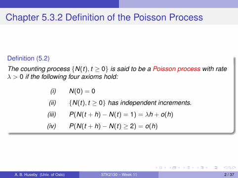
Definition (5.2)
The counting process {N(t), t ≥ 0} is said to be a Poisson process with rateλ > 0 if the following four axioms hold:
(i) N(0) = 0
(ii) {N(t), t ≥ 0} has independent increments.
(iii) P(N(t + h)− N(t) = 1) = λh + o(h)
(iv) P(N(t + h)− N(t) ≥ 2) = o(h)
A. B. Huseby (Univ. of Oslo) STK2130 – Week 11 2 / 37
Properties of the Poisson Process
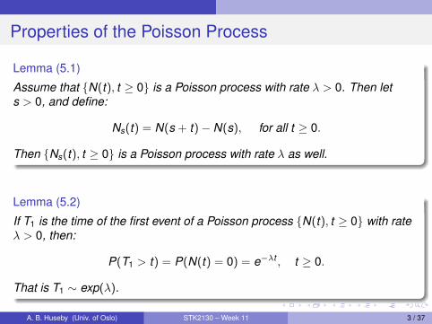
Lemma (5.1)
Assume that {N(t), t ≥ 0} is a Poisson process with rate λ > 0. Then lets > 0, and define:
Ns(t) = N(s + t)− N(s), for all t ≥ 0.
Then {Ns(t), t ≥ 0} is a Poisson process with rate λ as well.
Lemma (5.2)
If T1 is the time of the first event of a Poisson process {N(t), t ≥ 0} with rateλ > 0, then:
P(T1 > t) = P(N(t) = 0) = e−λt , t ≥ 0.
That is T1 ∼ exp(λ).
A. B. Huseby (Univ. of Oslo) STK2130 – Week 11 3 / 37
Properties of the Poisson Process (cont.)
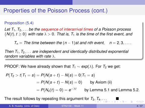
Proposition (5.4)
Let T1,T2, . . . be the sequence of interarrival times of a Poisson process{N(t), t ≥ 0} with rate λ > 0. That is, T1 is the time of the first event, and
Tn = The time between the (n − 1)st and nth event, n = 2,3, . . . .
Then T1,T2, . . . are independent and identically distributed exponentialrandom variables with rate λ.
PROOF: We have already shown that T1 ∼ exp(λ). For T2 we get:
P(T2 > t |T1 = s) = P(N(s + t)− N(s) = 0|T1 = s)
= P(N(s + t)− N(s) = 0) by Axiom (ii)
= P(Ns(t) = 0) = e−λt by Lemma 5.1 and Lemma 5.2.
The result follows by repeating this argument for T3,T4, . . . �
A. B. Huseby (Univ. of Oslo) STK2130 – Week 11 4 / 37
Properties of the Poisson Process (cont.)
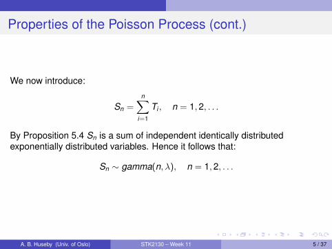
We now introduce:
Sn =n∑
i=1
Ti , n = 1,2, . . .
By Proposition 5.4 Sn is a sum of independent identically distributedexponentially distributed variables. Hence it follows that:
Sn ∼ gamma(n, λ), n = 1,2, . . .
A. B. Huseby (Univ. of Oslo) STK2130 – Week 11 5 / 37
Properties of the Poisson Process (cont.)
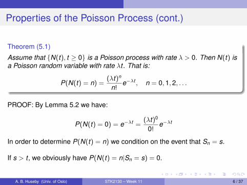
Theorem (5.1)
Assume that {N(t), t ≥ 0} is a Poisson process with rate λ > 0. Then N(t) isa Poisson random variable with rate λt . That is:
P(N(t) = n) =(λt)n
n!e−λt , n = 0,1,2, . . .
PROOF: By Lemma 5.2 we have:
P(N(t) = 0) = e−λt =(λt)0
0!e−λt
In order to determine P(N(t) = n) we condition on the event that Sn = s.
If s > t , we obviously have P(N(t) = n|Sn = s) = 0.
A. B. Huseby (Univ. of Oslo) STK2130 – Week 11 6 / 37
Properties of the Poisson Process (cont.)
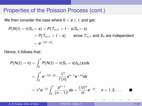
We then consider the case where 0 < s ≤ t , and get:
P(N(t) = n|Sn = s) = P(Tn+1 > t − s|Sn = s)
= P(Tn+1 > t − s) since Tn+1 and Sn are independent
= e−λ(t−s).
Hence, it follows that:
P(N(t) = n) =
∫ t
0P(N(t) = n|Sn = s)fSn (s)ds
=
∫ t
0e−λ(t−s) · λ
n
Γ(n)sn−1e−λsds
= λne−λt∫ t
0
sn−1
(n − 1)!ds =
(λt)n
n!e−λt , n = 1,2, . . . �
A. B. Huseby (Univ. of Oslo) STK2130 – Week 11 7 / 37
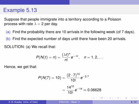
Example 5.13
Suppose that people immigrate into a territory according to a Poissonprocess with rate λ = 2 per day.
(a) Find the probability there are 10 arrivals in the following week (of 7 days).
(b) Find the expected number of days until there have been 20 arrivals.
SOLUTION: (a) We recall that:
P(N(t) = n) =(λt)n
n!e−λt , n = 1,2, . . .
Hence, we get that:
P(N(7) = 10) =(2 · 7)10
10!e−2·7
=1410
10!e−14 ≈ 0.06628
A. B. Huseby (Univ. of Oslo) STK2130 – Week 11 8 / 37
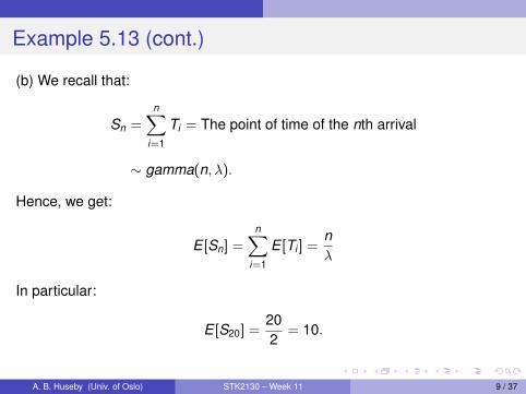
Example 5.13 (cont.)
(b) We recall that:
Sn =n∑
i=1
Ti = The point of time of the nth arrival
∼ gamma(n, λ).
Hence, we get:
E [Sn] =n∑
i=1
E [Ti ] =nλ
In particular:
E [S20] =202
= 10.
A. B. Huseby (Univ. of Oslo) STK2130 – Week 11 9 / 37
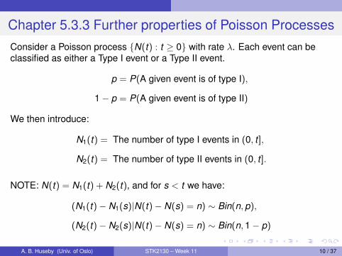
Chapter 5.3.3 Further properties of Poisson ProcessesConsider a Poisson process {N(t) : t ≥ 0} with rate λ. Each event can beclassified as either a Type I event or a Type II event.
p = P(A given event is of type I),
1− p = P(A given event is of type II)
We then introduce:
N1(t) = The number of type I events in (0, t ],
N2(t) = The number of type II events in (0, t ].
NOTE: N(t) = N1(t) + N2(t), and for s < t we have:
(N1(t)− N1(s)|N(t)− N(s) = n) ∼ Bin(n,p),
(N2(t)− N2(s)|N(t)− N(s) = n) ∼ Bin(n,1− p)
A. B. Huseby (Univ. of Oslo) STK2130 – Week 11 10 / 37
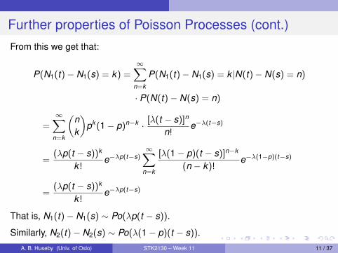
Further properties of Poisson Processes (cont.)From this we get that:
P(N1(t)− N1(s) = k) =∞∑
n=k
P(N1(t)− N1(s) = k |N(t)− N(s) = n)
· P(N(t)− N(s) = n)
=∞∑
n=k
(nk
)pk (1− p)n−k · [λ(t − s)]n
n!e−λ(t−s)
=(λp(t − s))k
k !e−λp(t−s)
∞∑n=k
[λ(1− p)(t − s)]n−k
(n − k)!e−λ(1−p)(t−s)
=(λp(t − s))k
k !e−λp(t−s)
That is, N1(t)− N1(s) ∼ Po(λp(t − s)).
Similarly, N2(t)− N2(s) ∼ Po(λ(1− p)(t − s)).A. B. Huseby (Univ. of Oslo) STK2130 – Week 11 11 / 37
Further properties of Poisson Processes (cont.)
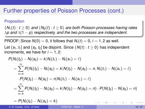
Proposition
{N1(t) : t ≥ 0} and {N2(t) : t ≥ 0} are both Poisson processes having ratesλp and λ(1− p) respectively, and the two processes are independent.
PROOF: Since N(0) = 0, it follows that Ni (t) = 0, i = 1,2 as well.
Let (s1, t1] and (s2, t2] be disjoint. Since {N(t) : t ≥ 0} has independentincrements, we have for i = 1,2:
P(Ni (t2)− Ni (s2) = k |Ni (t1)− Ni (s1) = `)
=∞∑
n=k
P(Ni (t2)− Ni (s2) = k |N(t2)− N(s2) = n,Ni (t1)− Ni (s1) = `)
· P(N(t2)− N(s2) = n|Ni (t1)− Ni (s1) = `)
=∞∑
n=k
P(Ni (t2)− Ni (s2) = k |N(t2)− N(s2) = n) · P(N(t2)− N(s2) = n)
= P(Ni (t2)− Ni (s2) = k)
A. B. Huseby (Univ. of Oslo) STK2130 – Week 11 12 / 37
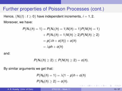
Further properties of Poisson Processes (cont.)Hence, {Ni (t) : t ≥ 0} have independent increments, i = 1,2.
Moreover, we have:
P(N1(h) = 1) = P(N1(h) = 1|N(h) = 1)P(N(h) = 1)
+ P(N1(h) = 1|N(h) ≥ 2)P(N(h) ≥ 2)
= p(λh + o(h)) + o(h)
= λph + o(h)
and:
P(N1(h) ≥ 2) ≤ P(N(h) ≥ 2) = o(h).
By similar arguments we get that:
P(N2(h) = 1) = λ(1− p)h + o(h)
P(N2(h) ≥ 2) = o(h).
A. B. Huseby (Univ. of Oslo) STK2130 – Week 11 13 / 37
Further properties of Poisson Processes (cont.)
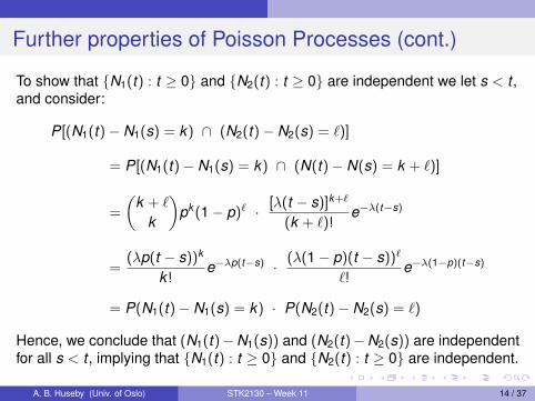
To show that {N1(t) : t ≥ 0} and {N2(t) : t ≥ 0} are independent we let s < t ,and consider:
P[(N1(t)− N1(s) = k) ∩ (N2(t)− N2(s) = `)]
= P[(N1(t)− N1(s) = k) ∩ (N(t)− N(s) = k + `)]
=
(k + `
k
)pk (1− p)` · [λ(t − s)]k+`
(k + `)!e−λ(t−s)
=(λp(t − s))k
k !e−λp(t−s) · (λ(1− p)(t − s))`
`!e−λ(1−p)(t−s)
= P(N1(t)− N1(s) = k) · P(N2(t)− N2(s) = `)
Hence, we conclude that (N1(t)−N1(s)) and (N2(t)−N2(s)) are independentfor all s < t , implying that {N1(t) : t ≥ 0} and {N2(t) : t ≥ 0} are independent.
A. B. Huseby (Univ. of Oslo) STK2130 – Week 11 14 / 37

Example 5.14
If immigrants to area A arrive at a Poisson rate of λ = 10 per week, and ifeach immigrant is of English descent with probability p = 1
12 . What is theprobability that no people of English descent will emigrate to area A duringthe month of February?
SOLUTION: By the previous proposition it follows that the number ofEnglishmen emigrating to area A during the month of February is Poissondistributed with mean:
λ · number of weeks in February · p = 10 · 4 · 112 = 10
3 .
Hence, we get:
P(no people of English descent in February)
=(10/3)0
0!e−10/3 = 0.0357
A. B. Huseby (Univ. of Oslo) STK2130 – Week 11 15 / 37

Example 5.15
We consider a Poisson process {N(t) : t ≥ 0} with rate λ where each eventrepresents an offer. We introduce:
Xi = The size of the i th offer , , i = 1,2, . . .
We assume that X1,X2, . . . are non-negative, independent and identicallydistributed random variables with density f (x). We assume that f (x) > 0 forall x ≥ 0 and introduce:
F̄ (x) = P(Xi > x), x ≥ 0.
POLICY: Accept the first offer greater than some chosen number y , anddefine:
Ny (t) = The number of offers greater than y in (0, t ], t ≥ 0.
Then {Ny (t) : t ≥ 0} is a Poisson process with rate λF̄ (y).
A. B. Huseby (Univ. of Oslo) STK2130 – Week 11 16 / 37
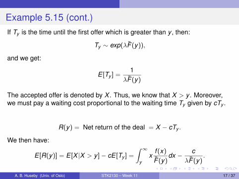
Example 5.15 (cont.)If Ty is the time until the first offer which is greater than y , then:
Ty ∼ exp(λF̄ (y)),
and we get:
E [Ty ] =1
λF̄ (y)
The accepted offer is denoted by X . Thus, we know that X > y . Moreover,we must pay a waiting cost proportional to the waiting time Ty given by cTy .
R(y) = Net return of the deal = X − cTy .
We then have:
E [R(y)] = E [X |X > y ]− cE [Ty ] =
∫ ∞y
xf (x)
F̄ (y)dx − c
λF̄ (y).
A. B. Huseby (Univ. of Oslo) STK2130 – Week 11 17 / 37
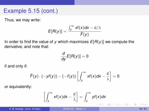
Example 5.15 (cont.)Thus, we may write:
E [R(y)] =
∫∞y xf (x)dx − c/λ
F̄ (y)
In order to find the value of y which maximizes E [R(y)] we compute thederivative, and note that:
ddy
E [R(y)] = 0
if and only if:
F̄ (y) · (−yf (y))− (−f (y))
[∫ ∞y
xf (x)dx − cλ
]= 0
or equivalently: [∫ ∞y
xf (x)dx − cλ
]=
∫ ∞y
yf (x)dx
A. B. Huseby (Univ. of Oslo) STK2130 – Week 11 18 / 37
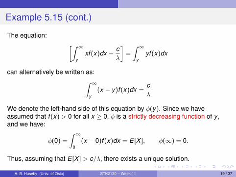
Example 5.15 (cont.)
The equation: [∫ ∞y
xf (x)dx − cλ
]=
∫ ∞y
yf (x)dx
can alternatively be written as:∫ ∞y
(x − y)f (x)dx =cλ
We denote the left-hand side of this equation by φ(y). Since we haveassumed that f (x) > 0 for all x ≥ 0, φ is a strictly decreasing function of y ,and we have:
φ(0) =
∫ ∞0
(x − 0)f (x)dx = E [X ], φ(∞) = 0.
Thus, assuming that E [X ] > c/λ, there exists a unique solution.
A. B. Huseby (Univ. of Oslo) STK2130 – Week 11 19 / 37
Example 5.15 (cont.)
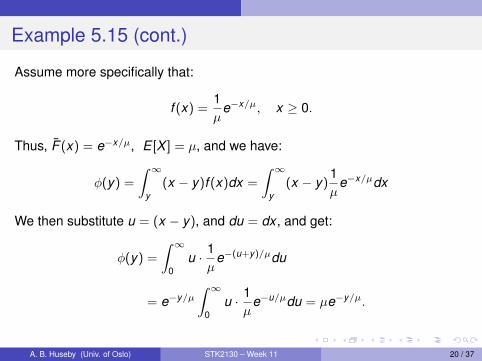
Assume more specifically that:
f (x) =1µ
e−x/µ, x ≥ 0.
Thus, F̄ (x) = e−x/µ, E [X ] = µ, and we have:
φ(y) =
∫ ∞y
(x − y)f (x)dx =
∫ ∞y
(x − y)1µ
e−x/µdx
We then substitute u = (x − y), and du = dx , and get:
φ(y) =
∫ ∞0
u · 1µ
e−(u+y)/µdu
= e−y/µ∫ ∞
0u · 1
µe−u/µdu = µe−y/µ.
A. B. Huseby (Univ. of Oslo) STK2130 – Week 11 20 / 37
Example 5.15 (cont.)
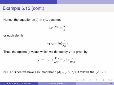
Hence, the equation φ(y) = c/λ becomes:
µe−y/µ =cλ
or equivalently:
−y/µ = ln(cλµ
)
Thus, the optimal y -value, which we denote by y∗ is given by:
y∗ = −µ ln(cλµ
) = µ ln(µ
c/λ)
NOTE: Since we have assumed that E [X ] = µ > c/λ it follows that y∗ > 0.
A. B. Huseby (Univ. of Oslo) STK2130 – Week 11 21 / 37
Example 5.15 (cont.)
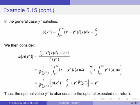
In the general case y∗ satisfies:
φ(y∗) =
∫ ∞y∗
(x − y∗)f (x)dx =cλ
We then consider:
E [R(y∗)] =
∫∞y∗ xf (x)dx − c/λ
F̄ (y∗)
=1
F̄ (y∗)
[∫ ∞y∗
(x − y∗)f (x)dx − cλ
+
∫ ∞y∗
y∗f (x)dx]
=1
F̄ (y∗)
[φ(y∗)− c
λ+ y∗F̄ (y∗)
]= y∗
Thus, the optimal value y∗ is also equal to the optimal expected net return.
A. B. Huseby (Univ. of Oslo) STK2130 – Week 11 22 / 37
Order statistics
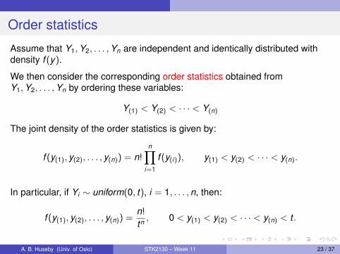
Assume that Y1,Y2, . . . ,Yn are independent and identically distributed withdensity f (y).
We then consider the corresponding order statistics obtained fromY1,Y2, . . . ,Yn by ordering these variables:
Y(1) < Y(2) < · · · < Y(n)
The joint density of the order statistics is given by:
f (y(1), y(2), . . . , y(n)) = n!n∏
i=1
f (y(i)), y(1) < y(2) < · · · < y(n).
In particular, if Yi ∼ uniform(0, t), i = 1, . . . ,n, then:
f (y(1), y(2), . . . , y(n)) =n!
tn , 0 < y(1) < y(2) < · · · < y(n) < t .
A. B. Huseby (Univ. of Oslo) STK2130 – Week 11 23 / 37
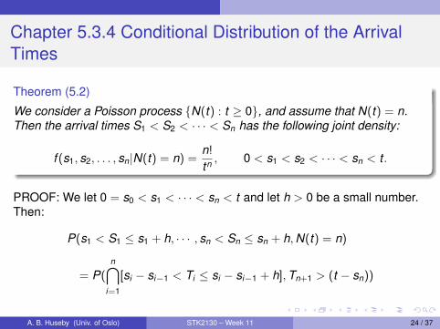
Chapter 5.3.4 Conditional Distribution of the ArrivalTimes
Theorem (5.2)
We consider a Poisson process {N(t) : t ≥ 0}, and assume that N(t) = n.Then the arrival times S1 < S2 < · · · < Sn has the following joint density:
f (s1, s2, . . . , sn|N(t) = n) =n!
tn , 0 < s1 < s2 < · · · < sn < t .
PROOF: We let 0 = s0 < s1 < · · · < sn < t and let h > 0 be a small number.Then:
P(s1 < S1 ≤ s1 + h, · · · , sn < Sn ≤ sn + h,N(t) = n)
= P(n⋂
i=1
[si − si−1 < Ti ≤ si − si−1 + h],Tn+1 > (t − sn))
A. B. Huseby (Univ. of Oslo) STK2130 – Week 11 24 / 37
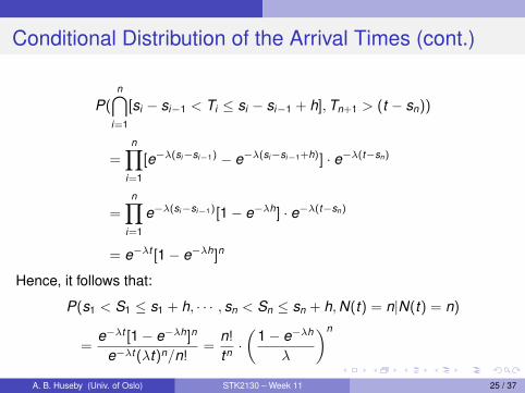
Conditional Distribution of the Arrival Times (cont.)
P(n⋂
i=1
[si − si−1 < Ti ≤ si − si−1 + h],Tn+1 > (t − sn))
=n∏
i=1
[e−λ(si−si−1) − e−λ(si−si−1+h)] · e−λ(t−sn)
=n∏
i=1
e−λ(si−si−1)[1− e−λh] · e−λ(t−sn)
= e−λt [1− e−λh]n
Hence, it follows that:
P(s1 < S1 ≤ s1 + h, · · · , sn < Sn ≤ sn + h,N(t) = n|N(t) = n)
=e−λt [1− e−λh]n
e−λt (λt)n/n!=
n!
tn ·(
1− e−λh
λ
)n
A. B. Huseby (Univ. of Oslo) STK2130 – Week 11 25 / 37
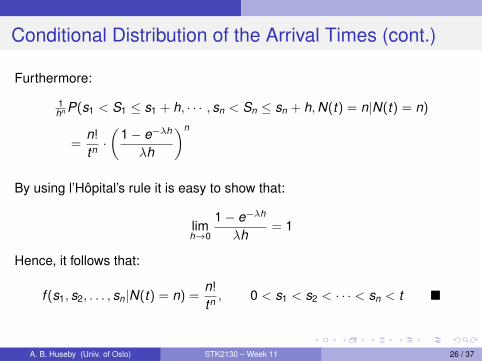
Conditional Distribution of the Arrival Times (cont.)
Furthermore:
1hn P(s1 < S1 ≤ s1 + h, · · · , sn < Sn ≤ sn + h,N(t) = n|N(t) = n)
=n!
tn ·(
1− e−λh
λh
)n
By using l’Hôpital’s rule it is easy to show that:
limh→0
1− e−λh
λh= 1
Hence, it follows that:
f (s1, s2, . . . , sn|N(t) = n) =n!
tn , 0 < s1 < s2 < · · · < sn < t �
A. B. Huseby (Univ. of Oslo) STK2130 – Week 11 26 / 37
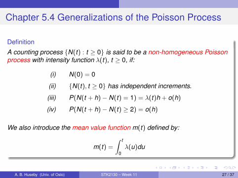
Chapter 5.4 Generalizations of the Poisson Process
Definition
A counting process {N(t) : t ≥ 0} is said to be a non-homogeneous Poissonprocess with intensity function λ(t), t ≥ 0, if:
(i) N(0) = 0
(ii) {N(t), t ≥ 0} has independent increments.
(iii) P(N(t + h)− N(t) = 1) = λ(t)h + o(h)
(iv) P(N(t + h)− N(t) ≥ 2) = o(h)
We also introduce the mean value function m(t) defined by:
m(t) =
∫ t
0λ(u)du
A. B. Huseby (Univ. of Oslo) STK2130 – Week 11 27 / 37
The non-homogeneous Poisson Process (cont.)
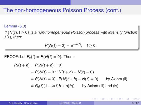
Lemma (5.3)
If {N(t), t ≥ 0} is a non-homogeneous Poisson process with intensity functionλ(t), then:
P(N(t) = 0) = e−m(t), t ≥ 0.
PROOF: Let P0(t) = P(N(t) = 0). Then:
P0(t + h) = P(N(t + h) = 0)
= P(N(t) = 0 ∩ N(t + h)− N(t) = 0)
= P(N(t) = 0) · P(N(t + h)− N(t) = 0) by Axiom (ii)
= P0(t)(1− λ(t)h + o(h)) by Axiom (iii) and (iv)
A. B. Huseby (Univ. of Oslo) STK2130 – Week 11 28 / 37
The non-homogeneous Poisson Process (cont.)
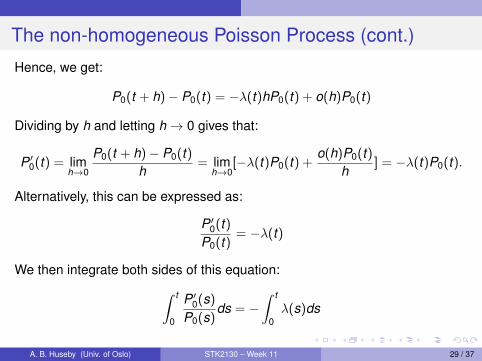
Hence, we get:
P0(t + h)− P0(t) = −λ(t)hP0(t) + o(h)P0(t)
Dividing by h and letting h→ 0 gives that:
P ′0(t) = limh→0
P0(t + h)− P0(t)h
= limh→0
[−λ(t)P0(t) +o(h)P0(t)
h] = −λ(t)P0(t).
Alternatively, this can be expressed as:
P ′0(t)P0(t)
= −λ(t)
We then integrate both sides of this equation:∫ t
0
P ′0(s)
P0(s)ds = −
∫ t
0λ(s)ds
A. B. Huseby (Univ. of Oslo) STK2130 – Week 11 29 / 37

The non-homogeneous Poisson Process (cont.)
On the left-hand side we substitute u = P0(s) and du = P ′0(s)ds, and get:∫ P0(t)
P0(0)
duu
= −∫ t
0λ(s)ds
The integration yields that:
log(P0(t))− log(P0(0)) = −∫ t
0λ(s)ds
Since P0(0) = P(N(0) = 0) = 1 it follows that:
P0(t) = e−∫ t
0 λ(s)ds = e−m(t), �
A. B. Huseby (Univ. of Oslo) STK2130 – Week 11 30 / 37
The non-homogeneous Poisson Process (cont.)
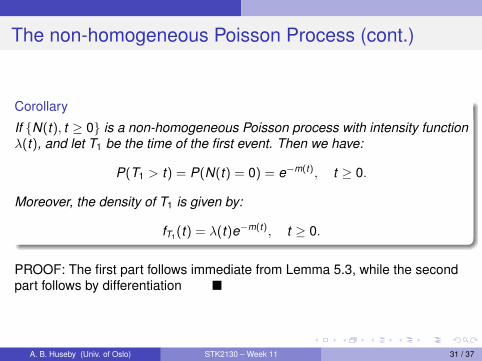
Corollary
If {N(t), t ≥ 0} is a non-homogeneous Poisson process with intensity functionλ(t), and let T1 be the time of the first event. Then we have:
P(T1 > t) = P(N(t) = 0) = e−m(t), t ≥ 0.
Moreover, the density of T1 is given by:
fT1 (t) = λ(t)e−m(t), t ≥ 0.
PROOF: The first part follows immediate from Lemma 5.3, while the secondpart follows by differentiation �
A. B. Huseby (Univ. of Oslo) STK2130 – Week 11 31 / 37
The non-homogeneous Poisson Process (cont.)
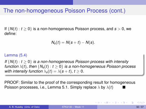
If {N(t) : t ≥ 0} is a non-homogeneous Poisson process, and s > 0, wedefine:
Ns(t) = N(s + t)− N(s).
Lemma (5.4)
If {N(t) : t ≥ 0} is a non-homogeneous Poisson process with intensityfunction λ(t), then {Ns(t) : t ≥ 0} is a non-homogeneous Poisson processwith intensity function λs(t) = λ(s + t), t ≥ 0.
PROOF: Similar to the proof of the corresponding result for homogeneousPoisson processes, i.e., Lemma 5.1. Simply replace λ by λ(t) �
A. B. Huseby (Univ. of Oslo) STK2130 – Week 11 32 / 37
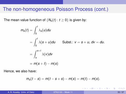
The non-homogeneous Poisson Process (cont.)
The mean value function of {Ns(t) : t ≥ 0} is given by:
ms(t) =
∫ t
0λs(u)du
=
∫ t
0λ(s + u)du Subst.: v = s + u, dv = du.
=
∫ s+t
sλ(v)dv
= m(s + t)−m(s)
Hence, we also have:
ms(t − s) = m(t − s + s)−m(s) = m(t)−m(s).
A. B. Huseby (Univ. of Oslo) STK2130 – Week 11 33 / 37
The non-homogeneous Poisson Process (cont.)
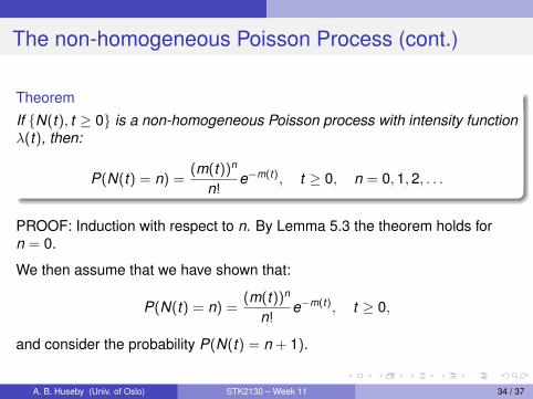
Theorem
If {N(t), t ≥ 0} is a non-homogeneous Poisson process with intensity functionλ(t), then:
P(N(t) = n) =(m(t))n
n!e−m(t), t ≥ 0, n = 0,1,2, . . .
PROOF: Induction with respect to n. By Lemma 5.3 the theorem holds forn = 0.
We then assume that we have shown that:
P(N(t) = n) =(m(t))n
n!e−m(t), t ≥ 0,
and consider the probability P(N(t) = n + 1).
A. B. Huseby (Univ. of Oslo) STK2130 – Week 11 34 / 37
The non-homogeneous Poisson Process (cont.)
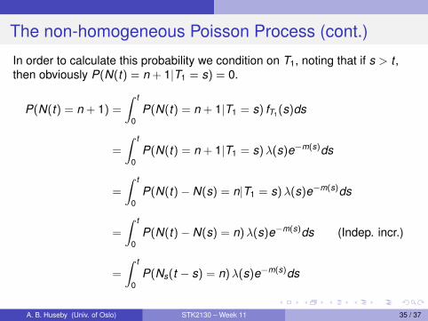
In order to calculate this probability we condition on T1, noting that if s > t ,then obviously P(N(t) = n + 1|T1 = s) = 0.
P(N(t) = n + 1) =
∫ t
0P(N(t) = n + 1|T1 = s) fT1 (s)ds
=
∫ t
0P(N(t) = n + 1|T1 = s)λ(s)e−m(s)ds
=
∫ t
0P(N(t)− N(s) = n|T1 = s)λ(s)e−m(s)ds
=
∫ t
0P(N(t)− N(s) = n)λ(s)e−m(s)ds (Indep. incr.)
=
∫ t
0P(Ns(t − s) = n)λ(s)e−m(s)ds
A. B. Huseby (Univ. of Oslo) STK2130 – Week 11 35 / 37
The non-homogeneous Poisson Process (cont.)
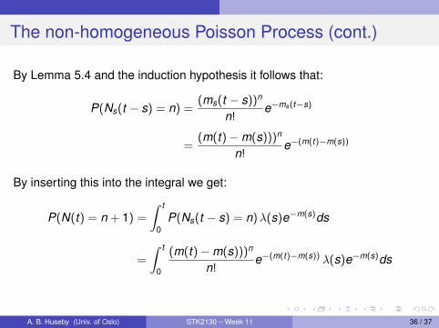
By Lemma 5.4 and the induction hypothesis it follows that:
P(Ns(t − s) = n) =(ms(t − s))n
n!e−ms(t−s)
=(m(t)−m(s)))n
n!e−(m(t)−m(s))
By inserting this into the integral we get:
P(N(t) = n + 1) =
∫ t
0P(Ns(t − s) = n)λ(s)e−m(s)ds
=
∫ t
0
(m(t)−m(s)))n
n!e−(m(t)−m(s)) λ(s)e−m(s)ds
A. B. Huseby (Univ. of Oslo) STK2130 – Week 11 36 / 37
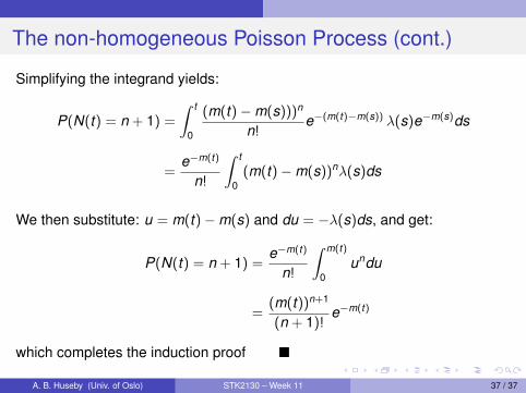
The non-homogeneous Poisson Process (cont.)
Simplifying the integrand yields:
P(N(t) = n + 1) =
∫ t
0
(m(t)−m(s)))n
n!e−(m(t)−m(s)) λ(s)e−m(s)ds
=e−m(t)
n!
∫ t
0(m(t)−m(s))nλ(s)ds
We then substitute: u = m(t)−m(s) and du = −λ(s)ds, and get:
P(N(t) = n + 1) =e−m(t)
n!
∫ m(t)
0undu
=(m(t))n+1
(n + 1)!e−m(t)
which completes the induction proof �
A. B. Huseby (Univ. of Oslo) STK2130 – Week 11 37 / 37