Embed Size (px)
Citation preview
UNIVERSITA DEGLI STUDI DI MILANO BICOCCA
Facolta di Scienze MM.FF.NN.
Dottorato di Ricerca in Informatica
XXII Ciclo
Stochastic algorithms forbiochemical processes
Paolo Cazzaniga
Supervisor Prof. Giancarlo Mauri
Tutor Prof. Paola Bonizzoni
PhD Coordinator Prof. Stefania Bandini
ANNO ACCADEMICO 2008–2009


iii
Acknowledgments
I would like to express my sincere gratitude to Professor Giancarlo Mauriwho has been my supervisor. He gave me many helpful suggestions andimportant advice during the course of my PhD.
Special thanks are due to Daniela Besozzi for her constant encourage-ment, her useful help (on many occasions) and her friendship.
I would also like to thank Dario Pescini for his assistance with writingcode, his great effort to explain things and for all the last minute rushes toairports and train stations because we were always late.
A particular thanks to Prof. Stephen Gilmore and Jane Hillston whohosted me for 6 months in Edinburgh. And I should also say thank you tomy flatmates, the guys working at the LFCS and all the other people I metthere.
I wish to thank the people working at DISCo for their friendship, helpand for the parties we had.
I am grateful to the people who helped me during my PhD, and to myfriends for the fun and laughter we shared.
Indeed, I owe a special thanks to my family for its support during thisperiod and to Laura who believed in me and supported me throughout myPhD.

Contents
Introduction ix
1 Stochastic algorithms for the simulation of biochemical sys-tems 1
1.1 Gillespie’s stochastic simulation algorithm . . . . . . . . . . . 2
1.2 The next reaction method . . . . . . . . . . . . . . . . . . . . 6
1.3 The tau-leaping algorithm . . . . . . . . . . . . . . . . . . . . 11
1.4 The next subvolume method . . . . . . . . . . . . . . . . . . 16
1.5 The binomial tau-leap spatial stochastic simulation algorithm 20
1.6 Other algorithms . . . . . . . . . . . . . . . . . . . . . . . . . 25
2 Optimization algorithms 29
2.1 Genetic algorithms . . . . . . . . . . . . . . . . . . . . . . . . 30
2.2 Particle swarm optimizer . . . . . . . . . . . . . . . . . . . . . 37
3 Membrane systems 45
3.1 Basic notions of membrane systems . . . . . . . . . . . . . . . 46
3.2 Dynamical probabilistic P systems . . . . . . . . . . . . . . . 52
3.3 A DPP application: metapopulation systems . . . . . . . . . 58
3.3.1 The modelling framework . . . . . . . . . . . . . . . . 60
3.3.2 Simulations and results . . . . . . . . . . . . . . . . . 66
3.3.3 Discussion . . . . . . . . . . . . . . . . . . . . . . . . . 72
4 τ–DPP 75
4.1 Tau-leaping procedure in DPPs . . . . . . . . . . . . . . . . . 76
4.2 τ -DPP algorithm . . . . . . . . . . . . . . . . . . . . . . . . . 80
4.3 A test case for τ -DPP . . . . . . . . . . . . . . . . . . . . . . 84
4.4 τ -DPP with size associated to volumes and objects . . . . . . 84
4.5 A test case for Sτ -DPP . . . . . . . . . . . . . . . . . . . . . 90
4.6 Implementation of the algorithms . . . . . . . . . . . . . . . . 94
4.7 Discussion and future developments . . . . . . . . . . . . . . 96
v
Contents
5 Modelling chemical and biological systems 995.1 The Ras/cAMP/PKA signalling pathway in the yeast Sac-
charomyces cerevisiae . . . . . . . . . . . . . . . . . . . . . . 101
5.1.1 The Ras/cAMP/PKA pathway description . . . . . . 1015.1.2 The stochastic model . . . . . . . . . . . . . . . . . . . 103
5.1.3 The Ras2 • GTP generation module . . . . . . . . . . 1065.1.4 Generation of cAMP, coupling with PKA and feed-
back loops . . . . . . . . . . . . . . . . . . . . . . . . . 107
5.1.5 Discussion . . . . . . . . . . . . . . . . . . . . . . . . . 1105.2 The repressilator: a genetic oscillators coupled with a quorum
sensing mechanism . . . . . . . . . . . . . . . . . . . . . . . . 113
5.2.1 A multivolume model for coupled genetic oscillators . 1145.2.2 Results of simulations . . . . . . . . . . . . . . . . . . 116
5.2.3 Discussion and future developments . . . . . . . . . . 1215.3 First steps toward a wet implementation for τ -DPP . . . . . 122
5.3.1 Chemical computing . . . . . . . . . . . . . . . . . . . 1235.3.2 Definition and simulation of component reaction net-
works using τ -DPP . . . . . . . . . . . . . . . . . . . . 125
5.3.2.1 The NAND and XOR logic circuits . . . . . 1265.3.2.2 Fredkin gates and circuits . . . . . . . . . . . 130
5.3.2.3 The SUB instruction . . . . . . . . . . . . . 1385.3.2.4 The SUBADD module . . . . . . . . . . . . . 140
5.3.3 Discussion and open problems . . . . . . . . . . . . . . 141
5.4 A study on the combined interplay between stochastic fluc-tuations and the number of flagella in bacterial chemotaxis . 144
5.4.1 The modeling of bacterial chemotaxis . . . . . . . . . 145
5.4.2 Stochastic simulations of chemotactic response regulator1495.4.3 The interplay between stochastic fluctuations and the
number of bacterial flagella . . . . . . . . . . . . . . . 153
5.4.4 Discussion . . . . . . . . . . . . . . . . . . . . . . . . . 157
6 The role of parameters in chemical and biological systems 161
6.1 Parameter estimation of biochemical systems . . . . . . . . . 163
6.2 Parameter sweep application . . . . . . . . . . . . . . . . . . 1656.3 Fitness function . . . . . . . . . . . . . . . . . . . . . . . . . . 166
6.4 A comparison of GAs and PSO for parameter estimation instochastic biochemical systems . . . . . . . . . . . . . . . . . 1696.4.1 Systems of biochemical reactions . . . . . . . . . . . . 169
6.4.2 GAs and PSO settings . . . . . . . . . . . . . . . . . . 1716.4.3 Experimental results . . . . . . . . . . . . . . . . . . . 172
6.4.4 Discussion . . . . . . . . . . . . . . . . . . . . . . . . . 1766.5 Stochastic simulations on a grid framework
for parameter sweep applications in biological models . . . . . 178
6.5.1 The EGEE grid platform . . . . . . . . . . . . . . . . 179
vi

Contents
6.5.2 PSA over the grid . . . . . . . . . . . . . . . . . . . . 1806.5.3 Bacterial chemotaxis: a case study . . . . . . . . . . . 1836.5.4 Results . . . . . . . . . . . . . . . . . . . . . . . . . . 1846.5.5 Performance discussion . . . . . . . . . . . . . . . . . 1876.5.6 Conclusion . . . . . . . . . . . . . . . . . . . . . . . . 193
7 Conclusion and future work 195
Bibliography 201
vii

Introduction
Aims and motivations
After the completion of the human genome sequencing (and of a lot of othergenomes), the main challenge for the modern biology is to understand com-plex biological processes such as metabolic pathways, gene regulatory net-works and cell signalling pathways, which are the basis of the functioning ofliving cells. This goal can only be achieved by using mathematical modellingtools and computer simulation techniques, to integrate experimental dataand to make predictions on the system behaviour that will be then exper-imentally checked, so as to gain insights into the working and the generalprinciples of organization of biological systems.
In fact, the formal modelling of biological systems allows the develop-ment of simulators, which can be used to understand how the described sys-tem behaves in normal conditions, and how it reacts to (simulated) changesin the environment or to alterations of some of its components. Simulationspresent many advantages over conventional experimental biology in termsof cost, ease to use and speed. For instance, some experiments that areinfeasible in vivo can be conducted in silico, e.g. it is possible to knock outmany vital genes from the cells and monitor their individual and collectiveimpact on cellular metabolism. Evidently such experiments cannot be donein vivo because the cell may not survive. Therefore, the development of pre-dictive in silico models offers opportunities for unprecedented control overthe system.
In the last few years a wide variety of models of cellular processes havebeen proposed, based on different formalisms. For example, chemical kineticmodels attempt to represent a cellular process as a system of distinct chemi-cal reactions. In this case, the network state is defined by the instantaneousquantity (or concentration) of each molecular species of interest in the cell,and different molecular species may interact via one or more reactions. Usu-ally, reactions are represented by a system of coupled differential equationsthat relate the quantity of reactants to the quantity of products, accordingto a reaction rate and other parameters.
Recently, it has been pointed out that transcription, translation andother cellular processes may not behave deterministically but instead are
ix

Introduction: aims and motivations
better modelled as random events [123]. Several models address this concernby abandoning differential equations in favour of stochastic relations thatdescribe each chemical reaction in terms of molecular collisions [6, 74].
The use of stochastic methods for the study of biological systems ismotivated by the fact that these systems are usually composed by manychemical interactions among a large number of chemical species, wherebythe molecular quantities involved can be small (few tens of molecules). Insystems having these characteristics, noise plays a major role in the system’sdynamics [128].
Two different kind of noise can be identified in biological systems: ex-trinsic and intrinsic [59, 176]. The first one is related to the experimentalconditions; for instance, the variation of temperature, pressure, light, orfluctuations of other cellular factors, are all sources of extrinsic noise. Onthe other hand, there are stochastic events occurring during the processes ofgene expression, at the level of transcription, translation and protein degra-dation, which result in intrinsic noise.
The role of noise in biological systems has been studied and quantified[59, 176, 192], proving that the classic deterministic and continuous ap-proach (like, for instance, ordinary differential equations) is unsuitable forthe modelling, simulation and analysis of phenomena like cellular pathways,especially when the gene transcription and translation machinery is involved.
The deterministic approach is based on the law of mass action, an empir-ical law which provides a simple relation between reaction rates and molec-ular species concentrations. Given the initial molecular concentrations, byusing the law of mass action, a temporal description of the component con-centrations can be obtained. The law of mass action considers chemicalreactions to be macroscopic, continuous and deterministic. However, in thestudy of “small” systems, the law of mass action becomes inadequate, andit more is suitable to apply stochastic approaches, since (1) they take intoaccount the discreteness of the quantity of the molecular species and theinherently random character of the phenomena; (2) they are in accordancewith the theories of thermodynamics and stochastic processes; and (3) theyare appropriate for the description of systems characterised by instabilityphenomena [198].
On the other hand, one major problem related to stochastic methodsis that they are difficult to implement analytically; hence, they are im-plemented by means of numerical simulations whose computation time isusually very expensive.
In this thesis we provide a discrete and stochastic framework for themodelling, simulation and analysis of biological and chemical systems. Tothis aim, we will start from the description of other techniques and meth-ods that are present in literature, as the basis to build and compare ourapproach.
At a different level of abstraction many formalisms have been employed
x
to model biological systems. Some of these have been originally developedby computer scientists to model systems of interacting components, such asPetri Nets [165] or π-calculus [133], while others have been proposed for thestudy of biochemical systems, like κ-calculus [43] and Bio-PEPA [36]. More-over, formalisms such as membrane systems [154], originally proposed as amodel of computation inspired by biology, have recently found applicationto the formal description and modelling of biological phenomena.
Starting from the notion of membrane systems (or P systems), we providethe definition of one of their particular variant called dynamical probabilis-tic P systems (DPPs) [162]. P systems, and in particular DPPs, representan appropriate tool for the modelling of biochemical systems, they providea suitable structure (called membrane structure) which can be used to de-scribe the spatial arrangement of the compartments involved in a system.Moreover, inside each compartment, a set of chemical reactions written asmultiset rewriting rules can be specified, together with a set of molecularspecies specified as multisets of objects. The evolution of a system is ob-tained by means of the application of the rules on the objects currentlypresent inside the membranes. In the basic definition of P systems, therules are applied in a nondeterministic and maximally parallel manner, andat each step all the objects which can evolve should evolve. In DPPs, themaximal parallelism has been mitigated by assigning probabilities to therules, and these values vary according to the system state. By exploitingthese values, it is possible to provide a description of the system’s dynamics,that is, DPPs allow to reproduce the stochastic variations of the elements(i.e. chemical species) occurring in the system. However, this descriptionis only qualitative, in the sense that an effective (physical) time streamlinecannot be directly associated to the evolution steps of the system.
The temporal dynamics of a biochemical system composed by manyvolumes can be simulated by integrating a stochastic algorithm with theframework of DDPs. The stochastic simulation algorithm [74] representsthe seminal procedure used for reproducing the exact dynamics of a sys-tem that is enclosed in a single volume, which is assumed to be well stirred(i.e. homogeneous, in the sense that molecules are considered uniformlydistributed) and at constant temperature. One of the main drawbacks ofthis procedure is the computational time required to obtain the behaviourof a system, because this task is achieved by simulating one reaction perstep. More recently, several algorithms have been proposed in order to over-come this limitation; among others, in this thesis we recall the next reactionmethod [72] – a procedure that executes reactions in a sequential manner,but exploits suitable data structure to update the system’s state and to han-dle the additional information required during the simulation, thus speedingup the computation – and the tau-leaping algorithm [77], a method basedon a strategy that allows to select and execute in parallel several reactionsper step. Tau-leaping represents one of the most efficient algorithms for the
xi
Introduction: aims and motivations
description of the dynamics of biochemical systems. However, these algo-rithms share the same limitation: they are only applicable to homogeneoussystems enclosed in a single volume.
Nevertheless, many cellular processes are characterised by a spatial het-erogeneity [182], where diffusion plays an important role for the systemdynamics, e.g. the living cell. In order to describe the spatial heterogeneity,there exist methods that divide the reaction volume in a number of subvol-umes ,and then consider both reaction and diffusion processes to describethe behaviour of the entire system.
For instance, the next subvolume method [57] provides the dynamics of aheterogeneous system composed by many subvolumes, by sequentially sim-ulating a single reaction or diffusion event inside one subvolume selectedat the beginning of each iteration. The computation time required to exe-cute this procedure is usually high, hence, to speed up the computation thesame data structures used in the next reaction method are exploited hereto manage the information of the subvolumes. Another example of stochas-tic algorithm for the simulation of heterogeneous systems is the binomialtau-leap spatial stochastic simulation algorithm [117] which is based on thenext subvolume method, but exploits a particular version of the tau-leapingalgorithm to describe the dynamics of the subvolumes, resulting in a moreefficient simulation procedure (with respect to the next subvolume method).The main drawback of these two procedures concerns the high computationtime required to run a simulation, since both algorithms update the internalstate of a single subvolume during each iteration.
In order to overcome the limitations of DPPs and of the stochastic algo-rithms cited here, in this thesis we introduce a novel method for the mod-elling and simulation of biochemical systems, which combines the descriptivepower of DPPs with the efficiency of tau-leaping algorithm. This approach,called τ -DPP [30], exploits the membrane structure and the system defini-tion of DPPs, with the aim of describing multiple volume systems, and usesa modified version of the tau-leaping algorithm for the description of thesystem behaviour. Differently from DPPs, where the obtained dynamics isonly qualitative, with τ -DPP it is possible to provide the quantitative be-haviour, by assigning a time increment to each simulation step. In orderto investigate systems consisting of many volume, the tau-leaping algorithmhas been modified to handle the communication between volumes. The pro-posed strategy allows to synchronise volumes by computing a common timeincrement and using it to select the set of reactions to apply (at each step),inside every membrane, thus resulting in a parallel evolution of the entiresystem.
A different version of τ -DPP, called Sτ -DPP [29], is also presented. InSτ -DPP, we allow the communication between non-adjacent membranes,and we associate a measure to membranes and objects, representing the“size” of the volumes where the computation occurs and the volume of each
xii
object, respectively. Both the sizes of membranes and objects are useful todescribe any real system where it is important to avoid the infinite accumu-lation of objects inside a membrane, which is very important in chemical andbiological systems, and cannot be achieved by simply bounding the “capac-ity” of the membranes or by limiting the maximum number objects allowedinside a particular volume.
The frameworks presented in this thesis have been used for the mod-elling, simulation and analysis of ecological, biological and chemical sys-tems. In particular, we present an application of DPPs for the investigationof metapopulations, also called multi-patch systems, which are ecologicalmodels used to analyse the behaviour of interacting populations, to the aimof determining how a fragmented habitat influences local and global popu-lation persistence.
Then, the framework of τ -DPP has been applied to an extensive study ofdifferent biological systems. For instance, we present a discrete mathemat-ical model for the Ras/cAMP/PKA pathway in the yeast Saccharomycescerevisiae, which is involved in the regulation of metabolism and cell cycleprogression [31]. We investigate this system under various conditions, andwe test how different values of several stochastic reaction constants affectthe pathway behaviour.
A model of a genetic oscillator coupled with a quorum sensing inter-cellular mechanism is also considered as a case study [18]. This intercellu-lar communication mechanism is able to lead the local genetic oscillators,within a noisy and nonidentical population, to global oscillatory rhythms.In particular, it was shown that individual repressilator systems can self-synchronize, even when their periods are broadly distributed [67]. The mul-tivolume model of this system consists of n volumes, each one correspondingto a cell, enclosed inside an additional volume representing the environment.
Then, the modelling and stochastic simulations of the chemotactic sig-nal transduction pathway in bacteria, are presented [14]. This particularpathway allows bacteria to respond and adapt to environmental changes, bytuning their tumbling and running motions that are due to clockwise andcounterclockwise rotations of their flagella. By exploiting the model andthe results of simulations obtained with τ -DPP, we investigate the interplaybetween the stochastic fluctuations of the amount of a particular proteinof this pathway and the number of cellular flagella as the core componentthat stands at the basis of chemotactic motions. The aim of this analysisis to devise the mean time periods during which the cell either performs arunning or a tumbling motion, considering both the coordination of flagellaand the randomness that is intrinsic in the chemotactic pathway.
A simple biochemical system has been simulated by means of Sτ -DPP.The system describes the transport of molecules from the cytoplasm (mod-elled as a set of nested membranes) to the nucleus. This task can be accom-plished by using simple communication rules or by means of a microtubule
xiii
Introduction: aims and motivations
[167], which is a sort of intracellular “highway” that efficiently transportmolecules towards the nucleus. Here, by changing the size associated to themembranes representing the microtubule, we highlight the role played bythe “space” and its effects on the system’s dynamics.
We consider also a different issue, that is related to a possible implemen-tation of τ -DPP by means of chemical systems. To this aim, we introduce theframework of chemical computing, in order to show how to describe “com-putations” performed with τ -DPP, by means of chemical reactions [164].In particular, we present the encoding of simple boolean functions, of theFredkin gate and an instance of Fredkin circuit. The encoding of simplelogic gates is useful because by composing them in particular circuits, it ispossible to encode any boolean function. Besides this, we also present en-codings for register machines instructions, and we give some insights aboutthe construction of a complete register machine with n registers, with theaim to obtain a “parallel device” that can be used, for instance, in the fieldof computational complexity theory.
Another key issue related to the modelling of biochemical systems re-gards the calibration of the parameters. For instance, in the τ -DPP appli-cations presented in this thesis, the values of stochastic constants associatedto the chemical reaction have been obtained by first assuming plausible rel-ative magnitudes for their values, and then by adjusting them one by one,until a good reproduction of the expected behaviour has been obtained.
In general, many numerical factors are needed for a complete and accu-rate description of biological systems, like molecular species quantities andreaction rates, which represent an indispensable quantitative informationto perform computational investigations of the system behaviour. Unfortu-nately, the experimental values of these factors are often not available orinaccurate, since carrying out their measurements in vivo can be tanglingor even impossible [173]. In a few cases, the values of some parameters of agiven system can be estimated either from in vitro experiments (by fittingthe dynamics derived through equations based on mass-action law againstthe concentration time series that result from these measurements), or byassuming some analogies with similar processes or organisms for which moreexperimental data are available.
The lack and the inaccuracy of these information bring about the chal-lenging problem of developing suitable techniques to automatically estimatethe correct values to all parameters in order to reproduce the expected dy-namics in the best possible way.
Optimization methods can be used to tackle the calibration problem ofparameter estimation of biochemical systems by minimizing a cost func-tion (e.g. a distance measure) which quantitatively defines how good is thesystem behaviour, using the predicted values, with respect to the experi-mental dynamics. Several global optimization techniques have already beenadopted for parameter estimation of biochemical and biological systems.
xiv
In this thesis, we consider the application of two optimisation techniques,genetic algorithms and particle swarm optimizer, to tackle this problem.To this aim, we provide the definition of a fitness function that is suitableto quantify the quality of a particular set of parameters used during thestochastic simulation of a system. Working in the field of stochastic mod-elling and simulation, the fitness definition is based on the idea that we haveto compare the observed dynamics with the dynamics generated by using astochastic simulation algorithm, which will run using a particular set of pa-rameter values. Therefore, we have to manage some troublesome propertiesthat are inherent to stochastic simulations like, for instance, the irregulartime sampling of the resulting outcome.
In this thesis, in particular, we test and compare the performances ofgenetic algorithms and particle swarm optimization to the aim of identify themost suitable optimisation technique for the parameter estimation. To thisaim, these methods are applied to two simple biochemical schemes, whichhave been chosen since they are well representative of the dynamics of manyother biological systems: a basic catalytic kinetics (the Michaelis-Mentensystem) and an oscillating behaviour (based on the Belousov-Zhabotinskiireaction) [15]. The oscillating systems has been considered with two differentset of parameters which provide two distinct dynamics, characterised bysustained oscillations and a dynamics with damped oscillations, respectively.
Finally, the problem related to the exploration of the parameters space ofa biochemical system is described. Usually, this kind of analysis is achievedby means of large numbers of independent simulations where each execu-tion is performed with a particular parametrisation. To efficiently tacklethis problem, we present the implementation of a parameter sweep appli-cation on a grid framework [140], obtained by distributing large numbersof simulations performed by means of τ -DPP. This grid implementation isused in 4 different parameter sweep applications executed on a model ofthe chemotactic signal transduction pathway in bacteria composed by 59chemical reactions, and their performances are analysed and compared.
Overview
This thesis is structured as follows. In the first part (Chapters 1–3) weintroduce the prerequisite notions that are necessary for the development ofour work. In the second part (Chapter 4–6) we present our approach forthe modelling and simulation of biochemical systems, together with someapplications, as well as the tool for the analysis of the parameter space of asystem.
In Chapter 1, the main stochastic algorithms for the description of thedynamics of biochemical systems are presented. We start by introducingthe basic notions and the fundamental hypothesis needed for the develop-
xv
Introduction: aims and motivations
ment and the application of these algorithms. The reference procedure is thestochastic simulation algorithm (SSA), whose theoretical basis is exploited inmost of the other stochastic algorithms. Afterwards, we present (1) the nextreaction method, which is faster than SSA since it uses suitable data struc-ture to efficiently handle the computation and re-uses (previously drawn)random numbers; (2) the tau-leaping algorithm, an approximate procedurein which reactions are applied in parallel to achieve fast simulations; (3) thenext subvolume method ; (4) the Binomial tau leap spatial stochastic simula-tion algorithm for the simulation of heterogeneous systems composed by anumber of sub-volumes.
In Chapter 2, two optimisation techniques are presented: genetic algo-rithms and particle swarm optimizer. Genetic algorithms are a populationbased heuristic which select the individuals for the next generation accordingto their quality, and evolve them by means of variation operators. Particleswarm optimizer moves a swarm of particles through a n-dimensional space,towards the best position found so far by each particle and by the entireswarm. In the investigation of biochemical systems, both techniques can beapplied to tackle the parameter estimation issue, which consists in the cali-bration of the system’s parameters (this particular application is presentedin Chapter 6).
In Chapter 3, the framework of membrane systems, or P systems, isdescribed. First, the basic notions and definitions of P systems are pro-vided. Then, the variant of dynamical probabilistic P systems (DPP) isintroduced. DPPs propose a new approach for the application of P systems,which consists in interpreting them as stochastic tools for the descriptionof the dynamics of complex systems. The key feature is that, unlike thebasic version of P systems, in DPPs probabilities are associated with therules (following a method similar to that used in SSA), and these valuesvary during the evolution of the system according to a prescribed strategy.The “evolution” of a system described by DPPs is therefore governed by astochastic process. We present an application of DPPs for the modellingand simulation of a multivolume system, called metapopulations, which areecological models that describe the behaviour of interacting populations, tothe aim of determining how a fragmented habitat influences local and globalpopulation persistence.
In Chapter 4 we present a novel technique for the simulation of complexbiochemical systems, which combines the descriptive power of membranesystems with the efficiency of tau-leaping procedure. This method is calledτ -DPP, it represents an extension of the DPP variant of membrane sys-tems, since it introduces a strategy for providing quantitative descriptionsof a system’s dynamics. τ -DPP also extends the applicability of tau-leapingsimulation algorithm, as it provides a novel procedure to simulate systemsconsisting of many volumes, but still relying on the efficiency of the originalsimulation procedure. A further version of τ -DPP, called Sτ -DPP, is then
xvi
presented. It represents an improvement of the previous version since it con-siders the size of objects (molecules) and compartments (volumes) involvedin the system. In this case, the application of a set of rules is enabled onlyif the compartment where they are applied contains enough free space forthe freshly produced (or communicated) objects.
In Chapter 5 different applications of τ -DPP are provided. For each ap-plication, the model described by means of τ -DPP framework is presented,along with the results obtained by simulating the system. The first applica-tion regards the Ras/cAMP/PKA signalling pathway in the yeast Saccha-romyces cerevisiae, which is involved in the regulation of metabolism and cellcycle progression. The second application is a model of a genetic oscillatorcalled repressilator, coupled with a quorum sensing intercellular mechanism.The third application is related to a model of the chemotactic signal trans-duction pathway in bacteria. Finally, the implementation of boolean gates,circuits and register machine instructions, exploiting the chemical comput-ing theory, is also presented within the framework of τ -DPP.
In Chapter 6 we give a detailed description of the role played by theparameters of a biochemical system, focusing on the stochastic constantsassociated to the chemical reactions. We present the parameter estimationissue, that is, the problem related to the calibration of the system’s param-eters, and the parameter sweep application, a method suitable to explorethe space defined by the system’s parameters. In particular, we provide thedefinition of the fitness functions that we use both in parameter estimationto evaluate the quality of a particular set of parameters, and in the param-eter sweep to quantify the difference between the “wild type” dynamics andthose obtained by using different parametrisations. In particular, we presentan implementation of genetic algorithms and particle swarm optimizer totackle the parameter estimation issue, and we compare their performanceby applying them to simple biochemical networks. Then, we propose a gridimplementation of the parameter sweep application, obtained by distribut-ing a large number of simulations performed by means of τ -DPP, to the aimof efficiently exploring the parameter space of a biochemical system.
Finally, in Chapter 7 conclusive remarks and a discussion about the pre-sented work are proposed. Insights concerning some possible improvementsand future directions for research are also briefly described.
Published works
The work of this thesis is based on the following publications:
D. Besozzi, P. Cazzaniga, D. Pescini, G. Mauri. A multivolume approachto stochastic modelling with membrane systems. In: AlgorithmicBioprocesses, (A. Condon, D. Harel, J.N. Kok, A. Salomaa, E. Winfree,eds.), Natural Computing Series, Springer-Verlag, 519-542, 2009.
xvii
Introduction: aims and motivations
P. Cazzaniga, G. Mauri, L. Milanesi, E. Mosca, D. Pescini. A novel vari-ant of tissue P systems for the modelling of biochemical systems.Proceedings of the 10th International Workshop on Membrane Computing,WMC 2009 (G. Paun, M.J. Perez-Jimenez, A. Riscos-Nunez, G. Rozenberg,A. Salomaa, eds.), to appear in LNCS.
E. Mosca, P. Cazzaniga, D. Pescini, I. Merelli, G. Mauri, L. Milanesi.Stochastic simulations on a grid framework for parallel sweep ap-plications in biological models. Accepted for presentation at HiBi09 -High Performance Computational Systems Biology Workshop, 14-16 Octo-ber 2009 - Trento, Italy (submitted to Briefings in Bionformatics).
D. Besozzi, P. Cazzaniga, M. Dugo, D. Pescini, G. Mauri. A study on thecombined interplay between stochastic fluctuations and the num-ber of flagella in bacterial chemotaxis. Proceedings of CompMod2009- 2nd International Workshop on Computational Models for Cell Processes(R.J. Back, I. Petre, E. de Vink, eds.), EPTCS, 6, 47-62, 2009.
P. Cazzaniga, D. Pescini, L. Vanneschi, D. Besozzi, G. Mauri. A com-parison of genetic algorithms and particle swarm optimization forparameter estimation in stochastic biochemical systems. Proceed-ings of EvoBio 2009 (C. Pizzuti, M.D. Ritchie, M. Giacobini, eds.), LNCS5483, 116-127, 2009.
D. Pescini, P. Cazzaniga, C. Ferretti, G. Mauri. First steps toward awet implementation for tau-DPP. Proceedings of the 9th InternationalWorkshop on Membrane Computing, WMC 2008 (D. W. Corne, P. Frisco,G. Paun, G. Rozenberg, A. Salomaa, eds.), LNCS 5391, 355-373, 2009.
P. Cazzaniga, D. Pescini, D. Besozzi, G. Mauri, S. Colombo, E. Martegani.Modeling and stochastic simulation of the Ras/cAMP/PKA path-way in the yeast Saccharomyces cerevisiae evidences a key regu-latory function for intracellular guanine nucleotides pools. Journalof Biotechnology, 133, 3, 377-385, 2008.
D. Besozzi, P. Cazzaniga, D. Pescini, G. Mauri. Modelling metapopula-tions with stochastic membrane systems. BioSystems, 91, 3, 499-514,2008.
D. Besozzi, P. Cazzaniga, D. Pescini, G. Mauri. Seasonal variance in Psystem models for metapopulations. Progress in Natural Science, 17,4, 392-400, 2007.
P. Cazzaniga, D. Pescini, D. Besozzi, G. Mauri. Tau leaping stochas-tic simulation method in P systems. Proceedings of the 7th Interna-tional Workshop on Membrane Computing, WMC 2006 (H.J. Hoogeboom,G. Paun, G. Rozenberg, A. Salomaa, eds.), LNCS 4361, 298-313, 2006.
xviii
Chapter 1
Stochastic algorithms for thesimulation of biochemicalsystems
In this chapter, some of the most used and well known stochastic simulationtechniques will be presented. These techniques can be used to describethe dynamics of biochemical systems with fixed conditions (i.e. pressure,temperature, etc.), in which the set of molecular species involved, and thepossible interactions between species (chemical reactions) are known. Inparticular two exact procedures, the stochastic simulation algorithm [74] andthe next reaction method [72] will be presented. These two algorithms canbe applied to homogeneous systems, that is, systems in which the moleculesare considered well mixed, and they provide a sequential description of thesystem’s dynamics, by executing one reaction during each simulation step.The former is Gillespie’s seminal work, which represents the basis of mostof the stochastic algorithms for the simulation of chemical systems; thelatter has been introduced by Gibson and Bruck as a faster version of thestochastic simulation algorithm. The exactness of these two methods refersto the simulated evolution of the analysed system, which corresponds to an“exact” numerical realisation of the actual dynamics of the system.
An approximate simulation technique called tau-leaping, firstly presentedin [77], will be then described. This method has been developed in orderto speed up stochastic simulations, in fact, many reactions are executedduring each iteration. On the other hand, with this method there is a lossin the accuracy of the simulated dynamics with respect to the stochasticsimulation algorithm. In the following, we will refer in particular to thetau-leaping version presented in [26].
Finally, two stochastic algorithms used to simulate heterogeneous sys-tems will be illustrated. These procedures are called next subvolume method[57] and binomial tau-leap spatial stochastic simulation algorithm [117]. The-
1
Chapter 1. Stochastic algorithms for the simulation of biochemical systems
se procedures consider both reactive and diffusive processes, which occurinside the adjacent subvolumes constituting the analysed system. In par-ticular, the former method is based on the stochastic simulation algorithm,and simulates one event for each iteration step; the latter is based on thetau-leaping, hence many reaction and diffusive events are simulated duringeach step.
1.1 Gillespie’s stochastic simulation algorithm
In this section, the stochastic simulation algorithm (SSA) will be presented.This simulation technique has been introduced by Gillespie [73, 74] in orderto reproduce the exact behaviour of chemical systems. SSA represents thereference point for the development of new procedures, and it is one of themost used algorithms for the description of the dynamics of chemical andbiological systems. As a matter of fact, SSA has been implemented withinmany software tools [188, 41, 50, 33].
SSA can be applied to chemical systems defined within a single volumeΩ, which is assumed to be well stirred and at constant temperature. This isthe fundamental assumption that leads to the possibility of describing thesystem behaviour, without considering the position and velocity of every sin-gle molecule occurring inside the system. Inside Ω, a set of chemical speciesS1, . . . , SN, whose interactions are governed by a set of chemical reactionsR1, . . . , RM, is considered. A stochastic constant cj (j = 1, . . . ,M), whichdepends only on the chemical and physical properties of the molecules andon the temperature of the system, is associated to each reaction Rj . Thenumber of molecules of species Si (i = 1, . . . , N) at a given time t is de-noted by Xi(t), and the state of the system at time t is defined as the vectorX(t) ≡ (X1(t), . . . ,XN (t)).
It is clear that the changes in the molecular numbers of the species in-volved in the systems are a consequence of the application of the chemicalreactions. A chemical reaction Rj has the general form α1S1+· · ·+αNSN
c→
β1S1+· · ·+βNSN where the stoichiometric coefficients αi denote the numberof molecules Si consumed by reaction Rj (i.e. reagents), while the stoichio-metric coefficients βi denote the number of molecules Si produced by Rj
(i.e. products).
The effects of the application of a chemical reaction are summarized bymeans of the state-change vector vj ≡ (v1j , . . . , vNj) (j = 1, . . . ,M). Theelement vij of vj represents the multiplicity change of the species Si due toreaction Rj.
Given the system state of the system X(t) = x, the propensity functionaj(x) of the reaction Rj is defined as the probability that one application ofsuch reaction will occur inside Ω in the infinitesimal time interval [t, t + dt).The propensity functions represent the stochastic “rates” of the reactions
2
1.1. Gillespie’s stochastic simulation algorithm
involved in a system, and they are used to select the time increment and thereaction to execute in order to describe the system’s dynamics, as it will beexplained in the following.
The definition of the propensity function aj is derived by consideringthe existence of a constant cj such that cjdt gives the probability that aparticular molecule (in the case of unimolecular reactions) or a randomlychosen combination of molecules (in the case of reactions of higher order)will react in the next infinitesimal time interval.
Starting from this consideration, in the case of a first order reaction
Rj : Si
cj→ products, having Xi molecules of species Si, the probability that
one of them will be transformed by means of the Rj , in the infinitesimaltime interval dt, is given by the product of Xi by the stochastic constant cj ,that is, aj(x) = Xicjdt.
If the considered reaction Rj is bimolecular, having the form Rj : Si +
Sl
cj→ products, the probability that one pair of molecules of the species Si, Sl
will react in the next time interval is given by aj(x) = XiXlcjdt, becauseeach possible combination of molecules of the species which undergo to Rj
has to be considered.
In the case of a reaction Rj : Si + Sicj→ products, that is, a bimolecular
reaction which involves two molecules of the same species Si, then the totalnumber of possible pairs is 1
2Xi(Xi −1) and the propensity function is givenby aj(x) = 1
2Xi(Xi − 1) · cjdt.
The aim of the SSA is to evaluate the value of X(t) = x, given an initialstate X(t0) = x0 at time t0. This could be done through the estimation ofP (x, t|x0, t0), which represents the probability that the system will be in thestate X(t) = x, starting from X(t0) = x0. From this probability value, atime evolution equation can be derived, exploiting the notion of propensityfunction and of the state-change vectors:
∂P (x, t|x0, t0)
∂t=
M∑
j=1
[aj(x − vj)P (x − vj , t|x0, t0) − aj(x)P (x, t|x0, t0)] .
(1.1)
This equation, which completely determines the function P (x, t|x0, t0), iscalled the Chemical Master Equation (CME). The problem is that the CMEis composed by a set of coupled ordinary differential equations (ODEs), withone equation for each possible combination of reactant molecules occurringin the system. Therefore, the CME can be analytically solved only for sim-ple cases, while for others, the computational burden makes the numericalsolution impossible to compute.
The impracticability of finding a solution for the CME, which consists incomputing the probability density function X(t), has led to the development
3
Chapter 1. Stochastic algorithms for the simulation of biochemical systems
of a procedure that allows to generate a numerical realization of the system’sevolution, namely, a simulated trajectory of X(t) in time. Note that, thisis different from determining the solution of the CME because, instead ofcomputing the probability density function, a random sample of X(t) willbe found.
In fact, the trajectory X(t) of the system can be generated starting fromanother probability function, p(τ, j|x, t), which represents the probabilitythat, given the state X(t) = x, the next reaction occurring in the systemwill be Rj , and the time interval for its execution will be [t + τ, t + τ + dτ).
Given the current system state x, the function p is the joint probabilitydensity function of the two random variables τ and j which denote theoccurrence time to the next reaction and the index of the next reactionthat will be executed, respectively. Applying the laws of probability to thepropensity function defined above, an exact formula for the function p canbe derived as:
p(τ, j|x, t) = aj(x) e(−a0(x)τ) (1.2)
where a0 is the sum of all the propensity functions of the reactions Rm
(m = 1, . . . ,M), defined as a0(x) =∑M
m=1 am(x). Equation 1.2 statesthat τ is an exponential random variable with mean and standard deviationequal to 1/a0(x), and j is a statistically independent integer random variablewith point probabilities aj(x)/a0(x). Note that, this is the starting pointfor a stochastic simulation, and using an exact Monte Carlo procedure forgenerating samples of τ and j according to their distributions, an exacttrajectory of x can be generated [75].
The simplest procedure with the aim to generate a numerical realisationof the system is the so-called direct method, in which two random numbers(r1 and r2) are tossed from a uniform distribution in the unit interval [0, 1]and the values of τ and j are computed as follows:
τ =1
a0(x)ln
(1
r1
), (1.3)
j−1∑
m=1
am(x) < r2a0(x) ≤
j∑
m=1
am(x). (1.4)
Equation 1.3 generates a random number τ according to the probabilitydensity function p1(τ) = a0(x) exp(−a0(x)τ), while Equation 1.4 generatesa random integer j according to the probability density function p2(j) =aj(x)/a0(x) (considering that p1(τ) · p2(j) = p(τ, j)), as explained in [74].
Following this method for the generation of the values of τ and j, thefunctioning of the SSA - describing an exact numerical realization of theprocess X(t) - can be formalised as follows [73, 74]:
4
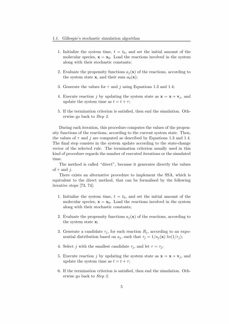
1.1. Gillespie’s stochastic simulation algorithm
1. Initialize the system time, t = t0, and set the initial amount of themolecular species, x = x0. Load the reactions involved in the systemalong with their stochastic constants;
2. Evaluate the propensity functions aj(x) of the reactions, according tothe system state x, and their sum a0(x);
3. Generate the values for τ and j using Equations 1.3 and 1.4;
4. Execute reaction j by updating the system state as x = x + vj, andupdate the system time as t = t + τ ;
5. If the termination criterion is satisfied, then end the simulation. Oth-erwise go back to Step 2.
During each iteration, this procedure computes the values of the propen-sity functions of the reactions, according to the current system state. Then,the values of τ and j are computed as described by Equations 1.3 and 1.4.The final step consists in the system update according to the state-changevector of the selected rule. The termination criterion usually used in thiskind of procedure regards the number of executed iterations or the simulatedtime.
The method is called “direct”, because it generates directly the valuesof τ and j.
There exists an alternative procedure to implement the SSA, which isequivalent to the direct method, that can be formalised by the followingiterative steps [73, 74]:
1. Initialize the system time, t = t0, and set the initial amount of themolecular species, x = x0. Load the reactions involved in the systemalong with their stochastic constants;
2. Evaluate the propensity functions aj(x) of the reactions, according tothe system state x;
3. Generate a candidate τj , for each reaction Rj, according to an expo-nential distribution based on aj, such that τj = 1/aj(x) ln(1/rj);
4. Select j with the smallest candidate τj, and let τ = τj;
5. Execute reaction j by updating the system state as x = x + vj, andupdate the system time as t = t + τ ;
6. If the termination criterion is satisfied, then end the simulation. Oth-erwise go back to Step 2.
5
Chapter 1. Stochastic algorithms for the simulation of biochemical systems
This procedure is called first reaction method, the main difference fromthe direct method is that here M different random numbers, where M is thenumber of reactions, are needed at each iteration, in order to compute thevalue of τ .
In general, SSA has many advantages with respect to other (standard)simulation algorithms, such as: (1) the procedure, that is logically equivalentto the CME, is exact and takes full account of the stochastic fluctuationsof the system; (2) the length of the step τ is exact and not a finite ap-proximation of some infinitesimal dt, as the time step increment used, forinstance, by ODEs solvers; (3) the procedure is very easy to codify, and itdoes not depend on the set of reactions involved in the system. The amountmemory required for a simulation is typically small, i.e., it is proportionalto the number of molecular species and chemical reactions; (4) while theCME tries to solve the system simultaneously for the probability of all pos-sible trajectories, SSA generates a single trajectory, therefore it can easierdescribe the dynamics of a system; (5) by using a number of independentruns of SSA, it is easy to calculate means, variances, correlations, etc. of thespecies involved in the system. Note that, these ensemble averages cannotbe readily computed using the CME.
On the other hand, SSA also presents weaknesses: (1) the computationaltime required to run a single simulation, which is proportional to the numberof reactions M , is usually high because of the sequential execution of asingle reaction at each iterative step; (2) the computational time is alsoproportional to the number of molecules involved in a system, hence, thereis a limitation either in the molecular amounts which can be considered, or inthe total simulation time which can be considered during each execution; (3)the ensemble averages that can be computed from a number of independentsimulations is typically very time consuming. Hence, the statistical accuracyis directly dependent on the time required to execute the simulations.
SSA has been used for the simulation of many biological and chemicalsystems. The earliest application of the SSA to a real biological systemdemonstrating that stochasticity can play a critically important role hasbeen presented in [123], where a model of the mechanism controlling genetranscript and translation has been analysed. Another SSA application re-gards the study of the effect of fluctuations in gene expression rates and othermolecular–level fluctuations on lysis or lysogeny pathway selection statisticsby phage λ–infected Escherichia coli cells [6].
1.2 The next reaction method
In this section, a procedure developed by Gibson and Bruck [72] for theoptimisation of the SSA, will be presented. This algorithm, called nextreaction method (NRM), overcomes one of the main limitations of SSA,
6
1.2. The next reaction method
that is, its applicability to systems with a large number of molecular speciesand chemical reactions. In fact, in such cases the computational time ofSSA usually becomes prohibitively long.
The NRM is based on the method introduced by Gillespie and it is exactas the SSA, though it is more efficient than SSA. NRM exploits the firstreaction method, however, instead of using a random number for each re-action (at each iteration), it assigns a single random number per reactionevent. Moreover, the efficiency of the method relies both on the data struc-tures used to store the propensity function values and the drawn randomnumbers, and on the way they are updated, when needed. Note that, theimprovements due to the use of these data structures can be also extendedto the Gillespie’s direct method.
The aim of NRM is to avoid the execution of three particular operationsrepeated at each iteration of the first reaction method: the update of therandom numbers associated to the reaction events, the computation of thecandidate τi related to each reaction, and the identification of the smallestvalue, among τi’s, which represents the actual τ .
The main idea is to store the values of τi along with the values of thepropensity functions ai of the reactions, and to recalculate the values of ai
(and of the corresponding τi) only if they change. To realise this optimisedupdate operation, a dependency graph is used. This data structure indicateswhich is the relation between reactions and propensity functions, namely,it indicates which propensity functions are affected by the execution of areaction.
The values of τi which are not affected by the reaction executed during aniteration are not modified and re-used at the next iteration. In general, therandom numbers used during Monte Carlo simulations cannot be re-used;nevertheless, in this particular case it is legitimate, as proved in [72]. Hence,all the τi, except for τj (used for the selected reaction), will be re-used. Notethat, so doing, only a few values of both ai and τi will be updated at eachiteration, therefore it is suitable to use an efficient data structure to store thevalues and to update them (when needed). This structure is called indexedpriority queue.
Hereafter, the definitions of dependency graph and indexed priority que-ue will be provided.
In order to define the dependency graph of a chemical system, the iden-tification of reactants and products, of a given reaction, is needed. Given thereaction Ri, these two sets of molecular species will be called reactants(Ri)and products(Ri), respectively. For instance, let us consider the reactionRi : A + B → C, then reactants(Ri) = A,B and products(Ri) = C.Moreover, the set of molecular species which affect the value of ai is calleddependsOn(ai). Note that, usually dependsOn(ai) = reactants(Ri), butthere are cases in which some additional information can be added. Fi-nally, the set of molecular species whose quantities are changed after a rule
7
Chapter 1. Stochastic algorithms for the simulation of biochemical systems
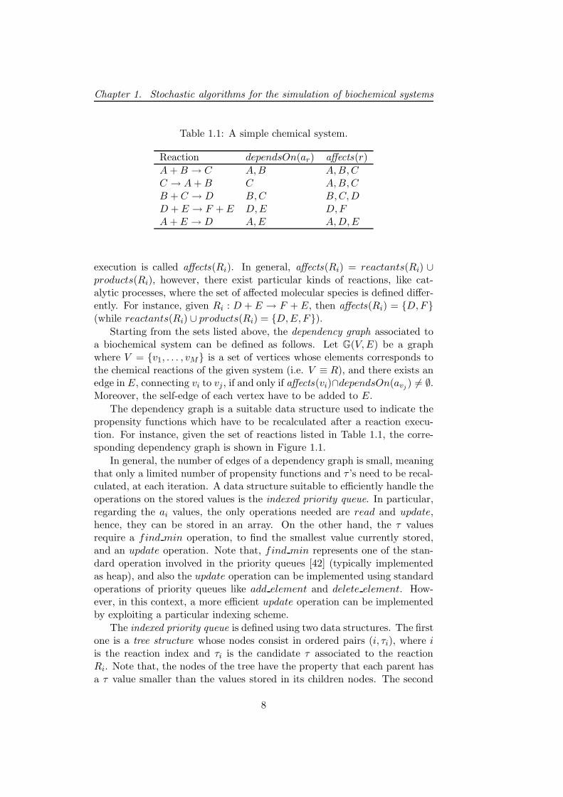
Table 1.1: A simple chemical system.
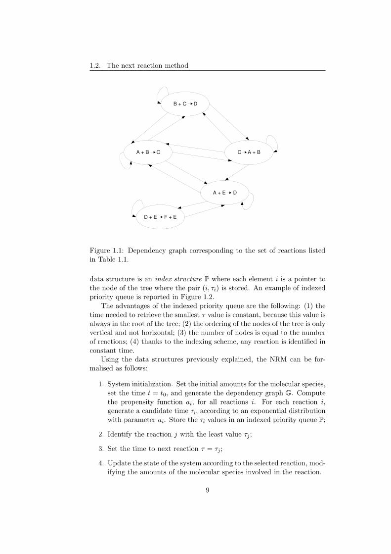
Reaction dependsOn(ar) affects(r)
A + B → C A,B A,B,CC → A + B C A,B,CB + C → D B,C B,C,DD + E → F + E D,E D,FA + E → D A,E A,D,E
execution is called affects(Ri). In general, affects(Ri) = reactants(Ri) ∪products(Ri), however, there exist particular kinds of reactions, like cat-alytic processes, where the set of affected molecular species is defined differ-ently. For instance, given Ri : D + E → F + E, then affects(Ri) = D,F(while reactants(Ri) ∪ products(Ri) = D,E,F).
Starting from the sets listed above, the dependency graph associated toa biochemical system can be defined as follows. Let G(V,E) be a graphwhere V = v1, . . . , vM is a set of vertices whose elements corresponds tothe chemical reactions of the given system (i.e. V ≡ R), and there exists anedge in E, connecting vi to vj , if and only if affects(vi)∩dependsOn(avj
) 6= ∅.Moreover, the self-edge of each vertex have to be added to E.
The dependency graph is a suitable data structure used to indicate thepropensity functions which have to be recalculated after a reaction execu-tion. For instance, given the set of reactions listed in Table 1.1, the corre-sponding dependency graph is shown in Figure 1.1.
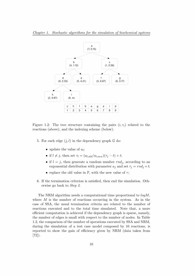
In general, the number of edges of a dependency graph is small, meaningthat only a limited number of propensity functions and τ ’s need to be recal-culated, at each iteration. A data structure suitable to efficiently handle theoperations on the stored values is the indexed priority queue. In particular,regarding the ai values, the only operations needed are read and update,hence, they can be stored in an array. On the other hand, the τ valuesrequire a find min operation, to find the smallest value currently stored,and an update operation. Note that, find min represents one of the stan-dard operation involved in the priority queues [42] (typically implementedas heap), and also the update operation can be implemented using standardoperations of priority queues like add element and delete element. How-ever, in this context, a more efficient update operation can be implementedby exploiting a particular indexing scheme.
The indexed priority queue is defined using two data structures. The firstone is a tree structure whose nodes consist in ordered pairs (i, τi), where iis the reaction index and τi is the candidate τ associated to the reactionRi. Note that, the nodes of the tree have the property that each parent hasa τ value smaller than the values stored in its children nodes. The second
8
1.2. The next reaction method
Figure 1.1: Dependency graph corresponding to the set of reactions listedin Table 1.1.
data structure is an index structure P where each element i is a pointer tothe node of the tree where the pair (i, τi) is stored. An example of indexedpriority queue is reported in Figure 1.2.
The advantages of the indexed priority queue are the following: (1) thetime needed to retrieve the smallest τ value is constant, because this value isalways in the root of the tree; (2) the ordering of the nodes of the tree is onlyvertical and not horizontal; (3) the number of nodes is equal to the numberof reactions; (4) thanks to the indexing scheme, any reaction is identified inconstant time.
Using the data structures previously explained, the NRM can be for-malised as follows:
1. System initialization. Set the initial amounts for the molecular species,set the time t = t0, and generate the dependency graph G. Computethe propensity function ai, for all reactions i. For each reaction i,generate a candidate time τi, according to an exponential distributionwith parameter ai. Store the τi values in an indexed priority queue P;
2. Identify the reaction j with the least value τj;
3. Set the time to next reaction τ = τj;
4. Update the state of the system according to the selected reaction, mod-ifying the amounts of the molecular species involved in the reaction.
9
Chapter 1. Stochastic algorithms for the simulation of biochemical systems
Figure 1.2: The tree structure containing the pairs (i, τi) related to thereactions (above), and the indexing scheme (below).
5. For each edge (j, l) in the dependency graph G do:
• update the value of al;
• if l 6= j, then set τl = (al,old/al,new)(τj − t) + t;
• if l = j, then generate a random number rndj, according to anexponential distribution with parameter aj and set τj = rndj + t;
• replace the old value in P, with the new value of τ ;
6. If the termination criterion is satisfied, then end the simulation. Oth-erwise go back to Step 2.
The NRM algorithm needs a computational time proportional to logM ,where M is the number of reactions occurring in the system. As in thecase of SSA, the usual termination criteria are related to the number ofreactions executed and to the total time simulated. Note that, a moreefficient computation is achieved if the dependency graph is sparse, namely,the number of edges is small with respect to the number of nodes. In Table1.2, the comparison of the number of operations executed by SSA and NRM,during the simulation of a test case model composed by 10 reactions, isreported to show the gain of efficiency given by NRM (data taken from[72]).
10
1.3. The tau-leaping algorithm
Table 1.2: Comparison of SSA and NRM in terms of number of operationexecuted (all numbers are in millions).
Operation SSA NRM
ai computation 2700 210× and ÷ ops 0 340+, − and comparisons 2900 1100exp rnd numbers 35 35uni rnd numbers 35 0
An example of application of the NRM has been presented in [71], wherea Lambda model related to gene transcription and translation, protein–protein interactions and feedback via protein–DNA binding has been simu-lated and analysed.
1.3 The tau-leaping algorithm
The tau-leaping algorithm was first introduced in [77] to the aim of speedingup stochastic simulations of biochemical systems. Instead of simulating thedynamics of the system by tracing every single reaction event occurringinside the volume Ω, with tau-leaping a time increment τ is computed and acertain number of reactions are selected and executed in parallel. So doing,faster simulations can be performed, though the obtained dynamics of thechemical system is not exact, as in SSA, but it is approximated.
Several different versions of the tau-leaping algorithm have been pro-posed, aimed at improving the procedure to compute the τ value and toselect the reactions to be applied in the current step, avoiding the possibilityto obtain negative population of chemical species (we refer to [78, 35, 25] formore details). Despite the improvements in the simulation method achievedby these techniques, they all present a problem related to the description ofthe system dynamics: though an error control parameter is used, they donot allow to uniformly bound the changes of the species quantities duringthe τ selection procedure, therefore resulting in a poor approximation ofthe system dynamics. Moreover, in order to compute the time incrementat each step, they require the evaluation of a quadratic number of auxiliaryquantities (relative to the number of chemical reactions).
These problems have been worked out in the tau-leaping version pre-sented in [26], which will be considered hereafter. As already said, the aimof this procedure is to fire more than one reaction for each time increment[t, t + τ) in order to speed up the simulations. The determination of theexact probability distribution of the reactions applications, within a generic
11
Chapter 1. Stochastic algorithms for the simulation of biochemical systems
step of length τ , is a hard task to solve. Therefore, in order to obtain anefficient numerical realisation of the system’s trajectory, the exact dynamicsof the system has to be approximated.
Given the state x of the system, let Kj(τ,x, t) be the exact number oftimes that a reaction Rj will be fired in the time interval [t, t + τ), so thatK(τ,x, t) is the exact probability distribution vector (having Kj(τ,x, t) aselements). For arbitrary values of τ , it is difficult to compute the values ofKj(τ,x, t). On the contrary, if τ is small enough that the change in the sys-tem’s state during [t, t+τ) is so slight that no propensity function will sufferan appreciable change in its value (this is called the leap condition), thenwe can evaluate a good approximation of Kj(τ,x, t) by using the Poissonrandom variable with mean and variance aj(x)τ .
So, after the computation of a τ value that satisfies the leap condition,it is possible to update the state of the system at time t + τ according to:
X(t + τ) = x +M∑
j=1
vjPj(aj(x), τ) (1.5)
where Pj(aj(x), τ), with j = 1, . . . ,M , denotes an independent sample ofthe Poisson random variable with mean and variance aj(x)τ .
Each iterative step of the tau-leaping procedure is based on four mainstages:
1. Generate the maximum changes of each species that satisfy the leapcondition.
2. Compute the mean and variance of the changes of the propensity func-tions.
3. Calculate the τ value.
4. Sample the reactions numbers to apply.
Hereafter, we describe in detail the motivations and the aims of each ofthe four stages.1. Satisfying the leap condition. The procedure for the selection ofτ is accomplished in order to bound the relative changes in the molecularamounts, in such a way that the relative changes in the propensity functionswill be all bounded - during the τ interval - by a small value ε (0 ≤ ε ≤ 1).
Let ∆τXi be the change in the amount Xi of species Si, during the timeinterval [t, t + τ). Given the state x and its projections xi = Xi(t), the leapcondition can be formalised as:
|∆τXi| ≤ maxεixi, 1 with i = 1, . . . , N , (1.6)
where the values εi = εi(ε, xi) are chosen so that the relative changes in thepropensity functions will be all bounded, at least, by ε.
12
1.3. The tau-leaping algorithm
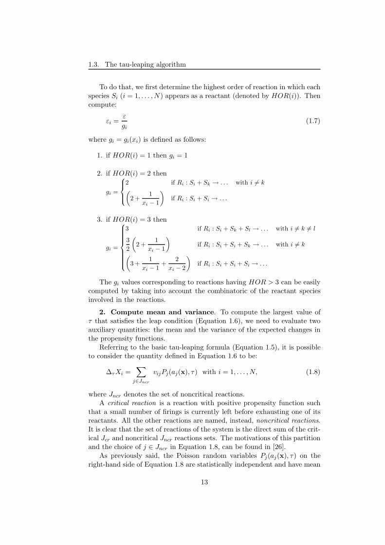
To do that, we first determine the highest order of reaction in which eachspecies Si (i = 1, . . . , N) appears as a reactant (denoted by HOR(i)). Thencompute:
εi =ε
gi(1.7)
where gi = gi(xi) is defined as follows:
1. if HOR(i) = 1 then gi = 1
2. if HOR(i) = 2 then
gi =
2 if Ri : Si + Sk → . . . with i 6= k(
2 +1
xi − 1
)if Ri : Si + Si → . . .
3. if HOR(i) = 3 then
gi =
3 if Ri : Si + Sk + Sl → . . . with i 6= k 6= l
3
2
(2 +
1
xi − 1
)if Ri : Si + Si + Sk → . . . with i 6= k
(3 +
1
xi − 1+
2
xi − 2
)if Ri : Si + Si + Si → . . .
The gi values corresponding to reactions having HOR > 3 can be easilycomputed by taking into account the combinatoric of the reactant speciesinvolved in the reactions.
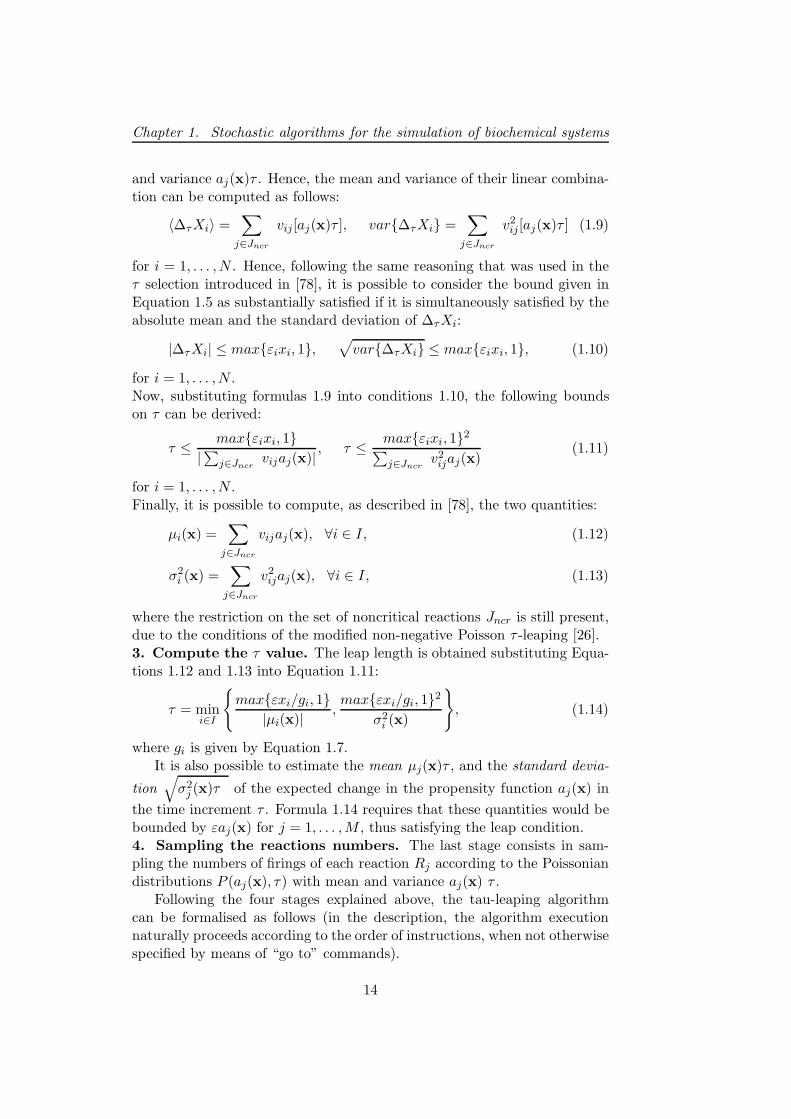
2. Compute mean and variance. To compute the largest value ofτ that satisfies the leap condition (Equation 1.6), we need to evaluate twoauxiliary quantities: the mean and the variance of the expected changes inthe propensity functions.
Referring to the basic tau-leaping formula (Equation 1.5), it is possibleto consider the quantity defined in Equation 1.6 to be:
∆τXi =∑
j∈Jncr
vijPj(aj(x), τ) with i = 1, . . . , N, (1.8)
where Jncr denotes the set of noncritical reactions.A critical reaction is a reaction with positive propensity function such
that a small number of firings is currently left before exhausting one of itsreactants. All the other reactions are named, instead, noncritical reactions.It is clear that the set of reactions of the system is the direct sum of the crit-ical Jcr and noncritical Jncr reactions sets. The motivations of this partitionand the choice of j ∈ Jncr in Equation 1.8, can be found in [26].
As previously said, the Poisson random variables Pj(aj(x), τ) on theright-hand side of Equation 1.8 are statistically independent and have mean
13
Chapter 1. Stochastic algorithms for the simulation of biochemical systems
and variance aj(x)τ . Hence, the mean and variance of their linear combina-tion can be computed as follows:
〈∆τXi〉 =∑
j∈Jncr
vij[aj(x)τ ], var∆τXi =∑
j∈Jncr
v2ij[aj(x)τ ] (1.9)
for i = 1, . . . , N . Hence, following the same reasoning that was used in theτ selection introduced in [78], it is possible to consider the bound given inEquation 1.5 as substantially satisfied if it is simultaneously satisfied by theabsolute mean and the standard deviation of ∆τXi:
|∆τXi| ≤ maxεixi, 1,√
var∆τXi ≤ maxεixi, 1, (1.10)
for i = 1, . . . , N .Now, substituting formulas 1.9 into conditions 1.10, the following boundson τ can be derived:
τ ≤maxεixi, 1
|∑
j∈Jncrvijaj(x)|
, τ ≤maxεixi, 1
2
∑j∈Jncr
v2ijaj(x)
(1.11)
for i = 1, . . . , N .Finally, it is possible to compute, as described in [78], the two quantities:
µi(x) =∑
j∈Jncr
vijaj(x), ∀i ∈ I, (1.12)
σ2i (x) =
∑
j∈Jncr
v2ijaj(x), ∀i ∈ I, (1.13)
where the restriction on the set of noncritical reactions Jncr is still present,due to the conditions of the modified non-negative Poisson τ -leaping [26].3. Compute the τ value. The leap length is obtained substituting Equa-tions 1.12 and 1.13 into Equation 1.11:
τ = mini∈I
maxεxi/gi, 1
|µi(x)|,maxεxi/gi, 1
2
σ2i (x)
, (1.14)
where gi is given by Equation 1.7.It is also possible to estimate the mean µj(x)τ , and the standard devia-
tion√
σ2j (x)τ of the expected change in the propensity function aj(x) in
the time increment τ . Formula 1.14 requires that these quantities would bebounded by εaj(x) for j = 1, . . . ,M , thus satisfying the leap condition.4. Sampling the reactions numbers. The last stage consists in sam-pling the numbers of firings of each reaction Rj according to the Poissoniandistributions P (aj(x), τ) with mean and variance aj(x) τ .
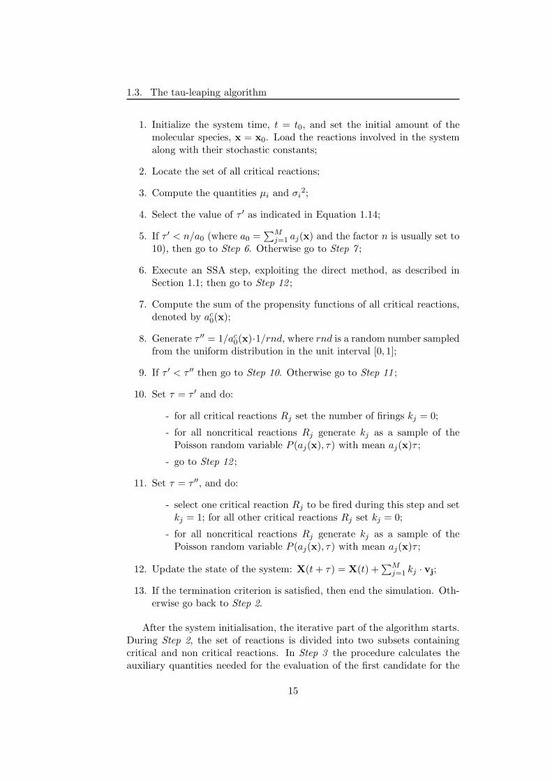
Following the four stages explained above, the tau-leaping algorithmcan be formalised as follows (in the description, the algorithm executionnaturally proceeds according to the order of instructions, when not otherwisespecified by means of “go to” commands).
14
1.3. The tau-leaping algorithm
1. Initialize the system time, t = t0, and set the initial amount of themolecular species, x = x0. Load the reactions involved in the systemalong with their stochastic constants;
2. Locate the set of all critical reactions;
3. Compute the quantities µi and σi2;
4. Select the value of τ ′ as indicated in Equation 1.14;
5. If τ ′ < n/a0 (where a0 =∑M
j=1 aj(x) and the factor n is usually set to10), then go to Step 6. Otherwise go to Step 7 ;
6. Execute an SSA step, exploiting the direct method, as described inSection 1.1; then go to Step 12 ;
7. Compute the sum of the propensity functions of all critical reactions,denoted by ac
0(x);
8. Generate τ ′′ = 1/ac0(x)·1/rnd, where rnd is a random number sampled
from the uniform distribution in the unit interval [0, 1];
9. If τ ′ < τ ′′ then go to Step 10. Otherwise go to Step 11 ;
10. Set τ = τ ′ and do:
- for all critical reactions Rj set the number of firings kj = 0;
- for all noncritical reactions Rj generate kj as a sample of thePoisson random variable P (aj(x), τ) with mean aj(x)τ ;
- go to Step 12 ;
11. Set τ = τ ′′, and do:
- select one critical reaction Rj to be fired during this step and setkj = 1; for all other critical reactions Rj set kj = 0;
- for all noncritical reactions Rj generate kj as a sample of thePoisson random variable P (aj(x), τ) with mean aj(x)τ ;
12. Update the state of the system: X(t + τ) = X(t) +∑M
j=1 kj · vj;
13. If the termination criterion is satisfied, then end the simulation. Oth-erwise go back to Step 2.
After the system initialisation, the iterative part of the algorithm starts.During Step 2, the set of reactions is divided into two subsets containingcritical and non critical reactions. In Step 3 the procedure calculates theauxiliary quantities needed for the evaluation of the first candidate for the
15
Chapter 1. Stochastic algorithms for the simulation of biochemical systems
length of the leap τ ′ (performed in Step 4 ), which is the largest value thatsatisfies the leap condition.
During Step 5, the algorithm checks if the execution of a tau-leaping stepis allowed. In fact, if τ ′ is less than a multiple of 1/a0, then an SSA stepis executed because, given the actual state of the system, it will be moreaccurate and efficient than a tau-leaping step.
In case of the execution of a tau-leaping step, the algorithm proceeds toStep 7 for the computation of the sum of the propensity functions of thecritical reactions, and then to Step 8 to evaluate the second candidate forthe length of the leap τ ′′.
During Step 9 the procedure compares the values of τ ′ and τ ′′. If τ ′
is the smallest one, than only non critical reactions will be selected forthis iteration (Step 10 ). Otherwise, besides non critical reactions, also onecritical reaction will be randomly extracted during the current iteration(Step 11 ).
Finally, in Step 12 the system state is updated and in Step 13 the termi-nation criterion is checked, and if the condition holds, then the execution isterminated. Usually, the termination criteria regards the number of iterationexecuted or the total time simulated.
This version of the tau-leaping algorithm requires a computational timeproportional to 2M (where M is the number of reactions of the system),which corresponds to the number of auxiliary quantities needed for the com-putation of the τ value. Note that, this τ selection strategy is faster thanthat of the original tau-leaping algorithm [77], whereby M2 auxiliary quanti-ties needed to be computed. Moreover, the tau-leaping procedure presentedin this section is also faster than the SSA and the NRM, because it executeslarger steps in which several reactions are applied, thus speeding up thesimulations (as reported in [77, 26, 76]).
The tau-leaping algorithm has been used, for instance, to investigate thecell cycle of the unicellular budding yeast Saccharomyces cerevisiae [1], andto study a model that describes the expression of LacZ and LacY genes andactivity of LacZ and LacY proteins in E. coli.
1.4 The next subvolume method
In this section, an algorithm called next subvolume method (NSM) [57], willbe introduced. This procedure is suitable for the description of the dynamicsof systems whose geometry is taken into account, and both reactive anddiffusive processes are modelled.
This algorithm has been developed starting from the basic proceduresintroduced to give an exact Monte Carlo realisation of the CME describinghomogeneous systems enclosed in a single volume (in particular, the NRM).Note that, a system can be considered homogeneous (that is, the well stirred
16
1.4. The next subvolume method
assumption in SSA, presented in Section 1.1), only if the time scale of thediffusive processes is much more faster than the time scale of the reactiveprocesses.
The aim of the NSM is to propose an algorithm for the description ofsystems where the diffusion plays an important role for the system dynam-ics, e.g. the living cell. As a matter of fact, many cellular processes dependon the spatial heterogeneity [182], as, for instance, the cell division [90]. Inorder to describe the spatial heterogeneity, the NSM divides the reaction vol-ume in a number of subvolumes and exploits the reaction-diffusion masterequation (RDME) to describe the behaviour of the entire system [68]. Thestate of the system is characterised by the amounts of the molecular speciesoccurring within each subvolume, whose dimension is chosen small enoughto be considered homogeneous (well stirred). The diffusive processes amongsubvolumes are described by means of first-order reactions which representthe “movement” of molecules between adjacent subvolumes. The rate con-stant associated to these processes is D/l2, where D is the diffusion constantof a particular molecular species, and l is the side length of the subvolume(whose shape is considered cubic).
Note that, in the case of biochemical systems modelled using a 3D struc-ture, in which chemical processes are faster than diffusive ones, even if thesubvolumes used in the RDME are small, the number of molecules occurringwithin them is usually high, in order to ensure the homogeneity. Therefore,it is not possible to use the SSA inside each subvolume, in order to applya reaction within a single volume, at each iteration. Indeed, the computa-tional time required for the simulation would be prohibitive, as it increaseslinearly with the number of subvolumes used in the system description.
On the other hand, the NSM is an efficient algorithm for the descriptionof 3D biochemical systems, as it can sample trajectories of the Markovprocess associated to the RDME. Moreover, the equivalence between thetrajectories obtained by means of NSM and those sampled by SSA, has beenproven [57]. Hence, the NSM is an exact algorithm capable of describingthe dynamics of heterogeneous systems, designed according to the RDME,and its efficiency (with respect to SSA) is due to the time needed for acomputation, which increases logarithmically, rather than linearly, with thenumber of subvolumes.
The improvements in the performance of this algorithm rely entirelyon the application of the direct method [74], to compute the time for thenext reaction or diffusion event within each subvolume, combined with thestrategy used in the NRM to keep track of the subvolume where the nextevent will occur. Stated in other words, the direct method is used to managethe internal state of the subvolume and to compute the auxiliary valuesneeded for the computation of the time step τ , and to identify the reactionor the diffusion event to execute. On the other hand, the queue of thesubvolumes, the ordering and the update processes are managed using the
17
Chapter 1. Stochastic algorithms for the simulation of biochemical systems
same data structures and operations introduced in the NRM (the indexedpriority queue implemented as a binary tree together with the indexingscheme, see Section 1.2 and [72] for additional details). Note that, duringeach iteration of the NSM, only one subvolume (for reaction events) or twosubvolumes (for diffusion events) need to be updated, because their internalstate changes.
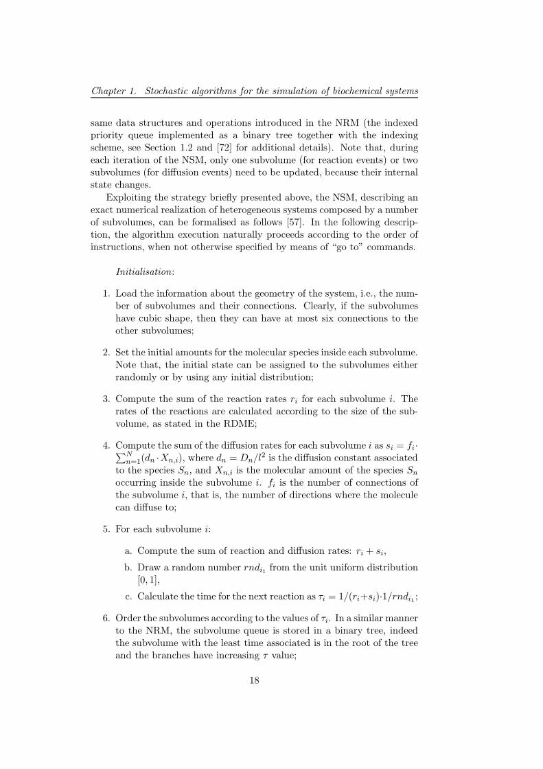
Exploiting the strategy briefly presented above, the NSM, describing anexact numerical realization of heterogeneous systems composed by a numberof subvolumes, can be formalised as follows [57]. In the following descrip-tion, the algorithm execution naturally proceeds according to the order ofinstructions, when not otherwise specified by means of “go to” commands.
Initialisation:
1. Load the information about the geometry of the system, i.e., the num-ber of subvolumes and their connections. Clearly, if the subvolumeshave cubic shape, then they can have at most six connections to theother subvolumes;
2. Set the initial amounts for the molecular species inside each subvolume.Note that, the initial state can be assigned to the subvolumes eitherrandomly or by using any initial distribution;
3. Compute the sum of the reaction rates ri for each subvolume i. Therates of the reactions are calculated according to the size of the sub-volume, as stated in the RDME;
4. Compute the sum of the diffusion rates for each subvolume i as si = fi ·∑Nn=1(dn ·Xn,i), where dn = Dn/l2 is the diffusion constant associated
to the species Sn, and Xn,i is the molecular amount of the species Sn
occurring inside the subvolume i. fi is the number of connections ofthe subvolume i, that is, the number of directions where the moleculecan diffuse to;
5. For each subvolume i:
a. Compute the sum of reaction and diffusion rates: ri + si,
b. Draw a random number rndi1 from the unit uniform distribution[0, 1],
c. Calculate the time for the next reaction as τi = 1/(ri+si)·1/rndi1 ;
6. Order the subvolumes according to the values of τi. In a similar mannerto the NRM, the subvolume queue is stored in a binary tree, indeedthe subvolume with the least time associated is in the root of the treeand the branches have increasing τ value;
18
1.4. The next subvolume method
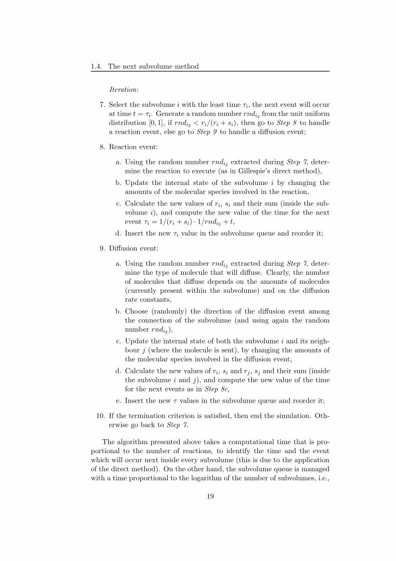
Iteration:
7. Select the subvolume i with the least time τi, the next event will occurat time t = τi. Generate a random number rndi2 from the unit uniformdistribution [0, 1], if rndi2 < ri/(ri + si), then go to Step 8 to handlea reaction event, else go to Step 9 to handle a diffusion event;
8. Reaction event:
a. Using the random number rndi2 extracted during Step 7, deter-mine the reaction to execute (as in Gillespie’s direct method),
b. Update the internal state of the subvolume i by changing theamounts of the molecular species involved in the reaction,
c. Calculate the new values of ri, si and their sum (inside the sub-volume i), and compute the new value of the time for the nextevent τi = 1/(ri + si) · 1/rndi2 + t,
d. Insert the new τi value in the subvolume queue and reorder it;
9. Diffusion event:
a. Using the random number rndi2 extracted during Step 7, deter-mine the type of molecule that will diffuse. Clearly, the numberof molecules that diffuse depends on the amounts of molecules(currently present within the subvolume) and on the diffusionrate constants,
b. Choose (randomly) the direction of the diffusion event amongthe connection of the subvolume (and using again the randomnumber rndi2),
c. Update the internal state of both the subvolume i and its neigh-bour j (where the molecule is sent), by changing the amounts ofthe molecular species involved in the diffusion event,
d. Calculate the new values of ri, si and rj , sj and their sum (insidethe subvolume i and j), and compute the new value of the timefor the next events as in Step 8c,
e. Insert the new τ values in the subvolume queue and reorder it;
10. If the termination criterion is satisfied, then end the simulation. Oth-erwise go back to Step 7.
The algorithm presented above takes a computational time that is pro-portional to the number of reactions, to identify the time and the eventwhich will occur next inside every subvolume (this is due to the applicationof the direct method). On the other hand, the subvolume queue is managedwith a time proportional to the logarithm of the number of subvolumes, i.e.,
19
Chapter 1. Stochastic algorithms for the simulation of biochemical systems
the time needed to re-order the queue is proportional to the logarithm ofthe number of subvolumes.
A different implementation of the NSM could be used to speed up theprocedure, at the cost of using a larger amount of memory. The idea is toexecute the operations within the subvolumes by exploiting the NRM. Sodoing, the computational time needed to handle each subvolume is propor-tional to the logarithm of the number of reactions. On the contrary, insteadof storing only the time τ for the next event, all the candidate values of τneed to be stored. Therefore, the amount of memory required for this al-ternative implementation is proportional to the number of events (for eachsubvolume).
The NSM has been used, for instance, for the simulation of the stochas-tic reaction–diffusion kinetics of a double–negative feedback system, and aMAPK phosphorylation–dephosphorylation system [57].
1.5 The binomial tau-leap spatial stochastic sim-ulation algorithm
The binomial tau-leap spatial stochastic simulation algorithm (Bτ -SSSA)has been introduced in [117], as an alternative procedure to the next sub-volume method for the simulation of heterogeneous systems. The Bτ -SSSAfollows the principles introduced in the NSM, but the algorithm has beenmodified in order to simulate the behaviour of the subvolumes following thethe binomial tau-leap algorithm [196].
In this section, the binomial tau-leap will be briefly recalled, empha-sizing the differences with Gillespie’s tau-leaping (in particular, the versionintroduced in [77] will be considered here); afterwards, the Bτ -SSSA will bedescribed.
One of the main problems of the first version of tau-leaping algorithm,as proposed in [77], concerns the robustness of the method, because theselection and execution of a number of reactions could lead to negativeamounts of the molecular species occurring inside the system. To be moreprecise, during a tau-leaping step (which is usually larger than a SSA step), ifthe number of reactions to fire is greater than the number of molecules of thecurrent system configuration, then negative populations are generated, andthe simulation step cannot be executed. The solution proposed to avoid thispossibility consists in undoing the last step, reducing the length of the stepby half, and selecting a new set of reactions to execute. It is clear that suchkind of solution increases the computational cost of the algorithm, hencedifferent but less expensive methods are needed (note that, the tau-leapingversion presented in Section 1.3 uses a different strategy to efficiently selectboth the time step and the rules, avoiding the negative population problem).
The method proposed in the binomial tau-leap to select the leap length
20
1.5. The binomial tau-leap spatial stochastic simulation algorithm
and reactions consists in the exploitation of binomial random variablesrather than Poisson random variables. This different sampling is suitable forthe tau-leaping because, while samples from Poisson random variables rangefrom zero to infinity, binomial random variables have a finite range. The bi-nomial tau-leap method, besides providing a different sampling, implementsa robust control strategy to avoid negative molecular amounts.
The procedure used to tackle the problem related to negative numbersconsists in bounding the sampling range of the binomial random variablesaccording to the system state. In particular, the number of execution ofa given reaction Rj , during the current iteration, is defined by a samplevalue of the binomial random variable B(Nj , aj(x)/Nj) under the followingcondition:
0 ≤aj(x)τ
Nj≤ 1,
where the value Nj is computed according to the kind of reaction. For in-
stance, given a first-order reaction R1 : S1c1→ S2 (whose propensity function
is a1(x) = c1 ·X1), the value N1 = X1. Dealing with second-order reactions,
in the heterologous case, R2 : S1 + S2c2→ S3 (where a2(x) = c2 ·X1 ·X2) the
value N2 = minX1,X2. In the homologous case of second-order reactions,
such as R3 : S1 + S1c3→ S2 (having a3(x) = c3 · X1(X1−1)
2 ), the reaction isexecutable if X1 ≥ 2 and N3 = ⌊X1/2⌋. It is clear that, for each reactionRj , the number Nj is used to ensure the applicability of the reaction itself,given the current system state x.
The limitation on the number of reactions execution explained above isnot enough to avoid the problem related to the negative molecular numbersif a species is involved in more than one reaction. Therefore, a differentsampling method (based on binomial random variables), has been proposed.This novel strategy is founded on two properties of the Poisson and binomialrandom variables [196], which are exploited to limit the total number ofexecutions of the reactions that modify the molecular quantity of a particularspecies. This sampling method can be explained considering two reactionsRj and Rk which modify the amount of species Si (note that, this procedurecan be easily extended to higher numbers of simultaneous reactions).
Following the (Poisson) tau-leaping procedure [77], the number of execu-tions for reactions Rj and Rk in [t, t+τ) would be sampled from the Poissonrandom variables Pj = P (aj(x)τ) and Pk = P (ak(x)τ), respectively. On theother hand, using the binomial tau-leap, and exploiting the first propertyof Poisson and binomial random variables, the total number of reactionsRj and Rk to execute during the leap is first generated from the binomialrandom variable:
21
Chapter 1. Stochastic algorithms for the simulation of biochemical systems
B
(Ni,
aj(x)
aj(x) + ak(x)τ
)(1.15)
under the following conditions:
Ni = minNj, Nk, 0 ≤aj(x) + ak(x)
Niτ ≤ 1,
where the values Nj and Nk are computed as illustrated above, accordingto the Xi quantity in the state x.
Afterwards, a second sample Kj , which corresponds to the number ofexecutions of reaction Rj can be generated, exploiting the second propertyof Poisson and binomial random variables, from a distribution which dependson the value Kjk, that is, the total number of executions of reactions Rj andRk:
B
(Kjk,
aj(x)
aj(x) + ak(x)
).
Finally, the number of executions of reaction Rk is computed as Kk =Kjk − Kj .
This strategy is exploited in the Bτ -SSSA procedure, whenever a tau-leaping step is executed in one of the subvolumes of the system.
The Bτ -SSSA has been developed in order to speed up the NSM, apply-ing several reaction and diffusive events at each step. During each iterationof the algorithm, a subvolume is selected according to its state (hence, tothe probability values of the corresponding reactions) and the procedure toevolve its state is executed. The first operation consists in computing τ : ifthis value is greater than a specified threshold, then the Bτ -SSSA procedureis applied; otherwise, a modified version of the NSM is performed (executinga single event).
The Bτ -SSSA, where the probabilities associated to both reaction anddiffusion events are calculated as described in Section 1.4, can be formalisedas follows [117]. In the following description, the algorithm execution nat-urally proceeds according to the order of instructions, when not otherwisespecified by means of “go to” commands.
Initialisation:
1. Load the information about the geometry of the system, i.e., the num-ber of subvolumes and their connections;
2. Set the initial amounts for the molecular species inside each subvolume;
22
1.5. The binomial tau-leap spatial stochastic simulation algorithm
3. Compute the sum of the reaction rates ri and the sum of the diffusionrates si within each subvolume i;
4. For each subvolume i, compute the value τi in which the next set ofevents will be executed;
5. Order the subvolumes according to the values of τi;
Iteration:
6. Select the subvolume i with the least τi value;
7. If the total number of molecules occurring inside the subvolume islarger than 2, then go to Step 8. Otherwise proceed with a singleevent iteration step:
a. If ri = 0, then go to Step 11 to execute a single diffusion event;
b. If ri > 0, then draw a random number rnd1. If rnd1 < ri/(ri+si),then go to Step 10 to execute a reaction event. Otherwise go toStep 11 to execute a diffusion event;
8. Calculate an initial τi for the subvolume, as described in [196];
9. Determine whether the step consists of one event or a set of events.In the case of ri > 0, if τi is smaller than a specified threshold, thengo to Step 7b. Otherwise go to Step 12 ;
10. Single chemical reaction event:
a. Draw a random number from the uniform interval [0, 1] to selectwhich reaction will be executed (following the Gillespie’s method[74]);
b. Update the molecular quantities inside the subvolume i accordingto the stoichiometry of the reaction executed, and increase thesimulation time;
c. Update the values of ri and si inside the subvolume i;
d. Generate a new τi value for the next event inside volume i andsort the subvolume queue;
e. If the termination criterion is satisfied, then end the simulation.Otherwise go back to Step 6.
11. Single diffusion event:
a. Draw a random number from the uniform interval [0, 1] to selectwhich species will diffuse to a neighbour subvolume (following theNSM method [57]);
23
Chapter 1. Stochastic algorithms for the simulation of biochemical systems
b. Draw a random number from the uniform interval [0, 1] to selectthe neighbour subvolume j where the molecule will diffuse;
c. Update the molecular quantities inside the subvolumes i and jaccording to the executed diffusion event, and increase the simu-lation time;
d. Update the values of the reaction and diffusion events probabili-ties inside the subvolumes i and j;
e. Generate new τi and τj values for the next event inside volume iand j and sort the subvolume queue;
f. If the termination criterion is satisfied, then end the simulation.Otherwise go back to Step 6.
12. τ -leap step:
a. Select the reaction and diffusion events according to the strategyof the binomial tau-leap presented above [196];
b. Update the system state according to the set of selected reactionand diffusion events, and update the system time;
c. Calculate the new values of the propensity functions in the sub-volumes affected by the executed events;
d. Generate new τ values and sort the subvolume queue;
e. If the termination criterion is satisfied, then end the simulation.Otherwise go back to Step 6.
As in the first version of Gillespie’s tau-leaping algorithm [77], the Bτ -SSSA needs the evaluation of M2 auxiliary quantities to compute the lengthof the step τ , inside the selected subvolume. Exploiting a modified version ofthe NSM to manage the subvolumes, the algorithm presented here inheritsthe same computational time (described in Section 1.4). Comparing thenumber of operations needed to execute one iteration of the NSM and theBτ -SSSA, it turns out that the latter has a higher complexity. On the otherhand, the Bτ -SSSA executes a set of reaction and diffusion events (at eachstep), instead of a single event, increasing the efficiency of the simulations.In particular, in [117] it is reported that the Bτ -SSSA is from 2 to 100 timesfaster than NSM (depending on the number of subvolumes involved in themodelled system), in the examples presented by the authors.
The Bτ -SSSA has been exploited for simulating a simplified model ofprogesterone transcription factor formation in the epidermal growth factorreceptor pathway using different numbers of subvolumes in the system’sdefinition [117].
24
1.6. Other algorithms
1.6 Other algorithms
In the last years, many other stochastic algorithms have been proposed forthe simulation of biochemical systems. In this section, we recall some ofthese works giving a brief explanation of their features.
R-leaping. An algorithm called R-leaping [7] has been proposed for theacceleration of the SSA, by executing a predefined number of reaction firingswhich may occur across several reactions, with the aim to avoid the prob-lem related to the possible occurrence of negative populations of molecules(which is present in most of the tau-leaping methods [77, 35, 196]). At eachiteration of the R-leaping algorithm, assuming that the values of the propen-sity functions remain constant during the leap (as for tau-leaping [77]), avalue representing the total number of reactions firings is computed. Thisvalue is used to extract the number of execution of each reaction by meansof binomial distribution samples.
The authors demonstrate that, by periodically sorting the reactions, suchthat the propensity functions result in decreasing order, it is possible tominimize the number of sampling from the binomial distributions, withoutaffecting the accuracy of dynamics described by the algorithm.
The bound on the total number of reaction executions is given as aparameter of the algorithm. Anyway, the strict limit can be relaxed inorder to simulate larger steps, allowing the occurrence of negative amountsaccording to a controlled probability value. This relaxation strategy offersa tuning mechanism to balance accuracy and efficiency of the R-leapingaccording to the system state.
The R-leaping algorithm is approximately 10 times faster than SSA [74],and has the same accuracy level of tau-leaping [26], as reported in [7]; how-ever, the computation time required for the execution of the R-leaping isgreater than that needed by the tau-leaping.
The R-leaping has been applied to a LacZ/LacY model composed by 22reactions providing good results from the simulations.
Stochastic simulation of coupled reaction–diffusion processes. Theclassic stochastic algorithms have been developed for the simulation of nonlinear chemical reaction processes in well stirred homogeneous systems. In[189], one of the first stochastic approaches which consider diffusion for nonlinear reaction–diffusion processes has been introduced. In order to handlediffusion processes, mesoscopic rates used to describe the transition proba-bility associated to diffusive events have been added to the described system.
Exploiting the mesoscopic rates associated to diffusion, the algorithmprovides a numerical simulation, by means of a Monte Carlo technique, ofthe reaction-diffusion master equation. The described dynamics considersboth the spatial and temporal evolution of the molecular species occurring
25
Chapter 1. Stochastic algorithms for the simulation of biochemical systems
inside the system. As in other methods like NSM and Bτ -SSSA, here thereaction volume is divided in subvolumes, called voxels, which are supposedto be homogeneous.
This algorithm is limited to reaction–diffusion processes where collisionsbetween inert and reacting species occur more frequently than collisions be-tween reacting species. Moreover, the authors do not give any insight aboutthe computational cost of the algorithm, which seems to have a higher com-plexity with respect to the NSM or the Bτ -SSSA, because of the auxiliaryquantities needed to compute the value of the time step τ .
This method has been applied, for instance, to the nonlinear reaction–diffusion process of calcium wave propagation through the cell, the devel-oped model consists in 100 sequential cubic voxels since diffusion has beenconsidered in one dimension only [189].
Next reaction hybrid algorithm. In [179], a stochastic algorithm suit-able for the description of chemical systems having one or more “fast” re-actions, is presented. Such kind of systems, called stiff systems, cannot beefficiently described by means of SSA, because the average length of the stepτ might be very small, slowing down the simulation. The paper describes ahybrid stochastic method that partitions the system into subsets of fast andslow reactions. The dynamics of fast reactions can be accurately approx-imated as a continuous Markov process when two conditions are satisfied:(1) reactions occur many time in a small time interval, and (2) the effect ofeach reaction execution on the number of reactants and products is small,that is, the total amounts of those molecular species have to be large. Onthe other hand, the slow dynamics governed by slow reactions is describedby using the next reaction method. There exists other approaches with theaim to efficiently simulate stiff systems: the slow scale SSA and the implicittau-leaping [76].
The next reaction hybrid method has been successfully applied to severalbiochemical systems, such as the pulse generator, a simplified model of themolecular mechanisms responsible for the circadian rhythm in Drosophilafruit flies. However, there are two main sources of inaccuracy for this al-gorithm: the first one is due to the approximation of fast reactions as acontinuous Markov process, in particular, this is related to the inaccuracy ofthe numerical integration method used (here, the Euler-Maruyama method).The authors propose the application of a more advanced stochastic numer-ical integrator to reduce this source of the error.
The second source of inaccuracy appears when a slow reaction is influ-enced by some changes in the molecular quantities of species involved ina fast reaction. In this case the source of error is related to the stochasticnumerical integrator used to generate the times associated to slow reactions;again, by using more advanced methods the accuracy of the algorithm might
26
1.6. Other algorithms
be improved.
Multicompartmental Gillespie’s algorithm. This algorithm has beenintroduced in [159] to simulate systems composed by many volumes (alsocalled compartments), exploiting the Gillespie’s procedure. In particular,the direct method is used for the computation of the time τ and the indexof the next reaction to execute within each compartment. This informationis stored in a list which is updated at each iteration, modifying the valuesrelated to the compartments affected by the executed reaction. This strat-egy is very similar to that of the NSM, presented in Section 1.4, with thedifference that the multicompartmental Gillespie’s algorithm does not use aparticular data structure such as a heap or an indexed queue to efficientlyhandle compartments information.
In the description of biochemical systems modelled by means of thismethod, the so called boundary rules are exploited. Such kind of reactionsare used to capture the features of the communication and the transfor-mation of molecules. In particular, the authors consider special cases ofboundary rules which involve molecules occurring in different compartments,though it is not very clear how Gillespie’s theory for single volume systemscan be used to describe the propensity functions of reactions that are si-multaneously active in two compartments, nor in which compartment thisinformation is used to compute the value of τ .
27

Chapter 1. Stochastic algorithms for the simulation of biochemical systems
28
Chapter 2
Optimization algorithms
In this chapter two optimization techniques will be presented: genetic al-gorithms and particle swarm optimizer. These optimisation methods canbe applied in the field of modelling and simulation of biological and chem-ical systems since many numerical factors, like molecular quantities andreaction rates, which represent an indispensable quantitative information toperform computational investigations of the system’s behaviour, are oftennot available or inaccurate. Optimization methods can be used to tackle thecalibration problem of parameter estimation of these systems by minimizinga cost function (e.g. a distance measure) which quantitatively defines howgood is the system behaviour using the predicted values, with respect to theexperimental dynamics. In Chapter 6 the parameter estimation issue, andthe application of genetic algorithms and particle swarm optimizer to thisparticular problem will be described.
Genetic Algorithms (GAs) [89] are one of the oldest and mostly usedversions of evolutionary algorithms. The most commonly used GAs formu-lation evolves fixed length strings of characters from a limited alphabet, butthere exists other versions where each allele contains any floating point valuefrom a limited range. This GAs version is often called real valued or realcoded GAs [204].
In Section 2.1, an introduction to the basic features of GAs is given. Af-terwards, binary coded GAs and real coded GAs, along with their commonlyused variation operators, are presented.
Particle swarm optimizer (PSO) [99] is a population based optimisationheuristic, inspired by the social behaviour of bird flocking or fish school-ing. In PSO the potential solutions, called particles, are identified by theircoordinates in the problem space and are characterized by a velocity thatallows them to update their current positions. The PSO concept consistsin changing, at each iteration, the velocity of each particle towards someattractors, in order to reach optimal positions in the search space.
In Section 2.2, the basic notions of PSO are explained. Moreover, an
29
Chapter 2. Optimization algorithms
analysis of the role of the algorithm’s parameters involved in the velocityupdate operation is given.
2.1 Genetic algorithms
Genetic algorithms are search methods which exploit principles inspired byevolutionary theories, to the aim of evolving candidate solutions for a givenproblem and finding optimal solution [89, 79]. Solutions are arranged in apopulations of individuals which evolve by means of competition and con-trolled variation. The individuals compete in a process called selection,which is executed according to a quality measure (fitness). Hence, indi-viduals with higher fitness will be selected with higher probability. Newindividuals are then generated starting from the selected ones, by apply-ing genetic operators called crossover and mutation, which mix the parentscharacteristics, and introduce new genetic material, respectively.
One of the reasons why GAs succeed in optimization problems is due totheir capability to exploit the information accumulated about an initiallyunknown search space, and adapt the individuals in order to conduct suc-cessive explorations within useful subspaces. GAs are therefore suitable forlarge and complex search spaces, where other “classical” search approachesare inappropriate. GAs offer a valid method to optimize problems thatrequire (computationally) efficient and effective techniques.
In this section, two GAs version will be presented: binary-coded GAs andreal-coded GAs. We start with a brief overview about GAs, explaining thecommon features of the two versions. GAs are initialised with a populationof individuals that are usually randomly generated, each one correspond-ing to a potential solution of the given problem. During each iteration,also called generation, the quality of the individuals is evaluated througha fitness function, and the individuals for the next generations are finallyselected, recombined and variated. A general implementation for GAs canbe formalised as follows:
1. Initialise the system by randomly generating an initial population ofindividuals;
2. Evaluate the fitness function for each individual;
3. Select the individuals for the next generation;
4. Recombine and vary the selected individuals;
5. If the termination criterion is satisfied, then end the procedure. Oth-erwise go back to Step 2.
The algorithm reported above represents one possible variants of GAs,however, all the implementations for these algorithms are based on the same
30
2.1. Genetic algorithms
fundamental mechanism for the evolution of the individuals, which consistsin three operations: evaluation of the fitness function, selection of the bestperforming individuals, and recombination of the characteristics of the se-lected individuals. Clearly, the execution of a GA terminates when somecriterion is satisfied. For instance, a termination criterion can be related tothe number of iteration executed, or to the best value of the fitness functionobtained from an individual.
Evaluation of the fitness function. The fitness function used to evalu-ate the quality of each individual is independent from the implemented GAsversion. On the other hand, the fitness evaluation strongly depends on theoptimization problem to which the GAs are applied, and on the representa-tion used for the individuals.
GAs are commonly applied to function optimisation problems, in whichthe aim is to find a set of parameter values that maximise a complex mul-tiparameter function. Hereafter, we report a simple example where the aimis to maximise the real–values one–dimensional function
f(y) = y + |sin(32y)|, 0 ≤ y < π.
The candidate solutions of this problem are the values of y, which can beencoded by means of binary strings representing real numbers. The fitnessfunction can be defined in order to translate a given binary string x (anindividual) into a real number y, and then to evaluate the function at thatvalue. Clearly, in this case the fitness value of x corresponds to the functionvalue evaluated at the point y.
In Section 6.3, a fitness function developed and applied to the problemof parameter estimation of biochemical systems will be described.
Selection of the best performing individuals. Given a population Pof N individuals i, i = 1, . . . , N , (N is also called the size of P ), the selectionprocedure is used to obtain an intermediate population P ′ which is composedby copies of individuals from P . The number of copies of an individual addedto P ′ is directly dependent on its fitness value. Individuals with higherfitness generally have greater chance to be selected for the intermediatepopulation.
There exist different selection strategies, the first we present here is calledroulette wheel selection [89, 79], a procedure where the selection of individ-uals is proportional to their fitness values. For each individual i in P , theprobability pi of including a copy of i to P ′ is computed as:
pi =fi∑N
j=1 fj
.
31
Chapter 2. Optimization algorithms
The selection procedure can be imagined as the spinning of a roulettewheel a number of times equal to the size of the population; clearly, thenumber of fittest individuals added to P ′ will be higher than the numberof the weakest individuals. So doing, individuals with fitness values aboveaverage will be more represented in the next generations, while individualsbelow average fitness tend to extinct.
The second selection approach recalled here is the ranking selection [8].The individuals are first sorted according to their fitness values, and then thecomputation of pi is based on the rank of i (rather than on its fitness value),by using a non-increasing assignment function. The ranking selection is usedwhen a balancing (or unbalancing) between strong and weak individuals isrequired.
The last selection procedure here described is called tournament selection[131]. This kind of selection is performed by executing a number of “tour-naments” equal to the size of the population. During each tournament, afew individuals are randomly selected from P , and the winner, that is, theindividual with the best fitness among them, is added to the intermediatepopulation P ′. The number of participants to the tournament (k) is directlyrelated to the selection pressure. In fact, if k is large, then weak individualshave a smaller probability to be selected for P ′. Note that, if k = 1, thetournament selection is equivalent to a random selection of the individuals,where each individual has the same probability to be included in P ′. The in-dividuals selected by means of a tournament can be removed from P , unlessit is feasible that the same individuals is allowed to participate to distincttournaments and be selected many times for the intermediate population.The tournament selection has several advantages: (1) the fitness evaluationof the entire population is not required, indeed, only the individuals selectedfor the tournaments are evaluated; (2) it is easy to code and can be executedon parallel architectures; (3) the selection pressure can be easily adjusted(by changing the value of k).
Recombination of the characteristics of the selected individuals.After the construction of the intermediate population P ′ by means of anyselection procedure, the variation operators can be applied in order to obtainnew individuals (offspring) for the next generation.
The first operator applied is called crossover, it is used to mix the infor-mation between individuals. Crossover combines the features of two parentindividuals, with the aim to obtain two offspring with better characteristics.This operator plays a central role in GAs, and is considered one of the mostcharacterising feature of this optimization technique. In general, crossoveris not applied to all selected pairs of individuals: its application dependson a probability value pc, called crossover rate. Moreover, different versionsof crossover can be defined according to the representation chosen for the
32
2.1. Genetic algorithms
individuals.
The second operator is called mutation, whose aim is to arbitrarily alterone or more components (allele) of a selected individual, in order to increasethe variability inside the new generation. Mutation introduces new geneticmaterial into the population, preventing the convergence of the individualsto local optimal solutions, and it ensures that the probability to reach everypoint in the search space is always greater than zero. Similarly to crossover,the mutation operator is applied with a probability pm, called mutation rate;hence, a randomly selected allele of each individual undergoes a change ofits value according to pm.
Typically, the parameter setting for these operators is chosen such thatcrossover is applied with high probability values (for instance, 0.95), andmutation is executed with very low rates (like 0.05), in order to reflect thenatural evolution process where usually the characteristics of two individualsare mixed through, e.g., sexual reproduction, while mutations happen withvery low probability.
The application of these variation operators might lead to the extinctionof the best individual of the population, either because it gets mixed withanother individual or because of the mutation of one of its allele. Hence,after the construction of the intermediate population P ′, it is possible toapply an additional selection strategy, called elitism [46], to “copy” the bestindividual (or a subset of best individuals) into the population of the nextgeneration without modifying it.
Binary–coded GAs
The first version of GAs, which we present now, exploits a binary coding torepresent the individuals of the population. Given the search space S, thepoints in S are codified by means of strings over the alphabet V = 0, 1,having fixed-length L. For instance, a GA with population size equal to 5and individual length equal to 7, can be randomly initialised as:
i1 = 0100101i2 = 1101010i3 = 1111000i4 = 0100110i5 = 1000000
As previously explained, after the fitness evaluation of the individu-als and the selection procedure to obtain the intermediate population P ′,crossover and mutation are applied.
The classical crossover operator for binary coded GAs is named sim-ple crossover [89, 79]. Given two individuals ij = (a1
j , . . . , aLj ) and ik =
(a1k, . . . , a
Lk ) randomly chosen from P ′, two offspring i′j = (a1
j , . . . , acj , ac+1
k ,
. . . , aLk ) and i′k = (a1
k, . . . , ack, a
c+1j , . . . , aL
j ) are generated. The crossover
33
Chapter 2. Optimization algorithms
point c is randomly selected from the uniform interval [1, . . . , L − 1].
There exist different kinds of crossover. Among the most important ones,we recall: (1) n-points crossover [60], which represents a generalisation ofsimple crossover, since n different crossover points are randomly selected andthe resulting segments of the parents individuals are exchanged to generatethe offspring; (2) uniform crossover [190], where the value of each allele inthe offspring is determined by the uniform random choice between the valuesof the corresponding allele in the parents.
The mutation operator [89, 79] is applied to an individual by randomlychoosing an allele and swapping its value (from 1 to 0 or vice versa).
Many advantages are given by the use of binary alphabets in GAs. Firstof all, this alphabet maximizes the level of implicit parallelism, as explainedin [80]. This property is related to the useful implicit information processed“in parallel” by GAs, such as schemata (besides the explicit informationrepresented by the individuals). Moreover, the use of a binary alphabetprovides a benefit in terms of computational cost. Indeed, when alphabetswith higher cardinality are used, a larger population size is often neededin order to well represent every character [172], thus resulting in a loss ofefficiency (especially when the fitness function computation is expensive).
On the other hand, the binary representation of individuals is not suit-able when dealing with a continuous complex search space with large di-mensions, and when a high numerical precision is required. Furthermore,when an individual can only assume a finite number of discrete valid values(which is not a power of 2), some of the binary values are redundant.
Real–coded GAs
The second version of GAs briefly described here utilises a real coding forthe individuals. In this case, each allele is codified as a real number whichrepresents a variable of an optimization problem with values in continuousdomains. Therefore, the individual is implemented as a vector of floatingpoint numbers, whose precision is related to that of the computer with whichthe execution of the algorithm is performed. The size of the individuals isequal to the length of the vector representing a candidate solution to theanalysed problem, hence each allele codifies a variable. The values of theallele are forced to range in the intervals of the corresponding variables, andalso the the values resulting from the application of variation operators haveto follow this requirement.
Given two individuals ij = (a1j , . . . , a
Lj ) and ik = (a1
k, . . . , aLk ), which have
been randomly selected from the intermediate population P ′, the effect of themost used kinds of crossover will be described in the following. Note that,each crossover operator generates a different number of offspring, thereforea strategy called offspring selection mechanism, for deciding which ones willbe included in the next generation, is used in some cases.
34
2.1. Genetic algorithms
The first operator is called flat crossover [169], it generates an offspringio = (a1
o, . . . , aLo ) where the values al
o (l = 1, . . . , L) are randomly chosenfrom the uniform interval [al
j , alk].
Using the simple crossover [204, 129], a position c ∈ 1, 2, . . . , L − 1is randomly chosen and two offspring io1
= (a1o1
, . . . , aco1
, ac+1o2
, . . . , aLo2
) andio2
= (a1o2
, . . . , aco2
, ac+1o1
, . . . , aLo1
) are obtained.
With the arithmetical crossover [129], two offspring ioh= (a1
oh, . . . , aL
oh)
(h = 1, 2) are generated, by computing the values of the allele as alo1
=λal
j +(1−λ)alk and al
o2= λal
k +(1−λ)alj (l = 1, . . . , L). λ is a used–defined
constant (uniform arithmetical crossover) or is updated according to thecurrent generation (non-uniform arithmetical crossover).
Applying the BLX-α crossover [61], an offspring io = (a1o, . . . , a
co, . . . , a
Lo )
is generated; the value aco is a random number sampled from the uniform
interval [amin − I · α, amax + I · α], where amax = maxacj , a
ck, amin =
minacj , a
ck and I = amax − amin.
In the linear crossover [204], three offspring ioh= (a1
oh, . . . , aL
oh) (h =
1, 2, 3) are obtained, where alo1
= 12al
j + 12al
k, alo2
= 32al
j −12al
k and alo3
=
−12al
j + 32al
k. In this case, the offspring selection mechanism is applied withthe aim to select the two most promising offspring.
The operator called discrete crossover [143] generates an offspring io =(a1
o, . . . , aLo ) whose elements al
o are randomly chosen from the set alj , a
lk.
Using the extended line crossover [143], an offspring io = (a1o, . . . , a
co, . . . ,
aLo ) having elements al
o = alj + α(al
k − alj), is generated. The value of α is
randomly chosen from the uniform interval [−0.25, 1.25].
The extended intermediate crossover [143] is slightly different from theprevious one, here an offspring io = (a1
o, . . . , aco, . . . , a
Lo ) having elements
alo = al
j + αl(alk − al
j), is generated. The value of αl is randomly chosen (foreach allele) from the uniform interval [−0.25, 1.25].
The last crossover operator we recall here is the Wright’s heuristic cross-over [204]. Supposing that ij is the parent with the best fitness value, thenthe values of the offspring are computed as al
o = r · (ilj − ilk) + ilj , where r isa random number sampled from the interval [0, 1].
After the application of the crossover operator on the intermediate pop-ulation P ′, the mutation operator is applied. Given an individual i =(a1, . . . , aL), the allele al (whose value ranges in the interval [al
min, almax])
is the value randomly selected that will be mutated, and al is the value ofthe allele after the application of a mutation operator. In what follows, theeffect of different mutation operators will be shown.
Using random mutation [129], al is obtained as a random number drawnfrom the uniform interval [al
min, almax].
Applying the non-uniform mutation [129] in the generation t, with tmax
as the maximum number of generations, then:
35
Chapter 2. Optimization algorithms
al =
al + ∆(t, al
max − al) if τ = 0al − ∆(t, al − al
min) if τ = 1
where τ is a random number whose value can be either 0 or 1, and
∆(t, y) = y(1 − r(1− ttmax
)b
),
where r is a random number sampled from the interval [0, 1], and b is a user–defined parameter which determines how much mutation is dependent on thenumber of iterations. The ∆ function gives a number in the range [0, y] suchthat the probability of returning a number close to zero increases with thenumber of iterations. Therefore, using this operator the mutation is “strong”during the first iterations, achieving a wide range search; conversely, in thelater stage of the algorithm, the mutation is “weak”, resulting in a localtuning of the value.
Another mutation operator is called real number creep [44]. This strat-egy is applied when an individual is in a “good” local maximum, and theexploration of its neighbourhood might be interesting. In order to achievethis, the allele is increased or decreased by a small random quantity sampledfrom a user defined range.
The Muhlenbein’s mutation [143] changes the value of the allele as al =al ± rangl · γ, where rangl indicates the mutation range (and it is usuallyset to 0.1 · (al
max − almin)), and γ =
∑15j=0 αj · 2
−j (where 15 represent theprecision of the operator). The value of α ∈ 0, 1 is randomly generatedwith p(α = 1) = 1
16 . The value of the allele is increased or decreased withprobability 0.5, and ranges in the interval [al − rangl, al + rangl] with aprecision of rangl · 2−15 for the smallest variation.
There exist other crossover and mutation operators for real coded GAs,which are generalisations of the operators presented above or other novelstrategies suitable for convex search spaces. An overview of these methodscan be found in [88].
The advantages of using real coded GAs are many, for instance, theyallow to handle large domains for the involved variables, which is insteaddifficult to achieve by using a binary implementation, where increasing thedomains results in a loss of precision (assuming fixed length individuals).Moreover, the real coding allows a local tuning of the solutions, since smallvariations in the variable values result in slight changes in the (entire) in-dividual. On the contrary, in the binary coding, a swap of a single allelecan produce a completely different individual. Finally, the real coding rep-resentation of the solution is close to the “natural” formulation of manyproblems, hence the encoding and decoding processes, which are necessaryfor binary GAs versions, can be avoided, increasing the algorithm efficiency.
36
2.2. Particle swarm optimizer
GAs have been successfully applied to a wide variety of applications.For instance, GAs can be applied to the field of control systems engineering;indeed, in most of the controller designs, some parameters are required tobe optimized in order to give a better overall control performance. Fur-thermore, the configuration or the order of the controller can be optimizedto reduce the system’s complexity. Another example of GAs applicationregards the patterns recognition. GAs can be applied to generate the im-age filters for a two–stage target recognition system in such a way that thetarget image from background clutter is vividly classified from the imagingdata. GAs can be used in automatic speech recognition systems where thespoken speech patterns (test pattern) are usually identified by using thepre-stored speech patterns (reference patterns). The comparison of speechsignals has a number of difficulties as variations in time and the time scalesamong them are not fixed. Therefore, time registration of the test and thereference patterns is one of the fundamental problems in the area of au-tomatic isolated word recognition. Finally, GAs can be applied to proteinfolding simulations problem. Here, the population consists in conformationsof the polypeptide chain. Then, conformations are changed by mutation, inthe form of conventional Monte Carlo steps, and crossover is executed byinterchanging parts of the polypeptide chain between conformations.
We refer the reader to [113, 200] (and references therein) for additionalinformation about GAs applications.
2.2 Particle swarm optimizer
Particle swarm optimizer (PSO) [99] is a method for the optimization ofcontinuous nonlinear functions, which has been developed simulating sim-plified social behaviours [174], taking inspiration from herds, schools andflocks. The theory behind PSO states that individual members of a schoolcan profit from the discoveries and previous experience of all other membersduring the search of food. This advantage can become decisive, outweighingthe disadvantages of competition for food items, whenever the resource isunpredictably distributed in patches. In other words, this statement indi-cates that social sharing of useful knowledge among members of the samespecies represents a fundamental evolutionary advantage.
In order to simulate the search for food, the members of the swarm (calledparticles) need to be moved within the search space. The movement is ac-complished according to two properties: nearest-neighbour velocity match-ing and “craziness”. The velocity of each member is updated according toits nearest neighbour, resulting in a coordinated movement. So doing, theswarm quickly settles on an unchanging direction. Therefore, a stochasticfactor called “craziness” is used to add a sort of noise to the movement ofthe swarm members.
37
Chapter 2. Optimization algorithms
PSO has the advantage of relying on very simple concepts, making iteasy to implement and computationally inexpensive. Moreover, the perfor-mances of PSO on test functions are comparable to that of GAs, but thisoptimization technique does not suffer from some of the difficulties of GAs:first, the interaction of the group enhances the progress towards the opti-mum solution (while in GAs, interaction by means of crossover can have theopposite effect). PSO has memory, in fact, particles are always attractedby the best positions found so far, because good solutions are stored. Onthe contrary, in GAs, changes result in destruction of previous knowledge,except when “elitism” is applied to the population.
In both PSO and GAs, the initialisation consists in a population of ran-dom solutions to the considered problem. However, PSO’s particles are alsocharacterised by a random velocity, and they can “fly” through the searchspace. As previously said, the particles have memory, since they keep trackof the best solution they have achieved so far; this particular value is calledpersonal best. Another “best” value is traced, according to the PSO versionused, which can be a global best, that is, the best position found so far by theentire swarm, or a local best, namely, the best position found by the neigh-bourhood of the particle. The difference between the “global” and “local”version of PSO, as reported in [54], consists in the fact that using a globalbest information shared among the particles, the average number of itera-tions needed by the swarm to converge to an optimum solution is smaller.Conversely, using a local best strategy, neighbour particles groups sponta-neously separate and explore different regions of the search space, makingthe method more resistant to local optima. The evaluation of the qualityof the particles position is measured by means of a fitness function. Thisfunction is independent from the different PSO versions, but it is strictlyassociated to the optimisation problem to which PSO is applied.
Thanks to the information carried on by particles, PSO (and in general,swarm intelligence) follows five basic principles. First, the proximity prin-ciple, which states that the population should be able to accomplish simplespace and time computations. Second, the quality principle: the populationshould respond to quality factors in the environment. Third, the diverseresponse principle: the population should not behave in a completely coor-dinated manner. Fourth, the stability principle: the behaviour of the pop-ulation should not change every time the environment changes. Fifth, theadaptability principle: the population must change behaviour mode when itis advantageous.
To be more precise, PSO meets the five principles because, first, itconsists of a series of time steps in which n–dimensional computationsare accomplished. Second, the population responds to the personal andglobal/local best quality factors. Third, different influences from the qual-ity factors lead to diverse responses among particles. Fourth, the populationbehaviour changes only when the best position changes. Fifth, the popula-
38
2.2. Particle swarm optimizer
tion is adaptive, in the sense that it does change its behaviour when the bestpositions changes. PSO is defined as a set of N particles, which are placed
in a n–dimensional space. Each coordinate of the particle −→xi (i = 1, . . . , N)is denoted by means of the element xi,d (d = 1, . . . , n). −→pi and −→pg representthe personal best and the global best found so far by the particle −→xi , respec-tively. The vector −→vi denotes the velocity of the particle −→xi and it can rangewithin the interval [−VMax, VMax]. rnd1 and rnd2 are two random numbers.
The basic version of the PSO can be formalised as follows:
1. Initialise the system assigning to each particle a random position andvelocity;
2. For each particle i and for each dimension d do:
• if fitness(i) < besti then pi,d = xi,d;
• vi,d = vi,d + rnd1(pi,d − xi,d) + rnd2(pg,d − xi,d);
• if vi,d > VMax then vi,d = VMax
else if vi,d < −VMax then vi,d = −VMax;
• xi,d = xi,d + vi,d;
3. If the termination criterion is satisfied, then end the procedure. Oth-erwise go back to Step 2.
During the first step, as already stated above, the population is randomlyinitialised in the n–dimensional search space, by assigning a random valueto each coordinate xi,1, . . . , xi,n of the particle −→xi . Moreover, also the initialvelocity −→vi is randomly assigned to the particles.
During each iteration of the algorithm, the position of the particle i istested, in order to quantify its quality by means of a fitness function. If thecurrent position is better than the previous personal best position (−→pi ), thenthe position −→xi is stored in the vector −→pi .
By evaluating all the particles of the swarm, it is also possible to identifythe global or local best position (−→pg). The global best position correspondsto the best performing particle of the entire population, while the local bestposition regards the neighbourhood of a particle. One of the most usedconcept of neighbourhood consists in considering the particles i−1 and i+1for each particle i in the swarm.
The values rnd1 and rnd2 are positive random numbers drawn from theinterval [0, c1] and [0, c2], respectively, which are used to update the particlevelocity. c1 and c2 are system’s parameters, whose value is fixes a priori ofcan vary during the execution, according to the implemented PSO version.The values of the velocity −→vi of the particle −→xi is limited by the value VMax.VMax is used because there are cases in which the particle’s velocity −→vi canincrease without limits, at each iterative step of the algorithm. The value of
39
Chapter 2. Optimization algorithms
VMax can be arbitrarily selected, though it is usually set according to someknowledge of the problem. Otherwise, the value of VMax can be the same ofXMax, which is the search space limit of the particles.
The velocity of a particle is directly influenced by the distance from itspersonal best (−→pi −
−→xi) and from the local/global best (−→pg − −→xi), and theupdated value of −→vi is used during the final stage of step 3 of the algorithm,to change the particle position such that −→xi(t) = −→xi(t − 1) + −→vi (t), thussimulating the movement in the search space toward the best positions foundso far.
During the iterations of the PSO algorithm, better positions found byparticles are substituted into −→p vectors, hence, the population convergestowards optimal regions of the search space. The success of PSO is mainlydue to the interactions among the particles, which influence the trajectoriesduring the exploration of the solutions space.
It is worth noticing that the algorithm works on the values −→vi used toupdate the position of the particles, rather than modifying the positions −→xi
of the particles. In particular, a particle does not move directly towards thebest position, but it will tend to circle around it, because its direction isonly in part influenced by the two system’s attractors, namely, the personaland local/global best positions.
The execution of the PSO terminates when some criterion is satisfied.For instance, a termination criterion can be related to the number of iter-ation executed, or to the best value of the fitness function obtained from aparticle’s position.
The parameters c1 and c2. The trajectory of a particle depends on thec1 and c2 values used during the velocity update process.
As shown in [98], the trajectories that the particles will undertake dur-ing PSO iterations, can be described by analysing the following simplifiedsystem, changing the value of c:
−→vi (t) = −→vi (t − 1) + c(−→pi + −→vi (t − 1))−→xi(t) = −→xi(t − 1) + −→vi (t)
The initial values of −→vi ,−→pi , and −→xi can be arbitrarily set (with −→vi 6= 0).
In the examples below, the system will be initialised with −→xi(0) = −→pi = 0and −→vi (0) = 2.
The value of c has been varied within the range [0, 4]. With c = 0, thetrajectory becomes −→vi (t) = −→vi (t−1), thus the particle continues on its initialdirection in each iteration. Changing the c value in the interval (0, 0.5], theparticle trajectory has a sort of sinusoidal form, as shown in Figure 2.1 (left)where c = 0.1. Increasing the value of the parameter c, the amplitude of thetrajectory decreases, and exceeding the value 0.5, some irregularity in the
40
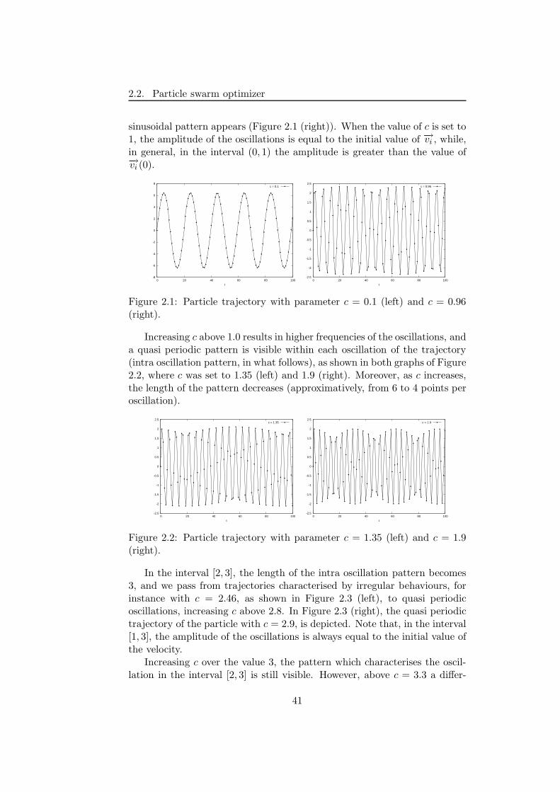
2.2. Particle swarm optimizer
sinusoidal pattern appears (Figure 2.1 (right)). When the value of c is set to1, the amplitude of the oscillations is equal to the initial value of −→vi , while,in general, in the interval (0, 1) the amplitude is greater than the value of−→vi (0).
-8
-6
-4
-2
0
2
4
6
8
0 20 40 60 80 100
t
c = 0.1
-2.5
-2
-1.5
-1
-0.5
0
0.5
1
1.5
2
2.5
0 20 40 60 80 100
t
c = 0.96
Figure 2.1: Particle trajectory with parameter c = 0.1 (left) and c = 0.96(right).
Increasing c above 1.0 results in higher frequencies of the oscillations, anda quasi periodic pattern is visible within each oscillation of the trajectory(intra oscillation pattern, in what follows), as shown in both graphs of Figure2.2, where c was set to 1.35 (left) and 1.9 (right). Moreover, as c increases,the length of the pattern decreases (approximatively, from 6 to 4 points peroscillation).
-2.5
-2
-1.5
-1
-0.5
0
0.5
1
1.5
2
2.5
0 20 40 60 80 100
t
c = 1.35
-2.5
-2
-1.5
-1
-0.5
0
0.5
1
1.5
2
2.5
0 20 40 60 80 100
t
c = 1.9
Figure 2.2: Particle trajectory with parameter c = 1.35 (left) and c = 1.9(right).
In the interval [2, 3], the length of the intra oscillation pattern becomes3, and we pass from trajectories characterised by irregular behaviours, forinstance with c = 2.46, as shown in Figure 2.3 (left), to quasi periodicoscillations, increasing c above 2.8. In Figure 2.3 (right), the quasi periodictrajectory of the particle with c = 2.9, is depicted. Note that, in the interval[1, 3], the amplitude of the oscillations is always equal to the initial value ofthe velocity.
Increasing c over the value 3, the pattern which characterises the oscil-lation in the interval [2, 3] is still visible. However, above c = 3.3 a differ-
41
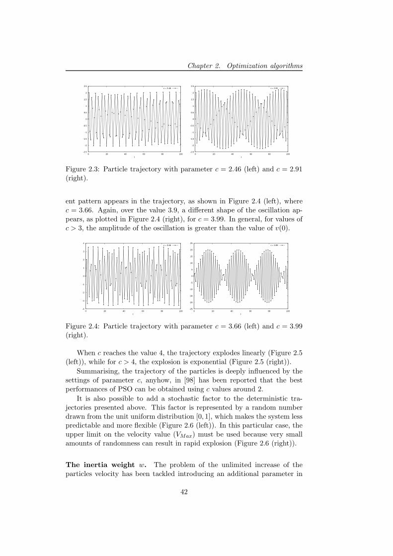
Chapter 2. Optimization algorithms
-2.5
-2
-1.5
-1
-0.5
0
0.5
1
1.5
2
2.5
0 20 40 60 80 100
t
c = 2.46
-2.5
-2
-1.5
-1
-0.5
0
0.5
1
1.5
2
2.5
0 20 40 60 80 100
t
c = 2.91
Figure 2.3: Particle trajectory with parameter c = 2.46 (left) and c = 2.91(right).
ent pattern appears in the trajectory, as shown in Figure 2.4 (left), wherec = 3.66. Again, over the value 3.9, a different shape of the oscillation ap-pears, as plotted in Figure 2.4 (right), for c = 3.99. In general, for values ofc > 3, the amplitude of the oscillation is greater than the value of v(0).
-4
-3
-2
-1
0
1
2
3
4
0 20 40 60 80 100
t
c = 3.66
-25
-20
-15
-10
-5
0
5
10
15
20
25
0 20 40 60 80 100
t
c = 3.99
Figure 2.4: Particle trajectory with parameter c = 3.66 (left) and c = 3.99(right).
When c reaches the value 4, the trajectory explodes linearly (Figure 2.5(left)), while for c > 4, the explosion is exponential (Figure 2.5 (right)).
Summarising, the trajectory of the particles is deeply influenced by thesettings of parameter c, anyhow, in [98] has been reported that the bestperformances of PSO can be obtained using c values around 2.
It is also possible to add a stochastic factor to the deterministic tra-jectories presented above. This factor is represented by a random numberdrawn from the unit uniform distribution [0, 1], which makes the system lesspredictable and more flexible (Figure 2.6 (left)). In this particular case, theupper limit on the velocity value (VMax) must be used because very smallamounts of randomness can result in rapid explosion (Figure 2.6 (right)).
The inertia weight w. The problem of the unlimited increase of theparticles velocity has been tackled introducing an additional parameter in
42
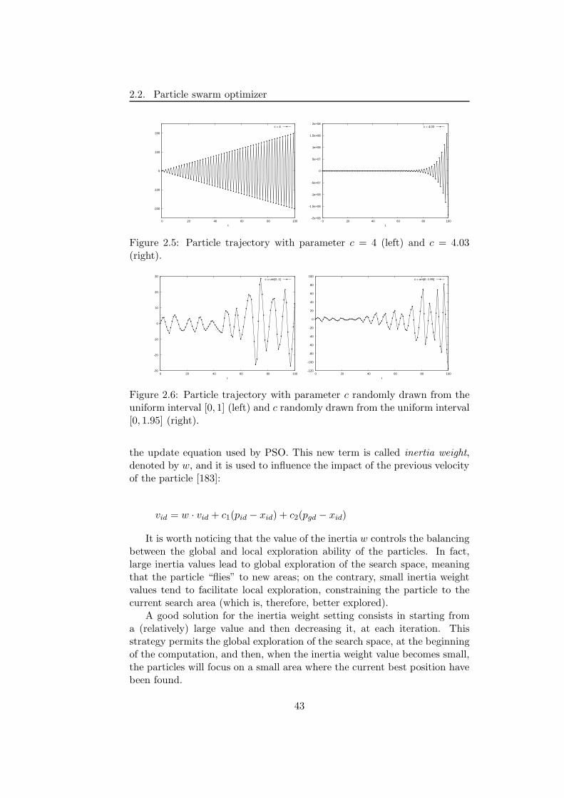
2.2. Particle swarm optimizer
-200
-100
0
100
200
0 20 40 60 80 100
t
c = 4
-2e+08
-1.5e+08
-1e+08
-5e+07
0
5e+07
1e+08
1.5e+08
2e+08
0 20 40 60 80 100
t
c = 4.03
Figure 2.5: Particle trajectory with parameter c = 4 (left) and c = 4.03(right).
-30
-20
-10
0
10
20
30
0 20 40 60 80 100
t
c = urn[0..1]
-120
-100
-80
-60
-40
-20
0
20
40
60
80
100
0 20 40 60 80 100
t
c = urn[0..1.95]
Figure 2.6: Particle trajectory with parameter c randomly drawn from theuniform interval [0, 1] (left) and c randomly drawn from the uniform interval[0, 1.95] (right).
the update equation used by PSO. This new term is called inertia weight,denoted by w, and it is used to influence the impact of the previous velocityof the particle [183]:
vid = w · vid + c1(pid − xid) + c2(pgd − xid)
It is worth noticing that the value of the inertia w controls the balancingbetween the global and local exploration ability of the particles. In fact,large inertia values lead to global exploration of the search space, meaningthat the particle “flies” to new areas; on the contrary, small inertia weightvalues tend to facilitate local exploration, constraining the particle to thecurrent search area (which is, therefore, better explored).
A good solution for the inertia weight setting consists in starting froma (relatively) large value and then decreasing it, at each iteration. Thisstrategy permits the global exploration of the search space, at the beginningof the computation, and then, when the inertia weight value becomes small,the particles will focus on a small area where the current best position havebeen found.
43
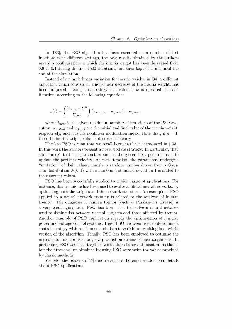
Chapter 2. Optimization algorithms
In [183], the PSO algorithm has been executed on a number of testfunctions with different settings, the best results obtained by the authorsregard a configuration in which the inertia weight has been decreased from0.9 to 0.4 during the first 1500 iterations, and then kept constant until theend of the simulation.
Instead of a simple linear variation for inertia weight, in [34] a differentapproach, which consists in a non-linear decrease of the inertia weight, hasbeen proposed. Using this strategy, the value of w is updated, at eachiteration, according to the following equation:
w(t) =
((tmax − t)n
tnmax
)(winitial − wfinal) + wfinal
where tmax is the given maximum number of iterations of the PSO exe-cution, winitial and wfinal are the initial and final value of the inertia weight,respectively, and n is the nonlinear modulation index. Note that, if n = 1,then the inertia weight value is decreased linearly.
The last PSO version that we recall here, has been introduced in [135].In this work the authors present a novel update strategy. In particular, theyadd “noise” to the c parameters and to the global best position used toupdate the particles velocity. At each iteration, the parameters undergo a“mutation” of their values, namely, a random number drawn from a Gaus-sian distribution N(0, 1) with mean 0 and standard deviation 1 is added totheir current values.
PSO has been successfully applied to a wide range of applications. Forinstance, this technique has been used to evolve artificial neural networks, byoptimising both the weights and the network structure. An example of PSOapplied to a neural network training is related to the analysis of humantremor. The diagnosis of human tremor (such as Parkinson’s disease) isa very challenging area; PSO has been used to evolve a neural networkused to distinguish between normal subjects and those affected by tremor.Another example of PSO application regards the optimisation of reactivepower and voltage control systems. Here, PSO has been used to determine acontrol strategy with continuous and discrete variables, resulting in a hybridversion of the algorithm. Finally, PSO has been employed to optimise theingredients mixture used to grow production strains of microorganisms. Inparticular, PSO was used together with other classic optimisation methods,but the fitness values obtained by using PSO were twice the values providedby classic methods.
We refer the reader to [55] (and references therein) for additional detailsabout PSO applications.
44
Chapter 3
Membrane systems
In this chapter some prerequisites and basic notions of membrane systemswill be recalled. Membrane systems, also called P systems, have been in-troduced as a class of parallel, distributed and nondeterministic comput-ing devices, inspired by the architecture and the functioning of living cells.Many variants of membrane systems have been presented to provide a suit-able modelling framework for chemical, biological and ecological systems[164, 31, 16, 17]. P systems provide a suitable modelling framework forbiological and chemical systems composed of many volumes. Within themembrane defined in the structure of a P system, the set of reaction ofa system can be written by means of rewriting rules, moreover, the com-munication of objects between adjacent volumes can be easily managed byusing special kind of rewriting rules which send objects from one volume toanother one.
A variant of membrane systems, called dynamical probabilistic P systems(DPPs), will be described in this chapter. Differently from the basic def-inition of P systems, in DPPs, probabilities are associated with the rules,and such values vary during the evolution of the system, according to a pre-scribed strategy. Thanks to the probability values, the rules are not appliedin a maximal parallel way, but different level of parallelism can be used,thus allowing a qualitative description of the systems dynamics. DPPs rep-resent the starting point of the development of a novel simulation strategywhich allows the quantitative description of biological and chemical systems(that will be presented in Chapter 4). We present an application of DPPsfor the modelling and simulation of metapopulations, also called multi-patchsystems, which are ecological models used to analyse the behaviour of in-teracting populations, to the aim of determining how a fragmented habitatinfluences local and global population persistence.
45
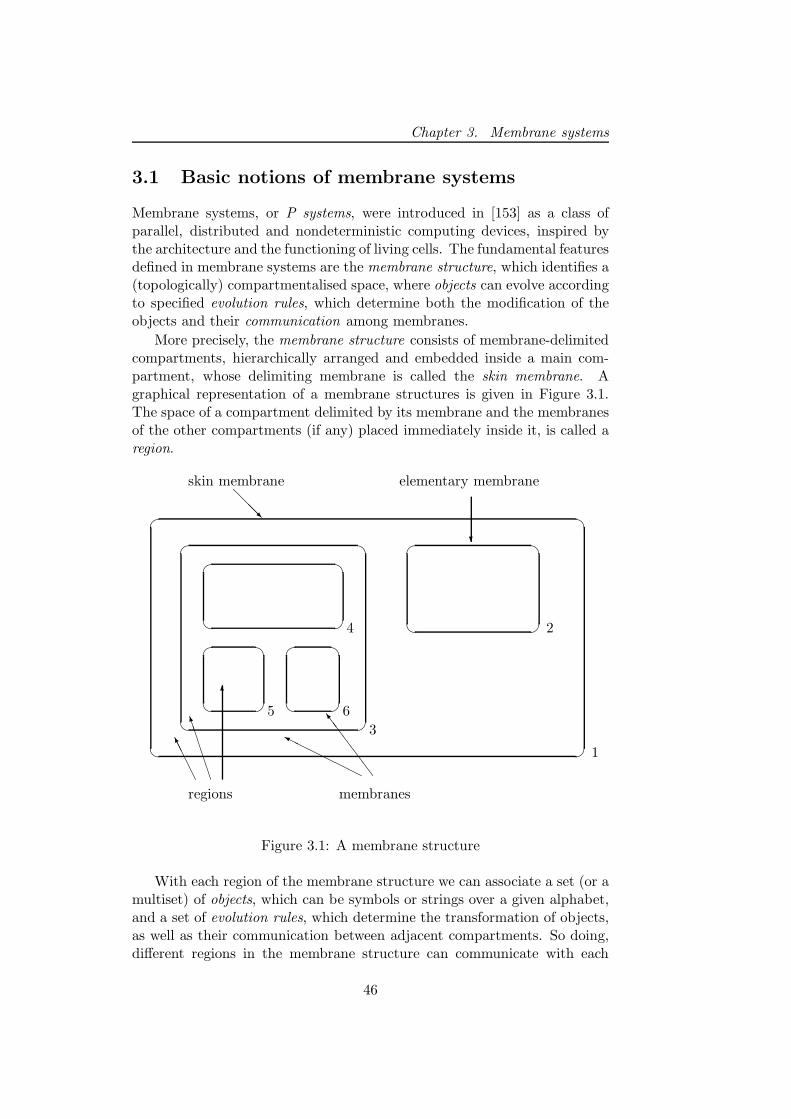
Chapter 3. Membrane systems
3.1 Basic notions of membrane systems
Membrane systems, or P systems, were introduced in [153] as a class ofparallel, distributed and nondeterministic computing devices, inspired bythe architecture and the functioning of living cells. The fundamental featuresdefined in membrane systems are the membrane structure, which identifies a(topologically) compartmentalised space, where objects can evolve accordingto specified evolution rules, which determine both the modification of theobjects and their communication among membranes.
More precisely, the membrane structure consists of membrane-delimitedcompartments, hierarchically arranged and embedded inside a main com-partment, whose delimiting membrane is called the skin membrane. Agraphical representation of a membrane structures is given in Figure 3.1.The space of a compartment delimited by its membrane and the membranesof the other compartments (if any) placed immediately inside it, is called aregion.
?
@@@R
AA
AAK
BB
BBBM
6
SS
SS
So
HHHHHHY
skin membrane elementary membrane
regions membranes
1
2
3
4
5 6
Figure 3.1: A membrane structure
With each region of the membrane structure we can associate a set (or amultiset) of objects, which can be symbols or strings over a given alphabet,and a set of evolution rules, which determine the transformation of objects,as well as their communication between adjacent compartments. So doing,different regions in the membrane structure can communicate with each
46
3.1. Basic notions of membrane systems
other by sending or receiving objects. Usually, the evolution rules are appliedin a nondeterministic and maximally parallel way: all the objects which canevolve should evolve. Moreover, a strict partial order relation can be definedover the set of evolution rules present inside a compartment, indicating apriority relation among them. Due to the application of evolution rules, amembrane can also be dissolved: it disappears from the membrane structure,the set of rules inside that membrane is removed, the set of objects pass tothe outer membrane (which contained the disappeared one). Hence, theevolution rules do not only modify the objects and their placing, but canalso intervene in changing the membrane structure.
An “abstract” interpretation of a P system in biological terms can begiven as follows. The membrane structure corresponds to the organisationof a living cell, of eukaryotic or prokaryotic type (see, e.g., [3]), where thereexists an external membrane (the plasma membrane) and, possibly, some or-ganelles inside the cell, each delimited by a membrane. In each organelle, aswell as inside the cytoplasm, there exist different types of substances (ions,proteins, nucleic acids, etc.) which can be described by means of (multisetsof) symbols or strings. Under specific conditions, these substances are mod-ified by biochemical reactions and they can remain in the same organellewhere they are placed, or selectively cross the membrane which delimits theorganelle. These processes correspond to the way evolution rules are definedand work in P systems: they modify the formal objects (symbols or strings)and also indicate where the modified objects should be at the next step. Thepriority relations above rules can be interpreted as different “reactivities” ofthe biochemical reactions. Moreover, we can also assume that reactions notonly modify chemicals, but also “consumes energy”, thus when a rule witha higher priority is applied, no rule with a lower priority can be used too,because no more energy is available. Some biochemical reactions need thecooperation of catalytic substances, other may be so powerful to cause themembrane lysis. Both events have a natural correspondence in P systems:the use of catalyst objects, and in the dissolving action of rules. When aninternal membrane is “broken” inside a cell, its content is left free in thecytoplasmic space, though the biochemical reactions previously occurring inthat organelle might not take place in the cytoplasm, due to possibly differ-ent chemical and physical conditions (e.g., the pH value). Similarly, whena membrane is dissolved in a P system, its set of rules is removed, but itsobjects still remain in the membrane structure of the system.
A P system is a computing device obtained starting from an initial con-figuration (described by a fixed membrane structure containing a certainnumber of objects and rules) and letting the system evolve. A universalclock is assumed to exist: at each step, all rules from all regions are simulta-neously applied to all objects which can be the subject of an evolution rule.When no further rule can be applied, the computation halts and we get theresult in a prescribed way. On the contrary, if there is at least one rule that
47
Chapter 3. Membrane systems
can be applied forever, then the computation is said to be unsuccessful andno output is obtained.
In the following, the basic definitions of P systems, is given. For furtherdetails and for more information, examples and other variants, we refer to[153, 154, 156, 168].
Formally, the membrane structure can be represented by a string of cor-rectly matching square parentheses, placed in a unique pair of matchingparentheses. Each pair of matching parentheses corresponds to a membraneand, usually, membranes are univocally labelled with distinct numbers. Forinstance, the string µ = [0 [1 ]1 [2 [3 ]3 [4 ]4 ]2 ]0 corresponds to a mem-brane structure consisting of 4 membranes placed at three hierarchical lev-els. Moreover, the same membrane structure can be also represented by thestring µ′ = [0 [2 [4 ]4 [3 ]3 ]2[1 ]1 ]0, that is, any pair of matching parenthe-ses at the same hierarchical level can be interchanged, together with theircontents; this means that the order of pairs of parentheses is irrelevant, whatmatters is their respective relationship.
Each pair of matching parentheses [ ] appearing in a membrane structureµ is called a membrane. The external membrane of a membrane structure iscalled the skin membrane, while a membrane without any other membraneinside (appearing in a membrane structure in the form [ ]) is called anelementary membrane.
The number of membranes in µ is called the degree of µ and it is denotedby deg(µ). The depth of a membrane structure µ, dep(µ), is recurrentlydefined as:
1. if µ = [ ], then dep(µ) = 1;
2. if µ = [µ1 . . . µn], for some membrane structures µ1, . . . , µn, thendep(µ) = 1 + maxdep(µi) | 1 ≤ i ≤ n.
A region is the closed space delimited by a membrane and by the mem-branes immediately inside it (if any). Note that a membrane structure ofdegree n contains exactly n regions, each one associated with a membraneand labelled with the same integer of that membrane. The whole spaceoutside the skin membrane is called the outer region or environment.
Given a finite alphabet V , we can provide a membrane structure µ withsome multisets Mi : V → N, one for each membrane i ∈ 0, . . . , n − 1.
The elements of a multiset are called objects, the multiset present in aregion is called the contents of this region. The total number of objects inan elementary membrane i is called the size of i, denoted by size(i). If amembrane j is placed inside a membrane i and they contribute to identify thesame region (namely, the one delimited by the membrane i), then the objectsinside the region associated with i are said to be adjacent to membrane j.
Finally, the objects occurring inside the regions of a P system can evolve,according to certain specified rules. An evolution rule over an alphabet V
48
3.1. Basic notions of membrane systems
is a pair (u, v), which can be written as u → v, where u is a (non empty)string over the alphabet V and v = v′ or v = v′δ, where v′ is a string overV × (here, out ∪ inj | 0 ≤ j ≤ n − 1), and δ is a special symbol not inV . The length of the string u is called the radius of the rule u → v. Notethat the strings u, v are understood as representations of multisets over V ,in a natural sense.
Given a membrane structure together with multisets and evolution rules,the formal definition [153] of the basic variant of P systems can be given asfollows: a transition P system of degree n, n ≥ 1, is a construction
Π = (V, T,C, µ,M0, . . . ,Mn−1, (R0, ρ0), . . . , (Rn−1, ρn−1), io)
where:
• V is the alphabet of the system;
• T ⊆ V is the terminal (or output) alphabet;
• C ⊆ V,C ∩ T = ∅ is the alphabet of catalysts;
• µ is a membrane structure consisting of n membranes, which are in-jectively labelled by numbers in the set 0, . . . , n − 1;
• M0, . . . ,Mn−1 are multisets over V , representing the objects initiallypresent in the regions 0, . . . , n − 1 of the system;
• R0, . . . , Rn−1 are finite sets of evolution rules associated with the re-gions 0, . . . , n − 1 of µ;
• ρ0, . . . , ρn−1 are strict partial order relations defined over R0, . . . , Rn−1
respectively, specifying a priority relation among the evolution rules;
• io is a number in the set 0, . . . , n − 1 ∪ ∞, indicating the outputregion.
Some more remarks about the definition of a P system are to be given, be-fore explaining its functioning as a computing device. Any multiset M0, . . . ,Mn−1 can be empty, as well as any set of evolution rules R0, . . . , Rn−1, orany strict partial order relation ρ0, . . . , ρn−1.
If Π contains evolution rules whose radius is greater than 1, then it issaid to be cooperative, otherwise it is a non-cooperative system. A particularclass of cooperative systems is that of catalytic systems: whenever the radiusof an evolution rule is strictly greater than 1, then such rule is of the formca → cv, where c ∈ C, a ∈ V \ C, v ∈ (V \ C)∗; moreover, no other rulecontains any catalytic symbols. If C = ∅, then the system is non-catalytic.
According to the strict partial order relation ρi, 0 ≤ i ≤ n − 1, a ruler ∈ Ri is said to be with priority if there exists another rule r′ ∈ Ri such
49
Chapter 3. Membrane systems
that r > r′ or r′ > r. If r is a rule with priority and there is no other ruler′ such that r′ > r, then r is a rule of highest priority. Note that, as ρi is a(strict) partial order relation, there can be more than one rule with highestpriority. A rule r is said to be without priority if it does not appear in ρi.
The (n+1)-tuple (µ,M0, . . . ,Mn−1) constitutes the initial configurationof the system. In general, any sequence of the form (µ′,M ′
i1, . . . ,M ′
ik) con-
stitutes a configuration of Π, where M ′i1
, . . . ,M ′ik
are multisets over V and µ′
is a membrane structure obtained by removing from the original membranestructure µ all membranes different from i1, . . . , ik (and not equal to the skinmembrane), according to the dissolving action which will be explained lateron. The labels i1, . . . , ik of the membranes in µ′ are always numbers in theset 0, . . . , n − 1, corresponding to the initial labels of the membranes inµ, that is, in successive configurations the initial labelling of the membranes(which have not been removed from µ) is never modified.
Given two configurations C1 = (µ′,M ′i1
, . . . ,M ′ik
), C2 = (µ′′,M ′′j1
, . . . ,M ′′
jl) of Π, we write C1 =⇒ C2 and we say that there is a transition from C1
to C2 if we can pass from C1 to C2 by using the evolution rules in R′i1
, . . . , R′ik
using the following prescriptions.All rules are simultaneously examined, in the decreasing order of their
priority (if any), and objects are accordingly assigned to rules. A rule r canbe applied only when there are enough copies of the objects whose evolutionit describes, and which were not “consumed” by rules of higher priority.That is, objects are assigned to the rules which have the highest priorityand, in the case that two or more rules of this type compete for the sameobjects, then the rule to be applied is nondeterministically chosen amongthem. Then, when no more rules with the highest priority can be applied(irrespectively of the objects they involve), the rules with a lower priorityare considered. Again, if there are many rules with the same priority whichcompete for some objects, then the rule to be applied is nondeterministicallychosen among them.
All the objects which can be the subject of evolution rules must be in-volved in the rule application. This use of the priority relations correspondsto the strong interpretation: if a rule with a higher priority is used, then noother rules with less priority can be applied, even if they do not competefor the same objects. Nonetheless, also a weak interpretation of the priorityrules can be considered: a rule with less priority can be applied at the sametime with the rule of higher priority if there are “free” objects which are notinvolved by the rule with the higher priority. The rules without prioritiescan be applied at any time, even together with rules with priorities.
The result of the application of the rule (r : u → v) ∈ R′is
is determinedby v:
• if an object appears in v in the form (a, here), then it remains in thesame region is (the indication here will often be omitted);
50
3.1. Basic notions of membrane systems
• if an object appears in v in the form (a, out), then it exits the mem-brane is and becomes an element of the region immediately outside it.If the membrane is is the skin membrane, then the object leaves thesystem and it will never come back;
• if an object appears in v in the form (a, int) and it is a membraneimmediately inside is, then the object is added to the multiset Mit .If it is not a membrane immediately inside is, then the application ofthe rule is not allowed;
• if the symbol δ appears in v, then membrane is is removed (we sayit is dissolved) from µ′ and, at the same time, the couple (R′
is, ρis) is
erased, the multiset M ′is
is added to the region immediately outsidemembrane is. The dissolving of the skin membrane is never allowed.
All these operations are performed in a maximal parallel mode: in onestep, inside each region all applicable rules u → v are used over all occur-rences of multisets u, and all regions are processed at the same time. Hence,the parallelism is maximal at both a global and a local level: the globallevel involves all membranes at the same time, the local level involves allevolution rules and all objects inside each region.
The functioning of the system as just described defines its nature as acomputing device. Starting from the initial configuration and applying therules in the way described above, we obtain a sequence of transition amongconfigurations: such a sequence is called a computation with respect to Π.A computation is successful if and only if it halts, that is, no rule is furtherapplicable to the objects appearing in any membrane of the system and,if an internal membrane io is specified as the output membrane, then itmust appear in the halting configuration as an elementary membrane. Ifio ∈ 0, . . . , n − 1, then the system is said to work in the internal mode, ,and the result of a successful computation can be read in one of the followingways:
1. if we consider the multiset which is present in the output membrane,then the system is said to generate multisets;
2. if we consider the size of the output membrane, then the system issaid to generate numbers;
3. if certain initial objects ai1 , . . . , aik are specified in advance, and weconsider this occurrences n1, . . . , nk in the output membrane at theend of the computation, then the system is said to generate relations;
4. if a fixed elementary membrane is specified as the input membrane,the system is said to recognise a multiset (the initial contents of theinput membrane), a number (the size of the input membrane) or arelation (the occurrences of certain symbols in the input membrane).
51
Chapter 3. Membrane systems
otherwise, the indication io for the output membrane can be omitted ifio = ∞, in such a case the P system is said to be with external output,the objects which constitute the output of the system are collected outsidethe skin membrane, in the order they are ejected. Using these objects, astring is formed. When several objects are ejected at the same time, anypermutation of them is considered. So doing, a language L(Π) is generatedby the system.
There exist several different variants of membrane systems; for instance,there are tissue P systems [121] which process symbols by means of multisetrewriting rules, within a net of cells (membranes). Each cell, having afinite state memory, processes multisets of symbol-impulses, and can sendimpulses to the neighbouring cells. This variant of membrane systems hasbeen demonstrated to be rather powerful, indeed, it can simulate a Turingmachine by using a small number of cells with a small number of states.There is another variant called spiking neural P systems [92] in which theidea of spiking neurons has been combined with the notions of membranesystems. Here, the computation depends upon the time when neurons fireor spike; indeed, the result of a computation is represented by the timeelapsed before a specified neuron spikes. Both variants are mainly used ascomputing devices to study the complexity theory.
There exist other variants of membrane systems used to investigate bi-ological systems; among others, there are metabolic P systems [114], whichhave been introduced for expressing the biological metabolism. Their evo-lution is given by a metabolic algorithm, a deterministic strategy where theclassical viewpoint on metabolic dynamics in terms of ordinary differentialequations, is replaced by generalised chemical principles. Another variantof membrane systems, called conformon P systems [66], has been introducefor the investigation of biological systems. Conformon P systems are basedon simple and basic concepts inspired by a theoretical model of the livingcell centred around conformons. A conformon is an object defined as a pair(name–value) and can be used to define modules that accomplish specifictasks. In [162], the class of dynamical probabilistic P Systems has been de-fined. The aim of this membrane systems variant is to provide a stochasticframework for the analysis and simulation of complex systems. This class ofP systems represent a suitable framework which can be combined with theefficient stochastic simulation algorithms in order to define a novel tool forthe study and analysis of biological systems (as described in Chapter 4).
3.2 Dynamical probabilistic P systems
In this section we recall the basic definitions of dynamical probabilistic Psystems (DPPs), presented in [163, 162]. DPPs propose a new approach forthe investigation and the application of P systems, which consists in inter-
52
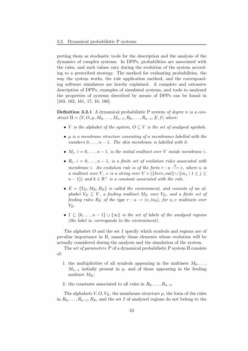
3.2. Dynamical probabilistic P systems
preting them as stochastic tools for the description and the analysis of thedynamics of complex systems. In DPPs, probabilities are associated withthe rules, and such values vary during the evolution of the system accord-ing to a prescribed strategy. The method for evaluating probabilities, theway the system works, the rule application method, and the correspond-ing software simulators are hereby explained. A complete and extensivedescription of DPPs, examples of simulated systems, and tools to analysedthe properties of systems described by means of DPPs can be found in[163, 162, 161, 17, 16, 160].
Definition 3.2.1 A dynamical probabilistic P system of degree n is a con-struct Π = (V,O, µ,M0, . . . ,Mn−1, R0, . . . , Rn−1, E, I) where:
• V is the alphabet of the system, O ⊆ V is the set of analysed symbols.
• µ is a membrane structure consisting of n membranes labelled with thenumbers 0, . . . , n − 1. The skin membrane is labelled with 0.
• Mi, i = 0, . . . , n− 1, is the initial multiset over V inside membrane i.
• Ri, i = 0, . . . , n − 1, is a finite set of evolution rules associated with
membrane i. An evolution rule is of the form r : uk
−→ v, where u isa multiset over V , v is a string over V × (here, out ∪ inj | 1 ≤ j ≤n − 1) and k ∈ R
+ is a constant associated with the rule.
• E = VE ,ME , RE is called the environment, and consists of an al-phabet VE ⊆ V , a feeding multiset ME over VE, and a finite set offeeding rules RE of the type r : u → (v, in0), for u, v multisets overVE.
• I ⊆ 0, . . . , n − 1 ∪ ∞ is the set of labels of the analysed regions(the label ∞ corresponds to the environment).
The alphabet O and the set I specify which symbols and regions are ofpeculiar importance in Π, namely those elements whose evolution will beactually considered during the analysis and the simulation of the system.
The set of parameters P of a dynamical probabilistic P system Π consistsof:
1. the multiplicities of all symbols appearing in the multisets M0, . . . ,Mn−1 initially present in µ, and of those appearing in the feedingmultiset ME ;
2. the constants associated to all rules in R0, . . . , Rn−1.
The alphabets V,O, VE , the membrane structure µ, the form of the rulesin R0, . . . , Rn−1, RE , and the set I of analysed regions do not belong to the
53
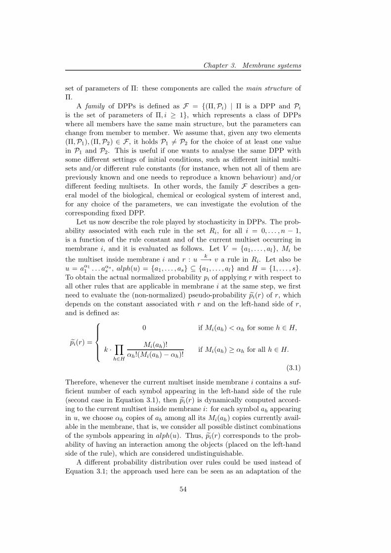
Chapter 3. Membrane systems
set of parameters of Π: these components are called the main structure ofΠ.
A family of DPPs is defined as F = (Π,Pi) | Π is a DPP and Pi
is the set of parameters of Π, i ≥ 1, which represents a class of DPPswhere all members have the same main structure, but the parameters canchange from member to member. We assume that, given any two elements(Π,P1), (Π,P2) ∈ F , it holds P1 6= P2 for the choice of at least one valuein P1 and P2. This is useful if one wants to analyse the same DPP withsome different settings of initial conditions, such as different initial multi-sets and/or different rule constants (for instance, when not all of them arepreviously known and one needs to reproduce a known behaviour) and/ordifferent feeding multisets. In other words, the family F describes a gen-eral model of the biological, chemical or ecological system of interest and,for any choice of the parameters, we can investigate the evolution of thecorresponding fixed DPP.
Let us now describe the role played by stochasticity in DPPs. The prob-ability associated with each rule in the set Ri, for all i = 0, . . . , n − 1,is a function of the rule constant and of the current multiset occurring inmembrane i, and it is evaluated as follows. Let V = a1, . . . , al, Mi be
the multiset inside membrane i and r : uk
−→ v a rule in Ri. Let also beu = aα1
1 . . . aαss , alph(u) = a1, . . . , as ⊆ a1, . . . , al and H = 1, . . . , s.
To obtain the actual normalized probability pi of applying r with respect toall other rules that are applicable in membrane i at the same step, we firstneed to evaluate the (non-normalized) pseudo-probability pi(r) of r, whichdepends on the constant associated with r and on the left-hand side of r,and is defined as:
pi(r) =
0 if Mi(ah) < αh for some h ∈ H,
k ·∏
h∈H
Mi(ah)!
αh!(Mi(ah) − αh)!if Mi(ah) ≥ αh for all h ∈ H.
(3.1)
Therefore, whenever the current multiset inside membrane i contains a suf-ficient number of each symbol appearing in the left-hand side of the rule(second case in Equation 3.1), then pi(r) is dynamically computed accord-ing to the current multiset inside membrane i: for each symbol ah appearingin u, we choose αh copies of ah among all its Mi(ah) copies currently avail-able in the membrane, that is, we consider all possible distinct combinationsof the symbols appearing in alph(u). Thus, pi(r) corresponds to the prob-ability of having an interaction among the objects (placed on the left-handside of the rule), which are considered undistinguishable.
A different probability distribution over rules could be used instead ofEquation 3.1; the approach used here can be seen as an adaptation of the
54
3.2. Dynamical probabilistic P systems
Stochastic Simulation Algorithm, introduced in [74], to include and preservethe maximal parallelism of rule application. Nonetheless, to the aim ofhaving the highest closeness to the biological system that one needs to model,other approaches could be investigated and compared as well. We also referto [19], for a method with real-valued reaction maps, and to [32], where somestochastic approaches for biological modelling are reviewed and compared.
Definition 3.2.2 An evolution rule is mute, if it is of the form u →(u, here), for some multiset u over V .
Mute rules, which do not change the current multiset in any way, canbe used as a trick to maintain the maximal parallelism at the level of ruleapplication, but not at the level of object consumption. In other words,assume to have a membrane with two rules a → (b, out), a → (c, here) anda multiset consisting of 10 copies of the symbol a. By using the maximalparallelism and the nondeterminism, in one step we would have α copies of cin the membrane, for some α ≥ 0, 10−α copies of b outside the membrane,and no more copies of a, since all occurrences had to be consumed. If themute rule a → (a, here) is added inside this membrane, then in one step –and still using the maximal parallelism and the nondeterminism – we wouldobtain α′ copies of c in the membrane, β copies of b outside the membrane,for some α′, β ≥ 0, and 10 − α′ − β copies of a in the membrane. So doing,not all occurrences of a are consumed (to be more precise, they are actuallyconsumed but also reproduced in the same form, in the same step), andthus the parallelism at the level of object consumption is no more maximal.Now, if we also associate stochastic constants to the rules, we can modulatethe reduced parallelism by intervening on (the value of) the constant of themute rule1.
When adding mute rules to a membrane, we do not want to change thedynamical conditions which are determined inside that membrane by theconstants associated to the other rules, and their respective mutual ratios.To this aim, we choose to apply the following strategy inside each membraneto compute the constant of any added mute rule, as well as the new constants
of its corresponding rules. Let S = r1 : uk1−→ v1, r2 : u
k2−→ v2, . . . , rh :
ukh−→ vh ⊆ Rj be a maximal subset of rules appearing inside a membrane
j and having the same left-hand side, for some u, v1, . . . , vh multisets overV , with vi 6= u for all i = 1, . . . , h, h ≥ 1. Let us also define KS =
∑hi=1 ki.
For any maximal set S of this type (with different sets having different left-
hand side multisets in the rules), we add the mute rule rh+1 : ukh+1−→ u
to S, and we call S′ = S ∪ rh+1. Since we want to preserve in S′ therelative dynamics of the rules initially present in S, we have to associate
1We remark that the analogous concept of tuning the “activity” of rules is also usedin the Metabolic Algorithm [19] with the name of transparent rules.
55
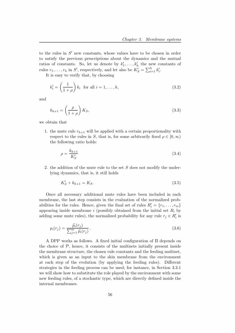
Chapter 3. Membrane systems
to the rules in S′ new constants, whose values have to be chosen in orderto satisfy the previous prescriptions about the dynamics and the mutualratios of constants. So, let us denote by k′
1, . . . , k′h the new constants of
rules r1, . . . , rh in S′, respectively, and let also be K ′S =
∑hi=1 k′
i.It is easy to verify that, by choosing
k′i =
(1
1 + ρ
)ki for all i = 1, . . . , h, (3.2)
and
kh+1 =
(ρ
1 + ρ
)KS , (3.3)
we obtain that
1. the mute rule rh+1 will be applied with a certain proportionality withrespect to the rules in S, that is, for some arbitrarily fixed ρ ∈ [0,∞)the following ratio holds:
ρ =kh+1
K ′S
(3.4)
2. the addition of the mute rule to the set S does not modify the under-lying dynamics, that is, it still holds
K ′S + kh+1 = KS . (3.5)
Once all necessary additional mute rules have been included in eachmembrane, the last step consists in the evaluation of the normalized prob-abilities for the rules. Hence, given the final set of rules R′
i = r1, . . . , rmappearing inside membrane i (possibly obtained from the initial set Ri byadding some mute rules), the normalized probability for any rule rj ∈ R′
i is
pi(rj) =pi(rj)∑m
j=1 pi(rj). (3.6)
A DPP works as follows. A fixed initial configuration of Π depends onthe choice of P, hence, it consists of the multisets initially present insidethe membrane structure, the chosen rule constants and the feeding multiset,which is given as an input to the skin membrane from the environmentat each step of the evolution (by applying the feeding rules). Differentstrategies in the feeding process can be used; for instance, in Section 3.3.1we will show how to substitute the role played by the environment with somenew feeding rules, of a stochastic type, which are directly defined inside theinternal membranes.
56
3.2. Dynamical probabilistic P systems
At each step of the evolution, all applicable rules are simultaneouslyapplied and all occurrences of the left-hand sides of the rules are consumed.We assume that the system evolves according to a universal clock (as in thebasic definition of P systems), that is, all membranes and the applicationof all rules are synchronized. The applied rules are chosen according tothe probability values dynamically assigned to them; clearly, the rules withthe highest normalized probability values will be more frequently tossed. Ifsome rules compete for objects and have the same probability value, thenobjects are nondeterministically assigned to them.
The simulation of the evolution of DPPs can be performed by meansof a software written in C language, which has been developed for singleprocessor PCs. In the simulations, the stochastic and parallel applicationof the rules is done by splitting each parallel step into several sequentialsub-steps. By exploiting the fact that the probability distribution and theapplicability of the rules are functions only of the left-hand side of the rulesand their constants, each single parallel step is separated into three stages:in the first one, the probabilities of rules are evaluated; in the second one,a random number generator is used to choose the rule to be applied andto correspondingly consume the objects appearing in its left-hand side; inthe third one, the multisets are updated using a stored trace of the rulespreviously tossed. Each stage starts only when the previous one has beenapplied to all the membranes in the DPP, and the same process is repeatedfor all evolution steps. A detailed description of the algorithm used for thesimulation of DPPs, and of its complexity, can be found in [162].
The simulations reported in Section 3.3.2 have been run using an imple-mentation of DPPs which exploit the MPI (Message Passing Interface) Clibraries in order to: (i) distribute the computation over a cluster of proces-sors to achieve scalability, (ii) have a direct mapping of the communicationsamong the membranes, and (iii) speed up the computation.
Using this “parallel” version of the simulator for DPPs, each membraneevolves independently from the others for everything but the communica-tion, such that it can reside on an independent MPI process. All the mem-branes of a DPP simultaneously evolve, and require to be synchronized atthe end of each step to allow the communication process. Since the rules areapplied in a maximal parallel way, in each membrane we can divide a stepinto three stages: (1) the computation of the probability distribution for therules, (2) the assignment to the rules of all objects which can be modifiedby rules, (3) the communication and multisets updating. Further details onthe MPI implementation of the DPPs simulation algorithm can be found in[32].
57
Chapter 3. Membrane systems
3.3 A DPP application: metapopulation systems
Metapopulations, also called multi-patch systems, are extensively investi-gated in Ecology to analyse the behaviour of interacting populations, to theaim of determining how a fragmented habitat influences local and globalpopulation persistence. A metapopulation consists of local populations, liv-ing in spatially separated habitat patches which can have different areas,quality or isolation, and a dispersal pool, which is the spatial place whereindividuals from a population spend some lifetime during the migrationamong patches. The dispersal of individuals is distance-dependent, it mayreduce the local population growth and lead to an increase in extinction riskdue also to environmental and demographical stochasticity, thus the persis-tence of populations is assumed to be balanced between local extinctionsand establishment of new populations in empty patches [85]. In multi-patchsystems, it is possible to distinguish between two principal classes of dynam-ics: the populations can locally interact inside a patch according to, e.g.,the Lotka-Volterra model of preys and predators [145], while the dispersalof individuals among patches can have effects on the global behaviour of thewhole system [93, 94, 191, 203].
The term “metapopulation” was introduced in [107], where a determin-istic model for population dynamics of insect pests in agriculture has beendeveloped. Lately, the topic has been largely applied to various populationsspecies in natural or artificial/theoretical fragmented habitat landscapes.Among the various modelling methods used so far to investigate metapopu-lation dynamics, we here recall stochastic patch occupancy models, populationviability analysis and spatially explicit population models.
Stochastic patch occupancy models (SPOMs) are based on the so-calledpresence/absence assumption, that is, they only model the occupancy stateof habitat patches, without considering any local population dynamics, andneither the populations sizes are requested. Discrete-time SPOMs are ho-mogeneous first-order Markov chains in which the occupancy pattern at anytime t + 1 depends only on the pattern at time t; as a consequence, thesemodels are well applied to organisms which have one generation per year,such as insects. Recently, a software for SPOMs, namely SPOMSIM, hasalso been developed for the automatic inclusion and analysis of several pa-rameters and features (see [136]).
Population viability analysis (PVA) models are used in conservationassessment issues, well applied to single-species (e.g., rare or threatenedspecies) populations analysis with respect to their risk – or expected time– of extinction, or their chance of recovery, thus measuring the viabilityrequirements of the species and how likely it is for that species to persistalong a certain future time. The reliability of these models and the pa-rameter estimation are usually based on a large set of demographic, habitatand individual-based data, specific for the species under investigation. PVA
58
3.3. A DPP application: metapopulation systems
methods usually address aspects of management, such as impact of humanactivities, responses of species to reintroduction, captive breeding or naturereserves, and more. For additional information about this methodology andalternative ones for conservation assessment studies, see [2].
Spatially explicit population models (SEPMs) are individual-based orpopulation-based models, that combine a simulator for the populations witha map of the landscape, such that landscape features can be explicitly in-corporated into the model, to analyse how population dynamics is affectedby any change in landscape (e.g., climate change, regional land-use, impactof fire or other global phenomena). Complex real-world landscape and theresponse of population to habitat changes can thus be investigated withinthese models. SEPMs require to know life history, demographic informa-tion and several habitat-specific data about the behaviours of dispersal andhabitat-selection of the studied populations. Temporal or spatial variationof the landscape can also be incorporated, thus creating dynamical land-scape where the distribution of suitable and unsuitable patches changes intime. Sensitivity analysis can be used within SEPMs for the estimation ofparameters which are not available from ecological studies, e.g., for habitatselection or for dispersal behaviours, and to gain insights about the optimaland adaptive management strategies in varying contexts [40]. For furthernotions about SEPMs we refer to the review work by [52].
Whichever the modelling method is chosen for analysing a peculiar (e-mergent) behaviour of interacting populations in fragmented habitat, spe-cific properties of the system can be, or even have to be, explicitly or implic-itly considered, as the ones that we remark in the following (see [85, 136, 86]for further details).
Referring to the landscape, most models take care of the spatial struc-ture, the local environmental quality, the patch area and connectivity (iso-lation), to grasp the effect of habitat fragmentation on species persistence,since high connectivity decreases local extinction risk (this is called the “res-cue effect”) and local conditions determines the growth and survival of patchpopulations. Moreover, dispersal and colonization are distance-dependentelements which give meaning to landscape structure in a spatial model. Asfor population interactions and dynamics, colonization can be related or notto cooperation of immigrating individuals (in the first case, it is called “Alleeeffect”). Within-patch dynamics is claimed to improve the understandingof natural systems; models which do not take care of it, thus only assumingwhether a patch is occupied or not, usually consider local dynamics on afaster time scale with respect to the global dynamics, and also neglect thedependence of colonization and extinction rates on population sizes. Finally,regional stochasticity takes care of “bad” or “good” years over the local en-vironmental quality. As we will explain later on, some of these issues will beexplicitly considered in the next section for defining the membrane systemmodel for metapopulations.
59
Chapter 3. Membrane systems
In what follows, we define a model of metapopulations with predator-prey dynamics by means of DPPs, where additional features are used inorder to catch and better describe relevant properties of the modelled sys-tem. Namely, we will use a membrane structure of a novel type, wherethe spatial arrangement and the dimension of regions matter. With thischoice we can give a proper description of a real (or artificial laboratory)landscape, and thus correctly analyse the dynamics of species interactions,via the definition of appropriate rule constants related to the fixed geom-etry. We then apply the generic model to some test case studies, and weinvestigate some emergent metapopulation behaviours, such as the effects ofstochastic breeding, migration and colonization, isolation of patches, etc.
3.3.1 The modelling framework
Let µ be a membrane structure with degree n+1 and depth 2, with the skinmembrane labelled with 0 and the internal membranes labelled with num-bers 1, . . . , n. In the following, we will refer without distinction to the skinmembrane or the dispersal pool, and to the internal membranes or regionsor patches. For the modelling of a metapopulation, the membrane structurehas to be intended as a set of spatially distributed regions, each one com-pleted with a “size”, which represent the area of the 2-dimensional patch,and with a fixed “distance” with respect to all other regions. Since themembrane structure is assumed to have here a precise spatial arrangement,we will not represent it as a string of well-matching square brackets where,as usual, any permutation of internal membranes would give rise to topo-logically equivalent structures (which is something that we want to avoid).Instead, to describe the set of internal membranes, we will use an undirectedweighted graph with node attributes, thus outlining both the spatial distri-bution of patches and the relevant additional features associated to them:the area of a patch is needed to define the density of the populations livinginside the patch (and thus to provide a better description of the dynamics),while the distance is needed to identify isolated patches, as well as to definethe dispersal rates inside the pool. The distance among patches is not tobe necessarily intended as a physical measure of how far a patch is fromanother one, but it can also represent a measure of how hard it is to movefrom one patch to another one due to, e.g., the geographical morphology ofthe landscape (presence of mountain chains, deep rivers or sea among thepatches) or to other general local conditions (zones in the pool which causehigh risks for survival). Hence, we will more generally call this distance thecost.
We also remark that, for metapopulation models, each region has to beconsidered as part of a 2-dimensional space, and not as a closed surface ina 3-dimensional space as it is usually implicit in P systems.
The membrane structure, the areas and the patch mutual costs are as-
60
3.3. A DPP application: metapopulation systems
sumed to be fixed in the model we propose here. The modification of theseelements could be forced, and would indeed be necessary, in the analysis oflandscapes whose main structure changes during time, such as patches dis-appearing or reducing their dimension (e.g., a fire burning a forest), patchesincreasing their dimension (e.g., new borders built around a protected park),or even patches in different positions in the pool (e.g., in laboratory experi-ments where patches are glass boxes that can be freely moved around).
Formally, to associate a spatial structure to the membrane structure, wedefine a weighted undirected graph G = (N∆, E,w) where:
• N∆ is the set of nodes, or vertices, such that, to each node x ∈ N∆,there is associated a value a ∈ ∆, being ∆ a set of attributes of somekind;
• E ⊆ (x, y) | x, y ∈ N∆ is the set of (undirected) edges betweennodes;
• w : E → R+ is the weight function associating a cost to each edge.
In our case, the set of nodes N∆ coincides with the set m1, . . . ,mnof internal membranes, the attribute of a patch represents the area of thepatch, the edges characterize which patch is directly reachable from anyother patch (self-edges of the type (mi,mi) might exist as well), and theweight wi,j of an edge (mi,mj) represent a cost to measure the effort thatindividuals have to face when moving from patch mi to mj through thedispersal pool.
Note that, if a patch mi is directly reachable from patch mj, then theindividuals exiting from patch mi will (possibly) enter patch mj after sometime spent in the pool (and vice versa), thus we are not interested in findingwhether there exists a path in the graph such that individuals exiting frommi will enter and leave other patches in the graph path before finally arriv-ing in mj. Self-edges obviously represent the possible action of individualsexiting a patch and then entering it again. Moreover, we consider the caseof undirected graphs, though also directed graphs with two possibly edgesbetween any couple of patches can be used, and their relative costs can bedifferent, thus better characterizing the landscape nature (e.g., the cost ofclimbing a mountain can be different from the cost of descending from it).
The area of a patch mi, i = 1, . . . , n, is a value σi ∈ R+. We will not
define the area of the pool, we implicitly assume that it is large enoughto contain all patches and to allow the dispersal of individuals, that is,σ0 ≫
∑ni=1 σi.
Definition 3.3.1 Let V be the alphabet of population species. The densityof patch mi, i = 0, 1, . . . , n, with respect to population species X ∈ V , is
δX(mi) =|X|mi
σi, (3.7)
61
Chapter 3. Membrane systems
where |X|midenotes the number of individuals of species X inside patch mi.
The total density of patch mi with respect to all population species is definedas
δV (mi) =1
σi
∑
X∈V
|X|mi. (3.8)
Definition 3.3.2 The mean cost of the graph G associated to the membranestructure µ is the value
wG =
∑ni,j=1 wi,j
∑n−1k=1 n − k
. (3.9)
Definition 3.3.3 A patch mi, for some i = 1, . . . , n, is said to be isolatedif wi,j ≫ wG, for all j = 1, . . . , n.
In other words, a patch can be considered isolated if its distance from anyother patch is very high, or if the cost to reach it (or to reach another patchwhen migrating from it) is much higher than the mean cost for reaching anyother patch. As a consequence, the probability of the population individualsmigrating from, or moving to, an isolated patch will be accordingly defined,in order to capture this characteristic of metapopulations.
Given all the necessary definitions, we can now introduce our DPP modelΠ for a generic metapopulation consisting on n patches, a dispersal pool,and two population species, one for preys and one for predators. We willassume that the populations dynamics inside each patch follows the Lotka-Volterra model (see [162] for a previous description with DPPs) and that,without loosing in generality, the sustenance resources are identical for allspecies. Hence, let
Π = (V,O, µ, I,G,M0 , . . . ,Mn, R0, . . . , Rn)
be such that
• V = A,A′,X, Y, Y1, . . . , Yn consists of the symbol A for sustenanceresources, X for the species of preys, Y for the species of predators. A′
is used to simulate the stochastic feeding of resources, while Y1, . . . , Yn
are used for denoting, via the subscripts 1, . . . , n, which is the origi-nating patch of the predators occurring in the pool, as it will be clearbelow.
• O = X,Y is the set of analysed symbols.
• µ is a membrane structure with n elementary membranes, each cor-responding to a patch in the metapopulation system. The skin mem-brane plays the role of the dispersal pool.
62
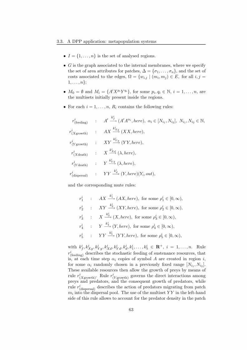
3.3. A DPP application: metapopulation systems
• I = 1, . . . , n is the set of analysed regions.
• G is the graph associated to the internal membranes, where we specifythe set of area attributes for patches, ∆ = σ1, . . . , σn, and the set ofcosts associated to the edges, Ω = wi,j | (mi,mj) ∈ E, for all i, j =1, . . . , n;
• M0 = ∅ and Mi = A′XpiY qi, for some pi, qi ∈ N, i = 1, . . . , n, arethe multisets initially present inside the regions.
• For each i = 1, . . . , n, Ri contains the following rules:
ri(feeding) : A′
kif
−→ (A′Aαi , here), αi ∈ [Ni1 , Ni2 ], Ni1, Ni2 ∈ N,
ri(Xgrowth) : AX
kiXg
−→ (XX,here),
ri(Y growth) : XY
kiY g
−→ (Y Y, here),
ri(Xdeath) : X
kiXd−→ (λ, here),
ri(Y death) : Y
kiY d−→ (λ, here),
ri(dispersal) : Y Y
kid−→ (Y, here)(Yi, out),
and the corresponding mute rules:
ri1 : AX
ki1−→ (AX,here), for some ρi
1 ∈ [0,∞),
ri2 : XY
ki2−→ (XY, here), for some ρi
2 ∈ [0,∞),
ri3 : X
ki3−→ (X,here), for some ρi
3 ∈ [0,∞),
ri4 : Y
ki4−→ (Y, here), for some ρi
4 ∈ [0,∞),
ri5 : Y Y
ki5−→ (Y Y, here), for some ρi
5 ∈ [0,∞),
with kif , ki
Xg, kiY g, k
iXd, k
iY d, k
id, k
i1, . . . , k
i5 ∈ R+, i = 1, . . . , n. Rule
ri(feeding) describes the stochastic feeding of sustenance resources, that
is, at each time step αi copies of symbol A are created in region i,for some αi randomly chosen in a previously fixed range [Ni1 , Ni2 ].These available resources then allow the growth of preys by means ofrule ri
(Xgrowth). Rule ri(Y growth) governs the direct interactions among
preys and predators, and the consequent growth of predators, whilerule ri
(dispersal) describes the action of predators migrating from patchmi into the dispersal pool. The use of the multiset Y Y in the left-handside of this rule allows to account for the predator density in the patch
63
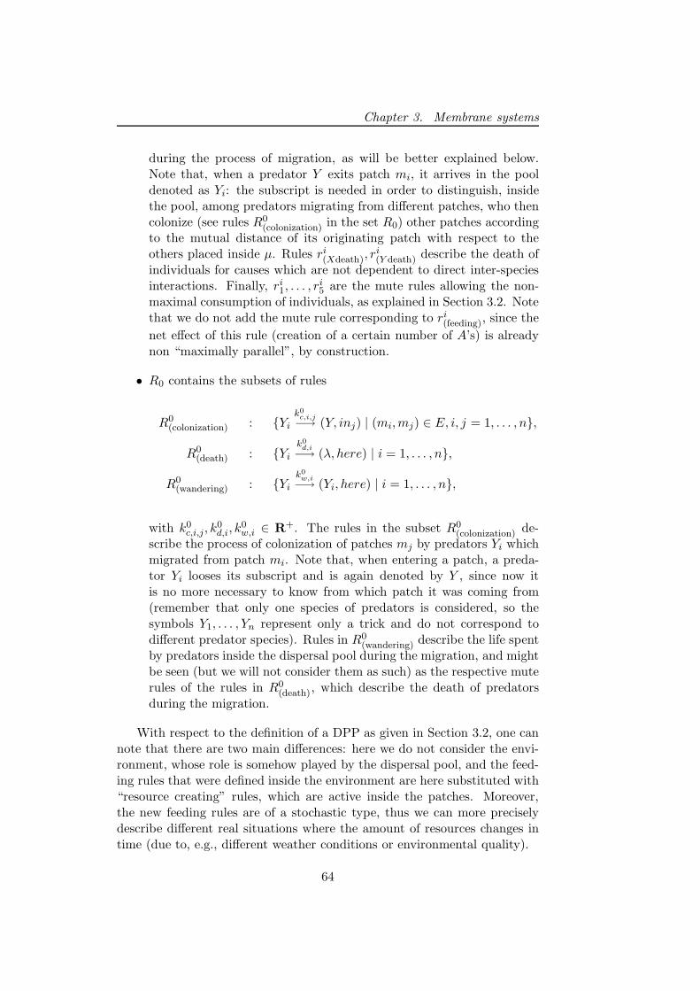
Chapter 3. Membrane systems
during the process of migration, as will be better explained below.Note that, when a predator Y exits patch mi, it arrives in the pooldenoted as Yi: the subscript is needed in order to distinguish, insidethe pool, among predators migrating from different patches, who thencolonize (see rules R0
(colonization) in the set R0) other patches accordingto the mutual distance of its originating patch with respect to theothers placed inside µ. Rules ri
(Xdeath), ri(Y death) describe the death of
individuals for causes which are not dependent to direct inter-speciesinteractions. Finally, ri
1, . . . , ri5 are the mute rules allowing the non-
maximal consumption of individuals, as explained in Section 3.2. Notethat we do not add the mute rule corresponding to ri
(feeding), since the
net effect of this rule (creation of a certain number of A’s) is alreadynon “maximally parallel”, by construction.
• R0 contains the subsets of rules
R0(colonization) : Yi
k0c,i,j−→ (Y, inj) | (mi,mj) ∈ E, i, j = 1, . . . , n,
R0(death) : Yi
k0d,i
−→ (λ, here) | i = 1, . . . , n,
R0(wandering) : Yi
k0w,i
−→ (Yi, here) | i = 1, . . . , n,
with k0c,i,j, k
0d,i, k
0w,i ∈ R+. The rules in the subset R0
(colonization) de-scribe the process of colonization of patches mj by predators Yi whichmigrated from patch mi. Note that, when entering a patch, a preda-tor Yi looses its subscript and is again denoted by Y , since now itis no more necessary to know from which patch it was coming from(remember that only one species of predators is considered, so thesymbols Y1, . . . , Yn represent only a trick and do not correspond todifferent predator species). Rules in R0
(wandering) describe the life spentby predators inside the dispersal pool during the migration, and mightbe seen (but we will not consider them as such) as the respective muterules of the rules in R0
(death), which describe the death of predatorsduring the migration.
With respect to the definition of a DPP as given in Section 3.2, one cannote that there are two main differences: here we do not consider the envi-ronment, whose role is somehow played by the dispersal pool, and the feed-ing rules that were defined inside the environment are here substituted with“resource creating” rules, which are active inside the patches. Moreover,the new feeding rules are of a stochastic type, thus we can more preciselydescribe different real situations where the amount of resources changes intime (due to, e.g., different weather conditions or environmental quality).
64
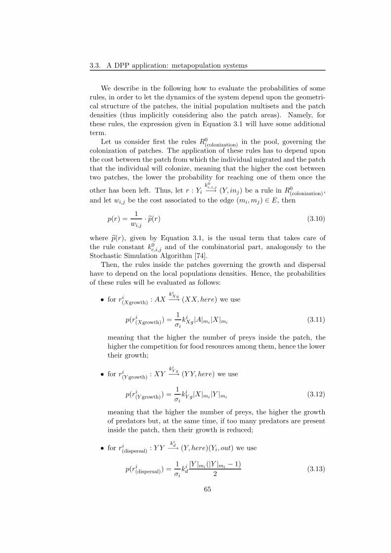
3.3. A DPP application: metapopulation systems
We describe in the following how to evaluate the probabilities of somerules, in order to let the dynamics of the system depend upon the geometri-cal structure of the patches, the initial population multisets and the patchdensities (thus implicitly considering also the patch areas). Namely, forthese rules, the expression given in Equation 3.1 will have some additionalterm.
Let us consider first the rules R0(colonization) in the pool, governing the
colonization of patches. The application of these rules has to depend uponthe cost between the patch from which the individual migrated and the patchthat the individual will colonize, meaning that the higher the cost betweentwo patches, the lower the probability for reaching one of them once the
other has been left. Thus, let r : Yi
k0c,i,j−→ (Y, inj) be a rule in R0
(colonization),
and let wi,j be the cost associated to the edge (mi,mj) ∈ E, then
p(r) =1
wi,j· p(r) (3.10)
where p(r), given by Equation 3.1, is the usual term that takes care ofthe rule constant k0
c,i,j and of the combinatorial part, analogously to theStochastic Simulation Algorithm [74].
Then, the rules inside the patches governing the growth and dispersalhave to depend on the local populations densities. Hence, the probabilitiesof these rules will be evaluated as follows:
• for ri(Xgrowth) : AX
kiXg
−→ (XX,here) we use
p(ri(Xgrowth)) =
1
σiki
Xg|A|mi|X|mi
(3.11)
meaning that the higher the number of preys inside the patch, thehigher the competition for food resources among them, hence the lowertheir growth;
• for ri(Y growth) : XY
kiY g
−→ (Y Y, here) we use
p(ri(Y growth)) =
1
σiki
Y g|X|mi|Y |mi
(3.12)
meaning that the higher the number of preys, the higher the growthof predators but, at the same time, if too many predators are presentinside the patch, then their growth is reduced;
• for ri(dispersal) : Y Y
kid−→ (Y, here)(Yi, out) we use
p(ri(dispersal)) =
1
σiki
d
|Y |mi(|Y |mi
− 1)
2(3.13)
65
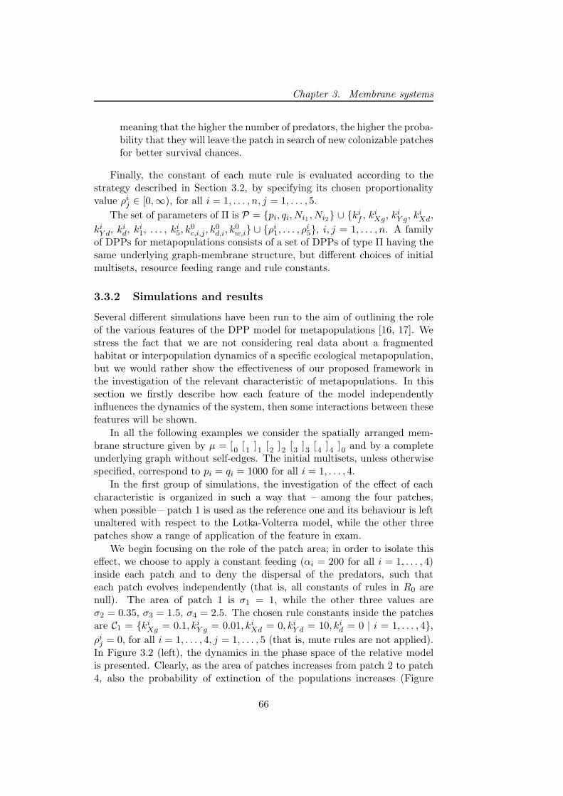
Chapter 3. Membrane systems
meaning that the higher the number of predators, the higher the proba-bility that they will leave the patch in search of new colonizable patchesfor better survival chances.
Finally, the constant of each mute rule is evaluated according to thestrategy described in Section 3.2, by specifying its chosen proportionalityvalue ρi
j ∈ [0,∞), for all i = 1, . . . , n, j = 1, . . . , 5.
The set of parameters of Π is P = pi, qi, Ni1 , Ni2 ∪ kif , ki
Xg, kiY g, ki
Xd,
kiY d, ki
d, ki1, . . . , ki
5, k0c,i,j, k
0d,i, k
0w,i ∪ ρi
1, . . . , ρi5, i, j = 1, . . . , n. A family
of DPPs for metapopulations consists of a set of DPPs of type Π having thesame underlying graph-membrane structure, but different choices of initialmultisets, resource feeding range and rule constants.
3.3.2 Simulations and results
Several different simulations have been run to the aim of outlining the roleof the various features of the DPP model for metapopulations [16, 17]. Westress the fact that we are not considering real data about a fragmentedhabitat or interpopulation dynamics of a specific ecological metapopulation,but we would rather show the effectiveness of our proposed framework inthe investigation of the relevant characteristic of metapopulations. In thissection we firstly describe how each feature of the model independentlyinfluences the dynamics of the system, then some interactions between thesefeatures will be shown.
In all the following examples we consider the spatially arranged mem-brane structure given by µ = [0 [1 ]1 [2 ]2 [3 ]3 [4 ]4 ]0 and by a completeunderlying graph without self-edges. The initial multisets, unless otherwisespecified, correspond to pi = qi = 1000 for all i = 1, . . . , 4.
In the first group of simulations, the investigation of the effect of eachcharacteristic is organized in such a way that – among the four patches,when possible – patch 1 is used as the reference one and its behaviour is leftunaltered with respect to the Lotka-Volterra model, while the other threepatches show a range of application of the feature in exam.
We begin focusing on the role of the patch area; in order to isolate thiseffect, we choose to apply a constant feeding (αi = 200 for all i = 1, . . . , 4)inside each patch and to deny the dispersal of the predators, such thateach patch evolves independently (that is, all constants of rules in R0 arenull). The area of patch 1 is σ1 = 1, while the other three values areσ2 = 0.35, σ3 = 1.5, σ4 = 2.5. The chosen rule constants inside the patchesare C1 = ki
Xg = 0.1, kiY g = 0.01, ki
Xd = 0, kiY d = 10, ki
d = 0 | i = 1, . . . , 4,
ρij = 0, for all i = 1, . . . , 4, j = 1, . . . , 5 (that is, mute rules are not applied).
In Figure 3.2 (left), the dynamics in the phase space of the relative modelis presented. Clearly, as the area of patches increases from patch 2 to patch4, also the probability of extinction of the populations increases (Figure
66
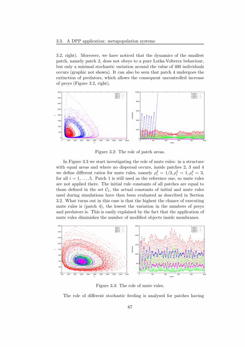
3.3. A DPP application: metapopulation systems
3.2, right). Moreover, we have noticed that the dynamics of the smallestpatch, namely patch 2, does not obeys to a pure Lotka-Volterra behaviour,but only a minimal stochastic variation around the value of 400 individualsoccurs (graphic not shown). It can also be seen that patch 4 undergoes theextinction of predators, which allows the consequent uncontrolled increaseof preys (Figure 3.2, right).
0
500
1000
1500
2000
2500
3000
3500
4000
0 1000 2000 3000 4000 5000 6000 7000 8000 9000 10000
Y
X
patch 1patch 3patch 4patch 2
0
2000
4000
6000
8000
10000
0 200 400 600 800 1000
Indi
vidu
als
Steps
X patch 1Y patch 1X patch 4Y patch 4
Figure 3.2: The role of patch areas.
In Figure 3.3 we start investigating the role of mute rules: in a structurewith equal areas and where no dispersal occurs, inside patches 2, 3 and 4we define different ratios for mute rules, namely ρ2
i = 1/3, ρ3i = 1, ρ4
i = 3,for all i = 1, . . . , 5. Patch 1 is still used as the reference one, so mute rulesare not applied there. The initial rule constants of all patches are equal tothose defined in the set C1, the actual constants of initial and mute rulesused during simulations have then been evaluated as described in Section3.2. What turns out in this case is that the highest the chance of executingmute rules is (patch 4), the lowest the variation in the numbers of preysand predators is. This is easily explained by the fact that the application ofmute rules diminishes the number of modified objects inside membranes.
0
200
400
600
800
1000
1200
1400
1600
400 600 800 1000 1200 1400 1600 1800 2000 2200 2400
Y
X
patch 1patch 2patch 3patch 4
0
500
1000
1500
2000
2500
0 200 400 600 800 1000
Indi
vidu
als
Steps
X patch 1Y patch 1X patch 3Y patch 3
Figure 3.3: The role of mute rules.
The role of different stochastic feeding is analysed for patches having
67
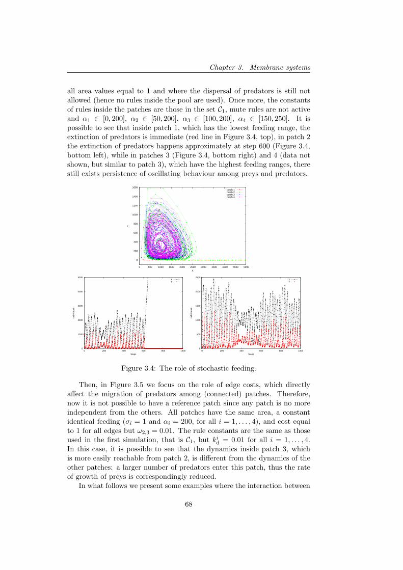
Chapter 3. Membrane systems
all area values equal to 1 and where the dispersal of predators is still notallowed (hence no rules inside the pool are used). Once more, the constantsof rules inside the patches are those in the set C1, mute rules are not activeand α1 ∈ [0, 200], α2 ∈ [50, 200], α3 ∈ [100, 200], α4 ∈ [150, 250]. It ispossible to see that inside patch 1, which has the lowest feeding range, theextinction of predators is immediate (red line in Figure 3.4, top), in patch 2the extinction of predators happens approximately at step 600 (Figure 3.4,bottom left), while in patches 3 (Figure 3.4, bottom right) and 4 (data notshown, but similar to patch 3), which have the highest feeding ranges, therestill exists persistence of oscillating behaviour among preys and predators.
0
200
400
600
800
1000
1200
1400
1600
0 500 1000 1500 2000 2500 3000 3500 4000 4500 5000
Y
X
patch 1patch 2patch 3patch 4
0
1000
2000
3000
4000
5000
0 200 400 600 800 1000
Indi
vidu
als
Steps
XY
0
500
1000
1500
2000
2500
0 200 400 600 800 1000
Indi
vidu
als
Steps
XY
Figure 3.4: The role of stochastic feeding.
Then, in Figure 3.5 we focus on the role of edge costs, which directlyaffect the migration of predators among (connected) patches. Therefore,now it is not possible to have a reference patch since any patch is no moreindependent from the others. All patches have the same area, a constantidentical feeding (σi = 1 and αi = 200, for all i = 1, . . . , 4), and cost equalto 1 for all edges but ω2,3 = 0.01. The rule constants are the same as thoseused in the first simulation, that is C1, but ki
d = 0.01 for all i = 1, . . . , 4.In this case, it is possible to see that the dynamics inside patch 3, whichis more easily reachable from patch 2, is different from the dynamics of theother patches: a larger number of predators enter this patch, thus the rateof growth of preys is correspondingly reduced.
In what follows we present some examples where the interaction between
68
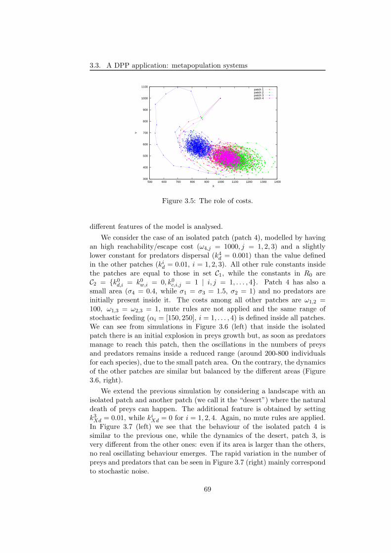
3.3. A DPP application: metapopulation systems
300
400
500
600
700
800
900
1000
1100
500 600 700 800 900 1000 1100 1200 1300 1400
Y
X
patch 1patch 2patch 3patch 4
Figure 3.5: The role of costs.
different features of the model is analysed.
We consider the case of an isolated patch (patch 4), modelled by havingan high reachability/escape cost (ω4,j = 1000, j = 1, 2, 3) and a slightlylower constant for predators dispersal (k4
d = 0.001) than the value definedin the other patches (ki
d = 0.01, i = 1, 2, 3). All other rule constants insidethe patches are equal to those in set C1, while the constants in R0 areC2 = k0
d,i = k0w,i = 0, k0
c,i,j = 1 | i, j = 1, . . . , 4. Patch 4 has also asmall area (σ4 = 0.4, while σ1 = σ3 = 1.5, σ2 = 1) and no predators areinitially present inside it. The costs among all other patches are ω1,2 =100, ω1,3 = ω2,3 = 1, mute rules are not applied and the same range ofstochastic feeding (αi = [150, 250], i = 1, . . . , 4) is defined inside all patches.We can see from simulations in Figure 3.6 (left) that inside the isolatedpatch there is an initial explosion in preys growth but, as soon as predatorsmanage to reach this patch, then the oscillations in the numbers of preysand predators remains inside a reduced range (around 200-800 individualsfor each species), due to the small patch area. On the contrary, the dynamicsof the other patches are similar but balanced by the different areas (Figure3.6, right).
We extend the previous simulation by considering a landscape with anisolated patch and another patch (we call it the “desert”) where the naturaldeath of preys can happen. The additional feature is obtained by settingk3
Xd = 0.01, while kiXd = 0 for i = 1, 2, 4. Again, no mute rules are applied.
In Figure 3.7 (left) we see that the behaviour of the isolated patch 4 issimilar to the previous one, while the dynamics of the desert, patch 3, isvery different from the other ones: even if its area is larger than the others,no real oscillating behaviour emerges. The rapid variation in the number ofpreys and predators that can be seen in Figure 3.7 (right) mainly correspondto stochastic noise.
69
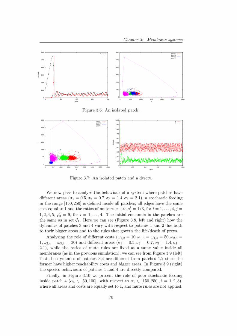
Chapter 3. Membrane systems
0
1000
2000
3000
4000
5000
6000
0 50 100 150 200
Indi
vidu
als
Steps
XY
0
1000
2000
3000
4000
5000
6000
0 1000 2000 3000 4000 5000 6000
Y
X
patch 1patch 2patch 3patch 4
Figure 3.6: An isolated patch.
0
500
1000
1500
2000
2500
3000
0 500 1000 1500 2000 2500 3000 3500 4000
Y
X
patch 1patch 2patch 3patch 4
0
100
200
300
400
500
600
700
800
900
1000
0 200 400 600 800 1000
Indi
vidu
als
Steps
XY
Figure 3.7: An isolated patch and a desert.
We now pass to analyse the behaviour of a system where patches havedifferent areas (σ1 = 0.5, σ2 = 0.7, σ3 = 1.4, σ4 = 2.1), a stochastic feedingin the range [150, 250] is defined inside all patches, all edges have the samecost equal to 1 and the ratios of mute rules are ρi
j = 1/3, for i = 1, . . . , 4, j =
1, 2, 4, 5, ρi3 = 9, for i = 1, . . . , 4. The initial constants in the patches are
the same as in set C1. Here we can see (Figure 3.8, left and right) how thedynamics of patches 3 and 4 vary with respect to patches 1 and 2 due bothto their bigger areas and to the rules that govern the life/death of preys.
Analysing the role of different costs (ω1,2 = 10, ω1,3 = ω1,4 = 50, ω2,3 =1, ω2,4 = ω3,4 = 30) and different areas (σ1 = 0.5, σ2 = 0.7, σ3 = 1.4, σ4 =2.1), while the ratios of mute rules are fixed at a same value inside allmembranes (as in the previous simulation), we can see from Figure 3.9 (left)that the dynamics of patches 3,4 are different from patches 1,2 since theformer have higher reachability costs and bigger areas. In Figure 3.9 (right)the species behaviours of patches 1 and 4 are directly compared.
Finally, in Figure 3.10 we present the role of poor stochastic feedinginside patch 4 (α4 ∈ [50, 100], with respect to αi ∈ [150, 250], i = 1, 2, 3),where all areas and costs are equally set to 1, and mute rules are not applied.
70
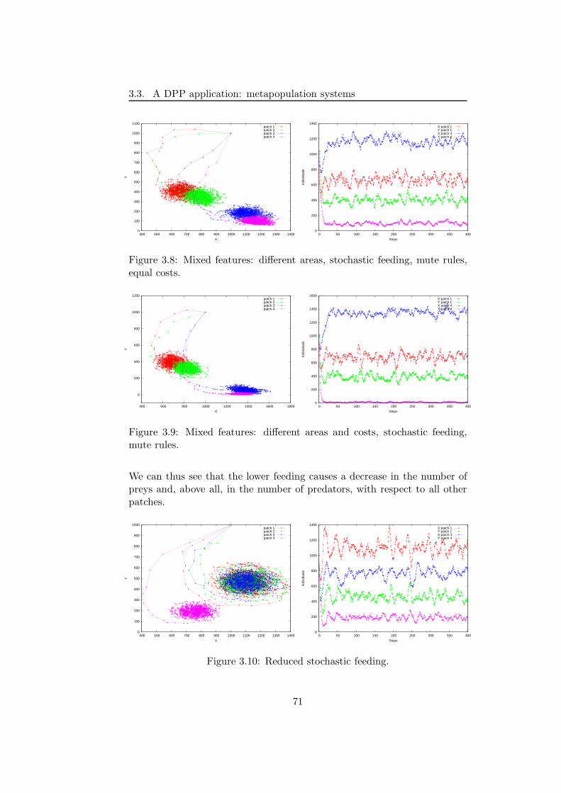
3.3. A DPP application: metapopulation systems
0
100
200
300
400
500
600
700
800
900
1000
1100
400 500 600 700 800 900 1000 1100 1200 1300 1400
Y
X
patch 1patch 2patch 3patch 4
0
200
400
600
800
1000
1200
1400
0 50 100 150 200 250 300 350 400
Indi
vidu
als
Steps
X patch 1Y patch 1X patch 4Y patch 4
Figure 3.8: Mixed features: different areas, stochastic feeding, mute rules,equal costs.
0
200
400
600
800
1000
1200
400 600 800 1000 1200 1400 1600 1800
Y
X
patch 1patch 2patch 3patch 4
0
200
400
600
800
1000
1200
1400
1600
0 50 100 150 200 250 300 350 400
Indi
vidu
als
Steps
X patch 1Y patch 1X patch 4Y patch 4
Figure 3.9: Mixed features: different areas and costs, stochastic feeding,mute rules.
We can thus see that the lower feeding causes a decrease in the number ofpreys and, above all, in the number of predators, with respect to all otherpatches.
0
100
200
300
400
500
600
700
800
900
1000
400 500 600 700 800 900 1000 1100 1200 1300 1400
Y
X
patch 1patch 2patch 3patch 4
0
200
400
600
800
1000
1200
1400
0 50 100 150 200 250 300 350 400
Indi
vidu
als
Steps
X patch 1Y patch 1X patch 4Y patch 4
Figure 3.10: Reduced stochastic feeding.
71
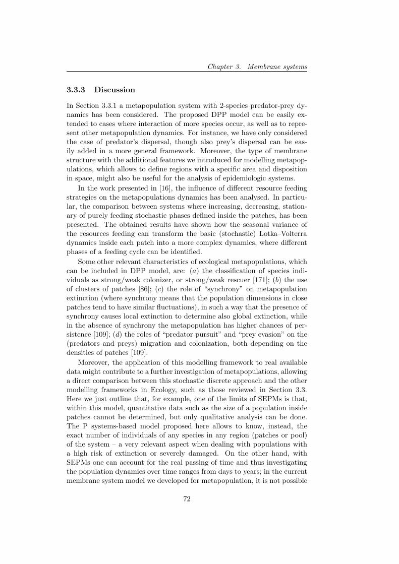
Chapter 3. Membrane systems
3.3.3 Discussion
In Section 3.3.1 a metapopulation system with 2-species predator-prey dy-namics has been considered. The proposed DPP model can be easily ex-tended to cases where interaction of more species occur, as well as to repre-sent other metapopulation dynamics. For instance, we have only consideredthe case of predator’s dispersal, though also prey’s dispersal can be eas-ily added in a more general framework. Moreover, the type of membranestructure with the additional features we introduced for modelling metapop-ulations, which allows to define regions with a specific area and dispositionin space, might also be useful for the analysis of epidemiologic systems.
In the work presented in [16], the influence of different resource feedingstrategies on the metapopulations dynamics has been analysed. In particu-lar, the comparison between systems where increasing, decreasing, station-ary of purely feeding stochastic phases defined inside the patches, has beenpresented. The obtained results have shown how the seasonal variance ofthe resources feeding can transform the basic (stochastic) Lotka–Volterradynamics inside each patch into a more complex dynamics, where differentphases of a feeding cycle can be identified.
Some other relevant characteristics of ecological metapopulations, whichcan be included in DPP model, are: (a) the classification of species indi-viduals as strong/weak colonizer, or strong/weak rescuer [171]; (b) the useof clusters of patches [86]; (c) the role of “synchrony” on metapopulationextinction (where synchrony means that the population dimensions in closepatches tend to have similar fluctuations), in such a way that the presence ofsynchrony causes local extinction to determine also global extinction, whilein the absence of synchrony the metapopulation has higher chances of per-sistence [109]; (d) the roles of “predator pursuit” and “prey evasion” on the(predators and preys) migration and colonization, both depending on thedensities of patches [109].
Moreover, the application of this modelling framework to real availabledata might contribute to a further investigation of metapopulations, allowinga direct comparison between this stochastic discrete approach and the othermodelling frameworks in Ecology, such as those reviewed in Section 3.3.Here we just outline that, for example, one of the limits of SEPMs is that,within this model, quantitative data such as the size of a population insidepatches cannot be determined, but only qualitative analysis can be done.The P systems-based model proposed here allows to know, instead, theexact number of individuals of any species in any region (patches or pool)of the system – a very relevant aspect when dealing with populations witha high risk of extinction or severely damaged. On the other hand, withSEPMs one can account for the real passing of time and thus investigatingthe population dynamics over time ranges from days to years; in the currentmembrane system model we developed for metapopulation, it is not possible
72

3.3. A DPP application: metapopulation systems
to include such feature yet, though accounting for real evolution time is ahot topic in P systems and already a work in progress [30, 20].
73

Chapter 3. Membrane systems
74
Chapter 4
τ–DPP
In this chapter, a novel algorithm for the simulation of chemical and biolog-ical systems composed by many volumes will be described. This approach,called τ–DPP, has been first presented in [30]; it combines some features ofmembrane systems, in particular of the DPP variant (see Section 3.2) withthe simulation strategy used in the tau-leaping algorithm (see Section 1.3).τ -DPP exploits a particular kind of reactions, called communication rules,to move objects between volumes, rather than considering diffusive processes(as, for instance, in the NSM [57] and in the Bτ -SSSA [117]). Therefore,both “classic” reactions and communication rules will be selected using thesame strategy.
τ -DPP has been introduced to the aim of extending the single-volumealgorithm of tau-leaping [26], in order to handle multi-volume systems wheredistinct volumes are arranged according to a specified hierarchy, and withthe additional assumption that the topological structure and the size of thevolumes do not change during the system evolution. As already seen inChapter 3, this condition is well satisfied by the membrane structure of a Psystem, which is also the underlying spatial arrangement used within τ -DPP.Indeed, τ -DPP presents a close correspondence to DPP, but the first allowsa quantitative description of the system’s dynamics, while in the second theobtained behaviour is only qualitative.
In order to correctly describe the behaviour of a system, τ -DPP runs inparallel inside each volume. A modified version of the tau-leaping proce-dure presented in [26] is exploited for the computation of the length of thestep τ . In this novel version of the simulation algorithm, the least value forthe time increment, among those computed inside each volume, is used tosample the number of reactions to execute (as in the original tau-leaping al-gorithm). Thanks to this “common” time increment, shared by all volumes,the simulation is synchronized at each step, allowing the correct passage ofthe molecules involved in communication rules.
The computational cost of the τ -DPP algorithm is the same as the tau-
75
Chapter 4. τ–DPP
leaping strategy, for a single volume. Clearly, the time needed for a simula-tion increases with the number of volumes composing the system. Neverthe-less, it is very easy to distribute the computation over a parallel architecture,where volumes are simulated on different nodes which communicate at theend of each iterative step to synchronize their dynamics.
In the second part of the chapter, a recently presented variant of τ -DPPwill be described [29]. Using this approach, the size of volumes and objectsis considered, in order to better describe systems where the “space” playan important role in the dynamics (such as, for instance, reaction–diffusionsystems).
We conclude with some discussion about the modelling power of τ -DPP,and future developments for this approach, which consist, among others,in the development of different strategies for the selection of the reactions,and the inclusion of the “membrane potential” in the computation of thepropensity functions of particular cellular processes.
4.1 Tau-leaping procedure in DPPs
The introduction of τ -DPP [30] for the simulation of chemical and biologicalsystems has been motivated by two main problems. The first consists in thefact that the tau-leaping method [26], which is one of the finest stochasticsimulation algorithms, is only applicable to well stirred chemical reactionsystems contained inside a single fixed volume. The second problem con-cerns DPPs, which can only allow qualitative simulations of a system’s dy-namics; moreover, in DPPs the rules are applied according to a universalclock in a parallel manner.
A solution to the first problem can be proposed by exploiting the frame-work of P systems (in particular, by using DPPs), since the membranestructure is suitable to represent systems consisting of many regions. Detailsabout DPPs can be found in Section 3.2, and several examples of simulatedsystems can be found in Section 3.3 and [161, 163, 162].
The second problem can be solved by extending the tau-leaping simula-tion algorithm to the modelling framework provided by DPPs. Hence, thisnew stochastic approach within the framework of P systems, which exploitstheir topological structure and other features, represents a novel tool for themodelling of multi-volume systems able to provide a quantitative descriptionof the system’s dynamics. Here, instead of assuming a global clock for theinstantaneous and parallel application of the rules, we will select a differentlength for each step according to the current system state; then, during thetime step, a certain number of rules will be selected and executed.
τ -DPP is a computational method which can be used to describe andperform stochastic simulations of complex biological or chemical systems.For instance, cellular pathways involving several spatial compartments (as
76
4.1. Tau-leaping procedure in DPPs
the extracellular ambient, the cytoplasm, the nucleus, etc.), or multicellu-lar systems like bacterial colonies, or multi-patched ecological systems asmetapopulations, are all examples of complex systems that could be investi-gated with τ -DPP. Since τ -DPP represents a general simulating frameworkfor a broad range of complex systems, in the following we will use the genericterms volume, object and rule, to denote the compartment, or region, wherethe molecular species, or any other elemental “species”, can be modified insome way by a biochemical or, more generally, an interspecies reaction.
The correct behaviour of the whole system is achieved by letting all vol-umes evolve in parallel, and by using the following strategy for the choiceof time increments. At each iteration of τ -DPP, we consider the currentstate of each volume (determined by the current number of objects), andwe calculate a time increment independently in each volume (according tothe standard tau-leaping algorithm). Then, the smallest time increment isselected and used to evaluate the next-step evolution of the entire system.Since all volumes locally evolve according to the same time increment, τ -DPP is able to correctly work out the global dynamics of the system. More-over, by adopting this procedure, the simulated evolutions of all volumesget naturally synchronized at the end of each iterative step. The synchro-nization is also necessary – and exploited together with a parallel updateof all volumes – to manage the communication of objects among volumes,whenever prescribed by specific (communication) rules.
Besides the length of the local and global time increments, we need tocheck which kind of evolution will take place inside each volume, duringthe current iteration, by looking only at the volume internal state. Thetypes of evolutionary step are those defined in the tau-leaping procedureand described in Section 1.3: a volume can evolve executing either (1) aSSA-like step, or (2) non-critical reactions only, or (3) a set of non-criticalreactions plus one critical reaction.
The τ -DPP selection procedure has to consider how every volume isevolving during the actual step; then, the smallest τ generated by all volumeis used to update the system.
For instance, if a volume is evolving executing only non critical reactions,but the τ generated inside it is not the smallest one of the system, then -after receiving the minimal τ from some other volume - this volume has tosample the next reaction from the set of non critical reactions.
Once the τ -DPP procedure generates a local τ , two different scenariosare possible: no volumes are evolving like SSA, or at least one volume isevolving according to SSA.
If no volumes are evolving like SSA, then the smallest τ (τmin) generatedinside the volumes during the current step is chosen. Then, the number offirings of the rules is sampled as the Poisson random variable P (aj , τmin).
On the contrary, if there is at least one volume evolving in the SSAmanner - which generates a value τSSA - then the procedure has to check
77
Chapter 4. τ–DPP
if τmin = τSSA. If this is true, then τmin was generated by the volumeevolving according to the SSA, and the execution of the selected rule isallowed. Otherwise, if τSSA is greater than τmin, then it is not possible toapply the reaction selected inside that volume, because the time required forthe execution of this reaction (τSSA) is longer than the length of the currentstep (τmin).
Formally, a τ -DPP Υ is defined as
Υ = (V0, . . . , Vn−1, µ,S,M0, . . . ,Mn−1, R0, . . . , Rn−1, C0 . . . Cn−1),
where:
• V0, . . . , Vn−1 are the volumes of the system, n ∈ N, n > 1;
• µ is a membrane structure representing the topological arrangementof the volumes;
• S = X1, . . . ,Xm is the set of objects, m ∈ N, that is, the alphabetof the system;
• M0, . . . ,Mn−1 are the multisets over S occurring inside the volumesV0, . . . , Vn−1, representing the internal state of the volumes;
• R0, . . . , Rn−1 are the sets of rules defined in volumes V0, . . . , Vn−1,respectively. A rule can be of internal or of communication type (asdescribed below);
• C0, . . . , Cn−1 are the sets of stochastic constants associated to the rulesdefined in volumes V0, . . . , Vn−1.
The system Υ is defined by means of a set of n volumes organised ac-cording to the hierarchy specified by the membrane structure µ. The stateof the whole system is characterised by all multisets Mi occurring insideeach volume Vi (0 ≤ i ≤ n − 1).
Inside the volumes, the set of rules R0, . . . , Rn−1 are defined along withthe sets of stochastic constants C0, . . . , Cn−1. The stochastic constants areneeded, along with a combinatorial function depending on the left-hand sideof the rule (as explained in Section 1.1), to compute the probabilities of therule applications (i.e., their propensity functions).
Each volume Vi can contain two different kinds of rules, termed internaland communication rules. An internal rule describes the modification, orevolution, of the objects inside the single volume where it is applied, whilea communication rule sends the objects from the volume where it is appliedto an adjacent volume (possibly modifying the form of these objects duringthe communication step).
More precisely, internal rules have the general form α1X1 +α2X2 + · · ·+αmXm → β1X1 + β2X2 + · · · + βmXm, where X1, . . . ,Xm ∈ S are distinct
78
4.1. Tau-leaping procedure in DPPs
object types and α1, . . . , αm, β1, . . . , βm ∈ N. For instance, X1, . . . ,Xm cancorrespond to molecular species, and, in this case, α1, . . . , αm, β1, . . . , βm
represent stoichiometric coefficients. The objects appearing in the left-handside of the rule are called reagents, while the objects on the right-hand sideare called products. Note that, usually, we will consider the case where(at most) three objects appear in the reagents group. The rational behindthis is that we require biochemical reactions to be (at most) of the third-order, since the simultaneous collision and chemical interaction of more thanthree molecules at a time, has a probability to occur close to zero in realbiochemical systems. Moreover, the interaction among more than threemolecules can be modelled by using a set of successive reactions with lowerorder.
When dealing with communication rules inside a volume, besides definingthe sets of reagents and products, it is necessary to specify the target volumewhere the products of this rule will be sent1. Formally, a communication rulehas the form2 α1S1 +α2S2 + · · ·+αmSm → (β1S1 +β2S2 + · · ·+βmSm, tar),where S1, . . . , Sm ∈ S are distinct object types, α1, . . . , αm, β1, . . . , βm ∈ N,and tar can be equal to:
• out: this means that the products of the rule are “sent outside” thesource volume (that is, the region where the rule is applied), to theadjacent outer volume;
• inlabel: this means that the products of the rule are “sent inside” thevolume with the label specified by the target. These rules are onlyallowed if the target volume is placed inside the source membrane,and the two volumes are adjacent (that is, there exists no other volumeplaced between the source and the target volume).
• in: this means that the products of the rule are nondeterministicallysent to any of the volumes placed inside the source membrane. Thiskind of rule can be used instead of a set of rules with specific targetsinlabel (one rule for each inner volume).
Communication rules are considered special rules for what concerns thetime increment (τ) selection procedure, applied in the first stage of the τ -DPP algorithm. For internal rules, indeed, this procedure is exactly the sameas the tau-leaping algorithm [26], where the length of the step is computedby bounding the variation of the molecular quantities. Namely, in orderto correctly evaluate the simulation time increment and to describe thebehaviour of the system with a good approximation, we need to choose the“largest” value of τ that also satisfies the leap condition [26].
1This definition can be easily extended in order to assign a different target volume toeach object appearing in the set of products.
2The condition that at most three objects appear as reagents is usually required alsofor communication rules.
79
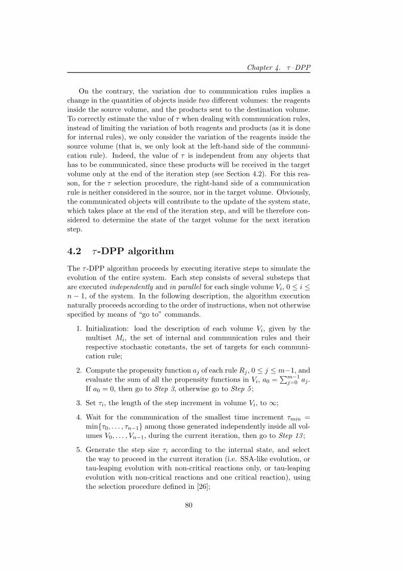
Chapter 4. τ–DPP
On the contrary, the variation due to communication rules implies achange in the quantities of objects inside two different volumes: the reagentsinside the source volume, and the products sent to the destination volume.To correctly estimate the value of τ when dealing with communication rules,instead of limiting the variation of both reagents and products (as it is donefor internal rules), we only consider the variation of the reagents inside thesource volume (that is, we only look at the left-hand side of the communi-cation rule). Indeed, the value of τ is independent from any objects thathas to be communicated, since these products will be received in the targetvolume only at the end of the iteration step (see Section 4.2). For this rea-son, for the τ selection procedure, the right-hand side of a communicationrule is neither considered in the source, nor in the target volume. Obviously,the communicated objects will contribute to the update of the system state,which takes place at the end of the iteration step, and will be therefore con-sidered to determine the state of the target volume for the next iterationstep.
4.2 τ-DPP algorithm
The τ -DPP algorithm proceeds by executing iterative steps to simulate theevolution of the entire system. Each step consists of several substeps thatare executed independently and in parallel for each single volume Vi, 0 ≤ i ≤n − 1, of the system. In the following description, the algorithm executionnaturally proceeds according to the order of instructions, when not otherwisespecified by means of “go to” commands.
1. Initialization: load the description of each volume Vi, given by themultiset Mi, the set of internal and communication rules and theirrespective stochastic constants, the set of targets for each communi-cation rule;
2. Compute the propensity function aj of each rule Rj , 0 ≤ j ≤ m−1, andevaluate the sum of all the propensity functions in Vi, a0 =
∑m−1j=0 aj.
If a0 = 0, then go to Step 3, otherwise go to Step 5 ;
3. Set τi, the length of the step increment in volume Vi, to ∞;
4. Wait for the communication of the smallest time increment τmin =minτ0, . . . , τn−1 among those generated independently inside all vol-umes V0, . . . , Vn−1, during the current iteration, then go to Step 13 ;
5. Generate the step size τi according to the internal state, and selectthe way to proceed in the current iteration (i.e. SSA-like evolution, ortau-leaping evolution with non-critical reactions only, or tau-leapingevolution with non-critical reactions and one critical reaction), usingthe selection procedure defined in [26];
80
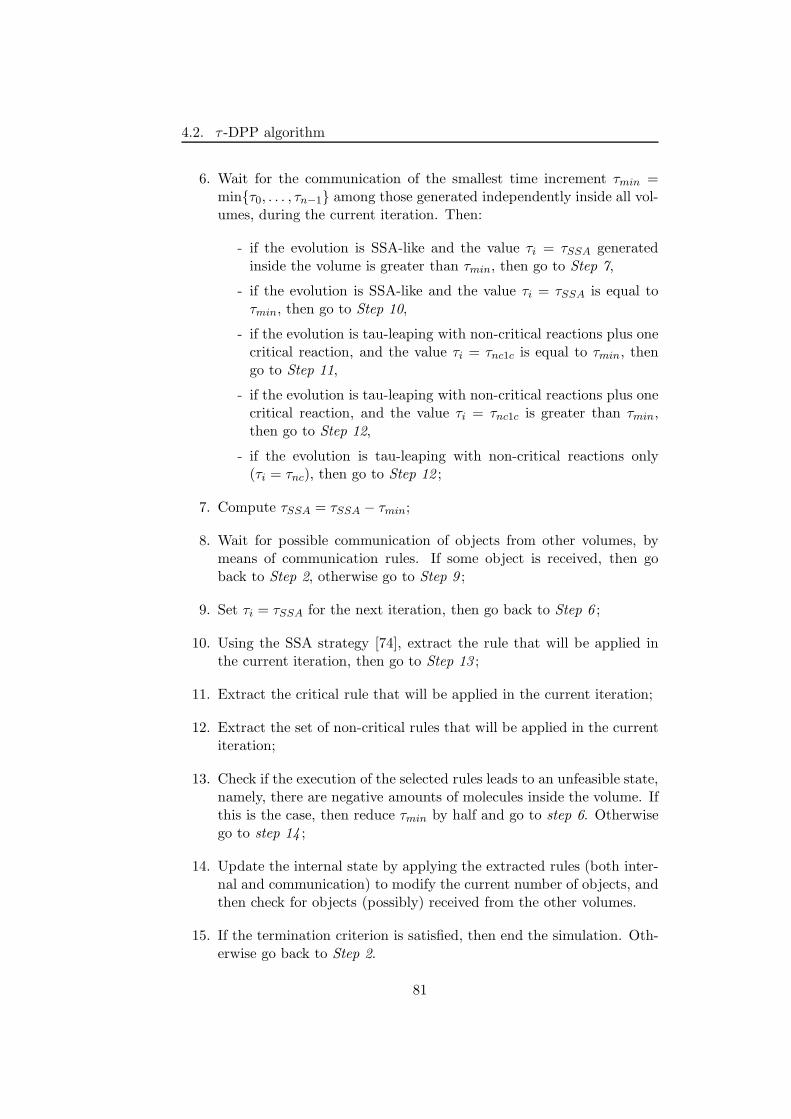
4.2. τ -DPP algorithm
6. Wait for the communication of the smallest time increment τmin =minτ0, . . . , τn−1 among those generated independently inside all vol-umes, during the current iteration. Then:
- if the evolution is SSA-like and the value τi = τSSA generatedinside the volume is greater than τmin, then go to Step 7,
- if the evolution is SSA-like and the value τi = τSSA is equal toτmin, then go to Step 10,
- if the evolution is tau-leaping with non-critical reactions plus onecritical reaction, and the value τi = τnc1c is equal to τmin, thengo to Step 11,
- if the evolution is tau-leaping with non-critical reactions plus onecritical reaction, and the value τi = τnc1c is greater than τmin,then go to Step 12,
- if the evolution is tau-leaping with non-critical reactions only(τi = τnc), then go to Step 12 ;
7. Compute τSSA = τSSA − τmin;
8. Wait for possible communication of objects from other volumes, bymeans of communication rules. If some object is received, then goback to Step 2, otherwise go to Step 9 ;
9. Set τi = τSSA for the next iteration, then go back to Step 6 ;
10. Using the SSA strategy [74], extract the rule that will be applied inthe current iteration, then go to Step 13 ;
11. Extract the critical rule that will be applied in the current iteration;
12. Extract the set of non-critical rules that will be applied in the currentiteration;
13. Check if the execution of the selected rules leads to an unfeasible state,namely, there are negative amounts of molecules inside the volume. Ifthis is the case, then reduce τmin by half and go to step 6. Otherwisego to step 14 ;
14. Update the internal state by applying the extracted rules (both inter-nal and communication) to modify the current number of objects, andthen check for objects (possibly) received from the other volumes.
15. If the termination criterion is satisfied, then end the simulation. Oth-erwise go back to Step 2.
81
Chapter 4. τ–DPP
The initialization phase of the algorithm is executed in parallel insideevery single volume of the system, where distinct rules and amounts ofobjects may appear. The computation of the propensity functions aj of therules Rj is performed exploiting the expression presented in [74]. In step 2,we check whether the sum a0 of all the propensity functions of the volumeis equal to zero. If so, then no rule can be executed inside this volume; inthis case, we set τi = ∞ and let the volume wait for the current τmin value,chosen among the time increments computed inside the other volumes. Thisstep is necessary for the synchronization between this volume and the otherones where, possibly, some rules will be applied. So doing, during the updateat the final step of the algorithm, it will also be possible to check whether thevolume is the target of some communication rules applied in other volumes(that is, whether it will receive new objects), and hence properly update itsinternal state.
On the other hand, if a0 > 0, the value of τi is computed inside thevolume considering only its internal state (this is done exploiting the firstpart of the tau-leaping procedure presented in [26]). The τi computationalso implies the selection of the kind of evolution for the current iterationinside each volume Vi, independently from the kind of evolution selected inthe other volumes.
Once every volume of the system has computed its τi value, the smallestone is selected and used to generate the evolution of the whole system (step 6of the algorithm) during the current iteration. This means that each volumewill not evolve according to the internally computed τi, but according tothe common value τmin. The rational behind this is that, we let all volumesproceed along a common time line, therefore avoiding paradoxical situationswhere one volume will execute rules that take place in the future or in thepast time of another volume.
When every volume has received the common value τmin, according tothe evolution strategy selected at step 5 of the algorithm, it extracts therules that will be applied in the final stage of the iteration. If the evolutionof the volume is governed by the SSA strategy, we have to check if τmin isequal to τi (here called τSSA). If so, it means that the chosen τmin valuewas actually generated inside this volume, and that the current iteration is“long enough” to allow the application of one rule inside this volume. Onthe other hand, if τmin < τSSA, then it is not possible to apply any ruleinside this volume. For this reason we only have to update the value of τi
(step 7 of the algorithm).Afterwards, the volume verifies for possible incoming objects: if some-
thing is received from other volumes, then the internal state of the volumeis changed, and in the next iteration the volume will compute new values ofthe propensity functions and a new τi value. On the contrary, if the volumedoes not receive anything from its adjacent volumes, then its internal stateremains unchanged. For this reason, the τi value used in the next iteration
82
4.2. τ -DPP algorithm
will be the current τSSA value (updated during the step 7 of the algorithm).Notice that the value τi = τSSA − τmin is used again in the next iterationbecause, in the case τi is the smallest time increment of the whole system,then the volume will be able to complete the execution of one rule.
The situation is easier for the other kinds of evolution. If the volumeis executing a tau-leaping step with the application of a set of non-criticalreactions and one critical reaction, we have to check if τi = τmin. If thisis true, besides the execution of the non-critical reactions extracted fromthe poissonian distributions (we refer to [26] for details), it is possible toexecute one critical reaction. Indeed, the value τi computed inside the vol-ume corresponds to the time needed to execute such critical reaction (thisis the reason why its execution is allowed). On the contrary, if τi > τmin,the volume will execute non-critical reactions only. Finally, if the volume isevolving according to the tau-leaping procedure with the execution of non-critical reactions only, we use τmin for the sampling of the number of rulesthat will be executed (according to the strategy described in [26]).
During step 13, the algorithm checks if the execution of the selectedreactions (both internal and communication) leads to an unfeasible systemstate, where negative amounts of objects appear. In this case, the strategyto avoid this problem consists in reducing the value of τmin by half and goback to step 6 of the algorithm. So doing, a new set of reactions (possiblysmaller than the previous one) will be selected. The condition about negativepopulation is checked until an appropriate set of reactions is selected, halvingeach time the length of the time step.
Finally, the state of the system is updated. Every volume executes theselected reactions, both internal and communication, hence the number ofobjects is properly updated also by means of the objects (possibly) receivedfrom the other volumes. Note that the internal states of all volumes areupdated in parallel and, thanks to the choice of the common time incrementτmin, also in a synchronized fashion.
The algorithm takes a computational time equal to that of the originaltau-leaping procedure for the simulation of a single volume, since the τcalculation strategy is the same. Hence, the time required to execute eachiteration is proportional to 2M (where M is the number of reactions of thesystem). For a generic system composed by N volumes, the computationaltime becomes 2MN , because it increases with the number of volumes itself.The complexity of τ -DPP is different from other algorithms, like the NSM,where a single volume evolves during each iteration. Indeed, in τ -DPP theinternal state of each volume has to be updated and, in order to computethe length of the time step, the contribution of the entire system is required.
On the other hand, the τ -DPP strategy can be easily coded for parallelarchitectures, where a one-to-one correspondence between volumes and pro-cesses or threads, can be obtained. In this case, the computational time ofthe algorithm scales with the number of “parallel processes” executed, with
83
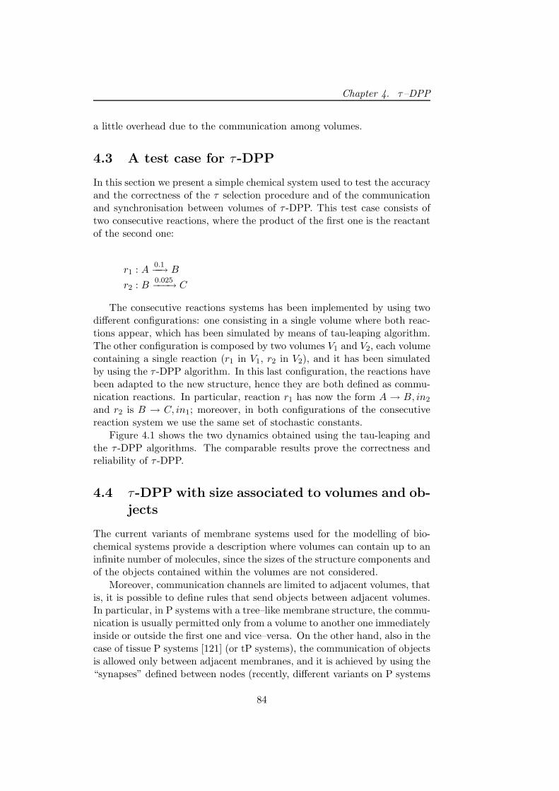
Chapter 4. τ–DPP
a little overhead due to the communication among volumes.
4.3 A test case for τ-DPP
In this section we present a simple chemical system used to test the accuracyand the correctness of the τ selection procedure and of the communicationand synchronisation between volumes of τ -DPP. This test case consists oftwo consecutive reactions, where the product of the first one is the reactantof the second one:
r1 : A0.1−−→ B
r2 : B0.025−−−→ C
The consecutive reactions systems has been implemented by using twodifferent configurations: one consisting in a single volume where both reac-tions appear, which has been simulated by means of tau-leaping algorithm.The other configuration is composed by two volumes V1 and V2, each volumecontaining a single reaction (r1 in V1, r2 in V2), and it has been simulatedby using the τ -DPP algorithm. In this last configuration, the reactions havebeen adapted to the new structure, hence they are both defined as commu-nication reactions. In particular, reaction r1 has now the form A → B, in2
and r2 is B → C, in1; moreover, in both configurations of the consecutivereaction system we use the same set of stochastic constants.
Figure 4.1 shows the two dynamics obtained using the tau-leaping andthe τ -DPP algorithms. The comparable results prove the correctness andreliability of τ -DPP.
4.4 τ-DPP with size associated to volumes and ob-
jects
The current variants of membrane systems used for the modelling of bio-chemical systems provide a description where volumes can contain up to aninfinite number of molecules, since the sizes of the structure components andof the objects contained within the volumes are not considered.
Moreover, communication channels are limited to adjacent volumes, thatis, it is possible to define rules that send objects between adjacent volumes.In particular, in P systems with a tree–like membrane structure, the commu-nication is usually permitted only from a volume to another one immediatelyinside or outside the first one and vice–versa. On the other hand, also in thecase of tissue P systems [121] (or tP systems), the communication of objectsis allowed only between adjacent membranes, and it is achieved by using the“synapses” defined between nodes (recently, different variants on P systems
84
4.4. τ -DPP with size associated to volumes and objects
0
200
400
600
800
1000
0 10 20 30 40 50 60 70 80
Mol
ecul
es
Time [s]
A
B
C
tau-DPPtau-leaping
Figure 4.1: Comparison between the dynamics of the consecutive reactionsystem obtained by means of tau-leaping (dashed lines) and τ -DPP (solidlines).
have been introduced to better model economic or socio-economic processes,databases, operating systems, etc., in which different communication strate-gies are used, like Hyperdag P systems [148], or variants like that presentedin [155]).
For what concerns the membrane structure, either variant of P systemsuse only a tree–like or a tissue–like structure, while hybrid structures arenot considered. For instance, the description of tissues where nodes canhave a complex internal structure, or tree–like systems where membranescan enclose a tissue, have never been defined.
We briefly report here the basic notions of tP systems [121]. tP sys-tems have been defined to describe a tissue–like architecture, where cells areplaced in the nodes of a (directed) graph, and objects are communicatedalong the edges of the graph. These communication channels are calledsynapses. Moreover, the communication of objects can be achieved both ina replicative and non–replicative manner, that is, objects can be sent to alladjacent cells or to one adjacent cell only, respectively.
In general, the structure of a tP system is composed by elementary mem-branes, namely, each node of the system is represented by a membrane thatdoes not contain other membranes. Furthermore, the communication ofobjects is allowed, as in standard P systems, only to/from adjacent mem-branes. We refer the interested reader to [65, 157, 4, 116, 120] for further
85
Chapter 4. τ–DPP
information and examples about tP systems.
Hereafter, we present a different variant of τ -DPP, called Sτ -DPP [29],where we associate “measures” which represent the size of volumes andobjects, we use tP systems [121] to describe the topological organisation ofthe membranes and to denote the possible communication channels of thesystem, and we exploit the simulation strategy described in Section 4.1 todescribe the behaviour of the system. In the following, we will refer withoutdistinction to membranes or volumes.
To be more precise, in Sτ -DPP we associate a measure to membranesand objects, representing the “size” of the volumes where the computa-tion occurs and the volume of each object, respectively. Both the sizes ofmembranes and objects are useful to describe any real system where it is im-portant to avoid the infinite accumulation of objects inside a compartment,which is very important in chemical system and cannot be achieved by sim-ply bounding the “capacity” of the membranes or by limiting the maximumnumber of each kind object allowed inside a particular volume, since eachobject can have a different size. Moreover, in the framework of Sτ -DPP,the system’s structure is independent from the communication channels be-tween membranes, hence, two different graphs are used in the description:the first one denotes the membrane structure, while the second graph speci-fies the connections between membranes which allow the communication ofobjects. Furthermore, the membrane structure can be hybrid (since it com-bines tree-like P systems with tissue P systems), and the communicationcan be performed between non adjacent membranes, to denote privilegedpathways between membranes. This characteristic of Sτ -DPP takes inspira-tion from a specific component of living cells, called microtubule [167], withthe aim of reproducing its role as intracellular “highway” for the transportof other cellular components, such as vesicles and proteins.
Sτ-DPP
In this section we will give a detailed description of Sτ -DPP, providing abasic definition and the algorithm used to simulate a system’s dynamics.As already said, Sτ -DPP is obtained combining the structure definition oftP systems with the simulation strategy used in τ -DPP. Here, nodes arearranged in a tissue–like fashion, but each of them can have a complex in-ternal hierarchy, organised in a tree–like structure. Moreover, in this newvariant we consider sizes for both membranes and objects, and the rulesdefined inside each membrane will be enabled only in the case there is suf-ficient free space in the membrane where the rule is applied, for instance,to “create” new objects or to receive objects from other volumes. The sizeconsidered here can be used in the modelling and simulation of biochemicalsystems where diffusive processes play an important role, and it is necessaryto avoid the unlimited accumulation of objects in a region of finite size.
86
4.4. τ -DPP with size associated to volumes and objects
In order to correctly describe the hierarchy of complex nodes of thesystem we first need a graph representing the topology of the membranes.In particular, this graph can have undirected edges to indicate that twomembranes are placed at the same hierarchical level (as in the standarddefinition of tP systems [121]). On the other hand, directed edges of thegraph are used to denote that the “source” membrane contains the “target”membrane.
A second directed graph is needed to represent the communication chan-nels among membranes. Clearly, the arrows of the edges indicate the direc-tion of the (permitted) flow of objects between different compartments. Notethat, this communication graph can contain edges that are not indicated inthe graph which describes the membrane structure. The meaning of theseparticular edges is to represent communication channels that connect nonadjacent membranes. Using these arcs, it is then possible to create privilegedpathways of communication between membranes.
The features of Sτ -DPP can be exploited to represent (among other reallife systems) reaction–diffusion systems [47], namely, mathematical modelswhich capture the dynamics of a set of substances involved in a number ofchemical reactions, considering both the temporal and spatial dimension.In this case, the membrane structure can be used to represent a reactionvolume as the composition of a number of finite size subvolumes, and thecommunication graph will describe the diffusion directions through the sys-tem.
Definition
A Sτ -DPP with sizes associated with membranes and objects is defined as
Υ = (V,TG, CG,S,M,R, C,DX ,DV ),
where:
• V = V0, . . . , Vn−1 is the set of the volumes Vi of the system;
• TG = (V, AT ) is a graph representing the topological arrangement ofthe volumes in V and AT = Au
T ∪AdT is the set of the arcs (Vl, Vk) which
describes the arrangement of volumes. In particular, AuT is the subset
of undirected arcs representing the connections between membranesplaced at the same level in the membrane structure. On the contrary,Ad
T is the set of directed arcs (Vl, Vk) (where Vk ∈ Vl) which specifiesthe inclusion relations between volumes. We also define the set of thevolumes enclosed in Vi as aT (Vi) = Vl | Vl ∈ V, (Vi, Vl) ∈ Ad
T ;
• CG = (V, AC) is a directed graph representing the connections (commu-nication channels) among the volumes in V. AC is the set of directed
87
Chapter 4. τ–DPP
arcs (Vl, Vk) (from Vl to Vk) which denote the presence of communi-cation channels between volumes and specify in which directions theflow of objects is allowed;
• S = X1, . . . ,XM is the set of molecular species, that is, the alphabetof the system;
• M = M0, . . . ,Mn−1, is the set of the multisets occurring insidethe membranes V0, . . . , Vn−1, representing the internal state of thevolumes. Each multiset Mi (0 ≤ i ≤ n − 1) is defined over S;
• R = R0, . . . , Rn−1 is the set of the sets of rules defined in volumesV0, . . . , Vn−1, respectively. A rule can be of internal or of communica-tion type (as described below);
• C = C0, . . . , Cn−1 is the set of the sets of stochastic constants asso-ciated to the rules defined in volumes V0, . . . , Vn−1;
• DX = DX1, . . . ,DXM
, with DXj∈ R
+, is the set of the sizes of themolecular species X1, . . . ,XM , respectively;
• DV = DV0, . . . ,DVn−1
, with DVi∈ R
+, is the set of the sizes of thevolume V0, . . . , VN , respectively.
The multiset Mi, describing the state of volume Vi (i = 0, . . . , n − 1), isdefined as Mi = (m0, . . . ,mM ) where mj denotes the number of moleculesof the species Xj occurring inside Vi (j = 1, . . . ,M).
Given the internal state Mi of a membrane Vi together with the speciessizes in DX , it is possible to define the occupied volume in Vi as:
O(Vi) =M∑
j=1
(mj · DXj) +
∑
Vl∈aT (Vi)
DVl, (4.1)
O(Vi) denotes the volume occupied by the objects currently present insidevolume Vi.
Hence, it is possible to define the value of the free space in Vi as:
F (Vi) = DVi− O(Vi) (4.2)
Note that, at each rule execution (internal or communication), the freespace value has to be updated. The update operation adds to the freespace value the “volume” of the objects consumed or sent by the rule andsubtracts the “volume” of the objects produced by the rule or received fromother membranes. Internal rules have the general form α1X1 +α2X2 + · · ·+αMXM → β1X1 + β2X2 + · · · + βMXM , after the execution of this kindof rules, the free space in Vi is updated as F (Vi) = F (Vi) −
∑Mj=1(βj −
αj) · DXj. On the contrary, a communication rule, have the generic form
88
4.4. τ -DPP with size associated to volumes and objects
α1X1 + α2X2 + · · · + αMXM → (β1,1X1 + · · · + βM,1XM , tgt1) + (β1,2X1 +· · ·+ βM,2XM , tgt2) + · · ·+ (β1,NX1 + · · ·+ βM,NXM , tgtN ). In this case weneed to update the free space of Vi (i.e., the membrane where the reaction isapplied) as F (Vi) = F (Vi)+
∑Mj=1 αj ·DXj
and the free space of each target
volume Vtgtk indicated by the rule: F (Vtgtk ) = F (Vtgtk )−∑M
j=1 βj,kDXj≥ 0.
In order to obtain a correct description of the system’s dynamics, we needto check if a rule rµ (internal or communication) is applicable. Therefore, weneed to compute the effect of a rule on the free space of the volume affectedby the rule. It is clear that a rule can be executed only if the free space ofthe volume, after the rule application, is greater or equal to zero. The ruleapplicability is computed differently for internal and communication rules.Given an internal rule occurring inside volume Vi, we need to check if, afterthe rule execution, F (Vi) ≥ 0. For what concerns a communication rule rµ,we need to check all the free space of the target volumes indicated by therule: ∀ tgtl of rµ, F (Vtgtl) ≥ 0, where the values βj are the stoichiometriccoefficients of the molecular species associated with Vtgtl .
Note that, using a strategy based on the tau-leaping algorithm to de-scribe the behaviour of the system, at each iteration step, a certain numberof rules is applied in parallel. Hence, the applicability of the entire set of se-lected rules need to be verified. This operation is realised by computing thefree values of each volume Vi considering the contribution of all the selectedrules; if the values of F (Vi) is greater or equal to zero (for each volume), thenthe execution is allowed; otherwise a new set of rules need to be selected.
The algorithm
The Sτ -DPP algorithm is based on the original τ -DPP procedure presentedin Section 4.2. The differences between the two algorithms regard the specificoperations defined in order to handle the size of membrane and objects, tocompute the free space of each membrane and to check the applicability ofthe selected rules.
In particular, at the beginning of the computation the Sτ -DPP algo-rithms needs to initialise the volume by loading all the information relatedto the size of membranes and objects in order to compute the initial valueof the free space. The other step of the iterative cycle are the same as in τ -DPP, since the “sizes” are not involved in the computation of the propensityfunctions and in the rules selection.
On the other hand, in the final step of Sτ -DPP, we need to verify ifthe execution of the selected set of rules leads to an unfeasible state of thesystem, with negative values of the free spaces of the membranes. This phaseof the algorithm is realised by computing, inside each volume, the new valueof the free space considering the contribution of the selected rules, bothinternal and communication. If there is at least one volume whose freespace value is negative, then the execution of the rules is not allowed. In
89
Chapter 4. τ–DPP
this case, the value of the length of the step τ is reduced by half, and anew (possibly smaller) set of rules is selected. This operations are repeateduntil the condition on the free space is satisfied (i.e., no negative free spacevalues are present). Note that this strategy is the same used when negativeamounts of objects appear in the system.
Finally, the system is updated according to the selected rules by modi-fying the objects amounts and the values of the free space of each volume.
The other features introduced in Sτ -DPP regarding the possibility tosend objects to non-adjacent membranes and the definition of hybrid mem-brane structure do not affect the simulation procedure, since they are im-plicitly considered in the algorithm.
4.5 A test case for Sτ-DPP
In this section we present a system with preferential communication path-ways. In particular, we define a model in which it is present a so calledmicrotubule [167]. The microtubule is a sort of intracellular “highway” forthe transport of other cellular components, such as vesicles and proteins.In order to define a preferential pathway, we exploit the communication be-tween non adjacent membranes to move objects in particular directions. Weconsider the membrane system Υ represented in Figure 4.2, where:
• V = V0, . . . , V7;
• TG = (V, AT ), where AuT = (V2, V3), (V4, V5), (V6, V7), and Ad
T =(V0, V1), (V1, V2), (V1, V3), (V3, V4), (V3, V5), (V5, V6), (V5, V7);
• CG = (V, AC), AC = (V0, V1), (V1, V0), (V1, V2), (V1, V3), (V3, V1),(V3, V2), (V3, V4), (V3, V5), (V5, V3), (V5, V4), (V5, V6), (V5, V7), (V7, V5),(V6, V7);
• S = X1,X2;
• M = M0, . . . ,M7, M0 = X105
1 ,X105
2 , M3 = M4 = . . . = M7 = ∅;
• R = R0, . . . , R7, R0 = r0,0, r0,1, R1 = r1,0, . . . , r1,4, R2 = r2,0,R3 = r3,0, . . . , r3,2, . . . , r3,4, R4 = r4,0, R5 = r5,0, . . . , r5,4, R6 =r6,0, R7 = r7,0, . . . , r7,4;
• C = C0, . . . , C7, where the value of all the stochastic constants is setto 1;
• DX = 1, 1;
• DV = 106, 11 · 104, 104, 106, 8 · 104, 5 · 104, 104, 2 · 104.
90
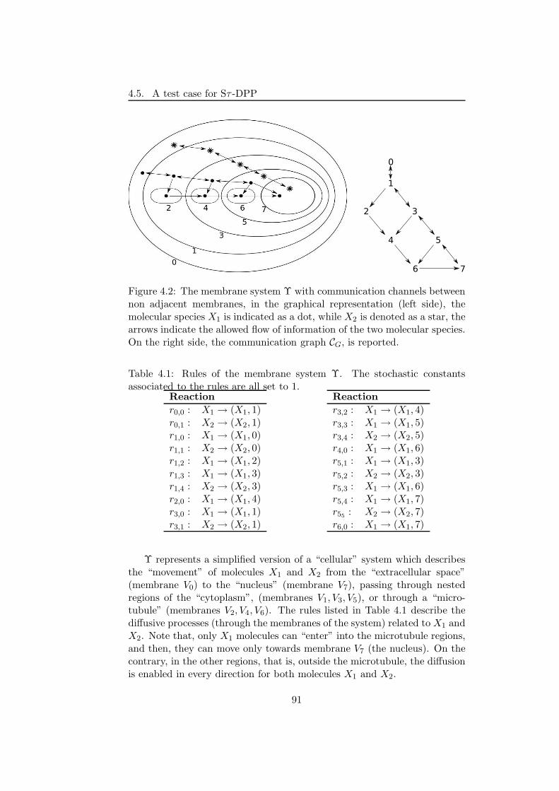
4.5. A test case for Sτ -DPP
Figure 4.2: The membrane system Υ with communication channels betweennon adjacent membranes, in the graphical representation (left side), themolecular species X1 is indicated as a dot, while X2 is denoted as a star, thearrows indicate the allowed flow of information of the two molecular species.On the right side, the communication graph CG, is reported.
Table 4.1: Rules of the membrane system Υ. The stochastic constantsassociated to the rules are all set to 1.
Reaction
r0,0 : X1 → (X1, 1)r0,1 : X2 → (X2, 1)r1,0 : X1 → (X1, 0)r1,1 : X2 → (X2, 0)r1,2 : X1 → (X1, 2)r1,3 : X1 → (X1, 3)r1,4 : X2 → (X2, 3)r2,0 : X1 → (X1, 4)r3,0 : X1 → (X1, 1)r3,1 : X2 → (X2, 1)
Reaction
r3,2 : X1 → (X1, 4)r3,3 : X1 → (X1, 5)r3,4 : X2 → (X2, 5)r4,0 : X1 → (X1, 6)r5,1 : X1 → (X1, 3)r5,2 : X2 → (X2, 3)r5,3 : X1 → (X1, 6)r5,4 : X1 → (X1, 7)r55
: X2 → (X2, 7)r6,0 : X1 → (X1, 7)
Υ represents a simplified version of a “cellular” system which describesthe “movement” of molecules X1 and X2 from the “extracellular space”(membrane V0) to the “nucleus” (membrane V7), passing through nestedregions of the “cytoplasm”, (membranes V1, V3, V5), or through a “micro-tubule” (membranes V2, V4, V6). The rules listed in Table 4.1 describe thediffusive processes (through the membranes of the system) related to X1 andX2. Note that, only X1 molecules can “enter” into the microtubule regions,and then, they can move only towards membrane V7 (the nucleus). On thecontrary, in the other regions, that is, outside the microtubule, the diffusionis enabled in every direction for both molecules X1 and X2.
91
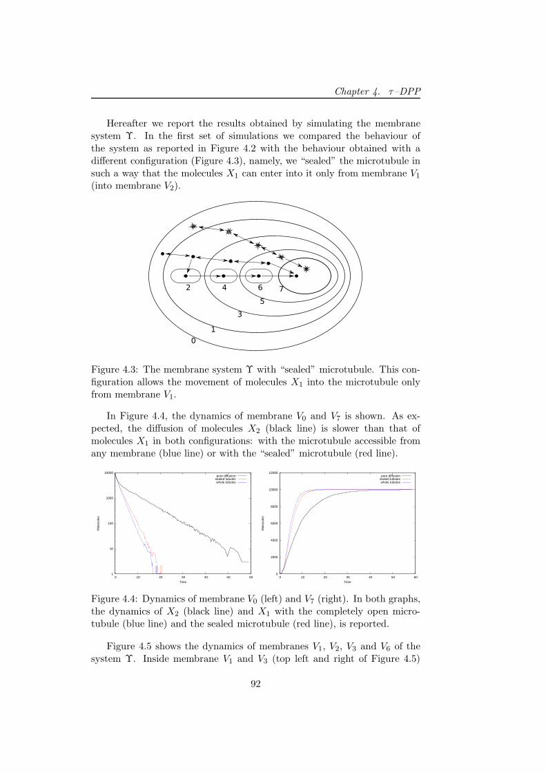
Chapter 4. τ–DPP
Hereafter we report the results obtained by simulating the membranesystem Υ. In the first set of simulations we compared the behaviour ofthe system as reported in Figure 4.2 with the behaviour obtained with adifferent configuration (Figure 4.3), namely, we “sealed” the microtubule insuch a way that the molecules X1 can enter into it only from membrane V1
(into membrane V2).
Figure 4.3: The membrane system Υ with “sealed” microtubule. This con-figuration allows the movement of molecules X1 into the microtubule onlyfrom membrane V1.
In Figure 4.4, the dynamics of membrane V0 and V7 is shown. As ex-pected, the diffusion of molecules X2 (black line) is slower than that ofmolecules X1 in both configurations: with the microtubule accessible fromany membrane (blue line) or with the “sealed” microtubule (red line).
1
10
100
1000
10000
0 10 20 30 40 50 60
Mol
ecul
es
Time
pure diffusionsealed tubuleswhole tubules
0
2000
4000
6000
8000
10000
12000
0 10 20 30 40 50 60
Mol
ecul
es
Time
pure diffusionsealed tubuleswhole tubules
Figure 4.4: Dynamics of membrane V0 (left) and V7 (right). In both graphs,the dynamics of X2 (black line) and X1 with the completely open micro-tubule (blue line) and the sealed microtubule (red line), is reported.
Figure 4.5 shows the dynamics of membranes V1, V2, V3 and V6 of thesystem Υ. Inside membrane V1 and V3 (top left and right of Figure 4.5)
92
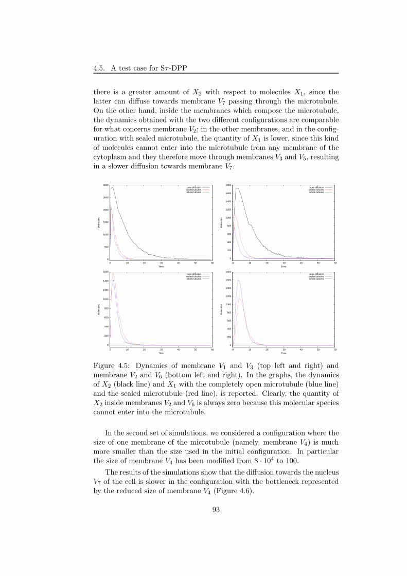
4.5. A test case for Sτ -DPP
there is a greater amount of X2 with respect to molecules X1, since thelatter can diffuse towards membrane V7 passing through the microtubule.On the other hand, inside the membranes which compose the microtubule,the dynamics obtained with the two different configurations are comparablefor what concerns membrane V2; in the other membranes, and in the config-uration with sealed microtubule, the quantity of X1 is lower, since this kindof molecules cannot enter into the microtubule from any membrane of thecytoplasm and they therefore move through membranes V3 and V5, resultingin a slower diffusion towards membrane V7.
0
500
1000
1500
2000
2500
3000
0 10 20 30 40 50 60
Mol
ecul
es
Time
pure diffusionsealed tubuleswhole tubules
0
200
400
600
800
1000
1200
1400
1600
1800
0 10 20 30 40 50 60
Mol
ecul
es
Time
pure diffusionsealed tubuleswhole tubules
0
200
400
600
800
1000
1200
1400
1600
0 10 20 30 40 50 60
Mol
ecul
es
Time
pure diffusionsealed tubuleswhole tubules
0
200
400
600
800
1000
1200
1400
1600
1800
0 10 20 30 40 50 60
Mol
ecul
es
Time
pure diffusionsealed tubuleswhole tubules
Figure 4.5: Dynamics of membrane V1 and V3 (top left and right) andmembrane V2 and V6 (bottom left and right). In the graphs, the dynamicsof X2 (black line) and X1 with the completely open microtubule (blue line)and the sealed microtubule (red line), is reported. Clearly, the quantity ofX2 inside membranes V2 and V6 is always zero because this molecular speciescannot enter into the microtubule.
In the second set of simulations, we considered a configuration where thesize of one membrane of the microtubule (namely, membrane V4) is muchmore smaller than the size used in the initial configuration. In particularthe size of membrane V4 has been modified from 8 · 104 to 100.
The results of the simulations show that the diffusion towards the nucleusV7 of the cell is slower in the configuration with the bottleneck representedby the reduced size of membrane V4 (Figure 4.6).
93
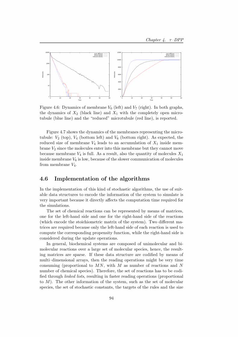
Chapter 4. τ–DPP
1
10
100
1000
10000
0 10 20 30 40 50 60
Mol
ecul
es
Time
pure diffusionwhole tubules
reduced tubules
0
2000
4000
6000
8000
10000
12000
0 10 20 30 40 50 60
Mol
ecul
es
Time
pure diffusionwhole tubules
reduced tubules
Figure 4.6: Dynamics of membrane V0 (left) and V7 (right). In both graphs,the dynamics of X2 (black line) and X1 with the completely open micro-tubule (blue line) and the “reduced” microtubule (red line), is reported.
Figure 4.7 shows the dynamics of the membranes representing the micro-tubule: V2 (top), V4 (bottom left) and V6 (bottom right). As expected, thereduced size of membrane V4 leads to an accumulation of X1 inside mem-brane V2 since the molecules enter into this membrane but they cannot movebecause membrane V4 is full. As a result, also the quantity of molecules X1
inside membrane V6 is low, because of the slower communication of moleculesfrom membrane V4.
4.6 Implementation of the algorithms
In the implementation of this kind of stochastic algorithms, the use of suit-able data structures to encode the information of the system to simulate isvery important because it directly affects the computation time required forthe simulations.
The set of chemical reactions can be represented by means of matrices,one for the left-hand side and one for the right-hand side of the reactions(which encode the stoichiometric matrix of the system). Two different ma-trices are required because only the left-hand side of each reaction is used tocompute the corresponding propensity function, while the right-hand side isconsidered during the update operations.
In general, biochemical systems are composed of unimolecular and bi-molecular reactions over a large set of molecular species, hence, the result-ing matrices are sparse. If these data structure are codified by means ofmulti–dimensional arrays, then the reading operations might be very timeconsuming (proportional to MN , with M as number of reactions and Nnumber of chemical species). Therefore, the set of reactions has to be codi-fied through linked lists, resulting in faster reading operations (proportionalto M). The other information of the system, such as the set of molecularspecies, the set of stochastic constants, the targets of the rules and the size
94
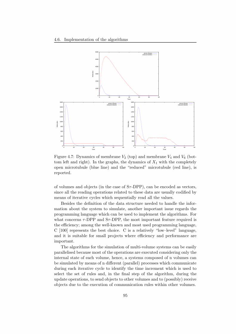
4.6. Implementation of the algorithms
0
1000
2000
3000
4000
5000
6000
0 10 20 30 40 50 60
Mol
ecul
es
Time
whole tubulesreduced tubules
0
200
400
600
800
1000
1200
1400
1600
1800
0 10 20 30 40 50 60
Mol
ecul
es
Time
whole tubulesreduced tubules
0
200
400
600
800
1000
1200
1400
1600
1800
0 10 20 30 40 50 60
Mol
ecul
es
Time
whole tubulesreduced tubules
Figure 4.7: Dynamics of membrane V2 (top) and membrane V4 and V6 (bot-tom left and right). In the graphs, the dynamics of X1 with the completelyopen microtubule (blue line) and the “reduced” microtubule (red line), isreported.
of volumes and objects (in the case of Sτ -DPP), can be encoded as vectors,since all the reading operations related to these data are usually codified bymeans of iterative cycles which sequentially read all the values.
Besides the definition of the data structure needed to handle the infor-mation about the system to simulate, another important issue regards theprogramming language which can be used to implement the algorithms. Forwhat concerns τ -DPP and Sτ -DPP, the most important feature required isthe efficiency; among the well-known and most used programming language,C [100] represents the best choice. C is a relatively “low–level” language,and it is suitable for small projects where efficiency and performance areimportant.
The algorithms for the simulation of multi-volume systems can be easilyparallelised because most of the operations are executed considering only theinternal state of each volume, hence, a systems composed of n volumes canbe simulated by means of n different (parallel) processes which communicateduring each iterative cycle to identify the time increment which is used toselect the set of rules and, in the final step of the algorithm, during theupdate operations, to send objects to other volumes and to (possibly) receiveobjects due to the execution of communication rules within other volumes.
95
Chapter 4. τ–DPP
The coding of the τ -DPP and Sτ -DPP has been realised exploiting themessage passing interface (MPI) [142]. MPI represents a standard for com-munication among processes that model a parallel program running on adistributed memory system. Among others, actual distributed memory su-percomputers, such as clusters, are suitable for the execution of these pro-grams.
4.7 Discussion and future developments
In this chapter we have shown how the stochastic method based on the tau-leaping procedure can be implemented within the framework of P systems,for the simulation of complex biological systems. In particular, we haveconsidered the class of dynamical probabilistic P systems, to exploit thepossibility of modelling systems composed by several volumes.
The new τ selection procedure here introduced works by selecting thesmallest τ taken from the set of τs generated inside the membranes duringthe current iteration; then, an evolution step is performed executing severalrules, which are selected following the procedure presented in Section 4.1.
The advantage of introducing the tau-leaping method inside DPPs isthat we can choose the same leap of length τ for all the volumes in orderto communicate objects in the right way (assuming that they are sent tothe other volumes just at the end of each step, because the execution orderdoes not matter); this strategy results in a synchronisation of the volumesand allows to obtain a good approximation of the behaviour of the entiresystem.
An important aspect is that we can trace the simulated time of thewhole system, since every membrane evolves according to the chosen com-mon τ value. Moreover, the time needed to run the simulation with the newprocedure is the same as the original tau-leaping algorithm [26] for a singlevolume. Increasing the number of volumes, the computational time requiredincreases linearly; however, it is very easy to run a simulation on a parallelarchitecture, simulating one compartment as one process.
In the second part of this chapter we presented a new version of τ -DPP,called Sτ -DPP. The novel properties of Sτ -DPP consist in the representationof the membranes structure and the communication within the system’s vol-umes using two distinct directed graphs, the possibility to define tissue–likestructure where nodes have a complex internal architecture, the associationof a size to objects and membranes and the consequent handling of the freespace during the system evolution.
This new features are suitable for the modelling of a number of realsystems in which, first of all, the unlimited accumulation of objects withinmembranes is not possible or, in other words, where the free space withinregions is a critical resource for the system dynamics. Second, the use of two
96
4.7. Discussion and future developments
distinct graphs to describe the membranes structure and the communicationwithin the system provides a formalism with a strong expressive power:indeed it is possible to have communication channels between membranesthat are non adjacent and, conversely, it is possible that adjacent membranesdo not communicate. The first possibility allows the creation of preferentialpaths of communication, and can be used, for instance, to reproduce therole of microtubules in the protein transport within cells.
The approaches proposed in this chapter open several interesting re-search lines, ranging from the modelling of real cellular processes or complexbiological systems in general, to the algorithmic improvements of the pro-cedure, and the development of other relevant (modelling and simulating)features in the area of Membrane Computing.
As a possible future development, we can better characterise and studythe role of space occupation and diffusion of molecules among the volumesof the modelled systems. Furthermore, the simulation algorithm can be op-timised in order to obtain a more efficient procedure and, otherwise, alterna-tive strategies to select the reactions and to handle the reaction applicabil-ity can be tested. For instance, we believe that more accurate simulationsmight be achieved by considering the right–hand sides of communicationrules, during the computation of the time step τ , within the target volumes.
In addition, the problem of the size of volumes changing in time shouldalso be addressed, especially when dealing with cellular processes spanningthe cell cycle period. In fact, in this case the dimensions of volume canincrease, and also its internal conditions can be modified, therefore the req-uisite condition of fixed volume for the applicability of standard stochasticalgorithms fails.
Finally, another possible extension is represented by the considerationof the membrane potential that influences the dynamics of some biologicalsystems [45, 62]. We presented a first study about this topic in [141], where amodel for the simulation of the action potential in nervous systems, has beendescribed. Moreover, the τ -DPP algorithm has been modified in order toconsider, during the computation of the propensity functions, the influenceof the membrane potential on the probability to fire a reaction.
97

Chapter 4. τ–DPP
98
Chapter 5
Modelling chemical andbiological systems
Cellular processes are characterized by peculiar features which make themboth fascinating and challenging to be studied, either with experimentalor computational approaches. To the aim of understanding the complextopology of a biological system and its dynamics, mathematical modelinghas extensively proven to represent an indispensable tool [128, 198]. Math-ematical modeling can be broadly classified into deterministic continuousapproaches, based on the laws of mass action, and into stochastic discreteapproaches, which take into consideration the discrete character of the bio-chemical components and the intrinsic randomness of biological phenomena.Indeed, biological systems can involve a huge number of processes, but theamount of many molecular species can be very low. Under these conditions,deterministic approaches are pushed to their limits and cannot always berelied on, while stochastic methods are able to account for the randomnessthat emerges and dominates the global behaviour of the system, thus in-ducing substantial cell–cell phenotypic variations and cellular heterogeneity[59, 111].
In this chapter, different applications of τ -DPP related to the modelling,simulation and analysis of biological and chemical systems will be presented.
In Section 5.1, we present a discrete mathematical model for the Ras/-cAMP/PKA pathway in the yeast Saccharomyces cerevisiae, which is in-volved in the regulation of metabolism and cell cycle progression. Thepathway is tightly regulated by several control mechanisms, acting throughfeedback cycles on the proteins that initiate the cascade events of signaltransduction. This system is investigated under various conditions, in orderto test how different values of several stochastic reaction constants affect thepathway behaviour. In particular, we show that the level of two elementsof this pathway, the guanine nucleotides GTP and GDP, could be relevantmetabolic signals for the regulation of the whole system.
99
Chapter 5. Modelling chemical and biological systems
In Section 5.2, a model of a genetic oscillator coupled with a quorumsensing intercellular mechanism [58, 67] will be considered. The results ofsimulations will be presented; some further issues concerning future exten-sions of the model, as well as different strategies to work out the problemsof modelling a genetic oscillator, will be discussed.
In Section 5.3 we introduce the framework of chemical computing, inorder to show how to describe computations by means of chemical reactionsystems. We will present the encoding of simple boolean functions, of theFredkin gate and of Fredkin circuits, we also propose an encoding for registermachines instructions, and we give some insights about the construction ofa complete register machine with n registers. Finally, we will discuss someimprovements of this work, with the final aim of arriving at a possible wetimplementation of τ–DPP using the micro reactors technology.
Finally, in Section 5.4, the modelling and stochastic simulations of thechemotactic signal transduction pathway in bacteria, are presented. Thisparticular pathway allows bacteria to respond and adapt to environmen-tal changes, by tuning the tumbling and running motions that are due toclockwise and counterclockwise rotations of their flagella.
By exploiting τ–DPP, we analyse this system to consider the interplaybetween the stochastic fluctuations of a pivotal protein amount and thenumber of cellular flagella. This approach suggests that the combination ofthese factors might represent a relevant component for this pathway. Someissues for future extension of this work are finally discussed.
100
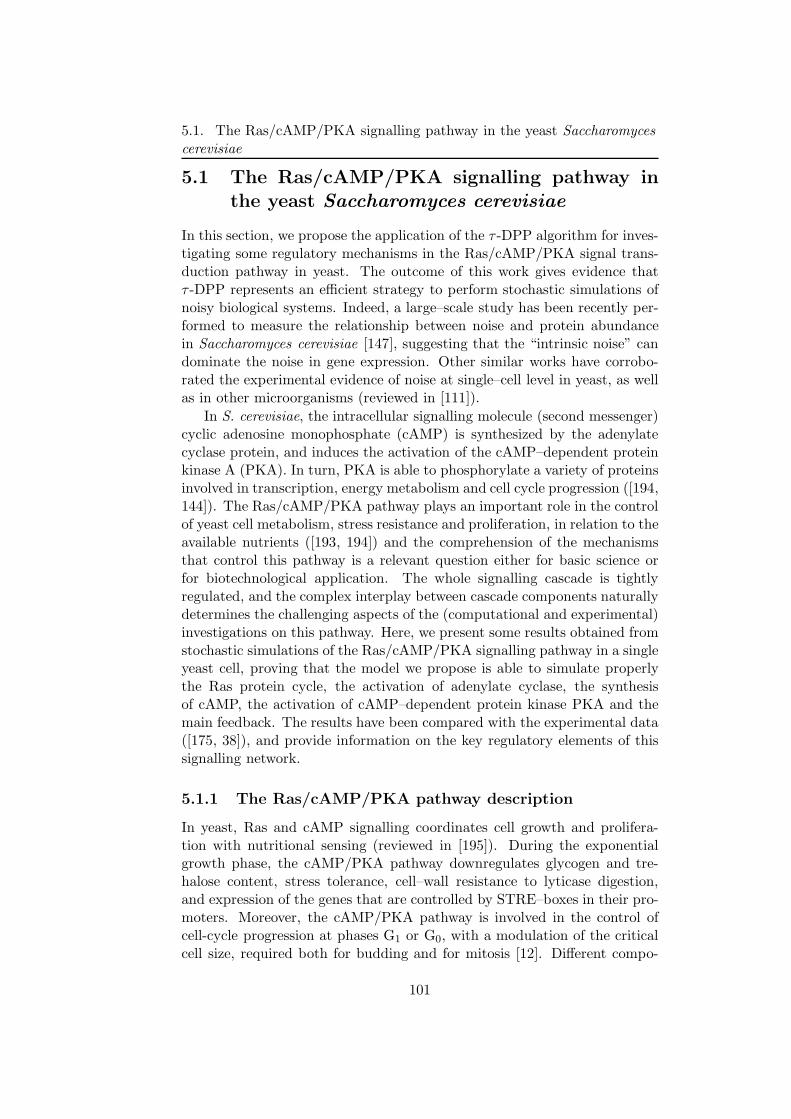
5.1. The Ras/cAMP/PKA signalling pathway in the yeast Saccharomycescerevisiae
5.1 The Ras/cAMP/PKA signalling pathway inthe yeast Saccharomyces cerevisiae
In this section, we propose the application of the τ -DPP algorithm for inves-tigating some regulatory mechanisms in the Ras/cAMP/PKA signal trans-duction pathway in yeast. The outcome of this work gives evidence thatτ -DPP represents an efficient strategy to perform stochastic simulations ofnoisy biological systems. Indeed, a large–scale study has been recently per-formed to measure the relationship between noise and protein abundancein Saccharomyces cerevisiae [147], suggesting that the “intrinsic noise” candominate the noise in gene expression. Other similar works have corrobo-rated the experimental evidence of noise at single–cell level in yeast, as wellas in other microorganisms (reviewed in [111]).
In S. cerevisiae, the intracellular signalling molecule (second messenger)cyclic adenosine monophosphate (cAMP) is synthesized by the adenylatecyclase protein, and induces the activation of the cAMP–dependent proteinkinase A (PKA). In turn, PKA is able to phosphorylate a variety of proteinsinvolved in transcription, energy metabolism and cell cycle progression ([194,144]). The Ras/cAMP/PKA pathway plays an important role in the controlof yeast cell metabolism, stress resistance and proliferation, in relation to theavailable nutrients ([193, 194]) and the comprehension of the mechanismsthat control this pathway is a relevant question either for basic science orfor biotechnological application. The whole signalling cascade is tightlyregulated, and the complex interplay between cascade components naturallydetermines the challenging aspects of the (computational and experimental)investigations on this pathway. Here, we present some results obtained fromstochastic simulations of the Ras/cAMP/PKA signalling pathway in a singleyeast cell, proving that the model we propose is able to simulate properlythe Ras protein cycle, the activation of adenylate cyclase, the synthesisof cAMP, the activation of cAMP–dependent protein kinase PKA and themain feedback. The results have been compared with the experimental data([175, 38]), and provide information on the key regulatory elements of thissignalling network.
5.1.1 The Ras/cAMP/PKA pathway description
In yeast, Ras and cAMP signalling coordinates cell growth and prolifera-tion with nutritional sensing (reviewed in [195]). During the exponentialgrowth phase, the cAMP/PKA pathway downregulates glycogen and tre-halose content, stress tolerance, cell–wall resistance to lyticase digestion,and expression of the genes that are controlled by STRE–boxes in their pro-moters. Moreover, the cAMP/PKA pathway is involved in the control ofcell-cycle progression at phases G1 or G0, with a modulation of the criticalcell size, required both for budding and for mitosis [12]. Different compo-
101
Chapter 5. Modelling chemical and biological systems
nents of the Ras/cAMP/PKA signalling pathway can be affected by stress,and contribute to the control of the cellular response. The feeding of glucose(or a related fermentable sugar) to starved S. cerevisiae cells, or the induc-tion of intracellular acidification, increase the activity of adenylate cyclaseprotein, which then triggers a rapid and transient increase in cAMP levels[193].
In yeast, this pathway is tightly regulated (Figure 5.1). The synthesisof cAMP by adenylate cyclase, CYR1, requires the activation of the smallGTPases Ras1 and Ras2, two monomeric G proteins which are inactive inthe GDP–bound state and active when GTP is bound. Ras proteins are pos-itively controlled by the guanine nucleotide exchange factor (GEFs), Cdc25and Sdc25, which stimulate the GDP-GTP exchange on Ras, and nega-tively regulated by the two GTPase activating proteins (GAPs), Ira1 andIra2, which promote the intrinsically low Ras GTPase activity. Additionally,adenylate cyclase activity is also positively modulated by the heterotrimericGTPase subunit Gpa2 and by the cognate receptor Gpr1, in response toglucose addition ([37, 175]) (see Figure 5.1).
Figure 5.1: The cAMP pathway in yeast.
The protein kinase A (PKA) is the regulatory target of cAMP, whichactivates the two catalytic subunits of PKA encoded redundantly by TPK1,TPK2 and TPK3 genes ([197, 144]) by binding to its two regulatory subunits(encoded by BCY1 gene). The active PKA operates in downstream intracel-lular signalling, through the phosphorylation of a variety of proteins involvedin transcription, energy metabolism and cell cycle progression ([194, 144])(Figure 5.1).
The inactivation of cAMP (i.e., the conversion to the form AMP) is gov-erned by the phosphodiesterases Pde1 and Pde2, two enzymes which act asantagonists in signalling in yeast and which constitute the major feedback
102
5.1. The Ras/cAMP/PKA signalling pathway in the yeast Saccharomycescerevisiae
control in the Ras/cAMP/PKA pathway ([112, 180]). This strong mecha-nism operates to rapidly downregulate the pathway, and S. cerevisiae mu-tant cells in which this feedback is inactivated can accumulate large amountsof cAMP ([150]). The cAMP phosphodiesterase Pde1, that is activated byPKA via phosphorylation ([112]), is one of the known target of this feedback,though there are indications that the feedback operates at multiple levels,also modulating the activity of Cdc25 ([81]), Ras or Ira proteins ([38]) in anot clarified manner.
The experimental studies on the Ras/cAMP/PKA pathway are compli-cated by the fact that both Ras and Cdc25 proteins are not only requiredfor glucose activation of cAMP synthesis, but they are also essential forbasal adenylate cyclase activity and for cell viability. Therefore, suppress-ing mutations, or multicopy suppressor genes restoring viability, have to bepresent in cells deleted for Ras or Cdc25. These suppressors might affectcAMP accumulation by causing enhanced feedback inhibition or by otherunknown means, causing the occurrence of some contradictory results. Re-cently, Cdc25 has been shown to be essential for Ras2 activation upon glu-cose addition ([38]) and consequent PKA activation. However, the signalsthat activate Cdc25 remain elusive, although there are some indications thatthe level of guanine nucleotides (GTP and GDP) could be a relevant inputsignal for this pathway ([177]).
5.1.2 The stochastic model
The model represents the Ras/cAMP/PKA pathway in a single yeast cell, itconsists of 30 molecular species and is described by the 34 reactions of Table5.1, where the following notation is used to describe biochemical reactions:Xp means that the molecular species X is phosphorylated, X + Y denotesan interaction between species X and Y , while X • Y denotes that speciesX and Y are chemically bound in the formation of a complex.
In order to decrease the total number of molecular species, and henceto lower the computational time, we consider only one Ras protein, Ras2(the most abundant in yeast), and only one GAP, Ira2. The regulatory andcatalytic subunits of PKA are denoted by symbols R and C, respectively.
Four main logical modules can be identified in the model:
(1) The switch cycle of Ras2 protein, involving the GEF Cdc25 and theGAP Ira2, described by reactions r1, . . . , r10.
Ras2 • GDP + Cdc25 Ras2 • GDP • Cdc25 Ras2 • Cdc25 + GDP
↓↑Ras2 • GTP + Cdc25 Ras2 • GTP • Cdc25 Ras2 • Cdc25 + GTP
The nucleotide exchange cycle has been derived by using the dataprovided in [84, 104, 177], which show the existence of a nucleotidefree Ras • Cdc25 complex that can generate either Ras • GDP or
103
Chapter 5. Modelling chemical and biological systems
Ras • GTP with similar kinetics, suggesting that the “exchange” isdependent on the concentration of available nucleotides and is not“directional” toward the generation of Ras • GTP .
(2) The synthesis of cAMP, via activation of adenylate cyclase CYR1,described by reactions r11, . . . , r13. This is modeled assuming thatadenylate cyclase (CYR1) is active only in a complex with Ras2 •GTP . The reaction r13 is optional and include a cyclase–dependentinteraction of Ras2 with Ira, as suggested by some experiments [119].
(3) The activation of PKA, via the reversible binding between its regu-latory subunits R and cAMP, and the subsequent dissociation of thetetramer PKA, described by reactions r14, . . . , r24.
(4) The activity of phosphodiesterases Pde1 and Pde2 (the latter is activein the basal level regulation of cAMP), which determines the feedbackmechanisms for cAMP degradation, described by reactions r25, . . . , r32.A Michaelis–Menten kinetics is simulated for Pde1 and Pde2. A phos-phatase activity (PPA2) is also introduced to reset the system. Inaddition, reactions r33 and r34 include an additional feedback mech-anism based on the phosphorylation/dephosphorylation of Cdc25, assuggested in [81].
The number of molecules for Ras2, Cdc25, PKA, Pde1, Pde2 and PPA2was obtained by using the data of [70] (available online at [205]).
The number for Ira2 and CYR1 was estimated by comparing the fluores-cence of yeast cells expressing fusion with eGFP (obtained by [205]) usingCdc25–eGFP as a standard (300 molecules/cell).
The number of ATP, GTP and GDP was calculated by data of [177],considering an average cell volume of 45fL [27, 96]. Taking into accountthat part of the volume is given by cell wall and by internal structures, weestimated an internal free water volume V of about 30fL (3 × 10⁻¹⁴L).
Therefore, for ATP (considering a concentration of 1mM) we obtainedabout 2 × 10⁷ molecules/cell, while for GTP and GDP we estimated 5 ×10⁶ and 1.5 × 10⁶ molecules/cell, respectively, for yeast cells growing inminimal glucose medium. In a similar way we calculated the number ofcAMP molecules using either literature [175] or experimental data.
The amount of different molecular species, that is, the discrete numberof molecules per cell, are listed in Table 5.2.
The estimation of the stochastic reaction constants of the model wasachieved by testing both the effect of a range of values for each constantwithin any module, and the response of each and every module. More specif-ically, starting from the simulation of the Ras2 switching cycle (module 1),we assumed plausible relative magnitudes of the stochastic constants forreactions r1, . . . , r10, and we adjusted them one by one, till we obtained a
104
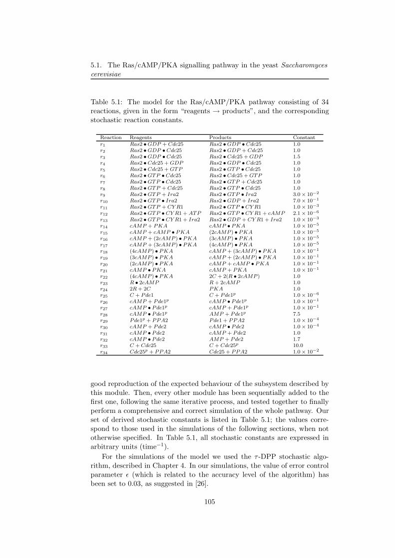
5.1. The Ras/cAMP/PKA signalling pathway in the yeast Saccharomycescerevisiae
Table 5.1: The model for the Ras/cAMP/PKA pathway consisting of 34reactions, given in the form “reagents → products”, and the correspondingstochastic reaction constants.
Reaction Reagents Products Constantr1 Ras2 • GDP + Cdc25 Ras2 • GDP • Cdc25 1.0r2 Ras2 • GDP • Cdc25 Ras2 • GDP + Cdc25 1.0r3 Ras2 • GDP • Cdc25 Ras2 • Cdc25 + GDP 1.5r4 Ras2 • Cdc25 + GDP Ras2 • GDP • Cdc25 1.0r5 Ras2 • Cdc25 + GTP Ras2 • GTP • Cdc25 1.0r6 Ras2 • GTP • Cdc25 Ras2 • Cdc25 + GTP 1.0r7 Ras2 • GTP • Cdc25 Ras2 • GTP + Cdc25 1.0r8 Ras2 • GTP + Cdc25 Ras2 • GTP • Cdc25 1.0r9 Ras2 • GTP + Ira2 Ras2 • GTP • Ira2 3.0 × 10⁻²
r10 Ras2 • GTP • Ira2 Ras2 • GDP + Ira2 7.0 × 10⁻¹
r11 Ras2 • GTP + CY R1 Ras2 • GTP • CY R1 1.0 × 10⁻³
r12 Ras2 • GTP • CY R1 + ATP Ras2 • GTP • CY R1 + cAMP 2.1 × 10⁻⁶
r13 Ras2 • GTP • CY R1 + Ira2 Ras2 • GDP + CY R1 + Ira2 1.0 × 10⁻³
r14 cAMP + PKA cAMP • PKA 1.0 × 10⁻⁵
r15 cAMP + cAMP • PKA (2cAMP ) • PKA 1.0 × 10⁻⁵
r16 cAMP + (2cAMP ) • PKA (3cAMP ) • PKA 1.0 × 10⁻⁵
r17 cAMP + (3cAMP ) • PKA (4cAMP ) • PKA 1.0 × 10⁻⁵
r18 (4cAMP ) • PKA cAMP + (3cAMP ) • PKA 1.0 × 10⁻¹
r19 (3cAMP ) • PKA cAMP + (2cAMP ) • PKA 1.0 × 10⁻¹
r20 (2cAMP ) • PKA cAMP + cAMP • PKA 1.0 × 10⁻¹
r21 cAMP • PKA cAMP + PKA 1.0 × 10⁻¹
r22 (4cAMP ) • PKA 2C + 2(R • 2cAMP ) 1.0r23 R • 2cAMP R + 2cAMP 1.0r24 2R + 2C PKA 1.0r25 C + Pde1 C + Pde1p 1.0 × 10⁻⁶
r26 cAMP + Pde1p cAMP • Pde1p 1.0 × 10⁻¹
r27 cAMP • Pde1p cAMP + Pde1p 1.0 × 10⁻¹
r28 cAMP • Pde1p AMP + Pde1p 7.5r29 Pde1p + PPA2 Pde1 + PPA2 1.0 × 10⁻⁴
r30 cAMP + Pde2 cAMP • Pde2 1.0 × 10⁻⁴
r31 cAMP • Pde2 cAMP + Pde2 1.0r32 cAMP • Pde2 AMP + Pde2 1.7r33 C + Cdc25 C + Cdc25p 10.0r34 Cdc25p + PPA2 Cdc25 + PPA2 1.0 × 10⁻²
good reproduction of the expected behaviour of the subsystem described bythis module. Then, every other module has been sequentially added to thefirst one, following the same iterative process, and tested together to finallyperform a comprehensive and correct simulation of the whole pathway. Ourset of derived stochastic constants is listed in Table 5.1; the values corre-spond to those used in the simulations of the following sections, when nototherwise specified. In Table 5.1, all stochastic constants are expressed inarbitrary units (time−1).
For the simulations of the model we used the τ -DPP stochastic algo-rithm, described in Chapter 4. In our simulations, the value of error controlparameter ǫ (which is related to the accuracy level of the algorithm) hasbeen set to 0.03, as suggested in [26].
105
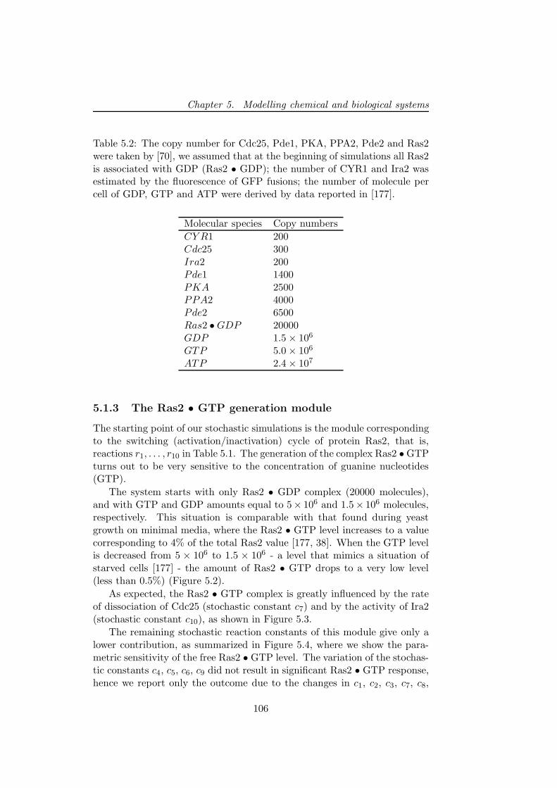
Chapter 5. Modelling chemical and biological systems
Table 5.2: The copy number for Cdc25, Pde1, PKA, PPA2, Pde2 and Ras2were taken by [70], we assumed that at the beginning of simulations all Ras2is associated with GDP (Ras2 • GDP); the number of CYR1 and Ira2 wasestimated by the fluorescence of GFP fusions; the number of molecule percell of GDP, GTP and ATP were derived by data reported in [177].
Molecular species Copy numbers
CY R1 200Cdc25 300Ira2 200Pde1 1400PKA 2500PPA2 4000Pde2 6500Ras2 • GDP 20000GDP 1.5 × 10⁶
GTP 5.0 × 10⁶
ATP 2.4 × 10⁷
5.1.3 The Ras2 • GTP generation module
The starting point of our stochastic simulations is the module correspondingto the switching (activation/inactivation) cycle of protein Ras2, that is,reactions r1, . . . , r10 in Table 5.1. The generation of the complex Ras2 • GTPturns out to be very sensitive to the concentration of guanine nucleotides(GTP).
The system starts with only Ras2 • GDP complex (20000 molecules),and with GTP and GDP amounts equal to 5× 10⁶ and 1.5× 10⁶ molecules,respectively. This situation is comparable with that found during yeastgrowth on minimal media, where the Ras2 • GTP level increases to a valuecorresponding to 4% of the total Ras2 value [177, 38]. When the GTP levelis decreased from 5 × 10⁶ to 1.5 × 10⁶ - a level that mimics a situation ofstarved cells [177] - the amount of Ras2 • GTP drops to a very low level(less than 0.5%) (Figure 5.2).
As expected, the Ras2 • GTP complex is greatly influenced by the rateof dissociation of Cdc25 (stochastic constant c7) and by the activity of Ira2(stochastic constant c10), as shown in Figure 5.3.
The remaining stochastic reaction constants of this module give only alower contribution, as summarized in Figure 5.4, where we show the para-metric sensitivity of the free Ras2 • GTP level. The variation of the stochas-tic constants c4, c5, c6, c9 did not result in significant Ras2 • GTP response,hence we report only the outcome due to the changes in c1, c2, c3, c7, c8,
106
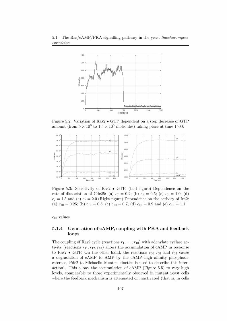
5.1. The Ras/cAMP/PKA signalling pathway in the yeast Saccharomycescerevisiae
0
200
400
600
800
1000
1200
1400
0 500 1000 1500 2000 2500 3000
Mole
cule
s
Time [a.u.]
Figure 5.2: Variation of Ras2 • GTP dependent on a step decrease of GTPamount (from 5 × 10⁶ to 1.5 × 10⁶ molecules) taking place at time 1500.
0.0 100
1.0 103
2.0 103
3.0 103
4.0 103
5.0 103
6.0 103
7.0 103
8.0 103
0 200 400 600 800 1000 1200 1400
Mole
cule
s
Time [a.u.]
(a) (b)
(c)
(d)
(e)
0.0 100
2.0 103
4.0 103
6.0 103
8.0 103
1.0 104
1.2 104
0 200 400 600 800 1000 1200 1400
Mole
cule
s
Time [a.u.]
(e)(d)
(c)
(b)
(a)
Figure 5.3: Sensitivity of Ras2 • GTP. (Left figure) Dependence on therate of dissociation of Cdc25: (a) c7 = 0.2; (b) c7 = 0.5; (c) c7 = 1.0; (d)c7 = 1.5 and (e) c7 = 2.0.(Right figure) Dependence on the activity of Ira2:(a) c10 = 0.25; (b) c10 = 0.5; (c) c10 = 0.7; (d) c10 = 0.9 and (e) c10 = 1.1.
c10 values.
5.1.4 Generation of cAMP, coupling with PKA and feedbackloops
The coupling of Ras2 cycle (reactions r1, . . . , r10) with adenylate cyclase ac-tivity (reactions r11, r12, r13) allows the accumulation of cAMP in responseto Ras2 • GTP. On the other hand, the reactions r30, r31 and r32 causea degradation of cAMP to AMP by the cAMP–high–affinity phosphodi-esterase, Pde2 (a Michaelis–Menten kinetics is used to describe this inter-action). This allows the accumulation of cAMP (Figure 5.5) to very highlevels, comparable to those experimentally observed in mutant yeast cellswhere the feedback mechanism is attenuated or inactivated (that is, in cells
107
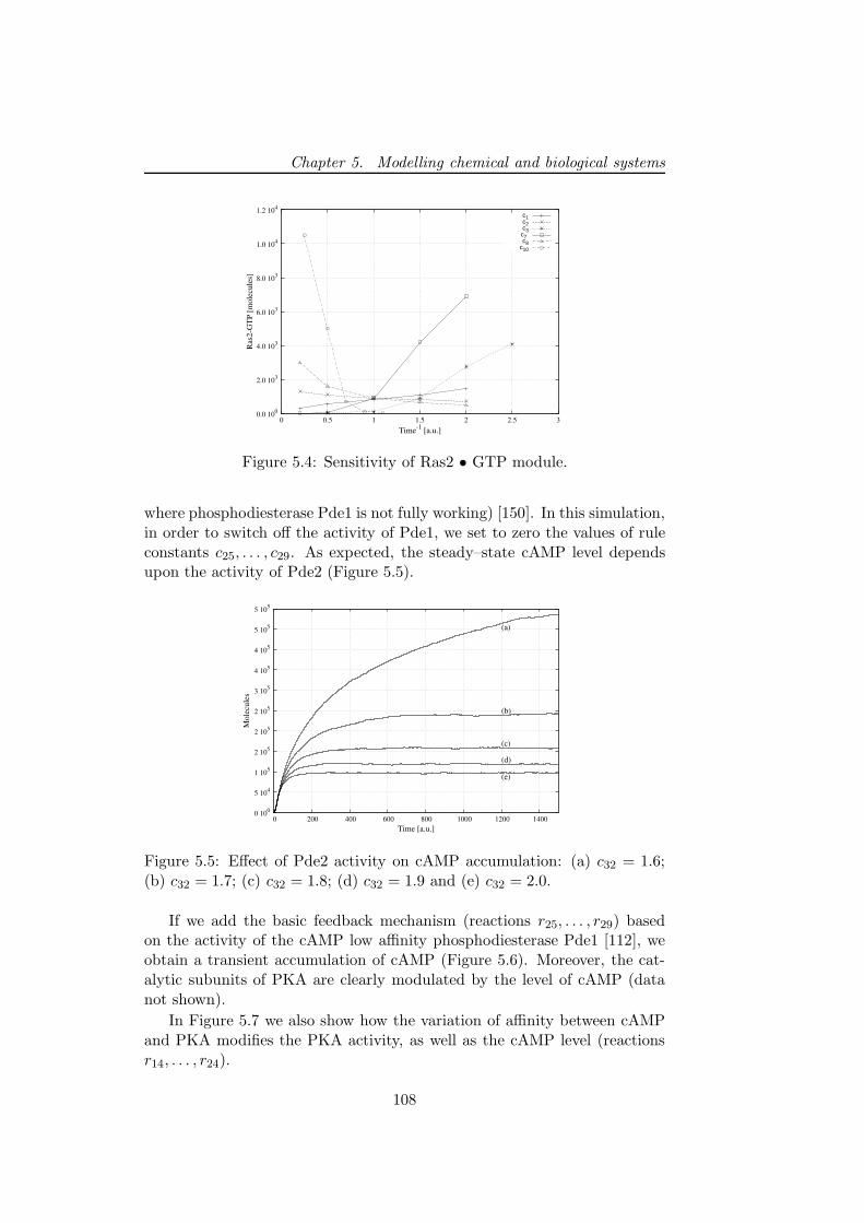
Chapter 5. Modelling chemical and biological systems
0.0 100
2.0 103
4.0 103
6.0 103
8.0 103
1.0 104
1.2 104
0 0.5 1 1.5 2 2.5 3
Ras2
-GT
P [
mole
cule
s]
Time-1
[a.u.]
c1c2c3c7 c8
c10
Figure 5.4: Sensitivity of Ras2 • GTP module.
where phosphodiesterase Pde1 is not fully working) [150]. In this simulation,in order to switch off the activity of Pde1, we set to zero the values of ruleconstants c25, . . . , c29. As expected, the steady–state cAMP level dependsupon the activity of Pde2 (Figure 5.5).
0 100
5 104
1 105
2 105
2 105
2 105
3 105
4 105
4 105
5 105
5 105
0 200 400 600 800 1000 1200 1400
Mole
cule
s
Time [a.u.]
(a)
(b)
(c)
(d)
(e)
Figure 5.5: Effect of Pde2 activity on cAMP accumulation: (a) c32 = 1.6;(b) c32 = 1.7; (c) c32 = 1.8; (d) c32 = 1.9 and (e) c32 = 2.0.
If we add the basic feedback mechanism (reactions r25, . . . , r29) basedon the activity of the cAMP low affinity phosphodiesterase Pde1 [112], weobtain a transient accumulation of cAMP (Figure 5.6). Moreover, the cat-alytic subunits of PKA are clearly modulated by the level of cAMP (datanot shown).
In Figure 5.7 we also show how the variation of affinity between cAMPand PKA modifies the PKA activity, as well as the cAMP level (reactionsr14, . . . , r24).
108
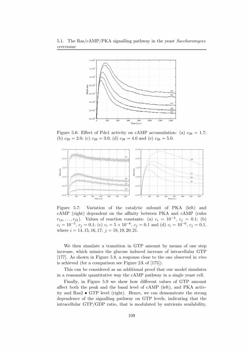
5.1. The Ras/cAMP/PKA signalling pathway in the yeast Saccharomycescerevisiae
0.0 100
2.0 104
4.0 104
6.0 104
8.0 104
1.0 105
1.2 105
1.4 105
0 200 400 600 800 1000 1200 1400
Mole
cule
s
Time [a.u.]
(e)
(d)
(c)
(b)
(a)
Figure 5.6: Effect of Pde1 activity on cAMP accumulation: (a) c28 = 1.7;(b) c28 = 2.0; (c) c28 = 3.0; (d) c28 = 4.0 and (e) c28 = 5.0.
0.0 100
5.0 102
1.0 103
1.5 103
2.0 103
2.5 103
0 200 400 600 800 1000 1200 1400
Mole
cule
s
Time [a.u.]
(d)
(c)
(b)
(a)
0.0 100
5.0 104
1.0 105
1.5 105
2.0 105
2.5 105
0 200 400 600 800 1000 1200 1400
Mole
cule
s
Time [a.u.]
(a)
(b)
(c)
(d)
Figure 5.7: Variation of the catalytic subunit of PKA (left) andcAMP (right) dependent on the affinity between PKA and cAMP (rulesr14, . . . , r21). Values of reaction constants: (a) ci = 10−4, cj = 0.1; (b)ci = 10−5, cj = 0.1; (c) ci = 5 × 10⁻⁶, cj = 0.1 and (d) ci = 10−6, cj = 0.1,where i = 14, 15, 16, 17; j = 18, 19, 20, 21.
We then simulate a transition in GTP amount by means of one stepincrease, which mimics the glucose induced increase of intracellular GTP[177]. As shown in Figure 5.8, a response close to the one observed in vivois achieved (for a comparison see Figure 2A of [175]).
This can be considered as an additional proof that our model simulatesin a reasonable quantitative way the cAMP pathway in a single yeast cell.
Finally, in Figure 5.9 we show how different values of GTP amountaffect both the peak and the basal level of cAMP (left), and PKA activ-ity and Ras2 • GTP level (right). Hence, we can demonstrate the strongdependence of the signalling pathway on GTP levels, indicating that theintracellular GTP/GDP ratio, that is modulated by nutrients availability,
109
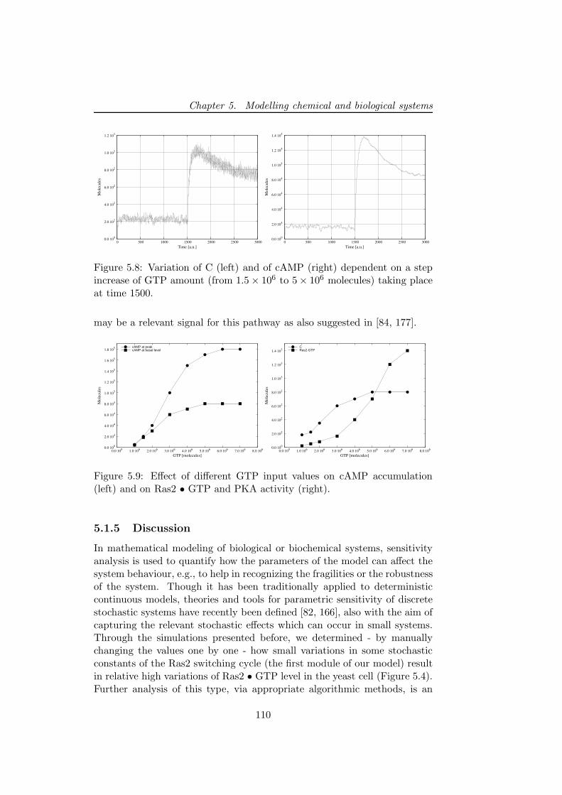
Chapter 5. Modelling chemical and biological systems
0.0 100
2.0 102
4.0 102
6.0 102
8.0 102
1.0 103
1.2 103
0 500 1000 1500 2000 2500 3000
Mole
cule
s
Time [a.u.]
0.0 100
2.0 104
4.0 104
6.0 104
8.0 104
1.0 105
1.2 105
1.4 105
0 500 1000 1500 2000 2500 3000
Mole
cule
s
Time [a.u.]
Figure 5.8: Variation of C (left) and of cAMP (right) dependent on a stepincrease of GTP amount (from 1.5 × 10⁶ to 5× 10⁶ molecules) taking placeat time 1500.
may be a relevant signal for this pathway as also suggested in [84, 177].
0.0 100
2.0 104
4.0 104
6.0 104
8.0 104
1.0 105
1.2 105
1.4 105
1.6 105
1.8 105
0.0 100
1.0 106
2.0 106
3.0 106
4.0 106
5.0 106
6.0 106
7.0 106
8.0 106
Mole
cule
s
GTP [molecules]
cAMP at peakcAMP at basal level
0.0 100
2.0 102
4.0 102
6.0 102
8.0 102
1.0 103
1.2 103
1.4 103
0.0 100
1.0 106
2.0 106
3.0 106
4.0 106
5.0 106
6.0 106
7.0 106
8.0 106
Mole
cule
s
GTP [molecules]
CRas2-GTP
Figure 5.9: Effect of different GTP input values on cAMP accumulation(left) and on Ras2 • GTP and PKA activity (right).
5.1.5 Discussion
In mathematical modeling of biological or biochemical systems, sensitivityanalysis is used to quantify how the parameters of the model can affect thesystem behaviour, e.g., to help in recognizing the fragilities or the robustnessof the system. Though it has been traditionally applied to deterministiccontinuous models, theories and tools for parametric sensitivity of discretestochastic systems have recently been defined [82, 166], also with the aim ofcapturing the relevant stochastic effects which can occur in small systems.Through the simulations presented before, we determined - by manuallychanging the values one by one - how small variations in some stochasticconstants of the Ras2 switching cycle (the first module of our model) resultin relative high variations of Ras2 • GTP level in the yeast cell (Figure 5.4).Further analysis of this type, via appropriate algorithmic methods, is an
110
5.1. The Ras/cAMP/PKA signalling pathway in the yeast Saccharomycescerevisiae
ongoing work and will be elaborated for the whole pathway.Indeed, a crucial point in understanding the dynamics of biological sys-
tems through computer simulations is related to the evaluation of the pa-rameters involved in the system, such as molecular concentrations (or copynumbers), binding constants, transcription or translation rates, etc. Exceptfor few special cases where the values can be found in literature, these con-stants are not available or else ambiguous. The lack of information and theinaccuracy about these data are often due to the difficulty, or the impossi-bility, to perform correct measures during in vivo or in vitro experiments.
This fact then results in the challenging problem of assigning a reasonabletemporal dimension to the (stochastic) simulation results. The problem ofcalibrating the system’s parameters can be tackled by using optimisationtechniques in order to find a set of optimal parameter values which canbe used to reproduce the observed dynamics of a system, as explained inChapter 6.
For the simulations of the Ras/cAMP/PKA pathway, we were able tomake a direct comparison between the simulations and the experimentalresults. In yeast, cAMP was experimentally found to be around 2 × 10⁵
molecules after stimulation, while basal levels were around 2-5 × 10⁴ mole-cules/cell. In addition, after stimulation, a cAMP peak was observed after45-60 s, then a decrease was observed and a new steady–state reached in3-5 min (for a direct comparison see the paper [175], Figure 2). Theseexperimental data fit very well with our stochastic simulations, hence, weare in the condition to assign a reasonable temporal scale to our simulations.A similar quantitative comparison can be done for Ras2 • GTP, which wasexperimentally found to be in the range of 2-4% of total Ras2 in growingcells (equivalent to 400-800 molecules/cell).
In addition, after stimulation of starved cells with glucose, Ras2 • GTPincreased from 0.5 to 4% of total Ras2 in about 1 min [177], and again thesedata fit very well with our simulations.
In this work, we focused on the cytoplasmic regulators of the Ras/-cAMP/PKA pathway, and provided stochastic simulations of the synthesisof cAMP and of the cytoplasmic quantities of the pivotal complexes. As afuture development, we will construct an accurate map of related cellularphenomena, such as the response of this pathway to nutrients and to in-tracellular acidification, its connections with other pathways co–involved inglucose signalling, and the downhill nuclear expression of target genes. Here,we have used the level of intracellular GTP as input, that was experimen-tally found to quickly respond to nutrients availability [177], but we couldalso simulate the effect of a decrease of intracellular pH (that likely causesan inhibition of GAP activity of the Ira proteins [37], or a fast increase ofCdc25 activity [38]). In order to gain a higher biological relevance of ourmodel, we will include the Gpr1/Gpa2 pathway, which is a specific signallingmechanism that responds only to high glucose concentration, and operates
111
Chapter 5. Modelling chemical and biological systems
together with Ras2 • GTP to activate adenylate cyclase [37, 175]. Finally,we will also test the effect of additional feedback mechanisms, such as theinactivation of Cdc25, the activation of Ira, etc.
We also expect that our computational studies will support the experi-mental work aimed at characterizing the actual localizations (that is, eitherbound to plasma membrane or to internal membranes, or diffused withinthe cell) of the central components of this pathway, since there exists evi-dence that most of the Cdc25, CYR1, Ira2, Ras2 proteins localize in internalmembranes, suggesting the presence of large signalling complexes inside theyeast cells [119].
The τ -DPP algorithm [30, 118] will be exploited in order to investigatethe topological distribution of the molecular species in distinct cellular re-gions, and to introduce additional components and other external inputs.
Finally, we believe that establishing the pivotal roles of the differentcomponents in the Ras/cAMP/PKA pathway in yeast might have a posi-tive outcome for the elucidation of similar components in higher eukaryotes.For instance, it is well known that the protein neurofibromin 1 (NF1), act-ing as tumor suppressor in human cells, is homologous to the proteins of theIra family, and it has been shown to contain a GAP related domain whichregulates Ras [10]. Though its evident importance, biochemical and cellularcharacterizations of NF1 are still on the way, and very few knowledge is cur-rently available about NF1-interacting proteins. Therefore, the synergisticintegration of pathway modeling and of deletion experiments about Ira pro-teins in yeast could probably provide useful hints for further interdisciplinaryinvestigations of NF1.
112
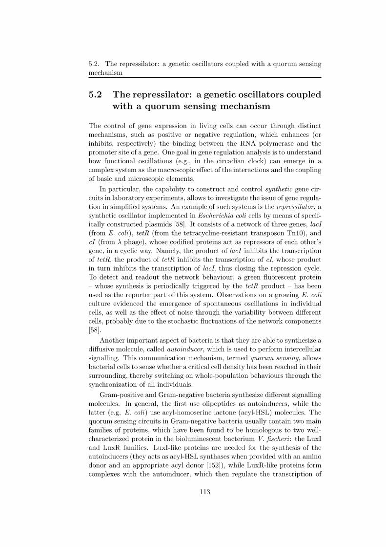
5.2. The repressilator: a genetic oscillators coupled with a quorum sensingmechanism
5.2 The repressilator: a genetic oscillators coupledwith a quorum sensing mechanism
The control of gene expression in living cells can occur through distinctmechanisms, such as positive or negative regulation, which enhances (orinhibits, respectively) the binding between the RNA polymerase and thepromoter site of a gene. One goal in gene regulation analysis is to understandhow functional oscillations (e.g., in the circadian clock) can emerge in acomplex system as the macroscopic effect of the interactions and the couplingof basic and microscopic elements.
In particular, the capability to construct and control synthetic gene cir-cuits in laboratory experiments, allows to investigate the issue of gene regula-tion in simplified systems. An example of such systems is the repressilator, asynthetic oscillator implemented in Escherichia coli cells by means of specif-ically constructed plasmids [58]. It consists of a network of three genes, lacI(from E. coli), tetR (from the tetracycline-resistant transposon Tn10), andcI (from λ phage), whose codified proteins act as repressors of each other’sgene, in a cyclic way. Namely, the product of lacI inhibits the transcriptionof tetR, the product of tetR inhibits the transcription of cI, whose productin turn inhibits the transcription of lacI, thus closing the repression cycle.To detect and readout the network behaviour, a green fluorescent protein– whose synthesis is periodically triggered by the tetR product – has beenused as the reporter part of this system. Observations on a growing E. coliculture evidenced the emergence of spontaneous oscillations in individualcells, as well as the effect of noise through the variability between differentcells, probably due to the stochastic fluctuations of the network components[58].
Another important aspect of bacteria is that they are able to synthesize adiffusive molecule, called autoinducer, which is used to perform intercellularsignalling. This communication mechanism, termed quorum sensing, allowsbacterial cells to sense whether a critical cell density has been reached in theirsurrounding, thereby switching on whole-population behaviours through thesynchronization of all individuals.
Gram-positive and Gram-negative bacteria synthesize different signallingmolecules. In general, the first use olipeptides as autoinducers, while thelatter (e.g. E. coli) use acyl-homoserine lactone (acyl-HSL) molecules. Thequorum sensing circuits in Gram-negative bacteria usually contain two mainfamilies of proteins, which have been found to be homologous to two well-characterized protein in the bioluminescent bacterium V. fischeri : the LuxIand LuxR families. LuxI-like proteins are needed for the synthesis of theautoinducers (they acts as acyl-HSL synthases when provided with an aminodonor and an appropriate acyl donor [152]), while LuxR-like proteins formcomplexes with the autoinducer, which then regulate the transcription of
113
Chapter 5. Modelling chemical and biological systems
target genes [132].
In [67], a synthetic multicellular clock has been investigated, by couplingthe repressilator system with bacterial quorum sensing. This intercellularcommunication mechanism is able to lead the local genetic oscillators, withina noisy and nonidentical population, to global oscillatory rhythms. In partic-ular, it was shown that individual repressilator systems can self-synchronize,even when their periods are broadly distributed [67].
In this section, we propose a multivolume model based on τ -DPP thatconsiders a repressilator-like system (RL) coupled with a quorum sensing-like circuit (QSL). Namely, the RL consists of three genes (G1, G2, G3) whichcyclically inhibit each other’s expression, while the QSL consists of a geneticcomponent that triggers the production of the autoinducer (through the syn-thesis of the intermediate autoinducer-synthases), plus a “control” moleculethat mimics the role of the protein in the LuxR family. The two systems areinterlaced through one positive feedback and one negative feedforward loop:the first operates on the promotion of gene G1 in the RL by means of theQSL autoinducer molecule, while the second operates on the inhibition ofthe QSL gene by means of G1 product (see Figure 5.10).
Figure 5.10: The (single volume) network of the genetic oscillator systemcoupled with quorum sensing mechanism.
5.2.1 A multivolume model for coupled genetic oscillators
The multivolume model for RL + QSL system consists of n volumes, eachone corresponding to a cell, a set of 34 reactions defined within each cell (Ta-ble 5.3), 1 communication reaction defined in the environment (Table 5.4),
114
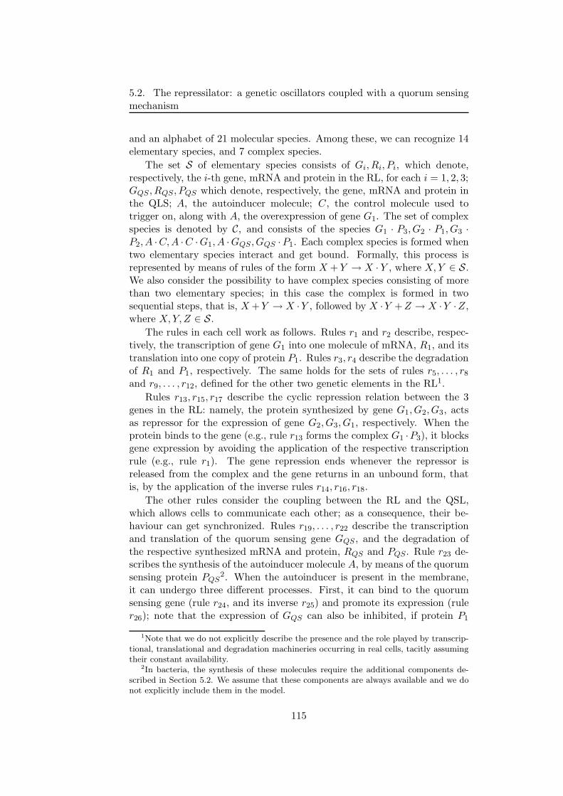
5.2. The repressilator: a genetic oscillators coupled with a quorum sensingmechanism
and an alphabet of 21 molecular species. Among these, we can recognize 14elementary species, and 7 complex species.
The set S of elementary species consists of Gi, Ri, Pi, which denote,respectively, the i-th gene, mRNA and protein in the RL, for each i = 1, 2, 3;GQS , RQS, PQS which denote, respectively, the gene, mRNA and protein inthe QLS; A, the autoinducer molecule; C, the control molecule used totrigger on, along with A, the overexpression of gene G1. The set of complexspecies is denoted by C, and consists of the species G1 · P3, G2 · P1, G3 ·P2, A ·C,A ·C ·G1, A ·GQS, GQS ·P1. Each complex species is formed whentwo elementary species interact and get bound. Formally, this process isrepresented by means of rules of the form X + Y → X · Y , where X,Y ∈ S.We also consider the possibility to have complex species consisting of morethan two elementary species; in this case the complex is formed in twosequential steps, that is, X +Y → X ·Y , followed by X ·Y +Z → X ·Y ·Z,where X,Y,Z ∈ S.
The rules in each cell work as follows. Rules r1 and r2 describe, respec-tively, the transcription of gene G1 into one molecule of mRNA, R1, and itstranslation into one copy of protein P1. Rules r3, r4 describe the degradationof R1 and P1, respectively. The same holds for the sets of rules r5, . . . , r8
and r9, . . . , r12, defined for the other two genetic elements in the RL1.
Rules r13, r15, r17 describe the cyclic repression relation between the 3genes in the RL: namely, the protein synthesized by gene G1, G2, G3, actsas repressor for the expression of gene G2, G3, G1, respectively. When theprotein binds to the gene (e.g., rule r13 forms the complex G1 ·P3), it blocksgene expression by avoiding the application of the respective transcriptionrule (e.g., rule r1). The gene repression ends whenever the repressor isreleased from the complex and the gene returns in an unbound form, thatis, by the application of the inverse rules r14, r16, r18.
The other rules consider the coupling between the RL and the QSL,which allows cells to communicate each other; as a consequence, their be-haviour can get synchronized. Rules r19, . . . , r22 describe the transcriptionand translation of the quorum sensing gene GQS , and the degradation ofthe respective synthesized mRNA and protein, RQS and PQS. Rule r23 de-scribes the synthesis of the autoinducer molecule A, by means of the quorumsensing protein PQS
2. When the autoinducer is present in the membrane,it can undergo three different processes. First, it can bind to the quorumsensing gene (rule r24, and its inverse r25) and promote its expression (ruler26); note that the expression of GQS can also be inhibited, if protein P1
1Note that we do not explicitly describe the presence and the role played by transcrip-tional, translational and degradation machineries occurring in real cells, tacitly assumingtheir constant availability.
2In bacteria, the synthesis of these molecules require the additional components de-scribed in Section 5.2. We assume that these components are always available and we donot explicitly include them in the model.
115
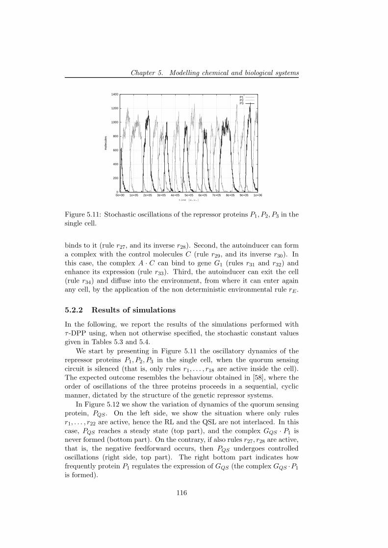
Chapter 5. Modelling chemical and biological systems
0
200
400
600
800
1000
1200
1400
0e+00 1e+05 2e+05 3e+05 4e+05 5e+05 6e+05 7e+05 8e+05 9e+05 1e+06
mol
ecul
es
time [a.u.]
P1P2P3
Figure 5.11: Stochastic oscillations of the repressor proteins P1, P2, P3 in thesingle cell.
binds to it (rule r27, and its inverse r28). Second, the autoinducer can forma complex with the control molecules C (rule r29, and its inverse r30). Inthis case, the complex A · C can bind to gene G1 (rules r31 and r32) andenhance its expression (rule r33). Third, the autoinducer can exit the cell(rule r34) and diffuse into the environment, from where it can enter againany cell, by the application of the non deterministic environmental rule rE.
5.2.2 Results of simulations
In the following, we report the results of the simulations performed withτ -DPP using, when not otherwise specified, the stochastic constant valuesgiven in Tables 5.3 and 5.4.
We start by presenting in Figure 5.11 the oscillatory dynamics of therepressor proteins P1, P2, P3 in the single cell, when the quorum sensingcircuit is silenced (that is, only rules r1, . . . , r18 are active inside the cell).The expected outcome resembles the behaviour obtained in [58], where theorder of oscillations of the three proteins proceeds in a sequential, cyclicmanner, dictated by the structure of the genetic repressor systems.
In Figure 5.12 we show the variation of dynamics of the quorum sensingprotein, PQS. On the left side, we show the situation where only rulesr1, . . . , r22 are active, hence the RL and the QSL are not interlaced. In thiscase, PQS reaches a steady state (top part), and the complex GQS · P1 isnever formed (bottom part). On the contrary, if also rules r27, r28 are active,that is, the negative feedforward occurs, then PQS undergoes controlledoscillations (right side, top part). The right bottom part indicates howfrequently protein P1 regulates the expression of GQS (the complex GQS ·P1
is formed).
116
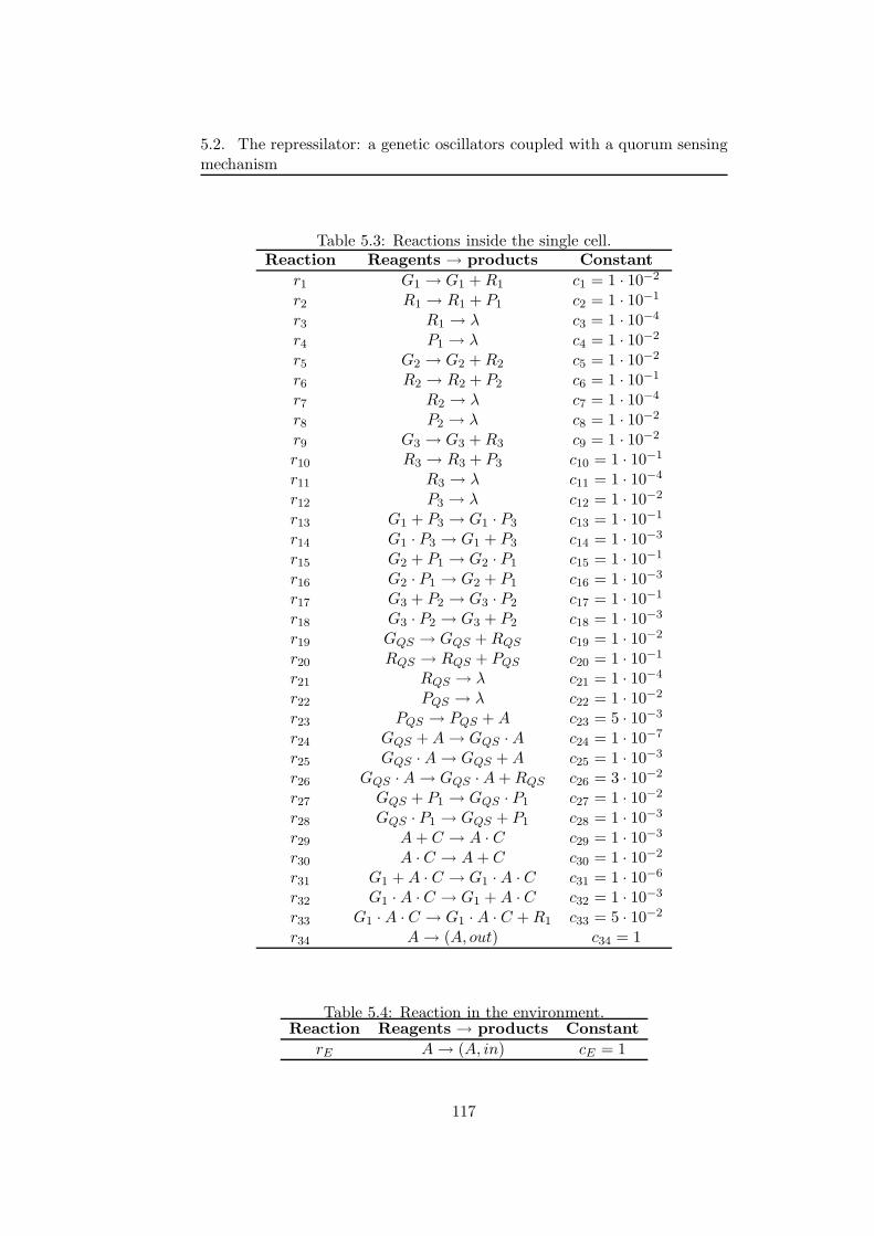
5.2. The repressilator: a genetic oscillators coupled with a quorum sensingmechanism
Table 5.3: Reactions inside the single cell.Reaction Reagents → products Constant
r1 G1 → G1 + R1 c1 = 1 · 10−2
r2 R1 → R1 + P1 c2 = 1 · 10−1
r3 R1 → λ c3 = 1 · 10−4
r4 P1 → λ c4 = 1 · 10−2
r5 G2 → G2 + R2 c5 = 1 · 10−2
r6 R2 → R2 + P2 c6 = 1 · 10−1
r7 R2 → λ c7 = 1 · 10−4
r8 P2 → λ c8 = 1 · 10−2
r9 G3 → G3 + R3 c9 = 1 · 10−2
r10 R3 → R3 + P3 c10 = 1 · 10−1
r11 R3 → λ c11 = 1 · 10−4
r12 P3 → λ c12 = 1 · 10−2
r13 G1 + P3 → G1 · P3 c13 = 1 · 10−1
r14 G1 · P3 → G1 + P3 c14 = 1 · 10−3
r15 G2 + P1 → G2 · P1 c15 = 1 · 10−1
r16 G2 · P1 → G2 + P1 c16 = 1 · 10−3
r17 G3 + P2 → G3 · P2 c17 = 1 · 10−1
r18 G3 · P2 → G3 + P2 c18 = 1 · 10−3
r19 GQS → GQS + RQS c19 = 1 · 10−2
r20 RQS → RQS + PQS c20 = 1 · 10−1
r21 RQS → λ c21 = 1 · 10−4
r22 PQS → λ c22 = 1 · 10−2
r23 PQS → PQS + A c23 = 5 · 10−3
r24 GQS + A → GQS · A c24 = 1 · 10−7
r25 GQS · A → GQS + A c25 = 1 · 10−3
r26 GQS · A → GQS · A + RQS c26 = 3 · 10−2
r27 GQS + P1 → GQS · P1 c27 = 1 · 10−2
r28 GQS · P1 → GQS + P1 c28 = 1 · 10−3
r29 A + C → A · C c29 = 1 · 10−3
r30 A · C → A + C c30 = 1 · 10−2
r31 G1 + A · C → G1 · A · C c31 = 1 · 10−6
r32 G1 · A · C → G1 + A · C c32 = 1 · 10−3
r33 G1 · A · C → G1 · A · C + R1 c33 = 5 · 10−2
r34 A → (A, out) c34 = 1
Table 5.4: Reaction in the environment.Reaction Reagents → products Constant
rE A → (A, in) cE = 1
117
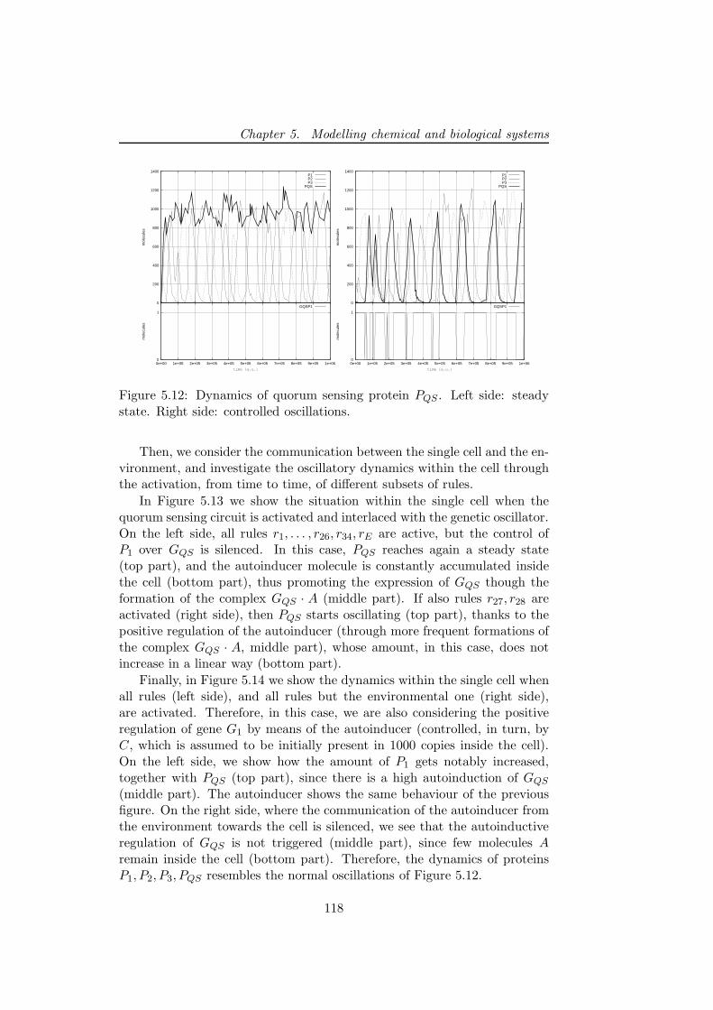
Chapter 5. Modelling chemical and biological systems
0
200
400
600
800
1000
1200
1400
mol
ecul
es
P1P2P3
PQS
0
1
0e+00 1e+05 2e+05 3e+05 4e+05 5e+05 6e+05 7e+05 8e+05 9e+05 1e+06
mol
ecul
es
time [a.u.]
GQSP1 0
200
400
600
800
1000
1200
1400
mol
ecul
es
P1P2P3
PQS
0
1
0e+00 1e+05 2e+05 3e+05 4e+05 5e+05 6e+05 7e+05 8e+05 9e+05 1e+06
mol
ecul
es
time [a.u.]
GQSP1
Figure 5.12: Dynamics of quorum sensing protein PQS . Left side: steadystate. Right side: controlled oscillations.
Then, we consider the communication between the single cell and the en-vironment, and investigate the oscillatory dynamics within the cell throughthe activation, from time to time, of different subsets of rules.
In Figure 5.13 we show the situation within the single cell when thequorum sensing circuit is activated and interlaced with the genetic oscillator.On the left side, all rules r1, . . . , r26, r34, rE are active, but the control ofP1 over GQS is silenced. In this case, PQS reaches again a steady state(top part), and the autoinducer molecule is constantly accumulated insidethe cell (bottom part), thus promoting the expression of GQS though theformation of the complex GQS · A (middle part). If also rules r27, r28 areactivated (right side), then PQS starts oscillating (top part), thanks to thepositive regulation of the autoinducer (through more frequent formations ofthe complex GQS · A, middle part), whose amount, in this case, does notincrease in a linear way (bottom part).
Finally, in Figure 5.14 we show the dynamics within the single cell whenall rules (left side), and all rules but the environmental one (right side),are activated. Therefore, in this case, we are also considering the positiveregulation of gene G1 by means of the autoinducer (controlled, in turn, byC, which is assumed to be initially present in 1000 copies inside the cell).On the left side, we show how the amount of P1 gets notably increased,together with PQS (top part), since there is a high autoinduction of GQS
(middle part). The autoinducer shows the same behaviour of the previousfigure. On the right side, where the communication of the autoinducer fromthe environment towards the cell is silenced, we see that the autoinductiveregulation of GQS is not triggered (middle part), since few molecules Aremain inside the cell (bottom part). Therefore, the dynamics of proteinsP1, P2, P3, PQS resembles the normal oscillations of Figure 5.12.
118
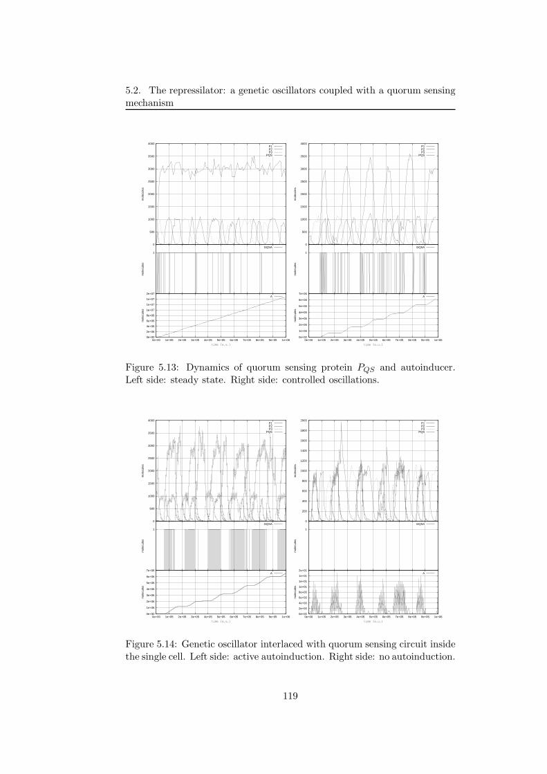
5.2. The repressilator: a genetic oscillators coupled with a quorum sensingmechanism
0
500
1000
1500
2000
2500
3000
3500
4000m
olec
ules
P1P2P3
PQS
1
mol
ecul
es
GQSA
0e+00
2e+06
4e+06
6e+06
8e+06
1e+07
1e+07
1e+07
2e+07
0e+00 1e+05 2e+05 3e+05 4e+05 5e+05 6e+05 7e+05 8e+05 9e+05 1e+06
mol
ecul
es
time [a.u.]
A
0
500
1000
1500
2000
2500
3000
3500
4000
mol
ecul
es
P1P2P3
PQS
1
mol
ecul
es
GQSA
0e+00
1e+06
2e+06
3e+06
4e+06
5e+06
6e+06
7e+06
0e+00 1e+05 2e+05 3e+05 4e+05 5e+05 6e+05 7e+05 8e+05 9e+05 1e+06
mol
ecul
es
time [a.u.]
A
Figure 5.13: Dynamics of quorum sensing protein PQS and autoinducer.Left side: steady state. Right side: controlled oscillations.
0
500
1000
1500
2000
2500
3000
3500
4000
mol
ecul
es
P1P2P3
PQS
1
mol
ecul
es
GQSA
0e+00
1e+06
2e+06
3e+06
4e+06
5e+06
6e+06
7e+06
0e+00 1e+05 2e+05 3e+05 4e+05 5e+05 6e+05 7e+05 8e+05 9e+05 1e+06
mol
ecul
es
time [a.u.]
A
0
200
400
600
800
1000
1200
1400
1600
1800
2000
mol
ecul
es
P1P2P3
PQS
1
mol
ecul
es
GQSA
0e+00
2e+00
4e+00
6e+00
8e+00
1e+01
1e+01
1e+01
2e+01
0e+00 1e+05 2e+05 3e+05 4e+05 5e+05 6e+05 7e+05 8e+05 9e+05 1e+06
mol
ecul
es
time [a.u.]
A
Figure 5.14: Genetic oscillator interlaced with quorum sensing circuit insidethe single cell. Left side: active autoinduction. Right side: no autoinduction.
119
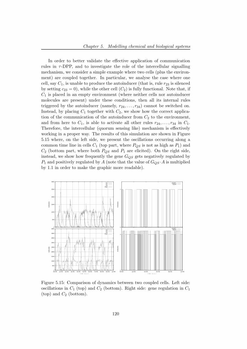
Chapter 5. Modelling chemical and biological systems
In order to better validate the effective application of communicationrules in τ -DPP, and to investigate the role of the intercellular signallingmechanism, we consider a simple example where two cells (plus the environ-ment) are coupled together. In particular, we analyse the case where onecell, say C1, is unable to produce the autoinducer (that is, rule r23 is silencedby setting c23 = 0), while the other cell (C2) is fully functional. Note that, ifC1 is placed in an empty environment (where neither cells nor autoinducermolecules are present) under these conditions, then all its internal rulestriggered by the autoinducer (namely, r24, . . . , r34) cannot be switched on.Instead, by placing C1 together with C2, we show how the correct applica-tion of the communication of the autoinducer from C2 to the environment,and from here to C1, is able to activate all other rules r24, . . . , r34 in C1.Therefore, the intercellular (quorum sensing like) mechanism is effectivelyworking in a proper way. The results of this simulation are shown in Figure5.15 where, on the left side, we present the oscillations occurring along acommon time line in cells C1 (top part, where PQS is not as high as P1) andC2 (bottom part, where both PQS and P1 are elicited). On the right side,instead, we show how frequently the gene GQS gets negatively regulated byP1 and positively regulated by A (note that the value of GQS ·A is multipliedby 1.1 in order to make the graphic more readable).
0
500
1000
1500
2000
2500
3000
mol
ecul
es
P1P2P3
PQS
0
500
1000
1500
2000
2500
3000
3500
4000
4500
0e+00 1e+05 2e+05 3e+05 4e+05 5e+05 6e+05 7e+05 8e+05 9e+05 1e+06
mol
ecul
es
time [a.u.]
P1P2P3
PQS
0
1
mol
ecul
es
GQSP1GQSA
0
1
0e+00 2e+05 4e+05 6e+05 8e+05 1e+06
mol
ecul
es
time [a.u.]
GQSP1GQSA
Figure 5.15: Comparison of dynamics between two coupled cells. Left side:oscillations in C1 (top) and C2 (bottom). Right side: gene regulation in C1
(top) and C2 (bottom).
120
5.2. The repressilator: a genetic oscillators coupled with a quorum sensingmechanism
5.2.3 Discussion and future developments
The investigation of this system allows us to make some considerations onone of the key issues that are related to the simulation of biological systemsby means of τ -DPP, that is, the role of stochastic constants associated withcommunication rules. Usually, in τ -DPP application of a communicationrule means that an object (or a set of objects) is instantaneously sent to thetarget volume, without considering the “time” that the objects could needto move from one volume to another one. For instance, a communicationrule might represent the passage of a solute through a cellular membranemediated by a transport protein. This biological process can require a con-formational change in the transport protein structure, which necessarilyprolong the time the solute would take to virtually cross the membrane in adirect way [146]. Since in τ -DPP we are not considering intermediate “pas-sage structures”, a tuning of the stochastic constants of the communicationrules is necessary, in order to better represent the behaviour of the objectsthat move between adjacent volumes.
Furthermore, it would be interesting to check whether a more complexsystem, consisting of a population of many coupled cells, can show (emer-gent) synchronization events with respect to the oscillations of the threerepressor proteins and the quorum sensing protein. Since the modelling andsimulation approach we use here is stochastic, the gain of such a synchro-nized behaviour in a noisy system is harder than doing this with a deter-ministic approach (see, e.g., [67]). We will deal with this issue in a futuredevelopment of this work.
Another extension of this work might consist in considering more com-plex systems, with populations of different kind of bacteria which oscillateaccording to a predator–prey dynamics. An example of such kind of systemshas been introduced in [9], where the authors presented a synthetic ecosys-tem composed by two (different) E. coli populations, able to communicateby means of a quorum sensing mechanism. In particular, the interactionsbetween the two species regulate each other’s gene expression and survival.Indeed, the predator bacteria can kill the prey by inducing the expressionof a killer protein in the prey, while preys save predators from committing“suicide” by eliciting the expression of an antidote protein in the predators.
These features might be considered also in a more structured system, i.e.a metapopulation (see Section 3.3), in order to investigate the different dy-namics of the bacterial populations with respect to the topological structureof the environment where they interact.
121
Chapter 5. Modelling chemical and biological systems
5.3 First steps toward a wet implementation forτ-DPP
The aim of this section is to propose a correspondence between τ -DPP andchemical reacting systems occurring inside micro reactors. Micro reactors[87] are laboratory devices consisting of several reacting volumes (reactors)with a size at the scale of the µl, connected by channels used to transportmolecules. Indeed, there is a close relation between the topological descrip-tion of these two systems: they are both composed by several volumes, andamong these volumes it is possible to communicate molecules. Moreover,the approach based on multiset rewriting rules, that characterises τ -DPP,is similar to the chemical reacting process occurring within a micro reactor.Furthermore, both τ -DPP and chemical reacting systems emphasise the in-trinsic stochasticity of chemical processes. The “noise”, associated to thestochastic behaviour, rules the system dynamics at the micro-scales. At thisscale, the small volumes and the high dilutions result in a system whereparticles interaction should be described in a discrete fashion. Finally, thecommunication processes described by means of communication rules withinτ -DPP, are strictly related to the channels interconnecting the reactors.
In this section, we show how these analogies can be exploited to proposea feasible wet implementation of τ -DPP. To obtain a description of τ -DPPthat can be implemented using micro reactors in a straightforward way,we consider the encoding of boolean functions, Fredkin gates and circuitsthrough chemical reactions, following the chemical computing principles.
Chemical computing [49] is a technique used to process information bymeans of real molecules, modified by chemical reactions, or by using elec-tronic devices that are programmed following some principles coming fromchemistry. Moreover, in chemical computing, the result of a computation isrepresented by the emergent global behaviour, obtained from the applicationof small systems characterised by chemical reactions.
Exploiting the chemical organisation theory [122], we can define a chemi-cal network in order to describe a system as a collection of reactions appliedto a given set of molecular species. Moreover, we can identify the set of(so called) organisations, in the set of molecular species, to describe thebehaviour of such system. So doing, the behaviour is traced by means of“movement” between organisations.
Furthermore, a different kind of problem encoding will be presented,that is based on the instructions of register machines [134]. This approach issimilar to the one related to the chemical computing field. The idea is to usea set of chemical reactions to realize the instructions of the register machines.For instance, in Section 5.3.2, the formalisation and the simulation of adecrement instruction by means of τ -DPP, is presented.
122
5.3. First steps toward a wet implementation for τ -DPP
5.3.1 Chemical computing
Here we introduce the basic notions of chemical computing, a novel compu-tational paradigm where the information is processed by means of chemicalreactions. Then, we recall the basic definitions of chemical organisation the-ory, that can be used gain additional knowledge on a chemical computingsystem, such as its emergent behaviour.
In any generic biochemical system, information is processed by means ofchemical reactions occurring between “elementary” components (i.e. mole-cules); by exploiting this metaphor, chemical reactions can be used to builda novel computational paradigm [49]. This approach is called chemical com-puting, and it is related to the ways of performing computations with bothreal molecules and electronic devices, which are programmed using principlestaken from chemistry.
In general, the analysis of the outcome of chemical reaction processesis hard because of their nonlinearity. The same problems are related tothe analysis of biological systems, since the global behaviour can be verydifferent from behaviour of their local components.
In order to work out this problem, the notions of chemical organisationtheory can be used to analyse the emergent behaviour of the system, startingfrom its smaller components; so doing, it is possible to link the evolutiongoverned by the set of all single reactions to the global dynamics of thesystem.
Chemical organisation theory [122] is used to identify a hierarchy of selfmaintaining sub-networks, belonging to a chemical reaction network. Thesesub-networks are called organisations. In particular, a chemical organisa-tion is a set of molecular species that satisfies two properties, that is, it isalgebraically closed and stoichiometrically self-maintaining. Here we reportan informal definition of these concepts, and refer the reader to [122] forformal definitions and further details.
A reaction network is a tuple 〈M,R〉, where M is a set of molecularspecies and R is a set of reactions (also called rules). The rules in R aregiven by the relation R : PM(M)×PM(M), where PM(M) denotes the setof all the multisets of elements in M. The general form of a rule is α1m1 +α2m2 + · · · + αkmk → β1m1 + β2m2 + · · · + βkmk, where m1, . . . ,mk ∈ Mare the molecular species involved in the rule and α1, . . . , αk, β1, . . . , βk ∈ N
are the coefficients associated to the molecules.
A set of molecular species C ∈ R is closed, if its elements are involvedin reactions that produce only molecular species occurring in C. The self-maintenance property is satisfied when the molecules in C consumed bysome reaction, can also be produced by some other rule involving molecularspecies occurring in the set C. Note that, in order to find the organisations ofa chemical network, only stoichiometric information (set of rules) is needed.
The set of organisations of a chemical network can be exploited to de-
123
Chapter 5. Modelling chemical and biological systems
scribe the dynamics of the system, by means of the movement among dif-ferent organisations. Namely, the dynamics is traced looking at the systemstate and at the organisations “represented” by the molecules occurring inthe system. Therefore, this analysis consists in the study of processes wheremolecular species appear or disappear from the system (that is, when theiramount become positive or go to zero). Note that, only the algebraic anal-ysis of chemical organisations is sufficient in order to obtain this behaviour,and that the evolution of the system can either take place spontaneously orcan be induced by means of external events, such as the addition of inputmolecules.
If we want to use reaction networks to perform computations, we needto assume that a computational problem can be described as a booleanfunction, which in turn can be computed as a composition of many simplefunctions (e.g. the binary NAND). Therefore, we will create a reactionnetwork (called boolean network), based on a set of boolean functions andboolean variables.
Consider a set of M boolean functions F1, . . . , FM and a set of N (withN ≥ M) boolean variables b1, . . . , bM , . . . , bN . The variables bj , 1 ≤ j ≤M , are determined by the boolean functions (they are also called internalvariables). The remaining variables (bj such that M < j ≤ N) representthe input variables of the boolean network. The values computed by theM boolean functions, are defined as bi = Fi(bq(i,1), . . . , bq(i,ni)), where i =1, . . . ,M and bq(i,k) is the value of the boolean variable corresponding tothe k-th argument of the i-th function. In general, the function Fi has ni
arguments, therefore, there are 2ni different input combinations.Given a boolean network of this type, the associated reaction network
〈M,R〉, as presented in [122], is defined as follows. For each boolean vari-able bj , two different molecular species, representing the values 0 and 1of the variable, are added to M. In particular, lowercase letters are usedfor the molecular species representing the value 0 and uppercase letters forthe value 1 of the variables. Therefore, the set M contains 2N molecularspecies. The set R of rules is composed by two kinds of reactions: logicaland destructive. Logical reactions are related to the rows of the truth tablesof the functions involved in the boolean network; hence, the left-hand sideof the rule represents the input values of the boolean function, while theright-hand side is the output value. The destructive reactions are neededto avoid the possibility to have, inside the system, two molecular speciesrepresenting both states of the same variable at the same time (i.e. twomolecules representing the state 0 and 1 of the same boolean variable).
The resulting chemical network 〈M,R〉 implements the boolean networkwithout any specified input. The input variables of the boolean networkmust be externally initialised because they are not set by the boolean func-tions. The initialisation is encoded by means of inflow reactions. Thesereactions are zero-order reactions producing molecules from the empty set.
124
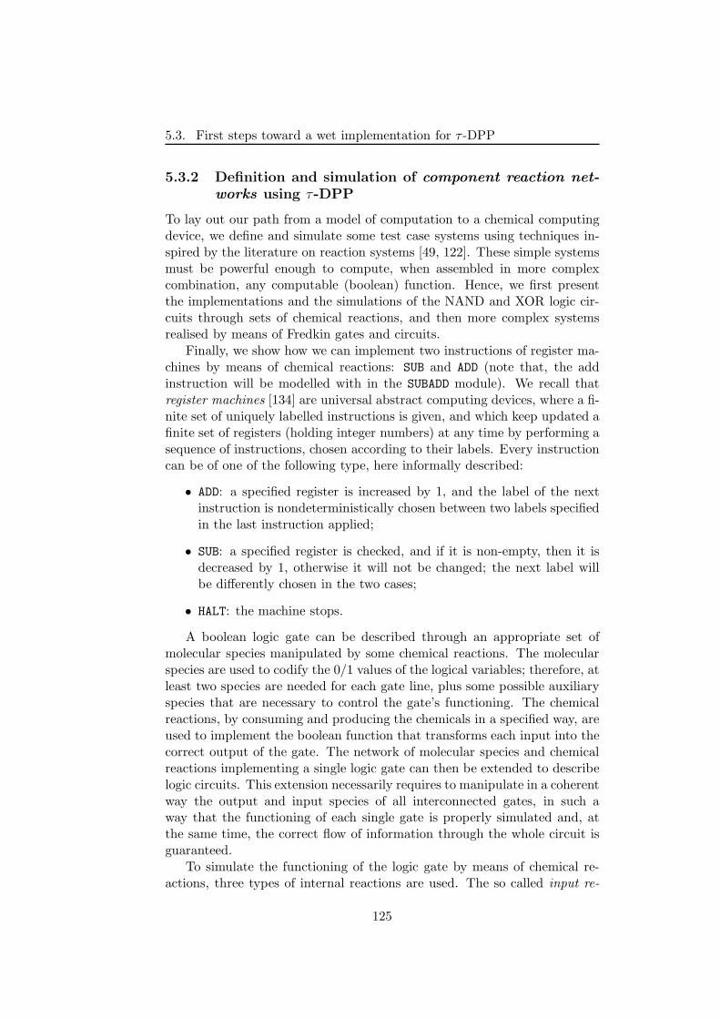
5.3. First steps toward a wet implementation for τ -DPP
5.3.2 Definition and simulation of component reaction net-
works using τ-DPP
To lay out our path from a model of computation to a chemical computingdevice, we define and simulate some test case systems using techniques in-spired by the literature on reaction systems [49, 122]. These simple systemsmust be powerful enough to compute, when assembled in more complexcombination, any computable (boolean) function. Hence, we first presentthe implementations and the simulations of the NAND and XOR logic cir-cuits through sets of chemical reactions, and then more complex systemsrealised by means of Fredkin gates and circuits.
Finally, we show how we can implement two instructions of register ma-chines by means of chemical reactions: SUB and ADD (note that, the addinstruction will be modelled with in the SUBADD module). We recall thatregister machines [134] are universal abstract computing devices, where a fi-nite set of uniquely labelled instructions is given, and which keep updated afinite set of registers (holding integer numbers) at any time by performing asequence of instructions, chosen according to their labels. Every instructioncan be of one of the following type, here informally described:
• ADD: a specified register is increased by 1, and the label of the nextinstruction is nondeterministically chosen between two labels specifiedin the last instruction applied;
• SUB: a specified register is checked, and if it is non-empty, then it isdecreased by 1, otherwise it will not be changed; the next label willbe differently chosen in the two cases;
• HALT: the machine stops.
A boolean logic gate can be described through an appropriate set ofmolecular species manipulated by some chemical reactions. The molecularspecies are used to codify the 0/1 values of the logical variables; therefore, atleast two species are needed for each gate line, plus some possible auxiliaryspecies that are necessary to control the gate’s functioning. The chemicalreactions, by consuming and producing the chemicals in a specified way, areused to implement the boolean function that transforms each input into thecorrect output of the gate. The network of molecular species and chemicalreactions implementing a single logic gate can then be extended to describelogic circuits. This extension necessarily requires to manipulate in a coherentway the output and input species of all interconnected gates, in such away that the functioning of each single gate is properly simulated and, atthe same time, the correct flow of information through the whole circuit isguaranteed.
To simulate the functioning of the logic gate by means of chemical re-actions, three types of internal reactions are used. The so called input re-
125
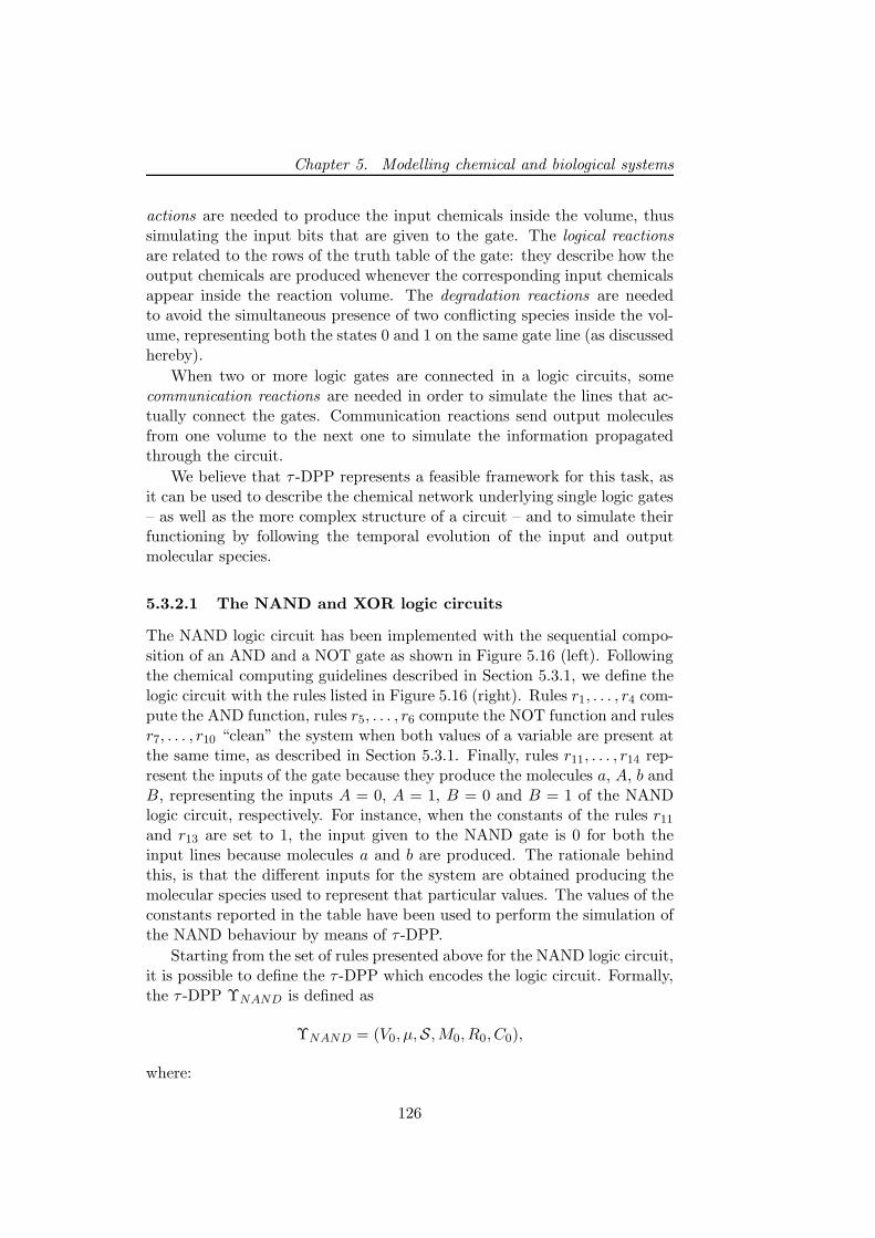
Chapter 5. Modelling chemical and biological systems
actions are needed to produce the input chemicals inside the volume, thussimulating the input bits that are given to the gate. The logical reactionsare related to the rows of the truth table of the gate: they describe how theoutput chemicals are produced whenever the corresponding input chemicalsappear inside the reaction volume. The degradation reactions are neededto avoid the simultaneous presence of two conflicting species inside the vol-ume, representing both the states 0 and 1 on the same gate line (as discussedhereby).
When two or more logic gates are connected in a logic circuits, somecommunication reactions are needed in order to simulate the lines that ac-tually connect the gates. Communication reactions send output moleculesfrom one volume to the next one to simulate the information propagatedthrough the circuit.
We believe that τ -DPP represents a feasible framework for this task, asit can be used to describe the chemical network underlying single logic gates– as well as the more complex structure of a circuit – and to simulate theirfunctioning by following the temporal evolution of the input and outputmolecular species.
5.3.2.1 The NAND and XOR logic circuits
The NAND logic circuit has been implemented with the sequential compo-sition of an AND and a NOT gate as shown in Figure 5.16 (left). Followingthe chemical computing guidelines described in Section 5.3.1, we define thelogic circuit with the rules listed in Figure 5.16 (right). Rules r1, . . . , r4 com-pute the AND function, rules r5, . . . , r6 compute the NOT function and rulesr7, . . . , r10 “clean” the system when both values of a variable are present atthe same time, as described in Section 5.3.1. Finally, rules r11, . . . , r14 rep-resent the inputs of the gate because they produce the molecules a, A, b andB, representing the inputs A = 0, A = 1, B = 0 and B = 1 of the NANDlogic circuit, respectively. For instance, when the constants of the rules r11
and r13 are set to 1, the input given to the NAND gate is 0 for both theinput lines because molecules a and b are produced. The rationale behindthis, is that the different inputs for the system are obtained producing themolecular species used to represent that particular values. The values of theconstants reported in the table have been used to perform the simulation ofthe NAND behaviour by means of τ -DPP.
Starting from the set of rules presented above for the NAND logic circuit,it is possible to define the τ -DPP which encodes the logic circuit. Formally,the τ -DPP ΥNAND is defined as
ΥNAND = (V0, µ,S,M0, R0, C0),
where:
126
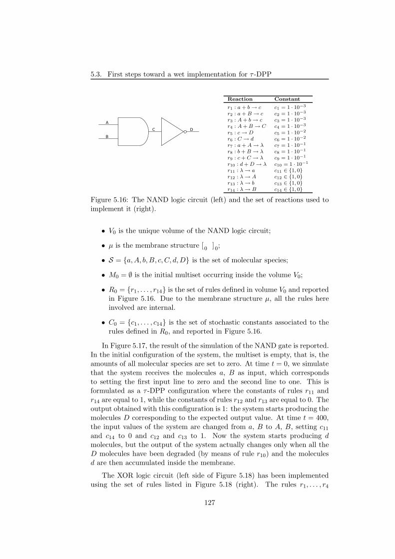
5.3. First steps toward a wet implementation for τ -DPP
Reaction Constant
r1 : a + b → c c1 = 1 · 10−3
r2 : a + B → c c2 = 1 · 10−3
r3 : A + b → c c3 = 1 · 10−3
r4 : A + B → C c4 = 1 · 10−3
r5 : c → D c5 = 1 · 10−2
r6 : C → d c6 = 1 · 10−2
r7 : a + A → λ c7 = 1 · 10−1
r8 : b + B → λ c8 = 1 · 10−1
r9 : c + C → λ c9 = 1 · 10−1
r10 : d + D → λ c10 = 1 · 10−1
r11 : λ → a c11 ∈ 1, 0r12 : λ → A c12 ∈ 1, 0r13 : λ → b c13 ∈ 1, 0r14 : λ → B c14 ∈ 1, 0
Figure 5.16: The NAND logic circuit (left) and the set of reactions used toimplement it (right).
• V0 is the unique volume of the NAND logic circuit;
• µ is the membrane structure [0 ]0;
• S = a,A, b,B, c, C, d,D is the set of molecular species;
• M0 = ∅ is the initial multiset occurring inside the volume V0;
• R0 = r1, . . . , r14 is the set of rules defined in volume V0 and reportedin Figure 5.16. Due to the membrane structure µ, all the rules hereinvolved are internal.
• C0 = c1, . . . , c14 is the set of stochastic constants associated to therules defined in R0, and reported in Figure 5.16.
In Figure 5.17, the result of the simulation of the NAND gate is reported.In the initial configuration of the system, the multiset is empty, that is, theamounts of all molecular species are set to zero. At time t = 0, we simulatethat the system receives the molecules a, B as input, which correspondsto setting the first input line to zero and the second line to one. This isformulated as a τ -DPP configuration where the constants of rules r11 andr14 are equal to 1, while the constants of rules r12 and r13 are equal to 0. Theoutput obtained with this configuration is 1: the system starts producing themolecules D corresponding to the expected output value. At time t = 400,the input values of the system are changed from a, B to A, B, setting c11
and c14 to 0 and c12 and c13 to 1. Now the system starts producing dmolecules, but the output of the system actually changes only when all theD molecules have been degraded (by means of rule r10) and the moleculesd are then accumulated inside the membrane.
The XOR logic circuit (left side of Figure 5.18) has been implementedusing the set of rules listed in Figure 5.18 (right). The rules r1, . . . , r4
127
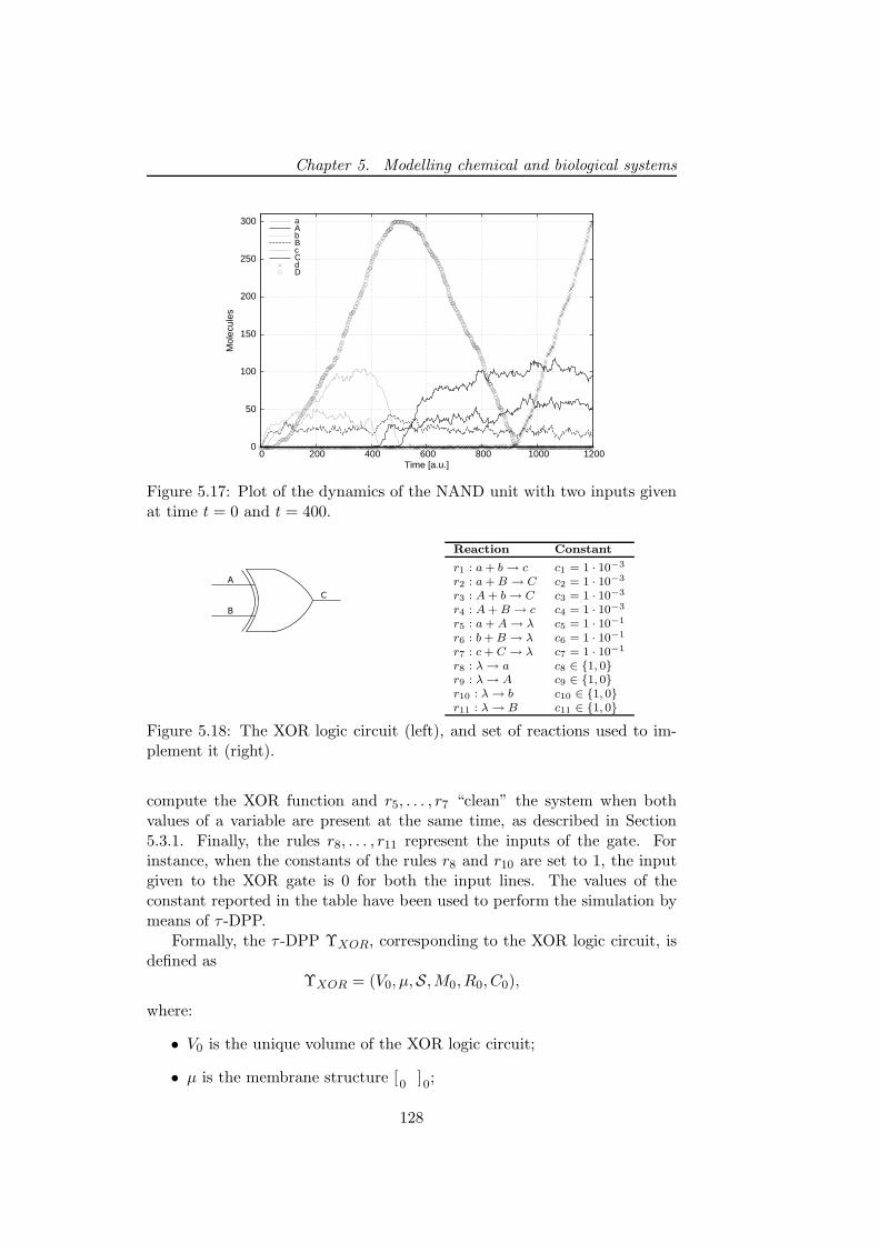
Chapter 5. Modelling chemical and biological systems
0
50
100
150
200
250
300
0 200 400 600 800 1000 1200
Mol
ecul
es
Time [a.u.]
aAbBcCdD
Figure 5.17: Plot of the dynamics of the NAND unit with two inputs givenat time t = 0 and t = 400.
Reaction Constant
r1 : a + b → c c1 = 1 · 10−3
r2 : a + B → C c2 = 1 · 10−3
r3 : A + b → C c3 = 1 · 10−3
r4 : A + B → c c4 = 1 · 10−3
r5 : a + A → λ c5 = 1 · 10−1
r6 : b + B → λ c6 = 1 · 10−1
r7 : c + C → λ c7 = 1 · 10−1
r8 : λ → a c8 ∈ 1, 0r9 : λ → A c9 ∈ 1, 0r10 : λ → b c10 ∈ 1, 0r11 : λ → B c11 ∈ 1, 0
Figure 5.18: The XOR logic circuit (left), and set of reactions used to im-plement it (right).
compute the XOR function and r5, . . . , r7 “clean” the system when bothvalues of a variable are present at the same time, as described in Section5.3.1. Finally, the rules r8, . . . , r11 represent the inputs of the gate. Forinstance, when the constants of the rules r8 and r10 are set to 1, the inputgiven to the XOR gate is 0 for both the input lines. The values of theconstant reported in the table have been used to perform the simulation bymeans of τ -DPP.
Formally, the τ -DPP ΥXOR, corresponding to the XOR logic circuit, isdefined as
ΥXOR = (V0, µ,S,M0, R0, C0),
where:
• V0 is the unique volume of the XOR logic circuit;
• µ is the membrane structure [0 ]0;
128
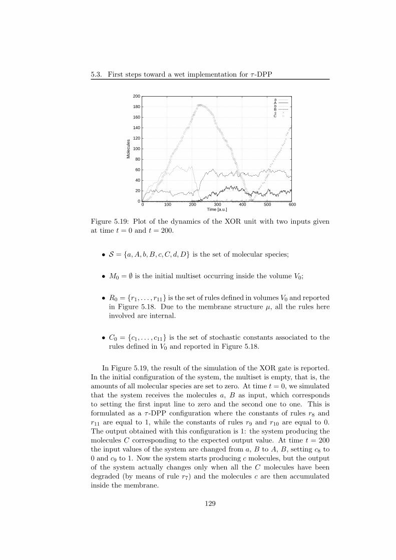
5.3. First steps toward a wet implementation for τ -DPP
0
20
40
60
80
100
120
140
160
180
200
0 100 200 300 400 500 600
Mol
ecul
es
Time [a.u.]
aAbBcC
Figure 5.19: Plot of the dynamics of the XOR unit with two inputs givenat time t = 0 and t = 200.
• S = a,A, b,B, c, C, d,D is the set of molecular species;
• M0 = ∅ is the initial multiset occurring inside the volume V0;
• R0 = r1, . . . , r11 is the set of rules defined in volumes V0 and reportedin Figure 5.18. Due to the membrane structure µ, all the rules hereinvolved are internal.
• C0 = c1, . . . , c11 is the set of stochastic constants associated to therules defined in V0 and reported in Figure 5.18.
In Figure 5.19, the result of the simulation of the XOR gate is reported.In the initial configuration of the system, the multiset is empty, that is, theamounts of all molecular species are set to zero. At time t = 0, we simulatedthat the system receives the molecules a, B as input, which correspondsto setting the first input line to zero and the second one to one. This isformulated as a τ -DPP configuration where the constants of rules r8 andr11 are equal to 1, while the constants of rules r9 and r10 are equal to 0.The output obtained with this configuration is 1: the system producing themolecules C corresponding to the expected output value. At time t = 200the input values of the system are changed from a, B to A, B, setting c8 to0 and c9 to 1. Now the system starts producing c molecules, but the outputof the system actually changes only when all the C molecules have beendegraded (by means of rule r7) and the molecules c are then accumulatedinside the membrane.
129
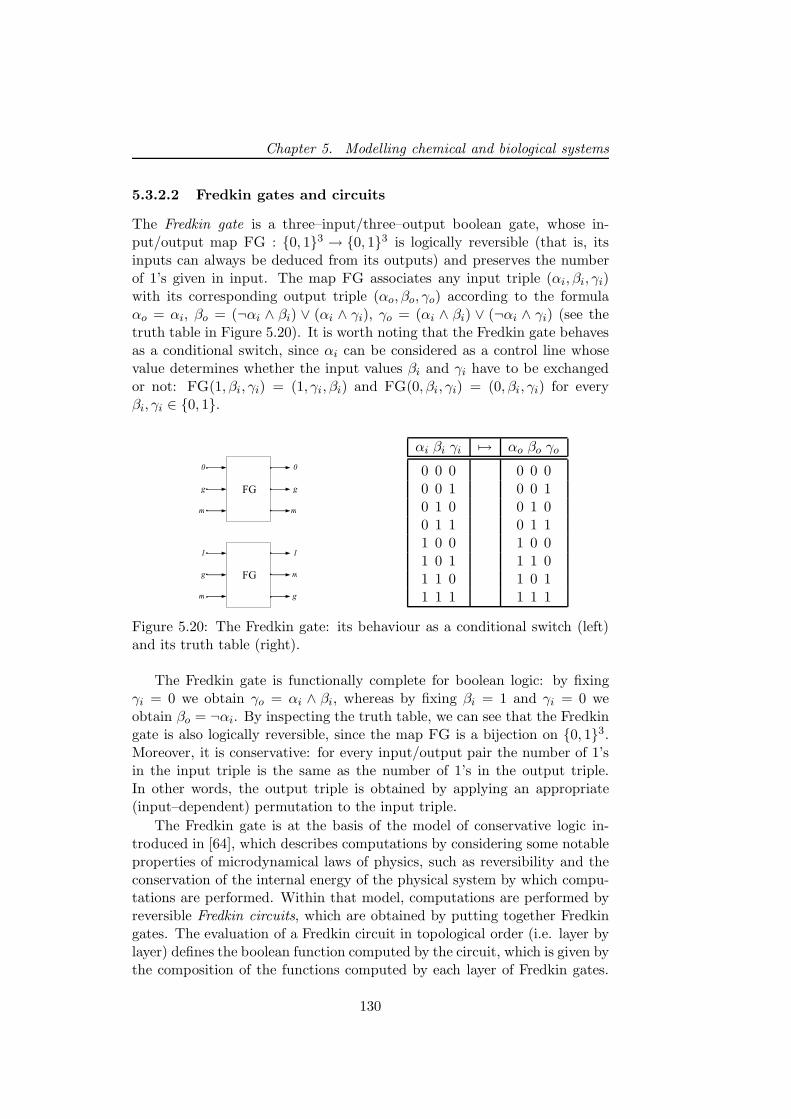
Chapter 5. Modelling chemical and biological systems
5.3.2.2 Fredkin gates and circuits
The Fredkin gate is a three–input/three–output boolean gate, whose in-put/output map FG : 0, 13 → 0, 13 is logically reversible (that is, itsinputs can always be deduced from its outputs) and preserves the numberof 1’s given in input. The map FG associates any input triple (αi, βi, γi)with its corresponding output triple (αo, βo, γo) according to the formulaαo = αi, βo = (¬αi ∧ βi) ∨ (αi ∧ γi), γo = (αi ∧ βi) ∨ (¬αi ∧ γi) (see thetruth table in Figure 5.20). It is worth noting that the Fredkin gate behavesas a conditional switch, since αi can be considered as a control line whosevalue determines whether the input values βi and γi have to be exchangedor not: FG(1, βi, γi) = (1, γi, βi) and FG(0, βi, γi) = (0, βi, γi) for everyβi, γi ∈ 0, 1.
αi βi γi 7→ αo βo γo
0 0 0 0 0 00 0 1 0 0 10 1 0 0 1 00 1 1 0 1 11 0 0 1 0 01 0 1 1 1 01 1 0 1 0 11 1 1 1 1 1
Figure 5.20: The Fredkin gate: its behaviour as a conditional switch (left)and its truth table (right).
The Fredkin gate is functionally complete for boolean logic: by fixingγi = 0 we obtain γo = αi ∧ βi, whereas by fixing βi = 1 and γi = 0 weobtain βo = ¬αi. By inspecting the truth table, we can see that the Fredkingate is also logically reversible, since the map FG is a bijection on 0, 13.Moreover, it is conservative: for every input/output pair the number of 1’sin the input triple is the same as the number of 1’s in the output triple.In other words, the output triple is obtained by applying an appropriate(input–dependent) permutation to the input triple.
The Fredkin gate is at the basis of the model of conservative logic in-troduced in [64], which describes computations by considering some notableproperties of microdynamical laws of physics, such as reversibility and theconservation of the internal energy of the physical system by which compu-tations are performed. Within that model, computations are performed byreversible Fredkin circuits, which are obtained by putting together Fredkingates. The evaluation of a Fredkin circuit in topological order (i.e. layer bylayer) defines the boolean function computed by the circuit, which is given bythe composition of the functions computed by each layer of Fredkin gates.
130
5.3. First steps toward a wet implementation for τ -DPP
The conservativeness of the circuit (preservation of the number of 1’s) isequivalent to the requirement that the output n-tuple is obtained by ap-plying an appropriate (input–dependent) permutation to the correspondinginput n-tuple.
Simulations results In this section, we first show how we can simulate aFredkin gate by means of chemical reactions; then, we present an exampleof a Fredkin circuit, consisting of three gates arranged into two layers, anddescribe how it can be implemented by means of a tissue-like membranestructure.
Concerning the Fredkin gate, we define two different types of molecularspecies for each of its lines; as previously stated, we will denote by meansof lowercase letters the chemicals representing the value 0, while uppercaseletters will be used for the chemicals representing the value 1. In particular,in the following we use: the symbols a,A for both the input αi and outputαo on the first line of the gate; b,B for the input βi and d,D for the outputβo on the second line; c, C for the input γi and e,E for the output γo onthe third line. The rationale behind this choice is that, for the first line –where the output bit is always equal to the input bit – two different chemicalspecies suffice, while for the second and the third lines of the gate – wherethe logic switch is implemented – we will need to distinguish among the 0and 1 bits given as input or generated as output. All these chemicals willbe manipulated inside a single volume of a τ -DPP.
To simulate the functioning of the logic gate by means of chemical re-actions, we use input, logical and degradation reactions (no communicationrule is needed here).
According to the definition of τ -DPP [30], for each chemical reactionthere exists a corresponding stochastic constant that is used to evaluate theprobability of applying that reaction, at each time step, according to thecurrent configuration of the system. In the case of the Fredkin gate, wehave the additional peculiarity that the constants associated to the inputreactions can be modified – actually, turned on and off – at chosen timeinstants during the system evolution (while the constants of logical anddegradation reactions have a value that is fixed during the system evolution,as usual in τ -DPP). So doing, we can simulate the possibility that the inputlines αi, βi, γi of the Fredkin gate can receive a different bit at any chosentime instant. The process can then be repeated at successive time instants,thus allowing the gate to receive any sequence of input bits. Nevertheless,constraints for the activation of input reactions are to be given, in orderto avoid the presence of conflicting input species inside the volume, whichwould correspond to have the two opposite bits on the same input linesimultaneously. The constraints are the following: if an input reaction ri=0
for bit 0 is turned on for one of the three lines of the gate (that is, if species x
131
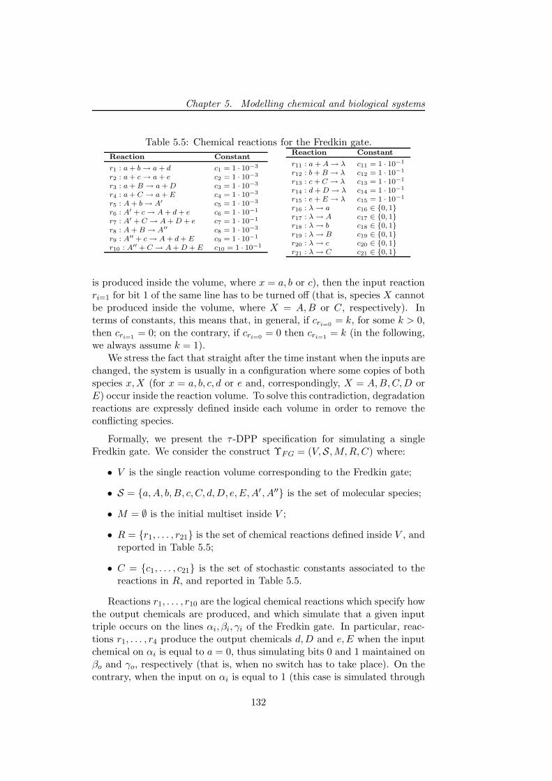
Chapter 5. Modelling chemical and biological systems
Table 5.5: Chemical reactions for the Fredkin gate.
Reaction Constant
r1 : a + b → a + d c1 = 1 · 10−3
r2 : a + c → a + e c2 = 1 · 10−3
r3 : a + B → a + D c3 = 1 · 10−3
r4 : a + C → a + E c4 = 1 · 10−3
r5 : A + b → A′ c5 = 1 · 10−3
r6 : A′ + c → A + d + e c6 = 1 · 10−1
r7 : A′ + C → A + D + e c7 = 1 · 10−1
r8 : A + B → A′′ c8 = 1 · 10−3
r9 : A′′ + c → A + d + E c9 = 1 · 10−1
r10 : A′′ + C → A + D + E c10 = 1 · 10−1
Reaction Constant
r11 : a + A → λ c11 = 1 · 10−1
r12 : b + B → λ c12 = 1 · 10−1
r13 : c + C → λ c13 = 1 · 10−1
r14 : d + D → λ c14 = 1 · 10−1
r15 : e + E → λ c15 = 1 · 10−1
r16 : λ → a c16 ∈ 0, 1r17 : λ → A c17 ∈ 0, 1r18 : λ → b c18 ∈ 0, 1r19 : λ → B c19 ∈ 0, 1r20 : λ → c c20 ∈ 0, 1r21 : λ → C c21 ∈ 0, 1
is produced inside the volume, where x = a, b or c), then the input reactionri=1 for bit 1 of the same line has to be turned off (that is, species X cannotbe produced inside the volume, where X = A,B or C, respectively). Interms of constants, this means that, in general, if cri=0
= k, for some k > 0,then cri=1
= 0; on the contrary, if cri=0= 0 then cri=1
= k (in the following,we always assume k = 1).
We stress the fact that straight after the time instant when the inputs arechanged, the system is usually in a configuration where some copies of bothspecies x,X (for x = a, b, c, d or e and, correspondingly, X = A,B,C,D orE) occur inside the reaction volume. To solve this contradiction, degradationreactions are expressly defined inside each volume in order to remove theconflicting species.
Formally, we present the τ -DPP specification for simulating a singleFredkin gate. We consider the construct ΥFG = (V,S,M,R,C) where:
• V is the single reaction volume corresponding to the Fredkin gate;
• S = a,A, b,B, c, C, d,D, e,E,A′ , A′′ is the set of molecular species;
• M = ∅ is the initial multiset inside V ;
• R = r1, . . . , r21 is the set of chemical reactions defined inside V , andreported in Table 5.5;
• C = c1, . . . , c21 is the set of stochastic constants associated to thereactions in R, and reported in Table 5.5.
Reactions r1, . . . , r10 are the logical chemical reactions which specify howthe output chemicals are produced, and which simulate that a given inputtriple occurs on the lines αi, βi, γi of the Fredkin gate. In particular, reac-tions r1, . . . , r4 produce the output chemicals d,D and e,E when the inputchemical on αi is equal to a = 0, thus simulating bits 0 and 1 maintained onβo and γo, respectively (that is, when no switch has to take place). On thecontrary, when the input on αi is equal to 1 (this case is simulated through
132
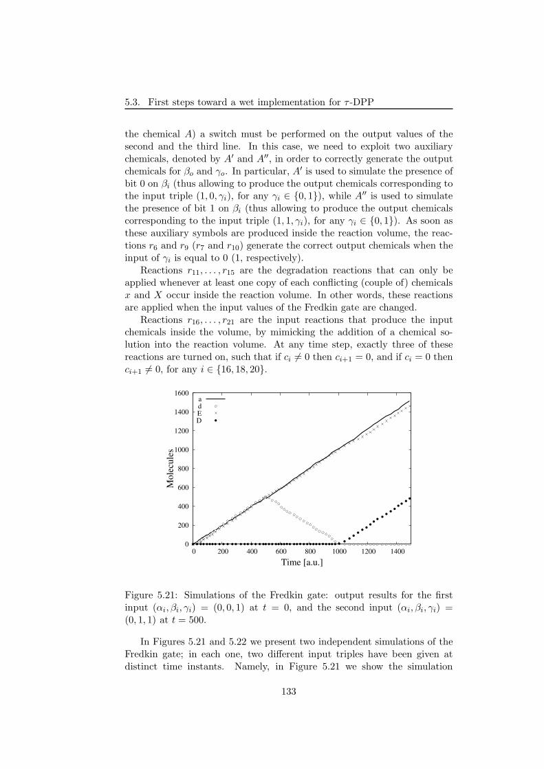
5.3. First steps toward a wet implementation for τ -DPP
the chemical A) a switch must be performed on the output values of thesecond and the third line. In this case, we need to exploit two auxiliarychemicals, denoted by A′ and A′′, in order to correctly generate the outputchemicals for βo and γo. In particular, A′ is used to simulate the presence ofbit 0 on βi (thus allowing to produce the output chemicals corresponding tothe input triple (1, 0, γi), for any γi ∈ 0, 1), while A′′ is used to simulatethe presence of bit 1 on βi (thus allowing to produce the output chemicalscorresponding to the input triple (1, 1, γi), for any γi ∈ 0, 1). As soon asthese auxiliary symbols are produced inside the reaction volume, the reac-tions r6 and r9 (r7 and r10) generate the correct output chemicals when theinput of γi is equal to 0 (1, respectively).
Reactions r11, . . . , r15 are the degradation reactions that can only beapplied whenever at least one copy of each conflicting (couple of) chemicalsx and X occur inside the reaction volume. In other words, these reactionsare applied when the input values of the Fredkin gate are changed.
Reactions r16, . . . , r21 are the input reactions that produce the inputchemicals inside the volume, by mimicking the addition of a chemical so-lution into the reaction volume. At any time step, exactly three of thesereactions are turned on, such that if ci 6= 0 then ci+1 = 0, and if ci = 0 thenci+1 6= 0, for any i ∈ 16, 18, 20.
0
200
400
600
800
1000
1200
1400
1600
0 200 400 600 800 1000 1200 1400
Mole
cule
s
Time [a.u.]
adED
Figure 5.21: Simulations of the Fredkin gate: output results for the firstinput (αi, βi, γi) = (0, 0, 1) at t = 0, and the second input (αi, βi, γi) =(0, 1, 1) at t = 500.
In Figures 5.21 and 5.22 we present two independent simulations of theFredkin gate; in each one, two different input triples have been given atdistinct time instants. Namely, in Figure 5.21 we show the simulation
133
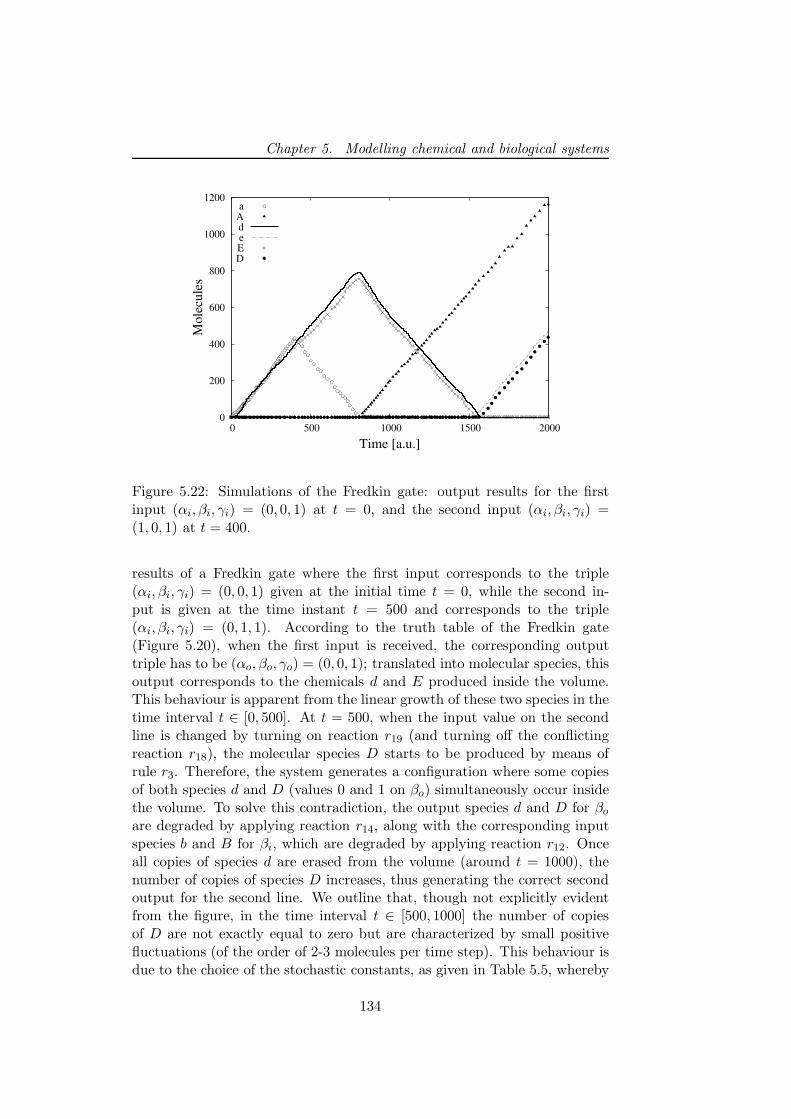
Chapter 5. Modelling chemical and biological systems
0
200
400
600
800
1000
1200
0 500 1000 1500 2000
Mole
cule
s
Time [a.u.]
aAdeED
Figure 5.22: Simulations of the Fredkin gate: output results for the firstinput (αi, βi, γi) = (0, 0, 1) at t = 0, and the second input (αi, βi, γi) =(1, 0, 1) at t = 400.
results of a Fredkin gate where the first input corresponds to the triple(αi, βi, γi) = (0, 0, 1) given at the initial time t = 0, while the second in-put is given at the time instant t = 500 and corresponds to the triple(αi, βi, γi) = (0, 1, 1). According to the truth table of the Fredkin gate(Figure 5.20), when the first input is received, the corresponding outputtriple has to be (αo, βo, γo) = (0, 0, 1); translated into molecular species, thisoutput corresponds to the chemicals d and E produced inside the volume.This behaviour is apparent from the linear growth of these two species in thetime interval t ∈ [0, 500]. At t = 500, when the input value on the secondline is changed by turning on reaction r19 (and turning off the conflictingreaction r18), the molecular species D starts to be produced by means ofrule r3. Therefore, the system generates a configuration where some copiesof both species d and D (values 0 and 1 on βo) simultaneously occur insidethe volume. To solve this contradiction, the output species d and D for βo
are degraded by applying reaction r14, along with the corresponding inputspecies b and B for βi, which are degraded by applying reaction r12. Onceall copies of species d are erased from the volume (around t = 1000), thenumber of copies of species D increases, thus generating the correct secondoutput for the second line. We outline that, though not explicitly evidentfrom the figure, in the time interval t ∈ [500, 1000] the number of copiesof D are not exactly equal to zero but are characterized by small positivefluctuations (of the order of 2-3 molecules per time step). This behaviour isdue to the choice of the stochastic constants, as given in Table 5.5, whereby
134
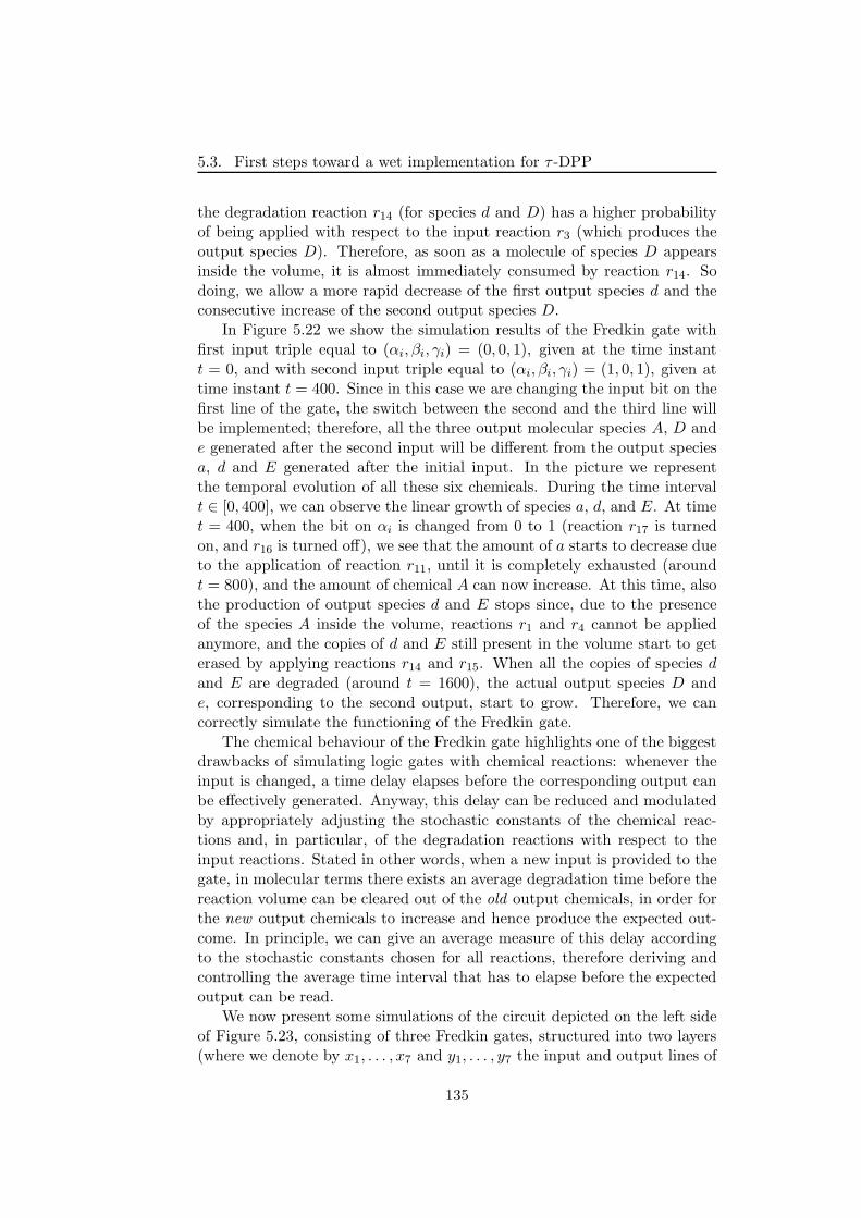
5.3. First steps toward a wet implementation for τ -DPP
the degradation reaction r14 (for species d and D) has a higher probabilityof being applied with respect to the input reaction r3 (which produces theoutput species D). Therefore, as soon as a molecule of species D appearsinside the volume, it is almost immediately consumed by reaction r14. Sodoing, we allow a more rapid decrease of the first output species d and theconsecutive increase of the second output species D.
In Figure 5.22 we show the simulation results of the Fredkin gate withfirst input triple equal to (αi, βi, γi) = (0, 0, 1), given at the time instantt = 0, and with second input triple equal to (αi, βi, γi) = (1, 0, 1), given attime instant t = 400. Since in this case we are changing the input bit on thefirst line of the gate, the switch between the second and the third line willbe implemented; therefore, all the three output molecular species A, D ande generated after the second input will be different from the output speciesa, d and E generated after the initial input. In the picture we representthe temporal evolution of all these six chemicals. During the time intervalt ∈ [0, 400], we can observe the linear growth of species a, d, and E. At timet = 400, when the bit on αi is changed from 0 to 1 (reaction r17 is turnedon, and r16 is turned off), we see that the amount of a starts to decrease dueto the application of reaction r11, until it is completely exhausted (aroundt = 800), and the amount of chemical A can now increase. At this time, alsothe production of output species d and E stops since, due to the presenceof the species A inside the volume, reactions r1 and r4 cannot be appliedanymore, and the copies of d and E still present in the volume start to geterased by applying reactions r14 and r15. When all the copies of species dand E are degraded (around t = 1600), the actual output species D ande, corresponding to the second output, start to grow. Therefore, we cancorrectly simulate the functioning of the Fredkin gate.
The chemical behaviour of the Fredkin gate highlights one of the biggestdrawbacks of simulating logic gates with chemical reactions: whenever theinput is changed, a time delay elapses before the corresponding output canbe effectively generated. Anyway, this delay can be reduced and modulatedby appropriately adjusting the stochastic constants of the chemical reac-tions and, in particular, of the degradation reactions with respect to theinput reactions. Stated in other words, when a new input is provided to thegate, in molecular terms there exists an average degradation time before thereaction volume can be cleared out of the old output chemicals, in order forthe new output chemicals to increase and hence produce the expected out-come. In principle, we can give an average measure of this delay accordingto the stochastic constants chosen for all reactions, therefore deriving andcontrolling the average time interval that has to elapse before the expectedoutput can be read.
We now present some simulations of the circuit depicted on the left sideof Figure 5.23, consisting of three Fredkin gates, structured into two layers(where we denote by x1, . . . , x7 and y1, . . . , y7 the input and output lines of
135
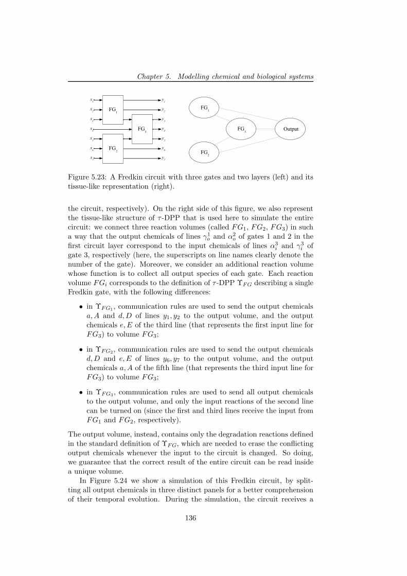
Chapter 5. Modelling chemical and biological systems
Figure 5.23: A Fredkin circuit with three gates and two layers (left) and itstissue-like representation (right).
the circuit, respectively). On the right side of this figure, we also representthe tissue-like structure of τ -DPP that is used here to simulate the entirecircuit: we connect three reaction volumes (called FG1, FG2, FG3) in sucha way that the output chemicals of lines γ1
o and α2o of gates 1 and 2 in the
first circuit layer correspond to the input chemicals of lines α3i and γ3
i ofgate 3, respectively (here, the superscripts on line names clearly denote thenumber of the gate). Moreover, we consider an additional reaction volumewhose function is to collect all output species of each gate. Each reactionvolume FGi corresponds to the definition of τ -DPP ΥFG describing a singleFredkin gate, with the following differences:
• in ΥFG1, communication rules are used to send the output chemicals
a,A and d,D of lines y1, y2 to the output volume, and the outputchemicals e,E of the third line (that represents the first input line forFG3) to volume FG3;
• in ΥFG2, communication rules are used to send the output chemicals
d,D and e,E of lines y6, y7 to the output volume, and the outputchemicals a,A of the fifth line (that represents the third input line forFG3) to volume FG3;
• in ΥFG3, communication rules are used to send all output chemicals
to the output volume, and only the input reactions of the second linecan be turned on (since the first and third lines receive the input fromFG1 and FG2, respectively).
The output volume, instead, contains only the degradation reactions definedin the standard definition of ΥFG, which are needed to erase the conflictingoutput chemicals whenever the input to the circuit is changed. So doing,we guarantee that the correct result of the entire circuit can be read insidea unique volume.
In Figure 5.24 we show a simulation of this Fredkin circuit, by split-ting all output chemicals in three distinct panels for a better comprehensionof their temporal evolution. During the simulation, the circuit receives a
136
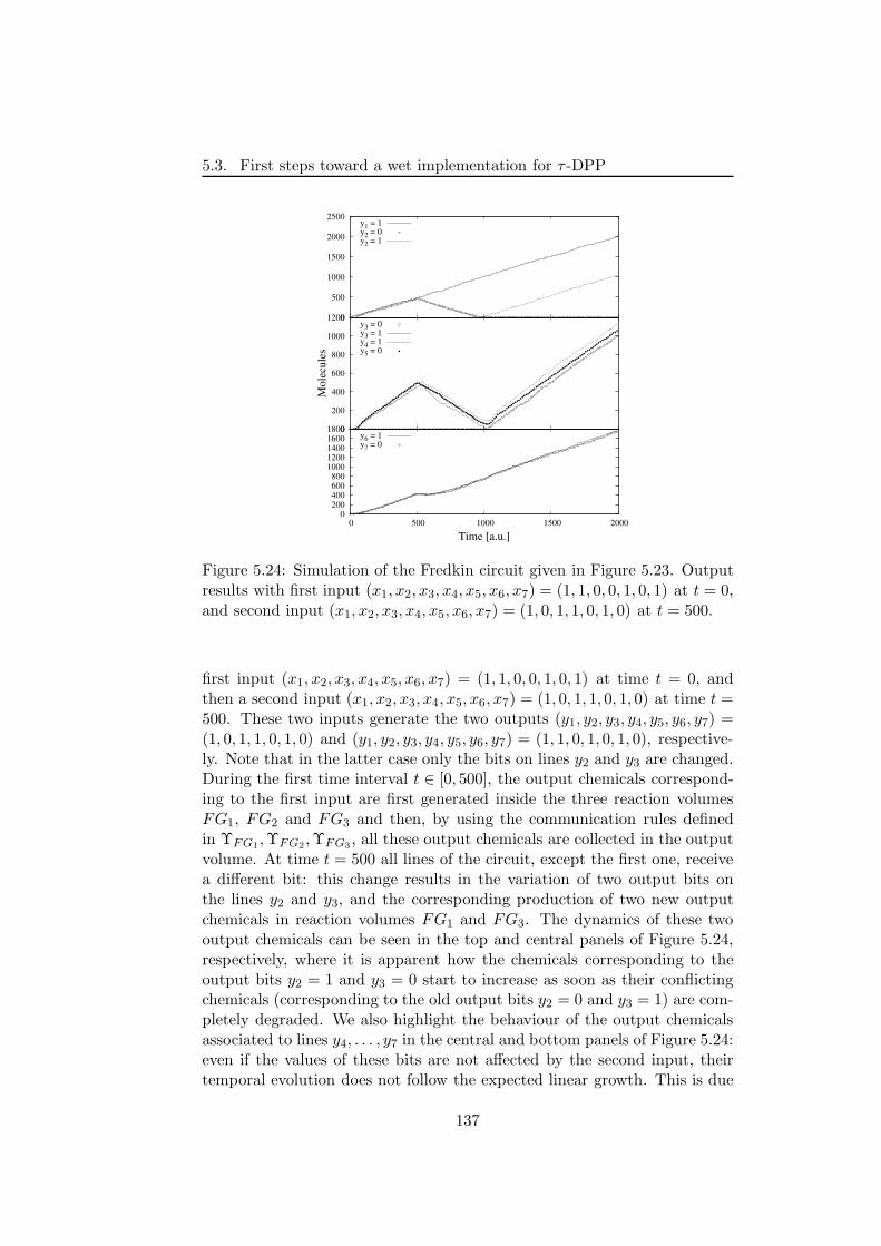
5.3. First steps toward a wet implementation for τ -DPP
0
500
1000
1500
2000
2500y1 = 1y2 = 0y2 = 1
0
200
400
600
800
1000
1200M
ole
cule
sy3 = 0y3 = 1y4 = 1y5 = 0
0 200 400 600 800
1000 1200 1400 1600 1800
0 500 1000 1500 2000
Time [a.u.]
y6 = 1y7 = 0
Figure 5.24: Simulation of the Fredkin circuit given in Figure 5.23. Outputresults with first input (x1, x2, x3, x4, x5, x6, x7) = (1, 1, 0, 0, 1, 0, 1) at t = 0,and second input (x1, x2, x3, x4, x5, x6, x7) = (1, 0, 1, 1, 0, 1, 0) at t = 500.
first input (x1, x2, x3, x4, x5, x6, x7) = (1, 1, 0, 0, 1, 0, 1) at time t = 0, andthen a second input (x1, x2, x3, x4, x5, x6, x7) = (1, 0, 1, 1, 0, 1, 0) at time t =500. These two inputs generate the two outputs (y1, y2, y3, y4, y5, y6, y7) =(1, 0, 1, 1, 0, 1, 0) and (y1, y2, y3, y4, y5, y6, y7) = (1, 1, 0, 1, 0, 1, 0), respective-ly. Note that in the latter case only the bits on lines y2 and y3 are changed.During the first time interval t ∈ [0, 500], the output chemicals correspond-ing to the first input are first generated inside the three reaction volumesFG1, FG2 and FG3 and then, by using the communication rules definedin ΥFG1
,ΥFG2,ΥFG3
, all these output chemicals are collected in the outputvolume. At time t = 500 all lines of the circuit, except the first one, receivea different bit: this change results in the variation of two output bits onthe lines y2 and y3, and the corresponding production of two new outputchemicals in reaction volumes FG1 and FG3. The dynamics of these twooutput chemicals can be seen in the top and central panels of Figure 5.24,respectively, where it is apparent how the chemicals corresponding to theoutput bits y2 = 1 and y3 = 0 start to increase as soon as their conflictingchemicals (corresponding to the old output bits y2 = 0 and y3 = 1) are com-pletely degraded. We also highlight the behaviour of the output chemicalsassociated to lines y4, . . . , y7 in the central and bottom panels of Figure 5.24:even if the values of these bits are not affected by the second input, theirtemporal evolution does not follow the expected linear growth. This is due
137

Chapter 5. Modelling chemical and biological systems
to the fact that, when changing the value of x5 from the first to the secondinput, the degradation delay required to consume all conflicting species isnow impacting on the dynamics of the output lines y6 and y7 in a weak way(they just show a smooth and fast decrease before they can start to growagain, as shown in the bottom panel), and of the output lines y4 and y5 in asharper way (they follow a dynamics similar to that of y3, as shown in thecentral panel).
It is thus clear that, similarly to the single Fredkin gate, when simulatinga change of the input value in a circuit, we have to wait for species degra-dation before the effective new output is generated. This time, however,the topology of the circuit (number of layers and gates, and their inter-connections) brings about an additional “noise” on the temporal evolutionof chemicals. This is due to an imbalance of the quantity of the chemicalspecies corresponding to the lines that are not connected to other gates ina successive layer (e.g. the first and second lines of FG1, and the secondand third lines of FG2 in Figure 5.23), with respect to the quantity of thespecies corresponding to the lines that become input for some other gate ina successive layer (e.g. the third line of FG1 and the first line of FG2 inFigure 5.23). Such imbalance could be avoided by providing a different formof the circuit. In fact, in [105] it is shown how to transform any Fredkin cir-cuit, consisting of a given number of gates arranged in a fixed configurationof layers, into an equivalent (normalized) Fredkin circuit, where each layercontains the same number of gates (to this aim, auxiliary gates and lines areused). By considering this kind of normalized circuits, it is possible to sim-ulate their functioning through chemical reaction systems without havingto deal with the aforementioned problems of degradation delays. However,in this case we would have to handle more complex systems, consisting ofmore volumes and many more chemical species and reactions.
5.3.2.3 The SUB instruction
We now describe and simulate a τ -DPP composed by 2 volumes reproduc-ing the behaviour of a SUB instruction of a register machine. This type ofinstruction is important because it hides a conditional behaviour, checkingwhether a register is zero or not, and can be implemented by choosing adifferent label for the next instruction according to the register value. Theavailability of conditional instructions is a key issue in computing devices.
We implement a system where the quantity stored inside the register isrepresented by the amount of molecules u occurring in volume V1. The labelfor the next instruction is related to the production of molecules p or z involume V0. Finally, to start the system, molecules s are produced inside V0.s′ and z′ are additional molecular species used to implement the instruction.
In order to correctly execute the SUB instruction, when molecules s aresent inside the volume V1, the system first checks if the register value is
138
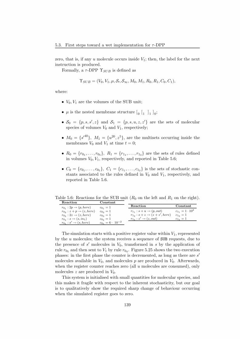
5.3. First steps toward a wet implementation for τ -DPP
zero, that is, if any u molecule occurs inside V1; then, the label for the nextinstruction is produced.
Formally, a τ -DPP ΥSUB is defined as
ΥSUB = (V0, V1, µ,S′,S∞,M0,M1, R0, R1, C0, C1),
where:
• V0, V1 are the volumes of the SUB unit;
• µ is the nested membrane structure [0 [1 ]1 ]0;
• S0 = p, s, s′, z and S1 = p, s, u, z, z′ are the sets of molecularspecies of volumes V0 and V1, respectively;
• M0 = s′40, M1 = u20, z5, are the multisets occurring inside themembranes V0 and V1 at time t = 0;
• R0 = r01, . . . , r05
, R1 = r11, . . . , r13
are the sets of rules definedin volumes V0, V1, respectively, and reported in Table 5.6;
• C0 = c01, . . . , c05
, C1 = c11, . . . , c13
is the sets of stochastic con-stants associated to the rules defined in V0 and V1, respectively, andreported in Table 5.6.
Table 5.6: Reactions for the SUB unit (R0 on the left and R1 on the right).Reaction Constant
r01: 2p → (p, here) c01
= 1r02
: z + p → (z, here) c02= 1
r03: 2z → (z, here) c03
= 1r04
: s → (s, in1) c04= 1
r05: s′ → (s, here) c05
= 6 · 10−2
Reaction Constant
r11: s + u → (p, out) c11
= 1 · 103
r12: s + z → (z + z′, here) c12
= 1r13
: z′ → (z, out) c13= 1
The simulation starts with a positive register value within V1, representedby the u molecules; the system receives a sequence of SUB requests, due tothe presence of s′ molecules in V0, transformed in s by the application ofrule r05
and then sent to V1 by rule r04. Figure 5.25 shows the two execution
phases: in the first phase the counter is decremented, as long as there are s′
molecules available in V0, and molecules p are produced in V0. Afterwards,when the register counter reaches zero (all u molecules are consumed), onlymolecules z are produced in V0.
This system is initialised with small quantities for molecular species, andthis makes it fragile with respect to the inherent stochasticity, but our goalis to qualitatively show the required sharp change of behaviour occurringwhen the simulated register goes to zero.
139
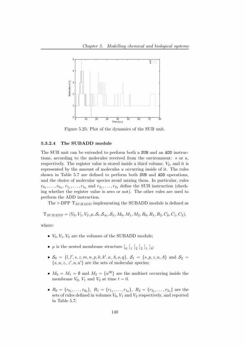
Chapter 5. Modelling chemical and biological systems
0
1
2
3
4
5
0 10 20 30 40 50 60 70 80
Mol
ecul
es in
V0
Time [a.u.]
pz
Figure 5.25: Plot of the dynamics of the SUB unit.
5.3.2.4 The SUBADD module
The SUB unit can be extended to perform both a SUB and an ADD instruc-tions, according to the molecules received from the environment: s or a,respectively. The register value is stored inside a third volume, V2, and it isrepresented by the amount of molecules u occurring inside of it. The rulesshown in Table 5.7 are defined to perform both SUB and ADD operations,and the choice of molecular species avoid mixing them. In particular, rulesr01
, . . . , r04, r11
, . . . , r16and r21
, . . . , r23define the SUB instruction (check-
ing whether the register value is zero or not). The other rules are used toperform the ADD instruction.
The τ -DPP ΥSUBADD implementing the SUBADD module is defined as
ΥSUBADD = (V0, V1, V2, µ,S′,S∞,S∈,M0,M1,M2, R0, R1, R2, C0, C1, C2),
where:
• V0, V1, V2 are the volumes of the SUBADD module;
• µ is the nested membrane structure [0 [1 [2 ]2 ]1 ]0;
• S0 = l, l′, s, z,m, n, p, k, k′, a,A, o, q, S1 = s, p, z, a,A and S2 =s, u, z, z′, a, a′ are the sets of molecular species;
• M0 = M1 = ∅ and M2 = u30 are the multiset occurring inside themembrane V0, V1 and V2 at time t = 0.
• R0 = r01, . . . , r08
, R1 = r11, . . . , r18
, R2 = r21, . . . , r25
are thesets of rules defined in volumes V0, V1 and V2 respectively, and reportedin Table 5.7;
140
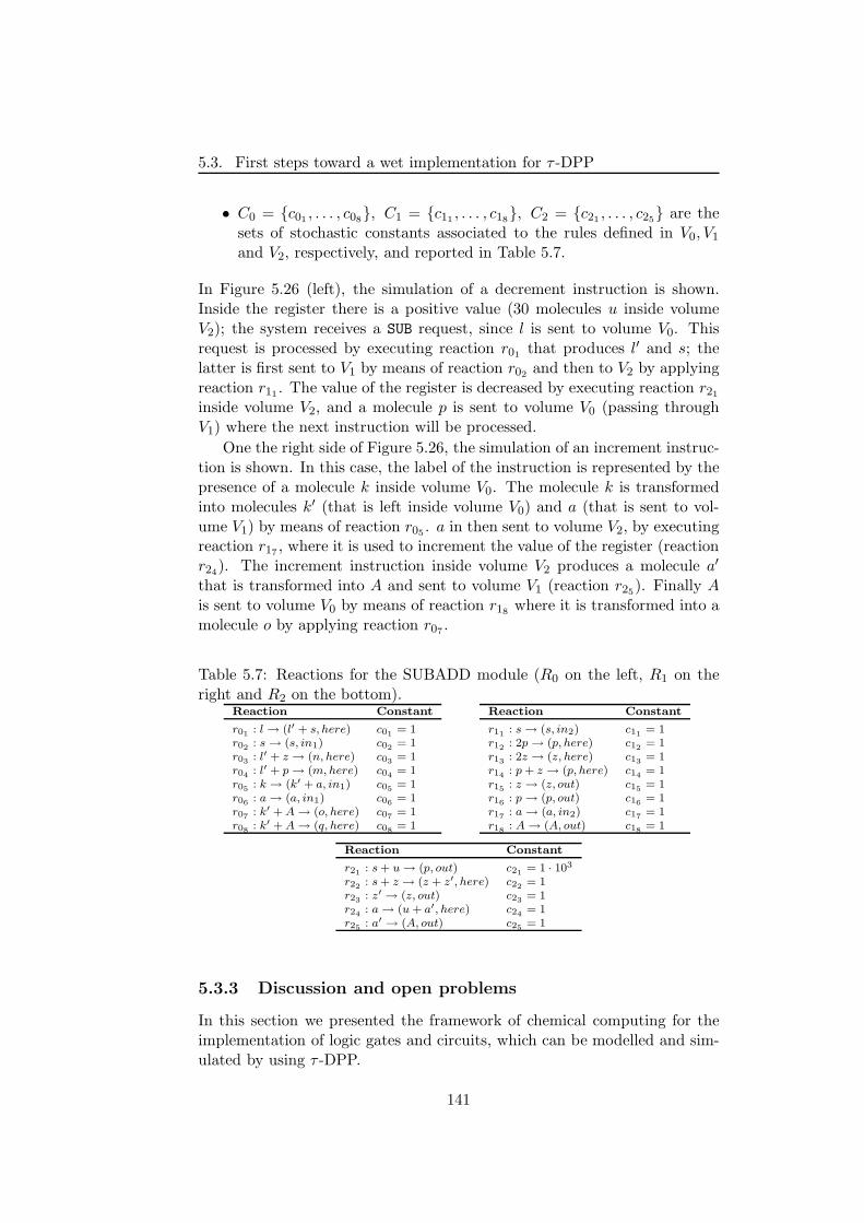
5.3. First steps toward a wet implementation for τ -DPP
• C0 = c01, . . . , c08
, C1 = c11, . . . , c18
, C2 = c21, . . . , c25
are thesets of stochastic constants associated to the rules defined in V0, V1
and V2, respectively, and reported in Table 5.7.
In Figure 5.26 (left), the simulation of a decrement instruction is shown.Inside the register there is a positive value (30 molecules u inside volumeV2); the system receives a SUB request, since l is sent to volume V0. Thisrequest is processed by executing reaction r01
that produces l′ and s; thelatter is first sent to V1 by means of reaction r02
and then to V2 by applyingreaction r11
. The value of the register is decreased by executing reaction r21
inside volume V2, and a molecule p is sent to volume V0 (passing throughV1) where the next instruction will be processed.
One the right side of Figure 5.26, the simulation of an increment instruc-tion is shown. In this case, the label of the instruction is represented by thepresence of a molecule k inside volume V0. The molecule k is transformedinto molecules k′ (that is left inside volume V0) and a (that is sent to vol-ume V1) by means of reaction r05
. a in then sent to volume V2, by executingreaction r17
, where it is used to increment the value of the register (reactionr24
). The increment instruction inside volume V2 produces a molecule a′
that is transformed into A and sent to volume V1 (reaction r25). Finally A
is sent to volume V0 by means of reaction r18where it is transformed into a
molecule o by applying reaction r07.
Table 5.7: Reactions for the SUBADD module (R0 on the left, R1 on theright and R2 on the bottom).
Reaction Constant
r01: l → (l′ + s, here) c01
= 1r02
: s → (s, in1) c02= 1
r03: l′ + z → (n, here) c03
= 1r04
: l′ + p → (m, here) c04= 1
r05: k → (k′ + a, in1) c05
= 1r06
: a → (a, in1) c06= 1
r07: k′ + A → (o, here) c07
= 1r08
: k′ + A → (q, here) c08= 1
Reaction Constant
r11: s → (s, in2) c11
= 1r12
: 2p → (p, here) c12= 1
r13: 2z → (z, here) c13
= 1r14
: p + z → (p, here) c14= 1
r15: z → (z, out) c15
= 1r16
: p → (p, out) c16= 1
r17: a → (a, in2) c17
= 1r18
: A → (A, out) c18= 1
Reaction Constant
r21: s + u → (p, out) c21
= 1 · 103
r22: s + z → (z + z′, here) c22
= 1r23
: z′ → (z, out) c23= 1
r24: a → (u + a′, here) c24
= 1r25
: a′ → (A, out) c25= 1
5.3.3 Discussion and open problems
In this section we presented the framework of chemical computing for theimplementation of logic gates and circuits, which can be modelled and sim-ulated by using τ -DPP.
141
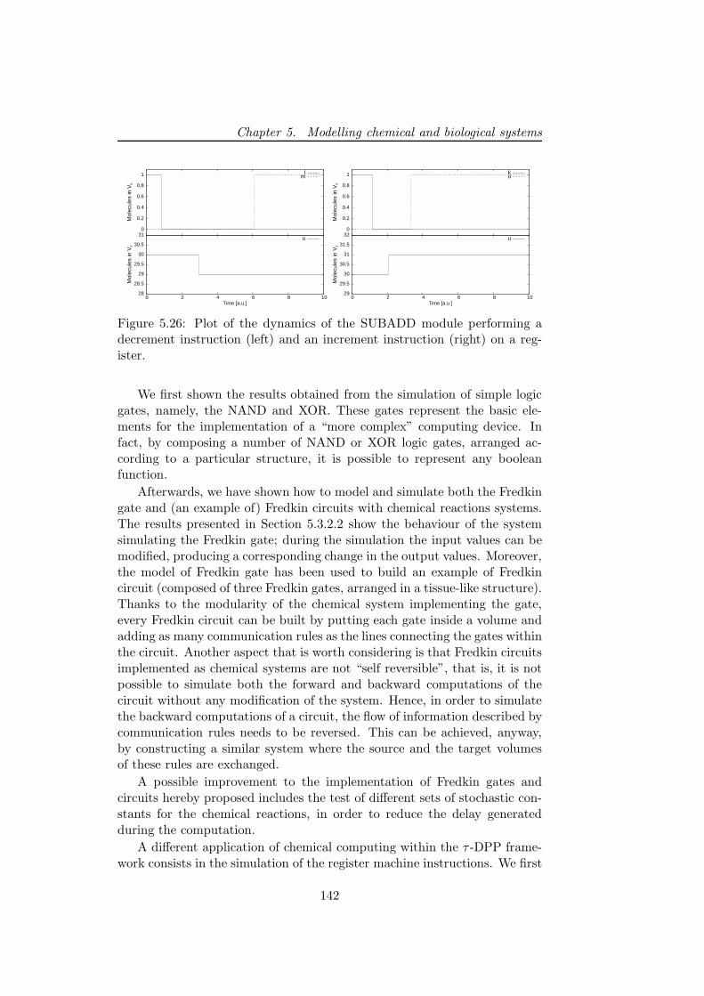
Chapter 5. Modelling chemical and biological systems
0
0.2
0.4
0.6
0.8
1
Mol
ecul
es in
V0
lm
28
28.5
29
29.5
30
30.5
31
0 2 4 6 8 10
Mol
ecul
es in
V2
Time [a.u.]
u
0
0.2
0.4
0.6
0.8
1
Mol
ecul
es in
V0
ko
29
29.5
30
30.5
31
31.5
32
0 2 4 6 8 10
Mol
ecul
es in
V2
Time [a.u.]
u
Figure 5.26: Plot of the dynamics of the SUBADD module performing adecrement instruction (left) and an increment instruction (right) on a reg-ister.
We first shown the results obtained from the simulation of simple logicgates, namely, the NAND and XOR. These gates represent the basic ele-ments for the implementation of a “more complex” computing device. Infact, by composing a number of NAND or XOR logic gates, arranged ac-cording to a particular structure, it is possible to represent any booleanfunction.
Afterwards, we have shown how to model and simulate both the Fredkingate and (an example of) Fredkin circuits with chemical reactions systems.The results presented in Section 5.3.2.2 show the behaviour of the systemsimulating the Fredkin gate; during the simulation the input values can bemodified, producing a corresponding change in the output values. Moreover,the model of Fredkin gate has been used to build an example of Fredkincircuit (composed of three Fredkin gates, arranged in a tissue-like structure).Thanks to the modularity of the chemical system implementing the gate,every Fredkin circuit can be built by putting each gate inside a volume andadding as many communication rules as the lines connecting the gates withinthe circuit. Another aspect that is worth considering is that Fredkin circuitsimplemented as chemical systems are not “self reversible”, that is, it is notpossible to simulate both the forward and backward computations of thecircuit without any modification of the system. Hence, in order to simulatethe backward computations of a circuit, the flow of information described bycommunication rules needs to be reversed. This can be achieved, anyway,by constructing a similar system where the source and the target volumesof these rules are exchanged.
A possible improvement to the implementation of Fredkin gates andcircuits hereby proposed includes the test of different sets of stochastic con-stants for the chemical reactions, in order to reduce the delay generatedduring the computation.
A different application of chemical computing within the τ -DPP frame-work consists in the simulation of the register machine instructions. We first
142
5.3. First steps toward a wet implementation for τ -DPP
modelled the SUB instruction as a system composed by two membranes,which has a conditional behaviour, checking whether a register is zero ornot. We then presented the results obtained by simulating the SUBADDmodule. Note that, by using these modules, we can outline the structureof a τ -DPP system simulating a complete register machine with just threelevels of nested membranes, namely, the skin membrane, enclosing a numberof “register” membranes structured like volume V1 in SUBADD module.
The key idea to be developed, is to simulate the steps of the registermachine by having inside the skin membrane the molecules representing thecurrent instruction label.
For instance, if instruction l increments register r, then the rules wouldbe defined to produce molecules ar and send them to an internal membranerepresenting register r. That internal membrane will then produce moleculesAr, and a rule in the skin membrane would transform pairs of moleculesl+Ar into (non-deterministically chosen) molecules m, where m is one of theoutcome labels specified by the ADD instruction being simulated. Additionaldetails related to the halting of the computation need to be specified.
This approach to the implementation of complex systems leads to someopen problems worth being studied. How does the passage from single simplecomponents to complete universal devices, with the required connectivity,scale? It is well known that small universal register machines can be built,as shown in [102], but their τ -DPP implementation, and eventually theirchemical system implementation have to be evaluated.
Moreover, the computational efficiency of these systems can be studied,for instance with respect to NP-complete problems such as SAT. Anyway,the usual trade-off between space and time in structural complexity perhapshas to be applied with negative results to τ -DPP, since objects could ex-ponentially grow in polynomial time (by using rules like p → 2p), but thespace structure of volumes is fixed. Finally, also the stochasticity of τ -DPPhas to be considered in the computational complexity study.
143
Chapter 5. Modelling chemical and biological systems
5.4 A study on the combined interplay betweenstochastic fluctuations and the number of flag-
ella in bacterial chemotaxis
Chemotaxis is an efficient signal transduction pathway which allows bacterialcells to move directionally, in response to specific attractants or repellentsoccurring in their surroundings. The pathway consists of several trans-membrane and cytoplasmic proteins acting as signal sensors and responseregulators [97], which rule the reversal of the flagellar motor (governed bythe phosphorylation and dephosphorylation of a key protein, CheY). Thisprocess induces a switch between running and tumbling movements, witha frequency that allows a temporal sampling (through random walks) ofhomogeneous environments. Anyway, in the presence of a gradient of at-tractants or repellents, the bacteria are able to respond quickly by reducingthe frequency of flagellar reversal between clockwise and counterclockwiserotations, which cause a longer running motion in a biased direction. Thefrequency of switching is then reset to the random walk level if the concen-tration of the external ligands remains constant in time. At the molecularscale, this adaptation property is implemented by the coordinated action ofmethyltransferase and methylesterase proteins acting on the transmembranereceptors.
The genetic regulation and biochemical functions of the proteins in-volved in chemotaxis are well known, and several models have been proposedto study their complex interplay as well as the robustness of this system[5, 186, 138, 106, 110, 170]. In the model we present hereby, we considervery detailed protein–protein interactions for the chemotactic pathway in E.coli, in response to attractant molecules, which sum up to 62 biochemicalreactions and 32 molecular species. The temporal evolution of the phos-phorylated form of CheY (CheYp) is studied through stochastic simulationsperformed by means of the τ -DPP algorithm presented in Chapter 4. Inparticular, we investigate the CheYp dynamics under different conditions,such as the deletion of other proteins involved in the pathway, the additionof distinct amounts of external ligand, and the effect of different methylationstates.
We then propose an analysis on the interplay between the stochasticfluctuations of CheYp and the number of cellular flagella – around half adozen in E. coli – in the individual bacterium, to the aim of devising themean time periods during which the cell either performs a running or atumbling motion. Experimental observations show that the running motionrequires all flagella to be simultaneously synchronized in the counterclock-wise rotation, which occurs when CheYp is not interacting with the proteinsregulating the flagellar motor; on the contrary, when at least one flagellumis not coordinated with the others, then the bacterium performs a tum-
144
5.4. A study on the combined interplay between stochastic fluctuationsand the number of flagella in bacterial chemotaxis
bling movement. To distinguish between these two states, we assume thatthe cell is sensitive to a threshold level of CheYp, that is evaluated as themean value of CheYp at steady state. Because of stochastic fluctuations,the amount of CheYp will randomly switch from below to above this value,thus reversing the rotation from counterclockwise to clockwise rotations ofeach flagellum. The original contribution presented here, is the link betweensynchronization of flagella and stochastic fluctuations of CheYp, as the corereason that stands at the basis of chemotactic motion. We have defined aprocedure to identify the synchronization of rotations of all flagella, and weuse it to compare the mean time intervals of running and tumbling motions– as well as of the adaptation times after ligand addition – according to avarying number of flagella.
5.4.1 The modeling of bacterial chemotaxis
In this section we present the chemotaxis signalling pathway and definethe mechanistic model that describes the molecular interactions therein in-volved.
Bacterial chemotaxis Chemotaxis is a signal transduction pathway thatallows swimming bacteria to perform biased movements in ever–changingenvironments, by efficiently sensing concentration gradients of beneficialor toxic chemicals in their immediate proximity. The binding of ligandmolecules triggers an event cascade involving several transmembrane andcytoplasmic proteins, which lately affects the concentration of a pivotal re-sponse regulator, CheY. This protein rapidly diffuses inside the cell andinteracts with the proteins of the flagellar motor, thus inducing clockwise(CW) and counterclockwise (CCW) rotation of each flagellum. When flag-ella are turning CW, they are uncoordinated and the bacterium performs atumbling movement, while if they are all turning CCW, they form a bun-dle and get coordinated, thus allowing the cell to swim directionally (theso–called running movement). In a homogeneous environment, bacteriaperform a temporal sampling of their surroundings by moving with a ran-dom walk, that is caused by a high switch frequency of the flagellar motorsrotations, that alternate rapid tumblings with short runnings. In the pres-ence of a ligand concentration gradient, instead, bacteria carry out direc-tional swimming toward/against the attractants/repellents, by reducing theswitch frequency of flagella rotations, that results in longer running move-ments. If the ligand concentration remains constant in time, then the switchfrequency is reset to the prestimulus level, therefore realizing an adaptationof the chemotactic response to the change in ligand concentration. In whatfollows, we consider the chemosensory system of E. coli bacteria, in responseto attractant chemicals.
145
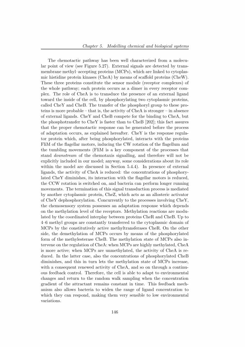
Chapter 5. Modelling chemical and biological systems
The chemotactic pathway has been well characterized from a molecu-lar point of view (see Figure 5.27). External signals are detected by trans-membrane methyl–accepting proteins (MCPs), which are linked to cytoplas-mic histidine protein kinases (CheA) by means of scaffold proteins (CheW).These three proteins constitute the sensor module (receptor complexes) ofthe whole pathway; each protein occurs as a dimer in every receptor com-plex. The role of CheA is to transduce the presence of an external ligandtoward the inside of the cell, by phosphorylating two cytoplasmic proteins,called CheY and CheB. The transfer of the phosphoryl group to these pro-teins is more probable – that is, the activity of CheA is stronger – in absenceof external ligands. CheY and CheB compete for the binding to CheA, butthe phosphotransfer to CheY is faster than to CheB [202]; this fact assuresthat the proper chemotactic response can be generated before the processof adaptation occurs, as explained hereafter. CheY is the response regula-tor protein which, after being phosphorylated, interacts with the proteinsFliM of the flagellar motors, inducing the CW rotation of the flagellum andthe tumbling movements (FliM is a key component of the processes thatstand downstream of the chemotaxis signalling, and therefore will not beexplicitly included in our model; anyway, some considerations about its rolewithin the model are discussed in Section 5.4.4). In presence of externalligands, the activity of CheA is reduced: the concentrations of phosphory-lated CheY diminishes, its interaction with the flagellar motors is reduced,the CCW rotation is switched on, and bacteria can perform longer runningmovements. The termination of this signal transduction process is mediatedby another cytoplasmic protein, CheZ, which acts as an allosteric activatorof CheY dephosphorylation. Concurrently to the processes involving CheY,the chemosensory system possesses an adaptation response which dependson the methylation level of the receptors. Methylation reactions are modu-lated by the coordinated interplay between proteins CheR and CheB. Up to4–6 methyl groups are constantly transferred to the cytoplasmic domain ofMCPs by the constitutively active methyltransferases CheR. On the otherside, the demethylation of MCPs occurs by means of the phosphorylatedform of the methylesterase CheB. The methylation state of MCPs also in-tervene on the regulation of CheA: when MCPs are highly methylated, CheAis more active; when MCPs are unmethylated, the activity of CheA is re-duced. In the latter case, also the concentrations of phosphorylated CheBdiminishes, and this in turn lets the methylation state of MCPs increase,with a consequent renewed activity of CheA, and so on through a continu-ous feedback control. Therefore, the cell is able to adapt to environmentalchanges and return to the random walk sampling when the concentrationgradient of the attractant remains constant in time. This feedback mech-anism also allows bacteria to widen the range of ligand concentration towhich they can respond, making them very sensible to low environmentalvariations.
146
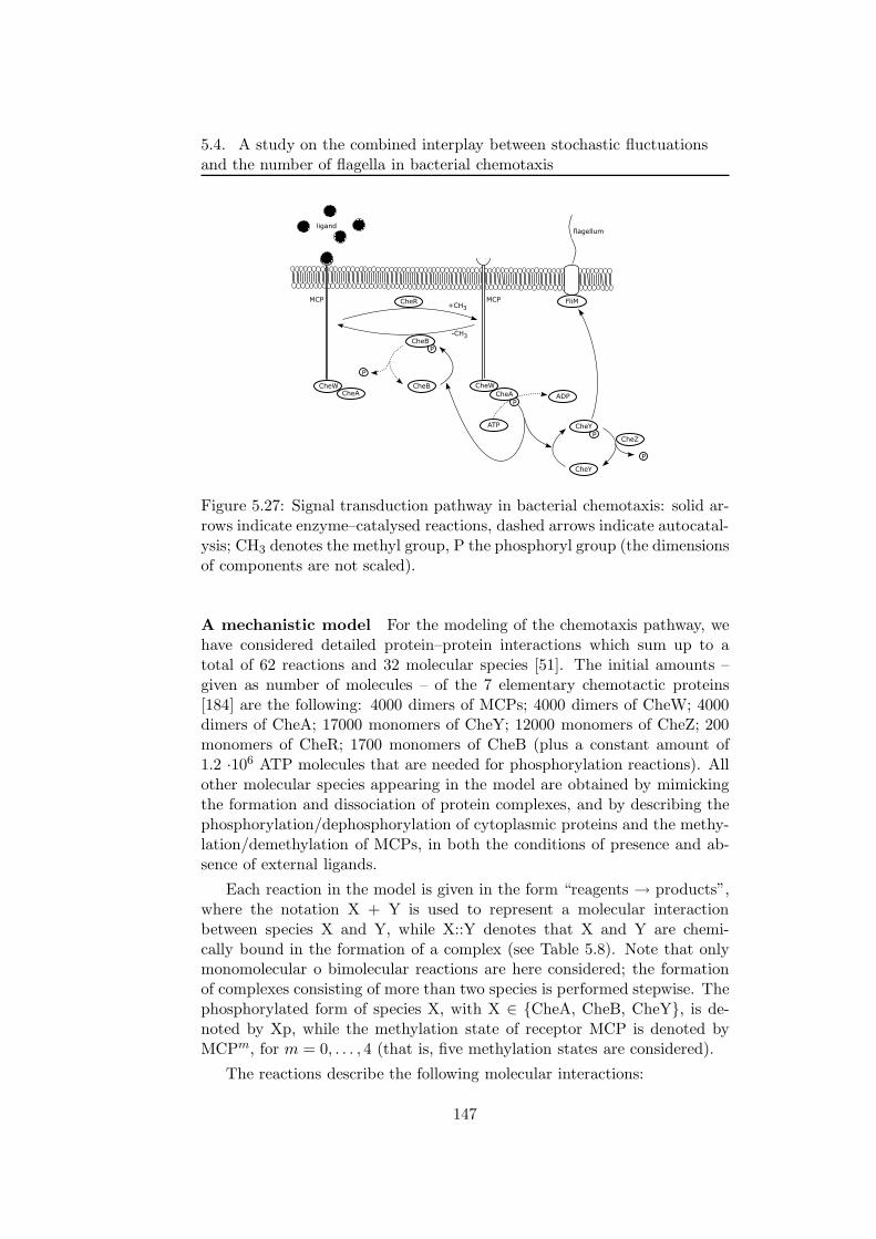
5.4. A study on the combined interplay between stochastic fluctuationsand the number of flagella in bacterial chemotaxis
Figure 5.27: Signal transduction pathway in bacterial chemotaxis: solid ar-rows indicate enzyme–catalysed reactions, dashed arrows indicate autocatal-ysis; CH3 denotes the methyl group, P the phosphoryl group (the dimensionsof components are not scaled).
A mechanistic model For the modeling of the chemotaxis pathway, wehave considered detailed protein–protein interactions which sum up to atotal of 62 reactions and 32 molecular species [51]. The initial amounts –given as number of molecules – of the 7 elementary chemotactic proteins[184] are the following: 4000 dimers of MCPs; 4000 dimers of CheW; 4000dimers of CheA; 17000 monomers of CheY; 12000 monomers of CheZ; 200monomers of CheR; 1700 monomers of CheB (plus a constant amount of1.2 ·106 ATP molecules that are needed for phosphorylation reactions). Allother molecular species appearing in the model are obtained by mimickingthe formation and dissociation of protein complexes, and by describing thephosphorylation/dephosphorylation of cytoplasmic proteins and the methy-lation/demethylation of MCPs, in both the conditions of presence and ab-sence of external ligands.
Each reaction in the model is given in the form “reagents → products”,where the notation X + Y is used to represent a molecular interactionbetween species X and Y, while X::Y denotes that X and Y are chemi-cally bound in the formation of a complex (see Table 5.8). Note that onlymonomolecular o bimolecular reactions are here considered; the formationof complexes consisting of more than two species is performed stepwise. Thephosphorylated form of species X, with X ∈ CheA, CheB, CheY, is de-noted by Xp, while the methylation state of receptor MCP is denoted byMCPm, for m = 0, . . . , 4 (that is, five methylation states are considered).
The reactions describe the following molecular interactions:
147
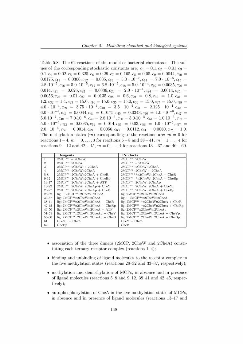
Chapter 5. Modelling chemical and biological systems
Table 5.8: The 62 reactions of the model of bacterial chemotaxis. The val-ues of the corresponding stochastic constants are: c1 = 0.1, c2 = 0.01, c3 =0.1, c4 = 0.02, c5 = 0.325, c6 = 0.29, c7 = 0.165, c8 = 0.05, c9 = 0.0044, c10 =0.0175, c11 = 0.0306, c12 = 0.035, c13 = 5.0 · 10−7, c14 = 7.0 · 10−6, c15 =2.8 ·10−5, c16 = 5.0 ·10−5, c17 = 6.8 ·10−5, c18 = 5.0 ·10−4, c19 = 0.0035, c20 =0.014, c21 = 0.025, c22 = 0.0336, c23 = 2.0 · 10−4, c24 = 0.0014, c25 =0.0056, c26 = 0.01, c27 = 0.0135, c28 = 0.6, c29 = 0.8, c30 = 1.0, c31 =1.2, c32 = 1.4, c33 = 15.0, c34 = 15.0, c35 = 15.0, c36 = 15.0, c37 = 15.0, c38 =4.0 · 10−4, c39 = 3.75 · 10−4, c40 = 3.5 · 10−4, c41 = 2.125 · 10−4, c42 =6.0 · 10−4, c43 = 0.0044, c44 = 0.0175, c45 = 0.0343, c46 = 1.0 · 10−8, c47 =5.0·10−7, c48 = 7.0·10−6, c49 = 2.8·10−5 , c50 = 5.0·10−5, c51 = 1.0·10−5, c52 =5.0 · 10−4, c53 = 0.0035, c54 = 0.014, c55 = 0.03, c56 = 1.0 · 10−5, c57 =2.0 · 10−4, c58 = 0.0014, c59 = 0.0056, c60 = 0.0112, c61 = 0.0080, c62 = 1.0.The methylation states (m) corresponding to the reactions are: m = 0 forreactions 1−4, m = 0, . . . , 3 for reactions 5−8 and 38−41, m = 1, . . . , 4 forreactions 9− 12 and 42− 45, m = 0, . . . , 4 for reactions 13− 37 and 46− 60.
Reagents Products
1 2MCPm + 2CheW 2MCPm::2CheW2 2MCPm::2CheW 2MCPm + 2CheW3 2MCPm::2CheW + 2CheA 2MCPm::2CheW::2CheA4 2MCPm::2CheW::2CheA 2MCPm::2CheW + 2CheA5-8 2MCPm::2CheW::2CheA + CheR 2MCPm+1::2CheW::2CheA + CheR9-12 2MCPm::2CheW::2CheA + CheBp 2MCPm−1::2CheW::2CheA + CheBp13-17 2MCPm::2CheW::2CheA + ATP 2MCPm::2CheW::2CheAp18-22 2MCPm::2CheW::2CheAp + CheY 2MCPm::2CheW::2CheA + CheYp23-27 2MCPm::2CheW::2CheAp + CheB 2MCPm::2CheW::2CheA + CheBp28-32 lig + 2MCPm::2CheW::2CheA lig::2MCPm::2CheW::2CheA33-37 lig::2MCPm::2CheW::2CheA lig + 2MCPm::2CheW::2CheA38-41 lig::2MCPm::2CheW::2CheA + CheR lig::2MCPm+1::2CheW::2CheA + CheR42-45 lig::2MCPm::2CheW::2CheA + CheBp lig::2MCPm−1::2CheW::2CheA + CheBp46-50 lig::2MCPm::2CheW::2CheA + ATP lig::2MCPm::2CheW::2CheAp51-55 lig::2MCPm::2CheW::2CheAp + CheY lig::2MCPm::2CheW::2CheA + CheYp56-60 lig::2MCPm::2CheW::2CheAp + CheB lig::2MCPm::2CheW::2CheA + CheBp61 CheYp + CheZ CheY + CheZ62 CheBp CheB
• association of the three dimers (2MCP, 2CheW and 2CheA) consti-tuting each ternary receptor complex (reactions 1–4);
• binding and unbinding of ligand molecules to the receptor complex inthe five methylation states (reactions 28–32 and 33–37, respectively);
• methylation and demethylation of MCPs, in absence and in presenceof ligand molecules (reactions 5–8 and 9–12, 38–41 and 42–45, respec-tively);
• autophosphorylation of CheA in the five methylation states of MCPs,in absence and in presence of ligand molecules (reactions 13–17 and
148

5.4. A study on the combined interplay between stochastic fluctuationsand the number of flagella in bacterial chemotaxis
46–50, respectively);
• phosphotransfer to CheY in different methylation states of MCPs, inabsence and in presence of ligand molecules (reactions 18–22 and 51–55, respectively);
• phosphotransfer to CheB in different methylation states of MCPs, inabsence and in presence of ligand molecules (reactions 23–27 and 56–60, respectively);
• dephosphorylation of CheYp and CheBp (reactions 61–62).
According to literature, the ternary receptor complex 2MCPm::2CheW::-2CheA is assumed to be stable for the duration of the signal transductionprocess [185]; moreover, the synthesis and degradation rates of all chemo-tactic proteins are assumed to occur at a much slower scale than the chemo-tactic response (hence, the reactions corresponding to these processes havenot been included in the model).
A stochastic constant is associated to each reaction, and it is neededto evaluate the probability of that reaction to occur, as explained in Sec-tion 1.1. The stochastic constants used for simulations are reported in thecaption of Table 5.8 (all values are expressed in sec−1). These values havebeen partly derived from literature [139], and partly tuned to account forthe following biological features [109, 124]: (1) the binding affinity of theligand is directly proportional to the methylation state of MCPs; (2) theligand–receptor binding reactions occur at a faster rate with respect to phos-phorylation and methylation/demethylation reactions; (3) the methylationand demethylation activities of CheR and CheBp are, respectively, inverselyand directly proportional to the methylation state of MCPs; (4) the rateof phosphotransfer from CheA to CheY and CheB depends on the rate ofautophosphorylation of CheA.
5.4.2 Stochastic simulations of chemotactic response regula-tor
In this section we show the results obtained for the chemotactic response reg-ulator protein, the phosphorylated CheY (CheYp), by analysing the systemunder different conditions.
As already said, all the simulations have been performed using the τ -DPP algorithm, setting the error control parameter ǫ = 0.03, as suggestedin [26]. All the simulations have been performed using a Personal Computerwith an Intel Core2 CPU (2.66 GHz) running Linux. The mean durationtime for one run, for the simulation of the dynamics of CheYp over 3000sec, is about 4–5 seconds (with the initial values of chemical amounts givenin Section 5.4.1 and the constants reported in Table 5.8). All the figures
149
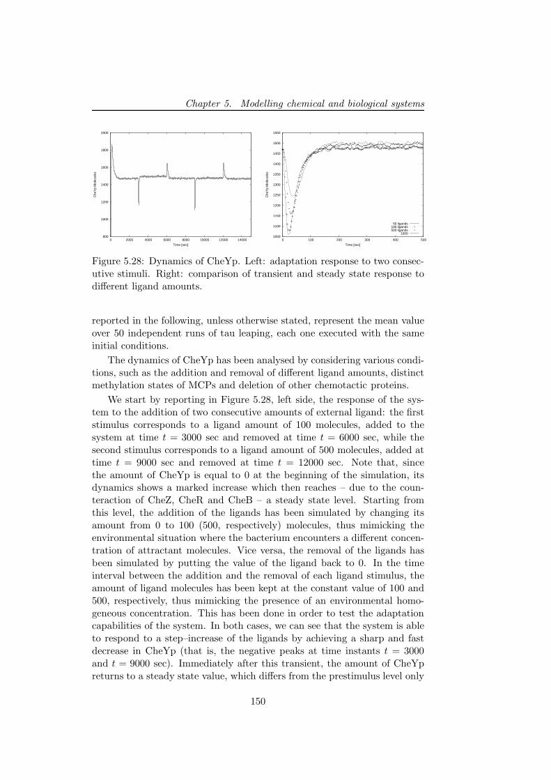
Chapter 5. Modelling chemical and biological systems
800
1000
1200
1400
1600
1800
2000
0 2000 4000 6000 8000 10000 12000 14000
Che
Yp
Mol
ecul
es
Time [sec]
1050
1100
1150
1200
1250
1300
1350
1400
1450
1500
1550
0 100 200 300 400 500
Che
Yp
Mol
ecul
es
Time [sec]
50 ligands100 ligands500 ligands
1000
Figure 5.28: Dynamics of CheYp. Left: adaptation response to two consec-utive stimuli. Right: comparison of transient and steady state response todifferent ligand amounts.
reported in the following, unless otherwise stated, represent the mean valueover 50 independent runs of tau leaping, each one executed with the sameinitial conditions.
The dynamics of CheYp has been analysed by considering various condi-tions, such as the addition and removal of different ligand amounts, distinctmethylation states of MCPs and deletion of other chemotactic proteins.
We start by reporting in Figure 5.28, left side, the response of the sys-tem to the addition of two consecutive amounts of external ligand: the firststimulus corresponds to a ligand amount of 100 molecules, added to thesystem at time t = 3000 sec and removed at time t = 6000 sec, while thesecond stimulus corresponds to a ligand amount of 500 molecules, added attime t = 9000 sec and removed at time t = 12000 sec. Note that, sincethe amount of CheYp is equal to 0 at the beginning of the simulation, itsdynamics shows a marked increase which then reaches – due to the coun-teraction of CheZ, CheR and CheB – a steady state level. Starting fromthis level, the addition of the ligands has been simulated by changing itsamount from 0 to 100 (500, respectively) molecules, thus mimicking theenvironmental situation where the bacterium encounters a different concen-tration of attractant molecules. Vice versa, the removal of the ligands hasbeen simulated by putting the value of the ligand back to 0. In the timeinterval between the addition and the removal of each ligand stimulus, theamount of ligand molecules has been kept at the constant value of 100 and500, respectively, thus mimicking the presence of an environmental homo-geneous concentration. This has been done in order to test the adaptationcapabilities of the system. In both cases, we can see that the system is ableto respond to a step–increase of the ligands by achieving a sharp and fastdecrease in CheYp (that is, the negative peaks at time instants t = 3000and t = 9000 sec). Immediately after this transient, the amount of CheYpreturns to a steady state value, which differs from the prestimulus level only
150
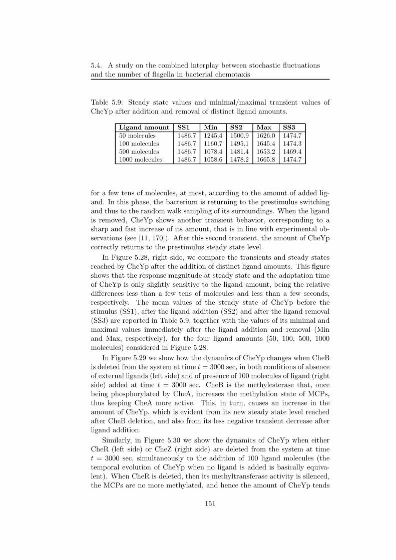
5.4. A study on the combined interplay between stochastic fluctuationsand the number of flagella in bacterial chemotaxis
Table 5.9: Steady state values and minimal/maximal transient values ofCheYp after addition and removal of distinct ligand amounts.
Ligand amount SS1 Min SS2 Max SS350 molecules 1486.7 1245.4 1500.9 1626.0 1474.7100 molecules 1486.7 1160.7 1495.1 1645.4 1474.3500 molecules 1486.7 1078.4 1481.4 1653.2 1469.41000 molecules 1486.7 1058.6 1478.2 1665.8 1474.7
for a few tens of molecules, at most, according to the amount of added lig-and. In this phase, the bacterium is returning to the prestimulus switchingand thus to the random walk sampling of its surroundings. When the ligandis removed, CheYp shows another transient behavior, corresponding to asharp and fast increase of its amount, that is in line with experimental ob-servations (see [11, 170]). After this second transient, the amount of CheYpcorrectly returns to the prestimulus steady state level.
In Figure 5.28, right side, we compare the transients and steady statesreached by CheYp after the addition of distinct ligand amounts. This figureshows that the response magnitude at steady state and the adaptation timeof CheYp is only slightly sensitive to the ligand amount, being the relativedifferences less than a few tens of molecules and less than a few seconds,respectively. The mean values of the steady state of CheYp before thestimulus (SS1), after the ligand addition (SS2) and after the ligand removal(SS3) are reported in Table 5.9, together with the values of its minimal andmaximal values immediately after the ligand addition and removal (Minand Max, respectively), for the four ligand amounts (50, 100, 500, 1000molecules) considered in Figure 5.28.
In Figure 5.29 we show how the dynamics of CheYp changes when CheBis deleted from the system at time t = 3000 sec, in both conditions of absenceof external ligands (left side) and of presence of 100 molecules of ligand (rightside) added at time t = 3000 sec. CheB is the methylesterase that, oncebeing phosphorylated by CheA, increases the methylation state of MCPs,thus keeping CheA more active. This, in turn, causes an increase in theamount of CheYp, which is evident from its new steady state level reachedafter CheB deletion, and also from its less negative transient decrease afterligand addition.
Similarly, in Figure 5.30 we show the dynamics of CheYp when eitherCheR (left side) or CheZ (right side) are deleted from the system at timet = 3000 sec, simultaneously to the addition of 100 ligand molecules (thetemporal evolution of CheYp when no ligand is added is basically equiva-lent). When CheR is deleted, then its methyltransferase activity is silenced,the MCPs are no more methylated, and hence the amount of CheYp tends
151
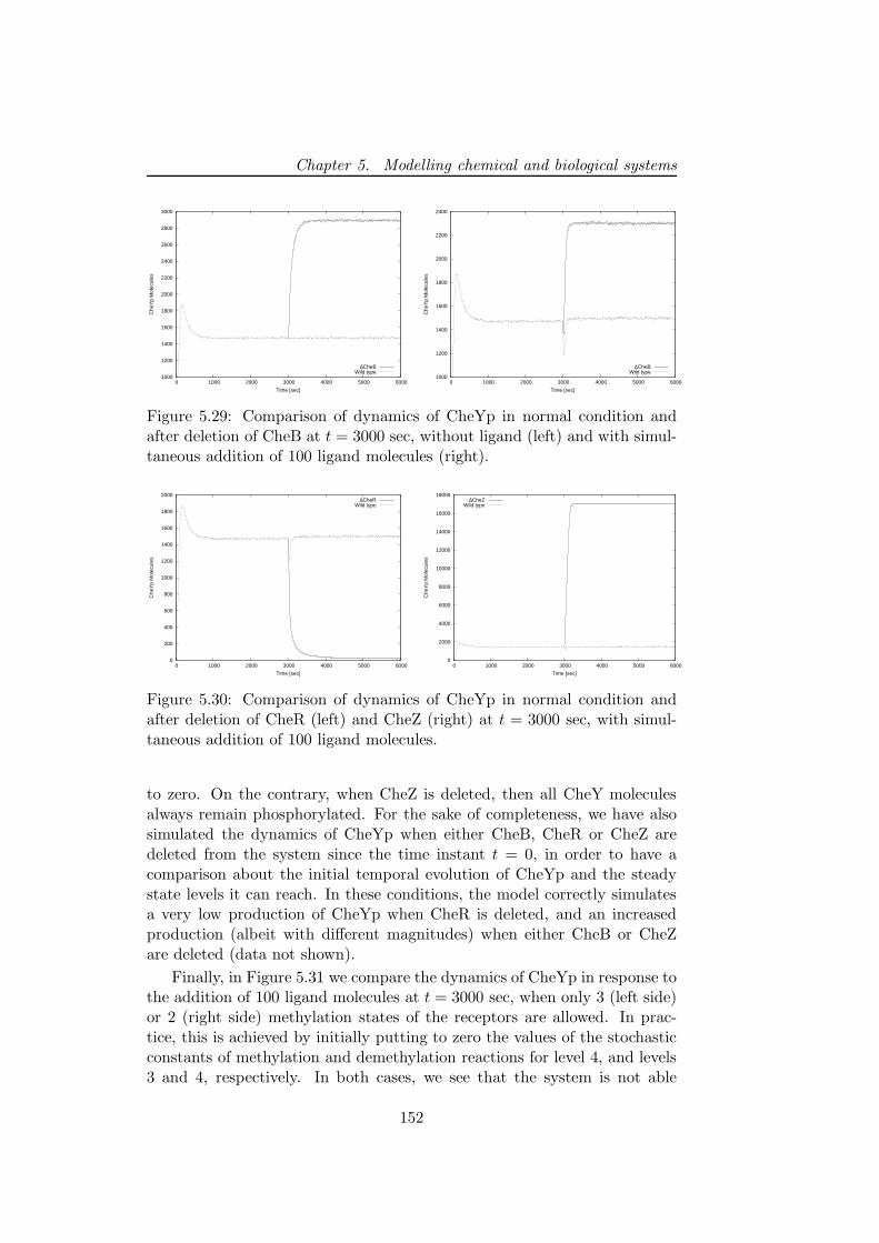
Chapter 5. Modelling chemical and biological systems
1000
1200
1400
1600
1800
2000
2200
2400
2600
2800
3000
0 1000 2000 3000 4000 5000 6000
Che
Yp
Mol
ecul
es
Time [sec]
∆CheBWild type
1000
1200
1400
1600
1800
2000
2200
2400
0 1000 2000 3000 4000 5000 6000
Che
Yp
Mol
ecul
es
Time [sec]
∆CheBWild type
Figure 5.29: Comparison of dynamics of CheYp in normal condition andafter deletion of CheB at t = 3000 sec, without ligand (left) and with simul-taneous addition of 100 ligand molecules (right).
0
200
400
600
800
1000
1200
1400
1600
1800
2000
0 1000 2000 3000 4000 5000 6000
Che
Yp
Mol
ecul
es
Time [sec]
∆CheRWild type
0
2000
4000
6000
8000
10000
12000
14000
16000
18000
0 1000 2000 3000 4000 5000 6000
Che
Yp
Mol
ecul
es
Time [sec]
∆CheZWild type
Figure 5.30: Comparison of dynamics of CheYp in normal condition andafter deletion of CheR (left) and CheZ (right) at t = 3000 sec, with simul-taneous addition of 100 ligand molecules.
to zero. On the contrary, when CheZ is deleted, then all CheY moleculesalways remain phosphorylated. For the sake of completeness, we have alsosimulated the dynamics of CheYp when either CheB, CheR or CheZ aredeleted from the system since the time instant t = 0, in order to have acomparison about the initial temporal evolution of CheYp and the steadystate levels it can reach. In these conditions, the model correctly simulatesa very low production of CheYp when CheR is deleted, and an increasedproduction (albeit with different magnitudes) when either CheB or CheZare deleted (data not shown).
Finally, in Figure 5.31 we compare the dynamics of CheYp in response tothe addition of 100 ligand molecules at t = 3000 sec, when only 3 (left side)or 2 (right side) methylation states of the receptors are allowed. In prac-tice, this is achieved by initially putting to zero the values of the stochasticconstants of methylation and demethylation reactions for level 4, and levels3 and 4, respectively. In both cases, we see that the system is not able
152
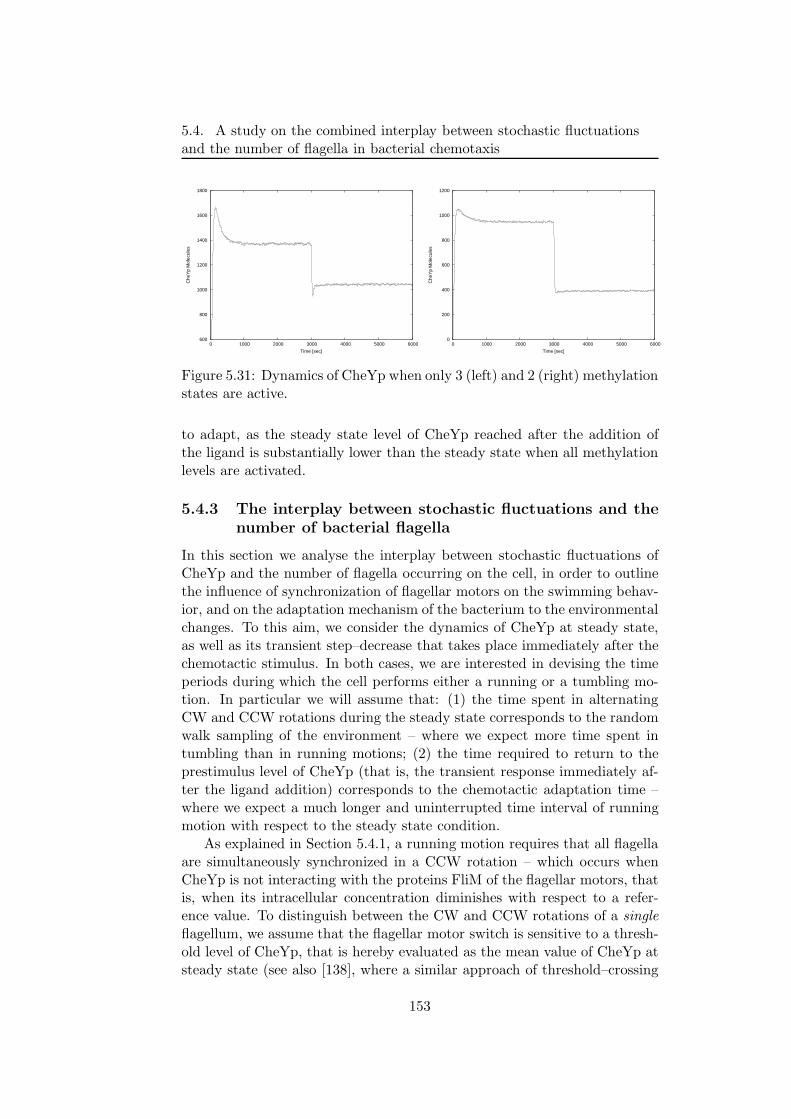
5.4. A study on the combined interplay between stochastic fluctuationsand the number of flagella in bacterial chemotaxis
600
800
1000
1200
1400
1600
1800
0 1000 2000 3000 4000 5000 6000
Che
Yp
Mol
ecul
es
Time [sec]
0
200
400
600
800
1000
1200
0 1000 2000 3000 4000 5000 6000
Che
Yp
Mol
ecul
es
Time [sec]
Figure 5.31: Dynamics of CheYp when only 3 (left) and 2 (right) methylationstates are active.
to adapt, as the steady state level of CheYp reached after the addition ofthe ligand is substantially lower than the steady state when all methylationlevels are activated.
5.4.3 The interplay between stochastic fluctuations and thenumber of bacterial flagella
In this section we analyse the interplay between stochastic fluctuations ofCheYp and the number of flagella occurring on the cell, in order to outlinethe influence of synchronization of flagellar motors on the swimming behav-ior, and on the adaptation mechanism of the bacterium to the environmentalchanges. To this aim, we consider the dynamics of CheYp at steady state,as well as its transient step–decrease that takes place immediately after thechemotactic stimulus. In both cases, we are interested in devising the timeperiods during which the cell performs either a running or a tumbling mo-tion. In particular we will assume that: (1) the time spent in alternatingCW and CCW rotations during the steady state corresponds to the randomwalk sampling of the environment – where we expect more time spent intumbling than in running motions; (2) the time required to return to theprestimulus level of CheYp (that is, the transient response immediately af-ter the ligand addition) corresponds to the chemotactic adaptation time –where we expect a much longer and uninterrupted time interval of runningmotion with respect to the steady state condition.
As explained in Section 5.4.1, a running motion requires that all flagellaare simultaneously synchronized in a CCW rotation – which occurs whenCheYp is not interacting with the proteins FliM of the flagellar motors, thatis, when its intracellular concentration diminishes with respect to a refer-ence value. To distinguish between the CW and CCW rotations of a singleflagellum, we assume that the flagellar motor switch is sensitive to a thresh-old level of CheYp, that is hereby evaluated as the mean value of CheYp atsteady state (see also [138], where a similar approach of threshold–crossing
153
Chapter 5. Modelling chemical and biological systems
mechanism for motor switching was tested, albeit that work considered onlysingle flagellum and did not propose any investigation on the simultane-ous coordination of many flagella). When the amount of CheYp is belowthis threshold, each flagellum is rotating CCW, while when the amount ofCheYp is above the threshold, each flagellum is rotating CW. In what fol-lows, we make a one–to–one correspondence between the behavior of a singleflagellum and one temporal evolution of CheYp generated by one run of theτ -DPP algorithm, that is, we consider a different and independent stochasticsimulation for each and every flagellum (albeit starting from the same initialconditions). To determine the synchronization of all flagella, that will in-duce a running motion, we therefore need to identify the time instants whenall flagella are rotating CCW, that is, to select the time intervals when allthe temporal evolutions of CheYp are below the fixed threshold.
Formally, we proceed as follows. Let n = 1, . . . , 10 be the number offlagella f1, . . . , fn whose influence we want to test, and let si, i = 1, . . . , n,be the temporal series of CheYp (generated by a single τ -DPP run) as-sociated to each fi. For any fixed value of n, the total time of the sim-ulation considered to generate the dynamics of CheYp is the same forall si. This simulation time, hereby denoted by ∆tsim, is chosen longenough to have statistical significance for the analysis performed below (e.g.∆tsim = 40000, 60000, 120000 sec for n = 1, 5, 10, respectively). The thresh-old for CheYp is evaluated in the following way: we choose an initial timeinstant at the steady state level – distant enough from the step decreaseof CheYp after ligand addition, i.e. 1000 sec afterwards – and then, start-ing from this instant and till the end of ∆tsim, we calculate the mean valueµi =< si > for each si. Then, we define a common threshold µ for all flagellasuch that µ = 1
n
∑ni=1 µi. This threshold is considered as the reference value
also for the portion of the CheYp dynamics corresponding to the transientdecrease after ligand addition. In Figure 5.32, top panel on the left side, weshow a part of ∆tsim over a single simulation of CheYp, where both the ini-tial transient response and the stochastic fluctuations around the thresholdare evidenced. For all the results discussed below, the different values of µhave been found to be approximatively equal to 1480 molecules.
The next step consists in detecting, for each fi, the time intervals duringwhich the amount of CheYp remains below µ, each one of these intervalscorresponding to a CCW rotation time interval of that flagellum. Namely,for each si we identify the time intervals ∆ttrue ⊆ ∆tsim such that ∆ttrue =t ∈ ∆tsim | si(t) − µ ≤ 0. Note that this simple mechanism of singlethreshold-crossing could be extended to consider more complex situations– e.g., a double threshold-crossing mode can be assumed – whereby onesimply asks for analogous conditions to be satisfied. Similarly, for each si
we can locate the complementary time intervals ∆tfalse ⊆ ∆tsim such that∆tfalse = t ∈ ∆tsim | si(t)−µ > 0; these intervals correspond to the timethat each flagellum fi spends in a CW rotation. Stated in other terms, we
154
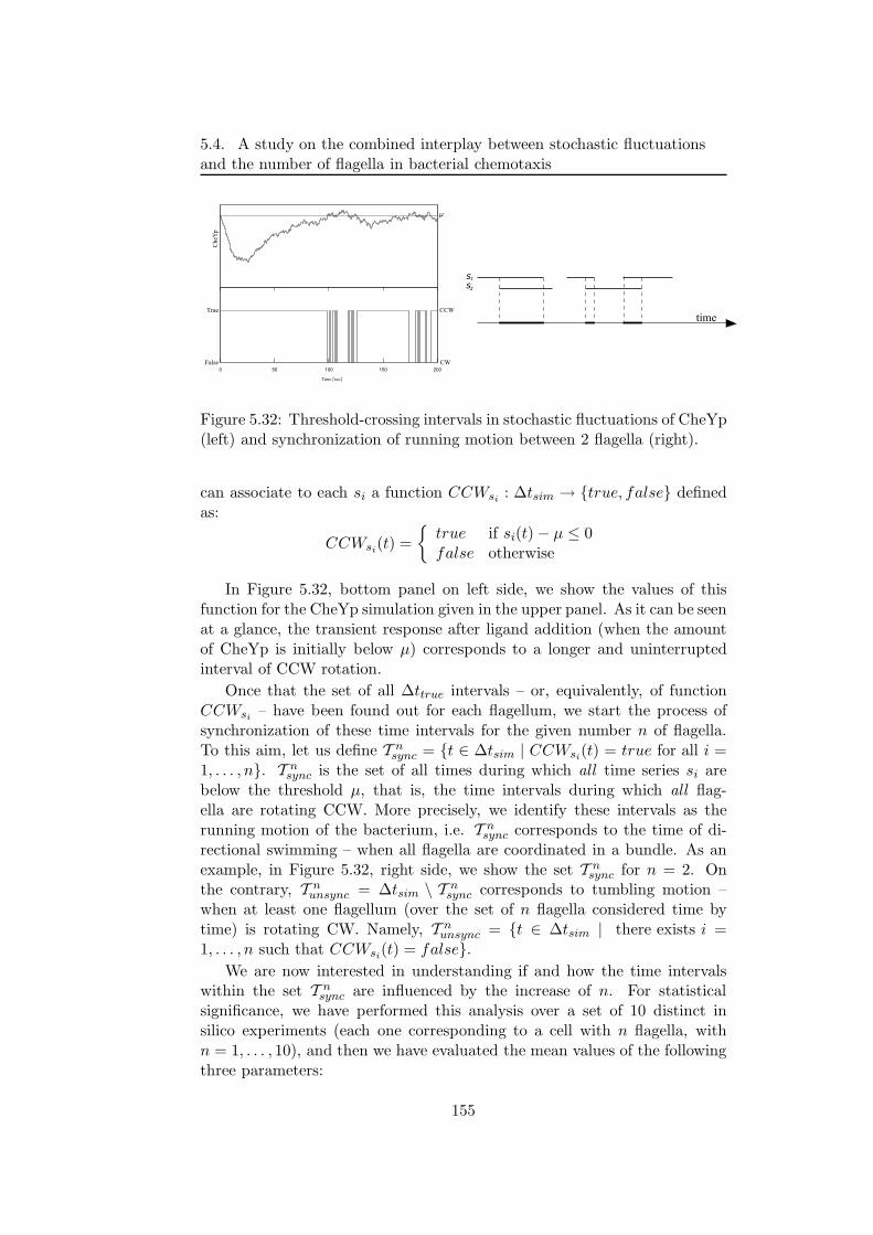
5.4. A study on the combined interplay between stochastic fluctuationsand the number of flagella in bacterial chemotaxis
Figure 5.32: Threshold-crossing intervals in stochastic fluctuations of CheYp(left) and synchronization of running motion between 2 flagella (right).
can associate to each si a function CCWsi: ∆tsim → true, false defined
as:
CCWsi(t) =
true if si(t) − µ ≤ 0false otherwise
In Figure 5.32, bottom panel on left side, we show the values of thisfunction for the CheYp simulation given in the upper panel. As it can be seenat a glance, the transient response after ligand addition (when the amountof CheYp is initially below µ) corresponds to a longer and uninterruptedinterval of CCW rotation.
Once that the set of all ∆ttrue intervals – or, equivalently, of functionCCWsi
– have been found out for each flagellum, we start the process ofsynchronization of these time intervals for the given number n of flagella.To this aim, let us define T n
sync = t ∈ ∆tsim | CCWsi(t) = true for all i =
1, . . . , n. T nsync is the set of all times during which all time series si are
below the threshold µ, that is, the time intervals during which all flag-ella are rotating CCW. More precisely, we identify these intervals as therunning motion of the bacterium, i.e. T n
sync corresponds to the time of di-rectional swimming – when all flagella are coordinated in a bundle. As anexample, in Figure 5.32, right side, we show the set T n
sync for n = 2. Onthe contrary, T n
unsync = ∆tsim \ T nsync corresponds to tumbling motion –
when at least one flagellum (over the set of n flagella considered time bytime) is rotating CW. Namely, T n
unsync = t ∈ ∆tsim | there exists i =1, . . . , n such that CCWsi
(t) = false.
We are now interested in understanding if and how the time intervalswithin the set T n
sync are influenced by the increase of n. For statisticalsignificance, we have performed this analysis over a set of 10 distinct insilico experiments (each one corresponding to a cell with n flagella, withn = 1, . . . , 10), and then we have evaluated the mean values of the followingthree parameters:
155
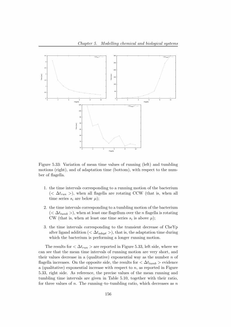
Chapter 5. Modelling chemical and biological systems
0
0.5
1
1.5
2
2.5
3
3.5
0 2 4 6 8 10
Tim
e [s
ec]
Flagella
< ∆ trun >
0
50
100
150
200
250
300
0 2 4 6 8 10
Tim
e [s
ec]
Flagella
< ∆ ttumb >
70
75
80
85
90
95
100
105
0 2 4 6 8 10
Tim
e [s
ec]
Flagella
< ∆ tadapt >
Figure 5.33: Variation of mean time values of running (left) and tumblingmotions (right), and of adaptation time (bottom), with respect to the num-ber of flagella.
1. the time intervals corresponding to a running motion of the bacterium(< ∆trun >), when all flagella are rotating CCW (that is, when alltime series si are below µ);
2. the time intervals corresponding to a tumbling motion of the bacterium(< ∆ttumb >), when at least one flagellum over the n flagella is rotatingCW (that is, when at least one time series si is above µ);
3. the time intervals corresponding to the transient decrease of CheYpafter ligand addition (< ∆tadapt >), that is, the adaptation time duringwhich the bacterium is performing a longer running motion.
The results for < ∆trun > are reported in Figure 5.33, left side, where wecan see that the mean time intervals of running motion are very short, andtheir values decrease in a (qualitative) exponential way as the number n offlagella increases. On the opposite side, the results for < ∆ttumb > evidencea (qualitative) exponential increase with respect to n, as reported in Figure5.33, right side. As reference, the precise values of the mean running andtumbling time intervals are given in Table 5.10, together with their ratio,for three values of n. The running–to–tumbling ratio, which decreases as n
156
5.4. A study on the combined interplay between stochastic fluctuationsand the number of flagella in bacterial chemotaxis
Table 5.10: Values of mean time intervals for running, tumbling and adap-tation.
n 〈∆trun〉 (sec) 〈∆ttumb〉 (sec) 〈∆trun〉/〈∆ttumb〉 〈∆tadapt〉 (sec)1 3.102 3.062 1.013 104.05 0.606 18.73 0.032 73.4810 0.310 297.4 0.001 72.22
increases, highlights the relevance of the number of flagella and the necessityof their synchronization with respect to the chemotactic behavior of thebacterium. That is, we see that for n = 1 the time spent in running ortumbling motions is approximatively equivalent, but if coordination amongmany flagella (n = 10) has to take place, then the running motions arehighly reduced with respect to tumbling motions, which is in agreementwith biological expectations.
The results for < ∆tadapt > are reported in Figure 5.33, bottom, andin Table 5.10. In this case, it is not possible to recognize a simple functionfor the curve progress, and we see that the variation of the time intervalsis within a range of a few tens of seconds. Once more, this result seems tobe in agreement with biological expectations, as the response of the bac-terium to an environmental change (i.e. the presence of ligands) should notbe strictly dependent on the number of flagella that are present on its sur-face, otherwise the chemotactic pathway would not guarantee an appropriateadaptation mechanism, independently from the variation of the number offlagella among individuals in a population of cells.
5.4.4 Discussion
We have proposed a very detailed mechanistic model of the bacterial chemo-taxis pathway that takes into account all proteins, and their respective in-teractions, involved in both signalling and response. In particular, all post-translational modifications of proteins, such as methylation and phosphory-lation, have been considered because of their relevant roles in the feedbackcontrol mechanisms governing this pathway. By exploiting the τ -DPP al-gorithm, we have investigated the dynamics of the pivotal protein involvedin chemotaxis, CheYp, under different conditions, such as the deletion ofother chemotactic proteins, the addition of distinct amounts of external lig-and, the effect of different methylation states. Then, we have investigatedthe possible influence of stochastic fluctuations of CheYp with respect toan increasing number of flagella in the individual bacterium. Namely, wehave defined a procedure to identify the synchronization of CCW rotationsof all flagella, and then we have compared the mean time intervals of run-ning and tumbling motions of the cell, as well as of adaptation times to
157
Chapter 5. Modelling chemical and biological systems
ligand addition, according to the different numbers of flagella. We haveshown that the running–to–tumbling ratio highlights the relevance of thenumber of flagella, and the necessity of their synchronization with respectto the chemotactic behavior of the bacterium. Moreover, we have shownthat the adaptation time does not seem to be strongly influenced by thevarying number of flagella in distinct individual cells.
Concerning the analysis of the interplay between CheYp fluctuationsand the number of flagella, another aspect could be investigated, such asthe influence of the amount of external ligands on the adaptation times (inSection 5.4.3, in fact, only the addition of 1000 ligands was used to executeall simulations). We will consider this matter in a forthcoming extension ofthis work. In addition, other relevant biological aspects of chemotaxis, thatstand downstream of the signalling process, might represent valuable pointsto be included in a future study. For instance, it is known that each flagel-lar motor switch–complex is constituted by a group of proteins, called FliM,FliN, FliG (assembled in a ring), and by the torque–generating complexes,called MotA and MotB. In E. coli, a typical flagellar ring contains 34 copiesof FliM, each of which can bind one copy of CheYp. In [53] it is suggestedthat binding of CheYp to FliM modifies the displacement of protein FliG,which directly interacts with the Mot complexes and therefore modulatesthe switch state of the flagellum. Moreover, flagellar motor switching hasbeen found to be highly sensitive to the concentration of CheYp (having aHill coefficient ≈ 10), though the binding of CheYp to FliM has a low levelof cooperativity (Hill coefficient ≈ 1). In [53], the hypothesis that CheYpcan interact more favourably with the FliM displaced in the CW orientation,than those in the CCW orientation, is put forward. In [181], in addition,the following mechanism is considered for the control of flagellar motor bymeans of CheYp: the number of CheYp molecules bound to FliM deter-mines the probability of CW or CCW rotation, while the switch is thrownby thermal fluctuations. In other words, CheYp only changes the stabili-ties of the two rotational states, by shifting the energy level of CCW–stateup and of CW–state down, by a magnitude that is directly proportional tothe number of bound molecules. Therefore, interesting questions related tostochastic fluctuations of CheYp, that might be coupled with the investi-gation on the number of cellular flagella, are: how many FliM proteins ateach flagellar switch have to be occupied by CheYp in order to generate theCW rotation [21]? What is the corresponding probability of throwing thereversal switch? Can a double–threshold crossing mechanism [21] be moresuitable to effectively detect the CW and CCW rotational states?
Nonetheless, other related features might be relevant points for a furtherextension of this work. For instance, the model does not take into accountthe diffusion processes of molecules inside the volume where reactions occur.Though, the gradient of CheYp that can be present inside the cytoplasm –due to the diffusion from the area of its phosphorylation (close to chemotac-
158
5.4. A study on the combined interplay between stochastic fluctuationsand the number of flagella in bacterial chemotaxis
tic receptors) to the area of its activity (around the flagellar motors) – canbe a significant aspect in chemotaxis, together with the localization of CheZ(that controls the dephosphorylation of CheYp) and of the flagella aroundthe cell [110].
We believe that the definition of detailed mechanistic models, like theone proposed here for chemotaxis, and the use of efficient tools for the anal-ysis of stochastic processes in individual cells, can be a good benchmark toinvestigate the combined roles of many interplaying biological factors. Withthis perspective, the development of formal methods specifically devised forthe analysis of properties of stochastic systems represents indeed a majorhot topic research in biological modeling.
159

Chapter 5. Modelling chemical and biological systems
160
Chapter 6
The role of parameters inchemical and biologicalsystems
The modelling of biological systems requires the knowledge of many numer-ical factors, like the concentrations of molecular species or reaction rates,which represent an indispensable quantitative information to perform com-putational investigations of the system behavior. Unfortunately, the exper-imental values related to molecular quantities and rate constants are oftennot available or inaccurate [173]. This lack of information has led to thedevelopment of different techniques, based on local or global optimisationmethods, in order to estimate the unknown parameters [137].
In addition, once that the calibration of the parameters of a systems hasbeen done, it is interesting to study and analyse the effect of the combinationof different values of the parameters by means of ad hoc techniques (e.g.parameter sweep) that are suitable to the exploration of these very largeand complex research spaces. Parameter sweep can be realised by executinga very large number of simulations, each one corresponding to a differentparametrisation of the analysed system, in order to test its robustness andto find its crucial points.
In this chapter, we will first present the issue of parameter estimation forbiochemical systems (Section 6.1), together with a brief description of theoptimisation techniques that are already present in literature for this scope.Afterwards, we recall the basic definition of parameter sweep application(Section 6.2) emphasising its suitability for the exploration of the parametersspace of biological systems.
Both parameter estimation and parameter sweep require the definition ofan appropriate fitness function, in order to quantify the quality of a partic-ular set of parameters. To be more precise, this function is used to measurethe “difference” between the estimated dynamics, that is, the behavior ob-
161
Chapter 6. The role of parameters in chemical and biological systems
tained through a simulation using the set of parameters under investigation,and a target dynamics, which represents a known behaviour of the system.The fitness function used hereby, will be described in Section 6.3.
In Section 6.4, we show how we can tackle the problem of estimating theunknown parameters of stochastic biochemical systems by means of two opti-mization heuristics, genetic algorithms and particle swarm optimization [15].Their performances are tested and compared on two basic kinetics schemes:the Michaelis–Menten equation and the Brussellator. The experimental re-sults suggest that particle swarm optimization is a suitable method for thisproblem. The set of parameters estimated by particle swarm optimizationallows us to reliably reconstruct the dynamics of the Michaelis–Menten sys-tem and of the Brussellator in the oscillating regime.
Finally, in Section 6.5 we present a possible implementation of parametersweep application obtained by distributing a number of stochastic simula-tions on the EGEE project grid platform [140]. As a case study, we present aparameter sweep application for a stochastic model of bacterial chemotaxiscomposed of 59 reactions and 31 chemical species. In order to analyse theeffect of parameter variation over the dynamics of this system, we have per-formed a large number of simulations to explore the 59-dimensional space ofits stochastic constants, and considered the temporal evolution of a pivotalprotein as the reference dynamics. The performance and the results ob-tained from the different parameter sweep applications executed are finallydiscussed.
162
6.1. Parameter estimation of biochemical systems
6.1 Parameter estimation of biochemical systems
In computational investigation of biochemical systems, the first step consistsin understanding the system structure (that is, the molecular species andcompartments involved in the system, their localisation and topology, etc.)and in developing a model to describe the interactions among the systemcomponents. The second stage corresponds to the study of the dynamics ofthe system, under different conditions, in order to yield useful predictionsabout any unknown interactions which can take place within the system.To achieve these tasks, it is important to identify the system structure aswell as the set of parameters, because both are needed to analyse the be-havior of such systems. The final stage consists in comparing the obtainedcomputational results with the experimental results, in order to validate thedeveloped model [101].
One of the most challenging step in this process, which is usually dueto the non–linearity of these systems, is the estimation of the large set ofnumerical parameters that they contain. These parameters are: molecularamounts, binding constants, transcription rates, translation rates, chemi-cal reaction rates, degradation rates, diffusion rates, etc. Except for specialcases where the experimental values of these factor can be found in literature,they are often not available or inaccurate, since carrying out their measure-ments in vivo can be tangling or even impossible [173]. In a few cases, thevalues of some parameters of a given system can be estimated either from invitro experiments (by fitting the dynamics derived through equations basedon mass-action law against the concentration time series that result fromthese measurements), or by assuming some analogies with similar processesor organisms for which more experimental data are available. In general, itis exactly the lack and the inaccuracy of these information that bring aboutthe problem of assigning the correct values to all parameters, in order toreproduce the expected dynamics in the best possible way.
The parameter estimation issue, also called inverse problem [126], con-sists in the calibration of the unknown system’s parameters by means ofoptimisation techniques. It is called “inverse” because it is the oppositeof the “forward” problem of the simulation of a system’s dynamics. Theinverse problem requires methods that can combine simulation techniqueswith optimization algorithms, capable of searching global optima in large(and complex) multi–dimensional spaces.
In general, the calibration of the parameters values can be tackled ac-cording to the following simple procedure [127]:
1. Simulate the model with the given set of parameters;
2. Compare the known experimental time course with the simulation out-come;
163
Chapter 6. The role of parameters in chemical and biological systems
3. If the difference between these two dynamics is “small enough”, thenstop, otherwise adjust the parameters of the model;
4. Go back to step 1.
Step 1 of the procedure consists in the simulation of the model, which isthe “inverse” problem of optimisation. During this step, given a set of fixedparameters, the dynamics of the system is described. Note that, usually,in the first iteration of this procedure, the initial values for the parametersare randomly chosen according to the chosen optimisation technique. After-wards, the experimental data (if available) or a generic “reference dynamics”is compared to the results of the simulation in order to quantify the quality ofthe set of parameters previously assigned to the model. This task is accom-plished by computing the value of a fitness function. During step 3, the valueof the fitness function is checked in order to decide if the set of parametersneeds further refinements, or if it is acceptable according to some specifiedcriterion. In the first case, the values of the parameters are adjusted usingan optimisation technique, such as e.g. hill climbing, simulated annealing,genetic algorithms or particle swarm optimizer, and another iteration of theprocedure is executed. In the second case, the procedure terminates.
In general, the inverse problem is complicated by the non–linearity of thesystem’s dynamics which is very often multimodal (i.e. nonconvex) [127].The first attempt to tackle this kind of optimisation problems, the so–calledmultistart strategy, has been presented in [83]. This method consists in therepeated application of local methods, starting from a number of differentinitial sets of parameters for the analysed model. However, this approach isnot suitable for real applications because of its inefficiency; as a matter offact, when many starting points are used, the same minimum is determinedseveral times. Moreover, the execution of a large number of instances of thismethod is very time consuming.
The limitations of local methods lead to the application of global op-timisation methods in order to improve the efficiency and the robustness.In particular, in [127], the parameter estimation of the mechanism of irre-versible inhibition of HIV proteinase has been presented, and the best resultshave been obtained by using the simulated annealing method. However, alsoin this case the main drawback is represented by the computational time re-quired by the execution of this procedure.
Several different stochastic optimisation methods, applied to the param-eter estimation of a large three-step pathway, that is, a case study consistingin the optimisation of 36 kinetic parameters, have been compared in [125].The best performing method found was the evolutionary programming, sincethe solution obtained by the application of this procedure allowed to de-scribe the correct dynamics of the analysed system, while other methodsfailed. More recently, in [137], several global optimisation methods have
164
6.2. Parameter sweep application
been applied for the calibration of 36 parameters of a benchmark model.The most suitable method for the solution of the inverse problem, amongthose considered by the authors, was the evolution strategy using stochasticranking (SRES), presented in [178]. SRES is an evolutionary optimisationalgorithm that uses stochastic ranking as constraint handling technique, amethod that adjusts the balance between the objective and the penaltyfunctions automatically during the evolutionary search.
The main disadvantage of these global optimisation methods is the timerequired to perform a computation; however, it is well known that the meth-ods cited above can be easily parallelised, thus reducing the computationaltime needed to obtain good results.
The method for the parameter estimation that we will propose in thefollowing sections exploits two population based optimisation heuristic: ge-netic algorithms and particle swarm optimizer. These methods are suitablefor the optimisation of sets of real values, like the parameters of biochemicalsystems, and their efficiency in the exploration of the parameter space hasbeen proved by many applications. Moreover, our approach for the parame-ter estimation, like those presented above, can be parallelised, for instance,by distributing the computation of the fitness functions (which is usuallythe most time consuming task of the procedure) on a cluster.
6.2 Parameter sweep application
The behaviour of biochemical models is mainly influenced by the initialconditions, i.e. the molecular quantities, and by the rate constants valuesassigned to the chemical reactions. Real models are usually composed ofa large number of chemical species which interact through many chemicalreactions, hence, the space constituted by all possible combinations of valuesof the parameters has a high number of dimensions. Therefore, the explo-ration of such kind of spaces, to the aim of quantifying the influence of theparameter values on the system dynamics, is a hard task.
There exist many different techniques suitable for this kind of analysis.For instance, steady state analysis concerns the identification of points in thespace of reachable states, where the dynamical system is fixed (e.g. wherethe behaviour of the system is constant over time); bifurcation analysis stud-ies the qualitative variation of the dynamics (e.g. transition from oscillatingto non oscillating regime) as a consequence of the variation of the parame-ters; sensitivity analysis relates the uncertainty of the input of a model (i.e.variations in parameters and initial conditions) to its output (namely, theresulting behaviour); and parameter sweep application (PSA) explore theparameters space of a system by means of independent experiments.
Among the techniques cited here, PSA represents one of the simplestmethod to execute, and it is very easy to run it on a parallel architecture.
165
Chapter 6. The role of parameters in chemical and biological systems
The features of PSA makes it suitable to analyse the complex and non–convex parameters space of chemical and biological systems, where a verylarge number of simulations is needed. The aim of PSA consists in com-paring the dynamics resulting from a particular setting with respect to the“reference dynamics”, obtained by using the correct parametrisation. Sodoing, it is possible to test the robustness or the fragilities of a model.
To be more precise, PSA is an application that composes high–through-put computing applications for processing on parallel architectures. Thisapplication is a combination of task and data parallel models. Applica-tions formulated by means of PSA contain large number of independentjobs operating on different data sets. A range of scenarios and parame-ters to be explored can be applied to the input values to generate differentdata sets. This application is executed by processing N independent jobs(each with the same task specification, but with a different data set) on Mdistributed computers (where N is, typically, much larger than M). For-tunately, this high–throughput parametric computing model is simple, yetpowerful enough to formulate distributed application ranging in many dif-ferent areas.
PSA occurs frequently in scientific computation across a broad range ofdisciplines. For example, this method is used in bio-medical [151], bioin-formatics [91], bio-physics applications [158], data mining [187] and manyother scientific domains.
6.3 Fitness function
The parameter estimation methods and PSA require a function able to quan-tify the quality of a particular set of parameters. This fitness function isused to measure the “difference” between a given experimental outcome(target dynamics), which represents the observed behaviour of the analysedsystem, and the dynamics obtained by means of simulations. Stated in otherwords, the “reference dynamics” is the behaviour that has to be reproducedby calibrating the parameters (in the case of parameters estimation issue),or the behaviour with respect to the dynamics obtained by perturbing one(or more) parameters is compared (in the case of PSA).
Working in the field of stochastic modelling and simulation, the fitnessdefinition is based on the idea that we have to compare the target dynamicswith the estimated dynamics that are generated by using a stochastic sim-ulation algorithm (which will run using a particular set of parameter valuestime by time). Therefore, we have to manage some troublesome properties,hereby discussed, that are inherent to stochastic simulations. We start byintroducing the definition of fitness function that will be used in the restof this chapter. Briefly, the fitness of each individual will be evaluated by
166
6.3. Fitness function
calculating the area between the target dynamics1 (TD) and the estimateddynamics (ED) of each molecular species.
To be more precise, the fitness function is defined as follows. Let L ⊆1, . . . ,M be the set of molecular species whose dynamics is assumed tobe experimentally known, t0 and tN the initial and final time instants ofthe given TD. We denote by x′
l(t0), . . . , x′l(tN ) the TD time series of species
l, l ∈ L, and by xl(τ0), . . . , xl(τ eN) its ED time series, where τ0 = t0 and
τ eN∼= tN . Note that, in general, all the time instants (except the initial one)
of the ED series will be distinct from those sampled in the TD series, sincethe two methods use different time samplings and, above all, each simulationperformed by tau leaping generates a different time series (hence, it does notcorrespond to the constant-step temporal sampling of TD). In addition, thetime interval between any couple of consecutive time instants of the EDseries will be generally distinct from every other time interval in the sameseries. As the evaluation of the fitness function requires to determine thedifference between the TD and the ED, we need to pick up couples of values,one in the TD series and the other one in the ED series, that correspond toan identical time instant. Therefore, for each simulated time instant τi, i =0, . . . , N (drawn as the “evaluated” time series in Figure 6.1), we considerthe two consecutive time instants in the TD series tj, tj+1, j = 0, . . . , N − 1(drawn as the “target” time series in Figure 6.1), which satisfy the followingconditions: (1) tj ≤ τi ≤ tj+1; (2) there exist no other time instants t′j , t
′j+1,
j = 0, . . . , N−1, such that tj ≤ t′j ≤ τi ≤ t′j+1 ≤ tj+1. Then, by performing alinear interpolation between the given TD series values x′
l(tj) and x′l(tj+1),
we derive the element x′l(τi) (drawn as the “interpolated” time series in
Figure 6.1) in the TD series corresponding to the element xl(τi) in the EDseries, and we evaluate their distance, |x′
l(τi)−xl(τi)|. We then compute thefitness fz (for each independent execution z of the tau leaping algorithm)by summing up, for each simulated time instant τi and for each molecularspecies l ∈ L, the areas of the trapezoids (thick lines in Fig. 6.1) having asbasis the distances |x′
l(τi)−xl(τi)| and |x′l(τi+1)−xl(τi+1)|, and as height the
length of the time interval [τi, τi+1], that is: fz =∑ eN−1
i=1
∑l∈L
12(|x′
l(τi) −xl(τi)|+|x′
l(τi+1)−xl(τi+1)|)(τi+1−τi). Finally, the fitness function is defined
as f = 1Z
∑Zz=1 fz, where Z is the total number of independent runs of the
tau leaping algorithm executed by using the same set of parameters.
There exist other methods to compute the value of the fitness function;for instance, by using the root mean square the “difference” between the TDand the ED can be measured. Clearly, in order to calculate the correct valuefor the fitness function, we need to interpolate the ED to obtain a regularsampling. However, this strategy is much more time consuming with respect
1In the examples proposed in the following sections, pseudo-experimental TD are gen-erated by means of an ODEs solver, or as the average dynamics obtained as the “mean”behavior of a set of stochastic simulations.
167
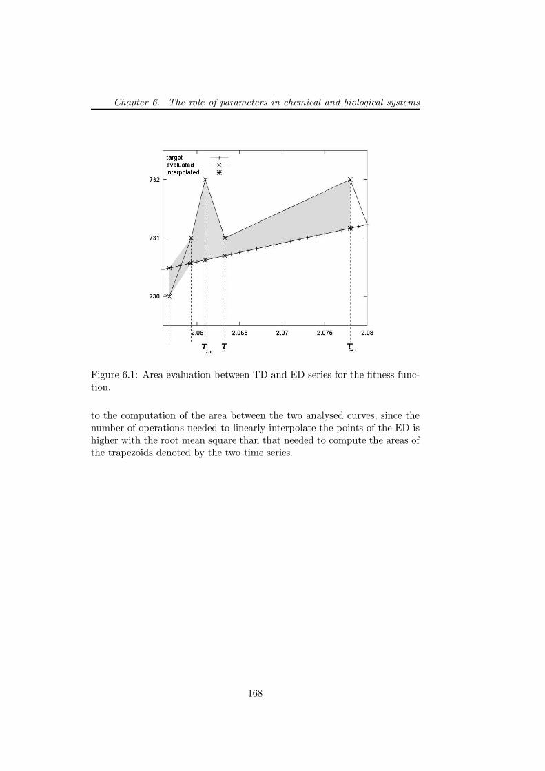
Chapter 6. The role of parameters in chemical and biological systems
Figure 6.1: Area evaluation between TD and ED series for the fitness func-tion.
to the computation of the area between the two analysed curves, since thenumber of operations needed to linearly interpolate the points of the ED ishigher with the root mean square than that needed to compute the areas ofthe trapezoids denoted by the two time series.
168
6.4. A comparison of GAs and PSO for parameter estimation in stochasticbiochemical systems
6.4 A comparison of GAs and PSO for parameterestimation in stochastic biochemical systems
Optimization methods can be used to tackle the calibration problem of pa-rameter estimation of biochemical systems by minimizing a cost function(e.g. a distance measure) which quantitatively defines how good is the sys-tem behavior using the predicted values, with respect to the experimentaldynamics. Several global optimization techniques (see [173, 137] and refer-ences therein) have already been adopted for parameter estimation of bio-chemical and biological systems. A peculiarity of our approach, with respectto other methods previously investigated for this problem, is that it embedsthe (forward) problem of performing stochastic simulations of a system dy-namics, into the inverse problem of estimating its unknown parameters. Thisleads to the development of a method that exploits the outcome of stochasticsimulation algorithms to effectively compute the fitness function value usedby the optimization techniques here investigated. In particular, we comparethe performances of genetic algorithms (GAs) and particle swarm optimiza-tion (PSO) for the parameter estimation of two simple biochemical schemeswhich are well representative of the dynamics of many other biological sys-tems: a basic catalytic kinetics (the Michaelis-Menten system), a sustainedoscillating behavior and a damped oscillating behavior (both based on theBelousov-Zhabotinskii reaction).
The choice of these two particular optimisation techniques is motivatedby the fact that parameter estimation is an example of dynamic optimiza-tion problems, meaning that the fitness function may change (more precisely,each individual can have slightly different fitness values each time it is eval-uated) and a number of contributions exist about the use of GAs and PSOfor this kind of problems (see, e.g., [115, 95]).
In the following sections we will recall some basic notions of biochemicalreactions, and describe the two simple systems (Michaelis-Menten reactionand the Brussellator) that we will consider for parameter estimation. After-wards, we describe the versions of GAs and PSO that we have used. Theexperimental results are finally presented together with further applicationsof these methods and some open problems.
6.4.1 Systems of biochemical reactions
Any generic (bio)chemical reaction can be written in the form r :∑N1
i=1 αiRi
→∑N2
j=1 βjPj , where R1, . . . , RN1are distinct reactant molecular species and
P1, . . . , PN2are distinct products, for some N1, N2 ≥ 0. The non-negative
integers αi, βj are the stoichiometric coefficients of the reaction r; they spec-ify how many molecules of each reagent species are necessary to trigger thereaction, and how many product molecules are formed after the reactionhas occurred. Each reaction is also characterized by a numerical factor,
169
Chapter 6. The role of parameters in chemical and biological systems
called the rate constant, which determines – together with the amount ofreagents – the rate, or velocity, of the reaction itself. The kinetics of a reac-tion is influenced by many factors, such as temperature, pressure, amountsof reactants, molecular crowding, etc. As a consequence, the experimentaldetermination of rate constants for a given biochemical system is not a triv-ial task, and the situation gets even harder when considering more complexbiological systems, like metabolic pathways or cellular processes in general.For further notions about biochemical reactions and chemical kinetics werefer to [39, 146].
Michaelis-Menten system. The first chemical system we consider, theMichaelis-Menten (MM) kinetics, describes the catalytic transformation ofone-reacting substrate (denoted by S) into a final product (P ) mediatedby an enzyme (E), passing through the (relatively fast) reversible forma-tion of the enzyme-substrate intermediate complex (ES). The role of Eis to lower the energy required by S for its interconversion to P ; the en-zymatic kinetics assumes that S and E are in a fast equilibrium with thecomplex they form, which then dissociates to yield the product while releas-ing the enzyme free. The set of chemical reactions corresponding to MMis: E + S
c1−→ ES,ESc2−→ E + S,ES
c3−→ E + P , where c1, c2, c3 are thestochastic constants that encompass the physical and chemical properties ofthe reaction. The initial amounts of the substrate and the enzyme used togenerate the target dynamics for our problem of parameter estimation areS = 1000, E = 750 molecules, while the stochastic constant values (that wewant to estimate with GAs and PSO) are c1 = 2.5 · 10−3, c2 = 0.1, c3 = 5.The dynamics corresponding to this set of parameters is shown in Figure6.5 (top left graph, with solid lines).
Brussellator system. The second chemical system we consider, calledBrussellator [199], is a simplified scheme for the Belousov-Zhabotinskii re-action, a family of inorganic redox reaction systems that exhibit macro-scopic temporal oscillations and spatial patterns formation. This theoreti-cal scheme is recognized as the prototype of nonlinear oscillating (open andwell-stirred) systems, proving the significance and variety of both spatialorganizations and complex rhythms occurring in many biological systems.Here, we give a description of the Brussellator that slightly differs from theoriginal one: with respect to the formulation given in [199], we leave outthe presence of two products (since they are not directly involved in theformation of the oscillating limit cycle), and we consider the following set
of reactions: Ac1−→ X,B + X
c2−→ Y, 2X + Yc3−→ 3X,X
c4−→ λ, where A,Bare two chemicals that are given as input and always kept at a constantamount, X,Y are the intermediate product chemicals that exhibit oscilla-tions, and λ represents the degradation of species X. The initial amounts
170
6.4. A comparison of GAs and PSO for parameter estimation in stochasticbiochemical systems
of molecules used for generating the target dynamics for parameter estima-tion are A = X = 200, B = 600 and Y = 300. In this case, we considertwo distinct sets of values for the reaction constants c1, c2, c3, c4 to beestimated using GAs and PSO. The set 1, 5 · 10−3, 2.5 · 10−5, 1.5 givesrise to sustained and periodic oscillations in the species X,Y , while theset 1, 5 · 10−3, 2.5 · 10−4, 1.5 gives rise to damped oscillations and quicklydrives the system dynamics to a steady-state. The corresponding dynamicsare shown (with solid and dashed lines) in Figure 6.5 (top right and bottom,respectively).
6.4.2 GAs and PSO settings
The GAs and PSO formulations used in this work evolve individuals of thesame shape: n-length vectors of floating point numbers, where n is thenumber of rate constants to optimise. That is, each allele of an individualcorresponds to one parameter that has to be estimated. The experimentalsettings and the related choices that we have done for GAs and PSO aredescribed below.
Genetic algorithms. The most commonly used GAs formulation evolvesfixed length strings over a finite alphabet, while in our case each allele cancontain any floating point value from a limited range. This GAs version isoften called real-valued or real-coded GAs (see, e.g., [204] and Section 2.1).Many sophisticated genetic operators for real-coded GAs have recently beendefined (like, for instance, Laplace Crossover, Makinen, Periaux and Toiva-nen Mutation, Non-Uniform Mutation [48]), but in this study we considerclassical operators, like the ones originally defined in [204]: one point andaverage crossover, gaussian mutation, range mutation and reinitialization.
One point crossover is similar to the standard GAs crossover definedby Holland in [89]: parents are aligned, one crossover point is selected andsubstrings are inverted to generate offspring. Average crossover returns oneoffspring that contains at each position the average values of the parentschromosomes. In this work, crossover is executed with a 0.95 rate. Incase crossover is not executed, parents are copied in the next populationwith no modification (reproduction). Otherwise, one operator among onepoint crossover and average crossover is chosen with uniform probabilitydistribution.
Gaussian mutation perturbs an allele with a number drawn from a nor-mal distribution with mean µ equal to the current value of that allele andσ = 0.05·µ. Range mutation increments or decrements an allele of a prefixedquantity (equal to 5% of its admissible range size in this work). Reinitial-ization changes the value currently contained in an allele with an uniformlydistributed random number in the admissible range. For each individual inthe spring, mutation is applied to each allele with probability 1/n, where n is
171
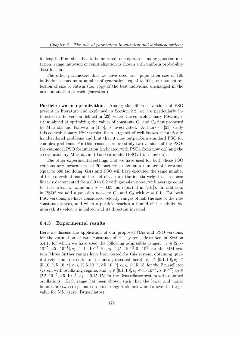
Chapter 6. The role of parameters in chemical and biological systems
its length. If an allele has to be mutated, one operator among gaussian mu-tation, range mutation or reinitialization is chosen with uniform probabilitydistribution.
The other parameters that we have used are: population size of 100individuals; maximum number of generations equal to 100; tournament se-lection of size 5; elitism (i.e. copy of the best individual unchanged in thenext population at each generation).
Particle swarm optimization. Among the different versions of PSOpresent in literature and explained in Section 2.2, we are particularly in-terested in the version defined in [23], where the co-evolutionary PSO algo-rithm aimed at optimizing the values of constants C1 and C2 first proposedby Miranda and Fonseca in [135], is investigated. Authors of [23] studythis co-evolutionary PSO version for a large set of well-known theoreticallyhand-tailored problems and hint that it may outperform standard PSO forcomplex problems. For this reason, here we study two versions of the PSO:the canonical PSO formulation (indicated with PSO1 from now on) and theco-evolutionary Miranda and Fonseca model (PSO2 from now on).
The other experimental settings that we have used for both these PSOversions are: swarm size of 20 particles; maximum number of iterationsequal to 500 (so doing, GAs and PSO will have executed the same numberof fitness evaluations at the end of a run); the inertia weight w has beenlinearly decremented from 0.9 to 0.2 with gaussian noise, with average equalto the current w value and σ = 0.05 (as reported in [201]). In addition,in PSO2 we add a gaussian noise to C1 and C2 with σ = 0.1. For bothPSO versions, we have considered velocity ranges of half the size of the rateconstants ranges, and when a particle reaches a bound of the admissibleinterval, its velocity is halved and its direction inverted.
6.4.3 Experimental results
Here we discuss the application of our proposed GAs and PSO versions,for the estimation of rate constants of the systems described in Section6.4.1, for which we have used the following admissible ranges: c1 ∈ [2.5 ·10−5, 2.5 · 10−1], c2 ∈ [1 · 10−3, 10], c3 ∈ [5 · 10−2, 5 · 102] for the MM sys-tem (three further ranges have been tested for this system, obtaining qual-itatively similar results to the ones presented here); c1 ∈ [0.1, 10], c2 ∈[5·10−4, 5·10−2], c3 ∈ [2.5·10−6, 2.5·10−4], c4 ∈ [0.15, 15] for the Brussellatorsystem with oscillating regime, and c1 ∈ [0.1, 10], c2 ∈ [5 ·10−4, 5 ·10−2], c3 ∈[2.5 ·10−5, 2.5 ·10−3], c4 ∈ [0.15, 15] for the Brussellator system with dampedoscillations. Each range has been chosen such that the lower and upperbounds are two (resp. one) orders of magnitude below and above the targetvalue for MM (resp. Brussellator).
172
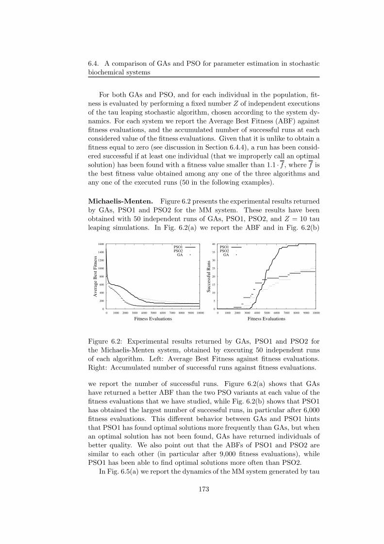
6.4. A comparison of GAs and PSO for parameter estimation in stochasticbiochemical systems
For both GAs and PSO, and for each individual in the population, fit-ness is evaluated by performing a fixed number Z of independent executionsof the tau leaping stochastic algorithm, chosen according to the system dy-namics. For each system we report the Average Best Fitness (ABF) againstfitness evaluations, and the accumulated number of successful runs at eachconsidered value of the fitness evaluations. Given that it is unlike to obtain afitness equal to zero (see discussion in Section 6.4.4), a run has been consid-ered successful if at least one individual (that we improperly call an optimalsolution) has been found with a fitness value smaller than 1.1 · f , where f isthe best fitness value obtained among any one of the three algorithms andany one of the executed runs (50 in the following examples).
Michaelis-Menten. Figure 6.2 presents the experimental results returnedby GAs, PSO1 and PSO2 for the MM system. These results have beenobtained with 50 independent runs of GAs, PSO1, PSO2, and Z = 10 tauleaping simulations. In Fig. 6.2(a) we report the ABF and in Fig. 6.2(b)
0
200
400
600
800
1000
1200
1400
1600
0 1000 2000 3000 4000 5000 6000 7000 8000 9000 10000
Av
erag
e B
est
Fit
nes
s
Fitness Evaluations
PSO1PSO2
GA
0
5
10
15
20
25
30
35
40
0 1000 2000 3000 4000 5000 6000 7000 8000 9000 10000
Su
cces
sfu
l R
un
s
Fitness Evaluations
PSO1PSO2
GA
Figure 6.2: Experimental results returned by GAs, PSO1 and PSO2 forthe Michaelis-Menten system, obtained by executing 50 independent runsof each algorithm. Left: Average Best Fitness against fitness evaluations.Right: Accumulated number of successful runs against fitness evaluations.
we report the number of successful runs. Figure 6.2(a) shows that GAshave returned a better ABF than the two PSO variants at each value of thefitness evaluations that we have studied, while Fig. 6.2(b) shows that PSO1has obtained the largest number of successful runs, in particular after 6,000fitness evaluations. This different behavior between GAs and PSO1 hintsthat PSO1 has found optimal solutions more frequently than GAs, but whenan optimal solution has not been found, GAs have returned individuals ofbetter quality. We also point out that the ABFs of PSO1 and PSO2 aresimilar to each other (in particular after 9,000 fitness evaluations), whilePSO1 has been able to find optimal solutions more often than PSO2.
In Fig. 6.5(a) we report the dynamics of the MM system generated by tau
173
Chapter 6. The role of parameters in chemical and biological systems
leaping using the constants found by the best solution generated by PSO1over the considered 50 runs, which are c1 = 0.00245, c2 = 0.02691, c3 =5.03552. We compare this dynamics (dots) with the target curves (solidlines), pointing out that it very well approximates the targets for each oneof the four chemicals involved in the reaction (E, S, ES, P ).
Brussellator with oscillating regime. Figure 6.3 reports the experi-mental results returned by GAs, PSO1 and PSO2 for the Brussellator sys-tem with oscillating regime. In particular, Fig. 6.3(a) reports the ABF and
5000
10000
15000
20000
0 1000 2000 3000 4000 5000 6000 7000 8000 9000 10000
Av
erag
e B
est
Fit
nes
s
Fitness Evaluations
PSO1PSO2
GA
0
0.2
0.4
0.6
0.8
1
0 1000 2000 3000 4000 5000 6000 7000 8000 9000 10000
Su
cces
sfu
l R
un
s
Fitness Evaluations
PSO1PSO2
GA
Figure 6.3: Experimental results returned by GAs, PSO1 and PSO2 forthe Brussellator system with oscillating regime, obtained by executing 50independent runs of each algorithm. Left: Average Best Fitness againstfitness evaluations. Right: Accumulated number of successful runs againstfitness evaluations.
Fig. 6.3(b) reports the number of successful runs. These results have beenobtained with 50 independent runs of GAs, PSO1, PSO2; in this case, onlyone tau leaping execution (Z = 1) has been performed because, if we executemore than one run and we calculate their average behaviours, we would riskto flatten the oscillations that characterize this dynamics.
In this case, it is clear that PSO outperforms GAs both from the ABFand success rate viewpoints. In particular, we point out that neither GAsnor PSO2 have been able to find an optimal solution in none of the 50independent executions that we have performed, while PSO1 has found anoptimal solution in only a single run after a number of fitness evaluationsapproximately equal to 3,500. We conclude that PSO1 can be consideredthe most suitable algorithm, among the ones that we have studied, for thisparticular Brussellator dynamics.
Figure 6.5(b) reports the dynamics (dots) over one period of the Brus-sellator system with oscillating regime that we have obtained using the con-stants found by the best solution generated by PSO1 over the 50 runs thatwe have executed. We also observe that the target behavior (lines) has
174
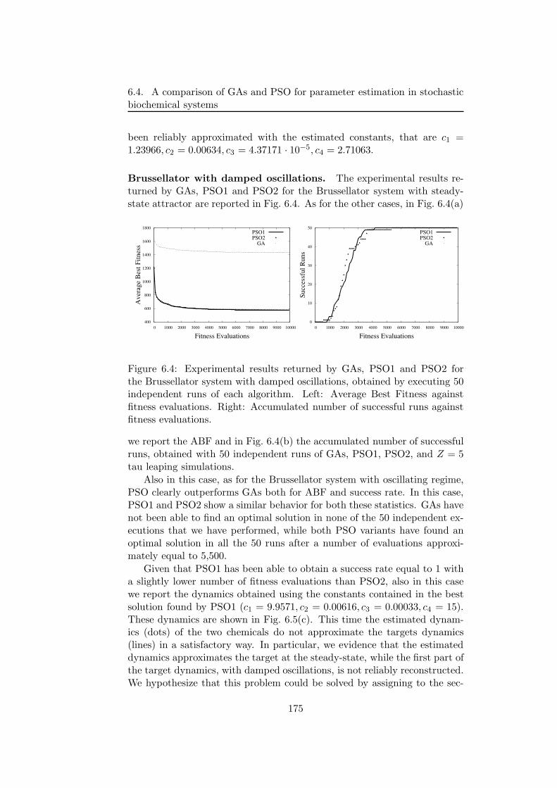
6.4. A comparison of GAs and PSO for parameter estimation in stochasticbiochemical systems
been reliably approximated with the estimated constants, that are c1 =1.23966, c2 = 0.00634, c3 = 4.37171 · 10−5, c4 = 2.71063.
Brussellator with damped oscillations. The experimental results re-turned by GAs, PSO1 and PSO2 for the Brussellator system with steady-state attractor are reported in Fig. 6.4. As for the other cases, in Fig. 6.4(a)
400
600
800
1000
1200
1400
1600
1800
0 1000 2000 3000 4000 5000 6000 7000 8000 9000 10000
Av
erag
e B
est
Fit
nes
s
Fitness Evaluations
PSO1PSO2
GA
0
10
20
30
40
50
0 1000 2000 3000 4000 5000 6000 7000 8000 9000 10000
Su
cces
sfu
l R
un
s
Fitness Evaluations
PSO1PSO2
GA
Figure 6.4: Experimental results returned by GAs, PSO1 and PSO2 forthe Brussellator system with damped oscillations, obtained by executing 50independent runs of each algorithm. Left: Average Best Fitness againstfitness evaluations. Right: Accumulated number of successful runs againstfitness evaluations.
we report the ABF and in Fig. 6.4(b) the accumulated number of successfulruns, obtained with 50 independent runs of GAs, PSO1, PSO2, and Z = 5tau leaping simulations.
Also in this case, as for the Brussellator system with oscillating regime,PSO clearly outperforms GAs both for ABF and success rate. In this case,PSO1 and PSO2 show a similar behavior for both these statistics. GAs havenot been able to find an optimal solution in none of the 50 independent ex-ecutions that we have performed, while both PSO variants have found anoptimal solution in all the 50 runs after a number of evaluations approxi-mately equal to 5,500.
Given that PSO1 has been able to obtain a success rate equal to 1 witha slightly lower number of fitness evaluations than PSO2, also in this casewe report the dynamics obtained using the constants contained in the bestsolution found by PSO1 (c1 = 9.9571, c2 = 0.00616, c3 = 0.00033, c4 = 15).These dynamics are shown in Fig. 6.5(c). This time the estimated dynam-ics (dots) of the two chemicals do not approximate the targets dynamics(lines) in a satisfactory way. In particular, we evidence that the estimateddynamics approximates the target at the steady-state, while the first part ofthe target dynamics, with damped oscillations, is not reliably reconstructed.We hypothesize that this problem could be solved by assigning to the sec-
175

Chapter 6. The role of parameters in chemical and biological systems
0
200
400
600
800
1000
0 0.5 1 1.5 2 2.5 3
Mo
lecu
les
Time [a.u.]
E
ES
P
S
0
500
1000
1500
2000
2500
0 5 10 15 20 25
Mo
lecu
les
Time [a.u.]
XY
X targetY target
50
100
150
200
250
300
350
400
0 5 10 15 20 25
Mo
lecu
les
Time [a.u.]
XY
X targetY target
Figure 6.5: Dynamics of the studied systems using the constants found bythe best solution generated by PSO1. Left: Michaelis-Menten system; Right:Brussellator with oscillating regime; Bottom: Brussellator with damped os-cillations.
ond (non-oscillatory) part of the dynamics a lower weight than to the first(oscillatory) one in the fitness calculation.
6.4.4 Discussion
The problem of estimating the rate constants of two well known biochem-ical systems has been tackled in this section, using GAs and two differentversions of PSO. The experimental results that we have obtained hint thatcanonical PSO is a suitable optimization method for this problem, since itoutperforms both GAs and the PSO version that co-evolves parameters C1
and C2. The values of the constants returned by PSO have allowed us tofaithfully reconstruct the behavior of the MM system and of the oscillat-ing Brussellator. Nevertheless, for the damped Brussellator even the bestset of constants found by PSO has not allowed us to reconstruct the targetdynamics in a suitable way. Thus, even though interesting, the presentedresults deserve further investigations.
Some possible improvements to the proposed optimization methods in-clude the use of further GAs genetic operators, for instance, Laplace Cross-
176
6.4. A comparison of GAs and PSO for parameter estimation in stochasticbiochemical systems
over, Makinen, Periaux and Toivanen Mutation, Non-Uniform Mutation [48]and the other operators described in Section 2.1, or other PSO models,like PSO with structured populations, with various different neighbourhoodstructures or with more than two basins of attraction (in addition to thelocal and global best positions).
Another possible improvement concerns the fitness function. The defini-tion of a suitable fitness function is an intrinsically difficult task for param-eter estimation of biochemical systems, for several reasons. First of all, ifwe exploit stochastic simulation algorithms for the fitness calculation, thenit is very unlike to reach the (ideal) value of zero because of the stochasticfluctuations of the estimated time series. Moreover, the same individualwill generally have different fitness values each time it is evaluated. Thesedrawbacks could be mitigated by, for instance, executing many times thetau leaping algorithm and calculating averages, but this might be very timeconsuming in some cases and it could raise serious problems when the targetdynamics shows an oscillating behavior (averages may flatten oscillations).
In addition, regarding the fitness function, our choice of using tau leapingto generate the dynamics corresponding to a given set of constants (and thusto evaluate the fitness of an individual) has suggested us to consider the areabetween the target and the estimated curves, instead of calculating theirpoint-to-point mutual distance. In fact, since the tau leaping algorithmsamples points at arbitrary time instants, we have to deal with irregulartiming patterns; furthermore, some portions of the dynamics might be morefrequently sampled than others. If we use the point-to-point distance tocalculate fitness, all sampled points would receive the same importance, thusoverrating the dynamics portions that have been more frequently sampled.On the other hand, the area calculation allows us to better evaluate thedynamics also in regions that have not been sampled by tau leaping, andthus approximate more faithfully the (ideal) situation in which we haveinformation for each possible time instant.
To try and solve these problems, this fitness definition could be fur-ther improved, for instance, in two ways. The first consists in partitioningthe time axis into subintervals, and performing the optimization by incre-mentally extending the time interval considered for the fitness calculation.The second consists in giving different weights to regions of the dynam-ics that show distinct behaviours, according to some previous knowledge ofthe system. Moreover, a different weight could be assigned to the variousspecies involved in the chemical reactions under consideration according, forinstance, to the relevance they hold within the system.
Finally, we have recently applied the PSO versions presented here for theparameter estimation of the chemotaxis model described in Section 5.4.1; thepreliminary, but promising results of this work can be found in [13].
177
Chapter 6. The role of parameters in chemical and biological systems
6.5 Stochastic simulations on a grid frameworkfor parameter sweep applications in biological
models
In this section we present the distribution of a large number of computationsof τ -DPP stochastic simulator (see [30] and Chapter 4 for additional details),on the EGEE grid framework [56], to enable an analysis of the parameterspace of a biochemical system by means of parameter sweep applications(PSAs) [140]. This is done to the aim of exploring this high–dimensional re-search space, and gain knowledge about the influence of the initial conditionson the system’s dynamics.
Given the biological model to analyse, the first step is to define the rangesand the distribution of the parameters values that will be perturbed duringthe PSA. The most intuitive way to define a set of parametrisations involvesthe cartesian product of the admissible ranges of each parameter; however,since we have to deal with a high number of parameters, the number ofdifferent parametrisation needed to cover the entire research space wouldbe troublesome. A more efficient method to sample this multidimensionalspace exploits the quasi-random series [149], also called low discrepancysequences. The discrepancy of a sequence is a measure of its uniformity, andis computed by comparing the actual number of sample points in a givenmultidimensional space with the number of sample points that “should be”there assuming a uniform distribution. Therefore, the aim of quasi-randomseries is to “uniformely” cover the space with “few” samples (i.e., with alower number of points with respect to classic uniform distributions).
Since each instance of a PSA – corresponding to a simulation of thebiochemical system by means of τ -DPP –2 is independent, the grid comput-ing framework constitutes a good solution to tackle the high computationalcost of this kind of application. The advantage of using a grid distributedapproach for computing large computational challenges relies on the high-end scalability of this technology. If jobs are completely independent thetheoretical scalability of the system is linear. This is not true in real com-putations, due to the time needed to schedule jobs, to transfer data and toresubmit failed jobs. However, while distributed platform are not suitableto parallelise the execution of programs that require high connectivity, theyare very reliable for data parallel applications, by splitting the computationof input data in independent processes and collecting back the results.
As a case study, we present a PSA for the exploration of the stochasticconstants values space of a model composed by 59 reactions which describesthe bacterial chemotaxis process presented in Section 5.4.1. This approachrepresents a benchmark for the development of a sensitivity analysis tool forstochastic biochemical systems implemented on the grid framework.
178
6.5. Stochastic simulations on a grid frameworkfor parameter sweep applications in biological models
6.5.1 The EGEE grid platform
In this work we exploit the EGEE project infrastructure, a wide area gridplatform for scientific applications, composed of thousands of CPUs, whichimplements the Virtual Organisation (VO) paradigm [63]. The produc-tion framework is a large multi-science grid infrastructure, federating 250resource centres world-wide, which provides comprehensively 20.000 CPUsand several Petabytes of storage. This infrastructure is used on a daily basisby thousands of scientists federated in over 200 VOs.
The EGEE platform relies on the gLite middleware [103] used in severalprojects like: DataGrid, DataTag, Globus, GriPhyN, and LCG. The gLitedistribution is an integrated set of components designed to enable resourcesharing and must be installed on a local server, the User Interface (UI), toallow users to manage the EGEE grid computations. In particular, employ-ing gLite, it is possible to submit jobs to the grid, to monitor their stateof advancement, and to retrieve the outputs when the computations have anormal termination or to resubmit the job in case of failure. This grid infras-tructure is highly scalable and allows computational intensive challenges tobe accomplished, but users must cope with the continuous dynamic reshapeof the available resources, which is typical of loosely coupled distributedplatforms.
The grid middleware offers a well-established security system, which en-ables a secure connection to remote resources. This system relies on theGrid Security Infrastructure (GSI) which uses public key cryptography torecognise users. The access to remote clusters is granted by a Personal Cer-tificate, encoded in the X.509 format, associated to each job with the aim toauthenticate the user. Moreover, users must be authorised to submit jobs bya VO, that is, a grid community having similar tasks, which grants for them.In this test we join the Biomed VO, which shares on average 2000 CPUsand admits applications in the medical image processing, bioinformatics,and more generally the biomedical data processing fields.
The resources available on the EGEE project platform are composed bya network of several Computing Elements (CEs), which are gateways forcomputer clusters where jobs are actually performed, and an equal numberof Storage Elements (SEs), that implement a distributed filesystem to storetemporary files. The computational resources are connected to a ResourceBroker (RB) that routes each job on a specific CE taking into account thedirectives of the submitting script, called JDL (Job Description Language).In detail, the Workload Management System is the RB service which sched-ules jobs by delivering them to the best matching resource, balancing thecomputational load, via a Condor-G client [24]. Although this brokering isnot configurable by users, it provides high performance: bulk submissionallows to submit sets of independent jobs in a much more reliable and com-pound operation, up to a rate of 50Hz for job submission and 0.5Hz for job
179
Chapter 6. The role of parameters in chemical and biological systems
dispatching to the CEs.
Each CE submits the incoming job to a batch system queue (PBS orLFS) which hides the farm of Working Nodes. To handle files over the grid,the gLite middleware provides a set of tools to manage data similarly toa distributed filesystem. These tools allow the data to be replicated intodifferent SEs, which can help to reduce the database upload time duringthe computations. The RB, in fact, is able to redirect the execution of anapplication to a CE located as near as possible to the files currently used,hence minimising the communication time. Although large files should bealways managed by using the SEs, for both input and output, it is possible touse the SandBox to load and download small files directly to the CE. Themain difference is that files transferred using the InputSandBox and theOutputSandBox are temporary stored on the RBs, therefore are manageddirectly by the middleware (but their size should be less than few MB,otherwise RBs will be rapidly stuck) and cannot be reused. On the contrary,files on the SEs have no limitation in size and availability, but have to behandled directly by users.
6.5.2 PSA over the grid
From the computational point of view, the greatest problem of implementinga PSA over the grid is the dynamic behaviour of the available resources. Dueto network and system errors, or in relation to the global computational load,the available resources are continuously reshaped and the rate of failure incomputations is quite high.
Some solutions, such as Nimrod [22] and APST [28], have been devel-oped to handle these PSAs on grid but they rely on particular middlewareimplementations, which are not gLite compliant. Moreover, a grid-inspiredsolution to distribute stochastic simulations is described in [108], but theapproach does not rely on a grid implementation. While the infrastructureused for the PSAs presented in the following sections is a standard pro-duction environment, our focus is not on the middleware implementation,but on testing the reliability of the proposed simulation approach over thisdistributed platform, by choosing the best strategy to cope with the gridensemble. Therefore, a crucial point is the creation of a system able to in-teract with the grid to manage the whole PSA computation, which shouldcheck the consistency of each job in a fault tolerant environment.
Managing jobs over the grid: the Challenge Control System. Inthe context of the EGEE grid, the Challenge Control System (CCS) [130]was developed to completely coordinate a computational challenge runningon a single UI, by submitting and managing the whole set of jobs in whichthe computation is split dealing with CEs and SEs. In other words, thisframework provides an automatic management of all the necessary opera-
180
6.5. Stochastic simulations on a grid frameworkfor parameter sweep applications in biological models
tions to fulfil each single task, because it wraps the grid middleware low levelAPI for file handing (lcg-* ) and for job submission, status monitoring andoutput retrieving (glite-* ), by providing a user-friendly and fault-tolerantenvironment.
The CCS is highly customisable, thanks to its double layered infras-tructure: the first layer was developed to cope with the latest middlewareversions of the EGEE infrastructure to manage each single job, while thesecond level deals with the different requirements of the current applicationto split the computation and perform the specific tasks on the remote re-sources. These layers are interconnected by a MySQL database designed tocollect all the information needed to manage each grid job, which works asback-end of the system.
The first layer of the CCS works in close connection with the UI and itis mainly devoted to the management of each single job, from the definitionof the JDL script and its submission, to the retrieving of the output results.This layer employs the network time protocol using the same servers of theEGEE infrastructure, in order to be synchronised with respect to all the gridcomponents, which is crucial for enabling a correct survey on computationaltrends. Our system also makes use of the crond daemon which beats theinterval between each round of Challenge Coordination System execution inwhich, according to the information stored in the MySQL database, taskssuch as the submission of new jobs, polling the RB about the status ofscheduled jobs, the resubmission of failed jobs and the retrieve back of outputresults are accomplished.
The second layer is the most important from the application point ofview because it coordinates, by using a set of scripts, the job distributionover the grid by splitting the input data in specific tasks: their computationon remote resources and the collection of the output results. Moreover, thesecond layer checks the output consistence of each simulations computed onthe grid platform in connection with the upper layer, which monitors eachjob as an independent unit.
Implementations to distribute the PSA over the grid. A crucialfactor in the implementation of a grid application is the identification of asuitable strategy for splitting the computation into a set of grid jobs, whichcorresponds to the granularity of the computation. In fact, the computationof long jobs on the grid may cause significant data loss in case of systemfailure or problems during the data transfer. On the other hand, the exe-cution of a large number of short jobs raises the total latency time in thebatch queues, affecting the global performance of the system. Moreover,the size of the output results should be considered, due to the impact ofthe transfer time on the total computation efficiency. For this reason weperformed different PSAs, by varying the number of jobs and the number of
181
Chapter 6. The role of parameters in chemical and biological systems
simulations performed in each job, and by altering the computation time byusing different strategies of parameters selection, which consequently affectthe output size.
In order to enable the execution of a large number of τ -DPP simulationsover the grid platform, the CCS [130] has been adapted to satisfy the appli-cation requirements. While the lower layer has been periodically updatedto be compliant with the latest release of the EGEE grid middleware, theupper layer has been customised for this specific application. In detail, twoscripts of the developed framework have been modified to manage the inputand output of the PSA computation: one concerns the input managementand the other coordinates the computation on the remote resource.
The first script splits of the computation in grid jobs according to thedesired granularity. This script populates a directory in which all the files foreach single job are temporary collected for submission (i.e., the τ -DPP pro-gram and a folder tree containing the input files for each single simulation)and creates the JDL script which describes the job. It then calls the lowerlayer for the real submission to the grid, specifying some important param-eters such as the maximum number of resubmission in case of failure (whichallows to overcome most of the problems due to the dynamic reshape of thegrid facilities), the maximum time for the job to be queued on a grid clusterbefore its deletion and resubmission (to avoid over-crowded computationalresources), and the output directory on the local server where results willbe collected.
The second script of the CCS that has to be customised, is the one ef-fectively executed on the remote clusters. This script manages the inputfiles: it unpacks the input from the InputSandBox, defines the pipeline ofoperations to be accomplished on the remote resources (in this case, it iter-ates the execution of τ -DPP according to the specified granularity), rebuildsthe output directory in a structure which allows an easy evaluation of theresults, packs the results to be retrieved and transfers the output results.
The output of a PSA is constituted by a set of calculated dynamics. Inthis case, the SEs must be used to archive the numerical results before down-loading them to the UI. This approach is essential when there is the need ofretrieving the complete numerical results for a complete investigation of thesystem dynamics. However, preliminary analysis of the grid performancesuggested that the output data size have a significant effect on the overheadand the success rate of the grid infrastructure.
In order to test the grid infrastructure in a wider range of conditions, wedeveloped another approach in which the analysis of the dynamics is donejust after the simulations. In this case, the output is reduced significantly:instead of the complete time series for each molecular species, a value rep-resenting an interesting property of the considered dynamics is retrievedimmediately through the OutputSandBox, without using the SEs. In otherwords, we developed two different implementations: the first one (imple-
182
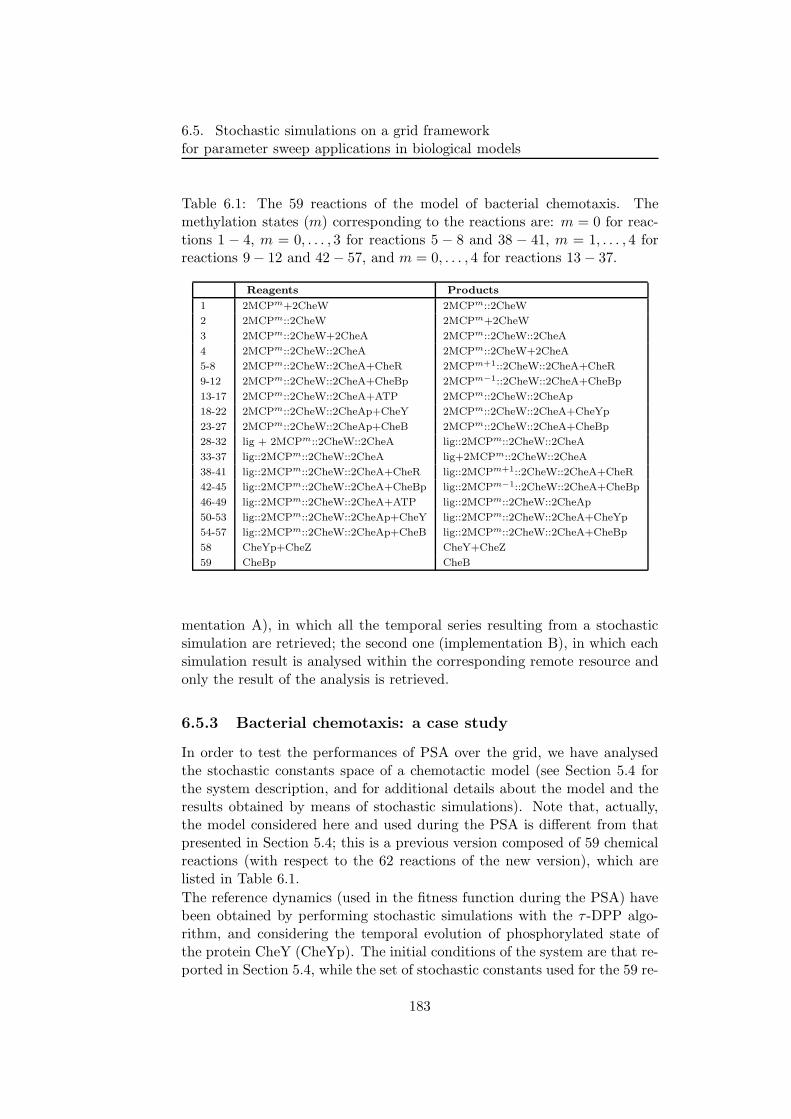
6.5. Stochastic simulations on a grid frameworkfor parameter sweep applications in biological models
Table 6.1: The 59 reactions of the model of bacterial chemotaxis. Themethylation states (m) corresponding to the reactions are: m = 0 for reac-tions 1 − 4, m = 0, . . . , 3 for reactions 5 − 8 and 38 − 41, m = 1, . . . , 4 forreactions 9 − 12 and 42 − 57, and m = 0, . . . , 4 for reactions 13 − 37.
Reagents Products
1 2MCPm+2CheW 2MCPm::2CheW
2 2MCPm::2CheW 2MCPm+2CheW
3 2MCPm::2CheW+2CheA 2MCPm::2CheW::2CheA
4 2MCPm::2CheW::2CheA 2MCPm::2CheW+2CheA
5-8 2MCPm::2CheW::2CheA+CheR 2MCPm+1::2CheW::2CheA+CheR
9-12 2MCPm::2CheW::2CheA+CheBp 2MCPm−1::2CheW::2CheA+CheBp
13-17 2MCPm::2CheW::2CheA+ATP 2MCPm::2CheW::2CheAp
18-22 2MCPm::2CheW::2CheAp+CheY 2MCPm::2CheW::2CheA+CheYp
23-27 2MCPm::2CheW::2CheAp+CheB 2MCPm::2CheW::2CheA+CheBp
28-32 lig + 2MCPm::2CheW::2CheA lig::2MCPm::2CheW::2CheA
33-37 lig::2MCPm::2CheW::2CheA lig+2MCPm::2CheW::2CheA
38-41 lig::2MCPm::2CheW::2CheA+CheR lig::2MCPm+1::2CheW::2CheA+CheR
42-45 lig::2MCPm::2CheW::2CheA+CheBp lig::2MCPm−1::2CheW::2CheA+CheBp
46-49 lig::2MCPm::2CheW::2CheA+ATP lig::2MCPm::2CheW::2CheAp
50-53 lig::2MCPm::2CheW::2CheAp+CheY lig::2MCPm::2CheW::2CheA+CheYp
54-57 lig::2MCPm::2CheW::2CheAp+CheB lig::2MCPm::2CheW::2CheA+CheBp
58 CheYp+CheZ CheY+CheZ
59 CheBp CheB
mentation A), in which all the temporal series resulting from a stochasticsimulation are retrieved; the second one (implementation B), in which eachsimulation result is analysed within the corresponding remote resource andonly the result of the analysis is retrieved.
6.5.3 Bacterial chemotaxis: a case study
In order to test the performances of PSA over the grid, we have analysedthe stochastic constants space of a chemotactic model (see Section 5.4 forthe system description, and for additional details about the model and theresults obtained by means of stochastic simulations). Note that, actually,the model considered here and used during the PSA is different from thatpresented in Section 5.4; this is a previous version composed of 59 chemicalreactions (with respect to the 62 reactions of the new version), which arelisted in Table 6.1.
The reference dynamics (used in the fitness function during the PSA) havebeen obtained by performing stochastic simulations with the τ -DPP algo-rithm, and considering the temporal evolution of phosphorylated state ofthe protein CheY (CheYp). The initial conditions of the system are that re-ported in Section 5.4, while the set of stochastic constants used for the 59 re-
183
Chapter 6. The role of parameters in chemical and biological systems
actions is: c = (c1 = 0.1, c2 = 0.01, c3 = 0.1, c4 = 0.02, c5 = 5.0·10−7, c6 =5.0 · 10−4, c7 = 2.0 · 10−4, c8 = 0.0080, c9 = 1.0, c10 = 0.6, c11 =15.0, c12 = 0.35, c13 = 5.0 · 10−7, c14 = 5.0 · 10−4, c15 = 2.0 · 10−4, c16 =6.0 · 10−4, c17 = 0.325, c18 = 7.0 · 10−6, c19 = 0.0035, c20 = 0.0014, c21 =0.0044, c22 = 0.8, c23 = 15.0, c24 = 0.325, c25 = 7.0 · 10−6, c26 =0.0035, c27 = 0.0014, c28 = 0.0044, c29 = 0.29, c30 = 2.8 · 10−5, c31 =0.014, c32 = 0.0056, c33 = 0.0175, c34 = 1.0, c35 = 15.0, c36 = 0.29, c37 =2.8 · 10−5, c38 = 0.014, c39 = 0.0056, c40 = 0.0175, c41 = 0.165, c42 =5.0·10−5, c43 = 0.025, c44 = 0.01, c45 = 0.0306, c46 = 1.2, c47 = 15.0, c48 =0.165, c49 = 5.0 · 10−5, c50 = 0.03, c51 = 0.0112, c52 = 0.0343, c53 =0.05, c54 = 6.8 · 10−5, c55 = 0.0336, c56 = 0.0135, c57 = 0.035, c58 =1.4, c59 = 15.0).
6.5.4 Results
For each specific PSA we decided to perform in every single job a constantnumber of simulations of the system, in order to keep constant the expectedCPU time, tcpu
e , for each job within every single PSA. However, the numberof simulations and jobs is different in each PSA, according to the purposeof each test and to test the grid using different settings. Therefore, PSAsdiffer with each other for what concerns the number of simulations groupedin each job and for the number of grid jobs, which have comprehensively atcpue between 0.5 and 3.5 hours. Jobs within this interval are defined long
jobs, in opposition to medium jobs (between 5 and 45 minutes) and short jobs(less than 5 minutes). Long jobs are largely considered the most suitableto exploit grid computing because they represent a good trade-off betweenlatency and failure problems [69]. Therefore, the proposed job durationinterval is appropriate to value the efficiency of grid in this PSAs challenge.
Four PSAs, in the following called PSA1, PSA2, PSA3 and PSA4, havebeen performed on the bacterial chemotaxis model described in Section 6.5.3.The parametrisations of each PSA have been defined by perturbing one ormore values of the set c = (c1, . . . , c59) of stochastic constants of the model,with respect to the values in c (used to obtain the target dynamics).
The results of the stochastic simulations performed on the grid have beenanalysed by comparing them to the target dynamics, exploiting the fitnessfunction described in Section 6.3.
PSA1 and PSA2. In PSA1 and PSA2, only one element of the stochasticconstants vector c has been perturbed in each parametrisation. In PSA1,for each parameter cj ∈ c, 10 simulations have been run using 10 values ofcj linearly distributed within the interval [0.5 · cj , 1.5 · cj], where cj is thereference value of each constant cj, j = 1, . . . , 59. A total of 590 simulationshave been distributed over the grid, organised in jobs of 10 simulations each.Every simulation has been initialised with a relative long time length, 10 time
184
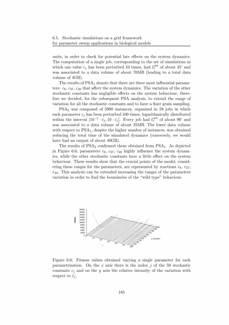
6.5. Stochastic simulations on a grid frameworkfor parameter sweep applications in biological models
units, in order to check for potential late effects on the system dynamics.The computation of a single job, corresponding to the set of simulations inwhich one value cj has been perturbed 10 times, had tcpu
e of about 45’ andwas associated to a data volume of about 70MB (leading to a total datavolume of 4GB).
The results of PSA1 denote that there are three most influential parame-ters: c8, c37, c49 that affect the system dynamics. The variation of the otherstochastic constants has negligible effects on the system behaviour, there-fore we decided, for the subsequent PSA analysis, to extend the range ofvariation for all the stochastic constants and to have a finer grain sampling.
PSA2 was composed of 5900 instances, organised in 59 jobs in whicheach parameter cj has been perturbed 100 times, logarithmically distributedwithin the interval [10−1 · cj , 10 · cj]. Every job had tcpu
e of about 90’ andwas associated to a data volume of about 25MB. The lower data volumewith respect to PSA1, despite the higher number of instances, was obtainedreducing the total time of the simulated dynamics (conversely, we wouldhave had an output of about 40GB).
The results of PSA2 confirmed those obtained from PSA1. As depictedin Figure 6.6, parameters c8, c37, c49 highly influence the system dynam-ics, while the other stochastic constants have a little effect on the systembehaviour. These results show that the crucial points of the model, consid-ering these ranges for the parameters, are represented by reactions r8, r37,r49. This analysis can be extended increasing the ranges of the parametersvariation in order to find the boundaries of the “wild type” behaviour.
0 10
20 30
40 50
60 0 10
20 30
40 50
60 70
80 90
100
0 2000 4000 6000 8000
10000 12000 14000 16000 18000 20000
fitne
ss
j
cj variation
fitne
ss
Figure 6.6: Fitness values obtained varying a single parameter for eachparametrisation. On the x axis there is the index j of the 59 stochasticconstants cj and on the y axis the relative intensity of the variation withrespect to cj .
185
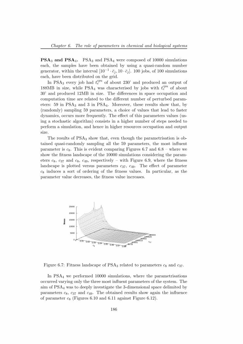
Chapter 6. The role of parameters in chemical and biological systems
PSA3 and PSA4. PSA3 and PSA4 were composed of 10000 simulationseach, the samples have been obtained by using a quasi-random numbergenerator, within the interval [10−1 · cj, 10 · cj ]. 100 jobs, of 100 simulationseach, have been distributed on the grid.
In PSA3 every job had tcpue of about 230’ and produced an output of
188MB in size, while PSA4 was characterised by jobs with tcpue of about
30’ and produced 12MB in size. The differences in space occupation andcomputation time are related to the different number of perturbed param-eters: 59 in PSA3 and 3 in PSA4. Moreover, these results show that, by(randomly) sampling 59 parameters, a choice of values that lead to fasterdynamics, occurs more frequently. The effect of this parameters values (us-ing a stochastic algorithm) consists in a higher number of steps needed toperform a simulation, and hence in higher resources occupation and outputsize.
The results of PSA3 show that, even though the parametrisation is ob-tained quasi-randomly sampling all the 59 parameters, the most influentparameter is c8. This is evident comparing Figures 6.7 and 6.8 – where weshow the fitness landscape of the 10000 simulations considering the param-eters c8, c37 and c8, c49, respectively – with Figure 6.9, where the fitnesslandscape is plotted versus parameters c37, c49. The effect of parameterc8 induces a sort of ordering of the fitness values. In particular, as theparameter value decreases, the fitness value increases.
0 0.01 0.02 0.03 0.04 0.05 0.06 0.07 0.08 0 5e-05
0.0001 0.00015
0.0002 0.00025
0.0003
0
5000
10000
15000
20000
25000
fitne
ss
c8
c37
fitne
ss
Figure 6.7: Fitness landscape of PSA3 related to parameters c8 and c37.
In PSA4 we performed 10000 simulations, where the parametrisationsoccurred varying only the three most influent parameters of the system. Theaim of PSA4 was to deeply investigate the 3-dimensional space delimited byparameters c8, c37 and c49. The obtained results show again the influenceof parameter c8 (Figures 6.10 and 6.11 against Figure 6.12).
186
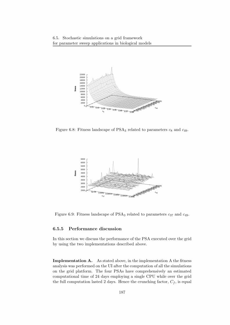
6.5. Stochastic simulations on a grid frameworkfor parameter sweep applications in biological models
0 0.01 0.02 0.03 0.04 0.05 0.06 0.07 0.08 0 5e-05 0.0001 0.00015 0.0002 0.00025 0.0003 0.00035 0.0004 0.00045 0.0005
0
2000
4000
6000
8000
10000
12000
14000
16000
18000
20000
22000fit
ness
c8
c49
fitne
ss
Figure 6.8: Fitness landscape of PSA3 related to parameters c8 and c49.
0 5e-05 0.0001 0.00015 0.0002 0.00025 0.0003 0 5e-05 0.0001 0.00015 0.0002 0.00025 0.0003 0.00035 0.0004 0.00045 0.0005
2000
2500
3000
3500
4000
4500
5000
5500
6000
6500
fitne
ss
c37
c49
fitne
ss
Figure 6.9: Fitness landscape of PSA3 related to parameters c37 and c49.
6.5.5 Performance discussion
In this section we discuss the performance of the PSA executed over the gridby using the two implementations described above.
Implementation A. As stated above, in the implementation A the fitnessanalysis was performed on the UI after the computation of all the simulationson the grid platform. The four PSAs have comprehensively an estimatedcomputational time of 24 days employing a single CPU while over the gridthe full computation lasted 2 days. Hence the crunching factor, Cf , is equal
187
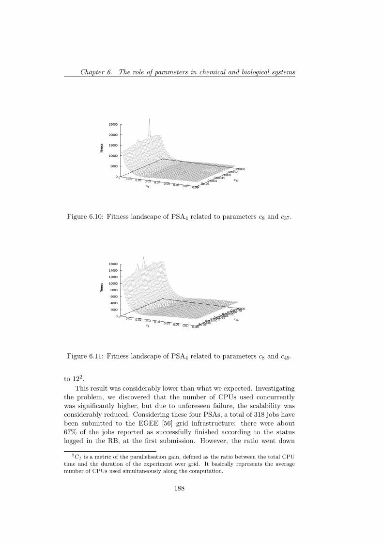
Chapter 6. The role of parameters in chemical and biological systems
0 0.01 0.02 0.03 0.04 0.05 0.06 0.07 0.08 0 5e-05
0.0001 0.00015
0.0002 0.00025
0.0003
0
5000
10000
15000
20000
25000
fitne
ss
c8
c37
fitne
ss
Figure 6.10: Fitness landscape of PSA4 related to parameters c8 and c37.
0 0.01 0.02 0.03 0.04 0.05 0.06 0.07 0.08 0 5e-05 0.0001 0.00015 0.0002 0.00025 0.0003 0.00035 0.0004 0.00045 0.0005
0
2000
4000
6000
8000
10000
12000
14000
16000
fitne
ss
c8
c49
fitne
ss
Figure 6.11: Fitness landscape of PSA4 related to parameters c8 and c49.
to 122.
This result was considerably lower than what we expected. Investigatingthe problem, we discovered that the number of CPUs used concurrentlywas significantly higher, but due to unforeseen failure, the scalability wasconsiderably reduced. Considering these four PSAs, a total of 318 jobs havebeen submitted to the EGEE [56] grid infrastructure: there were about67% of the jobs reported as successfully finished according to the statuslogged in the RB, at the first submission. However, the ratio went down
2Cf is a metric of the parallelisation gain, defined as the ratio between the total CPU
time and the duration of the experiment over grid. It basically represents the averagenumber of CPUs used simultaneously along the computation.
188
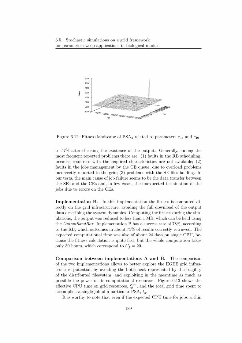
6.5. Stochastic simulations on a grid frameworkfor parameter sweep applications in biological models
0 5e-05 0.0001 0.00015 0.0002 0.00025 0.0003 0 5e-05 0.0001 0.00015 0.0002 0.00025 0.0003 0.00035 0.0004 0.00045 0.0005
1000
2000
3000
4000
5000
6000
7000
8000fit
ness
c37
c49
fitne
ss
Figure 6.12: Fitness landscape of PSA4 related to parameters c37 and c49.
to 57% after checking the existence of the output. Generally, among themost frequent reported problems there are: (1) faults in the RB scheduling,because resources with the required characteristics are not available; (2)faults in the jobs management by the CE queue, due to overload problemsincorrectly reported to the grid; (3) problems with the SE files holding. Inour tests, the main cause of job failure seems to be the data transfer betweenthe SEs and the CEs and, in few cases, the unexpected termination of thejobs due to errors on the CEs.
Implementation B. In this implementation the fitness is computed di-rectly on the grid infrastructure, avoiding the full download of the outputdata describing the system dynamics. Computing the fitness during the sim-ulations, the output was reduced to less than 1 MB, which can be held usingthe OutputSandBox. Implementation B has a success rate of 78%, accordingto the RB, which outcomes in about 75% of results correctly retrieved. Theexpected computational time was also of about 24 days on single CPU, be-cause the fitness calculation is quite fast, but the whole computation takesonly 30 hours, which correspond to Cf = 20.
Comparison between implementations A and B. The comparisonof the two implementations allows to better explore the EGEE grid infras-tructure potential, by avoiding the bottleneck represented by the fragilityof the distributed filesystem, and exploiting in the meantime as much aspossible the power of its computational resources. Figure 6.13 shows theeffective CPU time on grid resources, tcpu
g , and the total grid time spent toaccomplish a single job of a particular PSA, tg.
It is worthy to note that even if the expected CPU time for jobs within
189
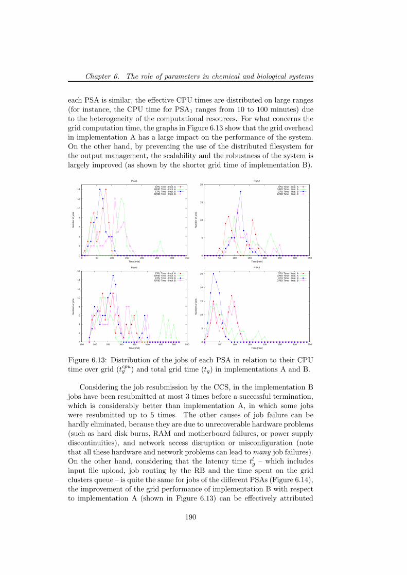
Chapter 6. The role of parameters in chemical and biological systems
each PSA is similar, the effective CPU times are distributed on large ranges(for instance, the CPU time for PSA1 ranges from 10 to 100 minutes) dueto the heterogeneity of the computational resources. For what concerns thegrid computation time, the graphs in Figure 6.13 show that the grid overheadin implementation A has a large impact on the performance of the system.On the other hand, by preventing the use of the distributed filesystem forthe output management, the scalability and the robustness of the system islargely improved (as shown by the shorter grid time of implementation B).
0
2
4
6
8
10
12
14
0 50 100 150 200 250 300 350
Num
ber
of jo
bs
Time [min]
PSA1
CPU Time - Impl. AGRID Time - Impl. ACPU Time - Impl. B
GRID Time - Impl. B
0
5
10
15
20
0 50 100 150 200 250 300 350
Num
ber
of jo
bs
Time [min]
PSA2
CPU Time - Impl. AGRID Time - Impl. ACPU Time - Impl. B
GRID Time - Impl. B
0
2
4
6
8
10
12
14
16
150 200 250 300 350 400 450 500 550
Num
ber
of jo
bs
Time [min]
PSA3
CPU Time - Impl. AGRID Time - Impl. ACPU Time - Impl. B
GRID Time - Impl. B
0
5
10
15
20
25
0 50 100 150 200 250 300 350
Num
ber
of jo
bs
Time [min]
PSA4
CPU Time - Impl. AGRID Time - Impl. ACPU Time - Impl. B
GRID Time - Impl. B
Figure 6.13: Distribution of the jobs of each PSA in relation to their CPUtime over grid (tcpu
g ) and total grid time (tg) in implementations A and B.
Considering the job resubmission by the CCS, in the implementation Bjobs have been resubmitted at most 3 times before a successful termination,which is considerably better than implementation A, in which some jobswere resubmitted up to 5 times. The other causes of job failure can behardly eliminated, because they are due to unrecoverable hardware problems(such as hard disk burns, RAM and motherboard failures, or power supplydiscontinuities), and network access disruption or misconfiguration (notethat all these hardware and network problems can lead to many job failures).On the other hand, considering that the latency time tlg – which includesinput file upload, job routing by the RB and the time spent on the gridclusters queue – is quite the same for jobs of the different PSAs (Figure 6.14),the improvement of the grid performance of implementation B with respectto implementation A (shown in Figure 6.13) can be effectively attributed
190
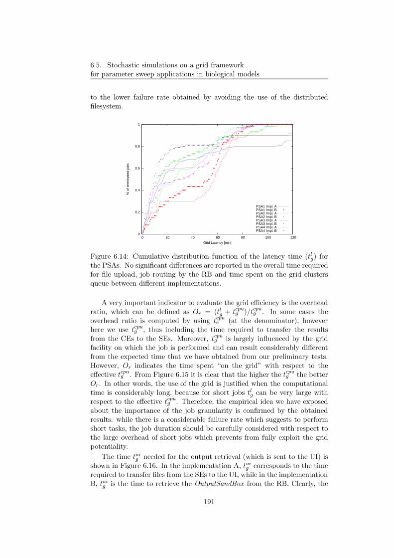
6.5. Stochastic simulations on a grid frameworkfor parameter sweep applications in biological models
to the lower failure rate obtained by avoiding the use of the distributedfilesystem.
0
0.2
0.4
0.6
0.8
1
0 20 40 60 80 100 120
% o
f ter
min
ated
jobs
Grid Latency [min]
PSA1 Impl. APSA1 Impl. BPSA2 Impl. APSA2 Impl. BPSA3 Impl. APSA3 Impl. BPSA4 Impl. APSA4 Impl. B
Figure 6.14: Cumulative distribution function of the latency time (tlg) forthe PSAs. No significant differences are reported in the overall time requiredfor file upload, job routing by the RB and time spent on the grid clustersqueue between different implementations.
A very important indicator to evaluate the grid efficiency is the overheadratio, which can be defined as Or = (tlg + tcpu
g )/tcpug . In some cases the
overhead ratio is computed by using tcpue (at the denominator), however
here we use tcpug , thus including the time required to transfer the results
from the CEs to the SEs. Moreover, tcpug is largely influenced by the grid
facility on which the job is performed and can result considerably differentfrom the expected time that we have obtained from our preliminary tests.However, Or indicates the time spent “on the grid” with respect to theeffective tcpu
g . From Figure 6.15 it is clear that the higher the tcpug the better
Or. In other words, the use of the grid is justified when the computationaltime is considerably long, because for short jobs tlg can be very large withrespect to the effective tcpu
g . Therefore, the empirical idea we have exposedabout the importance of the job granularity is confirmed by the obtainedresults: while there is a considerable failure rate which suggests to performshort tasks, the job duration should be carefully considered with respect tothe large overhead of short jobs which prevents from fully exploit the gridpotentiality.
The time tuig needed for the output retrieval (which is sent to the UI) is
shown in Figure 6.16. In the implementation A, tuig corresponds to the time
required to transfer files from the SEs to the UI, while in the implementationB, tui
g is the time to retrieve the OutputSandBox from the RB. Clearly, the
191
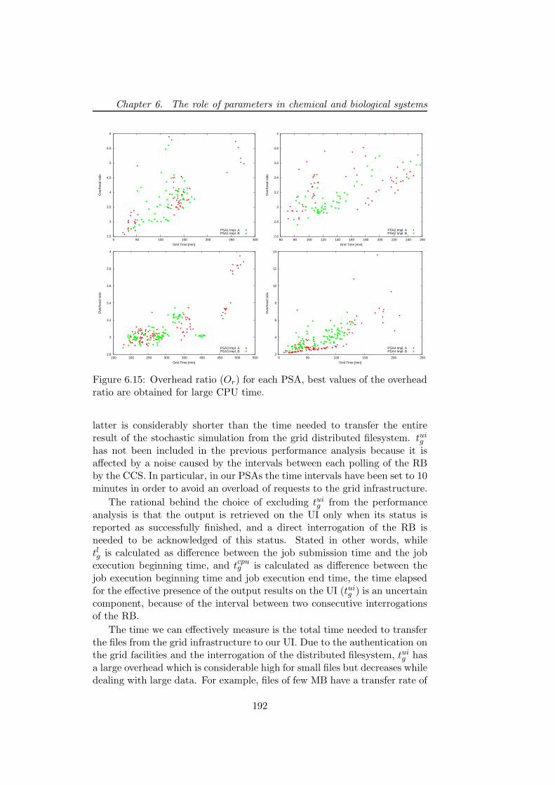
Chapter 6. The role of parameters in chemical and biological systems
2.5
3
3.5
4
4.5
5
5.5
6
0 50 100 150 200 250 300
Ove
rhea
d ra
tio
Grid Time [min]
PSA1 Impl. APSA1 Impl. B
2.6
2.8
3
3.2
3.4
3.6
3.8
4
60 80 100 120 140 160 180 200 220 240 260
Ove
rhea
d ra
tio
Grid Time [min]
PSA2 Impl. APSA2 Impl. B
2.8
3
3.2
3.4
3.6
3.8
4
150 200 250 300 350 400 450 500 550
Ove
rhea
d ra
tio
Grid Time [min]
PSA3 Impl. APSA3 Impl. B
2
4
6
8
10
12
14
0 50 100 150 200 250
Ove
rhea
d ra
tio
Grid Time [min]
PSA4 Impl. APSA4 Impl. B
Figure 6.15: Overhead ratio (Or) for each PSA, best values of the overheadratio are obtained for large CPU time.
latter is considerably shorter than the time needed to transfer the entireresult of the stochastic simulation from the grid distributed filesystem. tui
g
has not been included in the previous performance analysis because it isaffected by a noise caused by the intervals between each polling of the RBby the CCS. In particular, in our PSAs the time intervals have been set to 10minutes in order to avoid an overload of requests to the grid infrastructure.
The rational behind the choice of excluding tuig from the performance
analysis is that the output is retrieved on the UI only when its status isreported as successfully finished, and a direct interrogation of the RB isneeded to be acknowledged of this status. Stated in other words, whiletlg is calculated as difference between the job submission time and the jobexecution beginning time, and tcpu
g is calculated as difference between thejob execution beginning time and job execution end time, the time elapsedfor the effective presence of the output results on the UI (tui
g ) is an uncertaincomponent, because of the interval between two consecutive interrogationsof the RB.
The time we can effectively measure is the total time needed to transferthe files from the grid infrastructure to our UI. Due to the authentication onthe grid facilities and the interrogation of the distributed filesystem, tui
g hasa large overhead which is considerable high for small files but decreases whiledealing with large data. For example, files of few MB have a transfer rate of
192
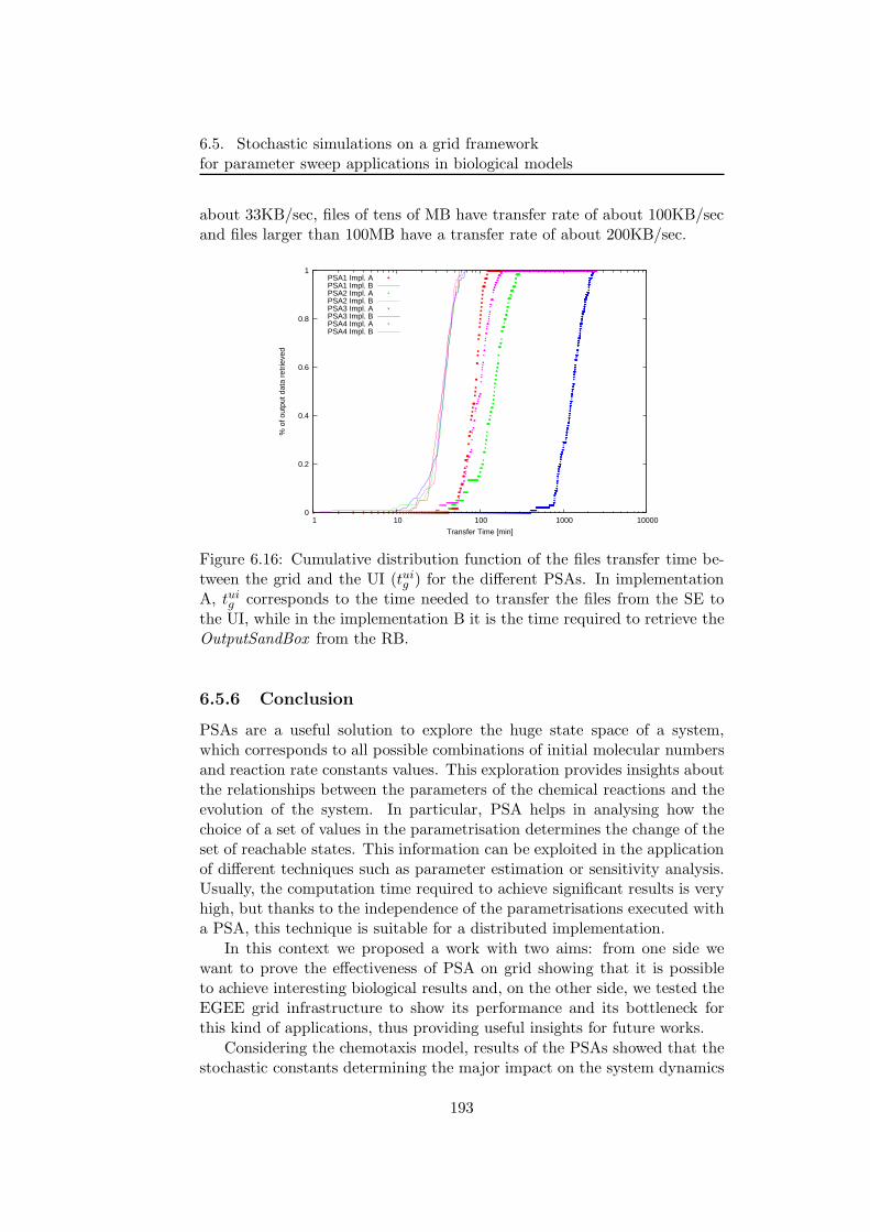
6.5. Stochastic simulations on a grid frameworkfor parameter sweep applications in biological models
about 33KB/sec, files of tens of MB have transfer rate of about 100KB/secand files larger than 100MB have a transfer rate of about 200KB/sec.
0
0.2
0.4
0.6
0.8
1
1 10 100 1000 10000
% o
f out
put d
ata
retr
ieve
d
Transfer Time [min]
PSA1 Impl. APSA1 Impl. BPSA2 Impl. APSA2 Impl. BPSA3 Impl. APSA3 Impl. BPSA4 Impl. APSA4 Impl. B
Figure 6.16: Cumulative distribution function of the files transfer time be-tween the grid and the UI (tui
g ) for the different PSAs. In implementationA, tui
g corresponds to the time needed to transfer the files from the SE tothe UI, while in the implementation B it is the time required to retrieve theOutputSandBox from the RB.
6.5.6 Conclusion
PSAs are a useful solution to explore the huge state space of a system,which corresponds to all possible combinations of initial molecular numbersand reaction rate constants values. This exploration provides insights aboutthe relationships between the parameters of the chemical reactions and theevolution of the system. In particular, PSA helps in analysing how thechoice of a set of values in the parametrisation determines the change of theset of reachable states. This information can be exploited in the applicationof different techniques such as parameter estimation or sensitivity analysis.Usually, the computation time required to achieve significant results is veryhigh, but thanks to the independence of the parametrisations executed witha PSA, this technique is suitable for a distributed implementation.
In this context we proposed a work with two aims: from one side wewant to prove the effectiveness of PSA on grid showing that it is possibleto achieve interesting biological results and, on the other side, we tested theEGEE grid infrastructure to show its performance and its bottleneck forthis kind of applications, thus providing useful insights for future works.
Considering the chemotaxis model, results of the PSAs showed that thestochastic constants determining the major impact on the system dynamics
193
Chapter 6. The role of parameters in chemical and biological systems
are c8, c37 and c49. These constants control, respectively, the addition of thefourth methyl group to the MCP, the unbinding of the ligand from the MCPwith 4 methyl groups, and the phosphorylation of CheA protein bound tothe MCP complex with MCP in the highest methylated state. The evidencethat the three constants are involved in controlling processes in the highlyMCP methylated state underlines the role of the MCP methylations for thefunctioning of the system.
The EGEE grid proved to be a useful solution for the distribution ofPSAs concerning the analysis of the biochemical systems dynamics by meansof stochastic simulations. The efficiency of this platform has been demon-strated during of our middle-size test and, considering that the more inten-sive the computation the more scalable the infrastructure, grid computingcan be considered a suitable technology to exploit in the context of largescale biological model analysis. However, due to the high rate of failure, acapable submission and monitoring environment should be set-up in orderto appropriately manage the volume of data. Moreover, to our experience,the granularity of the submitted jobs and the use of the SE for managingfiles are element to carefully consider while using the grid infrastructure.
In this work, we compared the grid performances between two imple-mentations: implementation A, in which the entire results of the stochasticsimulations are first retrieved from the SEs and then analysed; implemen-tation B, in which the model dynamics are analysed during the simulationphase and only the results of the analysis are retrieved. Implementation Ais useful when the complete numerical data of the simulations need to besaved. In implementation B, the SEs have not been used and this deter-mined an increase of the grid performances. As a consequence, these resultsencourage the development of a tool for the analysis of model dynamicsbehaviour, with one (or more) parameters perturbed, distributed over thegrid within the PSA and avoiding the retrieval of the whole numerical datarepresenting the simulations.
A possible future development of this work consists in the extension ofthe range of variation for the stochastic constants, in order to identify theboundaries of the “wild type” behaviour of the system, that is, to identify thevalues of the stochastic constants in which the system’s behaviour actuallychanges and might show other biologically relevant dynamics. Moreover, totest the robustness of the biological model, we plan to apply PSAs with aparametrisation where also the initial molecular quantities are changed. Inconclusion, good performances provided by the grid framework encourageto use this architecture to develop a sensitivity analysis tool for stochasticbiochemical systems, since also in this field, a large number of simulationsneed to be performed in order to quantify how much the parameters of themodel can affect the system’s behaviour, e.g., to help in recognizing thefragilities or the robustness of the system.
194
Chapter 7
Conclusion and future work
The work presented in this thesis has been motivated by the need to developnovel methods for the stochastic simulation and analysis of discrete modelsfor biochemical systems.
To this aim, we first considered DPPs [162], a variant of P systems [154]that can be used to model chemical, biological and ecological systems. DPPsrely on the definition of a topological structure (i.e., the membrane struc-ture), that is suitable to represent the hierarchical organisation of the com-partments composing a biochemical system; moreover, they use rewritingrules to describe the chemical reactions that modify the chemical speciesinvolved in the system, which are in turn represented as multisets of ob-jects. In DPPs probabilities are associated to the rules, and these valuesvary according to the system state. By exploiting these values, it is possibleto provide a description of the system’s dynamics, that is, DPPs allow toreproduce the stochastic variations of the elements (i.e. chemical species)occurring in the system. However, this description is only qualitative, inthe sense that an effective (physical) time streamline cannot be directlyassociated to the evolution steps of the system.
On the other hand, a quantitative description of a system’s dynamics,in which a time length is associated to each evolution step, can be actuallyprovided by using stochastic simulation algorithms. Among others, one ofthe most efficient procedure of this type is represented by the tau-leaping al-gorithm [26]. Though it has been shown that tau-leaping can be successfullyused to generate the dynamics of biochemical systems in a very accurate way,one of its limitations is related to its applicability only to systems enclosedwithin a single volume.
To solve these problems, starting from the notions of DPPs and tau-leaping algorithm, we have developed a novel method which combines theirsuitable features for the description and simulation of biochemical systems,while overcoming their limitations. So doing, we are now able to obtainquantitative and accurate simulations of the dynamics of biochemical sys-
195
Chapter 7. Conclusion and future work
tems composed by many volumes. This novel procedure is called τ -DPP[30]: it consists in a modified tau-leaping algorithm which is enclosed insideeach compartment defined in the membrane structure of DPPs.
A second version of this framework, called Sτ -DPP [29], has then beenintroduced. Sτ -DPP owns all features of τ -DPP and, in addition, it considersthe size of both molecules and compartments, to the purpose of buildingrealise more realistic models and obtain more accurate simulation resultsfor biological systems.
The stochastic framework for multivolume systems could be further im-proved by considering diffusive processes inside the compartments, which isvery important in order to characterise the actual localizations of the chem-icals involved in the modelled systems. Moreover, since these simulationmethods aim at a close description of the biological reality, compartmentswhose size changes during the evolution should also be taken into consider-ation, especially when dealing with cellular processes spanning the cell cycleperiod.
Another biological aspect that is worth considering is the influence ofmembrane potential over the processes occurring in the system. For in-stance, in neurons, the open and close states of ion channels are controlledby the existence of a membrane potential and its variations.
Both algorithms, τ -DPP and Sτ -DPP, have been implemented in C lan-guage exploiting MPI to handle parallel computations. So doing, the simu-lation of a model can be executed on parallel architectures, by assigning toeach node (or processor) a single compartment, thus reducing the computa-tional load of the whole simulation. The efficiency of τ -DPP and Sτ -DPPcan be even improved by using alternative implementations, with the aim ofdistributing the simulations on parallel architectures like grid, or on paralleldevices like GPUs by using CUDA libraries.
Different examples of biological and chemical systems, described throughdiscrete models and simulated using the τ -DPP algorithm, have been pre-sented in this thesis.
We have described the Ras/cAMP/PKA pathway in the yeast S. cere-visiae, focusing on the cytoplasmic regulators of the pathway, and provid-ing stochastic simulations of the synthesis of cAMP and of the cytoplasmicquantities of the pivotal complexes. As a future development, we plan toconstruct an accurate map of other related cellular phenomena, such as theresponse of this pathway to nutrients and to intracellular acidification, itsconnections with other pathways co–involved in glucose signalling, and thedownhill nuclear expression of target genes. In particular, in order to gaina higher biological relevance of our model, we will include the Gpr1/Gpa2pathway, which is a specific signalling mechanism that responds only to highglucose concentration, and operates in an addictive redundant way with Rasprotein to activate pathway. We believe that establishing the pivotal rolesof the different components in the Ras/cAMP/PKA pathway in yeast might
196
have a positive outcome for the elucidation of similar components in highereukaryotes. For instance, it is well known that the protein neurofibromin1 (NF1), acting as tumor suppressor in human cells, is homologous to theproteins of the Ira family, and it has been shown to contain a GAP relateddomain which regulates Ras [10].
Then, we have proposed a multivolume model implementing a syntheticmulticellular clock [67], obtained by coupling the repressilator system withbacterial quorum sensing. This intercellular communication mechanism isable to lead the local genetic oscillators (within a noisy and nonidenticalpopulation) to global oscillatory rhythms. The results of the simulationsperformed by means of τ -DPP have shown the oscillatory dynamics of theproteins involved in a single cell. Moreover, we have investigated the effectsof the quorum sensing signal, focusing on the communication mechanismfrom the cell to the environment and vice-versa. It would be interesting toextend this work in order to check whether a more complex system, consist-ing of a population of coupled cells, can show (emergent) synchronisationevents with respect to the oscillations of the three repressor proteins andthe quorum sensing protein. Since the modelling and simulation approachwe have used is stochastic, the gain of such a synchronised behaviour in anoisy system is harder than doing this with a deterministic approach.
The last biological application of τ -DPP proposed in this thesis concernsa very detailed mechanistic model of the bacterial chemotaxis pathway, thattakes into account all proteins (and their respective interactions) involvedin both signalling and response. In particular, all post-translational mod-ifications of proteins, such as methylation and phosphorylation, have beenconsidered because of their relevant roles in the feedback control mecha-nisms governing this pathway. We have investigated the dynamics of thepivotal protein involved in chemotaxis, CheYp, under different conditions,such as the deletion of other chemotactic proteins, the addition of distinctamounts of external ligand, the effect of different methylation states. Then,we have investigated the possible influence of stochastic fluctuations of thechemotactic protein CheYp with respect to the running and tumbling mo-tion of bacterial cells, by considering an increasing number of flagella in theindividual bacterium. To this aim, we have defined a procedure to identifythe synchronisation of rotation of each and every flagella: we have assumedthat the cell is sensitive to a threshold level of CheYp, which is evaluated asthe mean value of CheYp at steady state. Because of stochastic fluctuations,the amount of CheYp will randomly switch from below to above this value,thus reversing the rotation of each flagellum from counterclockwise to clock-wise mode. Our results have demonstrated the importance of stochasticity,showing the link between the synchronisation of all flagella to the stochasticfluctuations of CheYp, as the core component that stands at the basis ofchemotactic motions. This model might be improved in order to considerother relevant features of bacterial chemotaxis. For instance, the gradient
197
Chapter 7. Conclusion and future work
of CheYp that can be present inside the cytoplasm – due to the diffusionfrom the area of its phosphorylation (close to chemotactic receptors) to thearea of its activity (around the flagellar motors) – can be a significant as-pect in chemotaxis, together with the localization of CheZ (that controls thedephosphorylation of CheYp) and of the flagella around the cell [110].
As a final application, we have considered the framework of chemicalcomputing for the implementation of logic gates and circuits. The chemicalcomputing approaches present in literature define simple logic components assets of chemical reactions enclosed in a single volume, which can be simulatedby means of classic stochastic algorithms. τ -DPP provides an extension ofthese approaches, since it allows to simulate a set of simple logic componentsby splitting each of them in separate – but communicating – compartments.So doing, we can both reproduce the behaviour of every component, andpropagating the output/input signals by sending/receiving molecules amongthe distinct compartments.
In particular, we started by simulating two simple logic gates, NANDand XOR. These gates represent the basic elements for the implementationof more complex computing devices. In fact, by composing a number ofNAND or XOR logic gates, arranged according to a particular structure, itis possible to represent any boolean function. Then, we have shown howto model and simulate the Fredkin gate and Fredkin circuits. A possibleimprovement to the implementation and simulation of the presented gatesand circuits might include, for instance, the test of different sets of stochasticconstants for the chemical reactions, in order to reduce the delay generatedduring the computation.
A different example of chemical computing that we have presented withinthe τ -DPP framework, consists in the simulation of the register machineinstructions. We have shown the modelling of the SUB instruction as asystem composed by two membranes, governed by a conditional behaviourthat checks whether a register is zero or not. We have then presented theresults obtained by simulating the SUBADD module.
The results obtained from these applications have shown a close cor-respondence between τ -DPP and the chemical reacting systems occurringinside micro reactors [87]; this can be considered a preliminary step towardsa real implementation of τ -DPP by means of the microflow reactors tech-nology.
In the second part of the thesis we have explained the important roleof parameters in biochemical systems, by focusing on the set of stochasticconstants associated to the reactions. We have described two techniqueswhose aim are, on the one hand, to calibrate the parameters values by meansof optimisation algorithms and, on the other hand, to explore the parametersspace by considering a very large set of independent simulations. Thesemethods are called parameter estimation and parameter sweep application,
198
respectively.For the first method, we have compared the performances of genetic
algorithms and particle swarm optimizer. The experimental results thatwe have obtained hint that the canonical implementation of particle swarmoptimizer is a suitable optimization method for parameter estimation. Thevalues of the constants returned by particle swarm optimizer have allowedto faithfully reconstruct the behavior of simple chemical systems.
Some possible improvements to the proposed optimisation methods in-clude the use of further operators of genetic algorithms as, for instance,Laplace Crossover, Makinen, Periaux and Toivanen Mutation, Non-UniformMutation [48], or other models of particle swarm optimizer, like the imple-mentations with structured populations, with various different neighbour-hood structures or with more than two basins of attraction (in addition tothe local and global best positions).
Another possible improvement concerns the fitness function. Indeed, thedefinition of a suitable fitness function is an intrinsically difficult task forparameter estimation of biochemical systems, for several reasons. First ofall, if we exploit stochastic simulation algorithms for the fitness calculation,then it is very unlike to reach the (ideal) value of zero because of the stochas-tic fluctuations of the estimated time series. Moreover, the same individualwill generally have different fitness values each time it is evaluated. Thesedrawbacks could be mitigated by executing many times the simulation al-gorithm and calculating averages, but this might be very time consumingin some cases and could raise serious problems when the target dynamicsshows an oscillating behavior (averages may flatten oscillations).
These problems could be solved by introducing a novel version of thefitness function. For instance, the time axis can be divided into subintervals,and the optimization can be performed by incrementally extending the timeinterval considered for the fitness calculation. Furthermore, different weightscan be assigned to the regions of the dynamics that show distinct behaviours,according to some previous knowledge of the system. In addition, a differentweight could be assigned to the various species involved in the chemicalreactions under consideration, according to the relevance they hold withinthe system.
Finally, in the last part of the thesis, the parameter sweep applicationimplemented on a grid framework has been presented. As a case study, wehave applied this technique to the bacterial chemotaxis model, comparingthe results obtained from the application of 4 different configurations ofthe parameter sweep. The obtained results have shown the suitability ofthe grid framework for this kind of analysis for biochemical systems, andsuggest to implement parameter sweep applications that avoids the retrievalof huge numerical data since the data transfer represents the main cause ofjob failure.
Parameter sweep application can even be exploited to develop a novel
199
Chapter 7. Conclusion and future work
sensitivity analysis approach for stochastic biochemical models. In mathe-matical modelling of biological or biochemical systems, sensitivity analysisis used to quantify how much the parameters of the model can affect the sys-tem’s behaviour, e.g., to help in recognizing the fragilities or the robustnessof the system. Though it has been traditionally applied to deterministiccontinuous models, theories and tools for parametric sensitivity of discretestochastic systems have recently been defined [82, 166], with the aim ofcapturing the relevant stochastic effects which can occur in small systems.Taking advantage of these theories, we plan to develop a similar analysismethodology within the framework of τ -DPP. So doing, by exploiting allrelevant characteristics of membrane systems (discreteness, multicompart-mental structure), integrated with the efficiency of stochastic simulationalgorithms, and extended with tools for the estimation and the analysis ofsystem’s parameters, the framework presented in this thesis can indeed beconsidered an useful and successful approach for the stochastic modellingand simulation of biochemical systems.
200
Bibliography
[1] T. Ahn, P. Wang, L. Watson, Y. Cao, C. Shaffer, and W. Baumann.Stochastic Cell Cycle Modeling for Budding Yeast. In G. Wainer,M. Chinni, P. Roman, H. Rajaei, B. Zeigler, and C. Ribbens, edi-tors, Proc. of Spring Simulation Multiconference: HPC, pages 569–574, 2009.
[2] H. R. Akcakaya and P. Sjogren-Gulve. Population viability analysisin conservation planning: an overview. Ecol. Bull., 48:9–21, 2000.
[3] B. Alberts, A. Johnson, J. Lewis, M. Raff, K. Roberts, and P. Walter.Molecular Biology of the Cell. Garland Science, 4th. edition, 2002.
[4] A. Alhazov, R. Freund, and M. Oswald. Cell/symbol complexity oftissue p systems with symport/antiport rules. Int. J. Found. Comput.S., 17(1):3–25, 2006.
[5] U. Alon, M. G. Surette, N. Barkai, and S. Leibler. Robustness inbacterial chemotaxis. Nature, 397(6715):168–171, 1999.
[6] A. Arkin, J. Ross, and H. H. McAdams. Stochastic kinetic analysisof developmental pathway bifurcation in phage λ-infected Escherichiacoli cells. Genetics, 149:1633–1648, 1998.
[7] A. Auger, P. Chatelain, and P. Koumoutsakos. R-leaping: Accelerat-ing the stochastic simulation algorithm by reaction leaps. J. Chem.Phys., 125:084103, 2006.
[8] J. Baker. Adaptive selection methods for genetic algorithms. In Pro-ceedings of the 1st International Conference on Genetic Algorithmstable of contents, pages 101–111. L. Erlbaum Associates Inc. Hillsdale,NJ, USA, 1985.
[9] F. K. Balagadde, H. Song, J. Ozaki, C. H. Collins, M. Barnet, F. H.Arnold, S. R. Quake, and L. You. A synthetic Escherichia colipredator-prey ecosystem. Mol. Syst. Biol., 4:187, 2008.
201
Bibliography
[10] R. Ballester, D. Marchuk, M. Boquski, R. Letcher, M. Wigler, andF. Collins. The NF1 locus encodes a protein functionally related tomammalian GAP and yeast Ira proteins. Cell, 63(4):851–859, 1999.
[11] N. Barkai and S. Leibler. Robustness in simple biochemical networks.Nature, 387(6636):913–917, 1997.
[12] M. D. Baroni, E. Martegani, P. Monti, and L. Alberghina. Cell sizemodulation by CDC25 and RAS2 genes in Saccharomyces cerevisiae.Mol. Cell. Biol., 9:2715–2723, 1989.
[13] D. Besozzi, P. Cazzaniga, M. Dugo, G. Mauri, and D. Pescini. Stochas-tic modelling and parameter estimation of bacterial chemotaxis. Posterat Eighth International Conference on Information Processing in Cellsand Tissues (IPCAT), Ascona, Switzerland, April 2009.
[14] D. Besozzi, P. Cazzaniga, M. Dugo, D. Pescini, and G. Mauri. Astudy on the combined interplay between stochastic fluctuations andthe number of flagella in bacterial chemotaxis. EPTCS, 6:47–62, 2009.
[15] D. Besozzi, P. Cazzaniga, G. Mauri, D. Pescini, and L. Vanneschi. Acomparison of genetic algorithms and particle swarm optimization forparameter estimation in stochastic biochemical systems. In Proc. ofEvoBIO, number 5483 in Lecture Notes on Computer Science, pages116–127, 2009.
[16] D. Besozzi, P. Cazzaniga, D. Pescini, and G. Mauri. Seasonal variancein P system models for metapopulations. Prog. Nat. Sci., 17(4):392–400, 2007.
[17] D. Besozzi, P. Cazzaniga, D. Pescini, and G. Mauri. Modellingmetapopulations with stochastic membrane systems. Biosystems,91(3):499 – 514, 2008.
[18] D. Besozzi, P. Cazzaniga, D. Pescini, and G. Mauri. Algorithmic Bio-processes, chapter A Multivolume Approach to Stochastic Modellingwith Membrane Systems. in press.
[19] L. Bianco, F. Fontana, and V. Manca. P systems with reaction maps.Int. J. Found. Comput. S., 17(1):27–48, 2006.
[20] L. Bianco, D. Pescini, P. Siepmann, N. Krasnogor, F. Romero-Campero, and M. Gheorghe. Towards a p systems pseudomonasquorum sensing model. In H. e. a. E. Hoogeboom, editor, Proc. of7th International Workshop on Membrane Computing, volume 4361of LNCS, 2006.
202
Bibliography
[21] A. Bren and M. Eisenbach. Changing the direction of flagellar rotationin bacteria by modulating the ratio between the rotational states ofthe switch protein flim. J. Mol. Biol., 312(4):699–709, 2001.
[22] R. Buyya, D. Abramson, and J. Giddy. Nimrod/g: an architecturefor a resource management and scheduling system in a global compu-tational grid. In Proc. Fourth International Conference/Exhibition onHigh Performance Computing in the Asia-Pacific Region, volume 1,pages 283–289 vol.1, 2000.
[23] S. Cagnoni, L. Vanneschi, A. Azzini, and A. Tettamanzi. A critical as-sessment of some variants of particle swarm optimization. In EuropeanWorkshop on Bio-inspired algorithms for continuous parameter opti-misation, EvoNUM’08, LNCS, pages 565–574. Springer Verlag, 2008.
[24] S. Campana, D. Rebatto, and A. Sciab. Experience with the gliteworkload management system in atlas monte carlo production on lcg.J. Phys. Conf. Ser., 119, 2008.
[25] Y. Cao, D. T. Gillespie, and L. R. Petzold. Avoiding negative pop-ulations in explicit Poisson tau-leaping. J. Chem. Phys., 123:054104,2005.
[26] Y. Cao, D. T. Gillespie, and L. R. Petzold. Efficient step size selectionfor the tau-leaping simulation method. J. Chem. Phys., 124:044109,2006.
[27] B. Carter and P. Sudbery. Small-sized mutants of Saccharomyces cere-visiae. Genetics, 96:561–566, 1980.
[28] H. Casanova, F. Berman, G. Obertelli, and R. Wolski. The applesparameter sweep template: User-level middleware for the grid. In Proc.ACM/IEEE 2000 Conference Supercomputing, pages 60–60, 2000.
[29] P. Cazzaniga, G. Mauri, L. Milanesi, E. Mosca, and D. Pescini. Anovel variant of tissue p systems for the modelling of biochemical sys-tems. In G. Paun, M. Perez-Jimenez, A. Riscos-Nunez, G. Rozenberg,and A. Salomaa, editors, Proc. of the 10th International Workshop onMembrane Computing, 2009.
[30] P. Cazzaniga, D. Pescini, D. Besozzi, and G. Mauri. Tau leapingstochastic simulation method in P systems. In H. J. Hoogeboom,G. Paun, G. Rozenberg, and A. Salomaa, editors, Proc. of the 7thInternational Workshop on Membrane Computing, volume 4361, pages298–313. LNCS, 2006.
203
Bibliography
[31] P. Cazzaniga, D. Pescini, D. Besozzi, G. Mauri, S. Colombo,and E. Martegani. Modeling and stochastic simulation of theras/camp/pka pathway in the yeast saccharomyces cerevisiae evi-dences a key regulatory function for intracellular guanine nucleotidespools. J. Biotechnol., 133(3):377–385, 2008.
[32] P. Cazzaniga, D. Pescini, F. Romero-Campero, D. Besozzi, andG.Mauri. Stochastic approaches in P systems for simulating biologicalsystems. In M. A. Gutierrez-Naranjo, G. Paun, A. Riscos-Nunez,and F. J. Romero-Campero, editors, Proc. of the 4th Brainstorm-ing Week on Membrane Computing, volume I of RGNC REPORT02/2006, pages 145–164, Sevilla, January 30 - February 3 2006. FenixEditora.
[33] Cellware. http://www.cellware.org.
[34] A. Chatterjee and P. Siarry. Nonlinear inertia weight variation fordynamic adaptation in particle swarm optimization. Comp. Oper.Res., 33(3):859–871, 2006.
[35] A. Chatterjee, D. G. Vlachos, and M. A. Katsoulakis. Binomial dis-tribution based tau-leap accelerated stochastic simulation. J. Chem.Phys., 122:024112, 2005.
[36] F. Ciocchetta and J. Hillston. Bio-pepa: an extension of the processalgebra pepa for biochemical networks. Electr. Notes Theor. Comput.Sci., 194(3):103–117, 2008.
[37] S. Colombo, P. Ma, L. Cauwenberg, J. Winderickx, M. Crauwels,A. Teunissen, D. Nauwelaers, J. H. de Winde, M.-F. Gorwa, D. Colav-izza, and J. M. Thevelein. Involvement of distinct G-proteins, Gpa2and Ras, in glucose- and intracellular acidification-induced cAMP sig-nalling in the yeast Saccharomyces cerevisiae. Embo. J., 17:3326–3341,1998.
[38] S. Colombo, D. R. J. M. Thevelein, J. Winderickx, and E. Martegani.Activation state of the Ras2 protein and glucose-induced signaling inSaccharomyces cerevisiae. J. Biol. Chem., 279:46715–46722, 2004.
[39] K. A. Connors. Chemical kinetics: The study of Reaction Rates inSolution. VCH, 1990.
[40] M. J. Conroy, Y. Cohen, F. C. James, Y. G. Matsinos, and B. Maurer.Parameter estimation, reliability, and model improvement for spatiallyexplicit models of animal populations. Ecol. Appl., 5(1):17–19, 1995.
[41] Copasi. http://www.copasi.org/tiki-index.php.
204
Bibliography
[42] T. Cormen, C. Leiserson, and R. Rivest. Introduction to Algorithms.The MIT Press, Cambridge, MA, 1990.
[43] V. Danos and C. Laneve. Formal molecular biology. Theor. Comput.Sci., 325(1):69–110, 2004.
[44] L. Davis. Handbook of genetic algorithms. 1991.
[45] P. Dayan, L. Abbott, and L. Abbott. Theoretical neuroscience: Com-putational and mathematical modeling of neural systems. MIT Press,2001.
[46] K. De Jong. An analysis of the behavior of a class of genetic adaptivesystems. Dissert. Abstr. Inter., 36, 1975.
[47] A. De Wit. Spatial patterns and spatiotemporal dynamics in chemicalsystems. Adv. Chem. Phys., 109:435 – 513, 1999.
[48] K. Deep and M. Thakur. A new crossover operator for real codedgenetic algorithms. Appl. Math. Comput., 188(1):895–911, 2007.
[49] P. Dittrich. Chemical computing. In P. F. O. M. J.-P. Banatre, J.-L. Giavitto, editor, Unconventional Programming Paradigms (UPP2004), volume 3566, pages 19–32. Lecture Notes in Computer Science,2005.
[50] Dizzy. http://magnet.systemsbiology.net/software/Dizzy/.
[51] M. Dugo. Modellazione stocastica della chemiotassi batterica. Bach-elor thesis, Universita degli Studi di Milano, 2009.
[52] J. B. J. Dunning, D. J. Stewart, B. J. Danielson, B. R. Noon, T. L.Root, R. H. Lamberson, and E. Stevens. Spatially explicit populationmodels: current forms and future uses. Ecol. Appl., 5(1):3–11, 1995.
[53] C. M. Dyer, A. S. Vartanian, H. Zhou, and F. W. Dahlquist. A molec-ular mechanism of bacterial flagellar motor switching. J. Mol. Biol.,388:71–84, 2009.
[54] R. Eberhart and J. Kennedy. A new optimiser using particle swarmtheory. In Proc. of the Sixth International Symposium on Micro Ma-chine and Human Science, pages 39–43. IEEE service center, 1995.
[55] R. Eberhart and Y. Shi. Particle swarm optimization: developments,applications and resources. In Proceedings of the 2001 congress on evo-lutionary computation, volume 1, pages 81–86. Piscataway, NJ, USA:IEEE, 2001.
[56] Egee project. http://www.eu-egee.org/.
205
Bibliography
[57] J. Elf and M. Ehrenberg. Spontaneous separation of bi-stable bio-chemical systems into spatial domains of opposite phases. IEE P.Syst. Biol., 1(2):230–236, 2004.
[58] M. B. Elowitz and S. Leibler. A synthetic oscillatory network of tran-scriptional regulators. Nature, 403(6767):335–338, 2000.
[59] M. B. Elowitz, A. J. Levine, E. D. Siggia, and P. S. Swain. Stochasticgene expression in a single cell. Science, 297:1183–1186, 2002.
[60] L. Eshelman, R. Caruana, and J. Schaffer. Biases in the crossoverlandscape. In Proceedings of the third international conference on Ge-netic algorithms table of contents, pages 10–19. Morgan KaufmannPublishers Inc. San Francisco, CA, USA, 1989.
[61] L. Eshelman and J. Schaffer. Real-coded genetic algorithms and in-terval schemata. FOGA 2, pages 187–202, 1993.
[62] A. Faisal, L. Selen, and D. Wolpert. Noise in the nervous system. Nat.Rev. Neurosci., 9(4):292–303, 2008.
[63] I. Foster, C. Kesselman, and S. Tuecke. The anatomy of the grid:enabling scalable virtual organizations. Int. J. High Perform. Comput.Appl., 15:200–222, 2001.
[64] E. Fredkin and T. Toffoli. Conservative logic. Int. J. Theor. Phys.,21(3):219–253, 1982.
[65] R. Freund, G. Paun, and M. J. Perez-Jimenez. Tissue p systems withchannel states. Theor. Comput. Sci., 330(1):101 – 116, 2005.
[66] P. Frisco. The conformon-P system: a molecular and cell biology-inspired computability model. Theor. Comput. Sci., 312(2-3):295–319,2004.
[67] J. Garcia-Ojalvo, M. B. Elowitz, and S. H. Strogatz. Modeling a syn-thetic multicellular clock: repressilators coupled by quorum sensing.PNAS, 101:10955–10960, 2004.
[68] C. W. Gardiner. Handbook of Stochastic Methods: for Physics,Chemistry and the Natural Sciences (Springer Series in Synergetics).Springer, 3rd edition, 2004.
[69] C. Germain-Renaud, R. Texier, A. Osorio, and C. Loomis. Gridscheduling for interactive analysis. Stud. Health Tech. Informat.,120:25–33, 2006.
206
Bibliography
[70] S. Ghaemmaghami, W. Huh, K. Bower, R. W. Howson, A. Belle,N. Dephoure, E. K. O’Shea, and J. S. Weissman. Global analysis ofprotein expression in yeast. Nature, 425:737–741, 2003.
[71] M. Gibson. Computational methods for stochastic biological systems.PhD thesis, 2000.
[72] M. Gibson and J. Bruck. Efficient exact stochastic simulation of chemi-cal systems with many species and many channels. Journ. Phys. Chem.A, 104(9):1876–1889, 2000.
[73] D. T. Gillespie. General method for numerically simulating stochastictime evolution of coupled chemical-reactions. Journ. Comput. Phys.,22:403–434, 1976.
[74] D. T. Gillespie. Exact stochastic simulation of coupled chemical reac-tions. Journ. Phys. Chem., 81(25):2340–2361, 1977.
[75] D. T. Gillespie. Markov Processes: An Introduction for Physical Sci-entists. Academic Press, 1991.
[76] D. T. Gillespie. Stochastic simulation of chemical kinetics. Annu. Rev.Phys. Chem., 58:35–55, 2007.
[77] D. T. Gillespie and L. R. Petzold. Approximate accelerated stochas-tic simulation of chemically reacting systems. Journ. Chem. Phys.,115:1716–1733, 2001.
[78] D. T. Gillespie and L. R. Petzold. Improved leap-size selection foraccelerated stochastic simulation. Journ. Chem. Phys., 119:8229–8234,2003.
[79] D. E. Goldberg. Genetic Algorithms in Search, Optimization and Ma-chine Learning. Addison-Wesley, 1989.
[80] D. E. Goldberg. Real-coded genetic algorithms, virtual alphabets, andblocking. Compl. Syst., 5:139–167, 1990.
[81] E. Gross, D. Goldberg, and A. Levitzki. Phosphorylation of the S.cerevisiae Cdc25 in response to glucose results in its dissociation fromRas. Nature, 360:762–765, 1992.
[82] R. Gunawan, Y. Cao, L. Petzold, and F. J. Doyle. Sensitivity analysisof discrete stochastic systems. Biophys. J., 88:2530–2540, 2005.
[83] C. Guus, E. Boender, and H. Romeijn. Handbook of global optimiza-tion, chapter Stochastic methods, pages 829–869. Kluwer AcademicPublishers, 1995.
207
Bibliography
[84] S. A. Haney and J. R. Broach. Cdc25p, the guanine nucleotide ex-change factor for the Ras proteins of Saccharomyces cerevisiae, pro-motes exchange by stabilizing Ras in a nucleotide-free state. J. Biol.Chem., 269:16541–16548, 1994.
[85] I. Hanski. Metapopulation dynamics. Nature, 396:41–49, 1998.
[86] A. Hastings and C. L. Wolin. Within-patch dynamics in a metapopu-lation. Ecology, 70(5):1261–1266, 1989.
[87] S. J. Haswell, R. J. Middleton, B. O’Sullivan, V. Skelton, P. Watts, andP. Styring. The application of microreactors to synthetic chemistry.Chem. Commun., 5:391–398, 2001.
[88] F. Herrera, M. Lozano, and J. Verdegay. Tackling real-coded geneticalgorithms: Operators and tools for behavioural analysis. Artif. Intell.Rev., 12(4):265–319, 1998.
[89] J. H. Holland. Adaptation in Natural and Artificial Systems. TheUniversity of Michigan Press, Ann Arbor, Michigan, 1975.
[90] M. Howard and A. D. Rutenberg. Pattern formation inside bacteria:fluctuations due to the low copy number of proteins. Phys. Rev. Lett.,90(12):128102, 2003.
[91] M. Inda, A. Belloum, M. Roos, D. Vasunin, C. de Laat, L. Hertzberger,and T. Breit. Interactive Workflows in a Virtual Laboratory for e-Bioscience: The SigWin-Detector Tool for Gene Expression Analysis.In Second IEEE International Conference on e-Science and Grid Com-puting, 2006. e-Science’06, pages 19–19, 2006.
[92] M. Ionescu, G. Paun, and T. Yokomori. Spiking neural P systems.Fund. Inform., 71(2):279–308, 2006.
[93] V. A. A. Jansen. The dynamics of two diffusively coupled predator-prey populations. Theor. Popul. Biol., 59:119–131, 2001.
[94] V. A. A. Jansen and A. L. Lloyd. Local stability analysis of spatiallyhomogeneous solutions of multi-patch systems. J. Math. Biol., 41:232–252, 2000.
[95] S. Janson and M. Middendorf. A hierarchical particle swarm optimizerfor dynamic optimization problems. In Applications of EvolutionaryComputing, pages 513–524. Springer, 2004.
[96] P. Jorgensen, J. Nishikawa, B. Breitkreutz, and M. Tyers. Systematicidentification of pathways that couple cell growth and division in yeast.Science, 297:395–400, 2002.
208
Bibliography
[97] M. S. Jurica and B. L. Stoddard. Mind your b’s and r’s: bacterialchemotaxis, signal transduction and protein recognition. Structure,6(7):809–813, 1998.
[98] J. Kennedy. The behavior of particles. In Proceedings of the 7th In-ternational Conference on Evolutionary Programming VII, pages 581–589. Springer-Verlag London, UK, 1998.
[99] J. Kennedy and R. Eberhart. Particle swarm optimization. In Proc. ofthe IEEE International Conference on Neural Networks, volume IV,pages 1942–1948, Piscataway, NJ, 1995.
[100] B. Kernighan and D. Ritchie. The C programming language. Prentice-Hall, Inc., Englewood Cliffs, New Jersey, 1978.
[101] H. Kitano. Foundations of Systems Biology, chapter Systems Biology:Toward System-level Understanding of Biological Systems. MIT Press,Cambridge/MA, 2001.
[102] I. Korec. Small universal register machines. Theor. Comput. Sci.,168(2):267–301, 1996.
[103] E. Laure, S. Fisher, A. Frohner, C. Grandi, P. Kunszt, A. Krenek,O. Mulmo, F. Pacini, F. Prelz, J. White, M. Barroso, P. Bunic,F. Hemmer, A. D. Meglio, and A. Edlund. Programming the gridwith glite. Comp. Meth. Sci. Tech., 12(1):33–45, 2006.
[104] C. Lenzen, R. Cool, H. Prinz, J. Kuhlmann, and A. Wittinghofer.Kinetic analysis by fluorescence of the interaction between ras and thecatalytic domain of the guanine nucleotide exchange factor Cdc25Mm.Biochemistry, 37:7420–7430, 1998.
[105] A. Leporati, C. Zandron, and G. Mauri. Reversible p systems tosimulate fredkin circuits. Fund. Inform., 74(4):529–548, 2006.
[106] M. D. Levin, C. J. Morton-Firth, W. N. Abouhamad, R. B. Bourret,and D. Bray. Origins of individual swimming behavior in bacteria.Biophys. J., 74(1):175–181, 1998.
[107] R. Levins. Some demographic and genetic consequences of environ-mental heterogeneity for biological control. Bull. Ent. Soc. Amer.,71:237–240, 1969.
[108] S. Leye, J. Himmelspach, M. Jeschke, R. Ewald, and A. Uhrmacher. Agrid-inspired mechanism for coarse-grained experiment execution. InProc. 12th IEEE/ACM International Symposium on Distributed Sim-ulation and Real-Time Applications DS-RT 2008, pages 7–16, 2008.
209
Bibliography
[109] G. Li and R. M. Weis. Covalent modification regulates ligand bindingto receptor complexes in the chemosensory system of escherichia coli.Cell, 100(3):357–365, 2000.
[110] K. Lipkow, S. S. Andrews, and D. Bray. Simulated diffusion of phos-phorylated chey through the cytoplasm of escherichia coli. J. Bacte-riol., 187(1):45–53, 2005.
[111] D. Longo and J. Hasty. Dynamics of single-cell gene expression. Mol.Syst. Biol., 2(64):1–10, 2006.
[112] P. Ma, S. Wera, P. V. Dijck, and J. M. Thevelein. The PDE1-encodedlow-affinity phosphodiesterase in the yeast Saccharomyces cerevisiaehas a specific function in controlling agonist-induced cAMP signaling.Mol. Biol. Cell, 10:91–104, 1999.
[113] K. Man, K. Tang, and S. Kwong. Genetic algorithms: concepts andapplications. IEEE T. Ind. Electron., 43(5):519–534, 1996.
[114] V. Manca. The metabolic algorithm for P systems: principles andapplications. Theor. Comput. Sci., 404(1-2):142–155, 2008.
[115] D. Maravall and J. de Lope. Multi-objective dynamic optimiza-tion with genetic algorithms for automatic parking. Soft Comput.,11(3):249–257, 2006.
[116] O. Marion. Independent agents in a globalized world modelled bytissue p systems. Artif. Life Rob., 11(2):171–174, 2007.
[117] T. T. Marquez-Lago and K. Burrage. Binomial tau-leap spatialstochastic simulation algorithm for applications in chemical kinetics.J. Chem. Phys., 127(10):104101, 2007.
[118] E. Martegani, P. Cazzaniga, D. Pescini, D. Besozzi, S. Colombo, andG. Mauri. Stochastic modeling of the Ras/cAMP signal transduc-tion pathway in yeast. In Computational Methods in Systems Biology,Trento, Italy, October 18-19 2006.
[119] E. Martegani, R. Tisi, F. Belotti, S. Colombo, C. Paiardi, J. Wind-erickx, P. Cazzaniga, D. Besozzi, and G. Mauri. Identification ofan intracellular signalling complex for RAS/cAMP pathway in yeast:experimental evidences and modelling. In International SpecialisedSymposium on Yeasts, Hanasaari - Espoo, Finland, June 18-21 2006.Poster.
[120] C. Martın-Vide, G. Paun, J. Pazos, and A. Rodrıguez-Paton. Tissuep systems. Theor. Comput. Sci., 296(2):295–326, 2003.
210
Bibliography
[121] C. Martın-Vide, J. Pazos, G. Paun, and A. Rodrıguez-Paton. A newclass of symbolic abstract neural nets: Tissue p systems. In COCOON’02: Proc. of the 8th Annual International Conference on Comput-ing and Combinatorics, pages 290–299, London, UK, 2002. Springer-Verlag.
[122] N. Matsumaru, F. Centler, P. S. di Fenizio, and P. Dittrich. Chemicalorganization theory as a theoretical base for chemical computing. Int.J. Unconv. Comput., 3:285–309, 2005.
[123] H. McAdams and A. Arkin. Stochastic mechanisms in gene expression.PNAS, 94(3):814–819, 1997.
[124] B. A. Mello and Y. Tu. Perfect and near-perfect adaptation in a modelof bacterial chemotaxis. Biophys. J., 84(5):2943–2956, 2003.
[125] P. Mendes. Foundations of Systems Biology, chapter Modeling largebiochemical systems from functional genomic data: Parameter esti-mation, pages 163–168. MIT Press, Cambridge/MA, 2001.
[126] P. Mendes and D. B. Kell. On the analysis of the inverse problemof metabolic pathways using artificial neural networks. Biosystems,38(1):15–28, 1996.
[127] P. Mendes and D. B. Kell. Non-linear optimization of biochemicalpathways: applications to metabolic engineering and parameter esti-mation. Bioinformatics, 14:869–883, 1998.
[128] T. C. Meng, S. Somani, and P. Dhar. Modeling and simulation ofbiological systems with stochasticity. In Silico Biol., 4:0024, 2004.
[129] Z. Michalewicz. Genetic algorithms + data structures = evolutionprograms. Springer-Verlag London, UK, 1996.
[130] L. Milanesi, I. Merelli, G. T. P. Cozzi, and A. Orro. Handbookof Research on Computational Grid Technologies for Life Sciences,Biomedicine and Healthcare, chapter Functional genomics applicationsin grid. Medical Information Science Reference, 2009.
[131] B. L. Miller, B. L. Miller, D. E. Goldberg, and D. E. Goldberg. Geneticalgorithms, tournament selection, and the effects of noise. ComplexSyst., 9:193–212, 1995.
[132] M. B. Miller and B. L. Bassler. Quorum sensing in bacteria. Annu.Rev. Microbiol., 55:165–199, 2001.
[133] R. Milner. Communicating and mobile systems: the π-calculus. Cam-bridge Univ Pr, 1999.
211
Bibliography
[134] M. L. Minsky. Computation: finite and infinite machines. Prentice-Hall, Inc., Upper Saddle River, NJ, USA, 1967.
[135] V. Miranda and N. Fonseca. Epso best-of-two-worlds meta-heuristicapplied to power system problems. In Proc. IEEE Congress on Evolu-tionary Computation 2002, pages 1080–1085. IEEE Computer SocietyPress, 2002.
[136] A. Moilanen. SPOMSIM: software for stochastic patch occupancymodels of metapopulation dynamics. Ecol. Modell., 179:533–550, 2004.
[137] C. G. Moles, P. Mendes, and J. R. Banga. Parameter estimation inbiochemical pathways: A comparison of global optimization methods.Genome Res., 13(11):2467–2474, 2003.
[138] C. J. Morton-Firth and D. Bray. Predicting temporal fluctuations inan intracellular signalling pathway. J. Theor. Biol., 192(1):117–128,1998.
[139] C. J. Morton-Firth, T. S. Shimizu, and D. Bray. A free-energy-based stochastic simulation of the tar receptor complex. J. Mol. Biol.,286(4):1059–1074, Mar 1999.
[140] E. Mosca, P. Cazzaniga, I. Merelli, D. Pescini, L. Milanesi, andG. Mauri. Stochastic simulations on a grid framework for parame-ter sweep applications in biological models. Accepted.
[141] E. Mosca, P. Cazzaniga, D. Pescini, G. Mauri, and L. Milanesi. Astochastic, discrete model for the simulation of the action potential.In International Specialised Symposium on Yeasts, Bologna - Italy,November 24–25 2008. Poster.
[142] The MPI standard Web Page. http://www-unix.mcs.anl.gov/mpi/.
[143] H. Muhlenbein and D. Schlierkamp-Voosen. Predictive models for thebreeder genetic algorithm I. Continuous parameter optimization. Evol.Comput., 1(1):25–49, 1993.
[144] D. Muller, S. Exler, L. Aguilera-Vazquez, E. Guerrero-Martın, andM. Reuss. Cyclic AMP mediates the cell cycle dynamics of energymetabolism in Saccharomyces cerevisiae. Yeast, 20:351–367, 2003.
[145] J. D. Murray. Mathematical Biology. I: An introduction. Springer-Verlag, New York, 2002.
[146] D. Nelson and M. Cox. Lehninger Principles of Biochemistry. W. H.Freeman Company, 2004.
212
Bibliography
[147] J. R. S. Newman, S. Ghaemmaghami, J. Ihmels, D. K. Breslow, M. No-ble, J. L. DeRisi, and J. S. Weissman. Single-cell proteomic analysisof S. cerevisiae reveals the architecture of biological noise. Nature,441:840–846, 2006.
[148] R. Nicolescu, M. Dinneen, and Y. Kim. Structured modeling withhyperdag p systems. In Proc. of the 7th Brainstorming week on Mem-brane Computing, volume II, pages 85–108, 2009.
[149] H. Niederreiter. Random number generation and quasi-Monte Carlomethods. Society for Industrial and Applied Mathematics, Philadel-phia, PA, USA, 1992.
[150] J. Nikawa, S. Cameron, T. Toda, K. M. Ferguson, and M. Wigler.Rigorous feedback control of cAMP levels in Saccharomyces cerevisiae.Gene. Dev., 1:931–937, 1987.
[151] S. Olabarriaga, A. Nederveen, and B. O’Nuallain. Parameter sweepsfor functional mri research in the” virtual laboratory for e-science”project. In Proceedings of the Seventh IEEE International Symposiumon Cluster Computing and the Grid, pages 685–690. IEEE ComputerSociety Washington, DC, USA, 2007.
[152] M. R. Parsek, D. L. Val, B. L. Hanzelka, J. E. Cronan, and E. P.Greenberg. Acyl homoserine-lactone quorum-sensing signal genera-tion. PNAS, 96(8):4360–4365, 1999.
[153] G. Paun. Computing with membranes. J. Comput. Syst. Sci.,61(1):108–143, 2000. (See also Turku Center for Computer Science-TUCS Report No 208, 1998, www.tucs.fi).
[154] G. Paun. Membrane Computing. An Introduction. Springer-Verlag,Berlin, 2002.
[155] G. Paun and R. Paun. Membrane computing as a framework formodeling economic processes. In Proc. of the Seventh InternationalSymposium on Symbolic and Numeric Algorithms for Scientific Com-puting, pages 11–18. IEEE Computer Society, 2005.
[156] G. Paun, G. Rozenberg, and A. Salomaa. Membrane computingwith external output. Fund. Inform., 41(3):259–266, 2000. (Seealso Turku Center for Computer Science-TUCS Report No 218, 1998,www.tucs.fi).
[157] G. Paun, Y. Sakakibara, and T. Yokomori. P systems on graphs ofrestricted forms. Publ. Math-Debrecen, 60:635–660, 2002.
213
Bibliography
[158] A. Penttila, E. Zubko, K. Lumme, K. Muinonen, M. Yurkin, B. Draine,J. Rahola, A. Hoekstra, and Y. Shkuratov. Comparison between dis-crete dipole implementations and exact techniques. J. Quant. Spec-trosc. Radiat. Transfer, 106(1-3):417–436, 2007.
[159] M. J. Perez-Jimenez and F. J. Romero-Campero. Transactions onComputational Systems Biology VI, volume 4220/2006 of LectureNotes in Computer Science, chapter P Systems, a New ComputationalModelling Tool for Systems Biology, pages 176–197. Springer Berlin /Heidelberg, 2006.
[160] D. Pescini. Modelling, analysis and stochastic simulations of biologicalsystems. PhD thesis, Universita degli studi di Milano - Bicocca, 2008.
[161] D. Pescini, D. Besozzi, and G. Mauri. Investigating local evolutions indynamical probabilistic P systems. In Seventh International Sympo-sium on Symbolic and Numeric Algorithms for Scientific Computing(SYNASC’05), pages 440–447. IEEE Computer Press, 2005.
[162] D. Pescini, D. Besozzi, G. Mauri, and C. Zandron. Dynamical proba-bilistic P systems. Int. J. Found. Comput. S., 17(1):183–204, 2006.
[163] D. Pescini, D. Besozzi, C. Zandron, and G. Mauri. Analysis and sim-ulation of dynamics in probabilistic P systems. In N. P. A. Carbone,editor, Proc. of 11th International Workshop on DNA Computing,DNA11, volume 3892, pages 236–247, London, ON, Canada, June 6-9, 2005 2006. LNCS.
[164] D. Pescini, P. Cazzaniga, C. Ferretti, and G. Mauri. First steps to-ward a wet implementation for τ -dpp. In D. Corne, P. Frisco, G. Paun,G. Rozenberg, and A. Salomaa, editors, Proc. of the 9th InternationalWorkshop on Membrane Computing, volume 5391 of LNCS, pages355–373, 2008.
[165] C. Petri. Kommunikation mit automata. PhD thesis, Ph. D. thesis,University of Bonn, Bonn, Germany.(in German), 1962.
[166] S. Plyasunov and A. P. Arkin. Efficient stochastic sensitivity analysisof discrete event systems. J. Comp. Phys., 221:724–738, 2007.
[167] C. W. Pouton, K. M. Wagstaff, D. M. Roth, G. W. Moseley, andD. A. Jans. Targeted delivery to the nucleus. Adv. Drug. Deliver.Rev., 59(8):698–717, 2007.
[168] The p systems web page. http://psystems.disco.unimib.it/.
[169] N. Radcliffe. Equivalence class analysis of genetic algorithms. ComplexSyst., 5(2):183–205, 1991.
214
Bibliography
[170] C. V. Rao, J. R. Kirby, and A. P. Arkin. Design and diversity in bac-terial chemotaxis: a comparative study in escherichia coli and bacillussubtilis. PLoS Biol., 2(2):E49, 2004.
[171] J. M. Reed and S. H. Levine. A model for behavioral regulation ofmetapopulation dynamics. Ecol. Modell., 183:411–423, 2005.
[172] C. Reeves. Using genetic algorithms with small populations. In Pro-ceedings of the 5th International Conference on Genetic Algorithmstable of contents, pages 92–99. Morgan Kaufmann Publishers Inc. SanFrancisco, CA, USA, 1993.
[173] S. Reinker, R. M. Altman, and J. Timmer. Parameter estimationin stochastic biochemical reactions. IEE P. Syst. Biol., 153:168–178,2006.
[174] C. Reynolds. Flocks, herds and schools: A distributed behavioralmodel. In Proceedings of the 14th annual conference on Computergraphics and interactive techniques, pages 25–34. ACM New York, NY,USA, 1987.
[175] F. Rolland, J. de Winde, K. Lemaire, E. Boles, J. Thevelein, andW. J. Glucose-induced cAMP signalling in yeast requires both a G-protein coupled receptor system for extracellular glucose detection anda separable hexose kinase-dependent sensing process. Mol. Microbiol.,38:348–358, 2000.
[176] N. Rosenfeld, J. W. Young, U. Alon, P. S. Swain, and M. B. Elowitz.Gene Regulation at the Single-Cell Level. Science, 307:1962–1965,2005.
[177] S. Rudoni, S. Colombo, P. Coccetti, and E. Martegani. Role of gua-nine nucleotides in the regulation of the Ras/cAMP pathway in Sac-charomyces cerevisiae. Biochim. Biophys. Acta, 1538:181–189, 2001.
[178] T. Runarsson and X. Yao. Stochastic ranking for constrained evo-lutionary optimization. IEEE Trans. Evol. Comput., 4(3):284–294,2000.
[179] H. Salis and Y. Kaznessis. Accurate hybrid stochastic simulation of asystem of coupled chemical or biochemical reactions. J. Chem. Phys.,122:054103, 2005.
[180] G. M. Santangelo. Glucose signaling in Saccharomyces cerevisiae. Mi-crobiol. Mol. Bio. Rev., 70(1):253–282, 2006.
[181] B. E. Scharf, K. A. Fahrner, L. Turner, and H. C. Berg. Control of di-rection of flagellar rotation in bacterial chemotaxis. PNAS, 95(1):201–206, 1998.
215
Bibliography
[182] L. Shapiro and R. Losick. Dynamic spatial regulation in the bacterialcell. Cell, 100(1):89–98, 2000.
[183] Y. Shi and R. Eberhart. Parameter selection in particle swarm opti-mization. LNCS, pages 591–600, 1998.
[184] T. S. Shimizu and D. Bray. Modelling the bacterial chemotaxis recep-tor complex. Novartis Found. Symp., 247:162–77; discussion 177–81,198–206, 244–52, 2002.
[185] V. Sourjik. Receptor clustering and signal processing in e. coli chemo-taxis. Trends Microbiol., 12(12):569–576, 2004.
[186] P. A. Spiro, J. S. Parkinson, and H. G. Othmer. A model of excitationand adaptation in bacterial chemotaxis. PNAS, 94(14):7263–7268,1997.
[187] V. Stankovski and W. Dubitzky. Special section: Data mining ingrid computing environments. Future Gener. Comp. Sy., 23(1):31–33,2007.
[188] Stochkit. http://engineering.ucsb.edu/~cse/StochKit/.
[189] A. Stundzia and C. Lumsden. Stochastic simulation of coupledreaction-diffusion processes. Journ. Comput. Phys., 127(1):196–207,1996.
[190] G. Syswerda. Uniform crossover in genetic algorithms. In Proceedingsof the 3rd International Conference on Genetic Algorithms table ofcontents, pages 2–9. Morgan Kaufmann Publishers Inc. San Francisco,CA, USA, 1989.
[191] A. D. Taylor. Metapopulations, dispersal, and predator-prey dynam-ics: an overview. Ecology, 71(2):429–433, 1990.
[192] M. Thattai and A. van Oudenaarden. Intrinsic noise in gene regulatorynetworks. PNAS, 98(15):8614, 2001.
[193] J. M. Thevelein. Signal transduction in yeast. Yeast, 10:1753–1790,1994.
[194] J. M. Thevelein, L. Cauwenberg, S. Colombo, J. H. de Winde, M. Do-naton, F. Dumortier, L. Kraakman, K. Lemaire, P. Ma, D. Nauwe-laers, F. Rolland, A. Teunissen, P. V. Dijck, M. Versele, S. Wera, andJ. Winderickx. Nutrient-induced signal transduction through the pro-tein kinase A pathway and its role in the control of metabolism, stressresistance, and growth in yeast. Enzyme Microb. Technol., 26:819–825,2000.
216
Bibliography
[195] J. M. Thevelein and J. H. de Winde. Novel sensing mechanisms andtargets for the cAMP-protein kinase A pathway in the yeast Saccha-romyces cerevisiae. Mol. Microbiol., 33:904–918, 1999.
[196] T. Tian and K. Burrage. Binomial leap methods for simulatingstochastic chemical kinetics. Journ. Chem. Phys., 121:10356–10364,2004.
[197] T. Toda, S. Cameron, P. Sass, M. Zoller, and M. Wigler. Three differ-ent genes in S. cerevisiae encode the catalytic subunits of the cAMP-dependent protein kinase. Cell, 50:277–287, 1987.
[198] T. E. Turner, S. Schnell, and K. Burrage. Stochastic approaches formodelling in vivo reactions. Comput. Biol. Chem., 28:165–178, 2004.
[199] J. J. Tyson. Some further studies of nonlinear oscillations in chemicalsystems. Journ. Chem. Phys., 58:3919–3930, 1973.
[200] R. Unger and J. Moult. Genetic algorithms for protein folding simu-lations. J. Mol. Biol., 231(1):75–81, 1993.
[201] Y. D. Valle, G. Venayagamoorthy, S. Mohagheghi, J. Hernandez, andR. Harley. Particle swarm optimization: Basic concepts, variants andapplications in power systems. IEEE Trans. Evol. Comput., 12(2):171–195, 2008.
[202] G. H. Wadhams and J. P. Armitage. Making sense of it all: bacterialchemotaxis. Nat. Rev. Mol. Cell Biol., 5(12):1024–1037, 2004.
[203] W. W. Weisser, V. A. A. Jansen, and M. P. Hassell. The effectsof a pool of dispersers on host-parasitoid systems. J. Theor. Biol.,189:413–425, 1997.
[204] A. H. Wright. Genetic algorithms for real parameter optimization. InG. J. Rawlins, editor, Foundations of genetic algorithms, pages 205–218. Morgan Kaufmann, San Mateo, CA, 1991.
[205] Yeast gfp fusion localization database. http://yeastgfp.ucsf.edu/.
217