Embed Size (px)
Citation preview
Stochastic analysis
Paul Bourgade

These are lecture notes from the lessons given in the fall 2010 at Harvard University, and fall 2016 atNew York University’s Courant Institute.These notes are based on distinct references. In particular, Chapter 3 is adapted from the remarkablelecture notes by Jean Francois Le Gall [12], in French. For Chapters 2, 4 and 5, our main referencesare [13], [16] and [18]. Chapter 6 is based on [23]. For Chapter 7, references are [1] and [10]. All errorsare mine.
These are draft notes, so please send me any mathematical inaccuracies you will certainly find. I thankStephane Chretien and Guangqu Zheng for the numerous typos they found in earlier versions of thesenotes.
Table of contents
Elementary probability prerequisites 1
Motivations 5
Chapter 1. Discrete time processes 11
1. Martingales, stopping times, the martingale property for stopping times . . 2. Inequalities : Lp norms in terms of final values, number of jumps. . . . . . 3. Convergence of martingales. . . . . . . . . . . . . . . . . . . . . . . . . . .
Chapter 2. Brownian motion 19
1. Gaussian vectors . . . . . . . . . . . . . . . . . . . . . . . . . . . . . . . . . 2. Existence of Brownian motion . . . . . . . . . . . . . . . . . . . . . . . . . 3. Invariance properties . . . . . . . . . . . . . . . . . . . . . . . . . . . . . . 4. Regularity of trajectories . . . . . . . . . . . . . . . . . . . . . . . . . . . . 5. Markov properties . . . . . . . . . . . . . . . . . . . . . . . . . . . . . . . . 6. Iterated logarithm law . . . . . . . . . . . . . . . . . . . . . . . . . . . . . 7. Skorokhod’s embedding . . . . . . . . . . . . . . . . . . . . . . . . . . . . . 8. Donsker’s invariance principle . . . . . . . . . . . . . . . . . . . . . . . . .
Chapter 3. Semimartingales 37
1. Filtrations, processes, stopping times . . . . . . . . . . . . . . . . . . . . . 2. Martingales . . . . . . . . . . . . . . . . . . . . . . . . . . . . . . . . . . . 3. Finite variation processes . . . . . . . . . . . . . . . . . . . . . . . . . . . . 4. Local martingales . . . . . . . . . . . . . . . . . . . . . . . . . . . . . . . . 5. Bracket . . . . . . . . . . . . . . . . . . . . . . . . . . . . . . . . . . . . . .
Chapter 4. The Ito formula and applications 55
1. The stochastic integral . . . . . . . . . . . . . . . . . . . . . . . . . . . . . 2. The Ito formula . . . . . . . . . . . . . . . . . . . . . . . . . . . . . . . . . 3. Transcience, recurrence, harmonicity . . . . . . . . . . . . . . . . . . . . . 4. The Girsanov theorem . . . . . . . . . . . . . . . . . . . . . . . . . . . . .
Chapter 5. Stochastic differential equations 81
1. Weak and strong solutions . . . . . . . . . . . . . . . . . . . . . . . . . . . 2. The Lipschitz case . . . . . . . . . . . . . . . . . . . . . . . . . . . . . . . . 3. The Strong Markov property and more on the Dirichlet problem . . . . . . 4. The Stroock-Varadhan piecewise approximation . . . . . . . . . . . . . . . 5. Shifts in the Cameron-Martin space . . . . . . . . . . . . . . . . . . . . . .
Chapter 6. Representations 101
1. The Ito representation . . . . . . . . . . . . . . . . . . . . . . . . . . . . . 2. The Gross-Sobolev derivative . . . . . . . . . . . . . . . . . . . . . . . . . . 3. The Clark formula . . . . . . . . . . . . . . . . . . . . . . . . . . . . . . . . 4. The Ornstein-Uhlenbeck semigroup . . . . . . . . . . . . . . . . . . . . . .
iii
iv Table of contents
Chapter 7. Concentration of measure 103
1. Hypercontractivity, logarithmic Sobolev inequalities and concentration . . 2. Concentration on Euclidean spaces . . . . . . . . . . . . . . . . . . . . . . 3. Concentration on curved spaces . . . . . . . . . . . . . . . . . . . . . . . . 4. Concentration and Boolean functions . . . . . . . . . . . . . . . . . . . . .
Bibliography 119
Elementary probability prerequisites
These pages remind some important results of elementary probability theory thatwe will make use of in the stochastic analysis lectures. All the notions and resultshereafter are explained in full details in Probability Essentials, by Jacod-Protter, forexample.
Probability space
Sample space Ω Arbitrary non-empty set.σ-algebra F A set of subsets of Ω, including the empty set, stable
under complements and countable union (hencecountable intersection).
Probability measure P A function from F to [0, 1] such that P(Ω) = 1 andP(∪iAi) =
∑i P(Ai) for any disjoint elements in F .
Probability space (Ω,F ,P) A triple composed on a set Ω, a σ-algebra F ⊂ 2Ω,and a probability measure on F .
Random variable X Given a probability space (Ω,F ,P) and a metricspace (G,G), X : Ω → G is measurable in the senseX−1(g) ∈ F for any g ∈ G.
Wiener space In these lectures, Ω can be the set W of continuousfunctions from [0, 1] to R (Wiener space) vanishingat 0, F = σ(Ws, 0 6 s 6 1) is the smallest σ-algebrafor which all coordinates mappings ω → Wt(ω) =ω(t) are measurable, and G = Rd endowed with itsBorel σ-algebra.
Monotone class theorem For C ⊂ 2Ω, let σ(C) be the smallest σ-algebracontaining C (uniquely defined as an intersection ofσ-algebras is a σ-algebra). Let P and Q be two pro-bability measures on σ(C). If C is stable by inter-section and P, Q coincide on C, then P = Q.
Conditional expectation
Definition On a probability space (Ω,F ,P), given an inte-grable random variable X : Ω → G and a sub-σ-algebra G ⊂ F , a conditional expectation of X withrespect to G is any G-measurable random variableE(X | G) : ω → G such that
∫AE(X | G)(ω)dP(ω) =∫
AX(ω)dP(ω) for any A ∈ G.
Existence Given by the Radon-Nikodym theorem, hence anabsolute continuity condition. In practice, the exis-tence is often proved in a constructive way, i.e. byshowing a random variable with the desired proper-ties (e.g. the Brownian bridge).
Uniqueness In the almost sure sense, i.e. two conditional expec-tation of X with respect to G only differ on a set ofprobability measure 0.
Property E(E(X | G)) = E(X) whenever G ⊂ F .
Elementary probability prerequisites
Functional analysis
Closed operator Let F : D(F) ⊂ A → B be a linear operator, A,Bbeing Banach spaces. The operator F is said to beclosed if for any sequence of elements an ∈ D(F)converging to a ∈ A, such that F(an) → b ∈ B,a ∈ D(F) and F(a) = b : the graph of F is closed inthe direct sum A⊕ B.
Riesz representation Any element ϕ of the dual H∗ of a Hilbert space Hcan be uniquely written ϕ = 〈x, ·〉 for some x ∈ H.
Lp − Lq duality If 1/p + 1/q = 1, p, q > 0, then ‖f‖Lp =sup‖g‖Lq61〈f, g〉.
Convergence types
Almost sure On the same probability space (Ω,F ,P), Xn
converges almost surely to X if P(Xn →n→∞
X) = 1,
where the limit is in the sense of the metric of thespace G.
Lp On the same probability space (Ω,F ,P), Xn
converges to X in Lp (p > 0) if E(|Xn−X|p) →n→∞
0,
where the distance is in the sense of the metric ofthe space G, and E is the expectation with respectto P.
In probability On the same probability space (Ω,F ,P), Xn
converges to X in probability if for any ε > 0P(|Xn − X| > ε) →
n→∞0, , where the distance is
in the sense of the metric of the space G.In law On possibly distinct probability spaces, but identi-
cal image space (G,G), Xn with law Pn converges inlaw (or in distribution, weakly) to X if for any boun-ded continuous function f on G, En(f(Xn)) →
n→∞E(f(X)).
Portmanteau’s theorem Any of the following implies the convergence inlaw : (i) the test function f only needs to be Lip-schitz (ii) if G = Rd it only needs to be infini-tely differentiable (iii) for any closed subset C of G,lim supn→∞ Pn(C) 6 P(C) (iv)for any open subsetO of G, lim infn→∞ Pn(O) > P(O).
Implications
Almost sure Lp ←−(q>p>0)
Lq
↓In probability
↓In law
Partial reciprocal Convergence in probability implies the almostconvergence along a subsequence.
Paul Levy’s theorem Take G = Rd. If, for any u ∈ Rd, En(eiu·Xn) →n→∞
f(u) := E(eiu·X) and f is continuous at 0, then Xn
converges in law to X.Paul Levy : the easy impli-cation
If Xn converges in law to X, E(eiu·Xn) converges toE(eiu·X) uniformly in compact subsets of Rd.
Elementary probability prerequisites
Theorems
Strong law of large numbers For i.i.d. random variables Xi’s with finite expecta-tion, 1
n
∑n1 Xi converges almost surely to E(X1).
Central limit theorem For i.i.d. random variables Xi’s in L2, with expecta-tion µ and variance σ2, 1
σ√n
∑n1 (Xi − µ) converges
in law to a standard Gaussian random variable.
Useful lemmas
Borel-Cantelli On a probability space (Ω,F ,P), if An ∈ F and∑n P(An) <∞, then P(∩∞n=1 ∪m>n Am) = 0.
Borel-Cantelli, independentcase
On a probability space (Ω,F ,P), if An ∈ F , theAn’s are independent and
∑n P(An) = ∞, then
P(∩∞n=1 ∪m>n Am) = 1.Fatou On a probability space (Ω,F ,P), if Xn > 0, then
E(lim inf Xn) 6 lim inf E(Xn).

Motivations
It is very natural to think about these random functions imaginedby mathematicians, and that were wrongly only seen as mathema-tical curiosities.
Jean PerrinLes atomes, 1913
In the above quote, Perrin refers to his derivation of the Avogadro number : pre-vious works by Einstein, supposing that molecules move randomly, yield to a theo-retical derivation of this physical constant ; Perrin’s work gave further experimentalsupport to Einsein’s hypothesis on the particles motion.
These trajectories, known now as Brownian motions, appeared first in the workof Brown about pollen particles moving on the surface of water. They exhibit strongirregularities (infinite variation, nowhere differentiable, uncountable set of zeros) andare universal in many senses presented hereafter. These lecture notes aim to give a self-contained introduction to these random paths, through the important contributionsof Levy, Wiener, Kolmogorov, Doob, Ito, but also to show how they enlighten non-probabilistic questions, such as a the Dirichlet problem and concentration of measure.
A first approach towards Brownian motion consists in an asymptotic analysis ofrandom walks. Let Xi be independent Bernoulli random variables, i.e. P(Xi = 1) =P(Xi = −1) = 1/2. Consider the partial sum Sn =
∑ni=1 Xi. The central limit theorem
states thatSn√n
law−→ N , (0.1)
a standard Gaussian random variable. Many other questions of interest about Sn in-clude the asymptotic distribution of sup16i6n Si or |i 6 n | Si > 0| for example. Inthe case of Bernoulli random variables, these problems can be handled by combina-torial techniques involving the Catalan numbers, but for more general variables Xi inL2, what is required is a weak limit of (Sn, n > 0), the entire process.
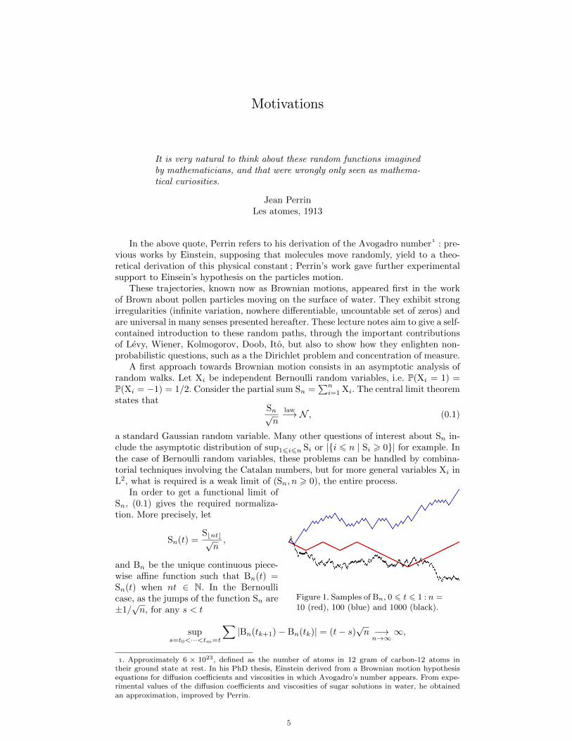
Figure 1. Samples of Bn, 0 6 t 6 1 : n =10 (red), 100 (blue) and 1000 (black).
In order to get a functional limit ofSn, (0.1) gives the required normaliza-tion. More precisely, let
Sn(t) =Sbntc√n,
and Bn be the unique continuous piece-wise affine function such that Bn(t) =Sn(t) when nt ∈ N. In the Bernoullicase, as the jumps of the function Sn are±1/√n, for any s < t
sups=t0<···<tm=t
∑|Bn(tk+1)− Bn(tk)| = (t− s)
√n −→n→∞
∞,
. Approximately 6 × 10²³, defined as the number of atoms in 12 gram of carbon-12 atoms intheir ground state at rest. In his PhD thesis, Einstein derived from a Brownian motion hypothesisequations for diffusion coefficients and viscosities in which Avogadro’s number appears. From expe-rimental values of the diffusion coefficients and viscosities of sugar solutions in water, he obtainedan approximation, improved by Perrin.
Motivations
so if the path Bn converges in some sense to a limiting object B, this is of infinitevariation on any nonempty interval.
Now, given any increasing sequence 0 = t0 < t1 < . . . , the central limit theoremyields that Bn(ti+1)− Bn(ti) converges as n→∞ to a normally distributed randomvariable with variance ti+1 − ti. More precisely,
(Bn(t1),Bn(t2)− Bn(t1), . . . ,Bn(tk+1)− Bn(tk))
law−→ (√t1N1,
√t2 − t1N2, . . . ,
√tk − tk−1Nk) (0.2)
whereN1, . . . ,Nk are independent standard Gaussian random variables. This suggeststhe following definition.
Definition. A random trajectory (Bt, t > 0) with values in R is a Brownian motionif the following four conditions are satisfied :
(i) B0 = 0 almost surely ;
(ii) for any n > 2, 0 < t1 6 · · · 6 tn, (Bt1 ,Bt2 −Bt1 , . . . ,Btn −Btn−1) is a Gaussianvector with independent components ;
(iii) for a any 0 < s < t, Bt − Bs ∼ N (0, t− s) ;
(iv) B is almost surely continuous.
Note that such a definition implies strange properties of the sample trajectory.For example, for any t > 0, s = t0 < · · · < tm = t
E
(m∑i=1
|B(ti+1)− B(ti)|
)−→n→∞
m∑i=1
√ti+1 − ti E(|N1|) > E(|N1|)
√t− s
√m,
by the Cauchy-Schwarz inequality, so as expected the L1-norm of the total variationof B on [s, t] is ∞.
More interesting than the total variation is the quadratic one : from the conver-gence in law (0.2),
E
(m∑i=1
|Bn(ti+1)− Bn(ti)|2)−→n→∞
t− s,
suggesting that the quadratic variation of a Brownian path till any time t must be t.One can even prove from the definition of the Brownian motion that
lim
( m∑i=1
|Bn(ti+1)− Bn(ti)|2 − (t− s)
)2 = 0
where the limit is in the sense of the time step going to 0 for the subdivision s =t0 < · · · < tm = t. These observations can make skeptical about the existence ofsuch paths. We will prove in Chapter 2 the following theorem, together with the firstproperties of Brownian motion. As a prerequisite, properties of discrete martingales,like Sn, will be studied in Chapter 1.
Theorem. The Brownian motion exists. More precisely, there is a measure W onC o([0, 1]) such that :
(i) W(ω(0) = 0) = 1 ;
(ii) for any n > 2, 0 < t1 6 · · · 6 tn, the projection of W by ω → (ωt1 , ωt2 −ωt1 , . . . , ωtn − ωtn−1
) is a Gaussian measure ;
Motivations
(iii) for a any 0 < s < t, the projection of W by ω → ωt−ωs is the centered Gaussianmeasure with variance t− s.
Moreover, this measure is unique and is called the Wiener measure.
Moreover, this measure is the weak limit of the random paths Bn, no matter whichdistribution the normalized Xi’s have. This is Donsker’s theorem.
Theorem. Let Bn be constructed as previously from iid Xi’s, E(Xi) = 0, E(X2i ) = 1.
Then for any bounded continuous (for the L∞ norm) functional F on C o([0, 1]),
E(F(Bn(s), 0 6 s 6 1)) −→n→∞
EW(F(B(s), 0 6 s 6 1)).
We say that the process Bn converges weakly to the Brownian motion.
To some extent, the Brownian motion is the only natural random function. Moreprecisely, take any continuous integrable random curve (Xs, s > 0) satisfying themartingale property
E(Xt | Fs) = Xs
for any s < t, where Fs = σ(Xs, s 6 t). Then a theorem by Dubins and Schwartzstates that there exists a nondecreasing F-measurable random function f such that
(Xf(s), s > 0)
is a Wiener process. This means that, up to a change of time, any martingale (whichdoes not presuppose normality) is a Brownian motion. In particular, this implies thatany martingale must either be constant or have infinite variation on any interval :there are no smooth nontrivial martingales. A study of martingales is the purpose ofChapter 3.
Chapter 4 relates martingales and the Brownian motion through the Ito calculus.This requires the definition of a stochastic integral, as the limit in probability of
Xt =
∫ t
0
a(Bs)dBs = limmesh→0
∑a(Bti)(Bti+1
− Bti)
under proper integrability assumptions for a. The Ito calculus gives the decomposition,as a stochastic integral, of transforms of the process X.
One application of the Ito formula will be the links between Brownian motion andharmonic functions.
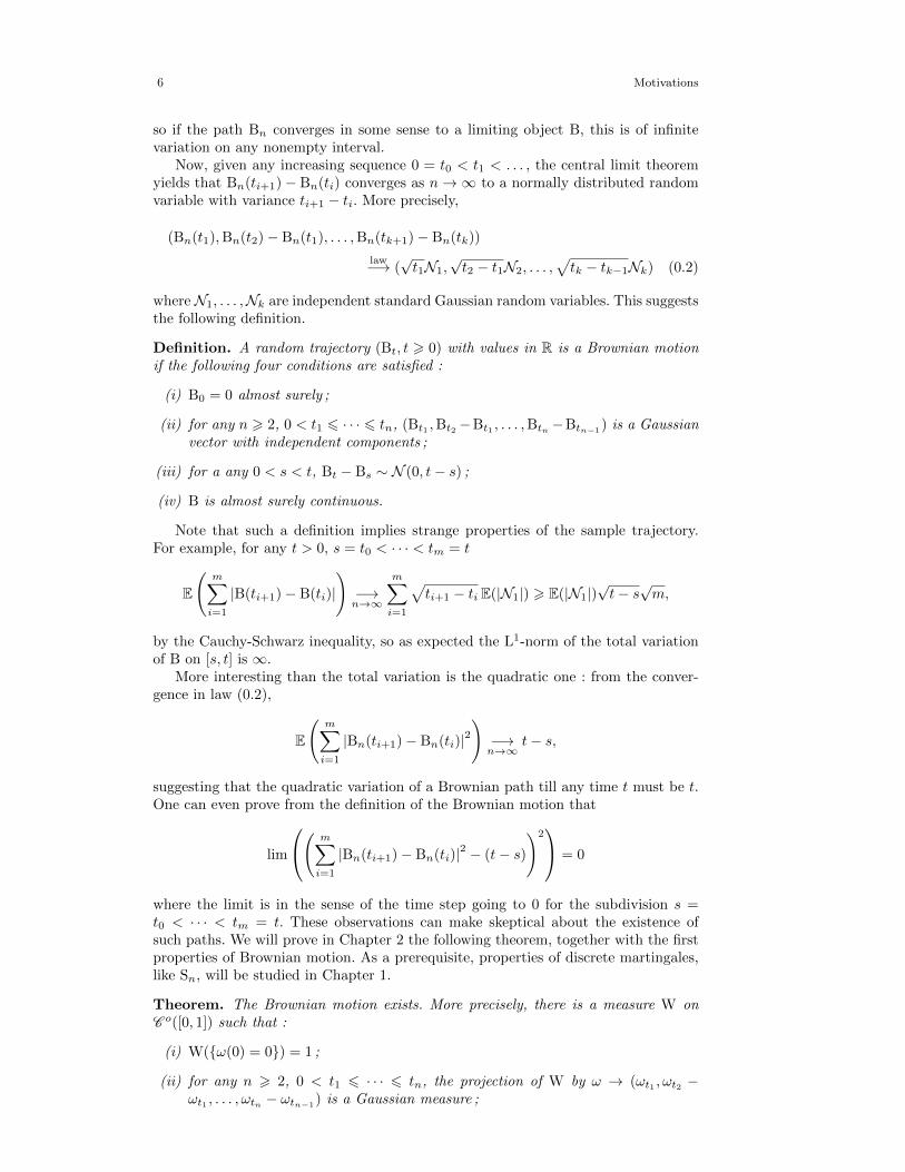
Figure 2. A bidimensional Bownianmotion till hitting the peanut frontier.
More precisely, for example,consider a connected D ⊂ R2 withsmooth boundary ∂D. The Dirichletproblem consists in finding a func-tion f : R2 → R such that
f(x) = u(x) , x ∈ ∂D,∆f = 0 , x ∈ Do.
Given a bidimensional Brownianmotion B = (B1,B2) (B1 and B2
independent Brownian motions withvalues in R), a solution to the Diri-chlet problem is
f(x) = E (u(BT) | B0 = x))
where T = inft | Bt 6∈ U. This is an example of existence results proved by proba-bilistic means.
Chapters 5 focuses on stochastic differential equations, here existence and unique-ness results for dynamics driven by a Brownian motion. Some analogies with ordinary
Motivations
differential equations appear, for example if the coefficients a and b are Lipschitzian,there is a unique path X measurable in terms of B (Xt = f(Bs, s 6 t)) such that
Xt =
∫ t
0
a(Xs)dBs +
∫ t
0
b(Xs)ds.
Surprisingly, we will see that in other situations solutions to stochastic differentialequations require less smoothness assumptions than in the deterministic case. Forexample, for
Xt = Bt +
∫ t
0
b(Xs)ds,
the measurability and boundedness of b yield to existence and uniqueness of a solution.The question, important in filtering theory, whether X is a function of B in the aboveequation will be addressed.
Chapters 6 has a more functional analysis content. First, we deal with represen-tations of random variables. For example, any F1-measurable random variable X inL2 can be written as
X =
∫ 1
0
asdBs (0.3)
for some adapted process a. This implies in particular such random variables canbe decomposed into an orthogonal basis generated by multiple stochastic integrals,the so-called chaos decomposition. Then the Gross-Sobolev derivative is introduced.This allows to investigate questions like the infinitesimal variation of F(B) (F beingF1-measurable, say) when B is perturbed by a deterministic element h, such that
h(t) =∫ t
0h(s)ds, ‖h‖2H =
∫ t0|h(s)|2ds < ∞ : for a suitable function F, by the Riesz
representation theorem, there is an element ∇F(B) ∈ H such that
limε
F(B + εh)− F(B)
ε= 〈∇F(B), h〉.
This ∇F is called the Gross Sobolev derivative of F, and will make it possible togive a complete description of what the processus a is in Ito’s representation theorem(0.3). This is important in control theory : it enables to get a random variable X byintegrating predictably along the random path B.
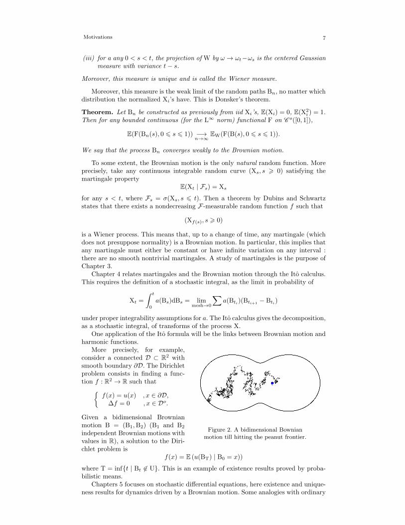
Finally, we give two applications, of independent interest, of the stochastic analy-sis. The first one is about concentration of measure, in Chapter 8. Examples of sucha concentration appear on any compact Riemannian manifold with positive Riccicurvature. For simplification here, consider the case of a n-dimensional unit sphereS n, with uniform probability measure µn. Then, for any Lipschitz function F withLipschitz constant ‖F‖L, there are constants C, c > 0 independent of n, F such that
Figure 3. Density of x1 for the uni-form measure on S n, n = 20 (pink),30 (red), 40 (blue), 50 (black).
µn |F− Eµ(F) > ε| 6 Ce−c(n−1) ε2
‖F‖2L .
In particular, choosing
F(x) = min(dist(x,M), ε)
where M is the Equator, M = x1 = 0∩Sn, yields for some constants C, c > 0
µn(dist(x,M) < ε) > 1− Ce−cnε2
,
i.e. all the mass of the uniform measureconcentrates exponentially fast around
. Fs = σ(Bu, u 6 s)
Motivations
the Equator ! How are these results related to stochastic processes ? A method to proveconcentration, initiated by Bakry and Emery, roughly speaking consists in seing theuniform measure as the equilibrium measure of a Brownian motion on the manifold :F−Eµ(F) is the different between t = 0 and t =∞ of an evolution along the Browianpath, whose differential can be controlled.
This shows an application of Brownian paths, and more generally dynamics, totime-independent probabilistic statements.

Chapter 1
Discrete time processes
Although these lectures focus on the continuous time setting, which involves phe-nomena not appearing in discrete time, this chapter aims to give the intuition andnecessary tools for the following ones. On a probability space (Ω,F ,P), an increasingsequence (Fn)n>0 of sub-σ-algebras of F is called a filtration :
F0 ⊂ F1 ⊂ · · · ⊂ Fn ⊂ . . .
Intuitively, the index n is a time and a random variable is Fn-measurable if it onlydepends on the past up to time n.
1. Martingales, stopping times, the martingale property for stopping times
Definition 1.1. A sequence (Xn)n>0 of random variables is called a ((Fn)n>0,P)-martingale if it satisfies the three following conditions, for any n > 0 :
(i) E(|Xn|) <∞ ;
(ii) Xn is Fn-measurable ;
(iii) E(Xn | Fm) = Xm for any m 6 n, P-almost surely.
The submartingale (resp. supermartingale) is defined in the same way, except thatE(Xn | Fm) > Xm (resp. E(Xn | Fm) 6 Xm)
The above conditional expectations are assumed to exist, and there is no ambiguityon the choice (necessarily made up to a set of measure 0). Note that, as a directconsequence of the above definition, a martingale X vanishing almost surely at timen vanishes almost surely on J0, nK.
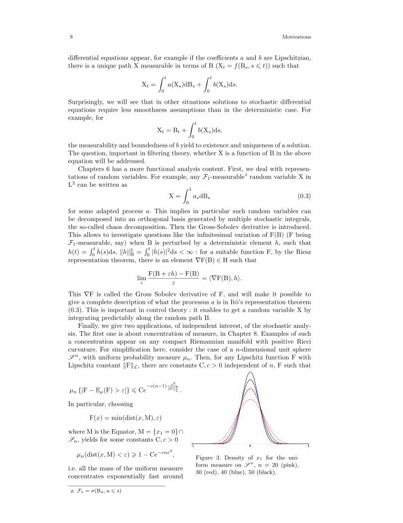
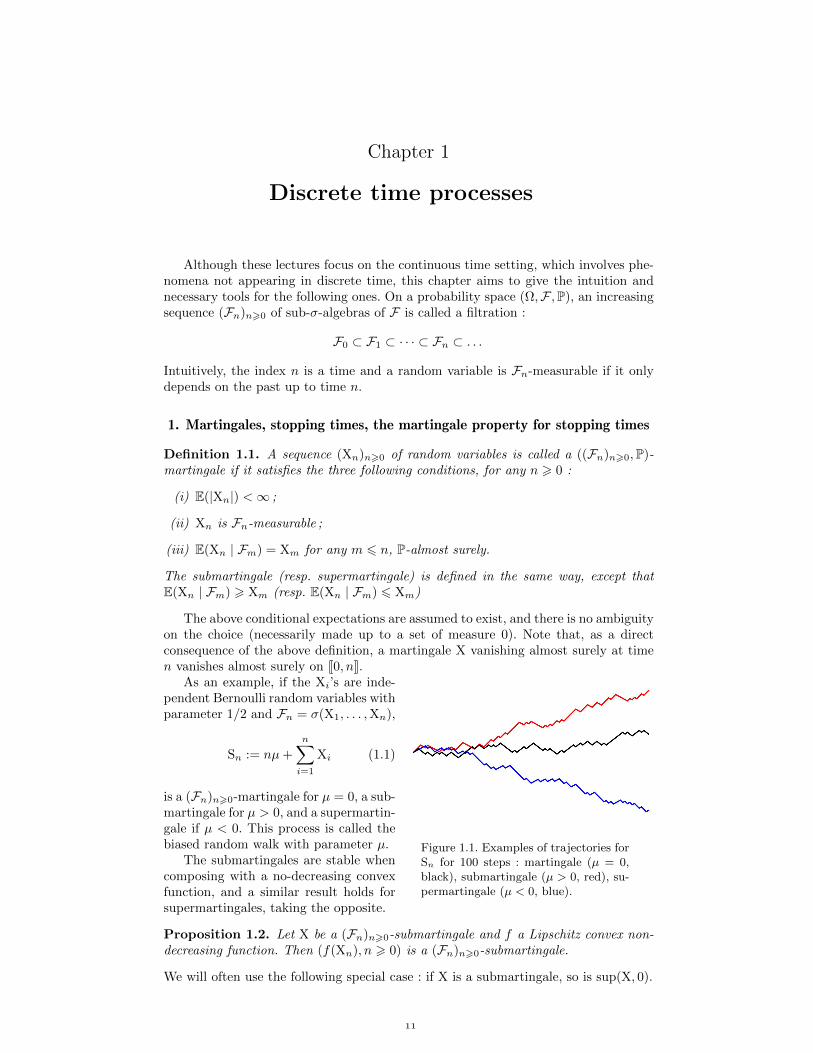
Figure 1.1. Examples of trajectories forSn for 100 steps : martingale (µ = 0,black), submartingale (µ > 0, red), su-permartingale (µ < 0, blue).
As an example, if the Xi’s are inde-pendent Bernoulli random variables withparameter 1/2 and Fn = σ(X1, . . . ,Xn),
Sn := nµ+
n∑i=1
Xi (1.1)
is a (Fn)n>0-martingale for µ = 0, a sub-martingale for µ > 0, and a supermartin-gale if µ < 0. This process is called thebiased random walk with parameter µ.
The submartingales are stable whencomposing with a no-decreasing convexfunction, and a similar result holds forsupermartingales, taking the opposite.
Proposition 1.2. Let X be a (Fn)n>0-submartingale and f a Lipschitz convex non-decreasing function. Then (f(Xn), n > 0) is a (Fn)n>0-submartingale.
We will often use the following special case : if X is a submartingale, so is sup(X, 0).
Discrete time processes
Proof. The Lipschitz hypothesis is just a condition ensuring that f(Xn) is integrable.Now, for n > m, by Jensen’s inequality
E (f(Xn) | Fm) > f (E(Xn | Fm)) .
As E(Xn | Fm) > Xm and f is non-decreasing, this is greater than f(Xm).
Now, consider a specific class of random times adapted to the filtration : theirvalues are determined in view of the past.
Definition 1.3. A function T : Ω→ N ∪ +∞ is a stopping time if T 6 n ∈ Fnfor any n > 0.
An example of stopping time is Ta = infn > 0 | Sn > a, the time when theprocess (1.1) reaches the level a ∈ R.
The definitions prove that the set
FT := A ∈ F | ∀n ∈ N,A ∩ T 6 n ∈ Fn
is a σ-algebra. Intuitively, FT is the information available at time T. Other straight-forward properties are (i) if S 6 T, FS ⊂ FT and (ii) T and XT1T<∞ are FT-measurable.
Proposition 1.4. Let X be a (Fn)n>0-submartingale and (Hn, n > 0) be a boundednonnegative process, with Hn ∈ Fn−1 for n > 1. Then the process Y defined by Y0 = 0and Yn = Yn−1 + Hn(Xn −Xn−1) is a (Fn)n>0-submartingale. In particular, if T isa stopping time, (Xn∧T, n > 0) is a submartingale.
Proof. For the first statement, note that when n > m
E(Yn | Fm) = E(Yn−1 + Hn(Xn −Xn−1) | Fm)
= E(Yn−1 + Hn E(Xn −Xn−1 | Fn−1) | Fm) > E(Yn−1 | Fm).
By an immediate induction, this implies E(Yn | Fm) > Ym. The second statementfollows when choosing Hn = 1n6T, which is Fn−1-measurable by definition of astopping time.
Note that the above result implies that a martingale frozen at a stopping time isstill a martingale.
A natural question is whether the martingale property E(Xn | Fm) = Xm remainswhen m, n are random times. The answer is yes for bounded, ordered stopping times,as shown by the following theorem. To prove it, we first note that if T 6 c is a stoppingtime, then E(XT) = E(X0). Indeed, as T = n ∈ Fn,
E(XT) =
c∑n=1
E(Xn1T=n) =
c∑n=1
E (E(Xc | Fn)1T=n)
=
c∑n=1
E (E(Xc1T=n | Fn)) = E(Xc) = E(X0).
Theorem 1.5 (Doob’s first sampling or stopping theorem). Let (Xn)n>0 be a mar-tingale, and T, S two stopping times such that S 6 T 6 c for some constant c > 0.Then almost surely
E(XT | FS) = XS.
. Example : let T is the first sunny day of the year in Paris, A the event my hibernation has beenlonger than 60 days this year, and B the event at some time in History, Mars is aligned with Jupiterand Saturn. Then, assuming one does not hibernate on sunny days, A ∈ FT and B 6∈ FT. Note that,when replacing Paris with London in the above example, remarkably B ∈ FT.
Discrete time processes
Proof. First, XT 6∑ci=0 |Xi| is clearly integrable and XS is FS measurable, so from
the definition of the conditional expectation we need to check that for any FS mea-surable bounded random variable Z,
E(XTZ) = E(XSZ).
The random variable Z can be chosen of the form 1A where A ∈ FS (by approxima-ting nonnegative random variables by linear combinations of such indicators, and asubstraction gives the result for any bounded Z).
Now, define U as the random time S if ω ∈ A and T if ω 6∈ A. Then U is astopping time, bounded by c, so E(XU) = X0 = E(XT). A simplification, writingXU = XS1A + XT1Ac yields the expected result E(XT1A) = E(XS1A).
This theorem has an immediate equivalent form for submartingales and supermar-tingales evaluated on bounded stopping times. Moreover, note that this boundednessassumption is essential : if S is the random walk (1.1) with parameter µ = 0, andT = infn > 0 | Sn = 1, the (false) equality E(ST | F0) = S0 yields 1 = 0.
Finally, the above result gives easy proofs of not being a stopping time. As anexample, let m > 1 and T = supn ∈ J0,mK | Sn = supJ0,10K Si. The (false) equality
E(ST | F0) = S0 would give E(ST) = 0, obviously false as E(ST) > P(S1 = 1) = 1/2.Hence T is not a stopping time.
2. Inequalities : Lp norms in terms of final values, number of jumps.
Both theorems below are stated for nonnegative submartingale. By by replacing Xby X+ = sup(X, 0) – a submartingale from Proposition 1.2 – they also give estimatesfor general submartingales.
Theorem 1.6 (Doob’s maximal inequality). Let (Xn)n>0 be a non-negative submar-tingale, and X∗n = supJ0,nK Xi. Then for any λ > 0
P(X∗n > λ) 6E(Xn)
λ.
Proof. Hence for any bounded stopping time T 6 n, E(XT) 6 E(Xn).Take T = inf(n, infk | Xk > λ) :
P(X∗n > λ) = P(XT > λ) 61
λE(XT) 6
1
λE(Xn),
which is the expected result.
Theorem 1.7 (Doob’s inequality). Let (Xn)n>0 be a non-negative submartingale.Then for any p > 1
E ((X∗n)p) 6
(p
p− 1
)pE (Xp
n) ,
may the right member be infinite.
Proof. Note that the proof of Doob’s maximal inequality yields slightly more thanstated :
λP(X∗n > λ) 6 E(Xn1X∗n>λ).
Indeed, still writing T = inf(n, infk | Xk > λ), as 1X∗n>λ is FT-measurable andT 6 n,
E(Xn1X∗n>λ) > E(XT1X∗n>λ) > E(λ1XT>λ1X∗n>λ) = λP(XT > λ).
Discrete time processes
Hence we only need to prove that for nonnegative random variables X and Y, if forany λ > 0
λP(Y > λ) 6 E(X1Y>λ), (1.2)
then E(Yp) 6(
pp−1
)pE(Xp). First note that, as yp =
∫ y0pλp−1dλ, E(Yp) =∫∞
0pλp−1P(Y > λ)dλ. This yields, using successively the hypothesis and Holder’s
inequality (we define q by 1/p+ 1/q = 1),
E(Yp) =
∫ ∞0
pλp−1P(Y > λ)dλ 6∫ ∞
0
pλp−2 E(X1Y>λ)dλ
= E
(X
∫ Y
0
pλp−2dλ
)= q E(XYp−1) 6 q‖X‖Lp‖Yp−1‖Lq .
If E(Yp) < ∞, the inequality E(Yp) 6 q‖X‖Lp‖Yp−1‖Lq can be simplified and givesthe required result. If E(Yp) = ∞, for any m > 0 define Tm = infk > 0 | |Xk| >m ∧ n. Then by using the previous result for the submartingale (Xn∧Tm)n>0, weobtain
‖ sup06k6n
Xk∧Tm‖pLp 6
(p
p− 1
)p‖Xn‖pLp .
By monotone convergence, taking m→∞ allows to conclude.
Remark. For p = 1, a similar inequality holds :
E (X∗n) 6e
e− 1
(1 + E(|Xn| log+ |Xn|)
),
Both of Doob’s inequalities above will be important in the next chapters as itallows to control uniform convergence of martingales from their distribution at agiven time.
Theorem 1.8 (Doob’s jumps inequality). Let (Xn)n>0 be a submartingale and a < b.Let Un be the number of jumps from a to b before time n. More precisely, define byinduction T0 = 0, Sj+1 = infk > Tj | Xk 6 a and Tj+1 = infk > Sj+1 | Xk > b.Then Un = supj | Tj 6 n.
Then
E(Un) 61
b− aE ((Xn − a)+) .
Proof. Let Yn := (Xn − a)+. By definition, YTi −YSi > b− a for the above stoppingtimes Ti, Si smaller than n. Consequently,
Yn = YS1∧n +∑i>1
(YTi∧n −YSi∧n) +∑i>1
(YSi+1∧n −YTi∧n)
> (b− a)Un +∑i>1
(YSi+1∧n −YTi∧n).
Now, as x → (x − a)+ is convex and X is a submartingale, so is Y, from Propo-sition 1.2. Consequently, as Si+1 ∧ n > Ti ∧ n are increasing bounded stoppingtimes, E(YSi+1∧n) > E(YTi∧n), so taking expectations in the previous inequalityyields E(Yn) > (b− a)E(Un), the expected result.
3. Convergence of martingales.
Theorem 1.9 (Convergence of submartingales). Let Xn be a submartingale suchthat supn E ((Xn)+) < ∞. Then Xn converges almost surely to some X ∈ R andX ∈ L1(Ω,F ,P).
Discrete time processes
Proof. Given any a < b, let Un(a, b) be the number of jumps from a to b before time n,like in Theorem 1.8. By monotone convergence, E(U∞(a, b)) = limn→∞ E(Un(a, b)).But E(Un(a, b)) is uniformly bounded :
E(Un(a, b)) 61
b− aE((Xn − a)+) 6
1
b− a(E(Xn)+ + a) .
Consequently, E(U∞(a, b)) < ∞, so U∞(a, b) < ∞ almost surely. From the inclusionof events
∩a<b,a,b∈QU∞(a, b) <∞ ⊂ Xn convergeswe conclude that Xn converges almost surely. The limit X eventually can be ±∞, butthis is not the case. Indeed, note that |x| = 2x+ − x, so
E(|Xn|) = 2E((Xn)+)− E(Xn) 6 2E((Xn)+)− E(X0)
because E(Xn) > E(X0) (X is a submartingale). Hence, from the hypothesis, E(|Xn|)is uniformly bounded, and using Fatou’s lemma
E(|X|) = E(limn|Xn|) 6 lim inf E(|Xn|) <∞.
We proved that |X| is integrable, so X ∈ R almost surely.
For the following result, the notion of uniformly integrable family of random va-riables is required : this is a set Xnn>0 of elements in L1(Ω,F ,P) such that
limλ→∞
supn
E(|Xn|1|Xn|>λ) = 0.
A (Ω,F ,P)-martingale X is said to be uniformly integrable if Xnn>0 is uniformlyintegrable. There are many criteria to prove uniform integrability. For example if, forsome p > 1, supn E(|Xn|p) < ∞, the family is uniformly integrable. If there is anintegrable Y such that, for any n, Xn 6 Y, then the family Xnn>0 is integrable.
A straightforward reasoning yields that if X is integrable, Xn := E(X | Fn) is auniformly integrable martingale. The following result shows that the converse is true.
Theorem 1.10 (Convergence of martingales). Let Xn be a uniformly integrable mar-tingale. Then Xn converges almost surely and in L1(Ω,F ,P) to some integrable X ∈ Rand Xn = E (X | Fn) for any n > 0.
Proof. As the family is uniformly integrable, for some ε > 0 there is a λ > 0 suchthat supn E(|Xn|1|Xn|>λ) < ε. Hence
E((Xn)+) 6 E(|Xn|) = E(|Xn|1|Xn|>λ) + E(|Xn|1|Xn|6λ) 6 ε+ λ,
so supn E((Xn)+) <∞ and the convergence of submartingales, Theorem 1.9, impliesthat (Xn)n>0 converges almost surely to some X ∈ L1(Ω,F ,P).
Now, take any ε > 0 and note, for any λ > 0,
fλ(x) = x1|x|6λ + λ1x>λ − λ1x<−λ.
The uniform integrability implies that there is a sufficiently large λ > 0 such that
E(|Xn − fλ(Xn)|) < ε. (1.3)
Moreover, as X ∈ L1(Ω,F ,P), dominated convergence implies that, for sufficientlylarge λ,
E(|X− fλ(X)|) < ε. (1.4)
Finally, Xn → X a.s. so fλ(Xn) → fλ(X) a.s. by continuity of fλ. This implies bydominated convergence that given λ, for sufficiently large n
E(|fλ(X)− fλ(Xn)|) < ε. (1.5)
Discrete time processes
Equations (1.3), (1.4) and (1.5) together prove that Xn converges to X in L1.Our last task is proving that Xn = E(X | Fn). As usual, taking some A ∈ Fn, we
need to prove thatE(Xn1A) = E(X1A). (1.6)
For any m > n, as Xn = E(Xm | Fn), E(Xn1A) = E(Xm1A). Consequently,
|E(Xn1A)−E(X1A)| 6 |E(Xn1A)−E(Xm1A)|+|E(Xm1A)−E(X1A)| 6 E(|Xm−X|).
As Xm → X in L1, this converges to 0 as m→∞, which proves (1.6).
Theorem 1.11 (Doob’s optional sampling or stopping theorem). Let (Xn)n>0 be auniformly integrable martingale, and T, S two stopping times such that S 6 T. Thenalmost surely
E(XT | FS) = XS.
Proof. We first prove the result when T = ∞. We know, by Theorem 1.10, that Xn
converges almost surely and in L1 to some X ∈ L1. Then, note that for any n ∈ N,
E(X | FS)1S=n = E(X | Fn)1S=n. (1.7)
To prove the above identity, note that both terms are Fn-measurable and that, forany A ∈ Fn,∫
A∪S=nE(X | Fn)dP =
∫A∪S=n
XdP =
∫A∪S=n
E(X | FS)dP
because A ∪ S = n is both in Fn and FS. Now, using Theorem 1.10 and (1.7),
XS =∑n
Xn1S=n =∑n
E(X | Fn)1S=n =∑n
E(X | FS)1S=n = E(X | FS),
where the summation over n includes the case n = ∞, corresponding to XS = X, incase S is ∞ with positive probability. This gives the expected result when T = ∞,and the conditioning
XS = E(X | FS) = E(E(X | FT) | FS) = E(XT | FS)
yields the general case.
We end this chapter with a convergence result about processes indexed by −N,this will be useful when extending Theorem 1.11 to the continuous setting. An inversemartingale is a sequence of random variables (X−n, n > 0) in L1 such that for m >n > 0
E(X−n | F−m) = X−m
almost surely, where F−m ⊂ F−n : (F−n, n > 0) can be thought of as a filtrationindexed by negative times.
Theorem 1.12. Let (X−n, n > 0) be an inverse martingale for the filtration(F−n, n > 0). Then, as n→∞, Xn converges a.s. and in L1 to some X ∈ L1.
Proof. The proof is very similar to the one of Theorems 1.9 and 1.10. First, for anya < b the number of jumps from a to b is almost surely finite from the Doob’s jumpsinequality Theorem 1.8 :
E(U(a, b)) = limn→∞
E(Un(a, b)) 61
b− aE((X0 − a)+) <∞,
Discrete time processes
where Un(a, b) is the number of jumps between times −n and 0. As a consequence,X−n converges almost surely to some X, eventually equal to ±∞. As x+ is convexand nondecreasing, Fatou’s lemma and Proposition 1.2 yield
E(X+) 6 lim infn→∞
E((X−n)+) 6 E((X0)+) <∞.
In the same way one can consider −X, giving X ∈ L1, so in particular X is finite. Thelast step consists in proving the convergence in L1. Copying the proof of Theorem 1.10,we just need to know that the family of random variables (X−n, n > 0) is uniformlyintegrable. This is automatic because X−n = E(X0 | F−n).
. The only difference with the proof of Theorem 1.9 is that here the condition supn E((X−n)+) <∞is automatically true thanks to the negative indexation

Chapter 2
Brownian motion
After reminding some elementary facts about Gaussian random variables, we willbe ready for constructing one specific random trajectory, the Brownian motion, andstudy its basic properties. At the end of the chapter, it is shown to be universal asa continuous limit of random walks. In the next two chapters, it will be shown to beuniversal amongst continuous martingales.
1. Gaussian vectors
This section is a reminder about properties of Gaussian vectors useful in thefollowing. First, a random variable X is said to be Gaussian with expectation µ andvariance σ2 (X ∼ N (µ, σ)) if its law has density
1√2πσ2
e−(x−µ)2
2σ2
with respect to the Lebesgue measure. By convention, the Dirac measure δµ is
Gaussian with distribution N (µ, 0). Hence, if X ∼ N (µ, σ2), Xlaw= µ + σY where
Y ∼ N (0, 1).
Theorem 2.1. If X ∼ N (µ, σ2), for any t ∈ R
E(eitX) = eitµ− (σt)2
2
If X1 and X2 are independent Gaussian random variables (X1 ∼ N (µ1, σ21),X2 ∼
N (µ2, σ22)), X1 + X2 is Gaussian with expectation µ1 + µ2 and variance σ2
1 + σ22.
Proof. To prove the form of the characteristic function, as Xlaw= µ + σY where Y ∼
N (0, 1), we only need to prove that
f(t) := E(eitY) = e−t2
2 .
Derivation into the integral sign is clearly allowed, and a subsequent integration byparts yields
f ′(t) =1√2π
∫R
ixeitxe−x2
2 = −tf(t).
As f(0) = 1, the unique solution is f(t) = e−t2
2 .Now, for X1 and X2 as in the hypothesis, by independence
E(eit(X1+X2)
)= E
(eitX1
)E(eitX2
)= eit(µ1+µ2)− (σ21+σ22)t2
2 .
As the characteristic function uniquely determines the law, this means that X1 + X2
is Gaussian with mean µ1 + µ2 and variance σ21 + σ2
2 .
The rigidity of the family of Gaussian measures implies that it is stable by conver-gence in law, and that convergence in probability implies Lp convergence.
Theorem 2.2. Let Xn ∼ N (λn, σ2n).
Brownian motion
(i) If Xnlaw−→ X, then λn (resp. σ2
n) converges to some λ ∈ R (resp. σ2 ∈ R+) andX ∼ N (λ, σ2).
(ii) If XnP−→ X then, for any p > 1, Xn
Lp−→ X.
Proof. Concerning (i), we know that the convergence in law implies the uniformconvergence of characteristic functions on compact sets, i.e.
E(eitXn
)= eitµn−
σ2nt2
2 −→n→∞
E(eitX
).
Taking the modulus, σ2n converges to some σ2 ∈ R+ (σ2 = ∞ is not possible as
E(eitX) would be discontinuous, 1t=0). If (µn, n > 0) is bounded, this implies that
µn → µ ∈ R because for any accumulation points µ, µ′, for any t, eitµ = eitµ′ , soµ = µ′, and by convergence of the characteristic functions Xn converges in law toGaussian N (µ, σ2).
The unbounded case is impossible : if for example a subsequence µnk →∞, thenas the variables are Gaussian and σ2
n is bounded P(Xnk > λ) → 1 for any λ, so byweak convergence P(X > λ) = 1, a contradiction when λ is large enough.
For (ii), first note that we just proved that µn and σ2n are bounded. Hence we have
supn E(|Xn|2p) <∞ for any p > 0. By Fatou’s lemma, as Xmk converges almost surelyto X along a subsequence, this implies that E(|X|2p) <∞, and therefore supn E(|Xn−X|2p) <∞. Hence the sequence (Xn −X, n > 0) is bounded in L2 and converges to 0in probability, hence it converges to 0 in L1, as expected.
We now come to a multidimensional natural generalization : a random variable Xwith values in Rd is called a Gaussian vector if any linear combination of the coordi-nates is a Gaussian random variable : for any u ∈ Rd, u ·X is normally distributed.
For example, if X1, . . . ,Xd are independent Gaussians, X = (X1, . . . ,Xd) is aGaussian vector. Under the same hypothesis, if M is a d′ × d, MX is still a Gaussian
vector with values in Rd′ . Note that there are vectors with Gaussian entries which arenot Gaussian vectors. For example, if X ∼ N (0, 1) and ε is an independent randomvariable, P(ε = 1) = P(ε = −1) = 1/2, then (X, εX) has Gaussian entries but is not aGaussian vector : the sum of its coordinates has probability 1/2 to be 0.
Theorem 2.3. Let X be a Gaussian vector. Then its entries are independent if andonly if its covariance matrix (cov(Xi,Xj))16i,j6d is diagonal.
Proof. If the entries are independent, the covariance matrix is obviously diagonal.Reciprocally, if the matrix is diagonal, for any u ∈ Rd
E(u ·X) =∑
ui E(Xi)
var(u ·X) =∑j,k
ujuk cov(Xi,Xj) =∑j
u2j var(Xj)
Hence the Gaussian random variable u ·X has characteristic function
E(eiu·X) = eiE(u·X)− var(u·X)2 =
d∏k=1
eiuk E(Xk)− var(Xk)
2 =
n∏k=1
E(eiukXk).
As a consequence of this splitting of the characteristic function, the Xk’s are inde-pendent.
Finally, in this section we want to give a useful estimate of the queuing distributionof Gaussian random variables.
Lemma 2.4. Let X ∼ N (0, 1). Then, as λ→∞,
P(X > λ) ∼ 1
λ√
2πe−
λ2
2
Brownian motion
Proof. By integration by parts,
P(X > λ) =1√2π
∫ ∞λ
−1
x(−x)e−
x2
2 =1
λ√
2πe−
λ2
2 − 1√2π
∫ ∞λ
e−x2/2
x2dx.
Obviously,
1√2π
∫ ∞λ
e−x2/2
x2dx 6
1
λ2√
2π
∫ ∞λ
e−x2/2dx = o (P(X > λ)) ,
concluding the proof.
2. Existence of Brownian motion
Definition 2.5. (Xt, t > 0) is a Gaussian process if for any (t1, . . . , tn) ∈ Rn+,(Xt1 , . . . ,Xtn) is a Gaussian vector.
Definition 2.6. A process B = (Bt, t > 0) is called a Brownian motion if :
(i) it is a Gaussian process ;
(ii) it is centered : for any t > 0, E(Bt) = 0 ;
(iii) for any (s, t) ∈ R2+, E(BsBt) = s ∧ t ;
(iv) it is almost surely continuous.
Note that this definition implies B0 = 0 almost surely. One refer sometimes tothis process B as a standard Brownian motion, in contrast to x+ B which is called aBrownian motion starting at x. Some variants of the definition also englobe the finitehorizon possibility, refering to a Brownian motion on [0,T].
The above definition is equivalent to another one, with independence of the incre-ments.
Proposition 2.7. The process (Bt, t > 0) is a Brownian motion if and only if
(a) B0 = 0 almost surely ;
(b) for any n > 2, 0 6 t1 6 · · · 6 tn, (Bt1 ,Bt2 − Bt1 , . . . ,Btn − Btn−1) is a Gaussianvector with independent coordinates.
(c) for any (s, t) ∈ R2+, Bt − Bs ∼ N (0, |t− s|) ;
(d) it is almost surely continuous.
Proof. Let us first prove that (i), (ii), (iii) implies (a), (b), (c). By (iii), B0 = 0 a.s.which is (a). Moreover, X = (Bt1 ,Bt2 − Bt1 , . . . ,Btn − Btn−1
) is clearly a Gaussianvector, because by (i), (Bt1 ,Bt2 , . . . ,Btn) is a Gaussian vector. To prove that thecoordinates are independent, we just need to prove that the covariance matrix isdiagonal. This is a direct calculation, using (iii) : for t1 6 t2 6 t3 6 t4,
cov(Bt4−Bt3 ,Bt2−Bt1) = E((Bt4−Bt3)(Bt2−Bt1)) = t4∧t2−t4∧t1−t3∧t2+t3∧t1 = 0.
By (i), Bt − Bs is a Gaussian random variable, with expectation E(Bt) − E(Bs) = 0by (ii) and variance
E((Bt − Bs)2) = E(B2
t ) + E(B2s)− 2E(BtBs) = ts− 2s ∧ t = |t− s|,
by (iii), proving (c).Now, assume points (a), (b), (c). For any t1 6 · · · 6 tn, as (Bt1 ,Bt2−Bt1 , . . . ,Btn−
Btn−1) is Gaussian by (b), so is (Bt1 ,Bt2 , . . . ,Btn), because (x1, . . . , xn) 7→ (x1, x2 −
Brownian motion
x1, . . . , xn − xn−1) is invertible. This proves (i). Point (ii) follows from Bt ∼ N (0, t),by (a) and (c). Finally, using the independence of the increments in (b), the previouslyproved fact that B is centered, and the variance of B given by (c), for t > s
E(BtBs) = E(B2s) + E((Bt − Bs)Bs) = E(B2
s) + E((Bt − Bs)Bs) = s = s ∧ t,
which proves (iii).
In the following, we give two constructions of Brownian motion. The first one, byPaul Levy, is intuitive and proceeds by almost sure uniform convergence of properlychosen piecewise affine gaussian processes. Then a more functional analytic proof willbe discussed, originating in the work of Wiener and substantially generalized by Itoand Nisio. Both proofs exhibit a Brownian motion on [0, 1], extending to the existencein R+ by simple juxtaposition of independent ones on [0, 1].
Theorem 2.8. The Brownian motion exists.
Proof. We proceed by induction to construct piecewise affine Gaussian processesconverging uniformly. First, take a Gaussian random variable N0,0 ∼ N (0, 1), anddefine f0(t) = N0,0t, 0 6 t 6 1. This is a Gaussian process with the same distributionas Brownian motion at time 1, but not on (0, 1). To avoid this problem, define anotherN (0, 1) random variable N1,1 and the Gaussian process f1, piecewise affine, conti-
nuous, such that f1 and f0 coincide on 0 and 1, but f1(1/2) = f0(1/2) + 12N1,1. Now
the process f1 has the expected covariance function on the set of points 0, 1/2, 1. Weproceed in the same way on further intervals, defining for any n > 1 the continuousfunction fn, affine on [(k − 1)/2n, k/2n] for any k ∈ J1, 2nK, by
fn(
2`2n
)= fn−1
(`
2n−1
)fn(
2`−12n
)= fn−1
(2`−12n−1
)+ 2−
n+12 N`,n
,
where the Nn,`, n > 0, 1 6 ` 6 2n−1 are independent standard Gaussians. Thenan immediate induction proves that for any n > 1, (fn(t), 0 6 t 6 1) is a centeredGaussian process, and with covariance function
E(fn
(j
2n
)fn
(k
2n
))=
j
2n∧ k
2n, (2.1)
the normalization 2−n+12 in the definition of fn being chosen to get the above appro-
priate covariance.We are now interested in the uniform convergence of fn, n > 0. Let
An = sup[0,1]
|fn − fn−1|(t) > 2−n/4.
As |fn− fn−1| is continuous affine on [(k− 1)/2n, k/2n] for any k ∈ J1, 2nK, and 0 if kis even, its maximal value is obtained at some t ∈ (2`− 1)/2n, 1 6 ` 6 2n−1, hence
P(An) = P
(sup
16`62n−1
|2−n+12 N`,n| > 2−n/4
)
62n−1∑`=1
P(|N`,n| > 2−n/4+n+1
2
)P(An) 6 2c1ne−c22n/2
for some absolute constants c1, c2 > 0, where we used Lemma 2.4. Hence∑n P(An) <
∞, which means by the Borel-Cantelli lemma that almost surely, there is an index
Brownian motion
n0(ω) such that if n > n0(ω) then ‖fn − fn−1‖∞ 6 2−n/4. This implies the almostsure uniform convergence of fn on [0, 1], to a random function called f .
This process is almost surely continuous, as the a.s. uniform limit of continuousfunctions, and this is Gaussian process because the a.s. limit of Gaussian vectors is aGaussian vector, by Theorem 2.2.
Our only remaining point to prove is
E(f(s)f(t)) = s ∧ t. (2.2)
Let `(s)n , `
(t)n be integers such that
`(s)n
2n6 s <
`(s)n + 1
2n,`(t)n
2n6 t <
`(t)n + 1
2n.
From the uniform convergence of fn, the Gaussian vector (fn(`(s)n /2n), fn(`
(t)n /2n))
converges almost surely to (f(s), f(t)), hence in L2 by Theorem 2.2. This implies
E(fn(`(s)n /2n)fn(`(t)n /2n))→ E(f(s)f(t)),
and this first term also obviously converges to s ∧ t by (2.1), proving (2.2).
We note that there is only one Brownian motion : the subsets of type
ω : ω(t1) ∈ A1, . . . , ω(tm) ∈ Am,
where the Am’s are Borel subsets of R, have a unique possible measure given thedefinition of Brownian motion. As they are stable by intersection and generate thesigma algebra F = σ(ω(s), 0 6 s 6 1), by the monotone class theorem there is onlyone measure on F corresponding to a Brownian motion. The Wiener measure, notedW, is the image of the Gaussian product measure (for the Nk’s) on C o([0, 1]) in theabove construction.
For another construction of Brownian motion, we need the following theorem byIto and Nisio [6], where E is a real separable Banach space, with its norm topology,E∗ its dual and B its Borel algebra.
Theorem 2.9. Let (Xi)i>0 be independent E-valued random variables, and Sn =∑n1 Xi, with law µn. Then the following three conditions are equivalent :
(a) Sn converges almost surely ;
(b) Sn converges in probability ;
(c) µn converges for the Prokhorov metric.
Moreover, if the Xi’s have a symmetric distribution (Xilaw= −Xi), then each of the
above conditions is equivalent to any of the following ones :
(d) µn is uniformly tight ;
(e) there is a E-valued S such that for any z ∈ E∗, 〈z,Sn〉P−→ 〈z,S〉 ;
(f) there is a measure µ on E such that for any z ∈ E∗, E(ei〈z,Sn〉
)→∫ei〈z,x〉dµ(x).
. The Prokhoov distance between two measures µ and ν is
π(µ, ν) = infε > 0 : ∀A ∈ B, µ(A)− ν(Aε) 6 ε, µ(Aε)− ν(A) 6 ε,where Aε is the set of points within distance at most ε to A.
Brownian motion
In finite dimension, the symmetry condition for points (d), (e), (f) is not necessary,but it is essential in infinite dimension, as shown by the following example : if (ei)i>1
is an orthonormal basis of a Hilbert space, and X1(ω) = e1, Xn(ω) = en − en−1 forn > 2, then Sn(ω) = en, so 〈z,Sn〉 → 0 but Sn does not converge almost surely.
The application of the previous general result to Brownian motion is for E =(C ([0, 1]), ‖‖∞), the space of continuous functions on [0, 1] endowed with the supnorm.
Theorem 2.10. Let (ϕn)n>1 be an orthonormal basis of L2([0, 1]), composed of conti-nuous functions, and (Nk)k>1 a sequence of independent standard normal variables.Then
Sn(t) =
n∑k=1
Nk
∫ t
0
ϕk(u)du
converges uniformly in t ∈ [0, 1] as n→∞. The limit S is a Brownian motion.
Proof. Elements in E∗ can be identified with bounded signed finitely additive mea-sures on [0, 1] that are absolutely continuous with respect to the Lebesgue measureon [0,1], see [4].
Let dz be such an element : we first prove point (f) in Theorem 2.9, by writing
E(ei〈z,Sn〉) =
n∏k=1
E(eiNk〈z,
∫ .0ϕk〉)
=
n∏k=1
e−12 |〈z,
∫ .0ϕk〉|2
= e−12
∑nk=1(
∫ 10
dz(u)∫ u0ϕk(s)ds)
2
= e−12
∑nk=1(
∫ 10ϕk(s)dsz([s,1]))
2
−→n→∞
e−12
∫ 10
dsz([s,1])2 = e−12
∫[0,1]2
(s∧t)dz(s)dz(t),
where we used the orthonomality of the ϕk’s between the second and third lines.Now, if B is a Brownian motion, as proved by approximations by Riemann sums,
〈z,B〉 is a Gaussian random variable with variance∫
[0,1]2(s ∧ t)dz(s)dz(t). Conse-
quently, E(ei〈z,Sn〉) converges to∫ei〈z,x〉dW(x) where W is the Wiener measure. As
Xk = (Nk
∫ t0ϕk(u)du, 0 6 t 6 1) is symmetric, by Theorem 2.9 Sn converges almost
surely uniformly on [0, 1].The limit is a Brownian motion : all the characteristic properties of B (independent
Gaussian increments) are proved by choosing z =∑mk=1 δtk in the above calculation.
3. Invariance properties
One of the useful features of Brownian motion is the invariance of the Wienermeasure under many transformations, i.e. symmetry, time reversal, time inversionand scaling.
Theorem 2.11. Let (Bt, t > 0) be a Brownian motion. Then the following processesare Brownian motions :
(i) Xt = −Bt, t > 0 ;
(ii) Xt = BT − BT−t, 0 6 t 6 T ;
(iii) Xt = tB1/t if t > 0 and 0 it t = 0 ;
(iv) Xt = 1√λ
Bλt, t > 0, for some given parameter λ > 0.
Proof. It is an easy task to prove that all of these processes are centered Gaussianprocesses with covariance function E(XsXt) = s ∧ t. The only problem consists inproving the almost sure continuity of X at 0 in the case (iii).
Brownian motion
As (Bs, s > 0) has the same law as (sB1/s, s > 0), for any ε > 0
P(∩n ∪t∈Q∩(0,1/n] |tB1/t| > ε
)= P
(∩n ∪t∈Q∩(0,1/n] |Bt| > ε
).
This last term is 0 because almost surely B0 = 0 and B is continuous. Hence sB1/s → 0along positive rational numbers, hence along R+ by continuity.
Note that as Bt → 0 almost surely as t → 0+, point (iii) implies that Btt → 0 as
t→∞. One can directly show that
Mt := eBt− t2
has constant expectation, and thanks to the above property it converges almost surelyto 0 : this is an example of almost sure convergence but no convergence in L1.
4. Regularity of trajectories
In this section, we are interested in the Holder exponent of the trajectories of B,i.e. the values of α such that there is almost surely a constant cα(ω) such that, forany s and t in [0, 1],
|Bt − Bs| 6 cα(ω)|t− s|α.This set of possible values for α is of type [0, α0] or [0, α0), and in the next sectionwe will give the precise value of α0.
First, before giving the important criterium by Kolmogorov for Holder-continuity,we need to introduce the following notions.
Definition 2.12. Let (Xt)t∈I and (Xt)t∈I be two processes.
(i) X is called a version of X if, for any t ∈ I, P(Xt = Xt) = 1 ;
(ii) X and X are called indistinguishable if P(∀t ∈ I,Xt = Xt) = 1.
Is X and X are indistinguishable, each one is a version of the other. The converse
is false, as shown by X(t) = 0, 0 6 t 6 1 and Xt = 0 on [0, 1] except on U, uniform
on [0, 1], where X is 1. Then on a given t both processes are almost surely equal butalmost surely, they differ somewhere along the trajectory.
Note that if I is countable, or if X and X are almost surely continuous, then beinga version of the other implies the indistinguishability.
Theorem 2.13. Let I be a compact interval and X a process on I. We suppose thatthere exist p, ε and c positive numbers such that for any s, t in I
E (|Xs −Xt|p) 6 c|t− s|1+ε.
Then there exists a version X of X whose trajectories are Holderian with index α forany α ∈ [0, ε/p) : almost surely, there is cα(ω) > 0 such that for any s, t in I
|Xt − Xs| 6 cα(ω)|t− s|α.
Proof. If α = 0 the result is obvious by compactness of the support, so we supposeα ∈ (0, ε/p) in the following. We can suppose I = [0, 1], and we will first show theHolder property for X on the set D of dyadic numbers, i.e. of type
m∑k=1
εk2k
for some m ∈ N∗, and εk = 0 or 1. We want to prove that for α ∈ (0, ε/p),
sups,t∈D,s 6=t
|Xt −Xs||t− s|α
<∞.
Brownian motion
Let us first prove that
dα = supn>0
sup16i62n
|X i2n−X i−1
2n|
|1/2n|α<∞ (2.3)
almost surely. For this, let A(n)i = |X i
2n−X i−1
2n| > 2nα. As
P(|Xt −Xs| > a) 6 a−p E(|Xt −Xs|p) 6 ca−p|t− s|1+ε,
we have P(A(n)i ) 6 c2(pα−1−ε)n. As pα− ε < 0, this yields∑
n>0
P(∪2n
i=1A(n)i
)<∞,
so by the Borel Cantelli lemma dα <∞ almost surely.We now want to extend the result to dyadic numbers. For this, for given s < t in
D , let q be the smallest integer such that 2−q < t− s. We can writes = k2−q −
∑`i=1 εi2
−q−i
t = k2−q +∑mi=1 ε
′i2−q−i
for some integers k, ` and m, and the εi’s, ε′i’s being 0 or 1. Define for j ∈ J0, `K and
0 ∈ J1,mK, sj = k2−q −
∑ji=1 εi2
−q−i
tk = k2−q +∑ki=1 ε
′i2−q−i
Then, using (2.3) between successive sj ’s and tj ’s
|Xt −Xs| 6∑j=1
|Xsj −Xsj−1 |+m∑k=1
|Xtk −Xtk−1|
6 dα
∑j=1
2−(q+j)α +
m∑k=1
2−(q+k)α
6 2dα
1
1− 2−α2−pα
|Xt −Xs| 6 cα|t− s|α,
proving that X is Holderian with exponent α on dyadic numbers. Define X as 0 ifdα(ω) = ∞ (event with measure 0) and the continuous extension of X from D to
[0, 1] otherwise, which exists and is unique thanks to the previous results : X is stillHolderian for the exponent α, and we just need to prove that it is a version of X.For a given t ∈ [0, 1], consider a sequence (sn)n>0 of diadic numbers converging to t.From the hypothesis, Xsn converges to Xt in Lp, hence in probability, hence almost
surely along a subsequence. Moreover, along that subsequence, Xsn converges to Xt
by definition of X. Consequently, almost surely both limits coincide, i.e. P(Xt = Xt) =1.
Corollary 2.14. Let B = (Bt, 0 6 t 6 1) be a Browian motion. Then B is almostsurely Holderian with exponent α for any α ∈ [0, 1/2).
Proof. For any s and t,, if X ∼ N (0, 1),
E (|Bt − Bs|p) = E (|X|p) |t− s|p/2.
For p > 2, if ε = p2 − 1 in Theorem 2.13, we see that B has a Holderian version with
exponent α for any α ∈[0, 1
2 −1p
). As B and its version are almost surely continuous,
they are indistinguishable and taking p→∞ previously proves that B is almost surelyHolderian for any exponent α ∈ [0, 1/2).
Brownian motion
Section 6 will prove that the set of values of α for which a Brownian trajectory isalmost surely Holderian is exactly [0, 1/2).
5. Markov properties
Let Ft = σ(Bs, 0 6 s 6 t), i.e. Ft is the smallest σ-algebra in Ω such that allBs : Ω→ R, 0 6 s 6 t, are measurable.
Then the weak Markov property states that, writing Bt = Bt+s − Bs, B is aBrownian motion independent of Fs. Being a Brownian motion is a straightforwardconsequence of the definition. To get the independence property, by the monotone classTheorem, it is sufficient to prove that for 0 6 t1 < · · · < tm, 0 6 s1 < · · · < sm 6 s,
the vectors b = (Bt1 , . . . , Btn) and b = (Bs1 , . . . ,Bsm) are independent. Note that
cov(Btj ,Bsk) = E((Bs+tj − Bs)Bsk) = E(Bs+tj − Bs)E(Bsk) = 0,
thanks to the independence of increments of the Brownian motion and sk 6 s 6 s+tj .
Hence for any λ = (λ1, . . . , λm) and µ = (µ1, . . . , µn), the Gaussian vector (λ · b, µ · b)has a diagonal covariance matrix, and by Theorem 2.3 λ · b and µ · b are independent.
This being true for any λ and µ, b and b are independent, as expected.The above result can be extended to a σ-algebra potentially bigger than Fs, namely
F+s = ∩t>sFt.
Theorem 2.15 (Weak Markov property). Let Bt = Bt+s−Bs. Then B is a Brownianmotion independent of F+
s
Proof. Proving the independence property requires some work. By the monotone classTheorem, a sufficient condition is that for any A ∈ F+
s , n > 0, 0 6 t1 < · · · < tn, andF : Rn → R bounded and continuous,
E(
F(Bt1 , . . . , Btn)1A
)= E
(F(Bt1 , . . . , Btn)
)E (1A) . (2.4)
For any ε > 0, as (Bt+s+ε − Bs+ε, t > 0) is a Brownian motion independent of Fs+εand A ∈ Fs+ε,
E (F(Bt1+s+ε − Bs+ε, . . . ,Btn+s+ε − Bs+ε)1A)
= E (F(Bt1+s+ε − Bs+ε, . . . ,Btn+s+ε − Bs+ε))E (1A) .
By dominated convergence, ε→ 0 in the above equation yields the result (2.4).
As a consequence of the weak Markov property, the σ-algebra F+0 is trivial : there
is no information in the germ of the Brownian motion.
Theorem 2.16 (Blumenthal’s 0-1 law). For any A ∈ F+0 , P(A) = 0 or P(A) = 1.
Proof. From Theorem 2.15, A is independent of (Bt − B0, t > 0), hence independent
of σ(Bs, s > 0). Moreover, A ∈ F+0 ⊂ σ(Bs, s > 0), hence A is independent of itself :
P(A) = E(1A1A) = E(1A)E(1A) = P(A)2,
so P(A) = 0 or P(A) = 1.
Corollary 2.17.
(i) Let τ1 = inft > 0 : Bt > 0. Then τ1 = 0 almost surely.
(ii) Let τ2 = inft > 0 : Bt = 0. Then τ2 = 0 almost surely.
Brownian motion
(iii) Let τ3 = supt > 0 : Bt = 0. Then τ3 =∞ almost surely.
Proof. First note that
τ1 = 0 = ∩n>1 sup[0,1/n]
Bs > 0 ∈ ∩t>0Ft = F0+,
so, from Theorem 2.16, P(τ1 = 0) = 0 or 1. Moreover, by monotone convergence,
P(τ1 = 0) = limε→0
P(τ1 6 ε) > limε→0
P(Bε > 0) = 1/2,
so P(τ1 = 0) = 1, proving (i). By symmetry, inft > 0 : Bt < 0 = 0 a.s. sopoint (ii) comes from the a.s. continuity of the Brownian path and the intermediatevalue theorem. From Theorem 2.11, (tB1/t, t > 0) is a Brownian motion, so (ii) gives
inft > 0 : tB1/t = 0 = 0 almost surely, i.e. supt > 0 : Bt = 0 = ∞ almost surely,
proving (iii).
We now prove the strong Markov property, i.e. an analogue of Theorem 2.15 wherethe shifted Brownian motion begins from a stopping time. For this, we need to definenotions analogue to what was discussed in the discrete setting, Chapter 1.
Definition 2.18. On a probability space (Ω,F ,P), a filtration (Ft)t>0 is an increasingsequence of sub-σ-algebras of F .
A random variable T : Ω→ R+ ∪ ∞ is called a stopping time with respect to afiltration (Ft)t>0 if, for any t > 0, T 6 t ∈ Ft.
Examples of stopping times with respect to the Brownian filtration include
Ta = inft > 0 : Bt = a.
Indeed, if for example a > 0, Ta 6 t = sup[0,t] Bs > a = sup[0,t]∩Q Bs > a by
continuity of the Brownian path, so Ta 6 t is a countable union of Ft-measurableevents, hence it is in Ft. As we will see thanks to the stopping time theorems, not allF-measurable times are stopping times. As an example, g = supt ∈ [0, 1] : Bt = 0is not a stopping time.
Given a stopping time T, the information available till time T is defined as
FT = A ∈ F : ∀t > 0,A ∩ T 6 t ∈ Ft.
As an exercise, one can prove that this is a σ-algebra, and that T,BT1T<∞ areFT-measurable.
Theorem 2.19 (Strong Markov property). Let B be a Brownian motion and T astopping time with respect to (Ft)t>0, Ft = σ(Bs, s 6 t).
Then conditionally to T <∞, noting Bt = BT+t−BT, B is a Brownian motionindependent of FT.
Proof. First assume T < ∞ almost surely. We need to prove that for any A ∈ FT,n > 0, 0 6 t1 < · · · < tn, and F : Rn → R bounded and continuous,
E(
F(Bt1 , . . . , Btn)1A
)= E (F(Bt1 , . . . ,Btn))E (1A) . (2.5)
Indeed, the case A = Ω will prove that B is a Brownian motion, and general A theindependence property, by the monotone class theorem. Note that, for a given ω, asT <∞ a.s.
F(Bt1 , . . . , Btn)1A = limm→∞
∞∑i=1
F(
B im+t1
− B im, . . . ,B i
m+tn− B i
m
)1A1 i−1
m <T6 im.
Brownian motion
By dominated convergence, when taking expectations they can be reversed with thelimit. As A ∈ FT, by definition of FT the event A ∩ T 6 i
m is F im
measurable.
Hence A ∩ i−1m < T 6 i
m is F im
measurable, so by Theorem 2.15
E(
F(
B im+t1
− B im, . . . ,B i
m+tn− B i
m
)1A1 i−1
m <T6 im
)= E (F (Bt1 , . . . ,Btn))E
(1A1 i−1
m <T6 im
).
The proof of (2.5) now follows by summation. In the case P(T = ∞) > 0, the proofgoes the same way by replacing A with A ∩ T <∞.
One of the most famous applications of the strong Markov property is the followingreflection principle. Please note that it is not just a curious example of an integrablelaw : the queuing distribution of the maximum of B will be useful to prove tightnessin the forthcoming sections and chapters.
Theorem 2.20. Let St = sup06u6t Bu. Then for any t > 0, a > 0 and b 6 a
P(St > a,Bt 6 b) = P(Bt > 2a− b).
In particular, Stlaw= |Bt|.
Proof. Let Ta = inft > 0 : Bt = a. Define the process B on [0, t] by
Bs =
Bs if s 6 Ta
2a− Bs if Ta 6 s 6 t.
By Theorem 2.19, (BTa+s − BTa , s > 0) is a Brownian motion independent of FTa ,
hence its reflection (BTa+s − BTa , s > 0) is also a Brownian motion independent ofFTa . Being the juxtaposition of the Brownian motion B till Ta with another inde-
pendent Brownian motion, B is a Brownian Motion. Consequently,
P(
sup06u6t
Bu > a,Bt 6 b
)= P
(sup
06u6tBu > a, Bt 6 b
)= P(Ta 6 t,Bt > 2a− b) = P(Bt > 2a− b)
because, as 2a−b > a, Bt > 2a−b implies Ta 6 t by the intermediate values theorem.To conclude, we can write
P(St > a) = P(St > a,Bt 6 a) + P(St > a,Bt > a)
= P(Bt > a) + P(Bt > a) = P(|Bt| > a),
so Stlaw= |Bt|.
6. Iterated logarithm law
We now turn to the exact estimate of the optimal Holder coefficient of a Browniantrajectory : for any α ∈ [0, 1/2), we proved in Corollary 2.14 that there is a constantcα(ω) such that for any s, t in [0, 1]
|Bt − Bs| 6 cα(ω)|t− s|α.
Point (ii) in the following theorem proves that the trajectory is not Holderianwith exponent 1/2.
Theorem 2.21 (Iterated logarithm law). Let B be a Brownian motion.
Brownian motion
(i) Almost surely, lim supt→∞Bt√
2t log log t= 1.
(ii) Almost surely, lim supt→0+Bt√
2t log(− log t)= 1.
Proof. Note that (ii) is a simple consequence of (i) by time inversion, Theorem 2.11.To prove (i), for given λ > 1 and c > 0, we write
Ak = Bλk > cf(λk)
where f(t) =√
2t log log t. Then, using Lemma 2.4, if X ∼ N (0, 1) then
P(Ak) = P(
X > c√
2 log log(λk)
)∼
k→∞
1√2π
1
c√
2 log log(λk)e−c
2 log log(λk)
∼k→∞
1
2c√π
(1
log λ
)c21√
log k
(1
k
)c2(2.6)
Hence∑k P(Ak) converges (resp. diverges) if c > 1 (resp. c 6 1). This proves by the
Borel-Cantelli lemma that
lim supBλk
f(λk)6 1 (2.7)
almost surely, and equality would hold if the Ak’s were independent, which is nottrue. But there is a sufficiently small correlation between them and this problem canbe handled. More precisely, noting
Ck = Bλk+1 − Bλk > cf(λk+1 − λk),
a calculation similar to (2.6) yields
P (Ck) ∼k→∞
1
2c√π
(1
log λ
)c21√
log k
(1
k
)c2.
This diverges if c < 1, so thanks to the independence of the increments of B, P(∩n∪k>nCk) = 1 : if c < 1, in infinitely many times
Bλk+1
f(λk+1)> c
f(λk+1 − λk)
f(λk+1)+
f(λk)
f(λk+1)
Bλk
f(λk)
But using symmetry and (2.7), for any ε > 0, almost surely for sufficiently large k
Bλk
f(λk)> −1− ε.
As a consequence, infinitely often
Bλk+1
f(λk+1)> c
f(λk+1 − λk)
f(λk+1)− (1 + ε)
f(λk)
f(λk+1)∼
k→∞c
√1− 1
λ− 1 + ε√
λ
By choosing λ arbitrary large, we have proved that
lim supt→∞
Bt√2t log log t
> 1.
Our last task consists in controlling what happens between λk and λk+1 to extend(2.7) to a lim sup with argument t. Let t ∈ [λk, λk+1]. Then, still for any λ > 1,
Btf(t)
=Bλk
f(λk)
f(λk)
f(t)+
Bt − Bλk
f(t)6
Bλk
f(λk)+
Bt − Bλk
f(λk).
Brownian motion
Consider the event
Dk =
sup
[λk,λk+1]
Bt − Bλk
f(λk)> α
,
for any given α > 0. Using that (Bs+λk − Bλk , s > 0) is a Brownian motion and thescaling property in Theorem 2.11,
P(Dk) = P
(sup[0,1]
Bu >αf(λk)√λk+1 − λk
)= 2P
(B1 >
αf(λk)√λk+1 − λk
)where we used Theorem 2.20. Lemma 2.4 therefore yields
P(Dk) ∼k→∞
c1√log k
(1
k
) α2
λ−1
for some c1 > 0. Hence, if α2 > λ− 1, a.s. for sufficiently large k, t ∈ [λk, λk+1], then
Btf(t)
6Bλk
f(λk)+ α.
This proves that lim sup Bt/f(t) 6 1+α for any α >√λ− 1, hence lim sup Bt/f(t) 6
1.
Note that, by giving for any ε > 0 easy upper bounds to the probability of theevents En = sup[n,n+1] |Bs − Bn| > ε, the above Theorem proves
lim supn→∞
Bn√2n log log n
= 1 (2.8)
a.s. where Bn =∑n
1 Xk, where the Xk’s defined as Bk−Bk−1 are independent standardGaussians. One may wonder if this extends to the arbitrary centered reduced randomvariables Xk’s. The answer is yes, and a possible proof makes use of the Skorokhodembedding, proved in the following section : for any X with expectation 0 and variance1, given B a Brownian motion with natural filtration (Ft)t>0, there is a stopping timeT with expectation 1 such that
BTlaw= X. (2.9)
Theorem 2.22. Let X1,X2, . . . be iid random variables with expectation 0 and va-riance 1, and Sn =
∑nk=1 Xk. Then almost surely
lim supn→∞
Sn√2n log log n
= 1.
Proof. For the given Brownian motion B, define by induction the sequence of stoppingtimes
T0 = 0
Tn+1 = Tn + T(ωn)
where T is the stopping time related to the Skorokhod embedding (2.9) and ωn =(BTn+s − BTn , s > 0). Note that E(T) = 1, hence Tn < ∞ almost surely, so by thestrong Markov Theorem 2.19 ωn is independent of FTn . This implies that :
(i) the random variables Tn+1−Tn are independent, with expectation 1, so by thestrong law of large numbers Tn/n converges to 1 almost surely ;
(ii) (Sn, n > 0)law= (BTn , n > 0). Consequently, we need to prove that
lim supn→∞
BTn
f(n)= 1,
Brownian motion
where f(n) =√
2n log log n, as previously. By (2.8) we only need to prove that
BTn − Bnf(n)
−→n→∞
0
almost surely. To prove this, we split the randomness coming from the Brownianmotion and the stopping time by writing, for any ε > 0 and δ ∈ (0, 1),∣∣∣∣BTn − Bn
f(n)
∣∣∣∣ > ε
⊂ |Tn − n| > δn ∪
sup
s∈[(1−δ)n,(1+δ)n]
∣∣∣∣Bs − Bnf(n)
∣∣∣∣ > ε
.
As Tn/n → 1 a.s. the first event of the RHS doesn’t occur for sufficiently largen. Concerning the second, if λ := 1 + δ and kn is the unique integer such thatλkn 6 n < λkn+1, then
sups∈[n,(1+δ)n]
∣∣∣∣Bs − Bnf(n)
∣∣∣∣ > ε
⊂
sup
s∈[λkn ,λkn+2]
∣∣∣∣Bs − Bnf(λkn)
∣∣∣∣ > ε
⊂
sup
s∈[λkn ,λkn+2]
∣∣∣∣Bs − Bλkn
f(λkn)
∣∣∣∣ > ε/2
∪∣∣∣∣Bλkn − Bn
f(λkn)
∣∣∣∣ > ε/2
=
sup
s∈[λkn ,λkn+2]
∣∣∣∣Bs − Bλkn
f(λkn)
∣∣∣∣ > ε/2
=: Ekn .
A calculation similar to the one performed in the proof of Theorem 2.21 proves thatif ε2 > λ2 − 1 (true by choosing δ small enough),
∑k P(Ek) < ∞ so, for sufficiently
large k, Ek does not occur almost surely. Hence, for n large enough,
sups∈[n,(1+δ)n]
∣∣∣∣Bs − Bnf(n)
∣∣∣∣ 6 ε.
The analogous result for the maximum on [(1− δ)n, n] holds similarly, concluding theproof.
7. Skorokhod’s embedding
Before making explicit the solution to (2.9), we prove the following useful lemma.
Lemma 2.23 (Wald’s identities). Let B be a Brownian motion and T a stoppingtime such that E(T) <∞. Then the following identities hold :
(i) E(BT) = 0 ;
(ii) E(B2T) = E(T).
Proof. To prove (i), we can bound
Bt∧T 6bTc∑k=1
sup06t61
|Bt+k − Bk| =: M,
and observe that M is in L1 :
E(M) =
∞∑k=1
E(1T>k sup
06t61|Bt+k − Bk|
)
=
∞∑k=1
P(T > k)E(
sup06t61
|Bt+k − Bk|)
6 E(T + 1)E(
sup06t61
|Bt|)<∞.
Brownian motion
As a consequence, (Bt∧T, t > 0) is uniformly integrable, and the straightforwardcontinuous analogue of Theorem 1.11 allows to apply the stopping time theorem attime T, thus E(BT) = 0.
To prove (ii), let Tn = inft > 0 : |Bt| = n. Then (B2t∧Tn∧T− (t∧Tn ∧T), t > 0)
is a martingale, bounded by n2 +T, which is in L1, hence this martingale is uniformlyintegrable so
E(B2T∧Tn) = E(T ∧ Tn).
By Fatou’s lemma, this yields
E(B2T) = E(lim inf
n→∞B2
T∧Tn) 6 lim infn→∞
E(B2T∧Tn) = lim inf
n→∞E(T ∧ Tn) = E(T)
by monotone convergence. Conversely, note that for any stopping time S 6 T,
E(B2T) = E(B2
S)+E((BT−BS)2)+2E (BS E(BT − BS | FS)) = E(B2S)+E((BT−BS)2),
because E(BT | FS) = BS, by the stopping time theorem applied to the uniformlyintegrable martingale (Bt∧T, t > 0). As a consequence, E(B2
T) > E(B2S), which applied
to S = T ∧ Tn yields
E(B2T) > lim
n→∞E(B2
T∧Tn) = limn→∞
E(T ∧ Tn) = E(T)
by monotone convergence. This concludes the proof.
We now come back to the embedding problem. First, note that given any randomvariable X (with a bounded density for the sake of simplicity here), finding a stoppingtime such that BT ∼ X is an easy task.
1) There is a F1-measurable Z with Z ∼ X : by independence of the increments ofBrownian motion, there is a family of independent standard Gaussians, and fromthis family Z is obtained by rejection sampling.
2) The choice T = infs > 2 : Bs = Z is almost surely finite stopping time, andobviously BT ∼ Z.
However, it is easy to prove that E(T) = ∞, which is not nice for applications. Forexample, E(T) <∞ is essential in the proof of Theorem 2.22.
Note that, by the Wald identities, if E(T) < ∞, then E(BT) = 0 and E(B2T) =
E(T), so the expectation 0 and finite variance hypothesis in the following theoremare not restrictive. Moreover, the variance can be assumed to be 1, by the scalingproperty of Brownian motion.
Theorem 2.24 (Skorokhod’s embedding). Let X be a centered random variable withvariance 1. Then there is a stopping time T with expectation 1 such that
BTlaw= X.
To prove this result, we follow the construction of T by Dubins. There are manyother constructions, at least twenty one of them being listed, with extensions andapplications, in Ob loj’s survey [14].
To prove the above Skorokhod embedding, a central tool is the convergence of aspecial type martingale to a random variable with law X. More precisely, a discretemartingale is said to be binary splitting if conditionally to the past, it only can taketwo values :
|Xn+1(ω) : (X0, . . . ,Xn)(ω) = (x0, . . . , xn)| 6 2.
. This continuous extension will be proved in Chapter 3.. For this, note that E(Ta) = ∞, where Ta = infs > 0 : Bs = a and a 6= 0 ; indeed, if not,
Wald’s identity would give 0 = E(BTa ) = a. Then the result follows by conditioning on F1.
Brownian motion
Lemma 2.25. Let X be a random variable with finite variance. Then there is a binarysplitting martingale (Xn)n>0 such that Xn → X almost surely and in L2.
Proof. Define the sequence of random variables (Xn)n>0 by, at rank 0,X0 = E(X)ζ0 = 1 if X > X0,−1 otherwise
,
and for any n > 1 Gn = σ(ζ0, . . . , ζn−1)Xn = E(X | Gn)ζn = 1 if X > Xn, −1 otherwise
.
In the following, the values ±1 for ζn play no role, any distinct two numbers aresufficient. The process (Xn)n>0 is a martingale, because X is integrable and (Gn)n>0
is a filtration. Conditionally to (X0, . . . ,Xn−1), Xn may be in one of the n+1 intervalsand then one may think Xn can take n + 1 values. But Xn is actually constrainedto be in only 2 possible intervals the smallest ones surrounding Xn−1 : a calculationshows that Xn − Xk has the same sign as X` − Xk for any ` > k. Hence X has thebinary splitting property.
Moreover,
E(X2) = E(X2n) + E((X−Xn)2) + 2E (Xn E(X−Xn | Gn))
= E(X2n) + E((X−Xn)2) > E(X2
n),
as a consequence (Xn)n>0 is a L2-bounded martingale, hence it converges almost
surely and in L2, to a random variable noted X.We still need to prove that X = X. Note that :
• as Xn is uniformly L2-bounded and X ∈ L2, Yn := ζn(Xn+1 −X) is bounded isL2 ;
• limn→∞Yn = |X − X| =: Y a.s. because if X > X, for sufficiently large n
Xn < X, and the same way if X < X.
If Yn is uniformly bounded in L2 and converges almost surely to some Y ∈ L2, then
E(Yn)→ E(Y). In our situation, as ζn is Gn+1-measurable, E(Yn) = 0, so E(Y) = 0,
which is the expected result : X = X almost surely.
Proof of Theorem 2.24. From the previous lemma, there is a discrete martingaleconverging in L2 and a.s. to X, and for any n the support of Xn is noted an, bn =
f (n)(X0, . . . ,Xn−1).Define Tn recursively by T0 = 0 and
Tn = inft > Tn−1 : Bt ∈ f (n)(BT0 , . . . ,BTn−1).
Then obviously (BTn)n>0 and (Xn)>0 have he same law as, for a binary splittingmartingale, there is only one possible choice in the transition probabilities.
Let T = limn→∞ Tn. One easily checks that this is a stopping time. The expec-tation of Tn is finite : there are finitely many possible an and bn’s, so Tn(ω) 6 S :=
. To prove it, note that for any α > 0
E(|Yn −Y|) = E(|Yn −Y|1Yn6α) + E(|Yn −Y|1Yn>α)
6 E(|Yn −Y|1Yn6α) + E(|Yn −Y|2)1/2P(Yn > α)1/2.
The first term converges to 0 by dominated convergence, and in the second E(|Yn−Y|2) is uniformly
bounded and as P(Yn > α) 6 E(Y2n)/α2, the second uniformly goes to 0 as α → 0, concluding the
proof.
Brownian motion
inft > 0 : Bt ∈ −a, a for sufficiently large a, and this last stopping time has afinite expectation. Hence, as a consequence, by Wald’s lemma, E(B2
Tn) = E(Tn) and
by monotone convergence
E(T) = limn→∞
E(Tn) = limn→∞
E(B2Tn) = E(X2) = 1,
as (BTn)n>0law= (Xn)>0 and Xn converges to X in L2. To conclude, finally note that
BTn converges in law to X and almost surely to BT, hence BT ∼ X.
8. Donsker’s invariance principle
Let X1,X2, . . . be iid centered random variables, with variance 1, and Sn =∑nk=1 Xk. These partial sums can be extended to continuous argument by writing
St = Sbtc + (t− btc)(Sbtc+1 − Sbtc). (2.10)
Consider the normalized function
S(n)(t) =Snt√n, 0 6 t 6 1.
Theorem 2.26. On the set of continuous functions on [0, 1], as n →∞ the process
S(n) converges in law to a Browian motion B.
The meaning of this convergence in law is : for any bounded F : C ([0, 1]) → R,continuous for the L∞ norm,
E(F(S(n))) −→n→∞
E(F(B)).
As an example of application, using Portmanteau’s theorem and the reflection prin-ciple Theorem 2.20, if (Sn)n>0 is a standard random walk, and λ > 0,
P
(supJ1,nK
Sk > λ√n
)−→n→∞
√2
π
∫ ∞λ
e−x2
2 dx.
Proof. Let B be a Brownian motion. From the Skorokhod embedding Theorem 2.24,there is a stopping time T(ω) such that E(T) = 1 and BT ∼ X1. Define a sequence ofstopping times (Tn)n>0 by
T0 = 0
Tn+1 = Tn + T(ωn)
where ωn = (BTn+s − BTn , s > 0). By the strong Markov Theorem 2.19,
(BTn , n > 0)law= (Sn, n > 0).
Define St = BTbtc + (t − btc)(BTbtc+1− BTbtc), which is an inoffensive redundancy
with (2.10) as both functions have the same law. Imagine we can prove the tightnesscondition : for any ε > 0
P (An) −→n→∞
0, An :=
sup[0,1]
∣∣∣∣Bnt√n − Snt√n
∣∣∣∣ > ε
. (2.11)
. E(S) =∫P(S > t)dt 6
∫P(∀s ∈ [0, t], |Bs| < a)dt, and this integrand has bounded, for t > n, by
P(|B1 − B0| < 2a, . . . , |Bk − Bk−1| < 2a), hence decreases exponentially.
Brownian motion
Then the proof of the theorem easily follows : for any compact K ⊂ (C ([0, 1]), ‖‖∞)with ε-neighborhood noted Kε,
P(
Sn·√n∈ K
)6 P
(Bn·√n∈ Kε
)+ P
(sup[0,1]
∣∣∣∣Bnt√n − Snt√n
∣∣∣∣ > ε
),
so using (2.11),
lim supn→∞
P(
Sn·√n∈ K
)6 P
(Bn·√n∈ Kε
).
As ε → 0, this converges to P (B ∈ K) by monotone convergence (K is closed). Thisproves the convergence in law by Portmanteau’s theorem.
We are therefore led to prove (2.11). First note that, as Snt is affine on any intervalof type [k/n, (k + 1)/n], the event An is included in
sup[0,1]
∣∣∣∣Bnt√n − Sbntc√n
∣∣∣∣ > ε
∪
sup[0,1]
∣∣∣∣Bnt√n − Sbntc+1√n
∣∣∣∣ > ε
=
sup[0,1]
∣∣∣∣Bnt√n − BTbntc√n
∣∣∣∣ > ε
∪
sup[0,1]
∣∣∣∣Bnt√n − BTbntc+1+1√n
∣∣∣∣ > ε
.
For any given δ > 0, the previous events union is included in A(1)n ∪A
(2)n ∪A
(3)n ∪A
(4)n ,
where
A(1)n =
∃(s, t) ∈ [0, 2]2 : |s− t| 6 δ,
∣∣∣∣Bnt√n − Bns√n
∣∣∣∣ > ε
,
A(2)n =
∃t ∈ [0, 1] :
1
n|Tbntc − nt| > δ
,
A(3)n =
∃t ∈ [0, 1] :
1
n|Tbntc+1 − nt| > δ
,
A(4)n =
Tnn
> 2
.
From the strong law of large numbers, for sufficiently large n, A(4)n does not occur.
Concerning A(2)n and A
(3)n , note that if xn/n → 1, then supJ1,nK |xk − k|/n → 0 ; as
Tn/n→ 1 almost surely, there is a.s. an index n0(ω) such that neither A(2)n nor A
(3)n
occur for n > n0(ω). Finally,
P(A(1)n ) = P(∃(s, t) ∈ [0, 2]2 : |s− t| 6 δ, |Bs − Bs| > ε),
converges as δ → 0+ by monotone convergence to
P(∩δ>0∃(s, t) ∈ [0, 2]2 : |s− t| 6 δ, |Bs − Bs| > ε).
This event is included in the non absolute continuity of Brownian motion, which is of
measure 0 as B is a.s. continuous on the compact [0, 1]. Hence P(A(1)n )→ 0, uniformly
in n, as δ → 0+, and all together allows to prove (2.11).
Chapter 3
Semimartingales
In this chapter, we aim to forget Brownian Motion to study more general stochasticprocesses, irrespectively to their Gaussian or Markovian structure.
For the sake of concision, all processes in this chapter have values in R. All resultsare true in the Rd case (and normed vector spaces I guess).
1. Filtrations, processes, stopping times
Definition 3.1. Given a probability space (Ω,F ,P), a filtration (Ft, t > 0) is anincreasing family of sub-σ-algebras of F .
For instance, if X = (Xt, t > 0) is a process (i.e. just a collection of randomvariables, here indexed by R+), Ft = σ(Xs, s 6 t) defines a filtration. Given a
filtration (Ft, t > 0), one can define another one, (F+t , t > 0), by
F+t = ∩s>tFs.
In general, both filtrations are not the same. If case of an equality, the filtration iscalled right-continuous.
A given filtration (Ft, t > 0) is called complete if
N = A ∈ F | P(A) = 0 ⊂ F0.
From a filtration (Ft, t > 0), one can build its usual augmentation by making it
complete and right continuous, adding N to (F+t , t > 0).
Definition 3.2. Given a filtration (Ft, t > 0), a process (Xt, t > 0) is called adaptedif, for any t > 0, Xt is Ft-measurable.
It is called progressively-measurable if for any t > 0
[0, t]× Ω → R(s, ω) 7→ Xs(ω)
is measurable for the σ-algebra B([0, t])⊗Ft.The set of A ∈ B(R+) ⊗ F such that 1A(s, ω) is progressively measurable is a
σ-algebra, called the progressive σ-algebra.
It is clear that a progressively-measurable process is adapted. An example of non-progressively-measurable adapted process is the following : if the Xt’s are independentGaussian standard random variables, and Ft = σ(Xs, s 6 t), then obviously X is anadapted process. But it is not progressively-measurable : P-almost surely (hence inparticular for some ω ∈ Ω) s 6 t | Xs(ω) > 0 is not a Borel subset of [0, t]. Ho-wever, under reasonable continuity assumptions, adapted processes are progressively-measurable.
. This is usually called the canonical, or natural, filtration of the process. More precisely, we willuse this expression in the following for the usual augmentation of the filtration described hereafter.. For example, Let Xt = εt, where ε is a Bernoulli random variable. Then, if Ft = σ(Xs, s 6 t), ε
is F+0 -measurable but not F0-measurable
Semimartingales
Proposition 3.3. Let X be right-continuous and adapted. Then X is progressively-measurable. This is also true if X is left-continuous.
Proof. Let Fεt = Ft+ε. Then an adapted process is progressively-measurable withrespect to (Ft, t > 0) if and only if it for any ε > 0 it is progressively-measurable withrespect to (Fεt , t > 0). Indeed, one implication is obvious because F t ⊂ Fεt . AssumeX is progressive with respect to any (Fεt , t > 0), ε > 0. This implies that, defining
Xεs = Xs1s∈[0,t−ε] + Xt1s=t,
the application (s, ω) 7→ Xεs(ω) is B([0, t])⊗F t-measurable. As X is the pointwise limit
of Xε on [0, t], this implies that (s, ω) 7→ Xs(ω), defined on [0, t]×Ω, is B([0, t])⊗F t-measurable.
As a consequence, we only need to prove that given ε > 0, X is progressive withrespect to (Fεt , t > 0). Define the process Xn by
Xnt =
∞∑k=1
X kn1t∈[ k−1
n , kn [.
If X is right-continuous, Xn converges pointwise to X. Moreover, Xn is progressively-measurable with respect to (Fεt , t > 0) if ε > 1/n. This proves that X is progressively-measurable with respect to (Fεt , t > 0), concluding the proof. If X is left-continuous,the proof does not require the filtration (Fεt , t > 0) : X is the pointwise limit of
Xnt =
∞∑k=1
X kn1t∈] kn ,
k+1n ],
and each process Xn is progressively-measurable for (F t, t > 0).
We now introduce the strict analogue of stopping times of Chapter 1, in thecontinuous setting. As in the discrete case, a random time is a stopping time if atany time the past allows to determine if it takes values in the past. The σ-algebraassociated to a stopping time T is the set of events determined by history till T.
Definition 3.4. Given a probability space (Ω,F ,P) and a filtration (F t, t > 0), arandom variable T : Ω → R+ ∪ ∞ is (F t, t > 0)-stopping time if, for any t > 0,T 6 t ∈ F t.
To any stopping time is associated a σ-algebra
FT = A ∈ F | ∀t > 0,A ∩ T 6 t ∈ F t.
Checking that this is indeed a σ-algebra is straightforward. Other easy propertiesare (i) if S 6 T, FS ⊂ FT and (ii) T is FT-measurable. Other useful properties arelisted below.
Proposition 3.5. (i) A random variable T : Ω → R+ ∪ ∞ is a (F t+, t > 0)stopping time if and only if, for any t > 0, T < t ∈ F t.
(ii) If S and T are stopping times, so are S ∧ T and S ∨ T.
(iii) If Sn is an increasing sequence of stopping times, then S = limn→∞ Sn is also astopping time.
(iv) If Sn is an decreasing sequence of stopping times, then S = limn→∞ Sn is also astopping time for the filtration (F t+, t > 0).
. The pointwise limit of a measurable functions is measurable, see e.g. [3]
Semimartingales
Proof. To prove (i), assume first that T is a (F t+, t > 0)-stopping time. Then
T < t = ∪s<tT 6 s ∈ ∪s<t (∩u>s Fu) ⊂ F t .
Conversely if, for any t, T < t ∈ F t, then
T 6 t = ∩s>tT < s ∈ ∩s>t Fs = F t+ .
Point (ii) follows from
S ∧ T 6 t = S 6 t ∪ T 6 t ∈ F t,S ∨ T 6 t = S 6 t ∩ T 6 t ∈ F t,
and (iii), relies onS 6 t = ∩Sn 6 t ∈ F t .
Finally, (iv) follows from
S < t = ∪Sn < t ∈ F t
and (i).
Most of the stopping times we will consider are hitting times of open or closedsubsets of a metric space (E, d), where X takes values in E. If X is right-continuous andadapted, and O open in E, then TO = inft > 0 | Xt ∈ O is a (F t+, t > 0)-stoppingtime. Indeed,
TO < t = ∪s∈[0,t[∩QXs ∈ O ∈ F t .
If X is continuous, adapted, and C is closed in E, then TC = inft > 0 | Xt ∈ C is astopping time :
TC 6 t = inf[0,t]
d(Xs,C) = 0 = inf[0,t]∩Q
d(Xs,C) = 0 ∈ F t .
More general examples of stopping times can be obtained through the following ge-neral result.
Theorem 3.6. Suppose that the filtration (F t, t > 0) satisfies the usual condi-tions (right-continuity and completeness). Let A ⊂ R+ × Ω such that the process(1A(t, ω), t > 0) is progressively-measurable, and define the beginning of A by
BA(ω) = inft > 0 | (t, ω) ∈ A (inf ∅ =∞).
Then BA is a stopping time.
Proof. The proof relies on the following difficult result of measure theory : if (E, E)is a locally compact space with a countable base, endowed with its Borel σ-algebraE , and if (Ω,F ,P) is a complete (in the sense that K ∈ F and P(K) = 0 imply thatif L ⊂ K then L ∈ F) probability space, then for every K ∈ E ⊗ F , the projection
π(K) = ω ∈ Ω | ∃e ∈ E, (e, ω) ∈ A
of K on Ω is in F .One can apply this result, for a given t > 0, for F = F t, E = [0, t[ and K =
A ∩ ([0, t[×Ω). As (1A(t, ω), t > 0) is progressively-measurable, K is B(R+) ⊗ F t-measurable, so π(K) ∈ F t. From the definitions we have
BA < t = π(K) ∈ F t,
so BA is a stopping time because the filtration is right-continuous.
. A proof can be found in [2]
Semimartingales
2. Martingales
Definition 3.7. Let (Ω,F ,P) be a probability space, and (F t, t > 0) a filtration. Thena process (Xt)t>0 adapted to (F t, t > 0) is a P-martingale if it satisfies the followingconditions, for any t > 0 :
(i) E(|Xt|) <∞ ;
(ii) E(Xt | Fs) = Xs for any s 6 t, P-almost surely.
A submartingale (resp. supermartingale) is defined in the same way, except that E(Xt |Fs) > Xs (resp. E(Xt | Fs) 6 Xs).
Examples of martingales are the following. Assume that, given a filtration (F t, t >0), X is an adapted process with independent increments (i.e. for any s < t, Xt −Xs
is independent of Fs). Then
• if, for any t, Xt ∈ L1, (Xt − E(Xt), t > 0) is a martingale ;
• if, for any t, Xt ∈ L2, (X2t − E(X2
t ), t > 0) is a martingale (note that there is nosuch statement for higher powers of X) ;
• if there is λ > 0 such that, for any t, E(eλXt) < ∞, the following process is amartingale : (
eλXt
E(eλXt), t > 0
).
The properties of discrete martingales from Chapter 1 have strict counterparts inthe continuous setting, given hereafter.
Proposition 3.8. If X is a (F t, t > 0)-submartingale and f is a convex, Lipschitz,nondecreasing function, then f(X) is a (F t, t > 0)-submartingale.
If X is a (F t, t > 0)-martingale and f is a convex, Lipschitz function, then f(X)is a (F t, t > 0)-submartingale.
Proof. Identical to Proposition 1.2, relying on Jensen’s inequality.
Given a process X, we note X∗t = sup[0,t] Xs.
Theorem 3.9. Let X be a right-continuous submartingale. Then for any λ > 0, t > 0,
P (X∗t > λ) 6E(Xt1X∗t>λ)
λ6
E(|Xt|)λ
.
The same result holds if X is left-continuous.
Proof. From Theorem 1.6, the result is true when considering the supremum over finitesubsets of [0, t], and then over [0, t]∩A for any countable dense subset including t. AsX is right (or left) continuous, sup[0,t]∩A Xs = sup[0,t] Xs, concluding the proof.
Theorem 3.10. Let X be a right-continuous submartingale. Then for any p > 1,t > 0,
E (|X∗t |p) 6(
p
p− 1
)pE (|Xt|p) ,
may the right member be infinite. The same result holds if X is left-continuous.
Proof. From Theorem 1.7, the result is true when considering the supremum over finitesubsets of [0, t], and then over [0, t]∩A for any countable dense subset including t. AsX is right (or left) continuous, sup[0,t]∩A Xs = sup[0,t] Xs, concluding the proof.
Semimartingales
Theorem 3.11. Let (Xt, t > 0) be a right-continuous submartingale. Assume thatsupt E((Xt)+) < ∞. Then it converges almost surely to some X ∈ L1. The sameresult holds if X is left-continuous.
Proof. In the same way as the proof of Theorem 1.9, using 1.8, for any a < b thenumber of jumps from a to b along any countable subset of R+ is almost surely finite(this is proved fo a finite set first and for countable sets by monotone convergence).As a consequence, along Q+, (Xt, t > 0) converges to some X in L1. The right (orleft) continuity assumption allows to state the convergence along R+.
Theorem 3.12. Let (Xt, t > 0) be a right-continuous uniformly integrable martingale.Then Xt converges almost surely and in L1(Ω,F ,P) to some integrable X ∈ R, andXt = E (X | Ft) for any t > 0. The same result holds if X is left-continuous.
Proof. The proof goes exactly the same way as for Theorem 1.10, in which discre-tization plays no role. The right or left-continuity are required only to make use ofTheorem 3.11.
For the stopping time theorems, more care is required to adapt the discrete resultsin a continuous setting. In particular, we prove the bounded case after the uniformlyintegrable case, a fact clearly contrasting with the discrete case.
Theorem 3.13. Let (Xt)t>0 be a right-continuous uniformly integrable martingale,and T, S two stopping times such that S 6 T. Then almost surely
E(XT | FS) = XS.
Proof. Let
Tn = inf
k
2n| k ∈ N,T <
k
2n
.
Then one easily checks that the sequence (Tn, n > 0) is a sequence of stopping timesdecreasing to T. From Theorem 1.11,
XTn+1 = E(XTn+1 | FTn),
so the sequence defined by Z−n = XTn is an inverse martingale with respect to thefiltration (FTn , n ∈ N). From Theorem 1.12, this inverse martingale converges almostsurely and in L1. For S 6 T another stopping time, defining in the same way
Sn = inf
k
2n| k ∈ N,S <
k
2n
,
we know from Theorem 1.12 that XSn = E(XTn | FSn), so for any A ∈ FS ⊂ FSn ,
E(1AXSn) = E(1AXTn).
The convergence in L1 of XSn (resp XTn) to XS (resp. XT) by right-continuity allowsto conclude that for any A ∈ FS, E(1AXS) = E(1AXT), the expected result.
Note that in particular, the previous proof shows that for any stopping time T,under the above hypotheses XT ∈ L1.
Theorem 3.14. Let (Xt)t>0 be a right-continuous uniformly integrable martingale,and T, S two stopping times such that S 6 T < c a.s. for some constant c. Thenalmost surely
E(XT | FS) = XS.
Proof. One can apply Theorem 3.13 to (Xt∧c, t > 0), which is right-continuous anduniformly integrable because for t 6 c, Xt = E(Xc | F t). This gives the expectedresult.
Semimartingales
We finish this martingale section with the stability of (uniformly integrable) mar-tingales when frozen after a stopping time. This natural result actually requires thestopping time theorems.
Theorem 3.15. Let T be a stopping time.
(i) If (Xt, t > 0) is a uniformy integrable martingale, so is (Xt∧T, t > 0).
(ii) If (Xt, t > 0) is a martingale, so is (Xt∧T, t > 0).
Proof. To prove (i), note that the equality
Xt∧T = E(XT | F t) (3.1)
would be sufficient. Indeed, it would first imply uniform integrability, as any set ofrandom variables of type (E(XT | F t), t > 0) with XT ∈ L1 is uniformly integrable(indeed, XT ∈ L1 from Theorem 3.13). Moreover, the martingale property wouldfollow from the calculation
E(Xt∧T | Fs) = E(E(XT | F t) | Fs) = E(XT | Fs) = Xs∧T.
To prove (3.1), note first that by Theorem 3.13,
Xt∧T = E(XT | F t∧T) = E(XT1T6t | F t∧T) + E(XT1T>t | F t∧T).
The first term is also E(XT1T6t | F t) because XT1T6t is both F t and F t∧T-measurable. The second term is also E(XT1T>t | F t) because for any A ∈ F t,1A1T>t ∈ F t∧T, so
E(XT1T>t1A) = E(E(XT | FT∧t)1T>t1A) = E(E(XT1T>t | FT∧t)1A).
This proves (3.1). To prove (ii), note that for any c > 0 the process (Xt∧c, t > 0) isa uniformly integrable martingale, so from (i) the process (Xt∧c∧T, t > 0) is also auniformly integrable martingale. In particular, for any s < t,
E(Xt∧c∧T | Fs) = Xs∧c∧T.
Choosing c > s ∨ t concludes the proof.
As a consequence of the above stopping time theorems, hitting times by Brownianmotion are well understood. In the following, B is a Brownian motion beginning at 0.For x ∈ R, let Tx = inft > 0 | Bt = x.
Corollary 3.16. For any a < 0 < b,
P(Ta < Tb) =b
b− a= 1− P(Ta > Tb).
Proof. Note first that both Ta and Tb are a.s. finite, because the Brownian motion isa.s. recurrent :
P(Ta < Tb) + P(Ta > Tb) = 1. (3.2)
Moreover, from Proposition 3.5 and Theorem 3.15, (Bt∧Ta∧Tb , t > 0) is a martin-gale. As it is bounded, it is uniformly integrable and Theorem 3.13 applies, with thestopping time T =∞ (or Ta ∧ Tb) : in particular, E(BTa∧Tb) = B0, i.e. using (3.2)
aP(Ta < Tb) + bP(Ta > Tb) = 0. (3.3)
Equations (3.2) and (3.3) together give the result.
Semimartingales
Corollary 3.17. The hitting time Ta has the following Laplace transform : for anyλ > 0,
E(e−λTa
)= e−|a|
√2λ.
If a > 0 and Sa = inft > 0 | |Bt| = a, then
E(e−λSa
)=
1
cosh(a√
2λ).
Proof. The process
M(µ)t = eµBt−µ
2
2 t, t > 0,
is a well-known martingale, which is bounded when stopped at Ta, and therefore
uniformly bounded. The stopping time theorem applied to (M(µ)t∧Ta
, t > 0) at time
T =∞ (or Ta) therefore yields E(MµTa
) = 1, i.e.
E(e−
µ2
2 Ta
)= e−µa
because the Brownian motion is recurrent : BTa = a almost surely. Up to a changeof variables, the above equation is the expected result. Concerning Sa, look at themartingale
Nt = M(µ)t + M
(−µ)t , t > 0.
Then the same reasoning yields E(NSa) = 2, i.e.
(eµa + e−µa
)E(e−
µ2
2 Sa
)= 2,
which gives the result by λ = µ2/2.
The following application is more striking as it does not depend on any structureof the martingale M. This is a first glimpse of universality which will be proved in thenext chapter through the Dubins-Schwarz theorem.
Corollary 3.18. Let M be a positive continuous martingale beginning at M0 > 0,and converging to 0 almost surely . Then
M0
supt>0 Mt
is uniform on [0, 1]. As a consequence, for any µ 6= 0, supt>0
(µBt − µ2
2 t)
has the
same law as an exponential random variable with parameter 1.
Proof. Take a > M0 and note here Ta = inft > 0 | Mt = a (inf ∅ = ∞). Then themartingale (Mt∧Ta , t > 0) is bounded, hence uniformly bounded, hence the stoppingtime theorem yields, for T = Ta (or ∞),
aP(Ta <∞) = M0,
because M is continuous and MT equals 0 on T = ∞. The above equation can bewritten
P(
M0
supt>0 Mt6
M0
a
)=
M0
a,
. There are many examples of such martingales, like (eBt−t2 , t > 0), or any exponential martingale,
cf Chapter 4.
Semimartingales
which is the first statement. Concerning the second, note that(eµBt−µ
2
2 t, t > 0)
is a
continuous martingale beginning at 1 and converging to 0 almost surely. As a conse-
quence, supt>0 eµBt−µ
2
2 t is distributed as the inverse of a uniform random variable on
[0, 1], noted U, so for any λ > 0
P(
supt>0
(µBt −
µ2
2t
)> λ
)= P
(log
(1
U
)> λ
)= e−λ,
the expected result.
3. Finite variation processes
The stochastic processes we will consider will have an oscillating (of martingaletype) part and a finite variation component. This section reviews some basic properties
of this last part, which is always assumed continuous.
Definition 3.19. Given a filtered probability space (Ω,F , (F t)t>0,P), a process A :Ω × R+ → R is called a finite variation process if all the following conditions aresatisfied :
1. For any ω, A is continuous.
2. For any ω, A0 = 0.
3. For any ω, there is a signed measure µ such that for any t > 0
At = µ([0, t]).
Note that the continuity and initial value assumptions implies in particular that µhas no atoms. Moreover, this definition and the following results could also be givenin an almost sure sense. This makes no fundamental difference in the following of thecourse, by defining processes to be constantly 0 on the set of ω’s without the requiredproperty : this will not change adaptedness as we will consider complete filtrations.
Note that the decomposition µ = µ+ − µ− as the difference between two positivemeasures is not unique. However, it is unique when constrained to
supp(µ+) ∩ supp(µ−) = ∅.
Indeed, the uniqueness of such a decomposition follows from the necessary identityµ+(B) = supµ(C) | C ⊂ B, C Borel set . Concerning the existence, write firstµ = µ+−µ−, for some positive measures µ+ and µ−. Then µ+ (resp. µ−) is absolutelycontinuous with respect to µ = µ+ + µ−, so by the Radon-Nikodym theorem it has adensity λ+(t) (resp. λ−(t)) with respect to µ. Then, the choice
µ+(dt) = max(λ+(t)− λ−(t), 0)µ(dt)
µ−(dt) = max(λ−(t)− λ+(t), 0)µ(dt)
gives the expected decomposition. Note S+ (resp. S−) the support of µ+ (resp. µ−),and |µ| = µ+ + µ−. Then dµ/d|µ| = 1S+ − 1S− .
Moreover, for a finite variation process, A(t) = mu+([0, t])−mu−([0, t]). As A iscontinuous, µ+ and µ− have no atoms (because they have disjoint supports), so A is
. One can extend the notion of finite variation processes to the discontinuous case, but this is notour purpose. Note that a contrario, in the preceding section we proved martingale properties alsoin discontinuous cases, but this will be necessary when building the stochastic integral in the nextchapter.. This is the difference of two positive measures with finite mass on any compact.
Semimartingales
the difference of two continuous increasing functions beginning at 0. This proves thatfor any t > 0
sup0=t0<···<tn=t
n∑k=1
|Atk −Atk−1| <∞,
where the supremum is over all n > 0 and subdivisions of [0, t]. The above resultjustifies the name finite variation process. A less obvious fact is that the above su-premum is the |µ|-measure of [0, t]. The proof is a beautiful example of a martingaleargument.
Theorem 3.20. Let A be a finite variation process. Then for any t > 0,
sup0=t0<···<tn=t
n∑k=1
|Atk −Atk−1| = |µ|([0, t]),
where the supremum is over all n > 0 and subdivisions of [0, t].
Proof. The inequality sup0=t0<···<tn=t
∑nk=1 |Atk − Atk−1
| 6 |µ|([0, t]) is obvious be-cause
|Atk −Atk−1| = |µ(]tk−1, tk]| 6 |µ|(]tk−1, tk].
Consider now any sequence of refined subdivisions of [0, t] with step going to 0, noted
0 = t(n)0 < · · · < t
(n)pn = t, and the filtration F0 ⊂ · · · ⊂ Fn ⊂ · · · ⊂ B([0, t]) defined
as subsets of the Borel algebra by
Fn = σ(]t(n)k−1, t
(n)k ], 1 6 k 6 pn).
This is indeed a filtration because the subdivisions are refined. Take Ω = [0, t], andthe probability measure
P(ds) =|µ|(ds)|µ|([0, t])
on Ω. On (Ω,B([0, t]), (Fn)n>0),P), look at the random variables
X(s) = 1S+(s)− 1S−(s),
Xn(s) = E(X | Fn)(s) =µ(]t
(n)k−1, t
(n)k ])
|µ|(]t(n)k−1, t
(n)k ])
=At(n)k
−At(n)k−1
|µ|(]t(n)k−1, t
(n)k ])
when s ∈]t(n)k−1, t
(n)k ],
these last equalities being easily verified by definition of the conditional expectation.As (Xn, n > 0) is a bounded martingale, it converges almost surely and in L1 to someY ∈ L1, and Xn = E(Y | Fn). As a consequence, for any n, E(X − Y | Fn) = 0.As X and Y are in
∨n Fn (concerning X, this is a consequence of the time step
going to 0), this implies X = Y almost surely. Hence Xn → X in L1, so in particularE(|Xn|)→ E(|X|), which means that
pn∑k=1
|At(n)k
−At(n)k−1
| −→n→∞
|µ|([0, t]),
concluding the proof.
If A is a finite variation process and F : [0, t] → R a process, measurable for any
given ω, such that∫ t
0|f(s)||µ|(ds) is finite, then we define∫ t
0
f(s)dAs =
∫ t
0
f(s)µ(ds)∫ t
0
f(s)|dAs| =∫ t
0
f(s)|µ|(ds).
Then the above definitions are compatible with sums of Riemann type for continuousf for example.
Semimartingales
Proposition 3.21. Let A be a finite variation process and F : Ω × [0, t] → R aleft-continuous process. Then for any ω∫ t
0
F(s)dAs = limn→∞
pn∑k=1
F(t(n)k−1)(A
t(n)k
−At(n)k−1
), (3.4)
∫ t
0
F(s)|dAs| = limn→∞
pn∑k=1
F(t(n)k−1)|A
t(n)k
−At(n)k−1
|, (3.5)
for any sequence of subdivisions of [0, t], 0 = t(n)0 < · · · < t
(n)pn = t, with step going to
0. For (3.5), we require the subdivisions to be refined.
Proof. Let Fn be the process defined as F(t(n)k−1) on ]t
(n)k−1, t
(n)k ]. Then, the right hand
side of (3.4) is∫ t
0Fn(s)µ(ds), so the result follows by dominated convergence.
Concerning (3.5),∣∣∣∣∣pn∑k=1
F(t(n)k−1)|A
t(n)k
−At(n)k−1
| −∫ t
0
Fn(s)|dAs|
∣∣∣∣∣6 ‖F‖L∞[0,1]
(|µ|([0, t])−
pn∑k=1
|At(n)k
−At(n)k−1
|
),
and from the proof of Theorem 3.20 this converges to 0 along any refined sequence ofsubdivisions with step going to 0. Hence proving that∫ t
0
Fn(s)|dAs| −→n→∞
∫ t
0
F(s)|dAs
is sufficient, and true by dominated convergence.
The refinement of the subdivisions is actually not necessary for (3.5) : exercise !Moreover, note that the result of the above theorem is true when changing the evalua-
tion of F(t(n)k−1) from F(t
(n)k ). This property will be false when considering stochastic
integrals in Chapter 4.Finally, finite variation processes are stable in the following sense.
Proposition 3.22. Given a filtered probability space (Ω,F , (F t)t>0,P), let A be afinite variation process and F progressively-measurable such that for any ω, t > 0,∫ t
0|Fs||dAs| <∞. Then
F ·A : (ω, t) 7→∫ t
0
Fs(ω)dAs(ω)
is a finite variation process.
Proof. Let µ be the signed measure associated to A. The process F ·A begins at 0, iscontinuous and has bounded variation because
(F ·A)t = µ([0, t]), µ(ds) = Hsµ(ds),
with µ a signed measure with no atoms (the finite mass condition holds thanks to∫ t0|Fs||dAs| < ∞). Consequently, the only condition to verify carefully is the adap-
tedness of F ·A. It is true that (F ·A)t is F t-measurable if F is of type 1]u,v](s)1A(ω)
where u, v 6 t and A ∈ F t. It is then true if F = 1A for any A ∈ B([0, t]) ⊗ F t,by the monotone class theorem. Finally, by taking linear combinations of such sumsapproximating F from below, and using dominated convergence (domination by an
integrable process holds as∫ t
0|Fs||dAs| <∞), we get the result for general F, as the
pointwise limit of measurable functions is measurable.
Semimartingales
4. Local martingales
Instead of considering only martingales, we focus on a more general class of pro-cesses, defined below. The main reason is that together with finite variation processes,they will have stability properties by composition (cf Chapter 4), a property not sha-red by martingales. In the following, a probability space (Ω,F , (F t)t>0,P) is given,that satisfies the usual conditions.
Definition 3.23. A process (Mt)t>0 is called a local martingale beginning at 0 if allthe following conditions are satisfied.
(i) It is adapted.
(ii) For all ω, M0 = 0.
(iii) For all ω, M is continuous.
(iv) There exists a sequence of stopping times Tn converging to ∞ for any ω suchthat, for all n, MTn := (Mt∧Tn , t > 0), is a uniformly integrable martingale.
For such a sequence of stopping times, one says that (Tn, n > 0) reduces M. A processM is called a local martingale if Mt = M0 + Nt, where M0 ∈ F0 and N is a localmartingale beginning at 0.
Note that one could give a similar definition of a local martingale in the discretesetting. However, for such a definition, a discrete local martingale X is a martingaleif and only if, for any n, Xn ∈ L1. This characterization is not true in the continuous
setting, allowing local martingales to have much more exotic structures.
Proposition 3.24. For a given filtered probability space (Ω,F , (F t)t>0,P), all thefollowing statements hold.
(i) Any continuous martingale is a local martingale.
(ii) In Definition 3.23, condition (iv) can be equivalently replaced by : there exists asequence of stopping times Tn converging to ∞ for any ω such that, for all n,MTn := (Mt∧Tn , t > 0), is a martingale.
(iii) If M is a local martingale and T is a stopping time, then MT = (Mt∧T, t > 0)is a local martingale.
(iv) If M is a local martingale, (Tn)n>0 reduces M, and (Sn)n>0 are stopping timesconverging to ∞, then (Sn ∧ Tn)n>0 reduces M.
(v) The set of local martingales (e.g. with values in R) is a (e.g. real) vector space.
(vi) If M is a nonnegative local martingale and M0 ∈ L1, then M is a supermartin-gale.
(vii) If M is a local martingale and, for all t > 0, |Mt| 6 X where X ∈ L1, then M isa martingale.
(viii) If M is a local martingale beginning at 0, then Tn = inft > 0 | |Mt| = nreduces M.
Proof. Point (i) follows from the possible choice Tn = n : for any constant c > 0,(Mt∧c) is uniformly integrable, as all of its values are of type E(Mc | G) for some σ-algebra G and Mc ∈ L1. For point (ii), note that if Tn →∞ and MTn is a martingale,then MTn∧n is uniformly integrable, as shown for (i), and Tn∧n→∞. To prove (iii)and (iv), note that by Theorem 3.15, if MTn is a uniformly integrable martingale, so
. See Chapter 4 for an example of a local martingale which is L1-bounded but not a martingale.
Semimartingales
is MTn∧T. The stability by addition mentioned in (v) is a direct consequence of (iv),by choosing (Tn)n>0 reducing the first martingale and (Sn)n>0 reducing the second.Point (vi) is a consequence of Fatou’s lemma : if M = M0 + N and (Tn)n>0 reducesN, then
E(Mt | Fs) = E(limn
Mt∧Tn | Fs) 6 lim infn
E(Mt∧Tn | Fs) = lim infn
Ms∧Tn = Ms.
Note that Mt is in L1 precisely thanks to the above equation. The result (vii) relieson dominated convergence applied to the identity
Ms∧Tn = E(Mt∧Tn | Fs),
where (Tn)n>0 reduces M. Finally, (viii) is a direct consequence of (ii) and (vii).
The following result states that local martingales and finite variation processes aredisjoint, up to the constant processes. Some weaker statements are intuitive and easyto prove. For example, if M is C 1 and there exist c > 0 such that sup[0,1] |M′| < c
almost surely, then M cannot be a nontrivial martingale : the martingale propertygives for any ε > 0
E(
Mt+ε −Mt
ε| F t
)= 0,
so by dominated convergence E(M′t | F t) = 0. But M′t is F t-measurable (by conside-ring increasing rates on the left now), so M′t = 0 almost surely, and as M′ is continuousM is constant almost surely. This result extends to finite variation processes.
Theorem 3.25. Let M be a local martingale beginning at 0. If M is a finite variationprocess, then M is indistinguishable from 0.
Proof. Assume M is a finite variation process, and chose
Tn = inft > 0 |∫ t
0
|dMs| > n.
Then Tn → ∞ and Tn is a stopping time, for example by Theorem 3.6. The localmartingale MTn is bounded by n, so it is a martingale by Proposition 3.24. As aconsequence, for any subdivision 0 = t0 < · · · < tp = t,
E(
(MTnt )2
)=
p∑k=1
E(
(MTntk
)2 − (MTntk−1
)2)
=
p∑k=1
E(
(MTntk−MTn
tk−1)2)
6 E
(max`
∣∣∣MTnt`−MTn
t`−1
∣∣∣ p∑k=1
∣∣∣MTntk−MTn
tk−1
∣∣∣) 6 nE(
max`
∣∣∣MTnt`−MTn
t`−1
∣∣∣) .As this maximum is bounded by n and M has continuous trajectories, dominatedconvergence allows to conclude that
E(
(MTnt )2
)= 0,
by choosing subdivisions with time step going to 0. By Fatou’s lemma, one can takethe n→∞ limit to conclude E(M2
t ) = 0, so Mt = 0 almost surely. As M is continuous,this is equivalent to being indistinguishable from 0.
. Pessimistic people will conclude that that there are no physically reasonable fair games. Opti-mistic people will conclude that, as fair games exist, infinite variation processes exist.
Semimartingales
5. Bracket
Theorem 3.25 proved that nontrivial local martingales have infinite variation. Butrescaling the increments, there is a process measuring the oscillations that is nottrivial : the good scale consists in considering the square of the increments ; thislimiting process is defined in the important theorem hereafter.
Theorem 3.26. Let M be a local martingale. Then there exists a unique (up toindistinguishability) increasing continuous variation process process, noted 〈M,M〉,such that (M2
t − 〈M,M〉t, t > 0) is a local martingale. Moreover, if (0 = t(n)0 < t
(n)1 <
. . . , n > 0) is any sequence of subdivisions of R+ with step going to 0, then
〈M,M〉t = limn→∞
∑k>1
(Mt(n)k ∧t
−Mt(n)k−1∧t
)2
,
uniformly in the sense of convergence in probability . The process 〈M,M〉, often noted〈M〉, is called the bracket (or quadratic variation) of M.
As an example, if B is a Brownian motion then (B2t − t, t > 0) is a martingale, so
〈B〉t = t. Note that in general the bracket is not deterministic.
Proof. Uniqueness of quadratic variation is an easy consequence of Theorem 3.25We will first prove the existence of the bracket when M is a true martingale, and
|M| almost surely bounded by some K > 0. For a subdivision δ = 0 = t0 < t1 . . . and a process Y, we note (Q for quadratic)
Q(Y,δ)t =
∑k>1
(Yt(n)k ∧t
−Yt(n)k−1∧t
)2
,
By a simple calculation
X(δ)t := M2
t −Q(M,δ)t = 2
∑k>1
Mt(n)k−1
(Mt(n)k ∧t
−Mt(n)k−1∧t
). (3.6)
Therefore, (X(δ)t , t > 0) is a continuous martingale (just like in the case of Proposition
1.4). For a sequence (δn, n > 0) of subdivisions with step going to 0, we want to find
a subsequence of (X(δn), n > 0) converging uniformly on compact sets. Note
∆(n,m)t = X
(δn)t −X
(δm)t = Q
(M,δm)t −Q
(M,δn)t ,
which is a martingale, so((∆
(n,m)t
)2
−Q(∆(n,m),δn∪δm)t , t > 0
)is a martingale as well, by the same decomposition used to prove that X(δ) is a
martingale. As a consequence, the expectation of(
∆(n,m)t
)2
is also a discrete analogue
of the quadratic variation of a finite variation process. We therefore expect this to go
. This means that for any ε > 0,
P
sups∈[0,t]
∣∣∣∣∣∣〈M,M〉s −∑k>1
(Mt(n)k∧s−M
t(n)k−1∧s
)2∣∣∣∣∣∣ > ε
−→ 0n→∞
.
. For any numbers a′ks, a2n −
∑nk=1(ak − ak−1)2 = 2
∑nk=1 ak−1(ak − ak−1).
Semimartingales
to 0, which would prove that the sequence of the (X(δn)t , n > 0) is a Cauchy sequence
in L2, hence converging. Let us prove it. Note that, as (a− b)2 6 2(a2 + b2),
Q(A−B,δ)t 6 2
(Q
(A,δ)t + Q
(B,δ)t
),
so in order to prove that E((
∆(n,m)t
)2)
converges to 0, a sufficient condition is
E(
Q(Q(M,δn),δn∪δm)t
)−→
n,m→∞0. (3.7)
Note εn the supremum of |Mu −Mv| over all u, v, in [0, t] such that u− v is smallerthan the time step of δn. Then if sk−1 and sk are successive elements of δn ∪ δm, then
|Q(M,δn)sk −Q
(M,δn)sk−1 | 6 εn|Msk −Msk−1
|, hence
Q(Q(M,δn),δn∪δm)t 6 ε2
n
∑k>1
(Msk∧t −Msk−1∧t
)2.
As the quadratic increments is uniformly bounded in L2 by 8K4, we get by theCauchy-Schwarz inequality
E(
Q(Q(M,δn),δn∪δm)t
)6(8K4 E(ε4
n))1/2
. (3.8)
By dominated convergence (εn → 0 a.s. and εn 6 2K), this goes to 0 as n→∞. We
have therefore proved (3.7), so ∆(n,m)t converges to 0 in L2 as n,m→∞. By Doob’s
inequality, this implies that
E
(sup[0,t]
(X(δn) −X(δm))
)2 −→
n,m→∞0,
so there is a subsequence of the X(δn)’s converging almost surely, uniformly, on [0, t].
Let X denote this (continuous) limit. As the subsequence of the X(δn)’s convergesto X, in L2, their martingale property is preserved in the limit : X is a martingale.
Moreover, from the definition of Q(M,δ)t , M2 − X(δ) is an increasing process. This
property remains for M2 −X by uniform convergence. For s ∈ [0, t], define
〈M〉s = M2s −Xs.
From the previous discussion, 〈M〉 satisfies all required properties of the bracket on[0, t]. By uniqueness of the bracket, the value 〈M〉s is independent of the choice of thehorizon t > s, and of the choice of the subsequence providing uniform convergence.
Moreover, the above reasoning has proved that X(δn)s − X
(δm)s is a Cauchy sequence
in L2, and as εn in (3.8) can be chosen identical for any choice of s ∈ [0, t], theconvergence is in L2 and uniform on compact sets.
. To prove this, first check for any subdivision δ = 0 = t0 < t1 < . . . the identity(Q
(M,δ)t
)2=∑k>1
(Msk∧t −Msk−1∧t)4 + 2
∑k>1
(Q
(M,δ)sk∧t −Q
(M,δ)sk−1∧t
)(Q
(M,δ)t −Q
(M,δ)sk∧t
).
As X(δ) is a martingale, E(Q(M,δ)t −Q
(M,δ)sk∧t | Fsk∧t) = E(M2
t −M2sk∧t | Fsk∧t), so using |M| 6 K
E((
Q(M,δ)t
)2)6 4K2
E(
Q(M,δ)t
)+∑k>1
(Q
(M,δ)sk∧t −Q
(M,δ)sk−1∧t
)= 8K2 E
(Q
(M,δ)t
)= 8K2 E
(M2t
)6 8K4.
Semimartingales
This bounded martingale case extends easily. First, note that if the result is truefor local martingales beginning at 0, it is true for local martingales : if Mt = M0 + Nt
with M0 ∈ F0 and N a local martingale beginning at 0, as M0Nt is a local martingale,so is M2
t − 〈N〉t = N2t − 〈N〉t + M2
0 + 2M0Nt.Hence we can assume M0 = 0. We localize M by Tn = inft > 0 | |Mt| = n.
Then, by Proposition 3.24, MTn is a local martingale, bounded by n, so we canapply the previous study : there is an increasing process, noted 〈M〉(n), such that
(MTn)2 − 〈M〉(n) is a martingale. By uniqueness, for m 6 n, (〈M〉(n))Tm = 〈M〉(m).Thanks to this coherence property, one can define a a process 〈M〉 such that for any n,(MTn)2−〈M〉Tn is a martingale. As Tn →∞ almost surely, this means that M2−〈M〉is a local martingale.
Concerning the uniform convergence of quadratic increments to the bracket, thisproperty is true for MTn)2 − 〈M〉Tn in L2. This with the asymptotics (by dominatedor monotone convergence)
P(Tn 6 t) −→n→∞
0
allows to conclude that, uniformly, the convergence holds in probability.
Note that equation (3.6) can be read in the limit as M2t −〈M〉t = 2
∫ t0
MtdMt. Thisis the first example of an Ito-type formula, from which we will derive more generalstochastic calculus rules in Chapter 4.
As we defined the bracket of one local martingale, we can define the quadraticvariation for two local martingales by polarization.
Definition 3.27. Let M and N be two local martingales. Then
〈M,N〉 =1
2(〈M + N,M + N〉 − 〈M,M〉 − 〈N,N〉) .
Thanks to Theorem 3.26, the reader will easily check the following properties ofthe bracket :
(i) Up to indistinguishability, 〈M,N〉 is the unique finite variation process such thatMN− 〈M,N〉 is a local martingale.
(ii) The function (M,N) 7→ 〈M,N〉 is symmetric, bilinear.
(iii) If (0 = t(n)0 < t
(n)1 < . . . , n > 0) is any sequence of subdivisions of R+ with step
going to 0, then
〈M,N〉t = limn→∞
∑k>1
(Mt(n)k ∧t
−Mt(n)k−1∧t
)(Nt(n)k ∧t
−Nt(n)k−1∧t
), (3.9)
in probability, uniformly for t in compact sets.
(iv) For any stopping time T, t > 0, 〈M,N〉t∧T = 〈MT,N〉t = 〈MT,NT〉t.
As an example, consider on the same probability space two independent Brownianmotions B1 and B2. Then B1B2 is a local martingale, so 〈B1,B2〉 = 0. If B = B1 and
B = ρB1 +√
1− ρ2B2 for some ρ ∈ [−1, 1], bilinearity implies
〈B, B〉t = ρt.
As the bracket is a finite variation process, one can consider, as in Section 3, integralswith respect to it. Then these integrals with respect to cross and diagonal bracketsare related by the following inequality, by Kumita and Watanabe.
Semimartingales
Theorem 3.28. Let H, K be two progressively-measurable processes and M, N, twolocal martingales. Then, for any t ∈ R+ ∪ ∞,∫ t
0
|HsKs| |d〈M,N〉s| 6(∫ t
0
H2s d〈M〉s
)1/2(∫ t
0
K2s d〈N〉s
)1/2
,
may some terms be infinite.
Proof. First note that, by the approximation (3.9) and the Cauchy-Schwarz inequality,for any given s < t,
|〈M,N〉t − 〈M,N〉s| 6 (〈M〉t − 〈M〉s)1/2(〈N〉t − 〈N〉s)1/2
,
almost surely. As these are continuous processes, this inequality holds almost surelyfor any s < t. Using Cauchy-Schwarz again, for s = t0 < · · · < tn = t, the aboveinequality yields
n∑k=1
∣∣〈M,N〉tk − 〈M,N〉tk−1
∣∣ 6 n∑k=1
(〈M〉tk − 〈M〉tk−1
)1/2 (〈N〉tk − 〈N〉tk−1
)1/26
(n∑k=1
(〈M〉tk − 〈M〉tk−1
))1/2( n∑k=1
(〈N〉tk − 〈N〉tk−1
))1/2
= (〈M〉t − 〈M〉s)1/2(〈N〉t − 〈N〉s)1/2
,
so using Theorem 3.20, we get∫ t
s
|d〈M,N〉u| 6(∫ t
s
d〈M〉u)1/2(∫ t
s
d〈N〉u)1/2
This inequality can be extended to any Borel bounded set B in R+, first throughthe finite number of intervals case (still by Cauchy-Schwarz) and then by monotoneclasses : ∫
B
|d〈M,N〉u| 6(∫
B
d〈M〉u)1/2(∫
B
d〈N〉u)1/2
.
Now, for functions of type H =∑h`1B` , K =
∑k`1Bi , with disjoint bounded Borel
sets Bi’s,∫|HsKs| |d〈M,N〉s| =
∑`
|h`k`|∫
B`
|d〈M,N〉u|
6∑`
|h`k`|(∫
B`
d〈M〉u)1/2(∫
B`
d〈N〉u)1/2
6
(∑`
h2`
∫B`
d〈M〉u
)1/2(∑`
k2`
∫B`
d〈N〉u
)1/2
=
(∫ t
0
H2s d〈M〉s
)1/2(∫ t
0
K2s d〈N〉s
)1/2
.
Approximation of progressively-measurable processes as increasing limit of such func-tions ends the proof.
. The proof actually does not require adaptedness : (ω, t) 7→ Ht(ω) being B(R+)⊗F-measurable(and the same for K) is sufficient, but in the following we will always apply it in the progressively-
measurable case.
Semimartingales
Another important property of the bracket is that it characterizes integrability oflocal martingales.
Theorem 3.29. Let M be a local martingale, M0 = 0.
(i) The process M is a L2-bounded martingale if and only if E(〈M〉∞) < ∞. Insuch a case, M2 − 〈M〉 is a uniformly integrable martingale.
(ii) The process M is a square integrable martingale if and only if for any t > 0,E(〈M〉t) <∞. In such a case, M2 − 〈M〉 is a martingale.
Proof. For (i) assume first that M is a L2-bounded martingale. It is therefore uni-formly integrable and converges almost surely to some M∞. Moreover, from Doob’sinequality,
E(
supt>0
M2t
)6 4 sup
t>0E(M2t
)<∞. (3.10)
As a consequence, if we define Tn = inft > 0 | 〈M〉t > n, (this is easily shown to bea stopping time because the bracket is progressively-measurable)(
M2t∧Tn − 〈M〉t∧Tn , t > 0
)is a local martingale (by Proposition 3.24) bounded by
(supt>0 M2
t
)+ n ∈ L1, so it is
a true martingale (still by Proposition 3.24), so
E (〈M〉t∧Tn) = E(M2t∧Tn
).
Dominated convergence allows to take t→∞ on the right hand side, and monotoneconvergence on the left hand side :
E (〈M〉Tn) = E(M2
Tn
).
Now, monotone convergence on the left and dominated convergence on the right yield
E (〈M〉∞) = E(M2∞).
In particular, E (〈M〉∞) is finite. This implies that M2 − 〈M〉 is bounded by an inte-
grable random variable ((supt>0 M2
t
)+ 〈M〉∞), so it is a uniformly integrable martin-
gale.
Suppose now that E (〈M〉∞) <∞ and note Tn = inft > 0 | |Mt| > n. Then MTn
(bounded by n) and (MTn)2 − 〈M〉Tn (bounded by n2 + 〈M〉Tn ∈ L1) are uniformlyintegrable martingales. Hence, for any stopping time S, by Theorem 3.13,
E(
M2S∧Tn
)= E(〈M〉S∧Tn
).
Fatou’s lemma therefore yields
E(M2S) 6 E(〈M〉S) 6 E(〈M〉∞) <∞.
In particular, M is L2-bounded. Moreover, it is a martingale : in the identity
E(Mt∧Tn| Fs) = Ms∧Tn
,
the limit n → ∞ is allowed by dominated convergence. Indeed, the Mt∧Tn’s are
bounded in L2 (E(supt M2t ) <∞, so E(supn M2
t∧Tn) <∞), hence in L1.
For (ii), by Doob’s inequality, if M is square integrable, (Ms∧t, c > 0) is L2-bounded so, by (i), E(〈M〉t) <∞. Reciprocally, if E(〈M〉t) <∞ then (i) implies that(Ms∧t, c > 0) is bounded in L2, in particular E(M2
t ) < ∞. Finally, in such a case,from (i) the process (M2
s∧t − 〈M〉s∧t, s > 0) is a (uniformly integrable) martingale, soM2 − 〈M〉 is a martingale.
. supt>0 E(|Mt|2) <∞. For any t > 0, E(|Mt|2) <∞.
Semimartingales
Part (i) of Theorem 3.29 has the following easy consequence.
Corollary 3.30. Let M be a local martingale, with M0 = 0 almost surely. Then M isindistinguishable from 0 if and only if 〈M〉 is identically 0.
Proof. If M is indistinguishable from 0, it is clear that the bracket vanishes (as a limitof quadratic increments). Reciprocally, if 〈M〉 ≡ 0, then by (i) in Theorem 3.29 M2
is a martingale so, for any given t, E(M2t ) = 0, so Mt = 0 almost surely. One can
conclude by continuity that M is indistinguishable from 0.
Finally, the class of processes we will consider in the next chapter, and for whicha stochastic calculus will be developed, are of the following type, gathering the typeswe have considered till now.
Definition 3.31. Given a probability space (Ω,F , (F t)t>0,P), a process X is calleda semimartingale if it is of type
X = X0 + M + A
where X0 ∈ F0, M is a local martingale beginning at 0 and A is a finite variationprocess.
Note that, by Theorem 3.25, such a decomposition is unique, up to indistin-guishability. As a consequence, one can define without ambiguity the bracket of
X = X0 + M + A and X = X0 + M + A as
〈X, X〉 = 〈M, M〉.
In particular, the bracket of a finite variation process with any semimartingale isalways 0. Then the reader can prove that the bracket is still given as a limit of
increment (the finite variation part does not contribute) : if (0 = t(n)0 < t
(n)1 <
. . . , n > 0) is any sequence of subdivisions of R+ with step going to 0, then in thesense of convergence in probability
〈X, X〉t = limn→∞
∑k>1
(Xt(n)k ∧t
−Xt(n)k−1∧t
)(Xt(n)k ∧t
− Xt(n)k−1∧t
). (3.11)
After these many efforts to define semimartingales, the reader may reasonablywonder whether this is a natural class of processes to consider. One possible reasonfor paying attention to these processes is that they are stable when composed withsmooth function (of class C 2) : this is part of the next chapter, through the famousIto formula. Another reason is that, up to a deterministic part, processes with inde-pendent increments are semimartingales : the proof of the following result (that westate only in the continuous case) can be found in [7].
Theorem 3.32. If, given a probability space, the process Y is continuous with inde-pendent increments, then it takes the form
Y = X + F,
where X is a semimartingale with independent increments and F is a deterministiccontinuous function.
Chapter 4
The Ito formula and applications
The purpose of this chapter is to give a rigorous meaning to∫HsdMs
where H is a progressively measurable process and M is a local martingale. Once suchintegrals defined, calculus rules are given for composing sufficiently smooth functionswith semimartingales (Ito’s formula), allowing in particular to prove that semimartin-gales is a class of processes stable when composed with C 2 functions. Consequences ofthis in terms of occupation properties of Brownian motions, partial differential equa-tions (the Dirichlet problem) and change of measure on the Wiener space (Girsanov’stheorem) are then developed.
1. The stochastic integral
Definition 4.1. We note H2 the set of (continuous) L2-bounded martingales : M ∈ H2
if supt>0 E((Mt)2) <∞.
Note that, if M ∈ H2, it converges almost surely and has a finite bracket :E(〈M〉∞) <∞. Moreover, as a simple application of the Kunita Watanabe inequality,if M and N are in H2,
E(|〈M,N〉∞|) 6 E (〈M〉∞)1/2 E (〈N〉∞)
1/2.
This means that we can define a scalar product on H2 by
(M,N)H2 = E (〈M,N〉∞) ,
and ‖M‖H2 = (〈M〉∞)1/2 defines a norm, associated to this scalar product : we havealready seen that if ‖M‖H2 = 0, then M is indistinguishable from 0. An importantpoint is that the space (H2, ‖‖H2) is complete.
Proposition 4.2. The space (H2, ‖‖H2) is a Hilbert space.
Proof. We only still need to prove that this space is complete. Consider a Cauchysequence (M(n))n>0 :
limm,n→∞
E(
(M(n)∞ −M(m)
∞ )2)
= limm,n→∞
E(〈M(n) −M(m)〉∞
)= 0.
Hence, by the Doob inequality,
limm,n→∞
E(
supt>0|M(n)
t −M(m)t |2
)= 0, (4.1)
so we can find an increasing sequence (nk)k>0 such that
E
( ∞∑k=1
supt>0|M(nk)
t −M(nk−1)t |
)6∞∑k=1
E(
supt>0|M(nk)
t −M(nk−1)t |2
)1/2
<∞. (4.2)
The Ito formula and applications
As a consequence,∑∞k=1 supt>0 |M
(nk)t − M
(nk−1)t | is almost surely finite, so M(nk)
converges uniformly to some continuous adapted (the pointwise limit of measurable
functions is measurable) process M. For any given s and t, as M(nk)t (resp. M
(nk)s )
converges in L2 to Mt (resp. Ms), in the martingale property
E(M(nk)t | Fs) = M(nk)
s ,
one can take the limits to conclude that M is a martingale. Moreover, as the M(nk)’s
satisfy (4.1), all M(nk)t ’s are uniformly bounded in L2 and M ∈ H2. Finally, M(nk)
converges to M in H2, because
E(〈M(nk) −M〉∞
)= E
((M(nk)∞ −M∞)2
)→ 0,
e.g. by (4.2). This implies, by the Cauchy condition, that M(n) converges to M in H2
as well.
Definition 4.3. For M ∈ H2, let L2(M) be the space of progressively measurableprocesses H such that
E(∫ ∞
0
H2sd〈M〉s
)<∞.
Note that, as an L2 space (more precisely, one can easily check that L2(M) =
L2(R+×Ω,F , ν), with F is the progressive σ-algebra and ν(A) = E(∫∞
01A(s, ·)d〈M〉s)
is a well-defined finite measure), this is a Hilbert space for
(H,K)L2(M) = E(∫ ∞
0
HsKsd〈M〉s)
in the sense that ‖H‖L2(M) = 0 if and only if ν-almost surely H = 0. Note also thatin the above definition, H is not necessarily continuous.
Definition 4.4. The vector subspace of L2(M) consisting in step processes is notedE. More precisely, H ∈ E if there is some p > 1 and 0 = t0 < · · · < tp such that
Hs(ω) =
p−1∑k=0
Hk(ω)1]tk,tk+1](s),
where Hk ∈ Ftk is bounded.
Proposition 4.5. For any M ∈ H2, E is dense in L2(M).
Proof. We need to prove that if K ∈ L2(M) is orthogonal to E , then K = 0. If K isorthogonal to F1]s,t] ∈ E , where F ∈ Fs is bounded, then
E(
F
∫ t
s
Kud〈M〉u)
= 0. (4.3)
Let Xt =∫ t
0Kud〈M〉u. Then Xt ∈ L1, as a consequence of the Cauchy-Schwarz
inequality and M ∈ H2, K ∈ L2(M). Then (4.3) means that, for any bounded F ∈ Fs,E((Xt − Xs)F) = 0, so Xs = E(Xt | Fs) : X is a martingale. But this is also a finitevariation process, so it is indistinguishable from 0. In other words, for any t > 0,∫ t
0
Kud〈M〉u = 0,
so K = 0, ν-almost everywhere on R+ × Ω.
The Ito formula and applications
Theorem 4.6. Let M ∈ H2. To H ∈ E, written Hs(ω) =∑p−1k=0 Hk(ω)1]tk,tk+1](s), we
associate H ·M ∈ H2 defined by
(H ·M)t =
p∑k=1
Hk
(Mtk+1∧t −Mtk∧t
).
Then the following results hold.
(i) The map H 7→ H ·M can be uniquely extended into an isometry from L2(M) toH2.
(ii) The process H ·M obtained by the previous extension is characterized by : forany N ∈ H2,
〈H ·M,N〉 = H · 〈M,N〉.
(iii) If T is a stopping time, then
(1]0,T]H) ·M = (H ·M)T = H ·MT.
(iv) The so-called stochastic integral H ·M of H with respect to M satisfies the follo-wing associativity relation : if G ∈ L2(M) anf H ∈ L2(G ·M), then GH ∈ L2(M)and
(GH) ·M = G · (H ·M).
Proof. To show (i), we first need to check that
E → H2
H 7→ H ·M
is an isometry from E to H2. First, one easily gets that H ·M is a L2 bounded mar-
tingale, and as 〈H ·M〉t =∑p−1k=1 H2
k(〈M〉tk+1∧t − 〈M〉tk∧t),
‖H ·M‖2H2 = E
(p−1∑k=1
H2k(〈M〉tk+1
− 〈M〉tk)
)= E
(∫ ∞0
H2sd〈M〉s
)= ‖H‖2L2(M).
From the two preceding propositions, E is dense in the Hilbert space L2(M), so thisisometry can be extended in a unique way as an isometry between (L2(M), ‖‖L2(M))
and (H2, ‖‖H2).Concerning (ii), a calculation allows to prove the expected relation when H ∈ E :
. In the following equation, the notation H · 〈M,N〉 refers to the usual Stieljes-type integral with
respect to a finite variation process, in the sense of Proposition 3.22. This characterization also can give a definition of the stochastic integral : as
H2 → RN 7→ E((H · 〈M,N〉)∞)
is continuous (by Kunita-Watanabe) and linear, by the Riesz representation theorem there is a unique
element H ·M ∈ H2 such that for any N ∈ H2
E((H · 〈M,N〉)∞ = E(〈H ·M,N〉∞)
The Ito formula and applications
〈H ·M,N〉t = 〈p∑k=1
Hk
(Mtk+1∧· −Mtk∧·
),N〉t
=
p∑k=1
Hk〈Mtk+1∧· −Mtk∧·,N〉t
=
p∑k=1
Hk
(〈M,N〉tk+1∧t − 〈M,N〉tk∧t
)=
∫ t
0
Hsd〈M,N〉s
〈H ·M,N〉 = H · 〈M,N〉.
To prove this formula for general H ∈ L2(M), consider a sequence H(n) in Econverging to H in L2(M). Then, by the isometry property, H(n) · M converges toH ·M in H2. We will justify the steps of the following equalities afterwards :
〈H ·M,N〉∞ = limn→∞
〈H(n) ·M,N〉∞
= limn→∞
(H(n) · 〈M,N〉)∞
= (H · 〈M,N〉)∞
The first equality is in the sense of a L1-limit, and a consequence of the Kunita-Watanabe inequality, where we take X = H(n) ·M−H ·M :
E(|〈X,N〉∞|) 6 E(〈X〉∞)1/2 E(〈N〉∞)1/2 = ‖X‖H2 E(〈N〉∞)1/2.
The second equality has just be proven and relies on H(n) ∈ E . Finally, the thirdequality holds as a limit in L1 and relies on Kunita-Watanabe as well :
E∣∣∣∣∫ ∞
0
(H(n)s −Hs)d〈M,N〉s
∣∣∣∣ 6 E (〈N〉∞) ‖H(n) −H‖L2(M).
We have proven that E(|〈H ·M,N〉∞ − (H · 〈M, n〉)∞|) = 0 which yields that almostsurely
〈H ·M,N〉∞ = (H · 〈M,N〉)∞.
Choosing N stopped at time t in this identity proves the expected result.To get the unique characterization of H ·M by the identity in (ii), not that if X
satisfies the same property as H ·M, then for any N ∈ H2
〈H ·M−X,N〉∞ = 0.
The choice N = H ·M−X proves that H ·M and X are indistinguishable.For (iii), we can for example first prove (1]0,T]H) ·M = (H ·M)T. For this, we just
need to check that for any N ∈ H2
〈(1]0,T]H) ·M,N〉∞ = 〈(H ·M)T,N〉∞.
The left hand side is also ((1]0,T]H) · 〈M,N〉)∞ = (H · 〈M,N〉)T, and the right hand
side is 〈H ·M,N〉T. As 〈H ·M,N〉 = H · 〈M,N〉, this achieves the proof. Concerningthe proof of (H ·M)T = H ·MT, it proceeds the same way.
Finally, the first assertion of (iv) follows from definitions : as 〈H ·M〉 = H · 〈M,H ·M〉 = H2〈M〉, ∫ ∞
0
(GH)2d〈M〉s =
∫ ∞0
H2d〈G ·M〉s <∞
The Ito formula and applications
because H ∈ L2(G ·M), so GH ∈ L2(M). To prove the second assertion, we just needto test it with respect to any N ∈ H2, using the associativity for integrals of Stieljestype :
〈(GH) ·M,N〉 = (GH) · 〈M,N〉 = G · (H · 〈M,N〉) = G · 〈H ·M,N〉 = 〈G · (H ·M),N〉,
so (GH) ·M = G · (H ·M).
In the following, we will often use the notation
(H ·M)t =
∫ t
0
HsdMs.
In this way, property (iv) of the previous theorem appears as a formal evidence :∫ t
0
Gs(HsdMs) =
∫ t
0
(GsHs)dMs.
Moreover, property (ii) when iterated yields the joint bracket of two stochastic inte-
grals : as 〈∫ ·
0HsdMs,N〉t =
∫ t0
Hsd〈M,N〉s, we get for H ∈ L2(M) and G ∈ L2(N)
〈∫ ·
0
HsdMs,
∫ ·0
GsdMs〉t =
∫ t
0
(GsHs)d〈M,N〉s. (4.4)
In particular, the first two moment of stochastic integrals are well-known :
E(∫ t
0
HsdMs
)= 0
E((∫ t
0
HsdMs
)(∫ t
0
GsdNs
))= E
(∫ t
0
(GsHs)d〈G,H〉s).
We want to emphasize that the above relations are not always true when consideringthe following extension of stochastic integrals to local martingales. For this, we willconsider integration with respect to a local integral martingale of processes H locallyintegrable in the following sense :
L2loc(M) :=
progressively measurable H | for any t > 0,
∫ t
0
H2sd〈M〉s <∞ a.s.
.
Theorem 4.7. Let M be a local martingale beginning at 0. For any H ∈ L2loc(M),
there is a unique local martingale beginning at 0, noted H ·M, such that for any localmartingale N
〈H ·M,N〉 = H · 〈M,N〉. (4.5)
This definition extends the one from Theorem 4.6. Moreover, for any stopping timeT,
(1]0,T]H) ·M = (H ·M)T = H ·MT. (4.6)
Proof. Note
Tn = inf
t > 0 |
∫ t
0
(1 + H2s)d〈M〉s = n
.
Then MTn ∈ H2 and H ∈ L2(MTn), so we can consider the stochastic integral H ·MTn
from Theorem 4.6. From (iii) of this Theorem, for m < n, (H ·MTm)Tn = H ·MTn .This coherence relation proves that there is a process, noted H ·M such that, for anyn > 0, (H ·M)Tn = H ·MTn . Moreover, as H ∈ L2
loc(M), Tn →∞ almost surely with
n, hence as (H ·M)Tn is a martingale, H ·M is a local martingale.
The Ito formula and applications
To prove relation (4.5), take N a local martingale and Tn = inft > 0 | |Nt| = n.Then if Sn = Tn ∧ Tn, NSn ∈ H2, so we can write
〈H ·M,N〉Sn = 〈(H ·M)Sn ,NSn〉 = 〈(H ·MTn)Sn ,NSn〉 = 〈H ·MTnNSn〉
= H · 〈MTn ,NSn〉 = H · 〈M,N〉Sn = (H · 〈M,N〉)Sn .
As Sn → ∞ a.s. we get the expected result (4.5). Concerning the proof of (4.6),it proceeds exactly as for (iii) in Theorem 4.6, relying only on (4.5). Finally, ourdefinition coincides with the H2 and L2(M) case by just noting that (4.5) characterizesH ·M.
To extend the notion of stochastic integral to semimartingales, we need to workwith locally bounded processes : a progressively measurable process H is said to belocally bounded if for any t > 0, almost surely
sup[0,t]
|Hs| <∞.
Note that if H is locally bounded and M is a local martingale, then H ∈ L2loc(M).
Moreover, if A is a finite variation process, then for any t > 0 almost surely∫ t0|Hs||dAs| < ∞. As a consequence, for a semimartingale X = X0 + M + A, and
a locally bounded progressively measurable process H, the definition
H ·X = H ·M + H ·A
makes sense. We will mostly note it∫ ·
0HsdXs.
Proposition 4.8. The stochastic integral of a locally bounded progressively measu-rable process with respect to a semimartingales satisfies the following properties.
(i) The application (H,X) 7→ H ·X is bilinear.
(ii) If G and H are locally bounded, G · (H ·X) = (GH) ·X
(iii) If T is a stopping time, (1]0,T]H) ·X = (H ·X)T = H ·XT.
(iv) If X is a local martingale, so is H ·X.
(v) If X is a finite variation process, so is H ·X.
(vi) If H is a step process (Hs =∑p−1k=0 Hk1]tk,tk+1](s)), then
(H ·X)t =
p−1∑k=0
Hk(Xtk+1∧t −Xtk∧t).
(vii) If H is also assumed to be left-continuous, then in the sense of convergence inprobability ∫ t
0
HsdXs = limn→∞
pn−1∑k=0
Ht(n)k
(Xt(n)k+1
−Xt(n)k
),
where the sequence of subdivisions 0 = t(n)0 < · · · < t
(n)pn = t has a step going to
0.
Proof. All the above results are easy consequences of previous analogue statementsconcerning local martingales and finite variation processes, except (vii). To prove it,we can suppose that X is a local martingale, a similar statement being proved for
The Ito formula and applications
finite variation processes in Proposition 3.21. Let H(n) be the process equal to Ht(n)k
on ]t(n)k , t
(n)k+1], 0 otherwise, and
Tm = inf t > 0 | |Hs|+ 〈M〉s > m .
Then MTm and H(n) are bounded on [0,Tm], so the definition and properties of thestochastic integral in the H2/L2(MTm) case allow to use the isometry property :
E((
(Hn1[0,Tm] ·MTm)t − (H1[0,Tm] ·M)t)2)
= E
(∫ t∧Tm
0
(Hns −Hs)
2d〈M〉s
).
As H is left-continuous, this last term converges to 0 as n→∞ by dominated conver-
gence. Hence (Hn ·M)Tmt converges in L2 to (H·M)Tm
t . As P(Tm > t)→ 1 for m→∞,we can conclude that (Hn ·M)t converges in probability to (H ·M)t.
2. The Ito formula
One of the most important formulas in analysis is the change of variable formula.For example, in dimension 1, it states that if A is a continuous finite variation functionand f ∈ C 1, then
f(At) = f(A0) +
∫ t
0
f ′(As)dAs.
When A is a semimartingale, we want a similar formula. This is the cornerstone ofthe following of this lecture.
Theorem 4.9. Let F : Rd → R be of class C 2, and X1, . . . ,Xd (continuous) semi-martingales. Then F(X1, . . . ,Xd) is a semimartingale and
F(X1t , . . . ,X
dt ) = F(X1
0, . . . ,Xd0) +
d∑k=1
∫ t
0
∂xkF(X1s, . . . ,X
ds)dXk
s
+1
2
∑16k,`6d
∫ t
0
∂xkx`F(X1s, . . . ,X
ds)d〈Xk,X`〉s.
Note that the the Ito formula gives the decomposition of F(X1, . . . ,Xd) as a sumof a local martingale and a finite variation process.
Proof. We first prove this formula when f(x, y) = xy, which is equivalent to provinga stochastic integration by parts formula. For this purpose, by polarization, we justneed to prove it for f(x) = x2 :
X2t = X2
0 + 2
∫ t
0
XtdXt + 〈X〉t.
We know by (vii) in Proposition 4.8 that
2
∫ t
0
XtdXt = limn→∞
2
pn−1∑k=0
Xt(n)k
(Xt(n)k+1
−Xt(n)k
),
where the sequence of subdivisions 0 = t(n)0 < · · · < t
(n)pn = t has a step going to 0,
and the limit is in probability. Writing this as
limn→∞
(pn−1∑k=0
(X2
t(n)k+1
−X2
t(n)k
)−pn−1∑k=0
(Xt(n)k+1
−Xt(n)k
)2)
The Ito formula and applications
and using (3.11) proves the Ito formula in the quadratic case, by uniqueness of thelimit in probability. We proved that the formula is true for F being constant, linearof of type xixj . As a consequence, if the result holds for F(x), a simple calculationproves that it is true for F(x)xi. Hence, iterating this reasoning, the result holds forany polynomial in the variables x1, . . . , xd of arbitrary degree.
Moreover, by localizing our processes X1, . . . ,Xd through their first exist timefrom the ball with radius n, and taking n → ∞ at the end, we can assume that theprocesses remain in a compact K. As F is C 2 on K, the Stone-Weierstrass theoremgives a sequence of polynomials (Pn,> 0) in the variables x1, . . . , xn such that Pn,its first and second order derivatives converge uniformly to those of F on K. Onecan easily show by dominated convergence that if H and the Hn’s are continuousuniformly bounded progressively measurable processes, Hn converging almost surelyto H on [0, t], then for any semimartingale X∫ t
0
Hns dXs −→
n→∞
∫ t
0
HsdXs
in the sense of convergence in probability : the result is true in the almost sure senseif X is a finite variation process by the usual dominated convergence ; if X is L2-bounded martingale the convergence holds in L2 by the isometry property ; if X is alocal martingale, the convergence holds in probability by localization. Thus, writingthe Ito formula for the polynomials Pn’s and taking the limit n→∞ yields the resultfor F, by uniqueness of the limit in probability.
Finally, as the formula is proved, it is obvious that F(X1, . . . ,Xd) is a semimartin-gale, Ito’s formula giving its explicit decomposition (as F is C 2, all integrated termsare locally bounded, so the stochastic and Stieljes integrals make sense).
In the following, the Ito formula will often be mentioned in its differential form :
dF(X1t , . . . ,X
dt ) =
d∑k=1
∂kF(X1s, . . . ,X
ds)dXk
s +1
2
∑16k,`6d
∂k`F(X1s, . . . ,X
ds)d〈Xk,X`〉s.
To see how the Ito formula works in practice, the following is an important famillylocal martingales. Note that a complex process is called a local martingale if both itsreal and imaginary parts are local martingales.
Corollary 4.10. Let M be a (real) local martingale and λ ∈ C. Then the process(eλMt−λ
2
2 〈M〉t , t > 0)
is a local martingale.
Proof. Let F be a C 2 function from R2 to R. Then, by the Ito formula, for a semi-martingale M,
dF(Mt, 〈M〉t) = (∂xF)dMt + (∂yF)d〈M〉t +1
2(∂xxF)d〈M〉t.
As a consequence, if M is a local martingale and(∂y +
1
2∂xx
)F = 0, (4.7)
then F(M, 〈M〉) is a stochastic integral with respect to M, hence a local martingale. In
our case, both the real and imaginary parts of f(x, y) = eλx−λ2
2 y satisfy (4.7), whichyields the result.
The Ito formula and applications
A fundamental application of the Ito formula is the following characterization ofthe Brownian motion, that we will refer to in the following of the course as Levy’scriterion.
Theorem 4.11. Let M(1), . . . ,M(d) be local martingales beginning at 0. Then thefollowing assertions are equivalent.
(i) The processes M(1), . . . ,M(d) are independent standard Brownian motions.
(ii) For any 1 6 k, ` 6 d and t > 0, 〈M(k),M(`)〉t = 1k=`t.
Proof. Point (i) implies (ii) because (M(k)t
2− t, t > 0) is a martingale, as well as
(M(k)t M
(`)t , t > 0) when k 6= `.
Assume (ii), note M = (M(1), . . . ,M(d)) and consider some u ∈ Rd. Then u ·Mis a local martingale with bracket 〈u ·M〉t = |u|2t. As a consequence, from Corollary4.10, (
eiu·M− 12 |u
2|t, t > 0)
is a local martingale. As it is bounded, it is a martingale :
E(eiu·Mt− 1
2 |u2|t | Fs
)= eiu·Ms− 1
2 |u2|s.
As a consequence, for any A ∈ Fs,
E(eiu·(Mt−Ms)1A
)= e−
12 |u|
2(t−s)P(A).
The choice A = Ω proves that Mt −Ms is a Gaussian vector with covariance matrix(t − s)Idd, hence with independent coordinates. Moreover, the above equation alsoproves that Mt −Ms is independent of Fs. This concludes the proof.
As an example, consider a Brownian motion B, and define the process B through
Bt =
∫ t
0
sgn(Bs)dBs,
where sgn(x) = 1 if x > 0, −1 if x < 0. Then B is a local martingale and from (4.4),
its bracket is 〈B〉t = t. As a consequence, B is a Brownian motion.Another byproduct of Levy’s criterion is that, in the multidimensional setting,
the Brownian motion has a rotation invariant distribution : it does not depend onthe chosen orthogonal framework (in the next section we will see that for d = 2 theBrownian motion satisfies the more general property of conformal invariance). Moreprecisely, consider a d-dimensional Brownian motion B = (B1, . . . ,Bd) beginning at0 and an orthogonal matrix O ∈ O(d). Then
B = OB
is also a Brownian motion. Indeed,
〈Bk, B`〉t = 〈d∑i=1
OkiBi,
d∑j=1
O`jBj〉t =
d∑i=1
OkiO`i〈Bi〉t = (Ok ·Ol)t = 1k=`t,
which concludes the proof by Theorem 4.11.An important consequence of the Levy criterion is that up to a change of time,
any martingale is a Brownian motion : the natural clock of martingales is the bracket.This is the Dubins-Schwarz theorem.
The Ito formula and applications
Theorem 4.12. Let M be a local martingale such that 〈M〉∞ = ∞ almost surely.Note
Tt = infs > 0 | 〈M〉s > t.
Then for any given t the random variable Tt is an almost surely finite stoppingtime, and the process Bt = MTt is a Brownian motion with respect to the filtra-tion (Gt)t>0 = (FTt)t>0. Moreover ,
Mt = B〈M〉t .
Proof. First, as all expected results are in the almost sure sense, we can suppose thatfor any ω the process M begins at 0, is continuous, and 〈M〉∞ = ∞. The process(Tt)t>0 is nondecreasing, right-continuous, and finite. Moreover,
〈M〉t = infs > 0 | Ts > t.
Note that the processes M and 〈M〉 have the same constance intervals : if M is constanton [S,T] so is 〈M〉 thanks to the characterization of the bracket as a limiting sum ofsquares of increments ; conversely, if 〈M〉 is constant on [S,T], as a local martingalewith null bracket is indistinguishable from 0, then the result follows by considering aproper shift of M after a stopping time.
To prove that B is continuous, note that this is obvious at points t where t iscontinuous, and if T is not continuous at t this follows from the above coincidence ofconstance intervals. By Levy’s criterion, we therefore just need to prove that B andB2t − t are local martingales with respect to the filtration (Gt)t>0.
Let X denote M or (M2t − t, t > 0). Let Sn = inft > 0 | |Xt| > n. Then
Sn = 〈M〉Sn is a (Gt)t>0-stopping time. As XSn is a bounded (Ft)t>0-martingale, thestopping time theorem yields
XSnTt
= E(XSn∞ | FTt
).
This means that Xτt∧Snis a (Gt)t>0-martingale, so as 〈M〉Sn →∞ we get the expected
result.
Note that one can state a similar result when P(〈M〉∞) > 0, by constructing B onan enlarged probability space. See [16] for more details. A consequence of the Dubins-Schwarz theorem is that any local martingale M have many common properties witha Brownian motion.
• In the interior of non constant intervals, M is nowhere differentiable, has aHolderian index 1/2.
• If the bracket has a strictly positive right increasing rate at t, M satisfies aniterated logarithm law.
• Up to a null set, ω | M converges in R = ω | 〈M〉∞ <∞.
• Up to a null set, ω | lim sup M =∞, lim inf M = −∞ = ω | 〈M〉∞ =∞
Finally, the following multidimensional extension of the Dubins-Schwarz theoremcan be proved in a similar way (with the additional difficulty that independence ofprocesses must be proven, see [16] for a proof). It will be useful in the next section.
Theorem 4.13. Let M(1), . . . ,M(d) be continuous local martingales beginning at 0such that, for any 1 6 k 6 d, 〈M(k)〉t →∞ as t→∞. If, for any k 6= `, 〈M(k),M(`)〉 =
0, then there exist B(1), . . . ,B(d) independent standard Brownian motions such that,
for any 1 6 k 6 d, M(k)t = B
(k)〈M〉t .
. defined up to a null set. still up to a null set
The Ito formula and applications
3. Transcience, recurrence, harmonicity
We are now interested in properties of the Brownian curve in connection withclassical harmonic analysis problems. First, as we will see, transcience or recurrenceproperties of the Brownian motion in dimension d depend on the asymptotic behaviorof harmonic functions Then, more generally, we will give a classical interpretationof solutions to the Dirichlet problem through harmonic measures defined from theBrownian motion. This point of view will be developped in the next chapter whenexistence and uniqueness of solutions to some stochastic differential equations will beproved.
To begin our discussion, we need first the following highly intuitive result. Notehowever that there exist continuous mappings from the unit interval to the unit square[15].
Theorem 4.14. Let d > 2. Then for a Brownian motion B in dimension d pointsare polar : for any x 6= B0,
P (∃t > 0 | Bt = x) = 0.
Proof. First, by projection on a subspace of dimension 2, proving the result for d = 2is sufficient. Moreover, by scaling and rotation-invariance of Brownian motion (cf theprevious section), we can consider that x = (−1, 0), and that the bi-dimensionalBrownian motion (X,Y) begins at (0, 0). Let Mt = eXt cos Yt and Nt = eXt sin Yt.Then an application of Ito’s formula yields
dMt = MtdXt −NtdYt
dNt = NtdXt + MtdYt,
so M and N are local martingales. Moreover, 〈M,N〉 = 0 and
〈N〉t = 〈M〉t =
∫ t
0
e2Xtdt.
The recurrence of the Brownian motion X easily implies that these brackets go to ∞almost surely. As a consequence, one can apply Theorem 4.13 to conclude that thereare two Brownian motions B1,B2 such that
Mt − 1 = B1〈M〉t , Nt = B2
〈M〉t .
As a consequence, 〈M〉 being continuous and with almost sure range [0,∞[, notingB = (B1,B2),
P (∃t > 0 | Bt = (−1, 0)) = P(∃t > 0 | (Mt,Nt) = (0, 0)).
As |(Mt,Nt)| = eXt and almost surely Xt is finite for any t > 0, this last event hasprobability 0.
Although the Brownian motion will not visit a given point, it will almost surelyvisit any of its neighborhoods when d = 2.
Theorem 4.15. Let B be a Brownian motion in dimension d = 2, and O ⊂ R2 beopen. Then
P(∃t > 0 | Bt ∈ O) = 1.
Proof. We can assume B0 = a 6= 0, and we want to prove that for any r > 0 theprobability that for some t, B is in B(r) (the ball with radius r) is 1. We note hereXt = |Bt|2.
The Ito formula and applications
First, note that the process log Xt is a local martingale. Indeed, for a given functionf of class C 2 on R2,
df(B1t ,B
2t ) = (∂1f)dB2
t + (∂2f)dB2t +
1
2(∆f)dt.
For f(x, y) = log(x2+y2), ∆f = 0, so log Xt is a local martingale Let 0 < r < |a| < R,and Tx = inft > 0 | |Bt| = x. The stopping time theorem applied to log(Xt∧TR∧Tr )(this is a bounded, hence uniformly integrable martingale) yields
E(log(XTR∧Tr )) = log |a|. (4.8)
As the one-dimensional Brownian motion is recurrent, TR < ∞ almost surely, soP(Tr < TR) + P(TR < Tr) = 1, and (4.9) means
(log r)P(Tr < TR) + (log R)P(TR < Tr) = log |a|.
This implies that
P(Tr < TR) =log R− log |a|log R− log r
,
so when R → ∞ we get by monotone convergence P(Tr < ∞) = 1, concluding theproof.
Note that the previous theorem can be strengthened to prove that there are arbi-trary large t such that Bt ∈ O. Indeed, for any n > 0,
P(∃t > n | Bt ∈ 0) = E(E(1∃t>n|Bt∈O | Fn
)),
and E(1∃t>n|Bt∈O | Fn
)is constantly one as, from the Markov property, this is also
P(∃t > 0 | Bt ∈ On) where On = O + Bn and B is a Brownian motion independent ofBn.
The above property is often referred to as the recurrence of the Brownian motionin dimension 2. It strongly contrasts with dimension d > 3 : for any compact setoutside of the initial point, with strictly positive probability the Brownian motion
will never touch it.
Theorem 4.16. Let d > 3 and B be a Brownian motion of dimension d. If K ⊂ Rdis compact, simply connected and B0 6∈ K, then
P(∃t > 0 | Bt ∈ K) < 1.
Proof. First, as K is simply connected and bounded, and B0 6∈ K, there is a pathγ = (x(t), 0 6 t 6 1) such that x(0) = B0 and x(1) is strictly separate from K by anhyperplane H. As K is closed there is some ε > 0 such that γε = x ∈ Rd | dist(x, γ) 6ε is disjoint from K. Moreover, from Corollary 4.29 in the next section, one sees that
P(∀t ∈ [0, 1],Bt ∈ γε) > 0.
As a consequence, by considering (thanks to the Markov property) (Bt+1−B1, t > 0)instead of B and embedding K in a sphere not intersecting H, we just need to provethe following : if B0 > r, then
P(∃t > 0 | |Bt| 6 r) < 1.
. The function log diverges at 0, so strictly speaking we cannot apply this formula directly. But
the result is true, because 0 is a polar point : writing Sn = inft > 0 | Xt <1n, the Ito formula
yields
log Xt∧Sn = log X0 + 2
∫ t∧Sn
0
B1sdB1
s + B2sdB2
s
Xs.
From Theorem 4.14, when n → ∞, Sn → ∞ a.s. so the above formula holds when replacing t ∧ Snby t.. An isotropic dog with independent increments will always come back to his kennel, but such an
astronaut will not necessarily find back the International Space Station.
The Ito formula and applications
To prove this, first the process |Bt|2−d is a local martingale. Indeed, for a givenfunction f of class C 2 on Rd,
df(B1t , . . . ,B
dt ) =
d∑k=1
(∂kf)dBkt +1
2(∆f)dt.
For f(x1, . . . , xd) = (x21 + · · ·+x2
d)1− d2 , a calculation proves that ∆f = 0, so |Bt|2−d is
a local martingale (note that, as in the proof of Theorem 4.15, the considered functionis not C 2 in Rd, so we first need to localize the process outside of arbitrarily smallneighborhoods of the origin and then use the polarity of 0). Let 0 < r < |a| < R,and Tx = inft > 0 | |Bt| = x. The stopping time theorem applied to |Xt∧TR∧Tr |2−d(this is a bounded, hence uniformly integrable martingale) yields
E(|BTR∧Tr |2−d) = |a|2−d. (4.9)
As the one-dimensional Brownian motion is recurrent, TR < ∞ almost surely, soP(Tr < TR) + P(TR < Tr) = 1, and (4.9) means
r2−dP(Tr < TR) + R2−dP(TR < Tr) = |a|2−d.
This implies that
P(Tr < TR) =R2−d − |a|2−d
R2−d − r2−d ,
so when R→∞ we get by monotone convergence
P(Tr <∞) =
(r
|a|
)d−2
< 1,
concluding the proof.
Note that the above proof holds for d = 2 (resp. 1), but it gives a trivial resp.contrary) conclusion. The above result alone is not sufficient to conclude that ford > 3, almost surely |Bt| → ∞ as t → ∞. We say that in dimension greater than 3the Brownian motion is transcient, and this is proved hereafter.
Theorem 4.17. Let B be a Brownian motion in dimension d > 3. Then, almostsurely,
limt→∞
|Bt| =∞.
Proof. By a projection argument, we just need to prove it for d = 3. By shifting B,we can suppose B0 = (1, 0, 0). The proof of Theorem 4.16 involved the fact that(
1
|Bt|, t > 0
)is a local martingale. As it is positive, it is also a supermartingale and convergesalmost surely, to some random variable X. We want to prove that X = 0 a.s. and asX > 0 we just need to prove E(X) = 0. By Fatou’s lemma,
E(X) 6 limt→∞
E(
1
|Bt|
).
This limit is 0, because
E(
1
|Bt|
)=
1
tE
((N1 −1√t
)2
+N 22 +N 2
3
)−1/2 ,
where N1,N2,N3 are independent standard normal variables, and the above expec-tation uniformly bounded : 1/|x| is integrable around 0 in dimension d > 2. Thisconcludes the proof.
The Ito formula and applications
The interested reader can also prove Theorem 4.17 by using the estimates on pro-bability of hitting a ball in the proof of Theorem 4.16 and a Borel-Cantelli argument.One advantage of the above proof is that it gives a first example of a strict localmartingale, justifying our efforts of the previous chapter to introduce this notion :when d = 3, (
1
|Bt|, t > 0
)is a local martingale but not a martingale, as its expectation converges to 0.
The previous discussion highlights the links between Brownian motion and Harmo-nic functions. The following gives some flavor about how from the Brownian motionallows to prove some results of Harmonic analysis.
Proposition 4.18. Let f : U → R be a function of class C 2, where U is open andconnected. Then the following points are equivalent.
(i) The function f is harmonic : ∆f = 0 on U.
(ii) For any x ∈ Rd and any r > 0 such that the ball B(x, r) is included in U,
f(x) =
∫f(y)dσr(y),
where σr is the uniform measure, normalized to 1, on ∂B(x, r).
Proof. Let B be a Brownian motion beginning at x and τr = inft > 0 | |Bt−x| = rThe Ito formula yields
f(Bτr ) = f(x) +
∫ τr
0
∇f(Bs) · dBs +1
2
∫ τr
0
∆f(Bs)ds.
Consequently, assuming (i),
E(f(Bτr )) = f(x) + E(∫ τr
0
∇f(Bs) · dBs
)As the Brownian motion is invariant by rotations (cf previous section), the left handside is
∫f(y)dσr(y). Moreover, as |∇f | is uniformly bounded on the ball B(x, r) with
center x and radius r,(∫ t∧τr
0∇f(Bs) · dBs, t > 0
)is a martingale with the expecta-
tion of its bracket being uniformly bounded by
supB(x,r)
|∇f |2 E(τr) <∞.
As a consequence, it is uniformly integrable and in particular, the stopping timetheorem at time τr implies that
E(∫ τr
0
∇f(Bs) · dBs
)= 0,
proving (ii). Assume now that you have the mean value condition, and suppose that,at some point x ∈ U, ∆f(x) 6= 0. Up to considering −f , assume ∆f(x) > 0 forexample. Then, by continuity, one can find r > 0 such that ∆f > 0 on B(x, r) ⊂ U.From the previous discussion, the Ito formula and the uniformly integrable aspect ofthe stochastic integral yield
E(f(Bτr )) = f(x) +1
2E(∫ τr
0
∆f(Bs)ds
). to prove that E(τr) < ∞, just note that it is sufficient to prove it when d = 1, and it is true by
Corollary 3.17.
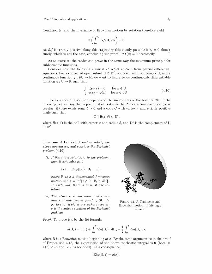
The Ito formula and applications
Condition (i) and the invariance of Brownian motion by rotation therefore yield
E(∫ τr
0
∆f(Bs)ds
)= 0.
As ∆f is strictly positive along this trajectory this is only possible if τr = 0 almostsurely, which is not the case, concluding the proof : ∆f(x) = 0 necessarily.
As an exercise, the reader can prove in the same way the maximum principle forsubharmonic functions.
Consider now the following classical Dirichlet problem from partial differentialequations. For a connected open subset U ⊂ Rd, bounded, with boundary ∂U, and acontinuous function ϕ : ∂U → R, we want to find a twice continuously differentiablefunction u : U→ R such that
∆u(x) = 0 for x ∈ Uu(x) = ϕ(x) for x ∈ ∂U
(4.10)
The existence of a solution depends on the smoothness of the boarder ∂U. In thefollowing, we will say that a point x ∈ ∂U satisfies the Poincare cone condition (or isregular) if there exists some δ > 0 and a cone C with vertex x and strictly positiveangle such that
C ∩ B(x, δ) ⊂ Uc,
where B(x, δ) is the ball with center x and radius δ, and Uc is the complement of Uin Rd.
Figure 4.1. A TridimensionalBrownian motion till hitting a
sphere.
Theorem 4.19. Let U and ϕ satisfy theabove hypotheses, and consider the Dirichletproblem (4.10).
(i) If there is a solution u to the problem,then it coincides with
v(x) := E (ϕ(Bτ ) | B0 = x) ,
where B is a d-dimensional Brownianmotion and τ = inft > 0 | Bt ∈ ∂U.In particular, there is at most one so-lution.
(ii) The above v is harmonic and conti-nuous at any regular point of ∂U. Inparticular, if ∂U is everywhere regular,v is the unique solution of the Dirichletproblem.
Proof. To prove (i), by the Ito formula
u(Bτ ) = u(x) +
∫ τ
0
∇u(Bs) · dBs +1
2
∫ τ
0
∆u(Bs)ds,
where B is a Brownian motion beginning at x. By the same argument as in the proofof Proposition 4.18, the expectation of the above stochastic integral is 0 (becauseE(τ) <∞ and |∇u| is bounded). As a consequence,
E(u(Bτ )) = u(x).
The Ito formula and applications
But the left hand side is also E (ϕ(Bτ ) | B0 = x), concluding the proof of (i).Point (ii) is more subtle. We first prove that v is harmonic. Take a ball B(x, δ) ⊂ U,
and τ = inft > 0 | Bt 6∈ B(x, δ). Then as τ 6 τ , F τ ⊂ Fτ , so using the strongMarkov property for the Brownian motion,
v(x) = Ex (ϕ(Bτ )) = Ex (Ex (ϕ(Bτ ) | F τ ))
= Ex (EBτ (ϕ(Bτ ))) = Ex(v(Bτ )) =
∫v(y)σr(dy),
where we used the invariance of B by rotation around x in the last equality, and σr isthe uniform measure, normalized to 1, on the sphere with radius r and center x. Asa consequence, using Proposition 4.18, v is harmonic in U.
We still need to prove that v is continuous at regular points. Let x ∈ ∂U be aregular point and take δ > 0, a cone C with vertex x and strictly positive angle suchthat
C ∩ B(x, δ) ⊂ Uc.
Take a given ε > 0. As ϕ is continuous on ∂U, we can chose the above δ such that
supy∈∂U∩B(x,δ)
|ϕ(y)− ϕ(x)| < ε.
For a Brownian motion B, assume that there is some 0 < θ < δ such that if |z−x| < θ,z ∈ U,
Pz(τC < τδ) > 1− ε, (4.11)
where this is the probability for a Brownian motion starting at z, τC is the hittingtime of C∩B(x, δ) and τδ is the hitting time of ∂B(x, δ). Then this would imply thatfor |z − x| < θ, z ∈ U,
|v(z)− v(x)| = |Ez(ϕ(Bτ )− ϕ(x))| 6 2‖ϕ‖∞Pz(τδ < τC) + ε 6 ε(2‖ϕ‖∞ + 1).
Hence continuity will follow if we can prove (4.11). For this, by rotation invariancewe can assume that B1 corresponds to the axis of the cone, with angle α. Note that
τC < τδ ⊂ ∪t>0
(B1(t) >
1
tanα
(B2(t)2 + · · ·+ Bd(t)
2)1/2
∩ ∩dk=1
sup[0,t]
|Bk| < c
)
for some absolute constant c > 0 depending only on δ and α. When t→ 0, these last devents have a probability converging to 1. Concerning the first event, the probabilitythat it happens for some arbitrarily small t > 0 converges to 1 as well : this is an easy
consequence of the iterated logarithm law (B1(t) gets as big as√t log(− log t) almost
surely) and the independence of B1 from the other (Bi)di=2.
Concerning links with harmonic analysis, stochastic processes yield easy proofs ofclassical statements like the following famous Liouville’s theorem.
Theorem 4.20. Let d > 1. Bounded harmonic functions on Rd are constant.
Proof. Let f : Rd → [−m,m] be an harmonic function. As a direct consequence ofthe Ito formula and harmonicity, for any t > 0
Ex (f(Bt)) = f(x) + E(∫ t
0
∇f(Bs) · dBs
)(4.12)
The Ito formula and applications
where B is a Brownian motion (beginning at x). Chose x and y distinct points in
Rd, note S (n) the sphere with center x+y2 and radius n > ‖x−y2 ‖, and H the median
hyperplane between x and y. Note
Tn = inft > 0 | Bt ∈ S (n), TH = inft > 0 | Bt ∈ H.
As |∇f | is bounded inside the sphere S (n), at time t ∧ Tn the expectation on theright hand side of (4.12) is 0, so
f(x) = Ex (f(Bt∧Tn)) = Ex (f(Bt∧Tn)1TH6t∧Tn) + Ex (f(Bt∧Tn)1TH>t∧Tn) .
The same formula holds concerning f(y), and from the reflection principle
Ex (f(Bt∧Tn)1TH6t∧Tn) = Ey (f(Bt∧Tn)1TH6t∧Tn) .
We therefore get
|f(x)− f(y)| = |Ex (f(Bt∧Tn)1TH>t∧Tn)− Ey (f(Bt∧Tn)1TH>t∧Tn)|6 2mP(TH > t ∧ Tn).
When both t and n go to ∞, this last probability converges to 0, concluding theproof.
The links between harmonic functions and the Brownian motion satisfy additionalfeatures when considering in a more specific way dimension d = 2. For example, in thefollowing discussion, it will appear that up to a time change, entire functions of the
Brownian motion are still Brownian motions. In the following, a complex process issaid to be a local martingale if both its real and imaginary parts are local martingales.
Proposition 4.21. Let Z = X + iY be a complex local martingale. Then there existsa unique complex process with finite variation beginning at 0 such that Z2 − 〈Z〉 is acomplex local martingale. Moreover, the four following statements are equivalent.
(i) The process Z2 is a local martingale.
(ii) The process 〈Z〉 is identically 0.
(iii) The brackets of the real and imaginary parts satisfy 〈X〉 = 〈Y〉 and 〈X,Y〉 = 0.
(iv) There is a Brownian motion such that Zt = B〈X〉t .
Proof. The existence of the bracket is given by
〈Z〉 = 〈X + iY,X + iY〉 = 〈X〉 − 〈Y〉+ 2i〈X,Y〉,
which satisfies all required properties. Uniqueness is a consequence of Theorem 3.26,and the equivalence between (i), (ii), (iii) is an immediate consequence of the aboveformula. Moreover, (iii) implies (iv) by the general Dubins-Schwarz Theorem 4.13,and (iv) obviously implies (iii).
A local martingale is called conformal if any of the above properties is true. Toprove that entire functions of B are conformal (this is called the conformal invarianceproperty of Brownian motion), let us first discuss the translation the Ito formula inthe complex analysis setting. We note
∂z =1
2(∂x − i∂y), ∂z =
1
2(∂x + i∂y).
. This property was used in the proof of Theorem 4.14. defined on an enlarged probability space if 〈X〉∞ <∞ with positive probability
The Ito formula and applications
A function f : C → C is called holomorphic (resp. harmonic) of ∂zf = 0 (resp.∆f = 4∂z∂zf = 0). For a general f of class C 2 and Z a conformal local martingale,the Ito formula takes the form
f(Zt) = f(Z0) +
∫ t
0
∂zf(Zs)dZs +
∫ t
0
∂zf(Zs)dZs +1
2
∫ t
0
∆f(Zs)d〈Re(Z)〉s.
As a consequence, if f is harmonic then f(Z) is a local martingale as well, and if f isholomorphic then the local martingale f(Z) has the following easy decomposition
f(Zt) = f(Z0) +
∫ t
0
f ′(Zs)dZs. (4.13)
Theorem 4.22. Let f be entire and non constant, and B a standard complex Brow-nian motion . Then f(B) is a time-changed Brownian motion :
f(Bt) = f(B0) + B〈X〉t
where B is a standard Brownian motion, and 〈X〉t :=∫ t
0|f ′(Bs)|2ds is strictly increa-
sing and converges to ∞.
Proof. As f is an entire function, so is f2, so f2(B) is a local martingale, so f(B) isa conformal local martingale. By (iv) of Proposition 4.21 there is a Brownian motion
B such thatf(Bt) = f(B0) + B〈X〉t ,
where X = Re(f(B)). From 4.13, 〈X〉t =∫ t
0|f ′(Bs)|2ds. As f ′ is entire and not
identically 0, it has a countable set of zeros so 〈X〉 is strictly increasing. It converges to∞ almost surely thanks for example to the recurrence property of the bi-dimensionalBrownian motion.
As an example the above property implies the famous d’Alembert’s theorem : anynon-constant complex polynomial has a complex zero. Let P be such a polynomial,and Z a complex Brownian motion. From the previous theorem,
P(Bt) = B〈Re(P(Bt))〉t ,
for some Brownian motion B, with the bracket going to ∞. As B is recurrent, thisimplies that for any ε > 0
z : |P(z)| 6 ε 6= ∅,
concluding the proof, the intersection of nonempty embedded closed sets being no-nempty. Another example of application for the conformal invariance property is aboutthe winding number of the bi-dimensional Brownian motion around one point. Thisis known as Spitzer’s law.
Theorem 4.23. Let B be a planar Brownian motion beginning at B0 6= 0. Define itsargument at time t, θt continuously from θ0 ∈ [0, 2π) at time 0. Then, as t→∞,
θtlog t
law−→ C
2,
where C is a standard Cauchy random variable .
. i.e. everywhere holomorphic. This means that C has density 1
π(1+x2)with respect to the Lebesgue measure.
The Ito formula and applications
Proof. By invariance by rotation and scaling, we can assume B0 = (1, 0). From Theo-
rem 4.22, if X and Y are independent standard real Brownian motions, then B definedby
B∫ t0e2Xsds = eXt+iYt
is a complex Brownian motion beginning at (1, 0). Let a > 1 and Sa = inft > 0 ||Bt| = a. We will first prove that
arg BSa
log a∼ C.
The winding number arg BSa is also the value YTlog awhere Tx = inft > 0 | Xt = x.
By scaling, proving that YT1 ∼ C is sufficient : we therefore just need to know thelaw of T1 and compose it with that of Y.
• The distribution of T1 is well-known, for example by the reflection principle2.20 :
P(T1 6 t) = P(sup[0,t]
X > 1) = P(|Xt| > 1) = P(
1
X21
6 t
),
so T1 ∼ 1/N 2 where N is a standard normal random variable.
• The density of YT1is also that of
√T1Y1, by conditioning on T1. Hence it has
the same law as N ′/N , both random variables being independent and standardGaussian. This is known to be a Cauchy distribution (for example by calculatingthe characteristic function).
From the previous discussion,arg BS√t
log t∼ C
2,
hence the proof will be complete if we can show that
arg Bt − arg BS√t
log t
converges to 0 in probability. For this, consider τ the inverse of the clock, defined by∫ τt
0
e2Xsds = t.
For some parameters δ ∈ (0, 1) (it will go to 0) such that δ√t > 1 and λ > 0 (it will
go to ∞), consider the events
A =
Sδ√t 6 t 6 Sδ−1
√t
,
B =
sup[τS
δ√t,τS
δ−1√t]
|Ys −YτSδ√t| 6 λ
2
.
Then A∩B ⊂| arg Bt − arg BS√t
| 6 λ
, so we just need to prove that the probability
of A goes to 1 as δ → 0, and that of B goes to 1 as λ→∞, for any given δ.
• Concerning A things are easy because
|Bt| > δ√t ∩ sup
[0,t]
|Bs| < δ−1√t ⊂ A,
and both events have a probability going to 1 a δ → 0, independently of t byscaling.
The Ito formula and applications
• Concerning B, note that
τSa = infu > 0 | Xu = log a,
so from the strong Markov property
τSδ−1√t− τSδ√t ∼ T−2 log δ,
where as previously Tx = inft > 0 | Xt = x. As Y is independent from X, thismeans that
sup[τS(δ
√t),τS(δ−1
√t)]
|Ys −YτS(δ√t)| ∼ sup
[0,∆]
|Ys|,
where ∆ is an almost surely finite random variable independent of Y, and withlaw depending on δ but not on t. As a consequence, P(B) is independent of tand goes to 1 as λ→∞.
This concludes the proof.
4. The Girsanov theorem
In this section, the influence of the probability measure P on the semimartingalenotion is discussed. As an example a probability space (Ω,F , (F t)06t61,P), and aBrownian motion B on this space, one can define a new probability measure by
dQdP
=sup[0,1] B
E(
sup[0,1] B) .
The process B is certainly not a Q-Brownian motion, as the symmetry propertydoes not hold anymore, but is-it a Q-semimartingale ? The main motivations for suchquestions are the following :
• practicing importance sampling on trajectories spaces ;
• deriving properties of the Wiener measure itself by looking at its behavior undersome transformations ;
• just like changing variables allows to solve equations, changing the measure onthe path space is the main tool to perform some expectations.
Before stating the general result, we need the following two propositions.
Proposition 4.24. Assume Q P on F(= F∞). For t ∈ [0,∞], note
Dt =dQdP
∣∣∣∣Ft.
(i) The process D is a uniformly integrable martingale.
(ii) If D is assumed right-continuous , then for any stopping time T
DT =dQdP
∣∣∣∣FT
.
(iii) If D is assumed right-continuous, and Q ∼ P on F then, for any t > 0, Dt > 0.
. This is not a very restrictive hypothesis, one can show that there is always a right-continuousversion of the process D, see [12].
The Ito formula and applications
Proof. For (i), note that for any t > 0 and A ∈ F t
EP(1ADt) = EQ(1A) = EP(1AD) = EP(1A E(D | F t)).
where D = dQdP∣∣F . By uniqueness of the Radon-Nikodym derivative, this implies Dt =
E(D | F t) almost surely, concluding the proof as D ∈ L1.Point (ii) relies on the stopping time Theorem 3.13, which implies that DT =
E(D | FT). As a consequence, for any A ∈ FT,
EP
(1A
dQdP
∣∣∣∣FT
)= EQ(1A) = EP(1AD) = EP(1ADT),
so DT = dQdP∣∣FT
.
Finally, (iii) follows from (ii) : for T = inft > 0 | Dt = 0, by right-continuityDT = 0 on T <∞, so
Q(T <∞) = EP(1T<∞DT) = 0.
As Q P, this implies P(T <∞) = 0, as expected.
Proposition 4.25. Let D be a strictly positive continuous local martingale. Thenthere exists a unique continuous local martingale L such that
Dt = E(L)t := eLt− 12 〈L〉t .
Proof. For uniqueness, note that if L and L are solutions, then
L− L =1
2
(〈L〉 − 〈L〉
)is a finite variation process and also a local martingale, so it is indistinguishable from0. For the existence, the choice
Lt = log D0 +
∫ t
0
dDs
Ds
makes sense as D is strictly positive and, by the Ito formula,
log Dt = log D0 +
∫ t
0
dDs
Ds− 1
2
∫ t
0
d〈D〉sD2s
= Lt −1
2〈L〉t,
concluding the proof.
Both results imply the following, known as Girsanov’s theorem, or Cameron-Martin’s theorem in the special case of deterministic shifts.
Theorem 4.26. Let Q ∼ P on F . Assume that the process defined by
Dt =dQdP
∣∣∣∣Ft
is continuous, and write it as D = E(L), with L a local martingale. Then if M is aP-local martingale the process
M := M− 〈M,L〉
is a Q-local martingale.
. This is possible by Proposition 4.24 (iii) and Proposition 4.25
The Ito formula and applications
Proof. We first prove that if a process XD is a P-local martingale, then X is a Q-local martingale. For this, we show that for T any stopping time and X a continuousadapted process such that (XD)T is a P-martingale, then XT is a Q-martingale :
• First the integrability condition is satisfied : from Proposition 4.24 (ii),
EQ(|XTt |) = EP(|XT
t ||DTt |) <∞
because (XD)T is a P-martingale.
• Moreover, for s < t and A ∈ Fs, still using Proposition 4.24 (ii) for the secondand fourth equalities, and the martingale property for (XD)T in the third one,
EQ(1AXTt ) = EQ(1A∩T6sX
Tt ) + EQ(1A∩T>sX
Tt )
= EP(1A∩T6sXTt Dt∧T) + EP(1A∩T>sX
Tt Dt∧T)
= EP(1A∩T6sXTs Dt∧T) + EP(1A∩T>sX
Ts Ds∧T)
= EQ(1A∩T6sXTs ) + EQ(1A∩T>sX
Ts )
= EQ(1AXTs ).
Hence XTs = EQ(XT
t | Fs).
Thanks to the previous discussion, MD being a P-local martingale is enough to
prove that M is a Q-local martingale. The Ito formula yields
d ((M− 〈M,L〉)D)t = (M− 〈M,L〉)tdDt + (dMt − d〈M,L〉t)Dt + d〈M,D〉t= (M− 〈M,L〉)tdDt + (dMt − d〈M,L〉t)Dt + Dtd〈M,L〉t= (M− 〈M,L〉)tdDt + DtdMt,
where in the second equality we used the fact that dDt = DtdLt. So MD is a stochasticintegral with respect to the P-local martingales D and M, so it is a P-local martingale,concluding the proof.
One particularly interesting case of the above result is the case when M is a P-Brownian motion.
Corollary 4.27. One can replace local martingale by Brownian motion in the hypo-thesis and conclusion of Theorem 4.26.
Proof. If M is a P-Brownian motion, then M is a Q-local martingale (by Girsanov’stheorem) and its bracket is t (by the sum of quadratic increments formula in Theorem3.26, the bracket does not depend on the underlying probability measure), so Levy’scriterion Theorem 4.11 applies.
The condition Q ∼ P on F in the hypothesis of the Girsanov theorem is quite res-trictive. The following lines explain why, and a way to overcome this. As an example,if M = B is a Brownian motion, one could try to use Girsanov’s theorem till infinite
time to study the properties of the Brownian motion with drift M = (Bt − νt, t > 0).For this, we want a measure Q on F such that for any t > 0
dQdP
∣∣∣∣Ft
= eνBt− ν2
2 t. (4.14)
By Theorem 1.3.5 in [18], such a measure Q exists. But it is not absolutely continuouswith respect to the Wiener measure P : the reader could prove that if ν > 0 the eventlim inf Bt/t > 0 is almost sure for Q and its complement is almost sure for P. Toavoid this problem, the applications of the Girsanov theorem can be performed up
The Ito formula and applications
to a finite horizon : if Q ∼ P on F t, then M is a Q-local martingale when one onlyconsiders its restriction to [0, t] : this is true by applying the general statement witha modified filtration such that Fu = F t when u > t.
Coming back to (4.14), we get that (Bs − νs, 0 6 s 6 t) is a Q-Brownian motion,hence for any bounded continuous functional F,
EQ (F(Bs − νs, 0 6 s 6 t)) = EP (F(Bs, 0 6 s 6 t)) .
When F is a cylindric function, this is just a change of variables formula for finite-dimensional Gaussian measures. If F depends only on the trajectory up to a stoppingtime T 6 t a.s. the above equation together with Proposition 4.24 (ii) yield
EP
(F(Bs − νs, 0 6 s 6 T)eνBT− ν
2
2 T)
= EP (F(Bs, 0 6 s 6 T)) . (4.15)
As an example of application, the above equation allows to prove the following law ofhitting time of a Brownian motion with drift.
Corollary 4.28. Let T(ν)a = infs > 0 | Bs + νs = a. Then for any λ > 0
EP
(1
T(ν)a <∞e
−λT(ν)a
)= eνa−|a|
√2λ+ν2
.
Proof. Consider the random variable F = 1T
(ν)a 6t
e−λT(ν)a (which is F t∧Ta -measurable)
in (4.15). Then
EP
(1
T(0)a 6t
e−λT(0)a e
νBt∧T(0)
a − ν22
T(0)a
)= EP
(1
T(ν)a 6t
e−λT(ν)a
).
Dominated convergence as t→∞ yields
EP
(1
T(0)a <∞e
−(λ+ ν2
2
)T(0)a eνa
)= EP
(1
T(ν)a <∞e
−λT(ν)a
).
The left hand side is known thanks to Corollary 3.17, so
EP
(1
T(ν)a <∞e
−λT(ν)a
)= eνa−|a|
√2λ+ν2
,
the expected result.
A simple yet sometimes useful consequence of Girsanov’s theorem is that theWiener measure gives positive mass to any open subset of continuous functions on[0, 1].
Corollary 4.29. Let f be continuous on (0, 1), f(0) = 0, and note Vε(f) the set ofcontinuous functions g on (0, 1), beginning at 0, such that sup(0,1) |f(x) − g(x)| < ε.
Then P(Vε) > 0.
Proof. First, for a given ε > 0, there exists a continuous f0, beginning at 0, such thatits ε-neighborhood has a strictly positive probability (otherwise the measure would benull). We want to prove it for general f By interpolation and up to choosing a smallerε, we can suppose that h := f − f0 is C 1. In the Girsanov theorem take M = B, a
Brownian motion, and Lt =∫ t
0hsdBs. Then M− 〈M,L〉 is B− h, and
P(|B− f |L∞(0,1) < ε
)= EP
(1|B−f0|L∞(0,1)<εe
∫ 10hsdBs− 1
2
∫ 10h2sds).
This right hand side is strictly positive because P(|B− f0|L∞(0,1) < ε
)> 0 and∫ 1
0hsdBs > −∞ almost surely.
The Ito formula and applications
We finally consider the question of checking the hypotheses to apply Girsanov’stheorem. In most applications, a P-local martingale L is given, and one makes thechoice
dQdP
∣∣∣∣Ft
= eLt− 12 〈L〉t ,
hoping that the expectation of the right hand side is 1. Note that E(L) is a positivelocal martingale, hence a supermartingale, hence it converges almost surely and
E (E(L)∞) 6 1. (4.16)
There is equality if and only if E(L) is a uniformly integrable martingale. Moreover,if E(L) is uniformly integrable, then when defining
dQdP
∣∣∣∣F
= E(L)∞,
we obviously have Q ∼ P. Hence, checking the uniform integrability of an exponentiallocal martingale is important to apply Girsanov’s theorem, and a famous criteriumby Novikov is given hereafter.
Theorem 4.30. Let L be a local martingale beginning at 0. If
E(e
12 〈L〉∞
)<∞, (4.17)
then E(L) is a uniformly integrable martingale.
Proof. We first prove that (4.17) implies that L is uniformly integrable and that
E(e
12 L∞
)<∞, which in turn implies the result, as we will see after.
Obviously, by (4.17) E(〈L〉∞) < ∞, so L is bounded in L2 by Theorem 3.29.Hence L is a uniformly integrable martingale. Moreover, by a simple application ofthe Cauchy-Schwarz inequality and using (4.16),
E(e
12 L∞
)= E
(E(L)
12∞
(e
12 〈L〉∞
) 12
)6 E (E(L)∞)
12 E(e
12 〈L〉∞
) 12
6 E(e
12 〈L〉∞
) 12
,
so E(e
12 L∞
)< ∞. Now, we want to prove the uniform integrability of E(L). From
the discussion before Theorem 4.30, a sufficient condition is E(E(L)∞) = 1.
• First, as L is uniformly integrable, Lt = E(L∞ | F t), so by convexity e12 Lt <
E(e
12 L∞ | F t
). This proves that (e
12 Lt , t > 0) is uniformly integrable.
• Moreover, as the exponential is convex and increasing, (e12 Lt , t > 0) is a submar-
tingale, uniformly integrable from the previous point. Hence, for any stopping
time T, e12 LT < E
(e
12 L∞ | FT
): the family
e 12 LT | T stopping time
. If this is a uniformly integrable martingale, obviously we need to have E (E(L)∞) = 1 by thestopping time theorem. Reciprocally, if we have equality, as the function t 7→ E (E(L)t) decreases, itneeds to be constant. Hence, for t > s, E(E(E(L)t | Fs)− E(L)s) = 0, and as the integrated term isnon-positive, we have E(E(L)t | Fs) = E(L)s almost surely : E(L) is a martingale. Moreover, as aneasy consequence of Fatou’s lemma
E(L)t > E(E(L)∞ | Ft),and as both random variables above have the same expectation they are equal : E(L)t > E(E(L)∞ |Ft), so E(L) is uniformly integrable.
The Ito formula and applications
is uniformly integrable.
• We would like to prove that E(L)T | T stopping time is uniformly inte-grable. This is slightly too much required. We can show that E(λL)T |T stopping time is uniformly integrable for any 0 < λ < 1. Take any A ∈ F(typically, A = E(λL)T > x). Then
E (1AE(λL)T) = E(1A(E(L)T)λ
2
eλ(1−λ)LT
)6 E (E(L)T)
λ2
E(1Ae
λ1+λLT
)1−λ2
6 E(1Ae
λ1+λLT
)1−λ2
= E((
1Ae12 LT
) 2λ1+λ
)1−λ2
6 E(1Ae
12 LT
)2λ(1−λ)
where we used in the second inequality that for a positive supermartingale Mand any stopping time T, E(MT) 6 M0 (this is true for bounded stopping times,and then for any of them by Fatou). The last inequality relies on the concavityof x 7→ xa when a < 1. The last term above being uniformly integrable (fromour second point), the set E(λL)T | T stopping time is uniformly integrablefor any 0 < λ < 1.
• This implies that E(λL) is a uniformly integrable martingale.As a consequence,
1 = E (E(λL)∞) 6 E (E(L)∞)λ2
E(e
12 L∞
)2λ(1−λ)
.
Taking λ→ 1− yields E(E(L)∞) > 1.
This achieves the proof.

Chapter 5
Stochastic differential equations
Ordinary differential equations aim to find, from local data
dXt
dt= b(Xt),
a global solution X. Some criteria on b (e.g. the Cauchy-Lipschitz theorem) yield toexistence and uniqueness of solutions to such equations. They describe the evolutionof a deterministic physical system. A random perturbation of such a system is per-tinent in many contexts : to study stability of such trajectories (e.g. bifurcations indynamical systems), or directly because the physics of the deterministic problem aretoo intricate, hence this mixing property is simplified as an independence hypothesis(e.g. pollen particles floating in water) or directly because the physical assumption in-cludes randomness (e.g. quantum mechanics). Such a random equation can be writtenas
dXt = σ(Xt)dBt + b(Xt)dt.
The meaning to give to this local evolution is that X is a semimartingale such that,almost surely, for any t > 0,
Xt = X0 +
∫ t
0
(σ(Xs)dBs + b(Xs)ds).
Note first that these random perturbations of ordinary differential equations are per-formed through a Gaussian noise. This is not very restrictive : by the Donsker Theorem2.26, any independent increments in L2 lead to a Brownian motion. A more subtlediscussion is required concerning whether the solution of the stochastic differentialequation is a deterministic function of the random trajectory B (strong existence anduniqueness of the solution) or if it given by a law of the trajectory (weak uniqueness ofthe solution). This point is the purpose of the next section. In Section 2, an analogueof the Cauchy-Lipschitz theorem for the existence of strong solutions is given, basedof Picard’s iteration as well. The strong Markov property associated to these solutionswill allow us to discuss generalizations of the Dirichlet problem, already considered inChapter 4, when the second order differential operator is not necessarily the EuclideanLaplacian anymore (Section 3). After that, a practical way to perform simulations ofstochastic differential equations (e.g. for Monte Carlo purpose) is given, as one (of themany) application(s) of the Stroock-Varadhan martingale problems theory (Section4). Finally, we will study in details the case σ ≡ 1, pertinent in filtering theory andrevealing a wide variety of existence/uniqueness cases, in Section 5.
1. Weak and strong solutions
In the following definition, σ and b depend not only on the current point Xt butalso on t and the entire trajectory till time t. Moreover, they are assumed to bemultidimensional :
σ = (σij)16i6d,16j6m, b = (bi)16i6d,
each σij , bi, being a function from R+ × C to R, σ(t, ω), b(t, ω) ∈ Xt where Xt =σ(ωs, s 6 t).
Stochastic differential equations
Definition 5.1. A solution to the equation
dXt = σ(t,X)dBt + b(t,X)dt
on R+ is the collection of :
• a filtered probability space (Ω,F , (Ft)t>0,P) ;
• a (Ft)-Brownian motion B = (B(1), . . . ,B(m)) with B(i) a (Ft)-martingale and
〈B(i),B(j)〉t = 1i=jt ;
• a (Ft)-adapted process X = (X(1), . . . ,X(d)) such that
Xt = X0 +
∫ t
0
σ(s,X)dBs +
∫ t
0
b(s,X)ds.
This is abbreviated by saying that the process X is a solution of E(σ, b). When imposedto X0 = x, X is said to be a solution of Ex(σ, b).
This definition has an obvious extension to the solution of the stochastic differentialequation with a finite time horizon T. The main notions of uniqueness and existenceare the following.
Definition 5.2. For the equation E(σ, b), we say that there is
• weak existence if for any x ∈ Rd there is a solution to Ex(σ, b) ;
• weak existence and uniqueness is for any x ∈ Rd there is a solution to Ex(σ, b)and all solutions to Ex(σ, b) have the same law ;
• pathwise uniqueness if, given (Ω,F , (Ft)t>0,P) and B, two solutions X and X′
such that X0 = X′0 P-almost surely cannot be distinguished.
Moreover, a solution X of Ex(σ, b) is said to be strong if X is (Bt)-adapted, whereBt = σ(Bs, s 6 t).
We now want to illustrate the above definitions by some examples. Suppose givena Brownian motion (βt)t>0 on a probability space (Ω,F , (Ft)t>0,P), for exampleFt = σ(βs, s 6 t) and P is the Wiener measure.
• Weak existence. Consider the stochastic differential equation
dXt = 3 sgn(Xt)|Xt|2/3dBt + 3 sgn(Xt)|Xt|1/3dt, X0 = 0.
From Ito’s formula, Xt = B3t is a solution.
• Weak uniqueness. Consider the equation
dXt = f(Xt)dBt
where f : R → R is any measurable function with |f(x)| = 1 for any x ∈ R.Then any solution X of the equation is a F-martingale with bracket 〈X〉t = t,hence it is a Brownian motion. This proves uniqueness in law.
• Pathwise uniqueness. The following equation is the one describing the so-calledgeometric Brownian motion :
dXt = XtdBt, X0 = 1.
Then B = β, Xt = eBt− t2 is a solution. Given (Ω,F , (Ft)t>0,P) and B, if Yt isanother solution, from the Ito formula
d
(Yt
Xt
)=
dYt
Xt− YtdXt
X2t
+Yt
X3t
d〈X〉t −1
X2t
d〈X,Y〉t = 0.
Consequently X and Y cannot be distinguished.
Stochastic differential equations
• Weak existence with no weak uniqueness. Consider the same equation as pre-viously,
dXt = 3 sgn(Xt)|Xt|2/3dBt + 3 sgn(Xt)|Xt|1/3dt, X0 = 0.
From Ito’s formula, B = β and Xt = B3t are solutions, as well as X = 0. This
example shows as well that there can be various strong solutions.
• Weak existence and weak uniqueness with no pathwise uniqueness. From theoriginal Brownian motion β, define another Brownian motion (Levy’s criterion)by
Bt =
∫ t
0
sgn(βs)dβs,
where sgn(x) = 1 if x > 0, -1 otherwise. Then β and −β are solutions of
dXs = sgn(Xs)dBs, X0 = 0,
because∫ t
01βs=0ds = 0, hence
∫ t01βs=0dBs = 0. Moreover, any solution is a
Brownian motion, once again by Levy’s criterion.
Section 5 will in particular give an example of weak existence, weak uniqueness,and non existence of a strong solution. Note that one cannot have pathwise uniquenessand no weak uniqueness, or pathwise uniqueness and solutions not measurable in B’scanonical filtration, this is a famous result of Yamada and Watanabe.
Theorem 5.3. If for the equation E(σ, b) pathwise uniqueness holds, then there isalso weak uniqueness, and any solution is strong.
Proof. For notational convenience, we consider the case d = m = 1. Proving thetheorem for Ex(σ, b) is sufficient, by conditioning on the initial value. Note that somecare is needed for this conditioning , as the event has no positive measure. However,as C (R+,R2) is a Polish space, there is a regular conditional distribution P(ω, ·) of P,the law of (X,B), with respect to B0. See [16] for more details about this conditioning.
Let (B,X) and (B′,X′) be two solutions to Ex(σ, b), eventually defined on distinctprobability spaces. We note W = C (R+,R), with the compact uniform topology,B(W) the topological Borel field on W, Bt(W) = σ(ωs, s 6 t). The same objects areeasily defined on W×W,W×W×W. Let P(dω,dω′) (resp. P′) be the law of (B,X)(resp. (B′,X′)) on (W ×W,B(W ×W)). Finally, we introduce Pω(dω′) the regularconditional distribution of P(dωdω′) given ω, i.e.
(i) for any ω ∈W, this is a probability measure on (W,B(W)),
(ii) for any A ∈ B(W), Pω(A) is B(W)-measurable as a function of ω,
(iii) for any (A,A′) ∈ B(W ×W),
P(A×A′) =
∫A′
Pω(A)R(dω)
where R is the law of B on (W,B(W)), i.e. the Wiener measure.
For the existence of this regular conditional distribution, we refer to [9]. In the sameway we define P′ω(dω).
To make use of pathwise uniqueness in the proof, we need to consider both solu-tions (B,X) and (B′,X′) in the same probability space. For this purpose, let Q be theprobability distribution defined on (W ×W ×W,B(W ×W ×W)) by
Q(dω1dω2dω) = Pω(dω1)P′ω(dω2)R(dω). (5.1)
Stochastic differential equations
Note that the projection of Q on along the second coordinate is P, and P′ along thefirst coordinate. We want to prove that ω is a (Q,B(W×W×W)t) Brownian motion.Let F1,F2,F be three Bt(W)-measurable functions, and u > t. Then
EQ ((ω(u)− ω(t))F1(ω1)F2(ω2)F(ω))
=
∫W
(ω(u)− ω(t))
(∫W
Pω(dω1)F1(ω1)
)(∫W
Pω(dω2)F2(ω2)
)F(ω)R(dω).
By the following important Lemma 5.4,∫
WPω(dω1)F1(ω1) and
∫W
Pω(dω2)F2(ω2)
are Bt(W)-measurable in ω, so by conditioning on Bt(W) and using that ω is a(R, (Bt))-martingale (a Brownian motion actually), the above term vanishes. In thesame way,
EQ
(((ω(u)− ω(t))2 − (u− t)2
)F1(ω1)F2(ω2)F(ω)
)= 0,
so ω is a (Q, (Bt(W×W×W)))-martingale with bracket 〈ω〉s = s : it is a (Q, (Bt(W×W×W)))-Brownian motion. To sum up, we have proven that on the probability space
(W ×W ×W,B(W ×W ×W), (Bt(W ×W ×W)),Q)
the processes (B,X) := (ω, ω1) and (B′,X) := (ω, ω2) are solutions to Ex(σ, b). Bypathwise uniqueness, ω1 = ω2 Q-almost surely. Looking back at (5.1), this implies thatP = P′ and there is a B(W)-measurable function F such that ω1 = F(ω), ω2 = F(ω).By Lemma 5.4, F is adapted, hence any solution is strong.
Lemma 5.4. Let P(dωdω1) be the law of (B,X), a solution of Ex(σ, b).For A ∈ Bt(W), the applications ω → Pω(A) and ω → P′ω(A) are Bt(W)-
measurable.
Proof. If σ1, σ2, σ are three σ-algebras such that σ1 ∨ σ2 is independent of σ under aprobability measure µ, it is a general fact that for A ∈ σ1, µ-almost surely
µ(A | σ2) = µ(A | σ2 ∨ σ).
We apply this to σ1(t) = σ(ω1(s), s 6 t), σ2(t) = σ(ω(s), s 6 t), σ(t) = σ(ω(u) −ω(t), u > t) and the measure P(dωdω1). As, for some filtration (Ft), ω is a (Ft)-Brownian motion, and X is (Ft)-adapted, we have σ1(t) ∨ σ2(t) independent of σ(t).Hence the above result reads, P-almost surely
P(·,A) = EP(1A | σ2(∞)) = P(·,A) = EP(1A | σ2(t) ∨ σ(t)) = EP(1A | σ2(t)),
which is obviously Bt(W)-measurable.
2. The Lipschitz case
Like for ordinary differential equations, we will show existence and strong unique-ness for E(σ, b) under the Lipschitz hypothesis
|σ(t, ω)− σ(t, ω′)|+ |b(t, ω)− b(t, ω′)| 6 c sups6t|ω(s)− ω′(s)|.
Theorem 5.5. Under the above hypothesis, there is pathwise uniqueness for E(σ, b).Moreover, for any filtered probability space (Ω,F , (Ft)t>0,P), any F-Brownian motion
B, and any x ∈ Rd there is a strong solution to Ex(σ, b).
Remark. There is only one strong solution in the above theorem, by pathwise uni-queness. Moreover, the above result also proves weak existence, and by the Yamada-Watanabe theorem weak uniqueness.
Stochastic differential equations
Proof. We assume m = d = 1 to simplify notations, the general case being absolutelysimilar. We first prove pathwise uniqueness : given (Ω,F , (Ft)t>0,P), a F-Brownianmotion B, let X and X′ be two solutions of the related stochastic differential equationsuch that X0 = X′0 almost surely. To avoid integrability problems, consider L > 0 andthe stopping time
τ = inft > 0 | |Xt| > L or |X′t| > M.Then, for any t > 0,
Xt∧τ = X0 +
∫ t∧τ
0
σ(s,X)dBs +
∫ t∧τ
0
b(s,X)ds,
and a similar equation holds for X′. Consequently, assuming that t lies in a boun-ded set [0,T] and using the elementary identity (a + b)2 6 2(a2 + b2), f(t) =
E(sups6t(Xs∧τ −X′s∧τ )2
)is bounded by
2E
(sups6t
(∫ s∧τ
0
(σ(u,X)− σ(u,X′))dBu
)2)
+ 2E
(sups6t
(∫ s∧τ
0
(b(u,X)− b(u,X′))du)2).
By the Doob (resp. Cauchy-Schwarz) inequality for the σ (resp. b) term, this is lowerthan
8E
((∫ t∧τ
0
(σ(s,X)− σ(s,X′))dBs
)2)
+ 2TE(∫ t∧τ
0
(b(s,X)− b(s,X′))2ds
)= 8E
(∫ t∧τ
0
(σ(s,X)− σ(s,X′))2ds
)+ 2TE
(∫ t∧τ
0
(b(s,X)− b(s,X′))2ds
).
We used that the expectation of the square of a martingale is also the expectation ofits bracket (the stochastic integral is L2-bounded thanks to the stopping time τ andthe boundedness of σ by the Lispschitz hypothesis). Now, we can use the Lipschitzhypothesis on σ and b to obtain finally
f(t) 6 2c2(4 + T)
∫ t
0
f(s)ds.
As X0 = X′0 almost surely, f(0) = 0 a.s. and Gronwall’s lemma applied to the aboveinequality yields f(t) = 0 a.s. for any t ∈ [0,T], hence for any t > 0. This means thatalmost surely, for any t ∈ [0,T], Xt∧τ = X′t∧τ . By making L → ∞, the processes Xand X′ cannot be distinguished.
Now, given a probability space (Ω,F , (Ft)t>0,P), a F-Brownian motion B, andany initial value x, one can construct a solution to Ex(σ, b) which is adapted to thecanonical filtration (Bt)t>0 of B using Picard’s approximation scheme :
X(0)t = x,
X(n)t =
∫ t0σ(s,X(n−1))dBs +
∫ t0b(s,X(n−1))ds.
These processes are properly defined as an immediate induction shows that for anyn > 0, X(n) is B-adapted, and still by induction for any T > 0 and any n > 0 there isa constant c(n) such that
E(
supt6T
(X
(n)t
)2)
6 c(n). (5.2)
. This lemma states in particular that if, on R+, f ′(t) 6 af(t), then f(t) 6 f(0)eat. Proof :
f(t)e−at decreases, by differentiation and application of the hypothesis.
Stochastic differential equations
This is obvious at rank n = 0. Assuming the property at rank n − 1, the rankn case follows by using the Lipschitz conditions (in particular |σ(t, ω)| 6 c′ +c sup[0,T] ω, |b(t, ω)| 6 c′+c sup[0,T] ω for any t ∈ [0,T]) and the identity (a+b+c)2 6
3(a2 + b2 + c2), by convexity of x→ x2 :
E(
supt6T
(X
(n)t
)2)
63|x|2 + 3E
(supt6T
(∫ t
0
σ(s,X(n−1))dBs
)2)
+ 3E
(supt6T
(∫ t
0
b(s,X(n−1))ds
)2)
63|x|2 + 12E
(∫ T
0
σ(s,X(n−1))dBs
)2+ 3TE
(∫ t
0
b(s,X(n−1))2ds
)
=3|x|2 + 12E
(∫ T
0
σ(s,X(n−1))2ds
)+ 3TE
(∫ t
0
b(s,X(n−1))2ds
)
63|x|2 + 12
∫ T
0
(c′ + cE(sup
u6sX(n−1))
)2
ds+ 3T
∫ T
0
(c′ + cE(sup
u6sX(n−1))
)2
ds
63(|x|2 + 2T(4 + T)(c′2 + c2c(n−1)))
where we used in the first inequality the Doob and the Cauchy Schwarz inequality aspreviously in the proof. This achieves the inductive proof of (5.2) by taking the above
constant for c(n).The a-priori local martingale
∫ t0σ(s,X(n))dBs is actually a L2-bounded martingale
from the above estimate (5.2). This allows the following upper bound for the infinite
norm between X(n+1) and X(n) on [0,T], along the same steps as previously :
E
(sup[0,t]
(X(n+1) −X(n))2
)62E
(sups6t
(∫ s
0
(σ(u,X(n+1))− σ(u,X(n))
)dBu
)2)
+ 2E
(sups6t
(∫ s
0
(b(u,X(n+1))− b(u,X(n))
)du
)2)
68E((∫ t
0
(σ(s,X(n+1) − σ(s,X(n)))dBu
)2))
+ 2TE(∫ t
0
(b(s,X(n+1))− b(s,X(n))
)2
du
)E
(sup[0,t]
(X(n+1) −X(n))2
)62(4 + T)c2 E
(∫ t
0
sup06v6u
(X(n+1)u −X(n)
u )2du
).
This can be written, for t ∈ [0,T], f (n+1)(t) 6 cT∫ t
0f (n)(u)du, with f (n+1)(t) =
E(
sup[0,t](X(n+1) −X(n))2
), cT = 2(4 + T)c2. An immediate induction therefore
yields
f (n)(t) 6
(sup[0,T]
f (0)(s)
)(cT)n
tn
n!.
In particular,∑∞n=0
√f (n)(T) <∞, i.e.∑
n
‖sup[0,T]
(X(n+1) −X(n))‖L2 <∞,
so∑n sup[0,T](X
(n+1) −X(n)) is bounded in L2, hence a.s. finite : almost surely X(n)
converges uniformly on [0,T] to a continuous process X. As X(n) is adapted to thecanonical filtration of B, X is adapted as well.
Stochastic differential equations
We now need to check that X is a solution of Ex(σ, b) : as ‖sup[0,T](X(n)−X)‖L2 6∑∞
m>n
√f (m)(T)→ 0, the similar inequalities as previously imply that, in L2
∫ t
0
σ(s,X(n))dBs →∫ t
0
σ(s,X)dBs,∫ t
0
b(s,X(n))dBs →∫ t
0
b(s,X)ds.
Injecting this in the induction relation between X(n) and X(n−1), we get that
Xt =
∫ t
0
σ(s,X)dBs +
∫ t
0
b(s,X)ds,
first in L2 but almost surelyas well.
3. The Strong Markov property and more on the Dirichlet problem
4. The Stroock-Varadhan piecewise approximation
This section is devoted to approximations of the law of stochastic processes. Howcan one make a reasonable simulation of the trajectory of the strong solution ofa stochastic differential equation ? More generally, the Stroock-Varadhan piecewiseapproximation [18] provides the convergence in law of a discrete Markov chain to thesolution of a martingale problem.
The reason why we consider their approach is that it ensures convergence in lawof processes under very weak conditions, provided that the associated martingaleproblem admits a unique solution.
4.1. Martingale problems
The Stroock-Varadhan approach allows to define Markov processes through theirgenerator with no explicit construction of the semigroup. In the case of diffusions,two other classical representations of diffusions are the following.
• Kolmogorov and Feller expressed the transition probabilities as the solution ofa forward partial differential equation.
• Ito introduced its stochastic calculus and therefore represents the diffusions assolutions of stochastic differential equations.
Consider σ a d× d matrix function, a = σ tσ and b : Rd → Rd, all of them beingmeasurable.
Definition 5.6. A process (Xt, t > 0) with values in Rd, together with a filteredprobability space (Ω,F , (F)t,P), is said to solve the martingale problem M(a, b) if forany 1 6 i, j 6 d
Yi := (Xit −∫ t
0bi(Xs)ds, t > 0),
(YitY
jt −
∫ t0aij(Xs)ds, t > 0),
are local martingales. If a solution to M(a, b) has a unique possible law, the problemis said to be well posed.
. If Yn converges to Y1 in L2 and Y2 a.s., then Y1 = Y2 almost surely : Yn converges to Y2 inprobability, hence almost surely along a subsequence ; by uniqueness o the limit, Y1 = Y2.
Stochastic differential equations
We will study the martingale approach for the following reason : Theorem 5.9hereafter states the weak convergence of discrete time Markov processes towards so-lutions of sde under the uniqueness condition of the the solution of the limiting martin-gale problem. This is a more general condition than pathwise uniqueness for example.Very general conditions for well-posedness of M(a, b) are given in [18]. For example,in dimension 1, measurability, boundedness for a and b and uniform positivity for aare sufficient.
Moreover, a martingale problem is well-posed if and only if there is uniquenessin law for an associated stochastic differential equation. More precisely, if σ and bare Lipschitz, there exists a unique strong solution (i.e. a filtered probability space(Ω,F , (F)t,P), Ft = σ(Bs, s 6 t) where B = (B1, . . . ,Bd) is a Brownian motion andan F-adapted X) to the stochastic differential equation E(a, b) :
dXt = σ(Xt)dBt + b(Xt)dt.
Then X together with (Ω,F , (F)t,P) solves the martingale problem M(a, b), a = σ tσ.An interesting point is that a reciprocal is true, with weaker assumptions on σ, b. Fortechnical reasons, we assume that b is continuous and a = σ tσ is elliptic, but thesehypotheses can be seriously weakened, as remarked later.
Theorem 5.7. Assume the above hypotheses and that X, (Ω,F , (F)t,P) is a solutionto M(a, b). Then there exists a F-Brownian motion B in Rdsuch that X,B solvesE(σ, b).
Proof. In the following, all (stochastic) integrals make sense thanks to our (strong)assumptions on a and b. As X is a solution of M(a, b),
Yi := (Xit −∫ t
0
bi(Xs)ds, t > 0)
is a local martingale, and d〈Yi,Yj〉t = aij(t)dt. Let
Bi :=
(∫ t
0
d∑k=1
(σ−1)ik(Xs)dYks , t > 0
). (5.3)
This is a local martingale and the joint brackets are
〈Bi,Bj〉t =
d∑k,l=1
∫ t
0
(σ−1)ik(Xs)(σ−1)jl(Xs)(σ
tσ)kl(Xs)ds.
But the definition of the inverse yields
d∑k,l=1
(σ−1)ik(σ−1)jl(σtσ)kl =
d∑k,l,m=1
(σ−1)ik(σ−1)jl(σ)k,mtσml = 1i=j .
By Levy’s criterion, the Bi’s are Brownian motions, and from (5.3)
dXt = σ(Xt)dBt + b(Xt)dt,
which concludes the proof.
Remark. This result of the theorem actually holds under weaker hypotheses, in par-ticular without the invertibility/ellipticity condition, by letting B go independentlyfor any time s such that σ(Xs) is not invertible.
Stochastic differential equations
4.2. Convergence of Markov chains
Consider a Markov chain (U(ε)n )n>0, depending on a parameter ε > 0, with a
transition kernel P(ε) :
P(U(ε)n+1 ∈ B | U(ε)
n = x) = P(ε)(x,B).
In the context of the strong solution a stochastic differential equation in Rd (e.g. withLipschitz coefficients),
dXt = σ(Xt)dBt + b(Xt)dt,
one can think about U(ε)n+1 as
U(ε)0 = U0,
U(ε)n+1 = U
(ε)n + σ(U
(ε)n )√εNn + b(U
(ε)n )ε,
where N1,N2, . . . are independent standard Gaussian vectors in Rd.Assume now that aij , bi, are continuous coefficients in Rd such that the martingale
problem M(a, b) has a unique solution in distribution : for any x ∈ Rd there is a processX, with unique possible distribution, such that
Yit := Xi
t −∫ t
0
bi(Xs)ds, YitY
jt −
∫ t
0
aij(Xs)ds
are local martingales. Note that, in the above context of Lipschitz coefficients, writinga = σ tσ, the martingale problem has a unique solution σ(a, b), which is the strongsolution of the differential equation.
Assume that the scaled means and variances of the jumps of U(ε) are uniformlyconvergent to a and b on any compact K, as ε→ 0 :
b(ε)i (x) :=
1
ε
∫|y−x|61
(yi − xi)P(ε)(x, dy), limε→0
supK|b(ε)i − bi| = 0, (5.4)
a(ε)ij (x) :=
1
ε
∫|y−x|61
(yi − xi)(yj − xj)P(ε)(x, dy), limε→0
supK|a(ε)ij − aij | = 0. (5.5)
Moreover, assume that for any δ > 0 the probability of a jump greater than δ is o(ε),uniformly in any compact K :
limε→0
supK
1
εP(ε)(x,B(x, δ)c) = 0 (5.6)
Lemma 5.8. Conditions (5.4), (5.5) and (5.6) together are equivalent to
1
ε
∫(f(y)− f(x))P(ε)(x, dy) −→
ε→0Lf(x) (5.7)
uniformly on compact sets, for any f ∈ C∞c , where
L =1
2
d∑i,j=1
aij(x)∂ij +
d∑i=1
bi(x)∂i.
Proof. Assume first that the conditions (5.4), (5.5) and (5.6) hold, and note L(ε) the
analogue of L for the coefficients a(ε)ij , b
(ε)i . It is clear, thanks to (5.4), (5.5), that
L(ε)f → Lf uniformly on compacts, so we just need to prove that∣∣∣∣1ε∫
(f(y)− f(x))P(ε)(x, dy)− L(ε)f(x)
∣∣∣∣ −→ε→00 (5.8)
Stochastic differential equations
uniformly on compacts. By Taylor’s theorem, for an absolute constant cf ,∣∣∣∣∣∣f(y)− f(x)−d∑i=1
(yi − xi)∂if(x)− 1
2
d∑i,j=1
(yi − xi)(yj − xj)∂ijf(x)
∣∣∣∣∣∣ 6 cf |y − x|3,
so the left hand side of (5.8)is bounded by
cf
∫|y−x|61
|y − x|3 P(ε)(x, dy)
ε+
∫|y−x|>1
|f(y)− f(x)|P(ε)(x, dy)
ε.
The second term is bounded by 2‖f‖∞ 1εP(ε)(x,B(x, 1)c), hence converges to 0, using
(5.6). Concerning the first one, for any 0 < δ < 1 it is smaller than
cf
(δ
∫|x−y|<δ
P(ε)(x, dy)
ε|x− y|2 +
P(ε)(x,B(x, δ)c)
ε
).
This last term converges to 0 by (5.6) and the first one is uniformly bounded on acompact set K by
2δ
d∑i=1
‖aii‖L∞(K),
for sufficiently small ε, from 5.5. Hence it converges uniformly to 0 on K.Conversely, assume that (5.7) holds. We first prove (5.6), which is equivalent to :
for any δ > 0, xε → x as ε→ 0,
1
εP(ε)(xε,B(xε, δ)
c)→ 0. (5.9)
Chose ϕ ∈ C∞c with ϕ ≡ 1 on B(x, δ/4), ϕ ≡ 0 out of B(x, δ/2), 0 6 ϕ 6 1. For εsufficiently small, ϕ 6 1B(xε,δ) and ϕ(xε) = 1, so
−1
ε
∫(ϕ(y)− ϕ(xε))P
(ε)(xε,dy) =1
ε
∫(1− ϕ(y))P(ε)(x,dy) >
1
εPε(xε,B(xε, δ)
c).
Now, by (5.7) the left hand side converges to 0, as L ≡ 0 on B(x0, δ/4). This proves(5.9), hence (5.6). Now, proving (5.4) and (5.5) is easy : we only need to prove thatfor any compact K, f ∈ C∞ with support included in K,
1
εsupK
∣∣∣∣∣∫|x−y|<1
(f(y)− f(x))P(ε)(x, dy)− Lf(x)
∣∣∣∣∣ −→ε→00,
because specializing f to xi (resp. xixj) in K and 0 out of K = x ∈ Rd | dist(x,K) 61 yields (5.4) (resp. (5.5)). As we have the uniform convergence hypothesis (5.7), theabove result follows from
supK
1
ε
∣∣∣∣∣∫|x−y|>1
(f(x)− f(y))P(ε)(x, dy)
∣∣∣∣∣ −→ε→00,
which is a straightforward consequence of (5.6) that we have proved.
In the following Theorem and till the end of this section, we will talk about theweak convergence of cadlag processes (emerging from Markov chains) to continuoussolutions of martingale problems or stochastic differential solutions. This is justifiedby using the Skorokhod topology, see [7]. The reader uncomfortable with this topologycan replace the following discontinuous processes by the continuous affine extensionof the Markov chains.
Stochastic differential equations
Theorem 5.9. Let X(ε)t = U
(ε)bt/εc. Assume that x(ε) := X
(ε)0 → x0 as ε → 0, and
that conditions (5.4), (5.5) and (5.6) are satisfied. Then, if M(a, b) is well posed,
X(ε) converges weakly to X, unique solution in distribution of the martingale problemM(a, b).
Proof. We first prove the result under the additional hypotheses
limε→0
supRd|b(ε)i − bi| = 0, (5.10)
limε→0
supRd|a(ε)ij − aij | = 0, (5.11)
limε→0
supRd
1
εP(ε)(x,B(x, δ)c) = 0. (5.12)
For a given T > 0, let P(ε)xε be the law of (X
(ε)t , 0 6 t 6 T). The proof relies on
two points. First the tightness of these processes holds, i.e. the set P(ε)xε , ε > 0 is
pre-compact. Here we refer to Theorem 1.4.11 from [18], which asserts that the twofollowing criteria are sufficient to deduce tightness :
• for any smooth compactly supported f there is a constant cf such that for anyε > 0
((f(X(ε)(kε)) + cfkε)k, (Fkε)k,P(ε)xε )
is a discrete submartingale. This is true as, from our assumptions (5.10), (5.11)
and (5.12), there is an absolute cf such that supε>01ε
∫(f(y)−f(x))P(ε)(x,dy) <
cf <∞;
• the probability of a large gap is bounded by our assumption (5.12) : for anyδ > 0,∑
06jε6T
P(ε)xε (|X(ε)((k + 1)ε)−X(ε)(kε)| > δ) 6 dT/εe sup
RdP(ε)(x,B(x, δ)c),
which converges to 0 as ε→ 0.
Secondly if, for εn → 0, P(εn)xεn converges weakly to a measure P, then P solves
the martingale problem M(a, b) starting from x0. Indeed, to prove it, note first thatnecessarily P(X0 = x0) = 1. Moreover, let s < t, f ∈ C∞c (Rd) and F : Ω → Rbounded, continuous and Fs-measurable. Then, writing kn = bs/εnc+1, `n = bt/εnc+1,
EP
(εn)xεn
f(X`nεn)− f(Xknεn)−`n−1∑j=kn
∫(f(y)− f(Xjεn))P(εn)(Xjεn ,dy)
F
= 0,
because f(Xkεn)−k−1∑j=0
∫(f(y)− f(Xjεn)) P(εn)(Xjεn ,dy), k > 0
is obviously a (Fkεn)-martingale. Moreover, using Lemma (5.8),
f(X(`nεn))− f(Xknεn)−`n−1∑j=kn
∫(f(y)− f(Xjεn))P(εn)(Xjεn ,dy)
−→n→∞
f(Xt)− f(Xs)−∫ t
s
Lf(Xu)du.
. A sequence of measures (µn, n > 0) is called tight if for any ε > 0 there is a compact set K such
that, for any n, µn(K) > 1− ε.
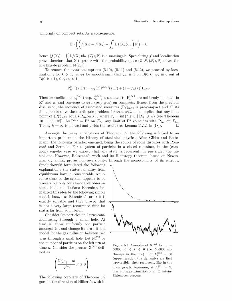
Stochastic differential equations
uniformly on compact sets. As a consequence,
EP
((f(Xt)− f(Xs)−
∫ t
s
Lf(Xu)du
)F
)= 0,
hence (f(Xt)−∫ t
0Lf(Xu)du, (Ft),P) is a martingale. Specializing f and localization
prove therefore that X together with the probability space (Ω,F , (Ft),P) solves themartingale problem M(a, b).
To remove the extra assumptions (5.10), (5.11) and (5.12), we proceed by loca-lization : for k > 1, let ϕk be smooth such that ϕk ≡ 1 on B(0, k) ϕk ≡ 0 out ofB(0, k + 1), 0 6 ϕk 6 1,
P(εn)k (x,Γ) := ϕk(x)P(εn)(x,Γ) + (1− ϕk(x))1x∈Γ.
Then he coefficients a(εn)k (resp. b
(εn)k ) associated to P
(εn)k are uniformly bounded in
Rd and n, and converge to ϕka (resp ϕkb) on compacts. Hence, from the previousdiscussion, the sequence of associated measures (Pnk )n>0 is pre-compact and all itslimit points solve the martingale problem for ϕka, ϕkb. This implies that any limitpoint of (Pnk )n>0 equals PX0
on Fτk where τk = inft > 0 | |Xt| > k (see Theorem
10.1.1 in [18]). As Pn,k = Pn on Fτk , any limit of Pn coincides with PX0 on Fτk .Taking k →∞ is allowed and yields the result (see Lemma 11.1.1 in [18]).
Amongst the many applications of Theorem 5.9, the following is linked to animportant problem in the History of statistical physics. After Gibbs and Boltz-mann, the following paradox emerged, being the source of some disputes with Poin-care and Zermelo. For a system of particles in a closed container, in the (com-mon) ergodic case we expect that any state is recurrent, in particular the ini-tial one. However, Boltzman’s work and its H-entropy theorem, based on Newto-nian dynamics, proves non-reversibility, through the monotonicity of its entropy.
Figure 5.1. Samples of X(m) for m =50000, 0 6 t 6 6 (i.e. 300000 ex-
changes in the urn) : for X(m)0 = 50
(upper graph), the dynamics are firstirreversible, then recurrent, like in the
lower graph, beginning at X(m)0 = 2,
discrete approximation of an Ornstein-Uhlenbeck process.
Smoluchowski formulated the followingexplanation : the states far away fromequilibrium have a considerable recur-rence time, so the system appears to beirreversible only for reasonable observa-tions. Paul and Tatiana Ehrenfest for-malized this idea by the following simplemodel, known as Ehrenfest’s urn : it isexactly solvable and they proved thatit has a very large recurrence time forstates far from equilibrium.
Consider 2m particles, in 2 urns com-municating through a small hole. Attime n, chose uniformly one particleamongst 2m and change its urn : it is amodel for the gaz diffusion between two
urns through a small hole. Let N(m)n be
the number of particles on the left urn attime n. Consider the process X(m) defi-ned as N
(m)bmtc −m√
m, t > 0
.
The following corollary of Theorem 5.9goes in the direction of Hilbert’s wish in
Stochastic differential equations
1900 : Boltzmann’s work on the principles of mechanics suggest the problem of deve-loping mathematically the limiting processes (. . . ) which lead from the atomistic viewto the laws of motion of continua.
Corollary 5.10. Assume that, as m → ∞, N(m)0 −m ∼ α
√m. Then, as m → ∞,
for any finite horizon T > 0, the process (X(m)t , 0 6 t 6 T) converges weakly to the
unique (strong) solution of the Ornstein-Uhlenbeck stochastic differential equationdXt = −Xtdt+ dBt,X0 = α.
Note first that the above continuous limit visits all states, hanks to small fluctua-
tions from the mean in the initial condition : N(m)0 −m ∼ α
√m. If N
(m)0 −m ∼ αm for
some α ∈ (0, 1), then there is no diffusive limit, the way to equilibrium being deter-ministic and non-reversible, the random term is not visible compared to the drift one.On a different topic, the above stochastic differential equation clearly has a uniquestrong solution because its coefficients are Lipschitz, and using the Ito formula thereader can check that the explicit solution is
Xt = e−t(α+
∫ t
0
esdBs
).
Proof. The set of possible values for X(m)t is k√
m,−m 6 k 6 m, and the probability
transitions are
P(m)
(x, x+
1√m
)=
1
2− x
2√m, P(m)
(x, x− 1√
m
)=
1
2+
x
2√m.
As a consequence, with notations analogous to (5.4) and (5.5), a direct calculationyields
b(m)(x) = −x, a(m)(x) = 1.
As condition (5.6) is clearly satisfied and X(m)0 −→
m→∞α, the result follows by the
general Theorem 5.9.
5. Shifts in the Cameron-Martin space
The purpose of this section is to consider stochastic differential equations corres-ponding to shift of the Bownian motion along a predictable element of the Cameron-Martin space :
dXt = dBt + b(Xs, 0 6 s 6 t)dt. (5.13)
By the Girsanov Theorem, we know some properties of any measure weak solution tothis equation : it is absolutely continuous with respect to the Wiener measure, withan explicit density.
A more subtle question concerns the existence/uniqueness of a weak/strong so-lution to this equation. We will show that in the Markovian case, under very weakhypotheses on b, there is a unique strong solution (Zvonkin, [26]). It was conjecturedthat the Markovian hypothesis on b could be relaxed, which was shown to be falsein a famous counterexample due to Tsirelson ([22], see also [25]). Finally, a necessaryand sufficient condition on b for existence/uniqueness of a strong solution to (5.13) isgiven, from the work of Ustunel [24].
5.1. The Zvonkin theorem
Consider a general Markovian differential equation
dXt = σ(Xt)dBt + b(Xt)dt. (5.14)
Stochastic differential equations
A natural idea to study the existence/uniqueness of such an equation consists inchanging the variable, Yt = f(Xt), with f ∈ C 2 : Ito’s formula yields
dYt = (σf ′)(Xt)dBt +
(1
2σ2f ′′ + bs′
)(Xt)dt,
so Y is a local martingale if and only if
1
2σ2f ′′ + bf ′ ≡ 0. (5.15)
Assume that bσ−2 is locally integrable, then
f ′(x) = e−∫ x· 2
b(u)
σ(u)2du
is a solution to (5.15). The function f is strictly increasing, so f−1 is well defined,and Y solves the stochastic differential equation
dYt = s(Yt)dBt (5.16)
with s(x) = (σf ′) f−1. The above stochastic differential equation (and thereforegeneral markovian shifts in the Cameron-Martin space) has a unique weak solution,as shown by the following lemma and delocalization (make ε→ 0 hereafter).
Lemma 5.11. Let s be a measurable function with s(x) > ε > 0. Then (5.16) admitsa unique weak solution, which is a local martingale.
Proof. Let Y be a solution of (5.16). Then its bracket converges to ∞, as
〈Y〉t =
∫ t
0
g(Ys)2ds > εt.
Hence, by the Dubins-Schwarz theorem, β defined by
β〈Y〉t = Yt
is a Brownian motion. More explicitly,
βt = Yτ(t)
where ∫ τ(t)
0
s(Yu)2du = t.
Differentiating the above equation yields
1 = τ ′(t)s(Yτ(t))2 = τ ′(t)s(βt)
2.
This yields an explicit expression of 〈Y〉t in terms of β :
〈Y〉t = infu | τ(u) > t = infu |∫ u
0
τ ′(u)du > t = infu |∫ u
0
du
s(βu)2> t.
Consequently, Y is a continuous function of the Brownian motion β, hence there is aunique possible law for it.
. n.b. : such an f is not necessarily C 2, but this is overcome by IV.45.9 in [17]
Stochastic differential equations
Much better than the above uniqueness in law, strong existence and uniquenesshold under weak assumptions : Zvonkin observed that when σ is Lipschitz, boundedaway from 0, and b only bounded and measurable, the function s in (5.16) is locallyLipschitz, hence there is a unique strong solution to (5.16). As f is invertible, thereis a unique strong solution to (5.14), and in particular to (5.13) where σ ≡ 1 and abounded b depends only on the current point (Markovian case).
By scaling, the above discussion proves that there is always a strong solution to
dYt = εdBt + b(Yt)dt,
no matter how small ε > 0 is. This contrasts with the ordinary differential equation
dYt = b(Yt)dt
which can have several solutions for a bounded measurable b.
5.2. The Tsirelson example
The preceding paragraph contrasts with the following example where b dependson all the past. Note the fractional part
x = x− bxc
and consider the ounded predictable drift
b((Xs)06s6t) =
Xtk−Xtk−1
tk−tk−1
if tk < t 6 tk+1
0 if t = 0,
where (tk)k∈Z is an increasing sequence converging to 0 as k → −∞. Then b isa bounded measurable function, so from the Girsanov theorem for the stochasticdifferential equation
dXt = dBt + b((Xs)06s6t)dt (5.17)
uniqueness in law holds (here (Ω,F , (Ft),P) is a filtered probability space, B is a((Ft),P)-Brownian motion and X is (Ft)-adapted). However, there is no strong so-lution : for any solution X to the above equation, surprisingly for any t > 0 thefractional part (∆X)t of the slope (tk < t 6 tk+1)
(∆X)t :=Xt −Xtk
t− tk
is uniform on [0, 1] and independent of Bs = σ(Bu, 0 6 u 6 s) for any s > 0.
Theorem 5.12. For any t > 0, (∆X)t is uniform on [0, 1] and independent of B∞.Moreover, noting Xt = σ(Xs, s 6 t), for any 0 < s < t
Xt = Bt ∨ σ((∆X)s). (5.18)
Proof. Similarly to (∆X)t, let
(∆B)t =Bt − Btkt− tk
,
for tk < t 6 tk+1. Then, from the stochastic differential equation (5.17), for tk−1 <t 6 tk
(∆X)t = (∆B)t + (∆X)tk−1.
. Example : dYt = 2 sgn(Yt)|Yt|1/2dt has three solutions 0,±t2, due to the bifurcation choice att = 0. Such a phenomena cannot exist in the stochastic case because the Brownian motion preventsfrom making any initial choice.
Stochastic differential equations
This yields, for any p ∈ Z
E(ei2πp(∆X)tk
)= E
(ei2πp((∆B)tk+(∆X)tk−1
))
= E(ei2πp(∆B)tk
)E(ei2πp(∆X)tk−1
)= e− 2π2p2
tk−tk−1 E(ei2πp(∆X)tk−1
),
where we have used the independence between (∆B)tk and Ftk−1: B is a B is a (Ft)-
Brownian motion, hence Bt − Bs is independent of Fs for t > s. An iteration of theabove equality gives for any n > 1 the upper-bound∣∣∣E(ei2πp(∆X)tk
)∣∣∣ 6 e−2π2p2ckn∣∣∣E(ei2πp(∆X)tk−n
)∣∣∣ 6 e−2π2p2ckn,
where ck = inf`6k(t` − t`−1)−1 > 0. This proves that for any p ∈ Z∗ and k ∈ Z
E(ei2πp(∆X)tk
)= 0,
i.e. (∆X)tk is uniform on [0, 1]. Moreover, for any tk < t < tk+1, (∆X)t =(∆B)t + (∆X)tk, where the last term was just proven to be uniform on [0, 1], andis independent of (∆B)t, hence (∆X)t is uniform on [0, 1] for any t > 0.
Now note Buv = σ(Bs, u 6 s 6 v), 0 < u < v. For any v > 0, p ∈ Z,
E(ei2πp(∆X)t | Bv
)= limn→−∞
E(ei2πp(∆X)t | Btnv
),
and this last term vanishes : for sufficiently large n, tn < tk < t 6 tk+1 and supposingt < v,
E(ei2πp(∆X)t | Btnv
)= E
(ei2πp((∆X)tn+(∆B)tn+1
+···+(∆B)tk+(∆B)t) | Btnv)
= ei2πp((∆B)tn+1+···+(∆B)tk+···+(∆B)t) E
(ei2πp(∆X)tn | Btnv
)= ei2πp((∆B)tn+1
+···+(∆B)tk+···+(∆B)t) E(ei2πp(∆X)tn
)where the last equality relies on the independence of Btnv and Ftn . We proved that
E(ei2πp(∆X)tn
)= 0 for p ∈ Z∗, hence if 0 < t < v
E(ei2πp(∆X)t | Bv
)= 0,
which concludes the proof that (∆X)t is independent of Bv whenever v > t, henceindependent of any Bv, v > 0.
Finally, to show that (∆X)s is exactly the missing information to get X fromB, i.e. (5.18), we proceed by double inclusion.
First, from the stochastic differential equation (5.17), B is a functional of X soBt ⊂ Xt. Obviously σ((∆X)s) ⊂ Xt (s < t), so
σ((∆X)s) ∨ Bt ⊂ Xt.
Concerning the other inclusion, we make the observation that (b(Xu), 0 6 u 6 t)is a function of (Bu)06u6t and (∆X)s for any choice of 0 < s < t. Indeed, iftk < s 6 tk+1,
(∆X)s = (∆B)s + (∆X)tk,
so (∆X)tk ∈ σ((∆X)s) ∨ Bs (n.b. : a− b = a − b). Moreover,
(∆X)tk = (∆B)tk + (∆X)tk−1,
Stochastic differential equations
so (∆X)tk−1σ((∆X)tk)∨Btk ⊂ σ((∆X)s)∨Bs, and by induction any (∆X)tn,
n 6 k, is σ((∆X)s)∨Bs-measurable. Proving the measurability of the drifts for t > sis also straightforward :
(∆X)tk+1 = (∆X)tk+ (∆B)tk+1
∈ σ((∆X)tk) ∨ Btk+1,
so by an immediate induction for any n with tn < t, (∆X)tn ∈ σ((∆X)s) ∨ Bt.By going below and up s, we proved that, for any u < t, b((Xv)06v6u) is alwaysσ((∆X)s) ∨ Bt-measurable, hence for u < t
Xu =
∫ u
0
b((Xy)06y6v)dv + Bu ∈ σ((∆X)s) ∨ Bt
which concludes the proof.
5.3. Energy, entropy.
A simple characterization of the existence of a strong solution to
dXt = dBt + utdt, (5.19)
where ut ∈ Xt = σ(Xs, s 6 t), was given in [24]. We abbreviate the above equationas B = (Id − u)X and wonder about P-almost sure invertibility of Id − u. To avoidintegrability problems, we assume that ut is uniformly bounded in ω and t. Notethat by the Girsanov theorem the law R of X is uniquely determined and absolutelycontinuous with respect to that of B. Hence the P-almost sure and R-almost sureinvertibility conditions are the same, so for notational convenience we will considerthe equation
X = (Id− u)B
instead (for the same function u, where ut ∈ Bt = σ(Bs, s 6 t) now), and wonderabout its P-almost sure invertibility. From the above equation, it follows that
Xt ⊂ Bt ⊂ F t .
As previously, (Ω,F , (Ft),P) is a filtered probability space, B is a ((Ft),P)-Brownian motion and X is (Ft)-adapted. Moreover, we consider the context of afinite horizon (0, 1). Let
Lt =dQdP
∣∣∣∣Ft
= EP(L1 | Ft), Q = (Id− u)P,
and we will abbreviate L for L1. By the Ito representation theorem, Lt = ρ(−δyt) for
some F-adapted y,∫ t
0y2sds <∞ a.s., with the notation
ρ(−δyt) = e−∫ t0ysdBs− 1
2
∫ t0y2sds.
Indeed, the Ito representation yields Lt = 1 +∫ t
0αsdBs for some adapted α, and as
Ls > 0 a.s., this can be written
dLt =
(αsLs
)LsdBs,
so L is an exponential martingale.
Theorem 5.13. The application Id − u is P-almost surely invertible, with inverseId + y, if and only if
EP(L log L) =1
2EP
(‖u‖2H
).
Stochastic differential equations
Remark. The above equation means that the relative entropy H(Q | P) coincides withthe kinetic energy of u. The following proof yields to the unconditional inequality
H(Q | P) 61
2EP
(‖u‖2H
).
As entropy measures the number of accessible states, the theorem means that theapplication is invertible if and only if it has just enough energy to fulfill the accessiblestates.
Proof. Assume first that EP(L log L) = 12 EP
(‖u‖2H
). By substitutions,
EP(L log L) = EQ(log L) = EQ(−∫ 1
0
ysdBs −1
2
∫ 1
0
y2sds)
= EQ(−∫ 1
0
ys(ysds+ dBs) +1
2EQ(
∫ t
0
y2sds).
From the Girsanov theorem, (Bs +∫ s
0ysds)s>0 is a (F ,Q)-Brownian motion. As ys is
Fs-adapted, this implies that EQ(−∫ 1
0ys(ysds+ dBs) = 0, so
EP(L log L) =1
2EQ(‖y‖2H) =
1
2
∫‖y‖2H
d(Id− u)P
dPdP
=1
2
∫‖y(ω)‖2HP((Id− u)−1(dω)) =
1
2EP(|y (Id− u)|2H).
Moreover, as X represents LdP, from Lemma 5.14, ys(Id−u) = EP(us | Xs) ds×dP-a.s., so
EP(L log L) =1
2EP
(∫ 1
0
(EP(us | Xs))2ds
),
and using the hypothesis
EP
(∫ 1
0
u2sds
)= EP
(∫ 1
0
(EP(us | Xs))2ds
),
which easily implies
EP
(∫ 1
0
(us − EP(us | Xs))2ds
)= 0,
i.e. us = EP(us | Xs dt× dP almost surely. Hence
ys (Id− u) = us
dt× dP a.s. which means that Id + y is the almost sure inverse of Id− u.
Lemma 5.14. Keeping the previous notations, in particular
Lt =d(Id− u)P
dP|Ft= ρ(−δyt) = e−
∫ t0ysdBs− 1
2
∫ t0y2sds,
then ys (Id− u) = EP(us | Xs) ds× dP-almost surely.
Proof. An easy substitution yields
Lt (Id− u) = e−∫ t0
(ys(Id−u))(dBs+usds+12 ys(Id−u)ds). (5.20)
On the other hand, applications of the Girsanov theorem yield the following expres-sions.
Stochastic differential equations
• First,(Lt (Id− u))E(ρ(−δut) | Xt) = 1. (5.21)
Indeed, for any Ft-measurable f , from the Girsanov theorem,
E(f (Id− u)Lt (Id− u)ρ(−δut)
)= E(fLt) = E(f (Id− u)),
where the last equality just translates Lt = d(Id−u)PdP |Ft . Hence
E(f (Id− u)
(f (Id− u)Lt (Id− u)E(ρ(−δut) | Xt)− 1
))= 0.
We have B := E(ρ(−δut) | Xt) ∈ Xt and the above equation means E(AB) = 0for any A ∈ Xt, so B = 0 P-a.s., proving (5.21).
• Moreover, defining Z by Xt = Zt +∫ t
0E(us | Xs)ds,
E(ρ(−δu) | Xt) = e−∫ t0E(us|Xs)dZs− 1
2
∫ t0E(us|Xs)2ds(=: `t) (5.22)
, by a double application of the Girsanov theorem :
E(f (Id− u)ρ(−δu)) = E(f) = E(f (Id− u)`1),
the last equality relying on the fact that Z is a X -Brownian motion (it is aX -martingale with bracket 〈Z〉t = t). In the above equality, conditioning on Xtimplies the expected result (5.22).
Gathering (5.20), (5.21) and (5.22) yields
1 = (Lt (Id− u))E(ρ(−δut) | Xt)
= e−∫ t0
(ys(Id−u))(dBs+usds+12 ys(Id−u)ds)e−
∫ t0E(us|Xs)dZs− 1
2
∫ t0E(us|Xs)2ds.
Make he substitution dZt = dBt+(us−E(us | Xs))ds in the above formula shows thata continuous semimartingale vanishes almost surely for any t > 0, hence its bracketis 0, which means ys (Id− u) = EP(us | Xs) dt× dP almost surely.

Chapter 6
Representations
1. The Ito representation
2. The Gross-Sobolev derivative
3. The Clark formula
4. The Ornstein-Uhlenbeck semigroup

Chapter 7
Concentration of measure
Obtaining sub-gaussian tails for probability measures, like
P(|X− E(X)| > δ) 6 Ce−cδ2
, (7.1)
is an important goal and tool, making it possible to quantify fluctuations of a randomvariable around its mean. For instance, for random variables depending on an indexn (often the dimension), this allows to bound the variance and therefore to provetightness, which is an important step towards convergence in law.
To motivate our study and understand the nature of concentration results (highdimension, small fluctuations around the mean), we consider in this introduction someexamples proved in the following sections. First, let σ be the uniform probabilitymeasure on the unit sphere S (n) ⊂ Rn+1, and S a subset of S (n) such that µ(n)(S) >1/2. Consider the neighborhood
Sε = x ∈ S (n) | dist(x,S) 6 ε, (7.2)
where dist is the geodesic distance on the sphere. Then
σ(Sε) > 1− e−(n−1)ε2
2 . (7.3)
In particular, as n→∞ the uniform measure gets concentrated in a belt around theequator. This result (7.3) can be shown by first proving that the minimum of σ(Sε)is obtained for an hemisphere, and then by a direct integration. The intuition behindthis last step is that a unit vector of Rn has typical amplitude O(1/
√n) for the nth
coordinate, so the volume of the neighborhood will be close to 1 if nε2 1.Concerning the first step, this isoperimetry result holds for all compact manifold
with strictly positive Ricci curvature, as shown by Gromov, Levy. More precisely, letM be a compact manifold with Riemannian metric g and Riemannian probabilitymeasure µ. Let R(M ) be the infimum of Ric(u, u), over all unit tangent vectors u on
M , and assume R(M ) > 0. For some r > 0, R(M ) = R(S n(r)), where S (n)(r) isa Euclidean sphere of dimension n and radius r, with uniform probability measurenoted σr. Then, if some Borell subsets M ⊂ M , S ⊂ S , have the same measure(µ(E) = σr(S)),
µ(Mε) > σr(Sε),
for any ε > 0. Note that, by the Minkowski content formula, this implies that thelength of the border ∂M is greater than ∂S : this is an isoperimetry result.
As σr(Sε) can be easily estimated, we get that for any ε > 0, if µ(M) > 1/2, forsome absolute constant c,C > 0
µ(Mε) > 1− Ce−cRε2
. (7.4)
We will directly prove such results for any Lipschiz function F by using stochasticanalysis tools, regardless isoperimetry considerations.
. for a Riemannian manifoldM with metric g, the geodesic distance allows to define a neighborhoodMε of M ⊂M up to distance ε in the same way as (7.2). in this chapter, the Lipschitz constant ‖F‖L of a Lipschitz function F : Rn → R is defined with
respect to the Euclidean norm : for all x, y in Rn, |F(x)− F(y)| 6 ‖F‖L|x− y|L2(Rn)
Concentration of measure
Theorem 7.1. For some C, c > 0, independent of the manifold M and the functionF with Lipschitz constant (with respect to the Riemanian metric) ‖F‖L
µ |F− Eµ(F) > ε| 6 Ce−cR(M ) ε2
‖F‖2L .
There are two interesting regimes for these results. For ε → 0, this can yield iso-perimetric estimates like (7.3). For ε > 0, as the dimension increases, this often yields
concentration, because the curvature of the sphere S (n), with radius 1, is R = n− 1.Note that Theorem 7.1 easily implies (7.4), by choosing F(x) = min(dist(x,M), ε).
Bounds like (7.1) or more specifically (7.3) are called concentration inequalities,and many general criteria allow to prove them. Our aim consists in giving a non-exhaustive (see [10] for a review of the concentration phenomenon) description ofsufficient conditions, emphasizing on how, quite surprisingly, some stochastic processesallow to prove these time-independent relations. For example, concentration yields agood understanding of the maximum of any Gaussian process, at first order.
Theorem 7.2. Let g(t)t∈E be a centered Gaussian process indexed by a countable setE, and such that supE g(t) <∞ almost surely. Then E(supE g(t)) <∞ and for everyδ > 0
P(| sup
Eg(t)− E(sup
Eg(t))| > δ
)6 2e−
δ2
2σ2 ,
where σ2 is the maximum of the variances , supE E(g(t)2).
As we will see, this result by Borell is for example a consequence of the hypercon-tractivity of the Ornstein-Uhlenbeck semigroup.
Going to the discrete setting, hypercontractivity is an important tool in computerscience for example. Consider the state space −1, 1d endowed with the uniformprobability measure. To a function f : −1, 1d → −1, 1 (f can be thought as adecision, function of d individual behaviors) one associates the function, Tρf equalat point x to E(f(u)), where u is obtained from x by independently flipping each
bit with probability 1−ρ2 : Tρ is called the noise operator, and is an analogue of the
Ornstein-Uhlenbeck semigroup. Then this semigroup satisfies an hypercontrativityproperty, which is fundamental in the proof of the following famous result with fromKahn, Kanal, Linial [8] (the slightly stronger version stated here comes from Talagrand[20]).
For x = (x1, . . . , xd) ∈ −1, 1d, define the influence of individual i as the proba-bility that changing xi changes f . Let −i for the vector of size n − 1 obtained from(1, . . . , d) by removing the ith coordinate, and ES the expectation with respect to theuniform measures for coordinates in S ⊂ J1, dK,
infli(f) = E−i vari(f).
Then, an easy calculation proves that
d∑i=1
infli(f) > var(f).
Indeed, one naturally expects that the influence of each coordinate on f will be of order1/n times the variance. The remarkable result from [8] is that for some individuals,
the influence goes till log dd times the variance.
. That σ2 <∞ is an easy consequence of E(supE g(t)) <∞. e.g. f(x1, . . . , xd) = x1 is called the dictatorship case, f(x1, . . . , xd) = x1 . . . xd is the parity, and
f(x1, . . . , xd) = sgn(x1 + · · ·+ xd) is the majority.. Think about ρ = e−t, with t a time, so that T1f = f and T0f = E(f) are natural
Concentration of measure
Theorem 7.3. Under the above assumptions, thee is a constant c > 0 not dependingon d such that for any Boolean function f
d∑k=1
inflk(f)
− log inflk(f)> c var(f).
This statement allows to give a framework for sentences like 3% of the populationcan decide about the ending of the vote with probability 99%. Of course, the proofwill not be constructive, so gives no clues about how to find this precious samplingamongst the coordinates. In the proof we will give, the noise operator is useful becauseit improves integrability (hypercontractivity) but also because Tρf very explicit interms of f , when this function is expanded on a Fourier basis. This is very similar tothe use of the Ornstein-Uhlenbeck semigroup to prove continuity of chaos in Lp, seeChapter 6.
This chapter only gives a partial view of concentration results. Another aspect Iparticularly like (but we won’t treat in this class) is the Talagrand inequalities [21].They allow for example to prove this visual example of concentration, given by Taoand Vu [19], which is an important tool in Random Matrix Theory.
Theorem 7.4. Let X1, . . . ,Xn be i.i.d. centered Bernoulli random variables, X =(X1, . . . ,Xn), and V a given subspace of Rn of dimension d. Then
P(|dist(X,V)−√n− d| > δ) 6 Ce−cδ
2
,
for some constants C and c independent of n and d.
The above result means that the typical distance between a random element ofthe hypercube and a subspace of dimension d is
√n− d, with small (concentrated
with no normalization) deviations from the mean.
1. Hypercontractivity, logarithmic Sobolev inequalities and concentration
1.1. Diffusion semigroups
On Rd endowed with a measure µ, consider a family of operators (Pt)t>0 actingon bounded measurable functions through a transition kernel
Pt f(x) =
∫Rdf(y)pt(x,dy),
the measures pt(x, ·) being bounded and positive, t > 0. We will only consider casesin which the domain of Pt can be extended to L2(µ) : ‖Ptf‖L2(µ) 6 c(t)‖f‖L2(µ). Weare interested in the case of continuous semigroups, meaning :
• the semigroup property : Pt Ps = Pt+s, s, t > 0 ;
• the continuity in L2(µ) : for all f ∈ L2(µ), as t→ 0,
Pt f −→L2(µ)
f.
Moreover, if Pt 1 = 1 for any t > 0 (Markovian semigroup), there exists a Markovprocess (Xt)t>0 such that
Pt f(x) = E (f(Xt) | X0 = x) .
. P(X1 = 1) = 1/2, P(X1 = −1) = 1/2. Cf the Hille-Yoshida theorem
Concentration of measure
Definition 7.5. The domain D2(L) ⊂ L2(µ) is the set of functions f ∈ L2(µ) suchthat the limit
L f := limt→0
Pt f − ft
exists in L2(µ). Then D2(L) is dense in L2(µ) and L characterizes the semigroup :
∂t Pt f = L Pt f = Pt L f.
The semigroup (Pt)t>0 is said to be a diffusion semigroup if for any f1, . . . , fn in thedomain and Φ : Rn → R in C∞
L Φ(f1, . . . , fn) =∑i
∂xiΦ(f1, . . . , fn) L fi +∑i,j
∂xixj (f1, . . . , fn)Γ1(fi, fj),
where Γ1(f, g) = 12 (L(fg)− f L g − g L f) is the operator carre du champ.
The measure µ is said to be invariant by (Pt)t>0 if for any f ∈ L1(µ), t > 0,∫Pt fdµ =
∫fdµ.
The measure µ is said to be reversible by (Pt)t>0 if for any f, g ∈ L1(µ), t > 0∫(Pt f)gdµ =
∫g(Pt f)dµ.
Note that, for Markovian semigroups, the reversibility implies the invariance. Mo-reover, for a diffusion semigroup, L(1) = 0, so the semigroup is Markovian.
1.2. Logarithmic Sobolev inequalities
The Sobolev inequality bounds the fluctuations of a function in terms of itsderivative, and therefore can somehow yield to some concentration. For example,any compactly supported smooth function f : Rn → R, if f ∈ Lp(Rn,dx) and∂xif ∈ Lp(Rn,dx), 1 6 i 6 n, then f ∈ Lp∗(Rn,dx) and
‖f‖p∗ 6 c(n, p)‖∇f‖p, (7.5)
where 1 6 p < n, p∗ = npn−p > p : a Sobolev inequality provides an improved inte-
grability on f in terms of that of its derivative. In probabilistic terms, this allows forexample to bound a variance in terms of the Lipschitz constant. One may want toquantify the fluctuations of the function in terms of its gradient in a dimensionlessinequality, which cannot be achieved in (7.5) (e.g. p∗ → p as n→∞, hence it doesn’tgive additional integrability on f).
General concentration estimates, of type (7.1), can be obtained as a corollary ofthe following logarithmic analogue of (7.5).
Definition 7.6. A measure µ on some space X is said to satisfy a logarithmicSobolev inequality with constant c > 0 if for any non-negative f
Eµ(f2 log(f2)
)− Eµ
(f2)
logEµ(f2)6 cEµ
(|∇f |2
).
Here, the definition of ∇f depends on the context and its modulus is considered as ∞in the non-differentiable case.
We will see later general very efficient criteria on µ for satisfying this generalinequality. The above-stated logarithmic Sobolev inequality, corresponding to p = 2,implies analogues for any p > 2.
. In this course X will be either a Riemannian manifold or −1, 1n.
Concentration of measure
Lemma 7.7. Let (Pt)t>0 be a diffusion semigroup with invariant measure µ. Assumethat µ satisfies a logarithmic Sobolev inequality with constant c.
Then for any p > 2 and any positive function f ∈ D
Eµ (fp log(fp))− Eµ (fp) logEµ (fp) 6 −c p2
4(p− 1)Eµ(fp−1 L f
).
Proof. If (Pt)t>0 is a diffusion semigroup, then
p2
4(p− 1)Eµ(fp−1 L f
)= −p
2
4Eµ(fp−2Γ1(f)
)= −p
2Eµ(fp2−1Γ1(f, fp/2)
)= −p
2Eµ(
Γ1(fp2 ))
p2
4(p− 1)Eµ(fp−1 L f
)= Eµ
(fp2 L f
p2
),
hence the expected result is the logarithmic Sobolev inequality applied to the functionfp2 .
An interesting feature of logarihmic Sobolev inequalities is that they tensorize, inthe following way. This will be useful in Section 4. To state this property, given afunction f on X = X1 × · · · ×Xd, note
fi(xi) = f(x1, . . . , xn),
the function fi depending on the frozen coordinates x1, . . . , xi−1, xi+1, dots, xd.
Proposition 7.8. Assume that for any 1 6 k 6 d the measure µk on Xk satisfies alogarithmic Sobolev inequality with constant ck : for any non-negative function h
Entµk(h2) 6 ck
∫Xk
|∇kh|2dµk.
Then µ = µ1 ⊗ · · · ⊗ µk satisfies a logarithmic Sobolev inequality with constant c =max16k6d ck : for any non-negative function f on X
Entµ(f2) 6 c
∫X
|∇f |2dµ,
where |∇f |2 is defined as∑dk=1 |∇kfk|2.
Proof. The statement easily follows from the inequality
Entµ(f) 6∫ d∑
k=1
Entµk(fk)dµ, (7.6)
that we will prove by an extremal characterization of the entropy :
Entµ(f) = sup∫fhdµ |
∫ehdµ 6 1. (7.7)
. we know that for diffusion semigroups
Γ1(F(f), g) = F′(f)Γ1(f, g), Eµ(F′(f) L f) + Eµ(F′′(f)Γ1(f)) = 0.
. Here, as in Definition 7.6, the definition of the gradient is arbitrary/depending on the context
and has no influence on the conclusion of the proposition
Concentration of measure
Indeed, first note that we can suppose that∫fdµ = 1 by homogeneity (if λ > 0,
Ent(λf) = λEnt(f)). Then, Young’s inequality (f non-negative and g real) fh 6f log f − f + eh yields, once integrated,∫
fhdµ 6 Entµ(f)− 1 +
∫ehdµ.
This proves that the left hand side of (7.7) is greater than the right side. The reverseinequality is obtained by choosing h = log f . As a consequence of (7.7), a sufficientcondition to prove (7.6) is that if
∫ehdµ 6 1 then∫
fhdµ 6∫ d∑
k=1
Entµk(fk)dµ.
This is true by interpolating between 1 and h in the following way. For 1 6 k 6 n, let
h(k)(xk, . . . , xn) = log
(∫ehdµ1 . . . dµk−1
)− log
(∫ehdµ1 . . . dµk
).
Then, as∫ehdµ 6 1,
∑dk=1 h
(k) > h. Moreover, obviously∫eh
(k)k dµk = 1. Hence∫
fhdµ 6d∑k=1
∫fh(k)dµ =
d∑k=1
∫ (∫fkh
(k)k dµk
)dµ 6
∫ d∑k=1
Entµk(fk)dµ,
as expected.
1.3. Herbst’s lemma
The link between Logarithmic Sobolev inequalities and concentration lies in thefollowing Lemma, by Herbst.
Lemma 7.9. Assume that µ satisfies a logarithmic Sobolev inequality on Rn withconstant c. Let F : Rn → R be a Lipschiz function, with Lipschitz constant ‖F‖L.Then, for any λ ∈ R,
Eµ(eλ(F−Eµ(F))
)6 ecλ
2‖F‖2L/4. (7.8)
In particular, for any δ > 0,
µ |F− Eµ(F)| > δ 6 2e− δ2
c‖F‖2L . (7.9)
Proof. First note that (7.9) is a consequence of (7.8) : for any λ > 0, by the Bienayme-Chebyshev inequality,
µ |F− Eµ(F)| > δ 6 e−λδ Eµ(eλ|F−Eµ(F)|
)6 e−λδ
(Eµ(eλ(F−Eµ(F))
)+ Eµ
(e−λ(F−Eµ(F))
))6 2e−λδecλ
2‖F‖2L/4.
The optimal choice λ = 2δc‖F‖2L
yields (7.9).
To prove (7.8), assume first that F is differentiable, with uniformly bounded deri-vatives :
‖F‖L = supx∈Rn‖∇F‖L2(x) <∞.
Moreover, we can suppose Eµ(F) = 0. Let f(λ) = log‖e2F‖Lλ , λ > 0. Then a directcalculation yields
d
dλf(λ) =
1
λ2
Eµ(2λFe2λF)− Eµ(e2λF) logEµ(e2λF)
Eµ(e2λF),
Concentration of measure
which is bounded by the logarithmic Sobolev inequality by
cEµ(‖∇eλF‖2L2)
λ2 Eµ(e2λF)6 c sup
Rn‖∇F‖2L2 .
Moreover, as Eµ(F) = 0, limλ→0+ f(λ) = 0, hence f(λ) 6 λc supRn‖∇F‖2L2 for allλ > 0, which is the expected result. If λ < 0, the same result holds by considering−F.
If F is not differentiable with uniformly bounded derivatives, then we proceed byapproximation :
• We note, for ε > 0, Fε(x) = F(x) if −1/ε < F(x) < 1/ε, −1/ε if F(x) < ε and
1/ε if F(x) > −1/ε. Noting pε the Gaussian density pε(x) = e−|x|22ε /(2πε)n/2,
and the convolution Fε(x) = pε ?F, then Fε(x) converges simply to F (|Fε(x)−F(x)| 6 ‖F‖L
√εn), it is continuously differentiable and we will be able to apply
the above discussion to it.
• Indeed, the gradient of Fε(x) is uniformly bounded : it is an easy exercise thatsupRn‖∇Fε‖L2 < ‖F‖L, thus from the differentiable case, we know that
Eµ(eλFε
)6 eλEµ(Fε)ecλ
2‖F‖2L/4. (7.10)
• Thanks to the simple convergence we can use Fatou’s lemma, and get Eµ(eλF) 6
elim infε→0 λEµ(Gε)ecλ2‖F‖2L/2. Hence the proof will be complete if limε→0 Eµ Fε =
Eµ F.
• From the concentration property of Fε (7.10),
µ|Fε − Eµ(Fε)| > δ 6 Ce−cδ2
,
with C and c independent of ε. Hence Fε−Eµ(Fε) is uniformly integrable. If wecan show that Eµ(Fε) is bounded, it will give the uniform integrability of Fε,hence the expected convergence limε→0 Eµ Fε = Eµ F.
• As Fε converges simply to F, by dominated convergence we can find K, ε0 suchthat, for ε < ε0, µ|Fε| < K > 3/4.
Moreover, from (7.10), for r sufficiently large, µ|Fε − Eµ(Fε)| < r > 3/4.Hence, for ε < ε0, with probability at least 1/2, both |Fε| < K and |Fε −Eµ(Fε)| < r, hence Eµ(Fε) < K + r : this event, has measure 0 or 1, hence it isalmost sure.
1.4. Gross’s Theorem
Definition 7.10. Given a strictly increasing function q : R+ → [q(0),∞), a semi-group (Pt)t>0 is said to be hypercontractive with contraction function q if, for anyf ∈ D and any t > 0,
‖Pt f‖q(t) 6 ‖f‖q(0).
Theorem 7.11 (Gross). Let (Pt)t>0 be a Markov semigroup with invariant measureµ such that either µ is reversible or (Pt)t>0 is a diffusion semigroup.
If (Pt)t>0 is hypercontractive with constant q(t) = 1 + e4tc , c > 0, then µ satisfies
a logarithmic Sobolev inequality with constant c.If µ satisfies a logarithmic Sobolev inequality with a constant c > 0, then for any
q(0) > 1 and q(t) = 1 + (q(0) − 1)e4tc , (Pt)t>0 is hypercontractive with contraction
function q.
Concentration of measure
Proof. The proof relies on the differentiation with respect to t,
d
dtlog‖Pt f‖q(t) =
q′(t)
q(t)2 Eµ((Pt f)q(t)
) (∫ (Pt f)q(t) log((Pt f)q(t))dµ
−∫
(Pt f)q(t)dµ log
(∫(Pt f)q(t)dµ
)+q(t)2
q′(t)Eµ(
(Pt f)q(t)−1 L Pt f))
. (7.11)
Suppose first that (Pt)t>0 is hypercontractive with contraction function q(t) =
1 + e4tc :
‖Pt f‖q(t) 6 ‖P0 f‖q(0),
hence the derivative of t 7→ log‖Pt f‖q(t) is negative at 0. From the above differentia-
tion, and as q(0)2/q′(0) = c, this means∫f2 log(f2)dµ−
∫f2dµ log
(∫f2dµ
)6 −c
∫f L fdµ,
which is the expected logarithmic Sobolev inequality.If µ satisfies a logarithmic Sobolev inequality, with constant c > 0, then Lemma
7.7 applied to Pt f yields∫(Pt f)q(t) log((Pt f)q(t))dµ−
∫(Pt f)q(t)dµ log
(∫(Pt f)q(t)dµ
)6 −c q(t)2
4(q(t)− 1)
∫(Pt f)q(t)−1 L Pt fdµ.
For our choice q(t) = 1 + (q(0)− 1)e4t/c,
cq(t)2
4(q(t)− 1)=q(t)2
q′(t),
hence from the differentiation (7.11) the function t 7→ log‖Pt f‖q(t) is decreasing,which means the expected hypercontractivity.
2. Concentration on Euclidean spaces
2.1. Concentration for the extremum of Gaussian processes.
We are now in position to prove Borell’s inequality.
Theorem 7.12. Let g(t)t∈E be a centered Gaussian process indexed by a countableset E, and such that supE g(t) < ∞ almost surely. Then E(supE g(t)) < ∞ and forevery δ > 0
P(| sup
Eg(t)− E(sup
Eg(t))| > δ
)6 2e−
δ2
2σ2 ,
where σ2 is the maximum of the variances , supE E(g(t)2).
Proof. Consider the Gaussian probability measure
dµ =1
Zne−V(x)dx =
1
(2π)n/2e−∑nk=1
x2k2 dx1 . . . dxn
on Rn. Obviously, Hess(V) > Idn, so µ satisfies a Logarithmic Sobolev inequality withconstant 2, by the Bakry-Emery Theorem 7.13. Now, consider a finite set of points
. That σ2 <∞ is an easy consequence of E(supE g(t)) <∞
Concentration of measure
t1, . . . , tn in E, and the Gaussian vector g = (g(t1), . . . , g(tn)), with covariance tVV :
glaw= Vx where x is a vector of standard centered Gaussians.Consider x→ sup16i6n(Vx)i. This is a Lipschiz function with constant σ :
|F(x)− F(y)| 6 sup16i6n
|(Vx)i − (Vy)i| = |n∑j=1
Vij(xj − yj)|
6
√√√√ n∑j=1
V2i,j |x− y|L2 =
√var(g(ti))|x− y|L2 6 σ|x− y|L2 .
Consequently, we can apply Herbst’s Lemma 7.9 and get
P(∣∣∣∣ sup
16k6ng(tk)− E( sup
16k6ng(tk))
∣∣∣∣ > δ
)6 e−
δ2
2σ2 . (7.12)
Note that this upper bound does not depend on n, which makes us confident inextending the result to a countable set T. We can achieve this in the following way.
First, E(supT g(t)) < ∞. Indeed, let Tn be a finite subset of T. Then for anya, b > 0,
E(supTn
g(t)) < a+ b ⊃ supTn
g(t) > E(supTn
g(t))− a ∩ supTg(t) < b.
From (7.12), for a large enough (and not depending on n), the first event has pro-bability 3/4, and the second has probability at least 3/4 for b large enough, assupT g(t) < ∞ almost surely. E(supTn g(t)) is shorter than a + b with probability1/2, thus with probability 1. Now, taking increasing subsets Tn → T (possible, as Tis countable), by monotone convergence E(supT g(t)) <∞.
To conclude, by dominated convergence, for an increasing sequence of subsetsTn → T and r > 0, by (7.12)
P(supTg(t)− E(sup
Tg(t)) > r) = lim
n→∞P(sup
Tn
g(t)− E(supTg(t)) > r) 6 e−
δ2
2σ2
where δ = r + |E(supT g(t))− E(supTn g(t))|. For n→∞, δ → r as previously seen,by monotone convergence. This concludes the proof, applying the same method forthe lower bound.
Theorem 7.12 can be applied to Gaussian processes indexed by an interval un-der the continuity assumption (continuity obtained e.g. by Kolmogorov’s regularity
criterion). Note that for the Brownian motion on [0, 1], σ = 1 and sup g(t)law= |X|,
X ∼ N (0, 1), so
logP (| sup g(t)− E(sup g(t))| > δ) ∼δ→∞
−δ2
2,
coherent with the Theorem 7.12. However, for more general covariance structures,this theorem is one of the very few general bounds on the law of extremes. It yieldsthe exact first order queuing probability for the maximum :
logP (sup g(t) > δ) ∼δ→∞
− δ2
2σ2.
To prove the above estimate, of large deviations type, the upper bound is a straight-forward consequence of Theorem 7.12, and the lower bound follows from
logP(sup g(t) > δ) > logP(g(s) > δ) ∼δ→∞
− δ2
2σ2s
,
noting σs = var(g(s)), and considering the supremum over the σs’s.
Concentration of measure
2.2. Convex potentials
Theorem 7.13 (Bakry, Emery). Assume that the potential V : Rn → R is strictlyconvex, in the sense that for some c > 0
Hess(V) >1
cId, (7.13)
for the partial order of symmetric operators. Then the probability measure
µ =1
Zne−V(x1,...,xn)dx1 . . . dxn
satisfies the logarithmic Sobolev inequality with constant 2c, i.e. for any differentiablefunction f : Rn → R∗+∫
f log fdµ−(∫
fdµ
)(log
∫fdµ
)6 2c
∫|∇√f |2dµ.
Proof. The idea consists in integrating along the semigroup (Pt)t>0 associated with
the invariant measure e−V
Zn:∫
f log fdµ−∫fdµ log
∫fdµ = F(0)− F(∞)
where F(t) =∫
Pt f log Pt fdµ. That F(∞) =∫fdµ log
∫fdµ follows from the ergo-
dicity result Lemma 7.14 (we can assume that f has bounded derivatives and that itsimage is included in a compact of R∗+ and conclude by dominated convergence).
We need to control the derivative
F′(t) =
∫ ((d
dtPt f
)log Pt f +
d
dtPt f
)dµ.
The second term makes no contribution because∫∫∞
0ddt Pt fdµdt =
∫(f−
∫fdµ)dµ =
0, still by ergodicity. The first term is∫(L Pt f) log Pt fdµ = −
∫Γ1(Pt f, log Pt f)dµ = −
∫Γ1(Pt f)
Pt fdµ,
where we used∫f(L g) = −
∫Γ1(f, g) in the first equality. From Lemma 7.15, this is
greater than
−e− 2tc
∫(Pt
√Γ1(f))2
Pt fdµ.
Now, by the Cauchy-Schwarz inequality, for any positive functions a and b,
(Pt a)2
Pt b=
(Pt
(a√b
√b))2
Pt b6 Pt
(a2
b
),
so finally
F′(t) > −e− 2tc
∫Pt
(Γ1(f)
f
)dµ = −e− 2t
c
∫Γ1(f)
fdµ.
Integrating yields F(0)− F(∞) 6 2c∫|∇√f |2dµ, as expected.
Lemma 7.14. If the curvature condition (7.13) holds, then the semigroup (Pt)t>0
is ergodic, in the sense that for any bounded Lipschitz f ∈ D , almost surely (for theLebesgue measure)
Pt f −→t→∞
∫fdµ.
Concentration of measure
Proof. For given initial data and t > 0, let
ϕ(s) = Ps(Γ1(Pt−s f)).
Then
ϕ′(s) = Ps(L Γ1(Pt−s f)) + 2 Ps(Γ1(Pt−s f,L Pt−s f)) = 2 Ps Γ2(Pt−s f). (7.14)
By the curvature condition (7.13), this is bounded by 2c Ps Γ1(Pt−s f), hence ϕ′(s) 6
2cϕ(s), so by Gronwall’s lemma ϕ(t) > ϕ(0)e
2c t, i.e.
Γ1(Pt f) 6 e−2c t Pt Γ1(f). (7.15)
As f is Lipschitz, Γ1(f) is uniformly bounded in space, so Pt Γ1(f) is uniformlybounded in space and time, so Γ1(Pt f) converges uniformly to 0 in Rn. HencePt f converges to a constant, uniformly on compact sets (|Pt f(x) − Pt f(y)| 6|√
Γ1(Pt f)|∞|x−y|). Moreover, for any ε > 0 and x ∈ Rn there is a compact K ⊂ Rnsuch that x ∈ K, µ(K) > 1− ε, so
|Pt f(x)−∫fdµ| 6
∫|Pt f(x)−Pt f(y)|dµ(y) 6 2ε|f |∞+
∫K
|Pt f(x)−Pt f(y)|dµ(y),
and the last integral goes to 0 thanks to the uniform convergence on compacts. Thisconcludes the proof.
Lemma 7.15. If the curvature condition (7.13) holds, then for all f ∈ D√Γ1(Pt f) 6 e−
tc Pt
(√Γ1(f)
).
Proof. Let
ψ(s) = e−sc Ps
√Pt−s f.
Then, noting g = Pt−s f ,
ψ′(s) = −1
cψ(s) + e−
sc Ps
(L√
Γ1(g))− e− sc Ps
(Γ1(g,L g)√
Γ1(g)
).
Moreover, for F : Rn → R and f = (f1, . . . , fn),
L F(f) =∑
(∂iF)fi +∑i,j
(∂ijF)(f)Γ1(fi, fj),
so
L√
Γ1(g) =L Γ1(g)
2√
Γ1(g)− Γ1(Γ1(g))
4Γ1(g)3/2.
This yields
ψ′(s) = e−sc Ps
(L Γ1(g)− 2Γ1(g,L g)
2√
Γ1(g)− Γ1(Γ1(g))
4Γ1(g)3/2− 1
c
√Γ1(g)
)
= e−sc Ps
(4Γ1(g)
(Γ2(g)− 1
cΓ1(g))− Γ1(Γ(1)(g))
4Γ1(g)3/2
).
This is positive thanks to Lemma 7.16, so ψ(t) > ψ(0), as expected.
Lemma 7.16. If the curvature condition (7.13) holds, for any f ∈ D,
4Γ1(f)
(Γ2(f)− 1
cΓ1(f)
)> Γ1(Γ1(f)).
Concentration of measure
Proof. An elementary (and long) differentiation yields, for F : Rn → R, f =(f1, . . . , fn),
Γ2(F(f)) =∑i,j
∂iF(f)∂jF(f)Γ2(fi, fj) + 2∑i,j,k
∂iF(f)∂jkF(f)H(fi)(fj , fk)
+∑i,j,k,l
∂ijF(f)∂klF(f)Γ1(fi, fk)Γ1(fj , fl)
where H(f)(g, h) = 12 (Γ1(g,Γ1(f, h)) + Γ1(h,Γ1(f, g))− Γ1(f,Γ1(g, h))). Applying
this to F such that, at point (f, g)(x0),
∇F =
(10
),Hess F =
(0 xx 0
),
we get
Γ2(F(f, g)) = Γ2(f) + 4xH(f)(f, g) + 2x2(Γ1(f, g)2 − Γ1(f)Γ1(g))
>1
cΓ1(F(f, g)) =
1
cΓ1(f).
The discriminant of this positive binomial needs to be negative, which implies, (byusing H(f)(f, g) = Γ1(Γ1(f), g) and Γ1(f, g)2 6 Γ1(f)Γ1(g))
Γ1(g,Γ1(f))2 6 4
(Γ2(f)− 1
cΓ1(f)
)Γ1(f)Γ1(g),
and the expected result for g = Γ1(f).
3. Concentration on curved spaces
Theorem 7.13 admits a Riemannian analogue, based on the same ideas, and whichonly requires some basis on differential geometry.
Consider M a compact manifold of dimension n with a Riemannian metric g.Then gx is a positive definite bilinear map on the tangent space of M at pointx, Tx(M ). The natural underlying measure, µ, associated with (M , g) is the locallydµ(x) =
√detgxdx. We are interested in whether smooth modifications of this volume
measure satisfy a logarithmic Sobolev inequality. Let
µV(dx) =1
Ze−V(x)dµ(x)
with V a smooth function on M . A stochastic process with invariant measure µV isgiven through its semigroup
Pt = etLV , LV(f) = ∆f − g(∇V,∇f),
where ∆ is the Laplace Beltrami operator on (M , g), i.e. ∆f = div∇f with divX =∑i g(Li, [Li,X]) in local coordinates. Equivalently,∫
g(∇f,X)dµ = −∫fdivXdµ.
Finally, the Riemannian analogues of Γ1 and Γ2 are naturally given by
Γ1(f, h) = g(∇f,∇h),
Γn(f, h) =1
2(LV Γn−1(f, h)− Γn−1(LV f, h)− Γn−1(f,LV h)) .
Additionally to the Hessian of V, a Bakry-Emery type criterium needs to take intoaccount the shape, curvature, of M . This is expressed through the Ricci tensor :
. (Li)16i6n is an orthogonal frame, for the metric g, at point x, and the Lie bracket of two vector
fields, noted [X,Y] = XY −YX, is defined as [X,Y]i =∑nj=1(Xj∂jYi −Yj∂jXi)
Concentration of measure
• A connection is a bilinear operation associating to vector fields X and Y a thirdone, ∇XY, such that for any smooth f
∇fXY = f∇XY, ∇X(fY) = f∇XY + (Xf)Y.
The Levi-Civita connection is the unique torsion-free connection (∇XY−∇YX =[X,Y]) such that Xg(Y,Z) = g(∇XY,Z) + g(Y,∇XZ).
• The Riemann curvature tensor R(,·) associates to vector fields X,Y an operatoron vector fields R(X,Y) defined by (∇ is the Levi-Civita connection)
R(X,Y)Z = ∇X(∇YZ)−∇Y(∇XZ)−∇[X,Y]Z.
• The Ricci curvature tensor associates to vector fields X and Y the functionRic(X,Y), smooth on M , such that for any orthogonal local frame (Li)
Ric(X,Y)(x) =
n∑i=1
gx(R(X,Li)Li,Y).
In more intuitive words, the Ricci cirvature measures the first non-trivial orderof difference between the Riemannian metric and its Eucliden approximation :in loal geodesic coordinates,
dµ =
(1− 1
6Rjkx
jxk)
dµEuclidean.
The iterated carre du champ operator Γ2 encodes both the Hessian of V and thecurvature, as shown by the Bochner formula, which is a key step in the next theorem :
Γ2(f, f) = 〈Hess f,Hess f〉+ (Ric + Hess V)(∇f,∇f),
where 〈Hess f,Hessh〉 =∑i,j(Hess f)(Li,Lj)(Hessh)(Li,Lj).
Proof of Theorem 7.1. We closely follow the dynamical method of Ledoux [11], in thesame vein as the proof of the Bakry-Emery Thorem 7.13.
First, it is sufficient to show that, for some C, c > 0, for any F with mean Eµ(F) =0,
Eµ(eλF)6 Ce
c λ2
R‖F‖2L . (7.16)
Indeed, like in the proof of the Herst Lemma 7.9, using the Bienayme-Chebyshevinequality,
µ |F− Eµ(F) > u| 6 Ce−λu+c λ2
R‖F‖2L ,
and minimizing over λ (take λ = Ru2c‖F‖2L
) yields the result.
Now, to prove (7.16), we use the Bochner formula, which relates the Ricci curvatureto the Laplace-Beltrami operator, and can be written as
1
2∆(|∇F|2)−∇F · ∇(∆F) = Ric(∇F,∇F) + ‖Hess F‖HS;
Consider the Brownian motion on M , with associated semigroup Pt = et∆, t > 0.Note ϕ(s) = Ps(|∇(Pt−sf)|2). Then, in the same way as (7.14),
ϕ′(s) = Ps(∆Γ1(Pt−s F))− 2 Ps(Γ1(Pt−s F,∆ Pt−s F)) > 2Rϕ(s),
from the Bochner formula. Hence
|∇(Pt F)|2 6 e−2Rt Pt(|∇F|2). (7.17)
Concentration of measure
This estimate will be important in the end of the proof. Let ψ(t) = Eµ(eλPt F). We
want to show that Ψ(0) 6 CeCλ2/R. Note that
ψ′(t) = λEµ(∆(Pt F)eλPt F) = −λ2 Eµ(|∇(PtF)|2eλPt F) > −λ2e−2Rtψ(t).
This easily implies
logψ(0)− logψ(∞) 6∫ ∞
0
λ2e2Rtdt =λ2
2R,
which concludes the proof, noting that by ergodicity ψ(∞) = 1.
Theorem 7.17. Suppose that for any p ∈ M
Ricp +(Hess V)p >1
cgp,
in the sense of partial order of positive operators. Then µV satisfies a logarithmicSobolev inequality with constant 2c. In particular, for any Lipschitz function F (withrespect to the geodesic distance on M ),
PµV (|F− Eµ F| > δ) 6 2e− δ2
c‖F‖2L
4. Concentration and Boolean functions
This section aims to give an idea about why hypercontractivity is an importanttool to quantify influences in discrete complex systems. This applies for example totheoretical computer science and percolation theory (see [5] for a much more completeanalysis).
Let µ be the uniform measure on E = −1, 1d. For S ⊂ J1, dK and x ∈ E, letχS(x) =
∏k∈E xk. These functions are a Fourier basis on L2(E, µ) : for any f : E→ R,
f(x) =∑
S⊂J1,dK f(S)χS(x), where f(S) = E(f(x)χS(x)).
For the Gaussian measure, we first proved hypercontractivity and then the loga-rithmic Sobolev inequality ; the steps will be reversed in the following, concerning theuniform measure on the hypercube.
Given a function f : E → R, let f−k(x) = f(x1, . . . , xk−1,−xk, xk+1, . . . , xd). Wedefine the differential operator as
Dkf(x) =f(x)− f−k(x)
2.
Theorem 7.18. The measure µ satisfies the logarithmic Sobolev inequality withconstant 2, in the sense that for any f : E→ R
Entµ(f2) 6 2
∫E
d∑k=1
|Dkf |2dµ.
Proof. We first prove it for d = 1, which means that for any real a and b
1
2
(a2 log(a2) + b2 log(b2)
)− a2 + b2
2log
a2 + b2
26
(a− b)2
2.
Assume a > b. Writing c = (a+ b)/2 and x = (a− b)/2. We need to prove that
ϕ(x) = (c2 + x2) log(c2 + x2) + 2x2 − (c+ x)2 log(c+ x)− (c− x)2 log(c− x)
is positive. As ϕ(0) = 0, this will follow if ϕ′ > 0 on [0, c). A calculation yields
1
2ϕ′(x) = 2x+ 2x log(c2 + x2)− (c+ x) log(c+ x)− (x− c) log(c− x),
Concentration of measure
which is 0 at x = 0, so we just need ϕ′′ > 0 on [0, c). Annyother calculation gives
1
2ϕ′′(x) =
2x2
c2 + x2+ log
(1 +
2x2
c2 − x2
)> 0,
concluding the proof when d = 1. The general case follows from the tensorizationproperty, Proposition 7.8.
The above result implies hypercontractivity for the following semigroup. Given afunction f : E → R, let Tρf(x) be the expectation of f(y) where y is obtained from
x by flipping each entry of x with probability 1−ρ2 :
Tρf(x) =∑y∈E
f(y)
d∏k=1
(1 + ρ
21yk=xk +
1− ρ2
1yk=−xk
)= E(f(xu)
d∏k=1
(1 + ρuk)).
In particular,
TρχS(x) = E(χS(xu)
d∏k=1
(1 + ρuk)) = χS(x)E(χS(u)
d∏k=1
(1 + ρuk)) = ρ|S|χS(x).
As the χS’s are a basis of L2(E, µ), this proves that (Tρ, 0 6 ρ 6 1) is a semigroup(note that here T1 = Id : ρ needs to be thought of as e−t where t is a time) :Tρ1 ? Tρ1 = Tρ1ρ2 .
The semigroup T is contractive in Lp for p > 1, as an easy consequence of Jensen’sinequality. Like the Ornstein-Uhlenbeck semigroup, thanks to its smoothing propertyit is even hypercontractive.
Theorem 7.19. For any ρ ∈ [0, 1] and 1 6 p 6 q satisfying q 6 1 + ρ−2(p− 1),
‖Tρf‖Lq 6 ‖f‖Lp .
Proof. We proceed like in Gross’s Theorem 7.11, showing that the logarithmic Sobolevinequality Theorem 7.18 implies hypercontractivity for Pt = Te−t . For this, we needto identify the generator of the semigroup Pt. This is easy when looking at the basefunctions :
d
dtPtχs =
d
dte−t|S|χS = −|S|Ptχs,
so Lf = L(∑fSχS) = −
∑|S|fSχS. In particular,
−E(fLf) = E((∑
fSχS
)(∑|S|fSχS
))=∑|S|f2
S .
We need to prove that this coincides with E(∑
k |Dkf |2). For this, note that
DkχS = 1k∈SχS,
so
E
(∑k
|Dkf |2)
=∑k
∑S
1k∈Sf2S =
∑|S|f2
S ,
as expected.
We are now in a position to justify Theorem 7.3. The function f now takes valuesin −1, 1, and the influence of the kth individual is, for any p > 0,
inflk(f) = P(Dkf 6= 0) = E(|Dkf |p). (7.18)
Concentration of measure
In particular, the Dirichlet form is also∑k
inflk(f) =∑
S
|S|f2S >
∑S6=∅
f2S = var(f) (7.19)
hence there are influences of order var(f)/d. We prove the following slightly weakerversion of Theorem 7.3, from [8]. The fact that there are influences of greater order(var(f) log d/d) is a consequence of both following incompatible heuristics.
• If all influences do not exceed this var(f)/d estimate, all |fS| need to be smallfor large |S| : the Fourier coefficients are concentrated on low frequencies.
• If the Fourier coefficients of f are all concentrated on low frequencies the ope-rator Tρ does not change much f (remember that TρχS = ρ|S|χS), hence Dkf .But it still improves integrability by hypercontractivity :
inflk(f) = E(|Dkf |2) ≈ E(|TρDkf |2) 6 inflk(f)2/p
up to compatibility between p and ρ. This is not possible if 1 < p < 2 as theinfluence is in [0, 1].
This explanation, is particular the ≈ step, is made rigorous hereafter.
Theorem 7.20. There exists a universal constant c > 0 such that for any d andf : E→ −1, 1 there exists 1 6 k 6 d with
inflk(f) > clog d
d.
Proof. We know that ∑S
f2S = 1.
In the above sum, if we make the distinction between summands with |S| 6 m and|S| > m for some 1 6 m 6 d, we can first bound∑
|S|>m
f2S 6
1
m
∑k
inflk(f)
thanks to (7.19). For the other sum, we make use of the hypercontractivity property,Theorem 7.19 in the case 1 6 p 6 2, ρ 6
√p− 1,
inflk(f) = E(|Dkf |p) > E(|TρDkf |2)p/2.
As TρDkχS = Tρ(1k∈SχS) = 1k∈Sρ|S|χS, E(|TρDkf |2) =
∑S ρ
2|S|f2S1k∈S, so∑
k
inflk(f)2/p > ρ2m∑
S|0<|S|6m
f(S)2.
We finally obtain
var(f) 61
m
∑k
inflk(f) + ρ−2m∑k
inflk(f)2/p.
If, for any k, infl(f) 6 c log dd var f , then choosing m = c′ log d yields
1 6c
c′+ c2/pρ−2dd
(clog d
d
)2/p
.
Choosing ρ =√p− 1, this will be impossible for large d if c′ > c and −c′ log(p −
1) − 2/p + 1 < 0. Without caring about optimal coefficients, p = 3/4, c′ = 10−4 isappropriate.
Note that the spectral gap inequality only yields that there are indexes k withinflk(f) = Ω(1/d). We really need the (stronger) logarithmic Sobolev inequality toprove the above theorem.
Bibliography
[1] D. Bakry, Diffusions hypercontractives, Seminaire de Probabilites XIX, 1983-84,Lecture Notes in Mathematics, 1985, Volume 1123-1985, 177-206, Springer.
[2] C. Dellacherie, P. A. Meyer, Probabilites et Potentiel, Vol I, Hermann, 1975.
[3] R. Dudley, Real analysis and probability, Cambridge University Press, 2002.
[4] N. Dunford, J. Schwartz, Linear operators, volume I, Wiley-Interscience, 1958.
[5] C. Garban, J. Steif, Noise Sensitivity of Boolean Functions and Percolation,Cambridge University Press, IMS Textbooks series, 2014.
[6] K. Ito, M. Nisio, On the convergence of sums of independent Banach space valuedrandom variables, Osaka J. Math. Volume 5, Number 1 (1968), 35-48.
[7] J. Jacod, N. Shiryaev, Limit theorems for stochastic processes, Springer, 2002.
[8] J. Kahn, G. Kalai, N. Linial, Proceeding SFCS 1988 Proceedings of the 29thAnnual Symposium on Foundations of Computer Science.
[9] O. Kallenberg, Random Measures , 4th edition. Academic Press, New York, Lon-don, Akademie-Verlag, Berlin (1986).
[10] M. Ledoux, The concentration of measure phenomenon, Mathematical Surveysand Monographs 89, American Mathematical Society, 2001.
[11] M. Ledoux, A heat semigroup approach to concentration on the sphere and ona compact Riemannian manifold, Geometric and Functional Analysis, Volume 2,Number 2, 221-224, 1992.
[12] J. F. Le Gall, Calcul stochastique et processus de Markov, Master 2 lecture notes,available on www.math.ens.fr/~legall.
[13] P. Morters, Y. Peres, Cambridge Series in Statistical and Probabilistic Mathe-matics, Volume 30.
[14] Jan Obloj, The Skorokhod embedding problem and its offspring, Probab. SurveysVolume 1 (2004), 321-392.
[15] G. Peano, Sur une courbe qui remplit toute une aire plane, Mathematische An-nalen 36 (1) : 157-160, 1890.
[16] D. Revuz, M. Yor, Continuous martingales and Brownian motion, Springer, 1998.
[17] L. C. G. Rogers, D. Williams, Diffusions, Markov Processes and Martingales, ItoCalculus. Cambridge University Press, 1987.
[18] D. W. Stroock, S. R. S. Varadhan, Multidimensional diffusion processes, Springer,1979.
[19] T. Tao, V. Vu, M. Krishnapur (appendix), Annals of Probability 38, no. 5, 2023-2065, 2010.
[20] M. Talagrand, On Russo’s Approximate Zero-One Law, Ann. Probab. Volume22, Number 3 (1994), 1576-1587.
Bibliography
[21] M. Talagrand, Concentration of measure and isoperimetric inequalities in product
spaces, Inst. Hautes Etudes Sci. Publ. Math. No. 81 (1995), 73-205.
[22] B. Tsirelson, An example of a stochastic differential equation having no strongsolution, Theory Probab. Appl. 20 :2, 416-418, 1975.
[23] A. S. Ustunel, Analysis on Wiener Space and Applications, lecture notes availableon the Arxiv.
[24] A. S. Ustunel, Entropy, Invertibility and Variational Calculus of the AdaptedShifts on Wiener space, Journal of Functional Analysis Volume 257, Issue 11, 1December 2009, Pages 3655-368.
[25] M. Yor, Tsirelson’s equation in discrete time, Probability Theory and RelatedFields, 91(2) :135-152, 1992.
[26] A. K. Zvonkin, A transformation of the phase space of a diffusion process thatwill remove the drift, Mat. Sb., 152, 1974.