STOCHASTIC ANALYSIS

F. den Hollander

H. Maassen

Mathematical InstituteUniversity of Nijmegen

Toernooiveld 16525 ED NijmegenThe Netherlands

august 2000

References:

1. F. Black and M. Scholes, The pricing of options and corporate liabilities, J. Polit.Econom. 81, 637-659, 1973.

2. R. Cameron, W.T. Martin, Transformations of Wiener integrals under translations,Ann. Math. 2 45, 386–396, 1944.

3. R.A. Carmona, S.A. Molchanov, Parabolic Anderson problem and intermittency, AMSMemoir 518, American Mathematical Society, Providence RI, 1994.

4. K.L. Chung and R.Williams, Introduction to Stochastic Integration, Birkhauser, Boston,1990 (2nd edition).

5. E.B. Davies, One-parameter semigroups, Academic Press 1980.6. R. Durrett, Stochastic calculus. A practical introduction, Probability and Stochastic

Series. CRC Press 1996.7. E.B.Dynkin, The optimum choice of the instant for stopping a Markov process, Soviet

Mathematics 4, 627–627, 1963.8. I.V. Girsanov, On transforming a certain class of stochastic processes by absolutely

continuous substitution of measures, Theory of Probability and Applications 5, 285–301, 1960.

9. P.R. Halmos, Measure Theory, van Nostrand Reinhold, New York, 1950.10. R. van der Hofstad, F. den Hollander, W. Konig, Central limit theorem for the Edwards

model, Ann. Probab. 25, 573–597, 1997.11. K. Ito, Lectures on Stochastic Processes, Tata Institute of Fundamental Research, Bom-

bay, 1961.12. G. Kallianpur, Stochastic Filtering Theory, Springer, New York, 1980.13. R.E. Kalman and R.S. Bucy, New results in linear filtering and prediction theory, Trans.

ASME Ser. DJ. Basic Eng. 83, 95-108, 1961.14. T. Mikosh, Elementary stochastic calculus with finance in view, Advanced Series on

Statistical Science & Applied Probability 6, 1999.15. B. Øksendal, Stochastic Differential Equations: an introduction with applications, Springer

Berlin, Heidelberg. 1-st edition 1985, 5-th edition 1998.16. L.S. Ornstein and G.E. Uhlenbeck, On the theory of Brownian motion, Phys. Rev. 36,

823-841, 1930.17. N. Wiener, Differential space, J. Math. and Phys. 2, 131–174, 1923.18. N. Wiener, The homogeneous chaos, Amer. J. Math. 60, 897–936, 1938.19. D. Williams, Probability with martingales, Cambridge University Press, Cambridge

1991.

The notes in this syllabus are based primarily on the book by Øksendal.

1

Contents

1 Introduction 4

1.1 Applications 4

1.2 What is noise? 5

2 Brownian motion 7

2.1 Notations 7

2.2 Definition of Brownian motion 9

2.3 Continuity of paths and the problem of versions 11

2.4 Roughness of paths 13

3 Stochastic integration: the Gaussian case 16

3.1 The stochastic integral of a non-random function 16

3.2 The Ornstein-Uhlenbeck process 16

3.3 Some hocus pocus 18

4 The Ito-integral 19

4.1 Step functions 19

4.2 Arbitrary functions 21

4.3 Martingales 24

4.4 Continuity of paths 25

5 Stochastic integrals and the Ito-formula 27

5.1 The one-dimensional Ito-formula 27

5.2 Some examples 30

5.3 The multi-dimensional Ito-formula 31

5.4 Local times of Brownian motion 33

6 Stochastic differential equations 36

6.1 Strong solutions 36

6.2 Weak solutions 39

7 Ito-diffusions, generators and semigroups 41

7.1 Introduction and motivation 41

7.2 Basic properties 41

7.3 Generalities on generators 45

7.4 Dynkin’s formula and applications 48

8 Transformations of diffusions 51

8.1 The Feynman-Kac formula 51

8.2 The Cameron-Martin-Girsanov formula 53

9 The linear Kalman-Bucy filter 57

9.1 Example 1: observation of a single random variable 57

9.2 Example 2: repeated observation of a single random variable 58

9.3 Example 3: continuous observation of an Ornstein-Uhlenbeck process 60

2

10 The Black and Scholes option pricing formula. 66

10.1 Stocks, bonds and stock options 66

10.2 The martingale case 67

10.3 The effect of stock trading 68

10.4 Motivation 69

10.5 Results 70

10.6 Inclusion of the interest rate 71

3

1 Introduction

In stochastic analysis one studies random functions of one variable and various kinds ofintegrals and derivatives thereof. The argument of these functions is usually interpreted as“time”, so that the functions themselves can be thought of as paths of random processes.

Here, like in other areas of mathematics, going from the discrete to the continuous yieldsa pay-off in simplicity and smoothness, at the price of more complicated analysis. Compare,to make an analogy, the integral

∫ t0 x

3dx with the sum∑n

k=1 k3. The integral requires a more

refined analysis for its definition and for the proof of its properties, but once this has been donethe integral is easier to calculate. Similarly, in stochastic analysis you will become acquaintedwith a convenient differential calculus as a reward for some hard work in analysis.

1.1 Applications

Stochastic analysis can be applied in a wide variety of situations. We sketch a few examplesbelow.

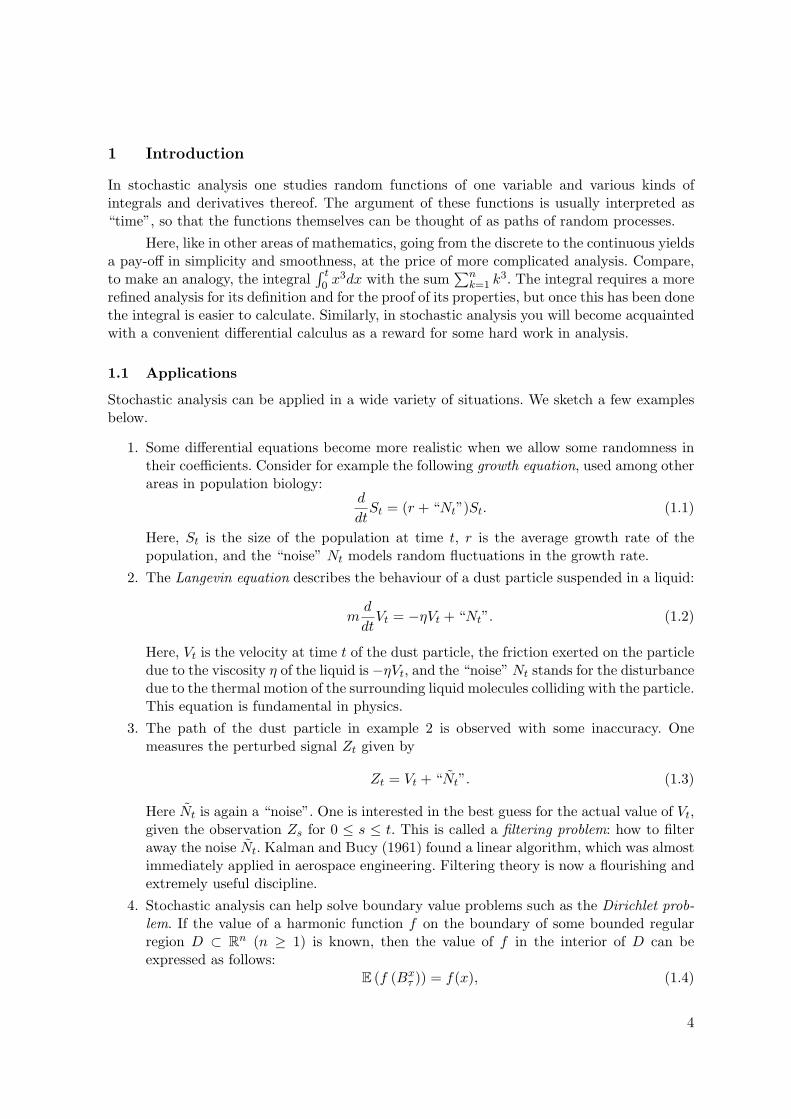
1. Some differential equations become more realistic when we allow some randomness intheir coefficients. Consider for example the following growth equation, used among otherareas in population biology:

d

dtSt = (r + “Nt”)St. (1.1)

Here, St is the size of the population at time t, r is the average growth rate of thepopulation, and the “noise” Nt models random fluctuations in the growth rate.

2. The Langevin equation describes the behaviour of a dust particle suspended in a liquid:

md

dtVt = −ηVt + “Nt”. (1.2)

Here, Vt is the velocity at time t of the dust particle, the friction exerted on the particledue to the viscosity η of the liquid is −ηVt, and the “noise” Nt stands for the disturbancedue to the thermal motion of the surrounding liquid molecules colliding with the particle.This equation is fundamental in physics.

3. The path of the dust particle in example 2 is observed with some inaccuracy. Onemeasures the perturbed signal Zt given by

Zt = Vt + “Nt”. (1.3)

Here Nt is again a “noise”. One is interested in the best guess for the actual value of Vt,given the observation Zs for 0 ≤ s ≤ t. This is called a filtering problem: how to filteraway the noise Nt. Kalman and Bucy (1961) found a linear algorithm, which was almostimmediately applied in aerospace engineering. Filtering theory is now a flourishing andextremely useful discipline.

4. Stochastic analysis can help solve boundary value problems such as the Dirichlet prob-lem. If the value of a harmonic function f on the boundary of some bounded regularregion D ⊂ Rn (n ≥ 1) is known, then the value of f in the interior of D can beexpressed as follows:

E (f (Bxτ )) = f(x), (1.4)

4

where “Bxt := x +

∫ t0 Nsds” is an “integrated noise” or Brownian motion, starting at

x, and τ denotes the time when this Brownian motion first reaches the boundary. (Aharmonic function f is a function satisfying ∆f = 0 with ∆ the Laplacian.)

5. Stochastic analysis has found extensive application nowadays in finance. A typical prob-lem is the following. At time t = 0 an investor buys stocks and bonds on the financialmarket, i.e., he divides his initial capital C0 into A0 shares of stock and B0 shares ofbonds. The bonds will yield a guaranteed interest rate r′, whereas the stock price St,measured relative to time 0, is assumed to satisfy the growth equation (1.1). With akeen eye on the market the investor sells stocks to buy bonds and vice versa. Suchdealings require no extra investments, and are called self-financing. Let At and Bt bethe amounts of stocks and bonds held at time t. The total value Ct of stocks and bondsat time t is

Ct = AtSt +Bter′t . (1.5)

The assumption that the tradings are self-financing can be expressed as:

dCt = AtdSt +Btd(er′t). (1.6)

An interesting question is now:

– What would our investor be prepared to pay at time 0 for a so-called Europeancall option, i.e., the right to buy at some later time T a share of stock at a prede-termined price K?

The rational answer, q say, was found by Black and Scholes (1973) through an analysisof the possible self-financing strategies leading from an initial investment q to the samepayoff as the option would do. Their formula is now being used on stock markets allover the world.

The goal of this course is to first make sense of the above equations, and then to work withthem.

1.2 What is noise?

In all the above examples the unexplained symbol Nt occurs, which is to be thought of as a“completely random” function of t, in other words, the continuous-time analogue of a sequenceof independent identically distributed random variables.

In a first attempt to catch this concept, it is tempting to try and meet the followingrequirements:

1. Nt is independent of Ns for t = s.2. The random variables Nt (t ≥ 0) all have the same probability distribution µ.3. E (Nt) = 0.

However, these requirements do not produce what we want. We shall show that such a “con-tinuous i.i.d. sequence” Nt is not measurable in t, unless it is identically zero.

Let µ denote the probability distribution of Nt, which by requirement 2 does not dependon t. If Nt is not a sure constant function of t, then there must be a value a ∈ R such thatp := P[Nt ≤ a] is neither 0 nor 1. Now consider the set E of time points where the noise is

5

less than a. It can be shown that with probability 1 the set E is not Lebesgue measurable.Without giving a full proof we can understand this as follows.

Let λ denote the Lebesgue measure on R. If E would be measurable, then by theindependence requirement 1 we would expect its relative share in any interval (c, d) to be p,by a continuous analogue of the law of large numbers:

λ (E ∩ (c, d)) = p (d− c) . (1.7)

On the other hand, it is known from measure theory that every measurable set B is arbitrarilythick somewhere with respect to λ, i.e., for every α < 1 an interval (c, d) can be found suchthat

λ (B ∩ (c, d)) > α(d− c) .

(cf. Halmos (1974) Theorem III.16.A: “Lebesgue’s density theorem”). So by (1.7), E is notmeasurable. This is a bad property of Nt because in view of (1.1), (1.2), (1.3) and (1.4), wewould like to be able to consider integrals of Nt.

For this reason, let us approach the problem from a different angle. Instead of Nt itself,let us consider directly the integral of Nt, and give it a name:

“Bt :=

∫ t

0Nsds”.

The three requirements on the evasive object Nt then translate into three quite sensiblerequirements for Bt.

BM1. For any 0 = t0 ≤ t1 ≤ . . . ≤ tn the random variables Btj+1 −Btj (j = 0, . . . , n− 1) areindependent.

BM2. Bt has stationary increments, i.e., the joint probability distribution of

(Bt1+s −Bu1+s, Bt2+s −Bu2+s, . . . , Btn+s −Bun+s)

does not depend on s ≥ 0, where ti > ui ≥ 0 for i = 1, 2, . . . , n are arbitrary.BM3. E (Bt) = 0 for all t ≥ 0.

We add a normalisation:

BM4. E(B21) = 1.

Still, these four requirements do not determine Bt. For example, the compensated Poissonjump process also satisfies them. Our fifth requirement fixes the process Bt uniquely (as willbecome clear later on):

BM5. t 7→ Bt is continuous a.s with probability 1.

The stochastic process Bt satisfying these requirements is called the Wiener process orBrownian motion. In the next chapter we shall give an explicit construction.

6

2 Brownian motion

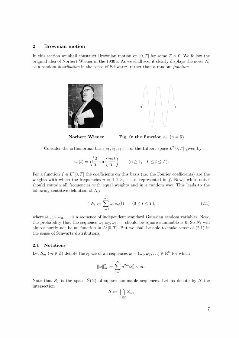
In this section we shall construct Brownian motion on [0, T ] for some T > 0. We follow theoriginal idea of Norbert Wiener in the 1930’s. As we shall see, it clearly displays the noise Nt

as a random distribution in the sense of Schwartz, rather than a random function.

0 T

Norbert Wiener Fig. 0: the function en (n = 5)

Consider the orthonormal basis e1, e2, e3, . . . of the Hilbert space L2[0, T ] given by

en (t) =

√2

Tsin

(nπt

T

)(n ≥ 1, 0 ≤ t ≤ T ).

For a function f ∈ L2[0, T ] the coefficients on this basis (i.e. the Fourier coefficients) are theweights with which the frequencies n = 1, 2, 3, . . . are represented in f . Now, ‘white noise’should contain all frequencies with equal weights and in a random way. This leads to thefollowing tentative definition of Nt:

“ Nt :=

∞∑n=1

ωnen(t) ” (0 ≤ t ≤ T ), (2.1)

where ω1, ω2, ω3, . . . is a sequence of independent standard Gaussian random variables. Now,the probability that the sequence ω1, ω2, ω3, . . . should be square summable is 0. So Nt willalmost surely not be an function in L2[0, T ]. But we shall be able to make sense of (2.1) inthe sense of Schwartz distributions.

2.1 Notations

Let Sm (m ∈ Z) denote the space of all sequences ω = (ω1, ω2, . . .) ∈ RN for which

∥ω∥2m :=∞∑n=1

n2mω2n <∞.

Note that S0 is the space l2(N) of square summable sequences. Let us denote by S theintersection

S :=∩m∈Z

Sm,

7

and by S ′ the union

S ′ :=∪m∈Z

Sm.

S consists of the rapidly decreasing sequences and S ′ of all the polynomially bounded ones.Under the pairing

⟨ω, x⟩ :=∞∑n=1

ωnxn,

the spaces Sm and S−m are each others dual, and S ′ is the dual of S. We have the followinginclusions:

S ′ ⊃ · · · ⊃ S−2 ⊃ S−1 ⊃ S0(= l2) ⊃ S1 ⊃ S2 ⊃ · · · ⊃ S.

Next let P denote the infinite product measure on RN that makes ω = (ω1, ω2, . . .) intoa sequence of independent standard Gaussian random variables. In a formula:

P(dω) :=∞⊗n=1

(1√2πe−

12ω2ndωn

).

The following lemma says that P-almost surely ωn increases slower than n, making the squareof their quotient summable.

Lemma 2.1 P(S−1) = P

ω ∈ Ω :

∞∑n=1

ω2n

n2<∞

= 1.

Proof. For n ∈ N, let Mn : RN → R denote the random variable

Mn(ω) :=

n∑j=1

ω2j

j2.

Since the ωj ’s are standard Gaussian, we have for all n ∈ N,

E(Mn) =

n∑j=1

1

j2≤ π2

6=: c

and therefore, for all k ∈ N and n ∈ N, by the Markov inequality,

P[Mn > k] ≤ 1

kE(Mn) ≤

c

k.

Since Mn(ω) is increasing in n for all ω, it follows that

P[Mn ≤ k for all n] = P(∩n∈N

[Mn ≤ k])= lim

n→∞P[Mn ≤ k] ≥ 1− c

k,

and henceP(S−1) = P

(∪k∈N

∩n∈N

[Mn ≤ k])= lim

k→∞

(1− c

k

)= 1.

8

2

Since S−1 ⊂ S ′, ω also lies in S ′ with probability 1. Now, S ′ consists of the sequencesof Fourier coefficients of the tempered distributions, and the latter are a good class to workwith. So we shall henceforth use S ′ as our sample space Ω. The connection with the space ofdistributions is as follows.

Let D[0, T ] denote the space of infinitely differentiable functions on [0, T ] with compactsupport inside (0, T ). A function f ∈ D[0, T ] determines a sequence of real numbers

νn := ⟨en, f⟩ :=∫ T

0en(t)f(t)dt (n ∈ N).

For all even m ∈ N, the property that f is m times continuously differentiable implies thatν ∈ Sm by partial integration:∫ T

0|f (m)(t)|2dt =

∞∑n=1

⟨en, f (m)⟩2 =∞∑n=1

⟨e(m)n , f⟩2

=

∞∑n=1

(nπT

)2m⟨en, f⟩2 =

(πT

)2m∥ν∥2m.

Conversely, ν ∈ Sm implies that f (m) ∈ L2[0, t], so f ism−1 times continuously differentiable.Now, a sequence ν1, ν2, . . . is said to converge to an element ν of S (ν is itself a sequence ofnumbers!) if it converges in Sm for everym. On the other hand, a sequence f1, f2, . . . in D[0, T ]

is said to converge to an f ∈ D[0, T ] if for all m ∈ N the sequence f(m)1 , f

(m)2 , . . . converges

uniformly to f (m). Therefore the topology on S is carried over to D[0, T ].

2.2 Definition of Brownian motion

We now define white noise N on [0, T ] by

N : Ω×D[0, T ] : (ω, f) 7→∞∑n=1

ωn⟨en, f⟩.

For fixed ω ∈ Ω, the map N(ω) : f 7→ N(ω, f) is a distribution on [0, T ]. Hence, with themeasure P being defined on Ω, our map N becomes a random distribution. On the otherhand, for fixed f ∈ D[0, T ] the map

Nf : ω 7→ N(ω, f)

is a Gaussian random variable with mean zero and variance ∥f∥2:

E(Nf ) = E( ∞∑i=1

ωi⟨ei, f⟩)= 0

E(N2f ) = E

( ∞∑i=1

∞∑j=1

ωiωj⟨ei, f⟩⟨ej , f⟩)=

∞∑i=1

⟨ei, f⟩2 = ∥f∥2.

9

It follows that the map f 7→ Nf can be extended to a Hilbert space isometry L2[0, T ] →L2(Ω,P). Indeed, if fi is a sequence of functions in D[0, T ] such that ∥fi − f∥ → 0 (i → ∞)for some f ∈ L2[0, T ], then the sequence (Nf )

∞i=1 is a Cauchy-sequence in L2(Ω,P):

∥Nfi − Nfj∥2 = E((Nfi − Nfj )

2) = E(N2fi−fj

) = ∥fi − fj∥2.

So it has a limit, Nf say. Moreover, the map f 7→ Nf is isometric:

E(N2f ) = ∥f∥2 ∀f ∈ L2[0, T ]. (2.2)

Hence again for all f, g ∈ L2[0, T ]:

E(Nf ) = 0 , E(NfNg) = ⟨f, g⟩ . (2.3)

However, the extension from N on Ω×D[0, T ] to N on Ω×L2[0, T ] has a price: whereasNf (f ∈ D[0, T ]) is a random element of (D[0, T ])′, Nf (f ∈ L2[0, T ]) is not a random elementof (L2[0, T ])′ = L2[0, T ], the reason being that Nf (ω) is only defined for fixed f ∈ L2[0, T ]and almost all ω ∈ Ω. The set of those ω for which Nf (ω) is defined for all f ∈ L2[0, T ] hasmeasure 0.

We employ the extension from N to N in order to define Brownian motion:

Definition. Brownian motion over the time interval [0, T ] is the family (Bt)t∈[0,T ] of randomvariables Ω → R given by

Bt(ω) := N1[0,t](ω).

We finally show that this definition meets all our requirements.

Proposition 2.2 Bt satisfies the conditions BM1–BM4 of Section 1. Moreover:

BM5. There exists a version of (Bt)t∈[0,T ] such that t 7→ Bt is continuous.BM6. With probability 1, t 7→ Bt has infinite variation over every time interval and is

therefore nowhere differentiable.

Proof. From the construction of N it is clear that for any f1, f2, . . . , fk ∈ L2[0, T ] therandom variables Nf1 , Nf2 , . . . , Nfk are jointly Gaussian. A standard result in probabilitytheory ensures that

i. jointly Gaussian random variables are independent as soon as they are uncorrelated,ii. their joint probability distribution depends only on their expectations and their corre-

lations.

So the independence of the increments of Brownian motion (BM1) follows from theorthogonality of the functions 1[tj ,tj+1) = 1[0,tj+1) − 1[0,tj) (j = 0, . . . , n − 1), since N mapsorthogonal functions f and g to uncorrelated random variables (by (2.3)). The stationarityof the increments (BM2) follows from the fact that the inner products of the functions1[uj+s,tj+s) (j = 1, . . . , n) do not depend on s. Properties BM3 and BM4 are obvious:

E(Bt) = E(N1[0,t]) = 0, E(B2t ) = ∥1[0,t]∥2 = t. The proof of properties BM5 and BM6

requires some preparation and is deferred to Sections 2.3–2.4. 2

From (2.3) it follows that for all s, t ≥ 0:

E(BsBt) = ⟨1[0,s], 1[0,t]⟩ = s ∧ t . (2.4)

10

2.3 Continuity of paths and the problem of versions

The continuity of paths t 7→ Bt(ω) with ω ∈ Ω is a somewhat subtle matter.

First, let us make clear that the continuity of the curve t 7→ Bt in L2(Ω,P) is not at all

sufficient to ensure continuity of the paths t 7→ Bt(ω).

Example 2.1.¡ Let Ω = [0, 1] with Lebesgue measure P. Let Xt (t ∈ [0, 1]) denote the process

Xt(ω) := 1[0,t](ω) =

0 if t ≤ ω,

1 if t > ω.

So Xt(ω), far from being continuous, moves by making a single jump at a random time.However, t 7→ Xt is a continuous curve in L2(Ω,P), since

∥Xt −Xs∥2 =∫ t

sdu = t− s (s ≤ t) .

Second, let us observe that a description of a curve in L2(Ω,P), such as t 7→ Bt, cannever be sufficient to ensure pathwise continuity. This is shown by the following example.

Example 2.2.¡ Take (Ω,P) as in the previous example. Now let Yt(ω) be given by

Yt(ω) =

1 if ω − t is irrational

0 if ω − t is rational.

Let Zt(ω) = 1 for all ω ∈ Ω, t ∈ [0, 1]. Clearly, t 7→ Zt(ω) is constant, hence continuous forall ω ∈ Ω, whereas t 7→ Yt(ω) is discontinuous for all ω ∈ Ω. Nevertheless, for any fixed valueof t, Yt and Zt are almost surely equal, so they correspond to the same curve in L2(Ω,P).

These observations leads us to the following definition:

Definition. We say that a process Yt ∈ L2(Ω,P) (t ∈ [0, T ]) is a version of a processZt ∈ L2(Ω,P) (t ∈ [0, T ]) if

∀t ∈ [0, T ] : Yt(ω) = Zt(ω) for almost all ω ∈ Ω.

This said, we proceed to prove that Brownian Motion has a version with continuouspaths, as claimed in property BM5 in Proposition 2.2.

Proof. For the fourth moment of a centered Gaussian random variable ξ we have E(ξ4) =3Var(ξ)2. Hence for the process Bt we have

E(|Bt −Bs|4

)= 3|t− s|2.

Now fix α ∈ (0, 1/4) and put ε := 1 − 4α > 0. Then, for all s, t ∈ [0, T ], we have by theMarkov inequality,

P[|Bt −Bs| ≥ |t− s|α

]≤ |t− s|−4αE

(|Bt −Bs|4

)≤ 3|t− s|2−4α

= 3|t− s|1+ε,

11

so that for all n ∈ N and 0 ≤ k < 2n,

P[|B(k+1)2−nT −Bk2−nT | ≥ 2−nα

]≤ 3× 2−n(1+ε),

and hence

∞∑n=1

2n−1∑k=0

P[|B(k+1)2−nT −Bk2−nT | ≥ 2−nα

]≤

∞∑n=1

2n−1∑k=0

3× 2−n2−nε = 3

∞∑n=1

2−nε =3

2ε − 1<∞.

By the first Borel-Cantelli lemma it follows that if An denotes the event

An :=[∃0 ≤ k < 2n : |B(k+1)2−nT −Bk2−nT | ≥ 2−nα

],

then with probability 1 only finitely many An’s happen. So for almost all ω ∈ Ω there existsM(ω) ∈ N such that An does not occur for n ≥M(ω), i.e., for all n ≥M(ω) we have

∀0 ≤ k < 2n : |B(k+1)2−nT (ω)−Bk2−nT (ω)| < 2−nα. (2.5)

Now fix an ω for which the latter holds, and let s and t be two points in the set Q ofdyadic rationals of T,

Q :=k2−nT

∣∣∣ n, k ∈ N, 0 ≤ k ≤ 2n,

such that |s − t| ≤ 2−M(ω)T . Choose n ≥ M(ω) such that 2−(n+1)T ≤ |s − t| < 2−nT . Letk ∈ N be such that k2−nT has distance less than 2−nT to both s and t. We may then writethe dyadic representation

s = k2−nT +l∑

i=1

σi2−(n+i)T

t = k2−nT +m∑j=1

τi2−(n+j)T,

where l,m ∈ N and σi, τj ∈ −1, 0, 1 for i = 1, . . . , l and j = 1, . . . ,m. By (2.5) we may nowconclude that

|Bt(ω)−Bs(ω)| <l∑

i=1

|σi2−(n+i)α|+m∑j=1

|τj2−(n+j)α|

≤ 2

1− 2−α2−(n+1)α

≤ 2

Tα(1− 2−α)|s− t|α.

It follows that the restriction of the function t 7→ Bt(ω) to Q may be extended to a continuousfunction t 7→ Bt(ω) on all of [0, T ].

12

It remains to show that Bt is a version of Bt. Choose t ∈ [0, T ] and let t1, t2, . . . be asequence in Q tending to t. Let φ : R → R be a bounded, continuous and strictly increasingfunction. Then∫

Ω|φ(Bt(ω))− φ(Bt(ω))|2P(dω) = ∥φ(Bt)− φ(Bt)∥2 = lim

i→∞∥φ(Bti)− φ(Bti)∥2 = 0,

since t 7→ Bt is continuous in L2(Ω,P) and t 7→ Bt is pointwise continuous, and therefore also

continuous in L2(Ω,P) by bounded convergence. 2

Henceforth, when speaking of Bt we shall always mean its continuous version and dropthe tilde from the notation.

2.4 Roughness of paths

Although the path of Brownian motion is continuous, it is extremely rough. This is expressedby the following basic lemma, which we shall need to prove property BM6 in Proposition2.2.

Lemma 2.3 Let 0 = t(n)0 < t

(n)1 < · · · < t

(n)n = T be a family of partitions of the interval

[0, T ] that gets arbitrarily fine for n→ ∞, in the sense that

limn→∞

max0≤j<n

|t(n)j+1 − t(n)j | = 0.

Then

L2 − limn→∞

n−1∑j=0

(Bt(n)j+1

−Bt(n)j

)2 = T.

Proof. Abbreviate ∆Bj = Bt(n)j+1

−Bt(n)j

and ∆tj = t(n)j+1 − t

(n)j . Let δn = maxj ∆tj . Then

∥∥∥∑j

(∆Bj)2 − T

∥∥∥2 = E[(∑

j

(∆Bj)2 − T

)2]= E

(∑i,j

(∆Bi)2(∆Bj)

2)− 2TE

(∑j

(∆Bj)2)+ T 2

=∑j

E((∆Bj)4) +

∑i =j

E((∆Bi)2)E((∆Bj)

2)− 2T(∑

j

∆tj

)+ T 2

=∑j

3(∆tj)2 +

∑i=j

(∆ti)(∆tj)− T 2

= 2∑j

(∆tj)2

≤ 2δn∑j

∆tj

= 2δnT,

13

where again we have used the fact that the fourth moment of a centered Gaussian randomvariable ξ is given by E

(ξ4)= 3Var(ξ)2. As limn→∞ δn = 0, the statement follows. 2

We may write the message of Lemma 2.3 symbolically as

“(dBt)2 = dt”, (2.6)

saying that “Brownian motion has quadratic variation growing linearly with time”. Thisexpression will acquire a precise meaning during the sequel of this course. For the moment,let us just say that Bt has large fluctuations on a small scale, namely

dBt is of order√dt(≫ dt

).

To prove BM6 of Proposition 2.2 we need one more preparatory lemma, which appliesto a general sequence of random variables.

Lemma 2.4 Let X1, X2, X3, . . . be a sequence of real-valued random variables such that forsome p > 0,

limn→∞

E (|Xn|p) = 0 for some p > 0.

Then there exists a subsequence (Xnk)∞k=1 tending to 0 almost surely.

Proof. Choose a subsequence such that∑∞

k=1 E(|Xnk|p) < ∞. By Chebyshev’s inequality

we have, for all m ∈ N,

P[|Xnk

| ≥ 1

m

]≤ mpE (|Xnk

|p) ,

and therefore, for all m ∈ N, ∑k

P[|Xnk

| ≥ 1

m

]<∞.

The first Borel-Cantelli lemma now implies that for any m,

P[|Xnk

| ≥ 1

mfor finitely many k

]= 1.

By σ-additivity the intersection over m of the event between brackets also has probability 1:

P[∀m ∈ N ∃K ∈ N∀k ≥ K : |Xnk

| < 1

m

]= 1,

i.e., Xnk→ 0 almost surely as k → ∞. 2

We are finally ready to finish our proof of Proposition 2.2:

Proof. By Lemmas 2.3 and 2.4 (with p = 2) there exists an increasing sequence (nk) suchthat, for almost all ω ∈ Ω,

limk→∞

n−1∑j=0

(B

t(nk)

j+1

(ω)−Bt(nk)

j

(ω))2

= T.

14

Fix an ω ∈ Ω for which this holds. Let

εnk:= max

j|∆Bj | := max

0≤j<nk

∣∣∣∣Bt(nk)

j+1

(ω)−Bt(nk)

j

(ω)

∣∣∣∣ .Then limk→∞ εnk

= 0 by the uniform continuity of t 7→ Bt (which is a continuous function onthe compact interval [0, T ]). It follows that,

nk−1∑j=0

|∆Bj | ≥nk−1∑j=0

1

εnk

|∆Bj |2 ∼1

εnk

T −→ ∞ as k → ∞

2

This concludes the construction of Brownian motion. In the next sections we shall seethat Brownian motion is the building block of stochastic analysis.

The construction of Brownian motion induces a probability measure on the set of allcontinuous functions [0, T ] → R, which is called the Wiener measure.

It can be proved that all random variables in L2(Ω,P) can be represented in a natu-ral way as integrals of products of increments of Brownian motion. This is Wiener’s chaosexpansion, (Wiener (1938).)

15

3 Stochastic integration: the Gaussian case

This section serves as a motivation for the Ito-calculus presented in Sections 4 and 5.

3.1 The stochastic integral of a non-random function

If fn ∈ L2[0, T ] is a step function, i.e.,

fn(t) =

n−1∑j=0

c(n)j 1[tj ,tj+1)(t) (0 = t0 < t1 < · · · < tn = T ),

then from the definition Bt := N1[0,T ]it follows that

Nfn =

n−1∑j=0

c(n)j (Btj+1 −Btj ),

which is precisely what we would mean by the integral∫ T0 fn(t)dBt. Moreover, if fn → f in

L2[0, T ], then Nfn → Nf in L2(Ω,P) by the isometric property of N described in Section 2.2.So f 7→ Nf maps L2[0, T ] into the Gaussian random variables on (Ω,P). It is therfore naturalto define for all f ∈ L2[0, T ]: ∫ T

0f(t)dBt(ω) := Nf (ω).

3.2 The Ornstein-Uhlenbeck process

In 1908 Langevin proposed an equation in order to describe the motion of a particle suspendedin a liquid. He wanted to give a treatment which was more refined and more in harmony withNewtonian mechanics than the above Brownian motion model. Let Vt denote the velocity ofthe particle at time t. According to Newton’s second law the derivative d

dtVt should be equalto the sum of the forces acting on the particle (see example 2 in Section 1: we take the massof the particle equal to 1). Langevin wrote

d

dtVt = −ηVt + σNt,

where the first term on the r.h.s. models the friction due to the viscosity η of the liquid andthe second term describes the sum total of the erratic collisions of liquid molecules againstthe particle, σ being the strength of the noise.

In the spirit of the preceding discussion we rewrite the Langevin equation as

dVt = −ηVtdt+ σdBt, (3.1)

which again is shorthand for the integral equation

Vt − Vs = −η∫ t

sVudu+ σ(Bt −Bs) (3.2)

in L2(Ω,P). This equation was solved by Ornstein and Uhlenbeck (1930) in the following way.Rewrite (3.1) as

d(eηtVt) = σeηtdBt.

16

t T

1

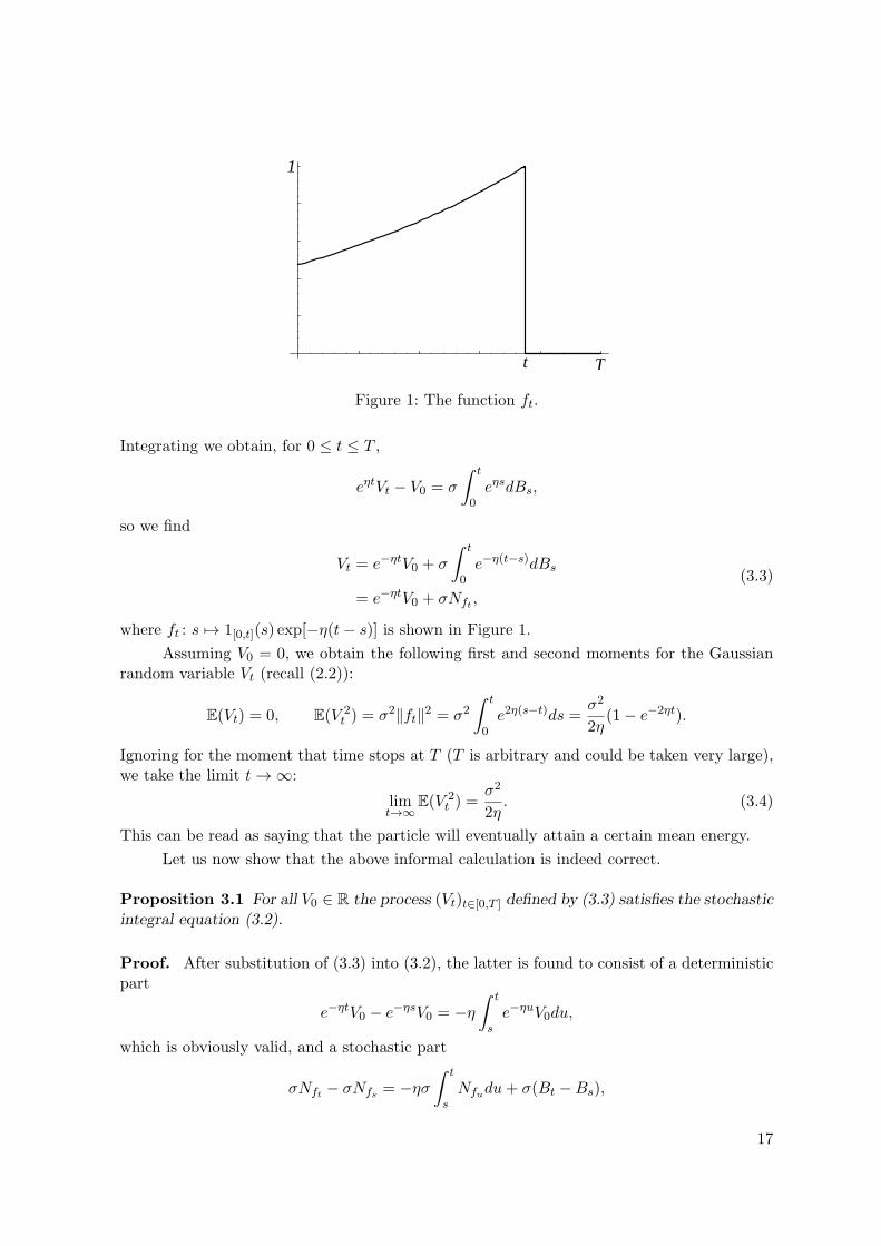
Figure 1: The function ft.

Integrating we obtain, for 0 ≤ t ≤ T ,

eηtVt − V0 = σ

∫ t

0eηsdBs,

so we find

Vt = e−ηtV0 + σ

∫ t

0e−η(t−s)dBs

= e−ηtV0 + σNft ,

(3.3)

where ft : s 7→ 1[0,t](s) exp[−η(t− s)] is shown in Figure 1.

Assuming V0 = 0, we obtain the following first and second moments for the Gaussianrandom variable Vt (recall (2.2)):

E(Vt) = 0, E(V 2t ) = σ2∥ft∥2 = σ2

∫ t

0e2η(s−t)ds =

σ2

2η(1− e−2ηt).

Ignoring for the moment that time stops at T (T is arbitrary and could be taken very large),we take the limit t→ ∞:

limt→∞

E(V 2t ) =

σ2

2η. (3.4)

This can be read as saying that the particle will eventually attain a certain mean energy.

Let us now show that the above informal calculation is indeed correct.

Proposition 3.1 For all V0 ∈ R the process (Vt)t∈[0,T ] defined by (3.3) satisfies the stochasticintegral equation (3.2).

Proof. After substitution of (3.3) into (3.2), the latter is found to consist of a deterministicpart

e−ηtV0 − e−ηsV0 = −η∫ t

se−ηuV0du,

which is obviously valid, and a stochastic part

σNft − σNfs = −ησ∫ t

sNfudu+ σ(Bt −Bs),

17

which can be obtained by applying the map N to both sides of the following identity inL2[0, T ]:

ft − fs = −η∫ t

sfudu+ 1[s,t] (0 ≤ s ≤ t ≤ T ).

The proof of this identity is left as an exercise. 2

3.3 Some hocus pocus

Let us again consider the Ornstein-Uhlenbeck process (Vt)t∈[0,T ] and perform some suggestiveformal manipulations.

It is tempting to write

d(V 2t ) = 2VtdVt = 2Vt(−ηVtdt+ σdBt),

which, under the formal assumption that Vt and dBt are independent quantities, leads to

dE(V 2t ) = −2ηE(V 2

t )dt+ 2σE(Vt)E(dBt)

= −2ηE(V 2t )dt.

However, this result is false since it would imply that E(V 2t ) tends to 0 as t→ ∞, contradicting

(3.4).

What went wrong? How should we change the rules of formal manipulation of differen-tials? Should we reject the independence assumption Vt ⊥⊥ dBt? This is indeed a possibility,and leads to the so-called “stochastic calculus of Stratonovic”. However, we shall not reject thisindependence assumption, but instead follow Ito and reconsider the first step d(V 2

t ) = 2VtdVt.

Let us take seriously the formula (dBt)2 = dt in (2.6), implying that (dVt)

2 = σ2dt, andlet us expand d(V 2

t ) to second order in dVt:

d(V 2t ) = 2VtdVt + (dVt)

2

= (Vt + dVt)2 − V 2

t

= 2Vt(−ηVtdt+ σdBt) + σ2dt.

This gives, upon calculation of expectations,

dE(V 2t ) = −2ηE(V 2

t )dt+ σ2dt,

leading indeed to the correct equilibrium value (3.4). Note the occurrence of the extra termσ2dt compared to the previous calculation. This term is the essential ingredient to make endsmeet.

The above argument is heuristic at this stage, because both Bt and Vt are functions ofinfinite variance, and hence nowhere differentiable. Still, we shall see that it makes perfectsense in the right interpretation. This will be clarified in Sections 4 and 5.

18

4 The Ito-integral

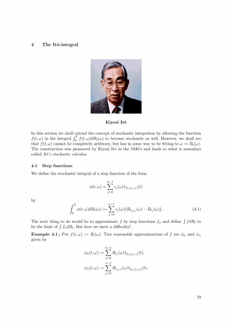
Kiyosi Ito

In this section we shall extend the concept of stochastic integration by allowing the functionf(t, ω) in the integral

∫ T0 f(t, ω)dBt(ω) to become stochastic as well. However, we shall see

that f(t, ω) cannot be completely arbitrary, but has in some way to be fitting to ω 7→ Bt(ω).The construction was pioneered by Kiyosi Ito in the 1940’s and leads to what is nowadayscalled Ito’s stochastic calculus.

4.1 Step functions

We define the stochastic integral of a step function of the form

ϕ(t, ω) =

n−1∑j=0

cj(ω)1[tj ,tj+1)(t)

by ∫ T

0ϕ(t, ω)dBt(ω) :=

n−1∑j=0

cj(ω)(Btj+1(ω)−Btj (ω)

). (4.1)

The next thing to do would be to approximate f by step functions fn and define∫fdBt to

be the limit of∫fndBt. But here we meet a difficulty!

Example 4.1.¡ Put f(t, ω) := Bt(ω). Two reasonable approximations of f are ϕn and ψn

given by

ϕn(t, ω) :=

n−1∑j=0

Btj (ω)1[tj ,tj+1)(t),

ψn(t, ω) :=

n−1∑j=0

Btj+1(ω)1[tj ,tj+1)(t),

19

where t0, t1, . . . , tn are defined as in Lemma 2.3 in Section 2.4 (and are not ω-dependent).However, from our definition (4.1) we find that∫ T

0ψndBt −

∫ T

0ϕndBt =

n−1∑j=0

(∆Bj)2,

which, according to Lemma 2.3, does not tend to 0 as n→ ∞ but to the constant T . In otherwords, the variation of the path t 7→ Bt is too large for

∫BtdBt to be defined in a casual way.

We now introduce a requirement on our function f for the approximation by stepfunctions fn to work nicely.

Definition. Let Ft denote the σ-field generated by Bs | 0 ≤ s ≤ t . Let F := FT . Astochastic process on the probability space (Ω,F ,P) of Brownian motion is a measurablemap [0, T ]× Ω → R. The process will be called adapted to the family of σ-fields (Ft)t∈[0,T ] ifω 7→ f(t, ω) is Ft-measurable for all t ∈ [0, T ].

The space L2(Ω,Ft,P) of square-integrable Ft-measurable functions may be thought ofas those functions of ω ∈ Ω that are fully determined by the initial segment [0, t] → R : s 7→Bs(ω) of the Brownian motion. In other words, g ∈ L2(Ω,Ft,P) when g(ω) = g(ω′) as soonas Bs(ω) = Bs(ω

′) for all s ∈ [0, t].

Let L2(B, [0, T ]) denote the space of all adapted stochastic processes f : [0, T ]×Ω → Rthat are square integrable:

∥f∥2L2(Ω,P) =

∫ T

0dt

∫Ωf(t, ω)2P(dω) <∞.

The natural inner product that makes L2(B, [0, T ]) into a real Hilbert space is

⟨f, g⟩ :=∫ T

0dt

∫Ωf(t, ω)g(t, ω)P(dω)

= E(∫ T

0f(t, ·)g(t, ·)dt

).

We note that the step functions ϕn in the last example are adapted, since ϕn(t, ω)= Btj

for t ∈ [tj , tj+1), so that ϕn(t, ω) only depends on past values of B. On the other hand, ψn isnot adapted, since at time t ∈ [tj , tj+1) it already anticipates the Brownian motion at timetj+1: ψn(t, ω)= Btj+1(ω).

The next theorem is a crucial property of stochastic integrals of adapted step functions.

Proposition 4.1 (The Ito-isometry) Let ϕ be a step function in L2(B, [0, T ]), and let

I0(ϕ)(ω) :=∫ T

0ϕ(t, ω)dBt(ω)

be its stochastic integral according to (4.1). Then I0 is an isometry:

∥I0(ϕ)∥L2(Ω,P) = ∥ϕ∥L2(B), (4.2)

20

i.e., ∫ΩP(dω)

(∫ T

0ϕ(t, ω)dBt(ω)

)2

=

∫ T

0dt

∫ΩP(dω)ϕ2(t, ω).

Proof. By adaptedness, ci in (4.1) is independent of ∆Bj := Btj+1 − Btj for 0 ≤ i ≤ j.Therefore

∥I0(ϕ)∥2L2(Ω,P) = E((n−1∑

j=0

cj∆Bj

)2)

=n−1∑i=0

n−1∑j=0

E(cicj∆Bi∆Bj

)=

n−1∑j=0

E(c2j (∆Bj)

2)+ 2

∑i<j

E(cicj∆Bi

)E(∆Bj

)=

n−1∑j=0

E(c2j )E((∆Bj)

2)

=n−1∑j=0

E(c2j )∆tj ,

where we use that E(∆Bj) = 0, E((∆Bj)2) = ∆tj (recall BM3-BM4 in Section 1). On the

other hand,

∥ϕ∥2L(B,[0,T ]) =

∫ T

0E([ n−1∑

j=0

cj1[tj ,tj+1)(t)]2)

dt

=

n−1∑i=0

n−1∑j=0

(∫ T

01[ti,ti+1)(t)1[tj ,tj+1)(t)dt

)E(cicj)

=

n−1∑j=0

∆tjE(c2j ).

The two expressions are the same. 2

4.2 Arbitrary functions

To go from step functions to arbitrary functions we need the following.

Lemma 4.2 Every function f ∈ L2(B, [0, T ]) can be approximated arbitrarily well by stepfunctions in L2(B, [0, T ]).

Proof of Lemma 4.2. We divide the proof into three steps of successive approximation.

Step 1. Every bounded pathwise continuous g ∈ L2(B, [0, T ]) can be approximated by asequence of step functions.

21

Proof. Partition the interval [0, T ] into n pieces by times (tj)nj=1 in the customary

way. Define

ϕn(t, ω) :=

n−1∑j=0

g(tj , ω)1[tj ,tj+1)(t).

Then, since t 7→ g(t, ω) is continuous and maxj |∆tj | → 0 for all ω ∈ Ω, we have

limn→∞

∫ T

0

(g(t, ω)− ϕn(t, ω)

)2dt = 0.

Hence, by bounded convergence,

limn→∞

E(∫ T

0

(g(t, ω)− ϕn(t, ω)

)2dt

)= 0.

2

Step 2. Every bounded h ∈ L2(B) can be approximated by a sequence of bounded continuousfunctions in L2(B).

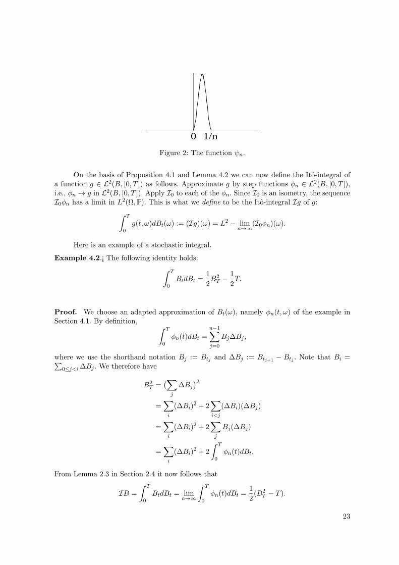
Proof. Suppose |h| ≤ M . For n ∈ N, let ψn be a non-negative continuous functionof the form given in Figure 2, with the properties ψn(x) = 0 for x /∈ [0, 1/n] and∫∞−∞ ψn(x)dx = 1. Define

gn(t, ω) :=

∫ t

0ψn(t− s)h(s, ω)ds.

(Think of ψn as a “mollifier” of h.) Then t 7→ gn(t, ω) is continuous for all ω, and|gn| ≤M . Moreover, for all ω,

limn→∞

∫ T

0

(gn(s, ω)− h(s, ω)

)2ds = 0,

since ψn constitutes an approximate identity. Again, by bounded convergence,

limn→∞

E(∫ T

0

(gn(s, ω)− h(s, ω)

)2ds)= 0.

2

Step 3. Every f ∈ L2(B, [0, T ]) can be approximated by bounded functions in L2(B, [0, T ]).(This is in fact a general property L2-spaces.)

Proof. Let f ∈ L2(B) and put hn(t, ω) := (−n) ∨ (n ∧ f(t, ω)). Then

∥f − hn∥2L2(B) ≤∫ T

0dt

∫ΩP(dω) 1[n,∞)(|f(t, ω)|)f(t, ω)2,

which tends to 0 as n→ ∞ by dominated convergence. 2

22

0 1/n

Figure 2: The function ψn.

On the basis of Proposition 4.1 and Lemma 4.2 we can now define the Ito-integral ofa function g ∈ L2(B, [0, T ]) as follows. Approximate g by step functions ϕn ∈ L2(B, [0, T ]),i.e., ϕn → g in L2(B, [0, T ]). Apply I0 to each of the ϕn. Since I0 is an isometry, the sequenceI0ϕn has a limit in L2(Ω,P). This is what we define to be the Ito-integral Ig of g:∫ T

0g(t, ω)dBt(ω) := (Ig)(ω) = L2 − lim

n→∞(I0ϕn)(ω).

Here is an example of a stochastic integral.

Example 4.2.¡ The following identity holds:∫ T

0BtdBt =

1

2B2

T − 1

2T.

Proof. We choose an adapted approximation of Bt(ω), namely ϕn(t, ω) of the example inSection 4.1. By definition, ∫ T

0ϕn(t)dBt =

n−1∑j=0

Bj∆Bj ,

where we use the shorthand notation Bj := Btj and ∆Bj := Btj+1 − Btj . Note that Bi =∑0≤j<i∆Bj . We therefore have

B2T =

(∑j

∆Bj

)2=∑i

(∆Bi)2 + 2

∑i<j

(∆Bi)(∆Bj)

=∑i

(∆Bi)2 + 2

∑j

Bj(∆Bj)

=∑i

(∆Bi)2 + 2

∫ T

0ϕn(t)dBt.

From Lemma 2.3 in Section 2.4 it now follows that

IB =

∫ T

0BtdBt = lim

n→∞

∫ T

0ϕn(t)dBt =

1

2(B2

T − T ).

23

2

Note that the integral in the above example is actually different from what it would befor a smooth function f with f(0) = 0, namely:

∫ T0 f(t)df(t) = 1

2f(T )2. What the example

shows is that “stochastic integration is ordinary integration except that the diagonal termsmust be left out”. This will be made precise in Section 5, where we shall encounter a fasterway to calculate stochastic integrals.

4.3 Martingales

In Section 4.4 we shall prove that the Ito-integral w.r.t. Brownian motion of an adaptedsquare-integrable stochastic process always has a continuous version. For this we shall need theinterlude on martingales described in this section. For a general introduction on martingaleswe refer to the book by D. Williams (1991).

Definition. By the conditional expectation at time t ∈ [0, T ] of a random variable X ∈L2(Ω,P) we shall mean its orthogonal projection onto L2(Ω,Ft,P), the space of randomvariables that are determined by the Brownian motion up to time t. We denote this projectionby E(X | Ft), or briefly Et(X).

In words, Et(X)(ω) is the best estimate (in the sense of least mean square error) that can bemade of X(ω) on the basis of the knowledge of Bs(ω) for 0 ≤ s ≤ t.

Definition. An adapted process M ∈ L2(B, [0, T ]) is called a martingale (w.r.t. Brownianmotion) if

Es(Mt) =Ms for 0 ≤ s ≤ t ≤ T .

A martingale is a “fair game”: the expected value at any time in the future is equal to thecurrent value. Note that Brownian motion itself is a martingale, since for 0 ≤ s ≤ t ≤ T ,

Es(Bt) = Es(Bs + (Bt −Bs)) = Bs + Es(Bt −Bs) = Bs,

because Bt − Bs is independent of and hence orthogonal to any function in L2(Ω,Fs,P), inparticular, to Brownian motion.

Theorem 4.3 The stochastic integral of an adapted step function is a martingale with con-tinuous paths.

Proof. This follows directly from the fact that Brownian motion has continuous paths andsatisfies the martingale property (use the definition of the stochastic integral of a step functiongiven in (4.1) in Section 4.1). 2

The following powerful tool will help us prove that the Ito-integral of any process inL2(B, [0, T ]) possesses a continuous version.

Theorem 4.4 (The Doob martingale inequality) IfMt is a martingale with continuouspaths, then for all p ≥ 1 and λ > 0,

P[ sup0≤t≤T

|Mt| ≥ λ] ≤ 1

λpE(|MT |p).

24

Proof. We may assume that E(|MT |p) < ∞, otherwise the statement is trivially true. LetZt := |Mt|p. Then, since x 7→ |x|p is a convex function, Jensen’s inequality gives that Zt issub-martingale: for all 0 ≤ s ≤ t ≤ T ,

Es(Zt) = Es(|Mt|p) ≥ |Es(Mt)|p = |Ms|p = Zs.

It follows in particular that E(|Ms|p) < ∞ for all s ∈ [0, T ]. Let us discretise time and firstprove a discrete version of the Doob inequality. To that end we fix n ∈ N and put tk = kT/n,k = 0, 1, . . . , n. Let K(ω) denote the smallest value of k for which Ztk ≥ λp, if this occurs atall. Otherwise, put K(ω) = ∞. Then we may write, since [K = k] ∈ Ftk ,

P[ max0≤k≤n

|Mtk | ≥ λ] =

n∑k=0

P[K = k]

≤n∑

k=0

1

λpE(1[K=k]Ztk)

≤n∑

k=0

1

λpE(1[K=k]E(ZT |Ftk)

)=

n∑k=0

1

λpE(1[K=k]ZT )

≤ 1

λpE(ZT )

=1

λpE(|MT |p).

Here, the second inequality uses the sub-martingale property at time tk. To get the same forcontinuous time, let An denote the event [max0≤k≤n |Mtk | ≥ λ]. Then we have A1 ⊂ A2 ⊂A4 ⊂ A8 ⊂ · · · , and so, t 7→Mt being continuous,

P[ sup0≤t≤T

|Mt| ≥ λ] = P( ∞∪n=0

A2n)= lim

n→∞P(A2n) ≤

1

λpE(|MT |p).

2

4.4 Continuity of paths

We shall use the martingale inequality of Theorem 4.4 in Section 4.3 to prove the existence ofa continuous version for our stochastic integrals. Two stochastic processes It and Jt are calledversions of each other if It(ω) and Jt(ω) are equal for all t ∈ [0, T ] and almost all ω ∈ Ω.(recall Definition 2.3 in Section 2.3).

Theorem 4.5 Let f ∈ L2(B, [0, T ]). Let

It(ω) =

∫ t

0f(s, ω)dBs(ω).

Then there exists a version Jt of It such that t 7→ Jt(ω) is continuous for almost all ω ∈ Ω.

25

Proof. The point of the proof is to turn continuity in L2(Ω,P) into continuity of paths. Thisrequires several estimates.

Let ϕn ∈ L2(B, [0, T ]) be an approximation of f by step functions. Put

In(t, ω) =

∫ t

0ϕn(s, ω)dBs(ω).

By Lemma 4.3 in Section 4.3, In is a pathwise continuous martingale for all n. The sameholds for the differences In− Im. Therefore, by Doob’s martingale inequality (with p = 2 andλ = ε) and the Ito-isometry, we have

P

[sup

0≤t≤T|In(t)− Im(t)| ≥ ε

]≤ 1

ε2E((In(T )− Im(T ))2

)=

1

ε2

∫ T

0E((ϕn(t)− ϕm(t))2

)dt

=1

ε2∥ϕn − ϕm∥2L2(B,[0,T ]),

which tends to 0 as n,m→ ∞ because ϕn is a Cauchy sequence. We can therefore choose anincreasing sequence n1, n2, n3, . . . of natural numbers such that

P

[sup

0≤t≤T|Ink+1

(t)− Ink(t)| > 2−k

]≤ 2−k.

By the first Borel-Cantelli lemma it follows that

P

[sup

0≤t≤T|Ink+1

(t)− Ink(t)| > 2−k for infinitely many k

]= 0.

Hence for almost all ω there exists K(ω) such that for all k ≥ K(ω),

sup0≤t≤T

|Ink+1(t, ω)− Ink

(t, ω)| ≤ 2−k,

so that for l > k > K(ω),

sup0≤t≤T

|Inl(t, ω)− Ink

(t, ω)| ≤l−1∑j=k

2−j ≤ 2−(k−1).

This implies that t 7→ Ink(t, ω) as k → ∞ converges uniformly to some function t 7→ J(t, ω),

which must therefore be continuous. It remains to show that J(t, ω) is a version of I(t, ω).This can be done by Fatou’s lemma, namely for all t ∈ [0, T ]:∫

Ω|J(t, ω)− I(t, ω)|2P(dω) =

∫Ωlim infk→∞

|Ink(t, ω)− I(t, ω)|2P(dω)

≤ lim infk→∞

∫Ω|Ink

(t, ω)− I(t, ω)|2P(dω) = 0.

2

From now on we shall always take∫ t0 f(s, ω)dBs to mean a t-continuous version of the

integral.

We have completed our construction of stochastic integrals. In Sections 5–8 we shallinvestigate their main properties.

26

5 Stochastic integrals and the Ito-formula

In this chapter we shall treat the Ito-formula, a stochastic chain rule that is of great help inthe formal manipulation of stochastic integrals.

We say that a process Xt is a stochastic integral if there exist (square-integrableadapted) processes Ut, Vt ∈ L2(B, [0, T ]) such that, for all t ∈ [0, T ],

Xt = X0 +

∫ t

0Usds+

∫ t

0VsdBs. (5.1)

The first integral on the r.h.s. is of finite variation, being pathwise differentiable almost every-where. The second integral is an Ito-integral and therefore a martingale. A decomposition ofa process into a martingale and a process of finite variation is called a Doob-Meyer decomposi-tion. Processes in L2(B, [0, T ]) that have such a decomposition are called “semi-martingales”.Equation (5.1) is conveniently rewritten in differential form:

dXt = Utdt+ VtdBt. (5.2)

Example 5.1.¡ In Section 4.2 it was shown that the process B2t satisfies the equation

d(B2t ) = dt+ 2BtdBt. (5.3)

5.1 The one-dimensional Ito-formula

Relation (5.3) is an instance of a general chain rule for functions of stochastic integrals that canbe stated as follows: “the differential must be expanded to second order and every occurrenceof (dBt)

2 must be replaced by dt”. Here is the precise rule.

Theorem 5.1 (Ito-formula). Let Xt be a stochastic integral. Let g : [0,∞) × R → R betwice continuously differentiable. Then the process Yt := g(t,Xt) satisfies

dYt =∂g

∂t(t,Xt)dt+

∂g

∂x(t,Xt)dXt +

12

∂2g

∂x2(t,Xt) (dXt)

2 , (5.4)

where (dXt)2 is to be evaluated according to the multiplication table:

dt dBt

dt 0 0

dBt 0 dt

i.e., with the Doob-Meyer decomposition (5.1):

dXt = Utdt+ VtdBt

(dXt)2 = V 2

t dt.

27

In terms of the explicit form (5.2) of Xt, we can write (5.4) as

dYt = U ′tdt+ V ′

t dBt

with

U ′t =

∂g

∂t(t,Xt) +

∂g

∂x(t,Xt)Ut +

12

∂2g

∂x2(t,Xt)V

2t

V ′t =

∂g

∂x(t,Xt)Vt,

which in turn stands for

YT = Y0 +

∫ T

0U ′sds+

∫ T

0V ′sdBs.

The third term in the r.h.s. of (5.4) is called “the Ito correction”.

We shall prove Theorem 5.1 via the following extension of Lemma 2.3 in Section 2.4.

Lemma 5.2 If At is a process in L2(B, [0, T ]), then

n−1∑j=0

Atj (∆Bj)2 −→

∫ T

0Atdt in L2(Ω,P) as n −→ ∞.

Proof. We leave this as an exercise. 2

We now give the proof of Theorem 5.1. It will be a bit sketchy, but the details are easilyfilled in.

Proof. We shall use the by now standard notation

∆tj = ∆t(n)j = t

(n)j+1 − t

(n)j , and ∆Bj = ∆B

(n)j = B

t(n)j+1

−Bt(n)j

,

where the points (t(n)j )nj=0 with

0 = t(n)0 < t

(n)1 < · · · < t(n)n = T for n = 1, 2, 3, . . .

form a sequence of partitions of [0, T ] whose mazes δn = max0≤j<n

∆t(n)j tend to zero as n −→ ∞.

We shall generally write Xj for Xtj .

1. First, we may assume that g, ∂g∂t ,

∂g∂x ,

∂2g∂t2

, ∂2g∂x2 and ∂2g

∂x∂t are all bounded. If they are not,then we stop the process as soon as the absolute value of one of them reaches the value N ,and afterwards take the limit N −→ ∞.

28

2. Next, using Taylor’s theorem we obtain

g(T,XT )− g(0, X0) =∑j

(g(tj+1, Xj+1)− g(tj , Xj))

=∑j

∂g

∂t(tj , Xj)∆tj +

∑j

∂g

∂x(tj , Xj)∆Xj

+ 12

∑j

∂2g

∂t2(tj , Xj) (∆tj)

2 +∑j

∂2g

∂t∂x(tj , Xj)∆tj∆Xj

+ 12

∑j

∂2g

∂x2(tj , Xj) (∆Xj)

2 +∑j

εj ,

where εj = o(|∆tj |2 + |∆Xj |2

)for all j.

3. The first two terms converge because δn → 0:

∑j

∂g

∂t(tj , Xj)∆tj −→

∫ T

0

∂g

∂t(t,Xt) dt,

∑j

∂g

∂x(tj , Xj)∆Xj =

∑j

∂g

∂x(tj , Xj) (Uj∆tj + Vj∆Bj) + o(1)

−→∫ T

0

∂g

∂x(t,Xt)Utdt+

∫ T

0

∂g

∂x(t,Xt)VtdBt.

4. The third and the fourth term tend to zero. For instance, if in the fourth term we substitute∆Xj = Uj∆tj + Vj∆Bj , then a term

∑j

∂2g

∂t∂x(tj , Xj)Vj∆tj∆Bj =:

∑j

cj∆tj∆Bj (5.5)

arises. But, because cj is Ftj -measurable and |cj | ≤M for all j, it follows that (5.5) tends tozero because

E((∑

j

cj∆tj∆Bj

)2)=∑j

E(c2j )(∆tj)3 −→ 0.

5. The fifth term again converges:

12

∑j

∂2g

∂x2(∆Xj)

2 = 12

∑j

∂2g

∂x2(tj , Xj) (Uj∆tj + Vj∆Bj)

2 + o(1)

= 12

∑j

∂2g

∂x2(tj , Xj)

(U2j (∆tj)

2 + 2UjVj∆tj∆Bj + V 2j (∆Bj)

2)+ o(1)

−→ 12

∫ T

0

∂2g

∂x2(tj , Xj)V

2t dt

by Lemma 5.2 (recall the multiplication table in Theorem 5.1). 2

29

5.2 Some examples

Example 5.2.¡ We can now generalise (5.3) as follows:

d (Bnt ) = nBn−1

t dBt +1

2n(n− 1)Bn−2

t dt , (5.6)

(use Theorem 5.1 with g(t, x) = xn, Ut ≡ 0.)

Example 5.3.¡ More generally, we have for every twice continuously differentiable functionf : R → R,

df(Bt) = f ′(Bt) dBt +1

2f ′′(Bt) dt . (5.7)

Example 5.4.¡ With the help of Ito’s formula (5.6) it is possible to quickly calculate an

integral like∫ T0 B2

t dBt, in much the same way as ordinary integrals. We make a guess for theindefinite integral, calculate its derivative, and where needed we apply a correction. In thecase at hand we would guess the integral to be something like B3

t , so we calculate Vt ≡ 1):

d(B3t ) = 3B2

t dBt + 3Bt(dBt)2 = 3B2

t dBt + 3Btdt

=⇒ B2t dBt =

13d(B3

t

)−Btdt

=⇒∫ T

0B2

t dBt =13B

3T −

∫ T

0Btdt.

Example 5.5.¡ In the same way it is found that∫ T

0sinBt dBt = 1− cosBT − 1

2

∫ T

0cosBt dt .

Example 5.6.¡ Let f be differentiable. We can rewrite Nf =∫ T0 f(t) dBt as follows, (use

Theorem 5.1 with g(t, x) = f(t)x, Ut ≡ 0, Vt ≡ 1):

d (f(t)Bt) = d(f(t))Bt + f(t)dBt

=⇒∫ T

0f(t)dBt = f(T )BT − f(0)B0 −

∫ T

0f ′(t)Btdt.

This is a partial integration formula for the integration of functions with respect to Brownianmotion.

Example 5.7.¡ Let us solve the stochastic differential equation

dXt = βXt dBt,

30

which is a special case of the growth equation in Example 1 in Section 1. We try Yt =exp (βBt), and obtain with the help of the Ito-formula that

dYt = βYt dBt +12β

2Yt dt.

This is obviously growing too fast: the second term in the r.h.s., which is the Ito-correction,must be compensated. We therefore try next Xt = exp (−αt)Yt, finding

dXt = −αe−αtYtdt+ e−αtdYt

= −αXt dt+ (βXtdBt +1

2β2Xtdt)

The dt terms cancel if α = 12β

2 and we find the solution

Xt = eβBt−12β

2t.

This process is called the exponential martingale.

5.3 The multi-dimensional Ito-formula

Theorem 5.3 Let B(t, ω) = (B1(t, ω), B2(t, ω), . . . , Bm(t, ω)) be Brownian motion in Rm,consisting of m independent copies of Brownian motion. Let X(t, ω) = (X1(t, ω), . . . , X1(t, ω)be the stochastic integral given by

dXi(t) = Ui(t)dt+

m∑j=1

Vij(t)dBj(t) (i = 1, . . . , n), (5.8)

for some processes Ui(t) and Vij(t) in L2 (B, [0, T ]). Abbreviate (5.8) in the vector notation

dX = Udt+ V dB.

Let g : [0, T ]×Rn −→ Rp be a C2-function. Then the process Y (t, ω) := g(t,X1(t), . . . , Xn(t))satisfies the stochastic differential equation

dYi(t) =∂gi∂t

(t,Xt) dt+

n∑j=1

∂gi∂xj

(t,Xt) dXj(t) +12

n∑j,k=1

∂2gi∂xj∂xk

(t,Xt) dXj(t)dXk(t)

(i = 1, . . . , p),

(5.9)

where the product dXjdXk has to be evaluated according to the rules

dBj dBk = δjk dt

dBj dt = (dt)2 = 0.

31

Equation 5.9 is the multi-dimensional version of Ito’s formula, and can be proved in thesame way as its one-dimensional counterpart. Be careful to keep track of all the indices. Theeasiest case is m = n, p = 1.

Example 5.8.¡ (Bessel process). Let Rt(ω) = ∥Bt(ω)∥, where Bt is m-dimensional Brown-ian motion and ∥ · ∥ is the Euclidean norm. Apply the Ito-formula to the function r : Rm −→R+ : x 7→ ∥x∥. We compute ∂r

∂xi= xi

r and ∂2r∂xi

2 = 1r −

x2i

r3. So we find

dR =m∑j=1

Bj

RdBj +

12

m∑j=1

(1

R−B2

j

R3

)dt =

m∑j=1

Bj

RdBj +

m− 1

2Rdt.

For notational convenience we have dropped here the arguments t and ω.

The next theorem gives a way to construct martingales out of Brownian motion. Afunction f on Rm is called harmonic if ∆f = 0, where ∆ denotes the Laplace operator∑m

i=1∂2

∂x2i.

Theorem 5.4 If f : Rm −→ R is harmonic, then f(Bt) is a martingale.

Proof. Write out

df(Bt) =m∑i=1

∂f

∂xi(B(t)) dBi(t) +

12

m∑i=1

m∑j=1

∂2f

∂xi∂xj(B(t)) dBi(t)dBj(t).

The second part in the r.h.s. is zero because dBi(t)dBj(t) = δijdt and ∆f = 0. Integrationyields

f(Bt)− f(B0) =m∑i=1

∫ t

0

∂f

∂xi(B(t)) dBi(t).

This is an Ito-integral and hence a martingale. 2

We can understand Theorem 5.4 intuitively as follows. A harmonic function f has theproperty that its value in a point x is the average over its values on any sphere around x.This property, together with the fact that multi-dimensional Brownian motion is isotropic,explains why f(Bt) is a “fair game”.

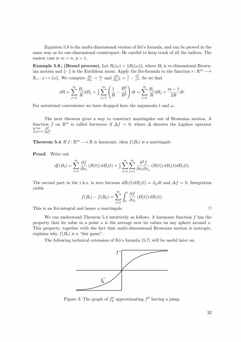
The following technical extension of Ito’s formula (5.7) will be useful later on.

fk"

f "

Figure 3: The graph of f ′′k approximating f ′′ having a jump.

32

Lemma 5.5 Ito’s formula for a function of Brownian motion

f(Bt) = f(B0) +

∫ t

0f ′(Bs) dBs +

12

∫ t

0f ′′(Bs) ds (5.10)

still holds if f : R −→ R is C1 everywhere and C2 outside a finite set z1, . . . , zN , with f ′′bounded on some neighbourhood of this set.

Proof. Take fk ∈ C2(R) such that fk −→ f and f ′k −→ f ′ as k → ∞, both uniformly, andsuch that for x /∈ z1, . . . , zN :

f ′′k (x) −→ f ′′(x) as k → ∞|f ′′k (x)| ≤M in a neighbourhood of z1, . . . , zN .

(Fig. 3 shows the graph of f ′′k approximating some f ′′ with a jump.) For fk we have the Itoformula

fk(Bt) = fk(B0) +

∫ t

0f ′k(Bs)dBs +

12

∫ t

0f ′′k (Bs)ds.

In the limit as k −→ ∞ this equality tends, term by term in L2(Ω,P), to (5.10). Indeed,the distances ∥fk(Bt) − f(Bt)∥ and ∥fk(B0) − f(B0)∥ tend to 0 by the uniformity of theconvergence fk → f , the norm difference ∥

∫ t0 f

′k(Bs) dBs −

∫ t0 f

′(Bs) dBs∥ tends to 0 by theuniformity of the convergence f ′k → f ′ plus Ito’s isometry, and the difference

E(∫ t

0f ′′k (Bs) ds−

∫ t

0f ′′(Bs) ds

)2

≤ t

∫ t

o

∫Ω

(f ′′k (Bs(ω))− f ′′(Bs(ω))

)2P(dω) dstends to 0 by dominated convergence combined with the fact that

P⊗ λ(

(ω, s) ∈ Ω× [0, t] : Bs(ω) ∈ z1, . . . , zN)

= 0.

2

5.4 Local times of Brownian motion

As an application of Lemma 5.5 we shall prove Tanaka’s formula for the local times of Brow-nian motion.

Theorem 5.6 (Tanaka) Let t 7→ Bt be a one-dimensional Brownian motion. Let λ denotethe Lebesgue measure on [0, T ]. Then the limit

Lt := limε↓0

1

2ελ( s ∈ [0, t] : Bs ∈ (−ε, ε)

)exists in L2(Ω,P) and is equal to

Lt = |Bt| − |B0| −∫ t

0sgn(Bs)dBs.

(Think of Lt as the density per unit length of the total time spent close to the origin up totime t.)

33

−ε εFigure 4: The function gε(t).

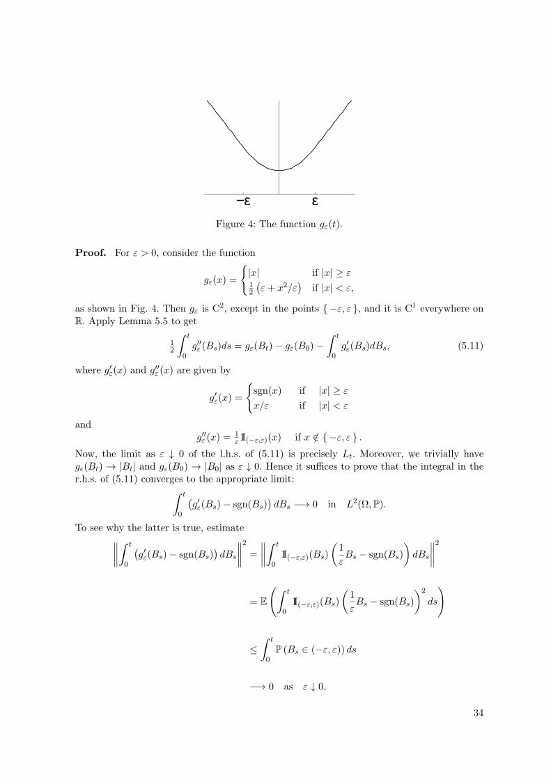
Proof. For ε > 0, consider the function

gε(x) =

|x| if |x| ≥ ε12

(ε+ x2/ε

)if |x| < ε,

as shown in Fig. 4. Then gε is C2, except in the points −ε, ε , and it is C1 everywhere onR. Apply Lemma 5.5 to get

12

∫ t

0g′′ε (Bs)ds = gε(Bt)− gε(B0)−

∫ t

0g′ε(Bs)dBs, (5.11)

where g′ε(x) and g′′ε (x) are given by

g′ε(x) =

sgn(x) if |x| ≥ ε

x/ε if |x| < ε

andg′′ε (x) =

1ε1I(−ε,ε)(x) if x /∈ −ε, ε .

Now, the limit as ε ↓ 0 of the l.h.s. of (5.11) is precisely Lt. Moreover, we trivially havegε(Bt) → |Bt| and gε(B0) → |B0| as ε ↓ 0. Hence it suffices to prove that the integral in ther.h.s. of (5.11) converges to the appropriate limit:∫ t

0

(g′ε(Bs)− sgn(Bs)

)dBs −→ 0 in L2(Ω,P).

To see why the latter is true, estimate∥∥∥∥∫ t

0

(g′ε(Bs)− sgn(Bs)

)dBs

∥∥∥∥2 = ∥∥∥∥∫ t

01I(−ε,ε)(Bs)

(1

εBs − sgn(Bs)

)dBs

∥∥∥∥2

= E

(∫ t

01I(−ε,ε)(Bs)

(1

εBs − sgn(Bs)

)2

ds

)

≤∫ t

0P (Bs ∈ (−ε, ε)) ds

−→ 0 as ε ↓ 0,

34

where in the second equality we use the Ito-isometry, in the inequality we use that |Bs| < εimplies that |ε−1Bs−sgn(Bs)| ≤ 1, and the last statement holds because the Gaussian randomvariable Bs (s > 0) has finite density. It follows that Lt exists and can be expressed as in thestatement of the theorem. 2

Note that for smooth functions f ,

|f(t)| − |f(0)| −∫ t

0sgn (f(s)) f ′(s)ds = 0

becaused

dt|f(t)| = sgn (f(t)) f ′(t) (f(t) = 0).

Thus, the local time is an Ito-correction to this relation, caused by the fact that d|Bt| =sgn (Bt) dBt: if Bt passes the origin during the time interval ∆tj , then |Btj+1 −Btj | need notbe equal to sgn(Btj )∆Btj . The difference is a measure of the time spent close to the origin.

The existence of the local times of Brownian motion was proved by Levy in the 1930’susing hard estimates. The above approach is shorter and more elegant. What is describedabove is the local time at the origin: Lt = Lt(0). In a completely analogous way one can provethe existence of the local time Lt(x) at any site x ∈ R.

The process plays a key role in many applications associated with Brownian motion.For instance, it is used to define path measures that model the behaviour of polymer chains.Let PT denote the Wiener measure on the time interval [0, T ]. Fix a number β > 0, and define

a new measure QβT on path space by setting

dQβT

dPT(·) = 1

ZβT

exp

[−β∫RL2T (x)(·) dx

],

where ZβT is the normalising constant. What the measure Qβ

T does is reward paths thatspread themselves out compared to Brownian motion. We may think of PT as modeling theerratic spatial distribution of the polymer and of the exponential weight factor as modeling itsstiffness or self-repellence. The parameter β is the strength of the self-repellence. It is knownthat

limT→∞

QβT

(|XT |T

∈ [ϑ(β)− ε, ϑ(β) + ε]

)= 1 ∀ε > 0

for some constant ϑ(β), called the asymptotic speed of the polymer, given by

ϑ(β) = Cst · β13 .

(See R. van der Hofstad, F. den Hollander and W. Konig (1997).) The Brownian motioncorresponds to β = 0 and has zero speed.

35

6 Stochastic differential equations

A stochastic differential equation for a process X(t) with values in Rn is an equation of theform

dXi(t) = bi(t,Xt) dt+

m∑j=1

σij(t,Xt) dBj(t) (i = 1, · · · , n). (6.1)

Here, B(t) = (B1(t), B2(t), · · · , Bm(t)) is an m-dimensional Brownian motion, i.e., an m-tuple of independent Brownian motions on R. The functions bi and σij from R×Rn to R withi = 1, 2, . . . , n and j = 1, 2, . . . ,m form a field b of n-vectors and a field σ of n×m-matrices.A process X ∈ L2(B, [0, T ]) for which (6.1) holds is called a strong solution of the equation.In more pictorial language, such a solution is called an Ito-diffusion with drift b and diffusionmatrix σσ∗.

In this section we shall formulate a result on the existence and the uniqueness of Ito-diffusions. It will be convenient to employ the following notation for the norms on vectorsand matrices:

∥x∥2 :=n∑

i=1

x2i (x ∈ Rn); ∥σ∥2 :=n∑

i=1

m∑j=1

σ2ij = tr(σσ∗) (σ ∈ Rn×m).

Also, we would like to take into account an initial conditionX(0) = Z, where Z is an Rn-valuedrandom variable independent of the Brownian motion. All in all, we enlarge our probabilityspace and our space of adapted processes as follows. We choose a probability measure µ onRn and put

Ω′ := Rn × Ωm ;

F ′t := B(Rn)⊗F⊗m

t (t ∈ [0, T ]);

P′ := µ⊗ P⊗m;

Z : Ω′ → Rn : (z, ω) 7→ z;

L2(B, [0, T ])′ := X ∈ L2(Rn, µ)⊗ L2(Ω,FT ,P)⊗m ⊗ L2[0, T ]⊗ Rn |ω 7→ Xx

t,i(ω) is F ′t-measurable.

This change of notation being understood, we shall drop the primes again.

6.1 Strong solutions

Theorem 6.1 Fix T > 0. Let b : [0, T ]×Rn → Rn and σ : [0, T ]×Rn → Rn×m be measurablefunctions, satisfying the growth conditions

∥b (t, x)∥ ∨ ∥σ(t, x)∥ ≤ C (1 + ∥x∥) (t ∈ [0, T ], x ∈ Rn)

as well as the Lipschitz conditions

∥b(t, x)− b(t, y)∥ ∨ ∥σ(t, x)− σ(t, y)∥ ≤ D ∥x− y∥ (t ∈ [0, T ], x, y ∈ Rn),

for some positive constants C and D. Let (Bt)t∈[0,T ] be m-dimensional Brownian motion andlet µ be a probability measure on Rn with

∫Rn ∥x∥2µ(dx) <∞. Then the stochastic differential

equation (6.1) has a unique continuous adapted solution X(t) given that the law of X(0) isequal to µ.

36

Proof. The proof comes in three parts.

1. Uniqueness. Suppose X,Y ∈ L2(B, [0, T ]) are solutions of (6.1) with continuous paths.(Continuity will be proved in part 3). Put

∆bi(t) := bi(t,Xt)− bi(t, Yt)

∆σij(t) := σij(t,Xt)− σij(t, Yt).

Applying the inequality (a + b)2 ≤ 2(a2 + b2) for real numbers a and b, the independenceof the components of B(t), the Cauchy-Schwarz inequality (

∫ t0 g(s)ds)

2 ≤ t∫ t0 g(s)

2ds for anL2-function g, the multi-dimensional Ito-isometry and finally the Lipschitz condition, we find

E(∥Xt − Yt∥2

):=

n∑i=1

E((Xi(t)− Yi(t))

2)

=

n∑i=1

E

∫ t

0∆bi(s)ds+

m∑j=1

∫ t

0∆σij(s)dBj(s)

2≤ 2

n∑i=1

E

(∫ t

0∆bi(s)ds

)2

+

m∑j=1

∫ t

0∆σij(s)dBj(s)

2= 2

n∑i=1

E

((∫ t

0∆bi(s)ds

)2)

+ 2

n∑i=1

E

m∑j=1

∫ t

0(∆σij(s))

2ds

≤ 2t

∫ t

0E

(n∑

i=1

∆bi(s)2

)ds+ 2

∫ t

0E

n∑i=1

m∑j=1

∆σij(s)2

ds

= 2t

∫ t

0E(∥∆b(s)∥2)ds+ 2

∫ t

0E(∥∆σ(s)∥2)ds

≤ 2(t+ 1)D2

∫ t

0E∥Xs − Ys∥2ds.

So the function f : t 7→ E(∥Xt − Yt∥2

)satisfies the integral inequality

0 ≤ f(t) ≤ A

∫ t

0f(s)ds (t ∈ [0, T ]) (6.2)

for the constant A = 2D2(T + 1).

Lemma 6.2 (Gronwall’s lemma) Inequality (6.2) implies that f = 0.

Proof. Put F (t) =∫ t0 f(s)ds. Then F (t) is C

1 and F ′(t) = f(t) ≤ AF (t). Therefore

d

dt

(e−tAF (t)

)= e−tA (f(t)−AF (t)) ≤ 0.

Since F (0) = 0, it follows that e−tAF (t) ≤ 0 implying F (t) ≤ 0. So we have 0 ≤ f(t) ≤AF (t) ≤ 0 and hence f(t) = 0. 2

37

Thus, we have E(∥Xt − Yt∥2

)= 0 for all t ∈ [0, T ]. In particular,

∀t ∈ [0, T ] ∩Q : Xt(ω) = Yt(ω) for almost all ω.

Now letN := ω ∈ Ω | ∃t ∈ [0, T ] ∩Q : Xt(ω) = Yt(ω) .

Then N is a countable union of null sets, so P(N) = 0. For Ω\N we have for all t ∈ [0, T ]∩Q,

Xt(ω) = Yt(ω) ,

and since Xt and Yt have continuous paths we conclude that for almost all ω the equalityextends to all t ∈ [0, T ]. This completes the proof of uniqueness.

2. Existence. We shall find a solution of (6.1) by iterating the map

L2(B, [0, T ]) → L2(B, [0, T ]) : X → X

defined by

Xt = Z +

∫ t

0b(s,Xs)ds+

∫ t

0σ(s,Xs)dBs.

Let us start with the constant process X0t := Z, and define recursively

X(k+1)t := X

(k)t (k ≥ 0).

The calculation in part 1 can be used to conclude that

E(∥∥∥Xt − Yt

∥∥∥2) ≤ A

∫ t

0E(∥Xs − Ys∥2

)ds for any Xs, Ys ∈ L2(B).

Iteration of this result yields, for k ≥ 1 and the choice Xt = X(k)t and Yt = X

(k−1)t ,

E(∥∥∥X(k+1)

t −X(k)t

∥∥∥2) = E(∥∥∥X(k)

t − X(k−1)t

∥∥∥2)≤ A

∫ t

0E(∥∥∥X(k)

s −X(k−1)s

∥∥∥2) ds≤ Ak

∫ t

0dsk−1

∫ sk−1

0dsk−2 · · ·

∫ s1

0ds0 E

(∥∥∥X(1)s0 − Z

∥∥∥2)≤ Aktk

k!K (t ∈ [0, T ]),

where we insert

X(0)s0 = Z +

∫ t

0b(s, Z)ds+

∫ t

0σ(s, Z)dBs

38

and K is given by

K := supt∈[0,T ]

E

(∥∥∥∥∫ t

0b(s, Z)ds+

∫ t

0σ(s, Z)dBs

∥∥∥∥2)

≤ 2 supt∈[0,T ]

E

(∥∥∥∥∫ t

0b(s, Z)ds

∥∥∥∥2)

+ E

(∥∥∥∥∫ t

0σ(s, Z)dBs

∥∥∥∥2)

≤ 2T 2C2E (1 + ∥Z∥)2 + 2TC2E (1 + ∥Z∥)2

≤ 2C2(T 2 + T )E (1 + ∥Z∥)2 ,

which is finite by the growth condition and the requirement that Z has finite variance. Now letX = L2(B, [0, T ]))- limk→∞X(k). The existence of this limit follows because

∑k

√Aktk/k! <

∞ (Cauchy sequence). Then

X =

(L2(B, [0, T ])- lim

k→∞X(k)

)˜= L2(B, [0, T ])- lim

k→∞X(k+1) = X.

So X is a solution of (6.1).

3. Continuity and adaptedness. By Theorem 4.5 the paths t 7→ Xt(ω) can be assumed to becontinuous for almost all ω ∈ Ω. The fact that the solution is adapted is immediate from theconstruction. 2

6.2 Weak solutions

What we have shown in Section 6.1 is that there exists a strong solution of (6.1), i.e., asolution that is an adapted functional of the Brownian motion. In the literature on stochasticdifferential equations often a different point of view is taken, namely one where the Brownianmotion itself is also considered unknown. This leads to a so-called weak solution of stochasticdifferential equations, i.e., a solution in distribution.

Definition. A weak solution of (6.1) is a pair (Bt, Xt), measurable w.r.t. some filtration(Gt)t∈[0,T ] on some probability space (Ω, G, P), such that Bt is m-dimensional Brownianmotion and such that (6.1) holds.

The key point here is that the filtration need not be (Ft)t∈[0,T ] = σ((Bs)s∈[0,t]): if it is,then we have a strong solution.

Definition.

1. Strong uniqueness is uniqueness of a strong solution.

2. Weak uniqueness holds if all weak solutions have the same law.

By the following example we illustrate the difference between these two concepts.

39

Example 6.1.¡ (Tanaka). This example is related to our example of Brownian local time inSection 5.4. Let Bt be a Brownian motion and define

Bt :=

∫ t

0sgn(Bs)dBs.

Since dBt = sgn(Bt)dBt we have, by Ito’s formula in Lemma 5.4,

d(B2t ) = 2BtdBt + (dBt)

2

with (dBt)2 = sgn(Bt)

2(dBt)2 = (dBt)

2 = dt. Hence Bt is a martingale with quadraticvariation t (see Section 2.4):

B2t − 2

∫ t

0BsdBs = t.

Since Bt satisfies the requirements (BM1)–(BM5) of Section 1, it must be a Brownianmotion.

Turning matters around, Bt is itself a solution of the stochastic differential equation

dBt = sgn(Bt)dBt, (6.3)

since Bt =∫ t0 dBs =

∫ t0 sgn(Bs)

2dBs =∫ t0 sgn(Bs)dBs. Because every solution of (6.3) is

a Brownian motion, we have weak uniqueness. However, because −Bt obviously is also asolution of (6.3), there are two solutions of (6.3) for a given process Bt. In other words, wedo not have strong uniqueness.

Taking this argument one step further we find (cf. Theorem 5.6):

B(t) = |B(t)| − |B(0)| − Lt,

where Lt is the local time at the origin. By its definition, Lt is adapted to the filtration

(Gt)t∈[0,T ]

generated by (|Bt|)t∈[0,T ]. Hence so is Bt. It follows that Ft ⊂ Gt, where

(Ft)t∈[0,T ]

is the filtration generated by (Bt)t∈[0,T ]. However, since Bt is not Gt-measurable (its sign is

not determined by Gt), it is not Ft-measurable.

Note that (6.3) is an Ito-diffusion with b(t, x) = 0 and σ(t, x) = sgn(x). The latter isnot Lipschitz, which is why Theorem 6.1 does not apply.

40

7 Ito-diffusions, generators and semigroups

The goal of this section is to give a functional analytic description of Ito-diffusions that willallow us to bring powerful analytic tools into play.

7.1 Introduction and motivation

An Ito-diffusion Xxt (with initial condition Xx

0 = x ∈ Rn) is a Markov process in continuoustime. If we suppose that the field b of drift vectors and the field σ of diffusion matrices are bothtime-independent, i.e., Xx

t is the solution starting at x of the stochastic differential equation

dXt = b(Xt)dt+ σ(Xt)dBt (7.1)

(where b and σ satisfy the growth and the Lipschitz conditions mentioned in Theorem 6.1),then this Markov process is stationary (= time-homogeneous) and can be characterised byits transition probabilities

Pt(x,B) := P [Xxt ∈ B] (t ≥ 0),

where B runs through the Borel subsets of Rn. These transition probabilities satisfy theone-parameter Chapman-Kolmogorov equation

Pt+s(x,B) =

∫y∈Rn

Pt(x, dy)Ps(y,B). (7.2)

An alternative way to characterise an Ito-diffusion is by its action on a sufficiently rich classof functions f : Rn → Rn. Namely, if we define St by

(Stf)(x) := E (f(Xxt )) =

∫y∈Rn

Pt(x, dy)f(y), (7.3)

then (7.2) leads toSt+s = St Ss, (7.4)

i.e., the transformations (St)t≥0 form a one-parameter semigroup. Such a semigroup is deter-mined by its generator A, defined by

Af := limt↓0

1

t(Stf − f) , (7.5)

which describes the action of the semigroup over infinitesimal time intervals. In what followswe make the above observations more precise and we study the interplay between the diffusionXx

t , its generator A and its semigroup (St)t≥0.

7.2 Basic properties

Let t ≥ 0, and for s ≥ t let Xt,xs denote the solution of the stochastic differential equation

(7.1) with initial condition Xt,xt = x.

Lemma 7.1 (Stationarity) The processes s 7→ Xt,xs and s 7→ Xx

s−t are equal in law fors ≥ t.

41

Proof. These processes are solutions of the equations

dXt,xs = b(Xt,x

s )ds+ σ(Xt,xs )d(Bs −Bt)

dXxs−t = b(Xx

s−t)ds+ σ(Xxs−t)d(Bs−t)

respectively, for s ≥ t. Since Bs −Bt and Bs−t are Brownian motions on [t, T ], both startingat 0, the two processes have the same law by weak uniqueness (which is implied by stronguniqueness obtained in Theorem 6.1). 2

Proposition 7.2 (Markov property) Let Xxt (t ≥ 0) denote the solution of (7.1) with

initial condition Xx0 = x. Fix t ≥ 0. Let C0(Rn) be the space of all continuous functions

Rn → R that tend to 0 at infinity. Then for all s ≥ 0 the conditional expectation E(f(Xxt+s)|Ft)

depends on ω ∈ Ω only via Xxt . In fact,

E(f(Xxt+s)|Ft) = (Ssf)(X

xt ).

Proof. Fix t ≥ 0. For y ∈ Rn and s ≥ t, let

Ys(y) := Xt,ys+t.

Then, according to Lemma 7.1, Ys(y) and Xys have the same law. Hence, for all f ∈ C0(Rn),

E (f(Ys(y))) = E (f(Xys )) = (Ssf)(y).

On the other hand, the random variable Ys(y) depends on ω ∈ Ω only via the Brownianmotion u 7→ Bu(ω)−Bt(ω) for u ≥ t, so Ys(y) is stochastically independent of Ft. By stronguniqueness we must have, for s ≥ 0,

Ys (Xxt ) = Xx

t+s a.s.,

since both sides are solutions of the same stochastic differential equation (7.1) for s ≥ 0 withinitial condition Y0(X

xt ) = Xx

t . As Xxt is Ft-measurable, we now have

E(f(Xx

t+s|Ft))(ω) =

∫ω′∈Ω

f(Ys(X

xt (ω))(ω

′))P(dω′) = (Ssf) (X

xt (ω)) ,

where ω represents the randomness before time t and ω′ the randomness after time t. 2

Definition. Let B be a Banach space. A jointly continuous one-parameter semigroup ofcontractions on B is a family (St)t≥0 of linear operators St : B → B satisfying the followingrequirements:

CS1. ∥Stf∥ ≤ ∥f∥ for all t ≥ 0, f ∈ B;CS2. S0f = f for all f ∈ B;CS3. St+s = St Ss for all t, s ≥ 0;CS4. the map (t, f) 7→ Stf is jointly continuous [0,∞)× B → B.

42

We choose B = C0(Rn). The natural norm on this space is the supremum norm

∥f∥ := supx∈Rn

|f(x)|.

For f ∈ C0(Rn) we define(Stf)(x) := E (f(Xx

t )) ,

where Xxt (t ≥ 0) denotes the solution of (7.1) with initial condition Xx

0 = x.

Theorem 7.3 The operators St with t ≥ 0 form a jointly continuous one-parameter semi-group of contractions C0(Rn) → C0(Rn).

Proof. We prove properties 1–4 in Definition 7.2.

1. Fix t ≥ 0 and f ∈ C0(Rn). We show that the function Stf again lies in C0(Rn), by showingthat it is continuous and tends to 0 at infinity. The inequality ∥Stf∥ ≤ ∥f∥ is obvious fromthe definition of St.

Continuity: Choose x, y ∈ Rn and consider the processes Xxt and Xy

t . The basic estimate inSection 6.1 yields

E∥Xxt −Xy

t ∥2 ≤ 2

(∥x− y∥2 +A

∫ t

0E∥Xx

s −Xys ∥2ds

)for some constant A. Putting F (t) :=

∫ t0 E∥X

xs −Xy

s ∥2ds, we may write this as

d

dtF (t) ≤ 2∥x− y∥2 + 2AF (t).

Sod

dt

(e−2AtF (t)

)≤ 2∥x− y∥2e−2At.

Hence, as F (0) = 0,

e−2AtF (t) ≤ ∥x− y∥2 1A

(1− e−2At

),

orAF (t) ≤ ∥x− y∥2

(e2At − 1

).

We thus obtain that

E∥Xxt −Xy

t ∥2 ≤ 2∥x− y∥2 + 2AF (t) ≤ 2∥x− y∥2e2At. (7.6)

Now choose ε > 0. Since f is uniformly continuous on Rn, there exists a δ′ > 0 such that

∀x′, y′ ∈ Rn : ∥x′ − y′∥ ≤ δ′ =⇒ |f(x′)− f(y′)| ≤ ε

2.

43

It follows that for x, y ∈ Rn not more than δ := δ′√εe−At/2

√2∥f∥ apart we may estimate∣∣∣(Stf)(x)− (Stf)(y)

∣∣∣ = ∣∣∣E(f(Xxt ))− E(f(Xy

t ))∣∣∣

≤ E |f(Xxt )− f(Xy

t )|

≤ ε

2+ 2∥f∥ P

[∥Xx

t −Xyt ∥ > δ′

]≤ ε

2+ 4∥f∥ 1

(δ′)2e2At∥x− y∥2

< ε,

where the third inequality uses the Markov inequality and (7.6). We conclude that Stf isuniformly continuous as well.

Approach to 0 at infinity : It suffices to prove that there exists a τ > 0 such that for allt ∈ [0, τ ] we have

lim∥x∥→∞

(Stf)(x) = 0.

Indeed, the same then holds for all t by the semigroup property. Heuristically speaking, wemust prove that the diffusion cannot escape to infinity in a finite time. We start with theestimate

E∥∥∥Xx,(k+1)

t −Xx,(k)t

∥∥∥2 ≤ Aktk

k!Dt(1 + ∥x∥)2

for the iterates of the map X 7→ X in Section 6.1, starting from the constant process Xx,0t = x.

Since Xxt = x+

∑k(X

x,(k+1)t −Xx,(k)) (because (X

x,(k)t → Xx

t as k → ∞), it follows that

E ∥Xxt − x∥2 ≤ Dt(1 + ∥x∥)2 (7.7)

with Dt = Dt(∑

k

√Aktk/k!)2. Now choose ε > 0. Let M > 0 be such that |f(x′)| ≤ ε

2 forall x′ ∈ Rn with ∥x′∥ ≥M , and let τ > 0 be such that 16Dτ∥f∥ < 1

2ε. Then, by the triangleinequality in Rn and by Chebyshev’s inequality, we have for all x ∈ Rn with ∥x∥ > 2M ∨ 1and all t ∈ [0, τ ]:

∥(Stf)(x)∥ ≤ ε

2+ ∥f∥ P [∥Xx

t ∥ < M ]

≤ ε

2+ ∥f∥ P

[∥Xx

t − x∥ > 12∥x∥

]≤ ε

2+ ∥f∥ 4

∥x∥2E∥Xx

t − x∥2

≤ ε

2+ ∥f∥ 4

∥x∥2Dτ (1 + ∥x∥)2

≤ ε

2+ ∥f∥ 4Dτ

(1

∥x∥+ 1

)2

< ε.

Since ε is arbitrary, this proves the claim.

2. From the initial condition Xx0 = x it is obvious that (S0f)(x) = E (f(Xx

0 )) = f(x).

44

3. The semigroup property of St is a consequence of the Markov property of Xt. Namely, forall s, t ≥ 0 and all x ∈ Rn:

(St+sf) (x) = E(f(Xx

t+s

))= E

(E(f(Xx

t+s

)|Ft

))= E ((Ssf) (X

xt ))

= (St (Ssf)) (x) .

4. To prove the joint continuity of the map (t, f) 7→ Stf , it in fact suffices to show thatStf −→ f as t ↓ 0. Indeed, for all s > t ≥ 0,

∥Stf − Ssg∥ = ∥St(f − Ss−tg)∥ ≤ ∥f − Ss−tg∥ ≤ ∥f − g∥+ ∥g − Ss−tg∥.

Note that from (7.7) it follows that limt↓0 E∥Xxt −x∥2 = 0. Now again take ε > 0. Let δ > 0 be

such that ∥x−y∥ < δ =⇒ |f(x)−f(y)| < ε/2. Let t0 > 0 be such that E∥Xxt −x∥2 < εδ2/4∥f∥

for 0 ≤ t ≤ t0. Then for t ∈ [0, t0] we have, again by Chebyshev’s inequality,

|(Stf) (x)− f (x)| =∣∣∣∣∫

Ω(f (Xx

t (ω))− f(x))P (dω)

∣∣∣∣≤ ε

2+ 2 ∥f∥P [∥Xx

t (ω)− x∥ ≥ δ]

≤ ε

2+

2∥f∥δ2

E∥Xxt − x∥2

< ε.

2

7.3 Generalities on generators

We next describe some basic theory for one-parameter semigroups on Banach spaces. (Werefer to the book of E.B. Davies (1980) for further details.)

Definition. The domain of a generator A of a one-parameter semigroup (St)t≥0 on a Banachspace B is defined by

Dom(A) :=

f ∈ B

∣∣∣∣limt↓0 1t (Stf − f) exists

,

and for f in this domain, Af denotes the limit.

This definition leads to the following.

Proposition 7.4 Let A be the generator of a jointly continuous one-parameter semigroup(St)t≥0 on a Banach space B. Then

(i) Dom(A) is dense in B;(ii) St leaves Dom(A) invariant: St(Dom(A)) ⊂ Dom(A);(iii) ∀f ∈ Dom(A) : StAf = AStf = d

dtStf .

45

Proof. (i). For f ∈ B and ε > 0 we define

fε :=1

ε

∫ ε

0Stfdt.

Then limε↓0 fε = f , so fε|ε > 0, f ∈ B is dense in B. But we also have

1

h(Sh − 1I) fε =

1

h(Sh − 1I)

1

ε

∫ ε

0Stfdt

=1

hε

(∫ h+ε

hStfdt−

∫ ε

0Stfdt

)=

1

hε

(∫ h

0St(Sεf)dt−

∫ h

0Stfdt

)−→ 1

ε(Sεf − f) as h ↓ 0.

So fε ∈ Dom(A), and hence Dom(A) is dense in B.

(ii),(iii). If f ∈ Dom(A), then

1

h(Sh − 1I) (Stf) = St

(1

h(Sh − 1I) (f)

)→ StAf, as h ↓ 0.

So Stf ∈ Dom(A) and AStf = StAf . The identity AStf = ddtStf follows from the definition

of A. 2

Since St is the solution of the differential equation ddtStf = AStf with initial condition

S0 = 1I, it is customary to writeSt = etA.

The next theorem gives us an explicit formula for the generator of an Ito-diffusion ona large subset of its domain (namely, all functions that are twice continuously differentiableand have compact support).

Theorem 7.5 Let (St)t≥0 be the one-parameter semigroup on C0(Rn) associated to an Ito-diffusion with coefficients b and σ. Let A be the generator of (St)t≥0. Then C

2c (Rn) ⊂ Dom(A),

and for all f ∈ C2c (Rn):

(Af)(x) =∑i

bi(x)∂f

∂xi(x) + 1

2

∑i,j

(σ(x)σ(x)∗)ij∂2f

∂xi∂xj(x). (7.8)

Proof. Denote the r.h.s. of (7.8) by A′f . By Ito’s formula we have

df(Xt) =∑i

∂f

∂xi(Xt) dXi(t) +

12

∑i,j

∂2f

∂xi∂xj(Xt) dXi(t)dXj(t).

Since dXi(t) = bi (Xt) dt+∑

j σij(Xt)dBj(t), we have

dXidXj =

(∑k

σikdBk

)(∑l

σjldBl

)=

(∑k

σikσjk

)dt = (σσ∗)ij dt.

46

Using the condition Xx0 = x, we conclude that for any f ∈ C2

c (Rn),

f (Xxt )− f(x) =

∫ t

0

∑i,j

∂f

∂xi(Xx

s )σij (Xxs ) dBj(s) +

∫ t

0

(A′f

)(Xx

s ) ds. (7.9)

The first part on the r.h.s. is a martingale and therefore

(Af) (x) = limt↓0

1t (E (f (Xx

t ))− f (x)) = limt↓0

E(

1t

∫ t

0

(A′f

)(Xx

s ) ds

). (7.10)

Since A′f is a continuous function, we have almost surely

limt↓0

1

t

∫ t

0(A′f)(Xx

s ) ds −→ (A′f)(x) ,

and since A′f is bounded we can apply dominated convergence to the r.h.s. of (7.10) andconclude that (Af)(x) = (A′f)(x). 2

Theorem 7.5 shows that on C2c (Rn) the generator A acts as a second-order differential

operator, with a first-order part coming from the drift and a second-order part coming fromthe diffusion. This fundamental fact forms a bridge between the theory of partial differentialequations and the study of diffusions.

In general it is difficult to calculate the evolution semigroup St, but in a few exceptionalcases, such as that of the Ornstein-Uhlenbeck process, the differential equation d

dtSt = StAcan be explicitly solved.

Proposition 7.6 Let η and σ be positive numbers, and let (St)t≥0 be the semigroup ofcontractions C0(R) → C0(R) associated to the stochastic differential equation

dXt = −ηXt dt+ σ dBt . (7.11)

Then for all f ∈ C0(R) an x ∈ R,

(Stf)(x) =1

σ

√η

π(1− e−2ηt)

∫ ∞

−∞exp

(−η(xe

−ηt − y)2

σ2(1− e−2ηt)

)f(y) dy .

Exercise Prove this proposition by checking explicitly that for all t ≥ 0

d

dtStf = St(Af) ,

where A is the generator of the Ornstein-Uhlenbeck process, given for f ∈ C20 (R) by

Af(x) := −ηxf ′(x) + 12σ

2f ′′(x) .

Below we shall give a stochastic proof.

47

Proof. First note that the solution Xxt of (7.11) with initial condition Xx

0 = x is given by

Xxt = xe−ηt + σNft ,

where ft(x) = 1[0,t](x)eη(x−t). (Cf. (3.3).) For t ≥ 0, let γt denote the Gaussian density with

mean 0 and variance σ2∥ft∥2 = σ2(1− e−2ηt)/2η, and for f ∈ C20 (R), let f denote the Fourier

transform of f , so that

f(x) =1

2π

∫ ∞

−∞eiωxf(ω) dω ,

Then, since E(eiωσNft ) = γt(ω), we have, using Fubini’s theorem and the property that theFourier transform of a convolution product equals the product of the Fourier transforms,

(Stf)(x) = E(f(Xx

t ))

=1

2πE(∫ ∞

−∞eiωX

xt f(ω)dω

)=

1

2π

∫ ∞

−∞E(eiωxe

−ηt+iωσNft

)f(ω) dω

=1

2π

∫ ∞

−∞eiωxe

−ηtγt(ω)f(ω) dω

=

∫ ∞

−∞γt(xe

−ηt − y)f(y) dy .

(7.12)

By writing out the function γt we obtain the statement. 2

7.4 Dynkin’s formula and applications

Having thus identified the generator associated with Ito-diffusions, we next formulate animportant formula for stopped Ito-diffusions. A stopping time τ for (Xx

t )t≥0 is a randomvariable such that for all t ≥ 0 the event [τ ≤ t] := ω ∈ Ω|τ(ω) ≤ t is an element of thesigma-algebra Ft generated by (Xx

s )s∈[0,t].

Theorem 7.7 (Dynkin’s formula) Let X be a diffusion in Rn with generator A. Let τ bea stopping time with E(τ) <∞. Then for all f ∈ C2

c (Rn) and all x ∈ Rn,

Ex (f (Xτ )) = f (x) + Ex

(∫ τ

0(Af) (Xs) ds

).

Proof. The theorem is intuitive, but its proof is rather technical. We limit ourselves here toa very brief sketch.

By applying (7.9) to the stopped process t 7→ Xxt∧τ and letting t tend to infinity after-

wards, we find:

f (Xxτ ) = f (x) +

∫ τ

0

∑i,j

∂f

∂xi(Xx

s )σij(Xxs )dBj(s) +

∫ τ

0(Af) (Xx

s ) ds.

48

After taking expectations we get the statement, since stopped martingales starting at 0 haveexpectation 0. (See Dynkin (1963).) 2

The simplest example of a diffusion is Brownian motion itself: Xt = Bt (b ≡ 0, σ ≡ id).Its generator is 1/2 times the Laplacian ∆. We investigate two problems.

Example 7.1.¡ Consider Brownian motion Bat := a + Bt starting at a ∈ Rn. Let R > ∥a∥.

What is the average time Bat spends inside the ball DR = x ∈ Rn : ∥x∥ ≤ R ?

Solution: Choose f ∈ C2c (Rn) such that f(x) = ∥x∥2 for ∥x∥ ≤ R. Let τaR denote the first

time the Brownian motion hits the sphere ∂DR. Then τaR is a stopping time. Put τ := τaR ∧ T

and apply Dynkin’s formula, to obtain

E (f(Baτ )) = f(a) + E

(∫ τ

0

12 (∆f) (B

as ) ds

)= ∥a∥2 + nE(τ),

where we use that 12∆f ≡ n. Obviously, E (f(Ba

τ )) ≤ R2. Therefore

E(τ) ≤ 1n

(R2 − ∥a∥2

).

As this holds uniformly in T , it follows that E(τaR) ≤1n

(R2 − ∥a∥2

)< ∞. Hence τ → τaR as

T → ∞ by monotone convergence. But then we must have f(Baτ ) → ∥Ba

τaR∥2 = R2 as T → ∞,

and so in factE (τaR) =

1n

(R2 − ∥a∥2

)by dominated convergence.

Example 7.2.¡ Let b ∈ Rn be a point outside the ball DR. What is the probability that theBrownian motion starting in b ever hits ∂DR?

Solution: We cannot use Dynkin’s formula directly, because we do not know whether theBrownian motion will ever hit ∂DR (i.e., whether τ < ∞). In order to obtain a well-definedstopping time, we need a bigger ball DM := x ∈ Rn|∥x∥ ≤M enclosing the point b. LetσbM,R be the first exit time from the annulus AM,R := DM\DR starting from b. Then clearly

σbM,R = τ bM ∧ τ bR. Now take A = 12∆, the generator of Brownian motion, and suppose that

fM,R : AM,R → Rn satisfies the following requirements:

(i) ∆fM,R = 0, i.e., fM,R is harmonic,(ii) fM,R(x) = 1 for ∥x∥ = R,(iii) fM,R(x) = 0 for ∥x∥ =M .

We then findP[∥∥∥Bb

σbM,R

∥∥∥ = R]= E

[fM,R

(Bb

σbM,R

)]= fM,R(b),

where the first equality uses (ii) and (iii) and the second equality uses Dynkin’s formula incombination with (i). Incidentally, this equation says that fM,R is uniquely determined if itexists.

49

Next, we let M → ∞ to obtain

P[τ bR <∞

]= P

[∃M ≥ ∥b∥ : τ bR < τ bM

],

because any path of Brownian motion that hits ∂DR must be bounded. From the latter wein turn obtain

P[τ bR <∞

]= P

(∪M≥∥b∥[τ

bR < τ bM ]

)= lim

M→∞P[τ bR < τ bM

]= lim

M→∞P[∥∥∥Bb

σbM,R

∥∥∥ = R]= lim

M→∞fM,R(b).

Thus, the only thing that remains to be done is to calculate this limit, i.e., we must solve(i)-(iii).

For n = 2 we find, after some calculation:

fM,R(b) =log ∥b∥ − logM

logR− logM→ 1 as M → ∞.

For n = 2, on the other hand, we find:

fM,R(b) =∥b∥2−n −M2−n

R2−n −M2−n→

1 if n = 1

(∥b∥/R)2−n if n ≥ 3.

It follows that Brownian motion with n = 1 or n = 2 is recurrent, since it will hit any spherewith probability 1. But for n ≥ 3 Brownian motion is transient.

50

8 Transformations of diffusions

In this section we treat two formulas from the theory of diffusions, both of which describeways to transform diffusions and are proved using Ito-calculus.

8.1 The Feynman-Kac formula

Theorem 8.1 (Feynman-Kac formula) For x ∈ Rn, let Xxt be an Ito-diffusion with gen-

erator A and initial condition Xx0 = x. Let v : Rn → [0,∞) be continuous, and let Sv

t f forf ∈ C0(Rn) and t ≥ 0 be given by

(Svt f) (x) = E

(f (Xx

t ) exp

(−∫ t

0v(Xx

u)du

)).

Then (Svt )t≥0 is a jointly continuous semigroup on C0(Rn) (in the sense of Definition 7.2)

with generator A− v.

Proof. It is not difficult to show, by the techniques used in the proof of Theorem 7.3, thatSvt f lies again in C0(Rn), and that the properties 1, 2 and 4 in Definition 7.2 hold (note thatv is non-negative). It is illuminating, however, to explicitly prove Property 3.

For 0 ≤ s ≤ t, let

Zxs,t := exp

(−∫ t

sv (Xs,x

u ) du

).

Property 3 in Definition 7.2 is preserved due to the particular form of the process Zx0,t. In

fact, let f ∈ C0(Rn). Then(Svt+sf

)(x) = E

(Zx0,t+sf

(Xx

t+s

))= E

(Zx0,tZ

Xxt

t,t+sf(Xx

t+s

))= E

(Zx0,tE

(Z

Xxt

t,t+sf(X

t,Xxt

t+s

)|Ft

))= E

(Zx0,tg (X

xt ))

= (Svt g) (x) ,

whereg(y) = E

(Zyt,t+sf(X

t,yt+s)|Ft

)= E

(Zy0,sf(X

ys ))= (Sv

s f)(y)

by stationarity. So indeed (Svt+sf

)(x) = (Sv

t Svs f) (x) .

Let us finally show that A − v is the generator of (Svt )t≥0. To that end we calculate

(dropping the upper index x):

d (Z0,tf (Xt)) = f (Xt) dZ0,t + Z0,tdf (Xt)

=[−v (Xt) f (Xt) + (Af) (Xt)

]Z0,tdt+ Z0,t⟨σ (Xt)

T ∇f (Xt) , dBt⟩.(8.1)

51

Here we use Ito’s formula and dXt = b(Xt)dt+ σ(Xt)dBt to compute

df (f(Xt)) =∑i

∂f

∂xi(Xt)dXi(t) +

1

2

∑i,j

∂2f

∂xi∂xj(Xt)dXi(t)dXj(t)

=∑i

∂f

∂xi(Xt)bi(Xt)dt+

∑i,j

∂f

∂xi(Xt)σij(Xt)dBj(t)

1

2

∑i,j

∂2f

∂xi∂xj(Xt)(σσ

∗)ij(Xt)dt,

(8.2)

where the first and third term are precisely (Af)(Xt)dt according to Theorem 7.5. Takingexpectations on both sides of (8.1), we get

dE (Z0,tf (Xt)) = E ([−vf +Af ] (Xt)Z0,tdt) .

In short, d(Svt f) = Sv

t ((A− v)f) dt, which means that A − v is indeed the generator of thesemigroup (Sv

t )t≥0 (recall Proposition 7.4(iii)). 2

We can give the semigroup (Svt )t≥0 a clear probabilistic interpretation. The positive

number v(y) is viewed as a “hazard rate” at y ∈ Rn, the probability per unit time for thediffusion process to be “killed”. Let us extend the state space Rn by a single point ∂, the“coffin” state, where the system ends up after being killed. Then it can be shown that thereexists a stopping time τ , the “killing time”, such that the process Y x

t given by

Y xt :=

Xx

t if t ≤ τ

∂ if t > τ

satisfies

E (f (Y xt )) = E

(f (Xx

t ) exp

(−∫ t

0v (Xx

u) du

)),

provided we define f(∂) := 0. The proof of this requires an explicit construction of the killingtime τ , which we shall not give here.

Example 8.1.¡ The Feynman-Kac formula was originally formulated as a non-rigorous “path-integral formula” in quantum mechanics by R. Feynman, and was later reformulated in termsof diffusions by M. Kac. The connection with quantum mechanics can be stated as follows. IfXt is Brownian motion, then the generator of (Sv

t )t≥0 is 12∆− v. This is (−1)× the Hamilton

operator of a particle in a potential v in Rn. According to Schrodinger, the evolution in timeof the wave function ψ ∈ L2(Rn) describing such a particle is given by ψ 7→ Uv

t ψ, where Uvt

is a group of unitary operators given by

Uvt = exp

(it(12∆− v

))(t ∈ R).

This group can be obtained by analytic continuation in t into the complex domain of thesemigroup

Svt = exp

(t(12∆− v

))(t ∈ [0,∞)).

52

Example 8.2.¡ Consider the partial differential equation

∂

∂tu(x, t) = ∆u(x, t) + ξ(x)u(x, t), x ∈ Rd, t ≥ 0, (8.3)

with initial conditionsu(x, 0) = 1 ∀x ∈ Rd. (8.4)

Here, ∆ is the Laplacian acting on the spatial variable and ξ(x) : x ∈ Rd is a field of randomvariables that plays the role of a random medium. Depending on the choice that is made forthe probability law of this random field, (8.3) can be used in various areas of chemistry andbiology. For instance, u(x, t) describes the flow of heat in a medium with randomly locatedsources and sinks.

A formal solution of (8.3) and (8.4) can be written down with the help of the Feynman-Kac formula:

u(x, t) = E(exp

[∫ t

0ξ(Bx

s ) ds

]).

This representation expresses u(x, t) in terms of a Brownian motion starting at x and is thestarting point for a detailed analysis of the behaviour of the random field u(x, t) : x ∈ Rdas t→ ∞. (See Carmona and Molchanov (1994)).

Finally, if v fails to be nonnegative, then the Feynman-Kac formula may still hold. Forinstance, it suffices that v be bounded from below. This guarantees that the properties inDefinition 7.2 hold.

8.2 The Cameron-Martin-Girsanov formula

Brownian motion starting at x ∈ Rn can be represented naturally on the probability space(Ω,F ,Px), where Ω = C([0, T ] → Rn) is the space of its paths, F is the σ-algebra generatedby the cylinder sets ω ∈ Ω | a ≤ ω(t) ≤ b (a, b ∈ R, t ∈ [0, T ]), and Px is the probabilitydistribution on C[0, t] of (Bx

t := x+Bt)t∈[0,T ] constructed in Section 2. We want to comparethe probability distribution Px with that of another process derived from it, namely, Brownianmotion with a drift.

Let Xxt denote the solution of

dXxt = b (Xx

t ) dt+ dBt, Xx0 = x, (8.5)

where b is bounded and Lipschitz continuous. The process Xxt induces a probability measure

Pxb on Ω.

Theorem 8.2 (Cameron-Martin-Girsanov formula) For all x ∈ Rn the probability mea-sures Px and Px

b are mutually absolutely continuous with Radon-Nikodym derivative givenby

dPxb

dPx

((Bx

s )s∈[0,T ]

)= exp

(∫ T

0⟨b (Bx

s ) , dBxs ⟩ − 1

2

∫ T

0∥b (Bx

s )∥2 ds

).

Proof. Fix x ∈ Pn. The idea of the proof is to show that Xxt has the same distribution

under Px as Bxt has under ρTPx, where ρT denotes the Radon-Nikodym derivative of the

53

theorem. In other words, we shall show that for all 0 ≤ t1 ≤ t2 ≤ · · · ≤ tn ≤ T and allf1, f2, . . . fn ∈ C0(Rn):

Ex (f1(Xt1)× · · · × fn(Xtn)) = Ex(ρT f1

(Bx

t1

)× · · · × fn

(Bx

tn

)). (8.6)

Indeed, by the definition of Pxb the l.h.s. is equal to∫Ωf1(ω(t1))× · · · × fn(ω(tn))Px

b (dω)

and the r.h.s. is equal to∫Ωf1 (ω(t1))× · · · × fn (ω(tn)) ρT (ω)Px (dω) ,

while the functions ω 7→ f1 (ω(t1))×· · ·× fn (ω(tn)) generate the σ-algebra F when t1, . . . , tnare running. We shall prove (8.6) by showing that both sides are equal to

St1(f1 St2−t1

(· · ·Stn−tn−1(fn) · · ·

))(x). (8.7)

Let us start with the l.h.s. of (8.6). First we note that, for all 0 ≤ s ≤ t ≤ T , all F inthe algebra As of bounded Fs-measurable functions on Ω and all f ∈ C0(Rn), by the propertyof conditional expectations and the Markov property we have that

Ex(F f(Xt)) = Ex(E(F f(Xt))|Fs

)= Ex

(F E(f(Xt))|Fs

)= Ex

(F (St−sf)(Xs)

).

If we apply this result repeatedly to the product f1(Xt1)×· · ·× fn(Xtn), first projecting ontoAtn−1 , then onto Atn−2 , and all the way down to At1 , then we obtain (8.7).

Next consider the r.h.s. of (8.6), which is more difficult to handle. We shall show thatit is also given by (8.7), in three steps:

Step 1. For all 0 ≤ t ≤ T and F ∈ At:

Ex (FρT ) = Ex (Fρt) . (8.8)

Hence the r.h.s. of (8.6) does not depend on T (as long as T ≥ tn).

Step 2. For all 0 ≤ s ≤ T , F ∈ As and f ∈ C0(Rn):

Ex (F f (Bt) ρT ) = Ex (F (St−sf)(Bs)ρT ) . (8.9)

Step 3. We apply (8.9) repeatedly, first with t = tn, s = tn−1, F ∈ Atn−1 , then with t = tn−1,s = tn−2, F ∈ Atn−2 , continuing all the way down to t = t1, and we obtain (8.7).

Thus, to complete the proof it remains to prove (8.8) and (8.9).

Proof of 1. Put ρt := exp (Zt) with

dZt = ⟨b (Bt) , dBt⟩ − 12 ∥b (Bt)∥2 dt.

54

Then ρT is as defined above and Ito’s formula gives

dρt = exp (Zt) dZt +12 exp (Zt) (dZt)

2 = ρt⟨b (Bt) , dBt⟩,

where two terms cancel because (dZt)2 = ∥b(Bt)∥2. It follows that t 7→ ρt is a martingale.

Therefore, for F ∈ At,

Ex (FρT ) = Ex (E (FρT |Ft))

= Ex (FE (ρT |Ft))

= Ex (Fρt) .

Proof of 2: Note that, by Ito’s formula,

d (ρtf (Bt)) = f (Bt) dρt + ρtdf(Bt) + (dρt)(df(Bt))

= ρt

(f(Bt)⟨b (Bt) , dBt⟩+ ⟨∇f (Bt) , dBt⟩

)+ ρt

(12∆f (Bt) dt+ ⟨b (Bt) ,∇f (Bt)⟩dt

)following a calculation similar to (8.1) and (8.2). Hence, for 0 ≤ s ≤ t (with F ∈ As) we have,by (8.8),

d

dtEx (FρT f (Bt)) =

d

dtEx (Fρtf (Bt))

= Ex (Fρt (Af) (Bt))

= Ex (F (Af) (Bt) ρT ) ,

where A := 12∆ + ⟨b,∇⟩ is the generator of (Xt). Therefore the l.h.s. and the r.h.s. of (8.9)

have the same derivative with respect to t for any t ≥ s ≥ 0. Since they are equal for t = s,they must be equal for all t ≥ s ≥ 0. 2

The Cameron-Martin-Girsanov formula is a generalisation by Girsanov (1960) of theoriginal formula of Cameron and Martin (1944) for a translation in Wiener space, which wenow give as a special case. Let h be a square integrable function [0, T ] → R, and consider theshifted noise N given by

Nf := ⟨h, f⟩+Nf .

Clearly this corresponds to a shift in the associated Brownian motion given by

Bt =

∫ t

0h(s)ds+Bt .

Now, since this shifted Brownian motion satisfies the stochastic differential equation

dBt = h(t) dt+ dBt ,

the Cameron-Martin-Girsanov formula says that the probability distributions P and P arerelated by

dPdP

= exp

(∫ T

0h(t) dBt − 1

2

∫ T

0h(t)2 dt

)= eNh− 1

2∥h∥2 .

55

This Radon-Nikodym derivative can be understood as a quotient of Gaussian densities, asthe following analogy shows. Let γ be the standard Gaussian density on the real line, and γµis its translate over a distance µ ∈ R, then

γµ(x)

γ(x)=e−

12(x−µ)2

e−12x2

= e2µx−12µ2.

56

9 The linear Kalman-Bucy filter

The Kalman-Bucy filter is an algorithm that filters out random errors occurring in the ob-servation of a stochastic process. When put on a fast computer, the algorithm follows theobservations in “real time”: at each moment it produces the best possible estimate of theactual value of the process under observation (given certain probabilistic assumptions on theprocess itself and on the observation errors).

The filter is called “linear” because the estimates depend linearly on the observations.In fact, the model on which the algorithm is based is situated in a Hilbert space of jointlyGaussian random variables with mean zero. In such a space independence is equivalent toorthogonality. For the general nonlinear theory of stochastic filtering we refer to the book ofKallianpur (1980).

The basic idea of linear filtering is best understood by a simple example. From therewe shall build up the full model of Kalman and Bucy.

9.1 Example 1: observation of a single random variable

Let X be a Gaussian random variable with mean 0 and variance a2. Suppose that we cannotobserve X directly, but only with some small Gaussian error W , independent of X, that hasmean 0 and variance m2. So we observe

Z := X +W.

We are interested in the best estimate X of X based on our observation of Z and the aboveassumptions. It is reasonable to interpret “best” as the requirement that E((X − X)2) beminimal, which leads to

X := E (X|F (Z)) ,

i.e., the orthogonal projection of X onto L2 (Ω,F (Z) ,P), where F (Z) is the σ-algebra gen-erated by Z. This is equivalent to projecting X onto the one-dimensional space RZ.

Proposition 9.1 The best estimate of X is given by (see Fig. 5)

X =E (XZ)

E (Z2)Z =

a2

a2 +m2Z.

Proof. Put

Y :=a2

a2 +m2Z.

Then, because E(XW ) = 0,

E((X − Y )Z

)= E

((m2X − a2W

a2 +m2

)(X +W

))= 0.

So (X − Y ) ⊥ Z. For jointly Gaussian random variables with mean zero, orthogonality (i.e.,absence of correlation) implies independence. So (X−Y ) ⊥⊥ Z. It follows that X−Y ⊥⊥ F forall F ∈ L2(Ω,F(Z),P), and since Y ∈ L2(Ω,F(Z),P) it follows that Y = E(X|F(Z)) =: X(see Fig. 5). 2

57

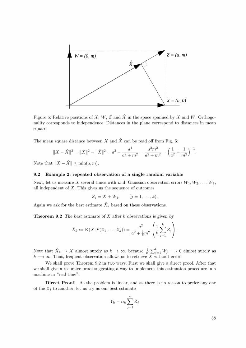
W = (0, m) Z = (a, m)

X^

X = (a, 0)

Figure 5: Relative positions of X, W , Z and X in the space spanned by X and W . Orthogo-nality corresponds to independence. Distances in the plane correspond to distances in meansquare.

The mean square distance between X and X can be read off from Fig. 5:

∥X − X∥2 = ∥X∥2 − ∥X∥2 = a2 − a4

a2 +m2=

a2m2

a2 +m2=( 1

a2+

1

m2

)−1.

Note that ∥X − X∥ ≤ min(a,m).

9.2 Example 2: repeated observation of a single random variable

Next, let us measure X several times with i.i.d. Gaussian observation errors W1,W2, . . . ,Wk,all independent of X. This gives us the sequence of outcomes

Zj = X +Wj , (j = 1, · · · , k).

Again we ask for the best estimate Xk based on these observations.

Theorem 9.2 The best estimate of X after k observations is given by

Xk := E (X|F(Z1, . . . , Zk)) =a2

a2 + 1km

2

1

k

k∑j=1

Zj

.

Note that Xk → X almost surely as k → ∞, because 1K

∑kj=1Wj −→ 0 almost surely as

k −→ ∞. Thus, frequent observation allows us to retrieve X without error.

We shall prove Theorem 9.2 in two ways. First we shall give a direct proof. After thatwe shall give a recursive proof suggesting a way to implement this estimation procedure in amachine in “real time”.

Direct Proof. As the problem is linear, and as there is no reason to prefer any oneof the Zj to another, let us try as our best estimate

Yk = αk

k∑j=1

Zj

58

for some constant αk. Again, we require E((X − Yk)Zi) = 0 (i = 1, . . . , k). So, becauseE(XZi) = E(X2) = a2,

0 = E ((X − Yk)Zi) = E

X − αk

k∑j=1

Zj

Zi

= a2 − αk

k∑j=1

E (ZiZj) .

Now

E(ZiZj) = E((X +Wi)(X +Wj)

)=

a2 if i = j;

a2 +m2 if i = j,

which givesk∑

j=1

E(ZiZj) = ka2 +m2.

Using this result we obtain

αk =a2

ka2 +m2=

1

k

a2

a2 + 1km

2.

Therefore Yk = Xk if αk is given the above value. 2

Recursive Proof. The goal of this proof is to find a recurrence relation in k for Xk.This is done by means of a procedure that is essential to linear filtering: one identifies whatis new in each of the consecutive observations by means of the so-called innovation process(Nj)j≥1. In terms of Pj , the projection onto Zj := span(Z1, . . . , Zj) in the spirit of Fig.5:

PjF = E(F |F(Z1, . . . , Zj)),

Nj is defined as follows:

Nj := Zj − Pj−1(Zj) = Zj − Pj−1(X +Wj) = Zj − Pj−1(X) = Zj − Xj−1.

The N1, . . . , Nj−1 all lie in the space Zj−1, whereas Nj is orthogonal to it. It follows that theNj are orthogonal. Since dim(Zj) = j, the variables N1, . . . , Nj form an orthogonal basis ofZj . Therefore

Xk := PkX =

k∑j=1

E(XNj)

E(N2j )

Nj (9.1)

with the coefficients determined by the orthogonality property. Now,

E (XNj) = E(X(X +Wj − Xj−1

))= E

(X(X − Xj−1

))= E

((X − Xj−1

)2)=: σ2j−1

(Xj−1 ⊥ X − Xj−1 because Xj−1 = Pj−1X) and

E(N2

j

)= E

((X +Wj − Xj−1

)2)= m2 + σ2j−1,

59

(because Wj ⊥ X and Wj ⊥ Xj−1). This gives us a recursion for Xk:

Xk+1 = Xk +σ2k

m2 + σ2k

(Zk+1 − Xk

)=

(m2

m2 + σ2k

)Xk +

(σ2k

m2 + σ2k

)Zk+1,

where the r.h.s. is a convex combination. We are able to calculate σ2k by means of the recursion

σ2k − σ2k+1 = ∥X − Xk∥2 − ∥X − Xk+1∥2 = ∥X − PkX∥2 − ∥X − Pk+1X∥2

= ∥PkX − Pk+1X∥2 = ∥Xk+1 − Xk∥2 =E (XNk+1)

2

E(N2k+1)

=σ4k

m2 + σ2k.

This equation can be simplified by changing to the reciprocal of σk+1:

1

σ2k+1

=1

σ2k

(1 +

σ2km2

)=

1

σ2k+

1

m2,

where σ20 = a2. We thus find for σk the relation

σ2k =m2a2

m2 + ka2. (9.2)

If (9.2) is substituted into (9.2), then we find the following recursion relation for Xk+1:

Xk+1 =

(m2 + ka2

m2 + (k + 1) a2

)Xk +

(a2

m2 + (k + 1) a2

)Zk+1. (9.3)

This relation expresses the new estimate as a convex combination of the old estimate and thenew observation, which is clearly useful for calculation in real time. 2

9.3 Example 3: continuous observation of an Ornstein-Uhlenbeck process

We now apply the above recursive program to the observation Zt of an Ornstein-Uhlenbeckprocess Xt:

dXt = −αXtdt+ βdBt (X0 Gaussian,X0 ⊥⊥ Bt) (9.4)

anddZt = γXtdt+ δdWt (Z0 = 0). (9.5)

Here Bt and Wt are independent Brownian motions, and α, β, γ, δ ∈ R are parameters. Notethat Wt plays the same role as the i.i.d. random variables Wj in the previous example, andZt plays the role of Zj . The parameters α and β are the drift and the diffusion coefficients ofthe observed process Xt. We can think of γ as some kind of coupling constant that indicateshow strong the process Zt is influenced by Xt. The parameter δ plays the role of m.

Theorem 9.3 (Linear Kalman-Bucy filter) Let the Ornstein-Uhlenbeck process Xt andits observation process Zt be given by (9.4) and (9.5). Then the projection Xt of Xt onto Zt,the closed linear span of (Zs)0≤s≤t, satisfies the stochastic differential equation

dXt =

(−α− γ2

δ2σ (t)2

)Xtdt+

γ

δ2σ (t)2 dZt. (9.6)

60

where σ(t)2 satisfies the ordinary differential equation

d

dtσ (t)2 = −2ασ (t)2 + β2 − γ2

δ2σ (t)4 . (9.7)

Equation (9.6) is the analogue of the recursion (9.3) in Example 2 above. Equation (9.7) willbe solved at the end of this section. We shall build up the proof of Theorem 9.3 via severallemmas.

In order to calculate Xt, we first identify the innovation process of Zt as the closestanalogue to an orthogonal basis. This goes as follows. Let

Vt :=Wt +γ

δ

∫ t

0

(Xs − Xs

)ds. (9.8)

Then, since Zt = δWt + γ∫ t0 Xsds, we can write

Vt =1

δ

(Zt − γ

∫ t

0Xsds

).

HenceδdVt = dZt − γXtdt = (1I− Pt) dZt, (9.9)

provided we take Pt (the projection onto Zt) “just before” dt, so that PtdWt = 0. Becauseof (9.9), Vt indeed deserves the name of innovation process: it isolates from the observationsthat part which is independent of the past.

The idea of the proof of Theorem 9.3 is now to write Xt as a stochastic integral overthe innovation process Vt, analogous to the expansion (9.1) in the orthogonal basis (Nj). Thiswill be done in Lemma 9.5 and requires the following fact:

Lemma 9.4 Vt is a Brownian motion.

Proof. The family Vtt∈[0,T ] is jointly Gaussian. It therefore suffices to show that thecovariance is the same as for a Brownian motion (cf. (2.4)): E (VtVs) = s ∧ t (s, t ≥ 0).

First note that Vt ∈ Zt, and that Vs − Vt ⊥ Zt for s ≥ t because Vs − Vt =∫ st dVu =∫ s

t [dWu + γδ (Xu − Xu)du] is orthogonal to Zt by construction. Taking expectations we get

E (VtVs)− E(V 2t ) = E (Vt (Vs − Vt)) = 0,

So E(VtVs) = E(V 2t ). We next calculate the derivative of V 2

t :

d(V 2t ) = 2VtdVt + (dVt)

2 = 2VtdVt + dt.

Taking expectations we get

dE(V 2t

)= 2E (VtdVt) + dt = dt,

because Vt ⊥⊥ dVt. Integration now yields the desired result:

E (VtVs) = E(V 2t ) = t = t ∧ s (s ≥ t).

2

We now make the following claim, which is the analogue of (9.1).

61

Lemma 9.5 For all F ∈ L2 (Ω,F ,P), the projection Pt onto Zt acting on F is given by

PtF =

∫ t

0f ′(s)dVs,

where f(s) := E (FVs). In particular, f ′ ∈ L2([0, t]).

The proof is deferred to later. An explanation for this theorem can be given by com-paring the integral with the sum

PkF =k∑

j=1

E (FNj)Nj ,

where (Nj) is an orthonormal basis (E(N2j ) = 1). The continuous analogue is the formal

expression

PtF =

∫ t

0E (FNs)Nsds (with Ns =

dVsds )

=

∫ t

0

(d

dsE (FVs)

)dVs.

To prove Lemma 9.5 we need the following technical lemma:

Lemma 9.6 The following three spaces are equal for all t ≥ 0:

(i) Zt,(ii)

∫ t0 f (s) dZs|f ∈ L2([0, t]) ,

(iii) ∫ t0 g (s) dVs|g ∈ L2([0, t]) .

Proof. 1. First we show that (ii) is a closed linear space. Let Z be the operator L2([0, t]) →L2(Ω,P) defined as Zf =

∫ t0 f(s)dZs. Then, because (dZs)

2 = δ2ds,

δ2 ∥f∥2 ≤ ∥Zf∥2 ≤(δ2 + γ2E

(∫ t

0X2

sds

))∥f∥2 .

Indeed, by the Ito isometry and the independence of X and W , we have

E

((∫ t

0f (s) dZs

)2)

= E

((γ

∫ t

0f (s)Xsds+ δ

∫ t

0f (s) dWs

)2)

= γ2E(∫ t

0f (s)Xsds

)2

+ δ2 ∥f∥2 .

The first term in the r.h.s. lies between 0 and

γ2(∫ t

0f (s)2 ds

)E((∫ t

0X2

sds

)).

This implies that Z : L2([0, t]) → Ran(Z) is bounded and has a bounded inverse, so Ran(Z)is closed.

62

2. Clearly, Zt is contained in (ii) because, for all 0 ≤ s ≤ t,

Zs =

∫ t

01[0,s] (u) dZu = Z

(1[0,s]

)∈ Ran(Z).

Conversely, suppose that f = limj→∞ fj with fj simple. Then Zfj ∈ span((Zs)0≤s≤t

), which

means that Zfj is a linear combination of Zs, 0 ≤ s ≤ t. Hence Zf ∈ Zt, so that alsoZt ⊃ Ran(Z). Thus, (i)=(ii).

3. Obviously, (iii) is closed because V : L2([0, t]) → L2 (Ω,P) : g 7→∫ t0 g (s) dVs is an isometry.

We know that Ran(V ) ⊂ Ran(Z), since Vs ∈ Zt = Ran(Z) for all 0 ≤ s ≤ t. To show equalityof (i) and (iii) we must show that Zs ∈ Ran(V ) for all 0 ≤ s ≤ t. Now, omitting γ and δ forthe moment, we may write

dZs = dVs + Xsds = dVs +

(∫ s

0hs (r) dZr

)ds,

for some hs ∈ L2([0, s]) because Xs ∈ span((Zr)0≤r≤s), so that, for all g ∈ L2([0, t]),∫ t

0g (s) dVs =

∫ t

0g(s)dZs −

∫ t

0

(∫ s

0hs(r)dZr

)g(s)ds

=

∫ t

0g(r)dZr −

∫ t

0

(∫ t

rhs(r)g(s)ds

)dZr.

By the theory of Volterra integral equations, it is possible for any u ≥ 0 and (hs)0≤s≤t tochoose g such that

g (r)−∫ t

rhs (r) g (s) ds = 1I[0,u] (r) (0 ≤ r ≤ t).

Then Zu =∫ t0 1I[0,u] (r) dZr =

∫ t0 g (s) dVs ∈ Ran(V ). 2

Proof of Lemma 9.5: Use the equality of (i) and (iii) from Lemma 9.6 to obtain afunction g ∈ L2([0, t]) such that

PtF =

∫ t

0g (s) dVs.

Then, for 0 ≤ u ≤ t, we find by the isometric property of integration w.r.t. Vt (Lemma 9.4),

f (u) := E (FVu) = E ((PtF )Vu)

= E((∫ t

0g (s) dVs

)(∫ t

01I[0,u] (r) dVr

))= ⟨g, 1I[0,u]⟩ =

∫ u

0g (r) dr,

which implies f ′ = g. We thus conclude that f ′ ∈ L2[0, t] and PtF =∫ t0 f

′ (s) dVs. 2

Now we can prove Theorem 9.3.

63

Proof. By Lemma 9.5 we may write

Xt = PtXt =

∫ t

0f ′t (s) dVs,

where ft(s) := E (XtVs). Let us calculate ft(s) for 0 ≤ s ≤ t using the solution of (9.4) forXt, which can be written as

Xt = β

∫ t

0e−α(t−s)dBs + e−αtX0.

We have:

ft (s) = E (XtVs)

= E(Xt

(Ws +

γ

δ

∫ s

0

(Xu − Xu

)du

))=γ

δ

∫ s

0E(Xt

(Xu − Xu

))du

=γ

δ

∫ s

0E(e−α(t−u)Xu

(Xu − Xu

))du

=γ

δ

∫ s

0e−α(t−u)E

((Xu − Xu

)2)du.

Differentiating this expression w.r.s. s we get

f ′t (s) =γ

δe−α(t−s)E

((Xs − Xs

)2)=:

γ

δe−α(t−s)σ (s)2 .

This means that Xt satisfies the stochastic differential equation:

dXt =

∫ t

0

[d

dtf ′t(s)

]dVs

dt+ f ′t(t)dVt

= −αXtdt+ f ′t (t)

(1

δdZt −

γ

δXtdt

)=

(−α− γ2

δ2σ (t)2

)Xtdt+

γ

δ2σ (t)2 dZt,

which is (9.6). To finish the proof of Theorem 9.3 we must find an expression for σ (t), givenby

σ (t)2 := E((

Xt − Xt

)2)= E

(X2

t

)− E

(X2

t

),

where (use Lemma 9.5)

E(X2

t

)= e−2αtE

(X2

0

)+ β2

∫ t

0e−2α(t−s)ds =⇒ d

dtE(X2

t

)= −2αE

(X2

t

)+ β2,

64

and

d

dtE(X2

t

)=

d

dt

∫ t

0f ′t (s)

2 ds

=

∫ t

02f ′t (s)

d

dtf ′t (s) ds+ f ′t (t)

2

= −2α

∫ t

0f ′t (s)

2 ds+γ2

δ2σ (t)4

= −2αE(X2t ) +

γ2

δ2σ(t)4.

It follows that σ(t)2 satisfies (9.7), and Theorem 9.3 is proved. 2

In the case treated above, where α, β, γ, and δ are constants, (9.7) can be solved (withσ(0) = a) to give

σ (t)2 =α1 −Kα2 exp

(γ2 (α2 − α1) t/δ

2)

1−K exp (γ2 (α2 − α1) t/δ2),

where

α1 =1

γ2

(−αδ2 − δ

√α2δ2 + γ2β2

)α2 = γ2

(−αδ2 + δ

√α2δ2 + γ2β2

)and

K =a2 − α1

a2 − α2.

This is easily checked by substitution. The formulas are not easy, but explicit.

We note that Theorem 9.3 remains valid when α, β, γ and δ are allowed to depend ontime.

65

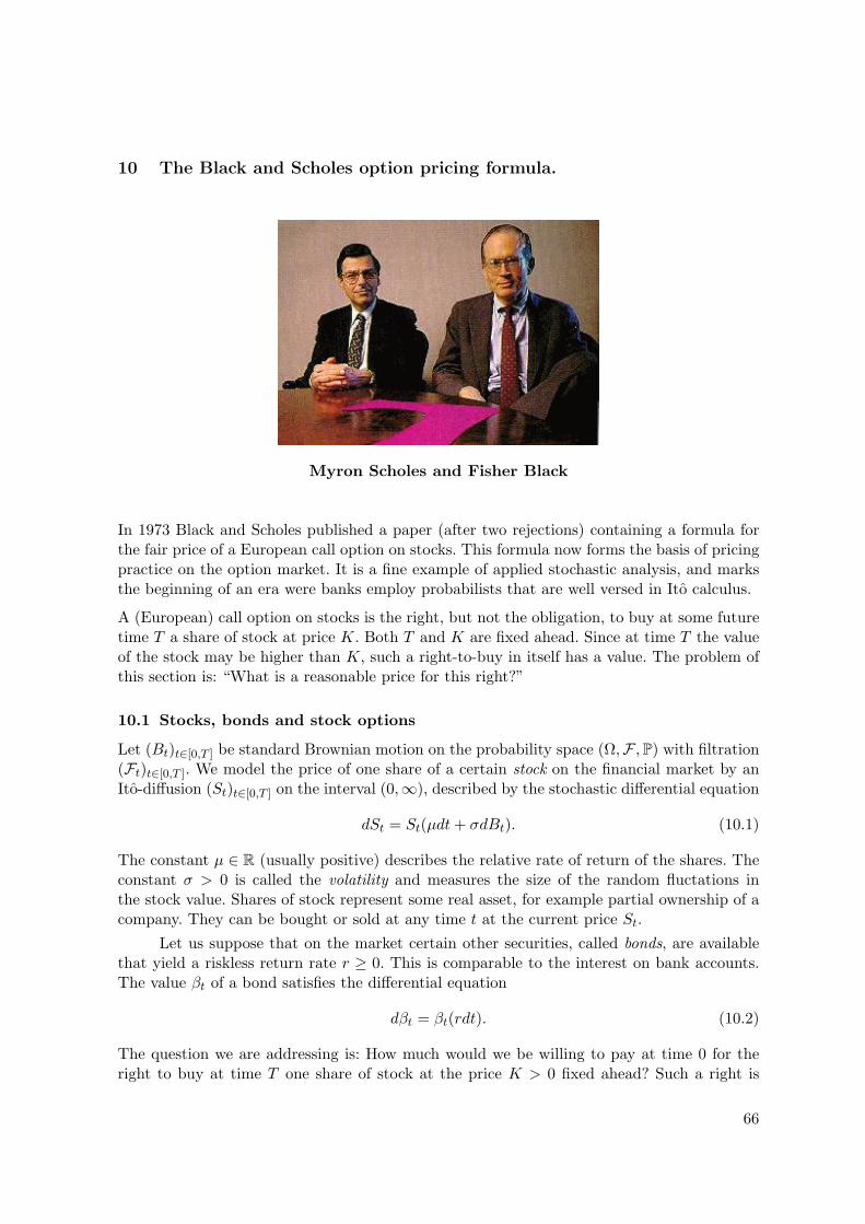
10 The Black and Scholes option pricing formula.

Myron Scholes and Fisher Black

In 1973 Black and Scholes published a paper (after two rejections) containing a formula forthe fair price of a European call option on stocks. This formula now forms the basis of pricingpractice on the option market. It is a fine example of applied stochastic analysis, and marksthe beginning of an era were banks employ probabilists that are well versed in Ito calculus.

A (European) call option on stocks is the right, but not the obligation, to buy at some futuretime T a share of stock at price K. Both T and K are fixed ahead. Since at time T the valueof the stock may be higher than K, such a right-to-buy in itself has a value. The problem ofthis section is: “What is a reasonable price for this right?”

10.1 Stocks, bonds and stock options

Let (Bt)t∈[0,T ] be standard Brownian motion on the probability space (Ω,F ,P) with filtration(Ft)t∈[0,T ]. We model the price of one share of a certain stock on the financial market by anIto-diffusion (St)t∈[0,T ] on the interval (0,∞), described by the stochastic differential equation

dSt = St(µdt+ σdBt). (10.1)

The constant µ ∈ R (usually positive) describes the relative rate of return of the shares. Theconstant σ > 0 is called the volatility and measures the size of the random fluctations inthe stock value. Shares of stock represent some real asset, for example partial ownership of acompany. They can be bought or sold at any time t at the current price St.

Let us suppose that on the market certain other securities, called bonds, are availablethat yield a riskless return rate r ≥ 0. This is comparable to the interest on bank accounts.The value βt of a bond satisfies the differential equation

dβt = βt(rdt). (10.2)

The question we are addressing is: How much would we be willing to pay at time 0 for theright to buy at time T one share of stock at the price K > 0 fixed ahead? Such a right is

66

called a European stock option. The time T is called the expiry time, the price K is called theexercise price. This option pricing problem turns out to be a problem of stochastic control.

Another type of option is the American stock option, where the time at which the sharescan be bought is not fixed beforehand but only has an upper limit. The pricing problem forAmerican stock options contains, apart from a stochastic control element, also a haltingproblem. It is therefore more difficult, and we leave it aside.

The solution to the European option pricing problem is given by the Black and Scholesoption pricing formula (10.4) appearing at the end of this Section. As this formula does notlook wholely transparant at first sight, we shall introduce the result in three steps, raising thelevel of complexity slowly by introducing the ingredients one by one.

10.2 The martingale case

Let us first suppose that both the stock price and the bond price are martingales: µ = r = 0in Equations (10.1) and (10.2). For bonds this simply means that their price is constant: theyare the stock-market equivalent of bank notes. For stocks it means that their price behaveslike the exponential martingale found in Chapter 5:

St = S0 exp

(σBt − 1

2σ2t

).

In this stationary world our option pricing problem is easy: a fair price q at time 0 of theright to buy at time T a share of stock at the price K is

q := E((ST −K)+

), (10.3)

where x+ stands for max(0, x). Indeed, if the stock value ST turns out to be larger than theexercise price K, then the holder of the option makes a profit of ST −K by buying the share ofstock at the price K that he is entitled to, and then immediately selling it again at its currentvalue ST . On the other hand, if ST ≤ K, then his option expires as a worthless contract.

Since we know the price process St to be an exponential martingale, we can explicitlyevaluate the option price q:

q = E((ST −K)+

)= E

((S0e

σBT− 12σ2T −K

)+)=

∫ ∞

−∞

(S0e

w− 12σ2T −K

)+φσ2T (w)dw

=

∫ ∞

log KS0

+ 12σ2T

(S0e

w− 12σ2T −K

)φσ2T (w)dw

= S0Φσ2T

(log

S0K

+1

2σ2T

)−K Φσ2T

(log

S0K

− 1

2σ2T

),

(10.4)

where Φλ : u 7→ 1√λΦ(

u√λ

)is the normal distribution fuction with mean 0 and variance λ,

and φλ = 1√2πλ

exp(−w2/2λ) is the associated density function. In (10.4) we have made use

of the equalities

ew− 12λφλ(w) = φλ(w − λ),

67

and ∫ ∞

xφλ(w)dw = Φλ(−x).

The above option pricing formula covers the case µ = r = 0. Surprisingly, it also coversthe case µ = 0, r = 0, i.e., µ plays no role in the final result. In fact, the full Black andScholes option pricing formula is obtained by substituting Ke−rT for K to take devaluationinto account. It was this surprising disappearance of µ from the formula that caused thedifficulties that Black and Scholes experienced in getting their result accepted.

And indeed, for a justification of these statements we need a considerable extension ofour theoretical background.

10.3 The effect of stock trading

If we now drop the assumption that µ = 0, but keep r = 0, the intuitive argument leadingto (10.3) breaks down. Indeed, if µ > 0, then there is an upward drift in the stock value thatmakes “dollars at time 0” inequivalent to “dollars at time T”. Simply building in a discountfactor e−µt is ill-founded, and will in fact turn out to be incorrect. We shall have to considerseriously the definition of a “fair price”. It is reasonable to base such a definition on thequestion what else could be done with a capital q during the interval of time [0, T ]. Thisbrings us to the subject of trading.

Suppose that a dealer in securities enters the market at time 0 with a capital q. He buysan amount a0 of stock at the current price S0, keeping the rest b0 := q − a0S0 in his pocketin the form of banknotes. Then at the times t1 < t2 < t3 < · · · < tn(= T ) he repeats thefollowing procedure. Let i ∈ 0, 1, 2, · · · , n−1. At time ti+1 our dealer, judging the past stockvalues St, (0 ≤ t ≤ ti+1), decides to change his amount of stock from ati to ati+1 by buying orselling. If he chooses to buy more than his capital can pay for, he borrows money, (thus makingbt+1 negative), and keeps in mind that his loan must be paid back in due course, say aftertime T . Nevertheless, his tradings must be self-financing, i.e., our dealer spends no money,and obtains no money from outside, other than the loans and stock tradings mentioned. Sohis total capital (“portfolio value”) just before ti+1 must be equal to the portfolio value justafter this moment of time:

atiSti+1 + bti = ati+1Sti+1 + bti+1 , (i = 0, 1, · · · , n− 1). (10.5)

Employing the notation of Chapter 2,

(∆t)i := ti+1 − ti; (∆X)i := Xti+1 −Xti ,

we may write (10.5) as(∆a)i(Sti + (∆S)i) + (∆b)i = 0. (10.6)

We note that this equation expresses a kind of “time delay”: the amount ati of stock boughtat time ti only has its effect at time ti+1. This delay will remain even after the continuoustime limit is taken, when it will give rise to an Ito-term.

Now consider the portfolio value Ct at time t:

Ct := atSt + bt.

68

We note that in the case of self-financing trade:

(∆C)i := Cti+1 − Cti

= ati+1Sti+1 + bti+1 − atiCti − bti

= (ati+1 − ati)(Sti+1 − Sti) + (bti+1 − bti) + (ati+1 − ati)Sti + ati(Sti+1 − Sti)

= (∆a)i(∆S)i + (∆b)i + (∆a)iSi + ai(∆S)i

Therefore (10.6) can be written concisely as

(∆C)i = ai(∆S)i.

Now, since there is no essential limit to the frequency of trade, the partition of [0, T ] generatedby the sequence of times 0 = t0 < t1 < t2 < · · · < tn−1 < tn = T can be made arbitrarily fine.It is therefore reasonable to make the following idealisation.

Definition. A self-financing trading strategy is a pair (a, b) of square-integrable adaptedprocesses on [0, T ] with continuous paths, such that the sum Ct := atSt + bt satisfies

dCt = atdSt. (10.7)

We are now in a position to define what we mean by the “fair price” of a claim oroption. Let g : [0,∞) → [0,∞) be measurable. By a claim to g(ST ) we mean the right to cashin at time T the amount g(ST ), which depends on the current stock value ST at time T .

Definition. A claim to g(ST ) is called redundant if there exists a self-financing strategy (a, b)such that with probability 1,

CT := aTST + bT = g(ST ).

By the fair price F(g(ST )) of a redundant claim to g(ST ) we mean

F(g(ST )) := C0 = a0S0 + b0.

So F(g(ST )) = q if q could be used as the starting capital q = a0S0 + b0 for a trading(a, b) that ends up with g(ST ) with certainty.

10.4 Motivation

In the financial literature the above definition is usually motivated by the following argument(a so-called arbitrage argument).

Suppose that claims to g(ST ) were traded at time 0 at a price p higher than q. Thenit would be possible to make an unbounded and riskless profit (an “arbitrage”) by selling nsuch claims for the market price p, then to reserve an amount nq as initial capital for theself-financing strategy (na, nb) — yielding with probability 1 the amount ng(ST ) needed tosatisfy the claims — and then to pocket the difference n(p−q). Conversely, if the market pricep of the claim would be lower than q, then one could buy n claims and apply the strategy(−na,−nb) yielding an immediate gain of n(q−p) at time 0. At time T one could cancel one’s

69

debts by executing the n claims to g(ST ). It should be admitted that this second strategy,involving negative share holdings (or short sales of stock), is somewhat more artificial thanthe first. But clearly, the possibility of arbitrage is not fair.

This concludes the motivation of Definition 10.3. In economic theory one often goesone step further and assumes that arbitrage in fact does not occur. It is claimed that thepossibility of arbitrage would immediately be used by one of the parties on the market, andthis would set the market price equal to the fair price.

10.5 Results

Theorem 10.1 Let g ∈ C0(0,∞). On a stock market without bonds or interest (i.e., withr = 0), the fair price at time 0 of a claim to g(ST ) at time T > 0 is

F(g(ST )) = E(g(XT )),

where (Xt)t∈[0,T ] is the exponential martingale with parameter σ starting at S0, i.e., thesolution of the stochastic differential equation

dXt = Xt(σdBt) with X0 = S0. (10.8)

Corollary 10.2 In the absence of bonds or interest the fair price at time 0 of an option toa share of stock at time T is

F((ST −K)+

)= E

((XT −K)+

),

whereXt is the exponential martingale of Theorem 10.1. The right hand side is given explicitlyby (10.4).

Proof. Approximate the function x 7→ (x − K)+ by a sequence gn ∈ C0(0,∞) ad applyTheorem 10.1. 2

We now give the proof of Theorem 10.1.

Proof. Let A := σ2x2 ∂2

∂x denote the generator of the diffusion Xt in (10.8), and define

ft := e(T−t)Ag, (t ∈ [0, T ]).

Define a trading strategy (a, b) by

at := f ′t(St) and bt := ft(St)− Stf′t(St).

Then aTST + bT = fT (ST ) = g(ST ). Moreover, (a, b) is self-financing since the total portfoliovalue Ct satisfies

dCt := dft(St)

=

(dftdt

)(St)dt+ f ′t(St)dSt +

12f

′′t (St)(dSt)

2

= −(Aft)(St)dt+ atdSt +12σ

2S2t f

′′t (St)dt

= atdSt.

70

It follows that the fair price at time 0 is given by

F(g(ST )) := a0S0 + b0 = f0(S0) =(eTAg

)(S0) = E

(g(XS0

T )).

2

Note that there is no µ in this proof! Apparently the fair price at time 0 is not influencedby µ To begin to understand this fact, we take the case g(x) = x. Clearly the fair price attime 0 of a share at time T is just S0, not E(ST ): St is automatically a “martingale under F”.

Explicit calculation of the strategy for the case g(x) = (x−K)+ of a stock option yields

at = Φσ2(T−t)

(log

StK

+ 12σ

2(T − t)

);

and

bt = −K Φσ2(T−t)

(log

StK

− 12σ

2(T − t)

).

These expressions describe a smooth steering mechanism, moving from the initial value (a0, b0)to the final value (aT , bT ), given by

(aT , bT ) =

(0, 0), if ST ≤ K;

(1,−K), if ST > K.

Thus the pair (at, bt) always moves inside [0, 1] × [−K, 0], the strategy always involves bor-rowing of money in order to buy up to one single share of stock. In cases where the option ischeap, relatively much has to be borrowed in order to imitate the workings of the option.

10.6 Inclusion of the interest rate

We complete our treatment of the Black and Scholes model by including bonds, securitiesthat yield a riskless return. The presence of these bonds on the market leads to a constantdevaluation. Therefore, measured in “dollars at time 0”, the exercise price of the option willonly measure Ke−rT . Interestingly, this is the only change (in the Black and Scholes) resultdue to a nonzero interest rate: if again Xt denotes the exponential martingale with parameterσ and S0 the stock value at time 0, then

F((ST −K)+

)= E

((XT −Ke−rT )+

).

This result will come out as a combined effect of an upward drift and a discount.

In the presence of bonds, a self-financing strategy is to be defined as a pair (a, b) ofadapted processes with continuous paths such that the total portfolio value Ct := atSt + btβtsatisfies

dCt = atdSt + btdβt.

Theorem 10.3 On a stock market with stocks and bonds the fair price at time 0 of a claimto g(ST ) at time T > 0 is

F(g(ST )) = e−rTE(g(YT )),

where (Yt)t∈[0,T ] is the solution of the stochastic differential equation

dYt = Yt(rdt+ σdBt) with Y0 = S0.

71

Proof. Let B := rx ∂∂x + σ2x2 ∂2

∂x2 be the generator of the diffusion Yt and define

ft := e(T−t)(B−r)g, (t ∈ [0, T ]).

Let the strategy (a, b) be given by

at := f ′t(St) and bt :=1

βt

(ft(St)− Stf

′t(St)

).

(Recall that βt = ert by (10.2).) Then aTST + bTβT = fT (ST ) = g(ST ). Moreover, (a, b) isself-financing since

dCt := dft(St)

= −(B − r)ft(St)dt+ f ′t(St)dSt +12f

′′t (St)(dSt)

2

=

(−(B − r)ft(St) +

12σ

2S2t f

′′t (St)

)dt+ f ′t(St)dSt

= r

(ft(St)− Stf

′t(St)

)dt+ f ′t(St)dSt

= btdβt + atdSt.

It follows that

F(g(ST )) := f0(S0) =(eT (B−r)g

)(S0) = E

(e−rT g(YT )

).

2

Corollary 10.4 The fair price of a stock option is

F((ST −K)+

)= e−rTE

((YT −K)+

)= E

((XT − e−rTK)+

)= S0Φ

(log

S0K

+ (r + 12σ

2)T

)−Ke−rTΦ

(log

S0K

+ (r − 12σ

2)T

).

Proof. The first equality is Theorem 10.3, the second equality follows from the fact thatYt = ertXt, while the third equality is (10.4). 2

72