Embed Size (px)
Citation preview
J Fluid Mech (1977) vol 82 part 4 p p 747-765
Printed in Great Britain 747
Stochastic closure for nonlinear Rossby waves
By GREG HOLLOWAYT AND MYRL C HENDERSHOTT
Scripps Institution of Oceanography La Jolla California 92037
(Received 7 January 1976 and in revised form 14 April 1977)
An extension of the turbulence lsquotest-field modelrsquo (Kraichnan 1971 a) is given for two- dimensional flow with Rossby-wave propagation Such a unified treatment of waves and turbulence is necessary for flows in which the relative strength of nonlinear terms depends upon the length scale considered We treat the geophysically interesting case in which long fast Rossby waves propagate substantially without interaction while short Rossby waves are thoroughly dominated by advection We recover the observations of Rhines (1975) that the tendency of two-dimensional flow to organize energy into larger scales of motion is inhibited by Rossby waves and that an initially isotropic flow develops anisotropy preferring zonal motion The anisotropy evolves to an equilibrium functional dependence on the isotropic part of the flow spectrum Theoretical results are found to be in quantitative agreement with numerical flow simulations
1 Introduction We consider statistically homogeneous non-divergent barotropic flow on a 8-
plane ie
where $ is the stream function and 6 = Vz is the vertical component of the vorticity The Jacobian term provides advection of vorticity while the p-term propagates Rossby waves Some form of dissipation is required in (1) but for the moment we avoid stating our prejudices on dissipation Now we impose that g be spatially periodic on a rectangular lsquocellrsquo and so be given by a discrete Fourier series
g = [ k ( t ) erdquordquo k
The Fourier transform of (1) is
where y = -3kxk2 Ak = k x pp2 and v k is included as an explicit but as yet unspecified dissipation function vk = d ( k ) Our aim will be a statistical description of (2) averaging in principle over many realizations of the flow to obtain the evolution from statistically prescribed initial conditions of ensemble-average covariances (ck 5-k)
t Present address National Center for Atmospheric Research Advanced Study Program PO Box 3000 Boulder Colorado 80307
available at httpswwwcambridgeorgcoreterms httpsdoiorg101017S0022112077000962Downloaded from httpswwwcambridgeorgcore Access paid by the UCSD Libraries on 08 Mar 2017 at 223436 subject to the Cambridge Core terms of use
748 G Holloway and M C Hendershott
If nonlinearity is sufficiently weak that a wave propagates over several wave periods without being significantly modified by interaction with other waves then neglecting dissipation we might proceed by a resonant wave interaction calculation (Kenyon 1964 Longuet-Higgins amp Gill 1967) One supposes amp(t) = +(r) exp ( -iwkt) where r = s2t is the slow time scale of wave interaction t is a fast time scale with units of the wave period and E is a small number proportional to the amplitude of the motion By integrating (2) over the fast time scale as t + 03 while supposing that E + 0 such that s2t remains finite one obtains contributions to the slow rate of change of from resonant wave triads satisfying
p + q = k
and u p + w~ = wk (3)
Such a result is obtained only asymptotically for E -+ 0 A problem is that the dispersion relation wk = -Pkzk2 provides very long periods for very short waves so that no matter how weak the flow (ie how long the interaction time) the very short waves will interact significantly in times short compared with their periods More trouble- some yet are the components of zonal flow with k = 0 and hence indefinite periods All interaction with the zonal flow is essentially strong regardless of its amplitude Thus for a continuous spectrum of Rossby waves we may not consider E to be small
If on the other hand we take P negligibly small then (2) is the equation of lsquotwo- dimensional turbulencersquo The significant feature of this flow is that vorticity is ad- vected without stretching in contrast with the tendency in three-dimensional flow to extend vortex lines Thus two-dimensional advection preserves both mean energy density B = sm and mean lsquoenstrophyrsquo density z = ldquo (Overbars denote area averages over the periodic flow cell) Now energy cannot cascade into ever finer scales since this would entail generation of enstrophy Instead one speaks of a cascade of enstrophy into finer scales together with an lsquoinverse cascadersquo of energy into larger scales of motion (Kraichnan 1967) A problem arises when we attempt to relax periodicity by letting the period length become arbitrarily large No matter how small 3 is we shall admit long waves with periods small compared with any interaction time In other words on an unbounded P-plane we may not consider E to be large
Rhines (1975) suggests that we think of wavenumber space as divided into a wave regime and a turbulence regime with a lsquosoftrsquo border between The border can be defined approximately by the condition that wave phase speeds equal fluid particle speeds In the turbulence regime enstrophy will cascade towards high wavenumbers while energy cascades towards low wavenumbers However the energy cascade will encounter this waves-turbulence border beyond which further energy transfer can proceed only weakly by resonant wave interaction The result is to accumulate energy near the waves-turbulence border Rhines then argues that by inhibiting energy trans- fer to low wavenumbers the flow becomes limited in its enstrophy transfer to high wavenumbers resulting in a high wavenumber spectrum which falls off more steeply than in a flow without Rossby waves Finally the anisotropic dispersion relation results in anisotropic evolution from an initially isotropic flow field Numerical simulations show a marked tendency to prefer zonal (east-west) motion Rhines suggests that this may be due to a stabilizing effect of P on zonal flow possibly even resulting in evolution towards a state of steady zonal jets
Numerical simulations provide qualitative support for Rhinesrsquo description The
available at httpswwwcambridgeorgcoreterms httpsdoiorg101017S0022112077000962Downloaded from httpswwwcambridgeorgcore Access paid by the UCSD Libraries on 08 Mar 2017 at 223436 subject to the Cambridge Core terms of use
Xtochustic closure for nonlinear Rossby wave8 749
energy spectrum does become peaked near a waves-turbulence border The high wavenumber spectrum does fall off more steeply with 8 present though as we shall see this may be a consequence of Rhinesrsquo assumption of viscous-type dissipation vk = vk2 Finally simulations do become anisotropic though an end state of steady zonal flow remains conjectural However this phenomenological admixture of turbu- lence and waves ideas does not admit quantitative calculation Also the description is essentially local in wavenumber space turbulence-like dynamics bring energy up to a border where somehow a transition to wave-like dynamics is effected Indirectly the suppression of energy transfer comes to be felt as a limitation on enstrophy transfer at high wavenumbers But are there non-local direct interactions of waves and turbu- lence Does anisotropy find an equilibrium state short of steady zonal flow
This paper attempts a more analytical treatment by extending a class of turbulence theories to include wave propagation The derivation does not depend upon non- linearity being either weak or strong In the limit where waves dominate nonlinearity we just recover a resonant wave interaction approximation
2 Markovian quasi-normal (MQN) closure We employ a closure in which evolution of second moments (Ck(t) ck(t)) is expressed
in terms of the values of the second moments (CD(t) CPD(t)) in other modes with all quantities known only at the instant t This requires that the statistics have evolved to a state of quasi-stationarity by which we mean that secondmoments change slowly during a response time of higher moments (the time in which an arbitrary small perturbation to any higher moment will decay)
The label lsquoquasi-normalrsquo here is a bit misleading Although a formal appeal is sometimes made to expansion about a normal distribution the resulting closure may describe statistics which are far from normally distributed The wave interaction approximation (Hasselmann 1962 Benney amp Saffman 1966) is a member of the MQN class as are a variety of turbulence models in particular the lsquo test-field modelrsquo (TFM) which has shown agreement with numerical simulations of turbulence (Kraichnan 1971a Herring et al 1974) The lsquodirect-interaction approximationrsquo (DIA) for turbulence (Kraichnan 1958 1959) is a more fundamental approach couched in simultaneous equations for evolution of mode response functions Gk(t t lsquo ) and time-displaced covariances (Ck(t) C J t rsquo ) ) However the stationary DIA may be abridged to an MQN form by assuming ad hoc that time-displaced covarianees decay exponentially as ( C k ( t ) C-k(trsquo)) = (Ck(t) C - k ( t ) ) exp ( - T k l t - - t rsquo l ) for some qr Relationships among the various MQN turbulence models and their relation to the DIA are reviewed by Leslie (1973 chaps 7 and 11) and by Orszag (1974)
Different approaches may be employed in deriving or justifying a closure model Here we give a heuristic sketch which differs somewhat in style from other accounts eg Orszag (1974) but is equivalent in its consequences
Ensemble averaging (2) and deleting for the moment all subscripts coefficients and summations we have an unclosed set of equations
(4a) (4b) ( 4 4
d(CC)Idt = (CO + (CCC) d(CCOldt = (CCC) + ( 5 0 KO + (CcCC)c
dltCCCOCldt = ltCCCC)C + ltCC) ( C m + accY
available at httpswwwcambridgeorgcoreterms httpsdoiorg101017S0022112077000962Downloaded from httpswwwcambridgeorgcore Access paid by the UCSD Libraries on 08 Mar 2017 at 223436 subject to the Cambridge Core terms of use
750 G Holloway and M C Hendershott
etc A superscript C denotes a cumulant ie the remainder of a moment say of the fourth moment (ccco after any contributions from non-vanishing lower moments (here products of second moments (flo (co) have been removed Terms appear on the right sides of ( 4 ) owing to the linear and nonlinear terms in (2) In each of (4u-c) nonlinearity introduces the next higher cumulant hence the closure problem
What is appropriately termed a lsquo quasi-normal rsquo or fourth-cumulant discard hypo- thesis closes ( 4 ) by taking (campQc = 0 for all time However direct integration of (4a b ) then produces quite unrealistic results for turbulence evidenced in part by unrealiz- able negative values for ( ampI2) (Ogura 1962) The wave interaction approximation is different based on distinction of fast and slow time scales t and T integration of ( 4 b ) is considered only in the limit of large t and leads without dissipation to indefinitely large values of (cco on a vanishingly small (in continuous wavenumber space measure) resonant interaction set (3) Substitution of these resonant members of (4b) into ( 4 a ) gives the wave interaction approximation and assures that 0 Given plausible initial conditions the evolution of (cccoc turns out not to matter in the limit of vanishingly weak nonlinearity On the other hand Ogurarsquos calculations clearly indicate the significant role of fourth cumulants in turbulence
A plausible turbulence model without waves is obtained by observing that in ( 4 b ) products (co (go cause (cco to build up until checked at some level by a dissi- pation term - v(LJJJ obtained from (2) If dissipation is weak (cco will become quite large unless it is being relaxed statistically by (cccoc which we therefore assume to be simply of the form ([[cot = - p ( [ c o where p is some coefficient Observe that u is not a usual eddy viscosity since we have not altered (4a) Now by quasi-stationarity we integrate ( 4 b ) over a time large compared with (v +u)-l and substitute the result into ( 4 a ) to get
with 8 = (v +u)-l The object of an MQN turbulence theory is to evaluatep or equiva- lently 8 The TFM is one such evaluation The wave interaction approximation uses 8 to isolate resonant wave triads 8 = n6(wp +up - wk) with 6 the Dirac delta-function
3 lsquoTest-field modelrsquo with waves
to model the evolution of second moments Iz(t) = (ck(t) c-k(t)) by an equation Restoring the algebraic detail which wad deleted in the preceding section we seek
where
and
are geometric coefficients obtained from ( 2 ) a k p g and bkp depend only on the lengths k p and q Sums over wave vectors k p or q range over some finite set of modes usually defined by requiring that the wave vectorrsquos length be less than some k It is this Fourier truncation of (1) in passing to (2) which has caused us to admit the explicit dissipation vk However the form of vk still need not concern us
available at httpswwwcambridgeorgcoreterms httpsdoiorg101017S0022112077000962Downloaded from httpswwwcambridgeorgcore Access paid by the UCSD Libraries on 08 Mar 2017 at 223436 subject to the Cambridge Core terms of use
Stochastic closure for nonlinear Rossby waves 751
e is the unknown array which becomes the focus of our attention If O-k9q is constrained to be invariant to permutations of its indices then the sum of the right- hand side of ( 5 ) over k vanishes Likewise the weighted sum of Ilk2 times the right-hand side of ( 5 ) vanishes Thus the constraint to a fully symmetric O-k9 assures that non- linear interaction preserves both mean enstrophy and mean energy density
The lsquotest-field modelrsquo (Kraichnan 1971 a ) completes the specification of O-k9q up to a single universal empirical constant which could be evaluated for example in terms of an estimated Kolmogorov inertial range constant We sketch the TFM here appealing to a correspondence between ( 5 ) and stochastic models of Langevin type (Leith 1971)
For the moment we omit waves considering just two-dimensional turbulence Equation ( 5 ) attempts to approximate the statistical evolution of (2) But (5) is also an exact closure for a set of linear stochastic differential equations
where
and ( fk( t ) f -k( t lsquo ) ) = ( e-k9pakpqz92g) s(t- t rsquo ) -
Equation (6) is a Langevin equation describing a random variable [k evolving under the influence of a linear drag vk + Tk and a random force fk
Physically O-k9q has the role of a relaxation time of phase correlations among modes k p and q which we might estimate by some heuristic argument However the correspondence between (5) and (6) holds for any non-negative choice of O-kBq As a linear equation (6) is characterized by its Greenrsquos function Gk(t t rsquo ) Thus with- out using further physical arguments we may already obtain a form for O-k9q in terms of the form of (6) This integral time scale for correlations among the stochastic model variables c-k amp and ta is
9+a=k
G-k(t trsquo) G9(t t rsquo ) Gq(t trsquo) dtrsquo - - m
O-k9a = J (7)
Equations (5)-(7) are a closure for (2) omitting waves Unfortunately a spurious effect has been introduced which becomes evident in the stochastic model representa- tion (6) Evolution of each stochastic variable [k depends only on the variance in other modes (c [-J while any phase information is lost Very large scales of motion approaching uniform translation contribute to amp and hence to a rapid decrease of q t t rsquo ) in t - trsquo in turn resulting in a small value for O-k9a In reality large-scale motion advects triple phase correlations nearly coherently and so in the limit of uniform translation ought to have no effect on the value of O-k9q
The TFM restoresha proper Galilean invariance by adopting O-k9q in the form (7) while estimating a modified k( t t rsquo ) which suppresses the effect of large-scale advection The heuristic argument (Kraichnan 1971 a) is that O-k9 represents the deformation of fluid parcels In a Lagrangian description of the motion deformation is accomplished only by pressure and viscous forces Accordingly we seek that part 6 of the overall Gk which is due to pressure effects Pressure in incompressible Navier-Stokes flow is evaluated from the incompressibility condition ie pressure is the agent which pre- vents a eolenoidal flow field from developing a longitudinal part Thus a measure of
available at httpswwwcambridgeorgcoreterms httpsdoiorg101017S0022112077000962Downloaded from httpswwwcambridgeorgcore Access paid by the UCSD Libraries on 08 Mar 2017 at 223436 subject to the Cambridge Core terms of use
752 G Holloway and M C Hendershott
the pressure effect is had by computing the rate at which a solenoidal flow would generate a longitudinal flow in the absence of a pressure term This measure of the pressure effect is asswned to be related to the actual triple-moment relaxation through an empirical constant of proportionality
Kraichnans derivation of the TFM for Navier-Stokes turbulence is given in velocity- component notation which is inconvenient for many problems of quasi-geostrophic motion eg Rossby waves We therefore rederive the TFM for two-dimensional turbulence in the scalar notation of stream functions and velocity potentials Consider an advecting field given by a vorticity fl having the statistics of the turbulence Let this field advect a passive test field given by a stream function $ and velocity potential 4 x = V2$ and u = Vz4 are the vorticity and divergence of the test field We seek the rate a t which advection by y will mix the two parts x and u This is
and
for which an MQN closure is
A
where x k = ( x k x - k ) amp = ( u k u - k ) and where e-k9q is another unknown array We observe that these equations describe the solution of another Langevin model
(ddt + f i k ) ek = fk
where f i k = x -k pq skpp 2 9 P+q=k
with ampkp = I k X pI4k2p4q2 The argument is that the rate fik is a measure of the rate uk of self-deformation of the 5 field Including viscosity p k is written as
where g is a phenomenological constant of order unity and e-k9q is again given by (7) but with a modified Greens function 4 ( t t) depending on uk in place of q k
Now the reintroduction of waves is straightforward Since wave propagation results in deformation of fluid parcels this linear effect enters the modified Greens
0 for t lt t 8(t - t ) for t 2 t
function as (ddt + i u k +A) d k ( t t ) =
available at httpswwwcambridgeorgcoreterms httpsdoiorg101017S0022112077000962Downloaded from httpswwwcambridgeorgcore Access paid by the UCSD Libraries on 08 Mar 2017 at 223436 subject to the Cambridge Core terms of use
Stochastic closure for nonlinear Rossby waves 753
We are therefore obliged to consider complex ik(ttrsquo) and hence by (7) complex 1 9 - ~ ~ ~ However in closing (2)-(5) one adds complex conjugates thus retaining only the real part of (7) In its quasi-stationary form 8-kvq is
aamp t rsquo ) av(t t rsquo ) a($ trsquo) dtrsquo
4 Comparison with numerical experiment We have integrated ( 2 ) over a set of wave vectors lying in an annulus between
1 k( = 1 and I k( = k = 62 The amplitude of the motion is scaled such that a nominal lsquoeddy turnover timersquo 27rf M 1 where is the root-mean-square vorticity It is observed that a unit of time corresponds to significant evolution of the flow Integrations are then carried to t = 64 well into the quasi-stationary decay of the flow Initial conditions consist of a random phase c k in an isotropic wavenumber band near k = 1 1 As the flow evolves and energy migrates into larger scales the character- istic energetic wavenumber k decreases to k M 5 at t = 64
The relative role of p can be expressed by defining k ) = [rm a wavenumber for which the Rossby-wave period of the faster westward-propagating waves ( M 27rklp) is of the order of the eddy turnover time However we caution against too literal an interpretation of k) as a waves-turbulence border Rather k ) is the lower wavenumber of a transitional region roughly from k) to perhaps 3kb within which most triad interactions are characterized by M wkv a where p and q are typically greater than k for which we find below that p M CrJ27r We have investigated three choices of p 3 = 0 ( k ) = 0 ) p = 125 ( k ) = 15 +- 25) and 3 = 25 ( k ) = 3 +- 5 ) where we indicate in parentheses that kl increases as [rem8 decays from an initial value crmfl M 8 toafinalvalue Cr x 5The casesmaybedescribedas lsquonoprsquo(forreference) lsquosmall prsquo and lsquomoderate prsquo We have not investigated the case of large 6 in part be- cause we intend shortly to approximate ( 5 ) in an expansion about isotropy ie about p = 0 and in part because the extension of resonant interaction theories to waves of small but finite amplitude warrants a more careful study on its own
Lastly we must provide a truncation-induced dissipation vk At present there appears to be no fundamental justification for the form of the dissipation operator We have chosen
vokamp x O for k lt kd vk = (k - k)2 ( k 2 - k2)2 for k 2 k
a form which is discussed though hardly justified by Holloway (1976) With k = 62 we have taken k = 45 and vo = 0005 a conservatively large damping rate which results in a falling off of the spectrum in the dissipation range k lt k lt k
In turbulence theory it is usually most convenient to assume isotropic statistics summing the modal z k in concentric shells to obtain a scalar enstrophy spectrum Z(k) Then ( 5 ) gives the evolution of Z ( k ) in terms of integrals over Z ( k ) With I present we
available at httpswwwcambridgeorgcoreterms httpsdoiorg101017S0022112077000962Downloaded from httpswwwcambridgeorgcore Access paid by the UCSD Libraries on 08 Mar 2017 at 223436 subject to the Cambridge Core terms of use
754 G Holloway and M C Hendershtt
cannot assume isotropy Rather we follow Herring (1975) resolving Fourier harmonics
into angular
amp = Z(k) e i n h n
where $k is the angle between k and the kx axis Odd harmonics $amp 3$k etc vanish since 2 = 2-k The result is an open set of coupled nonlinear integral equations for the even harmonics Z(k) It is difficult to see how consistently to truncate this set both in the number of harmonics and in the order of coupling except for truncation at the lowest order in the departure from isotropy Thus we limit the representation to
2nkamp = Z ( k ) (1 - R ( k ) COS 2$k) (10)
where a term in sin 2k vanishes by symmetry about the kx axis In the appendix we substitute (10) into ( 5 ) integrating over $k and linearizing in the departure from iso- tropy ie at order R ( k ) or a t order p2 the lowest order in p The result is the following pair of equations for the isotropic enstrophy spectrum 2 ( k ) and the anisotropy R ( k )
d - R(k) = X( k ) +jkmsdpR( k p ) R(p) - v(k) R( k) dt 1
where
and
The various symbols are defined in the appendix Equation ( 11) describes the evolution of the isotropic enstrophy spectrum in terms of a forcing rate ( ( k ) and a damping rate q(k) Anisotropy does not appear in (1 1) However penters the coefficient Il(e) namely
Il(s) = 4ne(e2 + 2 4 4 where e(k p q) = (2k2pa) ( p ( k p q))
when k lt p q Equation (12) describes the evolution of the anisotropy in terms of a source term S ( k ) a transfer-of-anisotropy term with kernel K ( k p ) and a return-to- isotropy coefficient v(k) X(k) K ( k p ) and v (k ) are given by integrals over the isotropic spectrum with l3 entering the coefficients I I and 13
Figure 1 shows the isotropic enstrophy spectra at t = 64 in the three numerical experiments p = 0 p = 12-5 and p = 25 Also shown are calculated values of the TFM distortion rate p ( k ) according to equation (A 5) for the particular choice g = 07 of the TFM parameter Subsequently we shall investigate other choices g = 06 and
available at httpswwwcambridgeorgcoreterms httpsdoiorg101017S0022112077000962Downloaded from httpswwwcambridgeorgcore Access paid by the UCSD Libraries on 08 Mar 2017 at 223436 subject to the Cambridge Core terms of use
Stochastic closure for nonlinear Rossby waves 755
10
1 00
Y 10-1 N
10-2
1 0 - 3
I I
kd k FIGURE 1 (a) Observed isotropic enstrophy spectra at t = 64 B = 0 - - - B = 125 - l = 25 ( b ) Theoretical deformation rates p ( k ) calculated from the observed enstrophy spectra g = 07
100
lo-
Y a
10-2
1 0 - 3
g = 10 to be compared with a previous estimate g = 065 (Herring et al 1974) obtained in a direct simulation of two-dimensional turbulence Two immediate observations are that with 3 present less enstrophy is found in lower wavenumbers and that the high wavenumber spectra (k gt 10) are quite similar in the three experiments falling roughly along a power law with slope between k-1 and k2 Z ( k ) cc k-l would corres- pond to a Kolmogorov-type enstrophy-cascading subrange Over 10 lt k lt kd the theoretical u(k) is rather flat with a value of the order of cr m8 2~ x 1 supporting our earlier definition kb = 4[
To isolate the role of 4 we consider in figure 2 just the experiment with p = 125 In figure 2 (a) we reproduce the distortion rate p ( k ) along with the forcing rate [(k) and damping rate q(k) t(k) gt ~ ( k ) at very low and at very high wavenumbers indicates the transfer of enstrophy into these wavenumbers while [(k) lt q(k) near k x k x 5 indicates removal of energy from these wavenumbers [(k) and q(k) very nearly cancel over 10 -= k lt k In figure 2 ( b ) we recompute each of these rates for the same iso- tropic enstrophy spectrum but now omitting 4 The result is that all rates increase at all wavenumbers However the effect on spectral evolution is most evident for small wavenumbers k 5 kp where the difference [(k) -q(k) approximately triples in value Over 10 lt k lt k both [(k) and q(k) have increased but remain nearly in cancellation Finally and at first surprisingly [(k) - q(k) increases significantly in
available at httpswwwcambridgeorgcoreterms httpsdoiorg101017S0022112077000962Downloaded from httpswwwcambridgeorgcore Access paid by the UCSD Libraries on 08 Mar 2017 at 223436 subject to the Cambridge Core terms of use
756 Q Holloway and M C Hendersbtt 103
1 oz
10 h
Y u
h
100 P
h
Y x
lo-
4 1
kg = 27 kd k
D
FIGURE 2 (a) For the case p = 125 theoretical curves show the deformation rate p(amp) the damping rate ~ ( k ) and the forcing rate ampk) (a) The role of 8 in (a) is revealed by recomputing a) q(k) and [(k) with p set to zero
available at httpswwwcambridgeorgcoreterms httpsdoiorg101017S0022112077000962Downloaded from httpswwwcambridgeorgcore Access paid by the UCSD Libraries on 08 Mar 2017 at 223436 subject to the Cambridge Core terms of use
8 t o c h t i c closatce fix nonlinear Rossby waves 757
s a e c v) - 4
= 25
= 1
50 60 I Iii h 0 6 b30 40
25
FIGURE 3 Observed anisotropy at t = 64 for B = 0 P = 12-5 and P = 25
the dissipation range k gt kd though Rossby-wave propagation is totally negligible on these scales We return to the discussion of these results in the next section
Figure 3 shows the anisotropy in the three experiments at t = 84 With p present strong zonal ( R ( k ) gt 0) anisotropy develops in k 5 k j Although the zonal tendency is less near k the anisotropy increases slightly with k over k gt k When the flow has become quasi-stationary we expect a balance among the source transfer and return terms on the right-hand side of (12) Thus an equilibrium anisotropy profile is
This R(k) is shown in figure 4 for p = 125 and various choices of the TFM parameter g Good agreement is found near g = 0-65 Also shown are the contributions due to S(k)w(k) and I K ( k p ) R ( p ) d p v ( k ) in the case g = 07 Poorer agreement is found in figure 5 where p = 25 but this is to be expected since both the low-order representation (10) and the linearizing approximations made in obtaining (12) will fail as R(k) becomes a substantial fraction of upity For larger values of I one must return to the use of (6) (8) and (9) directly
available at httpswwwcambridgeorgcoreterms httpsdoiorg101017S0022112077000962Downloaded from httpswwwcambridgeorgcore Access paid by the UCSD Libraries on 08 Mar 2017 at 223436 subject to the Cambridge Core terms of use
768 a Holloway and M C Hendershott
I I SK ( k P) R ) d~
v ( k ) I
- 1 J
FIGURE 4 For the case B = 125 theoretical curves for the equilibrium anisotropy are compared with the observed anisotropy for three choices of the TFM parameter g Dashed curves show the roles of generation S(k) and transfer K ( k p) of anisotropy compared with a return-to-isotropy coefficient Hk)
5 Discussion A principal feature of this paper is that we avoid any fundamental distinction
between wave-like and turbulent dynamics The result provides a continuous des- cription ranging from waves of arbitrarily small amplitude to fully developed turbu- lence as given by (8) and (9) namely
8-kpq = ~kb(1(amppq+W2_tpq)
For vanishingly small amplitudes and omitting dissipation becomes vanishingly small while 8-kpq isolates resonant wave triads
8-kpq Td(0-k + u p + Oq) as PG2w2 0
The appearance of a transition from turbulence-like to wave-like dynamics may seem to occur abruptly since Pk the measure of nonlinearity increasingly draws its contn- butions only from nearly resonant wave triads In the limit of weak wave interaction dependence on the phenomenological constant g vanishes as one expects
available at httpswwwcambridgeorgcoreterms httpsdoiorg101017S0022112077000962Downloaded from httpswwwcambridgeorgcore Access paid by the UCSD Libraries on 08 Mar 2017 at 223436 subject to the Cambridge Core terms of use
Stochastic closure for nonlinear Rossby waves 759
I I S ( k ) 1 1 -
1
- -Y a j Q O 2 B
2
-4 I1
FIGURE 5 For the case 3 = 25 the theoretical equilibrium anisotropy is compared with the observed anisotropy Here the approximations made in obtaining (12) begin to fail 88 R a I
When advection thoroughly dominates wave propagation
and we recover the lsquo test-field model rsquo for two-dimensional turbulence The fact that this is the TFM is non-essential We could have introduced waves a t (7) obtaining the same wave interaction limit but a less accurate turbulence limit
We have examined the consequences of this closure for the case of barotropic Rossby waves for which U = -3kzk2 A wavenumber kb = bcrms where crm8 is the root-mean-square vorticity may be thought of as a lower wavenumber in a transitional zone roughly from kb to 3kb over which the character of the flow changes from more wave-like when k lt kb to more turbulence-like when k gt 3kb But neither regime is pure If kb is small compared with a characteristic energetic wavenumber k then any departure from isotropic statistics will be expected to be small and we can simplify the theory by considering the flow field to consist of an isotropic part plus a lowest wave vector harmonic of anisotropy The resulting approximations (1 1)
available at httpswwwcambridgeorgcoreterms httpsdoiorg101017S0022112077000962Downloaded from httpswwwcambridgeorgcore Access paid by the UCSD Libraries on 08 Mar 2017 at 223436 subject to the Cambridge Core terms of use
760 G Holloway and M C Hendershott
and (12 ) are found to be in some agreement with numerical simulations and to recover in part the observations of Rhines (1975)
One effect of $ is to suppress isotropic enstrophy or energy transfer into large scales of motion k lt k This effect is represented in the coefficient I in (11) For k 9 k I 3 477 as in turbulence whereas for k lt k I vanishes as I cc k In a subrange k lt k lt k lt k the effect of 3 is slight Asymptotically as kdlkl + a one may expect approach to an enstrophy-cascade subrange Z ( k ) K k-I Kraichnan (1971 b ) argues though that in a subrange as steep as k-l enstrophy transfer across very high wavenumbers is directly influenced by shearing on larger scales up to k leading to a logarithmic correction Z ( k ) K k-l (In kk)-- Now if k x k wave propagation renders the large scales less effective in shearing the fine scales sup- pressing somewhat the logarithmic correction Although numerical simulations with klk x 10 cannot realize such subranges we may observe in figure 1 that the spectra with $ present do exhibit flatter shapes over 10 lt k lt k implying that 3 is in- hibiting some enstrophy transfer across high wavenumbers This is supported by com- paring theoretical rates in figures 2 (a) and ( b ) which show that for a given isotropic spectrum 5 suppresses transfer into the dissipation range k gt k We infer that Rhinesrsquo observation that $ produces a steeper high wavenumber spectrum can be attributed to his use of a molecular form for the eddy viscosity ie vk = vk2 leading to a much broader dissipation range over which a steeper spectrum is expected
Another important effect of $ is to induce anisotropy For sufficiently small depar- tures from isotropy this effect is described by (12) in terms of a source or forcing term X(k) a transfer term I K ( k p ) R ( p ) dp by which anisotropy in the wavenumber p induces anisotropy in the wavenumber k and a relaxation or return-to-isotropy term v ( k ) R ( k ) When these three effects are balanced an equilibrium profile results as shown in figures 4 and 5 Dashed curves in these figures show the separate roles of the source term S ( k ) and transfer term I K ( k p ) R(p) dp scaled by v ( k ) for the choice g = 0-7 In fact $ acts as a source of anisotropy across the entire spectrum However v ( k ) x 2c(k) increases rapidly with k approximately as k2 as seen in figure 2 Thus the direct effect of $ results in large departures from isotropy in k lt kfl with negligible anisotropy over k gt k
Transfer of anisotropy alters this in three ways First small scales of motion are directly sheared by the large scales producing substantial zonal anisotropy in high wavenumbers despite the return tendency Second actual relaxation of anisotropy is not measured only by the return-to-isotropy coefficient v ( k ) For k M p gt k the positive kernel K ( k p ) tends to maintain anisotropy so that a continuous spectrum of anisotropy exhibits a weaker return tendency than one would suppose from v (k ) alone A third effect is due to negative K ( k p ) in k lt p x k Indeed it is a distinguish- ing feature of flow in two dimensions that the back-reaction from anisotropy in higher wavenumbers is to induce oppositely signed anisotropy (here meridional) in low wave- numbers As the figures show this meridional tendency acts effectively to limit the growth of zonal anisotropy in k lt k
A few further comments should be made Our use of the Rossby-wave dispersion relation was really incidental wk may be chosen arbitrarily so long as w-k = -wk suggesting that the formalism provides a more general closure for nonlinear waves An objection may be that Rossby waves are unusual since they derive from a first-
available at httpswwwcambridgeorgcoreterms httpsdoiorg101017S0022112077000962Downloaded from httpswwwcambridgeorgcore Access paid by the UCSD Libraries on 08 Mar 2017 at 223436 subject to the Cambridge Core terms of use
Stochastic closure for nonlinear Rossby waves 76 1
order wave equation ie allow only westward phase propagation More commonly we should encounter a second-order wave equation
However this factorizes into a pair of first-order equations in the variables
and
whence $k = (iak) (4g - i) closure consists of coupled master equations for three species of second moments ($i $Ik) (4 $k) and Re ($$ $f) These master equa- tions in turn correspond to components in the closure of a Langevin equation for a vector random variable (amp 4)
Another point is that if we strictly omit dissipation vk in the truncated set of equations (2) then methods of classical statistical mechanics may be applied to predict evolution to an inviscid equilibrium state
which is Kraichnanrsquos (1 967) equipartition solution for inviscid spectrally truncated two-dimensional turbulence It may be verified that this is the stable stationary solution of ( 5 ) omitting dissipation y1 and yz are determined from the average energy and enstrophy density and the truncation wavenumber We note especially that the inviscid equilibrium solution is independent of p so that the effects of 3 can be asso- ciated only with disequilibrium processes ie the response to the disequilibrium initial state and the role of dissipation Thus for example omitting dissipation in (2) we should expect much the same early departure from isotropy but after some very long time a complete return to isotropy Indeed substitution of the equilibrium isotropic spectrum Z ( k ) = 2nk( y1 + y2 k2) into (12) leads to R(k) = 0
One can imagine extending closure theories to include such effects as underlying irregular topography or the resolution of vertical degrees of freedom (baroclinic modes) Beginnings of such theories may be found in Herring (1977) Holloway (1977) and Salmon (1977) For the case of unforced inviscid spectrally truncated equations of flow in two layers with p irregular bottom topography and lateral boundaries absolute-equilibrium solutions are given by Salmon Holloway amp Hendershott (1976) A rather surprising feature of these absolute-equilibrium solutions is their physically realistic appearance despite quite unrealistic dynamics ie no average energy transfer among modes Equilbrium calculations show for example the prevalence of steady anticyclonic circulation around hills and the prevalence in two-layer flow of baro- tropic motion on scales larger than the internal Rossby radius of deformation The fact that such features persist qualitatively in realistic flows ie far from equilibrium indicates the statistical-mechanical tendency towards entropy maximization Com- pared with these equilibrium calculations turbulence theoretical closures can be characterized as theories of the disequilibrium statistical mechanics of quasi-geo- strophic motions as in the present case for Rossby waves
Though the results of closures for more complicated situations are not yet available we may still note some of the more immediate connexions with the present work
available at httpswwwcambridgeorgcoreterms httpsdoiorg101017S0022112077000962Downloaded from httpswwwcambridgeorgcore Access paid by the UCSD Libraries on 08 Mar 2017 at 223436 subject to the Cambridge Core terms of use
762 G Holloway and M C Hendershott
Thus in barotropic flow p is equivalent to a uniform bottom slope The tendency towards zonal anisotropy on the P-plane can be identified as a tendency towards flow along contours off IH where f is the rotation rate and H the depth of fluid However for topographic elements of finite extent an important difference arises on the un- bounded P-plane anisotropy is due solely to disequilibrium processes Over topography these disequilibrium processes enhancing contour flow of arbitrary sign act in the presence of an equilibrium tendency towards contour flow of a definite sign ie anti- cyclonic around hills Another effect of topography is to prevent the transfer of an- isotropy from the large to fine scales of motion plausibly by providing a negative contribution to the transfer kernel K ( k p ) and so producing a strong isotropizing effect on small scales In saying this we assume no mean zonal flow hence no resonant forcing of topographic Rossby waves Finally if we consider flow in two layers the effect of p is to propagate both faster barotropic and slower baroclinic Rossby waves It was noted that absolute equilibrium is characterized by barotropic motion on large scales with uncorrelated (mixed barotropic and baroclinic) motion on small scales Extension of the present barotropic theory then suggests that disequilibrium flow in two layers will develop an anisotropic correlation between say the stream functions in the two layers For flow initially isotropic and uncorrelated between layers we expect zonal flow on scales larger than the internal deformation radius to become well correlated (barotropic) while the larger-scale meridional flow remains uncorrelated (mixed barotropic and baroclinic) These concluding remarks are only qualitative In quantitative predictions and comparisons we can expect to assess both the validity of Markovian quasi-normal kinds of closures as well as their usefulness in realistic geophysical fluid dynamics
This study was prompted by the previous investigations of Dr P B Rhines Much of this development was substantially clarified in conversations with Dr J R Herring and Dr U Frisch Computations were performed at the National Center for Atmos- pheric Research which is sponsored by the National Science Foundation This work was supported under Grant NSF-ID074-23117
Appendix Low-order representation of anisotropy We have supposed that for sufficiently small B in the sense that kb is small compared
with k a departure from isotropy will remain small so that we may adopt a low- order representation
where Ak = 1 is the discrete wave-vector separation The consistency of (A 1) depends upon a calculation showing that R(k) is in fact small compared with unity We sub- stitute (A 1) into ( 5 ) and (8) approximating summation over p by integration
Subsequently we separate Z ( k ) and R(k) by integration
jd$
available at httpswwwcambridgeorgcoreterms httpsdoiorg101017S0022112077000962Downloaded from httpswwwcambridgeorgcore Access paid by the UCSD Libraries on 08 Mar 2017 at 223436 subject to the Cambridge Core terms of use
Stochastic closure for nonlinear Rossby waves 763
T
P
q = k m i n 4 q = k m a x
FIQURE 6 The domain of integration A
First it is convenient to change the integrals around a bit Let x y and z be the interior angles of a triangle opposite sides k p and q Integration is rewritten as
where the domain of integration A in which k p and q can form the sides of a triangle is shown in figure 6 Integration over A is considered to be performed twice once for each of the following choices of triad
p = kkz a = k 7 y (A 2)
In isotropic turbulence these choices do not matter and a single integration over A may be doubled
Equations (5) and (8) become
and
The separation of (A 3) into isotropic and anisotropic parts remains complicated by the (bk dependence of B-kpa which is due primarily to the k dependence of ampQq
The k dependence o f p k is weaker being derived from t3-kpa and R ) in (A4)
available at httpswwwcambridgeorgcoreterms httpsdoiorg101017S0022112077000962Downloaded from httpswwwcambridgeorgcore Access paid by the UCSD Libraries on 08 Mar 2017 at 223436 subject to the Cambridge Core terms of use
7 64 a Holloway and M C Hendershott
Thus on substitution from (A 4) into (A 3) we may consistently retain only an iso- tropic estimate of p k ie
Finally the smallness of kb compared with kl means that triads all of whose com- ponents lie in k 5 k will be relatively ineffective and we shall approximate the y5k dependence of d k 9 q by the k dependence in that mode k p or q which has the least modulus k p or q Call this mode 1 Then we take for O
Pu(amp +PufP) +lufa) --k93q = (p(k) + p ( p ) +p(q))2+ (32212) (1 + cos 2f$kcos 2a sin sin 2a)
where a is the interior angle opposite 1 when 1 + k and a = 0 when 1 = k Since this o-k p q remains symmetric in its indices we retain the property that nonlinear inter- actions preserve energy and enstrophy
Integrations over k are of three kinds
cos u d u 1 + (1 + cos u cos 201 f sin CT sin 2a)e
(2e2 + 4e + 1) COB 4a + 1 = 2ne
where e (k p q ) = (p(k)+p(p)+p(q))2( 322Z2) and the integral is the sum over the sign choices f With these expressions (A 3) yields (11) and (12) where terms of order R2 or order P2R are dropped Further discussion and interpretation of this derivation including calculation up to order P2R are given by Holloway (1976)
REFERENCES
BENNEY D J amp SAFFMAN P G 1966 Proc Roy SOC A 289 301 HASSELMANN K 1962 J Fluid Mech 12 481
HERXINO J R 1977 Two-dimensional topographic turbulence Submitted to J Atrnos Sci HERRING J R ORSZAG S A KRAICHNAN R H amp Fox D G 1974 J Fluid Mech 66 417 HOLLOWAY G i976 PhD dissertation University of California San Diego HOLLOWAY G 1977 A spectral theory of nonlinear barotropic motion above irregular topo-
KENYON K 1964 Nonlinear energy transfer in a Rossby-wave spectrum Rep Geophys Fluid
KRAICHNAN R W 1958 Phys Rev 109 1407 KRAICHNAN R H 1959 J Fluid Mech 5 497
HERRING J R 1975 J AtmO8 SCi 32 2254
graphy Submitted to J Phys Ocean
Dyn Prog Woods Hole Mass
available at httpswwwcambridgeorgcoreterms httpsdoiorg101017S0022112077000962Downloaded from httpswwwcambridgeorgcore Access paid by the UCSD Libraries on 08 Mar 2017 at 223436 subject to the Cambridge Core terms of use
Stochastic closure for nonlinear Rossby waves 7 65
KRAICHNAN R H 1964 Phys Fluids 7 1048 KRAICHNAN R H 1967 Phys Fluids 10 1417 KRAICHNAN R H 1971a J Fluid Mech 47 513 KRAICHNAN R H 1971 b J Fluid Mech 47 525 KRAICHNAN R H 1972 J Fluid Mech 56 287 LEITH C E 1971 J Atmos Sci 28 145 LESLIE D C 1973 Developments in the Theory of Turbulence Oxford Clarendon Press LONGUET-HIGGINS M S amp GILL A E 1967 Proc Roy SOC A 299 120 OGURA Y 1962 J Gwphys Res 67 3143 ORSZAO S A 1974 Statistical theory of turbulence Les Houches Summer School on Physics
RHINES P B 1975 J Fluid Mech 69 417 SALMON R L 1977 Simple statistical theories of two-layer quasigeostrophic flow Unpublished
SALMON R L HOLLOWAY G amp HENDERSHOTTM C 1976 J Fluid Mech 75 691
Gordon amp Breach
manuscript
available at httpswwwcambridgeorgcoreterms httpsdoiorg101017S0022112077000962Downloaded from httpswwwcambridgeorgcore Access paid by the UCSD Libraries on 08 Mar 2017 at 223436 subject to the Cambridge Core terms of use
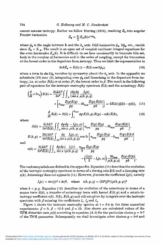
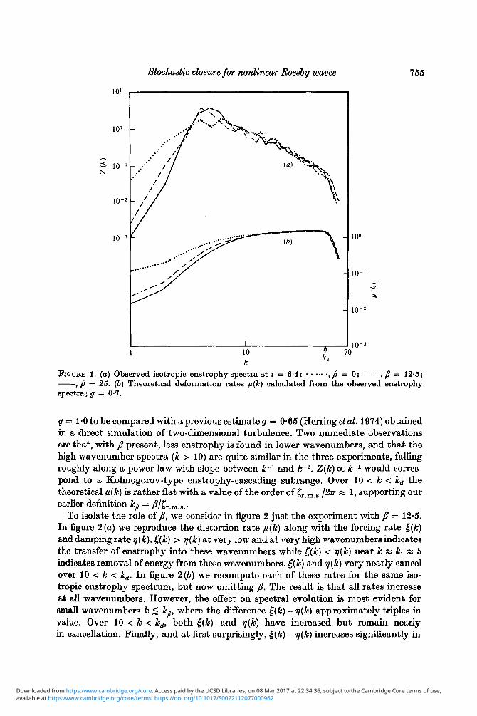
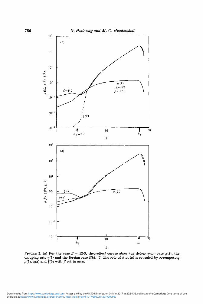
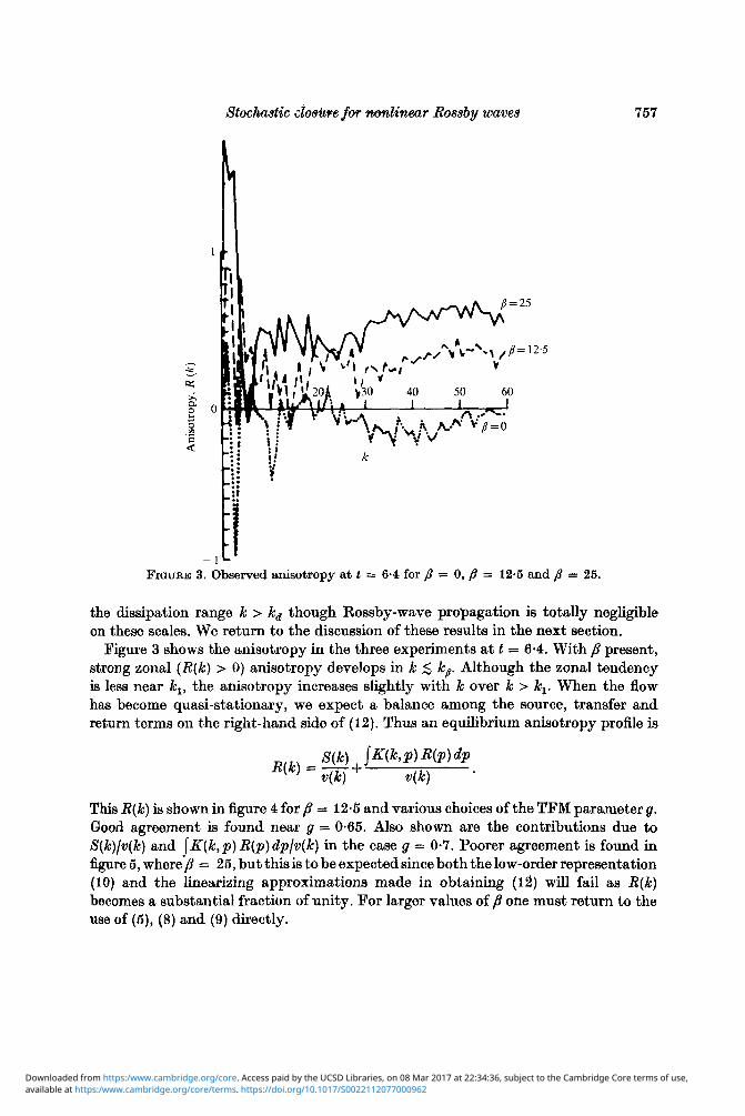
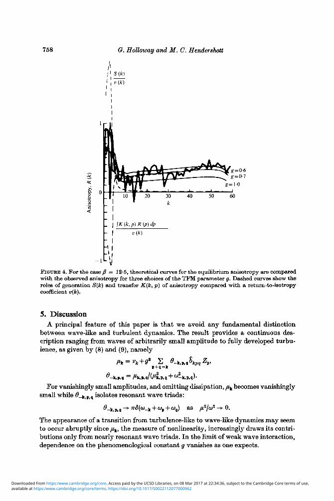
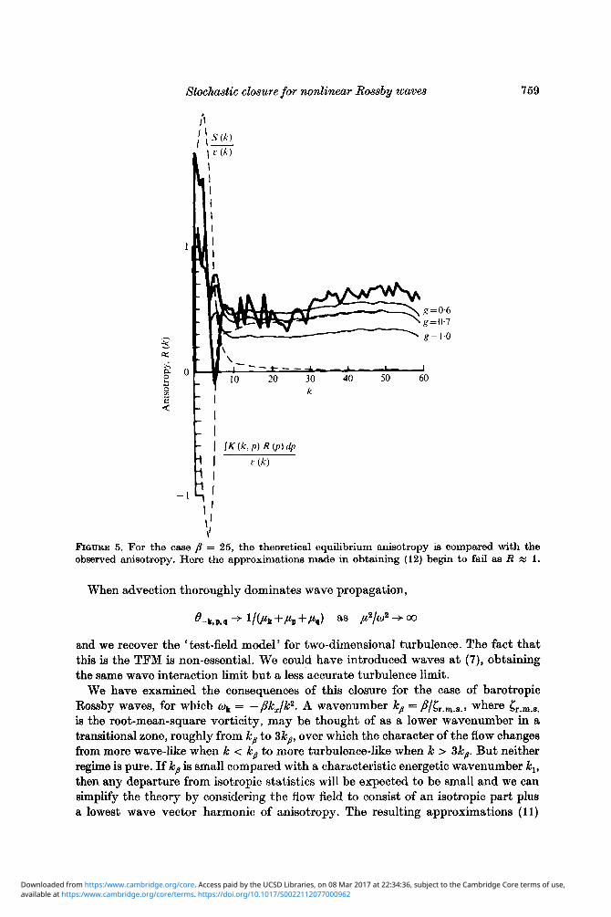
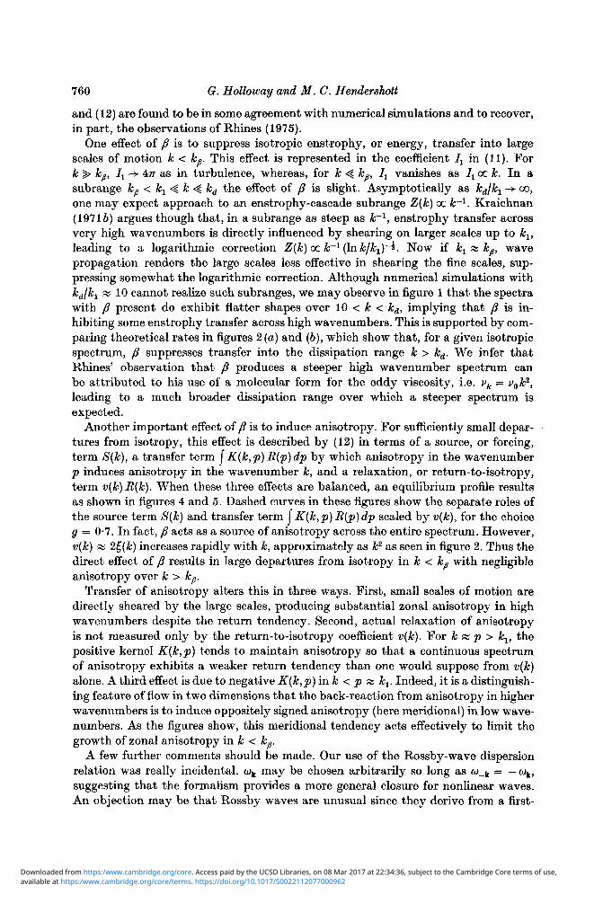
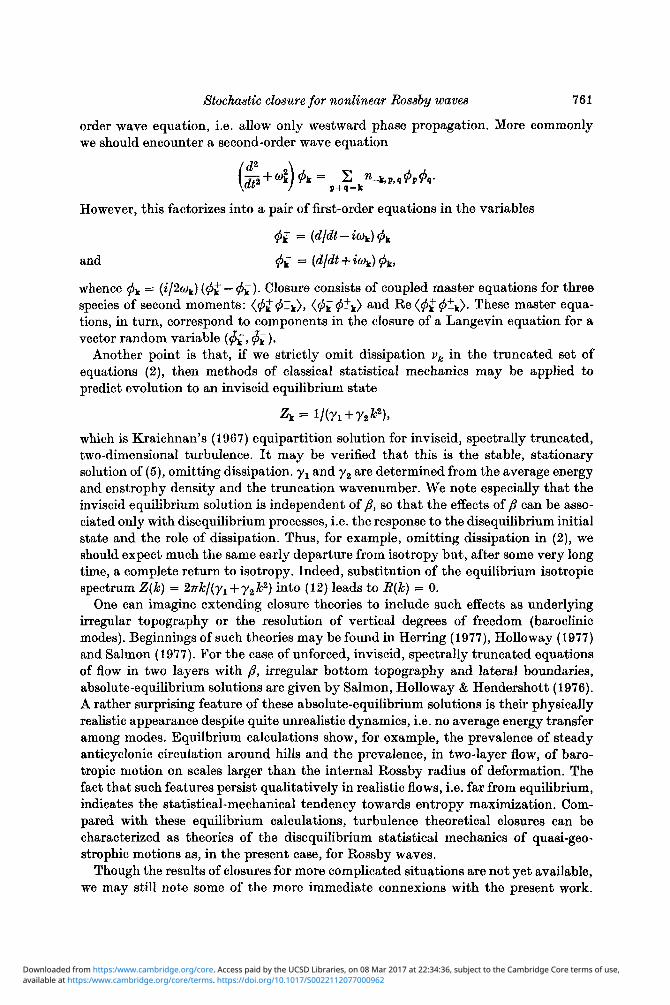
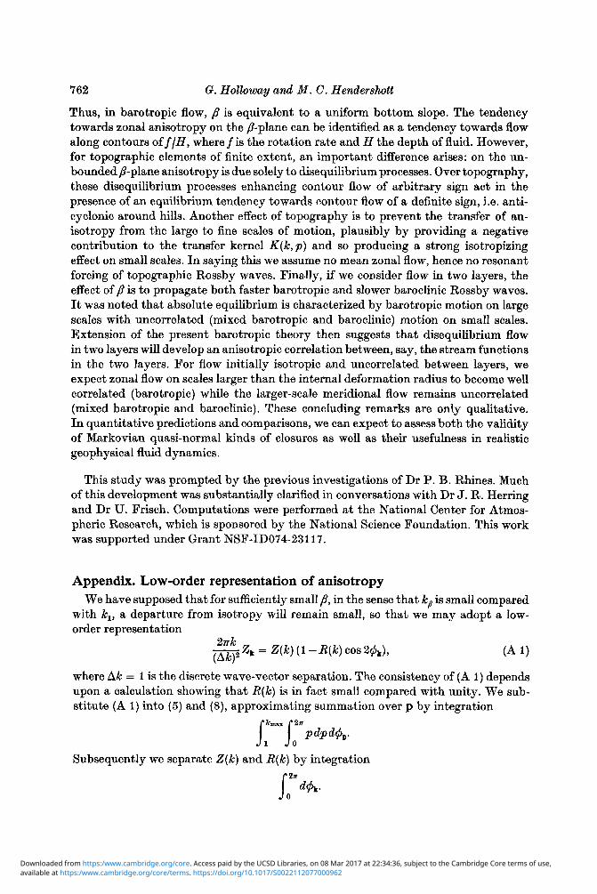
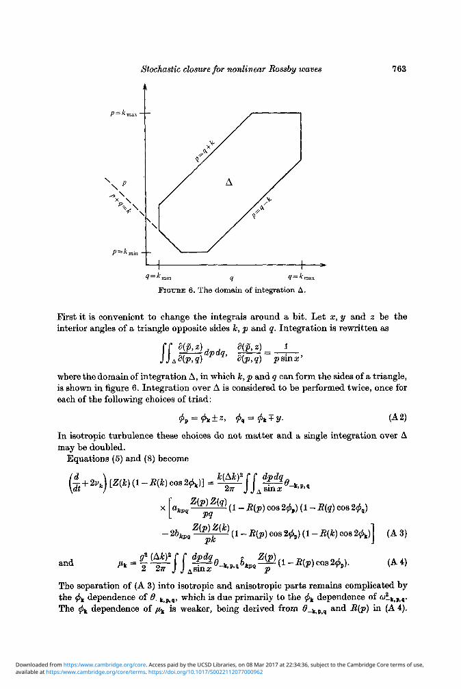


![The Arithmetic Geometry of Resonant Rossby Wave Triads · ARITHMETIC GEOMETRY OF RESONANT ROSSBY WAVE TRIADS 353 tion 3.17 and Chapter 6]). The -plane model was introduced by Rossby](https://img.pdfslide.net/doc/110x75/6065c2e71c4a3a76bc3dd2c3/the-arithmetic-geometry-of-resonant-rossby-wave-triads-arithmetic-geometry-of-resonant.jpg)