Embed Size (px)
Citation preview

Stochastic Dynamics of Financial Markets
A thesis submitted to the University of Manchester for the degree of
Doctor of Philosophy
in the Faculty of Humanities
2013
Mikhail Valentinovich Zhitlukhin
School of Social Sciences/Economic Studies

Contents
Abstract 5
Declaration 6
Copyright Statement 7
Acknowledgements 8
List of notations 9
Introduction 10
Chapter 1. Multimarket hedging with risk 24
1.1. The model of interconnected markets and the hedging principle 25
1.2. Conditions for the validity of the hedging principle . . . . . . . . . . . . . 31
1.3. Risk-acceptable portfolios: examples . . . . . . . . . . . . . . . . . . . . . . . . . . . 38
1.4. Connections between consistent price systems and equivalent
martingale measures . . . . . . . . . . . . . . . . . . . . . . . . . . . . . . . . . . . . . . . . . . . 41
1.5. A model of an asset market with transaction costs and portfolio
constraints . . . . . . . . . . . . . . . . . . . . . . . . . . . . . . . . . . . . . . . . . . . . . . . . . . . . . 43
1.6. Appendix 1: auxiliary results from functional analysis . . . . . . . . . . 52
1.7. Appendix 2: linear functionals in non-separable 𝐿1 spaces . . . . . . 55
Chapter 2. Utility maximisation in multimarket trading 57
2.1. Optimal trading strategies in the model of interconnected asset
markets . . . . . . . . . . . . . . . . . . . . . . . . . . . . . . . . . . . . . . . . . . . . . . . . . . . . . . . . 58
2.2. Supporting prices: the definition and conditions of existence. . . . 62
2.3. Supporting prices in an asset market with transaction costs and
portfolio constraints . . . . . . . . . . . . . . . . . . . . . . . . . . . . . . . . . . . . . . . . . . . 67
2.4. Examples when supporting prices do not exist. . . . . . . . . . . . . . . . . . 70
2.5. Appendix: geometric duality . . . . . . . . . . . . . . . . . . . . . . . . . . . . . . . . . . . 74
2

Chapter 3. Detection of changepoints in asset prices 75
3.1. The problem of selling an asset with a changepoint . . . . . . . . . . . . . 76
3.2. The structure of optimal selling times . . . . . . . . . . . . . . . . . . . . . . . . . . 78
3.3. The proof of the main theorem. . . . . . . . . . . . . . . . . . . . . . . . . . . . . . . . . 81
3.4. Numerical solutions . . . . . . . . . . . . . . . . . . . . . . . . . . . . . . . . . . . . . . . . . . . . 89
References 96
Word count: 31991.
3
List of Figures
Fig. 1. Stopping boundaries for the Shiryaev–Roberts statistic . . . . . . . . . . 93
Fig. 2. Stopping boundaries for the posterior probability process . . . . . . . 93
Fig. 3. Value functions for the Shiryaev–Roberts statistic . . . . . . . . . . . . . . . 94
Fig. 4. Value functions for the posterior probability process . . . . . . . . . . . . 94
Fig. 5. Sample paths of the random walk with changepoints . . . . . . . . . . . . 95
Fig. 6. Paths of the Shiryaev–Roberts statistic . . . . . . . . . . . . . . . . . . . . . . . . . 95
4
The University of Manchester
Mikhail Valentinovich Zhitlukhin
PhD Economics
Stochastic Dynamics of Financial Markets
September 2013
Abstract
This thesis provides a study on stochastic models of financial marketsrelated to problems of asset pricing and hedging, optimal portfolio managingand statistical changepoint detection in trends of asset prices.
Chapter 1 develops a general model of a system of interconnected stochas-tic markets associated with a directed acyclic graph. The main result ofthe chapter provides sufficient conditions of hedgeability of contracts in themodel. These conditions are expressed in terms of consistent price systems,which generalise the notion of equivalent martingale measures. Using thegeneral results obtained, a particular model of an asset market with trans-action costs and portfolio constraints is studied.
In the second chapter the problem of multi-period utility maximisationin the general market model is considered. The aim of the chapter is toestablish the existence of systems of supporting prices, which play the role ofLagrange multipliers and allow to decompose a multi-period constrained util-ity maximisation problem into a family of single-period and unconstrainedproblems. Their existence is proved under conditions similar to those ofChapter 1.
The last chapter is devoted to applications of statistical sequential meth-ods for detecting trend changes in asset prices. A model where prices aredriven by a geometric Gaussian random walk with changing mean and vari-ance is proposed, and the problem of choosing the optimal moment of timeto sell an asset is studied. The main theorem of the chapter describes thestructure of the optimal selling moments in terms of the Shiryaev–Robertsstatistic and the posterior probability process.
5

Declaration
No portion of the work referred to in the thesis has been submitted in
support of an application for another degree or qualification of this or any
other university or other institute of learning.
6

Copyright Statement
The author of this thesis (including any appendices and/or schedules to
this thesis) owns certain copyright or related rights in it (the Copyright)
and he has given The University of Manchester certain rights to use such
Copyright, including for administrative purposes.
Copies of this thesis, either in full or in extracts and whether in hard or
electronic copy, may be made only in accordance with the Copyright, Designs
and Patents Act 1988 (as amended) and regulations issued under it or, where
appropriate, in accordance with licensing agreements which the University
has from time to time. This page must form part of any such copies made.
The ownership of certain Copyright, patents, designs, trade marks and
other intellectual property (the Intellectual Property) and any reproductions
of copyright works in the thesis, for example graphs and tables (Reproduc-
tions), which may be described in this thesis, may not be owned by the
author and may be owned by third parties. Such Intellectual Property and
Reproductions cannot and must not be made available for use without the
prior written permission of the owner(s) of the relevant Intellectual Property
and/or Reproductions.
Further information on the conditions under which disclosure, publica-
tion and commercialisation of this thesis, the Copyright and any Intellec-
tual Property and/or Reproductions described in it may take place is avail-
able in the University IP Policy (see http://www.campus.manchester.ac.uk/
medialibrary/policies/intellectual-property.pdf), in any relevant Thesis re-
striction declarations deposited in the University Library, The University Li-
brary’s regulations (see http://www.manchester.ac.uk/library/aboutus/
regulations) and in The University’s policy on presentation of Theses.
7
Acknowledgements
I owe my deepest gratitude to my supervisors, Professor Igor Evstigneev
and Professor Goran Peskir, for their continuous support of my research, for
the immense knowledge and inspiration they gave me. It was my sincere
pleasure to work with them and I deeply appreciate their help during all the
time of the research and writing the thesis.
I am grateful to Professor Albert Shiryaev, whom I consider my main
teacher in stochastic analysis and probability. It is impossible to overestimate
the importance of his continuous attention to my research and my career.
I am indebted to Professor William T. Ziemba and Professor Sandra
L. Schwartz, who motivated me to study applications of sequential statis-
tical methods to stock markets.
I thank Professor Hans Rudolf Lerche and Dr Pavel Gapeev for the valu-
able discussions of the mathematical problems related to my research.
My study at The University of Manchester was funded by the Economics
Discipline Area Studentship from The School of Social Sciences, which I
greatly acknowledge.
An acknowledgement is also made to the Hausdorff Research Institute
for Mathematics (Bonn, Germany), where I attended trimester program
“Stochastic Dynamics in Economics and Finance” in summer 2013. The
hospitality of HIM and the excellent research environment were invaluable
for the preparation of the thesis. In particular, I thank the organisers of the
program, Professor Igor Evstigneev, Professor Klaus Reiner Schenk-Hoppe
and Professor Rabah Amir.
8

List of notations
R the set of real numbers
R+ the set of non-negative real numbers
𝐿1 the space of all integrable functions on a measure space
𝐿∞ the space of all essentially bounded functions on a measure
space
𝑋* the positive dual cone of a set 𝑋 in a normed space
P | F the restriction of a measure P to a 𝜎-algebra F
𝑥+ max{𝑥, 0}
𝑥− −min{𝑥, 0}
I{𝐴} the indicator of a statement 𝐴 (I{𝐴} = 1 if 𝐴 is true,
I{𝐴} = 0 if 𝐴 is false)
𝒯𝑡+ the set of all successors of a node 𝑡 in a graph 𝒯
𝒯𝑡− the set of all predecessors of a node 𝑡 in a graph 𝒯
𝒯− the set of all nodes in a graph 𝒯 with at least one successor
𝒯+ the set of all nodes in a graph 𝒯 with at least one predecessor
N (𝜇, 𝜎2) Gaussian distribution with mean 𝜇 and variance 𝜎2
Φ the standard Gaussian cumulative distribution function
(Φ(𝑥) = 1√2𝜋
∫ 𝑥
−∞ 𝑒−𝑦2/2𝑑𝑦)
a.s. “almost surely” (with probability one)
i.i.d. independent and identically distributed (random variables)
9

Introduction
This thesis provides a study on stochastic models of financial markets.
Questions of derivatives pricing and hedging, optimal portfolio managing
and detection of changes in asset prices trends are considered.
The first range of questions – hedging and pricing of derivative securities –
has been studied in the literature since 1960s. The celebrated Black–Scholes
formula [3] for the price of a European option was one of the first fundamental
results in this direction. Derivative securities (or contingent claims) play an
important role in modern finance as they allow to implement complex trading
strategies which reduce the risk from indeterminacy of future asset prices.
One of the main questions in derivatives trading consists in determining
the fair price of a derivative, which satisfies both the seller and the buyer.
The Black–Scholes formula provides an explicit answer to this question in the
model when asset prices are modelled by a geometric Brownian motion. Later
this result was extended to a wider class of market models. The development
of the derivatives pricing theory has resulted in that nowadays the volume
of derivatives traded is much higher than the volume of basic assets [41].
The second range of questions considered in the thesis concerns consump-
tion-investment problems, where a trader needs to manage a portfolio of as-
sets choosing how much to consume in order to maximise utility over a period
of time. Questions of this type were originally studied in relation to models
of economic growth, where the objective is to find a trade-off between goods
produced and consumed with the aim of the optimal development of the econ-
omy. One of the first results in the financial context was obtained by Merton
[42], who provided an explicit solution of the consumption-investment prob-
lem for a model when asset prices are driven by a geometric Brownian motion.
There have been several extensions of Merton’s result which include factors
like transaction costs, possibility of bankruptcy, general classes of stochastic
processes describing asset prices, etc. (see e. g. [4, 10, 36, 44]).
10

The third part of the thesis contains applications of sequential methods
of mathematical statistics to detecting changes in asset prices trends. The
mathematical foundation of the corresponding statistical methods – the the-
ory of changepoint detection (or disorder detection) – was laid in the papers
by W. Shewhart, E. S. Page, S.W. Roberts, A.N. Shiryaev, and others in
1920-1960s, and initially was applied in questions of production quality con-
trol and radiolocation. Recently, these methods have gained attention in
finance.
The main results of the thesis generalise the classical theory to advanced
market models. We obtain results that broaden the models available in the
literature and reflect several important features of real markets that have
not been studied earlier in the corresponding fields.
The rest of the introduction provides a detailed description of the prob-
lems considered in the thesis.
Asset pricing and hedging
Consider the classical model of a stochastic financial market, which op-
erates at discrete moments of time 𝑡 = 0, 1, . . . , 𝑇 , and where 𝑁 assets are
traded. The stochastic nature of the market is represented by a filtered
probability space (Ω,F , (F𝑡)𝑇𝑡=0,P), where each 𝜎-algebra F𝑡 in the filtra-
tion F0 ⊂ F1 ⊂ . . .F𝑇 describes random factors that might affect the
market at time 𝑡.
The prices of the assets at time 𝑡 are given by F𝑡-measurable strictly
positive random variables 𝑆1𝑡 , 𝑆
2𝑡 , . . . , 𝑆
𝑁𝑡 . Asset 1 is assumed to be riskless
(e. g. cash deposited with a bank account) with the price 𝑆1𝑡 ≡ 1 (after being
discounted appropriately), while assets 𝑖 = 2, . . . , 𝑁 are risky with random
prices.
An investor can trade in the market by means of buying and selling assets.
A trading strategy is a sequence 𝑥0, 𝑥1, . . . , 𝑥𝑇 of random 𝑁 -dimensional
vectors, where each 𝑥𝑡 = (𝑥1𝑡 , . . . , 𝑥𝑁𝑡 ) is F𝑡-measurable and specifies the
11

portfolio held by the investor between the moments of time 𝑡 and 𝑡+1. The
coordinate 𝑥𝑖𝑡 (𝑖 = 1, . . . , 𝑁) is equal to the amount of physical units of asset
𝑖 in the portfolio.
An important class of trading strategies consists of self-financing trading
strategies, which have no exogenous inflow or outflow of money. Namely, a
trading strategy (𝑥𝑡)𝑡6𝑇 is called self-financing if
𝑥𝑡−1𝑆𝑡 = 𝑥𝑡𝑆𝑡 for each 𝑡 = 1, . . . , 𝑇,
where the left-hand side is the value of the old portfolio (established “yester-
day”), and the right-hand side is the value of the new portfolio (established
“today”). The equality is understood to hold with probability one.
The central question of the derivatives pricing and hedging theory con-
sists in finding fair prices of derivative securities (or contingent claims). A
derivative is a financial instrument which has no intrinsic value in itself,
but derives its value from underlying basic assets [15]. Derivative securities
include options, futures, swaps, and others (see e. g. [31]).
As an example, consider a standard European call option on asset 𝑖, which
is a contract that allows (but does not oblige) its buyer to buy one unit of
asset 𝑖 at a fixed time 𝑇 in the future for a fixed price 𝐾. The seller incurs
a corresponding obligation to fulfil the agreement if the buyer decides to
exercise the contract, which she does if the spot price 𝑆𝑖𝑇 is greater than 𝐾
(thus receiving the gain 𝑆𝑖𝑇 −𝐾). In order to obtain the option, the buyer
pays the seller some premium, the price of the option, at time 𝑡 = 0 .
Another example is a European put option, which is a contract giving its
buyer the right to sell asset 𝑖 at a fixed time 𝑇 for a fixed price 𝐾. If the
buyer exercises the option (which happens whenever 𝐾 > 𝑆𝑖𝑇 ), she receives
the gain 𝐾 − 𝑆𝑖𝑇 .
Mathematically, contracts of this type can be identified with random
variables 𝑋 representing the payoff of the seller to the buyer at time 𝑇 . For
example, 𝑋 = (𝑆𝑇 −𝐾)+ for a European call option, and 𝑋 = (𝐾 − 𝑆𝑇 )+
for a European put option.
It is said that a self-financing trading strategy (𝑥𝑡)𝑡6𝑇 (super)hedges a
12
derivative 𝑋 if
𝑥𝑇𝑆𝑇 > 𝑋 a.s.,
i. e. the seller who follows the strategy (𝑥𝑡)𝑡6𝑇 can fulfil the payment asso-
ciated with the derivative with probability one. The minimal value 𝑥 of the
initial portfolio 𝑥0 is called the (upper) hedging price of 𝑋 and is denoted
by 𝒞(𝑋):
𝒞(𝑋) = inf{𝑥 : there exists (𝑥𝑡)𝑡6𝑇 superhedging 𝑋 such that 𝑥0𝑆0 = 𝑥}.
The price 𝒞(𝑋) is the minimal value of the initial portfolio that allows
the seller to fulfil her obligations (provided that the infimum in the definition
is attained; see [61, Ch. VI, S 1b-c]). On the other hand, if she could sell the
derivative for a higher price 𝒞 > 𝒞(𝑋), it would be possible to find a trading
strategy which delivers her a free-lunch – a non-negative and non-zero gain
by time 𝑇 , for which the buyer has no incentive to agree.
The central result of the asset pricing and hedging theory states that in
a market without arbitrage opportunities the price of a contingent claim can
be found as the supremum of its expected value with respect to equivalent
martingale measures.
It is said that a self-financing trading strategy (𝑥𝑡)𝑡6𝑇 realises an arbitrage
opportunity in the market if
𝑥0𝑆0 = 0, 𝑥𝑇𝑆𝑇 > 0 and P(𝑥𝑇𝑆𝑇 > 0) > 0.
A probability measure P, equivalent to the original measure P (P ∼ P),
is called an equivalent martingale measure (EMM), if the price sequence 𝑆 is
a P-martingale, i. e. EP(𝑆𝑖
𝑡 | F𝑡−1) = 𝑆𝑖𝑡−1 for all 𝑡 = 1, . . . , 𝑇 , 𝑖 = 1, . . . , 𝑁 .
The set of all EMMs is denoted by P(P).
These two notions express some form of market efficiency. The absence
of arbitrage opportunities means that there is no trading strategy with zero
initial capital, which allows to obtain a non-zero gain without downside
risk (a free lunch) at time 𝑇 . The existence of an equivalent martingale
measure allows to change the underlying measure P, preserving the sets of
zero probability, in a way that the assets have zero return rates.
13
Theorem. Equivalent martingale measures exist in a market if and only
if there is no arbitrage opportunities.
In a market without arbitrage opportunities, the price of a contingent
claim 𝑋 such that EP|𝑋| <∞ for any P ∈ P(P) can be found as
𝒞(𝑋) = supP∈P
EP𝑋.
Remark. In the case when there is only one equivalent martingale mea-
sure (the case of a complete market), 𝒞(𝑋) = EP𝑋. It turns out that a
complete market has a simple structure – the 𝜎-algebra F𝑇 is purely atom-
istic with respect to P and consists of no more that 𝑁𝑇 atoms. Note that in
continuous time, however, there exist examples of complete markets where
F𝑇 is not purely atomistic (e. g. the model of geometric Brownian motion).
The above theorem is referred to as the Fundamental Theorem of Asset
Pricing and the Risk-Neutral Pricing Principle (see e. g. [24, 61]). It con-
stitutes the core of the classical derivatives pricing theory. However it does
not take into account several important features of real markets, which are
necessary to consider when applying the theory in practice. The present the-
sis addresses these issues and develops a model that includes the following
improvements.
1. Transaction costs and portfolio constraints. The act of buying or
selling assets in a real market typically reduces the total wealth of a trader
(due to broker’s commission, differences in bid and offer prices, etc.). As
a result, an investor may need to limit the number of trading operations in
order not to lose too much money on transaction costs. Real markets also set
constraints on admissible portfolios in order to prevent market participants
from using too risky trading strategies. For example, such constraints can
be expressed in a form of a margin requirement, which obliges investors to
choose only those strategies that allow to liquidate their portfolios if prices
move unfavourably.
Both transaction costs and portfolio constraints limit investor abilities,
and thus, generally, increase hedging prices. These aspects have already been
14

considered in the literature, but for the most part separately. One can point,
e.g., to the monograph by Kabanov and Safarian [33] discussing transaction
costs, the papers by Jouini, Kallal [32] and Evstigneev, Schurger, Taksar [22]
dealing with portfolio constraints, and the references therein.
It turns out that under the presence of transaction costs and portfolio
constraints, the problem of pricing contingent claims has a solution simi-
lar to the classical model. Namely, the price of a contingent claim can be
found as the supremum of its expected value with respect to consistent price
systems, which are vector analogues of equivalent martingale measures (see
Chapter 1 for details). However, the existence of consistent price systems
in a market with transaction costs and portfolio constraints becomes a con-
siderably difficult question, and, generally, requires conditions stronger than
the absence of arbitrage opportunities. Several stronger conditions have been
introduced in the literature which guarantee the existence of consistent price
systems, thus allowing to price contingent claims. Their formulations can be
found in e.g. [22, 33].
2. Hedging with risk. The classical superhedging condition requires
that the seller of a derivative chooses a trading strategy that covers the
payment with probability one, i. e. without any risk of non-fulfilling her
obligation. However, it may be acceptable for the seller to guarantee the
required amount of payment only with some (high) level of confidence – for
example, in unfavourable outcomes she may use exogenous funds, which is
compensated by a higher gain in favourable outcomes.
This is especially important when the volume of trading is large, so not
the result of every single deal is important, but only the average result of a
large number of them. Weakening the superhedging criterion can possibly
reduce derivatives prices and lead to a potential gain while maintaining an
acceptable level of risk of unfavourable situations.
An approach of hedging with risk, used in the thesis, is based on replac-
ing the superhedging condition with a general principle requiring that the
difference between the required payment and the portfolio used to cover it
belongs to a certain set of acceptable portfolios (the exact formulation will
15

be given in Chapter 1). The superhedging condition is a particular case of
this model.
This approach has already been used in the literature. Especially, much
attention has been devoted to hedging with respect to coherent and convex
risk measures (see e. g. the papers [7, 9], where it is called the no good deals
pricing principle).
3. Multimarket trading. The framework developed in the thesis is
capable of modelling a system of interconnected markets associated with
nodes of a given acyclic directed graph. The nodes of the graph represent
different trading sessions that may be related to different moments of time
and/or different asset markets. In particular, the standard model of a single
market can be represented by the graph being the linearly ordered set of
moments of time, while the general case allows to consider the problem of
distributing assets between several markets, which may operate at the same
or different moments of time.
We also consider contracts with payments at arbitrary trading sessions
(not only the terminal ones), which broadens the range of possible financial
instruments. This also makes the model potentially applicable not only in
finance, but in other areas, e.g. it can be used in insurance, where an insurer
receives a premium at time 𝑡 = 0 and needs to manage a portfolio in order
to be able to cover claims occurring randomly.
The above features of real markets have been studied in the literature
for the most part separately. In the thesis a new general model is proposed,
which incorporates all of them. The central result of the first chapter for the
new model is the hedging criterion formulated in terms of consistent price
systems – direct analogues of equivalent martingale measures. We prove their
existence and show that a contract is hedgeable if and only if its value with
respect to any consistent price system is non-negative. In order to obtain
the result, we systematically use the idea of margin requirements which limit
allowed leverage of admissible portfolios. This differs from the standard
approach based on the absence of arbitrage. However, margin requirements
always present in one form or another in any real market, which makes our
16

approach fully justified from the applied point of view.
The model is based on the framework of von Neumann – Gale dynamical
systems introduced by von Neumann [68] and Gale [25] for deterministic
models of a growing economy, and later extended by Dynkin, Radner and
their research groups to the stochastic case. A model of a financial market
based on von Neumann – Gale systems was also proposed in the paper [11]
for the case of a discrete probability space (Ω,F ,P) and a linearly ordered
set of moments of time.
In the thesis this framework is extended to financial market models, which
have several important distinctions from models of growing economies.
Optimal trading strategies
In the second chapter the problem of finding trading strategies that max-
imise the utility function of an investor over a period of time is studied.
In the financial literature, problems of this type are commonly referred
to as consumption-investment problems, and there exists a large number of
results in this area. The subject of our research is the optimal investment
problem for the general model proposed in Chapter 1. The goal is to obtain
conditions for the existence of supporting prices, which allow to reduce a
multi-period constrained maximisation problem of investor’s utility function
to a family of single-stage unconstrained problems. Supporting prices play
the role similar to that of Lagrange multipliers.
The problem of utility maximisation and existence of supporting prices
plays a central role in the von Neumann – Gale framework of economic
growth. The setting of the problem and the main results there consist in the
following.
A von Neumann – Gale system is a sequence of pairs of random vectors
(𝑥𝑡, 𝑦𝑡) 𝑡 = 0, 1, . . . , 𝑇 , such that (𝑥𝑡, 𝑦𝑡) ∈ 𝒵𝑡 for some given sets 𝒵𝑡, and
𝑥𝑡 6 𝑦𝑡−1. In the financial interpretation, a vector 𝑥𝑡 can be regarded as
a portfolio of assets held before a trading session 𝑡, and 𝑦𝑡 as a portfolio
17

obtained during the session. The inequality 𝑥𝑡 6 𝑦𝑡−1 means that there is
no exogenous infusion of assets (but disposal of assets is allowed). The sets
𝒵𝑡 can describe the self-financing condition, portfolio constraints, etc.
In models of economic growth vectors 𝑥𝑡 describe amounts of input com-
modities for a production process with output commodities 𝑦𝑡. The sets 𝒵𝑡
consist of all possible production processes and the condition 𝑥𝑡 6 𝑦𝑡−1 re-
flects the requirement that the input of any production process should not
exceed the output of the previous one.
Suppose that with each set 𝒵𝑡 a real-valued utility function 𝑢𝑡(𝑥𝑡, 𝑦𝑡) is
associated and interpreted as the utility from the production process with
input commodities 𝑥𝑡 and output commodities 𝑦𝑡. Let 𝑥0 be a given vector of
initial resources. Then the problem consists in finding a production process
𝜁 = (𝑥𝑡, 𝑦𝑡)𝑡6𝑇 , represented by a von Neumann – Gale system, such that
𝑥0 = 𝑥0 and which maximises the utility
𝑢(𝜁) :=𝑇∑𝑡=0
𝑢𝑡(𝑥𝑡, 𝑦𝑡).
This is a constrained maximisation problem of the function 𝑢(𝜁) over
all sequences 𝜁 = (𝑥𝑡, 𝑦𝑡)𝑡6𝑇 with (𝑥𝑡, 𝑦𝑡) ∈ 𝒵𝑡 satisfying the constraints
𝑥𝑡 6 𝑦𝑡−1. Under some assumptions the solution 𝜁* of the problem exists,
and, moreover, there exist random vectors 𝑝𝑡, 𝑡 = 0, . . . , 𝑇 + 1 such that
𝑢(𝜁*) >𝑇∑𝑡=0
(𝑢𝑡(𝑥𝑡, 𝑦𝑡) + E[𝑦𝑡𝑝𝑡+1 − 𝑥𝑡𝑝𝑡]
)+ E𝑥0𝑝0
for any sequence (𝑥𝑡, 𝑦𝑡)𝑡6𝑇 with (𝑥𝑡, 𝑦𝑡) ∈ 𝒵𝑡. Thus 𝜁* solves the uncon-
strained problem of maximising the right hand side of the above inequality.
Moreover, in order to maximise the right-hand size it is sufficient to max-
imise each term 𝑢𝑡(𝑥𝑡, 𝑦𝑡) + E[𝑦𝑡𝑝𝑡+1 − 𝑥𝑡𝑝𝑡] independently. Gale [26] noted
the great importance of results of this type by saying that it is “the single
most important tool in modern economic analysis both from the theoretical
and computational point of view”.
The aim of the second chapter is to obtain similar results for our model
of interconnected financial markets. The main mathematical difficulty here
18

consists in that in our model portfolios (𝑥𝑡, 𝑦𝑡) may have negative coordi-
nates (corresponding to short sales), unlike commodities vectors in models
of economic growth. The key role in establishing the main results of the
second chapter will be played by the assumption of margin requirements.
The existence of supporting prices will be proved under a condition on the
size of the margin.
Detection of trend changes in asset prices
The third part of the thesis studies statistical methods of change detection
in trends of asset prices. We consider a model, where prices initially rise, but
may start falling at a random (and unknown) moment of time. The aim of
an investor is to detect this change in the prices trend and to sell the asset
as close as possible to its highest price.
It will be assumed that the price of an asset is represented by a geometric
Gaussian random walk 𝑆 = (𝑆𝑡)𝑇𝑡=0 defined on a probability space (Ω,F ,P),
whose drift and volatility coefficients may change at an unknown time 𝜃:
𝑆0 > 0, log𝑆𝑡
𝑆𝑡−1=
⎧⎨⎩𝜇1 + 𝜎1𝜉𝑡, 𝑡 < 𝜃,
𝜇2 + 𝜎2𝜉𝑡, 𝑡 > 𝜃,for 𝑡 = 1, 2, . . . , 𝑇,
where 𝜇1, 𝜇2, 𝜎1, 𝜎2 are known parameters, 𝜉𝑡 ∼ N (0, 1) are i.i.d. normal
random variables with zero mean and unit variance, and 𝜃 is the moment of
time when the probabilistic character of the price sequence changes.
In order to model the uncertainty of the moment 𝜃, it will be assumed
that 𝜃 is a random variable defined on (Ω,F ,P), but an investor can observe
only the information included in the filtration F = (F𝑡)𝑇𝑡=0, F𝑡 = 𝜎(𝑆𝑢;𝑢 6
𝑡), generated by the price sequence, and cannot observe 𝜃 directly. The
distribution law of 𝜃 is known, and 𝜃 takes values 1, 2, . . . , 𝑇 with known
probabilities 𝑝𝑡 > 0, so that𝑇∑𝑡=1
𝑝𝑡 6 1. The quantity 𝑝𝑇+1 = 1−𝑇∑𝑡=1
𝑝𝑡 is the
probability that the change of the parameters does not occur until the final
19
time 𝑇 and 𝑝1 is the probability that the logarithmic returns already follow
N (𝜇2, 𝜎2) since the initial moment of time.
By definition, a moment 𝜏 when one can sell the asset should be a stopping
time of the filtration F, which means that {𝜔 : 𝜏(𝜔) 6 𝑡} ∈ F𝑡 for any
0 6 𝑡 6 𝑇 . The notion of a stopping time expresses the idea that the
decision to sell the asset at time 𝑡 should be based only on the information
available from the price history up to time 𝑡, and does not rely on future
prices. The class of all stopping times 𝜏 6 𝑇 of the filtration F is denoted
by M.
The problem we consider consists in maximising the power or logarithmic
utility from selling the asset. Namely, let 𝑈𝛼(𝑥) = 𝛼𝑥𝛼 for 𝛼 = 0 and
𝑈0(𝑥) = log 𝑥. For an arbitrary 𝛼 ∈ R we consider the optimal stopping
problem
𝑉𝛼 = sup𝜏∈M
E𝑈𝛼(𝑆𝜏 ).
The problem consists in finding the value 𝑉𝛼, which is the maximum expected
utility one can obtain from selling the asset, and finding the stopping time
𝜏 *𝛼 at which the supremum is attained (we show that it exists).
The study of methods of detecting changes in probabilistic structure
of random sequences and processes (called disorder detection problems or
changepoint detection problems) began in the 1950-1960s in the papers by
E. Page, S. Roberts, A.N. Shiryaev and others (see [45, 46, 49, 57–59]); the
method of control charts proposed by W.A. Shewhart in the 1920s [55] is
also worth mentioning.
A financial application of changepoint detection methods was considered
in the paper [2] by M. Beibel and H.R. Lerche, who studied the problem
of choosing the optimal time to sell the asset in continuous time, when the
asset price process 𝑆 = (𝑆𝑡)𝑡>0 is modelled by a geometric Brownian motion
whose drift changes at time 𝜃:
𝑑𝑆𝑡 = 𝑆𝑡[𝜇1I(𝑡 < 𝜃) + 𝜇2I(𝑡 > 𝜃)]𝑑𝑡+ 𝜎𝑆𝑡𝑑𝐵𝑡, 𝑆0 > 0,
where 𝐵 = (𝐵𝑡)𝑡>0 is a standard Brownian motion on a probability space
(Ω,F ,P), and 𝜇1, 𝜇2, 𝜎 are known real parameters. The paper [2] assumes
20

that 𝜃 is an exponentially distributed random variable with a known param-
eter 𝜆 > 0 and is independent of 𝐵. An investor looks for the stopping time
𝜏 * of the filtration generated by the process 𝑆 that maximises the expected
gain E𝑆𝜏 (the time horizon in the problem is 𝑇 = ∞, i. e. 𝜏 can be un-
bounded). By changing the parameters 𝜇1, 𝜇2, 𝜎 one can solve the problem
of maximising E𝑆𝛼𝜏 for any 𝛼 except 𝛼 = 0.
Beibel and Lerche show that if 𝜇1, 𝜇2, 𝜎 satisfy some relation, then the
optimal stopping time 𝜏 * can be found as the first moment of time when the
posterior probability process 𝜋 = (𝜋𝑡)𝑡>0, 𝜋𝑡 = P(𝜃 6 𝑡 | F𝑡), exceeds some
level 𝐴 = 𝐴(𝜇1, 𝜇2, 𝜎, 𝜆):
𝜏 * = inf{𝑡 > 0 : 𝜋𝑡 > 𝐴}.
In other words, the optimal stopping time has a very clear interpretation:
one needs to sell the asset as soon as the posterior probability that the change
has happened exceeds a certain threshold. An explicit representation of 𝜋𝑡
through the observable process 𝑆𝑡 is available (see e. g. [47, Section 22]).
In the paper [14] the conditions on 𝜇1, 𝜇2, 𝜎 were relaxed and it was
shown that the result holds for all possible values of the parameters (except
some trivial cases). Also, the optimal threshold was found explicitly as
𝐴 = 𝐴′/(1 + 𝐴′), where the constant 𝐴′ = 𝐴′(𝜇1, 𝜇2, 𝜎, 𝜆) is the unique
positive root of the (algebraic) equation
2
∫ ∞
0
𝑒−𝑎𝑡𝑡(𝑏+𝛾−3)/2(1 + 𝐴′𝑡)𝛾−𝑏+1)/2𝑑𝑡
= (𝛾 − 𝑏+ 1)(1 + 𝐴′)
∫ ∞
0
𝑒−𝑎𝑡𝑡(𝑏+𝛾−1)/2(1 + 𝐴′𝑡)(𝛾−𝑏−1)/2𝑑𝑡
with the parameters
𝑎 =2𝜆
𝜈2, 𝑏 =
2
𝜈
(𝜆
𝜈− 𝜎
), 𝛾 =
√(𝑏− 1)2 + 4𝑐,
where
𝜈 =𝜇2 − 𝜇1
𝜎, 𝑐 =
2(𝜆− 𝜇2)
𝜈2.
The paper [56] studied the problem of maximising the logarithmic utility
21

from selling the asset with finite time horizon 𝑇 (but still assuming that 𝜃
is exponentially distributed, so the parameters do not change until the end
of the time horizon with positive probability). The solution was based on
an earlier result of the paper [28]. It was shown that the optimal stopping
time can be expressed as the first moment of time when 𝜋𝑡 exceeds some
time-dependent threshold:
𝜋𝑡 = inf{𝑡 > 0 : 𝜋𝑡 > 𝑎*(𝑡)},
where 𝑎*(𝑡) is a function on [0, 𝑇 ], dependent on 𝜆, 𝜇1, 𝜇2, 𝜎. The authors
showed that it can be found as a solution of some nonlinear integral equation.
They also briefly discussed the optimal stopping problem for the linear utility
function with a finite time horizon, and reduced it to some two-dimensional
optimal stopping problem for the process 𝜋𝑡, but did not provide its explicit
solution.
The problem on a finite time horizon was solved in the paper [69] by
M.V. Zhitlukhin and A.N. Shiryaev for the both logarithmic and linear
utility functions, provided that 𝜃 is uniformly distributed on [0, 𝑇 ] (however,
the solution can be generalised to a wide class of prior distributions of 𝜃). In
each problem, the optimal stopping time can be expressed as the first time
when the value of 𝜋𝑡 exceeds some function 𝑎*(𝑡) characterised by a certain
integral equation. These equations can be solved numerically by “backward
induction” as demonstrated in the paper.
This result was used by A.N. Shiryaev, M.V. Zhitlukhin and W.T.
Ziemba in the research [66] on stock prices bubbles of Internet related com-
panies. The method of changepoint detection was applied to the daily closing
prices of Apple Inc. in 2009–2012 and the daily closing values of NASDAQ-
100 index in 1994–2002. These two assets had spectacular runs from their
bottom values and dramatic falls after reaching the top values, thus being
good candidates to be modelled by processes with changepoints in trends.
For specific dates of entering the market, the method provided exit points at
approximately 75% of the maximum value of the NASDAQ-100 index, and
90% of the maximum price of Apple Inc. stock.
22
The aim of the third chapter of the thesis is to solve the optimal stopping
problem for a geometric Gaussian random walk with a changepoint in dis-
crete time and a finite time horizon for an arbitrary prior distribution of 𝜃.
It will be shown that the optimal stopping time can be expressed as the first
moment of time when the sequence of the Shiryaev–Roberts statistic (which
is obtained from the posterior probability sequence by a simple transforma-
tion) exceeds some time-dependent level. This result is similar to the results
available in the literature for the case of continuous time. However it allows
to consider any prior distribution of 𝜃 (not only exponential or uniform) and
can be used in models where also the volatility coefficient 𝜎 changes.
A backward induction algorithm for computing the optimal stopping level
is described in the chapter. Using it, we present numerical simulations of
random sequences with changepoints and obtain the corresponding optimal
stopping times.
23
Chapter 1
Multimarket hedging with risk
The results of this chapter extend the classical theory of asset pricing and
hedging in several directions. We develop a general model including transac-
tion costs and portfolio constraints and consider hedging with risk, which is
“softer” than the classical superreplication approach. These aspects of the
modelling of asset markets have already been considered in the literature,
but for the most part separately. One can point, e.g., to the monograph by
Kabanov and Safarian [33] discussing transaction costs, the papers by Jouini
and Kallal [32] and Evstigneev, Schurger and Taksar [22] dealing with portfo-
lio constraints and the studies by Cochrane and Saa-Requejo [9] and Cherny
[7] involving hedging with risk. However, up to now no general model re-
flecting all these features of real financial markets has been proposed.
Another novel aspect of this study is that, in contrast with the conven-
tional theory, we consider asset pricing and hedging in a system of intercon-
nected markets. These markets (functioning at certain moments of discrete
time) are associated with nodes of a given acyclic directed graph. The model
involves stochastic control of random fields on directed graphs. Control prob-
lems of this kind were considered in the context of modelling economies with
locally interacting agents in the series of papers by Evstigneev and Taksar
[16–20].
In the case of a single market – when the graph is a linearly ordered set
of moments of time – the model extends the one proposed by Dempster,
Evstigneev and Taksar [11]. The approach of [11] was inspired by a paral-
lelism between dynamic securities market models and models of economic
growth. The underlying mathematical structures in both modelling frame-
works are related to von Neumann-Gale dynamical systems (von Neumann
[68], Gale [25]) characterised by certain properties of convexity and homo-
24

geneity. This parallelism served as a conceptual guideline for developing the
model and obtaining the results.
The main results of the chapter provide general hedging criteria stated
in terms of consistent price systems, generalising the notion of an equivalent
martingale measure. Existence theorems for such price systems are counter-
parts of various versions of the well-known Fundamental Theorem of Asset
Pricing (Harrison, Kreps, Pliska and others). However, the assumptions we
impose to obtain hedging criteria are substantially distinct from the standard
ones. We systematically use the idea of margin requirements on admissible
portfolios, setting limits for the allowed leverage. Such requirements are
present in one form or another in all real financial markets. Being fully jus-
tified from the applied point of view, they make it possible to substantially
broaden the frontiers of the theory.
The chapter is organised as follows. In Section 1.1 we introduce the gen-
eral model. In Section 1.2 we state and prove the main results. Section 1.3
contains examples of general hedging conditions, and Section 1.4 explains the
connection between consistent price systems and equivalent martingale mea-
sures. By using the general results obtained, we study a specialised model
of a stock market in Section 1.5. Several auxiliary results from functional
analysis are assembled in Sections 1.6 and 1.7.
A shortened version of this chapter was published in the paper [23].
1.1 The model of interconnected markets and the hedging
principle
Let (Ω,F ,P) be a probability space and 𝐺 a directed acyclic graph with
a finite set of nodes 𝒯 . The nodes of the graph represent different trading
sessions that may be related to different moments of time and/or different
asset markets. With each 𝑡 ∈ 𝒯 a 𝜎-algebra F𝑡 ⊂ F is associated describing
random factors that might affect the trading session 𝑡.
A measurable space (Θ,J , 𝜇) with a finite measure 𝜇 is given, whose
25

points represent all available assets. If Θ is infinite, the model reflects the
idea of a “large” asset market (cf. Hildenbrand [30]). For each 𝑡 ∈ 𝒯 , a real-
valued (P⊗ 𝜇)-integrable (F𝑡 ⊗ J )-measurable function 𝑥 : Ω× Θ → R is
interpreted as a portfolio of assets that can be bought or sold in the trading
session 𝑡. The space of all (equivalence classes of) such functions with the
norm ‖𝑥‖ =∫|𝑥|𝑑(P⊗ 𝜇) is denoted by 𝐿1
𝑡 (Ω×Θ) or simply 𝐿1𝑡 . The value
𝑥(𝜔, 𝜃) of a function 𝑥 represents the number of “physical units” of asset 𝜃
in the portfolio 𝑥. Positive values 𝑥(𝜔, 𝜃) are referred to as long positions,
while negative ones as short positions of the portfolio.
If 𝜉 is an integrable real-valued measurable function defined on some
measure space, by E𝜉 we denote the value of its integral over the whole space
(when the measure is a probability measure, E𝜉 is equal to the expectation
of 𝜉).
For a subset 𝑇 ⊂ 𝒯 we denote by 𝐿1𝑇 (Ω×Θ), or simply 𝐿1
𝑇 , the space of
functions 𝑦 : 𝑇 ×Ω×Θ → 𝑅 with finite norm ‖𝑦‖ =∑𝑡∈𝑇
∫|𝑦(𝑡, 𝜔, 𝜃)|𝑑(P⊗𝜇).
Where it is convenient, we represent such functions as families 𝑦 = (𝑦𝑡)𝑡∈𝑇
of functions 𝑦𝑡(𝜔, 𝜃) = 𝑦(𝑡, 𝜔, 𝜃).
The symbols 𝒯𝑡− and 𝒯𝑡+ will be used to denote, respectively, the sets of
all direct predecessors and successors of a node 𝑡 ∈ 𝒯 , and 𝒯−, 𝒯+ will stand,
respectively, for the set of all nodes having at least one successor and the
set of all nodes having at least one predecessor (so that 𝒯− =⋃𝑡∈𝒯
𝒯𝑡− and
𝒯+ =⋃𝑡∈𝒯
𝒯𝑡+). For the convenience of further notation we define 𝐿1𝑡+ = 𝐿1
𝒯𝑡+
for each 𝑡 ∈ 𝒯−, and 𝐿1𝑡− = 𝐿1
𝒯𝑡− for each 𝑡 ∈ 𝒯+.In a trading session 𝑡 ∈ 𝒯− one can buy and sell assets and distribute
them between trading sessions 𝑢 ∈ 𝒯𝑡+. This distribution is specified by a
set of portfolios 𝑦𝑡 = (𝑦𝑡,𝑢)𝑢∈𝒯𝑡+ ∈ 𝐿1𝑡+, where 𝑦𝑡,𝑢 is the portfolio delivered
to the session 𝑢.
Trading constraints in the model are defined by some given (convex)
cones 𝒵𝑡 ⊂ 𝐿1𝑡 ⊗ 𝐿1
𝑡+, 𝑡 ∈ 𝒯−. A trading strategy 𝜁 is a family of functions
𝜁 = (𝑥𝑡, 𝑦𝑡)𝑡∈𝒯− such that
(𝑥𝑡, 𝑦𝑡) ∈ 𝒵𝑡 for each 𝑡 ∈ 𝒯−.
26

Each function 𝑥𝑡 represents the portfolio held before one buys and sells assets
in the session 𝑡. For 𝑡 ∈ 𝒯−, the function 𝑦𝑡 = (𝑦𝑡,𝑢)𝑢∈𝒯𝑡+ specifies the
distribution of assets to the sessions 𝑢 ∈ 𝒯𝑡+.Let 𝑦𝑡− =
∑𝑢∈𝒯𝑡−
𝑦𝑢,𝑡 denote the portfolio of assets delivered to a trading
session 𝑡 from other sessions (𝑦𝑡− := 0 if 𝑡 is a source, i.e. has no predecessors).
In each session 𝑡 ∈ 𝒯 , the portfolio 𝑦𝑡− − 𝑥𝑡 can be used for the hedging of a
contract (we define 𝑥𝑡 = 0 if 𝑡 is a sink, i.e. 𝑡 /∈ 𝒯−). By definition, a contract
𝛾 is a family of portfolios
𝛾 = (𝑐𝑡)𝑡∈𝒯 , 𝑐𝑡 ∈ 𝐿1𝑡 ,
where 𝑐𝑡 stands for the portfolio which has to be delivered – according to
the contract – at the trading session 𝑡. The value of 𝑐𝑡(𝜔, 𝜃) can be negative;
in this case the corresponding amount of asset 𝜃 is received rather than
delivered. The notion of a contract encompasses contingent claims, derivative
securities, insurance contracts, etc.
Assume that a non-empty closed cone 𝒜 ⊂ 𝐿1𝒯 is given. We say that a
trading strategy 𝜁 = (𝑥𝑡, 𝑦𝑡)𝑡∈𝒯− hedges a contract 𝛾 = (𝑐𝑡)𝑡∈𝒯 if
(𝑎𝑡)𝑡∈𝒯 ∈ 𝒜, where 𝑎𝑡 = 𝑦𝑡− − 𝑥𝑡 − 𝑐𝑡. (1.1)
Each 𝑎𝑡 represents the difference between the portfolio 𝑦𝑡− − 𝑥𝑡 delivered at
the session 𝑡 by the strategy 𝜁 and the portfolio 𝑐𝑡 that must be delivered
according to the contract 𝛾. The cone 𝒜 is interpreted as the set of all
risk-acceptable families of portfolios. If 𝒜 is the cone of all non-negative
functions, then 𝜁 is said to superhedge (superreplicate) 𝛾. General cones 𝒜make it possible to consider hedging with risk.
A contract is called hedgeable if there exists a trading strategy hedging it.
The main aim of our study is to characterise the class of hedgeable contracts.
Let 𝐿∞𝑡 = 𝐿∞
𝑡 (Ω×Θ) denote the space of all essentially bounded F𝑡⊗J -
measurable functions 𝑝 : Ω×Θ → R, and 𝒜+ = 𝒜∖(−𝒜) stand for the set of
strictly risk-acceptable families of portfolios (if 𝛼 ∈ 𝒜+, then 𝛼 is acceptable
but −𝛼 is not acceptable).
The characterisation of hedgeable contracts will be given in terms of (mar-
27
ket) consistent price systems that are, by definition, families 𝜋 = (𝑝𝑡)𝑡∈𝒯 of
functions 𝑝𝑡 ∈ 𝐿∞𝑡 (Ω×Θ) satisfying the properties
E𝑥𝑡𝑝𝑡 >∑𝑢∈𝒯𝑡+
E𝑦𝑡,𝑢𝑝𝑢 for each (𝑥𝑡, 𝑦𝑡) ∈ 𝒵𝑡 and 𝑡 ∈ 𝒯−, (1.2)
∑𝑡∈𝒯
E𝑎𝑡𝑝𝑡 > 0 for each 𝛼 = (𝑎𝑡)𝑡∈𝒯 ∈ 𝒜+. (1.3)
Property (1.2) means that it is impossible to obtain strictly positive ex-
pected profit E(∑
𝑢∈𝒯𝑡+𝑦𝑡,𝑢𝑝𝑢 − 𝑥𝑡𝑝𝑡), which is computed in terms of the prices
𝑝𝑡, in the course of trading, as long as the trading constraints are satisfied.
Condition (1.3) is a non-degeneracy assumption, saying that the expected
value of any strictly risk-acceptable family of portfolios is strictly positive.
Throughout the chapter, we suppose that the cone 𝒜 satisfies the follow-
ing assumption.
Assumption (A). 𝒜+ = ∅ and there exists 𝜋 = (𝑝𝑡)𝑡∈𝒯 , 𝑝𝑡 ∈ 𝐿∞𝑡 ,
satisfying (1.3).
The assumption states that there exists an 𝐿1𝒯 -continuous linear func-
tional strictly positive on 𝒜+ = ∅. Its existence for any closed 𝒜 with
𝒜+ = ∅ can be established, e.g., when 𝐿1𝒯 (Ω× Θ) is separable (see Remark
1.6 in Section 1.6).
Our main results, given in the next section, provide conditions guaran-
teeing that the following principle holds.
Hedging principle. The class of consistent price systems is non-empty,
and a contract (𝑐𝑡)𝑡∈𝒯 is hedgeable if and only if∑𝑡∈𝒯
E𝑐𝑡𝑝𝑡 6 0 for all consis-
tent price systems (𝑝𝑡)𝑡∈𝒯 .
The hedging principle states that a contract is hedgeable if and only if its
value in any consistent price system is non-positive. This principle extends
various hedging (and pricing) results available in the literature (cf. e.g. [61,
Ch. V.5, VI.1], [33, Ch. 2.1, 3.1–3.3]).
Note that unlike the classical frictionless asset pricing and hedging theory,
we do not aim to find the price of a contract – in the general model it may be
unclear what can be called the price of a contract (for example, there may be
28

no “basic” asset in terms of which the price can be expressed, or, due to the
possible presence of transaction costs, a portfolio may have different bid and
offer prices). However, if one chooses a particular method of computing the
price of a portfolio, then the price of a contract can be found as the infimum
over the set of the prices of the initial portfolios of trading strategies hedging
this contract. Consequently, the problem of establishing the validity of the
hedging principle can be considered to be more general than the problem of
finding contracts prices.
We conclude this section by several remarks about the properties of con-
sistent price systems.
Remark 1.1. It is useful to observe that condition (1.3) implies that
the price of any risk-acceptable family of portfolios is non-negative with
respect to any consistent price system, i. e. E𝛼𝜋 :=∑𝑡∈𝒯
E𝑎𝑡𝑝𝑡 > 0 for any
consistent price system 𝜋 = (𝑝𝑡)𝑡∈𝒯 and any 𝛼 = (𝑎𝑡)𝑡∈𝒯 ∈ 𝒜. Indeed,
suppose the contrary: E𝛼𝜋 < 0 for some 𝜋 and 𝛼. Consider any 𝛼′ ∈ 𝒜+.
Then 𝑟𝛼+ 𝛼′ ∈ 𝒜+ for any real 𝑟 > 0, while E(𝑟𝛼+ 𝛼′)𝜋 < 0 for all 𝑟 large
enough, which contradicts condition (1.3).
Remark 1.2. The interpretation of a consistent price system (𝑝𝑡)𝑡∈𝒯 as a
system of prices is justified if each 𝑝𝑡 is strictly positive (𝑝𝑡 > 0, P⊗𝜇-a.s.). Asimple sufficient condition for that is when the cone 𝒜 contains all sequences
(𝑎𝑡)𝑡∈𝒯 of non-negative functions 𝑎𝑡 and does not contain any sequence of
non-positive 𝑎𝑡 except the zero one. Another mild condition is provided by
the following proposition.
Proposition 1.1. Each 𝑝𝑡 is strictly positive if the following two condi-
tions hold:
(a) for any 𝑡 ∈ 𝒯− and 0 6 𝑥𝑡 ∈ 𝐿1𝑡 , P(𝑥𝑡 = 0) > 0, there exists 0 6 𝑦𝑡 ∈
𝐿1𝒯𝑡+, P(𝑦𝑡 = 0) > 0, such that (𝑥𝑡, 𝑦𝑡) ∈ 𝒵𝑡;
(b) for any 𝑡 ∈ 𝒯 ∖ 𝒯− and 0 6 𝑎𝑡 ∈ 𝐿1𝑡 , P(𝑎𝑡 = 0) > 0, we have (𝑎′𝑢)𝑢∈𝒯 ∈
𝒜+ if 𝑎′𝑡 = 𝑎𝑡 and 𝑎′𝑢 = 0 for 𝑢 = 𝑡.
In other words, (a) means that it is possible to distribute a non-negative
non-zero portfolio 𝑥𝑡 into non-negative portfolios 𝑦𝑡,𝑢 at least one of which
29

is non-zero; and (b) means that a sequence of portfolios with only one non-
zero portfolio 𝑎𝑡, where 𝑡 is a sink node, is strictly risk-acceptable if 𝑎𝑡 is
non-negative.
Proof. Denote by 𝒯 𝑘 the set {𝑡 ∈ 𝒯 : 𝜅(𝑡) = 𝐾 − 𝑘}, where 𝐾 is the
maximal length of a directed path in the graph and 𝜅(𝑡) is the maximal
length of a directed path emanating from a node 𝑡. The sets 𝒯 0, 𝒯 1, . . . , 𝒯 𝐾
form a partition of 𝒯 such that if there is a path from 𝑡 ∈ 𝒯 𝑘 to 𝑢 ∈ 𝒯 𝑛,
then 𝑘 < 𝑛. Also, note that 𝒯 − = 𝒯 0 ∪ 𝒯 1 ∪ . . . ∪ 𝒯 𝐾−1.
The proposition is proved by induction over 𝑘 = 𝐾,𝐾−1, . . . , 0. For any
𝑡 ∈ 𝒯 𝐾 and 𝑎𝑡 as in (b), from (1.3) we have E𝑎𝑡𝑝𝑡 > 0, so 𝑝𝑡 > 0. Suppose
𝑝𝑠 > 0 for any 𝑠 ∈⋃𝑛>𝑘
𝒯 𝑛. Then for arbitrary 𝑡 ∈ 𝒯 𝑘−1, according to (a), for
any 0 6 𝑥𝑡 ∈ 𝐿1𝑡 , P(𝑥𝑡 = 0) > 0, we can find 0 6 𝑦𝑡 ∈ 𝐿1
𝒯𝑡+ such that P(𝑦𝑡 =0) > 0 and (𝑥𝑡, 𝑦𝑡) ∈ 𝒵𝑡. Inequality (1.2) implies E𝑥𝑡𝑝𝑡 >
∑𝑢∈𝒯𝑡+
E𝑦𝑡,𝑢𝑝𝑢 > 0,
and hence 𝑝𝑡 > 0.
Remark 1.3. Some comments on the relations between the above frame-
work and the von Neumann – Gale model of economic growth [1, 21, 25, 68]
are in order.
In the latter, elements (𝑥𝑡, 𝑦𝑡) in the cones 𝒵𝑡, 𝑡 = 1, 2, . . ., are interpreted
as feasible production processes, with input 𝑥𝑡 and output 𝑦𝑡. Coordinates of
𝑥𝑡, 𝑦𝑡 represent amounts of commodities. The cones 𝒵𝑡 are termed technology
sets. The counterparts of contracts in that context are consumption plans
(𝑐𝑡)𝑡. Sequences of 𝑧𝑡 = (𝑥𝑡, 𝑦𝑡) ∈ 𝒵𝑡, 𝑡 = 1, 2, . . ., are called production plans.
The inequalities 𝑦𝑡−1 − 𝑥𝑡 > 𝑐𝑡, 𝑡 = 1, 2, . . . (analogous to the hedging condi-
tion (1.1)) mean that the production plan (𝑧𝑡) guarantees the consumption
of 𝑐𝑡 at each date 𝑡. Consistent price systems are analogues of sequences of
competitive prices in the von Neumann – Gale model.
30

1.2 Conditions for the validity of the hedging principle
This section contains the formulations and the proofs of the general results
related to the model described in the previous section.
We will use the notation 𝑥+ = max{𝑥, 0}, 𝑥− = −min{𝑥, 0}. We write
“a.s.” if some property holds for P⊗ 𝜇-almost all (𝜔, 𝜃). We say that a set
𝒜 ⊂ 𝐿1 is closed with respect to 𝐿1-bounded a.s. convergence if for any
sequence 𝛼𝑖 = (𝑎𝑖𝑡)𝑡∈𝒯 ∈ 𝒜 such that sup𝑖 ‖𝛼𝑖‖ < ∞ and 𝛼𝑖 → 𝛼 a.s., we
have 𝛼 ∈ 𝒜. In particular, this implies the closedness of 𝒜 in 𝐿1 because
from any sequence converging in 𝐿1 it is possible to extract a subsequence
converging with probability one.
Theorem 1.1. The hedging principle holds if the cones 𝒜 and 𝒵𝑡, 𝑡 ∈𝒯−, are closed with respect to 𝐿1-bounded a.s. convergence and there exist
functions 𝑠1𝑡 ∈ 𝐿∞𝑡 , 𝑠2𝑡,𝑢 ∈ 𝐿∞
𝑡 , 𝑡 ∈ 𝒯−, 𝑢 ∈ 𝒯𝑡+, with values in [𝑠, 𝑠], where
𝑠 > 0, 𝑠 > 1, and a constant 0 6 𝑚 < 1 such that for all 𝑡 ∈ 𝒯−, 𝑢 ∈ 𝒯𝑡+,(𝑥𝑡, 𝑦𝑡) ∈ 𝒵𝑡, and (𝑎𝑟)𝑟∈𝒯 ∈ 𝒜, the following conditions are satisfied:
(a) E𝑥𝑡𝑠1𝑡 > E𝑦𝑡,𝑢𝑠
2𝑡,𝑢;
(b) 𝑚E𝑦+𝑡,𝑢𝑠2𝑡,𝑢 > E𝑦−𝑡,𝑢𝑠
2𝑡,𝑢;
(c) 𝑚E𝑥+𝑡 𝑠1𝑡 > E𝑥−𝑡 𝑠
1𝑡 ;
(d) E𝑎𝑡𝑠1𝑡 > 0.
The functions 𝑠1𝑡 (𝜔, 𝜃) and 𝑠2𝑡,𝑢(𝜔, 𝜃) can be interpreted as some systems of
asset prices. Condition (a) means that in the course of trading the portfolio
value cannot increase “too much”, at least on average. In specific examples,
this assumption follows from the condition of self-financing. Conditions (b)
and (c) express a margin requirement, saying that the total short position
of any admissible portfolio should not exceed on average 𝑚 times the total
long position (cf. e.g. [29]). Condition (d) states that the expectation of the
value (in terms of the price system 𝑠1𝑡 ) of any portfolio in a risk-acceptable
family is non-negative.
The proof of the theorem is based on a lemma. Below we denote by ℋthe set of all hedgeable contracts.
31
Lemma 1.1. For any 𝜋 = (𝑝𝑡)𝑡∈𝒯 , 𝑝𝑡 ∈ 𝐿∞𝑡 , such that E𝛼𝜋 > 0 for every
𝛼 ∈ 𝒜+, the following conditions are equivalent:
(i) 𝜋 is a consistent price system;
(ii) E𝛾𝜋 6 0 for any contract 𝛾 ∈ ℋ.
Proof. (i)⇒(ii). Suppose 𝛾 = (𝑐𝑡)𝑡∈𝒯 ∈ ℋ and consider a trading strat-
egy (𝑥𝑡, 𝑦𝑡)𝑡∈𝒯 − hedging the contract 𝛾.
Then (𝑎𝑡)𝑡∈𝒯 ∈ 𝒜, where 𝑎𝑡 = 𝑦𝑡− − 𝑥𝑡 − 𝑐𝑡 (recall that 𝑦𝑡− := 0 if 𝑡 is a
source and 𝑥𝑡 := 0 if 𝑡 is a sink), and so the following formula is valid:
0 6∑𝑡∈𝒯
E𝑎𝑡𝑝𝑡 =∑𝑡∈𝒯
E
[ ∑𝑢∈𝒯𝑡−
𝑦𝑢,𝑡𝑝𝑡 − 𝑥𝑡𝑝𝑡
]−∑𝑡∈𝒯
𝑐𝑡𝑝𝑡
=∑𝑡∈𝒯−
E
[ ∑𝑢∈𝒯𝑡+
𝑦𝑡,𝑢𝑝𝑢 − 𝑥𝑡𝑝𝑡
]−
∑𝑡∈𝒯
𝑐𝑡𝑝𝑡 6 −∑𝑡∈𝒯
E𝑐𝑡𝑝𝑡,
where we put 𝑦𝑢,𝑡 := 0 if 𝒯𝑡− = ∅, i. e. 𝑡 is a source node. In the above chain
of relations, the first inequality holds by virtue of (1.3) and Remark 1.1,
the second equality obtains by changing the order of summation (and inter-
changing ”𝑡” and ”𝑢”),∑𝑡∈𝒯
∑𝑢∈𝒯𝑡−
E𝑦𝑢,𝑡𝑝𝑡 =∑𝑢∈𝒯−
∑𝑡∈𝒯𝑢+
E𝑦𝑢,𝑡𝑝𝑡 =∑𝑡∈𝒯−
∑𝑢∈𝒯𝑡+
E𝑦𝑡,𝑢𝑝𝑢,
and the last inequality follows from (1.2). Consequently, (ii) holds.
(ii)⇒(i). Fix 𝑡 ∈ 𝒯− and suppose (𝑥𝑡, 𝑦𝑡) ∈ 𝒵𝑡 for some arbitrary (𝑥𝑡, 𝑦𝑡),
where 𝑦𝑡 = (𝑦𝑡,𝑢)𝑢∈𝒯𝑡+.
Consider the trading strategy 𝜁 ′ = (𝑥′𝑡, 𝑦′𝑡)𝑡∈𝒯− with 𝑥′𝑢 = 𝑦′𝑢 = 0 for 𝑢 = 𝑡
and 𝑥′𝑡 = 𝑥𝑡, 𝑦′𝑡 = 𝑦𝑡. Define a contract 𝛾 = (𝑐𝑡)𝑡∈𝒯 by
𝑐𝑡 = −𝑥𝑡, 𝑐𝑢 = 𝑦𝑡,𝑢 for 𝑢 ∈ 𝒯𝑡+, 𝑐𝑢 = 0 for 𝑢 /∈ {𝑡} ∪ 𝒯𝑡+.
Then we have 𝑦′𝑣− − 𝑥′𝑣 − 𝑐𝑣 = 0 for all 𝑣 ∈ 𝒯 . Indeed, for 𝑣 = 𝑡, we have
𝑦′𝑡− − 𝑥′𝑣 − 𝑐𝑣 = 0 − 𝑥𝑡 + 𝑥𝑡 = 0. If 𝑣 = 𝑢 ∈ 𝒯𝑡+, then 𝑦′𝑣− − 𝑥′𝑣 − 𝑐𝑣 =
𝑦𝑡,𝑢 − 0 − 𝑦𝑡,𝑢 = 0. If 𝑣 = 𝑡 and 𝑣 /∈ 𝒯𝑡+, then 𝑦′𝑣− = 𝑥′𝑣 = 𝑐𝑣 = 0.
32
Consequently, 𝜁 ′ hedges 𝛾, and so 𝛾 ∈ ℋ. By virtue of (ii), we have
0 >∑𝑣∈𝒯
E𝑐𝑣𝑝𝑣 = −E𝑥𝑡𝑝𝑡 +∑𝑢∈𝒯𝑡+
E𝑦𝑡,𝑢𝑝𝑢,
which implies that 𝜋 is a consistent price system.
Proof of Theorem 1.1. In order to prove the theorem, we first show
that ℋ is closed in 𝐿1𝒯 and ℋ ∩ 𝒜+ = ∅, and then apply a version of the
Kreps-Yan theorem and its corollary (Propositions 1.4 and 1.5 in Section 1.6)
to the cones ℋ and 𝒜.
Step 1. Let us show that there exists a constant 𝐶 such that for any
(𝑥𝑡, 𝑦𝑡) ∈ 𝒵𝑡, 𝑡 ∈ 𝒯−, 𝑢 ∈ 𝒯𝑡+, it holds that
‖𝑥𝑡‖ 6 𝐶E𝑥𝑡𝑠1𝑡 and ‖𝑦𝑡,𝑢‖ 6 𝐶‖𝑥𝑡‖.
Define 𝐶 = (1 +𝑚)/(1−𝑚). Then we have
𝐶E𝑥𝑡𝑠1𝑡 = 𝐶[ 1𝐶 · E𝑥+𝑡 𝑠1𝑡 +(1− 1𝐶
)· E𝑥+𝑡 𝑠1𝑡 − E𝑥−𝑡 𝑠
1𝑡
]> 𝐶[ 1𝐶 · E𝑥+𝑡 𝑠1𝑡 +
(1
𝑚
(1− 1𝐶
)− 1
)· E𝑥−𝑡 𝑠1𝑡
]> E𝑥+𝑡 𝑠
1𝑡 + E𝑥−𝑡 𝑠
1𝑡 = ‖𝑥𝑡𝑠1𝑡‖ = E|𝑥𝑡||𝑠1𝑡 |
> ‖𝑥𝑡‖𝑠,
(1.4)
where the first inequality follows from the fact that E𝑥+𝑡 𝑠1𝑡 ≥ 𝑚−1E𝑥−𝑡 𝑠
1𝑡
according to (c), the second holds because 𝐶((1− 1/ 𝐶)/𝑚− 1) = 1, and the
last is valid because 𝑠1𝑡 ≥ 𝑠.
Further, we have
𝑠‖𝑦𝑡,𝑢‖ 6 𝐶E𝑦𝑡,𝑢𝑠2𝑡,𝑢 6 𝐶E𝑥𝑡𝑠1𝑡 ≤ 𝐶‖𝑥𝑡𝑠1𝑡‖ ≤ 𝐶‖𝑥𝑡‖𝑠,where the first inequality is proved similarly to the one for 𝑥𝑡 (replace in the
above argument 𝑥𝑡 by 𝑦𝑡,𝑢, 𝑠1𝑡 by 𝑠2𝑡,𝑢 and use (b) instead of (c)), and the
second inequality follows from (a). Consequently, the sought-for constant
𝐶 can be defined as
𝐶 =𝐶 · 𝑠𝑠
.
33
Step 2. Let us prove that ℋ is closed in 𝐿1𝒯 . Consider a sequence of
hedgeable contracts 𝛾𝑖 = (𝑐𝑖𝑡)𝑡∈𝒯 ∈ ℋ, 𝑖 = 1, 2, . . ., such that 𝛾𝑖 → 𝛾 in 𝐿1𝒯
as 𝑖→ ∞, where 𝛾 = (𝑐𝑡)𝑡∈𝒯 . We have to show 𝛾 ∈ ℋ.
Let 𝒯 𝑘 = {𝑡 ∈ 𝒯 : 𝜅(𝑡) = 𝐾 − 𝑘} be the sets introduced in the proof of
Proposition 1.1 (i. e. 𝐾 denotes the maximal length of a directed path in the
graph and 𝜅(𝑡) is the maximal length of a directed path emanating from 𝑡).
Let 𝜁 𝑖 = (𝑥𝑖𝑡, 𝑦𝑖𝑡)𝑡∈𝒯− be trading strategies hedging 𝛾𝑖. We will prove the
following assertion:
sup𝑖
‖𝑥𝑖𝑡‖ <∞ and sup𝑖
‖𝑦𝑖𝑡,𝑢‖ <∞, 𝑢 ∈ 𝒯𝑡+, (1.5)
for each 𝑡 ∈ 𝒯−.To this end we will prove by induction with respect to 𝑘 = 0, . . . , 𝐾 − 1
that (1.5) is valid for all 𝑡 ∈ 𝒯 𝑘. We first note that if sup𝑖 ‖𝑦𝑖𝑡−‖ < ∞for some node 𝑡 of the graph, then (1.5) is true for this node. Indeed, put
𝑎𝑖𝑡 = 𝑦𝑖𝑡− − 𝑐𝑖𝑡 − 𝑥𝑖𝑡. Then (𝑎𝑖𝑡)𝑡∈𝒯 ∈ 𝒜 because 𝜁 𝑖 hedges 𝛾𝑖, and so E𝑎𝑖𝑡𝑠1𝑡 > 0
by virtue of (d). Therefore
‖𝑥𝑖𝑡‖ 6 𝐶E𝑥𝑖𝑡𝑠1𝑡 = 𝐶E(𝑦𝑖𝑡− − 𝑐𝑖𝑡)𝑠
1𝑡 − 𝐶E𝑎𝑖𝑡𝑠
1𝑡 6 𝐶𝑠 · (‖𝑦𝑖𝑡−‖+ ‖𝑐𝑖𝑡‖),
and so sup𝑖 ‖𝑥𝑖𝑡‖ <∞ and sup𝑖 ‖𝑦𝑖𝑡,𝑢‖ 6 𝐶 sup𝑖 ‖𝑥𝑖𝑡‖ <∞.
Having this in mind, we proceed by induction. For 𝑡 ∈ 𝒯 0 we have 𝑦𝑖𝑡− = 0
since any 𝑡 ∈ 𝒯 0 is a source. Thus (1.5) is valid for all 𝑡 ∈ 𝒯 0. Suppose we
have established (1.5) for all 𝑡 in each of the sets 𝒯 0, 𝒯 1, . . . , 𝒯 𝑘. Consider
any 𝑡 ∈ 𝒯 𝑘+1, where 𝑘 + 1 < 𝐾. We have sup𝑖 ‖𝑦𝑖𝑡−‖ < ∞ because all the
predecessors of the node 𝑡 belong to one of the sets 𝒯 0, 𝒯 1, . . . , 𝒯 𝑘. This
implies, as we have demonstrated, the validity of (1.5) for the node 𝑡. Thus
(1.5) holds for all 𝑡 ∈ 𝒯−.Step 3. By the Komlos theorem (Proposition 1.6), there exists a subse-
quence 𝜁 𝑖1, 𝜁 𝑖2, . . . Cesaro-convergent a.s. to some 𝜁 = (𝑥𝑡, 𝑦𝑡)𝑡∈𝒯−, i.e. for
each 𝑡 ∈ 𝒯−, 𝑢 ∈ 𝒯𝑡+ we have 𝑥𝑗𝑡 := 𝑗−1(𝑥𝑖1𝑡 + . . . + 𝑥𝑖𝑗𝑡 ) → 𝑥𝑡 ∈ 𝐿1
𝑡 a.s. and𝑦𝑗𝑡,𝑢 := 𝑗−1(𝑦𝑖1𝑡,𝑢 + . . .+ 𝑦𝑖𝑗𝑡,𝑢) → 𝑦𝑡,𝑢 ∈ 𝐿1
𝑢 a.s. Then 𝜁 is trading strategy since
𝒵𝑡 are closed with respect to 𝐿1-bounded a.s. convergence.
Moreover, 𝜁 hedges 𝛾 because 𝑎𝑗𝑡 := 𝑦𝑗𝑡−−𝑥𝑗𝑡 −𝑐𝑗𝑡 (with 𝑐𝑗𝑡 = 𝑗−1(𝑐𝑖11 + . . .+
34
𝑐𝑖𝑗𝑡 )) converge a.s. to 𝑎𝑡 = 𝑦𝑡− − 𝑥𝑡 − 𝑐𝑡, and sup𝑗 ‖𝑎𝑗𝑡‖ < ∞ for each 𝑡 ∈ 𝒯 ,
which implies (𝑎𝑡)𝑡∈𝒯 ∈ 𝒜 since 𝒜 is closed with respect to 𝐿1-bounded a.s.
convergence. Thus ℋ is a closed cone in 𝐿1𝒯 .
Step 4. Let us show that
ℋ ∩𝒜+ = ∅,
which can be interpreted as the absence of arbitrage opportunities.
Suppose there exists 𝛾 = (𝑐𝑡)𝑡∈𝒯 ∈ ℋ ∩ 𝒜. Consider a trading strategy
𝜁 = (𝑥𝑡, 𝑦𝑡)𝑡∈𝒯− hedging the contract 𝛾. We claim that in this case 𝑥𝑡 =
𝑦𝑡,𝑢 = 0 for all 𝑡 ∈ 𝒯− and 𝑢 ∈ 𝒯𝑡+.Indeed, proceeding by induction over 𝒯 0, . . . , 𝒯 𝐾−1, suppose 𝑦𝑡− = 0 for
each 𝑡 ∈ 𝒯 𝑘. By virtue of Step 1,
‖𝑥𝑡‖ 6 𝐶E𝑥𝑡𝑠1𝑡 6 𝐶E(𝑦𝑡− − 𝑐𝑡)𝑠
1𝑡 = −𝐶E𝑐𝑡𝑠1𝑡 ≤ 0
for any 𝑡 ∈ 𝒯 𝑘. Hence ‖𝑥𝑡‖ = 0 for each 𝑡 ∈ 𝒯 𝑘. Furthermore, ‖𝑦𝑡,𝑢‖ 6
𝐶‖𝑥𝑡‖ = 0 for each 𝑢 ∈ 𝒯𝑡+, and so 𝑦𝑡− = 0 for each 𝑡 ∈ 𝒯 𝑘+1. Therefore,
𝑥𝑡 = 𝑦𝑡,𝑢 = 0, which implies 𝛾 ∈ (−𝒜) by the definition of hedging, meaning
that ℋ ∩𝒜+ = ∅.Step 5. Applying Proposition 1.4 to the cones ℋ and 𝒜 in the space 𝐿1
𝒯 ,
we obtain the existence of a family 𝜋 = (𝑝𝑡)𝑡∈𝒯 , 𝑝𝑡 ∈ 𝐿∞𝑡 , such that E𝛼𝜋 ≤ 0
for any 𝛼 ∈ ℋ and E𝛾𝜋 > 0 for any 𝛾 ∈ 𝒜+. According to Lemma 1.1, 𝜋 is
a consistent price system, so the class of such price systems is non-empty.
Step 6. If a contract 𝛾 is hedgeable, we have E𝛾𝜋 6 0 for any consistent
price system 𝜋 according to the implication (i)⇒(ii) in Lemma 1.1.
To prove the converse, suppose E𝛾𝜋 6 0 for some contract 𝛾 and any
consistent price system 𝜋. Observe that any 𝜋 = (𝑝𝑡)𝑡∈𝒯 , 𝑝𝑡 ∈ 𝐿∞𝑡 , such
that E𝛼𝜋 > 0 for any 𝛼 ∈ 𝒜+ and E𝛾′𝜋 6 0 for any 𝛾′ ∈ ℋ is a consistent
price system according to the implication (ii)⇒(i) in Lemma 1.1. Therefore,
E𝛾𝜋 ≤ 0 for any such 𝜋 and the given 𝛾. By virtue of Proposition 1.5, this
implies 𝛾 ∈ ℋ.
The next result provides a version of Theorem 3.1 with other assumptions.
35
Theorem 1.2. The hedging principle holds if the cones 𝒜 and 𝒵𝑡, 𝑡 ∈ 𝒯−,are closed in 𝐿1, for any (𝑎𝑡)𝑡∈𝒯 ∈ 𝒜 we have 𝑎𝑢 = 0, 𝑢 ∈ 𝒯−, and there
exist functions 𝑠1𝑡 ∈ 𝐿∞𝑡 , 𝑠2𝑡,𝑢 ∈ 𝐿∞
𝑡 , 𝑡 ∈ 𝒯−, 𝑢 ∈ 𝒯𝑡+, with values in [𝑠, 𝑠]
(where 𝑠 > 0, 𝑠 > 1), and a constant 0 6 𝑚 < 1 satisfying conditions
(a′) 𝑥𝑡𝑠1𝑡 > 𝑦𝑡,𝑢𝑠
2𝑡,𝑢 a.s.;
(b′) 𝑚𝑦+𝑡,𝑢𝑠2𝑡,𝑢 > 𝑦−𝑡,𝑢𝑠
2𝑡,𝑢 a.s.
Remark 1.4. The condition 𝑎𝑢 = 0, 𝑢 ∈ 𝒯−, for any (𝑎𝑡)𝑡∈𝒯 ∈ 𝒜, means
that a contract should be hedged exactly at all the intermediate trading
sessions and it should be hedged with risk (in a risk-acceptable manner) at
all the terminal trading sessions – those trading sessions that are represented
by sink nodes of the graph.
Proof of Theorem 1.2. The proof is conducted along the lines of the
proof of Theorem 1.1. First we show that |𝑦𝑡,𝑢| 6 𝐶|𝑥𝑡| a.s. for all 𝑡 ∈ 𝒯−,𝑢 ∈ 𝒯𝑡+, where the constant 𝐶 = 𝐶 · (𝑠/𝑠) with 𝐶 = (1 +𝑚)/(1−𝑚).
Indeed, with probability one it holds that
𝑠|𝑦𝑡,𝑢| 6 𝐶𝑦𝑡,𝑢𝑠2𝑡,𝑢 6 𝐶𝑥𝑡𝑠1𝑡 6 𝐶|𝑥𝑡𝑠1𝑡 | 6 𝐶|𝑥𝑡|𝑠,where the first inequality is proved similarly to (1.4), and the second inequal-
ity follows from (a′).
In order to prove the closedness of ℋ, consider any 𝛾𝑖 = (𝑐𝑖𝑡)𝑡∈𝒯 ∈ ℋconverging in 𝐿1
𝒯 to 𝛾 = (𝑐𝑡)𝑡∈𝒯 . For trading strategies 𝜁 𝑖 = (𝑥𝑖𝑡, 𝑦𝑖𝑡)𝑡∈𝒯−
hedging 𝛾𝑖, using the induction over 𝒯 𝑘, we prove that sup𝑖 ‖𝑥𝑖𝑡‖ < ∞,
sup𝑖 ‖𝑦𝑖𝑡,𝑢‖ <∞ and the sequences 𝑥𝑖𝑡, 𝑦𝑖𝑡,𝑢 are uniformly integrable.
Indeed, if sup𝑖 ‖𝑦𝑖𝑡−‖ < ∞ and 𝑦𝑖𝑡− is uniformly integrable for any 𝑡 ∈ 𝒯 𝑘
then 𝑥𝑖𝑡 = 𝑦𝑖𝑡− − 𝑐𝑖𝑡 is uniformly integrable and sup𝑖 ‖𝑥𝑖𝑡‖ <∞. Consequently,
sup𝑖 ‖𝑦𝑖𝑡−‖ < ∞ and 𝑦𝑖𝑡− is uniformly integrable for any 𝑡 ∈ 𝒯 𝑘+1, because
|𝑦𝑖𝑡,𝑢| 6 𝐶|𝑥𝑖𝑡| a.s.By using the Komlos Theorem, we find a subsequence 𝜁 𝑖𝑗 Cesaro-conver-
gent a.s. to some 𝜁 = (𝑥𝑡, 𝑦𝑡)𝑡∈𝒯−, and hence convergent in 𝐿1 because 𝑥𝑖𝑡 and
𝑦𝑖𝑡,𝑢 are uniformly integrable. Since 𝒵𝑡 are closed in 𝐿𝑡, 𝜁 is a trading strategy.
It hedges 𝛾 because 𝑎𝑗𝑡 := 𝑦𝑗𝑡−− 𝑥𝑗𝑡 −𝑐𝑗𝑡 converge in 𝐿1 to 𝑎𝑡 = 𝑦𝑡−−𝑥𝑡− 𝑐𝑡 as
36

they are uniformly integrable and a.s. convergent, and the cone 𝒜 is closed
in 𝐿1𝒯 . Thus ℋ is closed in 𝐿1
𝒯 .
Furthermore, ℋ ∩ 𝒜+ = ∅ because if there exists 𝛾 = (𝑐𝑡)𝑡∈𝒯 ∈ ℋ ∩ 𝒜then for a trading strategy (𝑥𝑡, 𝑦𝑡)𝑡∈𝒯− hedging 𝛾, we have 𝑥𝑡 = 𝑦𝑡,𝑢 = 0
for all 𝑡 ∈ 𝒯−, 𝑢 ∈ 𝒯 +𝑡 (this is proved by induction over 𝒯 𝑘 using that
𝑥𝑡 = 𝑦𝑡− − 𝑐𝑡, 𝑐𝑡 = 0 for each 𝑡 ∈ 𝒯−, and |𝑦𝑡,𝑢| 6 𝐶|𝑥𝑡| a.s.). This implies
𝛾 ∈ (−𝒜) by the definition of hedging. To complete the proof it remains to
apply Propositions 1.4 and 1.5 to the cones ℋ and 𝒜.
Remark 1.5 (on the no-arbitrage hypothesis). The central role in the
classical theory of asset pricing and hedging is played by the no-arbitrage
hypothesis, which postulates that arbitrage opportunities do not exist. This
assumption is rather natural since it is thought that in real markets arbi-
trage opportunities are quickly eliminated by market forces. Perhaps, it is
even more important from the point of view of constructing mathematical
models of financial markets, as the absence of arbitrage is equivalent to the
existence of equivalent martingale measures (in the frictionless framework),
which allows to apply the risk-neutral principle for pricing contingent claims.
In the frictionless model, the validity of the no-arbitrage hypothesis de-
pends on the probabilistic structure of the random process (or sequence)
which describes the evolution of asset prices. Consequently, processes that
allow arbitrage opportunities are usually considered as inadequate models of
a market.
However, as follows from the results of this chapter, the presence of arbi-
trage opportunities can also be caused by inadequate trading constraints in a
model. Indeed, the classical frictionless approach allows unlimited short sales
and borrowings from the bank account, which is certainly impossible in real
trading. On the other hand, the introduction of margin requirements elimi-
nates arbitrage opportunities under the conditions of Theorems 1.1 and 1.3
(see Step 4 in the proof of Theorem 1.1) and implies the validity of the
hedging principle.
This fact has important implications for modelling financial markets since
the introduction of margin requirements allows to consider price processes
37
that describe important market features, but allow arbitrage.
One example of such a process is fractional geometric Brownian motion.
Unlike the standard geometric Brownian motion, it exhibits long-range de-
pendence – a property typically observed in real asset prices. However, it
is well-known that this process admits arbitrage opportunities in the fric-
tionless model [51, 60]. Moreover, even its approximation by binary random
walks constructed on a finite probability space is not arbitrage-free [67].
Thus, consideration of market models with margin requirements can pos-
sibly allow to use a wider class of stochastic processes describing asset prices
and broaden the frontiers of the theory.
1.3 Risk-acceptable portfolios: examples
In this section we provide examples of cones 𝒜 of risk-acceptable families
of portfolios defined in terms of their liquidation values.
Suppose for each 𝑡 ∈ 𝒯 there is an operator 𝑉𝑡 : 𝐿1𝑡 (Ω × Θ) → 𝐿1(Ω),
where 𝑉𝑡(𝑎𝑡)(𝜔) is interpreted as the liquidation value of the portfolio 𝑎𝑡 in
the trading session 𝑡, and a closed cone 𝐴𝑡 ⊂ 𝐿1𝑡 (Ω) interpreted as a cone of
risk-acceptable liquidation values.
Define
𝒜 = {(𝑎𝑡)𝑡∈𝒯 ∈ 𝐿1𝒯 : 𝑉𝑡(𝑎𝑡) ∈ 𝐴𝑡 for all 𝑡 ∈ 𝒯 }.
According to this definition, a family of portfolios is acceptable if the liqui-
dation value of each portfolio is acceptable. In order to guarantee that 𝒜 is a
closed cone in 𝐿1, it is sufficient to assume that for each 𝑡 ∈ 𝒯 the following
conditions are satisfied:
(i) 𝑉𝑡(𝑟𝑎𝑡) = 𝑟𝑉𝑡(𝑎𝑡), 𝑉𝑡(𝑎𝑡 + 𝑎′𝑡) > 𝑉𝑡(𝑎𝑡) + 𝑉𝑡(𝑎′𝑡) for any real 𝑟 > 0 and
𝑎𝑡, 𝑎′𝑡 ∈ 𝐿1
𝑡 ,
(ii) the cone 𝐴𝑡 contains all non-negative F𝑡-measurable integrable random
variables,
(iii) there exists a constant 𝑐 such that ‖𝑉𝑡(𝑎𝑡) − 𝑉𝑡(𝑎′𝑡)‖ 6 𝑐‖𝑎𝑡 − 𝑎′𝑡‖ for
any 𝑎𝑡, 𝑎′𝑡 ∈ 𝐿1
𝑡 .
38

The cone𝒜 is closed with respect to 𝐿1𝒯 (Ω×Θ)-bounded a.s. convergence,
if, additionally, the following two conditions hold:
(iv) 𝑉𝑡(𝑎𝑛𝑡 ) → 𝑉𝑡(𝑎𝑡) a.s. whenever 𝑎
𝑛𝑡 → 𝑎𝑡 a.s., 𝑛→ ∞, and 𝑎𝑛𝑡 , 𝑎𝑡 ∈ 𝐿1
𝑡 ;
(v) the cone 𝐴𝑡 is closed with respect to 𝐿1𝑡 (Ω)-bounded a.s. convergence.
A natural example of a liquidation value is
𝑉𝑡(𝑎𝑡)(𝜔) =
∫Θ
𝑎𝑡(𝜔, 𝜃)𝑆𝑡(𝜔, 𝜃)𝜇(𝑑𝜃),
where the function 𝑆𝑡 ∈ 𝐿∞𝑡 (Ω × Θ) represents asset prices at the trading
session 𝑡. In other words, the liquidation value of a portfolio is equal to its
value in terms of the prices 𝑆𝑡.
More generally, one can define
𝑉𝑡(𝑎𝑡)(𝜔) =
∫Θ
[𝑎+𝑡 (𝜔, 𝜃)𝑆𝑡(𝜔, 𝜃)− 𝑎−𝑡 (𝜔, 𝜃)𝑆𝑡(𝜔, 𝜃)
]𝜇(𝑑𝜃),
where 𝑆𝑡, 𝑆𝑡 ∈ 𝐿∞𝑡 (Ω × Θ), 𝑆𝑡 6 𝑆𝑡, are bid and ask asset prices. It is
easy to see that this liquidation value operator satisfies above conditions (i)
and (iii). If the asset space (Θ,J , 𝜇) is finite, it also satisfies (iv).
We provide three examples of cones 𝐴𝑡 of risk-acceptable liquidation val-
ues and show that they are closed with respect to 𝐿1(Ω)-bounded a.s. con-
vergence or in 𝐿1, and E𝑣 > 0 for each 𝑣 ∈ 𝐴𝑡 ∖ {0}, i.e. any non-zero
risk-acceptable liquidation value is strictly positive on average.
1. Superhedging. Define
𝐴1 = {𝑣 ∈ 𝐿1 : 𝑣 ≥ 0 a.s.},
i. e. each risk-acceptable value is non-negative with probability one, which
is the classical approach to hedging (see e. g. [24, 61]). Clearly, 𝐴1 is closed
under 𝐿1-bounded a.s.-convegence and E𝑣 > 0 for any 𝑣 ∈ 𝐴1 ∖ {0}.
Superhedging is a comparatively strong assumption, which requires to
fulfil contract obligations with probability one. In the next two examples we
deal with weaker approaches to hedging: the cones 𝐴2 and 𝐴3 introduced
below are larger than the cone 𝐴1.
39

2. Acceptable Sharpe ratio. The Sharpe ratio of a non-constant
random variable 𝑣 ∈ 𝐿2 is defined by E𝑣/√Var 𝑣. For a given number 𝜆 > 0
define the cone
𝐴2 = {𝑣 ∈ 𝐿1 : ∃𝑢 ∈ 𝐿2, 𝑢 6 𝑣, E𝑢 > 𝜆√Var 𝑢}.
In other words, a liquidation value is acceptable if it exceeds a random vari-
able with the Sharpe ratio not less than 𝜆.
Clearly E𝑣 > 0 for any 𝑣 ∈ 𝐴2 ∖ {0}. Let us show that 𝐴2 is closed with
respect to 𝐿1-bounded a.s. convergence. Suppose 𝑣𝑛 ∈ 𝐴2, E|𝑣𝑛| 6 𝛼 < ∞and 𝑣𝑛 → 𝑣 a.s. Take 𝑢𝑛 ∈ 𝐿2 such that 𝑢𝑛 6 𝑣𝑛, E𝑢𝑛 > 𝜆
√Var 𝑢𝑛. Then
𝜆√Var 𝑢𝑛 6 𝛼 and the sequence 𝑢𝑛 is bounded in the 𝐿2-norm. Since the
ball in 𝐿2 is weakly compact, we can find a subsequence 𝑢𝑛𝑘 → 𝑢 weakly in
𝐿2. Then we obtain
E𝑢 = lim𝑘→∞
E𝑢𝑛𝑘 > 𝜆 lim inf𝑘→∞
√Var 𝑢𝑛𝑘 > 𝜆
√Var 𝑢,
where the last inequality follows from the weak lower semi-continuity of
the norm. Using the Komlos theorem, we find a subsequence 𝑢𝑛𝑘𝑙 such
that 𝑢𝑙 ≡ 𝑙−1(𝑢𝑛𝑘1 + . . . + 𝑢𝑛𝑘𝑙 ) → 𝑢 a.s. Then 𝑣 > 𝑢 and 𝑢 = 𝑢, since
EIΓ𝑢 = lim𝑙 EIΓ𝑢𝑙 = EIΓ𝑢 for each measurable set Γ, where the former is
valid because 𝑢𝑛𝑘 → 𝑢 weakly and the latter is true because the sequence 𝑢𝑙is uniformly integrable (bounded in 𝐿2) and converges to 𝑢 a.s. Thus 𝑣 ∈ 𝐴2.
3. Acceptable average value at risk. The average value at risk at a
level 𝜆 of a random variable 𝑣 ∈ 𝐿1 is defined by the formula
AV@R𝜆(𝑣) = sup𝑞∈𝑄𝜆
E(−𝑞𝑣),
where 𝑄𝜆 is the set of all random variables 0 6 𝑞 6 1/𝜆 such that E𝑞 = 1.
In other words, AV@R𝜆(𝑣) is the maximal expected value of (−𝑣) under
all probability measures absolutely continuous with respect to the original
measure such that the density does not exceed 1/𝜆 (see [24, Ch. 4] for details).
Consider the cone
𝐴3 = {𝑣 ∈ 𝐿1 : AV@R𝜆(𝑣) 6 0},
40
where 𝜆 ∈ (0, 1) is a given number. According to this definition of 𝐴3, the
average value at risk at the level 𝜆 of each acceptable liquidation value is
non-positive (i. e. such a liquidation value is not risky in terms of AV@R𝜆).
To show that E𝑣 > 0 for any 𝑣 ∈ 𝐴3 we use the representation
AV@R𝜆(𝑣) = −∫ 1
0
𝑞𝑣(𝜆𝑠)𝑑𝑠,
where 𝑞𝑣(𝑠) = inf{𝑞 : P(𝑣 ≤ 𝑞) > 𝑠} is the quantile function of 𝑣 (see [24,
Ch. 4]). If 𝑣 is non-constant, we have
AV@R𝜆(𝑣) > −∫ 1
0
𝑞𝑣(𝑠)𝑑𝑠 = −E𝑣,
and so E𝑣 > 0 for a non-constant 𝑣 ∈ 𝐴3 ∖ {0}. But if 𝑣 ∈ 𝐴3 ∖ {0} is
constant, then necessarily 𝑣 > 0, and so E𝑣 > 0.
Finally observe that the cone 𝐴3 is closed in 𝐿1. Indeed, if 𝑣𝑛 ∈ 𝐴3 and
𝑣𝑛 → 𝑣 in 𝐿1, then E(−𝑞𝑣) = lim𝑛 E(−𝑞𝑣𝑛) 6 0 for any random variable
0 6 𝑞 6 1/𝜆 such that E𝑞 = 1, consequently, AV@R𝜆(𝑣) ≤ 0.
1.4 Connections between consistent price systems and
equivalent martingale measures
The notion of a consistent price system generalises the notion of an equiv-
alent martingale measure – the cornerstone of the classical stochastic finance.
To see this, consider the model of a frictionless market of 𝑁 assets rep-
resented by a linear graph 𝐺 with nodes 𝑡 = 0, 1, . . . , 𝑇 , where asset 1 is a
riskless asset with the discounted price 𝑆1𝑡 ≡ 1 at each trading session 𝑡, and
assets 𝑖 = 2, . . . , 𝑁 are risky with the discounted prices 𝑆𝑖𝑡 > 0 being F𝑡-
measurable random variables (the space of assets (Θ,J , 𝜇) here is simply
Θ = {1, 2, . . . , 𝑁}, J = 2Θ, 𝜇{𝜃} = 1 for each 𝜃 ∈ Θ).
It is assumed that the 𝜎-algebras F𝑡 form a filtration, i. e. F𝑡 ⊂ F𝑡+1 for
each 𝑡 = 0, . . . , 𝑇 − 1, and each F𝑡 is completed by all F -measurable sets of
measure 0.
41
Denoting 𝑆𝑡 = (𝑆1𝑡 , . . . , 𝑆
𝑁𝑡 ), introduce the cones
𝒵𝑡 =
{(𝑥𝑡, 𝑦𝑡) ∈ 𝐿1
𝑡 ⊗ 𝐿1𝑡 :
𝑁∑𝑖=1
𝑥𝑖𝑡𝑆𝑖𝑡 >
𝑁∑𝑖=1
𝑦𝑖𝑡𝑆𝑖𝑡 a.s.
},
𝒜 =
{(0, . . . , 0, 𝑎𝑇 ) : 𝑎𝑇 ∈ 𝐿1
𝑇 ,
𝑁∑𝑖=1
𝑎𝑖𝑇𝑆𝑖𝑇 > 0 a.s.
}.
The cones 𝒵𝑡 define self-financing trading strategies (with free disposal),
i. e. the values of their portfolios do not increase in the course of trading.
According to the definition of 𝒜, a contract (𝑐0, . . . , 𝑐𝑇 ) is hedgeable, if there
exists a trading strategy that pays exactly 𝑐𝑡 at each trading session 𝑡 < 𝑇
and pays not less than 𝑐𝑇 at the session 𝑇 (the superhedging approach).
Since it is assumed that F𝑡 form a filtration and are complete, we have
𝐿𝑡 ⊂ 𝐿𝑡+1 for each 𝑡 = 0, . . . , 𝑇 − 1, so this model is a particular case of the
general model (in the general model 𝑦𝑡 ≡ 𝑦𝑡,𝑡+1 ∈ 𝐿𝑡+1).
Recall that a probability measure P defined on (Ω,F ) and equivalent to
the original probability measure P (P ∼ P) is called an equivalent martingale
measure if the sequence 𝑆0, 𝑆1, . . . , 𝑆𝑇 is a P-martingale, which means that
EP(𝑆𝑖
𝑡 | F𝑡−1) = 𝑆𝑖𝑡−1 a.s. for all 𝑡 = 1, . . . , 𝑇 , 𝑖 = 1, . . . , 𝑁 .
Consistent price systems and equivalent martingale measures in the model
at hand are connected by the following properties.
Proposition 1.2. 1) If P is an equivalent martingale measure, then the
sequence of 𝑝𝑡 = 𝜆𝑡𝑆𝑡, where 𝜆𝑡 = E(𝑑P/𝑑P | F𝑡), is a consistent price
system, provided that 𝑝𝑡 ∈ 𝐿∞𝑡 .
2) If (𝑝0, . . . , 𝑝𝑡) is a consistent price system, then the measure P defined
by 𝑑P = (𝑝1𝑇/E𝑝1𝑇 )𝑑P is an equivalent martingale measure.
Proof. To keep the notation concise, let us denote by 𝑥𝑡𝑆𝑡 and 𝑦𝑡𝑆𝑡 the
corresponding scalar products of the vectors 𝑥𝑡, 𝑦𝑡, 𝑆𝑡.
1) If (𝑥𝑡, 𝑦𝑡) ∈ 𝒵𝑡 then 𝑥𝑡𝑆𝑡 > 𝑦𝑡𝑆𝑡 and consequently EP𝑝𝑡𝑥𝑡 > EP𝑝𝑡𝑦𝑡.
Also EP𝑝𝑡𝑦𝑡 = EP𝑝𝑡+1𝑦𝑡, because the sequence 𝑝𝑡 is a P-martingale as follows
from the formula (see e. g. [63, Chapter II, S 7])
EP(𝜆𝑡𝑆𝑡 |F𝑡−1) = 𝜆𝑡−1EP(𝑆𝑡 |F𝑡−1). (1.6)
42

Thus EP𝑝𝑡𝑥𝑡 > EP𝑝𝑡+1𝑦𝑡. It is also clear that E𝑝𝑇𝑎𝑇 > 0 for any 𝑎𝑇 such
that 𝑎𝑇𝑆𝑇 > 0 and P(𝑎𝑇𝑆𝑇 = 0) > 0, so (𝑝0, . . . , 𝑝𝑇 ) satisfies the definition
of a consistent price system.
2) Observe that the following relations hold:
E(𝑝𝑡+1 | F𝑡) = 𝑝𝑡 for 𝑡 = 0, . . . , 𝑇 − 1, 𝑝𝑡 = 𝑝1𝑡𝑆𝑡 for 𝑡 = 0 . . . , 𝑇.
The first one follows from (1.2) with (𝑥𝑡, 𝑥𝑡) ∈ 𝒵𝑡 for 𝑥𝑡 = (0, . . . ,±IΓ, . . . , 0)
and an arbitrary Γ ∈ F𝑡. The second one for 𝑡 = 0, . . . , 𝑇 − 1 follows from
(1.2) taking (𝑥𝑡, 0) ∈ 𝒵𝑡, 𝑥𝑡 = (±𝑆𝑖𝑡IΓ, 0, . . . ,∓IΓ, . . . , 0) with an arbitrary
Γ ∈ F𝑡, and for 𝑡 = 𝑇 it follows from (1.3) taking 𝑥𝑇 ∈ 𝐿1𝑇 of the same form
such that (0, . . . , 𝑥𝑇 ) ∈ 𝒜. Using (1.6) with 𝜆𝑡 = 𝑝1𝑡 , we obtain that 𝑆𝑡 is aP-martingale, so P is an equivalent martingale measure.
1.5 A model of an asset market with transaction costs and
portfolio constraints
We consider a market where 𝑁 assets are traded at trading sessions 𝑡 ∈ 𝒯 .
Assets 𝑖 = 2, . . . , 𝑁 represent stock and asset 𝑖 = 1 cash (deposited with a
bank account). The model we deal with in this section is a special case of
the general one where Θ = {1, 2, . . . , 𝑁} and 𝜇(𝑖) = 1 for each 𝑖 ∈ Θ. We
assume that the 𝜎-algebras F𝑡 associated with the nodes of the graph are
such that F𝑡 ⊂ F𝑢 for any 𝑡 ∈ 𝒯− and 𝑢 ∈ 𝒯𝑡+ (i. e. the “information” does
not decrease along the paths in the graph), and each F𝑡, 𝑡 ∈ 𝒯 , is completed
by all F -measurable sets of measure 0.
For each trading session 𝑡 ∈ 𝒯 , we are given F𝑡-measurable essentially
bounded non-negative random variables 𝑆𝑖𝑡 6 𝑆
𝑖
𝑡, 𝑖 = 2, . . . , 𝑁 , representing
bid and ask stock prices, and 𝐷𝑖𝑡 ≤ 𝐷
𝑖
𝑡, 𝑖 = 2, . . . , 𝑁 , representing dividend
rates for long and short stock positions1. The bid and ask price vectors are
1It is assumed that a short seller pays the dividends on the amount of stock sold short to thelender of stock. Dividend rates for long and short positions may be different – for example, whensome assets pay dividends in a currency different from asset 1 and there is a bid-ask spread inthe exchange rates.
43

denoted by 𝑆𝑡 = (1, 𝑆2𝑡 , . . . , 𝑆
𝑁𝑡 ) and 𝑆𝑡 = (1, 𝑆
2
𝑡 , . . . , 𝑆𝑁
𝑡 ). We assume each
𝑆𝑖𝑡 is bounded away from zero (i.e. 𝑆𝑖
𝑡 ≥ 𝑆 for a constant 𝑆 > 0).
For each 𝑡 ∈ 𝒯−, F𝑡-measurable essentially bounded non-negative random
variables 𝑅𝑡,𝑢 6 𝑅𝑡,𝑢, 𝑢 ∈ 𝒯𝑡+, are given, which describe interest rates for
lending and borrowing cash between the sessions 𝑡 and 𝑢.
We write 𝑥𝑡(𝜔) = (𝑥1𝑡 (𝜔), . . . , 𝑥𝑁𝑡 (𝜔)) for portfolios of assets represented
by functions 𝑥𝑡(𝜔, 𝑖) in 𝐿1𝑡 (Ω×Θ), where 𝑥𝑖𝑡(𝜔) = 𝑥𝑡(𝜔, 𝑖). We define |𝑥𝑡| =∑
𝑖 |𝑥𝑖𝑡|, 𝑥+𝑡 = ((𝑥1𝑡 )
+, . . . , (𝑥𝑁𝑡 )+) and 𝑥−𝑡 = ((𝑥1)−, . . . , (𝑥𝑁𝑡 )
−). If 𝑥, 𝑦 are
𝑁 -dimensional vectors, we denote by 𝑥𝑦 the scalar product 𝑥𝑦 =∑
𝑖 𝑥𝑖𝑦𝑖.
For a trading strategy (𝑥𝑡, 𝑦𝑡)𝑡∈𝒯−, the dividends
𝑑𝑡(𝑥𝑡) =𝑁∑𝑖=2
[(𝑥𝑖𝑡)
+𝐷𝑖𝑡 − (𝑥𝑖𝑡)
−𝐷𝑖
𝑡
]are received on each portfolio 𝑥𝑡 at each session 𝑡 ∈ 𝒯−. Negative values
of 𝑑𝑡(𝑥𝑡) mean that the corresponding amounts should be returned rather
than received. After the dividend payments, the portfolio 𝑥𝑡 (with the div-
idends added) is rearranged by buying and selling assets, subject to the
self-financing trading constraint, to a family of portfolios 𝑦𝑡 = (𝑦𝑡,𝑢)𝑢∈𝒯𝑡+,where 𝑦𝑡,𝑢 ∈ 𝐿1
𝑡 . The feasible pairs (𝑥𝑡, 𝑦𝑡) form the cone
𝒵𝑡 =
{(𝑥𝑡, 𝑦𝑡) : 𝑥𝑡 ∈ 𝐿1
𝑡 , 𝑦𝑡,𝑢 ∈ 𝐿1𝑡 and(
𝑥𝑡 −∑𝑢∈𝒯𝑡+
𝑦𝑡,𝑢)+
· 𝑆𝑡 + 𝑑𝑡(𝑥𝑡) >
(𝑥𝑡 −
∑𝑢∈𝒯𝑡+
𝑦𝑡,𝑢)−
· 𝑆𝑡 a.s.
}.
The above inequality represents the self-financing condition: its left-hand
side is equal to the amount of cash obtained from selling assets and receiving
dividends, and its right-hand side is the amount of cash paid for buying
assets. We denote by 𝑦𝑡 = 𝑦𝑡(𝑦𝑡) the family of portfolios (𝑦𝑡,𝑢)𝑢∈𝒯𝑡+ whose
positions are given by
𝑦1𝑡,𝑢 = 𝑦1𝑡,𝑢 + 𝑟𝑡,𝑢(𝑦𝑡,𝑢) and 𝑦𝑖𝑡,𝑢 = 𝑦𝑖𝑡,𝑢, 𝑖 = 2, . . . , 𝑁,
where
𝑟𝑡,𝑢(𝑦𝑡,𝑢) = (𝑦1𝑡,𝑢)+𝑅𝑡,𝑢 − (𝑦1𝑡,𝑢)−𝑅𝑡,𝑢
44

is the interest paid on cash held between the trading sessions 𝑡 and 𝑢.
Random F𝑡-measurable closed cones2 𝑌𝑡,𝑢 : Ω → 2R𝑁
, 𝑡 ∈ 𝒯−, 𝑢 ∈ 𝒯𝑡+,specifying portfolio constraints are given. It is assumed that each cone 𝑌𝑡,𝑢(𝜔)
contains all non-negative vectors in R𝑁 . Trading strategies are defined in
terms of the cones (𝑡 ∈ 𝒯−)
𝒵𝑡 = {(𝑥𝑡, 𝑦𝑡) : 𝑦𝑡 = 𝑦𝑡(𝑦𝑡), (𝑥𝑡, 𝑦𝑡) ∈ 𝒵𝑡, 𝑦𝑡,𝑢 ∈ 𝑌𝑡,𝑢 a.s.}. (1.7)
Portfolios 𝑦𝑡,𝑢 are obtained from 𝑦𝑡,𝑢 by adding interest to the 1st (bank
account) position. Only those portfolios 𝑦𝑡,𝑢 are admissible that satisfy the
constraint 𝑦𝑡,𝑢 ∈ 𝑌𝑡,𝑢 a.s.
Note that we assume 𝑦𝑡 are F𝑡-measurable, which can be explained by
that “the portfolio for tomorrow should be obtained today”. Since the 𝜎-
algebras F𝑡 are such that F𝑡 ⊂ F𝑢 whenever 𝑢 ∈ 𝒯𝑡+ and are completed
by all sets of measure 0, we have 𝐿1𝑡 ⊂ 𝐿1
𝑢 for 𝑢 ∈ 𝒯𝑡+, and so the model at
hand can be included into the framework described in Section 1.1 (where,
generally, 𝑦𝑡,𝑢 ∈ 𝐿1𝑢).
Also note that the class of trading strategies defined by the cones 𝒵𝑡 in
(1.7) excludes the possibility of bankruptcy, i. e. a trading strategy cannot in-
terrupt at an intermediate node of the graph. Nevertheless, the model allows
the modeling of the possibility that a trader does not fulfil the obligations
of a contract through the notion of hedging with risk.
We consider cones of risk-acceptable families of portfolios 𝒜 given by
𝒜 =⨂𝑡∈𝒯
𝒜𝑡, where for each 𝑡 ∈ 𝒯
𝒜𝑡 = {0} or 𝒜𝑡 ={𝑎𝑡 ∈ 𝐿1
𝑡 : 𝑎+𝑡 𝑆𝑡 − 𝑎−𝑡 𝑆𝑡 + 𝑑𝑡(𝑎𝑡) ∈ 𝐴𝑡
}(1.8)
with some given cones 𝐴𝑡 ⊂ 𝐿1𝑡 (Ω) interpreted as cones of risk-acceptable
liquidation values (see Section 1.3). It is assumed that 𝒜𝑡 = {0} for all sink
nodes 𝑡 /∈ 𝒯−, and for each 𝑡 ∈ 𝒯 , where 𝒜𝑡 = {0}, the cone 𝐴𝑡 contains all
non-negative integrable random variables and E𝑣 > 0 for any 𝑣 ∈ 𝐴𝑡 ∖ {0}.2A random F𝑡-measurable closed cone in R𝑁 is a mapping 𝑌 : Ω → 2R
𝑁
such that 𝑌 (𝜔) is aclosed cone in R𝑁 for each 𝜔 ∈ Ω, and {𝜔 : 𝑌 (𝜔) ∩𝐾 = ∅} ∈ F𝑡 for any open set 𝐾 ⊂ R𝑁 . SeeAppendix 1 for details.
45
Let us prove an auxiliary proposition regarding the structure of the cones
𝒜𝑡 that will be used below.
Proposition 1.3. Suppose 𝒜𝑡 = {0} is a cone of form (1.8) and 𝑝𝑡 ∈ 𝐿∞𝑡
is a random vector such that
(a) 𝑝1𝑡 > 0,
(b) 𝑆𝑖𝑡 +𝐷𝑖
𝑡 6 𝑝𝑖𝑡/𝑝1𝑡 6 𝑆
𝑖
𝑡 +𝐷𝑖
𝑡 a.s. and 𝑆𝑖𝑡 +𝐷𝑖
𝑡 < 𝑝𝑖𝑡/𝑝1𝑡 < 𝑆
𝑖
𝑡 +𝐷𝑖
𝑡 a.s. on
the set {𝜔 : 𝑆𝑖𝑡 +𝐷𝑖
𝑡 < 𝑆𝑖
𝑡 +𝐷𝑖
𝑡}, 𝑖 = 2, . . . , 𝑁 ,
(c) E𝑣𝑡𝑝1𝑡 > 0 for any 𝑣𝑡 ∈ 𝐴𝑡 ∖ {0}.
Then E𝑎𝑡𝑝𝑡 ≥ 0 for each 𝑎𝑡 ∈ 𝒜𝑡 and E𝑎𝑡𝑝𝑡 > 0 for each 𝑎𝑡 ∈ 𝒜+𝑡 .
Proof. For any 𝑎𝑡 ∈ 𝒜𝑡 = {0} we have 𝑎𝑡𝑝𝑡/𝑝1𝑡 > 𝑎+𝑡 𝑆𝑡 − 𝑎−𝑡 𝑆𝑡 + 𝑑𝑡(𝑎𝑡),
consequently, 𝑎𝑡𝑝𝑡/𝑝1𝑡 ∈ 𝐴𝑡, and so E𝑎𝑡𝑝𝑡 = E(𝑎𝑡𝑝𝑡/𝑝
1𝑡 )𝑝
1𝑡 > 0.
Suppose E𝑎𝑡𝑝𝑡 = 0. Then 𝑎𝑡𝑝𝑡/𝑝1𝑡 = 𝑎+𝑡 𝑆𝑡 − 𝑎−𝑡 𝑆𝑡 + 𝑑𝑡(𝑎𝑡) = 0, which
implies that 𝑎𝑖𝑡 = 0 a.s. on the set {𝜔 : 𝑆𝑖𝑡 + 𝐷𝑖
𝑡 < 𝑆𝑖
𝑡 + 𝐷𝑖
𝑡}, 𝑖 = 2, . . . , 𝑁 .
Then in this case (−𝑎𝑡) ∈ 𝒜𝑡, and so E𝑎𝑡𝑝𝑡 > 0 for any 𝑎𝑡 ∈ 𝒜+𝑡 .
The above proposition guarantees that the cone 𝒜 in the model at hand
satisfies assumption (A) with 𝜋 = (𝑝𝑡)𝑡≤𝑇 ,
𝑝1𝑡 = 1, 𝑝𝑖𝑡 = (𝑆𝑖𝑡 +𝐷𝑖
𝑡 + 𝑆𝑖
𝑡 +𝐷𝑖
𝑡)/2 for 𝑖 = 2, . . . 𝑁.
Let 𝑅 be a constant such that 𝑅 ≤ (1 + 𝑅𝑡,𝑢)/(1 + 𝑅𝑡,𝑢) a.s. for all
𝑡 ∈ 𝒯−, 𝑢 ∈ 𝒯𝑡+. We say that the market model at hand satisfies a margin
requirement if there exists a constant 𝑀 such that 0 6 𝑀 < 𝑅 and for
almost each 𝜔 ∈ Ω we have (cf. conditions (b) and (c) in Theorem 1.1)
𝑀𝑦+𝑡,𝑢𝑆𝑡(𝜔) > 𝑦−𝑡,𝑢𝑆𝑡(𝜔) for any 𝑦𝑡,𝑢 ∈ 𝑌𝑡,𝑢(𝜔), 𝑡 ∈ 𝒯−, 𝑢 ∈ 𝒯𝑡+, (1.9)
where
𝑦1𝑡,𝑢 =(𝑦1𝑡,𝑢)
+
1 +𝑅𝑡,𝑢(𝜔)−
(𝑦1𝑡,𝑢)−
1 +𝑅𝑡,𝑢(𝜔), 𝑦𝑖𝑡,𝑢 = 𝑦𝑖𝑡,𝑢 for 𝑖 = 2, . . . 𝑁.
Inequality (1.9) requires that the total short position of any portfolio𝑦𝑡,𝑢 does not exceed on average 𝑀 times the total long position, and can
be interpreted as a weak form of a margin requirement. Note that margin
46
requirements in real markets have a more complex structure, and, in partic-
ular, differentiate initial margin (the amount that should be collateralized
in order to open a position) and maintenance margin (the amount required
to be kept in collateral until the position is closed). Such additional limi-
tations typically imply (1.9) with some constant 𝑀 and can be modeled by
appropriate cones 𝑌𝑡,𝑢.
The following theorem establishes the validity of the hedging principle for
a stock market with a margin requirement.
Theorem 1.3. The hedging principle is valid for a stock market with a
margin requirement if at least one of the following conditions is satisfied:
(i) for each 𝑡 ∈ 𝒯 such that 𝒜𝑡 = {0}, the cone 𝐴𝑡 is closed with respect to
𝐿1𝑡 (Ω)-bounded a.s. convergence, and 𝑆𝑖
𝑡 + 𝜀 < 𝑆𝑖
𝑡 a.s. for some 𝜀 > 0
and all 𝑡 ∈ 𝒯−, 𝑖 = 2, . . . , 𝑁 ;
(ii) 𝒜𝑡 = {0} for all 𝑡 ∈ 𝒯−.
Proof. In order to prove the theorem we will apply Theorem 1.1 if (i)
holds and Theorem 1.2 if (ii) holds. Observe that the cones 𝑍𝑡 are closed
with respect to 𝐿1-bounded a.s. convergence. The cone 𝒜 is closed with
respect to 𝐿1-bounded a.s. convergence if (i) holds and it is closed in 𝐿1 if
(ii) holds.
Define random vectors 𝑠1𝑡 , 𝑠2𝑡,𝑢 ∈ 𝐿∞
𝑡 by
𝑠11𝑡 = 1, 𝑠21𝑡,𝑢 =1
1 +𝑅𝑡,𝑢
, 𝑠1𝑖𝑡 =𝑆𝑖𝑡 + 𝑆
𝑖
𝑡
2+𝐷
𝑖
𝑡, 𝑠2𝑖𝑡,𝑢 =𝑆𝑖𝑡 + 𝑆
𝑖
𝑡
2for 𝑖 > 2.
Then for any (𝑥𝑡, 𝑦𝑡) ∈ 𝒵𝑡 we have
0 6
(𝑥𝑡 −
∑𝑢∈𝒯𝑡+
𝑦𝑡,𝑢)+
· 𝑆𝑡 + 𝑑𝑡(𝑥𝑡)−(𝑥𝑡 −
∑𝑢∈𝒯𝑡+
𝑦𝑡,𝑢)−
· 𝑆𝑡
6 𝑥𝑡𝑠1𝑡 −
∑𝑢∈𝒯𝑡+
𝑦𝑡,𝑢𝑠2𝑡,𝑢.
From the margin requirement it follows that 𝑦𝑡,𝑢𝑠2𝑡,𝑢 > 0 for each 𝑡 ∈ 𝒯−,
𝑢 ∈ 𝒯𝑡+, which implies that condition (a) in Theorem 1.1 and condition (a′)
in Theorem 1.2 are fulfilled.
47
Suppose (i) holds. To verify conditions (b) and (c) in Theorem 3.1, take
0 6 𝑚 < 1 such that 𝑚 >𝑀/𝑅 and 𝑚𝜀/2 > (1−𝑚)max𝑡,𝑖(𝑆𝑖
𝑡 +𝐷𝑖
𝑡) a.s. It
is straightforward to check that 𝑚𝑦+𝑡,𝑢𝑠2𝑡,𝑢 >𝑀𝑦+𝑡,𝑢𝑆𝑡 and 𝑦
−𝑡,𝑢𝑠
2𝑡,𝑢 6 𝑦−𝑡,𝑢𝑆𝑡 for
any (𝑥𝑡, 𝑦𝑡) ∈ 𝒵𝑡, and so 𝑚𝑦+𝑡,𝑢𝑠2𝑡,𝑢 − 𝑦−𝑡,𝑢𝑠
2𝑡,𝑢 > 0, as follows from the margin
requirement. Thus condition (b) holds.
In order to check (c), put 𝑥𝑡 = (𝑥2𝑡 , . . . , 𝑥𝑁𝑡 ) and observe that 𝑥+𝑡 𝑠
1𝑡 −
𝑥−𝑡 𝑠1𝑡 > |𝑥𝑡|𝜀/2 for any (𝑥𝑡, 𝑦𝑡) ∈ 𝒵𝑡 by virtue of the choice of 𝑠1𝑡 . Then
𝑚𝑥+𝑡 𝑠1𝑡 − 𝑥−𝑡 𝑠
1𝑡 = 𝑚(𝑥+𝑡 𝑠
1𝑡 − 𝑥−𝑡 𝑠
1𝑡 )− (1−𝑚)𝑥−𝑡 𝑠
1𝑡
> 𝑚|𝑥𝑡|𝜀/2− (1−𝑚)𝑥−𝑡 𝑠1𝑡 > |𝑥𝑡|(𝑚𝜀/2− (1−𝑚)max
𝑖(𝑆
𝑖
𝑡 +𝐷𝑖
𝑡)) > 0.
The second inequality is a consequence of the fact that if 𝑥1𝑡 < 0 then 𝑥−𝑡 𝑠1𝑡 ≤
|𝑥𝑡|max𝑖(𝑆𝑖
𝑡+𝐷𝑖
𝑡), as it follows from the inequality 𝑥+𝑡 𝑆𝑡−𝑥−𝑡 𝑆𝑡+𝑑𝑡(𝑥𝑡) ≥ 0,
which in turn can be obtained by combining the self-financing condition and
the margin requirement. Thus condition (c) in Theorem 3.1 holds.
Condition (d) is valid because if 𝒜𝑡 = {0} then for any 𝑎𝑡 ∈ 𝒜𝑡 we have
𝑎𝑡𝑠1𝑡 > 𝑎+𝑡 𝑆𝑡 − 𝑎−𝑡 𝑆𝑡 + 𝑑𝑡(𝑎𝑡), which yields 𝑎𝑡𝑠
1𝑡 ∈ 𝐴𝑡 and E𝑎𝑡𝑠
1𝑡 ≥ 0. Thus
condition (i) implies the hedging principle by virtue of Theorem 3.1.
If assumption (ii) is satisfied, then condition (b′) holds with 𝑚 = 𝑀/𝑅
(which can be proved in the same way as above), and so the hedging principle
is valid in view of Theorem 3.3.
The next theorem provides a characterisation of consistent price systems
in the model with a margin requirement. It extends the results of the papers
[11, 53], which considered finite probability spaces and markets with linear
time structure.
We denote by 𝑌 *𝑡,𝑢(𝜔) the positive dual cone of 𝑌𝑡,𝑢(𝜔), i.e. 𝑌
*𝑡,𝑢(𝜔) = {𝑞 ∈
R𝑁 : 𝑞𝑦 > 0 for all 𝑦 ∈ 𝑌𝑡,𝑢(𝜔)}.
Theorem 1.4. In the stock market model with a margin requirement, a
sequence (𝑝𝑡)𝑡∈𝒯 , 𝑝𝑡 ∈ 𝐿∞𝑡 , is a consistent price system if and only if each
𝑝𝑡 > 0 and the following conditions hold.
(i) For every 𝑡 ∈ 𝒯 such that 𝒜𝑡 = {0} we have
E𝑣𝑝1𝑡 > 0 for any 𝑣 ∈ 𝐴𝑡 ∖ {0}
48

and
𝑆𝑖𝑡 +𝐷𝑖
𝑡 <𝑝𝑖𝑡𝑝1𝑡< 𝑆
𝑖
𝑡 +𝐷𝑖
𝑡 a.s. on the set {𝜔 : 𝑆𝑖𝑡 +𝐷𝑖
𝑡 < 𝑆𝑖
𝑡 +𝐷𝑖
𝑡}
for all 𝑖 = 2, . . . , 𝑁 .
(ii) There exist F𝑡-measurable random variables 𝑆𝑖𝑡 ∈ [𝑆𝑖
𝑡, 𝑆𝑖
𝑡], 𝐷𝑖𝑡 ∈ [𝐷𝑖
𝑡, 𝐷𝑖
𝑡],
𝑡 ∈ 𝒯 , 𝑖 = 2, . . . , 𝑁 , such that
𝑝𝑖𝑡 = (𝑆𝑖𝑡 +𝐷𝑖
𝑡)𝑝1𝑡 . (1.10)
(iii) There exist F𝑡-measurable random variables 𝐵𝑡,𝑢 ∈ [1/(1+𝑅𝑡,𝑢), 1/(1+
𝑅𝑡,𝑢)] and random vectors 𝑞𝑡,𝑢 ∈ 𝑌 *𝑡,𝑢 a.s., 𝑡 ∈ 𝒯−, 𝑢 ∈ 𝒯𝑡+, such that
E(𝑝1𝑢 | F𝑡) = 𝐵𝑡,𝑢𝑝1𝑡 − 𝑞1𝑡,𝑢, E(𝑝𝑖𝑢 | F𝑡) = 𝑆𝑖
𝑡𝑝1𝑡 − 𝑞𝑖𝑡,𝑢, 𝑖 > 2. (1.11)
Proof. Suppose the conditions listed above are satisfied for a sequence
(𝑝𝑡)𝑡∈𝒯 , 0 < 𝑝𝑡 ∈ 𝐿∞𝑡 . Put 𝑆𝑡 = (1, 𝑆2
𝑡 , . . . , 𝑆𝑁𝑡 ), 𝑆′
𝑡,𝑢 = (𝐵𝑡,𝑢, 𝑆2𝑡 , . . . , 𝑆
𝑁𝑡 ),
𝐷𝑡 = (0, 𝐷2𝑡 , . . . , 𝐷
𝑁𝑡 ). Then for any (𝑥𝑡, 𝑦𝑡) ∈ 𝒵𝑡 we have
E
[𝑥𝑡𝑝𝑡 −
∑𝑢∈𝒯𝑡+
𝑦𝑡,𝑢𝑝𝑢
]= E
[𝑥𝑡𝑝𝑡 −
∑𝑢∈𝒯𝑡+
𝑦𝑡,𝑢E(𝑝𝑢 | F𝑡)
]= E
[(𝑥𝑡(𝑆𝑡 +𝐷𝑡)−
∑𝑢∈𝒯𝑡+
𝑦𝑡,𝑢𝑆′𝑡,𝑢
)𝑝1𝑡
]+
∑𝑢∈𝒯𝑡+
E𝑦𝑡,𝑢𝑞𝑡,𝑢
> E
[((𝑥𝑡 −
∑𝑢∈𝒯𝑡+
𝑦𝑡,𝑢)𝑆𝑡 + 𝑥𝑡𝐷𝑡
)𝑝1𝑡
]> E
[((𝑥𝑡 −
∑𝑢∈𝒯𝑡+
𝑦𝑡,𝑢)+
𝑆𝑡 −(𝑥𝑡 −
∑𝑢∈𝒯𝑡+
𝑦𝑡,𝑢)−𝑆𝑡 + 𝑑𝑡(𝑥𝑡)
)𝑝1𝑡
]> 0,
and so condition (1.2) involved in the definition of a consistent price system
holds. Condition (1.3) follows from Proposition 1.3. Thus, (𝑝𝑡)𝑡∈𝒯 is a
consistent price system.
Let us prove the converse statement. Suppose (𝑝𝑡)𝑡∈𝒯 is a consistent
price system. It can be proved by induction over the sets 𝒯 𝐾 , 𝒯 𝐾−1, . . . , 𝒯 0
(see their definition in the proof of Proposition 1.1) that each 𝑝𝑡 is strictly
positive.
Indeed, for any 𝑡 /∈ 𝒯− any non-negative 0 = 𝑎𝑡 ∈ 𝐿1𝑡 belongs to 𝒜+
𝑡
49

(according to the assumption on p. 45), and so E𝑎𝑡𝑝𝑡 > 0 by virtue of (1.3),
which implies 𝑝𝑡 > 0 for 𝑡 /∈ 𝒯−. Suppose 𝑝𝑢 > 0 for all 𝑢 ∈ 𝒯 >𝑘 and
consider some 𝑡 ∈ 𝒯 𝑘−1. Take arbitrary non-negative 0 = 𝑥𝑡 ∈ 𝐿1𝑡 and let
𝑦𝑡 = (𝑦𝑡,𝑢)𝑢∈𝒯𝑡+ with 𝑦𝑡,𝑢 = 𝑥𝑡 for some 𝑢 ∈ 𝒯𝑡+ and 𝑦𝑡,𝑠 = 0 for 𝑠 = 𝑢. Since
(𝑥𝑡, 𝑦𝑡) ∈ 𝒵𝑡, from (1.2) we obtain E𝑥𝑡𝑝𝑡 > E𝑥𝑡𝑝𝑢 > 0, which proves the
strict positivity of 𝑝𝑡.
For any 𝑡 ∈ 𝒯 where 𝒜𝑡 = {0}, the first part of condition (i) can be
obtained by applying (1.3) to (𝑎𝑢)𝑢∈𝑇 ∈ 𝒜+ with 𝑎𝑢 = 0, 𝑢 = 𝑡, and 𝑎𝑡 =
(𝑣, 0, . . . , 0) for any 𝑣 ∈ 𝐴𝑡 ∖ {0}.In order to check the second part, suppose 𝑝𝑖𝑡/𝑝
1𝑡 < 𝑆𝑖
𝑡+𝐷𝑖𝑡 on a set Γ ∈ F𝑡,
P(Γ) > 0, for some 𝑖 ≥ 2. Consider 𝑎𝑡 = (𝑎1𝑡 , . . . , 𝑎𝑁𝑡 ) with 𝑎
1𝑡 = −(𝑆𝑖
𝑡+𝐷𝑖𝑡)IΓ,
𝑎𝑖𝑡 = IΓ and 𝑎𝑗𝑡 = 0 for 𝑗 = 1, 𝑖. We have 𝑎𝑡 ∈ 𝒜𝑡 and E𝑎𝑡𝑝𝑡 < 0, which
contradicts (1.3). Thus 𝑝𝑖𝑡/𝑝1𝑡 > 𝑆𝑖
𝑡 +𝐷𝑖𝑡, and similarly, 𝑝𝑖𝑡/𝑝
1𝑡 6 𝑆
𝑖
𝑡 +𝐷𝑖
𝑡.
If for the set Γ′ = {𝜔 : 𝑆𝑖𝑡+𝐷
𝑖𝑡 = 𝑝𝑖𝑡/𝑝
1𝑡 < 𝑆
𝑖
𝑡+𝐷𝑖
𝑡}, we have P(Γ′) > 0, we
can define 𝑎𝑡 as above (with Γ′ in place of Γ) and obtain that 𝑎𝑡 ∈ 𝒜+𝑡 but
E𝑎𝑡𝑝𝑡 = 0, which is a contradiction. Hence 𝑝𝑖𝑡/𝑝1𝑡 > 𝑆𝑖
𝑡 + 𝐷𝑖𝑡, and similarly,
𝑝𝑖𝑡/𝑝1𝑡 < 𝑆
𝑖
𝑡 +𝐷𝑖
𝑡 a.s. on the set {𝜔 : 𝑆𝑖𝑡 +𝐷𝑖
𝑡 < 𝑆𝑖
𝑡 +𝐷𝑖
𝑡}, which proves the
second part of (i).
Let us verify conditions (ii) and (iii). First we show that for almost each
𝜔 ∈ Ω there exist 𝑆𝑖𝑡(𝜔), 𝐷
𝑖𝑡(𝜔), 𝐵𝑡,𝑢(𝜔), 𝑞𝑡,𝑢(𝜔) satisfying (1.10)–(1.11), and
then it will be shown that they can be chosen in the F𝑡-measurable way.
For 𝑡 ∈ 𝒯−, consider the cones defining the self-financing condition:
𝑀𝑡(𝜔) =
{(𝑥, 𝑦) ∈ R𝑁(1+|𝒯𝑡+|) :(
𝑥𝑡 −∑𝑢∈𝒯𝑡+
𝑦𝑡,𝑢)+
· 𝑆𝑡(𝜔) + 𝑑𝑡(𝜔)(𝑥𝑡) >(𝑥𝑡 −
∑𝑢∈𝒯𝑡+
𝑦𝑡,𝑢)−· 𝑆𝑡(𝜔)
}.
Property (1.2) implies the following inclusion for each 𝑡 ∈ 𝒯−:(𝑝𝑡,−E[(𝑝𝑢)𝑢∈𝒯𝑡+ | F𝑡]
)∈(𝑀𝑡 ∩ (R𝑁 × 𝑌𝑡)
)*where we denote 𝑌𝑡 = {(𝑦𝑡,𝑢)𝑢∈𝒯𝑡+ : 𝑦𝑡,𝑢 ∈ 𝑌𝑡,𝑢}. It can be verified that for
almost all 𝜔, the cone 𝑀𝑡(𝜔), 𝑡 ∈ 𝒯−, is positively dual to the set 𝑀 ′𝑡(𝜔)
50
consisting of all pairs (𝑝,−𝑞) ∈ R𝑁(1+|𝒯𝑡+|) such that
𝑝1 = 1, 𝑝𝑖 = 𝑆𝑖 +𝐷𝑖, 𝑖 > 2,
𝑞1𝑢 = 𝐵𝑢, 𝑞𝑖𝑢 = 𝑆𝑖, 𝑖 > 2, for 𝑢 ∈ 𝒯𝑡+,
with some 𝐵𝑢 ∈ [1/(1 + 𝑅𝑡,𝑢(𝜔)), 1/(1 + 𝑅𝑡,𝑢(𝜔))], 𝑆𝑖 ∈ [𝑆𝑖
𝑡(𝜔), 𝑆𝑖
𝑡(𝜔)], 𝐷𝑖 ∈
[𝐷𝑖𝑡(𝜔), 𝐷
𝑖
𝑡(𝜔)]. Since𝑀′𝑡(𝜔) is closed, we have𝑀
*𝑡 (𝜔) = cone(𝑀 ′
𝑡(𝜔)), which
implies 𝑀*𝑡 (𝜔) ∩ ({0} × 𝑌 *
𝑡 (𝜔)) = {0}, and so(𝑀𝑡 ∩ (R𝑁 × 𝑌𝑡)
)*=𝑀*
𝑡 + {0} × 𝑌 *𝑡
by virtue of Proposition 1.7. Thus, we obtain the existence of 𝐵𝑡,𝑢(𝜔), 𝑆𝑖𝑡(𝜔),
𝐷𝑖𝑡(𝜔), 𝑞𝑡,𝑢(𝜔) satisfying (1.10), (1.11) for 𝑡 ∈ 𝒯−. In a similar way we obtain
the existence of 𝑆𝑖𝑡(𝜔), 𝐷
𝑖𝑡(𝜔) satisfying (1.10) for 𝑡 /∈ 𝒯−.
It remains to show that 𝐵𝑡,𝑢, 𝑆𝑖𝑡 , 𝐷
𝑖𝑡, 𝑞𝑡,𝑢 can be chosen F𝑡-measurably.
For 𝑡 ∈ 𝒯− consider the closed cones
𝑉(1)𝑡 (𝜔) =
{(𝐵, 𝑆,𝐷, 𝑞) : 𝑆𝑖 ∈ [𝑆𝑖
𝑡(𝜔), 𝑆𝑖
𝑡(𝜔)], 𝐷𝑖 ∈ [𝐷𝑖
𝑡(𝜔), 𝐷𝑖
𝑡(𝜔)], 𝑖 > 2,
𝐵𝑢 ∈ [1/(1 +𝑅𝑡,𝑢(𝜔)), 1/(1 +𝑅𝑡,𝑢(𝜔))], 𝑢 ∈ 𝒯𝑡+},
𝑉(2)𝑡 (𝜔) =
{(𝐵, 𝑆,𝐷, 𝑞) : 𝑝𝑖𝑡(𝜔) = (𝑆𝑖 +𝐷𝑖)𝑝1𝑡 (𝜔), 𝑖 > 2,
E(𝑝1𝑢 | F𝑡)(𝜔) = 𝐵𝑢𝑝1𝑡 (𝜔)− 𝑞1𝑢, 𝑢 ∈ 𝒯𝑡+,
E(𝑝𝑖𝑢 | F𝑡)(𝜔) = 𝑆𝑖𝑝1𝑡 (𝜔)− 𝑞𝑖𝑢, 𝑖 > 2, 𝑢 ∈ 𝒯𝑡+}
𝑉(3)𝑡 (𝜔) =
{(𝐵, 𝑆,𝐷, 𝑞) : 𝑞𝑢 ∈ 𝑌 *
𝑡,𝑢(𝜔), 𝑢 ∈ 𝒯𝑡+}.
These cones consist of families (𝐵, 𝑆,𝐷, 𝑞) of vectors 𝐵 = (𝐵𝑢)𝑢∈𝒯𝑡+ ∈ R|𝒯𝑡+|,
𝑆 = (𝑆𝑖)𝑖>2 ∈ R𝑁−1, 𝐷 = (𝐷𝑖)𝑖>2 ∈ R𝑁−1, 𝑞 = (𝑞𝑖𝑢 | 𝑢 ∈ 𝒯𝑡+, 𝑖 > 1} ∈R𝑁 |𝒯𝑡+| satisfying the corresponding conditions. One can see that they are
F𝑡-measurable: 𝑉(1)𝑡 is the volume bounded by F𝑡-measurable hyperplanes,
𝑉(2)𝑡 is the intersection of F𝑡-measurable hyperplanes, and 𝑉
(3)𝑡 is positively
dual to F𝑡-measurable closed cone {0}×𝑌𝑡,𝑢 (see Remark 1.7). Consequently,
their intersection is also F𝑡-measurable, so there exists a measurable selection
from it (Proposition 1.8), which provides the sought-for 𝑆𝑖𝑡 , 𝐷
𝑖𝑡, 𝐵𝑡,𝑢, 𝑞
𝑖𝑡,𝑢.
Condition (ii) for 𝑡 = 𝑇 can be proved in a similar way.
51

1.6 Appendix 1: auxiliary results from functional analysis
In this appendix we provide several results from functional analysis used
in this and the next chapters.
Let (𝐵,ℬ, 𝜂) be a measurable space with a finite measure 𝜂. Let 𝐿1 and
𝐿∞ be the spaces of all (equivalence classes of) integrable and essentially
bounded functions with the norms ‖ · ‖1 and ‖ · ‖∞, respectively. We put
E𝑥 :=∫𝑥𝑑𝜂 for any 𝑥 ∈ 𝐿1. For a cone 𝒜, we denote 𝒜+ = 𝒜 ∖ (−𝒜).
Proposition 1.4 (a version of the Kreps-Yan theorem). Let ℋ and 𝒜 be
closed cones in 𝐿1 such that 𝒜+ = ∅, −𝒜 ⊂ ℋ, 𝒜+∩ℋ = ∅ and there exists
𝑞 ∈ 𝐿∞ satisfying E𝑞𝑥 > 0 for all 𝑥 ∈ 𝒜+. Then there exists 𝑝 ∈ 𝐿∞ such
that E𝑝𝑥 > 0 for all 𝑥 ∈ 𝒜+ and E𝑝𝑥 6 0 for all 𝑥 ∈ ℋ.
Proof. If 𝒜 ∩ (−𝒜) = {0} (i.e. 𝒜+ = 𝒜 ∖ {0}), the proposition follows
from a result by Rokhlin: see Theorem 1.1 in [52]. In the general case,
consider the closed cones
𝒜𝑛 = {𝑥 ∈ 𝒜 : E𝑞𝑥 > 𝑛−1‖𝑥‖}.
Then 𝒜𝑛 ∩ (−𝒜𝑛) = {0}, and by applying Rokhlin’s theorem to ℋ and 𝒜𝑛,
we find 𝑝𝑛 ∈ 𝐿∞ such that E𝑝𝑛𝑥 > 0 for any 𝑥 ∈ 𝒜𝑛 ∖ {0} and E𝑝𝑛𝑥 6 0 for
all 𝑥 ∈ ℋ. Without loss of generality it may be assumed that ‖𝑝𝑛‖∞ = 1.
Then the proposition holds with 𝑝 =∞∑𝑛=1
2−𝑛𝑝𝑛.
Remark 1.6. Note that if the space 𝐿1 is separable, there always exists
𝑞 ∈ 𝐿∞ such that E𝑞𝑥 > 0 for all 𝑥 ∈ 𝒜+ ( = ∅), and Proposition 1.4 follows
from Theorem 5 in [8]. In a non-separable 𝐿1, there might exist pointed
cones 𝒜 without functionals 𝑞 ∈ 𝐿∞, see Section 1.7.
Proposition 1.5. Let ℋ and 𝒜 be closed cones in 𝐿1 such that 𝒜+ = ∅,−𝒜 ⊂ ℋ, 𝒜+ ∩ ℋ = ∅ and there exists 𝑞 ∈ 𝐿∞ such that E𝑞𝑥 > 0 for all
𝑥 ∈ 𝒜+. Then for any 𝑦 ∈ 𝐿1 the following conditions are equivalent:
(a) 𝑦 ∈ ℋ;
(b) E𝑝𝑦 6 0 for any 𝑝 ∈ 𝐿∞ such that E𝑝𝑥 > 0 for all 𝑥 ∈ 𝒜+ and E𝑝𝑥 6 0
for all 𝑥 ∈ ℋ.
52
Proof. Clearly (a) implies (b). To prove the converse implication suppose
𝑦 ∈ ℋ. By separating the point 𝑦 from the closed convex set ℋ, we construct
𝑝1 ∈ 𝐿∞ such that E𝑝1𝑦 > 0 and E𝑝1𝑥 6 0 for all 𝑥 ∈ ℋ. Since ℋ ⊃ −𝒜,
we have E𝑝1𝑥 > 0 for all 𝑥 ∈ 𝒜.
According to Proposition 1.4, there exists 𝑝2 ∈ 𝐿∞ such that E𝑝2𝑥 6 0
for any 𝑥 ∈ ℋ and E𝑝2𝑥 > 0 for any 𝑥 ∈ 𝒜+. By choosing 𝜆 > 0 large
enough, we get E𝑝𝑦 > 0 for 𝑝 = 𝜆𝑝1 + 𝑝2. On the other hand, E𝑝𝑥 > 0 for
all 𝑥 ∈ 𝒜+ and E𝑝𝑥 6 0 for all 𝑥 ∈ ℋ. A contradiction.
Proposition 1.6 (Komlos theorem, [38]). Let {𝑥𝜆}𝜆∈Λ be a family of
functions in 𝐿1 such that sup𝜆∈Λ ‖𝑥𝜆‖1 <∞. Then there exists 𝑥 ∈ 𝐿1 and a
sequence 𝑥𝜆𝑛 such that any its subsequence 𝑥𝜆𝑛𝑘 Cesaro converges to 𝑥 a.s.,
i. e. 𝑘−1(𝑥𝜆𝑛1 + . . .+ 𝑥𝜆𝑛𝑘 ) → 𝑥 a.s.
For the reader’s convenience, we provide an auxiliary (known) result used
in Theorem 1.4. For a cone 𝐴 ⊂ R𝑛 we denote by 𝐴* its positive dual cone,
i. e. 𝐴* = {𝑝 ∈ R𝑛 : 𝑝𝑎 > 0 for all 𝑎 ∈ 𝐴}. It is well known that 𝐴** = 𝐴 for
any closed cone 𝐴 ⊂ R𝑛.
Proposition 1.7. Let 𝐴 and 𝐵 be closed cones in R𝑛 such that 𝐴* ∩(−𝐵*) = {0}. Then (𝐴 ∩𝐵)* = 𝐴* +𝐵*.
Proof. It is straightforward to prove that (𝐴 ∩𝐵)* ⊃ 𝐴* +𝐵*. In order
to prove (𝐴 ∩ 𝐵)* ⊂ 𝐴* + 𝐵*, observe that 𝐴 ∩ 𝐵 ⊃ (𝐴* + 𝐵*)*. Indeed, if
𝑥 ∈ (𝐴* + 𝐵*)* then 𝑝𝑥 > 0 for any 𝑝 ∈ 𝐴*, so 𝑥 ∈ 𝐴** = 𝐴, and, similarly,
𝑥 ∈ 𝐵. Consequently, (𝐴∩𝐵)* ⊂ (𝐴*+𝐵*)** = 𝐴*+𝐵*, where we use that
𝐴* + 𝐵* is closed because 𝐴* and 𝐵* are closed and 𝐴* ∩ (−𝐵*) = {0}, see[50, Corollary 9.1.3].
In the rest of the appendix we provide results on random measurable sets
which were used in Section 1.5.
Let (Ω,F ,P) be a complete probability space and𝑋 a complete separable
metric space endowed with the Borel 𝜎-algebra B(𝑋). By definition, a
(closed) random set 𝑍 on (Ω,F ,P) is a set-valued mapping 𝑍 : Ω → 2𝑋
from Ω to the family of all subsets of 𝑋 such that 𝑍(𝜔) is closed a.s.
53

A random set 𝑍 is called measurable if for any open set 𝐺 ⊂ 𝑋
{𝜔 : 𝑍(𝜔) ∩𝐺 = ∅} ∈ F .
A measurable function 𝜉 : Ω → 𝑋 is called a measurable selection of a
random set 𝑍 if 𝜉(𝜔) ∈ 𝑍(𝜔) a.s.
The following propositions assemble properties of measurable random
sets. Their proofs can be found in [6, Ch. III] and [43, Ch. 2].
Proposition 1.8. For a set-valued mapping 𝑍 : Ω → 2𝑋 such that 𝑍(𝜔)
is closed and non-empty a.s. the following conditions are equivalents:
(a) 𝑍 is measurable;
(b) for any 𝑥 ∈ 𝑋 the distance 𝑑(𝑥, 𝑍(𝜔)) is a measurable function from
(Ω,F ) to (R,B(R));
(c) there exists a sequence {𝜉𝑛}𝑛>0 of measurable selections of 𝑍 such that
𝑍(𝜔) = cl{𝜉𝑛(𝜔), 𝑛 > 0} a.s.;
(d) {𝜔 : 𝑍(𝜔) ∩𝐵 = 0} ∈ F for any 𝐵 ∈ B(𝑋);
(e) Graph(𝑋) = {(𝜔, 𝑥) ∈ Ω×𝑋 : 𝑥 ∈ 𝑍(𝜔)} ∈ F ⊗ B(𝑋).
Proposition 1.9. Any countable intersection 𝑍(𝜔) =⋂𝑛>0
𝑍𝑛(𝜔) of mea-
surable random sets 𝑍𝑛, 𝑛 > 0, is also measurable.
Remark 1.7. 1) If 𝑍(𝜔) = {𝑥 ∈ R𝑛 : 𝑥 · 𝑝(𝜔) = 𝑎(𝜔)} is a random
hyperplane in R𝑛 (possibly, 𝑍(𝜔) = R𝑛 or 𝑍(𝜔) = ∅ for some 𝜔), where
𝑝 : Ω → R𝑛 is a measurable vector, and 𝑎 : Ω → R is random variable, then
𝑍 is measurable. This follows from that the distance between any point
𝑥 ∈ R𝑛 and this hyperplane is a measurable function of 𝑝(𝜔) and 𝑎(𝜔).
2) For a random measurable set 𝑍 in R𝑛, which is non-empty a.s., its
positively dual cone 𝑍*(𝜔) = {𝑝 ∈ R𝑛 : 𝑝 · 𝑥 > 0 for any 𝑥 ∈ 𝑍(𝜔)} is also
measurable. Indeed, let {𝜉𝑛}𝑛>0 be a sequence of measurable selections of 𝑍
such that 𝑍 = cl{𝜉𝑛, 𝑛 > 0} a.s. Then 𝑍𝑛(𝜔) = {𝑝 ∈ R𝑛 : 𝑝 · 𝜉𝑛(𝜔) > 0} are
measurable random sets, and hence 𝑍* =⋂𝑛>0
𝑍𝑛 is also measurable.
54
1.7 Appendix 2: linear functionals in non-separable 𝐿1
spaces
The aim of this appendix is to provide an example3 of a non-separable
space 𝐿1 that contains a pointed non-empty cone 𝒜 such that there is no
linear functional 𝑝 ∈ 𝐿∞ strictly positive on 𝒜 ∖ {0}. This example shows
that assumption (A) imposed in Section 1.1 is essential.
Let (Ω,F ,P) be a probability space, where Ω is the space of all func-
tions 𝜔 : [0, 1] → R, F is the product of a continuum of copies of the Borel
𝜎-algebra B on R, and P is the probability measure on F such that the
(canonical) random variables 𝜉𝑡(𝜔) := 𝜔(𝑡), 𝑡 ∈ [0, 1], have standard Gaus-
sian distribution (𝜉𝑡 ∼ N (0, 1)) and are independent.
Let 𝒜 be the closed convex cone in 𝐿1 = 𝐿1(Ω,F ,P) spanned on the
system of random variables 𝜉𝑡.
First we prove that the cone 𝒜 is pointed, i. e. 𝒜∩ (−𝒜) = {0}. Indeed,suppose the contrary: there exists a non-zero random variable 𝑍 ∈ 𝐿1, a
sequence 𝜉𝑡1, 𝜉𝑡2, . . . of distinct random variables 𝜉𝑡𝑖, and two sequences
𝐴𝑘 =𝑘∑
𝑖=1
𝑎𝑘𝑖 𝜉𝑡𝑖, 𝐵𝑘 =𝑘∑
𝑖=1
𝑏𝑘𝑖 𝜉𝑡𝑖
of non-negative linear combinations of 𝜉𝑡𝑖 such that
𝐴𝑘 → 𝑍, 𝐵𝑘 → −𝑍 (in 𝐿1).
This implies
𝐶𝑘 :=𝑘∑
𝑖=1
𝑐𝑘𝑖 𝜉𝑡𝑖 → 0 (in 𝐿1) for 𝑐𝑘𝑖 := 𝑎𝑘𝑖 + 𝑏𝑘𝑖 . (1.12)
Since 𝜉𝑡𝑖 are independent and standard Gaussian, 𝐶𝑘 is a Gaussian random
variable with zero expectation and variance 𝑣𝑘 =∑𝑘
𝑖=1(𝑐𝑘𝑖 )
2. Thus E|𝐶𝑘| =√𝑣𝑘 · E|𝑋|, where 𝑋 ∼ N (0, 1). According to (1.12), E|𝐶𝑘| → 0, and
3The idea of this example was suggested by Prof. W. Schachermayer, [54].
55

consequently,
0 = lim𝑘→∞
𝑣𝑘 = lim𝑘→∞
𝑘∑𝑖=1
(𝑎𝑘𝑖 + 𝑏𝑘𝑖 )2 > lim
𝑘→∞
𝑘∑𝑖=1
(𝑎𝑘𝑖 )2,
where the last inequality holds because 𝑎𝑘𝑖 ≥ 0 and 𝑏𝑘𝑖 ≥ 0. Therefore
E𝐴2𝑘 =
𝑘∑𝑖=1
(𝑎𝑘𝑖 )2 → 0,
which implies that E|𝐴𝑘| → 0, and hence 𝑍 = 0. This is a contradiction
meaning that 𝒜 is a pointed cone.
Now we prove that there are no continuous linear functionals on 𝐿1 which
are strictly positive on 𝒜 ∖ {0}. Suppose the contrary: such a functional 𝜋
exists. Let 𝑝 be a function in 𝐿∞ such that ⟨𝜋, 𝑦⟩ = E𝑝𝑦, 𝑦 ∈ 𝐿1.
It is well-known that any F -measurable function 𝑝 on Ω can be repre-
sented in the form
𝑝 = 𝑓(𝜉𝑡1, 𝜉𝑡1, . . .),
where {𝑡1, 𝑡2, . . .} is a countable subset of [0, 1] and 𝑓(·, ·, . . .) is a measurable
function on the product of a countable number of copies of (R,B). Consider
any 𝑡 /∈ {𝑡1, 𝑡2, ...}. The random variable 𝜉𝑡 is independent of 𝜉𝑡1, 𝜉𝑡1, ... and
hence independent of 𝑝. Consequently,
E𝑝𝜉𝑡 = E𝑝 · E𝜉𝑡 = 0,
which is a contradiction.
56

Chapter 2
Utility maximisation in multimarket
trading
In this chapter we continue studying the general model of interconnected
markets described in the previous chapter and consider the question of choos-
ing optimal trading strategies in this model. We propose a problem where a
trader needs to manage a portfolio of assets choosing the level of consump-
tion and allocating her wealth between the assets in the way that maximises
the utility from trading. The main result of the chapter provides conditions
for the existence of supporting prices, which allow to decompose the multi-
period constrained utility maximisation problem and to reduce it to a family
of single-period unconstrained problems.
Problems of utility maximisation in multi-period trading have been widely
studied in the literature (typically for the “linear” time structure; see e.g.
[1, 10, 13, 25, 42]). The most closely related model to our research is the
framework of von Neumann – Gale random dynamical systems introduced
by von Neumann [68] and Gale [25, 27] for the deterministic case and later
extended to the stochastic case by Dynkin, Radner and others (see e.g. [1,
12, 13, 48, 50]). Originally, this framework addressed utility maximisation
problems in models of a growing economy, where a planner needs to choose
between consumption of commodities and using them for further production.
Our model extends results of the von Neumann – Gale framework to financial
markets. The main conceptual difference between financial and economic
models consists in the possibility of short sales, when a trader may borrow
assets from the broker. Mathematically this is expressed in that coordinates
of portfolio vectors may be negative, while in economic models commodity
vectors are typically non-negative.
57
Similarly to Chapter 1, in order to obtain the main results, we system-
atically use the idea of margin requirements on admissible portfolios, which
limit allowed leverage. As it has already been mentioned, requirements of
this type present in one form or another in all real financial markets and thus
are fully justified from the applied point of view. We prove the existence of
supporting prices in a market with a margin requirement under a condition
on the size of the margin.
The chapter is organised as follows. In Section 2.1 we describe the gen-
eral problem of utility maximisation in the multimarket model and establish
the existence of optimal trading strategies which deliver maximum values of
utility functionals. In Section 2.2 we prove the main result on the existence
of supporting prices in the model. Section 2.3 contains an application of the
general result to a specific model of an asset market with transaction costs
and portfolio constraints. In Section 2.4 we construct two examples of natu-
ral market models, where supporting prices do not exist. Section 2.5 provides
an auxiliary result from convex analysis, the Duality Theorem, which plays
the central role in the proof of the existence of supporting prices.
2.1 Optimal trading strategies in the model of
interconnected asset markets
In this chapter we use the general market model of Chapter 1, slightly
modifying it to allow consideration of utility maximisation problems.
It is assumed that a system of interconnected markets is described by
a probability space (Ω,F ,P), a directed acyclic graph 𝐺 with a finite set
of nodes 𝒯 , which are interpreted as different trading sessions, a family of
𝜎-algebras F𝑡, 𝑡 ∈ 𝒯 , representing random factors affecting each trading
session, and a measurable space of assets (Θ,J , 𝜇) with a finite measure 𝜇.
The meaning of these objects is the same as in Chapter 1.
For a subset 𝑇 ⊂ 𝒯 we denote by 𝐿1𝑇 = 𝐿1
𝑇 (Ω × Θ) the space of all
integrable functions 𝑦 : 𝑇 ×Ω×Θ → 𝑅, and let 𝐿1𝑡+ = 𝐿1
𝒯𝑡+ for each 𝑡 ∈ 𝒯−.
58

To keep further notation concise, we define 𝐿1𝑡+ := {0} for each sink node
𝑡 /∈ 𝒯− (which can be interpreted as that no distribution of assets is done in
terminal trading sessions).
Trading constraints in the model are defined by some given (convex) cones
𝒵𝑡 ⊂ 𝐿1𝑡⊗𝐿1
𝑡+, 𝑡 ∈ 𝒯 . In this chapter, from the beginning, we assume that 𝒵𝑡
are closed with respect to 𝐿1-bounded a.s.-convergence, and, hence, are also
closed in 𝐿1 (which follows from the fact that from any sequence converging
in 𝐿1 it is possible to extract a subsequence converging with probability one).
A trading strategy 𝜁 is a family of functions 𝜁 = (𝑥𝑡, 𝑦𝑡)𝑡∈𝒯 such that
(𝑥𝑡, 𝑦𝑡) ∈ 𝒵𝑡 for each 𝑡 ∈ 𝒯 .
For each 𝑡 ∈ 𝒯−, the function 𝑥𝑡 represents the portfolio held before one buys
and sells assets in the session 𝑡 and the function 𝑦𝑡 = (𝑦𝑡,𝑢)𝑢∈𝒯𝑡+ specifies the
distribution of assets to the sessions 𝑢 ∈ 𝒯𝑡+. If 𝑡 /∈ 𝒯− (i. e. 𝑡 is a sink
node), 𝑥𝑡 ∈ 𝐿1𝑡 specifies the terminal portfolio obtained in this session, and
𝑦𝑡 := 0 by the definition of 𝐿1𝑡+. Note that in Chapter 1 trading strategies are
indexed by 𝑡 ∈ 𝒯−, while in this chapter we also take into account terminal
pairs (𝑥𝑡, 0) for sink nodes 𝑡 /∈ 𝒯−.The definition of a contract in the market is the same as in Chapter 1: it
is a family of portfolios
𝛾 = (𝑐𝑡)𝑡∈𝒯 , 𝑐𝑡 ∈ 𝐿1𝑡 ,
where 𝑐𝑡 stands for the portfolio which has to be delivered – according to
this contract – in the trading session 𝑡.
In this chapter we will consider only exact hedging (replication) of con-
tracts, and will say that a trading strategy 𝜁 = (𝑥𝑡, 𝑦𝑡)𝑡∈𝒯 hedges a contract
𝛾 = (𝑐𝑡)𝑡∈𝒯 if
𝑥𝑡 = 𝑦𝑡− − 𝑐𝑡 for each 𝑡 ∈ 𝒯 ,
where 𝑦𝑡− :=∑
𝑠∈𝒯𝑡−𝑦𝑠,𝑡 for 𝑡 ∈ 𝒯+ is the amount of assets delivered to the
trading session 𝑡, and 𝑦𝑡− := 0 for a source node 𝑡 ∈ 𝒯+. In terms of the
previous chapter, the set of families of risk-acceptable portfolios is 𝒜 = {0}.
59

Suppose that with each 𝑡 ∈ 𝒯 , a utility function 𝑢𝑡 : 𝐿1𝑡 × 𝐿1
𝑡+ → R is
associated. The utility of a trading strategy 𝜁 = (𝑥𝑡, 𝑦𝑡)𝑡∈𝒯 is defined by
𝑢(𝜁) =∑𝑡∈𝒯
𝑢𝑡(𝑥𝑡, 𝑦𝑡).
Further, it is assumed that each function 𝑢𝑡 is upper semi-continuous
(with respect to the topology induced by the norm in 𝐿1) and concave, and,
hence, 𝑢 is also upper semi-continuous and concave.
If 𝑡 is not a sink node (i. e. 𝑡 ∈ 𝒯−), the utility function 𝑢𝑡 measures the
gain obtained from rearranging a portfolio 𝑥𝑡 into a family of portfolios 𝑦𝑡.
A simple example of such a function is
𝑢(1)𝑡 (𝑥𝑡, 𝑦𝑡) = E 𝑓
(∫Θ
(𝑥𝑡 −
∑𝑢∈𝒯𝑡+
𝑦𝑡,𝑢
)𝑆𝑡𝑑𝜇
)(2.1)
for a function 𝑆𝑡 = 𝑆𝑡(𝜔, 𝜃) of asset prices and a deterministic utility function
𝑓 : R → R. Here, the utility of a pair (𝑥𝑡, 𝑦𝑡) is equal to the expected 𝑓 -utility
of the monetary gain from selling assets and buying new ones.
A more sophisticated model is
𝑢(2)𝑡 (𝑥𝑡, 𝑦𝑡) = E𝑓
(∫Θ
[(𝑥𝑡−
∑𝑢∈𝒯𝑡+
𝑦𝑡,𝑢
)+
𝑆𝑡−(𝑥𝑡−
∑𝑢∈𝒯𝑡+
𝑦𝑡,𝑢
)−𝑆𝑡
]𝑑𝜇
), (2.2)
where 𝑆𝑡 6 𝑆𝑡 are bid and ask price functions.
If 𝑡 /∈ 𝒯−, the value of 𝑢𝑡(𝑥𝑡, 𝑦𝑡) with 𝑦𝑡 ≡ 0, represents the utility of a
terminal portfolio 𝑥𝑡 and can be also defined, for example, by formulae (2.1)
or (2.2), putting 𝑦𝑡,𝑢 := 0.
Remark 2.1. It is worth mentioning that the model proposed is able
to include the case when one receives a gain from just holding assets, not
necessarily consuming them. This circumstance was especially important
in von Neumann – Gale models of a growing economy, where additional
utility can be obtained from availability of goods whose consumption does
not reduce their quantity (e.g. housing, works of art, etc.). The approach
can also be used to model irrationalities in people’s actions, e. g. when the
valuation of additional gain or loss depends on the current wealth (such as
60

the endowment effect, see [34]).
In the financial setting, a typical example is a gain obtained from dividend
payments. The corresponding utility function can be of the form
𝑢(3)𝑡 (𝑥𝑡, 𝑦𝑡) = E 𝑔
(∫Θ
𝑥𝑡𝐷𝑡𝑑𝜇
)+ E 𝑓
(∫Θ
(𝑥𝑡 −
∑𝑢∈𝒯𝑡+
𝑦𝑡,𝑢
)𝑆𝑡𝑑𝜇
),
where 𝐷𝑡 = 𝐷𝑡(𝜔, 𝜃) is a function of dividend rates and 𝑔 is some determin-
istic utility function.
If 𝛾 is a hedgeable contract (there exists at least one trading strategy
hedging it), by 𝑈(𝛾) we denote the supremum of the utilities of all trading
strategies hedging 𝛾, i. e.
𝑈(𝛾) := sup{𝑢(𝜁) | 𝜁 hedges 𝛾}.
A trading strategy 𝜁 is called an optimal trading strategy for 𝛾 if 𝑢(𝜁) =𝑈(𝛾), i. e. 𝜁 maximises the utility from trading with the contract 𝛾.
Remark 2.2. Note that 𝑈 is a concave function. Indeed, if 𝛾 = 𝛼𝛾1 +
(1 − 𝛼)𝛾2 for hedgeable contracts 𝛾1, 𝛾2 and 𝛼 ∈ [0, 1], then for any 𝜀 > 0
there exist trading strategies 𝜁1, 𝜁2 hedging 𝛾1, 𝛾2 such that 𝑈(𝛾𝑖) 6 𝑢(𝜁𝑖)+𝜀.
Consequently, 𝜁 = 𝛼𝜁1 + (1− 𝛼)𝜁2 hedges 𝛾 and
𝑈(𝛾) > 𝑢(𝜁) > 𝛼𝑢(𝜁1) + (1− 𝛼)𝑢(𝜁2) > 𝛼𝑈(𝛾1) + (1− 𝛼)𝑈(𝛾2)− 𝜀.
Passing to the limit 𝜀→ 0, we obtain 𝑈(𝛾) > 𝛼𝑈(𝛾1) + (1− 𝛼)𝑈(𝛾2).
The next theorem states that conditions (a), (b) of Theorem 1.1 guarantee
the existence of optimal trading strategies for hedgeable contracts.
Theorem 2.1. Suppose there exist functions 𝑠1𝑡 , 𝑠2𝑡,𝑢 ∈ 𝐿∞
𝑡 , 𝑡 ∈ 𝒯−, 𝑢 ∈𝒯𝑡+, with values in [𝑠, 𝑠], where 𝑠 > 0, 𝑠 > 1, and a constant 0 6 𝑚 < 1
such that for all 𝑡 ∈ 𝒯 , 𝑢 ∈ 𝒯𝑡+, (𝑥𝑡, 𝑦𝑡) ∈ 𝒵𝑡 the following conditions are
satisfied:
(a) E𝑥𝑡𝑠1𝑡 > E𝑦𝑡,𝑢𝑠
2𝑡,𝑢;
(b) 𝑚E𝑦+𝑡,𝑢𝑠2𝑡,𝑢 > E𝑦−𝑡,𝑢𝑠
2𝑡,𝑢.
Then an optimal trading strategy exists for any hedgeable contract.
61

The functions 𝑠1𝑡 , 𝑠2𝑡,𝑢 can be interpreted as some systems of asset prices
in the same way as in Theorem 1.1.
Proof. Let 𝛾 be a hedgeable contract, we need to show that there exists
a trading strategy 𝜁 hedging 𝛾 such that 𝑢(𝜁) = 𝑈(𝛾).
As follows from the proof of Theorem 1.1, there exists a constant 𝐶
(namely, 𝐶 = (1 + 𝑚)/(1 − 𝑚) · 𝑠/𝑠) such that ‖𝑦𝑡,𝑢‖ ≤ 𝐶‖𝑥𝑡‖ for any
(𝑥𝑡, 𝑦𝑡) ∈ 𝒵𝑡, 𝑡 ∈ 𝒯−, 𝑢 ∈ 𝒯𝑡+, which implies that the set of all trading
strategies hedging 𝛾 is bounded in 𝐿1.
Take a sequence of strategies 𝜁 𝑖 hedging 𝛾 such that 𝑢(𝜁 𝑖) → 𝑈(𝛾). By
using the Komlos theorem (see Proposition 1.6), we find a subsequence 𝜁 𝑖𝑗
Cesaro-convergent a.s. to some 𝜁 (i. e. 𝜁𝑗 := 𝑗−1(𝜁 𝑖1 + . . .+ 𝜁 𝑖𝑗) → 𝜁). Sincethe cones 𝒵𝑡 are closed with respect to 𝐿1-bounded a.s.-convergence, 𝜁 is a
trading strategy and it hedges 𝛾. Then we find
𝑢(𝜁) > lim sup𝑗→∞
𝑢(𝜁𝑗) > lim sup𝑗→∞
1
𝑗
𝑗∑𝑘=1
𝑢(𝜁 𝑖𝑘) = 𝑈(𝛾),
where in the first inequality we use that 𝑢 is upper semicontinuous, and in
the second inequality we use that 𝑢 is concave. Thus 𝜁 is the sought-for
trading strategy.
Remark 2.3. Under the conditions of the theorem, the set of all hedge-
able contracts is a closed cone in 𝐿1𝒯 , as follows from the proof of Theorem 1.1.
2.2 Supporting prices: the definition and conditions of
existence
In this section we introduce the central notion of the chapter, a system
of supporting prices for a hedgeable contract, and provide conditions which
guarantee its existence.
Further we always assume that cones 𝒵𝑡 and utility functions 𝑢𝑡 satisfy
62
the following natural conditions of monotonicity :
if (𝑥𝑡, 𝑦𝑡) ∈ 𝒵𝑡, then (𝑥′𝑡, 𝑦𝑡) ∈ 𝒵𝑡 for any 𝑥′𝑡 ∈ 𝐿1
𝑡 such that 𝑥′𝑡 > 𝑥𝑡, (2.3)
𝑢(𝑥′𝑡, 𝑦𝑡) > 𝑢(𝑥𝑡, 𝑦𝑡) for any 𝑥𝑡, 𝑥′𝑡 ∈ 𝐿1
𝑡 , 𝑦𝑡 ∈ 𝐿1𝑡+ such that 𝑥′𝑡 > 𝑥𝑡, (2.4)
where here and below all inequalities for random variables are understood to
hold with probability one.
These two properties imply that if 𝛾 = (𝑐𝑡)𝑡∈𝒯 , 𝛾′ = (𝑐′𝑡)𝑡∈𝒯 are two
hedgeable contracts and 𝛾′ 6 𝛾 (𝑐′𝑡 6 𝑐𝑡 for each 𝑡 ∈ 𝒯 ), then 𝑈(𝛾′) > 𝑈(𝛾),
i. e. a contract with a smaller amount of payments provides greater utility.
Indeed, if 𝛾 can be hedged by a trading strategy 𝜁 = (𝑥𝑡, 𝑦𝑡)𝑡∈𝒯 , then 𝛾′ can
be hedged by 𝜁 ′ = (𝑥′𝑡, 𝑦𝑡)𝑡∈𝒯 with 𝑥′𝑡 = 𝑥𝑡 + 𝑐𝑡 − 𝑐′𝑡, and 𝑢(𝜁′) > 𝑢(𝜁).
Moreover, (2.3) implies that any non-positive contract 𝛾 = (𝑐𝑡)𝑡∈𝒯 (i. e.
a contract according to which one does not make any payment, but only
receives assets) is hedgeable, e. g. by the strategy 𝜁 = (𝑥𝑡, 𝑦𝑡)𝑡∈𝒯 with 𝑥𝑡 = 𝑐𝑡,
𝑦𝑡 = 0.
A family of functions (𝑝𝑡)𝑡∈𝒯 , 𝑝𝑡 ∈ 𝐿∞𝑡 , is called a system of support-
ing prices for a hedgeable contract 𝛾 = (𝑐𝑡)𝑡∈𝒯 if for any family of pairs
(𝑥𝑡, 𝑦𝑡)𝑡∈𝒯 , (𝑥𝑡, 𝑦𝑡) ∈ 𝒵𝑡, it holds that
𝑈(𝛾) >∑𝑡∈𝒯
[𝑢𝑡(𝑥𝑡, 𝑦𝑡) + E
( ∑𝑢∈𝒯𝑡+
𝑦𝑡,𝑢𝑝𝑢 − 𝑥𝑡𝑝𝑡 − 𝑐𝑡𝑝𝑡
)], (2.5)
where 𝑦𝑡,𝑢𝑝𝑢 := 0 for a sink node 𝑡.
The financial interpretation of supporting prices is that E[∑
𝑢 𝑦𝑡,𝑢𝑝𝑢−𝑥𝑡𝑝𝑡]is equal to the expected profit from choosing the pair (𝑥𝑡, 𝑦𝑡), where E𝑥𝑡𝑝𝑡
is interpreted as the expected cost of the portfolio 𝑥𝑡 in the session 𝑡 and
E∑
𝑢 𝑦𝑡,𝑢𝑝𝑢 is the expected cost of the portfolios 𝑦𝑡,𝑢 in the “future” sessions
𝑢 ∈ 𝒯𝑡+. The quantity E𝑐𝑡𝑝𝑡 is the expected cost of the portfolio 𝑐𝑡 delivered
according to the contract.
Observe that each 𝑝𝑡 is non-negative – otherwise for 𝑥𝑡 = 𝑟𝑝−𝑡 , 𝑦𝑡 = 0 we
have (𝑥𝑡, 𝑦𝑡) ∈ 𝒵𝑡, but the right-hand side of (2.5) exceeds the left-hand side
for a large real 𝑟 > 0. Moreover, each 𝑝𝑡 is strictly positive (𝑝𝑡(𝜔, 𝜃) > 0 a.s.)
if 𝑢𝑡(𝑟IΓ, 0) → +∞ whenever 𝑟 → +∞ for any set Γ ∈ F ⊗ J of strictly
63
positive measure (otherwise take 𝑥𝑡 = 𝑟I(𝑝𝑡 = 0), 𝑦𝑡 = 0 to obtain the same
contradiction).
The following theorem provides sufficient conditions for the existence of
supporting prices for non-positive contracts in the general model. A par-
ticular asset market model with transaction costs and portfolio constraints
will be studied in the next section. Note that even in natural market models
supporting prices may not exist for contracts whose portfolio positions can
be positive. An example will be provided in Section 1.5.
Theorem 2.2. Supporting prices exist for any contract 𝛾 6 0 if condi-
tions (a), (b) of Theorem 2.1 and the following three conditions hold:
(c) if (𝑥𝑡, 𝑦𝑡) ∈ 𝒵𝑡 for some 𝑡 ∈ 𝒯−, then (𝑥𝑡, 0) ∈ 𝒵𝑡 and (𝑦𝑡,𝑢, 0) ∈ 𝒵𝑢 for
each 𝑢 ∈ 𝒯𝑡+;
(d) there exists a constant 𝐴 such that if (𝑥𝑡, 𝑦𝑡), (𝑥′𝑡, 0) ∈ 𝒵𝑡 for some 𝑡 ∈
𝒯−, then there exists 𝑦′𝑡 such that (𝑥′𝑡, 𝑦′𝑡) ∈ 𝒵𝑡 and ‖𝑦𝑡−𝑦′𝑡‖ 6 𝐴‖𝑥𝑡−𝑥′𝑡‖;
(e) there exists a constant 𝐵 such that if (𝑥𝑡, 𝑦𝑡) ∈ 𝒵𝑡 and (𝑥′𝑡, 𝑦′𝑡) ∈ 𝒵𝑡 for
some 𝑡 ∈ 𝒯 , then |𝑢𝑡(𝑥𝑡, 𝑦𝑡)− 𝑢𝑡(𝑥′𝑡, 𝑦
′𝑡)| 6 𝐵(‖𝑥𝑡 − 𝑥′𝑡‖+ ‖𝑦𝑡 − 𝑦′𝑡‖).
Condition (c) can be interpreted as a “safety” requirement meaning that
it should be possible to liquidate a portfolio at any time. Condition (d) is a
continuity property of the cones 𝒵𝑡 and condition (e) is a Lipschitz-continuity
property of the utility functions.
In order to prove the theorem, we first establish an auxiliary result show-
ing that the steepness of the function 𝑈 is bounded from above at any con-
tract 𝛾 6 0 (see Section 2.5 for the definitions of the steepness and a support
of a function). This will allow us to apply the Duality theorem to obtain a
support for 𝑈 , which will provide a system of supporting prices.
We will use the notation ℋ for the closed cone of all hedgeable contracts.
Lemma 2.1. If conditions (a)–(e) are satisfied, the steepness of the func-
tion 𝑈 : ℋ → R is bounded from above at any contract 𝛾 6 0.
Proof. Let 𝐾 denote the maximal length of a directed path in the graph.
Assuming, without loss of generality, that 𝐴 > 1, we will show that for any
64

non-positive contract 𝛾 = (𝑐𝑡)𝑡∈𝒯 , and any hedgeable contract 𝛾′ = (𝑐′𝑡)𝑡∈𝒯
we have 𝑈(𝛾′)− 𝑈(𝛾) 6 𝐵(2𝐴)𝐾+1‖𝛾′ − 𝛾‖.Observe that it is sufficient to consider only the case 𝛾′ 6 𝛾, because
for 𝛾′′ = min(𝛾, 𝛾′) we have 𝑈(𝛾′′) > 𝑈(𝛾′) according to (2.3)–(2.4) and
‖𝛾′′ − 𝛾‖ 6 ‖𝛾′ − 𝛾‖.Let 𝜀 = 𝛾 − 𝛾′ (i. e. 𝜀 = (𝜀𝑡)𝑡∈𝒯 , where 𝜀𝑡 = 𝑐𝑡 − 𝑐′𝑡) and 𝜁
′ = (𝑥′𝑡, 𝑦′𝑡)𝑡∈𝒯
be a trading strategy at which 𝑈(𝛾′) is attained. Using assumptions (c)–(d)
we will construct a trading strategy 𝜁 = (𝑥𝑡, 𝑦𝑡)𝑡∈𝒯 hedging 𝛾 such that∑𝑡∈𝒯
‖𝑥′𝑡 − 𝑥𝑡‖ 6 (2𝐴)𝐾‖𝜀‖,∑𝑡∈𝒯
‖𝑦′𝑡 − 𝑦𝑡‖ 6 𝐴(2𝐴)𝐾‖𝜀‖.
Let 𝜅(𝑡) denote the maximal length of a directed path emanating from a
node 𝑡 ∈ 𝒯 . Define the sets 𝒯 𝑘 := {𝑡 ∈ 𝒯 : 𝜅(𝑡) = 𝐾 − 𝑘}, 𝑘 = 0, . . . , 𝐾,
which form a partition of 𝒯 such that if there is a path from 𝑡 ∈ 𝒯 𝑘 to
𝑠 ∈ 𝒯 𝑛, then 𝑘 < 𝑛. Note that 𝒯 0 contains only source nodes, and 𝒯 𝐾 is
the set of all the sink nodes. Put also 𝒯 6𝑘 =⋃𝑛6𝑘
𝒯 𝑛, 𝒯 >𝑘 =⋃𝑛>𝑘
𝒯 𝑛.
Let us show by induction that for each 𝑘 6 𝐾 it is possible to find a
family of pairs (𝑥𝑡, 𝑦𝑡) ∈ 𝒵𝑡, 𝑡 ∈ 𝒯 6𝑘, such that for each 𝑡 ∈ 𝒯 6𝑘
𝑥𝑡 = 𝑦𝑡− − 𝑐𝑡 (2.6)
and ∑𝑡∈𝒯 6𝑘
‖𝑥′𝑡 − 𝑥𝑡‖ 6 (2𝐴)𝑘∑𝑡∈𝒯 6𝑘
‖𝜀𝑡‖, ‖𝑦′𝑡 − 𝑦𝑡‖ 6 𝐴‖𝑥′𝑡 − 𝑥𝑡‖. (2.7)
For 𝑘 = 0 we can find such a family of pairs for each 𝑡 ∈ 𝒯 0 by defining
𝑥𝑡 = −𝑐𝑡, and using assumption (d) choosing 𝑦𝑡 such that (𝑥𝑡, 𝑦𝑡) ∈ 𝒵𝑡
and ‖𝑦′𝑡 − 𝑦𝑡‖ 6 𝐴‖𝑥′𝑡 − 𝑥𝑡‖ (observe that (𝑥𝑡, 0) ∈ 𝒵𝑡 because 𝑐𝑡 6 0 and
monotonicity assumption (2.3) holds).
If a family (𝑥𝑡, 𝑦𝑡) ∈ 𝒵𝑡, 𝑡 ∈ 𝒯 6𝑘, satisfying (2.6)–(2.7), is found for some
𝑘 < 𝐾, define 𝑥𝑡 = 𝑦𝑡− − 𝑐𝑡 for each 𝑡 ∈ 𝒯 𝑘+1, where 𝑦𝑡− = 0 if 𝑡 is a source
65

node, and 𝑦𝑡− =∑
𝑠∈𝒯𝑡−𝑦𝑠,𝑡 otherwise. Then
∑𝑡∈𝒯 6𝑘+1
‖𝑥′𝑡 − 𝑥𝑡‖ 6∑
𝑡∈𝒯 6𝑘+1
(‖𝑦′𝑡− − 𝑦𝑡−‖+ ‖𝜀𝑡‖)
6∑𝑡∈𝒯 6𝑘
‖𝑦′𝑡 − 𝑦𝑡‖+∑
𝑡∈𝒯 6𝑘+1
‖𝜀𝑡‖
6 𝐴(2𝐴)𝑘∑𝑡∈𝒯 6𝑘
‖𝜀𝑡‖+∑
𝑡∈𝒯 6𝑘+1
‖𝜀𝑡‖ 6 (2𝐴)𝑘+1∑
𝑡∈𝒯 6𝑘+1
‖𝜀𝑡‖.
Observe that (𝑥𝑡, 0) ∈ 𝒵𝑡 for 𝑡 ∈ 𝒯 𝑘+1 according to assumption (2.3) because
(𝑦𝑡−, 0) ∈ 𝒵𝑡 as follows from (c), and 𝑐𝑡 6 0. Consequently, using (d) it is
possible to find 𝑦𝑡, 𝑡 ∈ 𝒯 𝑘+1, such that (𝑥𝑡, 𝑦𝑡) ∈ 𝒵𝑡, ‖𝑦′𝑡 − 𝑦𝑡‖ 6 𝐴‖𝑥′𝑡 − 𝑥𝑡‖.Proceeding by induction, we find a family 𝜁 = (𝑥𝑡, 𝑦𝑡)𝑡∈𝒯 satisfying (2.6)–
(2.7) for 𝑘 = 𝐾. Then from (2.6) it follows that 𝜁 is a trading strategy
hedging the contract 𝛾. From (2.7) and property (e) if follows that 𝑢(𝜁 ′) −𝑢(𝜁) 6 𝐵(2𝐴)𝐾+1‖𝜀‖, which proves the lemma.
Proof of Theorem 2.2. Consider any contract 𝛾 6 0. According to
Proposition 2.1 (see Section 2.5), there exists a support of the function
𝑈 : ℋ → R at 𝛾, and so there exists 𝑝 = (𝑝𝑡)𝑡∈𝒯 , 𝑝𝑡 ∈ 𝐿∞𝑡 , such that
𝑈(𝛾′)− 𝑈(𝛾) 6 E[(𝛾 − 𝛾′)𝑝] for any 𝛾′ ∈ ℋ
(𝑝 can be taken as the negative of the support).
Take any family 𝜁 = (𝑥𝑡, 𝑦𝑡)𝑡∈𝒯 such that (𝑥𝑡, 𝑦𝑡) ∈ 𝒵𝑡 for each 𝑡 ∈ 𝒯 .
This family is a trading strategy hedging the contract 𝛾′ = (𝑐′𝑡)𝑡∈𝒯 with
𝑐′𝑡 = 𝑦𝑡− − 𝑥𝑡. Consequently
𝑈(𝛾) > 𝑈(𝛾′) + E[(𝛾′ − 𝛾)𝑝] > 𝑢(𝜁) + E[(𝛾′ − 𝛾)𝑝]
=∑𝑡∈𝒯
𝑢𝑡(𝑥𝑡, 𝑦𝑡) +∑𝑡∈𝒯
E[(𝑐′𝑡 − 𝑐𝑡)𝑝𝑡]
=∑𝑡∈𝒯
𝑢𝑡(𝑥𝑡, 𝑦𝑡) +∑𝑡∈𝒯
E[(𝑦𝑡− − 𝑥𝑡 − 𝑐𝑡)𝑝𝑡].
66
Rearranging the terms in the second sum,
∑𝑡∈𝒯
E[(𝑦𝑡− − 𝑥𝑡 − 𝑐𝑡)𝑝𝑡] = E
[∑𝑡∈𝒯
∑𝑠∈𝒯𝑡−
𝑦𝑠,𝑡𝑝𝑡
]− E
[∑𝑡∈𝒯
[(𝑥𝑡 + 𝑐𝑡)𝑝𝑡]
]= E
[∑𝑡∈𝒯
∑𝑢∈𝒯𝑡+
𝑦𝑡,𝑢𝑝𝑢
]− E
[∑𝑡∈𝒯
[(𝑥𝑡 + 𝑐𝑡)𝑝𝑡]
],
we obtain (2.5), which shows that (𝑝𝑡)𝑡∈𝒯 is a system of supporting prices.
2.3 Supporting prices in an asset market with transaction
costs and portfolio constraints
In this section we prove the existence of supporting prices in a model of
an asset market proposed in Section 1.1 (and modified in a way to fit the
general model of Section 2.1).
Recall that the model considers a market of 𝑁 assets represented by a
probability space (Ω,F ,P), a directed acyclic graph 𝐺 with a finite set of
nodes 𝒯 , 𝜎-algebras F𝑡 associated with the nodes of the graph, and the finite
space of assets (Θ,J , 𝜇), where Θ = {1, . . . , 𝑁}, J = 2Θ, 𝜇{𝑖} = 1 for
each 𝑖 = 1, . . . , 𝑁 . It is assumed that F𝑡 ⊂ F𝑢 for any 𝑡 ∈ 𝒯−, 𝑢 ∈ 𝒯𝑡+, andeach 𝜎-algebra F𝑡 is completed by all F -measurable sets of measure 0.
Asset 𝑖 = 1 is interpreted as cash (deposited with a bank account) and
assets 𝑖 = 2, . . . , 𝑁 as stock. For each 𝑡 ∈ 𝒯 , the bid and the ask stock
prices are denoted by 𝑆𝑖𝑡 6 𝑆
𝑖
𝑡 and the dividend rates for long and short stock
positions are denoted by 𝐷𝑖𝑡 6 𝐷
𝑖
𝑡. Random variables 𝑅𝑡,𝑢 6 𝑅𝑡,𝑢 stand for
the interest rates for lending and borrowing cash between the sessions 𝑡 ∈ 𝒯−and 𝑢 ∈ 𝒯𝑡+.
For each 𝑡 ∈ 𝒯− random F𝑡-measurable closed cones 𝑌𝑡,𝑢(𝜔), 𝑢 ∈ 𝒯𝑡+, aregiven and describe portfolio constraints. We define the cones 𝒵𝑡 by formula
(1.7) for 𝑡 ∈ 𝒯−, and for sink nodes 𝑡 /∈ 𝒯− we let
𝒵𝑡 ={(𝑥𝑡, 0) ∈ 𝐿1
𝑡 ⊗ {0} : 𝑥+𝑡 𝑆𝑡 + 𝑑𝑡(𝑥𝑡) > 𝑥−𝑡 𝑆𝑡 a.s.},
67
which consists of pairs (𝑥𝑡, 0), where the portfolio 𝑥𝑡 has non-negative liqui-
dation value with probability one.
It is assumed that the market satisfies margin requirement (1.9),
𝑀𝑦+𝑡,𝑢𝑆𝑡(𝜔) ≥ 𝑦−𝑡,𝑢𝑆𝑡(𝜔) for any 𝑦𝑡 ∈ 𝑌𝑡,𝑢(𝜔), 𝑡 ∈ 𝒯−, 𝑢 ∈ 𝒯𝑡+,
where 𝑀 is a constant such that 0 6𝑀 < 𝑅 with 𝑅 ≤ (1+𝑅𝑡,𝑢)/(1+𝑅𝑡,𝑢).
Theorem 2.3. 1) In the model of a stock market with a margin require-
ment, an optimal trading strategy exists for any hedgeable contract 𝛾.
2) If the constant 𝑀 satisfies the inequality
𝑀 6min
{ess inf
𝜔,𝑖
𝑆𝑖𝑢+𝐷𝑖
𝑢
𝑆𝑖𝑡, ess inf
𝜔(1 +𝑅𝑡,𝑢)
}max
{ess sup
𝜔,𝑖
𝑆𝑖𝑢+𝐷
𝑖𝑢
𝑆𝑖𝑡
, ess sup𝜔
(1 +𝑅𝑡,𝑢)} , 𝑡 ∈ 𝒯−, 𝑢 ∈ 𝒯𝑡+, (2.8)
and the utility functions 𝑢𝑡, 𝑡 ∈ 𝒯 , satisfy assumption (e) of Theorem 2.2,
then a system of supporting prices exists for any contract 𝛾 6 0.
Inequality (2.8) requires that the margin should be large enough (equiv-
alently, the constant 𝑀 should be small enough), which protects a trader if
the price change in an unfavourable way: it will be seen in the proof that
this inequality implies the validity of condition (c) in Theorem 2.2.
Proof. In the proof of Theorem 1.3 conditions (a), (b) of Theorem 1.1,
and, hence, of Theorem 2.1, were verified for the random vectors 𝑠1𝑡 , 𝑠2𝑡,𝑢 ∈ 𝐿∞
𝑡
with
𝑠11𝑡 = 1, 𝑠21𝑡,𝑢 =1
1 +𝑅𝑡,𝑢
, 𝑠1𝑖𝑡 =𝑆𝑖𝑡 + 𝑆
𝑖
𝑡
2+𝐷
𝑖
𝑡, 𝑠2𝑖𝑡,𝑢 =𝑆𝑖𝑡 + 𝑆
𝑖
𝑡
2for 𝑖 > 2.
Thus, the first claim follows from Theorem 2.1.
Now we prove the second claim by verifying conditions (c)–(d) of Theo-
rem 2.2. In order to verify (c), observe that if (𝑥𝑡, 𝑦𝑡) ∈ 𝒵𝑡 for some 𝑡 ∈ 𝒯−then ∑
𝑢∈𝒯𝑡+
(𝑦+𝑡,𝑢𝑆𝑡 − 𝑦−𝑡,𝑢𝑆𝑡) > 0
as follows from the margin requirement. Summing this inequality with the
self-financing condition and using the superlinearity (concavity and positive
68

homogeneity) of the function 𝑥 ↦→ 𝑥+𝑆𝑡 − 𝑥−𝑆𝑡, we obtain 𝑥+𝑡 𝑆𝑡 + 𝑑𝑡(𝑥𝑡) >
𝑥−𝑡 𝑆𝑡, i. e. (𝑥𝑡, 0) ∈ 𝒵𝑡.
Using the notation 𝑆𝑡 = (1, 𝑆2𝑡 , . . . , 𝑆
𝑁𝑡 ), 𝑆𝑡 = (1, 𝑆
2
𝑡 , . . . , 𝑆𝑁
𝑡 ) for the price
vectors, and 𝐷𝑡 = (0, 𝐷2𝑡 , . . . , 𝐷
𝑁𝑡 ), 𝐷𝑡 = (0, 𝐷
2
𝑡 , . . . , 𝐷𝑁
𝑡 ) for the dividend
rates vectors, we obtain the following chain of inequalities for all 𝑡 ∈ 𝒯−,𝑢 ∈ 𝒯𝑡+:
𝑦+𝑡,𝑢(𝑆𝑢 +𝐷𝑢) > 𝑦+𝑡,𝑢𝑆𝑡 ·min
{ess inf
𝜔,𝑖
𝑆𝑖𝑢 +𝐷𝑖
𝑢
𝑆𝑖𝑡
, ess inf𝜔
(1 +𝑅𝑡,𝑢)
}
>𝑀𝑦+𝑡,𝑢𝑆𝑡 ·max
{ess sup
𝜔,𝑖
𝑆𝑖
𝑢 +𝐷𝑖
𝑢
𝑆𝑖
𝑡
, ess sup𝜔
(1 +𝑅𝑡,𝑢)
}
> 𝑦−𝑡,𝑢𝑆𝑡 ·max
{ess sup
𝜔,𝑖
𝑆𝑖
𝑢 +𝐷𝑖
𝑢
𝑆𝑖
𝑡
, ess sup𝜔
(1 +𝑅𝑡,𝑢)
}> 𝑦−𝑡,𝑢(𝑆𝑢 +𝐷𝑢),
where in the second inequality we used (2.8) and in the third inequality we
used the margin requirement. This implies (𝑦𝑡,𝑢, 0) ∈ 𝒵𝑢 and proves the
validity of condition (c).
Let us prove condition (d) for the constant 𝐴 defined by
𝐴 = 𝐴 ess sup𝜔,𝑡,𝑢
(1 +𝑅𝑡,𝑢), where 𝐴 =
(𝑆 +𝐷
𝑆
)2
· 1 +𝑀
1−𝑀.
If |𝑦𝑡(𝜔)| 6 𝐴|𝑥𝑡(𝜔) − 𝑥′𝑡(𝜔)| for some 𝜔 ∈ Ω, define 𝑦′𝑡(𝜔) = 0, otherwise
let 𝑦′𝑡(𝜔) = 𝜆(𝜔)𝑦𝑡(𝜔), where 0 < 𝜆(𝜔) 6 1 is such that |𝑦𝑡(𝜔) − 𝑦′𝑡(𝜔)| =𝐴|𝑥𝑡(𝜔)− 𝑥′𝑡(𝜔)|. Observe that in the latter case we have
(1− 𝜆(𝜔))|𝑦+𝑡 (𝜔)| > |𝑥𝑡(𝜔)− 𝑥′𝑡(𝜔)| · 𝐴 𝑆
(1 +𝑀)𝑆(2.9)
as is possible to obtain from the margin requirement: indeed, |𝑦−𝑡,𝑢| 6 |𝑦+𝑡 | ·𝑀𝑆/𝑆, so 𝐴|𝑥𝑡 − 𝑥′𝑡| = |𝑦𝑡 − 𝑦′𝑡| = (1− 𝜆)|𝑦𝑡| 6 (1− 𝜆)|𝑦+𝑡 |(1 +𝑀𝑆/𝑆) a.s.
on the set {𝜔 : |𝑦𝑡(𝜔)| > 𝐴|𝑥𝑡(𝜔)− 𝑥′𝑡(𝜔)|}, which implies (2.9).
Then on the set {𝜔 : |𝑦𝑡(𝜔)| 6 𝐴|𝑥𝑡(𝜔)− 𝑥′𝑡(𝜔)|} we have
(𝑥′𝑡 − 𝑦′𝑡)+𝑆𝑡 − (𝑥′𝑡 − 𝑦′𝑡)−𝑆𝑡 + 𝑑𝑡(𝑥′𝑡) = 𝑥′+𝑡 𝑆𝑡 − 𝑥′−𝑡 𝑆𝑡 + 𝑑𝑡(𝑥
′𝑡) > 0.
69

On its complement we find
(𝑥′𝑡 − 𝑦′𝑡)+𝑆𝑡 − (𝑥′𝑡 − 𝑦′𝑡)−𝑆𝑡 + 𝑑𝑡(𝑥′𝑡)
> (𝑥𝑡 − 𝑦𝑡)+𝑆𝑡 − (𝑥𝑡 − 𝑦𝑡)−𝑆𝑡 + 𝑑𝑡(𝑥𝑡) + (𝑦𝑡 − 𝑦′𝑡)+𝑆𝑡 − (𝑦𝑡 − 𝑦′𝑡)−𝑆𝑡
+ (𝑥𝑡 − 𝑥′𝑡)+𝑆𝑡 − (𝑥𝑡 − 𝑥′𝑡)
−𝑆𝑡 + 𝑑𝑡(𝑥′𝑡 − 𝑥𝑡)
> (1− 𝜆(𝜔))(𝑦+𝑡 𝑆𝑡 − 𝑦−𝑡 𝑆𝑡)− |𝑥𝑡 − 𝑥′𝑡|(𝑆 +𝐷) > 0.
The first inequality follows from that 𝑥′𝑡 − 𝑦′𝑡 = 𝑥𝑡 − 𝑦𝑡 + 𝑦𝑡 − 𝑦′𝑡 + 𝑥′𝑡 − 𝑥𝑡
and the functions 𝑥 ↦→ 𝑥+𝑆𝑡 + 𝑥−𝑆𝑡 and 𝑥 ↦→ 𝑑𝑡(𝑥) are superlinear. The
second inequality is valid because (𝑥𝑡− 𝑦𝑡)+𝑆𝑡− (𝑥𝑡− 𝑦𝑡)−𝑆𝑡+𝑑𝑡(𝑥𝑡) > 0 for
(𝑥𝑡, 𝑦𝑡) ∈ 𝒵𝑡, 𝑦′𝑡(𝜔) = 𝜆(𝜔)𝑦𝑡(𝜔), and (𝑥𝑡−𝑥′𝑡)+𝑆𝑡−(𝑥𝑡−𝑥′𝑡)−𝑆𝑡 > −|𝑥𝑡−𝑥′𝑡|𝑆.
In the last inequality we use that 𝑦+𝑡 𝑆𝑡 − 𝑦−𝑡 𝑆𝑡 > (1−𝑀)𝑦+𝑡 𝑆𝑡 according to
the margin requirement, and apply (2.9).
Consequently, using that 𝑦′𝑡,𝑢 ∈ 𝑌𝑡,𝑢 a.s. as follows from the construction
of 𝑦′𝑡, we get (𝑥′𝑡, 𝑦
′𝑡) ∈ 𝒵𝑡 and |𝑦′𝑡 − 𝑦𝑡| 6 𝐴|𝑥′𝑡 − 𝑥𝑡|, so |𝑦′𝑡 − 𝑦𝑡| 6 𝐴|𝑥′𝑡 − 𝑥𝑡|,
which proves the validity of (d), and completes the proof of the theorem.
2.4 Examples when supporting prices do not exist
We provide two examples, when supporting prices do not exist for certain
hedgeable contracts. In the first example we consider a market with the
margin requirement, where𝑀 is not small enough, and in the second example
we consider a contract with positive coordinates. These examples show that
the assumptions of Theorem 2.3 cannot be relaxed.
In the both examples we let 𝐺 be the linear graph with the nodes 𝑡 =
0, 1 (i. e. the graph 0 → 1) and the probability space (Ω,F , 𝑃 ) consist of
Ω = [0, 1], the Borel 𝜎-algebra F on Ω, and the Lebesgue measure P. We
assume F0 is the trivial 𝜎-algebra (i. e. it consists of all sets of probability 0
and 1) and put F1 = F . In the model, two assets are traded in the market
70
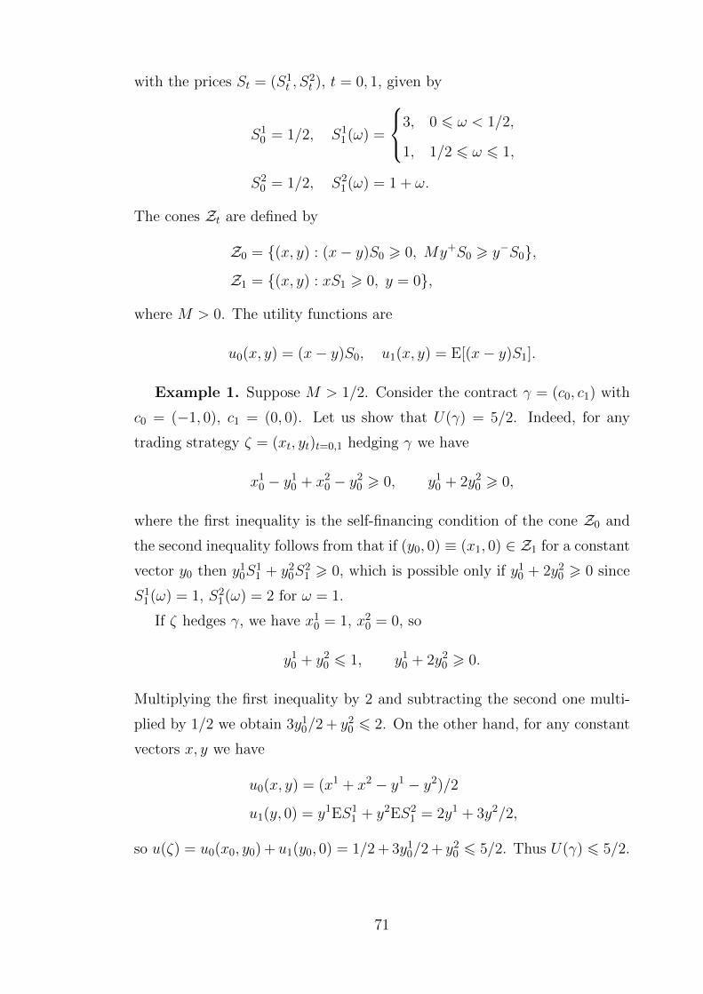
with the prices 𝑆𝑡 = (𝑆1𝑡 , 𝑆
2𝑡 ), 𝑡 = 0, 1, given by
𝑆10 = 1/2, 𝑆1
1(𝜔) =
⎧⎨⎩3, 0 6 𝜔 < 1/2,
1, 1/2 6 𝜔 6 1,
𝑆20 = 1/2, 𝑆2
1(𝜔) = 1 + 𝜔.
The cones 𝒵𝑡 are defined by
𝒵0 = {(𝑥, 𝑦) : (𝑥− 𝑦)𝑆0 > 0, 𝑀𝑦+𝑆0 > 𝑦−𝑆0},
𝒵1 = {(𝑥, 𝑦) : 𝑥𝑆1 > 0, 𝑦 = 0},
where 𝑀 > 0. The utility functions are
𝑢0(𝑥, 𝑦) = (𝑥− 𝑦)𝑆0, 𝑢1(𝑥, 𝑦) = E[(𝑥− 𝑦)𝑆1].
Example 1. Suppose 𝑀 > 1/2. Consider the contract 𝛾 = (𝑐0, 𝑐1) with
𝑐0 = (−1, 0), 𝑐1 = (0, 0). Let us show that 𝑈(𝛾) = 5/2. Indeed, for any
trading strategy 𝜁 = (𝑥𝑡, 𝑦𝑡)𝑡=0,1 hedging 𝛾 we have
𝑥10 − 𝑦10 + 𝑥20 − 𝑦20 > 0, 𝑦10 + 2𝑦20 > 0,
where the first inequality is the self-financing condition of the cone 𝒵0 and
the second inequality follows from that if (𝑦0, 0) ≡ (𝑥1, 0) ∈ 𝒵1 for a constant
vector 𝑦0 then 𝑦10𝑆11 + 𝑦20𝑆
21 > 0, which is possible only if 𝑦10 + 2𝑦20 > 0 since
𝑆11(𝜔) = 1, 𝑆2
1(𝜔) = 2 for 𝜔 = 1.
If 𝜁 hedges 𝛾, we have 𝑥10 = 1, 𝑥20 = 0, so
𝑦10 + 𝑦20 6 1, 𝑦10 + 2𝑦20 > 0.
Multiplying the first inequality by 2 and subtracting the second one multi-
plied by 1/2 we obtain 3𝑦10/2 + 𝑦20 6 2. On the other hand, for any constant
vectors 𝑥, 𝑦 we have
𝑢0(𝑥, 𝑦) = (𝑥1 + 𝑥2 − 𝑦1 − 𝑦2)/2
𝑢1(𝑦, 0) = 𝑦1E𝑆11 + 𝑦2E𝑆2
1 = 2𝑦1 + 3𝑦2/2,
so 𝑢(𝜁) = 𝑢0(𝑥0, 𝑦0) + 𝑢1(𝑦0, 0) = 1/2+ 3𝑦10/2+ 𝑦20 6 5/2. Thus 𝑈(𝛾) 6 5/2.
71

The value 5/2 is attained at the strategy with 𝑥0 = (1, 0), 𝑦0 = 𝑥1 = (2,−1),
𝑦1 = (0, 0), which hedges 𝛾 if 𝑀 > 1/2 as one can verify.
Suppose there exist supporting prices 𝑝0, 𝑝1 for the contract 𝛾. Then for
any (𝑥𝑡, 𝑦𝑡) ∈ 𝒵𝑡, 𝑡 = 0, 1, we have
5/2 = 𝑈(𝛾) > 𝑢0(𝑥0, 𝑦0) + 𝑢1(𝑥1, 𝑦1)− (𝑐0 + 𝑥0)𝑝0 + E[(𝑦0 − 𝑥1)𝑝1]. (2.10)
Take the following (𝑥𝑡, 𝑦𝑡):
𝑥0 = (1, 0), 𝑦0 = (2 + 𝜀,−1− 𝜀),
𝑥1 = (2 + 𝜀+ 𝑓𝜀,−1− 𝜀), 𝑦1 = (0, 0),
where 𝜀 ∈ (0, 2𝑀 − 1] is an arbitrary number and the function 𝑓𝜀 = 𝑓𝜀(𝜔)
is given by
𝑓𝜀(𝜔) = 𝜀 · I{𝜔 > 1/(1 + 𝜀)}
It is straightforward to check that (𝑥0, 𝑦0) ∈ 𝒵0 and (𝑥1, 𝑦1) ∈ 𝒵1.
Observe that 𝑢0(𝑥0, 𝑦0) = 0, 𝑢1(𝑥1, 𝑦1) = E[(2 + 𝜀+ 𝑓𝜀)𝑆11 − (1 + 𝜀)𝑆2
1 ] >
(2 + 𝜀)E𝑆11 − (1 + 𝜀)E𝑆1
2 = (2 + 𝜀) · 2 − (1 + 𝜀) · (3/2) = 5/2 + 𝜀/2, and
E(𝑦0 − 𝑥1)𝑝1 = −𝐸𝑓𝜀𝑝11, so from (2.10) we have
5/2 > 5/2 + 𝜀/2− E𝑓𝜀𝑝11.
However, since 𝑝1 ∈ 𝐿∞1 , there is a constant 𝑝 such that |𝑝11| 6 𝑝 a.s., so
−E𝑓𝜀𝑝1 > −𝑝E𝑓𝜀 = −𝑝𝜀2/(1 + 𝜀), i.e.
5/2 > 5/2 + 𝜀/2− 𝑝 · 𝜀2/(1 + 𝜀),
which is impossible for 𝜀 > 0 small enough. The contradiction means that
supporting prices do not exist.
Example 2. Let now 𝑀 > 0 be arbitrary (in particular, when 𝑀 = 0,
the markets forbids short sales). Consider the contracts 𝛾𝜀 = (𝑐0, 𝑐𝜀1) with
𝑐0 = (−2, 0), 𝑐𝜀1 = (0, 1 + 𝑓𝜀), where 𝜀 ∈ [0, 1/2] is an arbitrary number and
𝑓𝜀 is the function from Example 1.
Let us show that 𝑈(𝛾𝜀) = 5/2 − 𝜀 − E𝑓𝜀𝑆21 . Indeed, for any trading
72
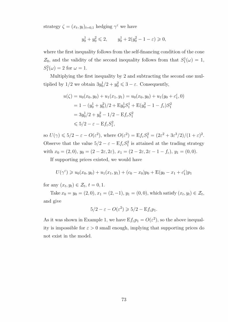
strategy 𝜁 = (𝑥𝑡, 𝑦𝑡)𝑡=0,1 hedging 𝛾𝜀 we have
𝑦10 + 𝑦20 6 2, 𝑦10 + 2(𝑦20 − 1− 𝜀) > 0,
where the first inequality follows from the self-financing condition of the cone
𝒵0, and the validity of the second inequality follows from that 𝑆11(𝜔) = 1,
𝑆21(𝜔) = 2 for 𝜔 = 1.
Multiplying the first inequality by 2 and subtracting the second one mul-
tiplied by 1/2 we obtain 3𝑦10/2 + 𝑦20 6 3− 𝜀. Consequently,
𝑢(𝜁) = 𝑢0(𝑥0, 𝑦0) + 𝑢1(𝑥1, 𝑦1) = 𝑢0(𝑥0, 𝑦0) + 𝑢1(𝑦0 + 𝑐𝜀1, 0)
= 1− (𝑦10 + 𝑦20)/2 + E𝑦10𝑆11 + E(𝑦20 − 1− 𝑓𝜀)𝑆
21
= 3𝑦10/2 + 𝑦20 − 1/2− E𝑓𝜀𝑆21
6 5/2− 𝜀− E𝑓𝜀𝑆21 ,
so 𝑈(𝛾) 6 5/2− 𝜀− 𝑂(𝜀2), where 𝑂(𝜀2) = E𝑓𝜀𝑆21 = (2𝜀2 + 3𝜀3/2)/(1 + 𝜀)2.
Observe that the value 5/2 − 𝜀 − E𝑓𝜀𝑆21 is attained at the trading strategy
with 𝑥0 = (2, 0), 𝑦0 = (2− 2𝜀, 2𝜀), 𝑥1 = (2− 2𝜀, 2𝜀− 1− 𝑓𝜀), 𝑦1 = (0, 0).
If supporting prices existed, we would have
𝑈(𝛾𝜀) > 𝑢0(𝑥0, 𝑦0) + 𝑢1(𝑥1, 𝑦1) + (𝑐0 − 𝑥0)𝑝0 + E(𝑦0 − 𝑥1 + 𝑐𝜀1)𝑝1
for any (𝑥𝑡, 𝑦𝑡) ∈ 𝒵𝑡, 𝑡 = 0, 1.
Take 𝑥0 = 𝑦0 = (2, 0), 𝑥1 = (2,−1), 𝑦1 = (0, 0), which satisfy (𝑥𝑡, 𝑦𝑡) ∈ 𝒵𝑡,
and give
5/2− 𝜀−𝑂(𝜀2) > 5/2− E𝑓𝜀𝑝1.
As it was shown in Example 1, we have E𝑓𝜀𝑝1 = 𝑂(𝜀2), so the above inequal-
ity is impossible for 𝜀 > 0 small enough, implying that supporting prices do
not exist in the model.
73

2.5 Appendix: geometric duality
Let 𝐿 be a normed linear space and 𝐿* its dual. Let 𝑓 be a real-valued
concave function defined on a convex set 𝑋 ⊂ 𝐿.
The steepness of 𝑓 from a point 𝑥 ∈ 𝑋 to a point 𝑥′ ∈ 𝑋, 𝑥′ = 𝑥, is
defined by
𝑠𝑥(𝑥′) =
𝑓(𝑥′)− 𝑓(𝑥)
‖𝑥′ − 𝑥‖.
An element 𝑝 ∈ 𝐿* is called a support of the function 𝑓 at a point 𝑥 ∈ 𝑋 if
𝑓(𝑥′)− 𝑓(𝑥) 6 𝑝 · (𝑥′ − 𝑥) for any 𝑥′ ∈ 𝑋.
The set of all supports of 𝑓 at 𝑥 is denoted by Σ𝑥 (which may be empty).
For a given 𝑥 ∈ 𝑋, consider the two problems:
(1) the primal problem:
find sup𝑥′∈𝑋∖{𝑥}
𝑠𝑥(𝑥′);
(2) the dual problem:
find inf𝑝∈Σ𝑥
‖𝑝‖.
The following theorem connects the primal and the dual problems and
plays an important role in many questions of convex analysis.
Proposition 2.1 (The Duality Theorem, [26]). The set Σ𝑥 is not empty
if and only if 𝑠𝑥(𝑥′) is bounded from above. In this case, if 𝑥 is not a point
where 𝑓 attains its global maximum, the values of the two problems are equal.
74

Chapter 3
Detection of changepoints in asset prices
In this chapter applications of sequential statistical methods to detecting
trend changes in asset prices are considered. We propose a model where one
holds an asset and wants to sell it before a fixed time 𝑇 . The price of the
asset initially increases but may start decreasing at an unknown moment of
time. The problem consists in detecting this change in the trend in order to
sell the asset for a high price.
The solution will be based on methods of changepoint (or disorder) de-
tection theory. The optimal moment of selling the asset will be represented
as the first moment of time when some statistic (the Shiryaev-Roberts statis-
tic or, equivalently, the posterior probability process), constructed from the
price sequence, exceeds a certain time-dependent threshold.
The mathematical theory of changepoint detection started developing in
1920-1950s in connection with problems of production quality control and
radiolocation (see a survey in [65]). Later it was also applied in the financial
context (see e. g. [62]). Changepoint detection methods can be divided into
the two groups: Bayesian and minimax methods. In the Bayesian setting, a
changepoint (a moment of disorder) is an unobservable random variable with
a known prior distribution, while in the minimax setting it is an unknown
parameter. In this chapter we follow the Bayesian approach.
The problem we consider was previously studied in [2, 14, 56] in the case
of continuous time when the evolution of an asset price is described by a
geometric Brownian motion, which changes its value of the drift coefficient at
an unknown moment of time (from a “favourable” value to an “unfavourable”
one). The result we obtain extends the results available in the literature to
the case of discrete time. Moreover, unlike the majority of previous results,
which assume the changepoint is exponentially distributed, we do not impose
75
any assumption on its prior distribution.
The first section of the chapter describes the model of asset prices with
changepoints. In Section 3.2 we introduce the basic statistics and formulate
the main theorem, which is proved in Section 3.3. Section 3.4 contains results
of numerical simulations.
3.1 The problem of selling an asset with a changepoint
We propose a model describing the price 𝑆 of an asset at moments of time
𝑡 = 0, 1, . . . , 𝑇 driven by a geometric Gaussian random walk with logarithmic
mean and variance (𝜇1, 𝜎1) up to an unknown moment of time 𝜃 and (𝜇2, 𝜎2)
after 𝜃. The moment 𝜃 will be interpreted as the point when the trend of the
asset changes from a favourable value to an unfavourable one, and is called
a changepoint (or a moment of disorder1).
Let 𝜉 = (𝜉𝑡)𝑇𝑡=1 be a sequence of i.i.d. (independent and identically dis-
tributed) standard normal random variables defined on a probability space
(Ω,F ,P) and let the sequence 𝑆 = (𝑆𝑡)𝑇𝑡=0 be defined by its logarithmic
increments as follows:
𝑆0 = 1, log𝑆𝑡
𝑆𝑡−1=
⎧⎨⎩𝜇1 + 𝜎1𝜉𝑡, 𝑡 < 𝜃,
𝜇2 + 𝜎2𝜉𝑡, 𝑡 > 𝜃,for 𝑡 = 1, 2, . . . , 𝑇,
where 𝜇1, 𝜇2 ∈ R, 𝜎1, 𝜎2 > 0 are known numbers, 𝜃 ∈ {1, 2, . . . , 𝑇 + 1} is an
unknown parameter. The equality 𝑆0 = 1 means that the prices are measured
relative to the price at time 𝑡 = 0 and does not reduce the generality of the
model.
We follow the Bayesian approach and assume that 𝜃 is a random variable
defined on (Ω,F ,P), independent of the sequence 𝜉𝑡 and taking values in
the set {1, 2, . . . , 𝑇 + 1} with known prior probabilities 𝑝𝑡 = P(𝜃 = 𝑡). The
value 𝑝1 is the probability that the changepoint appears from the beginning
1The term “disorder” comes from applications of the theory in production quality controlproblems, where 𝜃 can represent the moment of equipment breakage (a disorder) and increase ofdefective products.
76

of the sequence 𝑆𝑡 , and 𝑝𝑇+1 is the probability that the changepoint does
not appear within the time horizon [0, 𝑇 ]. The prior distribution function of
𝜃 is denoted by 𝐺(𝑡) =∑𝑢6𝑡
𝑝𝑢.
Let 𝑈𝛼 : R+ → R, 𝛼 6 1, be the family of functions defined as follows2:
𝑈𝛼(𝑥) = 𝛼𝑥𝛼 for 𝛼 = 0, 𝑈0(𝑥) = log 𝑥.
The problem considered in this chapter consists in finding the moment of
time 𝜏 which maximises the utility from selling the asset provided one holds
it at time 𝑡 = 0 and needs to sell it by 𝑡 = 𝑇 .
Let F = (F𝑡)𝑇𝑡=0, F𝑡 = 𝜎(𝑆𝑢; 𝑢 6 𝑡), be the filtration generated by the
price sequence 𝑆. By definition, a moment 𝜏 when one sells the asset should
be a stopping time of the filtration F, i. e. 𝜏 should be a random variable
taking values in the set {0, 1, . . . , 𝑇} such that {𝜔 : 𝜏(𝜔) 6 𝑡} ∈ F𝑡 for any
𝑡 = 0, . . . , 𝑇 . The class of all stopping times 𝜏 6 𝑇 of F is denoted by M.
The notion of a stopping time reflects the concept that a decision to sell the
asset at time 𝑡 should be based only on the information obtained from the
“historical” prices 𝑆0, 𝑆1, . . . , 𝑆𝑡 and should not rely on the “future” prices
𝑆𝑡+1, 𝑆𝑡+2, which are unknown at time 𝑡.
Mathematically, the problem of optimal selling of the asset with respect
to the utility function 𝑈𝛼 is formulated as the optimal stopping problem
𝑉𝛼 = sup𝜏∈M
E𝑈𝛼(𝑆𝜏 ). (3.1)
Its solution consists in finding the value 𝑉𝛼 and the optimal stopping time
𝜏 *𝛼, at which the supremum is attained (if such a stopping time exists).
It will be assumed that
𝜇1 > −𝛼𝜎21
2, 𝜇2 < −𝛼𝜎
22
2. (3.2)
In this case the sequence (𝑢𝛼𝑡 )𝑇𝑡=0, 𝑢
𝛼𝑡 = 𝑈𝛼(𝑆𝑡), is a submartingale3 when
2These functions are from capital growth theory and are known to maximize long run asymp-totic growth of wealth; see [5, 37, 40]. 𝑈0(𝑥) corresponds to the full Kelly strategy and 𝑈𝛼(𝑥),𝛼 < 0, correspond to fractional Kelly strategies blending cash with the optimal full Kelly portfolio.
3A random sequence (𝜁𝑡)𝑇𝑡=0 is called a submartingale (resp., a supermartingale or amartingale)
with respect to a filtration (F𝑡)𝑇𝑡=0 if E(𝜁𝑡 | F𝑡−1) > 𝜁𝑡−1 (resp., E(𝜁𝑡 | F𝑡−1) 6 𝜁𝑡−1 or
E(𝜁𝑡 | F𝑡−1) = 𝜁𝑡−1) for each 𝑡 = 1, . . . , 𝑇 .
77
the logarithmic returns of 𝑆 are i.i.d. N (𝜇1, 𝜎21) random variables, and
a supermartingale when they are i.i.d. N (𝜇2, 𝜎22) random variables. In
the former case, the value of 𝑢𝑡 increases on average as 𝑡 increases, so it
is profitable to hold the asset, and in the latter case the average value of
𝑢𝑡 decreases meaning that one needs to sell the asset as soon as possible.
Consequently, the random variable 𝜃 represents the moment of time when
holding the asset becomes unprofitable. Note that 𝜃 is not measurable with
respect to F𝑡 (except the trivial case when 𝜃 is a constant random variable),
which can be interpreted as the unobservability of the changepoint.
It is also reasonable to assume that 𝑝1 > 0 — otherwise it is clear that
one should never stop at time 𝑡 = 0 (i. e. the optimal stopping time 𝜏 *𝛼 > 1),
and the problem can be reduced to the smaller time horizon 𝑡 = 1, 2, . . . , 𝑇 .
Nevertheless, the result of the main theorem in the next section will be still
valid if 𝑝1 = 0.
3.2 The structure of optimal selling times
In order to formulate the main result of the chapter, introduce auxiliary
notation. Let 𝑋 = (𝑋𝑡)𝑇𝑡=1 denote the logarithmic returns of the prices:
𝑋𝑡 = log𝑆𝑡
𝑆𝑡−1, 𝑡 = 1, . . . , 𝑇.
On the space (Ω,F𝑇 ) introduce the family of probability measures P𝑢,
𝑢 = 1, . . . , 𝑇+1, generated by the sequence 𝑆 with the value of the parameter
𝜃 ≡ 𝑢. Following the standard notation of the changepoint detection theory,
let4 P∞ ≡ P𝑇+1, and denote by P𝑡 = P | F𝑡, P𝑢𝑡 = P𝑢 | F𝑡 the restrictions
of the corresponding measures to the 𝜎-algebra F𝑡.
4Typically, P∞ denotes the measure when there is no change in the probability law of theobservable sequence on the whole time horizon (i. e. the change “occurs” at time 𝑡 = ∞). Sincein the problem considered the time horizon is finite, this measure has the same meaning as P𝑇+1.
78
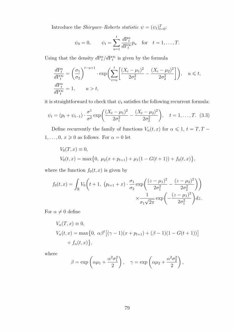
Introduce the Shiryaev–Roberts statistic 𝜓 = (𝜓𝑡)𝑇𝑡=0:
𝜓0 = 0, 𝜓𝑡 =𝑡∑
𝑢=1
𝑑P𝑢𝑡
𝑑P∞𝑡
𝑝𝑢 for 𝑡 = 1, . . . , 𝑇.
Using that the density 𝑑P𝑢𝑡 /𝑑P
∞𝑡 is given by the formula
𝑑P𝑢𝑡
𝑑P∞𝑡
=
(𝜎1𝜎2
)𝑡−𝑢+1
· exp( 𝑡∑
𝑖=𝑢
[(𝑋𝑖 − 𝜇1)
2
2𝜎21− (𝑋𝑖 − 𝜇2)
2
2𝜎22
]), 𝑢 6 𝑡,
𝑑P𝑢𝑡
𝑑P∞𝑡
= 1, 𝑢 > 𝑡,
it is straightforward to check that 𝜓𝑡 satisfies the following recurrent formula:
𝜓𝑡 = (𝑝𝑡 + 𝜓𝑡−1) ·𝜎1
𝜎2exp
((𝑋𝑡 − 𝜇1)
2
2𝜎21− (𝑋𝑡 − 𝜇2)
2
2𝜎22
), 𝑡 = 1, . . . , 𝑇. (3.3)
Define recurrently the family of functions 𝑉𝛼(𝑡, 𝑥) for 𝛼 6 1, 𝑡 = 𝑇, 𝑇 −1, . . . , 0, 𝑥 > 0 as follows. For 𝛼 = 0 let
𝑉0(𝑇, 𝑥) ≡ 0,
𝑉0(𝑡, 𝑥) = max{0, 𝜇2(𝑥+ 𝑝𝑡+1) + 𝜇1(1−𝐺(𝑡+ 1)) + 𝑓0(𝑡, 𝑥)
},
where the function 𝑓0(𝑡, 𝑥) is given by
𝑓0(𝑡, 𝑥) =
∫R𝑉0
(𝑡+ 1,
(𝑝𝑡+1 + 𝑥) · 𝜎1
𝜎2exp
((𝑧 − 𝜇1)
2
2𝜎21− (𝑧 − 𝜇2)
2
2𝜎22
))× 1
𝜎1√2𝜋
exp
(−(𝑧 − 𝜇1)
2
2𝜎21
)𝑑𝑧.
For 𝛼 = 0 define
𝑉𝛼(𝑇, 𝑥) ≡ 0,
𝑉𝛼(𝑡, 𝑥) = max{0, 𝛼𝛽𝑡
[(𝛾 − 1)(𝑥+ 𝑝𝑡+1) + (𝛽 − 1)(1−𝐺(𝑡+ 1))
]+ 𝑓𝛼(𝑡, 𝑥)
},
where
𝛽 = exp
(𝛼𝜇1 +
𝛼2𝜎212
), 𝛾 = exp
(𝛼𝜇2 +
𝛼2𝜎222
),
79
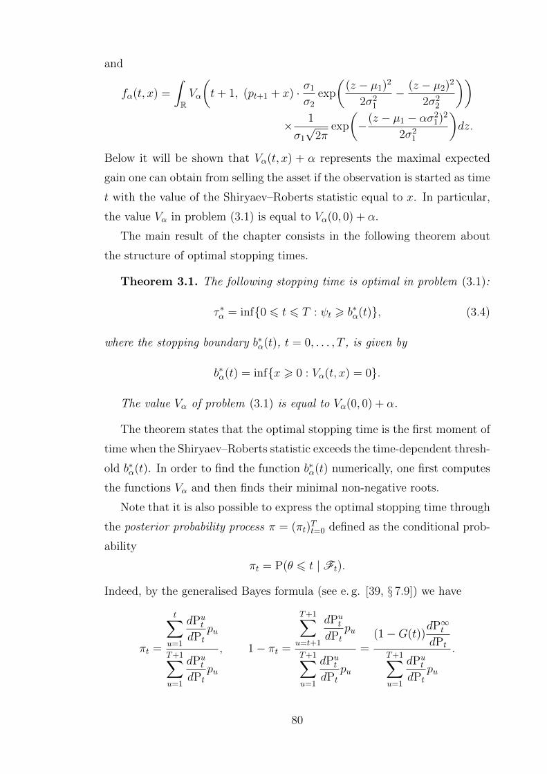
and
𝑓𝛼(𝑡, 𝑥) =
∫R𝑉𝛼
(𝑡+ 1, (𝑝𝑡+1 + 𝑥) · 𝜎1
𝜎2exp
((𝑧 − 𝜇1)
2
2𝜎21− (𝑧 − 𝜇2)
2
2𝜎22
))× 1
𝜎1√2𝜋
exp
(−(𝑧 − 𝜇1 − 𝛼𝜎21)
2
2𝜎21
)𝑑𝑧.
Below it will be shown that 𝑉𝛼(𝑡, 𝑥) + 𝛼 represents the maximal expected
gain one can obtain from selling the asset if the observation is started as time
𝑡 with the value of the Shiryaev–Roberts statistic equal to 𝑥. In particular,
the value 𝑉𝛼 in problem (3.1) is equal to 𝑉𝛼(0, 0) + 𝛼.
The main result of the chapter consists in the following theorem about
the structure of optimal stopping times.
Theorem 3.1. The following stopping time is optimal in problem (3.1):
𝜏 *𝛼 = inf{0 6 𝑡 6 𝑇 : 𝜓𝑡 > 𝑏*𝛼(𝑡)}, (3.4)
where the stopping boundary 𝑏*𝛼(𝑡), 𝑡 = 0, . . . , 𝑇 , is given by
𝑏*𝛼(𝑡) = inf{𝑥 > 0 : 𝑉𝛼(𝑡, 𝑥) = 0}.
The value 𝑉𝛼 of problem (3.1) is equal to 𝑉𝛼(0, 0) + 𝛼.
The theorem states that the optimal stopping time is the first moment of
time when the Shiryaev–Roberts statistic exceeds the time-dependent thresh-
old 𝑏*𝛼(𝑡). In order to find the function 𝑏*𝛼(𝑡) numerically, one first computes
the functions 𝑉𝛼 and then finds their minimal non-negative roots.
Note that it is also possible to express the optimal stopping time through
the posterior probability process 𝜋 = (𝜋𝑡)𝑇𝑡=0 defined as the conditional prob-
ability
𝜋𝑡 = P(𝜃 6 𝑡 | F𝑡).
Indeed, by the generalised Bayes formula (see e. g. [39, S 7.9]) we have
𝜋𝑡 =
𝑡∑𝑢=1
𝑑P𝑢𝑡
𝑑P𝑡𝑝𝑢
𝑇+1∑𝑢=1
𝑑P𝑢𝑡
𝑑P𝑡𝑝𝑢
, 1− 𝜋𝑡 =
𝑇+1∑𝑢=𝑡+1
𝑑P𝑢𝑡
𝑑P𝑡𝑝𝑢
𝑇+1∑𝑢=1
𝑑P𝑢𝑡
𝑑P𝑡𝑝𝑢
=(1−𝐺(𝑡))
𝑑P∞𝑡
𝑑P𝑡𝑇+1∑𝑢=1
𝑑P𝑢𝑡
𝑑P𝑡𝑝𝑢
.
80

This implies
𝜓𝑡 =𝜋𝑡
1− 𝜋𝑡(1−𝐺(𝑡)), 𝜋𝑡 =
𝜓𝑡
𝜓𝑡 + 1−𝐺(𝑡).
Consequently, the optimal stopping time in problem (3.1) can be equivalently
represented in the form
𝜏 *𝛼 = inf{0 6 𝑡 6 𝑇 : 𝜋𝑡 > 𝑏*𝛼(𝑡)}, where 𝑏*𝛼(𝑡) = 𝑏*𝛼(𝑡)
𝑏*𝛼(𝑡) + 1−𝐺(𝑡).
This representation provides a clear interpretation of the optimal stopping
time: one should sell the asset as soon as she becomes sufficiently confident
that the disorder has already happened, which quantitatively means that the
posterior probability 𝜋𝑡 exceeds the threshold 𝑏*𝛼(𝑡).
3.3 The proof of the main theorem
The proof of the theorem will be given in two steps. First, problem (3.1)
will be reduced to an optimal stopping problem for the Shiryaev–Roberts
statistic 𝜓 with respect to a new probability measure on (Ω,F𝑇 ). Then we
show that 𝜓𝑡 is a Markov sequence with respect to this measure and apply
methods of Markovian optimal stopping theory to the problem.
Step 1. On the measure space (Ω, F𝑇 ) introduce the family of probability
measures Q𝛼, 𝛼 6 1, such that the logarithmic returns 𝑋𝑡, 𝑡 = 1, . . . , 𝑇 , are
i.i.d 𝒩 (𝜇1 + 𝛼𝜎21, 𝜎21) random variables under Q𝛼. In particular, Q0 ≡ P∞.
For 𝑡 = 1, . . . , 𝑇 , the explicit formula for the density 𝑑P𝑡/𝑑Q𝛼𝑡 , where Q𝛼
𝑡 =
Q𝛼 | F𝑡, is given by the formula
𝑑P𝑡
𝑑Q𝛼𝑡
=𝑑P𝑡
𝑑Q0𝑡
· 𝑑Q0𝑡
𝑑Q𝛼𝑡
=
(𝑇+1∑𝑢=1
𝑑P𝑢𝑡
𝑑P∞𝑡
𝑝𝑢
)· 𝑑Q
0𝑡
𝑑Q𝛼𝑡
=
( 𝑡∑𝑢=1
𝑑P𝑢𝑡
𝑑P∞𝑡
𝑝𝑢 +𝑇+1∑
𝑢=𝑡+1
𝑝𝑢
)· exp
(𝛼𝜇1𝑡+
𝛼2𝜎212
𝑡− 𝛼
𝑡∑𝑢=1
𝑋𝑖
)
= (𝜓𝑡 + 1−𝐺(𝑡))𝛽𝑡 · exp(−𝛼
𝑡∑𝑢=1
𝑋𝑖
).
81

We show that for any stopping time 𝜏 ∈ M it holds that
E𝑈0(𝑆𝜏 ) = EQ0
[ 𝜏∑𝑡=1
[𝜇2𝜓𝑡 + 𝜇1(1−𝐺(𝑡))
]], (3.5)
E𝑈𝛼(𝑆𝜏 ) = 𝛼EQ𝛼
[ 𝜏∑𝑡=1
𝛽𝑡−1[(𝛽 − 𝛽/𝛾)𝜓𝑡 + (𝛽 − 1)(1−𝐺(𝑡))
]]+ 𝛼 for 𝛼 = 0,
(3.6)
where EQ𝛼
denotes the expectation with respect to Q𝛼. Here and below, we
define𝜏∑
𝑡=1[. . .] = 0 if 𝜏 = 0.
In order to prove (3.5), observe that
E𝑈0(𝑆𝜏 ) = E𝜏∑
𝑡=1
𝑋𝑡 = EQ0
[𝑑P𝜏
𝑑Q0𝜏
𝜏∑𝑡=1
𝑋𝑡
]= EQ0
[(𝜓𝜏 + 1−𝐺(𝜏))
𝜏∑𝑡=1
𝑋𝑡
].
Using the “discrete version” of the integration by parts formula,
𝑎𝑡𝑏𝑡 =𝑡∑
𝑠=1
𝑎𝑠Δ𝑏𝑠 +𝑡∑
𝑠=1
𝑏𝑠−1Δ𝑎𝑠 + 𝑎0𝑏0, (3.7)
valid for any sequences 𝑎𝑡 and 𝑏𝑡 with the notation Δ𝑎𝑠 = 𝑎𝑠 − 𝑎𝑠−1, Δ𝑏𝑠 =
𝑏𝑠 − 𝑏𝑠−1, we obtain
E𝑈0(𝑆𝜏 ) = EQ0
[ 𝜏∑𝑡=1
(𝜓𝑡 + 1−𝐺(𝑡))𝑋𝑡 +𝜏∑
𝑡=1
𝑡−1∑𝑠=1
𝑋𝑠(𝜓𝑡 − 𝜓𝑡−1 − 𝑝𝑡)
]. (3.8)
The sequence 𝜓𝑡 + 1 − 𝐺(𝑡) is a martingale with respect to the measure
Q0 since it is the sequence of the densities 𝑑P𝑡/𝑑Q0𝑡 . This implies that the
expectation of the second sum in the above formula is zero. Indeed, we have
EQ0
[ 𝜏∑𝑡=1
𝑡−1∑𝑠=1
𝑋𝑠(𝜓𝑡 − 𝜓𝑡−1 − 𝑝𝑡)
]
= EQ0
[𝑇+1∑𝑡=1
𝑡−1∑𝑠=1
EQ0[𝑋𝑠(𝜓𝑡 − 𝜓𝑡−1 − 𝑝𝑡)I(𝑡 6 𝜏) | F𝑡−1
]]= 0,
where we use that 𝑋𝑠 and I(𝑡 6 𝜏) are F𝑡−1-measurable random variables,
82

so they can be taken out of the conditional expectation, and
EQ0
(𝜓𝑡 − 𝜓𝑡−1 − 𝑝𝑡 | F𝑡−1) = 0, 𝑡 = 1, . . . , 𝑇,
as follows from that 𝜓𝑡 + 1−𝐺(𝑡) is a martingale.
For the first sum in (3.8) we have
EQ0
[ 𝜏∑𝑡=1
(𝜓𝑡 + 1−𝐺(𝑡))𝑋𝑡
]
= EQ0
[𝑇+1∑𝑡=1
EQ0((𝜓𝑡 + 1−𝐺(𝑡))𝑋𝑡I(𝑡 6 𝜏) | F𝑡−1
)]= EQ0
[ 𝜏∑𝑡=1
[EQ0
(𝑝𝑡 + 𝜓𝑡−1)𝜇2 + 𝜇1(1−𝐺(𝑡))]]
= EQ0
[ 𝜏∑𝑡=1
[𝜇2𝜓𝑡 + 𝜇1(1−𝐺(𝑡))]
].
In the second equality we use that I(𝑡 6 𝜏) is an F𝑡−1-measurable random
variable and it can be taken out of the conditional expectation, 𝑋𝑡 is indepen-
dent of F𝑡−1, so EQ0
[(1−𝐺(𝑡))𝑋𝑡 | F𝑡−1] = (1−𝐺(𝑡))EQ0
𝑋𝑡 = (1−𝐺(𝑡))𝜇1,and, as follows from (3.3),
EQ0
(𝜓𝑡𝑋𝑡 | F𝑡−1) = (𝑝𝑡 + 𝜓𝑡−1)𝜎1𝜎2
EQ0
[𝑋𝑡 exp
((𝑋𝑡 − 𝜇1)
2
2𝜎21− (𝑋𝑡 − 𝜇2)
2
2𝜎22
)]= (𝑝𝑡 + 𝜓𝑡−1)𝜇2.
In the third equality we use the representation
EQ0
[ 𝜏∑𝑡=1
(𝑝𝑡 + 𝜓𝑡−1)
]= EQ0
[𝑇+1∑𝑡=1
EQ0(𝜓𝑡 | F𝑡−1
)I(𝑡 6 𝜏)
]
= EQ0
[𝑇+1∑𝑡=1
EQ0(𝜓𝑡I(𝑡 6 𝜏) | F𝑡−1
)]= EQ0
[ 𝜏∑𝑡=1
𝜓𝑡
].
This proves formula (3.5).
83

Let us prove (3.6). We have
E𝑈𝛼(𝑆𝜏 ) = 𝛼E exp
(𝛼
𝜏∑𝑡=1
𝑋𝑡
)= 𝛼EQ𝛼
[𝑑P𝜏
𝑑Q𝛼𝜏
exp
(𝛼
𝜏∑𝑡=1
𝑋𝑡
)]= 𝛼EQ𝛼[
(𝜓𝜏 + 1−𝐺(𝜏))𝛽𝜏]
= 𝛼EQ𝛼
[ 𝜏∑𝑡=1
[(𝜓𝑡 + 1−𝐺(𝑡))(𝛽𝑡 − 𝛽𝑡−1) + 𝛽𝑡−1(𝜓𝑡 − 𝜓𝑡−1 − 𝑝𝑡)
]]+ 𝛼,
where in the third equality we use the formula for the conditional density
𝑑P𝑡/𝑑Q𝛼𝑡 , and in the last equality we use formula (3.7). Using representation
(3.3), it is possible to verify the following expression for the conditional
expectation EQ𝛼
(𝜓𝑡 | F𝑡−1):
EQ𝛼
(𝜓𝑡 | F𝑡−1) =𝛾
𝛽(𝜓𝑡−1 + 𝑝𝑡) for 𝑡 = 1, . . . , 𝑇. (3.9)
To check that the right-hand side (𝑅𝐻) of above expression for E𝑈𝛼(𝑆𝜏 ) co-
incides with the right-hand side (𝑅𝐻) of (3.6), we show that their difference
is equal to zero:
(𝑅𝐻)− (𝑅𝐻) = 𝛼EQ𝛼
[ 𝜏∑𝑡=1
𝛽𝑡−1(𝜓𝑡𝛽/𝛾 − 𝜓𝑡−1 − 𝑝𝑡)
]
= 𝛼EQ𝛼
[𝑇+1∑𝑡=1
𝛽𝑡−1(𝜓𝑡𝛽/𝛾 − 𝜓𝑡−1 − 𝑝𝑡)I(𝑡 6 𝜏)
]
= 𝛼EQ𝛼
[𝑇+1∑𝑡=1
EQ𝛼[𝛽𝑡−1(𝜓𝑡𝛽/𝛾 − 𝜓𝑡−1 − 𝑝𝑡)I(𝑡 6 𝜏) | F𝑡−1
]]
= 𝛼EQ𝛼
[𝑇+1∑𝑡=1
𝛽𝑡−1(EQ𝛼
(𝜓𝑡 | F𝑡−1)𝛽/𝛾 − 𝜓𝑡−1 − 𝑝𝑡)I(𝑡 6 𝜏)
]= 0,
where in the fourth equality we use that 𝜓𝑡−1 and I(𝑡 6 𝜏) are F𝑡−1-
measurable random variables, so their conditional expectations coincides
with themselves, and apply (3.9). This proves (3.6).
Step 2. For convenience of further notation, let 𝐹𝛼(𝑡, 𝜓) denote the terms
in the sums in (3.5)–(3.6):
𝐹0(𝑡, 𝑥) = 𝜇2𝑥+ 𝜇1(1−𝐺(𝑡)),
𝐹𝛼(𝑡, 𝑥) = 𝛼𝛽𝑡−1[(𝛽 − 𝛽/𝛾)𝑥+ (𝛽 − 1)(1−𝐺(𝑡))].(3.10)
84

Representations (3.5)–(3.6) allow to reduce problem (3.1) to the optimal
stopping problems for the Shiryaev–Roberts statistic 𝜓
𝑉𝛼 = sup𝜏∈M
EQ𝛼
[𝜏∑
𝑢=1
𝐹𝛼(𝑢, 𝜓𝑢)
]+ 𝛼,
so that the optimal stopping times in these problems will be also optimal in
problem (3.1).
Let M𝑡 denote the class of all stopping times 𝜏 of the filtration F such
that 𝜏 6 𝑡. In particular, M𝑇 = M.
According to the results of [64, Ch. II, S 2.15], the Shiryaev–Roberts statis-tic is a Markov sequence with respect to the filtration F under each measure
Q𝛼, 𝛼 6 1, since 𝜓𝑡 is a function of 𝜓𝑡−1 and 𝑋𝑡, while 𝑋𝑡 form a sequence
of independent random variables. Following the general theory of optimal
stopping of Markov sequences (see e. g. [47, Ch. I]), introduce the family of
the value functions 𝑉𝛼(𝑡, 𝑥) for 𝑡 ∈ {0, 1, . . . , 𝑇}, 𝑥 > 0:
𝑉𝛼(𝑡, 𝑥) = sup𝜏∈M𝑇−𝑡
EQ𝛼
[𝜏∑
𝑢=1
𝐹𝛼(𝑡+ 𝑢, 𝜓𝑢(𝑡, 𝑥))
], (3.11)
where 𝜓(𝑡, 𝑥) = (𝜓𝑢(𝑡, 𝑥))𝑇−𝑡𝑢=0 is a sequence of random variables defined by
the recurrent formula
𝜓0(𝑡, 𝑥) = 𝑥,
𝜓𝑢(𝑡, 𝑥) = (𝑝𝑡+𝑢 + 𝜓𝑢−1(𝑡, 𝑥)) ·𝜎1𝜎2
exp
((𝑋𝑢 − 𝜇1)
2
2𝜎21− (𝑋𝑢 − 𝜇2)
2
2𝜎22
)with 𝑋1, 𝑋2, . . . being i.i.d. 𝒩 (𝜇1 + 𝛼𝜎21, 𝜎
21) random variables with respect
to the measure Q𝛼. The sums in the definition of 𝑉𝛼(𝑡, 𝑥) are equal to zero
if 𝜏 = 0, which, in particular, means that 𝑉𝛼(𝑇, 𝑥) = 0 for any 𝑥 > 0.
The functions 𝑉𝛼(𝑡, 𝑥) represent the maximal possible gain in the optimal
stopping problem if the observation starts at time 𝑡 with the value of the
Shiryaev–Roberts statistic 𝑥. From formulae (3.5)–(3.6), it follows that orig-
inal problem (3.1) corresponds to 𝑡 = 0, 𝑥 = 0, so the optimal stopping time
for 𝑉𝛼(0, 0) will be the optimal stopping time in (3.1), and 𝑉𝛼 = 𝑉𝛼(0, 0)+𝑎.
The well-known result of the optimal stopping theory for Markov se-
85
quences (see [47, Theorem 1.8]) states that the value functions 𝑉𝛼(𝑡, 𝑥) satisfy
the following Wald–Bellman equations for 𝑡 = 0, . . . , 𝑇 − 1:
𝑉𝛼(𝑡, 𝑥) = max{0, EQ𝛼
[𝐹𝛼(𝑡+ 1, 𝜓1(𝑡, 𝑥)) + 𝑉𝛼(𝑡+ 1, 𝜓1(𝑡, 𝑥))]}. (3.12)
Here, 0 is the gain from instantaneous stopping in the problems at hand.
Using that 𝑋𝑡 are i.i.d N (𝜇1+𝛼𝜎21, 𝜎
21) random variables with respect to Q𝛼
and computing the expectations EQ𝛼
[. . . .] in the above equation, we obtain
that the functions 𝑉𝛼(𝑡, 𝑥) satisfy the recurrent relations on p. 79.
From [47, Theorem 1.7] it follows that the optimal stopping time in prob-
lem (3.1) is the first moment of time when 𝜓𝑡 enters the stopping set 𝐷𝛼:
𝐷𝛼 = {(𝑡, 𝑥) : 𝑉𝛼(𝑡, 𝑥) = 0}, 𝜏 *𝛼 = inf{𝑡 > 0 : (𝑡, 𝜓𝑡) ∈ 𝐷𝛼}.
In order to prove representation (3.4), we show that for fixed 𝑡 and 𝛼, the
function 𝑥 ↦→ 𝑉𝛼(𝑡, 𝑥) is continuous and non-increasing, and there exists 𝑥
such that 𝑉𝛼(𝑡, 𝑥) = 0. The non-increasing follows from that 𝜓𝑢(𝑡, 𝑥1) >
𝜓𝑢(𝑡, 𝑥2) whenever 𝑥1 > 𝑥2, and the coefficients 𝜇2 and 𝛼𝛽𝑡(1 − 1/𝛾) are
negative in the formulae for 𝐹0(𝑡, 𝑥) and 𝐹𝛼(𝑡, 𝑥) respectively as follows from
the assumption 𝜇2 < −𝛼𝜎22/2 (see (3.2)).
In order to prove the continuity of 𝑥 ↦→ 𝑉𝛼(𝑡, 𝑥), we show by induction
over 𝑡 = 𝑇, 𝑇 − 1, . . . , 0 that for arbitrary 0 6 𝑥1 6 𝑥2 it holds that
𝑉𝛼(𝑡, 𝑥1)− 𝑉𝛼(𝑡, 𝑥2) 6 𝑐𝛼𝑡 (𝑥2 − 𝑥1) (3.13)
with the constants
𝑐𝛼𝑡 =
⎧⎨⎩|𝜇2|(𝑇 − 𝑡), 𝛼 = 0
𝛼𝛽𝑡(1− 𝛾𝑇−𝑡), 𝛼 = 0.
For 𝑡 = 𝑇 the claim is valid, because 𝑉𝛼(𝑇, 𝑥) = 0 for all 𝑥 > 0. Suppose it
holds for some 𝑡 = 𝑠 and consider 𝑡 = 𝑠 − 1. From the formulae on p. 79 it
86

follows that
𝑉𝛼(𝑠− 1, 𝑥1)− 𝑉𝛼(𝑠− 1, 𝑥2)
6
⎧⎨⎩|𝜇2|(𝑥2 − 𝑥1) + 𝑓0(𝑠− 1, 𝑥1)− 𝑓0(𝑠− 1, 𝑥2), 𝛼 = 0,
𝛼𝛽𝑠−1(1− 𝛾)(𝑥2 − 𝑥1) + 𝑓𝛼(𝑠− 1, 𝑥1)− 𝑓𝛼(𝑠− 1, 𝑥2), 𝛼 = 0.
Further, using the induction assumption for 𝑡 = 𝑠, we find
𝑓𝛼(𝑠− 1, 𝑥1)− 𝑓𝛼(𝑠− 1, 𝑥2) 6∫R
𝑐𝛼𝑠 (𝑥2 − 𝑥1)
𝜎2√2𝜋
exp
((𝑧 − 𝜇1)
2
2𝜎21− (𝑧 − 𝜇2)
2
2𝜎22
)× exp
((𝑧 − 𝜇1 − 𝛼𝜎21)
2
2𝜎21
)𝑑𝑧 = 𝑐𝛼𝑠 (𝑥2 − 𝑥1)
𝛾
𝛽.
Combining it with the previous inequality we find for 𝛼 = 0
𝑉𝛼(𝑠− 1, 𝑥1)− 𝑉𝛼(𝑠− 1, 𝑥2) 6 (𝑥2 − 𝑥1)(|𝜇2|+ 𝑐𝛼𝑠 ) = 𝑐𝛼𝑠−1(𝑥2 − 𝑥1)
and for 𝛼 = 0
𝑉𝛼(𝑠− 1, 𝑥1)− 𝑉𝛼(𝑠− 1, 𝑥2) 6 (𝑥2 − 𝑥1)(𝛼𝛽𝑠−1(1− 𝛾) + 𝑐𝛼𝑠 𝛾/𝛽)
= 𝑐𝛼𝑠−1(𝑥2 − 𝑥1),
which proves the claim. Since 0 6 𝑉𝛼(𝑡, 𝑥1)− 𝑉𝛼(𝑡, 𝑥2) because 𝑥 ↦→ 𝑉𝛼(𝑡, 𝑥)
is a non-increasing function, we obtain that it is continuous.
Finally by induction over 𝑡 = 𝑇, 𝑇 − 1, . . . , 0 we prove that there exists a
root 𝑟𝛼,𝑡 of the function 𝑥 ↦→ 𝑉𝛼(𝑡, 𝑥). For 𝑡 = 𝑇 this is true since 𝑉𝛼(𝑇, 𝑥) = 0
for all 𝑥 > 0. Suppose there exists a root for 𝑡 = 𝑠 > 0. Then for 𝑡 = 𝑠− 1
and 𝑥→ +∞ we have
EQ𝛼
𝑉𝛼(𝑠, 𝜓1(𝑠− 1, 𝑥)) 6 sup06𝑦6𝑟𝛼,𝑠
𝑉𝛼(𝑠, 𝑦) ·Q𝛼{𝜓1(𝑠− 1, 𝑥) 6 𝑟𝛼,𝑠} → 0
since 𝑦 ↦→ 𝑉𝛼(𝑠, 𝑦) is a continuous function and, hence, bounded on the
segment [0, 𝑟𝛼,𝑠], while Q𝛼{𝜓1(𝑠 − 1, 𝑥) 6 𝑟𝛼,𝑠} → 0 for 𝑥 → +∞ as follows
from the definition of 𝜓1(𝑡, 𝑥). On the other hand, 𝐹𝛼(𝑠 − 1, 𝑥) → −∞as 𝑥 → +∞, which follows from that, according to the assumption 𝜇2 <
−𝛼𝜎22/2 (see (3.2)), the coefficients 𝜇2 or 𝛼𝛽𝑡−1(𝛽 − 𝛽/𝛾) in front of 𝑥 in
formula (3.10) are negative respectively in the case 𝛼 = 0 or 𝛼 = 0. Then
87
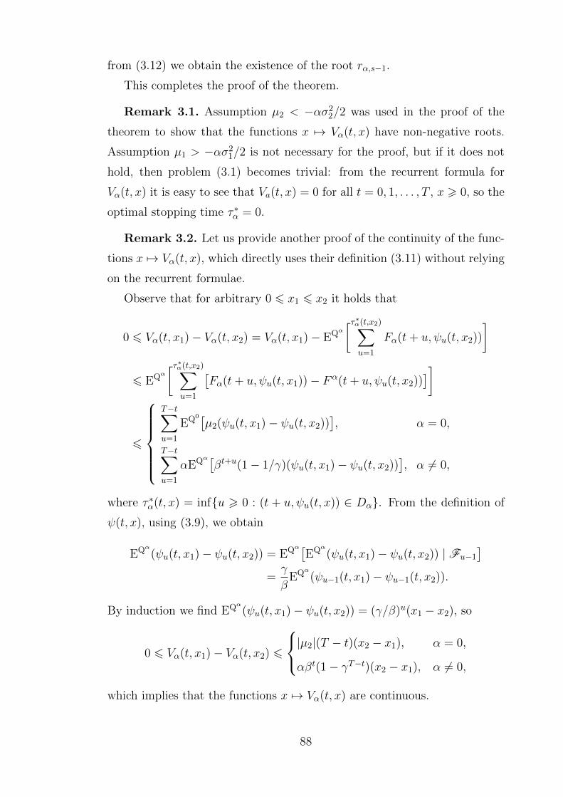
from (3.12) we obtain the existence of the root 𝑟𝛼,𝑠−1.
This completes the proof of the theorem.
Remark 3.1. Assumption 𝜇2 < −𝛼𝜎22/2 was used in the proof of the
theorem to show that the functions 𝑥 ↦→ 𝑉𝛼(𝑡, 𝑥) have non-negative roots.
Assumption 𝜇1 > −𝛼𝜎21/2 is not necessary for the proof, but if it does not
hold, then problem (3.1) becomes trivial: from the recurrent formula for
𝑉𝛼(𝑡, 𝑥) it is easy to see that 𝑉𝑎(𝑡, 𝑥) = 0 for all 𝑡 = 0, 1, . . . , 𝑇 , 𝑥 > 0, so the
optimal stopping time 𝜏 *𝛼 = 0.
Remark 3.2. Let us provide another proof of the continuity of the func-
tions 𝑥 ↦→ 𝑉𝛼(𝑡, 𝑥), which directly uses their definition (3.11) without relying
on the recurrent formulae.
Observe that for arbitrary 0 6 𝑥1 6 𝑥2 it holds that
0 6 𝑉𝛼(𝑡, 𝑥1)− 𝑉𝛼(𝑡, 𝑥2) = 𝑉𝛼(𝑡, 𝑥1)− EQ𝛼
[𝜏*𝛼(𝑡,𝑥2)∑𝑢=1
𝐹𝛼(𝑡+ 𝑢, 𝜓𝑢(𝑡, 𝑥2))
]
6 EQ𝛼
[𝜏*𝛼(𝑡,𝑥2)∑𝑢=1
[𝐹𝛼(𝑡+ 𝑢, 𝜓𝑢(𝑡, 𝑥1))− 𝐹𝛼(𝑡+ 𝑢, 𝜓𝑢(𝑡, 𝑥2))
]]
6
⎧⎪⎪⎪⎪⎪⎨⎪⎪⎪⎪⎪⎩
𝑇−𝑡∑𝑢=1
EQ0[𝜇2(𝜓𝑢(𝑡, 𝑥1)− 𝜓𝑢(𝑡, 𝑥2))
], 𝛼 = 0,
𝑇−𝑡∑𝑢=1
𝛼EQ𝛼[𝛽𝑡+𝑢(1− 1/𝛾)(𝜓𝑢(𝑡, 𝑥1)− 𝜓𝑢(𝑡, 𝑥2))
], 𝛼 = 0,
where 𝜏 *𝛼(𝑡, 𝑥) = inf{𝑢 > 0 : (𝑡 + 𝑢, 𝜓𝑢(𝑡, 𝑥)) ∈ 𝐷𝛼}. From the definition of
𝜓(𝑡, 𝑥), using (3.9), we obtain
EQ𝛼
(𝜓𝑢(𝑡, 𝑥1)− 𝜓𝑢(𝑡, 𝑥2)) = EQ𝛼[EQ𝛼
(𝜓𝑢(𝑡, 𝑥1)− 𝜓𝑢(𝑡, 𝑥2)) | F𝑢−1
]=𝛾
𝛽EQ𝛼
(𝜓𝑢−1(𝑡, 𝑥1)− 𝜓𝑢−1(𝑡, 𝑥2)).
By induction we find EQ𝛼
(𝜓𝑢(𝑡, 𝑥1)− 𝜓𝑢(𝑡, 𝑥2)) = (𝛾/𝛽)𝑢(𝑥1 − 𝑥2), so
0 6 𝑉𝛼(𝑡, 𝑥1)− 𝑉𝛼(𝑡, 𝑥2) 6
⎧⎨⎩|𝜇2|(𝑇 − 𝑡)(𝑥2 − 𝑥1), 𝛼 = 0,
𝛼𝛽𝑡(1− 𝛾𝑇−𝑡)(𝑥2 − 𝑥1), 𝛼 = 0,
which implies that the functions 𝑥 ↦→ 𝑉𝛼(𝑡, 𝑥) are continuous.
88

3.4 Numerical solutions
In this section we describe a method how the functions 𝑉𝛼(𝑡, 𝑥) and the
optimal stopping boundaries 𝑏*𝛼(𝑡) can be found numerically and consider
several examples which illustrate the structure of random walks with change-
points and the structure of the stopping boundaries.
In order to find the functions 𝑉𝛼(𝑡, 𝑥) and 𝑏*𝛼(𝑡) numerically we take a
partition of R+ by points {𝑥𝑛}∞𝑛=0, 𝑥𝑛 = 𝑛Δ, where Δ > 0 is a param-
eter, and compute the values 𝑉 𝛼(𝑡, 𝑥𝑛) approximating 𝑉𝛼(𝑡, 𝑥𝑛) and 𝑏*𝛼(𝑡)
approximating 𝑏*𝛼(𝑡) by backward induction over 𝑡 = 𝑇, 𝑇 − 1, . . . , 0.
For 𝑡 = 𝑇 , let 𝑉 𝛼(𝑇, 𝑥𝑛) = 0 for each 𝑛 > 0. Suppose 𝑉 𝛼(𝑠, 𝑥𝑛), 𝑛 > 0,
are found for some 𝑠 > 0. In order to find 𝑉 𝛼(𝑠 − 1, 𝑥𝑛), 𝑛 > 0, define for
any 𝑥 > 0
𝑉 𝛼(𝑠, 𝑥) =∞∑𝑛=0
𝑉 𝛼(𝑠, 𝑥𝑛)I{𝑥 ∈ [𝑥𝑛, 𝑥𝑛+1)}
and compute the values 𝑉 𝛼(𝑠 − 1, 𝑥𝑛), 𝑛 > 0, by formulae on p. 79 with
𝑉 𝛼(𝑠, 𝑥) in place of 𝑉𝛼(𝑠, 𝑥) in the formulae for 𝑓𝛼(𝑠, 𝑥). This can be done
in a finite number of steps, since after we find 𝑛 such that 𝑉 𝛼(𝑠 − 1, 𝑛) =
0 then 𝑉 𝛼(𝑠 − 1, 𝑛′) = 0 for all 𝑛′ > 𝑛. Proceeding by induction over
𝑡 = 𝑇, 𝑇 − 1, . . . , 0 we find all the values 𝑉 𝛼(𝑡, 𝑥𝑛), 𝑛 > 0. Then for each
𝑡 = 0, . . . , 𝑇 define 𝑏*𝛼(𝑡) = 𝑥𝑛0(𝛼,𝑡), where 𝑛0 = 𝑛0(𝛼, 𝑡) is the smallest
number 𝑛0 such that 𝑉 𝛼(𝑡, 𝑥𝑛0) = 0.
Let us show that the computational errors of the method (i. e. the differ-
ences 𝑉 𝛼(𝑡, 𝑥) − 𝑉𝛼(𝑡, 𝑥) and 𝑏*𝛼(𝑡) − 𝑏*𝛼(𝑡)) can be estimated by quantities
proportional to Δ. It will be assumed that the integral in the formulae for
𝑓𝛼(𝑡, 𝑥) and the elementary functions in the formulae for 𝑉 𝛼(𝑡, 𝑥) can be
computed exactly (or with negligible errors), so the computational errors
appear only due to the approximation of 𝑉𝛼(𝑡, 𝑥) by the functions 𝑉 𝛼(𝑡, 𝑥).
Introduce the constants 𝐶𝑡𝛼, 𝑡 = 0, 1, . . . , 𝑇 :
𝐶𝛼𝑡 =
𝑇∑𝑠=𝑡
𝑐𝛼𝑠 =
⎧⎪⎪⎨⎪⎪⎩|𝜇2|
(𝑇 − 𝑡)(𝑇 − 𝑡+ 1)
2, 𝛼 = 0,
𝛼
(𝛽𝑇+1 − 𝛽𝑡
𝛽 − 1− 𝛽𝑇+1 − 𝛾𝑇+1(𝛽/𝛾)𝑡
𝛾 − 𝛽
), 𝛼 = 0.
89

Theorem 3.2. 1) For all 𝑡 = 0, 1, . . . , 𝑇 , 𝑥 > 0, the estimate holds:
0 6 𝑉 𝛼(𝑡, 𝑥)− 𝑉𝛼(𝑡, 𝑥) 6 𝐶𝛼𝑡 Δ.
2) For 𝑡 = 0, 1, . . . , 𝑇 , the functions 𝑏*𝛼(𝑡), 𝑏*𝛼(𝑡) satisfy the inequalities
𝑏*0(𝑡)−
(𝐶0
𝑡
|𝜇2|+ 2
)Δ 6 𝑏*0(𝑡) 6 𝑏
*0(𝑡),
𝑏*𝛼(𝑡)−
(𝐶𝛼
𝑡
𝛼𝛽𝑡(1− 𝛾)+ 2
)Δ 6 𝑏*𝛼(𝑡) 6 𝑏
*𝛼(𝑡), 𝛼 = 0.
Proof. 1) The proof of the first statement is conducted by induction
over 𝑡 = 𝑇, 𝑇 − 1, . . . , 0. For 𝑡 = 𝑇 the estimate is true because 𝑉𝛼(𝑡, 𝑥) =
𝑉 𝛼(𝑡, 𝑥) = 0. Suppose it holds for 𝑡 = 𝑠 and let us prove it for 𝑡 = 𝑠− 1.
According to the recurrent formulae on p. 79, 0 6 𝑉 𝛼(𝑠−1, 𝑥)−𝑉𝛼(𝑠−1, 𝑥)
because 0 6 𝑉 𝛼(𝑠, 𝑥) − 𝑉𝛼(𝑠, 𝑥) for all 𝑥 > 0 as follows from the inductive
assumption.
Let 𝑛(𝑥) denote the largest 𝑥𝑛 not exceeding 𝑥. Then for 𝑥 > 0 we have
𝑉 𝛼(𝑠− 1, 𝑥)− 𝑉𝛼(𝑠− 1, 𝑥)
=[𝑉 𝛼(𝑠− 1, 𝑥)− 𝑉 𝛼(𝑠− 1, 𝑥𝑛(𝑥))
]+[𝑉 𝛼(𝑠− 1, 𝑥𝑛(𝑥))− 𝑉𝛼(𝑠− 1, 𝑥𝑛(𝑥))
]+[𝑉𝛼(𝑠− 1, 𝑥𝑛(𝑥))− 𝑉𝛼(𝑠− 1, 𝑥)
]6 0 + 𝐶𝛼
𝑠 Δ+ 𝑐𝛼𝑠−1Δ = 𝐶𝛼𝑠−1Δ,
where we use that the difference in the second line equals zero according to
the definition of 𝑉 𝛼, the difference in the fourth line is estimated from above
by 𝑐𝛼𝑠−1(𝑥− 𝑥𝑛(𝑥)) 6 𝑐𝛼𝑠−1Δ according to (3.13), and for the third line we use
the inequality
𝑉 𝛼(𝑠− 1, 𝑥𝑛(𝑥))− 𝑉𝛼(𝑠− 1, 𝑥𝑛(𝑥)) 6 𝑓𝛼(𝑠− 1, 𝑥𝑛)− 𝑓𝛼(𝑠− 1, 𝑥𝑛)
6∫R
𝐶𝛼𝑠 Δ
𝜎1√2𝜋
exp
(−(𝑧 − 𝜇1 − 𝛼𝜎21)
2
2𝜎21
)𝑑𝑧 = 𝐶𝛼
𝑠 Δ,
where the function 𝑓𝛼 is defined by the same formula as 𝑓𝛼, but with 𝑉 𝛼 in
place of 𝑉𝛼. The inequalities obtained prove the inductive step and, conse-
quently, prove statement 1 of the theorem.
90

2) Fix 𝛼 6 1. Observe that 𝑏*𝛼(𝑡) 6 𝑏*𝛼(𝑡) because 𝑉 𝛼(𝑡, 𝑥) > 𝑉𝛼(𝑡, 𝑥) for
all 𝑡 = 0, 1, . . . , 𝑇 , 𝑥 > 0.
Let us prove the lower inequalities. First, suppose for some 𝑡 6 𝑇 there
exists a non-negative integer number 𝑘 such that
𝑥𝑛0(𝑡)−1 − 𝑥𝑘 >
⎧⎪⎪⎨⎪⎪⎩𝐶0
𝑡
|𝜇2|Δ, 𝛼 = 0,
𝐶𝛼𝑡
𝛼𝛽𝑡(1− 𝛾)Δ, 𝛼 = 0
(3.14)
(since 𝛼 is fixed, it is omitted in the notation 𝑛0(𝛼, 𝑡)). Let 𝑘(𝑡) denote the
largest such integer number. Observe that for any 0 6 𝑘1 6 𝑘2 < 𝑛0(𝑡) it
holds that
𝑉 𝛼(𝑡, 𝑥𝑘1)− 𝑉𝛼(𝑡, 𝑥𝑘2) >
⎧⎨⎩|𝜇2|(𝑥𝑘2 − 𝑥𝑘1), 𝛼 = 0,
𝛼𝛽𝑡(1− 𝛾)(𝑥𝑘2 − 𝑥𝑘1), 𝛼 = 0,(3.15)
as follows from the definition of 𝑉 𝛼(𝑡, 𝑥𝑘) by the formulae on p. 79. As a
consequence,
𝑉𝛼(𝑡, 𝑥𝑘(𝑡)) > 𝑉 𝛼(𝑡, 𝑥𝑘(𝑡))− 𝐶𝛼𝑡 Δ > 𝑉 𝛼(𝑡, 𝑥𝑘(𝑡))− 𝑉 𝛼(𝑡, 𝑥𝑛0(𝑡)−1)− 𝐶𝛼
𝑡 Δ > 0,
where in the first inequality we use statement 1, in the second inequality we
use that 𝑉 𝛼 > 0, and in the last one we apply (3.14)–(3.15). This implies
𝑏*𝛼(𝑡) > 𝑥𝑘(𝑡). Using that 𝑘(𝑡) is the largest integer number satisfying (3.14),
we see that
𝑥𝑘(𝑡) >
⎧⎪⎪⎨⎪⎪⎩𝑥𝑛0(𝑡)−1 −
(𝐶0
𝑡
|𝜇2|+ 1
)Δ, 𝛼 = 0,
𝑥𝑛0(𝑡)−1 −(
𝐶𝛼𝑡
𝛼𝛽𝑡(1− 𝛾)+ 1
)Δ, 𝛼 = 0.
Consequently, if for some 𝑡 6 𝑇 there exists a non-negative integer number
satisfying (3.14), the lower inequality in statement 2 holds for this 𝑡 because
𝑥𝑛0(𝑡)−1 = 𝑏*𝛼(𝑡)−Δ.
In the opposite case, we have 𝑥𝑛0(𝑡)−1 6 𝐶0𝑡Δ/|𝜇2| if 𝛼 = 0 and 𝑥𝑛0(𝑡)−1 6
𝐶𝛼𝑡 Δ/(𝛼𝛽
𝑡(1 − 𝛾)) if 𝛼 = 0, which also implies the validity of statement 2,
since 𝑏*𝛼(𝑡) > 0.
91

Now we provide examples of the solutions found numerically for certain
values of the parameters. We let 𝑇 = 100, the moment of disorder 𝜃 be
uniformly distributed in the set {1, 2, . . . , 101}, and consider the values of
the parameters 𝜇1 = −𝜇2 = 2/𝑇 , 𝜎1 = 𝜎2 = 1/√𝑇 . The choice of the
parameters 𝜇1, 𝜇2 of order 1/𝑇 and the choice of 𝜎1, 𝜎2 of order 1/√𝑇 is due
to that, as follows from the invariance principle (see e. g. [35, Theorem 12.9]),
such a random walk with disorder converges weakly to a Brownian motion
with disorder on [0, 1] as 𝑇 → ∞, which presents interest in view of the
results of the papers [2, 14, 56].
Figure 1 shows the optimal stopping boundaries for the Shiryaev–Roberts
statistic in the problem with the above values of the parameters and 𝛼 =
1, 0,−12 ,−1. A larger value of 𝛼 corresponds to a higher boundary.
Figure 2 presents the optimal stopping boundaries for the posterior prob-
ability process. Similarly, higher boundaries are obtained for larger values
of 𝛼 = 1, 0,−12 ,−1.
Figures 3 and 4 show the value functions 𝑉0(𝑡, 𝑥) for the Shiryaev–Roberts
statistic and 𝑉0(𝑡, 𝑥) = 𝑉0(𝑡, 𝑥/(𝑥 + 1 − 𝐺(𝑡)) for the posterior probability
process, where 𝑡 = 10, 20, 30, . . . , 90. Higher lines correspond to smaller
values of 𝑡.
On Figure 5 we provide three sample paths of the geometric Gaussian
random walk with changepoints at 𝜃 = 25, 50, 75. These paths are con-
structed from the same realisation of the sequence 𝜉𝑖 of i.i.d N (0, 1) random
variables, but with the three different values of 𝜃.
The corresponding paths of the Shiryaev-Roberts statistic and the opti-
mal stopping boundary 𝑏*0(𝑡) are shown on Figure 6. The optimal stopping
times 𝜏 * = 46, 57, 75 (respectively, for 𝜃 = 25, 50, 75) are found as the first
moments of time the Shiryaev-Roberts statistic crosses the boundary.
92

0 20 40 60 80 100
0
5
10
15
t
bα(t
)
Figure 1. Stopping boundaries 𝑏*𝛼(𝑡) for the Shiryaev–Roberts statistic for𝛼 = 1, 0,−1
2 ,−1 (higher lines correspond to larger values of 𝛼).
0 20 40 60 80 100
0.0
0.2
0.4
0.6
0.8
1.0
b~α(t
)
Figure 2. Stopping boundaries 𝑏*𝛼(𝑡) for the posterior probability process for𝛼 = 1, 0,−1
2 ,−1 (higher lines correspond to larger values of 𝛼).
93

0.0 0.5 1.0 1.5 2.0 2.5 3.0
0.0
0.1
0.2
0.3
0.4
0.5
x
V0(t
, x)
Figure 3. Value functions 𝑉0(𝑡, 𝑥) for the Shiryaev–Roberts statistic for𝑡 = 10, 20, . . . , 90 (higher lines correspond to smaller values of 𝑡).
0.0 0.2 0.4 0.6 0.8 1.0
0.0
0.1
0.2
0.3
0.4
0.5
x
V~0(t
, x)
Figure 4. Value functions 𝑉0(𝑡, 𝑥) for the posterior probability process for𝑡 = 10, 20, . . . , 90 (higher lines correspond to smaller values of 𝑡).
94
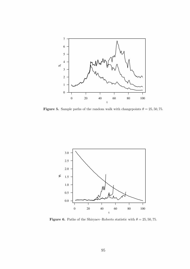
0 20 40 60 80 100
0
1
2
3
4
5
6
7
t
St
Figure 5. Sample paths of the random walk with changepoints 𝜃 = 25, 50, 75.
0 20 40 60 80 100
0.0
0.5
1.0
1.5
2.0
2.5
3.0
t
ψt
Figure 6. Paths of the Shiryaev–Roberts statistic with 𝜃 = 25, 50, 75.
95
References
[1] V. I. Arkin and I. V. Evstigneev. Stochastic Models of Control and
Economic Dynamics. Academic Press, London, 1987.
[2] M. Beibel and H. R. Lerche. A new look at optimal stopping problems
related to mathematical finance. Statistica Sinica, 7:93–108, 1997.
[3] F. Black and M. Scholes. The pricing of options and corporate liabilities.
The Journal of Political Economy, 81(3):637–654, 1973.
[4] Z. Bodie, R. C. Merton, and W. F. Samuelson. Labor supply flexibility
and portfolio choice in a life cycle model. Journal of Economic Dynamics
and Control, 16(3):427–449, 1992.
[5] L. Breiman. Optimal gambling systems for favorable games. In Proceed-
ings of the Fourth Berkeley Symposium on Mathematical Statistics and
Probability, volume I, pages 65–78. University of California Press, 1961.
[6] C. Castaing and M. Valadier. Convex Analysis and Measurable Multi-
functions. Springer, Berlin, 1977.
[7] A. S. Cherny. Pricing with coherent risk. Theory of Probability and Its
Applications, 52(3):389–415, 2008.
[8] S. A. Clark. The valuation problem in arbitrage price theory. Journal
of Mathematical Economics, 22(5):463–478, 1993.
[9] J. H. Cochrane and J. Saa-Requejo. Beyond arbitrage: good-deal as-
set price bounds in incomplete markets. Journal of Political Economy,
108(1):79–119, 2000.
[10] M. H. A. Davis and A. R. Norman. Portfolio selection with transaction
costs. Mathematics of Operations Research, 15(4):676–713, 1990.
96
[11] M. A. H. Dempster, I. V. Evstigneev, and M. I. Taksar. Asset pricing
and hedging in financial markets with transaction costs: an approach
based on the von Neumann – Gale model. Annals of Finance, 2(4):327–
355, 2006.
[12] E. B. Dynkin. Some probability models for a developing economy. Soviet
Mathematics Doklady, 12:1422–1425, 1971.
[13] E. B. Dynkin. Stochastic concave dynamic programming. Mathematics
of the USSR – Sbornik, 16(4):501, 1972.
[14] E. Ekstrom and C. Lindberg. Optimal closing of a momentum trade.
Journal of Applied Probability, 50(2):374–387, 2013.
[15] C. Esposito. The dangers of financial derivatives. Available at
http://www.highbeam.com/doc/1G1-295446185.html, June 2012.
[16] I. Evstigneev and M. Taksar. Stochastic equilibria on graphs I. Journal
of Mathematical Economics, 23(5):401–433, 1994.
[17] I. Evstigneev and M. Taksar. Stochastic equilibria on graphs II. Journal
of Mathematical Economics, 24(4):383–406, 1995.
[18] I. Evstigneev and M. Taksar. Equilibrium states of random economies
with locally interacting agents and solutions to stochastic variational
inequalities in ⟨𝐿1, 𝐿∞⟩. Annals of Operations Research, 114(1-4):145–
165, 2002.
[19] I. Evstigneev and M. Taksar. Dynamic interaction models of economic
equilibrium. Journal of Economic Dynamics and Control, 33(1):166–
182, 2009.
[20] I. V. Evstigneev. Controlled random fields on a directed graph. Theory
of Probability and Its Applications, 33(3):433–445, 1988.
[21] I. V. Evstigneev and K. R. Schenk-Hoppe. Handbook on Optimal
Growth, volume 1, chapter The von Neumann–Gale growth model and
its stochastic generalization, pages 337–383. Springer, Berlin, 2006.
97

[22] I. V. Evstigneev, K. Schurger, and M. I. Taksar. On the fundamen-
tal theorem of asset pricing: random constraints and bang-bang no-
arbitrage criteria. Mathematical Finance, 14(2):201–221, 2005.
[23] I. V. Evstigneev and M. V. Zhitlukhin. Controlled random fields,
von Neumann – Gale dynamics and multimarket hedging with risk.
Stochastics, 85(4):652–666, 2013.
[24] H. Follmer and A. Schied. Stochastic Finance: An Introduction in Dis-
crete Time. Walter de Gruyter, Berlin, 2002.
[25] D. Gale. The closed linear model of production. In Linear Inequalities
and Related Systems, volume 38 of Annals of Mathematical Studies,
pages 285–303. Princeton University Press, Princeton, 1956.
[26] D. Gale. A geometric duality theorem with economic applications. The
Review of Economic Studies, 34(1):19–24, 1967.
[27] D. Gale. On optimal development in a multi-sector economy. The Review
of Economic Studies, 34(1):1–18, 1967.
[28] P. V. Gapeev and G. Peskir. The Wiener disorder problem with finite
horizon. Stochastic Processes and Their Applications, 116(12):1770–
1791, 2006.
[29] D. C. Heath and R. A. Jarrow. Arbitrage, continuous trading, and
margin requirements. The Journal of Finance, 42(5):1129–1142, 1987.
[30] W. Hildenbrand. Core and Equilibria of a Large Economy. Princeton
university press, Princeton, 1974.
[31] J. C. Hull. Options, Futures, and Other Derivatives. Prentice Hall,
2011.
[32] E. Jouini and H. Kallal. Arbitrage in securities markets with short-sales
constraints. Mathematical Finance, 5(3):197–232, 1995.
[33] Yu. Kabanov and M. Safarian. Markets with Transaction Costs. Math-
ematical Theory. Springer, Berlin, 2009.
98

[34] D. Kahneman, J. L. Knetsch, and R. H. Thaler. Experimental tests
of the endowment effect and the Coase theorem. Journal of Political
Economy, 98:1325–1348, 1990.
[35] O. Kallenberg. Foundations of Modern Probability. Springer, 2002.
[36] I. Karatzas, J. P. Lehoczky, S. P. Sethi, and S. E. Shreve. Explicit so-
lution of a general consumption/investment problem. In Optimal Con-
sumption and Investment with Bankruptcy, pages 21–56. Springer, 1997.
[37] J. Kelly, Jr. A new interpretation of the information rate. Bell System
Technical Journal, 35:917–926, 1956.
[38] J. Komlos. A generalization of a problem of Steinhaus. Acta Mathemat-
ica Hungarica, 18(1):217–229, 1967.
[39] R. S. Liptser and A. N. Shiryaev. Statistics of Random Processes.
Springer, 2nd edition, 2000.
[40] L. C. MacLean, E. O. Thorp, and W. T. Ziemba, editors. The Kelly
Capital Growth Criterion: Theory and Practice. World Scientific, 2010.
[41] S. Mai. The global derivatives market. Deutsche Borse white paper,
April 2008.
[42] R. C. Merton. Lifetime portfolio selection under uncertainty: the
continuous-time case. The Review of Economics and Statistics,
51(3):247–257, 1969.
[43] I. Molchanov. Theory of Random Sets. Springer, 2005.
[44] A. J. Morton and S. R. Pliska. Optimal portfolio management with
fixed transaction costs. Mathematical Finance, 5(4):337–356, 1995.
[45] E. S. Page. Continuous inspection schemes. Biometrika, 41:100–114,
1954.
[46] E. S. Page. Control charts with warning lines. Biometrika, 42:243–257,
1955.
99
[47] G. Peskir and A. Shiryaev. Optimal Stopping and Free-Boundary Prob-
lems. Birkhauser Basel, 2006.
[48] R. Radner. Optimal stationary consumption with stochastic production
and resources. Journal of Economic Theory, 6(1):68–90, 1973.
[49] S. W. Roberts. Control charts based on geometric moving average.
Technometrics, 1:239–250, 1959.
[50] R. T. Rockafellar. Convex Analysis. Princeton University Press, Prince-
ton, 1972.
[51] L. C. G. Rogers. Arbitrage with fractional Brownian motion. Mathe-
matical Finance, 7(1):95–105, 1997.
[52] D. B. Rokhlin. The Kreps–Yan theorem for 𝐿∞. International Journal
of Mathematics and Mathematical Sciences, 17:2749–2756, 2005.
[53] A. Roux. The fundamental theorem of asset pricing in the presence of
bid-ask and interest rate spreads. Journal of Mathematical Economics,
47(2):159–163, 2011.
[54] W. Schachermayer. Private communication, 2012.
[55] W. Shewart. The application of statistics as an aid in maintaining
quality of a manufactured product. Journal of the American Statistical
Association, 20(152):546–548, 1925.
[56] A. Shiryaev and A. A. Novikov. On a stochastic version of the trading
rule ”Buy and Hold”. Statistics & Decisions, 26(4):289–302, 2009.
[57] A. N. Shiryaev. The detection of spontaneous effects. Soviet Mathemat-
ics Doklady, 2:740–743, 1961.
[58] A. N. Shiryaev. The problem of the most rapid detection of a disturbance
in a stationary process. Soviet Mathematics Doklady, 2:795–799, 1961.
[59] A. N. Shiryaev. On optimal methods in quickest detection problems.
Theory of Probability and Its Applications, 8(1):22–46, 1963.
100

[60] A. N. Shiryaev. On arbitrage and replication for fractal models. Tech-
nical report, MaPhySto, 1998.
[61] A. N. Shiryaev. Essentials of Stochastic Finance: Facts, Models, Theory.
World Scientific, Singapore, 1999.
[62] A. N. Shiryaev. Quickest detection problems in the technical analysis of
the financial data. In Mathematical Finance – Bachelier Congress 2000,
pages 487–521. Springer, 2002.
[63] A. N. Shiryaev. Probability. MCCME, Moscow, 3rd edition, 2004. In
Russian.
[64] A. N. Shiryaev. Optimal stopping rules. Springer, 2007.
[65] A. N. Shiryaev. Quickest detection problems: fifty years later. Sequential
Analysis, 29(4):445–385, 2010.
[66] A. N. Shiryaev, M. V. Zhitlukhin, andW. T. Ziemba. When to sell Apple
and the NASDAQ? Trading bubbles with a stochastic disorder model.
Accepted for publication in The Journal of Portfolio Management, 2013.
[67] T. Sottinen. Fractional Brownian motion, random walks and binary
market models. Finance and Stochastics, 5(3):343–355, 2001.
[68] J. von Neumann. Uber ein okonomisches Gleichungssystem und eine
Verallgemeinerung des Brouwerschen Fixpunktsatzes. Ergebnisse Eines
Mathematischen Kolloquiums, 8:73–83, 1937.
[69] M. V. Zhitlukhin and A. N. Shiryaev. Bayesian disorder detection prob-
lems on filtered probability spaces. Theory of Probability and Its Appli-
cations, 57(3):497–511, 2013.
101


![A hybrid smoothed dissipative particle dynamics (SDPD ...the deterministic spatial dynamics but not the stochastic dynamics. The spatial stochastic simulation 80 algorithm (sSSA) [29]](https://img.pdfslide.net/doc/110x75/5f41a2ab66492703c57addfe/a-hybrid-smoothed-dissipative-particle-dynamics-sdpd-the-deterministic-spatial.jpg)