Embed Size (px)
Citation preview
Stochastic growth
Martin Ellison
1 Motivation
In this lecture we apply the techniques of dynamic programming to real
macroeconomic problems. We use the technique of value function iterations
to derive the solution of the stochastic growth model, in which a representa-
tive agent makes optimal choices between current consumption and investing
in a productive asset, capital. To fully understand the intuition behind our
results and methods, we begin by analysing a simple non-stochastic growth
model and presenting Gauss codes to solve the model numerically by com-
puter. The stochastic version of the growth model is presented in the latter
half of the lecture. In this case, a simple stochastic structure is sufficient to
demonstrate the theoretical concepts and numerical simulation.
2 Key reading
The majority of this lecture is derived from chapter 5 of “Dynamic Eco-
nomics: Quantitative Methods and Applications” by Jérôme Adda and Rus-
sell Cooper, Massachusetts Institute of Technology, 2003.
1
3 Other reading
The stochastic growth model and its solution are covered in almost all ad-
vanced textbooks in macroeconomics. The relevant chapter of “Recursive
Macroeconomic Theory”, 2nd ed by Lars Ljungqvist and Tom Sargent, MIT
Press, 2000, is number 11.The analytical result with full depreciation is well
known from “Dynamic Macroeconomic Theory” by Tom Sargent, Harvard
University Press, 1987.
4 Non-stochastic growth model
In the non-stochastic growth model, the problem of the representative agent
is to allocate resources between consumption �� and investment in capital ��,
as in the continuous time Ramsey model. Capital is completely malleable,
being able to be transformed into consumption at a rate of one-to-one. Since
the model is deterministic, there is no uncertainty. Consumption gives in-
stantaneous utility through the function �(��), which is strictly increasing
and strictly concave. Capital is productive according to the production func-
tion �� = �(��), which is similarly strictly increasing and strictly concave.
Capital stored depreciates at the rate � when used in production. With the
representative agent discounting future utility at the rate �, the problem is
as follows:
max{��}
∞P�=1
��−1�(��)
�
�� = �(��)
�� = �� + ��
��+1 = ��(1− �) + ��
2

where �� is gross investment. Taking our now familiar dynamic program-
ming approach, we can write the value function as
� (�) = max�0[�(�(�) + (1− �)� − �0) + �� (�0)]
The first order condition is
�0(�) = �� 0(�0)
As in the previous lecture, we do not know the form is the value function
� (�), but we do know its first derivative � 0(�). Differentiating from the
definition of the value function
� 0(�) = �0(�) [� 0(�) + (1− �)]Rolling forward one period
� 0(�0) = �0(�0) [� 0(�0) + (1− �)]Substitute in the first order condition
�0(�) = ��0(�0) [� 0(�0) + (1− �)]This is the Euler equation for optimal consumption smoothing in the non-
stochastic growth model, analogous to the Euler equation in the cake-eating
example of the previous lecture. It is economically intuitive. the left hand
side shows the utility benefit of increasing consumption by one unit in the
current period. The right hand side shows the benefit of postponing con-
sumption to the next period. One unit of consumption postponed increases
the productive capital next period by one unit, and so generates extra output
� 0(�0). However, the extra capital depreciates during production so that the
net additional consumption available is � 0(�0)+(1−�). This is then weighted
3
by the marginal utility of consumption to arrive at the utility benefit of the
extra consumption. It is discounted by � because the extra consumption
only occurs in the next period.
To proceed from the value function and first order conditions, we have
three options. Firstly, it may be possible to solve the problem analytically by
guessing the form of the value function or policy function. Secondly, we could
linearise or log-linearise the first order conditions to obtain an approximate
solution. Thirdly, we can apply value function iterations to derive a numer-
ical solution. In this lecture, we will investigate the first and third options.
The second option, approximation, is beyond the scope of the this course,
although its is not conceptually difficult. Interested readers are referred to
“Recursive Methods for Computing Equilibria of Business Cycle Models” by
Gary Hansen and Ed Prescott in “Frontiers of Business Cycle Research”,
edited by Tom Cooley, PUP, 1995. The book “Computational Methods for
the Study of Dynamic Economies”, edited by Ramon Marimon and Andrew
Scott, CUP, 1999, is also a good reference.
5 An analytically tractable non-stochastic growth
model example
In general, it is not possible to solve analytically for the value function and
policy function. However, it is possible under very strict assumptions. We
begin by defining functional forms for the utility function and production
function.
�(�) = ln �
�(�) = ��
These functional forms are fairly standard, although the production func-
4
tion does preclude the use of labour as a factor of production. Our final as-
sumption is even less realistic. We assume � = 1 so that capital depreciation
occurs at the rate of 100%. In other words, any capital saved to the next
periods depreciates completely after production. The intertemporal budget
constraint is therefore �0 = � rather that �0 = �(1 − �) + �. We begin oursolution by making a guess at the form of the value function.
� (�) = +� ln �
This is an informed, rather than random, guess because we know that
the state variable is � and both the utility and production functions are
logarithmic. We proceed to confirm this is correct by showing that, if this is
the correct form of the value function, optimising behaviour implies a value
function of the same form. If the value function is correct, the first order
condition �0(�) = �� 0(�0) implies
1
�=��
�
The budget constraint and 100% depreciation define
�� = �+ �0
Solving these equations, we can obtain expressions for the policy functions
of consumption and future capital.
� =
µ1
1 + ��
¶��
�0 =
µ��
1 + ��
¶��
We now return to the value function and show that these policy functions
are consistent with a value function of the form originally posited.
5
� (�) = +� ln � = ln
·µ1
1 + ��
¶��¸+ �
· +� ln
·µ��
1 + ��
¶��¸¸
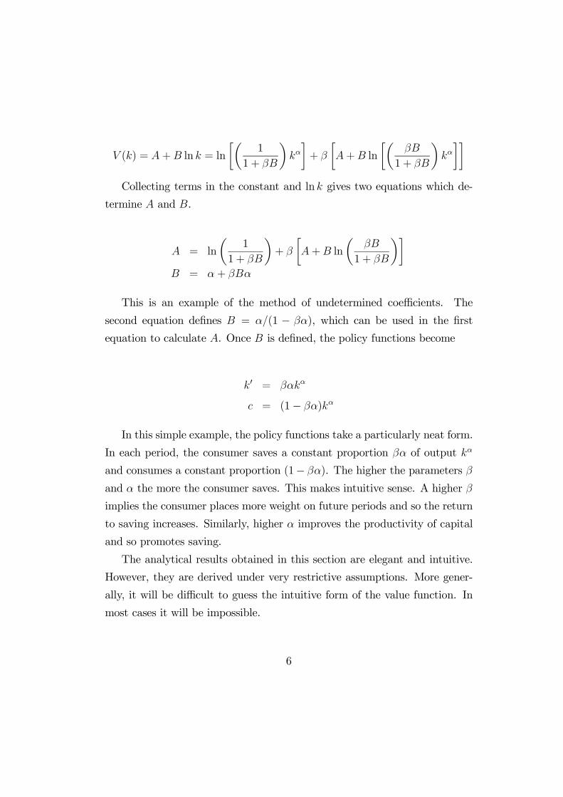
Collecting terms in the constant and ln � gives two equations which de-
termine and �.
= ln
µ1
1 + ��
¶+ �
· +� ln
µ��
1 + ��
¶¸� = � + ���
This is an example of the method of undetermined coefficients. The
second equation defines � = ��(1 − ��), which can be used in the firstequation to calculate . Once � is defined, the policy functions become
�0 = ����
� = (1− ��)��
In this simple example, the policy functions take a particularly neat form.
In each period, the consumer saves a constant proportion �� of output ��
and consumes a constant proportion (1− ��). The higher the parameters �and � the more the consumer saves. This makes intuitive sense. A higher �
implies the consumer places more weight on future periods and so the return
to saving increases. Similarly, higher � improves the productivity of capital
and so promotes saving.
The analytical results obtained in this section are elegant and intuitive.
However, they are derived under very restrictive assumptions. More gener-
ally, it will be difficult to guess the intuitive form of the value function. In
most cases it will be impossible.
6

6 Numerical non-stochastic growthmodel ex-
ample
Our numerical example maintains the same function form for the production
function but uses the more general CRRA utility function with coefficient �
equal to the coefficient of relative risk aversion.
�(�) =�1−�
1− ��(�) = ��
In the limit of �→ 1, the utility function becomes logarithmic as before.
In contrast to the analytical example, we allow depreciation to be less than
100% so we have a full set of dynamic equations showing how state variables
evolve.
� = �+ �
�0 = �(1− �) + �The numerical code below solves for repeated iterations of the value func-
tion.
� (� )(�) = max�0[�(�(�) + (1− �)� − �0) + �� (�0)]
We do not check Blackwell’s sufficiency conditions for a contraction map-
ping since monotonicity and discounting hold by the same arguments ex-
pressed in the previous lecture. The computer program is written in Matlab
and the code complimentary is available from the homepage of the Adda and
Cooper book at
http://www.eco.utexas.edu/~cooper/dynprog/dynprog1.html
7
There are four main parts to the code: parameter value initialisation,
state space definitions, value function iterations and output.
Start new program by clearing the work space. Parameters are initialised
with beta the discount factor, sigma the coefficient of relative risk aversion,
alpha the exponent on capital in the production function and delta the de-
preciation rate.
CLEAR;
beta=0.9;
sigma=1;
alpha=0.75;
delta=0.3;
We now construct a grid of possible capital stocks. The grid is centred
on the steady-state capital stock �∗, which is obtained from the steady-state
value of the Euler equation of the stochastic growth model. We have
�0(�∗) = ��0(�∗) [� 0(�∗) + (1− �)]With � 0(�∗) = ��∗�−1, this reduces to
1 = �£��∗�−1 + (1− �)¤
Solving for �∗.
�∗ =µ1
��− 1− �
�
¶ 1�−1
The grid is centred around this point, with maximum (���) and minimum
(���) values 110% and 90% of the steady-state value. There are � discrete
points in the grid.
8
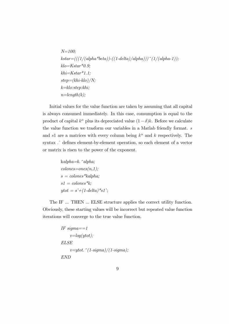
N=100;
kstar=(((1/(alpha*beta))-((1-delta)/alpha)))^(1/(alpha-1));
klo=Kstar*0.9;
khi=Kstar*1.1;
step=(khi-klo)/N;
k=klo:step:khi;
n=length(k);
Initial values for the value function are taken by assuming that all capital
is always consumed immediately. In this case, consumption is equal to the
product of capital �� plus its depreciated value (1− �)�. Before we calculatethe value function we trasform our variables in a Matlab friendly format. �
and �1 are a matrices with every column being �� and � respectively. The
syntax ˆ defines element-by-element operation, so each element of a vector
or matrix is risen to the power of the exponent.
kalpha=k.^alpha;
colones=ones(n,1);
s = colones*kalpha;
s1 = colones*k;
ytot = s’+(1-delta)*s1’ ;
The IF ... THEN ... ELSE structure applies the correct utility function.
Obviously, these starting values will be incorrect but repeated value function
iterations will converge to the true value function.
IF sigma==1
v=log(ytot);
ELSE
v=ytot.^(1-sigma)/(1-sigma);
END
9
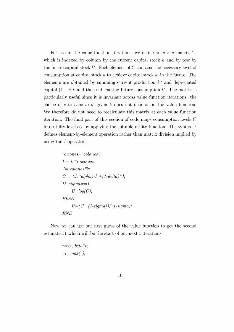
For use in the value function iterations, we define an � × � matrix �,which is indexed by column by the current capital stock � and by row by
the future capital stock �0. Each element of � contains the necessary level of
consumption at capital stock � to achieve capital stock �0 in the future. The
elements are obtained by summing current production �� and depreciated
capital (1− �)� and then subtracting future consumption �0. The matrix isparticularly useful since it is invariant across value function iterations: the
choice of � to achieve �0 given � does not depend on the value function.
We therefore do not need to recalculate this matrix at each value function
iteration. The final part of this section of code maps consumption levels �
into utility levels � by applying the suitable utility function. The syntax �
defines element-by-element operation rather than matrix division implied by
using the � operator.
rowones= colones’;
I = k’*rowones;
J= colones*k;
C = (J.^alpha)-I +(1-delta)*J;
IF sigma==1
U=log(C);
ELSE
U=(C.^(1-sigma))/(1-sigma);
END
Now we can use our first guess of the value function to get the second
estimate �1 which will be the start of our next iterations.
r=U+beta*v;
v1=max(r);
10

For each iteration, the �� matrix �1 collects the consequences of differ-ent actions at different initial capital levels. Each column of � corresponds
to a given initial capital stock level �. The rows of �1 then show the value
of leaving different future capital stocks �0. The value of each choice is ob-
tained by summing the value of the implied consumption level (from the
utility matrix �) and the value of carrying forward capital �0 to the next
period (from the value function �1 derived in the previous iteration). Once
the consequences of different actions have been collected in �1, the value
function iteration proceeds by selecting the maximum value form each of its
columns. As these values are implicitly stored as a row vector we line them
up vertically into a matrix �. This matrix becomes the next iteration of the
value function.
t=100
FOR j=1:t
w=ones(n,1)*v1;
w1=U+beta*w’;
v1=max(w1);
END
Value function iterations are now complete. The final value function is
stored in � �� and the indices of the future �0 choices are stored in ���. These
latter indices are converted into �0 values in ���.
[val,ind]=max(w1);
optk = K(ind);
To illustrate the results, it is useful to plot how �0 varies as a function of
�. This is the policy function in Figure 5.1 of Adda and Cooper.
figure(1)
11
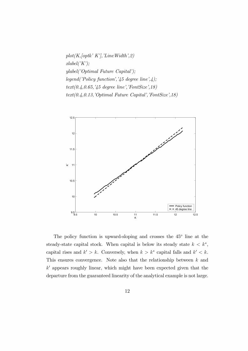
plot(K,[optk’ K’],’LineWidth’,2)
xlabel(’K’);
ylabel(’Optimal Future Capital’);
legend(’Policy function’,’45 degree line’,4);
text(0.4,0.65,’45 degree line’,’FontSize’,18)
text(0.4,0.13,’Optimal Future Capital’,’FontSize’,18)
9.5 10 10.5 11 11.5 12 12.59.5
10
10.5
11
11.5
12
12.5
K
K`
Policy function45 degree line
The policy function is upward-sloping and crosses the 45� line at the
steady-state capital stock. When capital is below its steady state � �∗,
capital rises and �0 ! �. Conversely, when � ! �∗ capital falls and �0 �.
This ensures convergence. Note also that the relationship between � and
�0 appears roughly linear, which might have been expected given that the
departure from the guaranteed linearity of the analytical example is not large.
12

A second useful figure is Figure 5.2 from Adda and Cooper, showing net
investment �0−� as a function of �. The figure confirms that net investmentis positive when � �∗ and negative when � ! � ∗.
figure (2)
plot(K,(optk-k)’,’LineWidth’,2)
xlabel(’K’);
ylabel(’K‘ - K’);
9.5 10 10.5 11 11.5 12 12.5-0.2
-0.15
-0.1
-0.05
0
0.05
0.1
0.15
K
K` -
K
To gain an insight into the dynamics of the adjustment process, it is
useful to calculate the path of convergence of capital if initial capital is not
equal to its steady-state value. The exercise is similar to the tracing out of
impulse response functions in a structural vector autoregression analysis. �
13
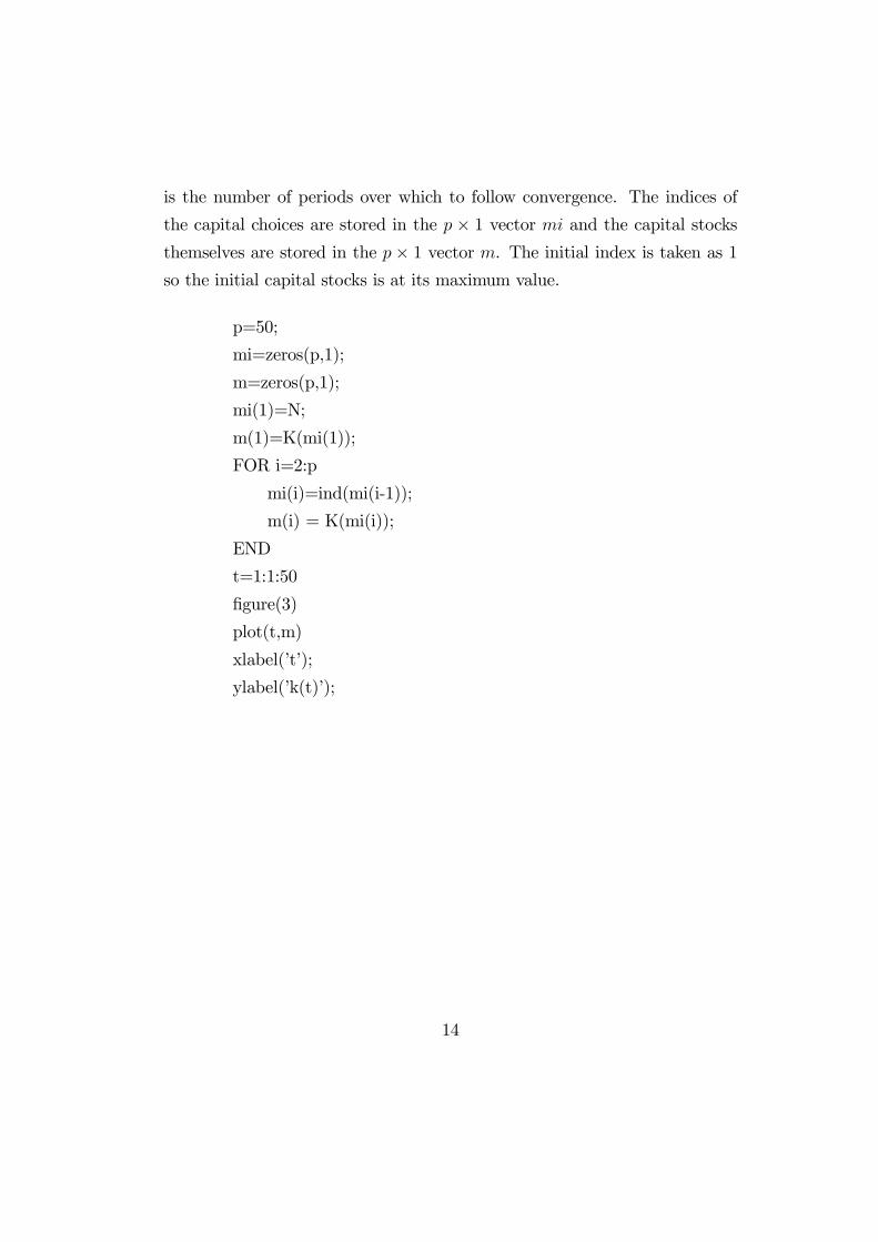
is the number of periods over which to follow convergence. The indices of
the capital choices are stored in the � × 1 vector "� and the capital stocksthemselves are stored in the �× 1 vector ". The initial index is taken as 1so the initial capital stocks is at its maximum value.
p=50;
mi=zeros(p,1);
m=zeros(p,1);
mi(1)=N;
m(1)=K(mi(1));
FOR i=2:p
mi(i)=ind(mi(i-1));
m(i) = K(mi(i));
END
t=1:1:50
figure(3)
plot(t,m)
xlabel(’t’);
ylabel(’k(t)’);
14
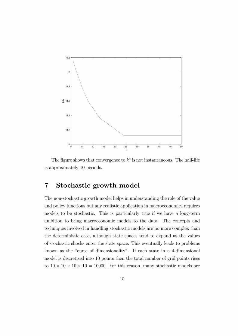
0 5 10 15 20 25 30 35 40 45 5011
11.2
11.4
11.6
11.8
12
12.2
t
k(t)
The figure shows that convergence to �∗ is not instantaneous. The half-life
is approximately 10 periods.
7 Stochastic growth model
The non-stochastic growth model helps in understanding the role of the value
and policy functions but any realistic application in macroeconomics requires
models to be stochastic. This is particularly true if we have a long-term
ambition to bring macroeconomic models to the data. The concepts and
techniques involved in handling stochastic models are no more complex than
the deterministic case, although state spaces tend to expand as the values
of stochastic shocks enter the state space. This eventually leads to problems
known as the “curse of dimensionality”. If each state in a 4-dimensional
model is discretised into 10 points then the total number of grid points rises
to 10 × 10 × 10 × 10 = 10000. For this reason, many stochastic models are
15
kept to a small scale.
Our stochastic version of the growth model incorporates shocks to pro-
duction technology that enter multiplicatively in the production function.
Commonly known as the Solow residual, � accounts for unexplained changes
in productivity. It changes the problem of the representative agent to be
max{��}
∞P�=1
��−1�(��)
�
�� = ��(��)
�� = �� + ��
��+1 = ��(1− �) + ��
Without loss of generality, we restrict our attention to stochastic processes
for � that are Markovian, i.e. � is a sufficient statistic to form the expec-
tation of �+1. In dynamic programming form, the value function is defined
by the Bellman equation.
� ( # �) = max�0
£�( �(�) + (1− �)� − �0) + �$�0|�� ( 0# �0)
¤Compared with the non-stochastic growth model, there are two changes.
Firstly, the value function has two arguments: the current level of technology
and the current capital stock �. Secondly, the continuation part of the
value function is only defined in terms of an expectation. It is the expected
continuation value, where the expectation is evaluated across the distribution
of future technology 0 given current technology . The expectations remains
in the first order condition.
�0(�) = �$�0|� [�0(�0)( 0�(�0) + (1− �))]
16
It is possible to solve this problem analytically as before for the limiting
case of 100% depreciation and logarithmic utility. Such an exercise is left for
the reader. Instead, we jump straight to a numerical solution of a stochastic
growth model through value function iterations.
8 Numerical stochastic growth model exam-
ple
To maintain comparability with the non-stochastic growth model example,
we use the same function forms for the utility and production functions.
�(�) =�1−�
1− ��(�) = ��
We introduce a stochastic element to in the simplest possible manner.
We assume technology can either be high ̄ or low A¯with equal probability,
i.e.
0 = ̄ with probability 0.5
0 = A¯with probability 0.5
As a more general case, one could imagine having a range of discrete
values for 0 with different probabilities. In this way, the distribution of 0
could be matched, say, to a normal distribution. The way we have defined
the stochastic element means that the distribution of 0 is independent of .
Economically, this is equivalent to saying that technology shocks only have
a temporary and not permanent or persistent effects. It is simple (although
not trivial) to extend the computer code to handle persistent shocks.
17

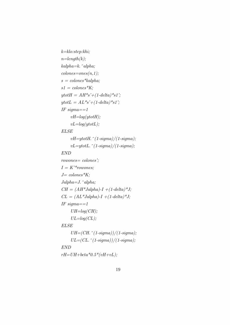
The main difference to the computer code is that policy functions and
value functions become � × 2 matrices, with the columns corresponding topolicy and value functions conditional on high or low current productivity.
We can write out the expectation in the value function as follows:
� ( # �) = max�0
·�( �(�) + (1− �)� − �0) + �
2
£� ( ̄# �0) + � (A
¯# �0)
¤¸This Bellman equation forms the basis of the value function iterations.
In practical terms, for each iteration we use the matrices �% and �& for
the consumption levels necessary to achieve future capital �0 when current
capital is � and current technology is high and low respectively. �% and �&
are the associated utility levels.
CLEAR ALL
sigma=1;
beta=0.9;
alpha=.75;
delta=0.3;
AH=1;
AL=0.99;
N=100;
kstarH=(((1/(AH*alpha*beta))-((1-delta)/(AH*alpha))))^(1/(alpha-
1));
kstarL=(((1/(AL*alpha*beta))-((1-delta)/(AL*alpha))))^(1/(alpha-
1));
kstar=0.5*(KstarH+KstarL);
klo=kstar*0.9;
khi=kstar*1.1;
step=(khi-klo)/N;
18
k=klo:step:khi;
n=length(k);
kalpha=k.^alpha;
colones=ones(n,1);
s = colones*kalpha;
s1 = colones*K;
ytotH = AH*s’+(1-delta)*s1’;
ytotL = AL*s’+(1-delta)*s1’;
IF sigma==1
vH=log(ytotH);
vL=log(ytotL);
ELSE
vH=ytotH.^(1-sigma)/(1-sigma);
vL=ytotL.^(1-sigma)/(1-sigma);
END
rowones= colones’;
I = K’*rowones;
J= colones*K;
Jalpha=J.^alpha;
CH = (AH*Jalpha)-I +(1-delta)*J;
CL = (AL*Jalpha)-I +(1-delta)*J;
IF sigma==1
UH=log(CH);
UL=log(CL);
ELSE
UH=(CH.^(1-sigma))/(1-sigma);
UL=(CL.^(1-sigma))/(1-sigma);
END
rH=UH+beta*0.5*(vH+vL);
19

rL=UL+beta*0.5*(vH+vL);
vH1=max(rH);
vL1=max(rL);
t=100
FOR j=1:t
w=ones(n,1)*(vH1+vL1);
wH1=UH+beta*0.5*w’;
wL1=UL+beta*0.5*w’;
vH1=max(wH1);
vL1=max(wL1);
END
[valH,indH]=max(wH1);
[valL,indL]=max(wL1);
optkh = K(indH);
optkl = K(indL);
FIGURE(1)
plot(K,[K’ optkh’ optkl’],’LineWidth’,2)
xlabel(’K’);
ylabel(’K‘’);
legend(’45 degree line’,’Policy function- High Tech’,’Policy function-
Low Tech’,4);
FIGURE(2)
plot(K,[(optkh-K)’ (optkl-K)’],’LineWidth’,2)
xlabel(’K’);
ylabel(’K‘- K’);
20

9.5 10 10.5 11 11.5 129.5
10
10.5
11
11.5
12
K
K` Policy function- High Tech
45 degree line
Policy function- Low Tech
9.5 10 10.5 11 11.5 12-0.2
-0.15
-0.1
-0.05
0
0.05
0.1
0.15
K
K`- K
High Technology
Low Technology
The policy function figures now have two lines, each corresponding to
policy conditional on current productivity. In the figures, the higher line is
for high technology and the lower line is for low technology. The dynamics
21

of the system will change according to the value of . The system is globally
stable since for very low capital stocks the capital stock is always increasing
and for very high capital stocks the capital stock is always decreasing. For
intermediate levels of the capital stock, the system converges in distribution
if not to a fixed point.
To appreciate the dynamics of the system, we present a simple simulation
of the evolution of the capital stock over � periods. Initial capital stock is
taken to be at the average steady-state value. The function ' �((1# 1)
draws a single random number from the uniform distribution [0# 1]. By com-
paring its value with 0.5, we are able to draw shocks from the stochastic
distribution of . A typical stochastic simulation is shown below. We also
print out the standard deviations of output, consumption and investment.
p=500;
kt=Kstar*ones(p,1);
kti=(N/2)*ones(p,1);
FOR i=2:p
IF RAND(1,1)!0.5
yt(i)=AH*(kt(i-1))^alpha;
kti(i)=indH(kti(i-1));
kt(i)=K(kti(i));
ELSE
yt(i)=AL*(kt(i-1))^alpha;
kti(i)=indL(kti(i-1));
kt(i)=K(kti(i));
END
ct(i)=yt(i)+(1-delta)*kt(i-1)-kt(i);
it(i)=yt(i)-ct(i);
END
22

t=1:1:500;
figure (3)
plot(t,kt)
xlabel(’t’);
ylabel(’k(t)’);
syt=std(yt(10:p));
sct=std(ct(10:p));
si=std(it(10:p));
0 50 100 150 200 250 300 350 400 450 50010.7
10.75
10.8
10.85
10.9
10.95
11
11.05
t
k(t)
Variable SD
� 0.041
� 0.015
� 0.029
23

Even with such a simple example, the simulation results are highly infor-
mative. Consumption is by far the least volatile variable, reflecting strong
incentives for consumption smoothing in the model. Analysis of more com-
plex models in this way has been a bedrock of Real Business Cycle research
since the seminal contribution of Kydland and Prescott in Econometrica in
1982.
24