Stochastic interest rates and the q theory of investment∗

Neng Wang† Jinqiang Yang‡

October 12, 2011

Abstract

The interest rate is a key determinant of firm investment. We integrate a widely-used term structure model of interest rates, CIR (Cox, Ingersoll, and Ross (1985)),with the q theory of investment (Hayashi (1982) and Abel and Eberly (1994)). Weshow that stochastic interest rates have significant effects on investment and firm valuebecause capital is medium/long lived. Capital adjustment costs have a first-order effecton investment and firm value. We use duration to measure the interest rate sensitivityof firm value, and decompose a firm into assets in place and growth opportunities,and value each component. By extending the model to allow for endogenous capitalliquidation, we find that the liquidation option provides a valuable protection againstthe increase of interest rates. We further generalize the model to incorporate asym-metric adjustment costs, a price wedge between purchasing and selling capital, fixedinvestment costs, and irreversibility. We find that inaction is often optimal for an em-pirically relevant range of interest rates for firms facing fixed costs or price wedges.Finally, marginal q is equal to average q in our stochastic interest rate settings, includ-ing one with serially correlated productivity shocks.

Keywords: term structure of interest rates, adjustment costs, average q, marginal q,duration, assets in place, growth opportunities, fixed costs, irreversibility, price wedges

JEL Classification: E2, G31, G12

∗Comments are welcome!†Columbia University and NBER. Email: neng.wang@columbia.edu. Tel.: 212-854-3869.‡Columbia University and Shanghai University of Finance and Economics (SUFE).

1 Introduction

If a firm can frictionlessly adjust its capital stock, its investment in each period is essentially

a static choice of “target” capital stock, which optimally equates the marginal product of

capital with the user cost of capital (Jorgenson (1963)). However, changing capital stock

often incurs various adjustment costs. Installing new equipment or upgrading capital may

require time and resources, and lead to disruptions in production lines. Workers need to go

through a costly learning process to operate newly installed capital. The complete/partial

irreversibility of business projects is another type of adjustment cost. Lacking secondary

markets for capital may generate a price wedge between purchasing and selling capital.

Additionally, informational asymmetries and agency conflicts distort investment, which may

be captured by adjustment costs as an approximation. These frictions, modeled by various

capital adjustment costs, prevent the firm from instantaneously adjusting its capital stock

to the target level, and make the firm’s investment decision intrinsically dynamic.

The intertemporal optimizing framework with capital adjustment costs is often referred

to as the q theory of investment.1 Almost all existing work in the q literature assumes that

interest rates are constant over time. However, interest rates are persistent, volatile, and

carry risk premia. Additionally, physical capital is medium- and/or long-term lived, making

the value of capital sensitive to movements of interest rates. Moreover, adjustment costs

make capital illiquid and hence capital carries an additional illiquidity premium. We are

thus motivated to augment the conventional q theory with stochastic interest rates. We

achieve this objective by integrating a widely-used term structure model of interest rates,

the CIR (Cox, Ingersoll, and Ross (1985)) model, with a stochastic version of the seminal

Hayashi (1982) model in the q theory literature.

Our baseline model includes minimal but essential elements. The firm faces convex

capital adjustment costs and operates a constant return to scale production technology

with independently and identically distributed (iid) productivity shocks. For simplicity, we

assume that the adjustment cost function is homogeneous in investment and capital as in

Lucas and Prescott (1971) and Hayashi (1982). The interest rate process is governed by the

CIR term structure model. Even with stochastic interest rates, our framework generates the

1Abel and Eberly (1994) develop a unified neoclassic q theory of investment. Lucas and Prescott (1971),Mussa (1977), Lucas (1981), Hayashi (1982), and Abel (1983) are important early contributors. See Caballero(1999) for a survey on investment.

1

result that the marginal q is equal to Tobin’s average q,2 thus extending the condition for

this equality result given by Hayashi (1982) in a deterministic setting to a stochastic interest

rate environment. Our parsimonious framework yields tractable solutions for investment and

firm value. We derive an ordinary differential equation (ODE) for Tobin’s q. As we expect,

investment and firm value are decreasing and convex in interest rates.

Existing q models generate rich investment behavior from interactions between persistent

productivity shocks and adjustment costs, but under constant interest rates. These models

work through the cash flow channel. Unlike them, we focus on the effects of stochastic interest

rates on firm value and investment, by intentionally choosing iid productivity shocks to rule

out the effects of time-varying investment opportunities. Time-series variation of investment

and q in our model thus is driven by interest rates. Empirically, both productivity shocks and

interest rates are likely to have significant effects. Our work thus complements the existing

literature by demonstrating the importance of the interest rate channel.

Calibrating our model to the US data, we find that interest rates and adjustment costs

interact with each other and have quantitatively significant effects on investment and firm

value. As in fixed-income analysis, we use duration to measure the interest rate sensitivity of

firm value. We decompose a firm into assets in place and growth opportunities (GO). While

the value of assets in place decreases with interest rates for the standard discount rate effect,

the value of GO may either decrease or increase with interest rates due to two opposing

effects. In addition to the standard discount rate effect, there is also a cash flow effect

for GO: increasing interest rates discourages investment, lowers adjustment costs, and thus

increases the firm’s expected cash flows and the value of GO, ceteris paribus. As adjustment

costs increase, capital becomes more illiquid and the relative weight of assets in place in

firm value increases. In the limit, with infinity adjustment costs and thus completely illiquid

capital, the firm is simply its assets in place with no GO.

For simplicity, we have chosen the widely-used convex adjustment costs for the baseline

model. However, investment frictions may not be well captured by symmetric convex adjust-

ment costs. For example, increasing capital stock is often less costly than decreasing capital

stock, thus suggesting an asymmetric adjustment cost. Additionally, the firm may pay fixed

costs when investing, may face a price wedge between purchase and sale prices of capital,

2Tobin’s average q is the ratio between the market value of capital to its replacement cost, which wasoriginally proposed by Brainard and Tobin (1968) and Tobin (1969) to measure a firm’s incentive to invest.

2

and investment may be completely or partially irreversible. Optimal investment may thus

be lumpy and inaction may sometimes be optimal. Abel and Eberly (1994) develop a unified

q theory of investment with a rich specification of adjustment costs.3 We further generalize

our baseline model with stochastic interest rates by incorporating a much richer specification

of adjustment costs as in Abel and Eberly (1994).

If a firm can liquidate its capital at a scrap value, it will optimally choose the liquidation

strategy which provides a valuable protection against the increase of interest rates. For a

firm facing either fixed costs or a price wedge between purchase and sale of capital, the firm’s

optimal investment policy is generally characterized by three regions: positive investment,

inaction, and divestment, with endogenously determined interest rate cutoff levels. Positive

investment is optimal when interest rates are sufficiently low. At high interest rates, the firm

optimally divests. For intermediary interest rates between these two cutoff levels, inaction

is optimal. We further extend our model to a regime-switching setting with persistent

productivity shocks. Despite stochastic interest rates and a wide array of adjustment costs,

our model has the property that the marginal q is equal to Tobin’s average q in all settings.

2 Model setup

We generalize the neoclassic q theory of investment to incorporate the effects of stochastic

interest rates on investment and firm value.

Physical production and investment technology. A firm uses its capital to produce

output.4 Let K and I denote respectively its capital stock and gross investment. Capital

accumulation is given by

dKt = (It − δKt) dt, t ≥ 0, (1)

where δ ≥ 0 is the rate of depreciation for capital stock.

The firm’s operating revenue over time period (t, t+dt) is proportional to its time-t capital

stock Kt, and is given by KtdXt, where dXt is the firm’s productivity shock over the same

3Stokey (2009) provides a modern textbook treatment of the economics of optimal inaction in acontinuous-time framework.

4The firm may use both capital and labor as factors of production. As a simple example, we may embeda static labor demand problem within our dynamic optimization. We will have an effective revenue functionwith optimal labor demand. The remaining dynamic optimality will be the same as the one in q theory. SeeAbel and Eberly (2011) for an example of such a treatment.

3

time period (t, t + dt). After incorporating the systematic risk for the firm’s productivity

shock, we may write the productivity shock dXt under the risk-neutral measure5 as follows,

dXt = πdt+ εdZt, t ≥ 0, (2)

where Z is a standard Brownian motion. The productivity shock dXt specified in (2) is

independently and identically distributed (iid). The constant parameters π and ε > 0 give

the corresponding (risk-adjusted) productivity mean and volatility per unit of time.

The firm’s operating profit dYt over the same period (t, t+ dt) is given by

dYt = KtdXt − C(It, Kt)dt, t ≥ 0, (3)

where C(I,K) is the total cost of the investment including both the purchase cost of the

investment good and the additional adjustment costs of changing capital stock. The firm

may sometimes find it optimal to divest and sell its capital, i.e. I < 0. Importantly, capital

adjustment costs make installed capital more valuable than new investment goods. The ratio

between the market value of capital and its replacement cost, often referred to as Tobin’s q,

provides a measure of rents accrued to installed capital. The capital adjustment cost plays

a critical role in the neoclassical q theory of investment.

For analytical simplicity, we assume that the firm’s total investment cost is homogeneous

of degree one in I and K, and write as follows,

C (I,K) = c(i)K, (4)

where i = I/K is the investment-capital ratio, and c(i) is an increasing and convex func-

tion.6 The convexity of c( · ) implies that the marginal cost of investing CI(I,K) = c′(i)

is increasing in i, and hence encourages the firm to smooth investment over time, ceteris

paribus. The production specification (1)-(4) features the widely used “AK” technology and

the homogeneous adjustment cost function in macroeconomics.

5The risk-neutral measure incorporates the impact of the interest rate risk on investment and firm value.6Lucas (1981), Hayashi (1982), and Abel and Blanchard (1983) specify the adjustment cost to be convex

and homogenous in I and K. While in this paper, we have specified the adjustment cost on the “cost” side,we can also effectively specify the effect of adjustment costs on the “revenue” side by choosing a concaveinstallation function in the “drift” of the capital accumulation equation (1) and obtain effectively similarresults. See Lucas and Prescott (1971), Baxter and Crucini (1993), and Jermann (1998) for examples whichspecify the adjustment cost via a concave installation function for capital from one period to the next.

4

Stochastic interest rates. While much work in the q theory context assumes constant

interest rates, empirically, there is much time-series variation in interest rates. Additionally,

the interest rate movement is persistent and has systematic risk. Moreover, the investment

payoffs are often long term in nature and hence cash flows from investment payoffs are sen-

sitive to the expected change and volatility of interest rates. In sum, interest rate dynamics

and risk premium have significant impact on investment and firm value.

Researchers often analyze effects of interest rates via comparative statics with respect

to interest rates (using the solution from a dynamic model with a constant interest rate).

While potentially offering insights, the comparative static analysis is unsatisfactory because

it ignores the dynamics and the risk premium of interest rates. By explicitly incorporating

a term structure of interest rates, we analyze the persistence and volatility effects of interest

rates on investment and firm value in a fully specified dynamic stochastic framework.

We choose the widely-used CIR model, which specifies the following dynamics for r:

drt = µ(rt)dt+ σ(rt)dBt, t ≥ 0, (5)

where B is a standard Brownian motion under the risk-neutral measure, and the risk-neutral

drift µ(r) and volatility σ(r) are respectively given by

µ(r) = κ(ξ − r), (6)

σ(r) = ν√r. (7)

Both the (risk-adjusted) conditional mean and the conditional variance of the interest rate

change are linear in r. The parameter κ measures mean reversion of interest rates. The

implied first-order autoregressive coefficient in the corresponding discrete-time model is e−κ.

The higher κ, the more mean-reverting. The parameter ξ is the long-run mean of interest

rates. The CIR model captures the mean-reversion and conditional heteroskedasticity of

interest rates, and belongs to the widely-used affine models of interest rates.7

For simplicity, we assume that interest rate risk and the productivity shock are uncor-

related, i.e. the correlation coefficient between the Brownian motion B driving the interest

rate process (5) and the Brownian motion Z driving the productivity process (2) is zero.

7Vasicek (1977) is the other well known one-factor model. However, it is less desirable for practicalpurposes because it implies conditionally homoskedastic (normally distributed) shocks and allow interestrates to be unbounded from below. Vasicek and CIR models belong to the “affine” class of models. See Duffieand Kan (1996) for multi-factor affine term-structure models and Dai and Singleton (2000) for estimationof three-factor affine models. Piazzesi (2010) provides a survey on affine term structure models.

5

Firm’s objective. While our model features stochastic interest rates and real frictions

such as capital adjustment costs, financial markets are frictionless and the Modigliani-Miller

theorem holds. The firm chooses investment I to maximize its market value defined below:

E[∫ ∞

0

e−R t0 rsdsdYt

], (8)

where the interest rate process r under the risk-neutral measure is given by (5) and the

risk-adjusted cash-flow process dY is given by (3). The expectation in (8) incorporates

the interest rate risk premium. The infinite-horizon setting keeps the model stationary and

allows us to focus on the effect of stochastic interest rates.

3 Model solution

With stochastic interest rates, the firm’s investment decision naturally depends on the cur-

rent value and future evolution of interest rates. Hence, both investment and the value of

capital are time-varying even when firms face iid productivity shocks.

Investment and Tobin’s q in the interior interest rate region 0 < r < ∞. Let

V (K, r) denote firm value. Using the standard principle of optimality, we have the following

Hamilton-Jacobi-Bellman (HJB) equation,

rV (K, r) = maxI

(πK − C(I,K))+(I − δK)VK(K, r)+µ(r)Vr(K, r)+σ2(r)

2Vrr(K, r). (9)

The first term on the right side of (9) gives the firm’s risk-adjusted expected cash flows. The

second term gives the effect of adjusting capital on firm value. The last two terms give the

drift and volatility effects of interest rate changes on V (K, r). The firm optimally chooses

investment I by setting its expected rate of return to the risk-free rate after risk adjustments.

The first-order condition (FOC) for the investment-capital ratio i = I/K is given by

VK(K, r) = CI(I,K) , (10)

which equates the marginal benefit of investing, VK(K, r), i.e. marginal q, to the marginal

cost of investing CI(I,K). With convex costs, the second-order condition (SOC) is satisfied.

6

Investment and Tobin’s q at the boundaries: r = 0 and r →∞. First, consider the

situation at r = 0. Equation (9) implies the following boundary condition,

maxI

πK − C(I,K) + (I − δK)VK(K, 0) + κξVr(K, 0) = 0 . (11)

As r →∞, the time value of money vanishes and firm value approaches zero, i.e.

limr→∞

V (K, r) = 0 . (12)

We next use the homogeneity property to simplify our analysis.

The homogeneity property of firm value V (K, r). There are two state variables:

capital K and interest rate r. Despite the stochastic interest rates, our model features the

homogeneity property. We may write firm value as follows:

V (K, r) = K · q (r) , (13)

where q(r) is both average and marginal q. The homogeneity property implies that V (K, r)

is proportional to K. We now characterize q (r), firm value per unit of capital.

For expositional simplicity, we specify c(i) as the following quadratic function,

c (i) = i+θ

2i2 , (14)

where the price of the investment good is normalized to unity and the quadratic term gives

the capital adjustment costs with θ as the adjustment cost parameter. The next theorem

summarizes the main results on optimal investment and q(r).

Theorem 1 Tobin’s q, q(r), solves the following ordinary differential equation (ODE),

(r + δ) q(r) = π +(q(r)− 1)2

2θ+ µ(r)q′(r) +

σ2(r)

2q′′(r), (15)

subject to the following boundary conditions,

π − δq(0) +(q(0)− 1)2

2θ+ κξq′(0) = 0 , (16)

limr→∞

q(r) = 0 . (17)

The optimal investment i(r) is linearly related to q(r) as follows,

i(r) =q(r)− 1

θ. (18)

7

Equation (16) describes Tobin’s q at r = 0, and (17) states that q = 0 as r → ∞. The

ODE (15) and the boundary conditions (16)-(17) jointly characterize q(r). Equation (18)

gives the optimal i(r) as an increasing function of q(r). Before analyzing the impact of

stochastic interest rates on q, we summarize the results with constant interest rates.

4 A benchmark: constant interest rates

We now provide closed-form solutions for investment and Tobin’s q when rt = r for all t.

This special case is effectively Hayashi (1982) with iid productivity shocks. To ensure that

investment opportunities are not too attractive so that firm value is finite, we assume

(r + δ)2 − 2 (π − (r + δ)) /θ > 0. (19)

The following proposition summarizes the main results.

Proposition 1 With a constant interest rate, i.e. rt = r for all t, and under the convergence

condition (19), firm value is given by V ∗ = q∗K, where Tobin’s q is given by

q∗ = 1 + θi∗, (20)

and the optimal investment-capital ratio i = I/K is constant and is given by

i∗ = r + δ −√

(r + δ)2 − 2

θ(π − (r + δ)) . (21)

First, due to the homogeneity property, marginal q is equal to average q as in Hayashi

(1982). Second, if and only if the expected productivity π is higher than (r + δ), the gross

investment is positive, the installed capital earns rents, and hence Tobin’s q is greater than

unity. Third, the idiosyncratic volatility ε has no effects on investment and q. This is the

certainty equivalence result for a linear-quadratic regulator applied to our setting.8 The firm

grows at a constant rate regardless of past realized productivity shocks.

5 The general case: stochastic interest rates

First, we specify the risk premia. We then calibrate the model and provide a quantitative

analysis of the effects of stochastic interest rates on investment and firm value. Finally, we

value the firm by decomposing it into assets in place and growth opportunities.

8See Ljunqvist and Sargent (2004) for a macroeconomics textbook treatment of the certainty equivalenceresult for linear-quadratic regulators in discrete-time settings.

8

5.1 Risk premia

As in CIR, we assume that the interest rate risk premium is given by λ√r, where λ is a

constant that measures the sensitivity of risk premium with respect to r. By the no-arbitrage

principle, we have the following dynamics for the interest rate under the physical measure,9

drt = µP (rt)dt+ σ(rt)dBPt , (22)

where BP is a standard Brownian motion, and the drift µP (r) is given by

µP (r) = κ (ξ − r) + νλr = κP (ξP − r) , (23)

and

κP = κ− λν , (24)

ξP =κξ

κ− λν. (25)

The parameter κP given in (24) measures the speed of mean reversion under the physical

measure. The higher κP , the more mean-reverting. We require κP > 0 to ensure stationarity.

The parameter ξP given in (25) measures the long-run mean of the interest rate under the

physical measure. Note that the volatility function under the physical measure is σ(r) = ν√r,

the same as the one under the risk-neutral measure given by (7). Note that under both the

physical and the risk-neutral measures, the interest rate follows a square-root process.

We now specify the risk premium associated with the productivity shock. Let ρ denote the

correlation coefficient between the firm’s productivity shock and the aggregate productivity

shock. Write the firm’s productivity shock dXt under the physical measure as follows,

dXt = πPdt+ εdZPt , (26)

where ZPt is a standard Brownian motion driving X under the physical measure. The drift

for X under the physical measure, πP , is linked to the risk-neutral drift π as follows,

πP = π + ρηε , (27)

where η captures the aggregate risk premium per unit of volatility.10

9Using the Girsanov theorem, we relate the Brownian motion under the physical measure, BP , to theBrownian motion under the risk-neutral measure, B, by dBt = dBP

t + λ√rtdt . See Duffie (2002).

10As for the interest rate analysis, we apply the Girsanov theorem to link the Brownian motions for theproductivity shocks under the risk-neutral and physical measures via dZt = dZP

t + ρηdt.

9

5.2 Parameter choices

We now choose the parameter values. Stanton and Wallace (2010) estimate the parameter

values for the CIR interest rate process, using the methodology of Pearson and Sun (1994)

and daily data on constant maturity 3-month and 10-year Treasury rates for the period

1968-2006.11 Whenever applicable, all parameter values are annualized. Their estimates are:

the persistence parameter κP = 0.13, the long-run mean ξP = 0.06, the volatility parameter

is ν = 0.06, and the risk premium parameter λ = −1.26. Negative interest rate premium

(λ < 0) implies that the interest rate is more persistent (κ < κP ) and is higher on average

(ξ > ξP ) after risk adjustments. Under the risk-neutral measure, we have the persistence

parameter κ = 0.06, the long-run mean ξ = 0.14, and the volatility parameter ν = 0.06. No

arbitrage/equilibrium implies that the volatility parameter remains unchanged.

The rate of depreciation for capital is δ = 0.09. The mean and volatility of the risk-

adjusted productivity shock are π = 0.18 and ε = 0.09, respectively, which are in line with

the estimates of Eberly, Rebelo, and Vincent (2009) for large US firms. We consider three

levels of the adjustment cost parameter, θ = 2, 5, 20.12

First, with constant r, we have the Hayashi (1982) results: both the optimal investment-

capital ratio i∗ and Tobin’s q are constant. Fix r = 0.06. With θ = 5, we have i∗ = 0.05

and q∗ = 1.24. With a high adjustment cost (θ = 20), investment drops to a much lower

level, 0.01, and Tobin’s q is lowered to q∗ = 1.21. With θ = 2, firm value is no longer finite

because of the low adjustment costs, however, firm value becomes finite when stochastic

interest rates are introduced. Next, we consider the case with stochastic interest rates.

11Stanton (1995) uses a similar strategy in testing a prepayment model for mortgage-backed securities.12The estimates of the adjustment cost parameter vary significantly in the literature. Procedures based on

neoclassic (homogeneity-based) q theory of investment (e.g. Hayashi (1982)) and aggregate data on Tobin’s qand investment typically give a high estimate for the adjustment cost parameter θ. Gilchrist and Himmelberg(1995) estimate the parameter to be around 3 using unconstrained subsamples of firms with bond rating.Hall (2004) specifies quadratic adjustment costs for both labour and capital, and finds a low average (acrossindustries) value of θ = 1 for capital. Whited (1992) estimates the adjustment cost parameter to be 1.5 in aq model with financial constraints. Cooper and Haltiwanger (2006) estimate a value of the adjustment costparameter lower than 1 in a model with fixed costs and decreasing returns to scale. Eberly, Rebelo, andVincent (2009) estimate a value θ around 7 for large US firms in a homogeneous stochastic framework ofHayashi (1982) with regime-switching productivity shocks.

10

0 0.02 0.04 0.06 0.08 0.1 0.12 0.14 0.16 0.18 0.20.6

0.7

0.8

0.9

1

1.1

1.2

1.3

1.4

1.5

1.6

average q: q(r)

interest rate r

=2=5=20

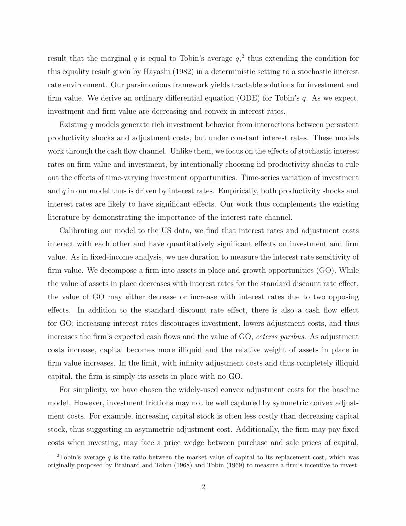
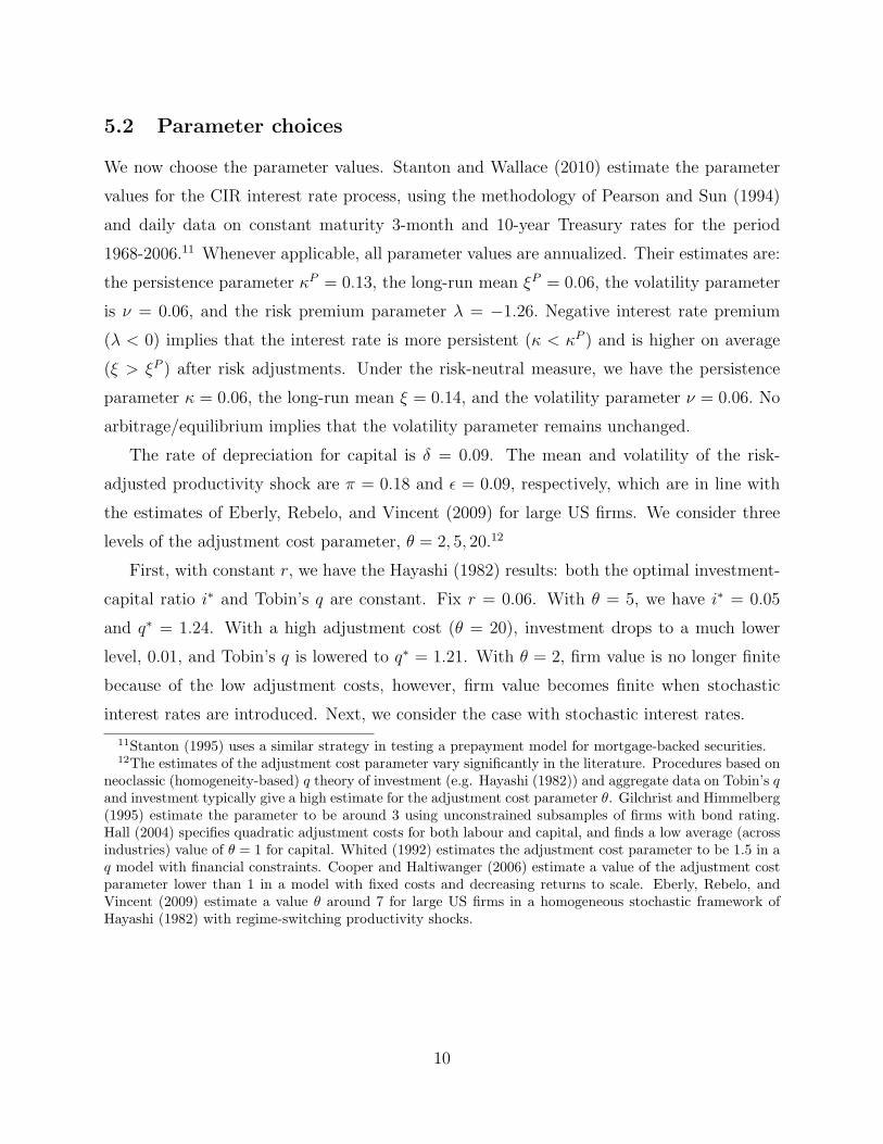
Figure 1: Tobin’s average q for various levels of adjustment costs

5.3 Investment, Tobin’s q, and duration

Figure 1 plots Tobin’s q(r) as a function of r for θ = 2, 5, 20. First, the lower the adjustment

cost parameter θ, the more productive capital and hence the higher Tobin’s q(r). Second,

q(r) is decreasing and convex in r. As we expect, firm value is quite sensitive to interest rate

movements. For example, with θ = 2, Tobin’s q at r = 0 is q(0) = 1.65, which is significantly

higher than q(0.06) = 1.10 at its long-run mean, ξP = 0.06. The firm loses about one-third

of its value (from 1.65 to 1.10) when the interest rate increases from 0 to 0.06.

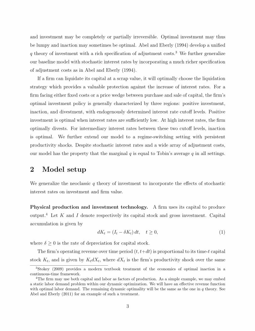
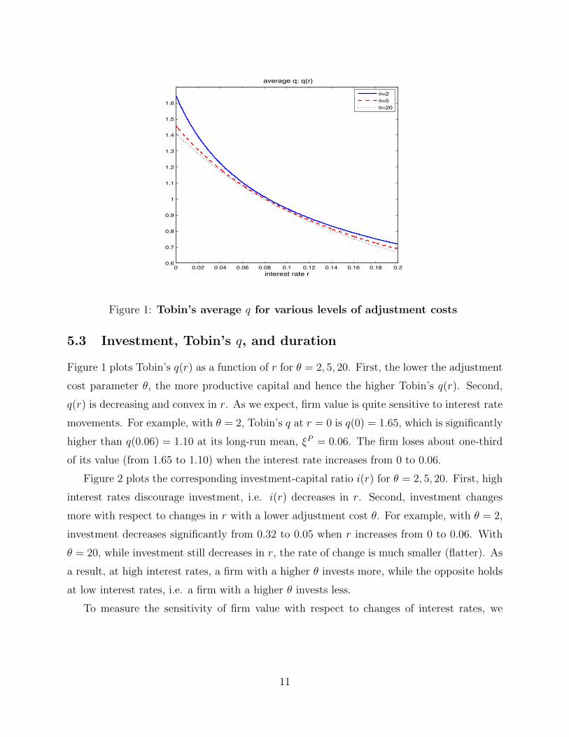
Figure 2 plots the corresponding investment-capital ratio i(r) for θ = 2, 5, 20. First, high

interest rates discourage investment, i.e. i(r) decreases in r. Second, investment changes

more with respect to changes in r with a lower adjustment cost θ. For example, with θ = 2,

investment decreases significantly from 0.32 to 0.05 when r increases from 0 to 0.06. With

θ = 20, while investment still decreases in r, the rate of change is much smaller (flatter). As

a result, at high interest rates, a firm with a higher θ invests more, while the opposite holds

at low interest rates, i.e. a firm with a higher θ invests less.

To measure the sensitivity of firm value with respect to changes of interest rates, we

11

0 0.02 0.04 0.06 0.08 0.1 0.12 0.14 0.16 0.18 0.20.2

0.1

0

0.1

0.2

0.3

0.4

interest rate r

investment capital ratio: i(r)

=2=5=20

Figure 2: The investment-capital ratio i(r) for various levels of adjustment costs

define duration for firm value as follows (motivated by duration in fixed-income analysis),

D(r) = − 1

V (K, r)

dV (K, r)

dr= −q

′(r)

q(r). (28)

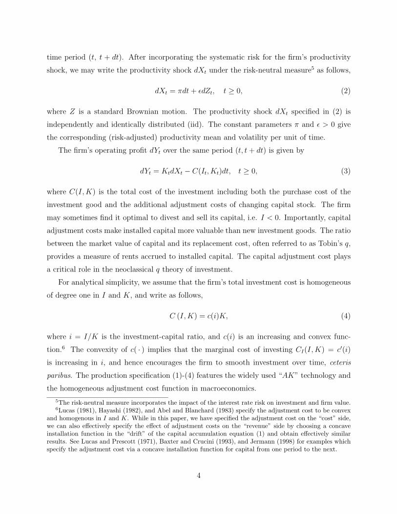
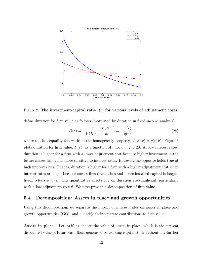
where the last equality follows from the homogeneity property, V (K, r) = q(r)K. Figure 3

plots duration for firm value, D(r), as a function of r for θ = 2, 5, 20. At low interest rates,

duration is higher for a firm with a lower adjustment cost because higher investment in the

future makes firm value more sensitive to interest rates. However, the opposite holds true at

high interest rates. That is, duration is higher for a firm with a higher adjustment cost when

interest rates are high, because such a firm divests less and hence installed capital is longer-

lived, ceteris paribus. The quantitative effects of r on duration are significant, particularly

with a low adjustment cost θ. We next provide a decomposition of firm value.

5.4 Decomposition: Assets in place and growth opportunities

Using this decomposition, we separate the impact of interest rates on assets in place and

growth opportunities (GO), and quantify their separate contributions to firm value.

Assets in place. Let A(K, r) denote the value of assets in place, which is the present

discounted value of future cash flows generated by existing capital stock without any further

12

0 0.02 0.04 0.06 0.08 0.1 0.12 0.14 0.16 0.18 0.22

3

4

5

6

7

8

9

10

11

interest rate r

duration: D(r)

=2=5=20

Figure 3: Duration for firm value, D(r), for various levels of adjustment costs

investment/divestment in the future, i.e. by permanently setting I = 0. Using the homo-

geneity property, we have A(K, r) = a(r) ·K. No gross investment (I = 0) implies that a(r)

solves the following linear ODE,

(r + δ) a(r) = π + µ(r)a′(r) +σ2(r)

2a′′(r) . (29)

As r →∞, assets are worthless, i.e. a(r)→ 0. At r = 0, we have π − δa(0) + κξa′(0) = 0 .

Intuitively, the value of assets in place (per unit of capital) for an infinitely-lived firm can

be viewed as a perpetual bond with a discount rate given by (r+ δ), the sum of interest rate

r and capital depreciation rate δ. Using the perpetual bond interpretation, the “effective”

coupon for this asset in place is the firm’s constant expected productivity π after the risk

adjustment (i.e. under the risk-neutral probability). The value of assets in place a(r) is

equal to Tobin’s q(r) if and only if no investment is the firm’s optimal decision making, i.e.

when the adjustment cost is infinity, θ =∞.

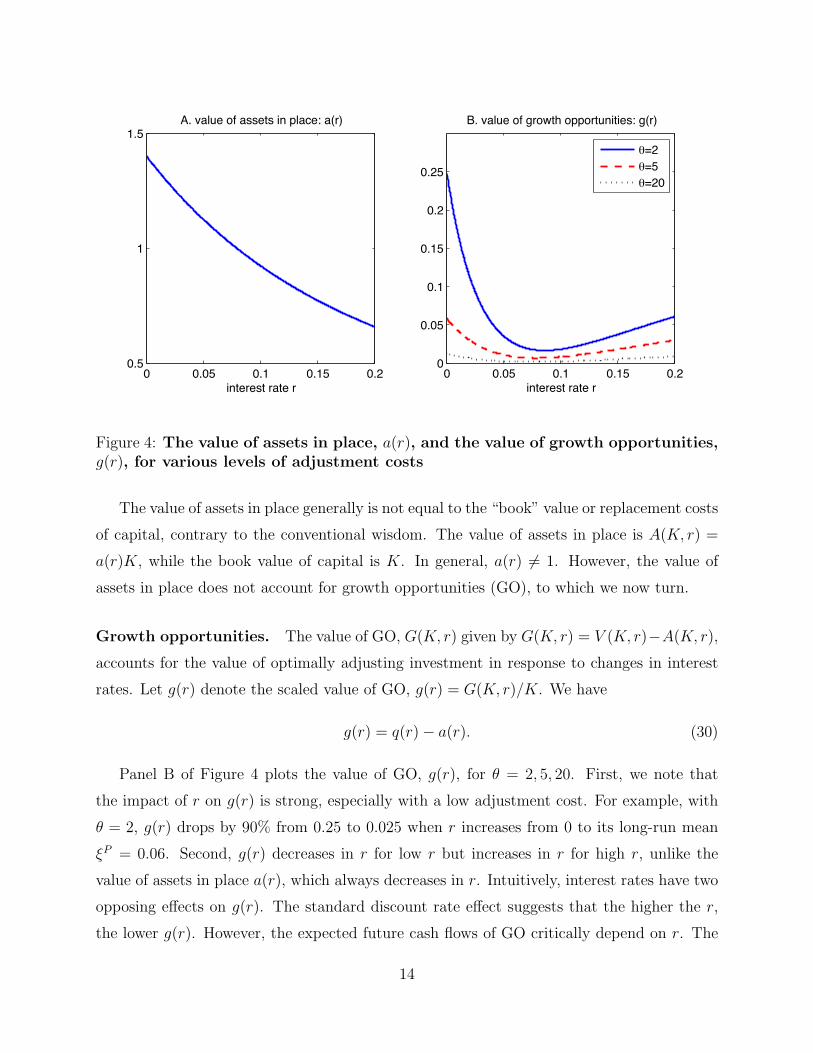
Panel A of Figure 4 plots the scaled value of assets in place, a(r). By definition, a(r) is

independent of GO and the adjustment cost parameter θ. By the perpetual bond interpreta-

tion, we know that a(r) is decreasing and convex in r. Quantitatively, a(r) accounts for a sig-

nificant fraction of firm value. For example, at its long-run mean ξP = 0.06, a(0.06) = 1.08,

which accounts for about 98% of total firm value, i.e. a(0.06)/q(0.06) = 0.98.

13

0 0.05 0.1 0.15 0.20.5

1

1.5A. value of assets in place: a(r)

interest rate r0 0.05 0.1 0.15 0.2

0

0.05

0.1

0.15

0.2

0.25

B. value of growth opportunities: g(r)

interest rate r

=2=5=20

Figure 4: The value of assets in place, a(r), and the value of growth opportunities,g(r), for various levels of adjustment costs

The value of assets in place generally is not equal to the “book” value or replacement costs

of capital, contrary to the conventional wisdom. The value of assets in place is A(K, r) =

a(r)K, while the book value of capital is K. In general, a(r) 6= 1. However, the value of

assets in place does not account for growth opportunities (GO), to which we now turn.

Growth opportunities. The value of GO, G(K, r) given by G(K, r) = V (K, r)−A(K, r),

accounts for the value of optimally adjusting investment in response to changes in interest

rates. Let g(r) denote the scaled value of GO, g(r) = G(K, r)/K. We have

g(r) = q(r)− a(r). (30)

Panel B of Figure 4 plots the value of GO, g(r), for θ = 2, 5, 20. First, we note that

the impact of r on g(r) is strong, especially with a low adjustment cost. For example, with

θ = 2, g(r) drops by 90% from 0.25 to 0.025 when r increases from 0 to its long-run mean

ξP = 0.06. Second, g(r) decreases in r for low r but increases in r for high r, unlike the

value of assets in place a(r), which always decreases in r. Intuitively, interest rates have two

opposing effects on g(r). The standard discount rate effect suggests that the higher the r,

the lower g(r). However, the expected future cash flows of GO critically depend on r. The

14

higher the interest rate r, the lower investment and hence the higher the expected cash flows,

which may be referred to as the cash flow effect of r. For sufficiently high r, the cash flow

effect overturns the discount rate effect, causing g(r) to increase in r. This cash flow effect

does not exist for a(r); its expected cash flow is π, a constant.

6 The value of the liquidation option

Capital often has an alternative use if deployed elsewhere. Empirically, there are significant

reallocation activities between firms as well as between sectors.13 We now extend the baseline

model by endowing the firm an option to liquidate its capital stock at any time; doing so

allows the firm to recover l per unit of capital where l > 0 is a constant. We show that the

optionality significantly influences firm investment and the value of capital.14 The following

theorem summarizes the main results.

Theorem 2 Tobin’s q, q(r), solves the ODE (15) subject to (16) and the following value-

matching and smooth-pasting boundary conditions

q(r∗) = l , (31)

q′(r∗) = 0 . (32)

The optimal investment strategy i(r) is given by (18).

The value-matching condition given in (31) states that q(r) is equal to its opportunity

cost l at liquidation. Because liquidation is optimal, we have the smooth-pasting condition

given in (32). Intuitively, at the endogenously chosen interest rate threshold level r∗ for

liquidation, the marginal effect of changes in r on Tobin’s q is zero. In summary, we obtain

Tobin’s q by solving the ODE (15) subject to the condition (16), and the two free boundary

conditions (31) and (32), which characterize the optimal liquidation boundary r∗.

Liquidation gives the firm an exit option to collect the opportunity cost of its capital.

This is an American-style option on interest rates. The firm effectively has a long position

13See Eisfeldt and Rampini (2006) and Eberly and Wang (2011) for equilibrium capital reallocation.14McDonald and Siegel (1986) and Dixit and Pindyck (1994) develop the real options approach of invest-

ment. Abel, Dixit, Eberly, and Pindyck (1996) integrate the option pricing approach into the q theory ofinvestment.

15

0 0.05 0.1 0.15 0.20.4

0.6

0.8

1

1.2

1.4

1.6

interest rate r

A. average q: q(r)

no liquidation optionwith liquidation option

0 0.05 0.1 0.15 0.20.2

0.1

0

0.1

0.2

0.3

0.4

interest rate r

B. investment capital ratio: i(r)

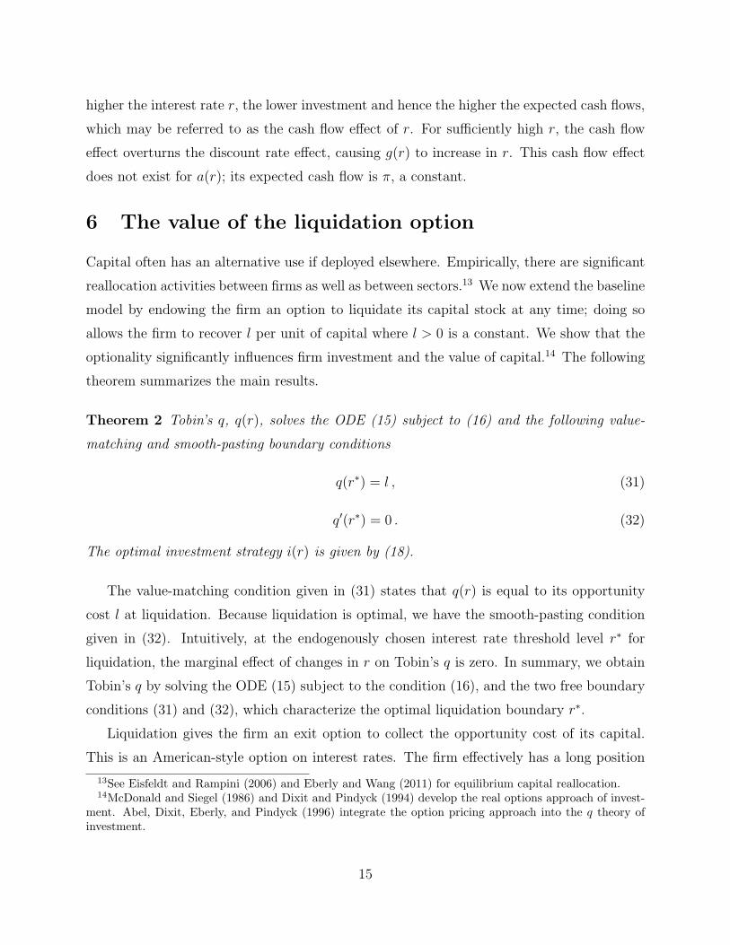
Figure 5: Tobin’s q and the investment-capital ratio i(r) with and without theliquidation option

in assets in place, a long position in growth opportunities, and also a long position in the

liquidation option. The liquidation option provides a protection for the value of capital

against the interest rate increase by putting a lower bound l for Tobin’s q.

For the quantitative exercise, we set the liquidation parameter value l = 0.9, i.e. the firm

recovers 90 cents on a dollar of the book value of capital upon liquidation (Hennessy and

Whited (2005)). We choose the adjustment cost parameter, θ = 2. Panels A and B of Figure

5 plot q(r) and i(r), respectively. In our example, the firm liquidates all its capital stock if

the interest rate is higher than r∗ = 0.14. Liquidating capital stock rather than operating

the firm as a going concern is optimal for sufficiently high interest rates, i.e. q(r) = l = 0.9

for r ≥ 0.14. Compared with the baseline case (with no liquidation option), the liquidation

option increases Tobin’s q and investment i(r) for all levels of r. The quantitative effects are

much stronger for interest rates closer to the liquidation boundary r∗ = 0.14 due to the fact

that the liquidation option is much closer to being in the money.

16

7 Asymmetry, price wedge, and fixed costs

7.1 Model setup

We extend the convex adjustment cost C(I,K) in our baseline model along three important

dimensions. Empirically, downward adjustments of capital stock are often more costly than

upward adjustments. We capture this feature by assuming that the firm incurs asymmetric

convex adjustment costs in investment (I > 0) and divestment (I < 0) regions. Hall (2001)

uses the asymmetric adjustment cost in his study of aggregate market valuation of capital

and investment. Zhang (2005) uses this asymmetric adjustment cost in studying investment-

based cross-sectional asset pricing.

Second, as in Abel and Eberly (1994, 1996), we assume a wedge between the purchase and

sale prices of capital, for example due to capital specificity and illiquidity premium. There

is much empirical work documenting the size of the wedge between the purchase and sale

prices. Arrow (1968) stated that “there will be many situations in which the sale of capital

goods cannot be accomplished at the same price as their purchase.” The wedge naturally

depends on the business cycles and market conditions.15 Let p+ and p− denote the respective

purchase and sale prices of capital. An economically sensible assumption is p+ ≥ p− ≥ 0

with an implied wedge p+ − p− .

Third, investment often incurs fixed costs. Fixed costs may capture investment indivisi-

bilities, increasing returns to the installation of new capital, and organizational restructuring

during periods of intensive investment. Additionally, fixed costs significantly improve the

empirical fit of the model with the micro data. Inaction becomes optimal in certain regions.

To ensure that the firm does not grow out of fixed costs, we assume that the fixed cost

is proportional to its capital stock. See Hall (2004), Cooper and Haltiwanger (2006), and

Riddick and Whited (2009) for the same size-dependent fixed cost assumption.

With the homogeneity property, we may write c(i) = C(I,K)/K. Following Abel and

15The estimates range from 0.6 to 1, depending on data sources, estimation methods, and model specifi-cations. See Pulvino (1998), Hennessy and Whited (2005), Cooper and Haltiwanger (2006), and Warusaw-itharana (2008), for example.

17

00 o

i

A. total scaled adjumtment costs: c(i)

0

1

i

B. marginal scaled adjumtment costs: c(i)

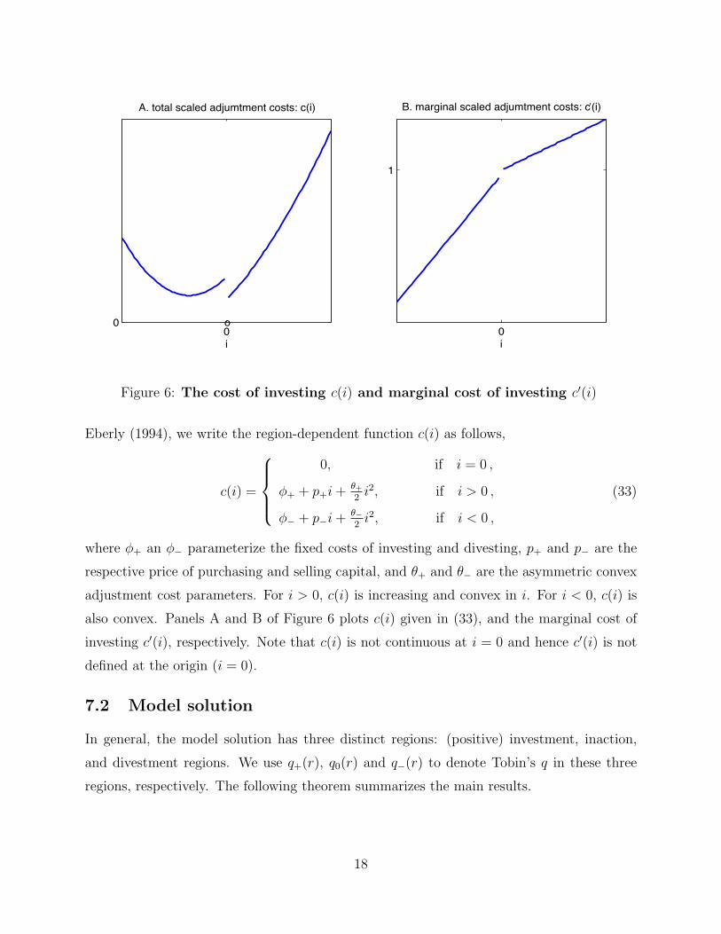
Figure 6: The cost of investing c(i) and marginal cost of investing c′(i)

Eberly (1994), we write the region-dependent function c(i) as follows,

c(i) =

0, if i = 0 ,

φ+ + p+i+ θ+2i2, if i > 0 ,

φ− + p−i+ θ−2i2, if i < 0 ,

(33)

where φ+ an φ− parameterize the fixed costs of investing and divesting, p+ and p− are the

respective price of purchasing and selling capital, and θ+ and θ− are the asymmetric convex

adjustment cost parameters. For i > 0, c(i) is increasing and convex in i. For i < 0, c(i) is

also convex. Panels A and B of Figure 6 plots c(i) given in (33), and the marginal cost of

investing c′(i), respectively. Note that c(i) is not continuous at i = 0 and hence c′(i) is not

defined at the origin (i = 0).

7.2 Model solution

In general, the model solution has three distinct regions: (positive) investment, inaction,

and divestment regions. We use q+(r), q0(r) and q−(r) to denote Tobin’s q in these three

regions, respectively. The following theorem summarizes the main results.

18

Theorem 3 Tobin’s q in investment, inaction, and divestment regions, q+(r), q0(r), and

q−(r), respectively, solve the following three linked ODEs,

(r + δ) q+(r) = π − φ+ +(q+(r)− p+)2

2θ+

+ µ(r)q′+(r) +σ2(r)

2q′′+(r), if r < r, (34)

(r + δ)q0(r) = π + µ(r)q′0(r) +σ2(r)

2q′′0(r), if r ≤ r ≤ r, (35)

(r + δ) q−(r) = π − φ− +(q−(r)− p−)2

2θ−+ µ(r)q′−(r) +

σ2(r)

2q′′−(r), if r > r . (36)

The endogenously determined cutoff interest rate levels for these three regions, r and r, satisfy

the following boundary conditions,

π − φ+ − δq+(0) +(q+(0)− p+)2

2θ+

+ κξq′+(0) = 0 , (37)

q+(r) = q0(r), q0(r) = q−(r) , (38)

q′+(r) = q′0(r), q′0(r) = q′−(r) , (39)

q′′+(r) = q′′0(r), q′′0(r) = q′′−(r) , (40)

limr→∞

q−(r) = 0 . (41)

The optimal investment-capital ratios, denoted as i+(r), i0(r), and i−(r), are given by

i+(r) =q+(r)− p+

θ+

, if r < r, (42)

i0(r) = 0, if r ≤ r ≤ r , (43)

i−(r) = −p− − q−(r)

θ−, if r > r . (44)

When r is sufficiently low (r ≤ r), the firm optimally chooses to invest, I > 0. Investment

is proportional to q+(r)−p+, the wedge between Tobin’s q and purchase price of capital, p+.

Tobin’s q in this region, q+(r), solves the ODE (34). Condition (37) gives the firm behavior

at r = 0. The right boundary r is endogenous. Tobin’s q at r, q+(r), satisfies the first set of

conditions in (38)-(40), i.e. q(r) is twice continuously differentiable at r.

Similarly, when r is sufficiently high (r ≥ r), the firm divests, I < 0. Divestment is

proportional to p− − q−(r), the wedge between the sale price of capital of capital, p−, and

Tobin’s q. Tobin’s q in the divestment region, q−(r), solves the ODE (36). Condition (41)

states that the firm is worthless as r →∞, the right boundary condition. The left boundary

for the divestment region r is endogenous. Tobin’s q at r, q−(r), satisfies the second set of

the conditions in (38)-(40), i.e. q(r) is twice continuously differentiable at r.

19

0 0.05 0.1 0.15 0.20.6

0.8

1

1.2

1.4

1.6

A. average q: q(r)

interest rate r

=2=5=20

0 0.05 0.1 0.15 0.20.2

0.1

0

0.1

0.2

0.3

0.4B. investment capital ratio: i(r)

interest rate r

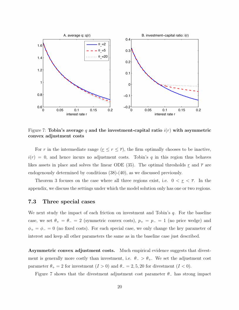
Figure 7: Tobin’s average q and the investment-capital ratio i(r) with asymmetricconvex adjustment costs

For r in the intermediate range (r ≤ r ≤ r), the firm optimally chooses to be inactive,

i(r) = 0, and hence incurs no adjustment costs. Tobin’s q in this region thus behaves

likes assets in place and solves the linear ODE (35). The optimal thresholds r and r are

endogenously determined by conditions (38)-(40), as we discussed previously.

Theorem 3 focuses on the case where all three regions exist, i.e. 0 < r < r. In the

appendix, we discuss the settings under which the model solution only has one or two regions.

7.3 Three special cases

We next study the impact of each friction on investment and Tobin’s q. For the baseline

case, we set θ+ = θ− = 2 (symmetric convex costs), p+ = p− = 1 (no price wedge) and

φ+ = φ− = 0 (no fixed costs). For each special case, we only change the key parameter of

interest and keep all other parameters the same as in the baseline case just described.

Asymmetric convex adjustment costs. Much empirical evidence suggests that divest-

ment is generally more costly than investment, i.e. θ− > θ+. We set the adjustment cost

parameter θ+ = 2 for investment (I > 0) and θ− = 2, 5, 20 for divestment (I < 0).

Figure 7 shows that the divestment adjustment cost parameter θ− has strong impact

20

0 0.05 0.1 0.15 0.20.6

0.8

1

1.2

1.4

1.6

A. average q: q(r)

interest rate r

p =1p =0.9p =0.8

0 0.05 0.1 0.15 0.20.2

0.1

0

0.1

0.2

0.3

0.4B. investment capital ratio: i(r)

interest rate r

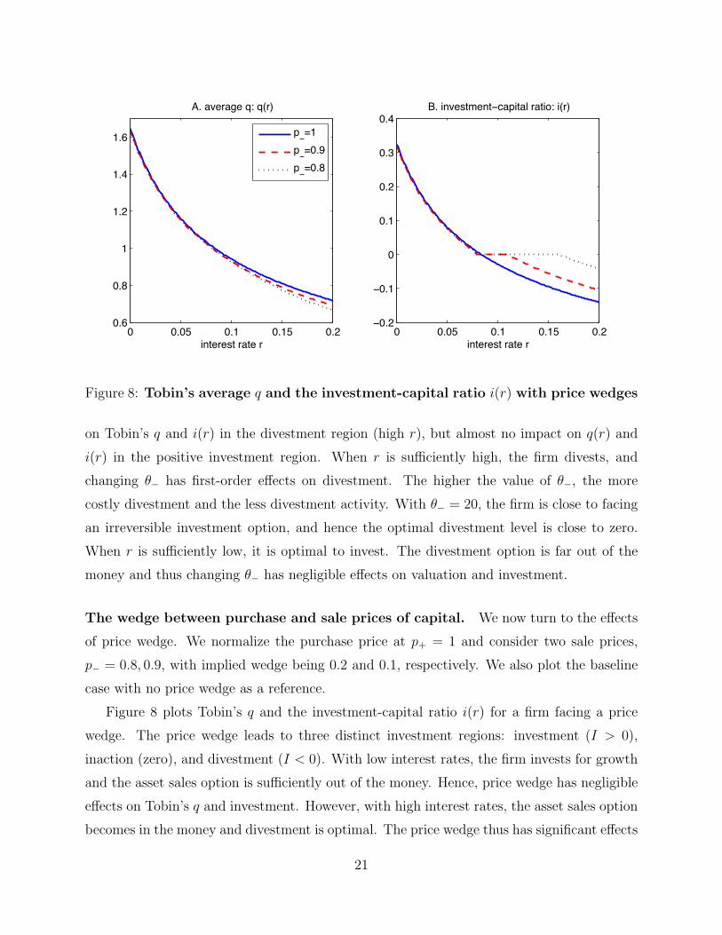
Figure 8: Tobin’s average q and the investment-capital ratio i(r) with price wedges

on Tobin’s q and i(r) in the divestment region (high r), but almost no impact on q(r) and

i(r) in the positive investment region. When r is sufficiently high, the firm divests, and

changing θ− has first-order effects on divestment. The higher the value of θ−, the more

costly divestment and the less divestment activity. With θ− = 20, the firm is close to facing

an irreversible investment option, and hence the optimal divestment level is close to zero.

When r is sufficiently low, it is optimal to invest. The divestment option is far out of the

money and thus changing θ− has negligible effects on valuation and investment.

The wedge between purchase and sale prices of capital. We now turn to the effects

of price wedge. We normalize the purchase price at p+ = 1 and consider two sale prices,

p− = 0.8, 0.9, with implied wedge being 0.2 and 0.1, respectively. We also plot the baseline

case with no price wedge as a reference.

Figure 8 plots Tobin’s q and the investment-capital ratio i(r) for a firm facing a price

wedge. The price wedge leads to three distinct investment regions: investment (I > 0),

inaction (zero), and divestment (I < 0). With low interest rates, the firm invests for growth

and the asset sales option is sufficiently out of the money. Hence, price wedge has negligible

effects on Tobin’s q and investment. However, with high interest rates, the asset sales option

becomes in the money and divestment is optimal. The price wedge thus has significant effects

21

0 0.05 0.1 0.15 0.20.6

0.8

1

1.2

1.4

1.6

A. average q: q(r)

interest rate r

!+=!−=0

!+=0,!−=0.01

!+=!−=0.01

0 0.1 0.2 0.3

−0.2

−0.1

0

0.1

0.2

0.3

B. investment−capital ratio: i(r)

interest rate r

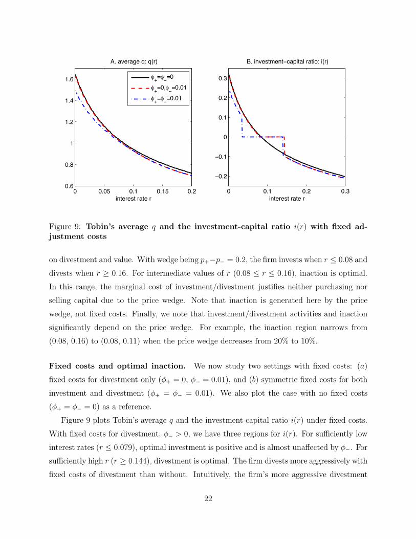
Figure 9: Tobin’s average q and the investment-capital ratio i(r) with fixed ad-justment costs

on divestment and value. With wedge being p+−p− = 0.2, the firm invests when r ≤ 0.08 and

divests when r ≥ 0.16. For intermediate values of r (0.08 ≤ r ≤ 0.16), inaction is optimal.

In this range, the marginal cost of investment/divestment justifies neither purchasing nor

selling capital due to the price wedge. Note that inaction is generated here by the price

wedge, not fixed costs. Finally, we note that investment/divestment activities and inaction

significantly depend on the price wedge. For example, the inaction region narrows from

(0.08, 0.16) to (0.08, 0.11) when the price wedge decreases from 20% to 10%.

Fixed costs and optimal inaction. We now study two settings with fixed costs: (a)

fixed costs for divestment only (φ+ = 0, φ− = 0.01), and (b) symmetric fixed costs for both

investment and divestment (φ+ = φ− = 0.01). We also plot the case with no fixed costs

(φ+ = φ− = 0) as a reference.

Figure 9 plots Tobin’s average q and the investment-capital ratio i(r) under fixed costs.

With fixed costs for divestment, φ− > 0, we have three regions for i(r). For sufficiently low

interest rates (r ≤ 0.079), optimal investment is positive and is almost unaffected by φ−. For

sufficiently high r (r ≥ 0.144), divestment is optimal. The firm divests more aggressively with

fixed costs of divestment than without. Intuitively, the firm’s more aggressive divestment

22

strategy economizes fixed costs of divestment. Additionally, fixed costs generates an inaction

region, 0.079 ≤ r ≤ 0.144. The impact of fixed costs of divestment is more significant on

Tobin’s q in medium to high r regions than in the low r region.

Now we incrementally introduce fixed costs for investment by changing φ+ from 0 to 0.01,

while holding φ− = 0.01. We have three distinct regions for i(r). For high r, r ≥ 0.14, the

firm divests. Tobin’s q and i(r) in this region remain almost unchanged by φ+. For low r,

r ≤ 0.035, the firm invests less with φ+ = 0.01 than with φ+ = 0.

Introducing the fixed costs φ+ discourages investment, lowers Tobin’s q, shifts the inaction

region to the left, and widens the inaction region. The lower the interest rate, the stronger

the effects of φ+ on Tobin’s q, investment, and the inaction region.

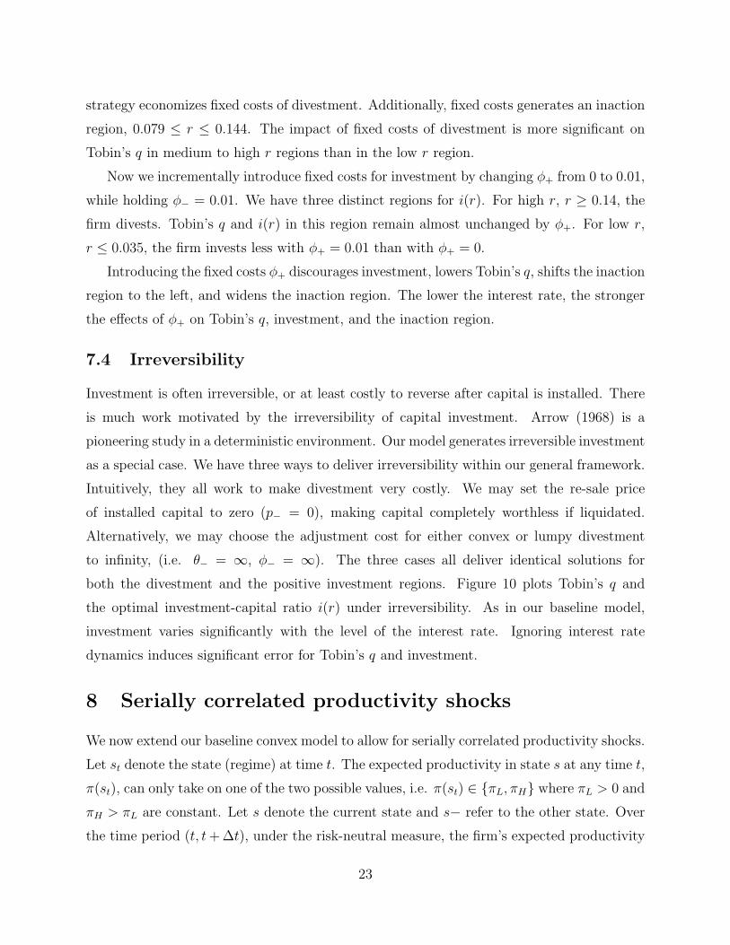
7.4 Irreversibility

Investment is often irreversible, or at least costly to reverse after capital is installed. There

is much work motivated by the irreversibility of capital investment. Arrow (1968) is a

pioneering study in a deterministic environment. Our model generates irreversible investment

as a special case. We have three ways to deliver irreversibility within our general framework.

Intuitively, they all work to make divestment very costly. We may set the re-sale price

of installed capital to zero (p− = 0), making capital completely worthless if liquidated.

Alternatively, we may choose the adjustment cost for either convex or lumpy divestment

to infinity, (i.e. θ− = ∞, φ− = ∞). The three cases all deliver identical solutions for

both the divestment and the positive investment regions. Figure 10 plots Tobin’s q and

the optimal investment-capital ratio i(r) under irreversibility. As in our baseline model,

investment varies significantly with the level of the interest rate. Ignoring interest rate

dynamics induces significant error for Tobin’s q and investment.

8 Serially correlated productivity shocks

We now extend our baseline convex model to allow for serially correlated productivity shocks.

Let st denote the state (regime) at time t. The expected productivity in state s at any time t,

π(st), can only take on one of the two possible values, i.e. π(st) ∈ {πL, πH} where πL > 0 and

πH > πL are constant. Let s denote the current state and s− refer to the other state. Over

the time period (t, t+ ∆t), under the risk-neutral measure, the firm’s expected productivity

23

0 0.05 0.1 0.15 0.20.6

0.8

1

1.2

1.4

1.6

interest rate r

A. average q: q(r)

p =0

==

0 0.05 0.1 0.15 0.20.05

0

0.05

0.1

0.15

0.2

0.25

0.3

B. investment capital ratio: i(r)

interest rate r

Figure 10: Tobin’s average q and the investment-capital ratio i(r) when investmentis irreversible

changes from πs to πs− with probability ζs∆t, and stays unchanged at πs with the remaining

probability 1 − ζs∆t. The change of the regime may be recurrent. That is, the transition

intensities from either state, ζ1 and ζ2, are strictly positive. The incremental productivity

shock dX after risk adjustments (under the risk neutral measure) is given by

dXt = π(st−)dt+ ε(st−)dZt , t ≥ 0 . (45)

The firm’s operating profit dYt over the same period (t, t + dt) is also given by (3) as in

the baseline model. The homogeneity property continues to hold. The following theorem

summarizes the main results.

Theorem 4 Tobin’s q in two regimes, qH(r) and qL(r), solves the following linked ODEs:

(r + δ) qs(r) = πs+(qs(r)− 1)2

2θ+µ(r)q′s(r)+

σ2(r)

2q′′s (r)+ζs(qs−(r)−qs(r)), s = H, L, (46)

subject to the following boundary conditions,

πs − δqs(0) +(qs(0)− 1)2

2θ+ κξq′s(0) + ζs(qs−(0)− qs(0)) = 0 , (47)

limr→∞

qs(r) = 0 . (48)

24

0 0.05 0.1 0.15 0.20.4

0.6

0.8

1

1.2

1.4

1.6

interest rate r

A. average q: q(r)

qL(r)qH(r)

0 0.05 0.1 0.15 0.2

0.1

0.05

0

0.05

0.1

0.15

interest rate r

B. investment capital ratio: i(r)

iL(r)iH(r)

Figure 11: Tobin’s average q and the investment-capital ratio i(r) with seriallycorrelated productivity shocks

The optimal investment-capital ratios in two regimes iH(r) and iL(r) are given by

is(r) =qs(r)− 1

θ, s = H, L. (49)

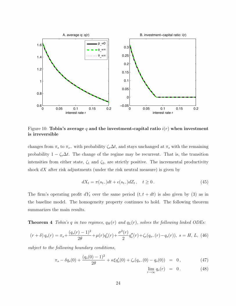
Figure 11 plots Tobin’s average q and the investment-capital ratio i(r) for both the

high- and the low-productivity regimes. We choose the expected (risk-neutral) productivity,

πH = 0.2 and πL = 0.14, set the (risk-neutral) transition intensities at ζL = ζH = 0.03. The

expected productivity has first-order effects on firm value and investment; both qH(r) and

iH(r) are significantly larger than qL(r) and iL(r), respectively. Additionally, both qH(r) and

qL(r) are decreasing and convex as in the baseline model. Our model with serially correlated

productivity shocks can be extended to allow for richer adjustment cost frictions such as

the price wedge and fixed costs as we have done in the previous section, and multiple-state

Markov chain processes for productivity shocks.

9 Conclusion

A fundamental determinant of investment and value is interest rates, which change stochas-

tically over time and have time-varying risk premia. Existing q models focus on capital

25

illiquidity induced by adjustment costs and assume constant interest rates. We recognize

the importance of stochastic interest rates and incorporate a widely-used CIR term structure

model into the neoclassic q theory of investment (Hayashi (1982) and Abel and Eberly (1994,

1996)). We capture the impact of interest rate mean reversion, volatility, and risk premia

on investment and the value of capital. We provide analytical solutions for Tobin’s q as a

function of the interest rate by deriving and solving an ODE. As in fixed-income analysis, we

use duration to measure the interest rate sensitivity of firm value, and find that the duration

decreases and varies significantly with interest rates.

We decompose a firm into its assets in place and growth opportunities (GO). While the

value of assets in place decreases with the interest rate, the value of GO may either increase

or decrease with the interest rate. When the firm has an option to endogenously liquidate its

capital at a scrap value, it will optimally exercise this exit option (a put option on interest

rates) to protect itself against the increase of interest rates.

Motivated by empirical evidence on lumpy and partially irreversible investment, we gen-

eralize our model with convex adjustment costs to incorporate asymmetric adjustment costs,

a price wedge between purchasing and selling capital, fixed costs, and irreversibility. We find

that the optimal inaction region critically depends on the interest rate and is quantitatively

important. We further extend our model to incorporate persistent productivity shocks. We

show that marginal q is equal to average q in our framework despite stochastic interest rates

and persistent productivity shocks, thus extending the equality result of Hayashi (1982)

obtained under constant interest rates and deterministic investment opportunities.

For simplicity, we have chosen a one-factor term structure model for interest rates. Much

empirical evidence shows that term structure is much richer (see Piazzesi (2010) for a survey).

Investment and the value of capital naturally depend on various underlying factors. Finally,

we may extend our homogeneous framework to incorporate decreasing returns to scale and

a more general non-homogenous adjustment cost specification, either of which will generate

a wedge between marginal q and average q. We leave these economically motivated but

technically involved extensions for future research.

26

Appendices

A Sketch of technical details

For Theorem 1. Using the homogeneity property of V (K, r), we conjecture that V (K, r) =

Kq(r) as in (13), which implies VK(K, r) = q(r), Vr(K, r) = Kq′(r), and Vrr(K, r) = Kq′′(r).

Substituting these into the PDE (9) for V (K, r) and simplifying, we obtain

rq(r) = maxi

(π − c(i)) + (i− δ) q(r) + µ(r)q′(r) +σ2(r)

2q′′(r). (A.1)

Using the FOC (10) for investment I and simplifying, we obtain (18) for the optimal i(r).

Substituting the optimal i(r) given by (18) into the ODE (A.1), we have the ODE (15) for

q(r). Evaluating the ODE (15) at r = 0 gives the boundary condition (16) at r = 0. Finally,

V (K, r) approaches zero as r →∞, which implies limr→∞ q(r) = 0 given in (17).

For Proposition 1. With constant interest rates, we may simplify (A.1) as follows,

rq(r) = maxi

(π − c(i)) + (i− δ) q(r). (A.2)

Substituting the optimal i into (A.2) and using economic intuition (higher productivity leads

to higher investment and value), we explicitly solve i = I/K, which is given by (21).

The value of assets in place, a(r). For A(K, r), we have the following HJB equation:

rA(K, r) = πK − δKAK(K, r) + µ(r)Ar(K, r) +σ2(r)

2Arr(K, r) . (A.3)

Using A(K, r) = K · a (r) and substituting it into (A.3), we obtain the ODE(29) for a(r).

The value of assets in place A(K, r) vanishes as r → ∞, i.e. limr→∞A(K, r) = 0, which

implies limr→∞ a(r) = 0. Equation (29) implies that the natural boundary condition at r = 0

should be π − δa(0) + κξa′(0) = 0.

For Theorem 2. With a liquidation option, the firm optimally exercises its option so

that V (K, r) satisfies the value matching condition V (K, r∗) = lK, and the smooth pasting

condition Vr(K, r∗) = 0. With V (K, r) = q(r)K, we obtain q(r∗) = l and q′(r∗) = 0, given

by (31) and (32), respectively.

27

For Theorem 3. With homogeneity property, we conjecture that there are three re-

gions (positive, zero, and negative investment regions), separated by two endogenous cutoff

interest-rate levels r and r. Firm value in the three regions can be written as follows,

V (K, r) =

K · q− (r) , if r > r,K · q0 (r) , if r ≤ r ≤ r,K · q+ (r) , if r < r,

(A.4)

Importantly, at r and r, V (K, r) satisfies value-matching, smooth-pasting, and super contact

conditions, which imply (38), (39), and (40), respectively. Note that (37) is the natural

boundary condition at r = 0 and (41) reflects that firm value vanishes as r → ∞. Other

details are essentially the same as those in Theorem 1.

When the fixed cost for investment φ+ is sufficiently large, there is no investment region,

i.e. r = 0. Additionally, the condition at r = 0, (37), is replaced by the following condition,

π − δq0(0) + κξq′0(0) = 0 . (A.5)

In sum, for the case with inaction and divestment regions, the solution is given by the linked

ODEs (35)-(36) subject to (A.5), the free-boundary conditions for the endogenous threshold

r given as the second set of conditions in (38)-(40), and the limit condition (41).

Similarly, if the cost of divestment φ− is sufficiently high, the firm has no divestment

region, i.e. r =∞. The model solution is given by the linked ODEs (34)-(35) subject to (37),

the free-boundary conditions for r given as the first set of conditions, and limr→∞ q0(r) = 0 .

For Theorem 4. Firm value in the low and high productivity regimes, V (K, r, πL) and

V (K, r, πH), jointly solve the following coupled HJB equations:

rV (K, r, πL) = maxI

(πLK − C(I,K)) + (I − δK)VK(K, r, πL) + µ(r)Vr(K, r, πL)

+σ2(r)

2Vrr(K, r, πL) + ζL(V (K, r, πH)− V (K, r, πL)). (A.6)

rV (K, r, πH) = maxI

(πHK − C(I,K)) + (I − δK)VK(K, r, πH) + µ(r)Vr(K, r, πH)

+σ2(r)

2Vrr(K, r, πH) + ζH(V (K, r, πL)− V (K, r, πH)). (A.7)

Using the homogeneity property, we conjecture V (K, r, πs) = K · qs (r), for s = H,L. The

remaining details are essentially the same as those for Theorem 1.

28

References

Abel, A. B., 1983, “Optimal investment under uncertainty,” American Economic Review,

73, 228-233.

Abel, A. B., and O. J. Blanchard, 1983, “An intertemporal model of saving and invest-

ment,”Econometrica, 51, 675-692.

Abel, A. B., A. K. Dixit, J. C. Eberly and R. S. Pindyck, 1996, “Options, the value of

capital, and investment,” Quarterly Journal of Economics, 111, 753-777.

Abel, A. B., and J. C. Eberly, 1994, “A unified model of investment under uncertainty,”

American Economic Review, 84, 1369-1384.

Abel, A. B., and J. C. Eberly, 1996, “Optimal investment with costly reversibility,” Review

of Economic Studies, 63, 581-593.

Abel, A. B., and J. C. Eberly, 2011, “How Q and cash flow affect investment without

frictions: An analytic explanation,” Review of Economic Studies, forthcoming.

Arrow, K. J., 1968, “Optimal capital policy with irreversible investment,” in J. N. Wolfe,

ed., Value, capital and growth. Papers in honour of Sir John Hicks. Edinburgh:

Edinburge University Press, 1-19.

Baxter, M., and M. J. Crucini, 1993, “Explaining saving-investment correlations,”American

Economic Review, 83, 416-36.

Brainard, W. C., and J. Tobin, 1968, “Pitfalls in Financial Model-Building,”American

Economic Review, 58, 99-122.

Caballero, R. J., 1999, “Aggregate investment,”in J. B. Taylor, and M. Woodford (ed.),

Handbook of Macroeconomics, vol. 1 of Handbook of Macroeconomics, Ch. 12, pp.

813-862, Elsevier.

Cooper, R. S. and J. C. Haltiwanger, 2006, “On the nature of capital adjustment costs,”

Review of Economic Studies, 73, 611-633.

29

Cox, J. C., J. E. Ingersoll, Jr., and S. A. Ross, 1985, “A theory of term structure of interest

rates,” Econometrica, 53, 385-408.

Dai, Q., and K. Singleton, 2000, “Specification Analysis of Affine Term Structure Mod-

els,”Journal of Finance, 55, 1943-1978.

Dixit, A. K., and R. S. Pindyck, 1994, Investment Under Uncertainty, Princeton University

Press, Princeton, NJ.

Duffie, J. D., 2002, Dynamic Asset Pricing Theory, Princeton University Press, Princeton,

NJ.

Duffie, J. D., and R. Kan, 1996, “A yield-factor model of interest rates,”Mathematical

Finance, 6, 379-406.

Eberly, J. C., S. Rebelo, and N. Vincent, 2009, “Investment and value: A neoclassical

benchmark,” working paper, Northwestern University.

Eblery, J. C., and N. Wang, 2011, “Reallocating and pricing illiquid capital: Two productive

trees,” working paper, Columbia University and Northwestern University.

Eisfeldt, A., L, and A. A. Rampini, 2006, “Capital reallocation and liquidity,”Journal of

Monetary Economics, 53, 369-399.

Gilchrist, S., and C. P. Himmelberg, 1995, “Evidence on the role of cash flow for investment

”Journal of Monetary Economics, 36, 541-572.

Hall, R. E., 2001, “The stock market and capital accumulation,”American Economic Re-

view, 91, 1185-1202.

Hall, R. E., 2004, “Measuring factor adjustment costs,” Quarterly Journal of Economics,

119, 899-927.

Hayashi, F., 1982, “Tobin’s marginal Q and average Q: A neoclassical interpretation,”

Econometrica, 50, 215-224.

Hennessy, C. A., and T. M. Whited, 2005, “Debt Dynamics,”Journal of Finance, 60, 1129-

1165.

30

Jermann, U. J., 1998, “Asset Pricing in Production Economies,” Journal of Monetary

Economics, 257-275.

Jorgenson, D. W., 1963, “Capital Theory and Investment Behavior,”American Economic

Review, 53(2), 247-59.

Lucas, R. E., Jr., 1981, “Optimal investment with rational expectation,”in R. E. Lucas, Jr.,

and T. J. Sargent, Rational expectations and economic behavior, Vol I., Minneapolis:

University of Minnesota Press, 55-66.

Lucas, R. E., Jr., and E. C. Prescott, 1971, “Investment Under Uncertainty,”Econometrica,

39, 659-681.

Ljungqvist, L., and T. J. Sargent, 2004, Recursive Macroeconomic Theory, MIT Press,

Cambridge, MA.

McDonald, R., and Siegel, D., 1986, “The value of waiting to invest,”Quarterly Journal of

Economics, 101, 707728.

Mussa, M., 1977, “External and Internal Adjustment Costs and the Theory of Aggregate

and Firm Investment,”Economica, 44, 163-178.

Pearson, N. D., and T. S. Sun,1994, “Exploiting the conditional density in estimating the

term structure: An application to the Cox, Ingersoll, and Ross model,”Journal of

Finance, 54, 1279-1304.

Piazzesi, M., 2010, “Affine Term Structure Models,”in Y. Ait-Sahalia and L. P. Hansen

(eds.), Handbook of Financial Econometrics, Elsevier.

Pulvino, T. C., 1998, “Do Asset Fire Sales Exist? An Empirical Investigation of Commercial

Aircraft Transactions,”Journal of Finance, 53, 939-978.

Riddick, L. A., and T. M. Whited, 2009, “The Corporate Propensity to Save,”Journal of

Finance, 64, 1729-1766.

Stanton, R. 1995, “Rational Prepayment and the Value of MortgageBacked Securities,”Review

of Financial Studies, 8, 677-708.

31

Stanton, R., and N. Wallace, 2010, “CMBS Subordination, Ratings inflation, and the Crisis

of 2007-2009,”Haas School of Business, working paper.

Stokey, N. L., 2009, The Economics of Inaction: Stochastic Control Models with Fixed

Costs, Princeton University Press, Princeton, NJ.

Tobin, J., 1969, “A General Equilibrium Approach to Monetary Theory,”Journal of Money,

Credit and Banking, 1, 15-29.

Vasicek, O., 1977, “An equilibrium characterization of the term structure,”Journal of Fi-

nancial Economics, 5 (2), 177-188.

Warusawitharana, M., 2008, “Corporate asset purchases and sales: Theory and evidence,”Journal

of Financial Economics, 87, 471-497.

Whited, T. M., 1992, “Debt, Liquidity Constraints, and Corporate Investment: Evidence

from Panel Data,”Journal of Finance, 47, 1425-60.

Zhang, L., 2005, “The Value Premium,”Journal of Finance, 60, 67-104.

32