Stochastic Model Predictive Control for Building Climate Control

1198 IEEE TRANSACTIONS ON CONTROL SYSTEMS TECHNOLOGY, VOL. 22, NO. 3, MAY 2014

Stochastic Model Predictive Control for Building Climate ControlFrauke Oldewurtel, Member, IEEE, Colin Neil Jones, Member, IEEE,

Alessandra Parisio, Member, IEEE, and Manfred Morari, Fellow, IEEE

Abstract— In this brief paper, a Stochastic Model PredictiveControl formulation tractable for large-scale systems is devel-oped. The proposed formulation combines the use of AffineDisturbance Feedback, a formulation successfully applied inrobust control, with a deterministic reformulation of chance con-straints. A novel approximation of the resulting stochastic finitehorizon optimal control problem targeted at building climatecontrol is introduced to ensure computational tractability. Thiswork provides a systematic approach toward finding a controlformulation which is shown to be useful for the applicationdomain of building climate control. The analysis follows twosteps: 1) a small-scale example reflecting the basic behavior ofa building, but being simple enough for providing insight intothe behavior of the considered approaches, is used to choosea suitable formulation; and 2) the chosen formulation is thenfurther analyzed on a large-scale example from the projectOptiControl, where people from industry and other researchinstitutions worked together to create building models for realisticcontroller comparison. The proposed Stochastic Model PredictiveControl formulation is compared with a theoretical benchmarkand shown to outperform current control practice for buildings.

Index Terms— Affine disturbance feedback (ADF), buildingclimate control, chance constraints, Stochastic model predictivecontrol (SMPC).

I. INTRODUCTION

THIS brief paper is concerned with solving a Model Pre-dictive Control (MPC) problem for the class of discrete-

time linear systems subject to stochastic disturbances. Theaim is to provide a method for efficiently finding controlpolicies given a set of polytopic input constraints and chanceconstraints on the state, which is computationally tractable tobe applicable to large-scale systems.

One example of a control problem, which naturally leadsto chance constraints and which is the primary motivationfor this brief paper, originates from building climate control.In European building standards, it is required that the roomtemperature is kept within a comfort range with a predefinedprobability [1]. The control problem is to minimize energywhile satisfying this chance constraint. MPC for building

Manuscript received April 20, 2012; revised May 2, 2013; accepted June21, 2013. Manuscript received in final form July 1, 2013. Date of publicationAugust 1, 2013; date of current version April 17, 2014. Recommended byAssociate Editor E. Kerrigan.

F. Oldewurtel is with the Power Systems Laboratory, ETH Zurich, Zurich8092, Switzerland (e-mail: [email protected]).

C. N. Jones is with the Automatic Control Laboratory, EPFL Lausanne,Lausanne CH-1015, Switzerland (e-mail: [email protected]).

A. Parisio is with the Automatic Control Laboratory, KTH Stockholm,Stockholm SE-100 44, Sweden (e-mail: [email protected]).

M. Morari is with the Automatic Control Laboratory, ETH Zurich, Zurich8092, Switzerland (e-mail: [email protected]).

Color versions of one or more of the figures in this paper are availableonline at http://ieeexplore.ieee.org.

Digital Object Identifier 10.1109/TCST.2013.2272178

climate control using weather and occupancy predictionshas been addressed in several works, see [2]–[10] or theweb site of the OptiControl project [11] and the referencestherein.

This brief paper provides a systematic approach to addressthe uncertainty in weather predictions, formulate chance con-straints, and obtain a suitable control formulation for thebuilding application domain. A deterministic reformulation ofthe chance constraints is combined with affine disturbancefeedback, a parameterization of the control inputs, to obtaina tractable formulation of stochastic MPC, applicable alsoto large-scale systems such as buildings. By using affinedisturbance feedback and by exploiting the fact that comfortviolations are allowed from time to time with the chanceconstraints, the conservatism of traditional robust solutions isreduced. The presented material is an extension to the ideasproposed in [12] and offers a comparison and analysis ofdifferent formulations. The chosen formulation is assessed ona large-scale building example from the OptiControl projectand shown to outperform current control practice.

A. Dealing With Uncertainty

In the presence of uncertainties, it is generally preferableinstead of finding the optimal open-loop input sequence tooptimize over closed-loop policies, i.e., to assume that thepredicted control inputs at each time step are a state feedbackcontroller (or, equivalently, a disturbance feedback controller).Hence the predicted control input at time t is formulated as afunction of the states from now up to time t , or, equivalently,as a function of the disturbances that have happened from nowup to time t−1.

Finding optimal closed-loop policies involves the opti-mization over an infinite-dimensional function space and isnot tractable except for very special cases. It is thereforea common procedure to restrict the optimization to a finitedimensional subspace of the policies, i.e., to choose a controlparameterization and optimize over its parameters.

A popular approach is to use a fixed feedback gain[13]–[15], where the control inputs u are parameterized as u =K x +c, with K being some stabilizing linear feedback controllaws and the perturbation sequence c being the optimizationvariable. A natural improvement is to simultaneously optimizeover both the feedback gain and the perturbation sequence.However, in general, with this approach, the predicted stateand input sequences are nonlinear functions of the sequenceof state feedback gains and hence it results in a nonconvex setof feasible decision variables.

Inspired from the results in optimization theoryon robust optimization problems, in particular, on

1063-6536 © 2013 IEEE. Personal use is permitted, but republication/redistribution requires IEEE permission.

See http://www.ieee.org/publications_standards/publications/rights/index.html for more information.

OLDEWURTEL et al.: STOCHASTIC MPC FOR BUILDING CLIMATE CONTROL 1199

so-called adjustable robust counterpart [16] problems,Löfberg [17] and van Hessem and Bosgra [18]propose to parameterize the control inputs to be affinefunctions of the disturbances, which leads to a convex set offeasible decision variables. This affine disturbance feedbackparameterization is shown to be equivalent to the affine statefeedback parameterization in [19]. A more general approachis that of nonlinear disturbance feedback, where the decisionvariables are the coefficients of a linear combination ofnonlinear basis functions of the disturbance [20]. In thiswork, it is investigated how the use of Affine DisturbanceFeedback can be extended to the stochastic setting.

B. Formulation of Chance Constraints

For problems, where it is not necessary to apply hardconstraints, the use of chance constraints can be beneficialbecause it allows to formulate explicitly the tradeoff betweenperformance and constraint satisfaction [21]. Let x ∈ R

nx bethe system state, w ∈ R

nw the disturbance, and ξ ∈ Rr×nx ,

δ ∈ Rr×nw , as well as ε ∈ R

r be constants. Chance constraintsare assumed to be of the form

P[ξi x + δiw ≤ εi ] ≥ 1 − βi , i = 1, . . . , r (1)

where βi ∈ (0, 1) is the probability of constraint violation.Chance constraints were first introduced by [22] and havebeen studied extensively in the field of stochastic programming[23]–[25]. The standard approach in stochastic programmingis to consider discrete distributions and then to look at differentscenarios, which can be computationally very demanding.Various approaches have been proposed for stochastic MPC,see [26]–[28] and the references therein.

C. Notation

The real number set is denoted by R, the set of nonnegativeintegers by N (N+ := N\{0}), the set of consecutive non-negative integers { j, . . . , k} by N

kj . Denote by In ∈ {0, 1}n×n

the identity matrix, by 0n×m ∈ {0}n×m the zero matrix and by 0without subscript the zero matrix with dimension deemedobvious by context. ⊗ denotes the Kronecker product. Letvec(x, y) := [xT yT ]T denote the vertical concatenation ofvectors x and y and let vec(A) be the vertical concatenationof the columns of matrix A, i.e., if A = [a1, . . . , an], thenvec(A) = vec(a1, . . . , an).

II. PROBLEM SETTING

Consider the following discrete-time LTI system:

x+ = Ax + Bu + Ew (2)

with system state x ∈ Rnx , control input u ∈ R

nu , andstochastic disturbance w ∈ R

nw .Assumption 1: (A, B) is stabilizable and at each sample

instant a measurement of the state is available.Assumption 2: The disturbance is assumed to be inde-

pendent and identically distributed (i.i.d.) and to follow amultivariate normal distribution, w ∼ N (0nw×1, Inw ).

In the following, predictions about the system’s evolutionover a finite planning horizon are used to define suitablecontrol policies. Consider the prediction horizon N ∈ N+ anddefine

x :=[x T

0 . . . x TN

]T ∈ R(N+1)nx

u :=[uT

0 . . . uTN−1

]T ∈ RNnu

w :=[wT

0 . . . wTN−1

]T ∈ RNnw (3)

where x0 denotes the current measured value of the state andxk+1 := Axk + Buk + Ewk , k ∈ N

N−10 denotes the predictions

of the state after k time instants into the future. Let furthermoreprediction dynamics matrices A, B, and E be such that

x = Ax0 + Bu + Ew. (4)

Polytopic constraints on inputs u and chance constraints onstates x over the prediction horizon N are given as

Su ≤ s (5)

P[G j x ≤ g j

] ≥ 1 − αx, j ∀ j ∈ Nr(N+1)1 (6)

where S ∈ Rq N×nu N , s ∈ R

q N , G ∈ Rr(N+1)×nx (N+1), g ∈

Rr(N+1), and αx, j ∈ (0, 0.5] denotes the probability level of

constraint violation for row j of the constraints on x.Remark 1: αx, j is restricted to be in (0, 0.5] as it can then

be reformulated into a second order cone (SOC) constraint.x0 is measured, however, the predicted states x1, . . . , xN areuncertain. To address this uncertainty in the MPC formulation,consider for predicted control inputs u1, . . . , uN a causalstate feedback controller, or equivalently, a causal disturbancefeedback controller

uk = φk(x1, . . . , xk) = μk(w0, . . . , wk−1). (7)

Remark 2: The state feedback controller is called causal as itstrictly depends on the states that have already been realized.It is equivalent to consider a disturbance feedback controller,as the disturbances can be straightforwardly computed withgiven states and known inputs.

The aim is to solve the following stochastic finite horizonoptimal control problem (SFHOCP).

Problem 1 (SFHOCP):

minu

E

[N−1∑k=0

lk(xk, uk) + lN (xN )

]

s.t. Su ≤ s

P[G j x ≤ g j

] ≥ 1 − αx, j ∀ j ∈ Nr(N+1)1

x = Ax0 + Bu + Ew

w ∼ N (0nw N×1, Inw N )

uk = μk(w0, . . . , wk−1)

for some stage cost lk(xk, uk) and some terminal cost lN (xN ).Note that in Problem I, the aim is not to find an optimal controlinput sequence, but to find an optimal control policy as definedin (7) taking into account that there is recourse/ feedbackat every future stage/ time step. This SFHOCP cannot bereadily solved, as it involves the optimization over an infinite-dimensional function space. This problem is tackled in this


brief paper by restricting the policies to a finite-dimensionalsubspace. Furthermore, the above problem involves chanceconstraints that are to be reformulated so that they can beefficiently handled in the optimization problem. Sections IIIand IV deal with approximations and reformulations to turnProblem I into a tractable MPC problem. First, Affine Distur-bance Feedback is introduced and then, three reformulationsof the chance constraints are considered.

III. AFFINE DISTURBANCE FEEDBACK

FOR STOCHASTIC MPC

Affine Disturbance Feedback (ADF) has been successfullyused in robust control [16]–[19].

Definition 1 [Affine Disturbance Feedback]: Define μk :R

nw N → Rnu

μk(w) :=k−1∑j=0

Mk, j w j + hk , k ∈ NN−10 (8)

with Mk, j ∈ Rnu×nw and hk ∈ R

nu .Let μ(w) := [uT

0 μT1 (w) . . . μT

N−1(w)]T . We can writeμ(w) = Mw + h defining

M :=

⎡⎢⎢⎢⎢⎢⎣

0 . . . . . . 0

M1,0 0. . . 0

.... . .

. . ....

MN−1,0 · · · MN−1,N−2 0

⎤⎥⎥⎥⎥⎥⎦

, h :=

⎡⎢⎢⎢⎢⎢⎣

h0......

hN−1

⎤⎥⎥⎥⎥⎥⎦

. (9)

Remark 3: Note that because of the structure of M forthe computation of the control input at time step k, only thedisturbances up to time k − 1 are taken into account. Notealso, that the very first control input is not a function of thedisturbance, but u0 = h0.

Applying such a control policy is also referred to as closed-loop prediction MPC. In the ADF MPC problem we chooseto minimize a quadratic cost function.

Definition 2 [Cost function]:

J (x, M, h) := E[xT Qx + (Mw + h)T R(Mw + h)]where Q = QT 0 and R = RT 0. With E[w] = 0 andE[wwT ] = I and using (4), (7), and (8), the cost function isgiven as JN : R

nx × Rnu N×nw N × R

nu N → R

JN (x0, M, h) = x T0 AT QAx0 + Tr[ET QE] + · · ·

hT (BT QB + R)h + 2hT BT QAx0 + · · · (10)

Tr[MT BT QBM + MT RM + 2MT BT QE].Proposition 1: The cost function in (10) is a convex

quadratic function of the decision variables M and h.Proof: Convexity of the quadratic cost function is preserved

because of the policies being affine and under expectation. �

Using affine disturbance feedback, an approximation of theSFHOCP in Problem II can be stated.

Problem 2 (Approximate SFHOCP Using ADF):

(M∗(x0), h∗(x0)) := arg min(M,h)∈�(x0)

JN (x0, M, h).

For state x0, the set of admissible ADF policies (M, h) isgiven by the set

�(x0) :=

⎧⎪⎪⎪⎪⎪⎪⎪⎨⎪⎪⎪⎪⎪⎪⎪⎩

(M, h)

∣∣∣∣∣∣∣∣∣∣∣∣∣

(M, h) satisfies (9)

P[Si (Mw + h) ≤ si ] ≥ 1 − αu,i

P[G j (Ax0 + Bh + BMw + Ew) ≤ g j ]≥ 1 − αx, j ∀i ∈ N

q N1 , ∀ j ∈ N

r(N+1)1

w ∼ N (0nw N×1, Inw N )

⎫⎪⎪⎪⎪⎪⎪⎪⎬⎪⎪⎪⎪⎪⎪⎪⎭

.

Following the standard MPC procedure, the optimal controlinput u∗(x0) is then given by u∗(x) = h∗

0(x) and the closed-loop trajectory evolves according to x+ = Ax + Bu∗(x)+ Ew.

Note that the disturbances have an infinite support and theinputs are, except for the very first input, a function of thedisturbances (see Remark 3). Therefore it is only possible todefine a hard constraint on the first input (see also Remark 4).Remark 4: Hard constraints on the control inputs are approx-imated with small values of αu,i to fulfill the hard constraintswith a high probability. Very small values, however, can leadto infeasibility. Note that the input constraints are not violatedwhen this strategy is applied in closed-loop because of thestructure of M, i.e., on the first predicted state, which isapplied, a hard constraint is imposed.

IV. CHANCE CONSTRAINT REFORMULATIONS

All chance constraint reformulations are shown for thechance constraints on the states. They can be applied to thechance constraints on the inputs accordingly, which is omittedfor brevity.

A. ADF with Quantile Function

Because the constraints in Problem 2 are bi-affine in thedecision variables and disturbances and the disturbances arenormally distributed, the individual chance constraints can beequivalently formulated as deterministic SOC constraints [23]as

P[G j (Ax0 + Bh + BMw + Ew) − g j ≤ 0

]

≥ 1 − αx, j (11)

⇔ G j (Ax0 + Bh)

≤ g j − −1(1 − αx, j )‖G j (BM + E)‖2 (12)

where is the standard Gaussian cumulative distributionfunction and its inverse the Quantile Function (QF). Theinequalities (12) are SOC constraints that are convex in thedecision variables M and h.

Problem 3 (ADF With QF):

(M∗(x0), h∗(x0)) := arg min(M,h)∈�QF (x0)

JN (x0, M, h).

For state x0, the set of admissible ADF policies (M, h) whenusing QFs is

�QF(x0) :=

⎧⎪⎪⎪⎪⎪⎪⎪⎨⎪⎪⎪⎪⎪⎪⎪⎩

(M, h)

∣∣∣∣∣∣∣∣∣∣∣∣∣


Si h ≤ si − −1(1 − αu,i )‖Si M‖2

G j (Ax0 + Bh) ≤ g j

−−1(1 − αx, j )‖Gi (BM + E)‖2

∀i ∈ Nq N1 ∀ j ∈ N

r(N+1)1

⎫⎪⎪⎪⎪⎪⎪⎪⎬⎪⎪⎪⎪⎪⎪⎪⎭

,


Problem 3 is equivalent to Problem 2. Problem 3 is a convexproblem involving SOC constraints.

B. ADF with Bounds on the Disturbance Set

The reformulation of the chance constraints in Section IIIled to an SOC problem, this can however be time-consumingto compute for large-scale systems. Therefore, this sectiondeals with a linear approximation.

We propose to replace the chance constraint in (11) withthe following robust constraint:

G j (Ax0 + Bh + BMw + Ew) − g j ≤ 0 ∀w ∈ WW := {w ∈ R

nw |‖w‖∞ ≤ x, j } (13)

where x, j is chosen according to the followingTheorem 1, which is directly derived by some algebraicreformulations of (11) and use of [21, Th. 2b]. SeeAppendix I.

Theorem 1 (Probability Bound):For w ∼ N (0, I) and for x, j > 1 the following probabilitybound of infeasibility holds:

P[G j (Ax0 + Bh + BMw + Ew) − g j > 0

]

≤ √e · x, j · exp

(−2

x, j

2

). (14)

Proof: See Appendix I. �This theorem provides the following performance guarantee.

Corollary 1: If x, j is chosen according to Theorem 1,

i.e., such that αx, j ≥ √e · x, j · exp

(−2

x, j/2)

, and (13) isapplied, then the chance constraint in (11) is satisfied.

As a result, this approximation with Bounds on the Distur-bance Set (BDS) can be used to reformulate Problem 1 as atractable robust optimization problem.

Problem 4 (ADF With BDS):

(M∗(x0), h∗(x0)) := arg min(M,h)∈�B DS(x0)

JN (x0, M, h).

For state x0, the set of admissible ADF policies (M, h) withBDS is given by

�BDS(x0) :=

⎧⎪⎪⎪⎪⎪⎪⎪⎨⎪⎪⎪⎪⎪⎪⎪⎩

(M, h)

∣∣∣∣∣∣∣∣∣∣∣∣∣


Sih ≤ si − max‖w‖∞≤u,i SiMw

Gj(Ax0 + Bh) ≤ gj

− max‖w‖∞≤x, j Gj(BMw + Ew)

∀i ∈ Nq N1 ∀ j ∈ N

r(N+1)1

⎫⎪⎪⎪⎪⎪⎪⎪⎬⎪⎪⎪⎪⎪⎪⎪⎭

.

Problem 4 can be solved as a standard QP, see [12].Theorem 2 (ADF With BDS): For Problem 4, the following

statements hold: (1) Problem 4 is a conservative approxi-mation of Problem 2 in the sense that the level of constraintviolation is strictly smaller than α.(2) Problem 4 is convex:

Proof: 1) The statement follows trivially from Theorem 1and Corollary 1. It can also be seen from the fact thatlinear constraints are used for inner approximations of SOCconstraints.2) �BDS(x0) is convex (see [12]). This together with the costfunction of Problem 4 being convex according to Proposition 1establishes the assertion. �

C. Approximation with Fixed Feedback

Problem 3 uses an equivalent deterministic reformulation ofthe chance constraints, but leads to a SOC problem, whereasProblem 4 leads to linear constraints, but uses an approxima-tion of the chance constraints. These advantages are combinedwith a third formulation, Fixed Feedback (FF). We propose tooptimize over the amount of feedback that is considered, i.e.,to optimize over a scaling factor that multiplies an a prioridetermined fixed feedback matrix.

The feedback is computed by taking the average oversome number nM of optimal feedback matrices M∗

t (x) thatare obtained by solving the SOC problem at time t for thecorresponding measured state x

M̄ := 1

nM

nM∑t=1

M∗t (x). (15)

This means that for some number of steps, the full SOCproblem is solved (this could be done in a real implementationin simulation only) and the resulting feedback matrices arestored. Then the average of these matrices is computed. Forall subsequent simulations, the feedback matrix is fixed to theaverage matrix and the optimization is restricted to the scalingfactor.Problem 5 (ADF With FF):

(γ ∗(x0), h∗(x0)) := arg min(γ M̄,h)∈�F F (x0)

JN (x0, γ M̄, h).

For state x0, the set of admissible ADF policies (M, h) whenusing FF is given by

�FF(x0) :=

⎧⎪⎪⎪⎪⎪⎪⎪⎨⎪⎪⎪⎪⎪⎪⎪⎩

(γ M̄, h)

∣∣∣∣∣∣∣∣∣∣∣∣∣

Si h ≤ si − �i‖Siγ M̄‖2

G j (Ax0 + Bh) ≤ g j

−ϒ j ‖Gi (Bγ M̄ + E)‖2

γ ∈ [0, 1]∀i ∈ N

q N1 ∀ j ∈ N

r(N+1)1

⎫⎪⎪⎪⎪⎪⎪⎪⎬⎪⎪⎪⎪⎪⎪⎪⎭

where �i := −1(1 − αu,i ) and ϒ j := −1(1 − αx, j ) andγ ∈ [0, 1] is used to optimize how much feedback is takeninto account ranging from none (i.e., open-loop prediction,M = 0) to the full preoptimized feedback M̄.

V. SMALL-SCALE EXAMPLE

To test the proposed strategies, a simplified version ofthe building example in [29] is examined. This example onone hand reflects basic properties of the (more complicated)building example to be tackled, so it can serve as an examplefor comparison and selection of the proposed algorithm, but itis simple enough to carry out many simulations and understandthe basic behavior. The system dynamics have the form of (2),but with an external input v ∈ R

nv and matrix V of appropriatesize to account for the weather forecast

xk+1 = Axk + Buk + V vk + Ewk . (16)

Let xk = [x(1) x(2) x(3)]T denote the state, where x(1)

is the room temperature, x(2) the temperature in the wallconnected with another room, and x(3) the temperature in the


wall connected to the outside. There is a prediction for theexternal input vk = [v(1) v(2) v(3)]T , the outside temperaturev(1), the solar radiation v(2), and the internal heat gains v(3)

(people, appliances). The predictions of internal gains areassumed to be perfect in this example, i.e., the realization isequal to the prediction. However, for the weather variables,the realization is equal to the prediction plus some randomnoise w(1) and w(2), which is assumed to consist of i.i.d.Gaussian random variables. The control objective is to keep theroom temperature > 21 ºC with minimum energy. The singleavailable input u(1) is the heating, which is constrained to0 ≤ u(1) ≤ 45 [W/m2]. The time step is 1 h. The systemmatrices are given as

A =

⎡⎢⎢⎣

0.8511 0.0541 0.0707

0.1293 0.8635 0.0055

0.0989 0.0032 0.7541

⎤⎥⎥⎦ B =

⎡⎢⎢⎣

0.070

0.006

0.004

⎤⎥⎥⎦ (17)

V =

⎡⎢⎢⎣

0.02221 0.00018 0.0035

0.00153 0.00007 0.0003

0.10318 0.00001 0.0002

⎤⎥⎥⎦ E =

⎡⎢⎢⎣

0.4 0.014

0.028 0.006

1.857 0.001

⎤⎥⎥⎦.

The following five control strategies were compared.

1) CLP-BDS: Closed-loop prediction MPC with BDS(Problem 4);

2) OLP-BDS: Open-loop prediction MPC with BDS (Prob-lem 4, with M = 0);

3) CLP-QF: Closed-loop prediction MPC using the QF(Problem 3);

4) OLP-QF: Open-loop prediction MPC using the QF(Problem 3, with M = 0);

5) FF-QF: Fixed feedback using the QF (Problem 5).

To obtain an upper bound on the performance, the feedbackmatrix is computed by first computing the feedback matricesfor the whole simulation and determining their average andthen starting the simulation with the precomputed feedbackmatrix.

Compared to (2), we have in this example an external input,i.e., a time-varying linear system. To compare the above strate-gies, we first consider a constant external input to focus on theeffects of the formulation. We assume that the random noisetakes its average value and we observe how far away from thenominal constraint the strategy takes us, i.e., for how muchbackup from the nominal constraint the controller is planningbecause of the uncertainty (Investigation 1). Second, we takeinto account the variation in external input and observe howfar away from the nominal constraint we are in presence of theexternal variations (Investigation 2). Third, the external inputis held constant, the random noise is varied, and a Monte Carlostudy is carried out to evaluate how often the constraints areviolated (Investigation 3).

Investigation 1: The external input prediction was keptconstant at v1 = 10.6 ◦C, v2 = 18 W/m2, and v3 = 18 W/m2.The random noise was set to its mean value, w1 = w2 = 0,i.e., the external input realization was equal to the prediction,and αu,i = 0.0003 to have a high probability to fulfill the(hard) input constraints, and αx, j was varied.

Investigation 2: The external input prediction was assumedto be time-varying. The random noise was set to its meanvalue, w1 = w2 = 0, i.e., the external input realization wasequal to the prediction, αu,i = 0.0003, and αx, j was varied.

Investigation 3: The external input prediction was keptconstant at v1 = 10.6 ◦C, v2 = 18 W/m2, and v3 =18 W/m2. The random noise following a standard Gaussiandistribution was applied to the system in a Monte Carlostudy with 70 samples, i.e., the external input realizationdiffered from the prediction. αu,i = 0.0003, and αx, j wasvaried.

All investigations were carried out for three days = 72 h,with a prediction horizon of N = 6. To minimize energy onlythe control inputs were penalized, i.e., the cost function in (10)was used, but with Q = 0

J Ex1N (x0, M, h) := hT Rh + Tr[MT RM]. (18)

A. Results

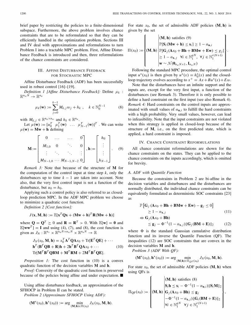
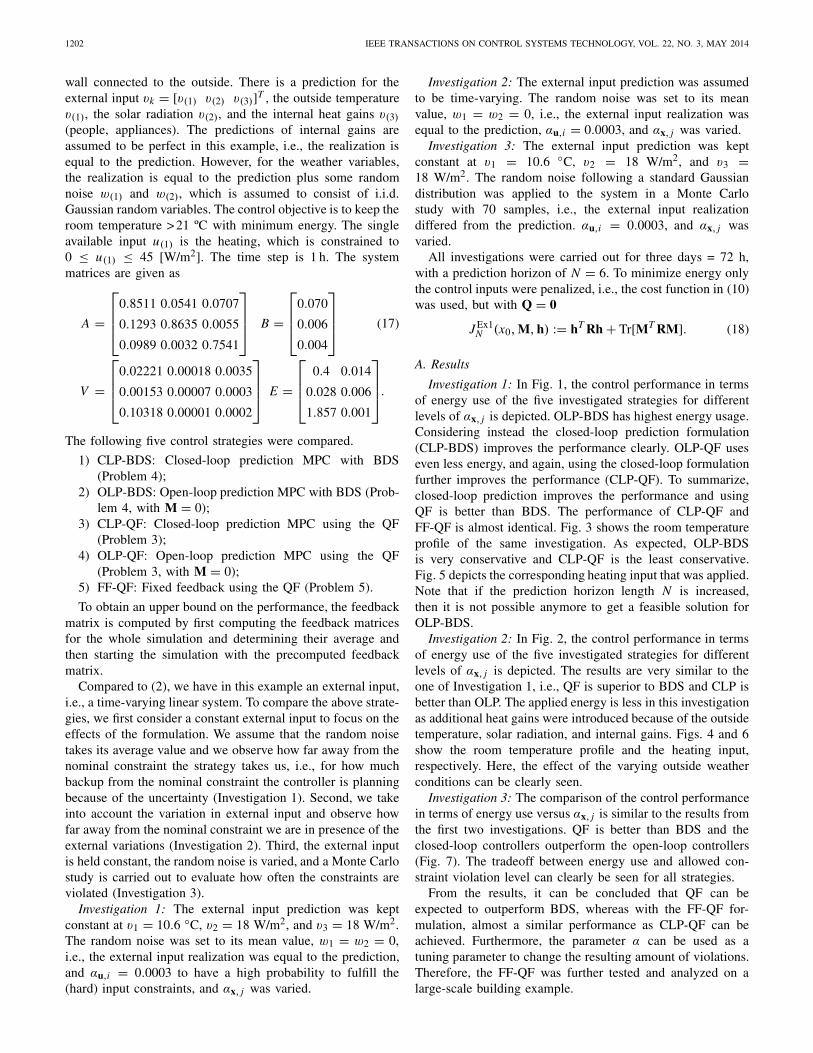
Investigation 1: In Fig. 1, the control performance in termsof energy use of the five investigated strategies for differentlevels of αx, j is depicted. OLP-BDS has highest energy usage.Considering instead the closed-loop prediction formulation(CLP-BDS) improves the performance clearly. OLP-QF useseven less energy, and again, using the closed-loop formulationfurther improves the performance (CLP-QF). To summarize,closed-loop prediction improves the performance and usingQF is better than BDS. The performance of CLP-QF andFF-QF is almost identical. Fig. 3 shows the room temperatureprofile of the same investigation. As expected, OLP-BDSis very conservative and CLP-QF is the least conservative.Fig. 5 depicts the corresponding heating input that was applied.Note that if the prediction horizon length N is increased,then it is not possible anymore to get a feasible solution forOLP-BDS.

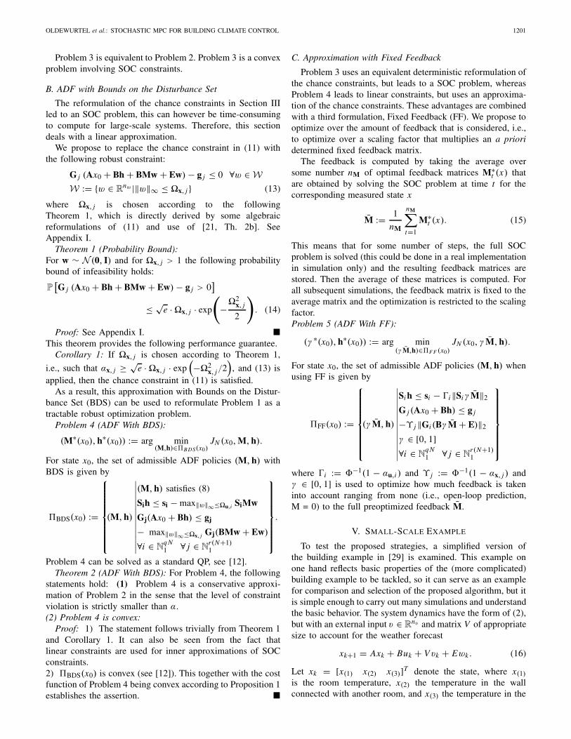
Investigation 2: In Fig. 2, the control performance in termsof energy use of the five investigated strategies for differentlevels of αx, j is depicted. The results are very similar to theone of Investigation 1, i.e., QF is superior to BDS and CLP isbetter than OLP. The applied energy is less in this investigationas additional heat gains were introduced because of the outsidetemperature, solar radiation, and internal gains. Figs. 4 and 6show the room temperature profile and the heating input,respectively. Here, the effect of the varying outside weatherconditions can be clearly seen.

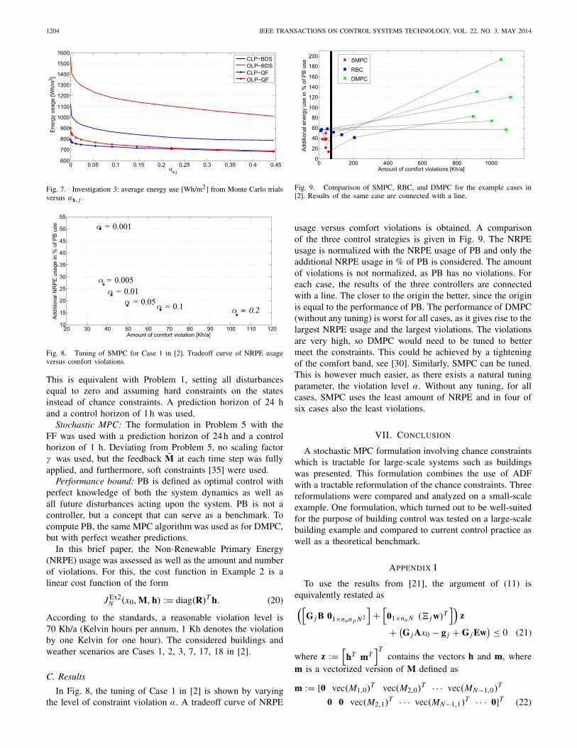
Investigation 3: The comparison of the control performancein terms of energy use versus αx, j is similar to the results fromthe first two investigations. QF is better than BDS and theclosed-loop controllers outperform the open-loop controllers(Fig. 7). The tradeoff between energy use and allowed con-straint violation level can clearly be seen for all strategies.

From the results, it can be concluded that QF can beexpected to outperform BDS, whereas with the FF-QF for-mulation, almost a similar performance as CLP-QF can beachieved. Furthermore, the parameter α can be used as atuning parameter to change the resulting amount of violations.Therefore, the FF-QF was further tested and analyzed on alarge-scale building example.


0 0.05 0.1 0.15 0.2 0.25 0.3 0.35 0.4 0.45400

600

800

1000

1200

1400

1600E

nerg

y us

age

[Wh/

m2 ]

αx,j

CLP−BDSOLP−BDSCLP−QFOLP−QFFF−QF

Fig. 1. Investigation 1: energy use [Wh/m2] versus αx, j .

0 0.05 0.1 0.15 0.2 0.25 0.3 0.35 0.4 0.45400

600

800

1000

1200

1400

1600

Ene

rgy

usag

e [W

h/m

2 ]

αx,j


Fig. 2. Investigation 2: energy use [Wh/m2] versus αx, j .

0 10 20 30 40 50 60 70 8020

22

24

26

28

30

32

Roo

m te

mpe

ratu

re [d

egC

]

Time [h]

CLP−BDSOLP_BDSCLP_QFOLP−QFFF−QF

Fig. 3. Investigation 1: room temperature profile [degC] for αx, j = 0.0003.

VI. EXAMPLE FROM BUILDING CLIMATE CONTROL

The stochastic MPC formulation was primarily motivated bythe use of building control. To determine the energy savingspotential of using stochastic MPC in building control, a large-scale simulation study with different buildings and weatherconditions was carried out in the framework of the projectOptiControl [11]. An excerpt of the results is presented hereto highlight the applicability of the proposed method. Moredetails and analyses can be found in [2], [30], and [31].

A. Modeling

The building dynamics are represented with a bilinearmodel [2], which is augmented by an autoregressive model offirst order driven by Gaussian noise describing the uncertaintyin weather predictions. This uncertainty model is obtainedfrom historical weather data [2] and also used in a Kalmanfilter for filtering the weather predictions. Weather predictionsand measurements are obtained from MeteoSwiss [32]. To deal

0 10 20 30 40 50 60 70 8020

22

24

26

28

30

32

Roo

m te

mpe

ratu

re [d

egC

]

Time [h]


Fig. 4. Investigation 2: room temperature profile [degC] for αx, j = 0.32.

0 10 20 30 40 50 60 70 800

5

10

15

20

25

30

35

40

Hea

ting

inpu

t [W

/m2 ]

Time [h]

CLP−BDSOLP_BDSCLP_QFOLP−QFFF−QF

Fig. 5. Investigation 1: heating [W/m2] for αx, j = 0.0003.

0 10 20 30 40 50 60 70 800

5

10

15

20

25

30

35

40

Hea

ting

inpu

t [W

/m2 ]

Time [h]


Fig. 6. Investigation 2: heating [W/m2] for αx, j = 0.32.

with the bilinear model, we apply a form of sequential linearprogramming, [31], [33], in which we iteratively linearizearound the current solution yielding a time-varying inputmatrix Bu,k . At each time step, an MPC problem for the linearsystem is formulated with the form

xk+1 = Axk + Bu,kuk + V vk + Ewk . (19)

B. Control Strategies and Benchmarks

Three different control strategies were considered in theinvestigation as well as a benchmark. All are listed as follows.

Rule-based control: The standard strategy in current practiceand used by, amongst others, Siemens Building Technologiesis RBC [34]. As the name indicates, RBC determines allcontrol inputs based on a series of rules of the kind if conditionthen action.

Deterministic MPC: This formulation assumes that thedisturbance takes its expected value neglecting the uncertainty.


0 0.05 0.1 0.15 0.2 0.25 0.3 0.35 0.4 0.45600

700

800

900

1000

1100

1200

1300

1400

1500

1600E

nerg

y us

age

[Wh/

m2 ]

αx,j

CLP−BDSOLP−BDSCLP−QFOLP−QF

Fig. 7. Investigation 3: average energy use [Wh/m2] from Monte Carlo trialsversus αx, j .

20 30 40 50 60 70 80 90 100 110 12010

15

20

25

30

35

40

45

50

55

Add

ition

al N

RP

E u

sage

in %

of P

B u

se

Amount of comfort violation [Kh/a]

α = 0.001

α = 0.005α = 0.01

α = 0.05α = 0.1 α = 0.2

Fig. 8. Tuning of SMPC for Case 1 in [2]. Tradeoff curve of NRPE usageversus comfort violations.

This is equivalent with Problem 1, setting all disturbancesequal to zero and assuming hard constraints on the statesinstead of chance constraints. A prediction horizon of 24 hand a control horizon of 1 h was used.

Stochastic MPC: The formulation in Problem 5 with theFF was used with a prediction horizon of 24 h and a controlhorizon of 1 h. Deviating from Problem 5, no scaling factorγ was used, but the feedback M̄ at each time step was fullyapplied, and furthermore, soft constraints [35] were used.

Performance bound: PB is defined as optimal control withperfect knowledge of both the system dynamics as well asall future disturbances acting upon the system. PB is not acontroller, but a concept that can serve as a benchmark. Tocompute PB, the same MPC algorithm was used as for DMPC,but with perfect weather predictions.

In this brief paper, the Non-Renewable Primary Energy(NRPE) usage was assessed as well as the amount and numberof violations. For this, the cost function in Example 2 is alinear cost function of the form

J Ex2N (x0, M, h) := diag(R)T h. (20)

According to the standards, a reasonable violation level is70 Kh/a (Kelvin hours per annum, 1 Kh denotes the violationby one Kelvin for one hour). The considered buildings andweather scenarios are Cases 1, 2, 3, 7, 17, 18 in [2].

C. Results

In Fig. 8, the tuning of Case 1 in [2] is shown by varyingthe level of constraint violation α. A tradeoff curve of NRPE

0 200 400 600 800 10000

20

40

60

80

100

120

140

160

180

200

Add

ition

al e

nerg

y us

e in

% o

f PB

use

Amount of comfort violations [Kh/a]

SMPC

RBCDMPC

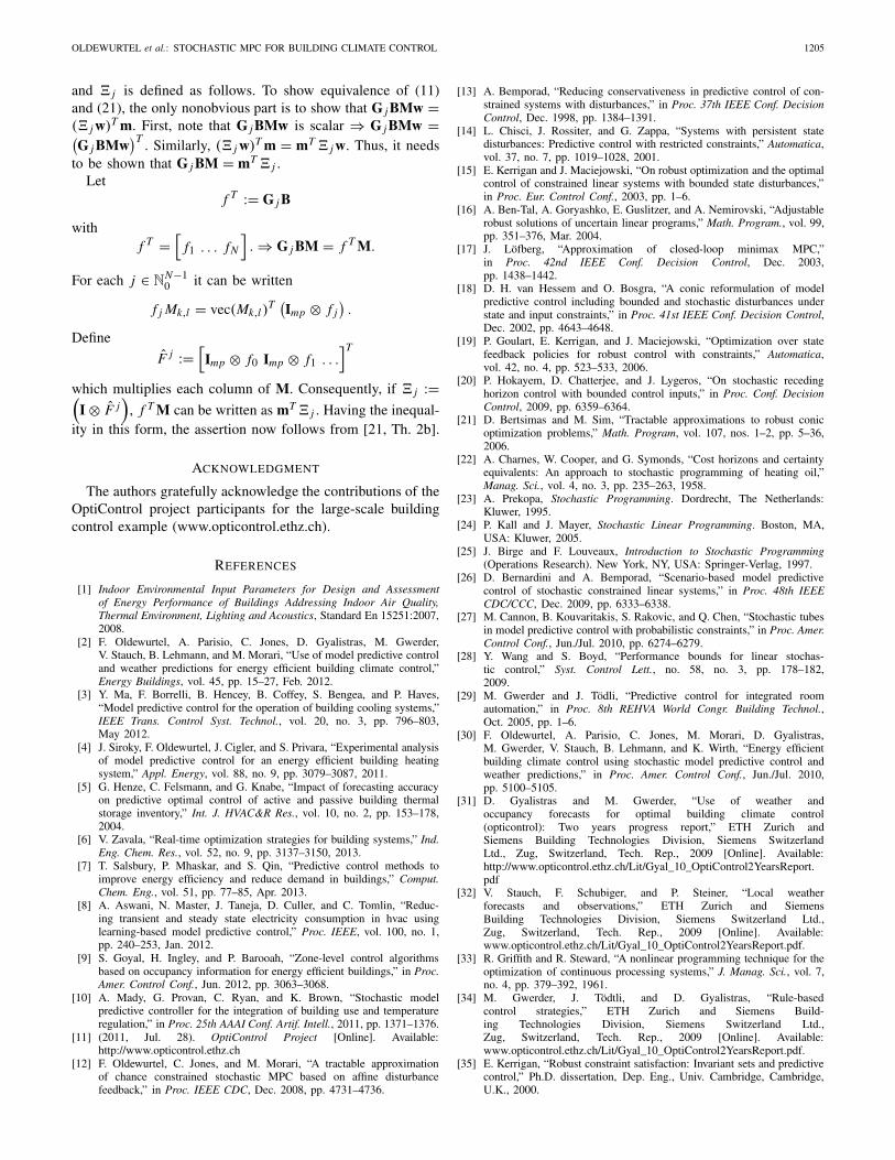
Fig. 9. Comparison of SMPC, RBC, and DMPC for the example cases in[2]. Results of the same case are connected with a line.

usage versus comfort violations is obtained. A comparisonof the three control strategies is given in Fig. 9. The NRPEusage is normalized with the NRPE usage of PB and only theadditional NRPE usage in % of PB is considered. The amountof violations is not normalized, as PB has no violations. Foreach case, the results of the three controllers are connectedwith a line. The closer to the origin the better, since the originis equal to the performance of PB. The performance of DMPC(without any tuning) is worst for all cases, as it gives rise to thelargest NRPE usage and the largest violations. The violationsare very high, so DMPC would need to be tuned to bettermeet the constraints. This could be achieved by a tighteningof the comfort band, see [30]. Similarly, SMPC can be tuned.This is however much easier, as there exists a natural tuningparameter, the violation level α. Without any tuning, for allcases, SMPC uses the least amount of NRPE and in four ofsix cases also the least violations.

VII. CONCLUSION

A stochastic MPC formulation involving chance constraintswhich is tractable for large-scale systems such as buildingswas presented. This formulation combines the use of ADFwith a tractable reformulation of the chance constraints. Threereformulations were compared and analyzed on a small-scaleexample. One formulation, which turned out to be well-suitedfor the purpose of building control was tested on a large-scalebuilding example and compared to current control practice aswell as a theoretical benchmark.

APPENDIX I

To use the results from [21], the argument of (11) isequivalently restated as([

G j B 01×nun p N2

]+

[01×nu N (� j w)T

])z

+ (G j Ax0 − g j + G j Ew

) ≤ 0 (21)

where z :=[hT mT

]Tcontains the vectors h and m, where

m is a vectorized version of M defined as

m := [0 vec(M1,0)T vec(M2,0)

T · · · vec(MN−1,0)T

0 0 vec(M2,1)T · · · vec(MN−1,1)

T · · · 0]T (22)


and � j is defined as follows. To show equivalence of (11)and (21), the only nonobvious part is to show that G j BMw =(� j w)T m. First, note that G j BMw is scalar ⇒ G j BMw =(G j BMw

)T . Similarly, (� j w)T m = mT � j w. Thus, it needsto be shown that G j BM = mT � j .

Letf T := G j B

withf T =

[f1 . . . fN

]. ⇒ G j BM = f T M.

For each j ∈ NN−10 it can be written

f j Mk,l = vec(Mk,l )T (

Imp ⊗ f j).

Define

F̂ j :=[Imp ⊗ f0 Imp ⊗ f1 . . .

]T

which multiplies each column of M. Consequently, if � j :=(I ⊗ F̂ j

), f T M can be written as mT � j . Having the inequal-

ity in this form, the assertion now follows from [21, Th. 2b].

ACKNOWLEDGMENT

The authors gratefully acknowledge the contributions of theOptiControl project participants for the large-scale buildingcontrol example (www.opticontrol.ethz.ch).

REFERENCES

[1] Indoor Environmental Input Parameters for Design and Assessmentof Energy Performance of Buildings Addressing Indoor Air Quality,Thermal Environment, Lighting and Acoustics, Standard En 15251:2007,2008.

[2] F. Oldewurtel, A. Parisio, C. Jones, D. Gyalistras, M. Gwerder,V. Stauch, B. Lehmann, and M. Morari, “Use of model predictive controland weather predictions for energy efficient building climate control,”Energy Buildings, vol. 45, pp. 15–27, Feb. 2012.

[3] Y. Ma, F. Borrelli, B. Hencey, B. Coffey, S. Bengea, and P. Haves,“Model predictive control for the operation of building cooling systems,”IEEE Trans. Control Syst. Technol., vol. 20, no. 3, pp. 796–803,May 2012.

[4] J. Siroky, F. Oldewurtel, J. Cigler, and S. Privara, “Experimental analysisof model predictive control for an energy efficient building heatingsystem,” Appl. Energy, vol. 88, no. 9, pp. 3079–3087, 2011.

[5] G. Henze, C. Felsmann, and G. Knabe, “Impact of forecasting accuracyon predictive optimal control of active and passive building thermalstorage inventory,” Int. J. HVAC&R Res., vol. 10, no. 2, pp. 153–178,2004.

[6] V. Zavala, “Real-time optimization strategies for building systems,” Ind.Eng. Chem. Res., vol. 52, no. 9, pp. 3137–3150, 2013.

[7] T. Salsbury, P. Mhaskar, and S. Qin, “Predictive control methods toimprove energy efficiency and reduce demand in buildings,” Comput.Chem. Eng., vol. 51, pp. 77–85, Apr. 2013.

[8] A. Aswani, N. Master, J. Taneja, D. Culler, and C. Tomlin, “Reduc-ing transient and steady state electricity consumption in hvac usinglearning-based model predictive control,” Proc. IEEE, vol. 100, no. 1,pp. 240–253, Jan. 2012.

[9] S. Goyal, H. Ingley, and P. Barooah, “Zone-level control algorithmsbased on occupancy information for energy efficient buildings,” in Proc.Amer. Control Conf., Jun. 2012, pp. 3063–3068.

[10] A. Mady, G. Provan, C. Ryan, and K. Brown, “Stochastic modelpredictive controller for the integration of building use and temperatureregulation,” in Proc. 25th AAAI Conf. Artif. Intell., 2011, pp. 1371–1376.

[11] (2011, Jul. 28). OptiControl Project [Online]. Available:http://www.opticontrol.ethz.ch

[12] F. Oldewurtel, C. Jones, and M. Morari, “A tractable approximationof chance constrained stochastic MPC based on affine disturbancefeedback,” in Proc. IEEE CDC, Dec. 2008, pp. 4731–4736.

[13] A. Bemporad, “Reducing conservativeness in predictive control of con-strained systems with disturbances,” in Proc. 37th IEEE Conf. DecisionControl, Dec. 1998, pp. 1384–1391.

[14] L. Chisci, J. Rossiter, and G. Zappa, “Systems with persistent statedisturbances: Predictive control with restricted constraints,” Automatica,vol. 37, no. 7, pp. 1019–1028, 2001.

[15] E. Kerrigan and J. Maciejowski, “On robust optimization and the optimalcontrol of constrained linear systems with bounded state disturbances,”in Proc. Eur. Control Conf., 2003, pp. 1–6.

[16] A. Ben-Tal, A. Goryashko, E. Guslitzer, and A. Nemirovski, “Adjustablerobust solutions of uncertain linear programs,” Math. Program., vol. 99,pp. 351–376, Mar. 2004.

[17] J. Löfberg, “Approximation of closed-loop minimax MPC,”in Proc. 42nd IEEE Conf. Decision Control, Dec. 2003,pp. 1438–1442.

[18] D. H. van Hessem and O. Bosgra, “A conic reformulation of modelpredictive control including bounded and stochastic disturbances understate and input constraints,” in Proc. 41st IEEE Conf. Decision Control,Dec. 2002, pp. 4643–4648.

[19] P. Goulart, E. Kerrigan, and J. Maciejowski, “Optimization over statefeedback policies for robust control with constraints,” Automatica,vol. 42, no. 4, pp. 523–533, 2006.

[20] P. Hokayem, D. Chatterjee, and J. Lygeros, “On stochastic recedinghorizon control with bounded control inputs,” in Proc. Conf. DecisionControl, 2009, pp. 6359–6364.

[21] D. Bertsimas and M. Sim, “Tractable approximations to robust conicoptimization problems,” Math. Program, vol. 107, nos. 1–2, pp. 5–36,2006.

[22] A. Charnes, W. Cooper, and G. Symonds, “Cost horizons and certaintyequivalents: An approach to stochastic programming of heating oil,”Manag. Sci., vol. 4, no. 3, pp. 235–263, 1958.

[23] A. Prekopa, Stochastic Programming. Dordrecht, The Netherlands:Kluwer, 1995.

[24] P. Kall and J. Mayer, Stochastic Linear Programming. Boston, MA,USA: Kluwer, 2005.

[25] J. Birge and F. Louveaux, Introduction to Stochastic Programming(Operations Research). New York, NY, USA: Springer-Verlag, 1997.

[26] D. Bernardini and A. Bemporad, “Scenario-based model predictivecontrol of stochastic constrained linear systems,” in Proc. 48th IEEECDC/CCC, Dec. 2009, pp. 6333–6338.

[27] M. Cannon, B. Kouvaritakis, S. Rakovic, and Q. Chen, “Stochastic tubesin model predictive control with probabilistic constraints,” in Proc. Amer.Control Conf., Jun./Jul. 2010, pp. 6274–6279.

[28] Y. Wang and S. Boyd, “Performance bounds for linear stochas-tic control,” Syst. Control Lett., no. 58, no. 3, pp. 178–182,2009.

[29] M. Gwerder and J. Tödli, “Predictive control for integrated roomautomation,” in Proc. 8th REHVA World Congr. Building Technol.,Oct. 2005, pp. 1–6.

[30] F. Oldewurtel, A. Parisio, C. Jones, M. Morari, D. Gyalistras,M. Gwerder, V. Stauch, B. Lehmann, and K. Wirth, “Energy efficientbuilding climate control using stochastic model predictive control andweather predictions,” in Proc. Amer. Control Conf., Jun./Jul. 2010,pp. 5100–5105.

[31] D. Gyalistras and M. Gwerder, “Use of weather andoccupancy forecasts for optimal building climate control(opticontrol): Two years progress report,” ETH Zurich andSiemens Building Technologies Division, Siemens SwitzerlandLtd., Zug, Switzerland, Tech. Rep., 2009 [Online]. Available:http://www.opticontrol.ethz.ch/Lit/Gyal_10_OptiControl2YearsReport.pdf

[32] V. Stauch, F. Schubiger, and P. Steiner, “Local weatherforecasts and observations,” ETH Zurich and SiemensBuilding Technologies Division, Siemens Switzerland Ltd.,Zug, Switzerland, Tech. Rep., 2009 [Online]. Available:www.opticontrol.ethz.ch/Lit/Gyal_10_OptiControl2YearsReport.pdf.

[33] R. Griffith and R. Steward, “A nonlinear programming technique for theoptimization of continuous processing systems,” J. Manag. Sci., vol. 7,no. 4, pp. 379–392, 1961.

[34] M. Gwerder, J. Tödtli, and D. Gyalistras, “Rule-basedcontrol strategies,” ETH Zurich and Siemens Build-ing Technologies Division, Siemens Switzerland Ltd.,Zug, Switzerland, Tech. Rep., 2009 [Online]. Available:www.opticontrol.ethz.ch/Lit/Gyal_10_OptiControl2YearsReport.pdf.

[35] E. Kerrigan, “Robust constraint satisfaction: Invariant sets and predictivecontrol,” Ph.D. dissertation, Dep. Eng., Univ. Cambridge, Cambridge,U.K., 2000.

Documents

Stochastic Model Predictive Control for Building Climate Control