Stochastic Network Utility Maximization

Stochastic Network Utility Maximization

Igor Kadota

Cambridge, December 07, 2018

6.263/16.37 - Data Communication Networks

Outline• Multi-commodity flow problem• Recap from previous lectures

• Network of Queues• Capacity Region and Stationary Randomized Policy

• Overloaded system• Problem Statement• Utility Function• Drift-Plus Penalty Algorithm (Admission + Routing + Scheduling)• Performance Analysis and Optimality Results

*slides adapted from Chih-Ping Li’s lecture, with additional material from “Resource Allocation and Cross-Layer Control in Wireless Networks” by L. Georgiadis, M. J. Neely and L. Tassiulas and from M. J. Neely’s PhD thesis.

Multi-Commodity Flow Problem

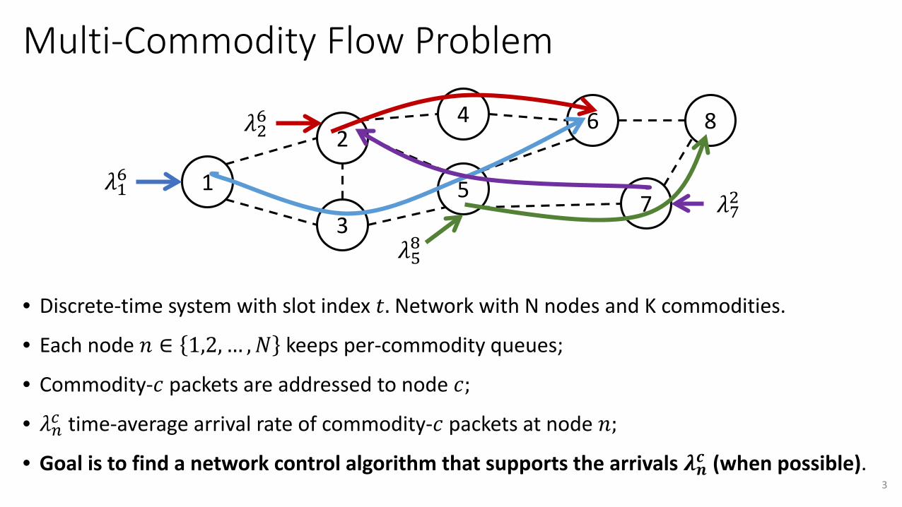
• Discrete-time system with slot index 𝑡𝑡. Network with N nodes and K commodities.

• Each node 𝑛𝑛 ∈ 1,2, … ,𝑁𝑁 keeps per-commodity queues;

• Commodity-𝑐𝑐 packets are addressed to node 𝑐𝑐;

• 𝜆𝜆𝑛𝑛𝑐𝑐 time-average arrival rate of commodity-𝑐𝑐 packets at node 𝑛𝑛;

• Goal is to find a network control algorithm that supports the arrivals 𝝀𝝀𝒏𝒏𝒄𝒄 (when possible).3

1

2

3

4

5 7

6 8

𝜆𝜆16

𝜆𝜆58𝜆𝜆72

𝜆𝜆26

Network of Queues• Let 𝑄𝑄𝑛𝑛𝑐𝑐(𝑡𝑡) be the number of commodity-𝑐𝑐 packets enqueued at node 𝑛𝑛 at the beginning of

time-slot 𝑡𝑡. Then, according to Lindley recursion:

where:

• 𝐴𝐴𝑛𝑛𝑐𝑐 𝑡𝑡 ≥ 0 is the number of exogenous packet arrivals at the end of slot 𝑡𝑡;

• 𝜇𝜇𝑛𝑛,𝑗𝑗𝑐𝑐 (𝑡𝑡) ≥ 0 is the offered transmission opportunity to comm.-𝑐𝑐 over (𝑛𝑛, 𝑗𝑗) during slot 𝑡𝑡;

• 𝜇𝜇𝑛𝑛,𝑗𝑗 𝑡𝑡 = ∑𝑐𝑐=1𝐾𝐾 𝜇𝜇𝑛𝑛,𝑗𝑗𝑐𝑐 (𝑡𝑡) is the total transmission opportunity over (𝑛𝑛, 𝑗𝑗) during slot 𝑡𝑡;

• 0 ≤ 𝑓𝑓𝑛𝑛,𝑗𝑗𝑐𝑐 𝑡𝑡 ≤ 𝜇𝜇𝑛𝑛,𝑗𝑗

𝑐𝑐 (𝑡𝑡) is the # of packet transmissions of comm.-c over (𝑛𝑛, 𝑗𝑗) during slot 𝑡𝑡;

• 𝒞𝒞𝑛𝑛,𝑗𝑗 is the capacity constraint of link 𝑛𝑛, 𝑗𝑗 .

4

𝑄𝑄𝑛𝑛𝑐𝑐 𝑡𝑡 + 1 ≤ max 𝑄𝑄𝑛𝑛𝑐𝑐 𝑡𝑡 −�𝑗𝑗=1

𝑁𝑁𝜇𝜇𝑛𝑛,𝑗𝑗𝑐𝑐 𝑡𝑡 ; 0 + �

𝑖𝑖=1

𝑁𝑁𝜇𝜇𝑖𝑖,𝑛𝑛𝑐𝑐 𝑡𝑡 + 𝐴𝐴𝑛𝑛𝑐𝑐 𝑡𝑡



where:

• 𝐴𝐴𝑛𝑛𝑐𝑐 𝑡𝑡 ≥ 0 is the number of exogenous packet arrivals at the end of slot 𝑡𝑡;

• 𝜇𝜇𝑛𝑛,𝑗𝑗𝑐𝑐 (𝑡𝑡) ≥ 0 is the offered transmission opportunity to comm.-𝑐𝑐 over (𝑛𝑛, 𝑗𝑗) during slot 𝑡𝑡;

• 𝜇𝜇𝑛𝑛,𝑗𝑗 𝑡𝑡 = ∑𝑐𝑐=1𝐾𝐾 𝜇𝜇𝑛𝑛,𝑗𝑗𝑐𝑐 (𝑡𝑡) is the total transmission opportunity over (𝑛𝑛, 𝑗𝑗) during slot 𝑡𝑡;

• 0 ≤ 𝑓𝑓𝑛𝑛,𝑗𝑗𝑐𝑐 𝑡𝑡 ≤ 𝜇𝜇𝑛𝑛,𝑗𝑗

𝑐𝑐 (𝑡𝑡) is the # of packet transmissions of comm.-c over (𝑛𝑛, 𝑗𝑗) during slot 𝑡𝑡;

• 𝒞𝒞𝑛𝑛,𝑗𝑗 is the capacity constraint of link 𝑛𝑛, 𝑗𝑗 .

5

𝑄𝑄𝑛𝑛𝑐𝑐 𝑡𝑡 + 1 = 𝑄𝑄𝑛𝑛𝑐𝑐 𝑡𝑡 −�𝑗𝑗=1

𝑁𝑁𝑓𝑓𝑛𝑛,𝑗𝑗𝑐𝑐 𝑡𝑡 + �

𝑖𝑖=1

𝑁𝑁𝑓𝑓𝑖𝑖,𝑛𝑛𝑐𝑐 𝑡𝑡 + 𝐴𝐴𝑛𝑛𝑐𝑐 𝑡𝑡



Constraints:

6



𝑖𝑖=1


jn

1

N

𝒇𝒇𝒏𝒏,𝟏𝟏𝒄𝒄 𝒕𝒕

𝒇𝒇𝒏𝒏,𝒋𝒋𝒄𝒄 𝒕𝒕

𝒇𝒇𝒏𝒏,𝑵𝑵𝒄𝒄 𝒕𝒕

i

𝑸𝑸𝒏𝒏𝒄𝒄 𝒕𝒕

jn𝒇𝒇𝒏𝒏,𝒋𝒋𝟏𝟏 𝒕𝒕𝒇𝒇𝒏𝒏,𝒋𝒋𝒄𝒄 𝒕𝒕

𝒇𝒇𝒏𝒏,𝒋𝒋𝑲𝑲 𝒕𝒕

i𝝁𝝁𝒏𝒏,𝒋𝒋 𝒕𝒕

∑𝑗𝑗=1𝑁𝑁 𝑓𝑓𝑛𝑛,𝑗𝑗𝑐𝑐 𝑡𝑡 ≤ 𝑄𝑄𝑛𝑛𝑐𝑐 𝑡𝑡 ,∀𝑛𝑛, 𝑐𝑐, 𝑡𝑡 ∑𝑐𝑐=1𝐾𝐾 𝑓𝑓𝑛𝑛,𝑗𝑗

𝑐𝑐 𝑡𝑡 ≤ 𝜇𝜇𝑛𝑛,𝑗𝑗 𝑡𝑡 ≤ 𝒞𝒞𝑛𝑛,𝑗𝑗 ,∀𝑛𝑛, 𝑗𝑗, 𝑡𝑡

𝓒𝓒𝒏𝒏,𝒋𝒋



Assumptions:

7



𝑖𝑖=1


lim𝑡𝑡→∞

1𝑡𝑡�

𝜏𝜏=0

𝑡𝑡−1𝐴𝐴𝑛𝑛𝑐𝑐 𝜏𝜏 = 𝜆𝜆𝑛𝑛𝑐𝑐 w. p. 1

lim𝑡𝑡→∞

1𝑡𝑡�

𝜏𝜏=0

𝑡𝑡−1𝑓𝑓𝑛𝑛,𝑗𝑗𝑐𝑐 𝜏𝜏 = ̅𝑓𝑓𝑛𝑛,𝑗𝑗

𝑐𝑐 w. p. 1i jn

𝑓𝑓𝑖𝑖,𝑛𝑛𝑐𝑐 𝑡𝑡 𝑓𝑓𝑛𝑛,𝑗𝑗𝑐𝑐 𝑡𝑡

𝑨𝑨𝒏𝒏𝒄𝒄 𝒕𝒕𝜇𝜇𝑖𝑖,𝑛𝑛 𝑡𝑡 𝜇𝜇𝑛𝑛,𝑗𝑗 𝑡𝑡

lim𝑡𝑡→∞

1𝑡𝑡�

𝜏𝜏=0

𝑡𝑡−1𝜇𝜇𝑛𝑛,𝑗𝑗𝑐𝑐 𝜏𝜏 = �̅�𝜇𝑛𝑛,𝑗𝑗

𝑐𝑐 w. p. 1

Network of Queues – Stability is the objective

• Rate stability:

• Queue 𝑄𝑄𝑛𝑛𝑐𝑐(𝑡𝑡) is rate stable if and only if

• If Arrival > Departure, then:

• Strong stability: [bounded time-average queue backlog]

• If 𝑄𝑄𝑛𝑛𝑐𝑐(𝑡𝑡) is strongly stable and there exists 𝐶𝐶 > 0 such that

𝑎𝑎𝑎𝑎𝑎𝑎 𝑡𝑡 − 𝑑𝑑𝑑𝑑𝑑𝑑_𝑜𝑜𝑑𝑑𝑑𝑑(𝑡𝑡) ≤ 𝐶𝐶 w. p. 1,∀𝑡𝑡 or 𝑑𝑑𝑑𝑑𝑑𝑑_𝑜𝑜𝑑𝑑𝑑𝑑 𝑡𝑡 − 𝑎𝑎𝑎𝑎𝑎𝑎 𝑡𝑡 ≤ 𝐶𝐶 w. p. 1,∀𝑡𝑡

Then 𝑄𝑄𝑛𝑛𝑐𝑐(𝑡𝑡) is also Rate Stable.8

lim𝑡𝑡→∞

𝑄𝑄𝑛𝑛𝑐𝑐(𝑡𝑡)𝑡𝑡

= 0 w. p. 1

lim𝑡𝑡→∞

𝑄𝑄𝑛𝑛𝑐𝑐(𝑡𝑡)𝑡𝑡

= �𝑖𝑖=1

𝑁𝑁̅𝑓𝑓𝑖𝑖,𝑛𝑛𝑐𝑐 + 𝜆𝜆𝑛𝑛𝑐𝑐 −�

𝑗𝑗=1

𝑁𝑁̅𝑓𝑓𝑛𝑛,𝑗𝑗𝑐𝑐 w. p. 1

lim𝑡𝑡→∞

1𝑡𝑡�𝜏𝜏=0

𝑡𝑡−1

𝔼𝔼 𝑄𝑄𝑛𝑛𝑐𝑐(𝜏𝜏) < ∞

�𝑖𝑖=1

𝑁𝑁̅𝑓𝑓𝑖𝑖,𝑛𝑛𝑐𝑐 + 𝜆𝜆𝑛𝑛𝑐𝑐 = �

𝑗𝑗=1

𝑁𝑁̅𝑓𝑓𝑛𝑛,𝑗𝑗𝑐𝑐 ≤�

𝑗𝑗=1

𝑁𝑁�̅�𝜇𝑛𝑛,𝑗𝑗𝑐𝑐

Arrival Rate = Departure ≤ Dep. Opport.

Network of Queues – Action and Outcome• Network State: 𝑠𝑠 𝑡𝑡 ∈ 𝒮𝒮 ← channels, topology, packet arrivals,… [uncontrollable]

• Assumption: s(t) evolves according to an irreducible MC with finite states such that :

• Action: 𝐼𝐼 𝑡𝑡 ∈ ℐ𝑠𝑠 𝑡𝑡 ← controls 𝜇𝜇𝑖𝑖,𝑗𝑗(𝑡𝑡) and 𝑓𝑓𝑖𝑖,𝑗𝑗𝑐𝑐 (𝑡𝑡) using knowledge of the network state and (possibly) other information such as current queue backlog.𝐼𝐼 𝑡𝑡 satisfies constraints from the state space ℐ𝑠𝑠 𝑡𝑡 .

• Outcome: the result of any given state action pair (𝑠𝑠 𝑡𝑡 , 𝐼𝐼(𝑡𝑡)) are: 1) 𝐴𝐴𝑛𝑛𝑐𝑐 𝑡𝑡 for every node 𝑛𝑛 and; 2) 𝜇𝜇𝑖𝑖,𝑗𝑗(𝑡𝑡) and 𝑓𝑓𝑖𝑖,𝑗𝑗𝑐𝑐 (𝑡𝑡) for every link (𝑖𝑖, 𝑗𝑗) and commodity 𝑐𝑐.

• Define the (total) link transmission rate matrix as 𝑼𝑼 𝑠𝑠 𝑡𝑡 , 𝐼𝐼 𝑡𝑡 = 𝜇𝜇𝑖𝑖,𝑗𝑗 𝑡𝑡 𝑖𝑖,𝑗𝑗.

9

lim𝑡𝑡→∞

1𝑡𝑡�

𝜏𝜏=0

𝑡𝑡−1𝔗𝔗𝑛𝑛𝑑𝑑𝑖𝑖𝑐𝑐𝑎𝑎𝑡𝑡𝑜𝑜𝑎𝑎 𝑠𝑠 𝜏𝜏 =𝑠𝑠 = 𝜋𝜋𝑠𝑠 w. p. 1. ; ∀𝑠𝑠 ∈ 𝒮𝒮

Capacity Region – Definition Definition: Capacity Region Λ is the closure of the set of all arrival rate matrices 𝜆𝜆𝑛𝑛𝑐𝑐 𝑛𝑛,𝑐𝑐 that can be stabilized by some (possibly unknown) network control algorithm.

Example: wireline network with capacity 𝒞𝒞𝑛𝑛,𝑗𝑗. State is 𝑠𝑠 𝑡𝑡 = all channels are ON,∀𝑡𝑡.

10

1 4

2𝐴𝐴14 𝑡𝑡

3

𝒞𝒞1,2

𝒞𝒞1,3

𝒞𝒞2,4

𝒞𝒞3,4

The capacity region Λ is given by the set of all 𝜆𝜆14, 𝜆𝜆34for which there exists flow variables ̅𝑓𝑓𝑛𝑛,𝑗𝑗

𝑐𝑐 satisfying:

Capacity: ∑𝑐𝑐=1𝐾𝐾 ̅𝑓𝑓𝑖𝑖,𝑗𝑗𝑐𝑐 ≤ 𝒞𝒞𝑖𝑖,𝑗𝑗 ,∀𝑖𝑖, 𝑗𝑗;

Conservation: 𝜆𝜆𝑛𝑛𝑐𝑐 = ∑𝑗𝑗=1𝑁𝑁 ̅𝑓𝑓𝑛𝑛,𝑗𝑗𝑐𝑐 − ∑𝑖𝑖=1𝑁𝑁 ̅𝑓𝑓𝑖𝑖,𝑛𝑛𝑐𝑐 ,∀𝑛𝑛, 𝑐𝑐;

𝐴𝐴34 𝑡𝑡Notice similarity between flow conservation and the necessary and sufficient conditions for rate stability.

Capacity Region – Definition Definition: Capacity Region Λ is the closure of the set of all arrival rate matrices 𝜆𝜆𝑛𝑛𝑐𝑐 𝑛𝑛,𝑐𝑐 that can be stabilized by some (possibly unknown) network control algorithm.

Supported transmission rate matrices: 𝒞𝒞𝒞𝒞 Γ

• Consider a fixed state 𝑠𝑠 ∈ 𝒮𝒮 and define the set 𝐴𝐴𝑠𝑠 of all possible transmission rate matrices:

𝐴𝐴𝑠𝑠 ≔ 𝑼𝑼 𝑠𝑠, 𝐼𝐼 = 𝜇𝜇𝑖𝑖,𝑗𝑗 𝑡𝑡 𝑖𝑖,𝑗𝑗𝐼𝐼 ∈ ℐ𝑠𝑠

• Consider the Stationary Randomized policy which selects 𝐼𝐼 𝑡𝑡 = 𝐼𝐼 w.p. 𝑑𝑑𝑠𝑠 𝐼𝐼 ∈ (0,1].

• This stationary policy attains 𝔼𝔼 𝜇𝜇𝑖𝑖,𝑗𝑗 𝑡𝑡 𝑖𝑖,𝑗𝑗𝑠𝑠 𝑡𝑡 = 𝑠𝑠 ∈ 𝐶𝐶𝑜𝑜𝑛𝑛𝐶𝐶𝐶𝐶𝐶𝐶𝒞𝒞𝒞𝒞 𝐴𝐴𝑠𝑠 .

• By appropriately selecting 𝑑𝑑𝑠𝑠(𝐼𝐼), any point in 𝐶𝐶𝑜𝑜𝑛𝑛𝐶𝐶𝐶𝐶𝐶𝐶𝒞𝒞𝒞𝒞 𝐴𝐴𝑠𝑠 can be achieved.

• The long-term link transmission rate matrix achieved by the class of Stationary Randomized policies is defined as Γ ≔ ∑𝑠𝑠∈𝒮𝒮 𝜋𝜋𝑠𝑠𝐶𝐶𝑜𝑜𝑛𝑛𝐶𝐶𝐶𝐶𝐶𝐶𝒞𝒞𝒞𝒞 𝐴𝐴𝑠𝑠 and its closure is denoted 𝒞𝒞𝒞𝒞 Γ .

11

Capacity Region – DefinitionDefinition: Capacity Region Λ is the closure of the set of all arrival rate matrices 𝜆𝜆𝑛𝑛𝑐𝑐 𝑛𝑛,𝑐𝑐 that can be stabilized by some (possibly unknown) network control algorithm.

Illustration:

*figure adapted from the book “Resource Allocation and Cross-Layer Control in Wireless Networks” 12

𝑨𝑨𝒔𝒔𝟐𝟐 = 𝑼𝑼 𝑠𝑠2, 𝐼𝐼 𝐼𝐼 ∈ ℐ𝒔𝒔𝟐𝟐

𝑨𝑨𝒔𝒔𝟏𝟏 = 𝑼𝑼 𝑠𝑠1, 𝐼𝐼 𝐼𝐼 ∈ ℐ𝒔𝒔𝟏𝟏

𝐶𝐶𝑜𝑜𝑛𝑛𝐶𝐶𝐶𝐶𝐶𝐶𝒞𝒞𝒞𝒞 𝑨𝑨𝒔𝒔𝟏𝟏

𝔼𝔼 𝜇𝜇2 𝜞𝜞 = �𝑠𝑠∈𝒮𝒮

𝜋𝜋𝑠𝑠𝐶𝐶𝑜𝑜𝑛𝑛𝐶𝐶𝐶𝐶𝐶𝐶𝒞𝒞𝒞𝒞 𝐴𝐴𝑠𝑠

𝔼𝔼 𝜇𝜇1

𝔼𝔼 𝜇𝜇2

𝔼𝔼 𝜇𝜇1

Capacity Region – TheoremDefinition: Capacity Region Λ is the closure of the set of all arrival rate matrices 𝜆𝜆𝑛𝑛𝑐𝑐 𝑛𝑛,𝑐𝑐 that can be stabilized by some (possibly unknown) network control algorithm.

Theorem: the capacity region Λ is given by the set of arrival rate matrices 𝜆𝜆𝑛𝑛𝑐𝑐 𝑛𝑛,𝑐𝑐 for which there exists a transmission rate matrix 𝔼𝔼 𝜇𝜇𝑖𝑖,𝑗𝑗 𝑡𝑡 𝑖𝑖,𝑗𝑗

= �̅�𝜇𝑖𝑖,𝑗𝑗 𝑖𝑖,𝑗𝑗∈ 𝒞𝒞𝒞𝒞 Γ together with multi-

commodity flow variables ̅𝑓𝑓𝑖𝑖,𝑗𝑗𝑐𝑐 that satisfy the following routing feasibility constraints:

• Flow capacity: ∑𝑐𝑐=1𝐾𝐾 ̅𝑓𝑓𝑖𝑖,𝑗𝑗𝑐𝑐 ≤ �̅�𝜇𝑖𝑖,𝑗𝑗 ≤ 𝒞𝒞𝑖𝑖,𝑗𝑗 ,∀𝑖𝑖, 𝑗𝑗;

• Flow conservation: 𝜆𝜆𝑛𝑛𝑐𝑐 = ∑𝑗𝑗=1𝑁𝑁 ̅𝑓𝑓𝑛𝑛,𝑗𝑗𝑐𝑐 − ∑𝑖𝑖=1𝑁𝑁 ̅𝑓𝑓𝑖𝑖,𝑛𝑛𝑐𝑐 ,∀𝑛𝑛, 𝑐𝑐;

• Flow are efficient: ̅𝑓𝑓𝑖𝑖,𝑖𝑖𝑐𝑐 = 0, ̅𝑓𝑓𝑐𝑐,𝑖𝑖𝑐𝑐 = 0; [no flow from a node to itself or from the destination]

• Flows are non-negative: ̅𝑓𝑓𝑖𝑖,𝑗𝑗𝑐𝑐 ≥ 0,∀𝑖𝑖, 𝑗𝑗, 𝑐𝑐;

• Routing constraints: ̅𝑓𝑓𝑖𝑖,𝑗𝑗𝑐𝑐 = 0,∀ 𝑖𝑖, 𝑗𝑗, 𝑐𝑐 for which flow is not allowed. 13

Capacity Region – Example On/Off downlink• i.i.d. Bernoulli channel state with ℙ 𝑠𝑠1 𝑡𝑡 = 𝑂𝑂𝑁𝑁 = 𝑑𝑑1 and ℙ 𝑠𝑠2 𝑡𝑡 = 𝑂𝑂𝑁𝑁 = 𝑑𝑑2• Every time-slot t, the controller observes the channels 𝑠𝑠𝑛𝑛 𝑡𝑡 and serves at most one packet

from one of the queues: 𝜇𝜇𝑛𝑛 𝑡𝑡 ∈ {0,1} such that 𝜇𝜇1 𝑡𝑡 + 𝜇𝜇2 𝑡𝑡 ≤ 1,∀𝑡𝑡.

• Long-term link transmission rate matrix:

14

State Probability Transmission Rates(OFF,OFF) (1-p1)(1-p2) (0,0)(ON,OFF) p1(1-p2) (0,0), (1,0)(OFF,ON) (1-p1)p2 (0,0), (0,1)(ON,ON) p1p2 (0,0), (1,0), (0,1)

𝑑𝑑1

𝑑𝑑2

𝜞𝜞 = 1 − 𝑑𝑑1 1 − 𝑑𝑑2 𝟎𝟎,𝟎𝟎 + 𝑑𝑑1 1 − 𝑑𝑑2 𝑪𝑪𝑪𝑪𝒏𝒏𝑪𝑪𝑪𝑪𝑪𝑪𝑪𝑪𝑪𝑪 𝟎𝟎,𝟎𝟎 , 𝟏𝟏,𝟎𝟎 +

+ 1 − 𝑑𝑑1 𝑑𝑑2𝑪𝑪𝑪𝑪𝒏𝒏𝑪𝑪𝑪𝑪𝑪𝑪𝑪𝑪𝑪𝑪 𝟎𝟎,𝟎𝟎 , 𝟎𝟎,𝟏𝟏 + 𝑑𝑑1𝑑𝑑2𝑪𝑪𝑪𝑪𝒏𝒏𝑪𝑪𝑪𝑪𝑪𝑪𝑪𝑪𝑪𝑪 𝟎𝟎,𝟎𝟎 , 𝟎𝟎,𝟏𝟏 , 𝟏𝟏,𝟎𝟎




15

𝜞𝜞 = 1 − 𝑑𝑑1 1 − 𝑑𝑑2 𝟎𝟎,𝟎𝟎 + 𝑑𝑑1 1 − 𝑑𝑑2 𝒒𝒒𝟏𝟏,𝟎𝟎 + 1 − 𝑑𝑑1 𝑑𝑑2 𝟎𝟎,𝒒𝒒𝟐𝟐 + 𝑑𝑑1𝑑𝑑2 𝟏𝟏 − 𝒒𝒒𝟑𝟑,𝒒𝒒𝟑𝟑

𝜞𝜞 = 𝑑𝑑1 1 − 𝑑𝑑2 𝒒𝒒𝟏𝟏 + 𝑑𝑑1𝑑𝑑2 𝟏𝟏 − 𝒒𝒒𝟑𝟑 , 1 − 𝑑𝑑1 𝑑𝑑2𝒒𝒒𝟐𝟐 + 𝑑𝑑1𝑑𝑑2𝒒𝒒𝟑𝟑 , for 𝑞𝑞 ∈ 0,1

𝜞𝜞 = 1 − 𝑑𝑑1 1 − 𝑑𝑑2 𝟎𝟎,𝟎𝟎 + 𝑑𝑑1 1 − 𝑑𝑑2 𝑪𝑪𝑪𝑪𝒏𝒏𝑪𝑪𝑪𝑪𝑪𝑪𝑪𝑪𝑪𝑪 𝟎𝟎,𝟎𝟎 , 𝟏𝟏,𝟎𝟎 +

+ 1 − 𝑑𝑑1 𝑑𝑑2𝑪𝑪𝑪𝑪𝒏𝒏𝑪𝑪𝑪𝑪𝑪𝑪𝑪𝑪𝑪𝑪 𝟎𝟎,𝟎𝟎 , 𝟎𝟎,𝟏𝟏 + 𝑑𝑑1𝑑𝑑2𝑪𝑪𝑪𝑪𝒏𝒏𝑪𝑪𝑪𝑪𝑪𝑪𝑪𝑪𝑪𝑪 𝟎𝟎,𝟎𝟎 , 𝟎𝟎,𝟏𝟏 , 𝟏𝟏,𝟎𝟎




16

𝑑𝑑2

𝑑𝑑1

𝔼𝔼 𝜇𝜇2

𝔼𝔼 𝜇𝜇1

𝜞𝜞 = 𝑑𝑑1 1 − 𝑑𝑑2 𝒒𝒒𝟏𝟏 + 𝑑𝑑1𝑑𝑑2 𝟏𝟏 − 𝒒𝒒𝟑𝟑 , 1 − 𝑑𝑑1 𝑑𝑑2𝒒𝒒𝟐𝟐 + 𝑑𝑑1𝑑𝑑2𝒒𝒒𝟑𝟑

𝜞𝜞

𝑑𝑑1

𝑑𝑑2

Capacity Region – Example On/Off downlink• i.i.d. Bernoulli packet arrivals with ℙ 𝑨𝑨𝟏𝟏 𝒕𝒕 = 𝟏𝟏 = 𝝀𝝀𝟏𝟏 and ℙ 𝑨𝑨𝟐𝟐 𝒕𝒕 = 𝟏𝟏 = 𝝀𝝀𝟐𝟐.• i.i.d. Bernoulli channel state with ℙ 𝑠𝑠1 𝑡𝑡 = 𝑂𝑂𝑁𝑁 = 𝑑𝑑1 and ℙ 𝑠𝑠2 𝑡𝑡 = 𝑂𝑂𝑁𝑁 = 𝑑𝑑2• Every time-slot t, the controller observes the channels 𝑠𝑠𝑛𝑛 𝑡𝑡 and serves at most one packet


• We already know the link transmission rate matrix 𝚪𝚪.• Flow conservation + Flow capacity yields:

• 𝜆𝜆𝑛𝑛 ≤ ̅𝑓𝑓𝑛𝑛 ≤ �̅�𝜇𝑛𝑛 = 𝔼𝔼 𝜇𝜇𝑛𝑛(𝑡𝑡) , 𝑛𝑛 ∈ 1,2 .• Conclusion: 𝚪𝚪 = 𝚫𝚫.

17

𝑑𝑑2

𝑑𝑑1

𝜆𝜆1𝑑𝑑1

𝜆𝜆2 𝑑𝑑2

�̅�𝜇1

�̅�𝜇2

Capacity Region – Randomized policyCorollary: consider a Stationary Randomized policy that observes 𝑠𝑠(𝑡𝑡) = 𝑠𝑠 and select a control 𝐼𝐼(𝑡𝑡) = 𝐼𝐼 according to 𝑑𝑑𝑠𝑠 𝐼𝐼 . Notice that 𝑑𝑑𝑠𝑠 𝐼𝐼 disregards 𝑄𝑄𝑛𝑛𝑐𝑐(𝑡𝑡). If an arrival rate matrix 𝜆𝜆𝑛𝑛𝑐𝑐 𝑛𝑛,𝑐𝑐 is interior to Λ, then there is a randomized policy that stabilizes the system.

Interpretation: the randomized policy manages packet flows as a “continuous fluid”.• it schedules links randomly - according to 𝑑𝑑𝑠𝑠 𝐼𝐼 - in order to attain the target time-average

packet transmission rates �̅�𝜇𝑖𝑖,𝑗𝑗 𝑖𝑖,𝑗𝑗.

• then, it splits the total rate �̅�𝜇𝑖𝑖,𝑗𝑗 among commodities 𝑐𝑐, such that the time-average rates �̅�𝜇𝑖𝑖,𝑗𝑗𝑐𝑐

accommodate all flows that pass through link 𝑖𝑖, 𝑗𝑗 , namely ̅𝑓𝑓𝑖𝑖,𝑗𝑗𝑐𝑐 ≤ �̅�𝜇𝑖𝑖,𝑗𝑗𝑐𝑐 ,∀𝑐𝑐.

• this way, it can support all flows and 𝜆𝜆𝑛𝑛𝑐𝑐 = ∑𝑗𝑗=1𝑁𝑁 ̅𝑓𝑓𝑛𝑛,𝑗𝑗𝑐𝑐 − ∑𝑖𝑖=1𝑁𝑁 ̅𝑓𝑓𝑖𝑖,𝑛𝑛𝑐𝑐

Question: is the randomized policy work-conserving? How can it be throughput optimal? What is its drawback?

18

Question: any work-conserving policy can stabilize the system?• Strict priority policy: transmits 1 while 𝑄𝑄1 𝑡𝑡 > 0 and 𝑠𝑠1 𝑡𝑡 = 𝑂𝑂𝑁𝑁. Transmits 2 otherwise.• Analysis of transmission rate:

• Queue 1 has strict priority → 𝔼𝔼 𝜇𝜇1 𝑡𝑡 = �̅�𝜇1 = ? .• Queue 2 is served when Queue 1 is not served and 𝑠𝑠2 𝑡𝑡 = 𝑂𝑂𝑁𝑁 → �̅�𝜇2 = ?• Policy is throughput-optimal?

19

�̅�𝜇2

�̅�𝜇1

𝜆𝜆1𝑑𝑑1

𝜆𝜆2 𝑑𝑑2

Question: any work-conserving policy can stabilize the system?• Strict priority policy: transmits 1 while 𝑄𝑄1 𝑡𝑡 > 0 and 𝑠𝑠1 𝑡𝑡 = 𝑂𝑂𝑁𝑁. Transmits 2 otherwise.• Analysis of transmission rate:

• Queue 1 has strict priority → 𝔼𝔼 𝜇𝜇1 𝑡𝑡 = �̅�𝜇1 = min 𝜆𝜆1,𝑑𝑑1 .• Queue 2 is served when Queue 1 is not served and 𝑠𝑠2 𝑡𝑡 = 𝑂𝑂𝑁𝑁 → �̅�𝜇2 = 1 − �̅�𝜇1 𝑑𝑑2• Policy is NOT throughput-optimal. See graph

• Strict priority policy serves Queue 2 only when Queue 1 is empty. What happens if, by then, channel 2 is OFF? The transmission opportunity is lost, since 𝑄𝑄1 𝑡𝑡 = 0. Policy does not benefit from multi-user diversity gain.

• Max-Weight policy: transmits queue with 𝑠𝑠𝑛𝑛 𝑡𝑡 = 𝑂𝑂𝑁𝑁and largest backlog 𝑄𝑄𝑛𝑛 𝑡𝑡 .

• Max-Weight is throughput-optimal. [to be proven in this lecture]Balances between exploring good channel conditions and serving the largest queue.

20

�̅�𝜇2

�̅�𝜇1

𝑑𝑑2

𝑑𝑑1

Outline• Multi-commodity flow problem• Recap from previous lectures• Overloaded system

• Problem Statement• Utility Function• Drift-Plus Penalty Algorithm

• Admission Control• Routing Policy• Scheduling Policy

• Performance Analysis and Optimality Results

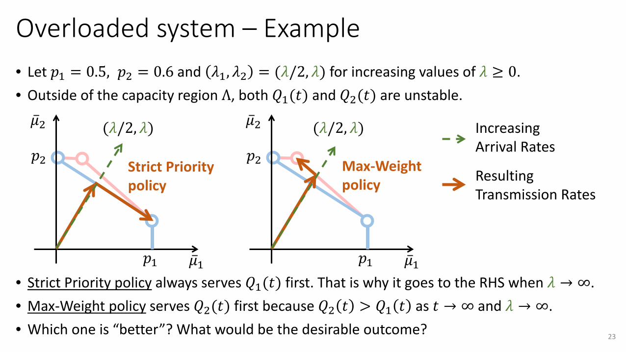
Overloaded system – Example • Let 𝑑𝑑1 = 0.5, 𝑑𝑑2 = 0.6 and 𝜆𝜆1, 𝜆𝜆2 = (𝜆𝜆/2, 𝜆𝜆) for increasing values of 𝜆𝜆 ≥ 0.• Outside of the capacity region Λ, both 𝑄𝑄1(𝑡𝑡) and 𝑄𝑄2(𝑡𝑡) are unstable.

• Strict Priority policy always serves 𝑄𝑄1(𝑡𝑡) first. What happens when 𝜆𝜆 → ∞.• How does the Max-Weight policy behaves?• Which one is “better”? What would be the desirable outcome? 22

�̅�𝜇2

�̅�𝜇1

𝑑𝑑2

𝑑𝑑1

�̅�𝜇2

�̅�𝜇1

𝑑𝑑2

𝑑𝑑1

(𝜆𝜆/2, 𝜆𝜆) (𝜆𝜆/2, 𝜆𝜆)

Max-Weight policy

Increasing Arrival Rates

Resulting Transmission Rates

Strict Prioritypolicy

Overloaded system – Example • Let 𝑑𝑑1 = 0.5, 𝑑𝑑2 = 0.6 and 𝜆𝜆1, 𝜆𝜆2 = (𝜆𝜆/2, 𝜆𝜆) for increasing values of 𝜆𝜆 ≥ 0.• Outside of the capacity region Λ, both 𝑄𝑄1(𝑡𝑡) and 𝑄𝑄2(𝑡𝑡) are unstable.

• Strict Priority policy always serves 𝑄𝑄1(𝑡𝑡) first. That is why it goes to the RHS when 𝜆𝜆 → ∞.• Max-Weight policy serves 𝑄𝑄2(𝑡𝑡) first because 𝑄𝑄2 𝑡𝑡 > 𝑄𝑄1 𝑡𝑡 as 𝑡𝑡 → ∞ and 𝜆𝜆 → ∞.• Which one is “better”? What would be the desirable outcome? 23

�̅�𝜇2

�̅�𝜇1

𝑑𝑑2

𝑑𝑑1

�̅�𝜇2

�̅�𝜇1

𝑑𝑑2

𝑑𝑑1

(𝜆𝜆/2, 𝜆𝜆) (𝜆𝜆/2, 𝜆𝜆)

Max-Weight policy

Increasing Arrival Rates

Resulting Transmission Rates

Strict Prioritypolicy

Overloaded system – Definition• Assume that arrival rates 𝜆𝜆𝑛𝑛𝑐𝑐 are infinitely large. Then all queues 𝑄𝑄𝑛𝑛𝑐𝑐(𝑡𝑡) are unstable.

• Admission Control. Let 𝑎𝑎𝑛𝑛𝑐𝑐(𝑡𝑡) be the number of packets admitted to 𝑄𝑄𝑛𝑛𝑐𝑐(𝑡𝑡) at time 𝑡𝑡.

• Assume that admission is bounded ∑𝑐𝑐=1𝐾𝐾 𝑎𝑎𝑛𝑛𝑐𝑐 𝑡𝑡 ≤ 𝑅𝑅𝑛𝑛𝑚𝑚𝑚𝑚𝑚𝑚 ,∀𝑡𝑡,𝑛𝑛 ;

• Define the time-average admission rate as �̅�𝑎𝑛𝑛𝑐𝑐 ≔ lim𝑡𝑡→∞

1𝑡𝑡∑𝜏𝜏=0𝑡𝑡−1 𝔼𝔼 𝑎𝑎𝑛𝑛𝑐𝑐 𝜏𝜏 ,∀𝑛𝑛, 𝑐𝑐;

• From another perspective: now we can control packet arrivals to the queues 𝑎𝑎𝑛𝑛𝑐𝑐 𝑡𝑡 . Can we utilize admission control to achieve a “desired network behavior”? 24

𝑎𝑎1(𝑡𝑡) 𝜇𝜇1(𝑡𝑡)Arrivals

𝑎𝑎2(𝑡𝑡)𝜇𝜇2(𝑡𝑡)

Arrivals

𝑠𝑠1(𝑡𝑡)

𝑠𝑠2(𝑡𝑡)

𝑄𝑄1(𝑡𝑡)

𝑄𝑄2(𝑡𝑡)

Overloaded system – Utility Function• Let 𝑔𝑔𝑛𝑛𝑐𝑐 𝑎𝑎 be strictly concave, non-decreasing and continuously differentiable.

• Capture satisfaction/utility attained from sending commodity-c at a time-average rate r.

• Can be used to achieve fairness across commodities and nodes.

• Good model for elastic flows (e.g. file download). Not good for inelastic flow or for flows with an intrinsic rate (e.g. real-time video).

• Example: consider a network with 3 nodes, 3 flows and equal link capacities of 1. What is the transmission rate distribution that maximizes:

1) �̅�𝑎12 + �̅�𝑎13 + �̅�𝑎23 ? �̅�𝑎12; �̅�𝑎13; �̅�𝑎23 = 1; 0; 1

2) 𝒞𝒞𝑜𝑜𝑔𝑔 �̅�𝑎12 + 𝒞𝒞𝑜𝑜𝑔𝑔 �̅�𝑎13 + 𝒞𝒞𝑜𝑜𝑔𝑔 �̅�𝑎23 ? Ans. 23

; 13

; 23

3) Max-min fairness ? Ans. 12

; 12

; 12

25

1 2 3

�𝒓𝒓𝟏𝟏𝟐𝟐 �𝒓𝒓𝟐𝟐𝟑𝟑

�𝒓𝒓𝟏𝟏𝟑𝟑

Overloaded system – Goal• Recall that 𝜇𝜇𝑛𝑛,𝑗𝑗

𝑐𝑐 𝑡𝑡 is the offered transmission opportunity over link (𝑛𝑛, 𝑗𝑗) to commodity-𝑐𝑐. Notice that: ∑𝑐𝑐=1𝐾𝐾 𝜇𝜇𝑛𝑛,𝑗𝑗

𝑐𝑐 𝑡𝑡 = 𝜇𝜇𝑛𝑛,𝑗𝑗(𝑡𝑡) is the total offered transmission opportunity.

• With controlled packet arrivals to the queues 𝑎𝑎𝑛𝑛𝑐𝑐 𝑡𝑡 , we have

• Goal is to design admission, routing and scheduling algorithms that solve the optimal sum utility problem:

• Is it possible to use Stationary Randomized Policy? Is it a practical policy?26

max �𝑛𝑛=1

𝑁𝑁

�𝑐𝑐=1

𝐾𝐾

𝑔𝑔𝑛𝑛𝑐𝑐 �̅�𝑎𝑛𝑛𝑐𝑐 𝑠𝑠. 𝑡𝑡. : �̅�𝑎𝑛𝑛𝑐𝑐 𝑛𝑛,𝑐𝑐 ∈ 𝛬𝛬 and �̅�𝑎𝑛𝑛𝑐𝑐 ≥ 0,∀𝑛𝑛, 𝑐𝑐



𝑖𝑖=1

𝑁𝑁𝜇𝜇𝑖𝑖,𝑛𝑛𝑐𝑐 𝑡𝑡 + 𝑎𝑎𝑛𝑛𝑐𝑐 𝑡𝑡

Lyapunov Optimization• Lindley recursion:

• Lyapunov Function:

• One-slot Lyapunov Drift:

• Drift-Plus Penalty (DPP) Function:

• Next, we obtain an upper bound to the DPP Function and derive an algorithm that minimizes this upper bound. By minimizing the upper bound, we aim to achieve low sum of queues backlogs 𝑄𝑄𝑛𝑛𝑐𝑐 𝑡𝑡 and high sum of utility functions 𝑔𝑔𝑛𝑛𝑐𝑐 �̅�𝑎𝑛𝑛𝑐𝑐 . The DPP algorithm is throughput optimal and ensures that utility is arbitrarily close to optimal.

27

Δ 𝑄𝑄 𝑡𝑡 + 𝑉𝑉 𝔼𝔼 −∑𝑛𝑛=1𝑁𝑁 ∑𝑐𝑐=1𝐾𝐾 𝑔𝑔𝑛𝑛𝑐𝑐 𝑎𝑎𝑛𝑛𝑐𝑐 𝑡𝑡 𝑄𝑄(𝑡𝑡)



𝑖𝑖=1

𝑁𝑁𝜇𝜇𝑖𝑖,𝑛𝑛𝑐𝑐 𝑡𝑡 + 𝑎𝑎𝑛𝑛𝑐𝑐 𝑡𝑡

𝐿𝐿 𝑡𝑡 =12�

𝑛𝑛=1

𝑁𝑁�

𝑐𝑐=1

𝐾𝐾𝑄𝑄𝑛𝑛𝑐𝑐 𝑡𝑡

2

Δ 𝑄𝑄 𝑡𝑡 = 𝔼𝔼 𝐿𝐿 𝑡𝑡 + 1 − 𝐿𝐿(𝑡𝑡) 𝑄𝑄(𝑡𝑡)

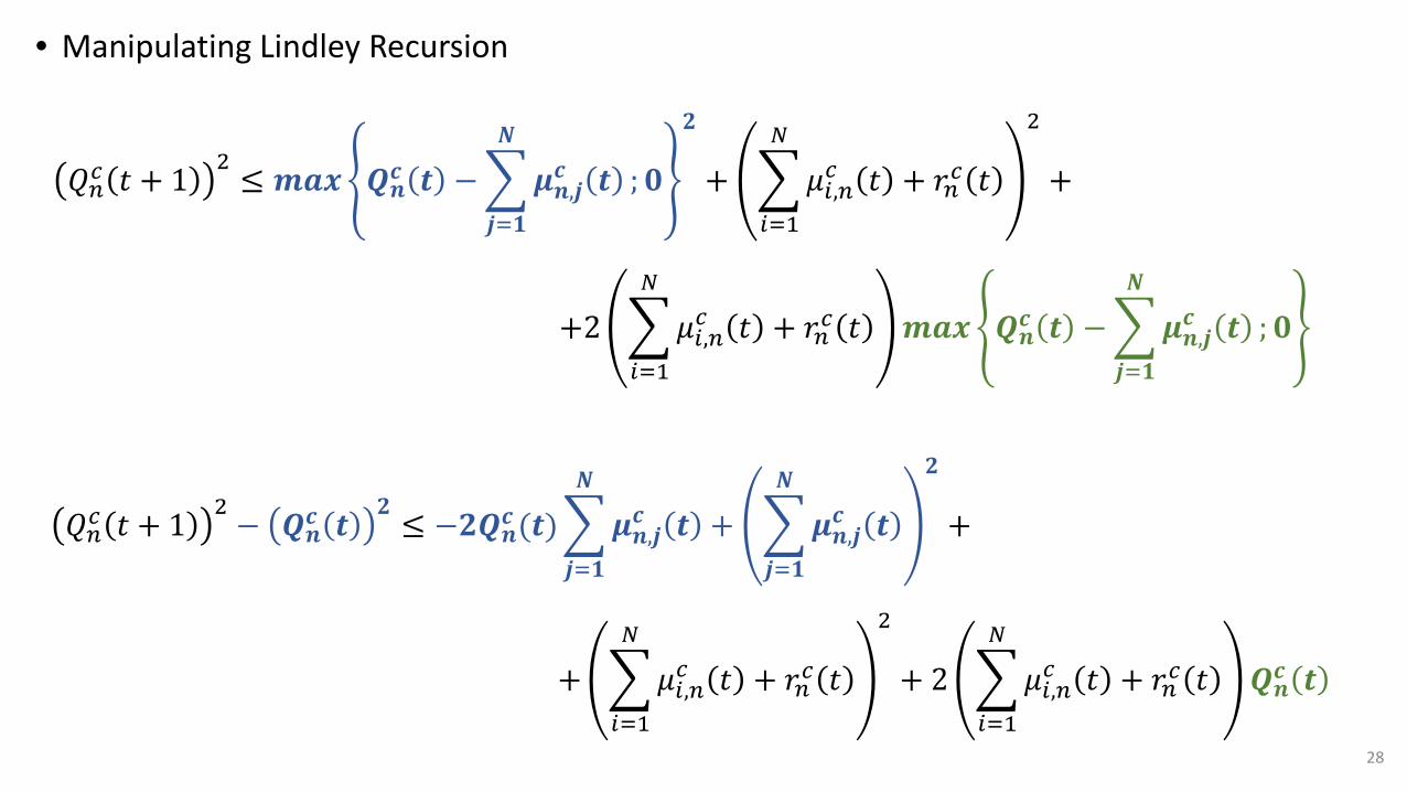
• Manipulating Lindley Recursion

28

𝑄𝑄𝑛𝑛𝑐𝑐 𝑡𝑡 + 12≤ 𝒎𝒎𝒎𝒎𝒎𝒎 𝑸𝑸𝒏𝒏

𝒄𝒄 𝒕𝒕 −�𝒋𝒋=𝟏𝟏

𝑵𝑵

𝝁𝝁𝒏𝒏,𝒋𝒋𝒄𝒄 𝒕𝒕 ;𝟎𝟎

𝟐𝟐

+ �𝑖𝑖=1

𝑁𝑁

𝜇𝜇𝑖𝑖,𝑛𝑛𝑐𝑐 𝑡𝑡 + 𝑎𝑎𝑛𝑛𝑐𝑐 𝑡𝑡

2

+

𝑄𝑄𝑛𝑛𝑐𝑐 𝑡𝑡 + 12− 𝑸𝑸𝒏𝒏

𝒄𝒄 𝒕𝒕𝟐𝟐≤ −𝟐𝟐𝑸𝑸𝒏𝒏

𝒄𝒄 (𝒕𝒕)�𝒋𝒋=𝟏𝟏

𝑵𝑵

𝝁𝝁𝒏𝒏,𝒋𝒋𝒄𝒄 𝒕𝒕 + �

𝒋𝒋=𝟏𝟏

𝑵𝑵

𝝁𝝁𝒏𝒏,𝒋𝒋𝒄𝒄 𝒕𝒕

𝟐𝟐

+

+2 �𝑖𝑖=1

𝑁𝑁

𝜇𝜇𝑖𝑖,𝑛𝑛𝑐𝑐 𝑡𝑡 + 𝑎𝑎𝑛𝑛𝑐𝑐 𝑡𝑡 𝒎𝒎𝒎𝒎𝒎𝒎 𝑸𝑸𝒏𝒏𝒄𝒄 𝒕𝒕 −�

𝒋𝒋=𝟏𝟏

𝑵𝑵

𝝁𝝁𝒏𝒏,𝒋𝒋𝒄𝒄 𝒕𝒕 ;𝟎𝟎

+ �𝑖𝑖=1

𝑁𝑁

𝜇𝜇𝑖𝑖,𝑛𝑛𝑐𝑐 𝑡𝑡 + 𝑎𝑎𝑛𝑛𝑐𝑐 𝑡𝑡

2

+ 2 �𝑖𝑖=1

𝑁𝑁

𝜇𝜇𝑖𝑖,𝑛𝑛𝑐𝑐 𝑡𝑡 + 𝑎𝑎𝑛𝑛𝑐𝑐 𝑡𝑡 𝑸𝑸𝒏𝒏𝒄𝒄 𝒕𝒕

• Substituting into the Lyapunov Drift:

• Assuming that second moments are all bounded, B is a constant. 29

Δ 𝑡𝑡 ≤ −�𝑛𝑛=1

𝑁𝑁

�𝑐𝑐=1

𝐾𝐾

𝑄𝑄𝑛𝑛𝑐𝑐 𝑡𝑡 𝔼𝔼 ∑𝑗𝑗=1𝑁𝑁 𝝁𝝁𝒏𝒏,𝒋𝒋𝒄𝒄 𝒕𝒕 − ∑𝑖𝑖=1𝑁𝑁 𝝁𝝁𝒊𝒊,𝒏𝒏𝒄𝒄 𝒕𝒕 − 𝒓𝒓𝒏𝒏𝒄𝒄 𝒕𝒕 𝑄𝑄 𝑡𝑡 + 𝐵𝐵

𝐵𝐵 ≥12�𝑛𝑛=1

𝑁𝑁

�𝑐𝑐=1

𝐾𝐾

𝔼𝔼 ∑𝑗𝑗=1𝑁𝑁 𝝁𝝁𝒏𝒏,𝒋𝒋𝒄𝒄 𝒕𝒕

2+ ∑𝑖𝑖=1𝑁𝑁 𝝁𝝁𝒊𝒊,𝒏𝒏𝒄𝒄 𝒕𝒕 + 𝒓𝒓𝒏𝒏𝒄𝒄 𝒕𝒕

2𝑄𝑄 𝑡𝑡

𝑄𝑄𝑛𝑛𝑐𝑐 𝑡𝑡 + 12− 𝑄𝑄𝑛𝑛𝑐𝑐 𝑡𝑡

2≤ −2𝑄𝑄𝑛𝑛𝑐𝑐 𝑡𝑡 �

𝑗𝑗=1

𝑁𝑁

𝝁𝝁𝒏𝒏,𝒋𝒋𝒄𝒄 𝒕𝒕 −�

𝑖𝑖=1

𝑁𝑁

𝝁𝝁𝒊𝒊,𝒏𝒏𝒄𝒄 𝒕𝒕 − 𝒓𝒓𝒏𝒏𝒄𝒄 𝒕𝒕 +

+ �𝑗𝑗=1

𝑁𝑁

𝝁𝝁𝒏𝒏,𝒋𝒋𝒄𝒄 𝒕𝒕

2

+ �𝑖𝑖=1

𝑁𝑁

𝝁𝝁𝒊𝒊,𝒏𝒏𝒄𝒄 𝒕𝒕 + 𝒓𝒓𝒏𝒏𝒄𝒄 𝒕𝒕

2

where

Δ 𝑄𝑄 𝑡𝑡 =12�𝑛𝑛=1

𝑁𝑁

�𝑐𝑐=1

𝐾𝐾

𝔼𝔼 𝑄𝑄𝑛𝑛𝑐𝑐 𝑡𝑡 + 12− 𝑄𝑄𝑛𝑛𝑐𝑐 𝑡𝑡

2𝑄𝑄(𝑡𝑡)

• Drift-Plus Penalty: consider the expression Δ 𝑡𝑡 − 𝑉𝑉 𝔼𝔼 ∑𝑛𝑛=1𝑁𝑁 ∑𝑐𝑐=1𝐾𝐾 𝑔𝑔𝑛𝑛𝑐𝑐 𝒓𝒓𝒏𝒏𝒄𝒄 𝒕𝒕 𝑄𝑄(𝑡𝑡)

• DPP algorithm minimizes the upper bound on the RHS at every slot 𝒕𝒕. The minimization can be separated into two sub-problems: i) routing and scheduling 𝝁𝝁𝒊𝒊,𝒋𝒋𝑪𝑪 𝒕𝒕 ; and ii) admission control 𝒓𝒓𝒏𝒏𝒄𝒄 𝒕𝒕 .

30

Δ 𝑡𝑡 − 𝑉𝑉�𝑛𝑛=1

𝑁𝑁

�𝑐𝑐=1

𝐾𝐾

𝔼𝔼 𝑔𝑔𝑛𝑛𝑐𝑐 𝒓𝒓𝒏𝒏𝒄𝒄 𝒕𝒕 𝑄𝑄(𝑡𝑡) ≤ 𝐵𝐵 −�𝑛𝑛=1

𝑁𝑁

�𝑐𝑐=1

𝐾𝐾

𝔼𝔼 𝑄𝑄𝑛𝑛𝑐𝑐 𝑡𝑡 ∑𝑗𝑗=1𝑁𝑁 𝝁𝝁𝒏𝒏,𝒋𝒋𝒄𝒄 𝒕𝒕 − 𝑄𝑄𝑛𝑛𝑐𝑐 𝑡𝑡 ∑𝑖𝑖=1𝑁𝑁 𝝁𝝁𝒊𝒊,𝒏𝒏𝒄𝒄 𝒕𝒕 +

−𝑄𝑄𝑛𝑛𝑐𝑐 𝑡𝑡 𝒓𝒓𝒏𝒏𝒄𝒄 𝒕𝒕 + 𝑉𝑉𝑔𝑔𝑛𝑛𝑐𝑐 𝒓𝒓𝒏𝒏𝒄𝒄 𝒕𝒕 𝑄𝑄 𝑡𝑡


𝑁𝑁

�𝑐𝑐=1

𝐾𝐾


𝑁𝑁

�𝑐𝑐=1

𝐾𝐾

𝑄𝑄𝑛𝑛𝑐𝑐 𝑡𝑡 𝔼𝔼 ∑𝑗𝑗=1𝑁𝑁 𝝁𝝁𝒏𝒏,𝒋𝒋𝒄𝒄 𝒕𝒕 − ∑𝑖𝑖=1𝑁𝑁 𝝁𝝁𝒊𝒊,𝒏𝒏𝒄𝒄 𝒕𝒕 𝑄𝑄 𝑡𝑡 +

−�𝑛𝑛=1

𝑁𝑁

�𝑐𝑐=1

𝐾𝐾

𝔼𝔼 −𝑄𝑄𝑛𝑛𝑐𝑐 𝑡𝑡 𝒓𝒓𝒏𝒏𝒄𝒄 𝒕𝒕 + 𝑉𝑉𝑔𝑔𝑛𝑛𝑐𝑐 𝒓𝒓𝒏𝒏𝒄𝒄 𝒕𝒕 𝑄𝑄 𝑡𝑡

Drift-Plus PenaltyThe DPP minimization can be separated into two sub-problems:

• Routing & Scheduling:

• Admission Control:

31

max𝜇𝜇 𝑡𝑡 ∈Γ

�𝑛𝑛=1

𝑁𝑁

�𝑐𝑐=1

𝐾𝐾

𝑄𝑄𝑛𝑛𝑐𝑐 𝑡𝑡 𝔼𝔼 ∑𝑗𝑗=1𝑁𝑁 𝝁𝝁𝒏𝒏,𝒋𝒋𝒄𝒄 𝒕𝒕 − ∑𝑖𝑖=1𝑁𝑁 𝝁𝝁𝒊𝒊,𝒏𝒏𝒄𝒄 𝒕𝒕 𝑄𝑄 𝑡𝑡

max𝑟𝑟

�𝑛𝑛=1

𝑁𝑁

�𝑐𝑐=1

𝐾𝐾


𝑠𝑠. 𝑡𝑡. :�𝑐𝑐=1

𝐾𝐾

𝒓𝒓𝒏𝒏𝒄𝒄 𝒕𝒕 ≤ 𝑅𝑅𝑛𝑛𝑚𝑚𝑚𝑚𝑚𝑚,∀𝑛𝑛

𝒓𝒓𝒏𝒏𝒄𝒄 𝒕𝒕 ≥ 0,∀𝑛𝑛, 𝑐𝑐

Drift-Plus Penalty – Routing & Scheduling• Routing & Scheduling

32


�𝑛𝑛=1

𝑁𝑁

�𝑐𝑐=1

𝐾𝐾

𝑄𝑄𝑛𝑛𝑐𝑐 𝑡𝑡 𝔼𝔼 ∑𝑗𝑗=1𝑁𝑁 𝝁𝝁𝒏𝒏,𝒋𝒋𝒄𝒄 𝒕𝒕 − ∑𝑖𝑖=1𝑁𝑁 𝝁𝝁𝒊𝒊,𝒏𝒏𝒄𝒄 𝒕𝒕 𝑄𝑄 𝑡𝑡


�𝑛𝑛=1

𝑁𝑁

�𝑐𝑐=1

𝐾𝐾

�𝑗𝑗=1

𝑁𝑁

𝔼𝔼 𝑄𝑄𝑛𝑛𝑐𝑐 𝑡𝑡 𝝁𝝁𝒏𝒏,𝒋𝒋𝒄𝒄 𝒕𝒕 𝑄𝑄 𝑡𝑡 −�

𝑛𝑛=1

𝑁𝑁

�𝑐𝑐=1

𝐾𝐾

�𝑖𝑖=1

𝑁𝑁

𝔼𝔼 𝑄𝑄𝑛𝑛𝑐𝑐 𝑡𝑡 𝝁𝝁𝒊𝒊,𝒏𝒏𝒄𝒄 𝒕𝒕 𝑄𝑄 𝑡𝑡


�𝒊𝒊=𝟏𝟏

𝑁𝑁

�𝑐𝑐=1

𝐾𝐾

�𝑗𝑗=1

𝑁𝑁

𝔼𝔼 𝑄𝑄𝒊𝒊𝑐𝑐 𝑡𝑡 𝝁𝝁𝒊𝒊,𝒋𝒋𝒄𝒄 𝒕𝒕 𝑄𝑄 𝑡𝑡 −�𝒋𝒋=𝟏𝟏

𝑁𝑁

�𝑐𝑐=1

𝐾𝐾

�𝑖𝑖=1

𝑁𝑁

𝔼𝔼 𝑄𝑄𝒋𝒋𝑐𝑐 𝑡𝑡 𝝁𝝁𝒊𝒊,𝒋𝒋𝒄𝒄 𝒕𝒕 𝑄𝑄 𝑡𝑡


�𝑖𝑖=1

𝑁𝑁

�𝑐𝑐=1

𝐾𝐾

�𝑗𝑗=1

𝑁𝑁

𝑄𝑄𝑖𝑖𝑐𝑐 𝑡𝑡 − 𝑄𝑄𝑗𝑗𝑐𝑐 𝑡𝑡 𝔼𝔼 𝝁𝝁𝒊𝒊,𝒋𝒋𝒄𝒄 𝒕𝒕 𝑄𝑄 𝑡𝑡

Drift-Plus Penalty – Routing & SchedulingRouting & Scheduling

Solution [Backpressure – presented in previous lectures]:• Routing: at time 𝑡𝑡 and for every link (𝑖𝑖, 𝑗𝑗), select the commodity with highest differential

backlog, namely 𝑐𝑐𝑖𝑖,𝑗𝑗∗ = argmax 𝑄𝑄𝑖𝑖𝑐𝑐 𝑡𝑡 − 𝑄𝑄𝑗𝑗𝑐𝑐 𝑡𝑡

• Scheduling: for a given state 𝑠𝑠 𝑡𝑡 = 𝑠𝑠, select action 𝐼𝐼 𝑡𝑡 = 𝐼𝐼 such that the set of

transmission rates 𝑼𝑼 𝑠𝑠, 𝐼𝐼 = 𝝁𝝁𝒊𝒊,𝒋𝒋 𝒕𝒕 𝑖𝑖,𝑗𝑗yields maximum sum:

�(𝑖𝑖,𝑗𝑗)

𝑄𝑄𝑖𝑖𝑐𝑐𝑖𝑖,𝑗𝑗∗

𝑡𝑡 − 𝑄𝑄𝑗𝑗𝑐𝑐𝑖𝑖,𝑗𝑗∗

𝑡𝑡 𝝁𝝁𝒊𝒊,𝒋𝒋 𝒕𝒕

Notice that full rate is allocated to commodity 𝑐𝑐𝑖𝑖,𝑗𝑗∗ , namely 𝝁𝝁𝒊𝒊,𝒋𝒋 𝒕𝒕 = 𝝁𝝁𝒊𝒊,𝒋𝒋𝒄𝒄𝒊𝒊,𝒋𝒋∗

𝒕𝒕 .33


�𝑖𝑖=1

𝑁𝑁

�𝑐𝑐=1

𝐾𝐾

�𝑗𝑗=1

𝑁𝑁

𝑄𝑄𝑖𝑖𝑐𝑐 𝑡𝑡 − 𝑄𝑄𝑗𝑗𝑐𝑐 𝑡𝑡 𝔼𝔼 𝝁𝝁𝒊𝒊,𝒋𝒋𝒄𝒄 𝒕𝒕 𝑄𝑄 𝑡𝑡

Drift-Plus Penalty – Admission Control• Admission Control

• Maximization is separable into a per-node problem. At time 𝑡𝑡, each node 𝑛𝑛 should select the set of values 𝒓𝒓𝒏𝒏𝒄𝒄 𝒕𝒕 ,∀𝑐𝑐, that solve the problem:

Each node solves the problem independently of other nodes. The objective function is concave and constraints are linear. How to solve?

34

max𝑟𝑟

�𝑛𝑛=1

𝑁𝑁

�𝑐𝑐=1

𝐾𝐾

𝔼𝔼 −𝑄𝑄𝑛𝑛𝑐𝑐 𝑡𝑡 𝒓𝒓𝒏𝒏𝒄𝒄 𝒕𝒕 + 𝑉𝑉𝑔𝑔𝑛𝑛𝑐𝑐 𝒓𝒓𝒏𝒏𝒄𝒄 𝒕𝒕 𝑄𝑄 𝑡𝑡 𝑠𝑠. 𝑡𝑡. :�𝑐𝑐=1

𝐾𝐾

𝒓𝒓𝒏𝒏𝒄𝒄 𝒕𝒕 ≤ 𝑅𝑅𝑛𝑛𝑚𝑚𝑚𝑚𝑚𝑚,∀𝑛𝑛


max𝑟𝑟𝑛𝑛𝑐𝑐(𝑡𝑡)

�𝑐𝑐=1

𝐾𝐾

𝑉𝑉𝑔𝑔𝑛𝑛𝑐𝑐 𝒓𝒓𝒏𝒏𝒄𝒄 𝒕𝒕 − 𝑄𝑄𝑛𝑛𝑐𝑐 𝑡𝑡 𝒓𝒓𝒏𝒏𝒄𝒄 𝒕𝒕 𝑠𝑠. 𝑡𝑡. :�𝑐𝑐=1

𝐾𝐾

𝒓𝒓𝒏𝒏𝒄𝒄 𝒕𝒕 ≤ 𝑅𝑅𝑛𝑛𝑚𝑚𝑚𝑚𝑚𝑚


Drift-Plus Penalty – KKT Conditions• Lagrangean:

where 𝜂𝜂 and 𝛾𝛾𝑐𝑐 are non-negative KKT multipliers. The KKT Conditions can be written as:

(Stationarity)

(Complementary Slackness) and

(Primal/Dual Feasibility)

35

𝛻𝛻𝒓𝒓𝒏𝒏𝒄𝒄 (𝒕𝒕)ℒ . = 𝑉𝑉 𝑔𝑔𝑛𝑛𝑐𝑐 𝒓𝒓𝒏𝒏𝒄𝒄 𝒕𝒕 ′ − 𝑄𝑄𝑛𝑛𝑐𝑐 𝑡𝑡 − 𝜂𝜂 + 𝛾𝛾𝑐𝑐 = 0

𝜂𝜂 �𝑐𝑐=1

𝐾𝐾𝒓𝒓𝒏𝒏𝒄𝒄 𝒕𝒕 − 𝑅𝑅𝑛𝑛𝑚𝑚𝑚𝑚𝑚𝑚 = 0 𝛾𝛾𝑐𝑐𝒓𝒓𝒏𝒏𝒄𝒄 𝒕𝒕 = 0,∀𝑐𝑐

ℒ 𝒓𝒓𝒏𝒏𝒄𝒄 𝒕𝒕 , 𝜂𝜂, 𝛾𝛾𝑐𝑐 = �𝑐𝑐=1

𝐾𝐾

𝑉𝑉𝑔𝑔𝑛𝑛𝑐𝑐 𝒓𝒓𝒏𝒏𝒄𝒄 𝒕𝒕 − 𝑄𝑄𝑛𝑛𝑐𝑐 𝑡𝑡 𝒓𝒓𝒏𝒏𝒄𝒄 𝒕𝒕 − 𝜂𝜂 �𝑐𝑐=1

𝐾𝐾

𝒓𝒓𝒏𝒏𝒄𝒄 𝒕𝒕 − 𝑅𝑅𝑛𝑛𝑚𝑚𝑚𝑚𝑚𝑚 + �𝑐𝑐=1

𝐾𝐾

𝛾𝛾𝑐𝑐𝒓𝒓𝒏𝒏𝒄𝒄 𝒕𝒕

�𝑐𝑐=1

𝐾𝐾

𝒓𝒓𝒏𝒏𝒄𝒄 𝒕𝒕 ≤ 𝑅𝑅𝑛𝑛𝑚𝑚𝑚𝑚𝑚𝑚 and 𝒓𝒓𝒏𝒏𝒄𝒄 𝒕𝒕 ≥ 0,∀𝑐𝑐 and 𝜂𝜂 ≥ 0 and 𝛾𝛾𝑐𝑐 ≥ 0,∀𝑐𝑐

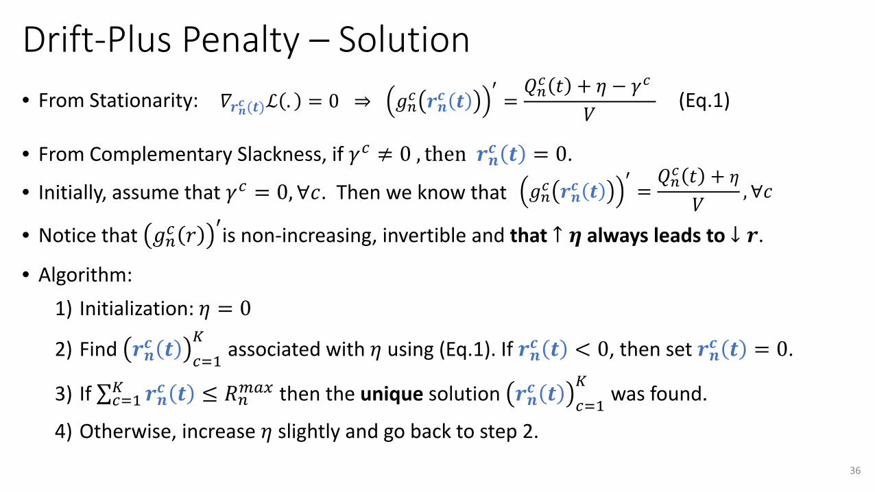
Drift-Plus Penalty – Solution• From Stationarity: (Eq.1)

• From Complementary Slackness, if 𝛾𝛾𝑐𝑐 ≠ 0 , then 𝒓𝒓𝒏𝒏𝒄𝒄 𝒕𝒕 = 0.

• Initially, assume that 𝛾𝛾𝑐𝑐 = 0,∀𝑐𝑐. Then we know that

• Notice that 𝑔𝑔𝑛𝑛𝑐𝑐 𝑎𝑎′is non-increasing, invertible and that ↑ 𝜼𝜼 always leads to ↓ 𝒓𝒓.

• Algorithm: 1) Initialization: 𝜂𝜂 = 0

2) Find 𝒓𝒓𝒏𝒏𝒄𝒄 𝒕𝒕 𝑐𝑐=1𝐾𝐾

associated with 𝜂𝜂 using (Eq.1). If 𝒓𝒓𝒏𝒏𝒄𝒄 𝒕𝒕 < 0, then set 𝒓𝒓𝒏𝒏𝒄𝒄 𝒕𝒕 = 0.

3) If ∑𝑐𝑐=1𝐾𝐾 𝒓𝒓𝒏𝒏𝒄𝒄 𝒕𝒕 ≤ 𝑅𝑅𝑛𝑛𝑚𝑚𝑚𝑚𝑚𝑚 then the unique solution 𝒓𝒓𝒏𝒏𝒄𝒄 𝒕𝒕 𝑐𝑐=1𝐾𝐾

was found.

4) Otherwise, increase 𝜂𝜂 slightly and go back to step 2.

36

𝛻𝛻𝒓𝒓𝒏𝒏𝒄𝒄 (𝒕𝒕)ℒ . = 0 ⇒ 𝑔𝑔𝑛𝑛𝑐𝑐 𝒓𝒓𝒏𝒏𝒄𝒄 𝒕𝒕′

=𝑄𝑄𝑛𝑛𝑐𝑐 𝑡𝑡 + 𝜂𝜂 − 𝛾𝛾𝑐𝑐

𝑉𝑉

𝑔𝑔𝑛𝑛𝑐𝑐 𝒓𝒓𝒏𝒏𝒄𝒄 𝒕𝒕′

=𝑄𝑄𝑛𝑛𝑐𝑐 𝑡𝑡 + 𝜂𝜂

𝑉𝑉,∀𝑐𝑐

Drift-Plus Penalty – Solution (Example)Example: consider the utility function 𝑔𝑔𝑛𝑛𝑐𝑐 𝒓𝒓𝒏𝒏𝒄𝒄 𝒕𝒕 = log 𝒓𝒓𝒏𝒏𝒄𝒄 𝒕𝒕 .

• Then

• Assuming 𝜂𝜂 = 𝛾𝛾𝑐𝑐 = 0 and that 𝑅𝑅𝑛𝑛𝑚𝑚𝑚𝑚𝑚𝑚 is large enough, the solution is:

• Notice that:

• A larger backlog on the queue ↑ Qnc (t) leads to less packets being admitted to the

queue ↓ 𝐫𝐫𝐧𝐧𝐜𝐜 𝐭𝐭 , what makes sense.• Larger V implies in larger 𝐫𝐫𝐧𝐧𝐜𝐜 𝐭𝐭 which, in turn, implies in more network congestion.

37

𝑔𝑔𝑛𝑛𝑐𝑐 𝒓𝒓𝒏𝒏𝒄𝒄 𝒕𝒕′

=1

𝒓𝒓𝒏𝒏𝒄𝒄 𝒕𝒕=𝑄𝑄𝑛𝑛𝑐𝑐 𝑡𝑡 + 𝜂𝜂 − 𝛾𝛾𝑐𝑐

𝑉𝑉→ 𝒓𝒓𝒏𝒏𝒄𝒄 𝒕𝒕 =

𝑉𝑉𝑄𝑄𝑛𝑛𝑐𝑐 𝑡𝑡 + 𝜂𝜂 − 𝛾𝛾𝑐𝑐

,∀𝑛𝑛, 𝑐𝑐, 𝑡𝑡

𝒓𝒓𝒏𝒏𝒄𝒄 𝒕𝒕 =𝑉𝑉

𝑄𝑄𝑛𝑛𝑐𝑐 𝑡𝑡,∀𝑛𝑛, 𝑐𝑐, 𝑡𝑡

Drift-Plus Penalty AlgorithmAt every time t, the DPP algorithm runs three steps:

• Routing: for every link (𝑖𝑖, 𝑗𝑗), select the commodity with highest differential backlog, namely 𝑐𝑐𝑖𝑖,𝑗𝑗∗ = argmax 𝑄𝑄𝑖𝑖𝑐𝑐 𝑡𝑡 − 𝑄𝑄𝑗𝑗𝑐𝑐 𝑡𝑡

• Scheduling: for a given state 𝑠𝑠 𝑡𝑡 = 𝑠𝑠, select action 𝐼𝐼 𝑡𝑡 = 𝐼𝐼 such that the set of transmission rates 𝑼𝑼 𝑠𝑠, 𝐼𝐼 = 𝝁𝝁𝒊𝒊,𝒋𝒋 𝒕𝒕 𝑖𝑖,𝑗𝑗

yields maximum sum:

�(𝑖𝑖,𝑗𝑗)

𝑄𝑄𝑖𝑖𝑐𝑐𝑖𝑖,𝑗𝑗∗

𝑡𝑡 − 𝑄𝑄𝑗𝑗𝑐𝑐𝑖𝑖,𝑗𝑗∗

𝑡𝑡 𝝁𝝁𝒊𝒊,𝒋𝒋 𝒕𝒕

• Admission control: each node 𝑛𝑛 uses its own KKT Conditions to attain the values of 𝒓𝒓𝒏𝒏𝒄𝒄 (𝒕𝒕)which solve:

38

max𝒓𝒓𝒏𝒏𝒄𝒄 (𝒕𝒕)

�𝑐𝑐=1

𝐾𝐾

𝑉𝑉𝑔𝑔𝑛𝑛𝑐𝑐 𝒓𝒓𝒏𝒏𝒄𝒄 𝒕𝒕 − 𝑄𝑄𝑛𝑛𝑐𝑐 𝑡𝑡 𝒓𝒓𝒏𝒏𝒄𝒄 𝒕𝒕 𝑠𝑠. 𝑡𝑡. :�𝑐𝑐=1

𝐾𝐾

𝒓𝒓𝒏𝒏𝒄𝒄 𝒕𝒕 ≤ 𝑅𝑅𝑛𝑛𝑚𝑚𝑚𝑚𝑚𝑚 ; 𝒓𝒓𝒏𝒏𝒄𝒄 𝒕𝒕 ≥ 0,∀𝑛𝑛, 𝑐𝑐

Drift-Plus Penalty Algorithm• Admission Control. The parameter V captures the emphasis on utility maximization. If V is

large, then the admitted rates tend to be large, thus increasing the utility, but at the same time increasing the network delay caused by congestion. Notice that admission control on node 𝑛𝑛 only requires information available locally.

• Routing & Scheduling is done using the Backpressure policy (already discussed in previous lectures). Recall that routing requires no pre-specified paths, since paths are learned dynamically. Moreover, this algorithm does not need information about arrival rates or channel state statistics.

• Next, we show that the DPP Algorithm is throughput optimal and ensures that utility is arbitrarily close to optimal.

39

Performance Analysis – Randomized Policy• Prior to analyzing the performance of the DPP algorithm, we assess the Stationary

Randomized Policy associated with our original utility maximization problem:

• Denote �𝒓𝒓𝒏𝒏𝒄𝒄∗ 𝑛𝑛,𝑐𝑐 as the optimal solution to the utility maximization. A simple admission control algorithm that achieves the optimal solution is: �𝒓𝒓𝒏𝒏𝒄𝒄∗ = 𝑎𝑎𝑛𝑛𝑐𝑐 𝑡𝑡 ,∀𝑡𝑡.

• We know from our discussion of the capacity region that for �𝒓𝒓𝒏𝒏𝒄𝒄∗ 𝑛𝑛,𝑐𝑐 ∈ Λ, there exists flow variables ̅𝑓𝑓𝑖𝑖,𝑗𝑗𝑐𝑐 such that �𝒓𝒓𝒏𝒏𝒄𝒄∗ + ∑𝑖𝑖=1𝑁𝑁 ̅𝑓𝑓𝑖𝑖,𝑛𝑛𝑐𝑐 = ∑𝑗𝑗=1𝑁𝑁 ̅𝑓𝑓𝑛𝑛,𝑗𝑗

𝑐𝑐 and a Stationary Randomized Policy with time-average packet transmission rates �𝝁𝝁𝒊𝒊,𝒋𝒋𝒄𝒄 such that ̅𝑓𝑓𝑖𝑖,𝑗𝑗𝑐𝑐 ≤ �𝝁𝝁𝒊𝒊,𝒋𝒋𝒄𝒄 ,∀𝑖𝑖, 𝑗𝑗, 𝑐𝑐.

• Consider the Stationary Randomized Policy with rates �𝝁𝝁𝒊𝒊,𝒋𝒋𝒄𝒄 = ̅𝑓𝑓𝑖𝑖,𝑗𝑗𝑐𝑐 ,∀𝑖𝑖, 𝑗𝑗, 𝑐𝑐.40

max �𝑛𝑛=1

𝑁𝑁

�𝑐𝑐=1

𝐾𝐾

𝑔𝑔𝑛𝑛𝑐𝑐 �𝒓𝒓𝒏𝒏𝒄𝒄 𝑠𝑠. 𝑡𝑡. : �𝒓𝒓𝒏𝒏𝒄𝒄 𝑛𝑛,𝑐𝑐 ∈ 𝛬𝛬 and �𝒓𝒓𝒏𝒏𝒄𝒄 ≥ 0,∀𝑛𝑛, 𝑐𝑐

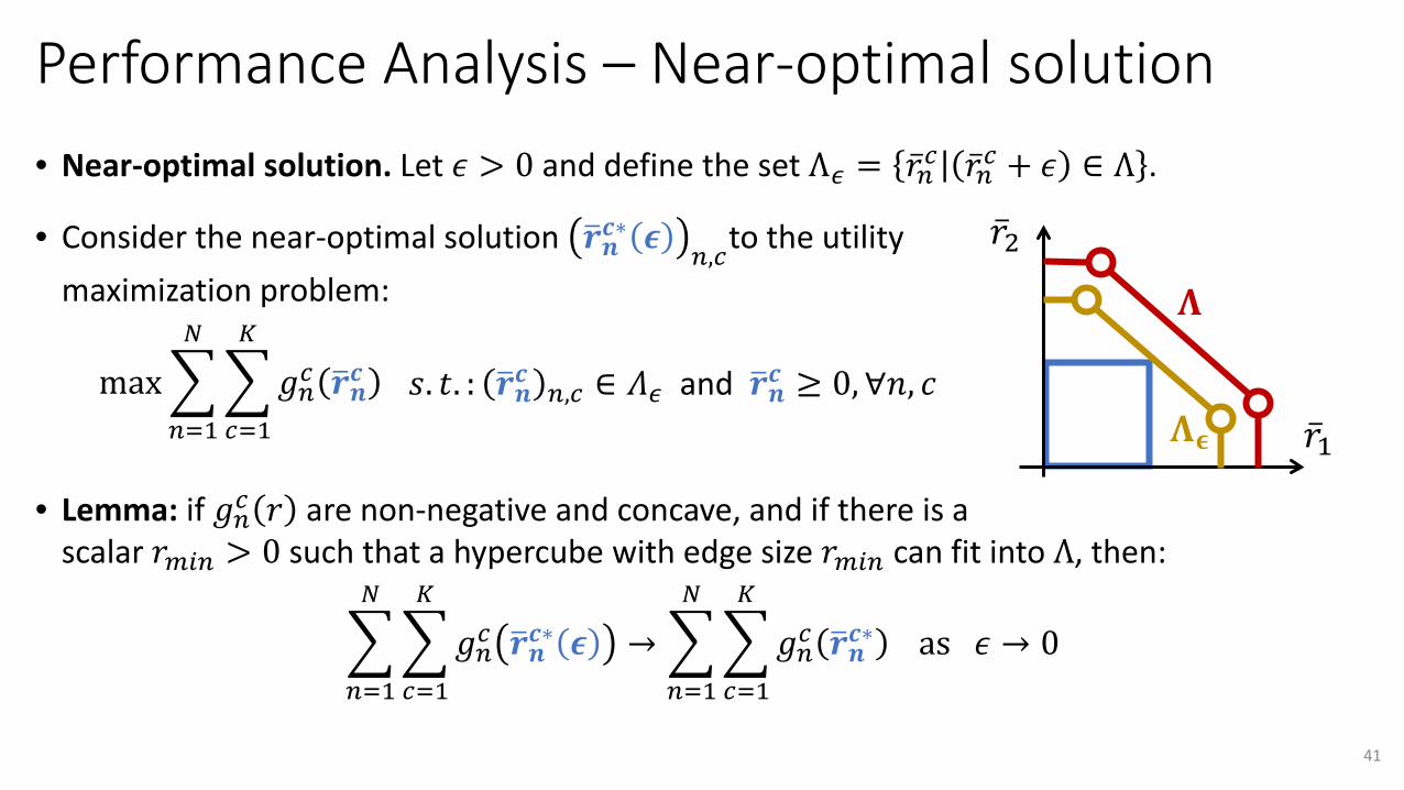
• Near-optimal solution. Let 𝜖𝜖 > 0 and define the set Λ𝜖𝜖 = �̅�𝑎𝑛𝑛𝑐𝑐 �̅�𝑎𝑛𝑛𝑐𝑐 + 𝜖𝜖 ∈ Λ .

• Consider the near-optimal solution �𝒓𝒓𝒏𝒏𝒄𝒄∗ 𝝐𝝐 𝑛𝑛,𝑐𝑐to the utility maximization problem:

• Lemma: if 𝑔𝑔𝑛𝑛𝑐𝑐 𝑎𝑎 are non-negative and concave, and if there is a scalar 𝑎𝑎𝑚𝑚𝑖𝑖𝑛𝑛 > 0 such that a hypercube with edge size 𝑎𝑎𝑚𝑚𝑖𝑖𝑛𝑛 can fit into Λ, then:

�𝑛𝑛=1

𝑁𝑁

�𝑐𝑐=1

𝐾𝐾

𝑔𝑔𝑛𝑛𝑐𝑐 �𝒓𝒓𝒏𝒏𝒄𝒄∗ 𝝐𝝐 → �𝑛𝑛=1

𝑁𝑁

�𝑐𝑐=1

𝐾𝐾

𝑔𝑔𝑛𝑛𝑐𝑐 �𝒓𝒓𝒏𝒏𝒄𝒄∗ as 𝜖𝜖 → 0

Performance Analysis – Near-optimal solution

41

max �𝑛𝑛=1

𝑁𝑁

�𝑐𝑐=1

𝐾𝐾

𝑔𝑔𝑛𝑛𝑐𝑐 �𝒓𝒓𝒏𝒏𝒄𝒄 𝑠𝑠. 𝑡𝑡. : �𝒓𝒓𝒏𝒏𝒄𝒄 𝑛𝑛,𝑐𝑐 ∈ 𝛬𝛬𝜖𝜖 and �𝒓𝒓𝒏𝒏𝒄𝒄 ≥ 0,∀𝑛𝑛, 𝑐𝑐�̅�𝑎1

�̅�𝑎2

𝚲𝚲𝛜𝛜

𝚲𝚲

• Near-optimal solution. Let 𝜖𝜖 > 0 and define the set Λ𝜖𝜖 = �̅�𝑎𝑛𝑛𝑐𝑐 �̅�𝑎𝑛𝑛𝑐𝑐 + 𝜖𝜖 ∈ Λ .

• Consider the near-optimal solution �𝒓𝒓𝒏𝒏𝒄𝒄∗ 𝝐𝝐 𝑛𝑛,𝑐𝑐to the utility maximization problem:

• Consider the Stationary Randomized Policy: �̅�𝑎𝑛𝑛𝑐𝑐 𝑡𝑡 = �𝒓𝒓𝒏𝒏𝒄𝒄∗ 𝝐𝝐 ,∀𝑛𝑛, 𝑐𝑐, 𝑡𝑡 and �𝝁𝝁𝒊𝒊,𝒋𝒋𝒄𝒄 = ̅𝑓𝑓𝑖𝑖,𝑗𝑗𝑐𝑐 ,∀𝑖𝑖, 𝑗𝑗, 𝑐𝑐. Recall that ∑𝑖𝑖=1𝑁𝑁 ̅𝑓𝑓𝑖𝑖,𝑛𝑛𝑐𝑐 + �𝒓𝒓𝒏𝒏𝒄𝒄∗ = ∑𝑗𝑗=1𝑁𝑁 ̅𝑓𝑓𝑛𝑛,𝑗𝑗

𝑐𝑐 . Hence, it follows that:

�𝑖𝑖=1

𝑁𝑁�𝝁𝝁𝒊𝒊,𝒏𝒏𝒄𝒄 + �𝒓𝒓𝒏𝒏𝒄𝒄∗ 𝝐𝝐 + 𝜖𝜖 ≤�

𝑗𝑗=1

𝑁𝑁�𝝁𝝁𝒏𝒏,𝒋𝒋𝒄𝒄 ⇒�

𝑗𝑗=1

𝑁𝑁�𝝁𝝁𝒏𝒏,𝒋𝒋𝒄𝒄 −�

𝑖𝑖=1

𝑁𝑁�𝝁𝝁𝒊𝒊,𝒏𝒏𝒄𝒄 − �𝒓𝒓𝒏𝒏𝒄𝒄∗ 𝝐𝝐 ≥ 𝜖𝜖 > 0

• Next, we compare the drift of the DPP algorithm with the drift of the Randomized Policy.

Performance Analysis – Randomized Policy

42

max �𝑛𝑛=1

𝑁𝑁

�𝑐𝑐=1

𝐾𝐾

𝑔𝑔𝑛𝑛𝑐𝑐 �𝒓𝒓𝒏𝒏𝒄𝒄 𝑠𝑠. 𝑡𝑡. : �𝒓𝒓𝒏𝒏𝒄𝒄 𝑛𝑛,𝑐𝑐 ∈ 𝛬𝛬𝜖𝜖 and �𝒓𝒓𝒏𝒏𝒄𝒄 ≥ 0,∀𝑛𝑛, 𝑐𝑐�̅�𝑎1

�̅�𝑎2

𝚲𝚲𝛜𝛜

𝚲𝚲

(Eq2)

Performance Analysis – DPP Algorithm• Recall the expression for the Drift-Plus Penalty:

• By definition, this upper bound is minimizes by the DPP Algorithm. Hence, the Stationary Randomized Policy achieves a larger upper bound. Substituting �𝝁𝝁𝒊𝒊,𝒋𝒋𝒄𝒄 and �𝒓𝒓𝒏𝒏𝒄𝒄∗ 𝝐𝝐 :

43


𝑁𝑁

�𝑐𝑐=1

𝐾𝐾


𝑁𝑁

�𝑐𝑐=1

𝐾𝐾

𝑄𝑄𝑛𝑛𝑐𝑐 𝑡𝑡 𝔼𝔼 ∑𝑗𝑗=1𝑁𝑁 𝝁𝝁𝒏𝒏,𝒋𝒋𝒄𝒄 𝒕𝒕 − ∑𝑖𝑖=1𝑁𝑁 𝝁𝝁𝒊𝒊,𝒏𝒏𝒄𝒄 𝒕𝒕 𝑄𝑄 𝑡𝑡 +

−�𝑛𝑛=1

𝑁𝑁

�𝑐𝑐=1

𝐾𝐾



𝑁𝑁

�𝑐𝑐=1

𝐾𝐾


𝑁𝑁

�𝑐𝑐=1

𝐾𝐾

𝑄𝑄𝑛𝑛𝑐𝑐 𝑡𝑡 �𝑗𝑗=1

𝑁𝑁

�𝝁𝝁𝒏𝒏,𝒋𝒋𝒄𝒄 −�

𝑖𝑖=1

𝑁𝑁

�𝝁𝝁𝒏𝒏,𝒋𝒋𝒄𝒄 +

−�𝑛𝑛=1

𝑁𝑁

�𝑐𝑐=1

𝐾𝐾

−𝑄𝑄𝑛𝑛𝑐𝑐 𝑡𝑡 �𝒓𝒓𝒏𝒏𝒄𝒄∗ 𝝐𝝐 + 𝑉𝑉𝑔𝑔𝑛𝑛𝑐𝑐 �𝒓𝒓𝒏𝒏𝒄𝒄∗ 𝝐𝝐

• By rearranging the upper bound and utilizing (Eq.2), we have:

• Taking the expectation w.r.t 𝑄𝑄𝑛𝑛𝑐𝑐(𝑡𝑡) and using the definition of Lyapunov Drift:

• Summing over 𝑡𝑡 ∈ 0,2, … ,𝑇𝑇 − 1 and dividing by T gives:

44


𝑁𝑁

�𝑐𝑐=1

𝐾𝐾

𝔼𝔼 𝑔𝑔𝑛𝑛𝑐𝑐 𝒓𝒓𝒏𝒏𝒄𝒄 𝒕𝒕 𝑄𝑄(𝑡𝑡) ≤ 𝐵𝐵 − 𝜖𝜖�𝑛𝑛=1

𝑁𝑁

�𝑐𝑐=1

𝐾𝐾

𝑄𝑄𝑛𝑛𝑐𝑐 𝑡𝑡 −�𝑛𝑛=1

𝑁𝑁

�𝑐𝑐=1

𝐾𝐾

𝑉𝑉𝑔𝑔𝑛𝑛𝑐𝑐 �𝒓𝒓𝒏𝒏𝒄𝒄∗ 𝝐𝝐

𝔼𝔼 𝐿𝐿 𝑡𝑡 + 1 − 𝔼𝔼 𝐿𝐿 𝑡𝑡 − 𝑉𝑉�𝑛𝑛=1

𝑁𝑁

�𝑐𝑐=1

𝐾𝐾

𝔼𝔼 𝑔𝑔𝑛𝑛𝑐𝑐 𝒓𝒓𝒏𝒏𝒄𝒄 𝒕𝒕 ≤ 𝐵𝐵 − 𝜖𝜖�𝑛𝑛=1

𝑁𝑁

�𝑐𝑐=1

𝐾𝐾

𝔼𝔼 𝑄𝑄𝑛𝑛𝑐𝑐 𝑡𝑡 − 𝑉𝑉�𝑛𝑛=1

𝑁𝑁

�𝑐𝑐=1

𝐾𝐾

𝔼𝔼 𝑔𝑔𝑛𝑛𝑐𝑐 �𝒓𝒓𝒏𝒏𝒄𝒄∗ 𝝐𝝐

𝔼𝔼 𝐿𝐿 𝑇𝑇𝑇𝑇

−𝔼𝔼 𝐿𝐿 0

𝑇𝑇−𝑉𝑉𝑇𝑇�𝑡𝑡=0

𝑇𝑇−1

�𝑛𝑛=1

𝑁𝑁

�𝑐𝑐=1

𝐾𝐾

𝔼𝔼 𝑔𝑔𝑛𝑛𝑐𝑐 𝒓𝒓𝒏𝒏𝒄𝒄 𝒕𝒕 ≤

≤ 𝐵𝐵 −𝜖𝜖𝑇𝑇�𝑡𝑡=0

𝑇𝑇−1

�𝑛𝑛=1

𝑁𝑁

�𝑐𝑐=1

𝐾𝐾

𝔼𝔼 𝑄𝑄𝑛𝑛𝑐𝑐 𝑡𝑡 − 𝑉𝑉�𝑛𝑛=1

𝑁𝑁

�𝑐𝑐=1

𝐾𝐾


• Rearranging the expression and knowing that 𝔼𝔼 𝐿𝐿 𝑇𝑇 /𝑇𝑇 is non-negative:

• Taking the limit 𝑇𝑇 → ∞ and assuming that 𝔼𝔼 𝐿𝐿 0 is finite gives:

• Conclusion 1:

• All queues 𝑸𝑸𝒏𝒏𝒄𝒄 𝒕𝒕 are strongly stable. DPP algorithm is throughput optimal.

45

𝜖𝜖𝑇𝑇�𝑡𝑡=0

𝑇𝑇−1

�𝑛𝑛=1

𝑁𝑁

�𝑐𝑐=1

𝐾𝐾

𝔼𝔼 𝑄𝑄𝑛𝑛𝑐𝑐 𝑡𝑡 −𝑉𝑉𝑇𝑇�𝑡𝑡=0

𝑇𝑇−1

�𝑛𝑛=1

𝑁𝑁

�𝑐𝑐=1

𝐾𝐾

𝔼𝔼 𝑔𝑔𝑛𝑛𝑐𝑐 𝒓𝒓𝒏𝒏𝒄𝒄 𝒕𝒕 ≤ 𝐵𝐵 − 𝑉𝑉�𝑛𝑛=1

𝑁𝑁

�𝑐𝑐=1

𝐾𝐾

𝔼𝔼 𝑔𝑔𝑛𝑛𝑐𝑐 �𝒓𝒓𝒏𝒏𝒄𝒄∗ 𝝐𝝐 +𝔼𝔼 𝐿𝐿 0

𝑇𝑇

�𝑛𝑛=1

𝑁𝑁

�𝑐𝑐=1

𝐾𝐾

lim𝑇𝑇→∞

𝜖𝜖𝑇𝑇�𝑡𝑡=0

𝑇𝑇−1

𝔼𝔼 𝑄𝑄𝑛𝑛𝑐𝑐 𝑡𝑡 −�𝑛𝑛=1

𝑁𝑁

�𝑐𝑐=1

𝐾𝐾

lim𝑇𝑇→∞

𝑉𝑉𝑇𝑇�𝑡𝑡=0

𝑇𝑇−1

𝔼𝔼 𝑔𝑔𝑛𝑛𝑐𝑐 𝒓𝒓𝒏𝒏𝒄𝒄 𝒕𝒕 ≤ 𝐵𝐵 − 𝑉𝑉�𝑛𝑛=1

𝑁𝑁

�𝑐𝑐=1

𝐾𝐾


�𝑛𝑛=1

𝑁𝑁

�𝑐𝑐=1

𝐾𝐾

lim𝑇𝑇→∞

1𝑇𝑇�𝑡𝑡=0

𝑇𝑇−1

𝔼𝔼 𝑄𝑄𝑛𝑛𝑐𝑐 𝑡𝑡 ≤𝐵𝐵𝜖𝜖

+𝑉𝑉𝜖𝜖�𝑛𝑛=1

𝑁𝑁

�𝑐𝑐=1

𝐾𝐾

lim𝑇𝑇→∞


𝑇𝑇−1

𝔼𝔼 𝑔𝑔𝑛𝑛𝑐𝑐 𝒓𝒓𝒏𝒏𝒄𝒄 𝒕𝒕 − 𝔼𝔼 𝑔𝑔𝑛𝑛𝑐𝑐 �𝒓𝒓𝒏𝒏𝒄𝒄∗ 𝝐𝝐 < ∞

• On the other hand:

• By Jensen’s inequality and by concavity and continuity of 𝑔𝑔𝑛𝑛𝑐𝑐 𝒓𝒓𝒏𝒏𝒄𝒄 𝒕𝒕 , we have:

• Conclusion 2: For 𝜖𝜖 → 0 :

• Larger values of 𝑽𝑽 take the DPP Algorithm arbitrarily close to the optimal utility.46

�𝑛𝑛=1

𝑁𝑁

�𝑐𝑐=1

𝐾𝐾

lim𝑇𝑇→∞


𝑇𝑇−1

𝔼𝔼 𝑔𝑔𝑛𝑛𝑐𝑐 𝒓𝒓𝒏𝒏𝒄𝒄 𝒕𝒕 ≥ �𝑛𝑛=1

𝑁𝑁

�𝑐𝑐=1

𝐾𝐾

𝔼𝔼 𝑔𝑔𝑛𝑛𝑐𝑐 �𝒓𝒓𝒏𝒏𝒄𝒄∗ 𝝐𝝐 −𝐵𝐵𝑉𝑉

�𝑛𝑛=1

𝑁𝑁

�𝑐𝑐=1

𝐾𝐾

lim𝑇𝑇→∞

𝑔𝑔𝑛𝑛𝑐𝑐1𝑇𝑇�𝑡𝑡=0

𝑇𝑇−1

𝔼𝔼 𝒓𝒓𝒏𝒏𝒄𝒄 𝒕𝒕 ≥ �𝑛𝑛=1

𝑁𝑁

�𝑐𝑐=1

𝐾𝐾

lim𝑇𝑇→∞


𝑇𝑇−1

𝔼𝔼 𝑔𝑔𝑛𝑛𝑐𝑐 𝒓𝒓𝒏𝒏𝒄𝒄 𝒕𝒕 ≥ �𝑛𝑛=1

𝑁𝑁

�𝑐𝑐=1

𝐾𝐾


�𝑛𝑛=1

𝑁𝑁

�𝑐𝑐=1

𝐾𝐾

𝑔𝑔𝑛𝑛𝑐𝑐 lim𝑇𝑇→∞


𝑇𝑇−1

𝔼𝔼 𝒓𝒓𝒏𝒏𝒄𝒄 𝒕𝒕 ≥ �𝑛𝑛=1

𝑁𝑁

�𝑐𝑐=1

𝐾𝐾


�𝑛𝑛=1

𝑁𝑁

�𝑐𝑐=1

𝐾𝐾

𝑔𝑔𝑛𝑛𝑐𝑐 �𝒓𝒓𝒏𝒏𝒄𝒄 ≥ �𝑛𝑛=1

𝑁𝑁

�𝑐𝑐=1

𝐾𝐾

𝔼𝔼 𝑔𝑔𝑛𝑛𝑐𝑐 �𝒓𝒓𝒏𝒏𝒄𝒄∗ −𝐵𝐵𝑉𝑉

Topics covered• Definition of the Multi-commodity flow problem and discussion about Queue Stability,

Capacity Region and Stationary Randomized policies.

• Discussion about Utility Function and Fairness.

• Development of the Drift-Plus Penalty algorithm for an overloaded system. In particular, we described an Admission Control Algorithm, a Routing Policy and a Scheduling Policy,

• Performance analysis of the Drift-Plus Penalty algorithm. Under mild assumptions, it was shown to stabilize all queues in the network and at the same time achieve utility which is arbitrarily close to the optimal.

ReferencesSlides adapted from Dr. Chih-Ping Li’s lecture.

• M. J. Neely, “Dynamic power allocation and routing for satellite and wireless networks with time varying channels,” PhD thesis, MIT 2004

• L. Tassiulas and A. Ephremides, “Stability properties of constrained queueing systems and scheduling policies for maximum throughput in multihop radio networks,” IEEE Trans. Automatic Control, 37(12):1936-1948, Dec. 1992

• L. Tassiulas and A. Ephremides, “Dynamic server allocation to parallel queues with randomly varying connectivity,” IEEE Trans. Information Theory, 39(2):466-478, March 1993

• Michael J. Neely, Eytan Modiano, and Chih-ping Li, “Fairness and optimal stochastic control for heterogeneous networks,” IEEE Trans. Networking, 16(2):396-409, April 2008

• L. Georgiadis, M. J. Neely, L. Tassiulas, “Resource allocation and cross-layer control in wireless networks,” NOW Foundations and Trends in Networking, 2006

• M. J. Neely, “Stochastic network optimization with applications to communication and queueing systems,” Morgan&Claypool, 2010

48

Documents

Stochastic Network Utility Maximization